Embed Size (px)
Citation preview
Chapter 10
GLM: Single predictorvariables
In this chapter, we examine the GLM when there is one and only one variableon the right hand side of the equation. In traditional terms, this would becalled simple regression (for a quantitative X ) or a oneway analysis of variance
or ANOVA (for a strictly categorical or qualitative X ). Here, we will learn themajor assumptions of GLM, the meaning of the output from statistical GLMprograms, and the diagnosis of certain problems.
Many statistical packages have separate routines for regression, ANOVA,and ANCOVA. Instead of learning different procedures, it is best to choose thesingle routine or procedure that most closely resembles GLM. For SAS, that isPROC GLM, for SPSS it is GLM, and for R it is the function lm. The majorcriterion here is that the routine allows both continuous numerical predictorsand truly categorical predictor variables.
At the end of the chapter, there are several optional sections. They aremarked with an asterisk.
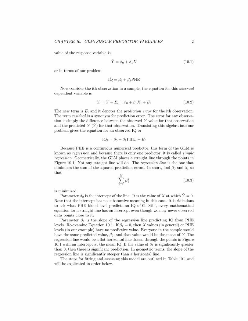
10.1 A single quantitative predictorPhenylketonuria (PKU) is a recessive genetic condition in the DNA blueprintfor the enzyme phenylalanine hydroxylase that converts phenylalanine (PHE)to tyrosine. To prevent the deleterious neurological consequences of the disease,children with PKU have their blood levels of phenylalanine monitored and theirdiet adjusted to avoid high levels of phenylalanine. Many studies have examinedthe relationship between PHE blood levels in childhood and adult scores onintelligence tests ([?]). In this problem, we have a single, numeric predictor(blood PHE) and a single numeric variable to be predicted (IQ).
When there is a single explanatory variable, the equation for the predicted
1
CHAPTER 10. GLM: SINGLE PREDICTOR VARIABLES 2
value of the response variable is
Y = β0 + β1X (10.1)
or in terms of our problem,
ˆIQ = β0 + β1PHE
Now consider the ith observation in a sample, the equation for this observed
dependent variable is
Yi = Y + Ei = β0 + β1Xi + Ei (10.2)
The new term is Ei and it denotes the prediction error for the ith observation.The term residual is a synonym for prediction error. The error for any observa-tion is simply the difference between the observed Y value for that observationand the predicted Y (Y ) for that observation. Translating this algebra into ourproblem gives the equation for an observed IQ or
IQi = β0 + β1PHEi + Ei
Because PHE is a continuous numerical predictor, this form of the GLM isknown as regression and because there is only one predictor, it is called simple
regression. Geometrically, the GLM places a straight line through the points inFigure 10.1. Not any straight line will do. The regression line is the one thatminimizes the sum of the squared prediction errors. In short, find β0 and β1 sothat
N�
i=1
E2i (10.3)
is minimized.Parameter β0 is the intercept of the line. It is the value of X at which Y = 0.
Note that the intercept has no substantive meaning in this case. It is ridiculousto ask what PHE blood level predicts an IQ of 0! Still, every mathematicalequation for a straight line has an intercept even though we may never observeddata points close to it.
Parameter β1 is the slope of the regression line predicting IQ from PHElevels. Re-examine Equation 10.1. If β1 = 0, then X values (in general) or PHElevels (in our example) have no predictive value. Everyone in the sample wouldhave the same predicted value, β0, and that value would be the mean of Y. Theregression line would be a flat horizontal line drawn through the points in Figure10.1 with an intercept at the mean IQ. If the value of β1 is significantly greaterthan 0, then there is significant prediction. In geometric terms, the slope of theregression line is significantly steeper than a horizontal line.
The steps for fitting and assessing this model are outlined in Table 10.1 andwill be explicated in order below.
CHAPTER 10. GLM: SINGLE PREDICTOR VARIABLES 3
Figure 10.1: A scatterplot of blood PHE levels and IQ.
●
●
●
●
●
●
●
●
●
●
●
●
●
●
●
●
●
●
●●
●
●
●
●
●
●
●
●
●
●●
●
●
●●
●
4 6 8 10 12 14
6080
100
120
Blood PHE (100 µmol/l)
IQ
Table 10.1: Fitting and evaluating a GLM with a single quantitative predictor.
1. Inspect the data.
(a) Are there influential data points (outliers)?(b) Do the points suggest linearity?(c) Do the points suggest a mixture of two groups?
2. Fit the model and examine the output.
(a) Does the model ANOVA table indicate significance?(b) What are the parameter estimates?(c) What is the effect size?
3. Check that statistical assumptions are met. Are the errors ...
(a) Normally distributed?(b) Homoscedastic?
CHAPTER 10. GLM: SINGLE PREDICTOR VARIABLES 4
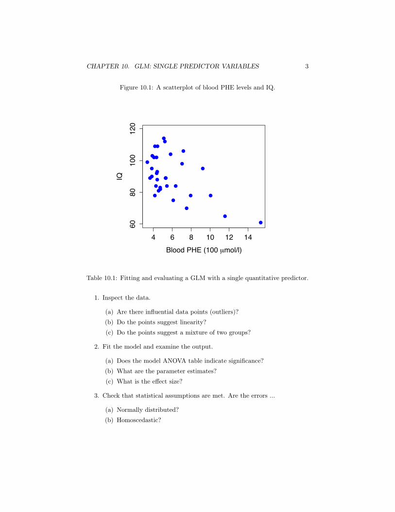
Figure 10.2: Examples of the effects of outliers.
●●
●●
●
●
●●
● ●
●
●●
●
●
R = 0.79 (without)R = −0.071 (with)
● ●
●
●
●
●●
●●
●
●
●
●
●
●
R = −0.082 (without)R = 0.64 (with)
10.1.1 Inspect the dataAs always, the very first task is to inspect the data. The best tool for thisis a scatterplot, a plot of each observation in the sample in two dimensionalspace (see Section X.X). The scatterplot for these data was given in Figure10.1. When the number of observations is large, a scatterplot will resemble anellipse. If the points resemble a circle (a special case of an ellipse), then thereis no relationship between X and Y. As the ellipse becomes more and moreovalish, the relationship increases. Finally, at its limit when the correlation is1.0 or -1.0, ellipse collapses into a straight line.
The three major issue for inspection are: (1) influential data points; (2)nonlinearity; and (3) mixtures of groups.
10.1.1.1 Influential data points (outliers)
The term influential data points refers to observations that have a large effecton the results of a GLM. Advanced GLM diagnostics have been developed toidentify these. In the case of only a single predictor, an influential data pointcan be detected visually in a scatterplot as an outlier.
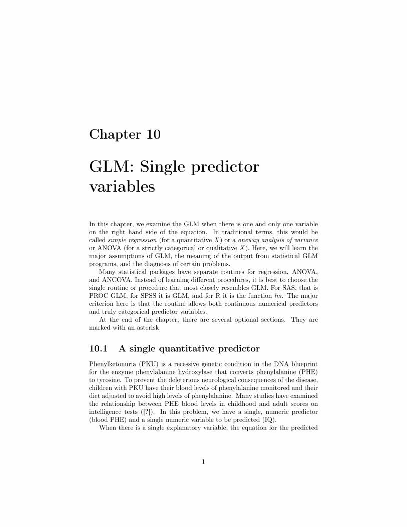
The effect of an outlier is unpredictable. Figure 10.2 demonstrates twopossible effects. Here, the blue circles are the data without the outlier and thered square denotes the outlier. In the left hand panel analysis of all the datapoints gives a correlation close to 0. When the outlier is removed, however, thecorrelation is large and significant. The right panel illustrates just the opposite.The effect of the outlier here is to induce a correlation.
My data have outliers. What should I do? First, refer to section X.X andrecall the difference between a blunder and a rogue. Blunders should definitelybe corrected or, if that is not possible, eliminated. Rouges are a more difficult
CHAPTER 10. GLM: SINGLE PREDICTOR VARIABLES 5
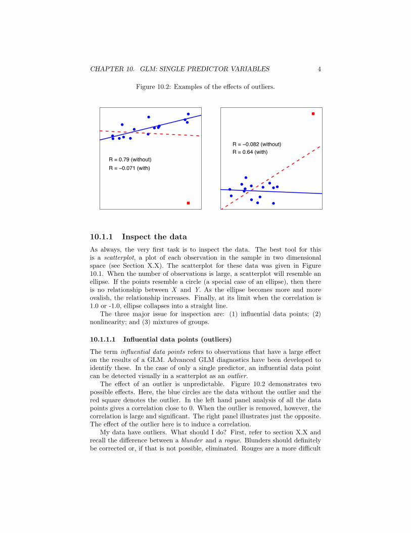
Figure 10.3: Common examples of nonlinear relationships.
●
●●
●
●
●
●●
●
●
●
●
●
●
●
●
●
●
●
●
●
●
●●
●
●
●
●
●
●
●
●
●
●
●
●
●
●
●
●
●
●
●●
●
●
●
●
●
●
issue. The best strategy is to analyze the data with and without the roguevalues and report both results.
10.1.1.2 Nonlinearity
Nonlinearity occurs when the galaxy of points has a regular shape that is notlike an ellipse. The most frequently forms resemble an arc, a U, or an invertedU. Figure 10.3illustrates two types of nonlinear scatterplots.
What is the effect of ignoring a nonlinear relationship and fitting a GLMwith a single predictor? Look at the left panel of Figure 10.3 and mentally drawa straight line that goes through the points. That line would have a strongpositive slope. Hence, the GLM would likely be significant. Here, one wouldcorrectly conclude that X and Y are related, but the form of the relationshipwould be misspecified and the prediction would not be as strong as it could be.
On the other hand, the mental line drawn through the points in the righthand side of the figure would be close to horizontal. The scatterplot shows astrong and regular relationship between the two variables but the GLM wouldfail to detect it.
What to do about nonlinearity? One answer is surprising–use GLM! Theproblem with nonlinearity here is that there is only a single predictor. A tech-nique called polynomial regression adds predictor variables like the square orcube of X to the right hand side of the equation. The plot of Y against X inthis case is a curve instead of a straight line. Section X.X explains this method.
In other cases, transformation(s) of the X and/or Y variables may make therelationship linear. Finally, if there is a strong hypothesis about the mathemat-ical form behind the relationship, one can fit that model to the data. ChapterX.X explains how to do this.
CHAPTER 10. GLM: SINGLE PREDICTOR VARIABLES 6
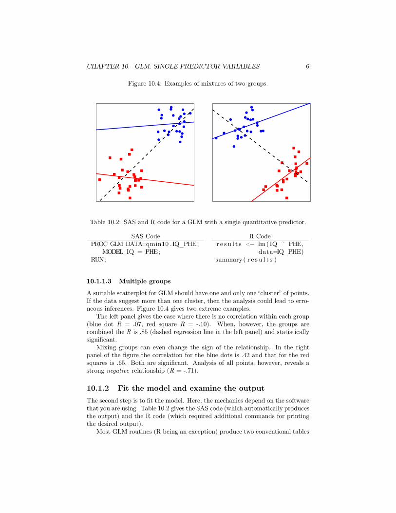
Figure 10.4: Examples of mixtures of two groups.
●
●
●
●
●
●●
●
●
●
●
● ●
●●
●
●●
●
●
●
●●
●
●
●
●●
●
●●●
●●
●
●
●
●
●
●
●
●
●
●
●
●
●●●
●
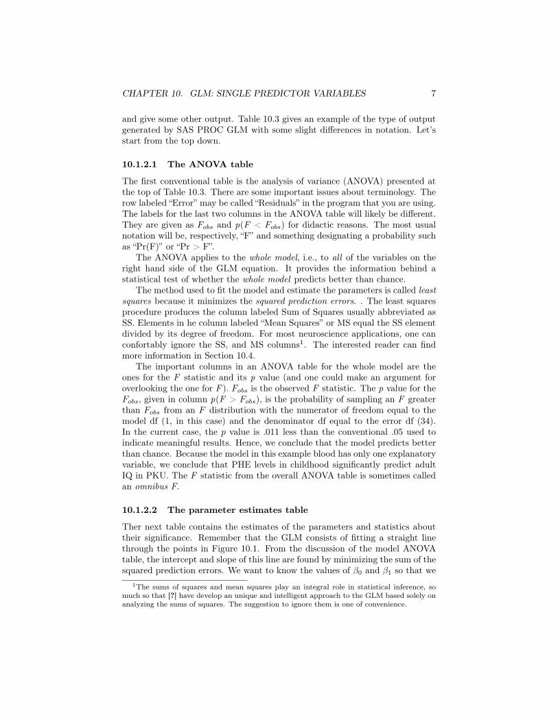
Table 10.2: SAS and R code for a GLM with a single quantitative predictor.
SAS Code R CodePROC GLM DATA=qmin10 .IQ_PHE;
MODEL IQ = PHE;RUN;
r e s u l t s <− lm( IQ ~ PHE,data=IQ_PHE)
summary( r e s u l t s )
10.1.1.3 Multiple groups
A suitable scatterplot for GLM should have one and only one “cluster” of points.If the data suggest more than one cluster, then the analysis could lead to erro-neous inferences. Figure 10.4 gives two extreme examples.
The left panel gives the case where there is no correlation within each group(blue dot R = .07, red square R = -.10). When, however, the groups arecombined the R is .85 (dashed regression line in the left panel) and statisticallysignificant.
Mixing groups can even change the sign of the relationship. In the rightpanel of the figure the correlation for the blue dots is .42 and that for the redsquares is .65. Both are significant. Analysis of all points, however, reveals astrong negative relationship (R = -.71).
10.1.2 Fit the model and examine the outputThe second step is to fit the model. Here, the mechanics depend on the softwarethat you are using. Table 10.2 gives the SAS code (which automatically producesthe output) and the R code (which required additional commands for printingthe desired output).
Most GLM routines (R being an exception) produce two conventional tables
CHAPTER 10. GLM: SINGLE PREDICTOR VARIABLES 7
and give some other output. Table 10.3 gives an example of the type of outputgenerated by SAS PROC GLM with some slight differences in notation. Let’sstart from the top down.
10.1.2.1 The ANOVA table
The first conventional table is the analysis of variance (ANOVA) presented atthe top of Table 10.3. There are some important issues about terminology. Therow labeled “Error” may be called “Residuals” in the program that you are using.The labels for the last two columns in the ANOVA table will likely be different.They are given as Fobs and p(F < Fobs) for didactic reasons. The most usualnotation will be, respectively, “F” and something designating a probability suchas “Pr(F)” or “Pr > F”.
The ANOVA applies to the whole model, i.e., to all of the variables on theright hand side of the GLM equation. It provides the information behind astatistical test of whether the whole model predicts better than chance.
The method used to fit the model and estimate the parameters is called least
squares because it minimizes the squared prediction errors. . The least squaresprocedure produces the column labeled Sum of Squares usually abbreviated asSS. Elements in he column labeled “Mean Squares” or MS equal the SS elementdivided by its degree of freedom. For most neuroscience applications, one canconfortably ignore the SS, and MS columns1. The interested reader can findmore information in Section 10.4.
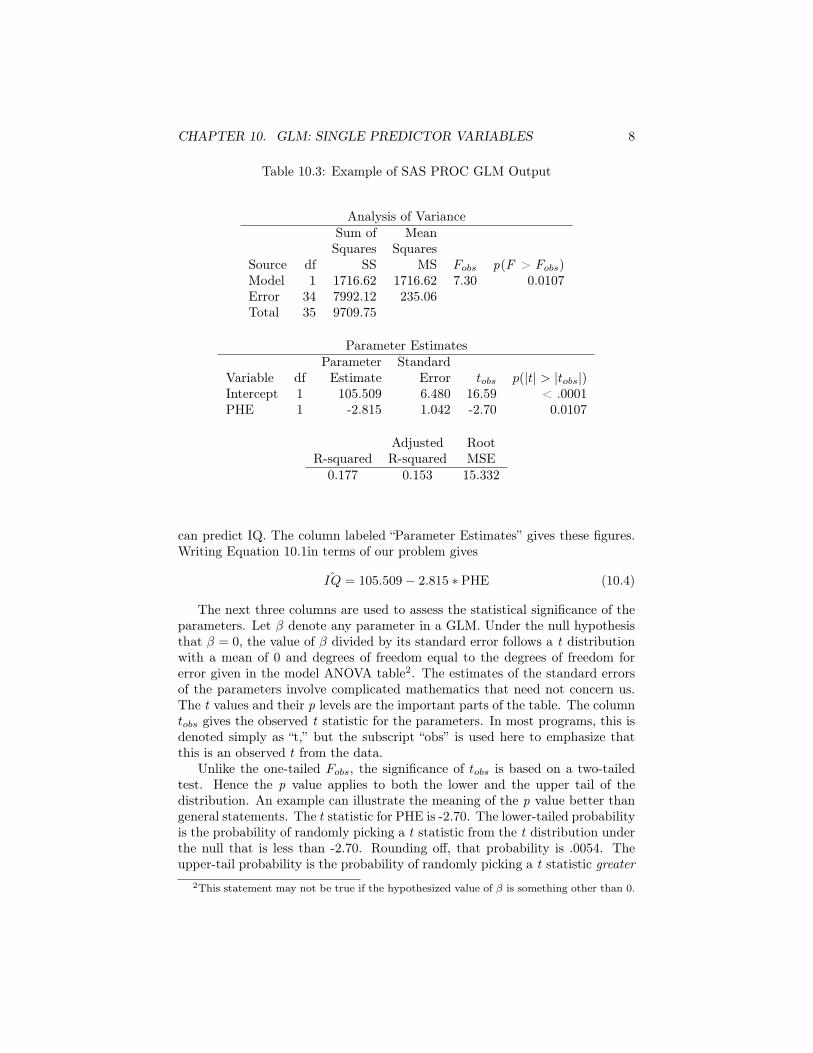
The important columns in an ANOVA table for the whole model are theones for the F statistic and its p value (and one could make an argument foroverlooking the one for F ). Fobs is the observed F statistic. The p value for theFobs, given in column p(F > Fobs), is the probability of sampling an F greaterthan Fobs from an F distribution with the numerator of freedom equal to themodel df (1, in this case) and the denominator df equal to the error df (34).In the current case, the p value is .011 less than the conventional .05 used toindicate meaningful results. Hence, we conclude that the model predicts betterthan chance. Because the model in this example blood has only one explanatoryvariable, we conclude that PHE levels in childhood significantly predict adultIQ in PKU. The F statistic from the overall ANOVA table is sometimes calledan omnibus F.
10.1.2.2 The parameter estimates table
Ther next table contains the estimates of the parameters and statistics abouttheir significance. Remember that the GLM consists of fitting a straight linethrough the points in Figure 10.1. From the discussion of the model ANOVAtable, the intercept and slope of this line are found by minimizing the sum of thesquared prediction errors. We want to know the values of β0 and β1 so that we
1The sums of squares and mean squares play an integral role in statistical inference, somuch so that [?] have develop an unique and intelligent approach to the GLM based solely onanalyzing the sums of squares. The suggestion to ignore them is one of convenience.
CHAPTER 10. GLM: SINGLE PREDICTOR VARIABLES 8
Table 10.3: Example of SAS PROC GLM Output
Analysis of VarianceSum of MeanSquares Squares
Source df SS MS Fobs p(F > Fobs)Model 1 1716.62 1716.62 7.30 0.0107Error 34 7992.12 235.06Total 35 9709.75
Parameter EstimatesParameter Standard
Variable df Estimate Error tobs p(|t| > |tobs|)Intercept 1 105.509 6.480 16.59 < .0001PHE 1 -2.815 1.042 -2.70 0.0107
Adjusted RootR-squared R-squared MSE
0.177 0.153 15.332
can predict IQ. The column labeled “Parameter Estimates” gives these figures.Writing Equation 10.1in terms of our problem gives
ˆIQ = 105.509− 2.815 ∗ PHE (10.4)
The next three columns are used to assess the statistical significance of theparameters. Let β denote any parameter in a GLM. Under the null hypothesisthat β = 0, the value of β divided by its standard error follows a t distributionwith a mean of 0 and degrees of freedom equal to the degrees of freedom forerror given in the model ANOVA table2. The estimates of the standard errorsof the parameters involve complicated mathematics that need not concern us.The t values and their p levels are the important parts of the table. The columntobs gives the observed t statistic for the parameters. In most programs, this isdenoted simply as “t,” but the subscript “obs” is used here to emphasize thatthis is an observed t from the data.
Unlike the one-tailed Fobs, the significance of tobs is based on a two-tailedtest. Hence the p value applies to both the lower and the upper tail of thedistribution. An example can illustrate the meaning of the p value better thangeneral statements. The t statistic for PHE is -2.70. The lower-tailed probabilityis the probability of randomly picking a t statistic from the t distribution underthe null that is less than -2.70. Rounding off, that probability is .0054. Theupper-tail probability is the probability of randomly picking a t statistic greater
2This statement may not be true if the hypothesized value of β is something other than 0.
CHAPTER 10. GLM: SINGLE PREDICTOR VARIABLES 9
than 2.70 from the null t distribution. That probability is also .0054. Hencethe probability of randomly selecting a t more extreme in either direction thanthe one we observed is .0054 + .0054 = .0108 which is within rounding error ofthe value in Table 10.3.
Usually, any statistical inference about β0 being significantly different from0 is uninteresting. One can artificially manipulate the significance of β0 bychanging the scales of measurement for the X and Y variables. One wouldalways get the same predicted values relative to the scale changes; only thesignificance could change.
The t statistic for the predictability of PHE levels is -2.70 and its p value is.01. Hence, we conclude that blood PHE values significantly predict IQ. Beforeleaving this table, compare the p value from the F statistic in the model ANOVAtable to the p for the t statistic in the Parameter Estimates table. They areidentical! This is not an aberration. It will always happen when there is onlyone predictor. Can you deduce why?3
A little algebra can help us to understand the substantive meaning of a GLMcoefficient for a variable. Let’s fix the value of X to a specific number, say, X∗.Then the predicted value for Y at this value is
YX∗ = β0 + β1X∗ (10.5)
Change the value of X∗ by adding exactly 1 to it. The predicted value underthis case is
YX∗+1 = β0 + β1 (X∗+ 1) (10.6)
Finally, subtract the previous equation from this one
YX∗+1 − YX∗ = β0 + β1X∗+ β1 − β0 − β1X
∗
soβ1 = YX∗+1 − YX∗ (10.7)
In words, the right side of Equation 10.7 is the change in the predicted valueof Y when X is increased by one unit. In other terms, the β for a variable givesthe predicted change in Y for a one unit increase in X. This is a very importantdefinition. It must be committed to memory.
In terms of the example, the β for PHE is -2.815. Hence, a one unit increasein blood PHE predicts a decrease in IQ of -2.815. Given that the measurementof blood PHE is in terms of 100 µl/l (see the horizontal axis in Figure 10.1), weconclude at change blood PHE from 300 to 400 µl/l predicts a decrease in IQof 2.8 points.
3Recall that the model ANOVA table gives the results of predictability for the whole model.It just so happens that the “whole model” in this case has only one predictor variable, PHE.Hence the significance level for the whole model is the same as that for the coefficient forPHE.
CHAPTER 10. GLM: SINGLE PREDICTOR VARIABLES 10
10.1.2.3 Other Output
Usually, output from GLM contains other statistics. One very important statis-tic is the squared multiple correlation or R2. This is the square of the correlationbetween observed values of the dependent variable (Y ) and their predicted val-ues (Y ). Recall the meaning of a squared correlation. It is a quantitativeestimate of the proportion of variance in one variable predicted by or attributedto the other variable. Hence, R2 gives the proportion of variance in the depen-dent variable attributed to its predicted values. Given that the predicted valuescome from the model, the best definition is: R
2 equals the proportion of vari-
ance in the dependent variable predicted by to the model. You should memorizethis definition. Understanding R
2 is crucial to understanding GLM. Indeed,comparison of different linear models predicting the same dependent variable isbest done using R
2. Also, R2 is the standard measure of effect size in a GLM.There are several ways to give equations for R
2. Here are some of them
R2= corr
�Y, Y
�2=
σ2Y
σ2Y
= 1− σ2E
σ2Y
=SSTotal − SSError
SSTotal(10.8)
You should memorize the first three terms on the right hand side of this equation.The third term allows you to calculated R
2 from an ANOVA table. In the dataat hand, R
2 = .177. Hence, blood phenylalanine levels predict 18% of thevariance in adult IQ in this sample of phenylketonurics.
Although R2 is the summary statistic most often cited for the explanatory
power of a model, is it a biased statistic. The amount of bias, however, is acomplicated function of sample size and the number of predictors. In manycases, the bias is not entirely known. A statistic that attempts to account forthis bias is the adjusted R
2. When sample size is large there is little differencebetween R
2 and adjusted R2. For these data, adjusted R
2 = .153.A cautionary note about R2: these statistics can differ greatly in laboratory
experimental designs from real world, observational, designs on humans. In allbut rare cases, the causes of human behavior are highly multifactorial. Hence,the study of only a few hypothesized etiological variables will not predict a greatamount of the variance in behavior. R
2 is usually small here. Within the lab,however, many experimental designs allow very large manipulations. These cangenerate much larger R
2s.The final statistic in Table 10.3 is called “Root MSE” which is the square
root of the mean squares for error. Sometimes this is “aconymized” as RMSE.In a GLM, the “mean squares for error” is synonymous with the estimation ofthe variance of the prediction errors aka residuals. The square root of a varianceis, of course, the standard deviation, so RMSE is an estimate of the standarddeviation of prediction errors. The number, 15.3 in this case, has little meaningin itself. Instead, it is used to compare one GLM to another for the same Y.When the differences in R
2 and in RSME are relatively large, then the modelwith the higher R
2, or in different terms, lower RMSE, is to be preferred.
CHAPTER 10. GLM: SINGLE PREDICTOR VARIABLES 11
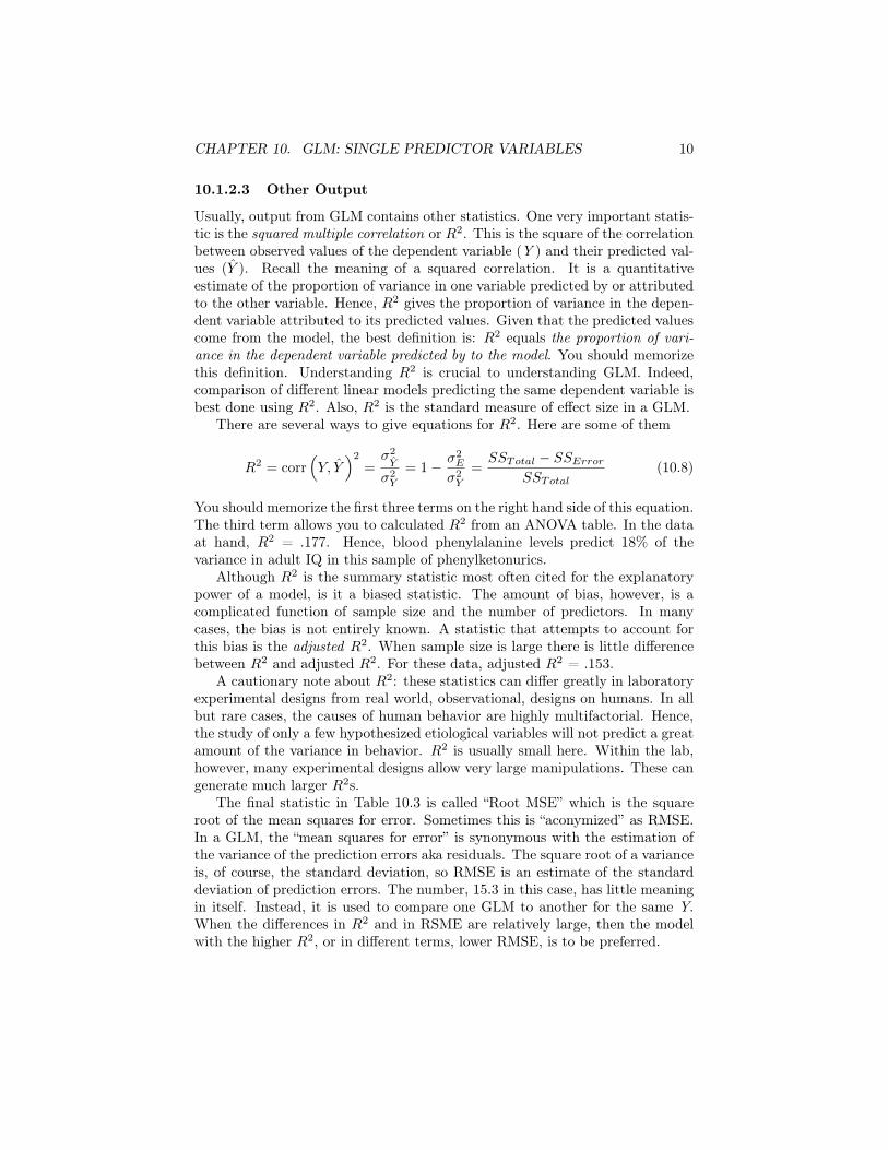
Figure 10.5: QQ plot for IQ residuals.
●●
●
●●
●
●
●
●
●
●
●
●
●
●
●●
●●
●
●
●
●
●
●
●
●
●●
●
●
●
●
●●●
−2 −1 0 1 2
−40
−20
020
Theoretical Quantiles
IQ R
esid
ual
10.1.3 Diagnose the resultsIn step 3, we assess the results to see how well they meet the assumptions ofthe GLM. Whole books have been written about GLM diagnostics ([?, ?]), sothe treatment here is limited to those situations most frequently encountered inneuroscience.
A valid F statistic has two major assumptions involving the prediction errorsor residuals: (1) they are normally distributed; and (2) they have the samevariance across all values of the predictor variables. The normality assumptionis usually assessed via a QQ plot (see Section X.X) of the residuals, given inFigure 10.5 for the PKU data. Because the actual residuals are close to thestraight line (which, recall, is their predicted distribution if they were exactlynormal), the assumption of normality is robust.
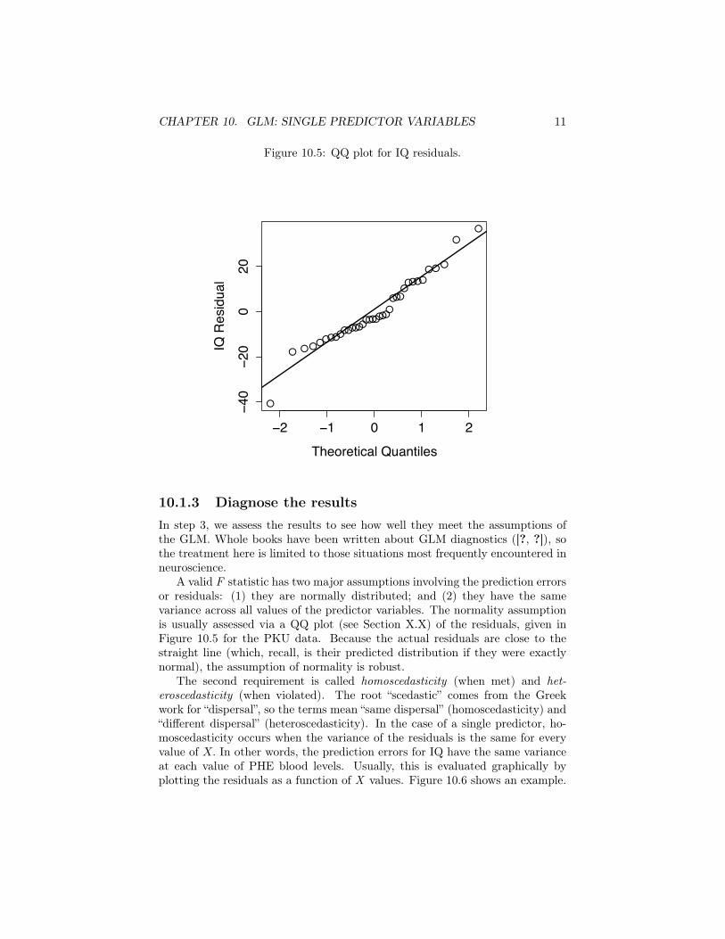
The second requirement is called homoscedasticity (when met) and het-
eroscedasticity (when violated). The root “scedastic” comes from the Greekwork for “dispersal”, so the terms mean “same dispersal” (homoscedasticity) and“different dispersal” (heteroscedasticity). In the case of a single predictor, ho-moscedasticity occurs when the variance of the residuals is the same for everyvalue of X. In other words, the prediction errors for IQ have the same varianceat each value of PHE blood levels. Usually, this is evaluated graphically byplotting the residuals as a function of X values. Figure 10.6 shows an example.
CHAPTER 10. GLM: SINGLE PREDICTOR VARIABLES 12
Figure 10.6: Examination of homoscedasticity for the residuals for IQ.
●●
●
●●
●
●
●
●
●
●
●
●
●
●
●●
● ●
●
●
●
●
●
●
●
●
●●
●
●
●
●
●●●
4 6 8 10 12 14
−40
−20
020
Blood PHE (100 µmol/l)
Res
idua
l
Normally, detection of heteroscedasticity requires very large sample sizes–say, a 10 fold increase over the present one. In Figure 10.6 there is widerdispersion at lower blood levels than higher ones, but this could have easilyhappen by chance. There are two few observations sampled at higher levels tomake any strong conclusion.
This situation is not unique and will likely be the case for laboratory-basedstudies. A good case could be made to ignore heteroscedasticity altogether insuch research. In epidemiological neuroscience, however, where sample sizes canbe in the tens of thousands, one should always mindful of the problem.
10.1.4 Report the ResultsAs always, the detail of any GLM report depends on how integral the analysisis to the overall mission of the publication. Suppose the analysis is importantonly in the minor sense that it demonstrates that your data agree with previouspublications. Here a mention of either the correlation coefficient or the slopeof the regression line would be sufficient along with information on significance.An example would be: “Consistent with other studies we round a significant,negative relationship between childhood PHE levels in blood and adult IQ (R =
−.42, N = 36, p = .01)”. This reports the correlation coefficient. You could
CHAPTER 10. GLM: SINGLE PREDICTOR VARIABLES 13
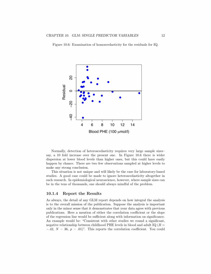
Figure 10.7: Example of a plot for publication.
●
●
●
●
●
●
●
●
●
●
●
●
●
●
●
●
●
●
●●
●
●
●
●
●
●
●
●
●
●●
●
●
●●
●
4 6 8 10 12 14
6080
100
120
Blood PHE (100 µmol/l)
IQIQ = 107.51 − 2.815*PHE
also report the GLM coefficient, but here it is customary to give the degrees offreedom rather than sample size. Some journals require that you report the teststatistic, the t statistic in this case. In this case, using t34 or t(34) may suffice.Naturally, you should always express the results in the preferred format of thepublication. If you do report the GLM coefficient, consider also reporting R
2
to inform the reader of effect size.When the GLM is an integral part of the report, consider a figure such as
the one in Figure 10.1 that has the regression line and the regression equation.In the text, give R
2, the test statistic for the model (either the F or the t willdo), and the p value.
10.2 A single qualitative predictorIt has been widely known that the genetic background of animals can influenceresults in neuroscience. As part of a larger project examining differences ininbred strains of mice and laboratory effects, [?] tested eight different strainson their activity in an open field before and after the administration of cocaine.Here, we consider a simulated data set based on the above study where thedependent variable is the difference score in activity before and after the drug.
In this case the dependent variable is Activity and the independent or pre-
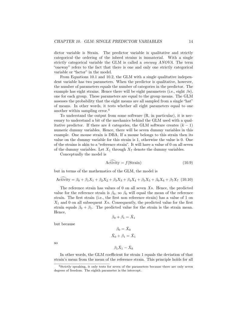
CHAPTER 10. GLM: SINGLE PREDICTOR VARIABLES 14
dictor variable is Strain. The predictor variable is qualitative and strictlycategorical–the ordering of the inbred strains is immaterial. With a singlestrictly categorical variable the GLM is called a oneway ANOVA. The term“oneway” refers to the fact that there is one and only one strictly categoricalvariable or “factor” in the model.
From Equations 10.1 and 10.2, the GLM with a single qualitative indepen-dent variable has two parameters. When the predictor is qualitative, however,the number of parameters equals the number of categories in the predictor. Theexample has eight strains. Hence there will be eight parameters (i.e., eight βs),one for each group. These parameters are equal to the group means. The GLMassesses the probability that the eight means are all sampled from a single “hat”of means. In other words, it tests whether all eight parameters equal to oneanother within sampling error.4
To understand the output from some software (R, in particular), it is nec-essary to understand a bit of the mechanics behind the GLM used with a qual-itative predictor. If there are k categories, the GLM software creates (k − 1)
numeric dummy variables. Hence, there will be seven dummy variables in thisexample. One mouse strain is DBA. If a mouse belongs to this strain then itsvalue on the dummy variable for this strain is 1, otherwise the value is 0. Oneof the strains is akin to a “reference strain”. It will have a value of 0 on all sevenof the dummy variables. Let X1 through X7 denote the dummy variables.
Conceptually the model is
�Activity = f(Strain) (10.9)
but in terms of the mathematics of the GLM, the model is
�Activity = β0 + β1X1 + β2X2 + β3X3 + β4X4 + β5X5 + β6X6 + β7X7 (10.10)
The reference strain has values of 0 on all seven X s. Hence, the predictedvalue for the reference strain is β0, so β0 will equal the mean of the referencestrain. The first strain (i.e., the first non reference strain) has a value of 1 onX1 and 0 on all subsequent X s. Consequently, the predicted value for the firststrain equals β0 + β1. The predicted value for the strain is the strain mean.Hence,
β0 + β1 = X1
but becauseβ0 = X0
X0 + β1 = X1
soβ1X1 − X0
In other words, the GLM coefficient for strain 1 equals the deviation of thatstrain’s mean from the mean of the reference strain. This principle holds for all
4Strictly speaking, it only tests for seven of the parameters because there are only sevendegrees of freedom. The eighth parameter is the intercept.
CHAPTER 10. GLM: SINGLE PREDICTOR VARIABLES 15
Table 10.4: Fitting and evaluating a GLM with a single qualitative predictor.
1. Do you really want to use a qualitative predictor?
2. Inspect the data
(a) Are there influential data points (outliers)?(b) Are there normal distributions within groups?(c) Are the variances homogeneous?
3. Fit the model and examine the output.
(a) Does the model ANOVA table indicate significance?(b) Do tests indicate homogeneity of variance?(c) [Optional] What do the parameter estimates suggest?(d) [Optional] What do multiple group comparisons indicate about the
group means?(e) What is the effect size?
of the other non reference strains. For example β5 is the the difference betweenstrain five’s mean and the mean of the reference strain. Hence, the statisticaltests for β1 through β7 measure whether a strain’s mean is significantly differentfrom the reference strain. Good GLM procedures allow you to specify whichcategory will be the reference category. It is useful to make this the controlgroup so that you can test those groups that are significantly different from thecontrols.
The null hypothesis for the GLM in a oneway ANOVA is that β1 through βk
are all within sampling error of 0. In words, the null hypothesis states for theinbred strain example maintains that all eight strain means are sampled froma “hat” of means with an overall mean of µ and a standard deviation that isestimated by the standard deviations of the groups. The alternative hypothesisis that at least one mean is sampled from a different “hat”.
The procedures for performing, interpreting, and assessing a oneway ANOVAare surprisingly similar to a simple regression. The biggest differences are inpreliminary data screening and informing the GLM that the X variable is qual-itative. They are given in Table 10.4 and explicated below.
10.2.1 Do you really want to use a qualitative predictor?This is the most important question. Do you really want to use a onewayANOVA? Recall the distinction between strictly categorical variables and or-
dered groups. If there is an underlying metric behind the variable, then do not
use a oneway ANOVA, or any other ANOVA for that matter. Ask yourself the
CHAPTER 10. GLM: SINGLE PREDICTOR VARIABLES 16
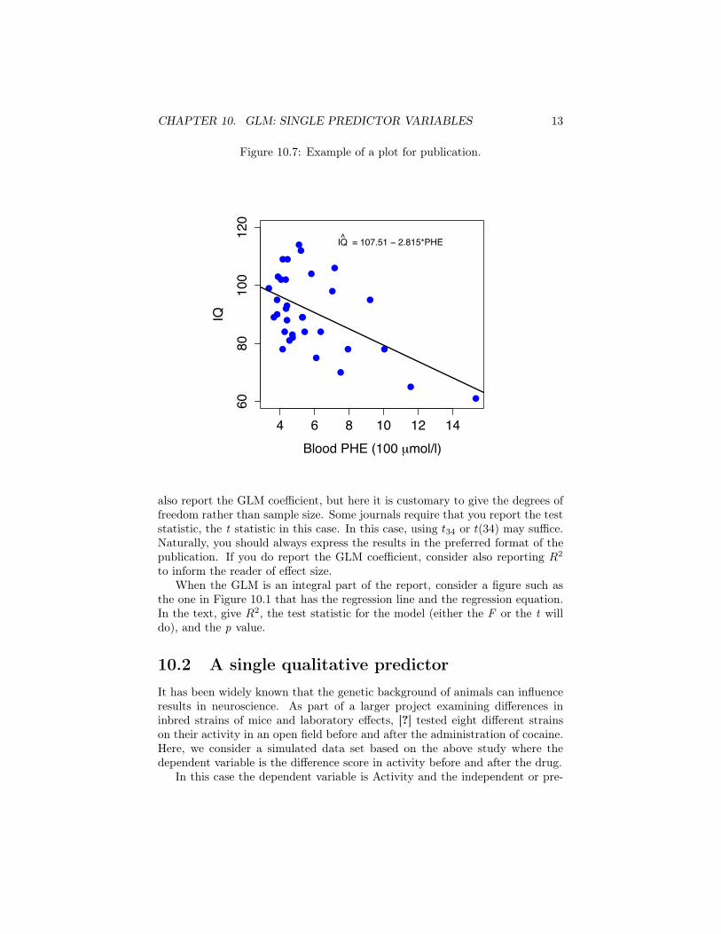
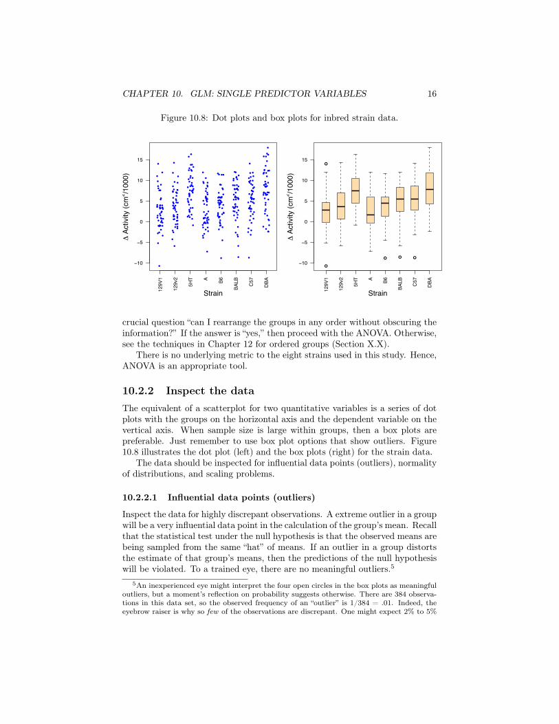
Figure 10.8: Dot plots and box plots for inbred strain data.
129V
1
129v
2
5HT A B6
BALB C57
DBA
−10
−5
0
5
10
15
Strain
Δ A
ctiv
ity (c
m2 /1
000)
●
●
●
●
●
●
●
●
●
●
●
●
●
●
●
●●
●
●
●
●
●
●
●
●●
●
●
●
●●
●
●
●
●●
●
●
●
●
●
●
●
●
●
●
●
●
●●
●
●
●
●
●
●
●
●
●
●
● ●
●
●
●
●
●
●
●
●
●
●
●
●
●
●
●
●
●
●
●
●
●
●●
●
●
●
●
●
●
●
●
●
●
●
●
●
●
●
●
●
●
●
●
●
●
●
●
●
●
●
●
●
●
●
●
●
●
●
●
●
●
●●
●
●
●
●
●
●
●
●
●
●
●
●
●
●
●
●
●●
●
●
●
●
●
●
●
●
●
●
●
●
●
●
●
●
●
●
●
●
●
●
●
●
●●
●
●
●
●
●
●●
●
●
●
●
●
●●
●
●
●
●
●
●
●
●
●
●
●
●
●
●
●
●●
●
●
●
●
●
●
●
●
●
●
●
●
●
●
●
●
●
●
●
●
●
●
●
●
●
●●
●
●
●
●
●
●
●
●
●
●
●
●
●
●
●
●
●
●
●
●
●
●
●●
●
●
●
●
●
●●
●
●
●
●
●
●
●
●
●
●
●
●
●●
●
●●
●
●
●
●
●
●
●
●
●
●
●
●
●
●
●
●
●
●
●
●
●
●
●
●
●
●●
●
●
●●
●
●
●
●
●
●
●
●
●
●
●
●
●
●
●
●
●
●
●
●●
●
●
●
●
●
●
●
●
●
●
●
●
●
●
●
●
●
●
●
●
● ●
●
●●
●
●●
●
●
●
●
●
●
●
●
●
●
●
●
●●
●
●
●
●
●
●●
●
●
●
●
●
●
●
●
●
●
● ● ●
129V
1
129v
2
5HT A B6
BALB C57
DBA
−10
−5
0
5
10
15
StrainΔ
Act
ivity
(cm
2 /100
0)
crucial question “can I rearrange the groups in any order without obscuring theinformation?” If the answer is “yes,” then proceed with the ANOVA. Otherwise,see the techniques in Chapter 12 for ordered groups (Section X.X).
There is no underlying metric to the eight strains used in this study. Hence,ANOVA is an appropriate tool.
10.2.2 Inspect the dataThe equivalent of a scatterplot for two quantitative variables is a series of dotplots with the groups on the horizontal axis and the dependent variable on thevertical axis. When sample size is large within groups, then a box plots arepreferable. Just remember to use box plot options that show outliers. Figure10.8 illustrates the dot plot (left) and the box plots (right) for the strain data.
The data should be inspected for influential data points (outliers), normalityof distributions, and scaling problems.
10.2.2.1 Influential data points (outliers)
Inspect the data for highly discrepant observations. A extreme outlier in a groupwill be a very influential data point in the calculation of the group’s mean. Recallthat the statistical test under the null hypothesis is that the observed means arebeing sampled from the same “hat” of means. If an outlier in a group distortsthe estimate of that group’s means, then the predictions of the null hypothesiswill be violated. To a trained eye, there are no meaningful outliers.5
5An inexperienced eye might interpret the four open circles in the box plots as meaningfuloutliers, but a moment’s reflection on probability suggests otherwise. There are 384 observa-tions in this data set, so the observed frequency of an “outlier” is 1/384 = .01. Indeed, theeyebrow raiser is why so few of the observations are discrepant. One might expect 2% to 5%
CHAPTER 10. GLM: SINGLE PREDICTOR VARIABLES 17
Note that when the number of observations is small within groups, thenboth dot plots and box plots can give results for a group or two that appearaberrant to the eye but are satisfactory for analysis. The GLM is sturdy againstmoderate violations for its assumptions, so do not be too obsessional aboutdetecting outliers. As always, if you do detect an extreme data point, determinewhether it is a rogue or a blunder. If possible, correct blunders. Substantiveconsiderations should be used to deal with rogues.
10.2.2.2 Normal distributions within groups
With a quantitative predictor, an assumption for the test of significance is thatthe residuals are normally distributed. The analogous assumption with a quali-tative predictor is that the residuals are normally distributed within each group.Because the predicted value of the dependent variable for a group is the groupmean, the assumption implies that the distribution of scores within each groupis normal.
One could examine QQ plots for normality within each group, but that usu-ally unnecessary. A large body of research had shown that the GLM for asingle qualitative predictor is robust to moderate violations of the normalityassumption. Hence, visual inspection of the points should be directed to assess-ing different clusters of points within a group and cases of extreme skewnesswhere most values for a group are clustered at one end. If you see problems, tryrescaling the data. If that does not produce satisfactory distributions then youshould use a non parametric test such as the Mann Whitney U test.
10.2.2.3 Homogeneity of variance and scaling problems
The assumption of homogeneity of variance is actually the assumption of ho-moscedasticity applied to groups. Recall that homoscedasticity is defined as theproperty that the variance of the residuals (aka prediction errors) is the same atevery point on the regression line. With a categorical predictor with k groups,the predicted values are the group means and the residuals are the deviationsof the raw scores from their respective group mean. Hence, the assumption isthat the variance within each group is the same (aka homogeneous).
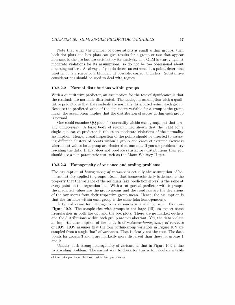
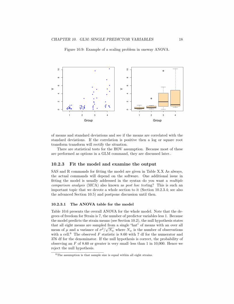
A typical cause for heterogeneous variances is a scaling issue. ExamineFigure 10.9. The sample size with groups is not large (15), so expect someirregularities in both the dot and the box plots. There are no marked outliersand the distributions within each group are not aberrant. Yet, the data violatean important assumption of the analysis of variance–homogeneity of variance
or HOV. HOV assumes that the four within-group variances in Figure 10.9 aresampled from a single “hat” of variances. That is clearly not the case. The datapoints for groups 3 and 4 are markedly more dispersed than those for groups 1and 2.
Usually, such strong heterogeneity of variance as that in Figure 10.9 is dueto a scaling problem. The easiest way to check for this is to calculate a table
of the data points in the box plot to be open circles.
CHAPTER 10. GLM: SINGLE PREDICTOR VARIABLES 18
Figure 10.9: Example of a scaling problem in oneway ANOVA.
1 2 3 4
02
46
810
Group
Y
●●●
●
●●● ●●
●●
●●
●●
●
●
●
●●
●
●
●
●
●
●
●●
●●
●
●
●
●
●
●
●
●
●
●
●
●
●
●
●
●
●
●
●●
●
●
●
●
●
●●
●
●
●
●
●
1 2 3 4
02
46
810
GroupY
of means and standard deviations and see if the means are correlated with thestandard deviations. If the correlation is positive then a log or square roottransform transform will rectify the situation.
There are statistical tests for the HOV assumption. Because most of theseare performed as options in a GLM command, they are discussed later..
10.2.3 Fit the model and examine the outputSAS and R commands for fitting the model are given in Table X.X As always,the actual commands will depend on the software. One additional issue infitting the model is usually addressed in the syntax–do you want a multiple
comparison analysis (MCA) also known as post hoc test ing? This is such animportant topic that we devote a whole section to it (Section 10.2.3.4; see alsothe advanced Section 10.5) and postpone discussion until then.
10.2.3.1 The ANOVA table for the model
Table 10.6 presents the overall ANOVA for the whole model. Note that the de-grees of freedom for Strain is 7, the number of predictor variables less 1. Becausethe model predicts the strain means (see Section 10.2), the null hypothesis statesthat all eight means are sampled from a single “hat” of means with an over allmean of µ and a variance of σ2
/√Nw where Nw is the number of observations
with a cell.6 The observed F statistic is 8.60 with 7 df for the numerator and376 df for the denominator. If the null hypothesis is correct, the probability ofobserving an F of 8.60 or greater is very small–less than 1 in 10,000. Hence wereject the null hypothesis.
6The assumption is that sample size is equal within all eight strains.

CHAPTER 10. GLM: SINGLE PREDICTOR VARIABLES 19
Table 10.5: SAS and R code for a GLM with a single qualitative predictor.
SAS CodePROC GLM DATA=qmin10 . crabbe ;
CLASS St ra in ;MODEL Act iv i ty = St ra in ;MEANS Stra in / HOVTEST=Levene ;
RUN;
R Coder e s u l t s <− lm( Act i v i t y ~ Stra in , data=crabbe )summary( r e s u l t s )# the car package conta in s the Levene HOV t e s tl i b r a r y ( car )l eveneTest ( r e s u l t s , c en t e r=mean)
Table 10.6: Model overall ANOVA table for strain differences.
Overall ANOVAdf SS MS Fobs p(F > Fobs)
Strain 7 1239.03 177.00 8.60 < 0.0001Residuals 376 7740.18 20.59
Total 383 8979.21
CHAPTER 10. GLM: SINGLE PREDICTOR VARIABLES 20
The alternative hypothesis for a oneway ANOVA states that “at least onemean, but possibly more, is sampled from a different hat than the others.” Theresults give strong support for the alternative hypothesis so somewhere thereare mean differences among the strains. But where? Perhaps the parameterestimates will give us a clue.
10.2.3.2 Homogeneity of variance
Most tests for HOV are called as options to a GLM statement. There are severaldifferent HOV tests, but Levene’s (1960) test is widely acknowledged as one ofthe better ones. That is the good news. The bad news is that there are threedifferent varieties of Levene’s test: (1) Levene’s testing using the absolute valueof the difference from the mean; (2) Levene’s test using squared differences fromthe mean; and (3) Levene’s test using the absolute value of the difference fromthe median. You may see the last of these refered to as the Brown-Forsythe test([?]). Most of the time, these tests will lead to the same conclusion.
On these data, Levene’s test gives the following statistics: F (7, 376) = 0.69,p = .68. There is no evidence for different within-group variances.
10.2.3.3 The parameter estimates
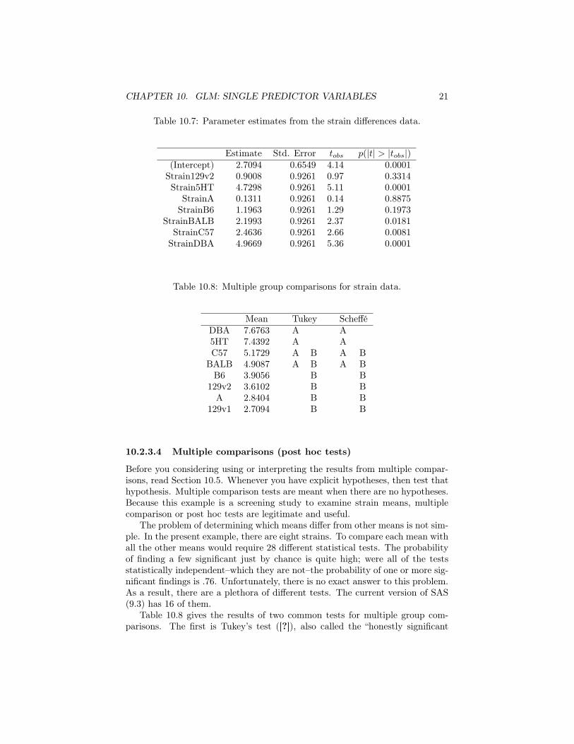
Table 10.7 gives the parameter estimates from the model in Equation 10.10.Recall that the model has an intercept that equals the strain mean for thereference strain. The strains are ordered alphabetically and the software thatperformed the analysis (R) uses the very first level of a factor as the referencegroup. Hence, the value of the intercept (2.71) equals the mean for the very firststrain, 129v1. β1 is the coefficient for dummy code for the next strain, 129v2.Hence the mean of this strain is
X129v2 = β0 + β1 = 2.71 + .90 = 3.61
The lack of significance for coefficient β1 (tobs = .97, p = .33) tells us that themean for strain 129v2 is not different from the mean of strain 129v1.
The next coefficient, β2, if for the dummy variable for strain 5HT. The meanfor this strain is
X5HT = β0 + β1 = 2.71 + 4.73 = 7.44
and the coefficient is significant (tobs = 5.11, p < .0001). Thus, the mean forstrain 5HT is significantly different than the mean for strain 129v1.
If we continue with this, we find that the significance of all the βs, save β0,tests whether the strain mean differs significantly from the 129v1 mean. Thatis somewhat interesting but it leaves unanswered many other questions. Is themean for strain 5HT significantly different from the mean for BALBs? Theregular GLM will not answer that.
CHAPTER 10. GLM: SINGLE PREDICTOR VARIABLES 21
Table 10.7: Parameter estimates from the strain differences data.
Estimate Std. Error tobs p(|t| > |tobs|)(Intercept) 2.7094 0.6549 4.14 0.0001
Strain129v2 0.9008 0.9261 0.97 0.3314Strain5HT 4.7298 0.9261 5.11 0.0001
StrainA 0.1311 0.9261 0.14 0.8875StrainB6 1.1963 0.9261 1.29 0.1973
StrainBALB 2.1993 0.9261 2.37 0.0181StrainC57 2.4636 0.9261 2.66 0.0081
StrainDBA 4.9669 0.9261 5.36 0.0001
Table 10.8: Multiple group comparisons for strain data.
Mean Tukey SchefféDBA 7.6763 A A5HT 7.4392 A AC57 5.1729 A B A B
BALB 4.9087 A B A BB6 3.9056 B B
129v2 3.6102 B BA 2.8404 B B
129v1 2.7094 B B
10.2.3.4 Multiple comparisons (post hoc tests)
Before you considering using or interpreting the results from multiple compar-isons, read Section 10.5. Whenever you have explicit hypotheses, then test thathypothesis. Multiple comparison tests are meant when there are no hypotheses.Because this example is a screening study to examine strain means, multiplecomparison or post hoc tests are legitimate and useful.
The problem of determining which means differ from other means is not sim-ple. In the present example, there are eight strains. To compare each mean withall the other means would require 28 different statistical tests. The probabilityof finding a few significant just by chance is quite high; were all of the testsstatistically independent–which they are not–the probability of one or more sig-nificant findings is .76. Unfortunately, there is no exact answer to this problem.As a result, there are a plethora of different tests. The current version of SAS(9.3) has 16 of them.
Table 10.8 gives the results of two common tests for multiple group com-parisons. The first is Tukey’s test ([?]), also called the “honestly significant
CHAPTER 10. GLM: SINGLE PREDICTOR VARIABLES 22
difference (HSD)” test. The second is Scheffé’s test ([?]). Tukey’s is a well es-tablished and widely used test. Scheffé’s is a conservative test. That is, when itdoes detect differences, there is a very high probability that they are real, butthe false negative rate (not detecting differences that are there) is higher thannormal. In this case, both tests gave identical results.
The results are presented so that all groups with the same letter have nomean differences, That is, there is no significant differences for the means groupA (DBA, 5HT, C57, BALB). Likewise, there are no significant differences amongstrain means within group B (C57, BALB, B6, 129v2, A, and 129v1). Notethat C57s and BALBs belong to both groups. This is not unusual in groupcomparisons. The substantive conclusion is that DBAs and 5HTs have highmeans that are significantly different than the low-mean groups of B6, 129v2,A, and 129v1. C57s and BALBs are intermediate.
10.2.3.5 Examine the effect size.
The R2 for this problem is .12. This indicated that 12% of the variance in
cocaine-induced activity is explained by mean strain differences.
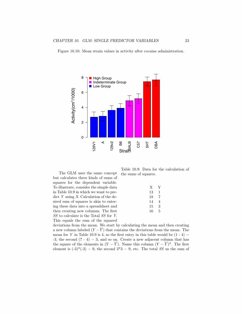
10.2.4 Reporting the ResultsBecause the GLM for a single qualitative variable deals with the group means,most results are reported by a plot of means. Figure 10.10 illustrates a bar chartfor the strain data. To aid visual inspection, the strains are ordered from lowestto highest mean value, and the bars are color coded to denote the groupings fromthe post hoc analysis. In the text, give the overall F, the degrees of freedom,and p value–e.g., F (3, 376) = 8.60, p < .0001. The text should also mentionthat both the Tukey and Scheffé multiple comparisons analyses gave the sameresults–the high group was significantly different from the low group, but theintermediate group did not differ from either the high or the low groups.
10.3 Least squares criterion and sums of squares*The standard way for finding the parameters, i.e.βs, in the GLM is to use theleast squares criterion. This turns out to be a max-min problem in calculus. Wedeal with that later. Now let’s gently introduce the topic through the conceptof the sum of squares. If we have a scores of numbers, say A, the sum of squaresis found by squaring each individual number and then taking its sum,
SSA =
N�
i=1
A2i (10.11)
We have already seen this concept in the calculation of a variance.
CHAPTER 10. GLM: SINGLE PREDICTOR VARIABLES 23
Figure 10.10: Mean strain values in activity after cocaine administration.
129V
1 A
129v
2 B6
BALB C57
5HT
DBA
Strain
Activ
ity(c
m2 /1
000)
0
2
4
6
8 High GroupIndeterminate GroupLow Group
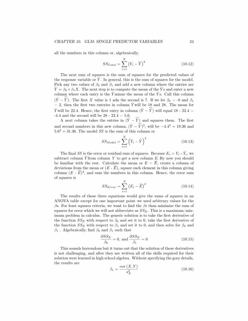
Table 10.9: Data for the calculation ofthe sums of squares.
X Y13 118 714 415 316 5
The GLM uses the same conceptbut calculates three kinds of sums ofsquares for the dependent variable.To illustrate, consider the simple datain Table 10.9 in which we want to pre-dict Y using X. Calculation of the de-sired sum of squares is akin to enter-ing these data into a spreadsheet andthen creating new columns. The firstSS to calculate is the Total SS for Y.This equals the sum of the squareddeviations from the mean. We start by calculating the mean and then creatinga new column labeled (Y −Y ) that contains the deviations from the mean. Themean for Y in Table 10.9 is 4, so the first entry in this table would be (1 - 4) =-3, the second (7 - 4) = 3, and so on. Create a new adjacent column that hasthe square of the elements in (Y − Y ). Name this column (Y − Y )
2. The firstelement is (-3)*(-3) = 9, the second 3*3 = 9, etc. The total SS us the sum of
CHAPTER 10. GLM: SINGLE PREDICTOR VARIABLES 24
all the numbers in this column or, algebraically,
SSTotal =
N�
i=1
�Yi − Y
�2 (10.12)
The next sum of squares is the sum of squares for the predicted values ofthe response variable or Y . In general, this is the sum of squares for the model.Pick any two values of β0 and β1 and add a new column where the entries areY = β0+β1X. The next step is to compute the mean of the Y s and enter a newcolumn where each entry is the Y minus the mean of the Y s. Call this column(Y − Y ). The first X value is 1 adn the second is 7. If we let β0 = -8 and β1
= 2, then the first two enteries in column Y will be 18 and 28. The mean forY will be 22.4. Hence, the first entry in column (Y − Y ) will equal 18 - 22.4 =-4.4 and the second will be 28 - 22.4 = 5.6.
A next column takes the entries in (Y − Y ) and squares them. The firstand second numbers in this new column, (Y − Y )
2, will be −4.42= 19.36 and
5.62= 31.36. The model SS is the sum of this column or
SSModel =
N�
i=1
�Yi − ¯
Y
�2(10.13)
The final SS is the error or residual sum of squares. Because Ei = Yi−Yi, wesubtract column Y from column Y to get a new column E. By now you shouldbe familiar with the rest. Calculate the mean or E = E, create a column ofdeviations from the mean or (E - E), square each element in this column givingcolumn (E - E)
2, and sum the numbers in this column. Hence, the error sumof squares is
SSError =
N�
i=1
�Ei − E
�2 (10.14)
The results of these three equations would give the sums of squares in anANOVA table except for one important point–we used arbitrary values for theβs. For least squares criteria, we want to find the βs than minimize the sum ofsquares for error which we will not abbreviate as SSE . This is a maximum/min-imum problem in calculus. The generic solution is to take the first derivative ofthe function SSE with respect to β0 and set it to 0, take the first derivative ofthe function SSE with respect to β1 and set it to 0, and then solve for β0 andβ1 . Algebraically, find β0 and β1 such that
∂SSE
β0= 0, and
∂SSE
β1= 0 (10.15)
This sounds horrendous but it turns out that the solution of these derivativesis not challenging, and after they are written all of the skills required for theirsolution were learned in high school algebra. Without specifying the gory details,the results are
β1 =cov (X,Y )
s2X
(10.16)
CHAPTER 10. GLM: SINGLE PREDICTOR VARIABLES 25
Table 10.10: Expected and observed statistics under the null hypothesis.
Sample Mean VarianceLevel Size Observed Expected Observed Expected
Level 1 N X1 µ s2W1
σ2
Level 2 N X2 µ s2W2
σ2
Level 3 N X3 µ s2W3
σ2
or the covariance between the two variables divided by the variance of the pre-dictor variable, and
β0 = Y − β1X (10.17)
10.4 What is this mean squares stuff?*The ANOVA table for the model has two means squares, one for the model andone for error (residuals). Recall from Section X.X that another name for anestimate of a population variance is a mean square with the equation
σ2= mean square = MS =
sum of squares
degrees of freedom=
SS
df
Under the null hypothesis (H0), both mean squares for the model and the meansquares for error will be estimates of the population variance, σ2. Hence, theratio of the mean squares for the model to the mean squares for error shouldbe something around 1.0. Under the alternative hypothesis (HA), the meansquares for the model should be a greater than σ
2 because it contains variancedue to the model’s prediction. Hence, the ratio should be greater than 1.0.
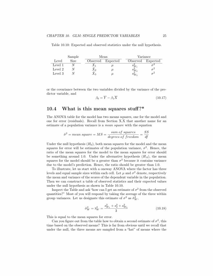
To illustrate, let us start with a oneway ANOVA where the factor has threelevels and equal sample sizes within each cell. Let µ and σ
2 denote, respectivelythe mean and variance of the scores of the dependent variable in the population.Then we can construct a table of observed statistics and their expected valuesunder the null hypothesis as shown in Table 10.10.
Inspect the Table and ask “how can I get an estimate of σ2 from the observedquantities?” Most of you will respond by taking the average of the three withingroup variances. Let us designate this estimate of σ2 as σ
2W ,
σ2W = s
2W =
s2W1
+ s22 + s
2W3
3(10.18)
This is equal to the mean squares for error.Can you figure out from the table how to obtain a second estimate of σ2, this
time based on the observed means? This is far from obvious until we recall thatunder the null, the three means are sampled from a “hat” of means where the
CHAPTER 10. GLM: SINGLE PREDICTOR VARIABLES 26
overall mean is µ and the variance is σ2/N . Hence, the variance of the observed
means (σ2X
) is expected to equal
s2X =
σ2
N(10.19)
where N is the sample size within a group.We can now derive a second estimate of σ2, this time based on the observed
means, asσ2X = Ns
2X (10.20)
In short, we treat the three means as if they were three raw scores, calculatetheir variance and then multiply by the same size within each group.
Now ask, if–again, assuming the null hypothesis–I take the estimate of σ2
based on the means and divide it by the estimate of σ2 based on the within-
group variances, what number should I expect? In algebra, If you answered1.0, then you are very close, but not technically correct. For esoteric reasons,among them that a computed variance cannot be negative, the correct answeris “something close to 1.0.” Denoting this ratio as F0, incorporate this wrinkleand write
H0 : F0 =σ2X
σ2W
≈ 1.0 (10.21)
Read “under the null hypothesis, the F ratio–the estimate of the variance basedon the means divided by the estimate of the variance calculated from the within-group variance–should be within spitting distance of 1.0.” Writing this sameequation in terms of the observed statistics gives
H0 : F0 =Ns
2X
s2W
≈ 1.0 (10.22)
Read “under the null hypothesis, the F ratio–N times the variance of the meansdivided by the average of the within group variances–should be around 1.0.”
By now, you should be attuned to how the “analysis of variance” got itsname. It obtains two estimates of the population variance, σ2, and under thenull hypothesis, both estimates should be approximately equal.
What about the alternative hypothesis? Here, there are real differencesamong the means as well the sampling error from the “hat” of means. Let f
�X�
denote the true variance in the means under the alternative hypothesis. Thenthe expected value for calculating the variance of the observed means should be
E�s2X
�= f
�X�+
σ2
N(10.23)
Multiplying by N gives
E�Ns
2X
�= Nf
�X�+ σ
2 (10.24)
CHAPTER 10. GLM: SINGLE PREDICTOR VARIABLES 27
Placing this quantity in the numerator, the average within-group variancein the denominator and taking expectations gives
HA : FA =Ns
2X
s2W
=Nf
�X�+ σ
2
σ2>> 1.0 (10.25)
You can see how the F ratio under the alternative hypothesis should be “some-thing much greater than 1.0.” (The “much greater than” is relative to the actualdata.)
10.5 Multiple Comparison Procedures*Although R
2 is a measure of effect size in a oneway ANOVA, it suffers from onemajor limitation—it does not indicate which groups may be responsible for asignificant effect. All that a significant R
2 and the F statistic say is that themeans for all groups are unlikely to have been sampled from a single hat ofmeans. Unfortunately, there is no simple, unequivocal statistical solution to theproblem of comparing the means for the different levels of an ANOVA factor.
The fundamental difficulty can be illustrated by imaging a study on per-sonality in which the ANOVA factor was astrological birth sign. There are 12birth signs, so a comparison between the all possible pairs of birth signs wouldresult in 66 different statistical tests. One might be tempted to say that 5%of these tests might be significant by chance, but that statement is misleadingbecause the tests are not statistically independent. The Virgo mean that getscompared to the Leo mean is the same mean involved in, say, the Virgo andPisces comparison.
Because of these problems, a number of statistical methods have been de-veloped to test for the difference in means among the levels of an ANOVAfactor. Collectively, these are known as multiple comparison procedures (MCP)or, sometimes, as post hoc (i.e., “after the fact”) tests , and this very name shouldcaution the user that these tests should be regarded more as an afterthoughtthan a rigorous examination of pre-specified hypotheses.
Opinions about MCPs vary. Many professionals([?]; [?, ?]) advocate usingonly planned or a priori comparisons. Others view them as useful adjunctsto rigorous hypothesis testing. Still others (e.g., [?]) regard some MCPs ashypothesis-generating techniques rather than hypothesis-testing strategies. Ev-eryone, however, agrees on the following: if you have a specific hypothesis onhow the means should differ, never use MCPs to test that hypothesis. You willalmost always be testing that hypothesis with less rigor and statistical powerthan using a planned comparison.
Our first advice on MCP is to avoid them whenever possible. It is not thatthey are wrong or erroneous. Instead, they are poor substitutes for formulatinga clear hypothesis about the group means, coding the levels of the ANOVAfactor to embody that hypothesis, and then directly testing the hypothesis.The proper role for post hoc tests is in completely atheoretical situations wherethe investigator lacks any clear direction about which means might differ from
CHAPTER 10. GLM: SINGLE PREDICTOR VARIABLES 28
which others. Here, they can be useful for detecting unexpected differences thatmay be important for future research.
10.5.1 Traditional multiple comparison proceduresOne problem with MCPs is their availability in different software packages. Notall software supports all MCPs. Hence, we concentrate here on “classic” (read“old”) MCPs that are implemented in the majority of software packages. It isworthwhile consulting the documentation for your own software because modernMCPs have advantages over the older methods.
The traditional MCPs are listed in Table 10.11 along with their applicabil-ity to unbalanced ANOVAs and their general error rates. Note that the entriesin this table, although based on considerable empirical work from statisticians,still involve elements of subjective judgment and oversimplification. For exam-ple, the Student-Newman-Keuls (SNK) procedure can be used with unequal Nprovided that the disparity among sample size is very small. Similarly, SNKcan have a low false positive rate in some circumstances. Also note that sometests can be implemented differently in different software. For example, Fisher’sLeast Significant Differences (LSD) is listed in Table 1.1 as not requiring equalsample sizes. This may not be true in all software packages.
The generic statistical problem with MCP—hinted to above—is that onecan make a large number of comparisons of means and that the probability of afalse positive judgment increases with the number of statistical tests performed.One solution is to perform t tests between every pair of means, but to adjustthe alpha level of the individual t tests so that the overall probability of a falsepositive judgment (i.e., Type I error) is the standard alpha value of .05 (orwhatever value the investigator chooses). This overall probability is sometimescalled the experimentwise, studywise, familywise, or overall error rate. Let αO
denote this overall, studywise alpha and let αI denote the alpha rate for anindividual statistical test. Usually, the goal to to set αO to some value andthen, with some assumptions, derive αI .
Two corrections, the Bonferroni and Sidak entries in Table 10.11 . Thesimpler of the two correction is the Bonferroni (aka Bonferroni-Dunn). If thereare k levels to a GLM factor, then the number of pairwise mean comparisonswill be
c =k(k − 1)
2(10.26)
A Bonferroni calculates αI as αO/c or the overall alpha divided by the numberof comparisons. If there are four levels to a GLM factor, then c = 6 and with anoverall αO set to .05, αI = .05/6= .0083. Hence, a a test between any two meansmust have a significance level of .0083 or greater before it is called significant.
A second approach is to recognize that the probability of a making at leastone false positive (or Type I error) in two completely independent statisticaltests is
1−�1− αI
2�= 1− .95
2= .0975 (10.27)

CHAPTER 10. GLM: SINGLE PREDICTOR VARIABLES 29
Tabl
e10
.11:
Trad
itio
nalm
ulti
ple
com
pari
son
test
s.
Pro
cedu
reE
qual
sam
ple
size
?
Fals
epo
sitive
rate
Fals
ene
gative
rate
Com
men
tsB
onfe
rron
i1N
oLo
wH
igh
Adj
usts
αle
vel
Šidá
kN
oLo
wH
igh
Adj
usts
αle
vel
Fish
er’s
LSD
2N
oH
igh
Low
Mos
tlib
eral
Dun
can
MRT
3Y
esM
oder
ate
Mod
erat
eN
otw
idel
yre
com
men
ded
SNK
4Y
esM
oder
ate
Mod
erat
eH
ochb
erg
(GT
2)N
oLo
wM
oder
ate
Tuke
y5N
oLo
wM
oder
ate
Mor
epo
wer
ful
than
GT
2Sc
heffè
No
Low
Hig
hM
ost
cons
verv
ativ
e
Dun
nett
No
Low
Hig
hC
ompa
riso
nw
ith
are
fere
nce
grou
p1
Als
oca
lled
Bon
ferr
oni-D
unn;
2LS
D=
leas
tsi
gnifi
cant
diffe
renc
es;s
omet
imes
calle
dSt
uden
t’s
T;
3M
RT=
mul
tipl
era
nge
test
;4
SNK
=St
uden
t-N
ewm
an-K
euls
test
;5
also
calle
dH
SD=
hone
stsi
gnifi
cant
diffe
renc
esan
dTu
key-
Kra
mer
insp
ecifi
csi
tuat
ions
.
CHAPTER 10. GLM: SINGLE PREDICTOR VARIABLES 30
when αI = .05. In general, and the overall studywise alpha (αO) for c indepen-dent comparisons is
αO = 1− (1− αI)c (10.28)
Setting αO to a specified level and solving for αI gives
αI = 1− (1− αO)1/c (10.29)
This is [?]Šidák’s (1967) MCP.A key assumption to the Bonferroni and Sidak correlations is that all the
tests are statistically independent. This is clearly false but the extent to whichit compromises the test is not well understood. Another MCP strategy is toignore the independent-dependent issue altogether and compute t tests for everypair of means using the traditional αI . This approach is embodied in whathas become to be known as Fisher’s Least-Significant-Differences (LSD), Fisherclaimed that these tests were valid as long as the overall F for the ANOVAfactor was significant, in which case the test has been termed Fisher’s ProtectedLeast-Significant Differences or PLSD. (Many statisticians dispute this claim).The LSD and PLSD are liberal tests. That is, they are prone to false positive(Type I) errors.
Because Fisher’s PLSD and the Sidak and Bonferroni corrections are basedon t tests, they require the typical assumptions of the t test—normal distribu-tions within groups and homogeneity of variance. Scheffè’s test, another MCP,does not require these assumptions, and hence gained popularity before otherrobust MCPs were developed. Scheffè’s test will not give a significant pairwisecomparison unless the overall F for the ANOVA factor is significant. The test,however, is conservative. That is, it minimizes false positives, but increases theprobability of a false negative inference (Type II error).
Except for Dunnett’s test, the remaining procedures listed in Table 10.11vary in their error rates between the liberal LSD and the conservative Scheffè.Duncan’s Multiple Range Test (MRT) is widely available, but many statisticiansrecommend that it not be used because it has a high false positive rate. TheStudent-Newman-Keul’s procedure (SNK) is widely used because it originated inthe earlier part of the 20th century and underwent development into the 1950s.It should not be used with strongly unbalanced data. The Tukey-Kramer MCP(also called Tukey or Tukey-Kramer honestly significant differences) is anotherintermediate test that can be used with unbalanced designs. It is preferred toits nearest method, Hochberg’s GT2, because it is slightly more powerful.
Dunnett’s test deserved special mention. This test is designed to comparethe mean of each treatment group against a control mean. Hence, it may be theMCP of choice for some studies.