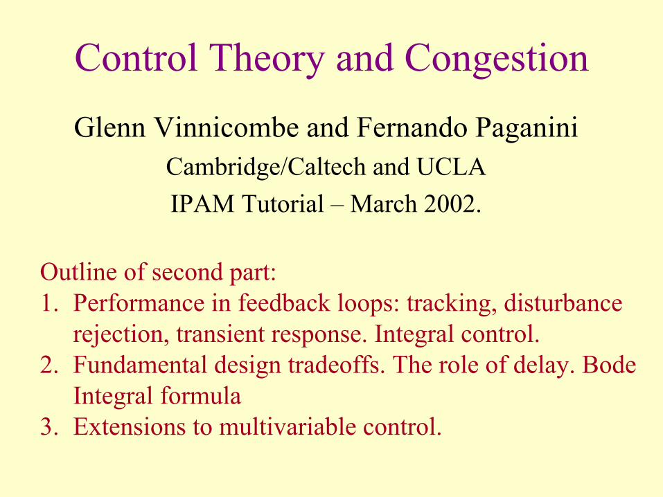
Control Theory and CongestionGlenn Vinnicombe and Fernando Paganini

Cambridge/Caltech and UCLAIPAM Tutorial – March 2002.

Outline of second part:1. Performance in feedback loops: tracking, disturbance

rejection, transient response. Integral control.2. Fundamental design tradeoffs. The role of delay. Bode

Integral formula3. Extensions to multivariable control.

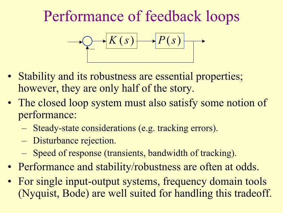
Performance of feedback loops

• Stability and its robustness are essential properties; however, they are only half of the story.

• The closed loop system must also satisfy some notion of performance:– Steady-state considerations (e.g. tracking errors).– Disturbance rejection.– Speed of response (transients, bandwidth of tracking).

• Performance and stability/robustness are often at odds.• For single input-output systems, frequency domain tools

(Nyquist, Bode) are well suited for handling this tradeoff.

( )P s( )K s

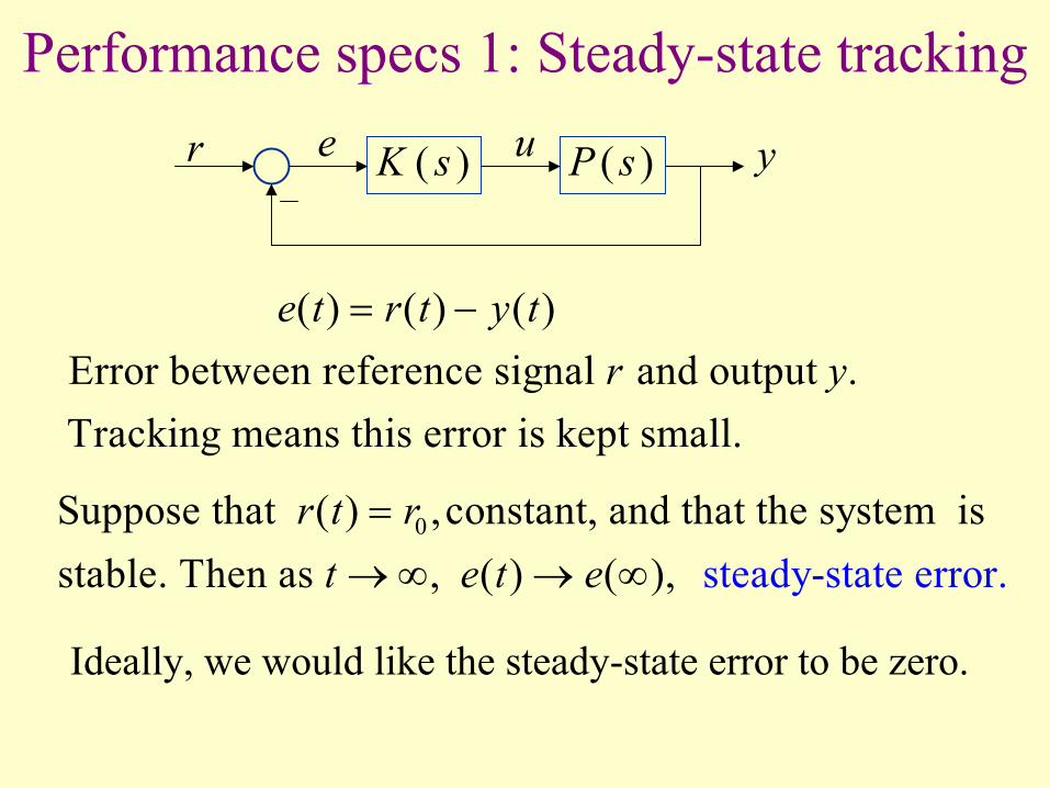
Performance specs 1: Steady-state tracking

( ) ( ) ( )Error between reference signal and output .Tracking means this error is kept small.

e t r t y tr y

= −

0Suppose that ( ) ,constant, and that the system is stable. Then as , ( ) stea( ), dy-state error.

r t rt e t e=→ ∞ → ∞

Ideally, we would like the steady-state error to be zero.

( )P s( )K s u yr e

Tracking, sensitivity and loop gain

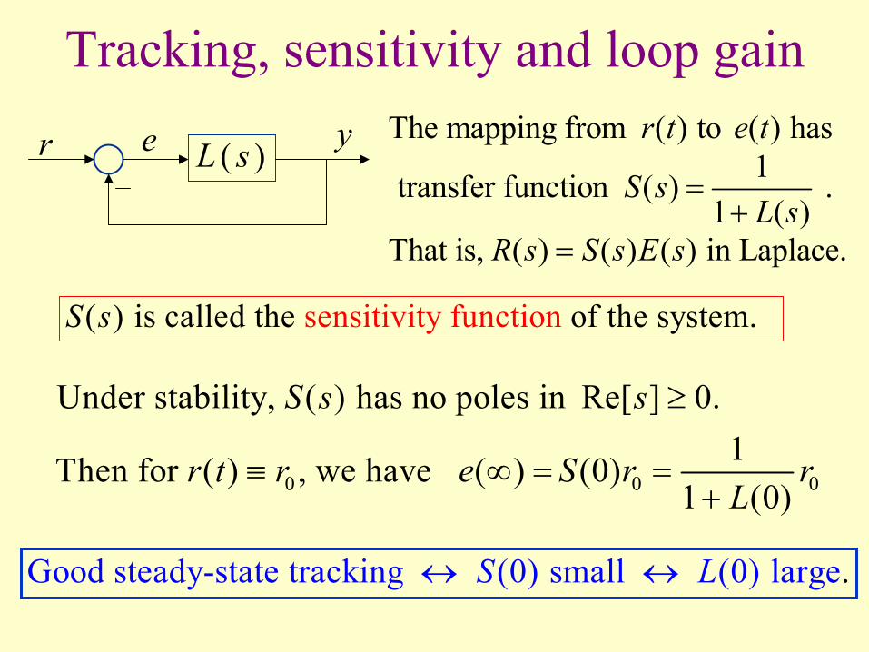
( )L s yr e The mapping from ( ) to ( ) has1transfer function ( ) .

1 ( )That is, ( ) ( ) ( ) in Laplace.

r t e t

S sL s

R s S s E s

=+

=

0 0 0

Under stability, ( ) has no poles in Re[ ] 0.1Then for ( ) , we have ( ) (0)

1 (0)

S s s

r t r e S r rL

≥

≡ ∞ = =+

Good steady-state tracking (0) small (0) l .argeS L↔ ↔

sensitivity function( ) is called the of the system. S s

Integral control

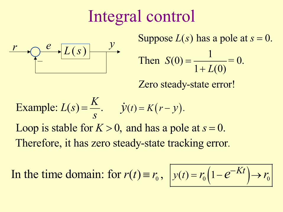
( )L s yr eSuppose ( ) has a pole at 0.

1Then (0) = 0. 1 (0)

Zero steady-state error!

L s s

SL

=

=+

( )( ) .

.

Example: ( ) .

Loop is stable for 0, and has a pole at 0.Therefore, it has zero steady-state tracking error

t K rKL s ysK s

y = −=

> =

( )0 0 0( ) 1In the time domain: for ( ) , Kty tr t r r re−= − →≡

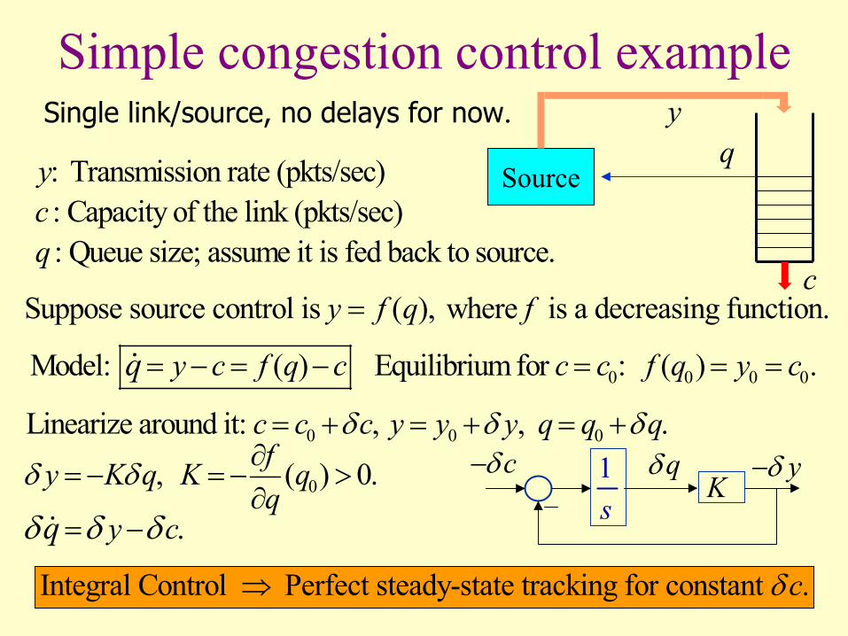
Simple congestion control exampleSingle link/source, no delays for now.

: Transmission rate (pkts/sec): Capacity of the link (pkts/sec): Queue size; assume it is fed back to source.

ycq

Source

yq

cSuppose source control is ( ), where is a decreasing function.y f q f=

0 0 0 0Model: ( ) Equilibrium for : ( ) .y c f q c c c f q y cq = − = − = = =

0 0 0

0

Linearize around it: , , .

, ( ) 0.

.

c c c y y y q q qfy K q K qq

y cq

δ δ δ

δ δ

δ δ δ

= + = + = +∂

= − = − >∂

= −K

1s

qδcδ− yδ−

Integral Control Perfect steady-state tracking for constant .cδ⇒

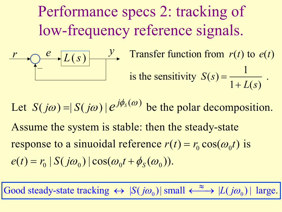
Performance specs 2: tracking of low-frequency reference signals.

( )L s yr e Transfer function from ( ) to ( ) 1is the sensitivity ( ) .

1 ( )

r t e t

S sL s

=+

0 0

0 0 0 0

Assume the system is stable: then the steady-state response to a sinuoidal reference ( ) cos( ) is ( ) | ( ) | cos( ( )).S

r t r te t r S j t

ωω ω φ ω

== +

( )Let ( ) | ( ) | be the polar decomposition.SjS j S j e φ ωω ω=

0 0Good steady-state tracking | ( ) | small | ( ) .| largeS j L jω ω≈↔ ←→

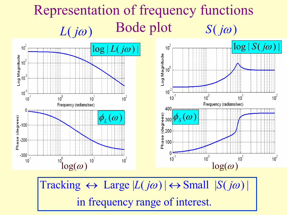
( )L jω ( )S jω

Tracking Large | ( ) | Small | ( ) | in frequency range of interest.

L j S jω ω↔ ↔

log | ( ) |L jω log | ( ) |S jω

( )Lφ ω ( )Sφ ω

Representation of frequency functions Bode plot

log( )ω log( )ω

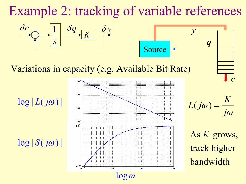
Example 2: tracking of variable references

Source

yq

c

K1s

qδcδ− yδ−

log | ( ) |L jω

log | ( ) |S jω

logω

( ) KL jj

ωω

=

As grows, track higherbandwidth

K

Variations in capacity (e.g. Available Bit Rate)

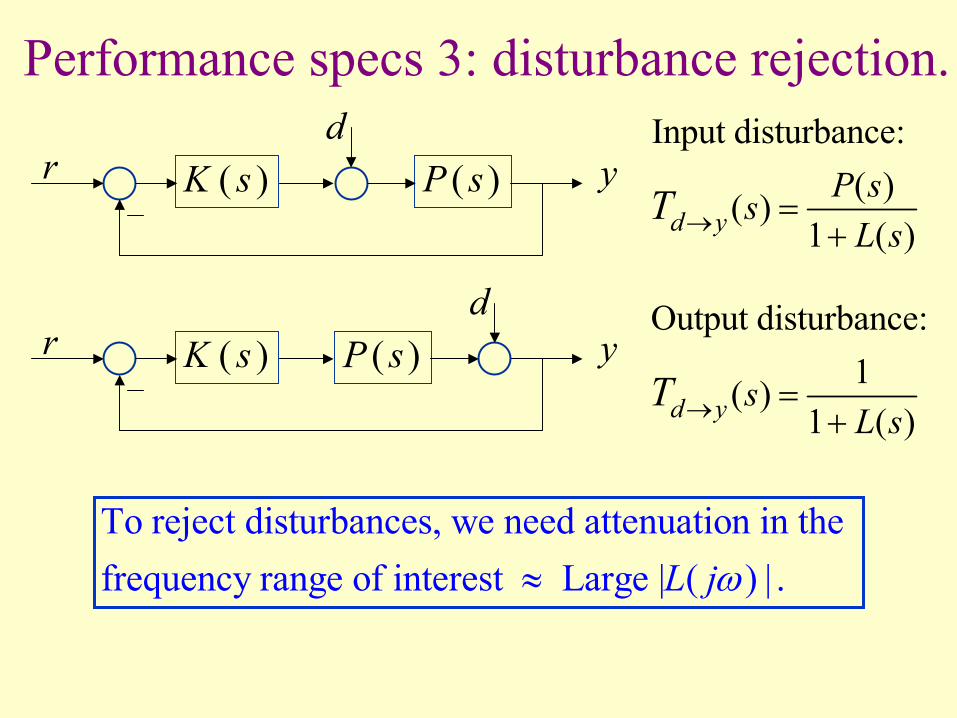
Performance specs 3: disturbance rejection.

( )P s( )K s yrd

( )P s( )K s yrd

Input disturbance:( )( )

1 ( )d yP ssL s

T → =+

Output disturbance:1( )

1 ( )d y s L sT → =

+

To reject disturbances, we need attenuation in the frequency range of interest Large | ( ) | .L jω≈

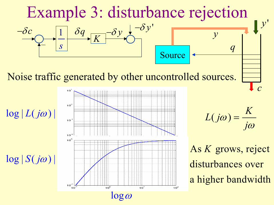
Example 3: disturbance rejection

Source

yq

c

K1s

qδcδ− yδ−

log | ( ) |L jω

log | ( ) |S jω

logω

( ) KL jj

ωω

=

As grows, reject disturbances over a higher bandwidth

K

Noise traffic generated by other uncontrolled sources.

'y'yδ−

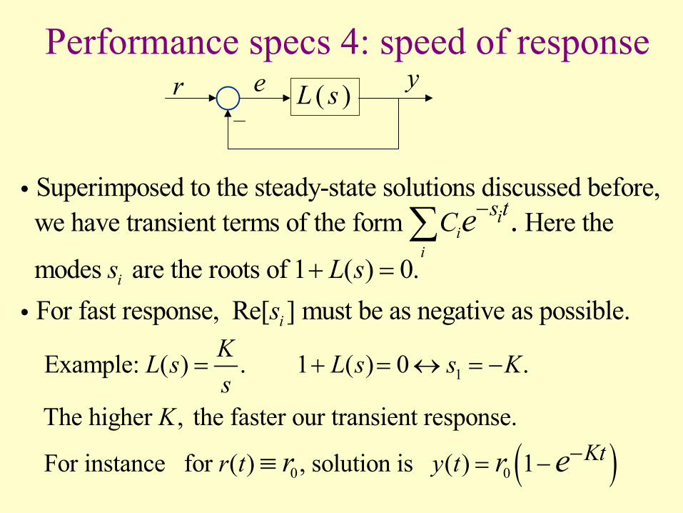
Performance specs 4: speed of response

Superimposed to the steady-state solutions discussed before, we have transient terms of the form Here the

modes are the roots of 1 ( ) 0. For fast response, Re[ ] must be as ne

.ii

i

i

is tC

s L ss

e−

+ =∑

i

i gative as possible.

1Example: ( ) . 1 ( ) 0 .

The higher , the faster our transient response.

KL s L s s Ks

K

= + = ↔ = −

( )0 0For instance for ( ) , solution is ( ) 1 Ktr t y tr r e−= −≡

( )L s yr e

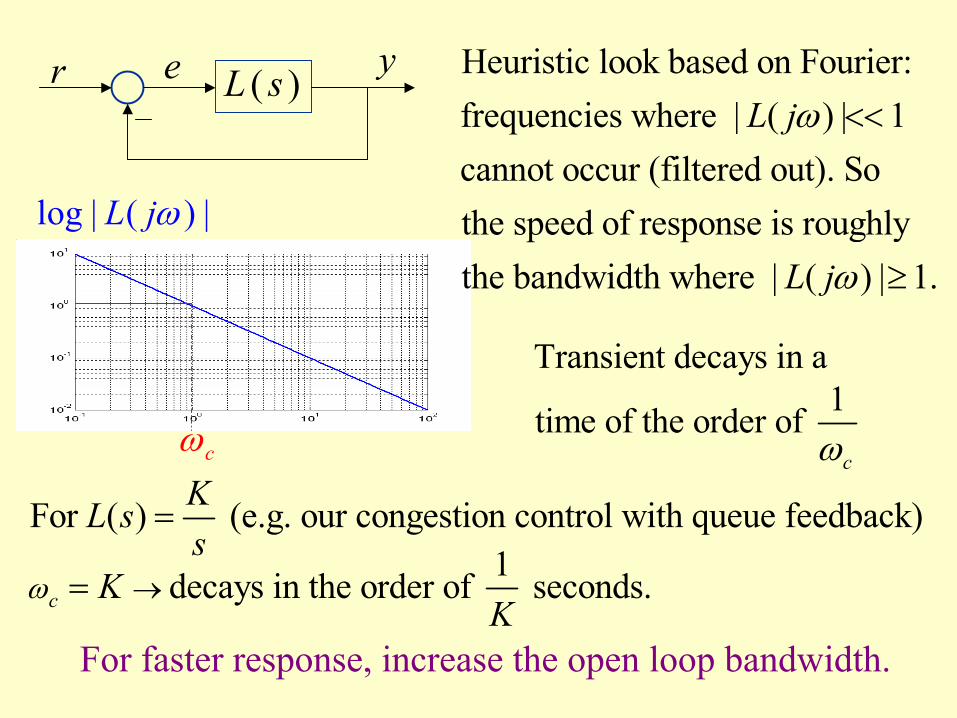
( )L s yr e

log | ( ) |L jω

cω

Transient decays in a 1time of the order of cω

For ( ) (e.g. our congestion control with queue feedback)1decays in the order of seconds.c

KL ss

KK

ω →

=

=

For faster response, increase the open loop bandwidth.

Heuristic look based on Fourier: frequencies where | ( ) | 1 cannot occur (filtered out). So the speed of response is roughlythe bandwidth where | ( ) | 1.

L j

L j

ω

ω

<<

≥

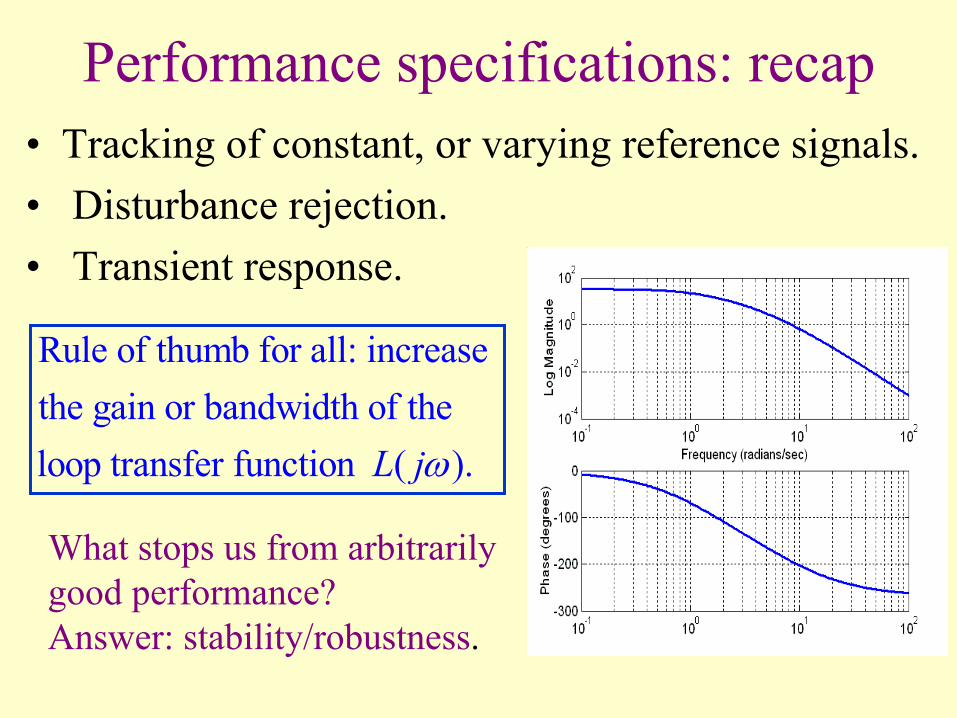
Performance specifications: recap• Tracking of constant, or varying reference signals. • Disturbance rejection.• Transient response.

Rule of thumb for all: increase the gain or bandwidth of the loop transfer function ( ).L jω

What stops us from arbitrarilygood performance?Answer: stability/robustness.

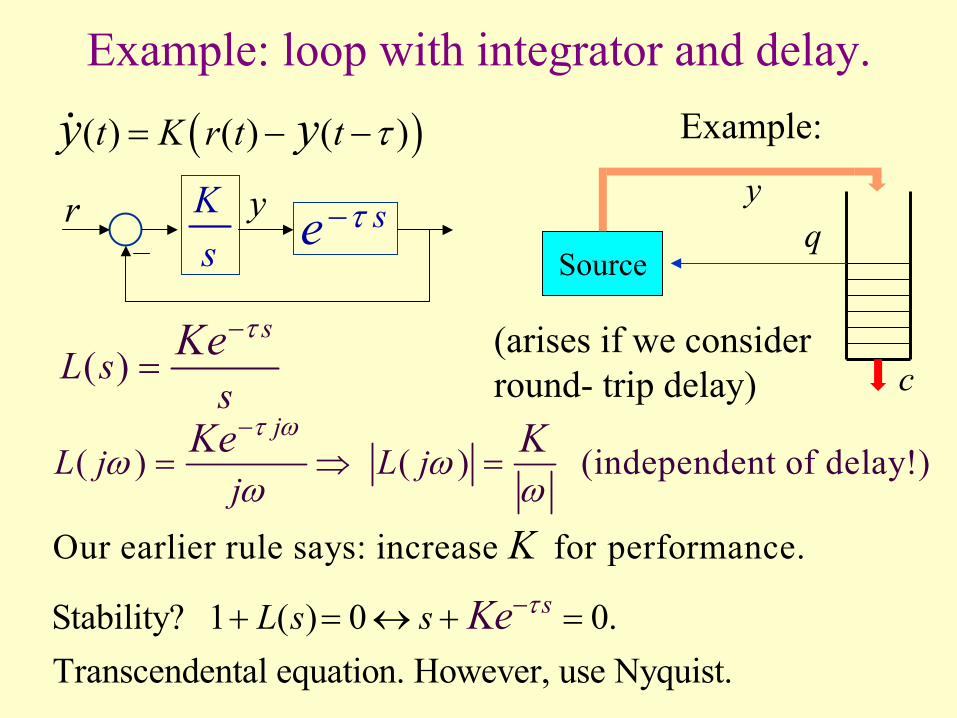
Example: loop with integrator and delay.

( )( ) ( ) ( )t K r t ty y τ= − −

se τ−Ksyr

( )s

L ss

Ke τ−=

Our

( ) ( ) (independent of d

earlier rule says: increase for pe

el

rformance.

ay!)

jL j L j

jK

Ke Kτ ωω ω

ω ω

−= ⇒ =

Stability? 1 ( ) 0 0.Transcendental equation. However, use Nyquist.

sL s s Ke τ−+ = ↔ + =

Source

yq

c(arises if we consider round- trip delay)

Example:

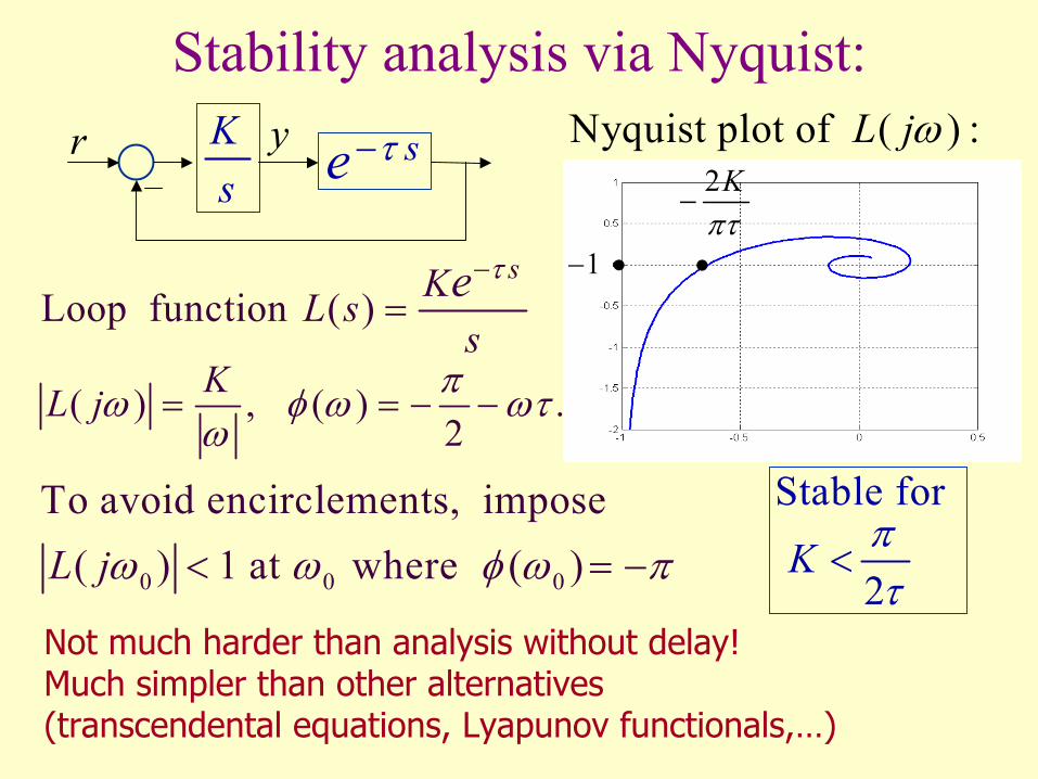
Stability analysis via Nyquist:

Loop function ( )sKL s

se τ−

=

( ) , ( ) .2

KL j πω φ ω ωτω

= = − −

0 0 0

To avoid encirclements, impose ( ) 1 at where ( )L jω ω φ ω π< = −

2Kπτ

−

•1− •

Nyquist plot of ( ) :L jω

Stable for

2K π

τ<

Not much harder than analysis without delay! Much simpler than other alternatives (transcendental equations, Lyapunov functionals,…)

se τ−Ksyr

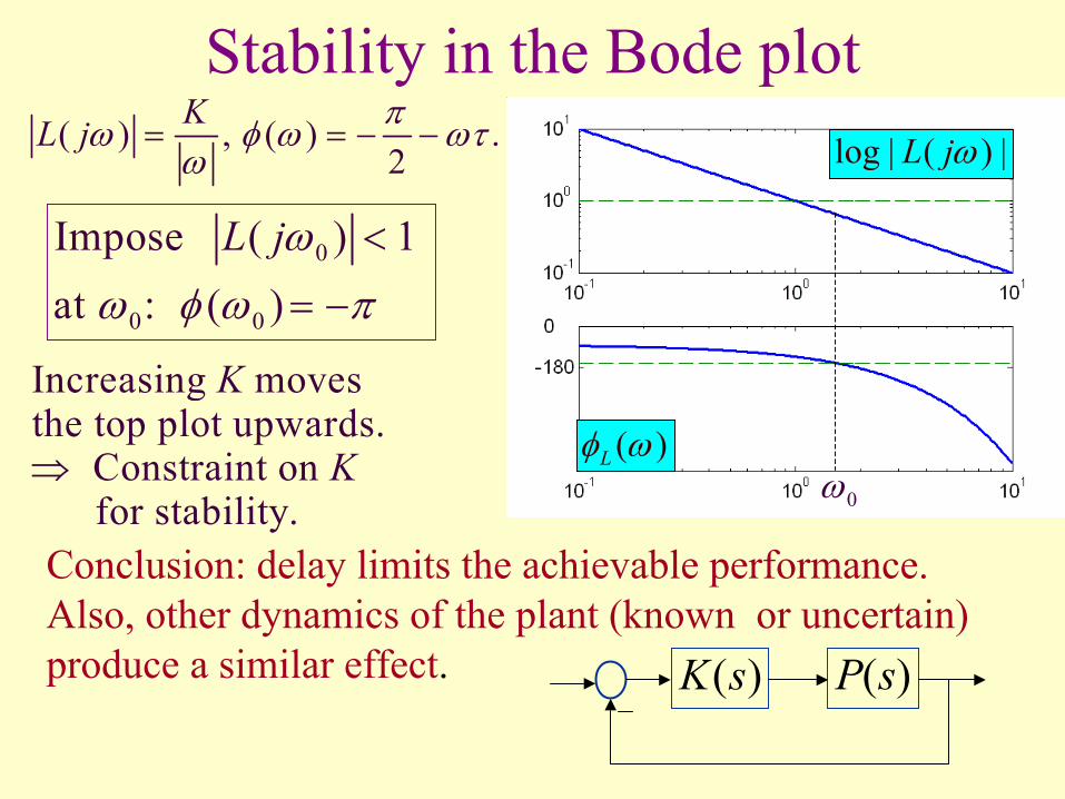
Stability in the Bode plot

0

0 0

Impose ( ) 1 at : ( )

L jωω φ ω π

<

= −

Conclusion: delay limits the achievable performance. Also, other dynamics of the plant (known or uncertain) produce a similar effect. ( )P s( )K s

log | ( ) |L jω

( )Lφ ω0ω

( ) , ( ) .2

KL j πω φ ω ωτω

= = − −

Increasing moves the top plot upwards.

Constraint on for stability.

K

K⇒

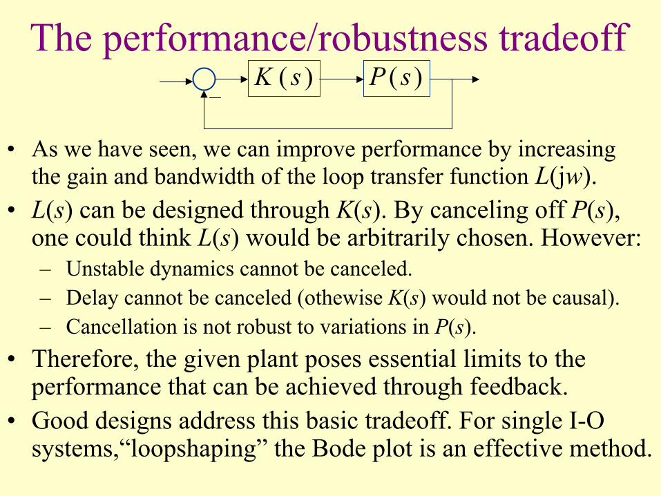
The performance/robustness tradeoff

• As we have seen, we can improve performance by increasing the gain and bandwidth of the loop transfer function L(jw).

• L(s) can be designed through K(s). By canceling off P(s), one could think L(s) would be arbitrarily chosen. However:– Unstable dynamics cannot be canceled.– Delay cannot be canceled (othewise K(s) would not be causal). – Cancellation is not robust to variations in P(s).

• Therefore, the given plant poses essential limits to the performance that can be achieved through feedback.

• Good designs address this basic tradeoff. For single I-O systems,“loopshaping” the Bode plot is an effective method.

( )P s( )K s

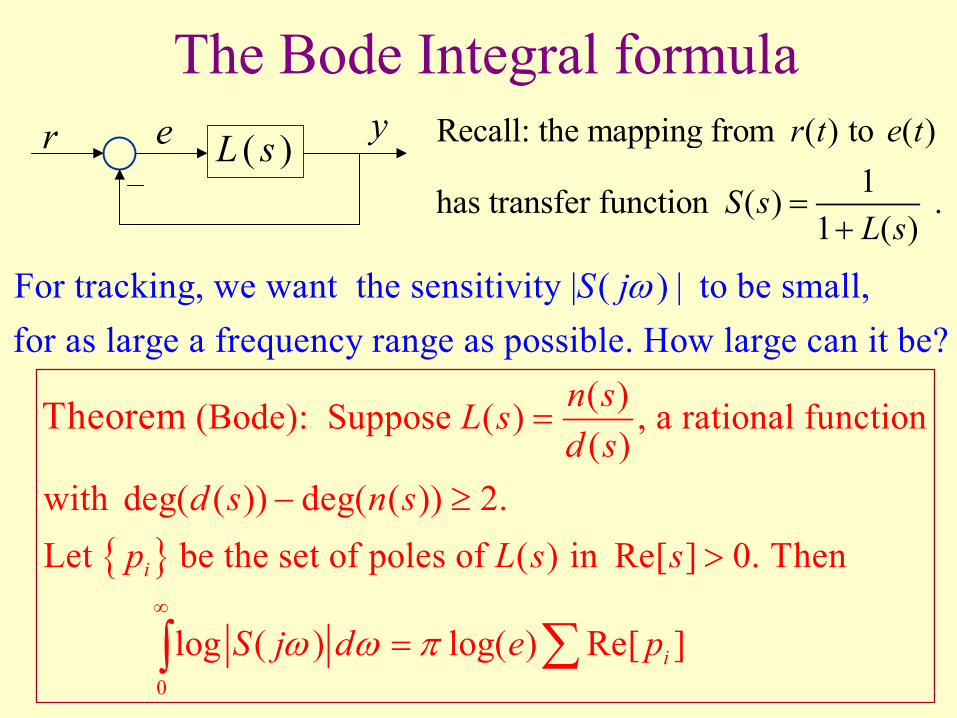
The Bode Integral formula ( )L s yr e Recall: the mapping from ( ) to ( )

1has transfer function ( ) . 1 ( )

r t e t

S sL s

=+

For tracking, we want the sensitivity | ( ) | to be small, for as large a frequency range as possible. How large can it be?

S jω

{ }

0

( ) (Bode): Suppose ( ) , a rational function( )

with deg( ( )) deg( ( )) 2. Let be the set of poles of ( ) in Re[ ] 0. Then

log ( ) log( ) Re[ ]

Theorem

i

i

n sL sd s

d s n sp L s s

S j d e pω ω π∞

=

− ≥

>

= ∑∫

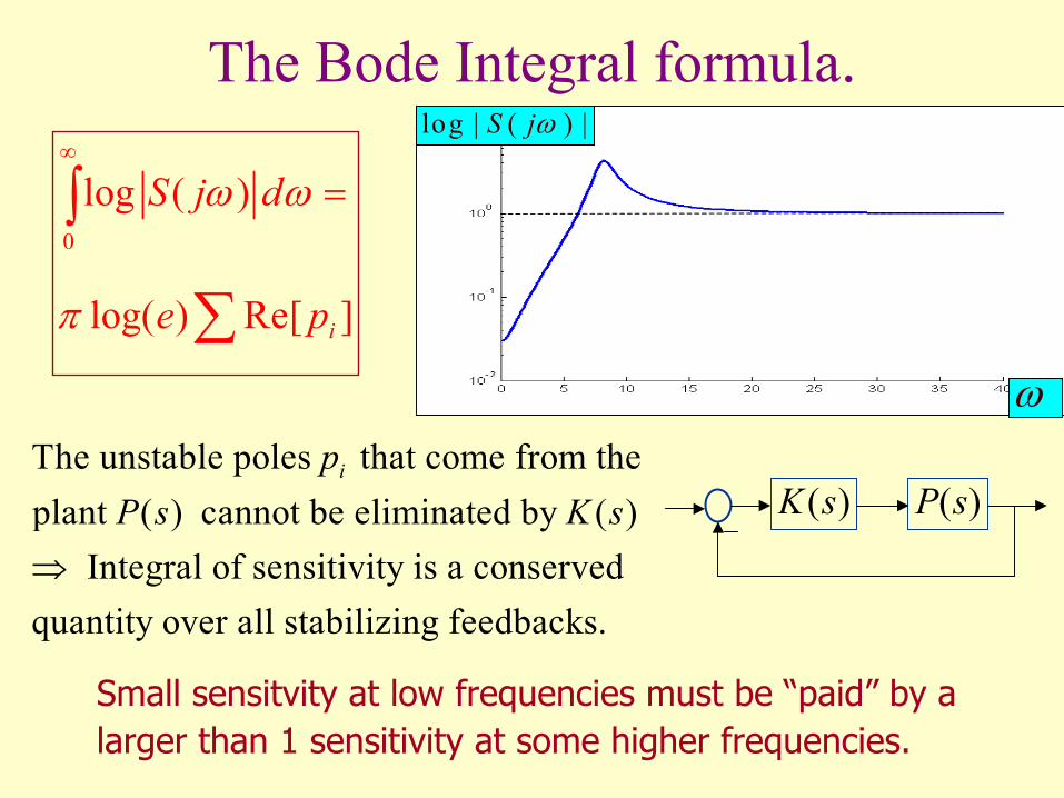
The Bode Integral formula.

0

log ( )

log( ) Re[ ]i

S j d

e p

ω ω

π

∞

=∫

∑

log | ( ) |S jω

ω

( )P s( )K sThe unstable poles that come from theplant ( ) cannot be eliminated by ( )

Integral of sensitivity is a conserved quantity over all stabilizing feedbacks.

ipP s K s

⇒

Small sensitvity at low frequencies must be “paid” by alarger than 1 sensitivity at some higher frequencies.

But all this is only linear!• The above tradeoff is of course present in nonlinear

systems, but harder to characterize, due to the lack of a frequency domain (partial extensions exist).

• So most successful designs are linear based, followed up by nonlinear analysis or simulation.

• Beware of claims of superiority of “truly nonlinear” designs. They rarely address this tradeoff, so may have poor performance or poor robustness (or both).

• A basic test: linearized around equilibrium, the nonlinear controller should not be worse than a linear design.

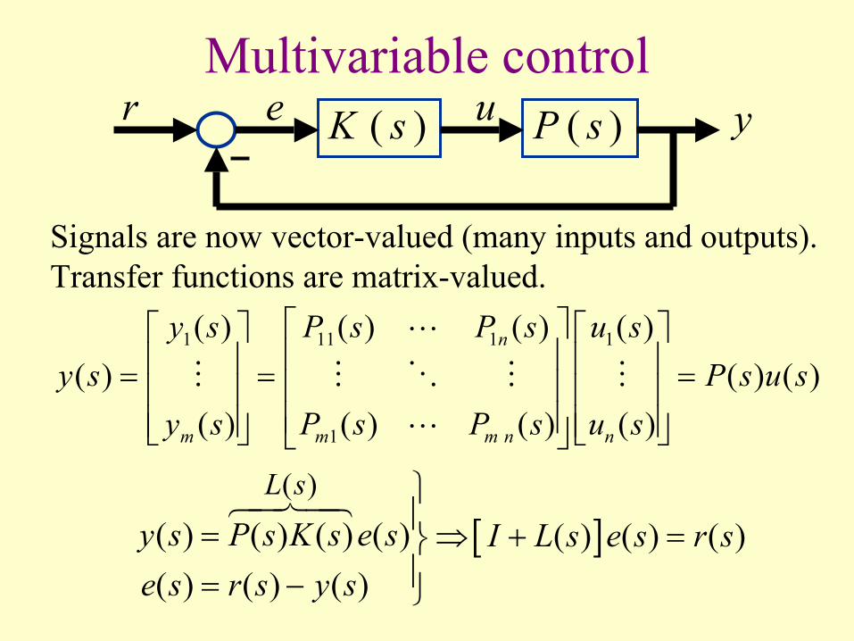
Multivariable control( )P s( )K s u yr e

Signals are now vector-valued (many inputs and outputs).Transfer functions are matrix-valued.

1 11 1 1

1

( ) ( ) ( ) ( )( ) ( ) ( )

( ) ( ) ( ) ( )

n

m m m n n

y s P s P s u sy s P s u s

y s P s P s u s

= = =

[ ]( )

( ) ( ) ( ) ( ) ( ) ( ) ( )( ) ( ) ( )

L s

y s P s K s e s I L s e s r se s r s y s

= ⇒ + == −

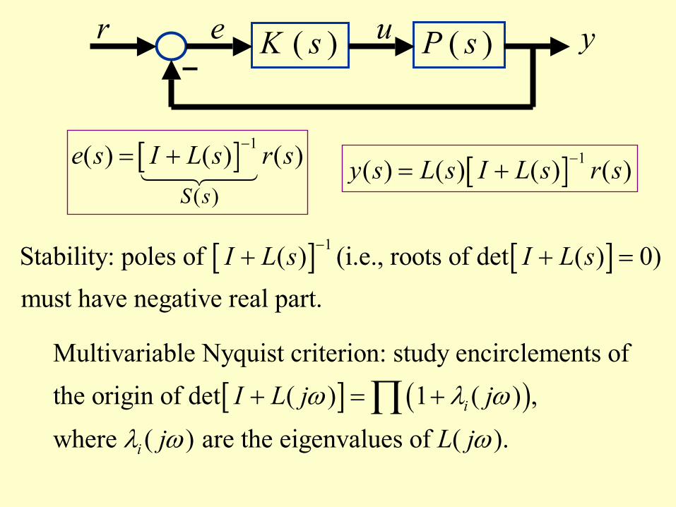
[ ] 1

( )

( ) ( ) ( )S s

e s I L s r s−= +

( )P s( )K s u yr e

[ ] 1( ) ( ) ( ) ( )y s L s I L s r s−= +

[ ] [ ]1Stability: poles of ( ) (i.e., roots of det ( ) 0)must have negative real part.

I L s I L s−+ + =

[ ] ( )Multivariable Nyquist criterion: study encirclements ofthe origin of det ( ) 1 ( ) ,

where ( ) are the eigenvalues of ( ).i

i

I L j j

j L j

ω λ ω

λ ω ω

+ = +∏

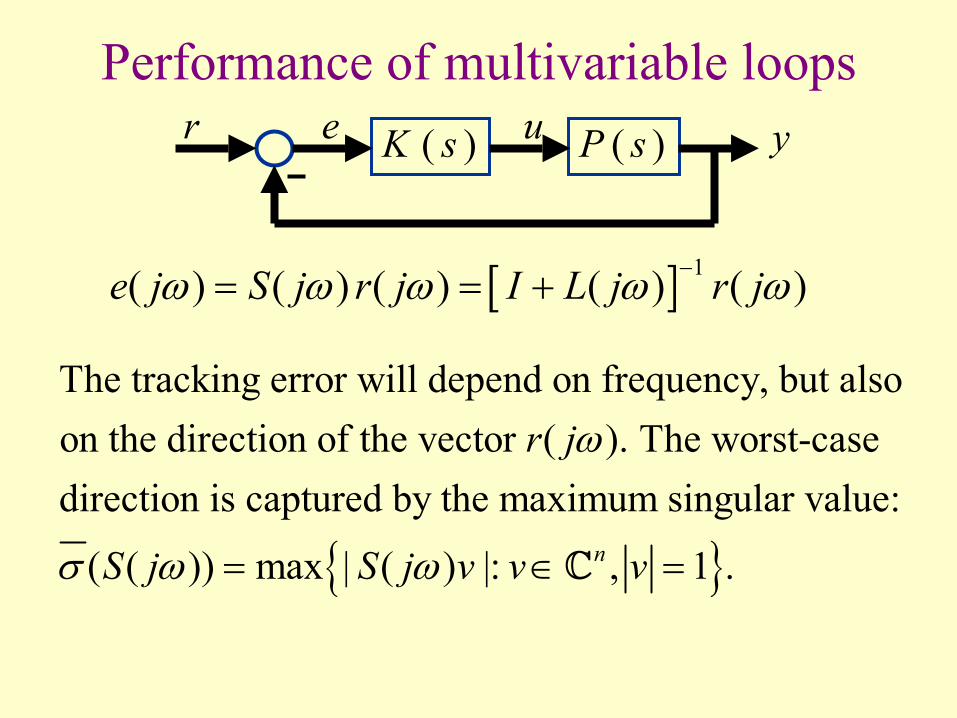
Performance of multivariable loops( )P s( )K s u yr e

[ ] 1( ) ( ) ( ) ( ) ( )e j S j r j I L j r jω ω ω ω ω−= = +

{ }

The tracking error will depend on frequency, but alsoon the direction of the vector ( ). The worst-casedirection is captured by the maximum singular value:

( ( )) max | ( ) |: , 1 .n

r j

S j S j v v v

ω

σ ω ω= ∈ =C

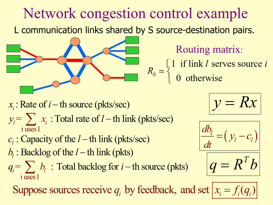
Network congestion control exampleL communication links shared by S source-destination pairs.

1 if link serves source 0 otherwise li

l iR

=

Routing matrix:

i uses l

i uses l

: Rate of th source (pkts/sec): Total rate of th link (pkts/sec)

: Capacity of the th link (pkts/sec): Backlog of the th link (pkts)

: Total backl

=

og for s= th

i

l

l

l

i

li

x iy l

c

x

lb lq ib

−−

−−

−

∑

∑ ource (pkts)

y Rx=

( )ll l

dbdt

y c= −

Tq R b=

Suppose sources receive by feedback, and set ( )i i i iq x f q=

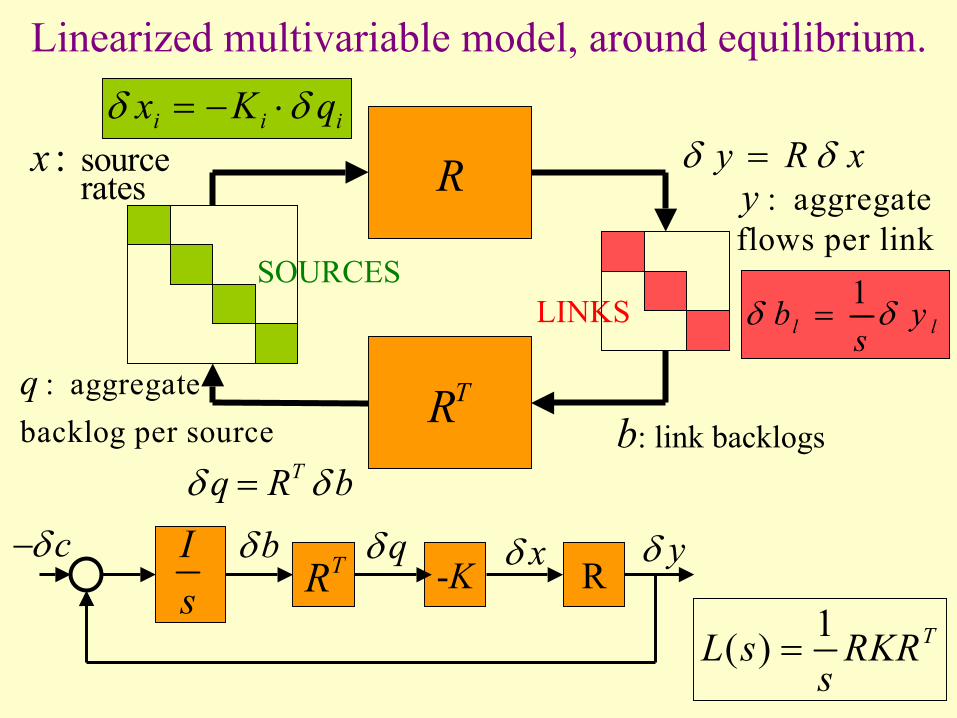
Linearized multivariable model, around equilibrium.

LINKSSOURCES

R

TR

source rates

:x: aggregate

flows per linky

: aggregate backlog per sourceq

b: link backlogs

y R xδ δ=

Tq R bδ δ=

i i ix K qδ δ= − ⋅

1l lb y

sδ δ=

R-KIs

TRbδ qδ xδ yδcδ−

1( ) TL s RKRs

=

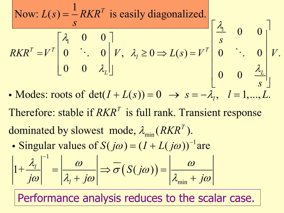
1Now: ( ) is easily diagonalized.TL s RKRs

=

, 0 ( ) .T T Tl

L L

sRKR V V L s V V

s

λλ

λλ λ

1

1

0 0 0 0 = 0 0 ≥ ⇒ = 0 0 0 0 0 0

min

Modes: roots of det( ( )) 0 , 1,..., .

Therefore: stable if is full rank. Transient response dominated by slowest mode, ( ).

lT

T

I L s s l L

RKRRKR

λ

λ

+ = → = − =i

( )

1

1

min

Singular values of ( ( ( )) are

1+ (l

l

S j I L j

S jj j j

ω ωλ ω ωσ ωω λ ω λ ω

−

−) = +

= ⇒ ) =+ +

i

Performance analysis reduces to the scalar case.

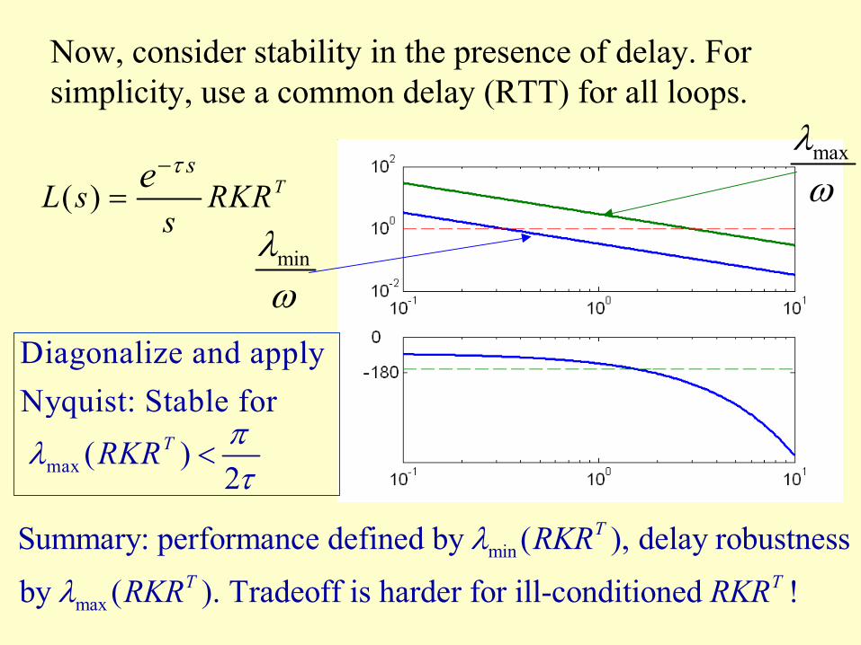
( ) Ts

L s RKRse τ−

=

Now, consider stability in the presence of delay. For simplicity, use a common delay (RTT) for all loops.

minλω

maxλω

max

Diagonalize and apply Nyquist: Stable for ( )

2TRKR πλ

τ<

min

max

Summary: performance defined by ( ), delay robustness

by ( ). Tradeoff is harder for ill-conditioned !

T

T T

RKR

RKR RKR

λ

λ

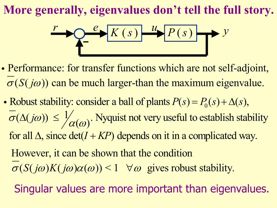
More generally, eigenvalues don’t tell the full story.

( )P s( )K s u yr e

Performance: for transfer functions which are not self-adjoint,( ( )) can be much larger-than the maximum eigenvalue.S jσ ω

i

0 Robust stability: consider a ball of plants ( ) ( ) ( ),1( ( )) . Nyquist not very useful to establish stability ( )

for all , since det( ) depends on it in a complicated way.

P s P s sj

I KP

σ ω α ω

= +∆∆ ≤

∆ +

i

However, it can be shown that the condition ( ( ) ( ) ( )) < 1 gives robust stability.S j K jσ ω ω α ω ω∀

Singular values are more important than eigenvalues.

Summary• A well designed feedback will respond as quickly as possible to

regulate, track references or reject disturbances.• The fundamental limit to the above features is the potential for

instability, and its sensitivity to errors in the model. A good design must balance this tradeoff (robust performance).

• In SISO, linear case, tradeoff is well understood by frequency domain methods. This explains their prevalence in design.

• Nonlinear aspects usually handled a posteriori. Nonlinear control can potentially (but not necessarily) do better. A basic test: linearizationaround any operating point should match up with linear designs.

• In multivariable systems, frequency domain tools extend with some complications (ill conditioning, singular values versus eigenvalues,…)

• All of this is relevant to network flow control: performance vs delay/robustness, ill-conditioning,… Nonlinearity seems mild.