Embed Size (px)
Citation preview

GIS and Cartography at the University of Toronto Technical Paper Series - Paper no. 3
GCUT - GIS and Cartography at the University of Toronto Technical Paper Series University of Toronto, Department of Geography and Program in Planning
This series is published as a technical complement to research projects undertaken in the Department of Geography and Program in Planning. These projects are related to research by Geography Department faculty or other university collaborators. The series was initiated to document and disseminate innovative methods in GIS (Geographic Information Systems) and Cartography which have been developed for these projects. It allows these methods to be described in detail for the purposes of review and replication, and to be referenced concisely by papers in academic journals or other publications. This series is intended to encourage the sharing of research methods, and to avoid duplication of effort. This series will be published online in Acrobat Portable Document Format (PDF) for download, accessible through the website of the Department of Geography and Program in Planning: http://www.geog.utoronto.ca/research/publications/gcut
The Authors
Byron Moldofsky, Manager, The Cartography Office, Department of Geography Justin Ngan, Research Assistant, The Cartography Office, Department of Geography, University of Toronto Dr. Angela Colantonio, Associate Professor of Occupational Science and Occupational Therapy, University of Toronto, Senior Research Scientist, Toronto Rehabilitation Institute. The Cartography Office
The mandate of the Cartography Office is to provide mapping and GIS support for teaching and research in the Department of Geography and Program in Planning.
The Toronto Rehabilitation Institute
Dr. Angela Colantonio is an Associate Professor at the University of Toronto, and a Senior Research Scientist at the Toronto Rehabilitation Institute, where she holds the Saunderson Family Chair in Acquired Brain Injury Research. The Toronto Rehabilitation Institute partners with individuals, their families and supporting communities in innovative, effective adult rehabilitation, complex continuing care and long-term care. In affiliation with the University of Toronto, they lead the integration of service, research and education, and the development of a coordinated rehabilitation system. Website: www.torontorehab.on.ca © 2007 University of Toronto Reproduction of maps or tables within this publication requires express written permission of the Department of Geography, University of Toronto. ISSN 1915-2159
2
GIS and Cartography at the University of Toronto Technical Paper Series - Paper no. 3
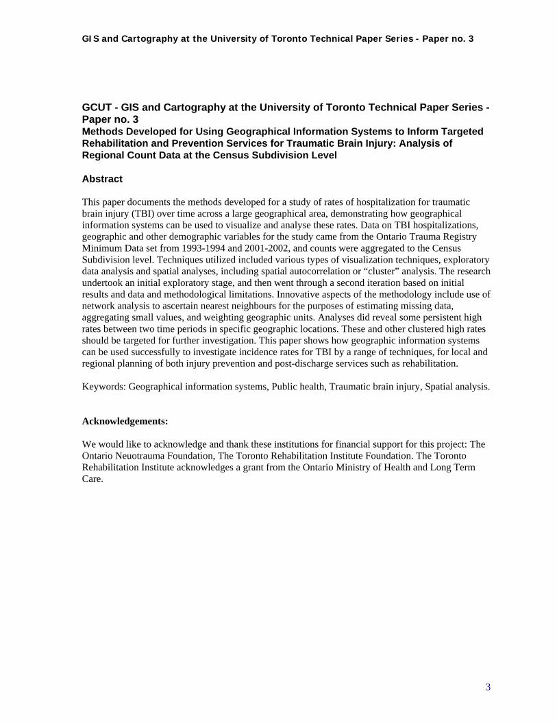
GCUT - GIS and Cartography at the University of Toronto Technical Paper Series - Paper no. 3 Methods Developed for Using Geographical Information Systems to Inform Targeted Rehabilitation and Prevention Services for Traumatic Brain Injury: Analysis of Regional Count Data at the Census Subdivision Level Abstract This paper documents the methods developed for a study of rates of hospitalization for traumatic brain injury (TBI) over time across a large geographical area, demonstrating how geographical information systems can be used to visualize and analyse these rates. Data on TBI hospitalizations, geographic and other demographic variables for the study came from the Ontario Trauma Registry Minimum Data set from 1993-1994 and 2001-2002, and counts were aggregated to the Census Subdivision level. Techniques utilized included various types of visualization techniques, exploratory data analysis and spatial analyses, including spatial autocorrelation or “cluster” analysis. The research undertook an initial exploratory stage, and then went through a second iteration based on initial results and data and methodological limitations. Innovative aspects of the methodology include use of network analysis to ascertain nearest neighbours for the purposes of estimating missing data, aggregating small values, and weighting geographic units. Analyses did reveal some persistent high rates between two time periods in specific geographic locations. These and other clustered high rates should be targeted for further investigation. This paper shows how geographic information systems can be used successfully to investigate incidence rates for TBI by a range of techniques, for local and regional planning of both injury prevention and post-discharge services such as rehabilitation. Keywords: Geographical information systems, Public health, Traumatic brain injury, Spatial analysis. Acknowledgements: We would like to acknowledge and thank these institutions for financial support for this project: The Ontario Neuotrauma Foundation, The Toronto Rehabilitation Institute Foundation. The Toronto Rehabilitation Institute acknowledges a grant from the Ontario Ministry of Health and Long Term Care.
3

GIS and Cartography at the University of Toronto Technical Paper Series - Paper no. 3
Table of Contents
TABLE OF CONTENTS ....................................................................................................... 4
LIST OF TABLES AND FIGURES...................................................................................... 6
1. INTRODUCTION........................................................................................................... 7
1.1 PURPOSE OF THIS TECHNICAL PAPER ................................................................................................7 1.2 BRIEF REVIEW OF GIS IN HEALTH AND INJURY RESEARCH ..............................................................7 1.3 CONTEXT FOR THIS STUDY – TRAUMATIC BRAIN INJURY AND GEOGRAPHIC DISPARITY................8
2. OBJECTIVES, GENERAL METHODOLOGY, DATA SOURCES, AND ISSUES RAISED ................................................................................................................................... 9
2.1 OBJECTIVES OF THIS STUDY...............................................................................................................9 2.2 METHODOLOGY: USE OF REGIONAL COUNT DATA TO ANALYSE SPATIAL DISPARITY ......................9 2.3 DATA SOURCES .................................................................................................................................11 2.4 METHODOLOGICAL ISSUES RAISED: DATA AND ANALYSIS ..............................................................12
3. USES OF GIS AND MAPPING TO INFORM PUBLIC HEALTH DECISION-MAKING ............................................................................................................................... 14
3.1 TAKING APART “EXPLORATORY SPATIAL DATA ANALYSIS”.........................................................14 3.2 VISUALIZATION, EXPLORATION, ANALYSIS, PRESENTATION.........................................................15
4. STUDYING TBI INCIDENCE IN ONTARIO: A GIS-BASED APPROACH...... 19
4.1 PROCESS UNDERTAKEN AND ORGANIZATION OF REPORT ...............................................................19 4.2 INITIAL DATA PREPARATION, EXPLORATION AND SPATIAL ANALYSIS............................................20
4.2.a Data preparation before analysis to allow calculation of socio-demographic variables and standardized TBI rates by CSDs .................................................................................................................20 4.2.b Data assessment to identify data quality issues including missing data and comparability ..............20 4.2.c Initial visualization and exploratory data analysis ............................................................................23 4.2.d Initial spatial analysis of clustering – the LISA statistic....................................................................25
4.3 INTERMEDIATE ASSESSMENT AND DECISIONS REGARDING WAY FORWARD...................................25 4.3.a GIS functionality issues – assessment and resolution ........................................................................25 4.3.b Methodological issues (data and analysis) - assessment and attempted resolution ..........................26 4.3.c Decisions regarding way forward......................................................................................................28
4.4 SECOND ITERATION: DATA PREPARATION, EXPLORATION AND SPATIAL ANALYSIS ......................28 4.4.a Refinement of definition of functional nearest neighbours.................................................................28 4.4.b Estimation of missing data based on closest census and nearest neighbours....................................30 4.4.c Aggregation of CSDs with small populations to Minimum Population Thresholds...........................30 4.4.d Operational definition of functional nearest neighbours for analysis of clustering...........................30 4.4.e Second iteration visualization and exploratory data analysis............................................................31 4.4.f Second iteration spatial analysis of clustering ...................................................................................32
4.5 COMPILATION OF RESULTS ..............................................................................................................33 4.5.a Results – Visualization and exploratory data analysis .....................................................................33 4.5.b Results – Spatial analysis of clustering..............................................................................................35 4.5.c Comparison of 1993-94 to 2001-02 data ...........................................................................................38
5. CONCLUSIONS AND DIRECTIONS FOR FUTURE RESEARCH ......................... 42
4
GIS and Cartography at the University of Toronto Technical Paper Series - Paper no. 3
APPENDIX A. STANDARD SERIES OF MAPS .....................................................................................................44 APPENDIX B. STATISTICS CANADA: INCOMPLETELY ENUMERATED FIRST NATIONS RESERVES IN 2001...49 APPENDIX C. SECOND ITERATION DATA PREPARATION: DATA ASSEMBLY (INCLUDING NEAREST
NEIGHBOUR NETWORK ANALYSIS), ESTIMATION OF MISSING DATA, AND AGGREGATION TO MINIMUM
POPULATION THRESHOLD ..............................................................................................................................51 C.1 Flowchart of data preparation procedures .........................................................................................51 C.2 Data Assembly including nearest neighbour network analysis ............................................................51 C.3 Exploratory Data Analysis to establish Missing data and Aggregation needs.....................................53 C.4 Estimation of Missing Data..................................................................................................................56 C.5 Aggregation of CSDs to Minimum Population Thresholds ..................................................................56
APPENDIX D SECOND ITERATION DATA ANALYSIS: CREATION OF NEIGHBOURING WEIGHTS FILE AND
SPATIAL AUTOCORRELATION ANALYSIS ........................................................................................................58 D.1 Method for weighting of nearest neighbours prior to spatial autocorrelation analysis.......................58 D.2 Artificial construction of neighbouring weights: Distance weights file ...............................................58 D.3 Methods for spatial autocorrelation analysis – LISA and Getis-Ord Gi*...........................................61
BIBLIOGRAPHY................................................................................................................. 64
5
GIS and Cartography at the University of Toronto Technical Paper Series - Paper no. 3
List of Tables and Figures
Table 1. Summary of two main data sources........................................................................................ 11 Figure 1. Exploratory spatial data analysis process, after Dragicevic et. al ......................................... 14 Figure 2. Uses of GIS to inform Public Health decision-making......................................................... 15 Figure 3. Examples of Visualization of data ........................................................................................ 16 Figure 4. Examples of Exploratory Data Analysis ............................................................................... 17 Figure 5. Examples of Geographic (spatial) analysis and Presentation of results................................ 18 Figure 6. Initial data preparation before mapping and analysis, example of 1993-94 TBI data .......... 22 Figure 7. Examples of initial data exploration and spatial analysis - using unaggregated CSD data and
the ArcGIS 8.3 spatial analysis software ..................................................................................... 24 Table 2. Data issues as encountered in study ....................................................................................... 26 Table 3. Analysis issues as encountered in study................................................................................. 27 Figure 8. Census Subdivisions (CSDs) in Ontario ............................................................................... 29 Figure 9. Network analysis approach to definition of CSD’s “nearest neighbours” ........................... 29 Table 4. Summary of CSDs used for analysis ..................................................................................... 30 Figure 10. Second iteration visualization and data exploration............................................................ 31 Figure 11. Examples of second iteration spatial analysis of clustering............................................... 32 Figure 12. The box plot hinge method for defining high outliers ........................................................ 34 Table 5. CSDs identified as high outliers by GeoDa at the Hinge=1.5 setting for TBI SMR and EBR
values, and the proportion of these that are First Nations CSDs ................................................. 35 Figure 13. LISA Cluster map contrasting results using 1991 original CSDs with 1991 aggregated to
2001-comparable CSDs. .............................................................................................................. 36 Table 6 CSDs found to have significant High-high LISA clustering and their comparable Getis-Ord
Gi* Z-score statistics ................................................................................................................... 37 Figure 14. Example of analysis of persistence of significant LISA clustering of EBRs, contrasting
results of 1993-94 with 2001-02, each aggregated to 2001-comparable CSDs........................... 39 Table 7. Summary of persistent LISA clusters..................................................................................... 39 Figure 15. Persistent high clusters for 1993-94 and 2001-02 data as identified by the LISA and Getis
Gi* cluster analyses ..................................................................................................................... 41 Figure C-1 Flowchart of data preparation procedures......................................................................... 52 Table C-1 Demographic and socio-economic census variables aggregated by CSDs acquired for
project .......................................................................................................................................... 54 Figure C-2 Scatter plot of Traumatic Brain Injuries against Size of CSDs for Ontario in 1991. ......... 55 Figure D-1 Example format of a GeoDA Distance weights file (.GWT format) ................................. 59 Figure D-2 Sample attribute table for 10 nearest neighbours Routes layer.......................................... 59 Figure D-3 Sample attribute table for Routes layer with new fields added and calculated.................. 60 Figure D-4 Settings used for ArcGIS Getis-Ord Gi* analysis ............................................................ 63
6

GIS and Cartography at the University of Toronto Technical Paper Series - Paper no. 3
1. Introduction
1.1 Purpose of this technical paper
This technical paper series is designed to document and disseminate innovative methods in GIS (Geographic Information Systems) and Cartography which have been developed for projects within the University of Toronto. It allows these methods to be described in detail for the purposes of review and replication, and to be referenced concisely by papers in academic journals or other publications. This research study was initiated by University of Toronto Professor A. Colantonio (Senior Research Scientist at Toronto Rehabilitation Institute, where she holds the Saunderson Family Chair in Acquired Brain Injury Research) in an effort to bring new insight to analyzing and understanding the patterns of injury as represented by available data, in the province of Ontario. It was part of a larger research effort involving a number of collaborators. The Cartography Office was brought in to provide GIS and mapping expertise, to assist in bringing a geographic perspective to the analysis, and communicating this to potential users of the analysis. A number of issues arose, specifically regarding data quality and methodology. Although the results of this research will be published in academic publications elsewhere, the testing and experimentation that was undertaken to try to address these issues, was too extensive to be recorded in those media. The intent is to document these efforts here.
1.2 Brief review of GIS in health and injury research
Geographic information systems (GIS) describe a group of software tools and methods that are used to integrate and evaluate data from a variety of sources with geographic location as the underlying framework for integration. (Robinson 2000; Kistemann, Dangendorf et al. 2002) These data may be mapped for visualization purposes, and their locational relationships may be analyzed using tools from the field of spatial statistics. GIS has been used by epidemiologists to investigate associations between environmental exposures and the spatial distribution of infectious disease, or environmental contamination or toxicity (Cromley 2003; McLafferty 2003; Jarup 2004; Nuckols, Ward et al. 2004). GIS research in health and healthcare has primarily relied on government supported databases of vital statistics to visualize mortality and morbidity. (Ecosystem Science and Technology Branch 2004; Department of Pesticide Regulation 2005; European Health and Environment Information 2005; National Cancer Institute 2005; Holt and Lo 2008). While most large-scale studies have focused on disease, there has also been a substantial amount of GIS and health-related research investigating incidence and mortality related to injury (Aultman-Hall and Kaltenecker 1999; Yiannakoulias, Rowe et al. 2003). In particular, research has focused on injury resulting in pedestrian mortality in adults (Mallonee, Istre et al. 1996; Wang and Smith 1997; Lascala, Gerber et al. 2000; Hijar and Bronfman 2003) and children (Baker, Waller et al. 1991; Braddock, Lapidus et al. 1994; Gabella, Hoffman et al. 1997; Williams, Schootman et al. 2003). These studies have primarily been conducted to identify at-risk intersections or neighborhoods within an urban center, or to compare the effects of urban design or intervention programs on pedestrian safety. Subsets of these studies have also linked individual data with contextual effects and have found that injuries are not random events occurring within a geographic area. Associations that have been linked
7

GIS and Cartography at the University of Toronto Technical Paper Series - Paper no. 3
to an increase in the risk of injury included regional population density, unemployment rate, and various indicators of socio-economic status (Gabella, Hoffman et al. 1997; Lascala, Gerber et al. 2000; Williams, Schootman et al. 2003; Yiannakoulias, Rowe et al. 2003; Cusimano, Chipman et al. 2007).
1.3 Context for this study – Traumatic Brain Injury and geographic disparity
One area of injury research which has received surprisingly little attention from the GIS literature has been traumatic brain injury (TBI). TBI is a leading cause of death and disability, particularly in young adult males (Kraus, Black et al. 1984) with published estimates of death rates ranging from a conservative estimate of 15 to 30 per 100,000 (Pickett, Das-Gupta et al. 2002). TBI predominantly affects two groups: in adolescents and young adults, where most injuries occur as a result of motor vehicle crashes, and in those over the age of 75, where most occur from falls (Colantonio, Croxford et al. 2008). Because many of these injuries are preventable, and because a high proportion of people sustain these types of injuries, TBI represents a major public health concern for injury prevention. In addition, because of the impact on long term disability, better information on geographic patterns can inform resource allocation for post-injury care including rehabilitation. The Centers for Disease Control and Prevention (CDC) have maps available online for the viewing of mortality rates at national and state levels for TBI (National Center for Injury Prevention and Control 2005) and at the present time; some states have some generated TBI rates by country. However, there are no published reports in the peer review literature specifically on TBI incidence across large geographic regions, and none to date in Canada. The presence in Canada of publicly insured health care also provides a basis for the collection of data on hospitalizations for TBI that is not differentially affected by insurance status, therefore providing access to all. One previous research effort in the Canadian context focused specifically on geographic disparity in all-cause premature mortality in Ontario (Altmayer, Hutchison et al. 2003). Standardized Mortality Ratios were used to identify geographic areas with higher mortality than expected, at 3 different geographic scales. Results showed higher than expected levels in some large regions, specifically in northern Ontario, but also that geographic disparities were clearly greater and more easily differentiated when analysed for smaller geographic areas. It also noted that such disparities reflect the underlying distribution of population health determinants. The present study is an exploratory analysis of the incidence of hospitalizations of persons with TBI in Ontario, Canada using GIS methods. Geographic incidence aggregated to regional counts by municipality, was examined for two separate periods eight years apart. A province-wide exploratory analysis was used to identify potential areas of high risk and highlight changes in rates over time. Although other studies have compared the incidence of TBI in urban and rural areas (Woodward, Dorsch et al. 1984; Gabella, Hoffman et al. 1997), this study is, to our knowledge, the first of its kind to collect and analyse within-province hospitalizations for TBI at the level of the municipality or census subdivision.
8

GIS and Cartography at the University of Toronto Technical Paper Series - Paper no. 3
2. Objectives, general methodology, data sources, and issues raised
2.1 Objectives of this study
The overall aim of the study was to explore the use of GIS tools for mapping and analysing incidence of TBI, and the potential of these methods to inform the provision of rehabilitation and injury prevention services. The objective in the GIS/mapping component was to develop a method for using TBI incidence data in conjunction with publicly available census-based socio-demographic data to calculate age-standardized morbidity rates and ratios (SMR) for the smallest geographic areal units possible, while respecting confidentiality constraints. These rates were then to be used to explore options and establish models in an interactive GIS environment for:
1. Data exploration and preliminary analysis of geographic patterns 2. Analysis of spatial autocorrelation or “clustering”, i.e. ‘hot spots’ in these patterns 3. Analysis of change in geographic pattern over time 4. Spatial regression analysis of TBI rates against socio-demographic factors.
The overriding rationale for these efforts was to shed light on how to provide services or programs to treat these areas of clustered or persistently elevated rates of TBI. This study was very much an exploration designed to determine the potential of these methods. As such, it focused on data exploration, methodological experimentation, and hypothesis-generation as opposed to formal hypothesis-testing. As a result, the study went through two iterations of data preparation and analysis: the first to identify data characteristics and issues, and to test software and methodological approaches - the second to try to resolve some of the issues and apply the most promising methodologies. Repeated attempts to address methodological challenges may be considered typical of a study of this type. The process undertaken is outlined in more detail in Section 4.1, below. A secondary objective of this study was to understand these efforts in the more general context of the uses of GIS and mapping to inform public health decision-making. Section 3, below, deals with this challenge.
2.2 Methodology: use of regional count data to analyse spatial disparity
The methodology employed in this study was to aggregate geographic incidence of TBI, as represented by hospitalization records, to regional counts by municipality, throughout the province of Ontario. These data were examined for two separate periods eight years apart: 1993-94 and 2001-02. Hospitalization rates for TBI were mapped by patient’s age and by mechanism of injury - specifically by motor vehicle accidents or falls. A province-wide exploratory analysis was conducted to identify potential areas of high risk in each time period. Further, a comparative analysis between the two time periods aimed to show changes in rates over time, and to identify those areas with a persisting high risk of TBI.
9

GIS and Cartography at the University of Toronto Technical Paper Series - Paper no. 3
The methodology was initially tested using the 1993-94 data set. This was then refined during a second iteration of data preparation and spatial analysis, and implemented for both the 1993-94 and the 2001-02 data sets, separately. The last part of the study involved the comparative analysis between the two time periods.
The general methodology entailed the use of “regional count data” to analyse spatial clustering of TBI incidence. Waller and Gotway outline a general statistical approach for analysing spatial clustering of health events, and include a separate chapter on the use of regional count data for a set of geographic districts. (Waller and Gotway 2004) “Regional count data” often occur because:
“... confidentiality restrictions often limit release of point-level disease or census data, and many official agencies release disease, census or other data only as summary counts for a particular set of enumeration districts. These regions partition the study area, assigning each location to one region only.” (Waller and Gotway 2004 p.200)
There are several analytic and inferential limitations and issues specific to the use of regional count data. Some of the most important are:
1. Patterns may only be viewed through the filter of the aggregation system, i.e. the smallest set of units for which the aggregated data are available.
2. Aggregate data yield ecological analyses, which when spatially grouped are subject to the Modifiable Area Unit Problem, i.e. associations between variables may differ when analysed using different areal units. Care must be taken to avoid errors of this type.
3. Regional count analysis must balance the “small-number problem” with the “spatial scale of the data.” In such analyses, there is preference for the smallest geographic units possible to capture the spatial nature of the phenomena; however this leads to small numbers which reduces the statistical stability of observed and estimated data.
(Waller and Gotway 2004 p.201) In this research the study area is Ontario. Working with such a large and geographically diverse area brings all the issues listed above into play. The objectives of this study required putting case data for Ontario into geographic context, by incorporating it into the most appropriate geographic framework available. Practically, the “most appropriate” geographic framework is determined by two factors: spatial resolution (i.e. “size” of geographic unit used) and related attribute data available (i.e. descriptive statistical base data available for the geographic unit used.) Spatial resolution is constrained by the way the individual case data are geographically referenced (i.e. individual street address, postal code, postal area, municipality, public health unit, etc.) which is usually determined by the confidentiality concerns of the data provider. Choices for the geographic framework for related attribute data are limited by the standard data providers of these types of file, i.e. mapped units with population, socio-economic indicators, or other data attached. In this case, the most appropriate geographic data source was the Census geographic files, as they contained the requisite demographic data to support our analysis (to calculate age-standardized morbidity rates and ratios (SMR)) and sufficient socio-economic data to enable geographic co-relationships to be explored. The Census geographic files also offered the choice of a number of hierarchical levels of geographic resolution: Province, Census division, Census subdivision, Enumeration areas. In this case the Census subdivision was the most appropriate unit, as it corresponds generally to municipality and is comparable to the MOH Residence code (see Table 1.)
1 0
GIS and Cartography at the University of Toronto Technical Paper Series - Paper no. 3
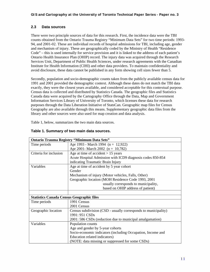
2.3 Data sources
There were two principle sources of data for this research. First, the incidence data were the TBI counts obtained from the Ontario Trauma Registry “Minimum Data Sets” for two time periods: 1993-94, and 2001-02. These are individual records of hospital admissions for TBI, including age, gender and mechanism of injury. These are geographically coded by the Ministry of Health “Residence Code” – this is used internally for service provision and it is linked to the address of each patient’s Ontario Health Insurance Plan (OHIP) record. The injury data was acquired through the Research Services Unit, Department of Public Health Sciences, under research agreements with the Canadian Institute for Health Information (CIHI) and other data providers. To maintain confidentiality and avoid disclosure, these data cannot be published in any form showing cell sizes fewer than 5. Secondly, population and socio-demographic counts taken from the publicly available census data for 1991 and 2001 provided the demographic context. Although these dates do not match the TBI data exactly, they were the closest years available, and considered acceptable for this contextual purpose. Census data is collected and distributed by Statistics Canada. The geographic files and Statistics Canada data were acquired by the Cartography Office through the Data, Map and Government Information Services Library of University of Toronto, which licenses these data for research purposes through the Data Liberation Initiative of StatsCan. Geographic map files for Census Geography are also available through this means. Supplementary geographic data files from the library and other sources were also used for map creation and data analysis. Table 1, below, summarizes the two main data sources. Table 1. Summary of two main data sources. Ontario Trauma Registry “Minimum Data Sets” Time periods Apr 1993 - March 1994 (n = 12,922)
Apr 2001- March 2002 (n = 10,782) Criteria for inclusion Age at time of accident > 15 years
Acute Hospital Admission with ICD9 diagnosis codes 850-854 indicating Traumatic Brain Injury
Variables Age at time of accident by 5 year cohort Gender Mechanism of injury (Motor vehicles, Falls, Other) Geographic location (MOH Residence Code 1993, 2001 usually corresponds to municipality, based on OHIP address of patient)
Statistics Canada Census Geographic files Time periods 1991 Census
2001 Census Geographic location Census subdivision (CSD - usually corresponds to municipality)
1991: 951 CSDs 2001: 586 CSDs (reduction due to municipal amalgamation)
Variables Population counts Age and gender by 5-year cohorts Socio-economic indicators (including Occupation, Income and Education related indicators) (NOTE: data missing or suppressed for some CSDs)
1 1

GIS and Cartography at the University of Toronto Technical Paper Series - Paper no. 3
2.4 Methodological issues raised: data and analysis
Having clarified the objectives of the study, the methodological approach, and the data sources, the methodological issues raised by this study may be classified under two categories: data issues, and analysis issues. These were encountered specifically in this study, but they can also be construed as general issues in projects of this kind. These may be summarized as follows: Data issues:
1. Geographic incompatibility (of incidence data vs. demographic data): The collected data relating to incidence may use a different geographic framework than demographic source data. Even when attempts have been made to cross-reference the two (as in our case where census geography correspondence tables for MOH Residence codes were available) differences in definition of geographic units and changes over the time period in question must be resolved.
2. Geographic accuracy: Accuracy of location provided by incidence data source may be questionable for various reasons, as specific address or postal code location is usually suppressed by data providers to maintain confidentiality of individuals.
3. Incomplete or missing demographic data: Data may contain missing or suppressed records in Census or other demographic data sources, due to problems in data collection, or due to small numbers and data collection agencies’ confidentiality restrictions.
4. Temporal incompatibility: Boundaries of geographic units used in incidence and/or demographic data collection may change over time, posing problems for comparisons between time periods.
Analysis issues:
1. Handling small values for base demographic data: Small base population numbers raise issues regarding rate calculation and representativeness of data.
2. Handling small values or zeros in incidence (TBI) data: small values or zeros in incidence values raise issues regarding rate calculation and representativeness of data. Zeros also cause problems for some spatial statistical methods, where contiguity of non-zero data units is a requirement.
3. Definition of functional “nearest neighbours” for use in spatial analysis of clusters. Spatial statistics generally use distance or contiguity between units classified as “neighbours” to build spatial weights files for identifying clusters of similar values. To be effective this classification should be based on a functional definition of “neighbours” which corresponds to the underlying model for hypothesizing spatial autocorrelation – i.e. why there would be clusters.
4. Interpretation of results of cluster and “hot spot” analysis and other spatial statistics: spatial autocorrelation statistics can identify clusters of similar data values or “hot spots”, but interpretation of these results may require on-the-ground knowledge of phenomenon and environment.
5. Incorporation of multiple variables into analysis: At present spatial regression analysis is not a mature science and the available statistical software tools are still in their early development stages.
The preparation of the data for analysis, and the treatment of these issues, is examined in detail below in sections 4.2 and 4.3.b and the attempts to resolve them are outlined.
1 2

GIS and Cartography at the University of Toronto Technical Paper Series - Paper no. 3
It is expected the outcomes resulting from this study will be the demonstration of the potential of the methodological approach, the exploration of the data and analysis issues raised, and the identification of a number of areas for future investigation.
1 3
GIS and Cartography at the University of Toronto Technical Paper Series - Paper no. 3
3. Uses of GIS and mapping to inform public health decision-making
3.1 Taking apart “Exploratory Spatial Data Analysis”
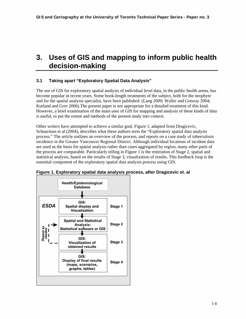
The use of GIS for exploratory spatial analysis of individual level data, in the public health arena, has become popular in recent years. Some book-length treatments of the subject, both for the neophyte and for the spatial analysis specialist, have been published. (Lang 2000; Waller and Gotway 2004; Kurland and Gorr 2006) The present paper is not appropriate for a detailed treatment of this kind. However, a brief examination of the main uses of GIS for mapping and analysis of these kinds of data is useful, to put the extent and methods of the present study into context. Other writers have attempted to achieve a similar goal. Figure 1, adapted from Dragicevic, Schuurman et al (2004), describes what these authors term the “Exploratory spatial data analysis process.” The article outlines an overview of the process, and reports on a case study of tuberculosis incidence in the Greater Vancouver Regional District. Although individual locations of incident data are used as the basis for spatial analysis rather than cases aggregated by region, many other parts of the process are comparable. Particularly telling in Figure 1 is the reiteration of Stage 2, spatial and statistical analysis, based on the results of Stage 3, visualization of results. This feedback loop is the essential component of the exploratory spatial data analysis process using GIS. Figure 1. Exploratory spatial data analysis process, after Dragicevic et. al
1 4
GIS and Cartography at the University of Toronto Technical Paper Series - Paper no. 3
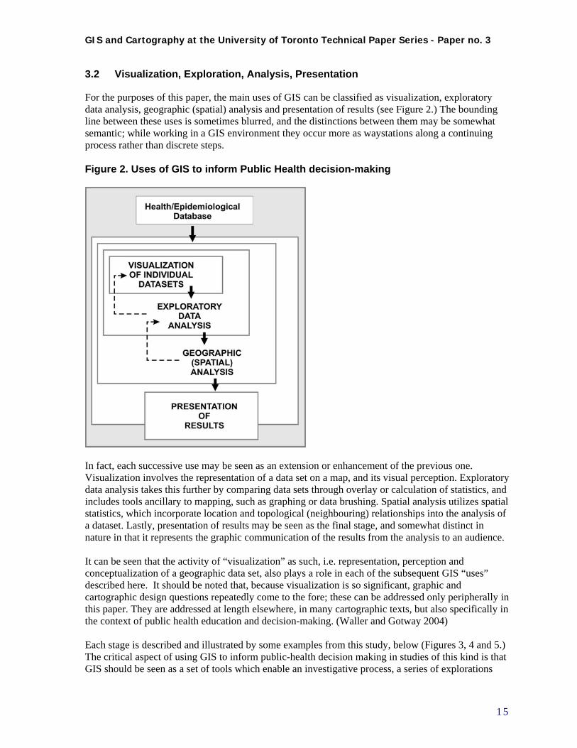
3.2 Visualization, Exploration, Analysis, Presentation
For the purposes of this paper, the main uses of GIS can be classified as visualization, exploratory data analysis, geographic (spatial) analysis and presentation of results (see Figure 2.) The bounding line between these uses is sometimes blurred, and the distinctions between them may be somewhat semantic; while working in a GIS environment they occur more as waystations along a continuing process rather than discrete steps. Figure 2. Uses of GIS to inform Public Health decision-making
In fact, each successive use may be seen as an extension or enhancement of the previous one. Visualization involves the representation of a data set on a map, and its visual perception. Exploratory data analysis takes this further by comparing data sets through overlay or calculation of statistics, and includes tools ancillary to mapping, such as graphing or data brushing. Spatial analysis utilizes spatial statistics, which incorporate location and topological (neighbouring) relationships into the analysis of a dataset. Lastly, presentation of results may be seen as the final stage, and somewhat distinct in nature in that it represents the graphic communication of the results from the analysis to an audience. It can be seen that the activity of “visualization” as such, i.e. representation, perception and conceptualization of a geographic data set, also plays a role in each of the subsequent GIS “uses” described here. It should be noted that, because visualization is so significant, graphic and cartographic design questions repeatedly come to the fore; these can be addressed only peripherally in this paper. They are addressed at length elsewhere, in many cartographic texts, but also specifically in the context of public health education and decision-making. (Waller and Gotway 2004) Each stage is described and illustrated by some examples from this study, below (Figures 3, 4 and 5.) The critical aspect of using GIS to inform public-health decision making in studies of this kind is that GIS should be seen as a set of tools which enable an investigative process, a series of explorations
1 5
GIS and Cartography at the University of Toronto Technical Paper Series - Paper no. 3
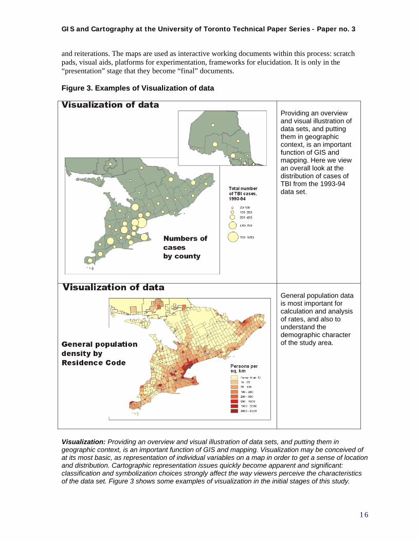
and reiterations. The maps are used as interactive working documents within this process: scratch pads, visual aids, platforms for experimentation, frameworks for elucidation. It is only in the “presentation” stage that they become “final” documents. Figure 3. Examples of Visualization of data
Providing an overview and visual illustration of data sets, and putting them in geographic context, is an important function of GIS and mapping. Here we view an overall look at the distribution of cases of TBI from the 1993-94 data set.
General population data is most important for calculation and analysis of rates, and also to understand the demographic character of the study area.
Visualization: Providing an overview and visual illustration of data sets, and putting them in geographic context, is an important function of GIS and mapping. Visualization may be conceived of at its most basic, as representation of individual variables on a map in order to get a sense of location and distribution. Cartographic representation issues quickly become apparent and significant: classification and symbolization choices strongly affect the way viewers perceive the characteristics of the data set. Figure 3 shows some examples of visualization in the initial stages of this study.
1 6
GIS and Cartography at the University of Toronto Technical Paper Series - Paper no. 3
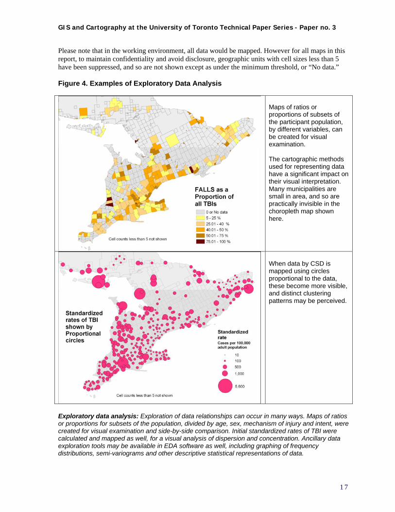
Please note that in the working environment, all data would be mapped. However for all maps in this report, to maintain confidentiality and avoid disclosure, geographic units with cell sizes less than 5 have been suppressed, and so are not shown except as under the minimum threshold, or “No data.” Figure 4. Examples of Exploratory Data Analysis
Maps of ratios or proportions of subsets of the participant population, by different variables, can be created for visual examination. The cartographic methods used for representing data have a significant impact on their visual interpretation. Many municipalities are small in area, and so are practically invisible in the choropleth map shown here.
When data by CSD is mapped using circles proportional to the data, these become more visible, and distinct clustering patterns may be perceived.
Exploratory data analysis: Exploration of data relationships can occur in many ways. Maps of ratios or proportions for subsets of the population, divided by age, sex, mechanism of injury and intent, were created for visual examination and side-by-side comparison. Initial standardized rates of TBI were calculated and mapped as well, for a visual analysis of dispersion and concentration. Ancillary data exploration tools may be available in EDA software as well, including graphing of frequency distributions, semi-variograms and other descriptive statistical representations of data.
1 7
GIS and Cartography at the University of Toronto Technical Paper Series - Paper no. 3
Figure 5. Examples of Geographic (spatial) analysis and Presentation of results
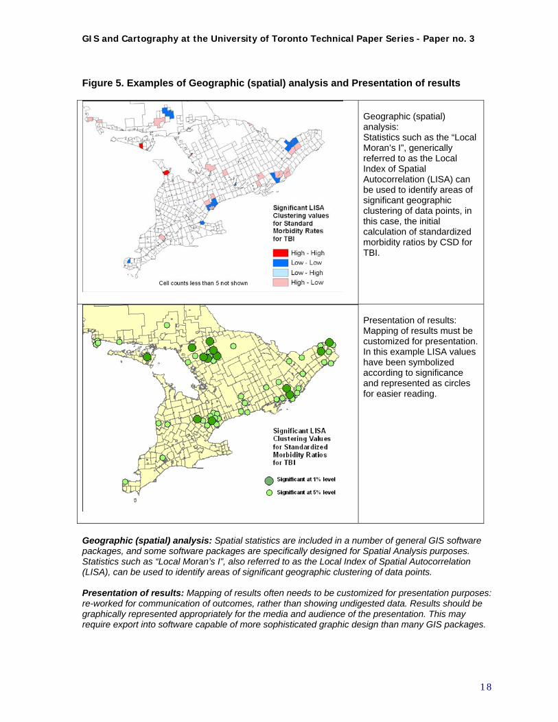
Geographic (spatial) analysis: Statistics such as the “Local Moran’s I”, generically referred to as the Local Index of Spatial Autocorrelation (LISA) can be used to identify areas of significant geographic clustering of data points, in this case, the initial calculation of standardized morbidity ratios by CSD for TBI.
Presentation of results: Mapping of results must be customized for presentation. In this example LISA values have been symbolized according to significance and represented as circles for easier reading.
Geographic (spatial) analysis: Spatial statistics are included in a number of general GIS software packages, and some software packages are specifically designed for Spatial Analysis purposes. Statistics such as “Local Moran’s I”, also referred to as the Local Index of Spatial Autocorrelation (LISA), can be used to identify areas of significant geographic clustering of data points. Presentation of results: Mapping of results often needs to be customized for presentation purposes: re-worked for communication of outcomes, rather than showing undigested data. Results should be graphically represented appropriately for the media and audience of the presentation. This may require export into software capable of more sophisticated graphic design than many GIS packages.
1 8

GIS and Cartography at the University of Toronto Technical Paper Series - Paper no. 3
4. STUDYING TBI INCIDENCE IN ONTARIO: A GIS-based APPROACH
4.1 Process undertaken and organization of report
As outlined above, this study went through two iterations of data preparation and analysis. This was in response to discoveries regarding data and analysis issues that occurred as the project proceeded. In order to put the details into context, it is useful to list the main steps in the process as they occurred, viewed in retrospect. This chronology will also be used as a framework to organize this report. 1. Review of literature on TBI and analysis of geographic disparity in public health research
2. Initial data preparation, exploration and spatial analysis
a. Data preparation before analysis to allow calculation of socio-demographic variables and standardized TBI rates by CSDs
b. Data assessment to identify data quality issues including missing data and comparability c. Initial visualization and exploratory data analysis d. Initial spatial analysis of clustering – the LISA statistic
3. Intermediate assessment and decisions regarding way forward a. GIS functionality issues – assessment and resolution b. Methodological issues (data and analysis) - assessment and attempted resolution c. Decisions on way forward
4. Second iteration: data preparation, exploration and spatial analysis a. Refinement of functional definition of nearest neighbours b. Estimation of missing data based on nearest neighbours c. Aggregation of CSDs with small populations to Minimum Population Thresholds d. Operational definition of functional nearest neighbours for analysis of clustering e. Second iteration visualization and exploratory data analysis f. Second iteration spatial analysis of clustering
5. Compilation of results a. Results – Visualization and exploratory data analysis b. Results – Spatial analysis of clustering c. Comparative analysis of 1993-94 to 2001-02
6. Conclusions and directions for future research
1 9

GIS and Cartography at the University of Toronto Technical Paper Series - Paper no. 3
4.2 Initial data preparation, exploration and spatial analysis
4.2.a Data preparation before analysis to allow calculation of socio-demographic variables and standardized TBI rates by CSDs
Data sources are outlined in section 2.3 above. Initial data preparation before analysis involves the manipulation of the TBI incidence data, census demographic data, and geographic reference files, to match TBI incidence data to census geographic areas. This provides denominators of population by age cohorts to allow the calculation of age-standardized morbidity rates by census subdistrict, and to enable linking to other socio-demographic measures provided in the census. A number of data manipulation steps must take place to achieve this linking. A graphic depiction of this initial data preparation process is illustrated in Figure 6, using the 1993-94 data injury set and the 1991 census geography as an example. The steps involved are listed below:
1. Editing of 1993-94 MOH “Residence Code to CSD conversion table” to 1991 CSDs to create correct correspondence table
2. Linking of individual TBI records 1993-94 to Census Subdivisions (CSDs) for 1991 3. Creation of CSD “count data” i.e. tables showing aggregated counts of individual TBI records
1993-94 by Census Subdivisions (CSDs) for 1991, reclassified by age cohorts (4), gender, and mechanism of injury (MV, falls, other)
4. Assembly of population data for 1991 CSDs, including a) Import of population data from census files b) Selection and construction of demographic/income variables c) Filling in missing data using estimation by closest year or closest comparable
CSD (especially for First Nations Reserves) d) Elimination of CSDs for which data are still missing
5. Calculation of age-standardized morbidity rates and ratios (SMRs) by CSD (indirect standardization using Ontario as the standard population, i.e. Ontario-wide age-specific morbidity rates to determine expected rates) (Waller and Gotway 2004 pp. 14-15).
4.2.b Data assessment to identify data quality issues including missing data and comparability
As indicated in step 4(c) above, assessment of the data during this process identified some data quality issues, especially incomplete or missing demographic data, which had to be addressed. Other data issues raised included some very small CSD totals in the population data, and many small numbers or zeros in the incidence data. These issues are common in spatial analysis of regional count data, and there are a number of methods used to address them. (Waller and Gotway 2004 pp. 201, 238) The most significant example of incomplete data in our contextual data set related to First Nations reserves, a specific type of CSD termed “Indian Reserves” [sic] in the Census data. In many cases even total population numbers were not provided for these areas, due to problems in census-taking, including political issues which resulted in non-compliance of some First Nations populations in some census years (see Appendix B) (Statistics Canada 1996; Statistics Canada 2004). It is understood that data problems regularly occur, however it became clear that omitting these territories was an undesirable solution as an apparently disproportionate number of TBI cases occurred among populations within these areas. This in turn necessitated the exploration of possible solutions to these problems, which involved more data exploration and preliminary mapping. How to estimate these populations and their characteristics? At this initial stage of analysis it was decided that an appropriate treatment would be to estimate First Nation Reserve populations based on
2 0

GIS and Cartography at the University of Toronto Technical Paper Series - Paper no. 3
the closest census years for which population data was available (eg. 1986 for 1991). Estimation of the demographic and socio-economic variables was implemented by assigning those of the three nearest comparable units, and approximating these values proportionate to population. At this initial stage, no steps were taken to deal with CSDs with very small population values. See Section 4.4 and Appendices B and C for information on how these issues were resolved. Data exploration also brought forward the challenge of temporal incompatibility of CSDs between the 1991 and 2001 censuses, primarily due to the provincial govenment’s amalgamation of many municipalities in 1998. There were 951 CSDs in Ontario in the 1991 census; these were reduced to 586 CSDs in 2001. The usual method to allow comparability in such situations would be to aggregate 1991 CSDs to match those in 2001. This was done, with some adjustment for other aggregation considerations, as outlined below in section 4.3.
2 1

GIS and Cartography at the University of Toronto Technical Paper Series - Paper no. 3
Figure 6. Initial data preparation before mapping and analysis, example of 1993-94 TBI data
2 2
GIS and Cartography at the University of Toronto Technical Paper Series - Paper no. 3
4.2.c Initial visualization and exploratory data analysis
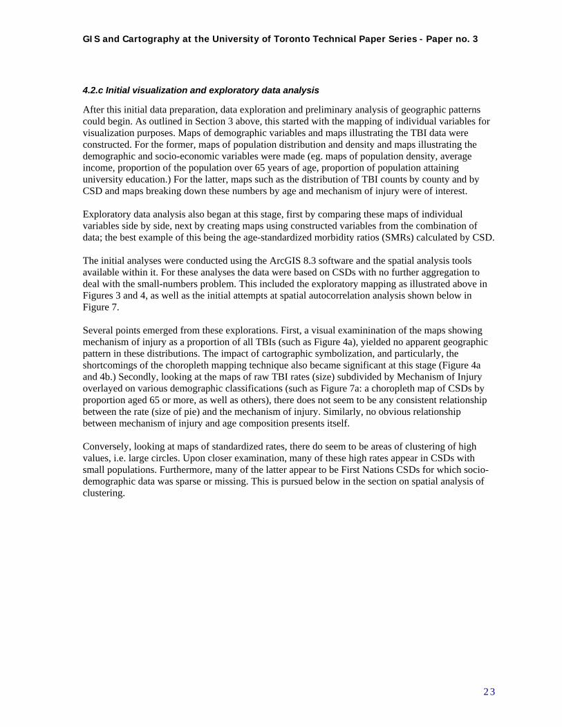
After this initial data preparation, data exploration and preliminary analysis of geographic patterns could begin. As outlined in Section 3 above, this started with the mapping of individual variables for visualization purposes. Maps of demographic variables and maps illustrating the TBI data were constructed. For the former, maps of population distribution and density and maps illustrating the demographic and socio-economic variables were made (eg. maps of population density, average income, proportion of the population over 65 years of age, proportion of population attaining university education.) For the latter, maps such as the distribution of TBI counts by county and by CSD and maps breaking down these numbers by age and mechanism of injury were of interest. Exploratory data analysis also began at this stage, first by comparing these maps of individual variables side by side, next by creating maps using constructed variables from the combination of data; the best example of this being the age-standardized morbidity ratios (SMRs) calculated by CSD. The initial analyses were conducted using the ArcGIS 8.3 software and the spatial analysis tools available within it. For these analyses the data were based on CSDs with no further aggregation to deal with the small-numbers problem. This included the exploratory mapping as illustrated above in Figures 3 and 4, as well as the initial attempts at spatial autocorrelation analysis shown below in Figure 7. Several points emerged from these explorations. First, a visual examinination of the maps showing mechanism of injury as a proportion of all TBIs (such as Figure 4a), yielded no apparent geographic pattern in these distributions. The impact of cartographic symbolization, and particularly, the shortcomings of the choropleth mapping technique also became significant at this stage (Figure 4a and 4b.) Secondly, looking at the maps of raw TBI rates (size) subdivided by Mechanism of Injury overlayed on various demographic classifications (such as Figure 7a: a choropleth map of CSDs by proportion aged 65 or more, as well as others), there does not seem to be any consistent relationship between the rate (size of pie) and the mechanism of injury. Similarly, no obvious relationship between mechanism of injury and age composition presents itself. Conversely, looking at maps of standardized rates, there do seem to be areas of clustering of high values, i.e. large circles. Upon closer examination, many of these high rates appear in CSDs with small populations. Furthermore, many of the latter appear to be First Nations CSDs for which socio-demographic data was sparse or missing. This is pursued below in the section on spatial analysis of clustering.
2 3
GIS and Cartography at the University of Toronto Technical Paper Series - Paper no. 3
Figure 7. Examples of initial data exploration and spatial analysis - using unaggregated CSD data and the ArcGIS 8.3 spatial analysis software
a) Overlay of rates and proportions: pie graphs showing raw TBI rates (size) subdivided by Mechanism of Injury overlayed on choropleth map of CSDs by proportion aged 65 or more
b) Spatial statistics such as the “Local Moran’s I” index describe the degree of clustering among data points of similar value. If the index value is positive, then that feature has values similar to neighbouring features' values. If the index value is negative, then that feature is quite different from neighbouring values.
c) Another method of determining clusters or “hotspots” in the data is the Getis-Ord Gi* statistic. Getis-Ord Gi* tests for the presence of clusters of high or low values. CSDs with absolute values greater than 1.96 indicate a significant clustering of high or low rates.
2 4

GIS and Cartography at the University of Toronto Technical Paper Series - Paper no. 3
4.2.d Initial spatial analysis of clustering – the LISA statistic
The data exploration process raised these data issues, but the case for finding a resolution for them became most compelling during the initial attempts at spatial analysis of clustering. These methods are largely based on the concept of spatial autocorrelation, which occurs when neighbouring geographic units are more similar to each other than non-neighbouring units. The main statistic utilized for this analysis is the “Local Moran’s I” statistic, also known as the Local Index of Spatial Autocorrelation, or “LISA”statistic (Anselin 1995). Spatial autocorrelation describes the relationship between the observed value of a target unit, and the values of its neighbours. Neighbours may be defined by distance or contiguity. If distance is used, a “neighbour” is considered to be any other unit within a certain distance of the target unit. Alternatively, a neighbour may be considered any unit which shares a border with the target unit (first order contiguity), or shares a border with a unit which shares a border with the target unit (second order contiguity), etc. The definition of neighbours can influence the results of any analysis. In any case, it can be seen that units which are missing data are problematic if they must be discarded from the analysis - if geographic units are “deleted”, then the defined set of any unit’s “neighbours” is affected. As mentioned, ArcGIS 8.3 was used for the initial spatial analysis. When the initial cluster analysis was run (“Cluster and Outlier Analysis – Anselin Local Moran’s I”) standard parameters were used: spatial relationship was conceptualized as Inverse Distance (the impact of one feature on another decreases with distance), with Row Standardization (Spatial weights are standardized by row, each weight being divided by its row sum). This method identified some “significant” local clustering (Figure 7b and 7c). However, the problem of small numbers and missing values cast doubt upon the results and their interpretation. Also, this software’s predisposition towards using distance-based rather than contiguity-based neighbour relationships was problematic in the context of CSDs in Ontario. Another challenge brought to the fore by the spatial analysis of clustering was the existence of multiple zero values in the TBI incidence data. The selection of acceptable analysis methodology, and therefore of software tools, was strongly influenced by this factor. Due to the use of morbidity rate data as a main variable for geographic analysis, zeros become problematic, even after standardization. An incidence of zero TBI in an area of small population will produce a rate of 0.0; an incidence of zero TBI in an area of large population will also produce a rate of 0.0. Yet clearly the latter should carry more weight than the former, as the potential opportunity for TBI is much greater. Therefore a method is required to interpolate non-zero values for rates to redress this inconsistency, and provide more useful estimates of effective morbidity rates. There are various ways of dealing with this issue, but empirical Bayes estimation has proven a useful tool for this purpose, as it smooths out the peaks and valleys of geographic data by using the values of neighbouring units to moderate very high and very low values, effectively eliminating zeros. (Waller and Gotway 2004 pp.90-95) Incorporating this methodology is difficult using some statistical software packages. Fortunately a tool was found which incorporates empirical spatial Bayes estimation into its algorithm for calculating rates for the purposes of spatial autocorrelation. (Anselin 2003b; Anselin, Lozano et al. 2006; Anselin, Syabri et al. 2006)
4.3 Intermediate assessment and decisions regarding way forward
4.3.a GIS functionality issues – assessment and resolution
The initial data exploration was therefore successful in identifying several significant challenges. In order to fulfill the objectives of the project, it became clear that the data sets as they were currently
2 5
GIS and Cartography at the University of Toronto Technical Paper Series - Paper no. 3
compiled, as well as the general-purpose GIS being used, needed re-evaluation. Regarding the data issues, these are summarized below in section 4.3.b and their resolution is discussed. Regarding GIS functionality, the areas that needed to be improved were:
1. Ability to control method of creating neighbour relationships and other parameters for spatial autocorrelation analysis
2. Ability to compare patterns of spatial autocorrelation over time 3. Ability to visualize and explore multivariate data relationships, if possible including the
ability to do spatial regression analysis
Several alternative methodological or technical solutions and combinations were investigated. The decision was made to use both ArcGIS as well as GeoDA (Anselin 2003a; Anselin 2004) a suite of software developed by Luc Anselin, in conjunction with the Center for Spatially Integrated Social Science (http://www.csiss.org/). GeoDA provides much of the functionality required for achieving the goals listed above. Where GeoDa itself falls short in terms of network analysis, and in the creation of maps for visualization and presentation, the output from GeoDa was recomposed for use in ArcGIS.
4.3.b Methodological issues (data and analysis) - assessment and attempted resolution
The generic data and analysis issues are outlined above in section 2.4 above. Tables 2 and 3 below indicate the generic issue, the specific instance encountered in this study, and the resolution of the issue, if attempted. Where necessary, further explanation of the attempted resolution is offered below. Table 2. Data issues as encountered in study Generic data issue Specific instance in this study Attempted resolution Geographic incompatibility (of incidence data vs demographic data)
Mismatch between MOH Residence codes and Census subdivision units
Detailed examination, amendment of correspondence tables between 1993-94 Residence codes and 1991 Census subdivisions, and between 2001-02 Residence codes and 2001 Census subdivisions.
Geographic accuracy Location available only at level of MOH Residence code or 3-digit postal code. Also, location based on address in OHIP record, often inaccurate due to lack of updating.
Not resolved.
Incomplete or missing demographic data
Data contains missing or suppressed CSD records in some areas in Census demographic and socio-economic data files, due to problems in data collection, or due to small numbers and StatsCan’s confidentiality restrictions.
Methods developed to estimate missing data values by using comparable data from the closest census (nearest time period) or the closest geographic units (nearest comparable neighbouring units), approximating values proportionate to population.
Temporal incompatibility
Incompatibility of Census subdivision areas between time periods (changes mainly due to amalgamation between 1991 and 2001)
Resolved by aggregation of 1991 Census subdivisions (areas and data) to match 2001 Census subdivisions to enable comparison between time periods
2 6

GIS and Cartography at the University of Toronto Technical Paper Series - Paper no. 3
The attempted resolution for “Geographic incompatibility” and “Temporal incompatibility” are self-explanatory. “Geographic accuracy” due to locational coding in the original data files was an unresolvable data constraint. “Incomplete or missing demographic data” remained a challenge. The critical missing variables were age-cohort data necessary for standardizing SMRs. Table 3. Analysis issues as encountered in study Generic analysis issue
Specific instance in this study Attempted resolution
Handling small values (very small populations) in base demographic data
Many CSDs contain small numbers in base demographic data.
Methods developed to aggregate base demographic data to Minimum Population Threshold (MPT), and to estimate missing data, based on nearest comparable neighbours.
Handling small values or zeros in incidence (TBI) data
Many zeros or small numbers in incidence (TBI) data.
Methods found which embedded interpolation algorithms (Bayes estimation) to address problems of zeros in incidence data.
Definition of functional “nearest neighbours” for use in spatial analysis of clusters
Definition of neighbouring CSDs for spatial autocorrelation analysis, when units range widely in size and organization
Neither distance nor contiguity appeared appropriate functional model, so definition based on network analysis based on transportation links between CSDs
Interpretation of results of cluster and “hot spot” analyses, and other spatial statistics
Spatial autocorrelation analysis identified a number of clusters of high standardized rates.
Possible explanations suggested but hypotheses not tested.
Incorporation of multiple variables into analysis
A number of variables were identified as possibly correlated with standardized rates, but spatial correlation was not analysed.
Not attempted.
It can be seen that the “Incomplete or missing demographic data” issue, and many of the remaining analysis issues are inter-related. It was determined that many of the solutions proposed required or would be facilitated by the determination of a consistent definition of “nearest comparable neighbour” In this context, the decisions were made:
1. to define and refine the concept of functional “nearest comparable neighbour” in the context of Ontario CSDs
2. to use this redefinition for estimating missing data values by using comparable data from the nearest comparable neighbouring CSDs
3. to use this redefinition for aggregating CSDs containing small numbers with nearest comparable neighbouring units to achieve a Minimum Population Threshold (MPT)
2 7

GIS and Cartography at the University of Toronto Technical Paper Series - Paper no. 3
4. to use this redefinition in the creation of neighbour definition and weighting matrix necessary for the calculation of spatial autocorrelation statistics, and in the interpretation of their results
“Incomplete or missing demographic data” would be estimated by using the most comparable data possible. Missing data were filled in by using comparable data from the closest census year available. Incomplete data (missing variables) were approximated by assuming the same proportions as the nearest comparable neighbouring unit.
4.3.c Decisions regarding way forward
A number of decisions were also made regarding the focus of the research effort, as it became clear that there were not sufficient resources to fully pursue all the goals of the project. The decision was made to focus on the analysis of clustering, and on the comparison of clustering patterns between the two time periods. These appeared to be the most productive avenues to follow at this stage, rather than the investigation of multivariate data relationships, given the current state of methodological tools, and the data and analysis issues involved.
4.4 Second iteration: data preparation, exploration and spatial analysis
4.4.a Refinement of definition of functional nearest neighbours
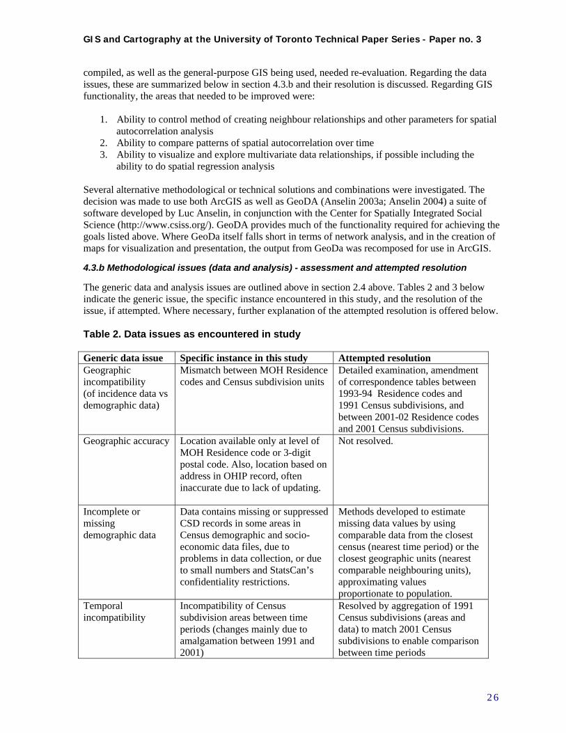
The calculation of spatial autocorrelation statistics requires the creation of a neighbour weighting matrix, which defines all the CSDs considered as neighbours for each target CSD, and the weights given to the values of those neighbouring units. In the context of CSDs in Ontario, using a simple consistent definition of “neighbour”, such as first order contiguity, was seen to cause problems. CSDs generally conform with “municipalities”. However, as can be seen from the map in Figure 8, CSDs range in type from crowded urban areas, to small towns, to compact regular townships, to isolated villages or First Nations Reserves, to huge expanses of unorganized territory. If neighbours are defined using first order contiguity, communities separated by large distances may be considered as neighbours, while ones much closer may not. If distance itself is used, the usual dimension measured is distance from the centroid (geographic centre) of one polygon to that of another. Again, CSDs may be defined as neighbours in a way which is not reflective of functional “closeness.” Therefore the decision was made to use a transportation network approach to define the “nearest neighbours” for each CSD (see Figure 9.) Essentially, a map of major highway routes (and air connections where no highway existed) was superimposed on the map of CSDs. Using the Network Analyst module in ArcGIS, a set of routes were generated for each CSD to its 10 closest neighbours, following these connections. This set of nearest neighbours was then used for three purposes: for the purposes of estimating missing values, for aggregating small CSDs to a minimum population threshold, and for creating a neighbouring weights file for spatial autocorrelation analysis. See Appendix C for a more detailed explanation of nearest neighbour analysis. In creating “nearest comparable neighbouring units” therefore, “nearest” was determined by using this network analysis approach. In determining “comparability,” however, one additional aspect was considered. It was decided that First Nations Reserves and settlements should not be considered “comparable” to other CSDs, due to the frequency of small numbers, the similar socioeconomic characteristics among many First Nations Reserves, and the fact that preliminary analysis already had identified several of these as potential clusters for TBI incidence. This meant that for First Nations CSDs, only other First Nations CSDs would be used to provide missing data, or to aggregate to a minimum population threshold, to maintain the integrity of this population as much as possible. In practice, for First Nations CSDs, the nearest alternative First Nation CSD with detailed data was utilized; for other CSDs, the nearest non-First Nation CSD was used.
2 8
GIS and Cartography at the University of Toronto Technical Paper Series - Paper no. 3
Figure 8. Census Subdivisions (CSDs) in Ontario
Figure 9. Network analysis approach to definition of CSD’s “nearest neighbours”
2 9

GIS and Cartography at the University of Toronto Technical Paper Series - Paper no. 3
4.4.b Estimation of missing data based on closest census and nearest neighbours
To estimate data for CSDs missing census data, comparable data was used from the closest census (nearest time period) or the nearest comparable neighbouring units. For CSDs missing absolute population numbers, census records from 1996 and 1986 were used to fill in population values. The nearest comparable neighbouring unit for each of these was then identified, and used as a “donor” unit. The donor’s values were applied proportionally to the total population for the unit missing data, to estimate age-sex distribution, and Occupational, Educational, and Income values for the target unit. See Appendix C for detailed explanation of estimation of missing data.
4.4.c Aggregation of CSDs with small populations to Minimum Population Thresholds
After missing data was filled in wherever possible, the next step was the aggregation of CSDs to the Minimum Population Threshold. Six rules were established for the aggregation of CSDs:
1. Populations of CSDs or aggregations of CSDs must be equal to or greater than 100 (Minimum Population Threshold)
2. Minimize the distance between CSDs forming aggregations 3. Minimize the number of CSDs forming aggregations 4. Where possible, aggregations should contain only CSDs below the MPT (i.e. avoid
aggregating CSDs that already meet the MPT) 5. Do not aggregate CSDs identified as First Nations reserves and settlements with non-First
Nations CSDs 6. Where possible, maintain comparable aggregations of CSDs between 1991 and 2001
For a more detailed explanation of the data aggregation process, see Appendix C. Table 4 summarizes the original number of CSDs in each Census year and the total number used for analysis after aggregation. After aggregation of CSDs to the MPT, the 1991 aggregations were further combined to create units for comparison between the two time periods. Note that for this inter-census comparison, the 536 CSDs for 2001 could not be used as there was not a straight many-to-one amalgamation of 1991 CSDs to create those of 2001. Further grouping of the 2001 CSDs was required to create 520 units which were comparable between the two time periods. Table 4. Summary of CSDs used for analysis
Census Year
Original no. of CSDs
CSDs missing population
No estimate available: merged into surrounding
Total aggregated CSDs used for analysis
1991 951 74 17 903
2001 586 79 (62 IRs) 27 5361991-2001 comparable 951 (1991) n/a
aggregated to make comparable to 2001 520
4.4.d Operational definition of functional nearest neighbours for analysis of clustering
The final step was the creation of the weights matrix files for the spatial autocorrelation analysis. This step is crucial, as how neighbours are defined and weighted determines whether CSDs are identified as “clustered”. At this stage a detailed visual examination of the routes generated for the CSDs took place, to identify what constituted a reasonable functional definition of neighbours, in this context.
3 0
GIS and Cartography at the University of Toronto Technical Paper Series - Paper no. 3
This had to balance the concept of travelling time along the network with the operational necessity to define at least one neighbour for each CSD. It was decided that a distance threshold of 50 km, or a half-hour highway drive, was reasonable to use as a maximum network distance between any two neighbours. Therefore, neighbours were defined as a maximum of the 10 closest comparable CSDs within a network distance of 50 km. If no neighbour was found within this distance, the closest comparable CSD at any distance along the network was defined as the single nearest neighbour. These definitions were used to construct the weights files. All neighbours were given equal weight, and row-standardized weights were used. See Appendix D for detailed explanation of weighting method.
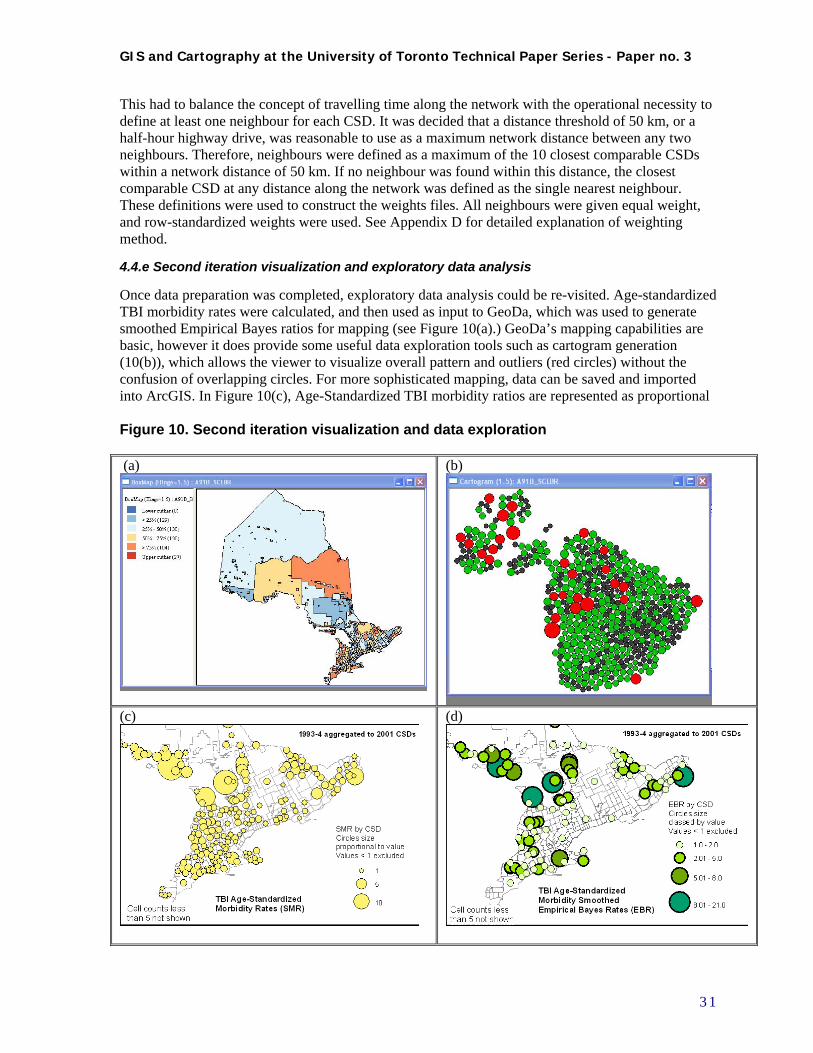
4.4.e Second iteration visualization and exploratory data analysis
Once data preparation was completed, exploratory data analysis could be re-visited. Age-standardized TBI morbidity rates were calculated, and then used as input to GeoDa, which was used to generate smoothed Empirical Bayes ratios for mapping (see Figure 10(a).) GeoDa’s mapping capabilities are basic, however it does provide some useful data exploration tools such as cartogram generation (10(b)), which allows the viewer to visualize overall pattern and outliers (red circles) without the confusion of overlapping circles. For more sophisticated mapping, data can be saved and imported into ArcGIS. In Figure 10(c), Age-Standardized TBI morbidity ratios are represented as proportional Figure 10. Second iteration visualization and data exploration (a)
(b)
(c)
(d)
3 1
GIS and Cartography at the University of Toronto Technical Paper Series - Paper no. 3
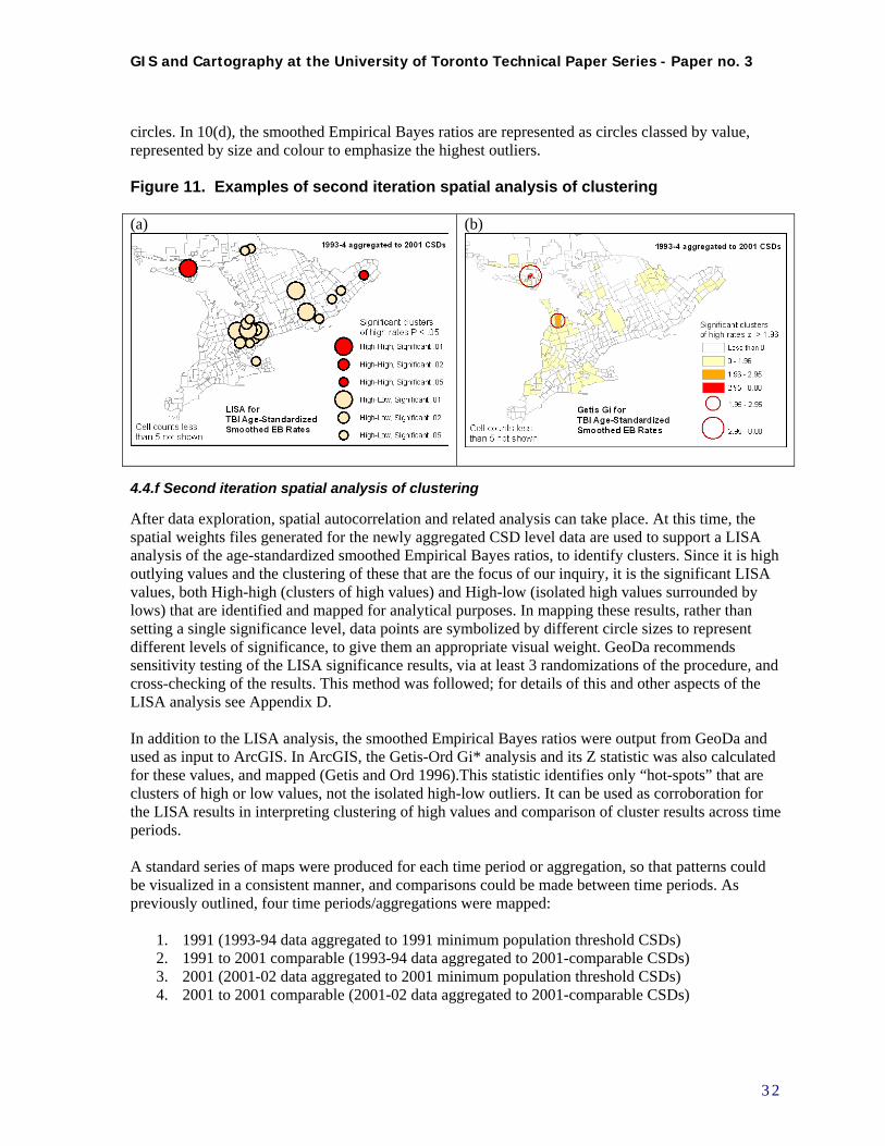
circles. In 10(d), the smoothed Empirical Bayes ratios are represented as circles classed by value, represented by size and colour to emphasize the highest outliers. Figure 11. Examples of second iteration spatial analysis of clustering (a) (b)
4.4.f Second iteration spatial analysis of clustering
After data exploration, spatial autocorrelation and related analysis can take place. At this time, the spatial weights files generated for the newly aggregated CSD level data are used to support a LISA analysis of the age-standardized smoothed Empirical Bayes ratios, to identify clusters. Since it is high outlying values and the clustering of these that are the focus of our inquiry, it is the significant LISA values, both High-high (clusters of high values) and High-low (isolated high values surrounded by lows) that are identified and mapped for analytical purposes. In mapping these results, rather than setting a single significance level, data points are symbolized by different circle sizes to represent different levels of significance, to give them an appropriate visual weight. GeoDa recommends sensitivity testing of the LISA significance results, via at least 3 randomizations of the procedure, and cross-checking of the results. This method was followed; for details of this and other aspects of the LISA analysis see Appendix D. In addition to the LISA analysis, the smoothed Empirical Bayes ratios were output from GeoDa and used as input to ArcGIS. In ArcGIS, the Getis-Ord Gi* analysis and its Z statistic was also calculated for these values, and mapped (Getis and Ord 1996).This statistic identifies only “hot-spots” that are clusters of high or low values, not the isolated high-low outliers. It can be used as corroboration for the LISA results in interpreting clustering of high values and comparison of cluster results across time periods. A standard series of maps were produced for each time period or aggregation, so that patterns could be visualized in a consistent manner, and comparisons could be made between time periods. As previously outlined, four time periods/aggregations were mapped:
1. 1991 (1993-94 data aggregated to 1991 minimum population threshold CSDs) 2. 1991 to 2001 comparable (1993-94 data aggregated to 2001-comparable CSDs) 3. 2001 (2001-02 data aggregated to 2001 minimum population threshold CSDs) 4. 2001 to 2001 comparable (2001-02 data aggregated to 2001-comparable CSDs)
3 2
GIS and Cartography at the University of Toronto Technical Paper Series - Paper no. 3
The standard series of maps consisted of the 8 listed below. All data were symbolized for TBI data at the aggregated CSD level, using a consistent symbol scaling and design for all maps in the series. For analysis purposes, all data as aggregated were mapped. For all rate data, values less than one were not mapped to reduce the visual noise introduced by the large number of non-significant values. Note that in the maps published here, to maintain confidentiality and avoid disclosure, geographic units geographic units with cell sizes less than 5 are not shown.
1. Age-standardized counts shown as proportional circles 2. Age-standardized morbidity ratios (SMRs) shown as proportional circles 3. Age-standardized morbidity ratios (SMRs) shown as classed, colour-coded circles 4. Age-standardized morbidity smoothed Empirical Bayes ratios shown as classed colour-coded
circles 5. Age-standardized morbidity ratios (SMRs) and Empirical Bayes ratios (EBRs) shown as
cartograms identifying outliers (from GeoDa – outliers identified by box plots and Box Maps where Hinge=1.5 or 3.0 – see discussion below.)
6. LISA cluster map of EBRs with colour-coded areas at consistent .05 significance level 7. LISA cluster map of EBRs shown as classed, colour-coded circles sized according to
consistent .01, .02 and .05 significance levels 8. Getis-Ord Gi* analysis map of Z statistic using choropleth method, with significantly high
values visually reinforced by classed circles sized according to .05 and .01 significant levels For an example of this standard set of maps, please see Appendix A.
4.5 Compilation of results
4.5.a Results – Visualization and exploratory data analysis
Visual analysis of data distribution as undertaken during the data exploration process is inevitably somewhat subjective, and cannot be described in an encyclopedic manner, nor should it be. It must be remembered that this is an iterative process, viewed in the context of the user’s mental map of the territory under consideration, and combined with his or her background knowledge of the conditions and phenomena under examination. The most appropriate use of GIS data exploration is for interactive comparison of different data sets, the “feedback loops” illustrated earlier in Figures 1 and 2, and development of hypotheses surrounding the issues in question. Also note that the suppression of geographic units with cell counts under 5 will change the appearance of the maps published here. Having stated these caveats, some of the patterns observed and comparisons noted may be reported. Both the 1991 and 2001 maps of age-standardized TBI counts show a strong correlation to overall population distribution, as expected. When comparing the four count maps generated for the four time periods/aggregation combinations under study, the 1991 CSDs stand out as significantly different in appearance. Counts for 1991 mapped to 1991 CSDs (n=903) look much more diffused in rural areas, much more concentrated in urban areas, than when the same counts are aggregated to 2001 comparable CSDs (n=520.) This emphasizes the fact that the “Modifiable Areal Unit Problem,” conceived of as a statistical issue, also has a corollary in the visualization context: changes in the aggregations of geographic units analysed, may make a difference in the results of the analysis. The main way of dealing with this is exclusively to use comparable maps when making comparisons. The reduction of the number of units also makes a difference during cluster analysis, as shall be seen. All the remaining maps look at age-standardized TBI ratios derived statistics, rather than counts, so that differences in population sizes are no longer an issue. In addition the ratios have been mapped excluding all values below 1. For the SMR (ratio), this represents the benchmark at which rates equal
3 3
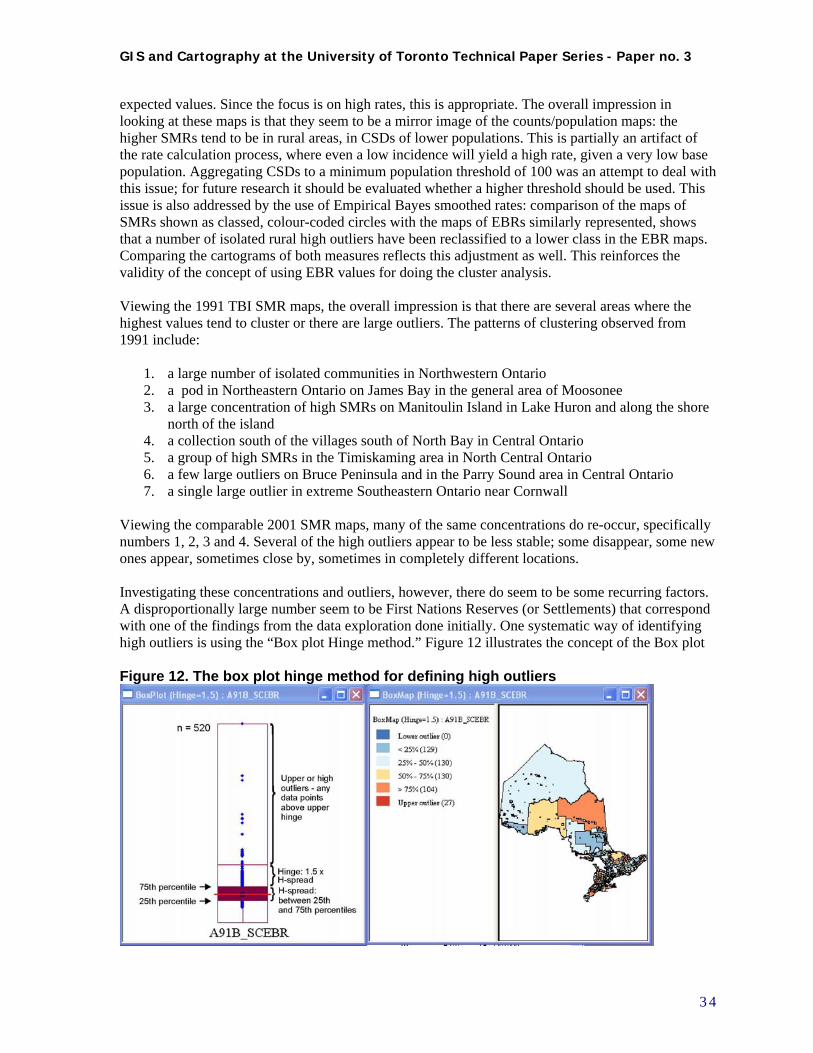
GIS and Cartography at the University of Toronto Technical Paper Series - Paper no. 3
expected values. Since the focus is on high rates, this is appropriate. The overall impression in looking at these maps is that they seem to be a mirror image of the counts/population maps: the higher SMRs tend to be in rural areas, in CSDs of lower populations. This is partially an artifact of the rate calculation process, where even a low incidence will yield a high rate, given a very low base population. Aggregating CSDs to a minimum population threshold of 100 was an attempt to deal with this issue; for future research it should be evaluated whether a higher threshold should be used. This issue is also addressed by the use of Empirical Bayes smoothed rates: comparison of the maps of SMRs shown as classed, colour-coded circles with the maps of EBRs similarly represented, shows that a number of isolated rural high outliers have been reclassified to a lower class in the EBR maps. Comparing the cartograms of both measures reflects this adjustment as well. This reinforces the validity of the concept of using EBR values for doing the cluster analysis.
Viewing the 1991 TBI SMR maps, the overall impression is that there are several areas where the highest values tend to cluster or there are large outliers. The patterns of clustering observed from 1991 include:
1. a large number of isolated communities in Northwestern Ontario 2. a pod in Northeastern Ontario on James Bay in the general area of Moosonee 3. a large concentration of high SMRs on Manitoulin Island in Lake Huron and along the shore
north of the island 4. a collection south of the villages south of North Bay in Central Ontario 5. a group of high SMRs in the Timiskaming area in North Central Ontario 6. a few large outliers on Bruce Peninsula and in the Parry Sound area in Central Ontario 7. a single large outlier in extreme Southeastern Ontario near Cornwall
Viewing the comparable 2001 SMR maps, many of the same concentrations do re-occur, specifically numbers 1, 2, 3 and 4. Several of the high outliers appear to be less stable; some disappear, some new ones appear, sometimes close by, sometimes in completely different locations. Investigating these concentrations and outliers, however, there do seem to be some recurring factors. A disproportionally large number seem to be First Nations Reserves (or Settlements) that correspond with one of the findings from the data exploration done initially. One systematic way of identifying high outliers is using the “Box plot Hinge method.” Figure 12 illustrates the concept of the Box plot Figure 12. The box plot hinge method for defining high outliers
3 4
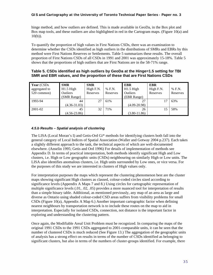
GIS and Cartography at the University of Toronto Technical Paper Series - Paper no. 3
hinge method, and how outliers are defined. This is made available in GeoDa, in the Box plot and Box map tools, and these outliers are also highlighted in red in the Cartogram maps. (Figure 10(a) and 10(b)). To quantify the proportion of high values in First Nations CSDs, there was an examination to determine whether the CSDs identified as high outliers in the distributions of SMRs and EBRs by this method were First Nations Reserves or Settlements. Table 5 summarizes these results. The overall proportion of First Nations CSDs of all CSDs in 1991 and 2001 was approximately 15-18%. Table 5 shows that the proportions of high outliers that are First Nations are in the 58-71% range.
Table 5. CSDs identified as high outliers by GeoDa at the Hinge=1.5 setting for TBI SMR and EBR values, and the proportion of these that are First Nations CSDs Year (CSDs aggregated to 520 common)
SMR H1.5 High Outliers (SMR Range)
SMR High F.N. Reserves
% F.N. Reserves
EBR H1.5 High Outliers (EBR Range)
EBR High F.N. Reserves
% F.N. Reserves
1993-94 44 (4.36-31.03)
27 61% 27 (4.09-20.98)
17 63%
2001-02 45 (4.56-23.86)
32 71% 26 (3.80-11.86)
15 58%
4.5.b Results – Spatial analysis of clustering
The LISA (Local Moran’s I) and Getis-Ord Gi* methods for identifying clusters both fall into the general category of Local Indices of Spatial Association (Waller and Gotway 2004 p.237). Each takes a slightly different approach to the task, the technical aspects of which are well-documented elsewhere. (Anselin 1995; Getis and Ord 1996) For details of implementation of methods see Appendix D. In terms of practical interpretation, both methods identify significant High and Low clusters, i.e. High or Low geographic units (CSDs) neighbouring on similarly High or Low units. The LISA also identifies anomalous clusters, i.e. High units surrounded by Low ones, or vice versa. For the purposes of this study we are interested in clusters of High values only. For interpretation purposes the maps which represent the clustering phenomenon best are the cluster maps showing significant High clusters as classed, colour-coded circles sized according to significance levels (Appendix A Maps 7 and 8.) Using circles for cartographic representation of multiple significance levels (.01, .02, .05) provides a more nuanced tool for interpretation of results than a simple binary table. Additional, as mentioned previously, any map of an area as large and diverse as Ontario using shaded colour-coded CSD areas suffers from visibility problems for small CSDs (Figure 10(a), Appendix A Map 6.) Another important cartographic factor when defining nearest neighbours by transportation network is to include these routes on the map to aid in interpretation. Especially for isolated CSDs, connection, not distance is the important factor in exploring and understanding the clustering pattern. Once again, the Modifiable Areal Unit Problem must be recognized. In comparing the maps of the original 1991 CSDs to the 1991 CSDs aggregated to 2001-comparable units, it can be seen that the number of clustered CSDs is much reduced (See Figure 13.) The aggregation of the geographic units of analysis has a strong effect on results in terms of the number of CSDs identified as belonging to significant clusters, but also in terms of the numbers of cluster-groups identified. For example, there
3 5
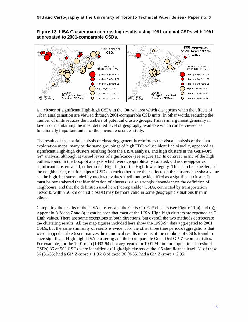
GIS and Cartography at the University of Toronto Technical Paper Series - Paper no. 3
Figure 13. LISA Cluster map contrasting results using 1991 original CSDs with 1991 aggregated to 2001-comparable CSDs.
is a cluster of significant High-high CSDs in the Ottawa area which disappears when the effects of urban amalgamation are viewed through 2001-comparable CSD units. In other words, reducing the number of units reduces the numbers of potential cluster-groups. This is an argument generally in favour of maintaining the most detailed level of geography available which can be viewed as functionally important units for the phenomena under study. The results of the spatial analysis of clustering generally reinforces the visual analysis of the data exploration maps: many of the same groupings of high EBR values identified visually, appeared as significant High-high clusters resulting from the LISA analysis, and high clusters in the Getis-Ord Gi* analysis, although at varied levels of significance (see Figure 11.) In contrast, many of the high outliers found in the Boxplot analysis which were geographically isolated, did not re-appear as significant clusters at all, either in the High-high or the High-low category. This is to be expected, as the neighbouring relationships of CSDs to each other have their effects on the cluster analysis: a value can be high, but surrounded by moderate values it will not be identified as a significant cluster. It must be remembered that identification of clusters is also strongly dependent on the definition of neighbours, and that the definition used here (“comparable” CSDs, connected by transportation network, within 50 km or first closest) may be more valid in some geographic situations than in others. Comparing the results of the LISA clusters and the Getis-Ord Gi* clusters (see Figure 11(a) and (b); Appendix A Maps 7 and 8) it can be seen that most of the LISA High-high clusters are repeated as Gi High values. There are some exceptions in both directions, but overall the two methods corroborate the clustering results. All the map figures included here show the 1993-94 data aggregated to 2001 CSDs, but the same similarity of results is evident for the other three time periods/aggregations that were mapped. Table 6 summarizes the numerical results in terms of the numbers of CSDs found to have significant High-high LISA clustering and their comparable Getis-Ord Gi* Z-score statistics. For example, for the 1991 map (1993-94 data aggregated to 1991 Minimum Population Threshold CSDs) 36 of 903 CSDs were identified as High-high clusters at the .05 significance level; 31 of these 36 (31/36) had a Gi* Z-score > 1.96; 8 of these 36 (8/36) had a Gi* Z-score > 2.95.
3 6
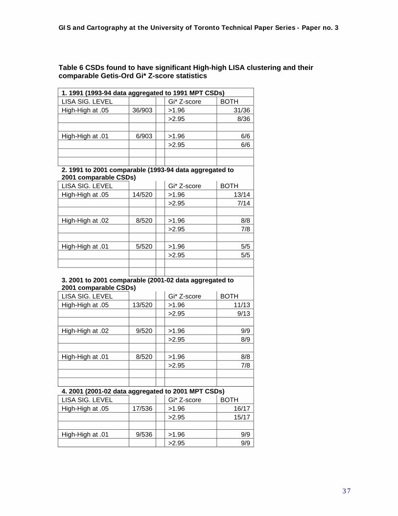
GIS and Cartography at the University of Toronto Technical Paper Series - Paper no. 3
Table 6 CSDs found to have significant High-high LISA clustering and their comparable Getis-Ord Gi* Z-score statistics 1. 1991 (1993-94 data aggregated to 1991 MPT CSDs) LISA SIG. LEVEL Gi* Z-score BOTH High-High at .05 36/903 >1.96 31/36 >2.95 8/36 High-High at .01 6/903 >1.96 6/6 >2.95 6/6 2. 1991 to 2001 comparable (1993-94 data aggregated to 2001 comparable CSDs) LISA SIG. LEVEL Gi* Z-score BOTH High-High at .05 14/520 >1.96 13/14 >2.95 7/14 High-High at .02 8/520 >1.96 8/8 >2.95 7/8 High-High at .01 5/520 >1.96 5/5 >2.95 5/5 3. 2001 to 2001 comparable (2001-02 data aggregated to 2001 comparable CSDs) LISA SIG. LEVEL Gi* Z-score BOTH High-High at .05 13/520 >1.96 11/13 >2.95 9/13 High-High at .02 9/520 >1.96 9/9 >2.95 8/9 High-High at .01 8/520 >1.96 8/8 >2.95 7/8 4. 2001 (2001-02 data aggregated to 2001 MPT CSDs) LISA SIG. LEVEL Gi* Z-score BOTH High-High at .05 17/536 >1.96 16/17 >2.95 15/17 High-High at .01 9/536 >1.96 9/9 >2.95 9/9
3 7

GIS and Cartography at the University of Toronto Technical Paper Series - Paper no. 3
Since one of the objectives of this study was the analysis of clustering, that is to find ‘hot spots’ in these patterns, it can be argued that both the LISA and Gi* methods should be used to identify potential problem areas. In the same spirit, the CSDs identified as High-low LISA clusters may also provide useful information about isolated occurrences of high rates – why would a high rate be surrounded by low neighbours? Either type of cluster may be the result of a temporary situation or – especially in CSDs with low base populations – even a unique event such as a major traffic accident. This is why the comparison of results between time periods may be helpful in identifying long-standing or chronic problem areas.
4.5.c Comparison of 1993-94 to 2001-02 data
As has been documented, a significant amount of time and resources went into the effort to make the mapping and analysis of the 1993-94 and 2001-02 TBI data compatible, including aggregating the data to common geographic units, for comparison purposes. This comparison was done using the following methods:
1. Visual comparison of patterns of the 1991, 2001 and 1991-2001 comparable series of maps (see Appendix A.)
2. Analysis of persistence of significant clustering of LISA High- values on the 1991-2001 comparable series of maps
3. Analysis of persistence of significant clustering of Getis-Ord Gi* High values on the 1991-2001 comparable series of maps
4. Comparison of persistence of significant clustering of LISA and Getis-Ord Gi* High values The visual analysis of patterns on the standard series of maps has been mentioned above, and is summarized below. The most useful comparisons are between TBI smoothed EBR significant clustering statistics (LISA and Gi*) between the two time periods, revealing persistence of clusters. Figure 14 illustrates the example of the analysis of persistence of significant LISA clustering of EBRs, contrasting results of 1993-94 with 2001-02 (shown for southern Ontario only.) Visual comparison indicates significant similarities in the patterns of high values and clustering in the earlier data series vs. the later. The most stable of these are:
1. a large number of isolated communities in Northern Ontario, East and West. 2. a large concentration of high SMRs on Manitoulin Island in Lake Huron and along the
shore north of it 3. a collection of villages south of North Bay in Central Ontario 4. a group of high SMRs in the Timiskaming area in North Central Ontario
Even among these areas, however, on close examination there is a fair amount of shifting of high rates among neighbouring CSDs, which is evidenced in the analysis of persistence of clustering, below, by the fairly small number of individual CSDs which are identified as clusters in both time periods. Even where clusters do not persist, however, comparable patterns may be repeated. A good example of this is the High-low clusters identified by the LISA analysis in Southern Ontario. These are shown as light circles in Figure 14 and Appendix A Map 7. These represent elevated rates with moderate neighbours. The cases where they don’t persist may indicate that these are the result of a temporary situation or unique event. However, the fact that there is a similar pattern of other CSDs in the same general area which have similar cluster characteristics, may indicate that there is some mechanism at work, which does have a geographic component, or that similar conditions in these Southern Ontario communities are resulting in similar kinds of TBI rate profiles, 8 years apart.
3 8
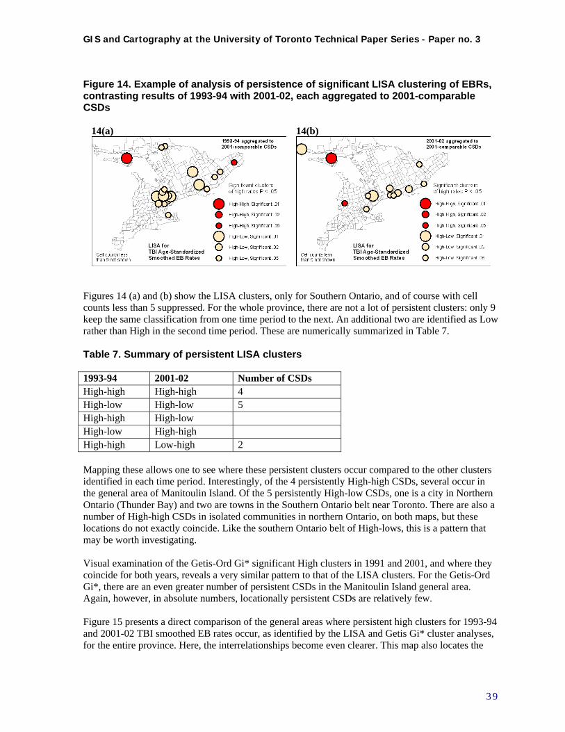
GIS and Cartography at the University of Toronto Technical Paper Series - Paper no. 3
Figure 14. Example of analysis of persistence of significant LISA clustering of EBRs, contrasting results of 1993-94 with 2001-02, each aggregated to 2001-comparable CSDs
14(a) 14(b)
Figures 14 (a) and (b) show the LISA clusters, only for Southern Ontario, and of course with cell counts less than 5 suppressed. For the whole province, there are not a lot of persistent clusters: only 9 keep the same classification from one time period to the next. An additional two are identified as Low rather than High in the second time period. These are numerically summarized in Table 7.
Table 7. Summary of persistent LISA clusters 1993-94 2001-02 Number of CSDs High-high High-high 4 High-low High-low 5 High-high High-low High-low High-high High-high Low-high 2 Mapping these allows one to see where these persistent clusters occur compared to the other clusters identified in each time period. Interestingly, of the 4 persistently High-high CSDs, several occur in the general area of Manitoulin Island. Of the 5 persistently High-low CSDs, one is a city in Northern Ontario (Thunder Bay) and two are towns in the Southern Ontario belt near Toronto. There are also a number of High-high CSDs in isolated communities in northern Ontario, on both maps, but these locations do not exactly coincide. Like the southern Ontario belt of High-lows, this is a pattern that may be worth investigating. Visual examination of the Getis-Ord Gi* significant High clusters in 1991 and 2001, and where they coincide for both years, reveals a very similar pattern to that of the LISA clusters. For the Getis-Ord Gi*, there are an even greater number of persistent CSDs in the Manitoulin Island general area. Again, however, in absolute numbers, locationally persistent CSDs are relatively few. Figure 15 presents a direct comparison of the general areas where persistent high clusters for 1993-94 and 2001-02 TBI smoothed EB rates occur, as identified by the LISA and Getis Gi* cluster analyses, for the entire province. Here, the interrelationships become even clearer. This map also locates the
3 9
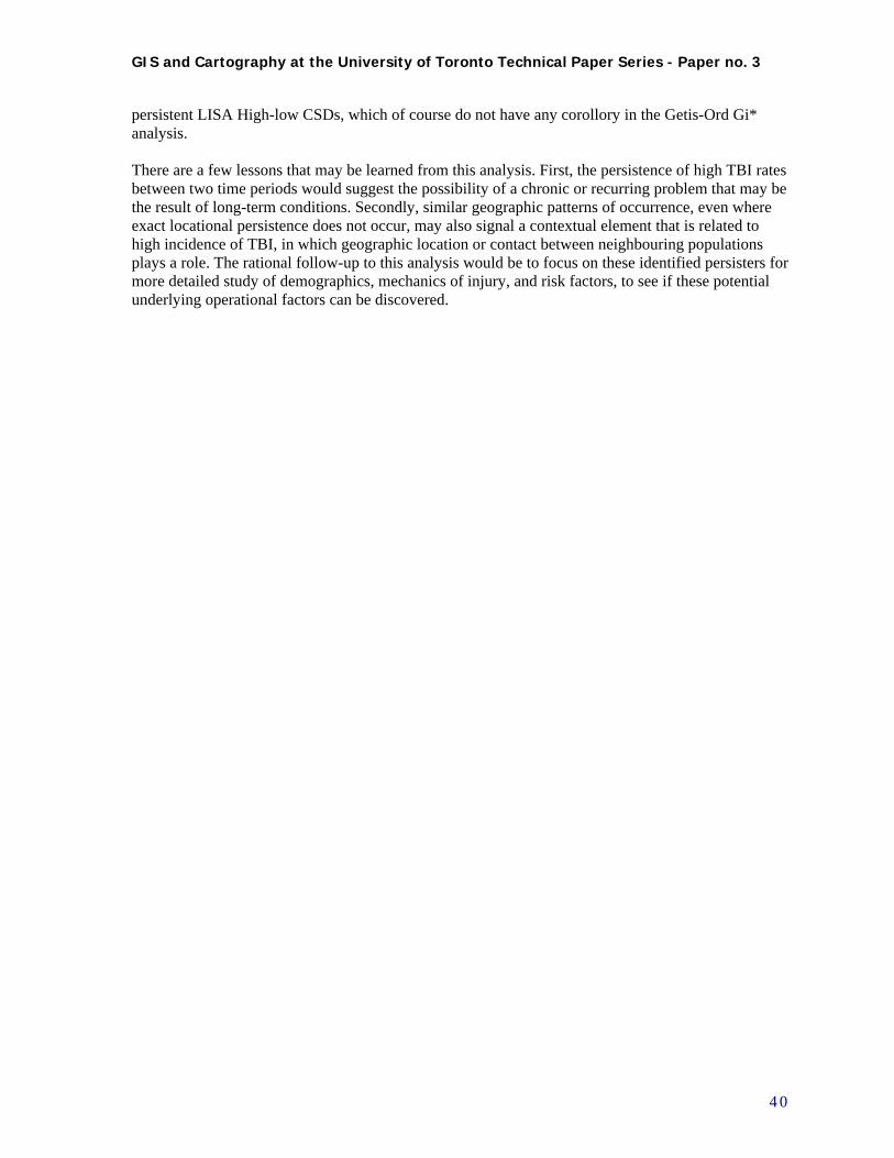
GIS and Cartography at the University of Toronto Technical Paper Series - Paper no. 3
persistent LISA High-low CSDs, which of course do not have any corollory in the Getis-Ord Gi* analysis. There are a few lessons that may be learned from this analysis. First, the persistence of high TBI rates between two time periods would suggest the possibility of a chronic or recurring problem that may be the result of long-term conditions. Secondly, similar geographic patterns of occurrence, even where exact locational persistence does not occur, may also signal a contextual element that is related to high incidence of TBI, in which geographic location or contact between neighbouring populations plays a role. The rational follow-up to this analysis would be to focus on these identified persisters for more detailed study of demographics, mechanics of injury, and risk factors, to see if these potential underlying operational factors can be discovered.
4 0
GIS and Cartography at the University of Toronto Technical Paper Series - Paper no. 3
Figure 15. Persistent high clusters for 1993-94 and 2001-02 data as identified by the LISA and Getis Gi* cluster analyses
4 1

GIS and Cartography at the University of Toronto Technical Paper Series - Paper no. 3
5. Conclusions and Directions for Future Research
The objectives of this study were to explore options and establish models for the study of TBI incidence in an interactive GIS environment related to:
1. Data exploration and preliminary analysis of geographic pattern 2. Analysis of clustering, i.e. randomness and ‘hot spots’ in these patterns 3. Analysis of change in geographic pattern over time 4. Potential for spatial regression analysis of TBI rates against socio-demographic factors.
In order to achieve these goals, much of the work in this study has dealt with the nature of the data available to pursue them, specifically in a diverse and extensive geographic area such as Ontario. The use of Regional Count data at the Census Subdivision level as the basic unit of geographic analysis for an area of this size was innovative and demanding, but necessary to deal with the issues at hand at the scale that they required. The primary methods and issues addressed have been:
1. Methods and options for visualization and analysis of epidemiological rate data in a GIS environment. Conclusion: GIS mapping and analysis tools are well advanced and adaptable to the exploration of TBI as well as other types of health-related incidence data. However, different GIS software packages have their individual strengths and weaknesses, and a combination of tools and expertise are likely necessary to address and deal properly with the variety of users’ needs.
2. Data issues regarding low incidence and base population numbers, and missing demographic data Conclusion: Appropriate use of age-standardized rates, and spatial methods for estimating missing data, data aggregation to minimum population threshold, and data smoothing, can address these issues. The experience gained in this project will be useful in improving these methods in future research.
3. Geographic issues regarding methods for aggregation of data and establishment of useful criteria for definition of neighbours in analysis of clustering Conclusion: The use of transportation network analysis methods for defining neighbours for aggregation and cluster analysis was tested during this study. These methods were found viable but further testing should be done to refine this process based on functional relationships between geographic units.
4. Use of cluster analysis as a method for identifying “hot spots” in data, and cluster persistence for comparing change in geographic pattern over time Conclusion: Two statistical methods were used for identifying “High” data clusters based on geographic neighbours: the LISA (Local Moran’s I) statistic and the Getis-Ord Gi* statistic. The results generally were consistent between the two, and appeared to identify significant clusters of high SMRs. Locational persistence rates for clusters were low between the two time periods studied. Further detailed study is necessary to evaluate the significance of these
4 2

GIS and Cartography at the University of Toronto Technical Paper Series - Paper no. 3
persistent and the non-persistent clusters, and determine whether they are indicative of important underlying factors.
The exploration of socio-demographic factors as possible explanatory variables for high TBI rates has not been systematically addressed in this study, rather a few indicators have been mentioned incidentally, and targeted for further investigation. Among others, the high incidence rates and SMRs in First Nations communities have been observed. This and other factors call out for a detailed examination which could be focused based on the results from this study. Directions for future research suggested by this study are many. It should be noted that all the data preparation work invested in this study has produced a much more comprehensive and useful data base than existed in the original raw input data, and that the potential for further use of this resource is strong, and should not be neglected. Several potential avenues for productive further research are outlined below. Regression analysis: A conventional regression analysis of the data base was attempted early in the study, to determine associations of high TBI rates with socio-demographic and economic indicators. Now that more stable estimates have been established, and a comparative geographic framework, this analysis may be re-visited. Spatial regression analysis: Software tools have been developed in GeoDa and other applications for the incorporation of neighbour relationships into regression analysis. Variables are weighted appropriately based on distance or connectivity to modify their values in determining association or dependency. These tools are still in development, but are available to do preliminary analyses which could be compared to the results of the conventional regression approach. Some very recent research has made progress in this area (Holt and Lo 2008) and may provide a model for its implementation. Bivariate LISA cluster analysis: This method for comparison to determine if two variables are related in regard to their clustering pattern could be applied to both the comparison of TBI rate data to socio-economic variables, and to the comparison of 1993-94 to 2001-02 rate data. The procedure identifies LISA clustering between two variables; the value of variable 1 at each location is compared to the values of variable 2 at all its neighbouring locations. Bivariate LISA analysis is implemented in GeoDa, but some technical problems exist in saving the resultant data and classifying its significance. These should be corrected in future releases, or work-arounds could be developed. Other Local Clustering statistics: As outlined by Waller and Gotway (2004) there are a number of other spatial statistical methods to test for geographical data clusters which may produce better results for TBI data in Ontario. Of these, the statistic they describe as “Tango’s index”, developed by Tango and refined by Rogerson (1999; 2004) may be the most promising. They describe it as “a straightforward general-purpose test of spatial clustering which incorporates aspects of tests of goodness of fit and general indexes of spatial association.” Rogerson outlines a local version of this test and also applies it to time-series data. This would be an interesting alternative method to attempt to characterize change in data clustering between time periods.
4 3
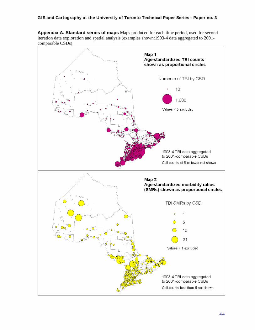
GIS and Cartography at the University of Toronto Technical Paper Series - Paper no. 3
Appendix A. Standard series of maps Maps produced for each time period, used for second iteration data exploration and spatial analysis (examples shown:1993-4 data aggregated to 2001-comparable CSDs)
4 4
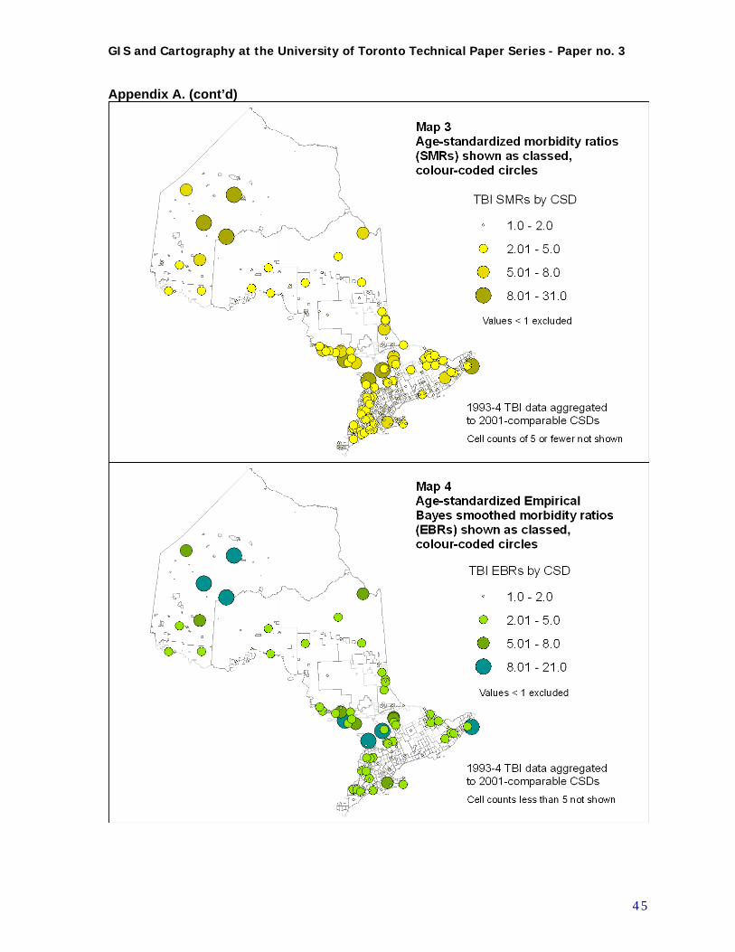
GIS and Cartography at the University of Toronto Technical Paper Series - Paper no. 3
Appendix A. (cont’d)
4 5
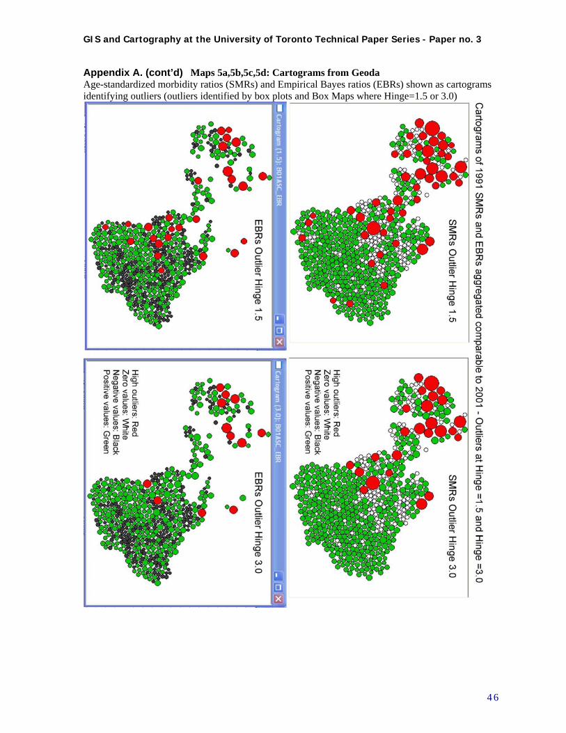
GIS and Cartography at the University of Toronto Technical Paper Series - Paper no. 3
Appendix A. (cont’d) Maps 5a,5b,5c,5d: Cartograms from Geoda Age-standardized morbidity ratios (SMRs) and Empirical Bayes ratios (EBRs) shown as cartograms identifying outliers (outliers identified by box plots and Box Maps where Hinge=1.5 or 3.0)
4 6
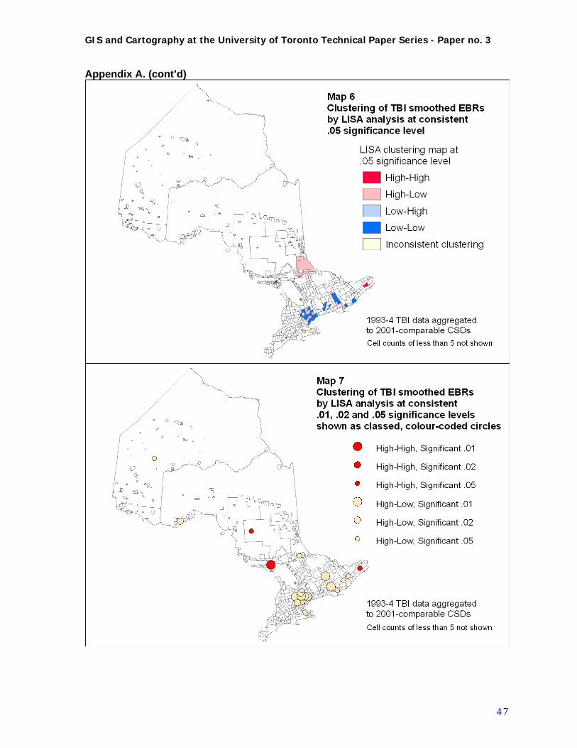
GIS and Cartography at the University of Toronto Technical Paper Series - Paper no. 3
Appendix A. (cont’d)
4 7
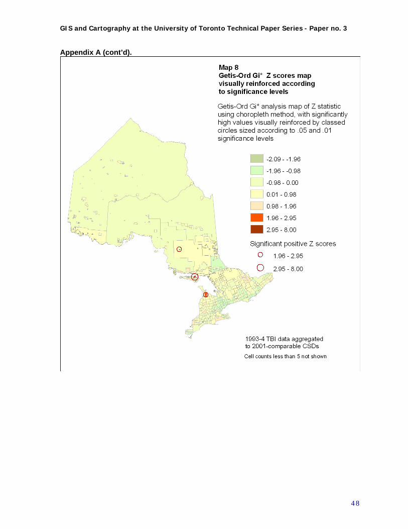
GIS and Cartography at the University of Toronto Technical Paper Series - Paper no. 3
Appendix A (cont’d).
4 8
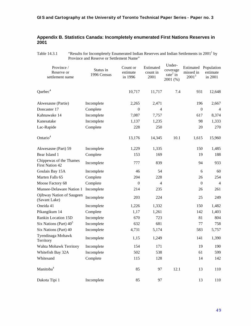
GIS and Cartography at the University of Toronto Technical Paper Series - Paper no. 3
Appendix B. Statistics Canada: Incompletely enumerated First Nations Reserves in 2001
Table 14.3.1 “Results for Incompletely Enumerated Indian Reserves and Indian Settlements in 20011 by Province and Reserve or Settlement Name”
Province / Reserve or
settlement name
Status in 1996 Census
Count or estimate in 1996
Estimated count in
2001
Under- coverage rate2 in
2001 (%)
Estimated missed in
20013
Population estimate in 2001
Quebec4 10,717 11,717 7.4 931 12,648
Akwesasne (Partie) Incomplete 2,265 2,471 196 2,667
Doncaster 17 Complete 0 4 0 4
Kahnawake 14 Incomplete 7,087 7,757 617 8,374
Kanesatake Incomplete 1,137 1,235 98 1,333
Lac-Rapide Complete 228 250 20 270
Ontario4 13,176 14,345 10.1 1,615 15,960
Akwesasne (Part) 59 Incomplete 1,229 1,335 150 1,485
Bear Island 1 Complete 153 169 19 188
Chippewas of the Thames First Nation 42
Incomplete 777 839 94 933
Goulais Bay 15A Incomplete 46 54 6 60
Marten Falls 65 Complete 204 228 26 254
Moose Factory 68 Complete 0 4 0 4
Munsee-Delaware Nation 1 Incomplete 214 235 26 261
Ojibway Nation of Saugeen (Savant Lake)
Incomplete 203 224 25 249
Oneida 41 Incomplete 1,226 1,332 150 1,482
Pikangikum 14 Complete 1,17 1,261 142 1,403
Rankin Location 15D Incomplete 670 723 81 804
Six Nations (Part) 405 Incomplete 632 681 77 758
Six Nations (Part) 40 Incomplete 4,731 5,174 583 5,757
Tyendinaga Mohawk Territory
Incomplete 1,15 1,249 141 1,390
Wahta Mohawk Territory Incomplete 154 171 19 190
Whitefish Bay 32A Incomplete 502 538 61 599
Whitesand Complete 115 128 14 142
Manitoba4 85 97 12.1 13 110
Dakota Tipi 1 Incomplete 85 97 13 110
4 9
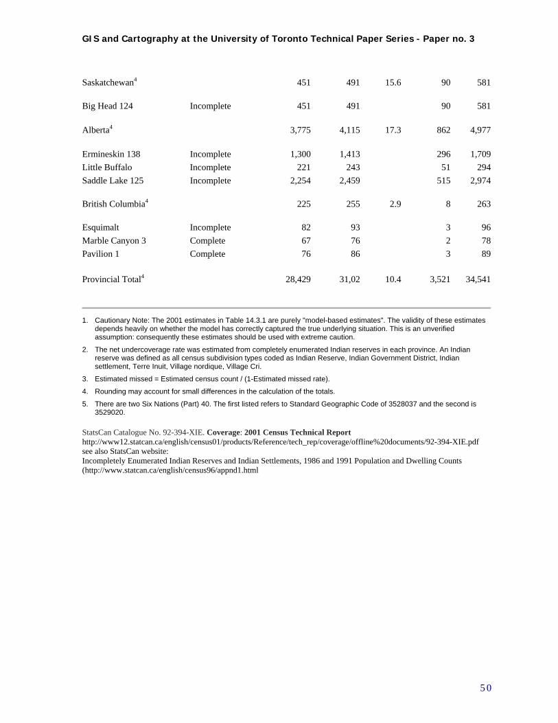
GIS and Cartography at the University of Toronto Technical Paper Series - Paper no. 3
Saskatchewan4 451 491 15.6 90 581
Big Head 124 Incomplete 451 491 90 581
Alberta4 3,775 4,115 17.3 862 4,977
Ermineskin 138 Incomplete 1,300 1,413 296 1,709
Little Buffalo Incomplete 221 243 51 294
Saddle Lake 125 Incomplete 2,254 2,459 515 2,974
British Columbia4 225 255 2.9 8 263
Esquimalt Incomplete 82 93 3 96
Marble Canyon 3 Complete 67 76 2 78
Pavilion 1 Complete 76 86 3 89
Provincial Total4 28,429 31,02 10.4 3,521 34,541
1. Cautionary Note: The 2001 estimates in Table 14.3.1 are purely "model-based estimates". The validity of these estimates depends heavily on whether the model has correctly captured the true underlying situation. This is an unverified assumption: consequently these estimates should be used with extreme caution.
2. The net undercoverage rate was estimated from completely enumerated Indian reserves in each province. An Indian reserve was defined as all census subdivision types coded as Indian Reserve, Indian Government District, Indian settlement, Terre Inuit, Village nordique, Village Cri.
3. Estimated missed = Estimated census count / (1-Estimated missed rate).
4. Rounding may account for small differences in the calculation of the totals.
5. There are two Six Nations (Part) 40. The first listed refers to Standard Geographic Code of 3528037 and the second is 3529020.
StatsCan Catalogue No. 92-394-XIE. Coverage: 2001 Census Technical Report http://www12.statcan.ca/english/census01/products/Reference/tech_rep/coverage/offline%20documents/92-394-XIE.pdf see also StatsCan website: Incompletely Enumerated Indian Reserves and Indian Settlements, 1986 and 1991 Population and Dwelling Counts (http://www.statcan.ca/english/census96/appnd1.html
5 0
GIS and Cartography at the University of Toronto Technical Paper Series - Paper no. 3
5 1
Appendix C. Second iteration data preparation: data assembly (including nearest neighbour network analysis), estimation of missing data, and aggregation to Minimum Population Threshold
C.1 Flowchart of data preparation procedures
Figure C-1 is a flowchart showing the procedures for data preparation prior to the cluster analysis which took place in the second iteration of work for this project. It is a retrospective look at this work, so incorporates the initial data preparation (see Figure 6), as well as reflecting the decisions and improvements made for the second iteration. The issues arising from small samples and missing data are addressed during this processing, decisions taken are applied, and data that are estimated and aggregated are made available for subsequent analysis. This preliminary processing has four phases: data assembly, exploratory data analysis to establish missing data and aggregation needs, estimation of missing data, and aggregation of census subdivisions to Minimum Population Thresholds. Each phase appears in order from top to bottom in the flowchart. The remainder of this section describes each of these phases and draws attention to the assumptions, decisions, and outcomes of each of them.
C.2 Data Assembly including nearest neighbour network analysis
As outlined in section 2.3 and Table 1, there are two main data sources, the TBI count data from the Ontario Trauma Registry Minimal Data Set, and the Statistics Canada Census Geographic files, and their associated Census aggregate data (population counts and demographic and socio-economic variables.) The initial data preparation using these files is outlined in the main paper in section 4.2 and illustrated in Figure 6. Initial preparation involves extracting the selected variables from the tables of census data aggregated by CSD. This is followed by joining the data to CSD subdivision boundary files in the Geographic Information System (GIS). TBI count data, identified by MOH residence codes, is aggregated by these codes. These are then converted and matched to CSDs. A significant effort was required to edit the 1993-94 MOH “Residence Code to CSD conversion table” to create correct correspondence tables to the 1991 CSDs; less effort was required for the 2001 data. The data are added to the tables of Census summary data, and together, all the data are linked to cartographic boundary files for CSDs. The main additional data assembly operation in the second round was the use of a transportation network data set (major roads augmented by air connections where needed) to build a GIS network data set, connecting nodes representing CSDs. The need for this approach is outlined in the main paper in section 4.4.a. Using the Network Analyst module in ArcGIS, a set of routes were generated for each CSD to its 10 closest neighbours, following these connections. This set of nearest neighbours is then used for three purposes: to estimate missing values, to aggregate small CSDs to a minimum population threshold, and to create a neighbouring weights file for spatial autocorrelation analysis. The steps involved in using ArcGIS Network Analyst to create the required set of functional nearest neighbours are as follows. All GIS data sets must be projected to the same projection in real-world units (metres), preferably an equidistant projection, for correct analysis.
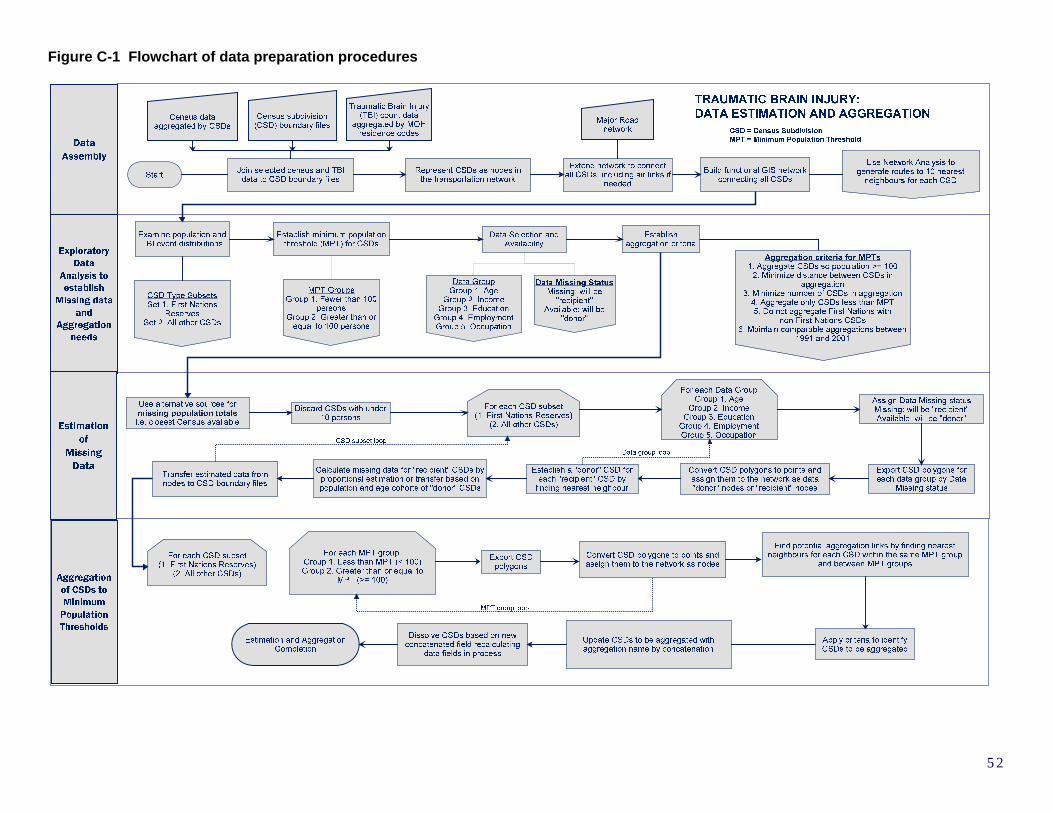
Figure C-1 Flowchart of data preparation procedures
5 2

1. Acquire linear GIS data set of major roads, and air transport routes to remote locations. (DMTI Spatial Inc. 2005) Add linear links to remote locations to road network data set.
2. Using CSD polygon data set representing CSDs, convert polygon centroids to point features. 3. Examine CSD points and transportation layer to troubleshoot connection issues. Where nec-
essary the network should be extended to reach the most remote CSDs by following patterns derived from more detailed transportation routes, including air routes.
4. Build transportation layer as an ArcGIS Network Dataset. 5. Using the Network Analyst module in ArcGIS, conduct a Closest Facility analysis. Each CSD
point is considered an “Incident”, and the object is to find the 10 closest “Facilities.” The same CSD point layer is used as the locations for both “Incidents” and “Facilities”. Detailed parameter settings required here are logical, the most critical settings and steps being:
Impedance: Length in metres Facilities to find: 11 (11 closest facilities to each incident, which includes itself) Accumulation: Length Network Locations Search Tolerance: 3 km (allowable distance between points
and linear network for establishing a connection) Load Locations of Facilities, and resolve problems of unlocated points by relo-
cating the points small distances, or extending network and rebuilding, if neces-sary
Load Locations of Incidents, since same, revised data set is being used there should be no unlocated points
Use “Solve” to effectuate the Closest Facility analysis. This will find the 10 near-est neighbours along the network for each point, and generate a set of connecting linear Routes for each solved link.
6. Export the Routes as a new GIS layer. Each route is identified in the attribute table according to its Incident ID, the connecting Facility ID, and the linear distance between them along the network.
As stated above, the set of 10 nearest neighbours was then used for three purposes: estimating missing values, aggregating small CSDs to a minimum population threshold, and for creating a neighbouring weights file for spatial autocorrelation analysis. The methods for doing this are further explained below.
C.3 Exploratory Data Analysis to establish Missing data and Aggregation needs
As described in the main paper in section 4.2.b, not all of the CSDs in Ontario have complete aggregate census data. There are 586 Census Subdivisions (CSDs) in Ontario in 2001. Exploratory data analysis established that 79 of them are missing population counts; of these 62 are classified by Statistics Canada as First Nations reserves or settlements. For 1991, there were 951 CSDs, of which 74 are missing population counts. These are summarized in Table 4. Reproduction of Table 4, Section 4.4b Summary of CSDs used for analysis
Census Year
Original no. of CSDs
CSDs missing population
No estimate available: merged into surrounding
Total aggregated CSDs used for analysis
1991 951 74 17 903
2001 586 79 (62 IRs) 27 5361991-2001 comparable 951 (1991) n/a
aggregated to make comparable to 2001 520
5 3
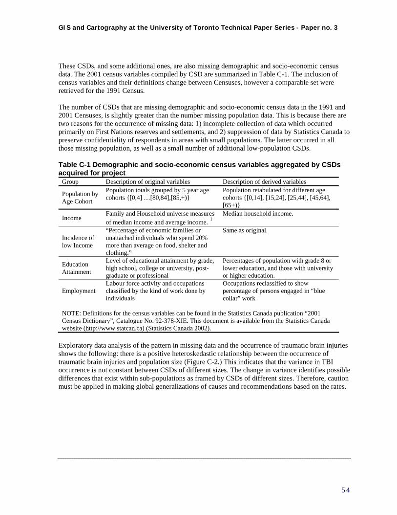
GIS and Cartography at the University of Toronto Technical Paper Series - Paper no. 3
These CSDs, and some additional ones, are also missing demographic and socio-economic census data. The 2001 census variables compiled by CSD are summarized in Table C-1. The inclusion of census variables and their definitions change between Censuses, however a comparable set were retrieved for the 1991 Census. The number of CSDs that are missing demographic and socio-economic census data in the 1991 and 2001 Censuses, is slightly greater than the number missing population data. This is because there are two reasons for the occurrence of missing data: 1) incomplete collection of data which occurred primarily on First Nations reserves and settlements, and 2) suppression of data by Statistics Canada to preserve confidentiality of respondents in areas with small populations. The latter occurred in all those missing population, as well as a small number of additional low-population CSDs. Table C-1 Demographic and socio-economic census variables aggregated by CSDs acquired for project
Group Description of original variables Description of derived variables
Population by Age Cohort
Population totals grouped by 5 year age cohorts {[0,4] …[80,84],[85,+)}
Population retabulated for different age cohorts {[0,14], [15,24], [25,44], [45,64], [65+)}
Income Family and Household universe measures of median income and average income. 1
Median household income.
Incidence of low Income
“Percentage of economic families or unattached individuals who spend 20% more than average on food, shelter and clothing.”
Same as original.
Education Attainment
Level of educational attainment by grade, high school, college or university, post-graduate or professional
Percentages of population with grade 8 or lower education, and those with university or higher education.
Employment Labour force activity and occupations classified by the kind of work done by individuals
Occupations reclassified to show percentage of persons engaged in “blue collar” work
NOTE: Definitions for the census variables can be found in the Statistics Canada publication “2001 Census Dictionary”, Catalogue No. 92-378-XIE. This document is available from the Statistics Canada website (http://www.statcan.ca) (Statistics Canada 2002).
Exploratory data analysis of the pattern in missing data and the occurrence of traumatic brain injuries shows the following: there is a positive heteroskedastic relationship between the occurrence of traumatic brain injuries and population size (Figure C-2.) This indicates that the variance in TBI occurrence is not constant between CSDs of different sizes. The change in variance identifies possible differences that exist within sub-populations as framed by CSDs of different sizes. Therefore, caution must be applied in making global generalizations of causes and recommendations based on the rates.
5 4
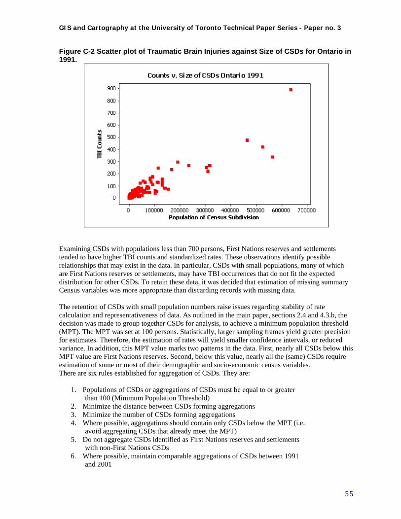
GIS and Cartography at the University of Toronto Technical Paper Series - Paper no. 3
Figure C-2 Scatter plot of Traumatic Brain Injuries against Size of CSDs for Ontario in 1991.
Examining CSDs with populations less than 700 persons, First Nations reserves and settlements tended to have higher TBI counts and standardized rates. These observations identify possible relationships that may exist in the data. In particular, CSDs with small populations, many of which are First Nations reserves or settlements, may have TBI occurrences that do not fit the expected distribution for other CSDs. To retain these data, it was decided that estimation of missing summary Census variables was more appropriate than discarding records with missing data. The retention of CSDs with small population numbers raise issues regarding stability of rate calculation and representativeness of data. As outlined in the main paper, sections 2.4 and 4.3.b, the decision was made to group together CSDs for analysis, to achieve a minimum population threshold (MPT). The MPT was set at 100 persons. Statistically, larger sampling frames yield greater precision for estimates. Therefore, the estimation of rates will yield smaller confidence intervals, or reduced variance. In addition, this MPT value marks two patterns in the data. First, nearly all CSDs below this MPT value are First Nations reserves. Second, below this value, nearly all the (same) CSDs require estimation of some or most of their demographic and socio-economic census variables. There are six rules established for aggregation of CSDs. They are:
1. Populations of CSDs or aggregations of CSDs must be equal to or greater than 100 (Minimum Population Threshold)
2. Minimize the distance between CSDs forming aggregations 3. Minimize the number of CSDs forming aggregations 4. Where possible, aggregations should contain only CSDs below the MPT (i.e.
avoid aggregating CSDs that already meet the MPT) 5. Do not aggregate CSDs identified as First Nations reserves and settlements
with non-First Nations CSDs 6. Where possible, maintain comparable aggregations of CSDs between 1991
and 2001
5 5

GIS and Cartography at the University of Toronto Technical Paper Series - Paper no. 3
The first rule has just been addressed. The next two rules (2, 3) keep aggregations as small and compact as possible, presumably minimizing the differences within aggregations. The fourth rule assumes it preferable to avoid aggregating CSDs that meet the MPT. This is because aggregation can reduce the interpretability of results, so where possible, areas that meet the MPT should remain intact. The fifth rule is based on initial observations that small CSDs, many of which are First Nations reserves, have TBI rates that may not fit the expected distribution. Retaining their identifying characteristic may reveal patterns later in the analysis. Finally, rule 6 makes it possible to conduct intercensal comparisons.
C.4 Estimation of Missing Data
To estimate data for CSDs missing population counts, the best available comparable data was used from the closest prior census years available (1996, 1991 or 1986) or other Statistics Canada sources. These sources include Statistics Canada’s Table 14.3.1 “Results for incompletely enumerated Indian Reserves and Settlements” [sic] (see Appendix B.) There were 27 CSDs for 2001 and 17 for 1991 for which population counts or good estimates could not be obtained. These CSDs were discarded by merging them with their surrounding areas. Missing demographic and socio-economic data for CSDs is estimated by using the most comparable data possible, based on a nearest neighbour analysis, and CSD type. First CSDs are assigned a Data Missing Status. CSDs missing data are identified as “recipients”; CSDs containing data are identified as potential “donors.” Then CSDs are separated into two groups by type: First Nations Reserves, and all other CSDs. Estimation of missing data is based on a nearest neighbour approach using the linear distances calculated for CSDs along the GIS network (see Figure 9). Only one nearest neighbour is used as the source of estimated data. The premise of using the nearest neighbour approach is the assumption that places closer together are more alike than places farther apart. Using more than one source can reduce estimation error, however this is most valid when all points contain data and all points are evenly spaced. In the case of CSDs, in particular with First Nations reserves and settlements, finding more than one neighbour for any single estimation may involve looking in different directions over quite different distances. All CSDs are not missing the same census data. Thus, for each group of variables as listed in Table C-1, CSDs are identified as either “recipients” or potential “donors”. Then, for each of these groups, for each recipient, the nearest neighbouring “donor” of the comparable type is found. Count data is estimated for recipients using proportions based on population and age cohorts of donors. Variables expressed as percentages or median values are transferred directly from the donor to the recipient CSD.
C.5 Aggregation of CSDs to Minimum Population Thresholds
Aggregation of CSDs, which do not meet the MPT, is completed in a manner similar to the estimation of missing data. All CSDs are divided into two groups, those that meet the MPT and those that do not. For each of the CSDs below the MPT, potential aggregation links are identified by finding nearest neighbours within the same MPT group and between MPT groups; i.e. a first set of nearest neighbours chosen only from those CSDs below the MPT, a second set of nearest neighbours are chosen from those CSDs which already meet the MPT. These two sets are derived to adhere to rule five for aggregation.
5 6

GIS and Cartography at the University of Toronto Technical Paper Series - Paper no. 3
Potential aggregations of nearest neighbours are then evaluated using the aggregation rules for MPTs, and the best aggregations selected. Aggregations are identified by concatenating the names of the CSDs forming the group. After selecting the groups for aggregation, they are “dissolved” in the GIS, which produces multi-part CSDs that may be non-contiguous. These multi-part CSDs share a common name, and data is recalculated. Count data for aggregated CSDs are summed while medians are averaged. Since medians of constituent CSDs may vary, the lowest and highest values are retained in the dissolved aggregation to indicate the range of the constituent data. See Appendix D for details of methods of weighting nearest neighbours and conducting spatial autocorrelation analyses.
5 7

GIS and Cartography at the University of Toronto Technical Paper Series - Paper no. 3
Appendix D Second iteration data analysis: Creation of neighbouring weights file and spatial autocorrelation analysis
D.1 Method for weighting of nearest neighbours prior to spatial autocorrelation analysis
Section 4.4.a above, gives the justification for the refinement of the definition of functional nearest neighbours in the context of CSDs in Ontario, for the purpose of spatial autocorrelation analysis (also termed “cluster” analysis.) Section 4.4.d outlines the operational definition of functional nearest neighbours, for the purpose of creating the matrix files for the spatial autocorrelation analysis. After the network analysis identifying 10 nearest neighbours for each CSD was completed, a detailed visual examination of the routes generated for the CSDs took place. For the purpose of the weights matrix, the definition of neighbours had to balance the concept of travelling time along the network with the operational necessity to define at least one neighbour for each CSD. It was decided that generally, neighbours were to be defined as a maximum of the 10 closest comparable CSDs within a network distance of 50 km. If no neighbour was found within this distance, the closest comparable CSD at any distance along the network was defined as the single nearest neighbour, with some exceptions. The exceptions to these criteria were the 10 very large, mostly rural CSDs in northern Ontario, described as “unorganized” CSDs by Statistics Canada. These are extensive areas with little population, scattered around in isolated settlements. The location of the point-feature centroid in such cases, and the distance between centroids, is meaningless in terms of our concept of a definition of functional nearest neighbours. It was decided to treat these exceptions as a different type of CSD, comparable to themselves. These were isolated in a separate GIS layer, and neighbours defined by First order “Queen” contiguity. When no neighbours were identified by this process, a neighbour was assigned by visual examination and manual operation. These definitions were used to construct the weights files. All neighbours were given equal weight, and row-standardized weights were used. Weights matrix files must identify neighbours and weights, however file formats vary in specifications according to the different software used to generate and use them. Since these files were to be used in the GeoDA software, they were created using that specification. GeoDA allows two formats for weights files: Contiguity weights (.GAL) and Distance weights (.GWT), the latter were used for this analysis. (Anselin 2003b) These may be created automatically in GeoDA from the polygon shape file to be analysed, and this was done for the initial round of analysis. Since for the second iteration of analysis a refined definition was used, the files were artificially constructed.
D.2 Artificial construction of neighbouring weights: Distance weights file
The format of the Distance weights files is represented in Figure D-1, by an excerpt from the weights file from the 1991-2001 comparable CSD file. The first line describes the file parameters, the follow-ing lines go in order from polygon 1 through 520, with each line representing one neighbour relation-ship. Although distances between polygons are recorded in the file, neighbouring weights were not calculated proportionally to distances for the spatial autocorrelation analysis; row-standardized weights were used, in which for each CSD, all CSDs identified as neighbours were given equal weight in calculating the spatial lag variable (i.e. Weight = 1 divided by number of neighbours.)
5 8
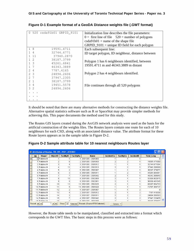
GIS and Cartography at the University of Toronto Technical Paper Series - Paper no. 3
Figure D-1 Example format of a GeoDA Distance weights file (.GWT format) 0 520 csda91b01 GRPID_9101 Initialization line describes the file parameters:
0 = first line of file 520 = number of polygons csda91b01 = name of the shape file GRPID_9101 = unique ID field for each polygon
1 8 19591.4711 1 4 32744.6771 1 11 37940.2870 1 2 38187.3799 1 3 45261.6841 1 7 46343.3889 2 4 7787.4165 2 3 24894.2606 2 7 37947.2305 2 1 38187.3799 3 4 19451.5578 3 2 24894.2606 . . . . . . . . .
Each subsequent line: ID target polygon, ID neighbour, distance between Polygon 1 has 6 neighbours identified, between 19591.4711 m and 46343.3889 m distant Polygon 2 has 4 neighbours identified. File continues through all 520 polygons
It should be noted that there are many alternative methods for constructing the distance weights file. Alternative spatial statistics software such as R or SpaceStat may provide simpler methods for achieving this. This paper documents the method used for this study. The Routes GIS layers created during the ArcGIS network analysis were used as the basis for the artificial construction of the weights files. The Routes layers contain one route for each of 10 neighbours for each CSD, along with an associated distance value. The attribute format for these Route layers appears as in the sample table in Figure D-2. Figure D-2 Sample attribute table for 10 nearest neighbours Routes layer
However, the Route table needs to be manipulated, classified and extracted into a format which corresponds to the GWT files. The basic steps in this process were as follows:
5 9

GIS and Cartography at the University of Toronto Technical Paper Series - Paper no. 3
1. Add 5 new fields for data linking, classification and extraction process, including last 3 for WEIGHTS format as per .GWT file: ORIG_NAME, NEAR_NAME (text fields, for name of origin CSD and nearest neighbour) ORIG_GRPID, NEAR_GRPID (integer, for unique ID of origin CSD and nearest neighbour) DISTANCE (floating, for DISTANCE) 2. Use VBScripts to extract strings from “Name” field, which has the name of the Origin and Destination CSD, and assign these to ORIG_NAME and NEAR_NAME fields 3. To populate the ORIG_GRPID field: Make sure grouped CSD layer has a unique identifier field GRPID_YEAR. Temporarily join Routes layer attribute table to grouped CSD table (from item ORIG_NAME to corresponding NAME field in grouped CSD table); then: Calculate ORIG_GRPID = GRPID_YEAR 4. To populate the NEAR_GRPID field: Temporarily join Routes layer attribute table to grouped CSD table (from item NEAR_NAME to corresponding NAME field in grouped CSD table); then: Calculate NEAR_GRPID = GRPID_YEAR 5. To classify Route records to fit our Nearest neighbour criteria, for export into WEIGHTS file: Select by attributes to get all routes less than 50 km and greater than 0. For selected routes, Calculate: DISTANCE = “Total_Leng” Then: Select by attributes to get all routes where there is no neighbour closer than 50 km. Reselect from current selection: "FacilityRa" = 2 AND "Total_Leng" > 50000 (Facility Rank should be 2, not 1, as First rank for every facility is itself) Reselect from current selection: For selected routes, Calculate: DISTANCE = “Total_Leng” The results of these calculations is represented in Figure D-3. Figure D-3 Sample attribute table for Routes layer with new fields added and calculated
6. To export as weights file, preliminary format: Select by attributes where: DISTANCE > 0; with these selected, Use Options->Export data table and save as: Dbase file (TBI_NN_YEAR_WTS.dbf)
6 0
GIS and Cartography at the University of Toronto Technical Paper Series - Paper no. 3
This file can then be manipulated in Dbase or Excel to simulate the GWT weights file format. Delete all columns except last 3. Sort data on ORIG_GRPID, and DISTANCE and check to confirm all consecutive IDs exist in file from 1 to maximum. Reformat DISTANCE column to required number of decimal places. Insert an empty column before the DISTANCE column. 7. For Unorganized CSDs to be treated as exceptions, isolate these in a separate GIS shape file, and use GeoDA to generate a weights file defined by First order “Queen” contiguity (.GAL file.) When no neighbours were identified by this process, a neighbour was assigned by visual examination and manual operation. Incorporate these “artificial” nearest neighbours into the simulated .GWT file with an artificially supplied distance of 99999.99 m to flag them. 8. Finally, export the simulated GWT file as a .CSV text file, replace the initial line which holds field names with the GWT format initialization line, and use a text editor to replace commas with appropriate blank spaces, and save with a .GWT extension. This final .GWT file can then be used in GeoDA to conduct the spatial autocorrelation LISA analysis.
D.3 Methods for spatial autocorrelation analysis – LISA and Getis-Ord Gi*
Sections 4.4.e and 4.4.f. of the main paper deal with the second iteration of visualization and exploratory data analysis, and the spatial analysis of clustering. Figures 10 and 11, and Appendix A, represent the mapping and analysis done for these purposes. The main spatial autocorrelation analysis undertaken was the LISA analysis using GeoDA; a corroborative analysis using the Getis-Ord Gi* was done in ArcGIS, using the rates output from GeoDA. This section gives a more detailed explanation of the calculations and methods involved to conduct these analyses. All calculations of rates were based on the age-standardized count variable. For each time period, the TBI age-standardized morbidity ratio (SMR) for each CSD (or aggregated CSDs) was calculated by the indirect standardization method outlined in Waller and Gotway(2004). This rate was then applied to the total TBI count variable for each CSD to arrive at an adjusted standardized count value (SCOUNT.) These calculations were all done in Excel. This was then used in GeoDA for all further rate calculations and mapping. Creation of the SMRs and SCOUNT variable was necessary because age-standardization cannot be done within GeoDA. Once these fields were generated and integrated into the CSD shape files, these were brought into GeoDA. Initially, GeoDA was used to do exploratory data analysis and visualization by means of Box plots, Box maps, and Cartograms, on these variables. Then, the SCOUNT variable was used in GeoDA to calculate smoothed Empirical Bayes ratios, map them, and conduct LISA analysis using them as input. The steps for this process are outlined below.
1. Open GeoDA project and select correct shape file for CSD aggregation and year; and Key va-riable which appears as unique ID in shape file and in corresponding .GWT weights file.
2. Use Box plots, Box maps and Cartograms to do data visualization. For Cartograms, the fol-lowing settings were generally used: Options -> Improve cartogram with: 500 iterations Options -> Change the HINGE value to 3.0 from default 1.5 These graphics and maps are only created as temporary onscreen displays, and therefore must be saved as image files for future visual comparison or import into reports.
6 1

GIS and Cartography at the University of Toronto Technical Paper Series - Paper no. 3
3. Create LISA with EB map for each time period, using the Space->LISA with EB Rate tool. These should be for the age-standardized Count variable, SCOUNT, as rates and EB smooth-ing is calculated automatically. For RATE SMOOTHING dialog: Event variable: SCOUNT variable Base variable (denominator for rate calculation): Total population age 15 or more Select Weight: appropriate .GWT weights file Windows to open: all 4 (Cluster map, Significance map, Box plot, Scatterplot) Use Options -> Randomization -> 999 in order to apply 999 permutations. Use Options -> Significance Filter -> .05 to set a level for significant spatial correlation cate-gory Use Options-> Save results ... to save calculated values: for the LISA statistic (LI), Spatial Correlation category (CL), and Significance probability value (PV). (“The LISA Local Moran statistics for each location, the association p-value and the classifi-cation of significant (at p < 0.05) locations by type of spatial correlation can be saved to the data table by means of the Options > Save Results command. For both the Local Moran and the significance level the actual values are stored. For the spatial correlation type an indicator value is stored, which takes on the value of 1 for high-high, 2 for low-low, 3 for low-high and 4 for high-low.”) (Anselin 2003a)
4. GeoDa recommends sensitivity testing of the LISA significance results, via at least 3 ran-
domizations of the procedure, and cross-checking of the results. As a sensitivity analysis, multiple randomizations should be run and their results captured, then compared. When these are run, the LISA index value will remain constant (therefore does not have to be re-saved) but the Significance probability value (PV) and therefore the Spatial Correlation category (CL) will vary. To achieve the multiple randomizations, do two more randomizations, with the same settings as in point 3, saving these resultant calculated values each time to new fields flagged as the results from Randomizations 2 and 3 Use Options->Save to Shape file as: ... to save calculated values to shape file, or else they will NOT be retained in shape file data. The Significance probability value (PV) and Spatial Correlation category (CL) values from randomizations 1, 2 and 3 can then be cross-checked against each other. For the LISA cluster analysis only CSDs identified as significant clusters at the .05 level in all three randomiza-tions were assumed to be “consistent” significant clusters, for mapping purposes (eg. Appen-dix A, Map 6: LISA cluster map of EBRs with colour-coded areas at consistent .05 signifi-cance level.)
5. In order to use calculated smoothed Empirical Bayes rates as input to ArcGIS for mapping and analysis purposes, these were also calculated and added and saved as separate fields for all CSD shape files using method: Space-> Moran’s I with EB Rate
To corroborate the results of the LISA cluster analysis in GeoDa, an attempt was made to do a similar analysis in ArcMap, using the “Hot Spot analysis” Getis-Ord Gi* statistic, found under Spatial Statistics -> Mapping Clusters. This method is capable of using a Weights file similar to the GeoDa .GWT file for input. (Minor editing of the GWT weights file is necessary - the top line contains only the ID field.) See Figure D-4 showing tool graphic user interface for settings used in this analysis.
6 2
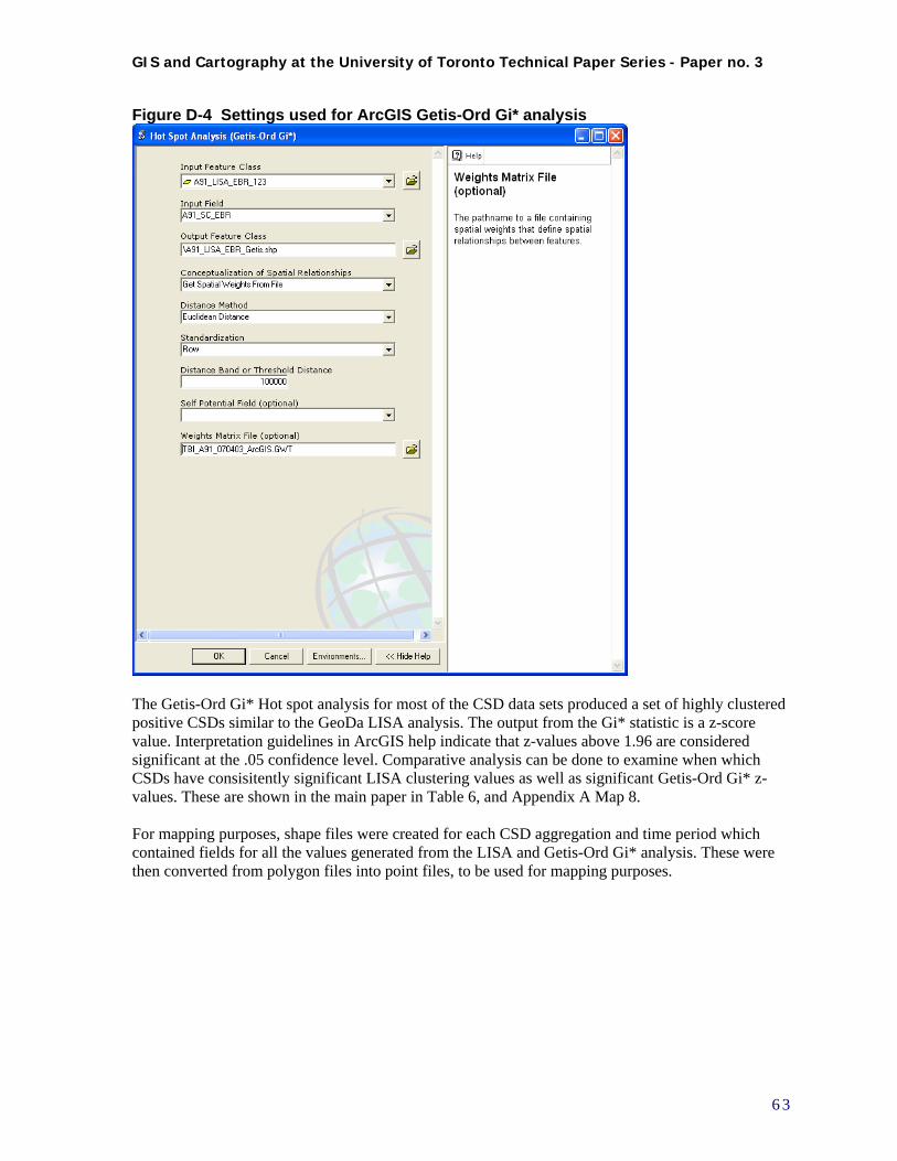
GIS and Cartography at the University of Toronto Technical Paper Series - Paper no. 3
Figure D-4 Settings used for ArcGIS Getis-Ord Gi* analysis
The Getis-Ord Gi* Hot spot analysis for most of the CSD data sets produced a set of highly clustered positive CSDs similar to the GeoDa LISA analysis. The output from the Gi* statistic is a z-score value. Interpretation guidelines in ArcGIS help indicate that z-values above 1.96 are considered significant at the .05 confidence level. Comparative analysis can be done to examine when which CSDs have consisitently significant LISA clustering values as well as significant Getis-Ord Gi* z-values. These are shown in the main paper in Table 6, and Appendix A Map 8. For mapping purposes, shape files were created for each CSD aggregation and time period which contained fields for all the values generated from the LISA and Getis-Ord Gi* analysis. These were then converted from polygon files into point files, to be used for mapping purposes.
6 3

GIS and Cartography at the University of Toronto Technical Paper Series - Paper no. 3
Bibliography
Altmayer, C. A., B. G. Hutchison, et al. (2003). "Geographic Disparity in Premature Mortality in
Ontario." International Journal of Health Geographics 2(7).
Anselin, L. (1995). "Local Indicators of Spatial Association - LISA." Geographical Analysis 27: 93-115.
Anselin, L. (2003a). "GeoDa 0.9 User's Guide."
Anselin, L. (2003b). "GeoDa - An Introduction to Spatial Data Analysis."
Anselin, L. (2004). "GeoDa 0.9.5-i Release Notes." from https://www.geoda.uiuc.edu/.
Anselin, L., N. Lozano, et al. (2006). "Rate Transformations and Smoothing." from http://sal.uiuc.edu/.
Anselin, L., I. Syabri, et al. (2006). "GeoDa: An Introduction to Spatial Data Analysis." Geographical Analysis 38(1): 5-23.
Aultman-Hall, L. and M. G. Kaltenecker (1999). "Toronto Bicycle Commuter Safety Rates." Accident Analysis and Prevention 31: 675-686.
Baker, S. P., A. Waller, et al. (1991). "Motor vehicle Deaths in Children: Geographic Variations." Accident Analysis and Prevention 23: 19-28.
Braddock, M., G. Lapidus, et al. (1994). "Using a Geographic Information System to Understand Child Pedestrian Injury." American Journal of Public Health 84(7): 1158-1161.
Colantonio, A., R. Croxford, et al. (2008, in press). "Trends in hospitalization associated with traumatic brain injury in Ontario, 1992-2001." Journal of Trauma & Critical Care.
Cromley, K. E. (2003). "GIS and disease." Annual Review of Public Health 24: 7-24.
Cusimano, M. D., M. Chipman, et al. (2007). "Geomatics in Injury Prevention: The Science, the Potential and the Limitations." Injury Prevention 13(1): 51-56.
Department of Pesticide Regulation (2005). The Department of Pesticide Regulation DPR Databases, Department of Pesticide Regulation, Sacramento CA.
DMTI Spatial Inc. (2005). CanMap Route Logistics Ontario v2005.3, DMTI Spatial Inc.
6 4

GIS and Cartography at the University of Toronto Technical Paper Series - Paper no. 3
Dragicevic, S., N. Schuurman, et al. (2004). "The Utility of Exploratory Spatial Data Analysis in the Study of Tuberculosis Incidences in an Urban Canadian Population." Cartographica 39: 29-39.
Ecosystem Science and Technology Branch. (2004). "Center for Health Applications of Aerospace Related Technologies (CHAART)." 2004, from http://geo.arc.nasa.gov/sge/health/chaart.html.
European Health and Environment Information (2005). European Health and Environment Information System for Disease and Exposure Mapping and Risk Assessment EUROHEIS,. Copenhagen, European Health and Environment Information.
Gabella, B., R. E. Hoffman, et al. (1997). "Urban and Rural Traumatic Brain Injuries in Colorado." Annals of Epidemiology 7(3): 207-212.
Getis, A. and J. K. Ord (1996). Local Spatial Statistics: An Overview. Spatial Analysis: Modelling in a GIS Environment. P. Longley and M. Batty. Cambridge, Geoinformation International.
Hijar, M. and M. Bronfman (2003). "Pedestrian Injuries in Mexico: A Multi-method approach." Social Science and Medicine 57: 2149-2159.
Holt, J. B. and C. P. Lo (2008). "The geography of mortality in the Atlanta metropolitan area " Computers, Environment and Urban Systems 32(2): 149-164.
Jarup, L. (2004). "Health and Environment Information Systems for Exposure and Disease Mapping, and Risk Assessment." Environmental Health Perspectives 112: 995-997.
Kistemann, T., F. Dangendorf, et al. (2002). "New Perspectives on the Use of Geographic Information Systems (GIS) in Environmental Health Sciences." International Journal of Hygiene and Environment Health 205: 169-181.
Kraus, J. F., M. A. Black, et al. (1984). "The Incidence of Acute Brain Injury and Serious Impairment in a Defined Population." American Journal of Epidemiology 119(2): 186-201.
Kurland, K. S. and W. L. Gorr (2006). GIS tutorial for health. Redlands, Calif., ESRI Press.
Lang, L. (2000). GIS for Health Organizations. Redlands, California, United States, ESRI Press.
Lascala, E. A., D. Gerber, et al. (2000). "Demographic and Environmental correlates of Pedestrian Injury Collisions: A Spatial Analysis." Accident Analysis and Prevention 32: 651-658.
Mallonee, S., G. R. Istre, et al. (1996). "Surveillance and Prevention of Residential-Fire Injuries." New England Journal of Medicine 335: 27-31.
McLafferty, S. L. (2003). "GIS and Healthcare." Annual Review of Public Health 24: 7-24.
National Cancer Institute. (2005). "Cancer Mortality Maps & Graphs." from http://www3.cancer.gov/atlasplus/.
National Center for Injury Prevention and Control. (2005). "Injury Maps." Retrieved 2005, from www.cdc.gov/ncipc/maps.
6 5

GIS and Cartography at the University of Toronto Technical Paper Series - Paper no. 3
6 6
Nuckols, J. R., M. H. Ward, et al. (2004). "Using Geographic Information Systems for Exposure Assessment in Environmental Epidemiology Studies." Environmental Health Perspectives 112: 1007-1015.
Pickett, W., R. Das-Gupta, et al. (2002). "Traumatic Brain Injury." Disability Rehabilitation 24: 654-665.
Robinson, T. P. (2000). "Spatial Statistics and Geographical Information Systems in Epidemiology and Public Health." Adv Parasitol 47: 81-128.
Rogerson, P. A. (1999). "The Detection of Clusters Using A Spatial Version of the Chi-Square Goodness of Fit Statistic." Geographical Analysis 31(1): 130-147.
Rogerson, P. A. (2004). The Application of New Spatial Statistical Methods to the Detection of Geographical Patterns of Crime. Applied GIS and Spatial Analysis. J. Stillwell and G. Clarke. Hoboken, New Jersey, United States, John Wiley and Sons.
Statistics Canada. (1996). "Incompletely Enumerated Indian Reserves and Indian Settlements, 1986 and 1991 Population and Dwelling Counts." Statistics Canada, 2008, from http://www.statcan.ca/english/census96/appnd1.html.
Statistics Canada (2002). 2001 Census Dictionary (Reference Products: 2001 Census) Catalogue No. 92-378-XIE. Ottawa, Statistics Canada.
Statistics Canada (2004). Coverage, 2001 Census Technical Report (Reference Products 2001 Census) Catalogue No. 92-394-XIE. Chapter 14. Refusal Indian Reserves and Settlements. Ottawa, Statistics Canada.
Waller, L. A. and C. A. Gotway (2004). Applied Spatial Statistics for Public Health Data. Atlanta, Georgia, United States, John Wiley & Sons.
Wang, S. and P. J. Smith (1997). "In Quest of 'Forgiving' Environment: Residential planning and Pedestrian Safety in Edmonton, Canada." Planning Perspectives 12: 225-250.
Williams, K. G., M. Schootman, et al. (2003). "Geographic Variation of Pediatric Burn Injuries in a Metropolitan Area." Academic Emergency Medicine 10: 743-752.
Woodward, A., M. M. Dorsch, et al. (1984). "Head Injuries in Country and City. A Study of Hospital Separations in South Australia." Medical Journal of Australia 141: 13-17.
Yiannakoulias, N., B. H. Rowe, et al. (2003). "Zones of Prevention: The Geography of Fall Injuries in the Elderly." Social Science and Medicine 57: 2065-2073.