Embed Size (px)
Citation preview
NUMERICAL METHODS FOR SOLVING THE CAHN-HILLIARD EQUATION AND ITSAPPLICABILITY TO MIXTURES OF NEMATIC-ISOTROPIC FLOWS WITH ANCHORING
EFFECTS
Giordano Tierra Chica
Department of MathematicsTemple University
In collaboration with:Francisco Guillén González
María Ángeles Rodríguez BellidoUniversidad de Sevilla, Seville, Spain
Special Thanks to : Christian Zillinger
May 2016 Giordano Tierra Approximating energy-based models
1/68
1 Motivation
2 Second order schemes and time-step adaptivity for theCahn-Hilliard equation
Cahn-Hilliard ModelSecond Order SchemesApproximations of potential term f k (φn+1, φn)Time step adaptivityNumerical Simulations
3 Linear unconditional energy-stable splitting schemes fornematic-isotropic flows with anchoring effects
Nematic Liquid CrystalsMixtures of Nematic Liquid Crystals with Newtonian fluidThe modelNumerical schemesNumerical simulations
4 References
May 2016 Giordano Tierra Approximating energy-based models
1/68

Phase field or Diffuse interface models
• Sharp-interface models• PDE for each phase + coupled interface conditions• Very difficult numerically (interface tracking)
• Diffuse interface Phase-field models• Phase function with distinct values (for instance +1 and -1) in
each phase, with a smooth change in the interface (of widthε).
• Surface motion depending on the physical energydissipation.
• When interface width ε tends to zero, recover a sharpinterface model.
May 2016 Giordano Tierra Approximating energy-based models
2/68
Motivation
Design numerical schemes for diffuse-interface phase-fieldproblems:
1 Efficient in time (Linear schemes, adaptive time-step).2 Suitable to use (standard) Finite Elements (mesh
adaptation)3 Mimic properties of the continuous problem: Dissipative
Energy law, maximum principle, mass conservation, ...4 Good finite and large time accuracy (infinite equilibrium
states)
Numerical analysis:1 Large time Energy Stability2 Unique Solvability of the schemes3 Convergence of iterative algorithms approximating nonlinear
schemes
May 2016 Giordano Tierra Approximating energy-based models
3/68
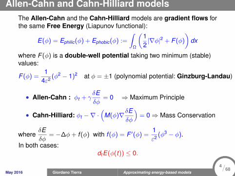
Allen-Cahn and Cahn-Hilliard modelsThe Allen-Cahn and the Cahn-Hilliard models are gradient flows forthe same Free Energy (Liapunov functional):
E(φ) = Ephilic(φ) + Ephobic(φ) :=
∫Ω
(12|∇φ|2 + F (φ)
)dx
where F (φ) is a double-well potential taking two minimum (stable)values:
F (φ) =1
4ε2 (φ2 − 1)2 at φ = ±1 (polynomial potential: Ginzburg-Landau)
• Allen-Cahn : φt + γδEδφ
= 0 ⇒ Maximum Principle
• Cahn-Hilliard: φt −∇ ·(
M(φ)∇δEδφ
)= 0⇒ Mass Conservation
whereδEδφ
= −∆φ+ f (φ) with f (φ) = F ′(φ) =1ε2 (φ3 − φ).
In both cases:dtE(φ(t)) ≤ 0.
May 2016 Giordano Tierra Approximating energy-based models
4/68
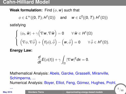
Cahn-Hilliard Model
Weak formulation: Find (φ,w) such that
φ ∈ L∞((0,T ); H1(Ω)) and w ∈ L2((0,T ); H1(Ω))
satisfying〈φt , w〉+ γ
(∇w ,∇w
)= 0 ∀ w ∈ H1(Ω)(
∇φ,∇φ)
+(
f (φ), φ)−(
w , φ)
= 0 ∀ φ ∈ H1(Ω).
Energy Law:
ddt
E(φ(t)) + γ
∫Ω|∇w |2dx = 0.
Mathematical Analysis: Abels, Garcke, Grasselli, Miranville,Schimperna, ...Numerical Analysis: Boyer, Elliot, Feng, Gómez, Hughes, Prohl,...
May 2016 Giordano Tierra Approximating energy-based models
5/68

Second Order Schemes for the Cahn-Hilliard model
Generic Second order Finite Difference schemes (Crank-Nicolsonfor linear terms)(δtφ
n+1, w)
+ γ(∇wn+ 1
2 ,∇w)
= 0 ∀ w ∈ H1(Ω)(∇(φn+1 + φn
2
),∇φ
)+(
f k (φn+1, φn), φ)−(
wn+ 12 , φ)
= 0 ∀ φ ∈ H1(Ω),
where δtφn+1 = (φn+1 − φn)/k (discrete time derivative).
Discrete Energy Law: Testing by (w , φ) = (wn+ 12 , δtφ
n+1)
δtE(φn+1) + γ‖∇wn+ 12 ‖2
L2 +((((((((hhhhhhhhNDphilic(φn+1, φn) + NDphobic(φn+1, φn) = 0,
where
NDphilic(φn+1, φn) :=(∇(φn+1 + φn
2
),∇δtφ
n+1)−δt
(∫Ω
12|∇φn+1|2
)= 0
and
NDphobic(φn+1, φn) :=(
f k (φn+1, φn), δtφn+1)− δt
(∫Ω
F (φn+1)
)May 2016 Giordano Tierra Approximating energy-based models
6/68
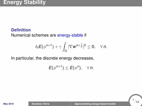
Energy Stability
DefinitionNumerical schemes are energy-stable if
δtE(φn+1) + γ
∫Ω|∇wn+ 1
2 |2 ≤ 0, ∀n.
In particular, the discrete energy decreases,
E(φn+1) ≤ E(φn), ∀n.
May 2016 Giordano Tierra Approximating energy-based models
7/68
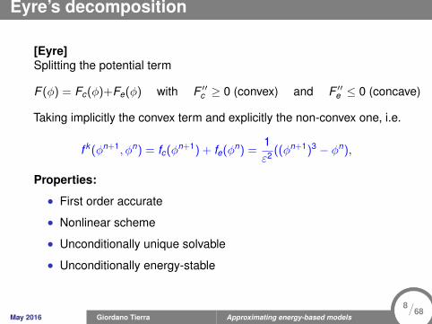
Eyre’s decomposition
[Eyre]Splitting the potential term
F (φ) = Fc(φ)+Fe(φ) with F ′′c ≥ 0 (convex) and F ′′e ≤ 0 (concave)
Taking implicitly the convex term and explicitly the non-convex one, i.e.
f k (φn+1, φn) = fc(φn+1) + fe(φn) =1ε2 ((φn+1)3 − φn),
Properties:
• First order accurate
• Nonlinear scheme
• Unconditionally unique solvable
• Unconditionally energy-stable
May 2016 Giordano Tierra Approximating energy-based models
8/68
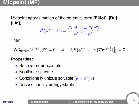
Midpoint (MP)
Midpoint approximation of the potential term [Elliot], [Du],[Lin],...
f k (φn+1, φn) =F (φn+1)− F (φn)
φn+1 − φn
Then
NDphobic(φn+1, φn) = 0 ⇒ δtE(φn+1) + γ‖∇wn+ 12 ‖2L2 = 0
Properties:• Second order accurate• Nonlinear scheme• Conditionally unique solvable (k < ε4/γ)
• Unconditionally energy-stable
May 2016 Giordano Tierra Approximating energy-based models
9/68
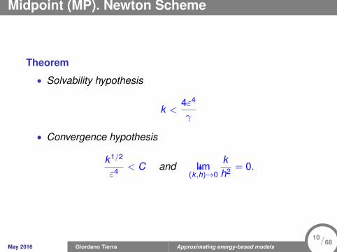
Midpoint (MP). Newton Scheme
Theorem
• Solvability hypothesis
k <4ε4
γ
• Convergence hypothesis
k1/2
ε4 < C and l«ım(k ,h)→0
kh2 = 0.
May 2016 Giordano Tierra Approximating energy-based models
10/68
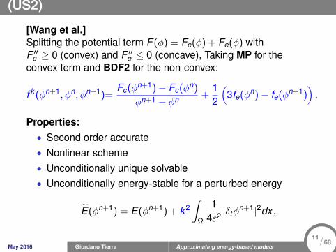
(US2)
[Wang et al.]Splitting the potential term F (φ) = Fc(φ) + Fe(φ) withF ′′c ≥ 0 (convex) and F ′′e ≤ 0 (concave), Taking MP for theconvex term and BDF2 for the non-convex:
f k (φn+1, φn, φn−1)=Fc(φn+1)− Fc(φn)
φn+1 − φn +12
(3fe(φn)− fe(φn−1)
).
Properties:• Second order accurate• Nonlinear scheme• Unconditionally unique solvable• Unconditionally energy-stable for a perturbed energy
E(φn+1) = E(φn+1) + k2∫
Ω
14ε2 |δtφ
n+1|2dx ,
May 2016 Giordano Tierra Approximating energy-based models
11/68
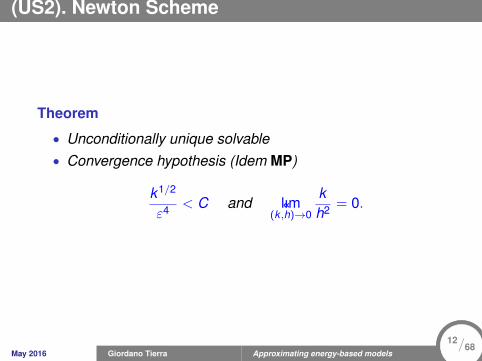
(US2). Newton Scheme
Theorem
• Unconditionally unique solvable• Convergence hypothesis (Idem MP)
k1/2
ε4 < C and l«ım(k ,h)→0
kh2 = 0.
May 2016 Giordano Tierra Approximating energy-based models
12/68
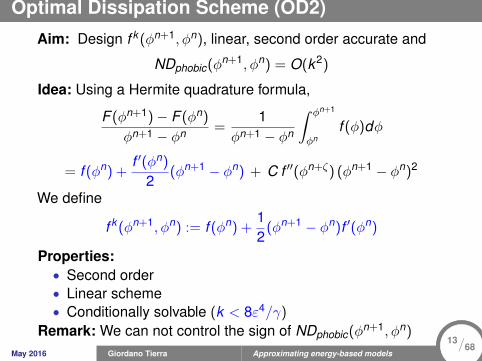
Optimal Dissipation Scheme (OD2)
Aim: Design f k (φn+1, φn), linear, second order accurate and
NDphobic(φn+1, φn) = O(k2)
Idea: Using a Hermite quadrature formula,
F (φn+1)− F (φn)
φn+1 − φn =1
φn+1 − φn
∫ φn+1
φnf (φ)dφ
= f (φn) +f ′(φn)
2(φn+1 − φn) + C f ′′(φn+ζ) (φn+1 − φn)2
We define
f k (φn+1, φn) := f (φn) +12
(φn+1 − φn)f ′(φn)
Properties:• Second order• Linear scheme• Conditionally solvable (k < 8ε4/γ)
Remark: We can not control the sign of NDphobic(φn+1, φn)
May 2016 Giordano Tierra Approximating energy-based models
13/68
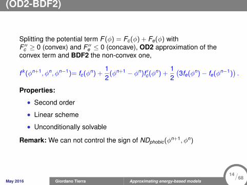
(OD2-BDF2)
Splitting the potential term F (φ) = Fc(φ) + Fe(φ) withF ′′c ≥ 0 (convex) and F ′′e ≤ 0 (concave), OD2 approximation of theconvex term and BDF2 the non-convex one,
f k (φn+1, φn, φn−1)= fc(φn) +12
(φn+1 − φn)f ′c(φn) +12(3fe(φn)− fe(φn−1)
).
Properties:
• Second order
• Linear scheme
• Unconditionally solvable
Remark: We can not control the sign of NDphobic(φn+1, φn)
May 2016 Giordano Tierra Approximating energy-based models
14/68
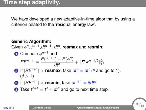
Time step adaptivity.
We have developed a new adaptive-in-time algorithm by using acriterion related to the ’residual energy law’.
Generic Algorithm:Given φn, φn−1,dtn−1, dtn, resmax and resmin:
1 Compute φn+1 and
REn+1 :=E(φn+1)− E(φn)
dtn + ‖∇wn+1/2‖2L2 .
2 If |REn+1| > resmax, take dtn = dtn/θ and go to 1).(θ > 1)
3 If |REn+1| < resmin, take dtn+1 = θdtn.4 Take tn+1 = tn + dtn and go to next time step.
May 2016 Giordano Tierra Approximating energy-based models
15/68
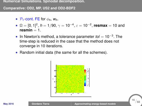
Numerical Simulations. Spinodal decomposition.
Comparative: OD2, MP, US2 and OD2-BDF2
• P1-cont. FE for φh, wh.
• Ω = [0,1]2, h = 1/90, γ = 10−4, ε = 10−2, resmax = 10 andresmin = 1.
• In Newton’s method, a tolerance parameter tol = 10−3. Thetime-step is reduced in the case that the method does notconverge in 10 iterations.
• Random initial data (the same for all the schemes).
May 2016 Giordano Tierra Approximating energy-based models
16/68
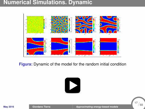
Numerical Simulations. Dynamic
Figura: Dynamic of the model for the random initial condition
May 2016 Giordano Tierra Approximating energy-based models
17/68
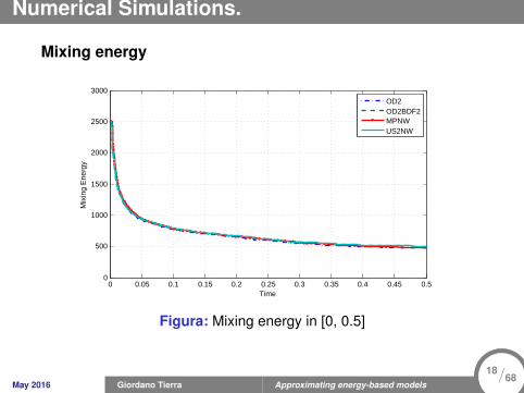
Numerical Simulations.
Mixing energy
0 0.05 0.1 0.15 0.2 0.25 0.3 0.35 0.4 0.45 0.50
500
1000
1500
2000
2500
3000
Time
Mix
ing
Ene
rgy
OD2OD2BDF2MPNWUS2NW
Figura: Mixing energy in [0, 0.5]
May 2016 Giordano Tierra Approximating energy-based models
18/68
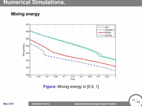
Numerical Simulations.
Mixing energy
0.5 0.55 0.6 0.65 0.7 0.75 0.8 0.85 0.9 0.95 1380
400
420
440
460
480
500
520
Time
Mix
ing
Ene
rgy
OD2OD2BDF2MPNWUS2NW
Figura: Mixing energy in [0.5, 1]
May 2016 Giordano Tierra Approximating energy-based models
19/68
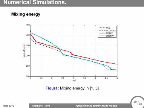
Numerical Simulations.
Mixing energy
1 1.5 2 2.5 3 3.5 4 4.5 5200
250
300
350
400
450
Time
Mix
ing
Ene
rgy
OD2OD2BDF2MPNWUS2NW
Figura: Mixing energy in [1, 5]
May 2016 Giordano Tierra Approximating energy-based models
20/68
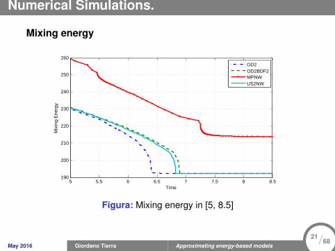
Numerical Simulations.
Mixing energy
5 5.5 6 6.5 7 7.5 8 8.5190
200
210
220
230
240
250
260
Time
Mix
ing
Ene
rgy
OD2OD2BDF2MPNWUS2NW
Figura: Mixing energy in [5, 8.5]
May 2016 Giordano Tierra Approximating energy-based models
21/68
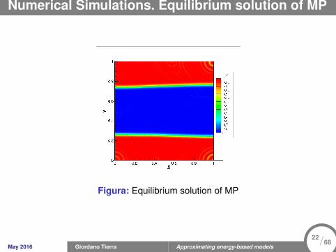
Numerical Simulations. Equilibrium solution of MP
Figura: Equilibrium solution of MP
May 2016 Giordano Tierra Approximating energy-based models
22/68
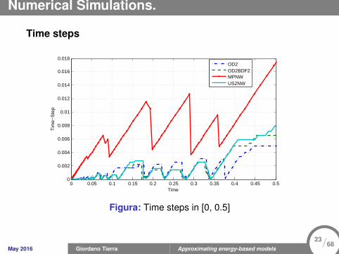
Numerical Simulations.
Time steps
0 0.05 0.1 0.15 0.2 0.25 0.3 0.35 0.4 0.45 0.50
0.002
0.004
0.006
0.008
0.01
0.012
0.014
0.016
0.018
Time
Tim
e−S
tep
OD2OD2BDF2MPNWUS2NW
Figura: Time steps in [0, 0.5]
May 2016 Giordano Tierra Approximating energy-based models
23/68
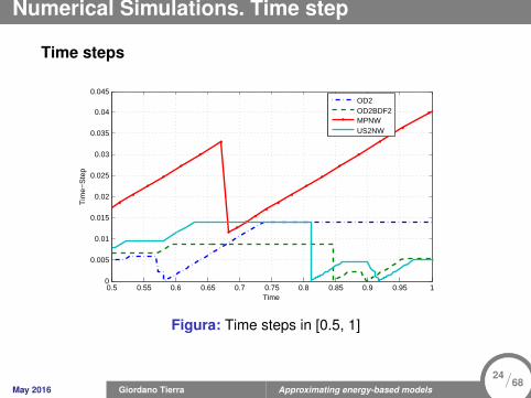
Numerical Simulations. Time step
Time steps
0.5 0.55 0.6 0.65 0.7 0.75 0.8 0.85 0.9 0.95 10
0.005
0.01
0.015
0.02
0.025
0.03
0.035
0.04
0.045
Time
Tim
e−S
tep
OD2OD2BDF2MPNWUS2NW
Figura: Time steps in [0.5, 1]
May 2016 Giordano Tierra Approximating energy-based models
24/68
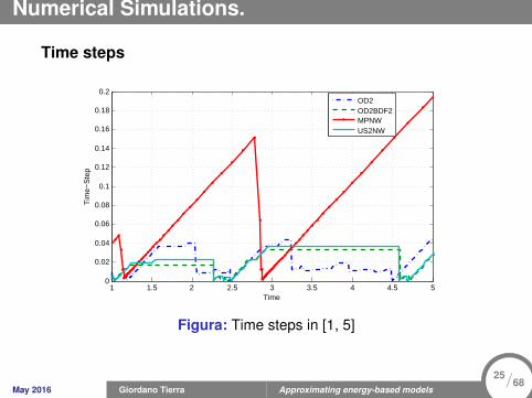
Numerical Simulations.
Time steps
1 1.5 2 2.5 3 3.5 4 4.5 50
0.02
0.04
0.06
0.08
0.1
0.12
0.14
0.16
0.18
0.2
Time
Tim
e−S
tep
OD2OD2BDF2MPNWUS2NW
Figura: Time steps in [1, 5]
May 2016 Giordano Tierra Approximating energy-based models
25/68
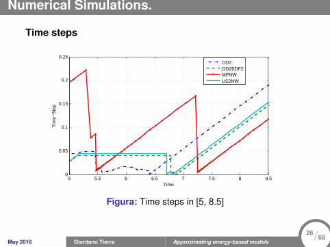
Numerical Simulations.
Time steps
5 5.5 6 6.5 7 7.5 8 8.50
0.05
0.1
0.15
0.2
0.25
Time
Tim
e−S
tep
OD2OD2BDF2MPNWUS2NW
Figura: Time steps in [5, 8.5]
May 2016 Giordano Tierra Approximating energy-based models
26/68
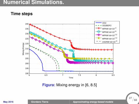
Numerical Simulations.
Time steps
6 6.5 7 7.5 8 8.5190
195
200
205
210
215
220
225
230
235
240
Time
Mix
ing
Ene
rgy
OD2OD2BDF2
MPNW tol=10−3
MPNW tol=10−8
MPNW tol=10−12
MPNW tol=10−13
US2NW tol=10−8
Figura: Mixing energy in [6, 8.5]
May 2016 Giordano Tierra Approximating energy-based models
27/68
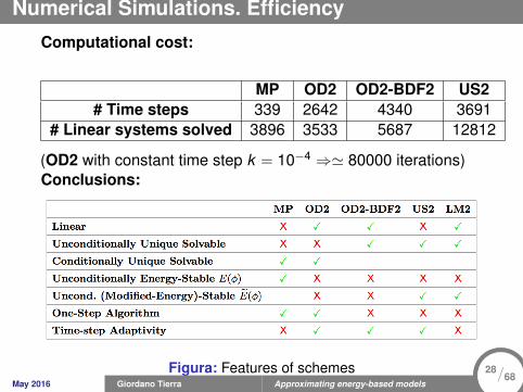
Numerical Simulations. Efficiency
Computational cost:
MP OD2 OD2-BDF2 US2# Time steps 339 2642 4340 3691
# Linear systems solved 3896 3533 5687 12812
(OD2 with constant time step k = 10−4 ⇒' 80000 iterations)Conclusions:
Figura: Features of schemesMay 2016 Giordano Tierra Approximating energy-based models
28/68
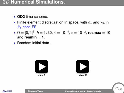
3D Numerical Simulations.
• OD2 time scheme.• Finite element discretization in space, with φh and wh inP1-cont. FE
• Ω = [0,1]3, h = 1/30, γ = 10−4, ε = 10−2, resmax = 10and resmin = 1.
• Random initial data.
May 2016 Giordano Tierra Approximating energy-based models
29/68
Applications
LINEAR UNCONDITIONAL ENERGY-STABLE SPLITTINGSCHEMES FOR A PHASE-FIELD MODEL FORNEMATIC-ISOTROPIC FLOWS WITH ANCHORING EFFECTS
May 2016 Giordano Tierra Approximating energy-based models
30/68
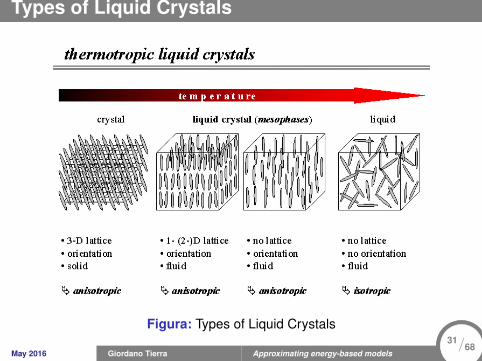
Types of Liquid Crystals
Figura: Types of Liquid Crystals
May 2016 Giordano Tierra Approximating energy-based models
31/68
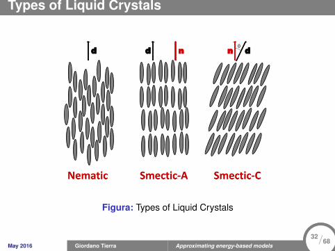
Types of Liquid Crystals
d d n d n
θ
Nematic Smectic-A Smectic-C
Figura: Types of Liquid Crystals
May 2016 Giordano Tierra Approximating energy-based models
32/68
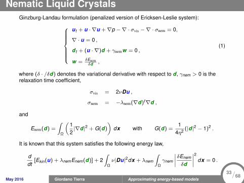
Nematic Liquid CrystalsGinzburg-Landau formulation (penalized version of Ericksen-Leslie system):
ut + u · ∇u +∇p −∇ · σvis −∇ · σnem = 0,
∇ · u = 0 ,
d t + (u · ∇)d + γnemw = 0 ,
w = δEnemδd ,
(1)
where (δ · /δd) denotes the variational derivative with respect to d , γnem > 0 is therelaxation time coefficient,
σvis = 2νDu ,
σnem = −λnem(∇d)t∇d ,
and
Enem(d) =
∫Ω
(12|∇d |2 + G(d)
)dx with G(d) =
14η2
(|d |2 − 1)2 .
It is known that this system satisfies the following energy law,
ddt
[Ekin(u) + λnemEnem(d)] + 2∫
Ων|Du|2dx + λnem
∫Ωγnem
∣∣∣∣ δEnem
δd
∣∣∣∣2 dx = 0 .
May 2016 Giordano Tierra Approximating energy-based models
33/68
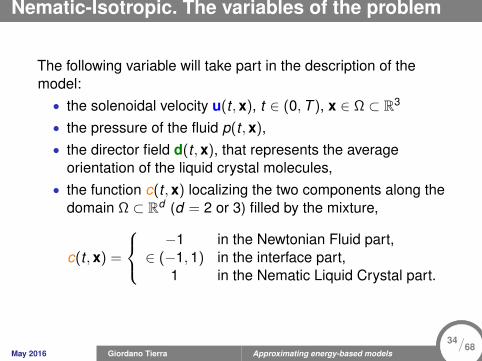
Nematic-Isotropic. The variables of the problem
The following variable will take part in the description of themodel:• the solenoidal velocity u(t ,x), t ∈ (0,T ), x ∈ Ω ⊂ R3
• the pressure of the fluid p(t ,x),• the director field d(t ,x), that represents the average
orientation of the liquid crystal molecules,• the function c(t ,x) localizing the two components along the
domain Ω ⊂ Rd (d = 2 or 3) filled by the mixture,
c(t ,x) =
−1 in the Newtonian Fluid part,
∈ (−1,1) in the interface part,1 in the Nematic Liquid Crystal part.
May 2016 Giordano Tierra Approximating energy-based models
34/68
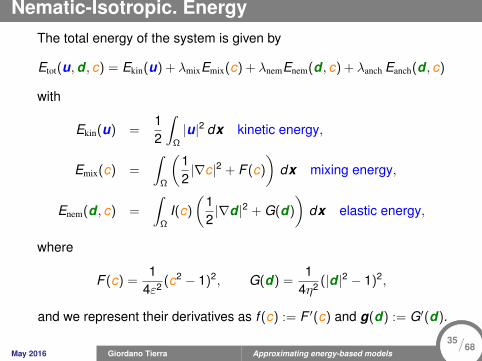
Nematic-Isotropic. EnergyThe total energy of the system is given by
Etot(u,d , c) = Ekin(u) + λmixEmix(c) + λnemEnem(d , c) + λanch Eanch(d , c)
with
Ekin(u) =12
∫Ω
|u|2 dx kinetic energy,
Emix(c) =
∫Ω
(12|∇c|2 + F (c)
)dx mixing energy,
Enem(d , c) =
∫Ω
I(c)
(12|∇d |2 + G(d)
)dx elastic energy,
where
F (c) =1
4ε2 (c2 − 1)2, G(d) =1
4η2 (|d |2 − 1)2,
and we represent their derivatives as f (c) := F ′(c) and g(d) := G′(d).
May 2016 Giordano Tierra Approximating energy-based models
35/68

Nematic-Isotropic. The anchoring effect
At the interface between the nematic and newtonian fluids, liquidcrystals prefer to orientate following a certain direction (called aseasy direction).Three effects can be described:• the parallel case, where the director vector is parallel to the
interface,• the homeotropic case, where the director vector is normal to
the interface,• no anchoring.
NO ANCHORING
PARALLEL ANCHORING
HOMEOTROPIC ANCHORING
May 2016 Giordano Tierra Approximating energy-based models
36/68
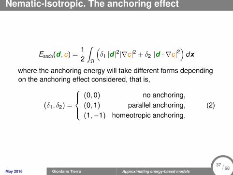
Nematic-Isotropic. The anchoring effect
Eanch(d , c) =12
∫Ω
(δ1 |d |2|∇c|2 + δ2 |d · ∇c|2
)dx
where the anchoring energy will take different forms dependingon the anchoring effect considered, that is,
(δ1, δ2) =
(0,0) no anchoring,(0,1) parallel anchoring,(1,−1) homeotropic anchoring.
(2)
May 2016 Giordano Tierra Approximating energy-based models
37/68
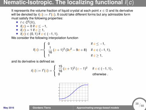
Nematic-Isotropic. The localizing functional I(c)It represents the volume fraction of liquid crystal at each point x ∈ Ω and its derivativewill be denoted by i(c) := I′(c). It could take different forms but any admissible formmust satisfy the following properties:• I ∈ C2(R),• I(c) = 0 if c ≤ −1,• I(c) = 1 if c ≥ 1,• I(c) ∈ (0, 1) if c ∈ (−1, 1).
We consider the following interpolation function
I(c) :=
0 if c ≤ −1,116
(c + 1)3 (3c2 − 9c + 8) if c ∈ (−1, 1),
1 if c ≥ 1,
and its derivative is defined as
i(c) := I′(c) =
1516
(c + 1)2 (c − 1)2 if c ∈ (−1, 1) ,
0 otherwise .
−1 −0.8 −0.6 −0.4 −0.2 0 0.2 0.4 0.6 0.8 1
0
0.2
0.4
0.6
0.8
1
x
Figura: Interpolator I(c) in interval [0,1]May 2016 Giordano Tierra Approximating energy-based models
38/68
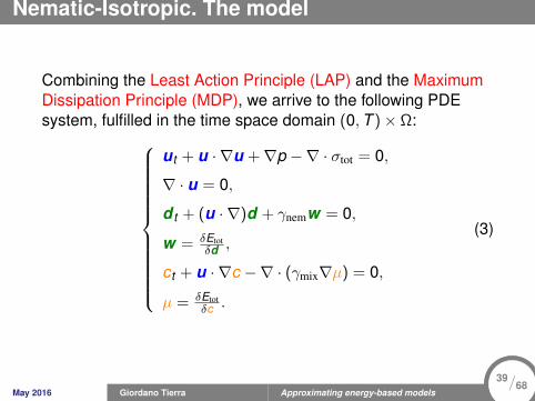
Nematic-Isotropic. The model
Combining the Least Action Principle (LAP) and the MaximumDissipation Principle (MDP), we arrive to the following PDEsystem, fulfilled in the time space domain (0,T )× Ω:
ut + u · ∇u +∇p −∇ · σtot = 0,
∇ · u = 0,
d t + (u · ∇)d + γnemw = 0,
w = δEtotδd ,
ct + u · ∇c −∇ · (γmix∇µ) = 0,
µ = δEtotδc .
(3)
May 2016 Giordano Tierra Approximating energy-based models
39/68
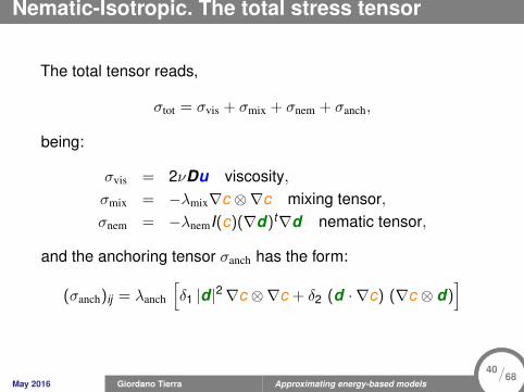
Nematic-Isotropic. The total stress tensor
The total tensor reads,
σtot = σvis + σmix + σnem + σanch,
being:
σvis = 2νDu viscosity,σmix = −λmix∇c ⊗∇c mixing tensor,σnem = −λnemI(c)(∇d)t∇d nematic tensor,
and the anchoring tensor σanch has the form:
(σanch)ij = λanch
[δ1 |d |2∇c ⊗∇c + δ2 (d · ∇c) (∇c ⊗ d)
]
May 2016 Giordano Tierra Approximating energy-based models
40/68
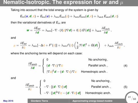
Nematic-Isotropic. The expression for w and µ
Taking into account that the total energy of the system is given by
Etot(u,d , c) = Ekin(u) + λmixEmix(c) + λnemEnem(d , c) + λanch Eanch(d , c)
then the variational derivatives of Etot are
w =δEtot
δd= λnem[−∇ · (I(c)∇d) + I(c) G′(d)] + λanch
δEanch
δd,
and
µ =δEtot
δc= λmix[−∆c + F ′(c)] + λnemI′(c)
(12|∇d |2 + G(d)
)+ λanch
δEanch
δc,
where the anchoring terms will depend on each case:
δEanch
δd=
0 No anchoring ,
(d · ∇c)∇c Parallel anch. ,
|∇c|2d − (d · ∇c)∇c Homeotropic anch. .
(4)
and
δEanch
δc=
0 No anchoring ,
−∇ · [(d · ∇c) d] Parallel anch. ,
−∇ · [|d |2∇c − (d · ∇c) d] Homeotropic anch.
(5)
May 2016 Giordano Tierra Approximating energy-based models
41/68
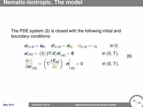
Nematic-Isotropic. The model
The PDE system (3) is closed with the following initial andboundary conditions:
u|t=0 = u0, d |t=0 = d0, c|t=0 = c0 in Ω,
u|∂Ω =(I(c)∇d
)n∣∣∂Ω
= 0 in (0,T ),
∂c∂n
∣∣∣∣∂Ω
=
(∇δEtot
δc
)· n∣∣∣∣∂Ω
= 0 in (0,T ),
(6)
May 2016 Giordano Tierra Approximating energy-based models
42/68
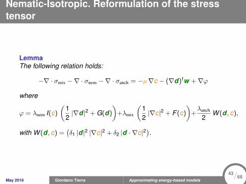
Nematic-Isotropic. Reformulation of the stresstensor
LemmaThe following relation holds:
−∇ · σmix −∇ · σnem −∇ · σanch = −µ∇c − (∇d)tw +∇ϕ
where
ϕ = λnem I(c)
(12|∇d |2 + G(d)
)+λmix
(12|∇c|2 + F (c)
)+λanch
2W (d , c),
with W (d , c) =(δ1 |d |2 |∇c|2 + δ2 |d · ∇c|2
).
May 2016 Giordano Tierra Approximating energy-based models
43/68
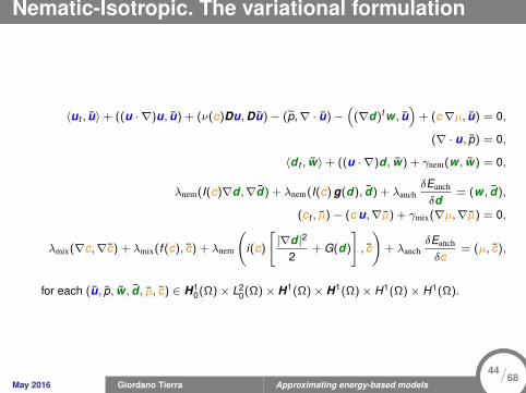
Nematic-Isotropic. The variational formulation
〈ut , u〉+ ((u · ∇)u, u) + (ν(c)Du,Du)− (p,∇ · u)−(
(∇d)t w , u)
+ (c∇µ, u) = 0,
(∇ · u, p) = 0,
〈d t , w〉+ ((u · ∇)d , w) + γnem(w , w) = 0,
λnem(I(c)∇d ,∇d) + λnem(I(c) g(d), d) + λanchδEanch
δd= (w , d),
(ct , µ)− (c u,∇µ) + γmix(∇µ,∇µ) = 0,
λmix(∇c,∇c) + λmix(f (c), c) + λnem
(i(c)
[|∇d |2
2+ G(d)
], c
)+ λanch
δEanch
δc= (µ, c),
for each (u, p, w , d , µ, c) ∈ H10(Ω)× L2
0(Ω)× H1(Ω)× H1(Ω)× H1(Ω)× H1(Ω).
May 2016 Giordano Tierra Approximating energy-based models
44/68
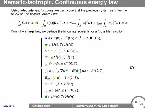
Nematic-Isotropic. Continuous energy lawUsing adequate test functions, we can prove that the previous system satisfies thefollowing (dissipative) energy law:
ddt
Etot(u,d , c) +
∫Ων(c)|Du|2 dx + γnem
∫Ω|w |2 dx + γmix
∫Ω|∇µ|2 dx = 0.
From the energy law, we deduce the following regularity for a (possible) solution:
u ∈ L∞(0,T ; L2(Ω)) ∩ L2(0,T ; H1(Ω)),
w ∈ L2(0,T ; L2(Ω)),
∇c ∈ L∞(0,T ; L2(Ω)),
∇µ ∈ L2(0,T ; L2(Ω)),∫Ω F (c)dx ∈ L∞(0,T ),∫Ω I(c)
(12 |∇d |2 + G(d)
)dx ∈ L∞(0,T )
Eanch(c,d) ∈ L∞(0,T ),
c ∈ L∞(0,T ; H1(Ω)),∫Ω I(c) |d |4 ∈ L∞(0,T ),
d ∈ L∞(0,T ; L2(Ω)).
(7)
May 2016 Giordano Tierra Approximating energy-based models
45/68
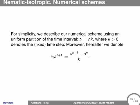
Nematic-Isotropic. Numerical schemes
For simplicity, we describe our numerical scheme using anuniform partition of the time interval: tn = nk , where k > 0denotes the (fixed) time step. Moreover, hereafter we denote
δtan+1 :=an+1 − an
k.
May 2016 Giordano Tierra Approximating energy-based models
46/68
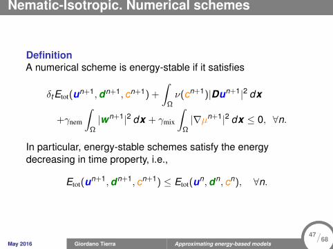
Nematic-Isotropic. Numerical schemes
DefinitionA numerical scheme is energy-stable if it satisfies
δtEtot(un+1,dn+1, cn+1) +
∫Ων(cn+1)|Dun+1|2 dx
+γnem
∫Ω|wn+1|2 dx + γmix
∫Ω|∇µn+1|2 dx ≤ 0, ∀n.
In particular, energy-stable schemes satisfy the energydecreasing in time property, i.e.,
Etot(un+1,dn+1, cn+1) ≤ Etot(un,dn, cn), ∀n.
May 2016 Giordano Tierra Approximating energy-based models
47/68
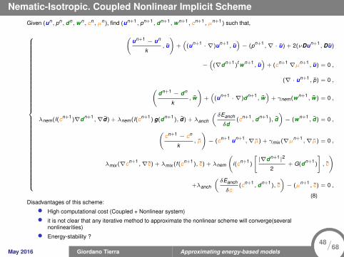
Nematic-Isotropic. Coupled Nonlinear Implicit Scheme
Given (un, pn, dn,wn, cn, µn), find (un+1, pn+1, dn+1,wn+1, cn+1, µn+1) such that,
(un+1 − un
k, u
)+(
(un+1 · ∇)un+1, u)− (pn+1
,∇ · u) + 2(νDun+1,Du)
−(
(∇dn+1)t wn+1, u)
+ (cn+1∇µn+1, u) = 0 ,
(∇ · un+1, p) = 0 ,(dn+1 − dn
k, w
)+(
(un+1 · ∇)dn+1, w)
+ γnem(wn+1, w) = 0 ,
λnem(I(cn+1)∇dn+1,∇d) + λnem(I(cn+1) g(dn+1), d) + λanch
(δEanch
δd(cn+1
, dn+1), d)− (wn+1
, d) = 0 ,
(cn+1 − cn
k, µ
)− (cn+1 un+1
,∇µ) + γmix (∇µn+1,∇µ) = 0 ,
λmix (∇cn+1,∇c) + λmix (f (cn+1), c) + λnem
(i(cn+1)
[|∇dn+1|2
2+ G(dn+1)
], c
)
+λanch
(δEanch
δc(cn+1
, dn+1), c)− (µn+1
, c) = 0 ,
(8)Disadvantages of this scheme:
• High computational cost (Coupled + Nonlinear system)• it is not clear that any iterative method to approximate the nonlinear scheme will converge(several
nonlinearities)• Energy-stability ?
May 2016 Giordano Tierra Approximating energy-based models
48/68

Nematic-Isotropic. Splitting schemes
We have designed two splitting first-order schemes, denoted by
(dn+1,wn+1) → (cn+1, µn+1) → (un+1,pn+1),
or
(cn+1, µn+1) → (dn+1,wn+1) → (un+1,pn+1),
decoupling computations for nematic part (d ,w) from thephase-field part (c, µ) (or the contrary in the second case) andfrom the fluid part (u,p).
May 2016 Giordano Tierra Approximating energy-based models
49/68
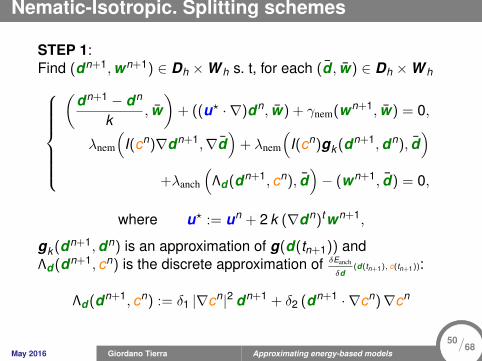
Nematic-Isotropic. Splitting schemes
STEP 1:Find (dn+1,wn+1) ∈ Dh ×W h s. t, for each (d , w) ∈ Dh ×W h
(dn+1 − dn
k, w)
+ ((u? · ∇)dn, w) + γnem(wn+1, w) = 0,
λnem
(I(cn)∇dn+1,∇d
)+ λnem
(I(cn)gk (dn+1,dn), d
)+λanch
(Λd (dn+1, cn), d
)− (wn+1, d) = 0,
where u? := un + 2 k (∇dn)twn+1,
gk (dn+1,dn) is an approximation of g(d(tn+1)) andΛd (dn+1, cn) is the discrete approximation of δEanch
δd(d(tn+1), c(tn+1)):
Λd (dn+1, cn) := δ1 |∇cn|2 dn+1 + δ2 (dn+1 · ∇cn)∇cn
May 2016 Giordano Tierra Approximating energy-based models
50/68
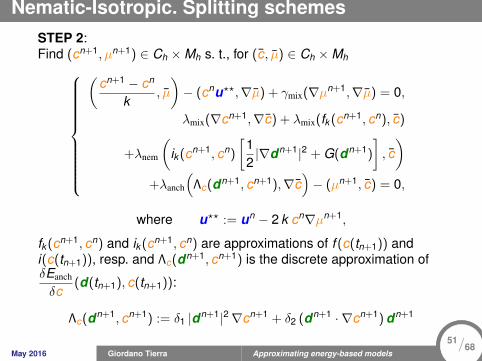
Nematic-Isotropic. Splitting schemesSTEP 2:Find (cn+1, µn+1) ∈ Ch ×Mh s. t., for (c, µ) ∈ Ch ×Mh
(cn+1 − cn
k, µ
)− (cnu??,∇µ) + γmix(∇µn+1,∇µ) = 0,
λmix(∇cn+1,∇c) + λmix(fk (cn+1, cn), c)
+λnem
(ik (cn+1, cn)
[12|∇dn+1|2 + G(dn+1)
], c)
+λanch
(Λc(dn+1, cn+1),∇c
)− (µn+1, c) = 0,
where u?? := un − 2 k cn∇µn+1,
fk (cn+1, cn) and ik (cn+1, cn) are approximations of f (c(tn+1)) andi(c(tn+1)), resp. and Λc(dn+1, cn+1) is the discrete approximation ofδEanch
δc(d(tn+1), c(tn+1)):
Λc(dn+1, cn+1) := δ1 |dn+1|2∇cn+1 + δ2 (dn+1 · ∇cn+1) dn+1
May 2016 Giordano Tierra Approximating energy-based models
51/68
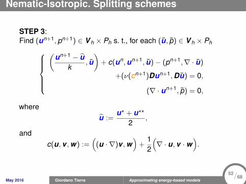
Nematic-Isotropic. Splitting schemes
STEP 3:Find (un+1,pn+1) ∈ V h × Ph s. t., for each (u, p) ∈ V h × Ph
(un+1 − u
k, u)
+ c(un,un+1, u)− (pn+1,∇ · u)
+(ν(cn+1)Dun+1,Du) = 0,
(∇ · un+1, p) = 0,
whereu :=
u? + u??
2,
andc(u,v ,w) :=
((u · ∇)v ,w
)+
12
(∇ · u,v ·w
).
May 2016 Giordano Tierra Approximating energy-based models
52/68
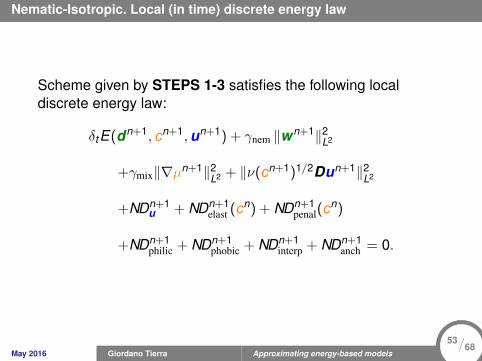
Nematic-Isotropic. Local (in time) discrete energy law
Scheme given by STEPS 1-3 satisfies the following localdiscrete energy law:
δtE(dn+1, cn+1,un+1) + γnem ‖wn+1‖2L2
+γmix‖∇µn+1‖2L2 + ‖ν(cn+1)1/2Dun+1‖2L2
+NDn+1u + NDn+1
elast (cn) + NDn+1penal(c
n)
+NDn+1philic + NDn+1
phobic + NDn+1interp + NDn+1
anch = 0.
May 2016 Giordano Tierra Approximating energy-based models
53/68
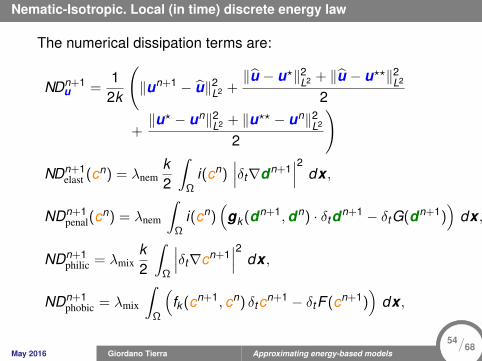
Nematic-Isotropic. Local (in time) discrete energy law
The numerical dissipation terms are:
NDn+1u =
12k
(‖un+1 − u‖2L2 +
‖u − u?‖2L2 + ‖u − u??‖2L2
2
+‖u? − un‖2L2 + ‖u?? − un‖2L2
2
)
NDn+1elast (cn) = λnem
k2
∫Ω
i(cn)∣∣∣δt∇dn+1
∣∣∣2 dx ,
NDn+1penal(c
n) = λnem
∫Ω
i(cn)(
gk (dn+1,dn) · δtdn+1 − δtG(dn+1))
dx ,
NDn+1philic = λmix
k2
∫Ω
∣∣∣δt∇cn+1∣∣∣2 dx ,
NDn+1phobic = λmix
∫Ω
(fk (cn+1, cn) δtcn+1 − δtF (cn+1)
)dx ,
May 2016 Giordano Tierra Approximating energy-based models
54/68
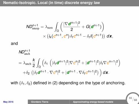
Nematic-Isotropic. Local (in time) discrete energy law
NDn+1interp = λnem
∫Ω
(|∇dn+1|2
2+ G(dn+1)
)×(ik (cn+1, cn) δtcn+1 − δt I(cn+1)
)dx ,
and
NDn+1anch
= λanchk2
∫Ω
(δ1
(|δtdn+1|2|∇cn|2 + |dn+1|2|δt∇cn+1|2
)+δ2
(|δtdn+1 · ∇cn|2 + |dn+1 · ∇δtcn+1|2
) )dx .
with (δ1, δ2) defined in (2) depending on the type of anchoring.
May 2016 Giordano Tierra Approximating energy-based models
55/68
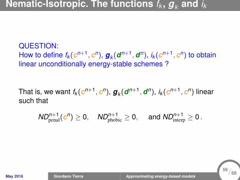
Nematic-Isotropic. The functions fk , gk and ik
QUESTION:How to define fk (cn+1, cn), gk (dn+1,dn), ik (cn+1, cn) to obtainlinear unconditionally energy-stable schemes ?
That is, we want fk (cn+1, cn), gk (dn+1,dn), ik (cn+1, cn) linearsuch that
NDn+1penal(c
n) ≥ 0, NDn+1phobic ≥ 0, and NDn+1
interp ≥ 0 .
May 2016 Giordano Tierra Approximating energy-based models
56/68
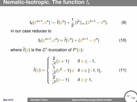
Nematic-Isotropic. The function fk
fk (cn+1, cn) := f (cn) +12‖f ′‖∞ (cn+1 − cn), (9)
in our case reduces to
fk (cn+1, cn) = f (cn) + (cn+1 − cn) (10)
where f (c) is the C1-truncation of F ′(c):
f (c) =
2ε2 (c + 1) if c ≤ −1,
1ε2 (c2 − 1) c if c ∈ [−1,1],
2ε2 (c − 1) if c ≥ 1,
(11)
May 2016 Giordano Tierra Approximating energy-based models
57/68

Nematic-Isotropic. The functions gk and ik
gk (dn+1,dn) = g(dn) +
√512
(dn+1 − dn), (12)
where g(d) is the C1-truncation of g(d):
g(d) =
2 (|d | − 1)d|d |
if |d | ≥ 1,
(|d |2 − 1) d if |d | ≤ 1,
and we also take
ik (cn+1, cn) = i(cn) +5√
312
(cn+1 − cn). (13)
May 2016 Giordano Tierra Approximating energy-based models
58/68
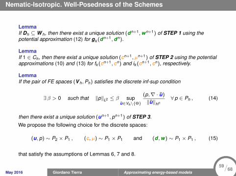
Nematic-Isotropic. Well-Posedness of the Schemes
LemmaIf Dh ⊆ W h, then there exist a unique solution (dn+1,wn+1) of STEP 1 using thepotential approximation (12) for gk (dn+1,dn).
LemmaIf 1 ∈ Ch, then there exist a unique solution (cn+1, µn+1) of STEP 2 using the potentialapproximations (10) and (13) for fk (cn+1, cn) and ik (cn+1, cn), respectively.
LemmaIf the pair of FE spaces (V h,Ph) satisfies the discrete inf-sup condition
∃β > 0 such that ‖p‖L2 ≤ β supu∈Vh\Θ
(p,∇ · u)
‖u‖H1∀ p ∈ Ph , (14)
then there exist a unique solution (un+1, pn+1) of STEP 3.
We propose the following choice for the discrete spaces:
(u, p) ∼ P2 × P1 , (c, µ) ∼ P1 × P1 and (d ,w) ∼ P1 × P1 , (15)
that satisfy the assumptions of Lemmas 6, 7 and 8.
May 2016 Giordano Tierra Approximating energy-based models
59/68
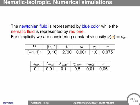
Nematic-Isotropic. Numerical simulations
The newtonian fluid is represented by blue color while thenematic fluid is represented by red one.For simplicity we are considering constant viscosity ν(c) = ν0.
Ω [0,T ] h dt ν0 η
[−1,1]2 [0,10] 2/90 0,001 1,0 0,075
λnem λmix λanch γnem γmix ε
0,1 0,01 0,1 0,5 0,01 0,05
May 2016 Giordano Tierra Approximating energy-based models
60/68
Nematic-Isotropic. Circular droplet and directorfield parallel to the y-axis
May 2016 Giordano Tierra Approximating energy-based models
61/68
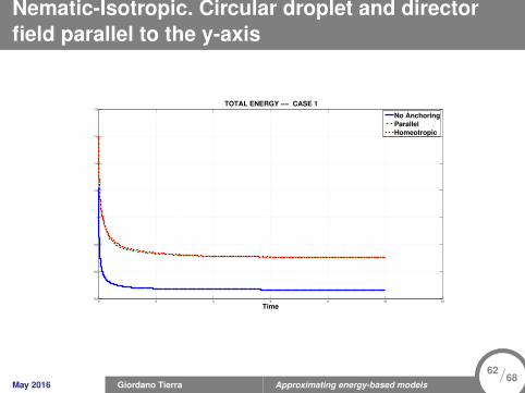
Nematic-Isotropic. Circular droplet and directorfield parallel to the y-axis
0 2 4 6 8 10 120.4
0.6
0.8
1
1.2
1.4
1.6
1.8
Time
TOTAL ENERGY −− CASE 1
No Anchoring
Parallel
Homeotropic
May 2016 Giordano Tierra Approximating energy-based models
62/68
Nematic-Isotropic. Elliptic droplet with two pointsdefects at (±1/2,0)
• A Hedgehog defect at (1/2,0) and an Antihedgehog defectat (−1/2,0)
d0(x) = d/√|d |2 + 0,052, with d = (x2 + y2 − 0,25, y) .
Defect annihilation in Nematic Liquid Crystals
Defect annihilation in Nematic Liquid Crystals Drops
May 2016 Giordano Tierra Approximating energy-based models
63/68
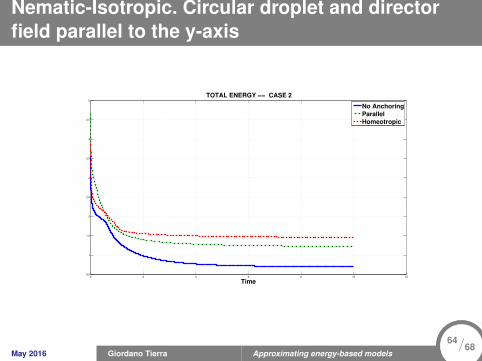
Nematic-Isotropic. Circular droplet and directorfield parallel to the y-axis
0 2 4 6 8 10 120.5
1
1.5
2
2.5
3
3.5
4
4.5
5
Time
TOTAL ENERGY −− CASE 2
No Anchoring
Parallel
Homeotropic
May 2016 Giordano Tierra Approximating energy-based models
64/68
Nematic-Isotropic. Spinodal Decomposition
• Random initial data for c, i.e., c ∈ [−10−2,10−2] inΩ = [0,1]× [0,1], t ∈ [0,1] and dt = 10−4.
• The initial director vector is computed using the function:
d = I(c)(
sin(x y) sin(x y), cos(x y) cos(x y)).
May 2016 Giordano Tierra Approximating energy-based models
65/68
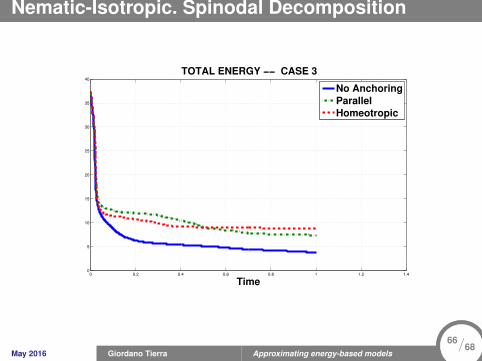
Nematic-Isotropic. Spinodal Decomposition
0 0.2 0.4 0.6 0.8 1 1.2 1.40
5
10
15
20
25
30
35
40
Time
TOTAL ENERGY −− CASE 3
No Anchoring
Parallel
Homeotropic
May 2016 Giordano Tierra Approximating energy-based models
66/68
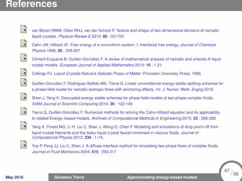
References
van Bijnen RMW, Otten RHJ, van der Schoot P. Texture and shape of two-dimensional domains of nematicliquid crystals. Physical Review E 2012; 86 : 051703
Cahn JW, Hilliard JE. Free energy of a nonuniform system. I. Interfacial free energy. Journal of ChemicalPhysics 1958; 28 : 258-267
Climent-Ezquerra B, Guillén-González F. A review of mathematical analysis of nematic and smectic-A liquidcrystal models. European Journal of Applied Mathematics 2013; 10 : 1-21
Collings PJ. Liquid Crystals:Nature’s Delicate Phase of Matter. Princeton University Press, 1990.
Guillén-González F, Rodríguez-Bellido MA, Tierra G. Linear unconditional energy-stable splitting schemes fora phase-field model for nematic-isotropic flows with anchoring effects. Int. J. Numer. Meth. Engng 2016;
Shen J, Yang X. Decoupled energy stable schemes for phase field models of two-phase complex fluids.SIAM Journal of Scientific Computing 2014; 36 : 122-145
Tierra G, Guillén-González F. Numerical methods for solving the Cahn-Hilliard equation and its applicabilityto related Energy–based models. Archives of Computational Methods in Engineering 2015; 22 : 269-289
Yang X, Forest MG, Li H, Liu C, Shen J, Wang Q, Chen F. Modeling and simulations of drop pinch-off fromliquid crystal filaments and the leaky liquid crystal faucet immersed in viscous fluids. Journal ofComputational Physics 2013; 236 : 1-14,
Yue P, Feng JJ, Liu C, Shen J. A diffuse-interface method for simulating two-phase flows of complex fluids.Journal of Fluid Mechanics 2004; 515 : 293-317
May 2016 Giordano Tierra Approximating energy-based models
67/68

THANK YOU FOR YOUR ATTENTION!
May 2016 Giordano Tierra Approximating energy-based models
68/68