•

•

•

DYNAM/CS OF THE JAROS/TE CONVERSION PROCESS

A THESIS

by

GILLIAN L. HOLCROFT

Department of Chemical Engineering

McGili University, Montréal

March 1994

A Thesis submitted to the Faculty of Graduate Studies and Research

in partial fulfilment of the requirements of the

degree of Master of Engineering

(c) Gillian Holcroft 1994

•

•

•

Abstract

Canadian Electrolytic Zmc in Valleyfield, Québec utilizes the conventional Roast­

Leach-Electrowin process to produce zinc metal. Iron remCJval is carried out in the

jarosite conversion circuit which consists ot ten continuous stirred tank reactors in

series.

ln thls study, the tirst five tanks of thE: jarosite conversion circuit were piloted and

process identification experiments were carried out. Step changes in the fJows of

the raw acid, spent aCld, jaroslte slurry and zinc ferrite slurry streams were

performed. The goal ot these experiments was to collect transient response data

which cou Id be used to validate a dynamic conversion circuit modal. The process

was found to be most sensitive to changes in the flow of the raw acid stream.

The zinc ferrite dissolution rate constant calculated from the experimental data

agrees with literature values. Using a jarosite precipitation rate expression trom

the literature, it was found that jarosite precipitation is negligible in the tirst reactor

but cannot be ignored in the second tank.

The dynamlc model provides a good representation of the tirst two tanks of the

jarosite conversion circuit and can be used for both process control and

optimization studies on a full-scale facility .

•

•

•

Zinc Électrolytique du Canada (ValieyfiBld, Québec) utilise le procédé

conventionnel: Grillage-lixiviation-ÉlectrolysE! pour produire du zinc. L'enlèvement

de fer dans le circuit de conversion avec jarosite est effectué dans un régime de

dix réservoirs continus agités en série.

Dans cette étude, les cinq premiers réservoirs du circuit de conversion avec

jarosite ont été étudiés à l'échelle pilote et des e:<périences permettant

l'identification des paramètres du procédé onl été effectuées. Des changements

de type échelon ont été appliqués sur les débits de: acide brut, éléctrolyte, pulpe

de jarosite, et pulpe des farrites de zinc. Ces expériences avaient pour but

d'obtenir des données en régime transitoire et ensUite de permettre la validation

d'un modèle dynamique du circuit de COnVE:lrSlon. Les changements de débit sur

le courant d'acide brut ont eu le plus gland 13ffet sur le procédé.

Le taux de dissolution de la ferrite de zinc calculé à partir des données

expérimenta.les est en accord avec les données disponibles dans la littérature.

L'utilisation d'un taux de précipitation de la jarosite tiré de la littérature a permis da

montrer que la précipitation de la jarosite est négligeable dans le premier réservoir

mais significative dans le second.

Le modèle dynamique obtenu Ct permis d'obtenir une II1dication fiable du

comportement des deux premiers réservoirs du circuit de conversion avec jarosite.

Ce modèle sera utilisé pour étudier les stratégies de contrôle et d'optimisation du

procédé existant.

•

•

•

Acknowleclgements

1 would like to thank the Noranda Technology Centre for supporting this work, and

more specifically Lucy Rosata fOi her tl3chnical guidance throughout this prc>ject

and for helping put together its original concept. Without her ability for ma,king

people challenge themselves, this project would never have been initiated. 1 wc)uld

also like to thank Robert Stanley who authorized Noranda's support for this studl/.

This work was performed with the fil1ancial assistanCE! received from an NSëRC

scholarship for employed scientists and engineers.

Invaluable guidanCE: was received from my supervisor Dr. Dimitrios Berk, especially

with the detailed chemical reaction engineering aspects of this work. Dr. Michel

Perrier, who co-supervised this thesis, provided direction during the project's

conception and with the process control portion of this study .

1 was tortunate to get assistance with the pilot experiments from a very bright and

energetic student from Sherbrooke University, Chantal Goyette. The large amount

of data that was generated after each experiment was pul into an understandable

format and plotted with the help of my sister, Carolyn, and J thank her very much.

Finally,l would like to thanh l1y husband, Paul for his continuai support as weil as

the rest of my family for their understanding during my studies .

•

•

•

Table of Contents Page

Chapter 1 General Introduction

1.1 Jarosite Conversion Process ... . . . . . . . . . . . . . . . . . . . . . .. 1

1.2 Canadian Electrolytic Zinc's Conversion Process . . . . . . . . . . .. 3

1.3 Process Control Modelling Approaches . . . . . . . . . . . . . . . . . .. 5

1.4 Thesis Objectives .................................. 6

1.5 Thesis Outil ne . .. ................................. 7

Chapter 2 Literature Review

2.1 Process Control & Automation of a Zinc Leaching Circuit ...... 9

2.2 Zinc Ferrite Leaching Kinetics ........................ 10

2.3 Jarosite Precipitation Kinetics . . . . . . . . . . . . . . . . . . . . . . . .. 16

Chapter 3 Experimental Methods

3.1 Overview ....................................... 21

3.2 Pilot Equipment . . . . . . . . . . . . . . . . . . . . . . . . . . . . . . . . . .. 21

3.3 Operating Procedure. . . . . . . . . . . . . . . . . . . . . . . . . . . . . .. 29

3.4 Error Analysis . . . . . . . . . . . . . . . . . . . . . . . . . . . . . . . . . . .. 33

Chapter 4 Experimental Results

4.1 Parameters Investigated ............................ 39

4.2 Mass Balances for First Reactor . . . . . . . . . . . . . . . . . . . . . .. 42

4.3 Statistical Analysis . . . . . . . . . . . . . . . . . . . . . . . . . . . . . . . .. 51

4.4 Determination of Rate Constant . . . . . . . . . . . . . . . . . . . . . .. 55

4.5 Process Identification from Step Responses .............. 57

4.6 DiSCUSSion of Tank 1 Results ....................... " 60

•

•

•

Page

Chapter 5 Dynamic Model

5.1 Determimstic Dynamic Madel . . . . . . . . . . . . . . . . . . . . . . . .. 62

5.1.1 Incorporation of the Rate Equations .... . . . . . . . . . .. 65

5.1.2 Tank 1 Transient Model . . . . . . . . . . . . . . . . . . . . . . .. 67

5.2 Process Simulation Results

5.2.1 Tank 1 Results ............................. 70

5.2.2 Tank 1 Jarosite Rate Constant Stability . . . . . . . . . . .. 76

5.2.3 Tank 2 Results ............................. 77

5.4 Process Control Strategy . . . . . . . . . . . . . . . . . . . . . . . . . . .. 82

Chapter 6 Conclusion

6.1 Conclusion .... . . . . . . . . . . . . . . . . . . . . . . . . . . . . . . . . .. 84

6.2 Proposai for Future Studles ... . . . . . . . . . . . . . . . . . . . . . .. 85

Chapter 7 References . . . . . . . . . . . . . . . . . . . . . . . . . . . . . . . . . .. 86

•

•

•

APPENDIX 1

APPENDIX Il

APPENDIX III

APPENDIX IV

APPENDIX V

APPENDIX VI

APPENDIX VII

APPENDIX VIII

Appendiçes

Nomenclature

Calibration Curves for Rotameters

Tank Charactensatlon and Tracer Selection Study

Zinc Fernte and Jarosite Solids

Acid Titratlon Method

Test for Comparing the Means of Two Variables

Calculation of the lonic Strength in Tank 1

TANK 1 Assays: Tests B,C,D and E

-------------------------------------------------------

• List of Figures

Chaptdr 1

Figure 1·1 R.L.E. Process

Figure 1-2 CEZrnc Zinc Refmmg Process

Figure 1·3 CEZinc Leaching Ctrcuit

Chapter 3

Figure 3·1 Actual Jarosite Pilot C"cuit

Figure 3-2 Actual Jarosite PIlot Circuit: Vlew of First Tank

Figure 3-3 Pilot Scale Jarosite Circuit

Figure 3-4 Reactor Construction

Figure 3-5 Pilot Plant Instrumentation

• Chapter 4

Figure 4·1 Grouping of Data mto Process States

Figure 4-2 Jarosite Tank 1

Figure 4-3 Process Gam and Tlme Constant Estimation

Chapter 5

Figure 5-1 Jarosite Tank 1

Figure 5-2 TEST B Sulphuric Acid Concentration Changes

Figure 5-3 TEST 0 Sulphuric Acid Concentration Changes

Figure 5-4 TEST E Sulphuric Acid Concentration Changes

Figure 5-5 TEST B Ferric Iron Concentration Changes

Figure 5-6 TEST C Ferric Iron Concentration Changes

Figure 5-7 TEST 0 Zinc ConcentratIOn Changes

Figure 5-8 TEST B Mass FractIOn of Zmc in Solids Changes

• Figure 5-9 TEST C Mass Fraction of Zinc in Solids Changes

•

•

•

Figure 5-10

Figure 5-11

Figure 5-12

Figure 5-13

Figure 5-14

Figure 5-15

Figure 5-16

Figure 5-17

Figure 5-18

Figure 5-19

Figure 5-20

Chapter 5 (continued)

TESï 0 !vlass Fraction of Linc in Solids Changes

TEST f~ Mass FractIOn of Zinc in Solids Changes

TEST E Effect of Jarosite PrecipItation

TEST B Tank 2: Sulphuric Acid Concentration Changes

TEST 0 Tank 2: Sulphunc Acid Concentration Changes

TEST B Tank 2· Ferric Iron Concentration Changes

TEST C Tank 2. Ferric Iron Concentration Changes

TEST D Tank 2: Zmc Concentration Changes

TEST C Tank 2: Mass Fraction of Zinc m Solids Changes

TEST D Tank 2: Mass Fraction of Zinc in Solids Changes

TEST E Tank 2: Mass Fraction of Zinc in Solids Changes

Chapter 6

Figure 6-1 Possible Control Strategy

•

•

•

Table 111-1

Table 111-2

Table 111-3

Table 111-4

Table 111-5

Table IV-1

Table IV-2

Table IV-3

Table IV-4

Table IV-5

Table IV-6a

Table IV-6b

Table IV-7a

Table IV~7b

Table IV-Sa

Table IV-Sb

Table IV-9

Table IV-10

List of Tables

Chapter 3

Feed Stream Flows

.

Comparison of Industrial and Elemental Solid Compositions

Feed Solution Compositions and Densities

Error in I.C.P. Analysis

Error in Flow Measurements

Chapter 4

Step Change Flows

TEST B - Tank 1: Exit Flow

TEST B - Tank 1: Acid Consumption

TEST B - Tank 1: Zinc Mass Balance

Tank 1: Acid Consumed and Solids Leached

Tank 1: Mass Balances for Zinc, Iron, and Lead

Tank 2: Mass Balances for Zinc, Iron, and Lead

Comparison of Initial and Step Change Steady State Acid

Concentrations for Tank 1

Comparison of Initial and Step Change Steady State Iron

Concentrations for Tank 1

Comparison of Initial and Step Change Steady State Iron in

Solids for Tank 1

Comparison of Initial and Step Change Steady State Zinc in

Solids for Tank 1

Reaction Extents and Rate Constants

Process Gains and Time Constants

•

•

•

1

Chapter 1 INTRODUCTION

1.1 Jarosite Conversion Process

Over 75% of commercial zinc is produced via the Roast-Leach-Electrowin (R.L.E.)

process. The general flow-sheet of this process is shown in Figure 1-1. In the

roasting section of this process, the concentrate, which ie composed of zinc and

iron sulfides, is oxidized at 930°C to produce a calcine of mainly zinc oxides (ZnO)

and zinc ferrites (ZnO.Fe20 3). Spent electrolyte, which is high in sulphuric acid,

leaches the calcine under atmospheric conditions to produce a zinc sulphate

solution. This solution IS then electrowinned in the cell-house to produce pure zinc

cathodes. The differences amongst R.L.E. plants lies mainly in the method used

to remove iron trom the zinc sulphate leach solutions. Iron removal is an essential

step in electrowinning flow-sheets since iron interferes with the purification process

and causes problems with the electro-deposition of zinc in the cell house.

OXYGEN CONCENTRA TE SPENT AC l D

TI Il -r(' f;.: Q V L. '-- ~ Il

ROAST CALe l NE LEACH ELECTROWIN > > - - -Zr(-J;4 ! aq) ~ !'" .. 1 - -' ".

IMPURITIES Il Il Fe REMOVAL Il Zn METAL > ;,

Figure 1-1 RLE. Process

The majority of zinc concentrates contain approximately 50% zinc and between 5%

to 12% iron, in which a large portion of the iron is converted to zinc ferrite in the

roaster. The three main methods of iron removal are named ~fter the minerai that

they generate, namely the Hematite, Goethiie and the Jarosite process .

•

•

2

The Jarosite process was developed independèntly in Europe and Australia in the

'60's. The advent of this process, which has many variations (eg. pre

neutralizatlon, multistage leaching ... ), resulted in the ability to separate readily the

dissolved iron trom the zinc solution. Normally the temperature is maintained

between 95 to 100°C, a source of alkali is added, and jarosite seed is recycled to

provide nucleation sites for jarosite crystal growth. One ot the drawbacks of this

process stems tram the nature of its relatively high temperature and corrosive

operating conditions. As a result, the selection of appropriate construction

materials is essential. There is also an environ mental drawback of this process

due ta the large quantity of jarosite that must be disposed of. As an example, a

typical 100 000 tons per year plant will produce 40 000 tons per year jarosite

solids (approximately 73000 tons per year jarosite slurry) which are normally sent

ta tailings ponds. A study is currently under-way at the Noranda Technology

Centre to examine alternative options for iron disposaI.

The difference between the convention al jarosite process and the jarosite

conversion process is in the addition of calcine in the former for acidity control.

The conversion process results in the simultaneous hot acid leaching of zinc

ferrites and in the precipitation of jarosite solids in the same process stage. This

process offers significant capital cost savings but at the expense of any possible

recovery of silver and lead values. This process can achieve both high overall zinc

extractions and zinc recoveries. Although many electrolytic zinc plants have

adopted the jarosite process, only Canadian Electrolytic Zinc (CEZinc) in

Valleyfield, Québec and Outokumpu in Kokkola, Finland employ the jarosite

conversion process.

According to Dutrizac (1), the major control parameters for the conversion process

are acid concentration, which is the key variable, temperature, and the molar ratio

of acid to iron. If the acid concentration is low, iron wilL readily precipitate;

however, high acid concentrations are advantageous for leaching of zinc ferrites.

•

•

•

3

Consequently, the optimizatlon of the conversion process requires the

determination of the most suitable acid level in each stage.

1.2 Canadian Electrolytic Zinc's Conversion Process

Tt-.'d CEZinc plant produces 230 000 tons per year of electrowinned zinc. As seen

in Figure 1-2, the plant IS divided into five main areas: roasting, leaching,

purification, electrolysis and casting. The jarosite conversion circuit is in the

leaching section of the plant. This circuit consists of ten continuous stirred tank

reactors in series as shown in Figure 1-3.

CONCENTRA TE SPENT AC ID

ij ~ Il Bo.",", LEACH '.'UO'lpURIFN.I'uo"", ELECTROWIN SOLN. SOLN.

IRON /1 J ij Zn CATHODE

REMOVAL ,.'UO"", ~ IJAROSITE)

Zn METAL CASTING Q

Figure 1-2 CEZinc Zinc Refining Process

The following are the two main reactions occurring in the conversion circuit:

Zinc Ferrite leaching:

Zno.Fe2 0 3 (s) + aH' -7 Zn 2+ + 2Fe 3

+ + 4H20(aq) (1.1)

Ammonium Jarosite Precipitation:

The purpose of the jarosite conversion circuit is to extract the zinc from the zinc

ferrite solids and to dispose of the iron as insoluble ammonium jarosite. In the

conversion circuit, zinc ferrites are leached with concentrated acid and spent

electrolyte which bring both the iron and zinc into solution. Ammonia is added to

•

•

•

4

the reactors, further down the train, to precipitàte the soluble iron as ammonium

jarosite. It is critical to control the exiting iron concentration from this circuit since

high iron in solution is deleterious to other areas of the process. The principal

objective of this circuit is to maximize the zinc ferrite extraction and to minimize the

iron concentration in the liquid product. Figure 1-3 is a schematic diagram of the

Leaching Circuit at CEZinc .

Figure 1-3 CEZmc Leaching Circuit

•

•

•

$

5

ln this flow-sheet calcine, which consists of zinc oxide, some zinc ferrite, and some

insoluble gangue material is leached with spent electrolyte in the Neutral Leach

(NL) section.

Since the conditions in the neutral leactl (NL) circuit are not severe enough to

leach ail of the zinc oxide (pH=3 to 4, T =70 OC), the remaining zinc oxide is

dissolved under slightly more acidic conditions in the Low Acid Leach (LAL) vassel.

The zinc ferrites are leached in the Jarosite circuit (JAR), which follows the Low

Acid Leach stage, since it is operated at much higher acidities (pH=1, T =98°C).

The iron which also dissolves is then simultaneously precipitated and removed

from the circuit in the form of ammonium jarosite solids. A four stage CCD

(Counter-Current Decantation) circuit washes the jarosite residue before it is

disposed of in the tailings ponds. Washing the residue helps to maximize zinc

recoveries by redLJcing the amount of zinc lost to the ponds. The large number of

recycle streams employed also helps to increase zinc recoveries .

1.3 Process Control Modelling Approaches

The need for improved process control can arise from a variety of sources. For

example, the incentive may be either to increase production, improve process

safety or to meet more stringent environmental regulations. Ouite often, better

control will increase profitability as weil as safety since the aim of closed-Ioop

control is to reduce proc€"ss variability.

Control strategy formulation begins by defining the control objectives. In the case

of the Jarosite conversion circuit, the objective is to consistently maximize zinc

extractions and minimize iron in solution.

Normally, the next steps would involve the installation of the appropriate hardware

such as sensors and control valves. Once the electrical connictions of ail the field

instrumentation to the distributed control system (D.C.S.) has been completed, a

•

•

•

6

trial and error or field tuning of the PI (Proportional-Integral) controller settings on

the D.C.S. will commence. If this "s implified" approach is used for complex

processes, such as the jarosite conversion circuit, then the closed-Ioop controller

will most probably result in poor performance. The reduction in controller

performance occurs because it was tuned under one set of operating conditions

without any regard for process non-linearities. Consequently, as the controller

goes from one operating point ta another the tuning parameters may result in sub­

optimal controller performance. In the industry, it is often found that improperly

tuned controllers can have a destabilizing effect on a process.

An alternative approach, once the control objective has been identified, is to

develop a model for the complex processes. This model-based approached is

worth the effort for a variety of reasons. For example, the process model can be

used as a basis for classical controller design. If more advanced techniques are

being considered, the model can be incorporated directly into the control algorithm .

Finally, a process model can be part of a computer simulation for testing

alternative control strategies.

Once it has been decided to pursue the development of a dynamic model, the next

step involves the formation of a control strategy which will take into account ail of

the process constraints. Classical control strategies include feedback, feed­

forward, and ratio control. More advanced techniques involve adaptive control,

inferential control, model predictive control etc ... Most advanced control techniques

will initially be tested by computer simulation before the strategy is proposed to the

operation. If the strategy is acceptable, the control system is installed on-site and

then minor adjustments to the controller paramelers are made.

1.4 Thesis Objectives

The tirst objective ot this thesis was ta simulate, on a pilot ~cale. the operating

conditions of the first five tanks of the jarosite circuit and to study the dynamic

•

•

•

7

effects of manipulating the main feed streams. Since the analysis of the

experimental results proved to be a formidable task, the scope of the thesis was

limited to the study of the first jarosite tank results. The second objective was to

develop a dynamic model of the tirst jarosite reactor.

This thesis was an applied project as opposed to a fundamental study on jarosite

production. The experimental work was supported by the Noranda Technology

Centre and the pilot plant experiments were carried out at their facility. Although

this work involves mainly pilot scale experiments, in the future, residence time

distribution tests will be carried out at the plant site and these results will be

incorporated into the developed model so that it can be used as a basis for

evaluating various proposed control strategies at CEZinc. The success of this

study will provide the basis for cJosed-loop control for the plant's Jarosite circuit

and will also provide insight into dynamic modelling for other zinc producers .

1.5 Thesis Outline

Since one of the aims of this project is to develop a tool which will eventually be

used towards on-going process automation work in the zinc industry, a summary

of important work to date in this area was examined in the Literature Roview

chapter. Through the evaluation of past studies on metallUrgical process

automation, much insight was gained into the problems associated with this type

of work. It was found that the major obstacles which arise are due to the lack of

on-line process sensors which can handle the harsh conditions in

hydrometallurgical flow-sheets. The essence of this work was to develop a

deterministic model of the jarosite circuit using available kinetic information.

Consequently, it was important to review ail of the available kinetic literature on the

main reactions which are occurring in the jarosite circuit. Two sections are

provided which discuss the kinetics of zinc ferrite leaching and jarosite

precipitation .

•

•

•

8

Chapter 3 begins by giving a general overview of the process identification

experiments which were carried out. The pilot equipmènjt along with the operating

procedure is th en discussed. The following chapter begins by giving a detailed

description of the parameters which were investigated so that the reader is able

to get an understanding of the purpose of each experimf~nt. A section is devoted

to the analysis of the expe~lmental results from the tirst tank through mass balance

calculations, statistical analyses and calculations of reaction extents, reaction rate

constants and process time constants.

Chapter 5 begins with the approach taken during the development of the dynamic

conversion circuit model. Following this section, the simulation results are used

to compare the model's predictions with the actual experilllentai data from the first

two reactors. This chapter closes with a discussion on the development of a

process control strategy in this circuit. The final chapter provides overall

conclusions trom thesis work and closes with a proposaI for future studies in this

area .

•

•

•

9 .

Chapter 2 LlTERATURE REVIEW

2.1 Pr(Jlcess Control & Automation of a Zinc Leaching Circuit

Most hydrometallurgical plants lag behind oth~r industries such as petroleum and

minerai beneficiation operations in regards to the degree of process control and

automation present in their circuits. Recently there has been a trend to increase

automation in this industry because it has been realized that substantial operating

improvements such as reduced operating costs, increased production, and higher

quality control can be achieved through automation.

One of the main reasons for the delay in automation of hydrometallurgical circuits

is the lack of reliable on-line sensors. The nature of most hydrometallurgical flow­

sheets is such that the "key" streams to be measured are usually abrasive slurries

which are extremely corrosive due to the high acidities normally present.

Consequently sensor development is quite a challenge.

Nevertheless there has been some work on automation in this area and new on­

line sensors are continually being developed. CEZinc has recently installed on-line

self cleaning pH probes in their Neutral Leaching (NL) stage which has enabled

them to automatically control pH in these reactors. Automatic on-line acid and iron

titrators are being commissioned in the Jarosite circuit (JAR) and at the exit of the

Low acid Leach tank (LAL). Following the installation of these autornatic titrators,

closed-Ioop control in this area of the plant will eventually be possible.

Work was initiated in 1987 (2,3) to develop an expert system which would aid the

operators at CEZinc to better utilize the available process information thus allowing

them to make sound operating decisions. The first component of the system

involved the collection of data which was to be used for the generation of concise

•

•

•

10

reports, and for the analysis of process trends: The second component involved

the collection of knowledge trom the process experts which was to be used in the

expert system to help guide the operators. In 1988 a major upgrade in the

process control system was carried out at the plant (a Rosemount D.C.S. was

installed) which resulted in a drastic change in the amount and nature of the

information that was available to the developed expert system. As a consequence,

the work on this expert system was interrupted (5) before it was ever tested.

2.2 Zinc Ferrite Leaching Kinetics

For a continuous stirred tank reactor (CSTR) with a homogeneous reaction, the

following relationship expresses the change in the number of moles of component

i, Np with time:

where:

v

dN m p k

-I=~F -~F +~vrV dt L 11EEt> L lUIT L.J IJ J

n:l n:l J,l

(2.1 )

molar flow rate of component i, mol/time

stoichiometric coeff. of component i in the J th reaction

global rate of reaction #J, mol/(time)(vol)

reactor volume

For a heterogeneous reaction, such as zinc ferrite dissolution, the global rate for

the reaction is a function of the bulk concentration and temperature with the

reaction rate constants (of ail the reactions involving species i), mass transfer

coefficient, and effective diffusivity as parameters:

(2.2)

where: global reaction rate per partiele surface area, mol/(time)(area)

(C,)b: bulk concentration of reagent i in the fluid stream, mol/vol.

Many fluid-solid non-catalytic reactions are modelled using the shrinking core

•

•

•

11

model assumptions. This model assumes that the reaction is first order, the solid

has a non-porous core and that the reaction occurs at the surface boundary.

When the bulk fluid reactant concentration is assumed to remain constant in the

reactor, we can develop analytlcal relationships between conversion and time

using the shrinking core model. Using this approach, different expressions can be

generated for the cases when the rate is controlled by external mass transfer,

internai diffusion or by reaction kinetics. In the case of zinc ferrite dissolution,

there is no solid product to provide internai diffusion resistance since the zinc

sulphate product dissolves away. Consequently, the reaction cannot be controlled

by internai diffusion. In the absence of external mass transfer resistances, the

integrated shrinking core model IS given by (4):

where: conversion of solid reactant B

radius of the solid particle, (Iength)

Ps: density of solid reactant, mass solid/volume

Ms: molecular weight of solid reactant B

(2.3)

A. ï6cent study be Eigersma (6) has shown that zinc ferrite dissolution can be

represented by a modification of the surface reaction controlled shrinking C0re

model for up to 70% conversion. In his study, he used the following equations to

represent the shrinking core model:

1-(1-x)1/3 = Kt (2.4)

S K=r ,_0 p 3

(2.5)

where: K: apparent rate, time"

•

•

•

12

global reaction rate per particle surface area,

mass/(time)( area)

80: Initi81 speciflc surface area of particle, e.rea/mass

x : conversion

The apparent rate was calculated by plotting the left hand side of equation 2.4

against time giving a si ope equal to Il K ".

Upon using the above relationship for conversion and time, Eigersma showed that

the global reaction rate for ZinC ferrite dissolution depends on the hydrogen ion

activity and the ferric ion concentration. In his thesis, however, he writes the

relationship as the ratio of two activities, as shown in equation 2.6, instead of using

the iron concentration.

( mass )

tlmearea

(2.6)

where: âl is the activlty of component i in the bulk

As seen by this equation, Eigersma used a modified form of the shrinking core

model since he did not assume a tirst order reaction mechanism.

ln order to simplify equation 2.6, the ionic activi1y can be written as the product of

its activity coefficient and the ion molality. For electrolytes, the molality is assumed

to be equivalent to the molar concentration; therefore the ionic activity can be

expressed as: â l = 'Y Cl' If we rewrite equation 2.6 by substituting the iron

concentration for Its activity and by writing the hydrogen activity in terms of its

activity coefficient and molar concentration, we obtain the following expression for

zinc ferrite dissolution:

•

•

•

13

( mass )

l/ln88r88

(2.7)

where the species concentrations are given as mol/L.

ln order to use the above expreSSion, it is necessary to calculate the hydrogen ion

activity coefficient. Unfortunately, expressions for calculating ionic activities are

only valid under dilute solution concentrations. For example, equation 2.8 below

is an extension of the Debye-Hückel limlting law for calculating the activity

coefficients for ionic strengths greater than 0.01 and less than 0.1.

logy. = 05091 Z.Z_ fil - 1 +fIl

(2.8)

where ~l IS the ionic strength whlch IS defined as:

(2.9)

with, Z:

Using equation 2.9, the ionic strength of the solution in the first jarosite tank was

estimated to be close to 12.3. Details of this calculation are provided in Appendix

VII. Although the ionic strength IS weil above the limits of equation 2.8, if we use

this as an approximation for the hydrogen ion activity coefficient, we calculate a

value of: YH.= 0.16. If we assume that the ionic strength of the solution is

essentially constant in the first tank, then the activity coefficient can be

incorporated into the rate expression by defining a new rate constant:

k' = k X (YH.t< = k x (0.16)%

Eigersma found that the rate constant, k, at 95°C, using synthetic zinc ferrite, was

•

•

•

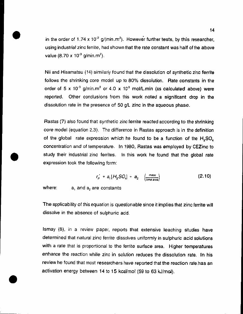
14

in the order of 1.74 x 10.2 g/(min.m2). Howevèr further tests, by this researcher,

using industrial zinc ferrite, had shown that the rate constant was half of the above

value (8.70 x 10.3 g/min.m2).

Nii and Hisamatsu (14) similarly found that the dissolution of synthetic zinc ferrite

follows the shrinking core model up to 80% dissolution. Rate constants in the

order of 5 x 10.3 g/min.m2 or 4.0 x 10.3 mol/L.min (as calculated above) were

reported. Other conclusions from this work noted a significant drop in the

dissolution rate in the presence of 50 g/L zinc in the aqueous phase.

Rastas (7) also found that synthetic zinc ferrite reacted according to the shrinking

core model (equation 2.3). The difference in Rastas approach is in the definition

of the global rate expression which he found to be a function of the H2S04

concentration and of temperature. In 1980, Rastas was employed by CEZinc to

study their industrial zinc ferrites. In this work he found that the global rate

expression took the following form:

( mass )

Irmearea (2.10)

where: a, and a2 are constants

The applicability of this equation is questionable since it implies that zinc ferrite will

dissolve in the absence of sulphu ric acid.

Ismay (8), in a review paper, reports that extensive leaching studies have

determined that natural zinc ferrite dissolves uniformly in sulphuric acid solutions

with a rate that is proportional to the ferrite surface area. Higher temperatures

enhance the reaction while zinc in solution reduces the dissolution rate. In his

review he found that most researchers have reported that the reaction rate has an

activation energy between 14 to 15 kcal/mol (59 to 63 kJ/mol) .

•

•

•

15

Filippou (9) recently studied the leaching kinetics of industrial zinc ferrite (provided

by CEZinc) and found the dissolution process was best represented using the

"grain model" whose characteristlc equation is given by:

(2.11)

where: 8g and Vg : grain surface area and volume respectively

F g: shape factor (for spherical grains Fg=3)

With a shape factor of 3, the "grain" model is similar to the characteristic

"shrinking core model" (equation 2.3). His results agree with those of Eigersma

and Rastas in that the surface reaction, and not diffusion, was found to be the rate

controlling step. This is not surprising since the zinc sulphate product dissolves

in the fluid .

Filippou also proposed that the following equation described the kinetics for the

dissolution of industrial zinc ferrite in the presence of a H2S04-ZnS04-Fe2(SO~b

system:

054 r = k aH' (

mol ) lime' volume

with k dependent on temperature according to the Arrhenius expression:

k = 3.8xI0' exp ( -64.8R~JlmO/J

(2.12)

(2.13)

Equation (2.12) takes a similar form to equation (2.6) with the exception that the

H+ activity has a 0.54 order dependency on the rate instead of 0.50, and the Fe3+

activity does not appear in the equation. At 98°C (371.15 K), which was the

operating tempe rature of the jarosite pilot circuit, the rate constant for the above

kinetic expression is equal to: k (98°C) = 2.88 x 1 0'6 (mol~46. L 0 54 / m2.min)

•

•

•

16

Filippou's calculated activation energy of 64.8 kJ/mol (15.5 kcal/mol) lies close to

the range which was reported by Ismay. In equation 2.12, the activity of hydrogen

is employed. This feature allows this rate expression to account for the negative

effects that high zinc and iron concentrat:ons in solution have on the dissolution

rate. It was postulated that the plesence of other electrolytes would result in a

decrease in the activity of the hydrQgen ion. The ha If order dependency on the

hydrogen ion activity was calculated by plotting the log of the derivative of the

conversion with time (dx/dt) against the log of the acid concentration. This method

results in a straight line with a slope equal to the order of the reaction. This

method is acceptable if it is valid to assume that the partie le surface area is

constant for a given conversion. It was also found, as expected, that temperature

resulted in an increased dissolution rate but that agitation speed had no significant

effect. These results confirm that the reaction is not diffusion controlled since mass

transfer is not affecting the rate .

2.3 Jarosite Precipitation Kinetics

Jarosite precipitation is a nucleation reaction in which the reagents react to form

jarosite nuclei and then these nuclei subsequently grow to produce Jarosite

crystals. For ammonium jarosite precipitation the reaction is as follows:

3Fe 3 + + NH4' + 2S0t + 6H2 0(aq) -7 NH4[Fe3(S04M0H)6](s) t 6H+(1.2)

Following the literature survey, it was found that there is a general agreement

amongst the various researchers as to the effects of the main variables on Jarosite

precipitation. This section will begin by discussing the parameters which effect

Jarosite precipitation. Following this review, various jarosite kinetic expressions

found in the literature will be outlined.

Induction Period and Jarosite Seeding Effects

An induction period was first observed by Steintveit (10) and was found ta

disappear through the addition of jarosite seeds. Ismay (8) reports that since

•

•

•

17

jarosite precipitatirln involves hydrolysis and crystallization, this induction period is

due to the slow formation of a sufficient number of nuclei. Although jarosite

seeding does not change the final equilibrium iron concentration, it does drastically

shorten the time required for jarosite precipitation (11).

Qian-kun (1 2) found that jarosite seeding increased the jarosite precipitation rate

and thus the rate of iron removal from solution. Through the addition of 25 ta 190

g/L seed the time required for precipitation in their tests was reduced by several

hours (over 75 %).

Limpo (13) reports that the rate is dependent on the surface area of seed crystals

and that since the velocity of growth of jarosite cryslals is greater than the rate of

nucleation he concludes that the number of nuclei controls the rate of

precipitation, which is in agreement with Ismay .

Effect of Reactant and Product Concentrations

The jarosite precipitation reaction stoichiometry, given by Equation 1.2, shows that

ferric iron, and ammonium in solution are reactants and acid is a product. The

literature review confirms that increased concentration of these reactants increases

the jarosite precipitation kinetics. Similarly the rate of precipitation is reduced

when high concentrations of acid are present. For example, several researchers

(1,8,12) found that higher than stoichiometric proportions of alkali (ammonium ion)

increased the rate of jarosite precipitation.

It was found (12,13) that although high initial ferric iron concentrations would

increase the rate of Jarosite precipitation, the final iron concentration was always

higher than the case where lower initial concentrations were examined. An

expression for Jarosite precipitation developed by Rastas (7) showed that the rate

of iron precipitation depended strongly on the ferric sulphate"Concentration. This

expression will be shown in the next section.

•

•

•

18

Since acid is produced du ring jarosite precipitàtion, a high acidity was found to

reduce the amount of iron removal (this fol/ows the reaction stoichiometry). It is

apparent that although high initial acid concentrations are found to increase zinc

ferrite leaching, a compromise is necessary for the optimum operation of the

jarosite conversion circuit.

Effect of Temperature

Limpo (13) found that the reaction rate increased by a factor of three wh en the

temperature was increased from 90 to 100 oC. Qian-kun and co-workers (12) also

found that the iron removal rate was enhanced when tempe rature was increased

from 85 to 98 oC. Final/y, Kubu et al. (15), confirmed that increasing the

temperature would invariably promote jarosite precipitation.

Hydronium Ion Substitution:

The precipitation of al kali jarosite has an additional complication which arises from

the co-precipitation of hydronium jarosite which tends to substitute itself for the

alkali portion of the jarosite compound. This was shown (11,12) through the non­

stoichiometric composition of the jarosite solids (the content of the alkali species

was deficient). The result is an alkali jarosite with the form:

{H30,NH4}[Fe3(S04)2(OH)6]' Further test-work (12) indicated that as temperature

increased from 80 to 100 oC hydronium ion substitution also increased. Above

100°C, however, the rate of hydronium substitution goes in the opposite direction.

Since the CEZinc conversion circuit is operating at 98 oC, both ammonium jarosite

(equation 1.2) and hydronium jarosite precipitation (equation 2.14) had to be

studied in order to take into account the ove rail rate of iron precipitation.

3Fe 3' + 7 H20(aq) + 2S0; --? H30[Fe3(S04)2(OH)6](s) + 5H+ (2.14)

•

•

•

19

Jarosite Precipitation Rate Expressions

Qian-kun (12) proposed the following expression for iron precipitation as

ammonium jarosite:

(2.15)

k, = 4.733x10" exp( -18.76~~Cal/mO/] (2.16)

k = 14.39 exp( -3.975 kCal/mO/] -1 RT

(2.17)

Once again, at the operating temperature of the pilot circuit (98°C) the rate

constants are as follows: k, = 42.41 and k. 1 = 6.57 x 10-2• Unfortunately no

units were provided in their paper. In this work, there is no mention of the

experimental apparatus used to obtain these kinetic data; consequently it is

assumed that the set-up was probably a constant volume batch reactor in which

they tried to limit the effects of external mass transfer resistances.

The thesis by Eigersma (14) has shown that the rate of jarosite production, r+ is

proportional to the linear crystal growth rate, G (mIs) and the surface area of tl-Je

jarosite crystal, A. The following equation describes this relationship:

(2.18)

Rastas (7) in his work on ferrite and jarosite kinetics found the following expression

to hold for the rate of iron precipitation as jarosite:

(2.19)

where the species concentrations are in g/L and the reaction orders with respect

•

•

•

20

ta each species ranged as follows:

a ::: 1.9 to 2.4 P == -3.5 ta -2.2

y::: 0.5 to 0.7 ô::: 0.8 ta 1.4

Rastas, when working with industrial CEZinc Jarasite in 1980, found the rate of

iran removal could be mode lied using the following constants for (x, ~, 'Y, and ô:

The rate constant at 98°C for the above expression was calculated by Rastas to

be:

k = 9.944x10 1 (g/L).0 56Bh(1 or 1.657x10>2 (g/L)O s6s.min>'.

It is important to note that equations 2.15 and 2.18 are not rate laws but are

design equations for a constant volume batch reactor. A rate law should not

depend on the reaction vessel, but on the local state of the system in terms of

temperature, pressure and composition, therefore, it should not have a differential

term in it. Another peculiarity in Rastas rate expression, is that he incorporates the

jarosite seed concentration into the equation. This term refers to the mass of dry

jarosite seed per volume of slurry. If we choose to assume that the jarosite seed

concentration is relatively constant, th en we could ignore this term by accounting

for it in the rate constant. For example, in most of the pilot experiments the

jarosite seed concentration was 150 g/L giving an overall rate constant, k' = 5.22x10>2 (g/L) l 2s3.min>1 .

•

•

•

21

Chapter'3 EXPERIMENTAL METHODS

3. 1 Overview

A total of four jarosite pilot plant process identification experiments were

successfully completed. In each of these experiments, the process was operated

under "normal" flow conditions (Table 111-1) for 12 hours. Following this initial

steady-state period, the flow-rate of one of the feed streams was increased by a

step change and the process response was recorded by taking successive

samples from the effluent streams of each of the five reactors. After seven hours

of operating under "step change" conditions, the adjusted feed stream flow was

returned to its original value, and the process response was once again recorded.

The tirne required for running an experiment consisted of two full days of

preparation, 24 hours of experimentation, and four days of: clean-up, sam pie

preparation and acid titrations. Approximately 300 samples were taken for each

experiment (150 each of solids and solutions). Each sam pie was subsequently

assayed for iront zinc, lead, copper, and lithium representing a total of 1500

determinations and 150 acid titrations per experiment. The cast of each

experiment was estimated at $9500. This amount covered the cost for analysis

of ail of the samples as weil as the price for the chemicals used in each run.

Since the pilot plant required more expensive construction materials due to the

corrosive nature of the process, approximately $10 000 of equipment was

purchased.

3.2 Pilot Equipment

Originally, it was proposed to carry out the process identification experiments on

the actual conversion circuit at CEZinc. This approach was abandoned since the

possibility of upsetting the leach circuit performance by exec.uting IIstep change"

tests was too great. It was further realized that a pilot unit allowed the flexibility

•

•

• ..

22

of operating under relatively steady and controlled transient conditions, which

would never have been the case if the actual circuit was employed due to the large

number of unmeasured process disturbances. In view of these benefits, it was

decided to construct a pilot scale set-up to resemble the first five tanks of the

conversion circuit at CEZinc. Photographs of the pilot equipment are displayed in

Figures 3-1 and 3-2 and a schematic of this circuit is shown in Figure 3-3 .

Actual Jarosite Pilot Circuit

The pilot reactors consisted of 5 continuo us stirred tanks in series. The tanks

were maintained at a constant temperature of 9aoe by the use of external heating

jackets. Since the actual process employs live steam injection to maintain the

reactor temperatures at 98°e, water was added to ail five tanks for the purpose of

•

•

•

23

simulating the dilution effect of the steam .

"

Figure 3·2 Actual Jarosite Pilot Circuit: View of First Tank

Zinc ferrite and jarosite seed slurries were independently pumped to the first tank.

ln the industrial scale operation at CEZinc, the jarosite seed mixes with the zinc

ferrite slurry before it enters the first tank. Since the ratio of zinc ferrite to jarosite

continuously varies at the plant, it was decided to have two separate slurry

streams entering the first tank so that the effect of varying the jarosite seed flow

could be examined.

Two acid streams, spent and raw, were also pumped to the tirst reactor. Both of

•

•

•

24

these acid stream flows were monitored using totameters (calibration curves are

shown in Appendix Il). The spent acid stream flow was substantially larger than

that of the raw acid stream (Table 111-1). The raw acid stream's sulphuric acid

concentration, however, was approximately 10 times larger than that in the spent

acid stream.

I ..... ,., ... ,..,J,.,.~ 1 .... ItO~J 'e. >-E;r--

I$~CN' Aè l o~ Il I ... "w ,,( JI) >-E:.J Il Il ~ ~ ~ ~ ."-~ ..... ATe ... r

-WW W W w rn rn n ij ! .~

rn ."-~ NH .. O ... I

.....

~ ..... - .. ~ ... -_ ... -_ ....

1 T"NKU

, ...

m .......

u ...... . .

'ANK "-

'IINK :J ~ ---- ... .. .. --- ..

TIINK "

TAN~U~

Figure 3·3 Pilot Scale Jarosite Circuit

TABLE 111-1

FEED STREAM FLOWS

1 FEED STREAMS 1 FLOW {mL/min} 1

Zn Ferrite Siurry 14.0

Jarosite Siurry 12.1

Spent Acid 16.1

Raw ACld 0.96

Ammonium Hydroxlde 2.2

Water 2.5

•

•

•

25

Ammonia was added to the third reactor, as ammonium hydroxide, as shown in

Figure 3-3, with the objective of increasing the rate of ammonium jarosite

precipitation. The flow-rate of lhis stream remained unchanged for ail four tests.

Ammonium is present in the two slurry streams and in the spent acid strearn. As

a result, the ammonium concentration in the first two tanks will normally range

from 3 to 4 g/L NH/. Since jarosite precipitation is known to become limited (5)

when the residual ammonium concentration is below 4 g/L in the circuit, the

majority of the ammonium jarosite is produced at the point of ammonium addition

(Le. tank 3).

REACTOR CONSTRUCTION

Figure 3-4 provides a closer look at the individu al tank construction. Ali of the tank

materials were constructed trom 316L Stainless steel. The tank height was 24 cm

with a 16 cm diameter. The tanks contained 4 baffles to enhance mixing, ariser

pipe near the over-flow exit to prevent short-circuiting of the reagents, and a drain

at the bottom for slurry removal after the experiment. The height of the over-tlow

exit was 17.5 cm which gave a reactor volume of approximately 3.5 L. The actual

operating volume was measUled at 2.8 L once agitation was introduced. Agitation

was accomplished by using an over-head mixer and a tour blade, 45° pitch

impeller having a length of 2.6 cm. It was postulated that the installation of the

riser pipe may result in sorne solid accumulation in the tank but this was not found

to be a problem during the jarosite experiments.

A residence time distribution test was carried out to evaJuate the mixing

characteristics of this tank design. The results from this test are provided in

Appendix III. In this study it was fOL!nd that these reactors, with the risers intact,

closely approximated an ideal continuous stirred-tank reactor (CSTR). It should

be noted that, instead of employing a riser pipe to reduce short circuiting of the

reagents, another method would have been to increase ij1e impeller speed .

Although this practice was not found to effect the rate of zinc ferrite leaching

•

•

•

26

Figure 3-4 Reactor Construction

according to the work by Filippou (9), it may significantly effect the rate of jarosite

precipitation by interfering with the crystal growth rate since the crystals may break

apart. Consequently the speed of each of the impellers was maintained at 700

rpm with the exception of the third tank which was maintained at 800 rpm.

INSTRUMENTATION

Figure 3-5 provides a scheméitic of the instrumentation used in the pilot plant. A

thermocouple located in each tank continuously measured the reactor temperature.

The tempe rature was maintained at the desired set-point by using tempe rature

controllers (TC) which automatically turned the power on and off to the heating

coils. The pH in each of the tanks was monitored and the impeller rpm was

•

•

•

27

periodically measured using a tachometer and' readjusted manually. The eight

solution flow-rates (spent acid. raw acid. ammonia and the five water streams)

were measured using rotameters and were essentially stable during the

experimentation period.

o . . , ,

1 ANK :.!

Figure 3-5: Pilot Plant Instrumentation

Self-calibrating penstaltic pumps were used to feed the slurries. In order to

measure the slurry flow using these pumps, the desired flow-rate was set and the

pump would adjust the shaft rotation in order to achieve this flow (based on water

and the tubing used). The actual slurry flow would then be measured using a stop

watch and graduated cylinder. The measured value would then be entered Into

the peristaltic pump controller and the pump would readjust its speed based on this

new data point. This procedure would normally have to be repeated two to three

times before the correct slurry flow was achieved. This typ~ of peristaltic pump

•

•

•

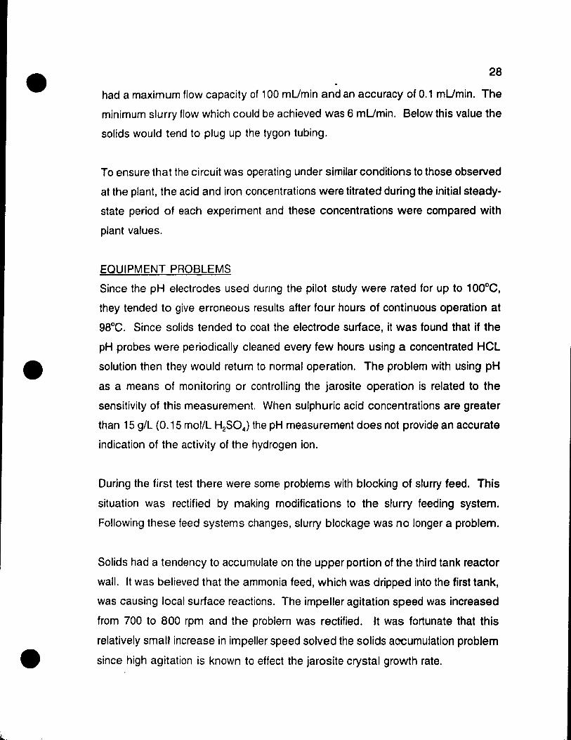
28

had a maximum flow capacity of 100 mUmin and an accuracy of 0.1 mUmin. The

minimum slurry flow which could be achieved was 6 mUmin. 8elow this value the

solids would tend to plug up the tygon tubing.

To ensure that the circuit was operating under similar conditions to those observed

at the plant, the acid and iron concentrations were titrated during the initial steady­

state period of each experiment and these concentrations were compared with

plant values.

EQUIPMENT PROBLEMS

Since the pH electrodes used dunng the pilot study were rated for up to 100DC,

they tended to give erroneous results after four hours of continuous operation at

g8De. Since solids tended to coat the electrode surface, it was found that if the

pH probes were periodically cleaned every few hours using a concentrated HCl

solution then they would return to normal operation. The problem with using pH

as a means of monitoring or controlling the jarosite operation is related to the

sensitivity ot this measurement. When sulphuric acid concentrations are greater

than 15 g/L (0.15 mol/L H2S04) the pH measurement does not provide an accurate

indication of the activity of the hydrogen ion.

During the tirst test there were some problems with blocking of slurry feed. This

situation was rectified by making modifications ta the slurry feeding system.

Following these feed systems changHs, slurry blockage was no longer a problem.

Solids had a tendency ta accumulate on the upper portion of the third tank reactor

wall. Il was believed that the ammonia feed, which was dripped into the first tank,

was causing local surface reactions. The impeller agitation speed was increased

from 700 ta 800 rpm and the problem was rectified. It was fortunate that this

relatively small increase in impeller speed solved the solids accumulation problem

since high agitation is known to effect the jarosite crystal growth rate.

•

•

•

29

3.3 Operating Procedure

FEEO STOCK OBTAINED FROM CEZinc

A volume of 500 litres of each of the following solutions was provided by the plant:

spent acid, low acid leach solution, and jarosite circuit solution. The zinc ferrite

slurry was prepared by mixing the low acid leach solution with the zinc ferrite

solids. Jarosite slurry fram the plant cou Id not be used directly in the pilot plant

experiments since the slurry was found to react during st orage as shown in the

Jarosite stability test which is summarized in Appendix IV. Consequently, jarosite

seed had to be prepared by filtering the plant's jarosite slurry from approximately

25% solids to 68% solids using a filter press. Since these filtered jarosite solids

remained essentially stable during storage, a batch of jarasite slurry was prepared

before each experiment. This was accomplished by mixing the filtered solids with

a measured amount of solution taken fram the CEZinc jarosite circuit thickener

over-flow stream .

FEEO STREAM PREPARATION

The spent acid solution obtained from the plant was used directly in the pilot set­

up. A 20 L batch of jarosite sluny was prepared for each experiment by combining

the 68% jarosite solids with enough jarosite circuit solution to praduce a slurry

which contained 33% solids. The zinc ferrite slurry was similarly prepared by

combining enough low acid leach solution with zinc ferrite solids to obtain a slurry

which contained 23% solids. Batches of zinc ferrite solids were produced at the

Noranda Technology Centre, by reacting 50 kg of calcine, which contains mainly

zinc oxide and zinc ferrites, with approximately 25 L of concentrated sulphuric acid

in a 250 L tank to produce approximately 15 kg of zinc ferrite solids. One batch

would provide enough solids for one experiment. Appendix IV outlines the

procedure for the preparation of the zinc ferrite sol Ids in more detai/.

Table 111-2 compares the composition of industrial zinc ferrite and jarosite solids

with their expected elemental compositions. The chemical formulae for zinc ferrite

•

•

•

30

and jarosite are ZnO.Fe20 4 and NH4[Fe3(S04MOH)6]' From this table we note that

the zinc ferrite composition is close to its elemental composition. The small

discrepancy is primarily a consequence of the industrial zinc ferrites containing

other species such as ferric hydroxide, lead sulphate, and other ferrites such as

magnesium ferrite, etc. The jarosite solids, obtained by filtering the plant's jarosite

slurry, are known to contain unleached zinc ferrites. Consequently, it is normal to

observe between 2.5 and 4.0% zinc in these solids. A more detailed examination

of the compounds present in these solids is shown in Appendix IV.

Table 111-2

COMPARISON OF INDUSTRIAL & ELEMENTAL SOLID COMPOSITIONS

SOUD EXPECTED ELEMENTAL (wt. %) INDUSTRIAL COMPOSITION (wt. %)

%Zn %Fe %Zn 'loFe

Zn FERRITE

1

27.1

1

46,3

Il

25,3

1

43.5

1 JAROSITE 0 349 2.9 33.0

The data in Table 111-3 show the average compositions and densities of the

aqueous phase of each of the feed streams. The raw and spent acid streams

contained the highest concentration of sulphuric acid but the lowest concentrations

of zinc and iron compared to the other feed streams. The zinc ferrite stream, on

the other hand, had the lowest acid and the highest zinc and iran concentrations.

Commercial sulphuric acid (96%) was used to simulate the plant's raw sulphuric

acid stream. Due to safety considerations, ammonium hydroxide (28% as NH3)

was pumped to the third tank instead of ammonia gas which is employed at

CEZinc .

•

•

•

31

Table 111-3

FEED SOLUTION COMPOSITIONS & DENSITIES

STREAM H2S04 Fe Zn LI Solution

NAME (g/L) (g/L) (g/L) (mg/L) Density

Zn FERRITE 2.0 9.1 957 2.54 1.30

JAROSITE 16.4 5.33 63.9 2.36 1 16

SPENT 188.2 7.0e·3 46.4 4.15 1.28

RAW ACID 1762.1 - - - 183

START-UP PROCEDURE

For the first test, a 17 L slurry was prepared for the purpose of filling each of the

5 tanks with an initial solution. This slurry contained a mixture of the following: 8.0

L of zinc ferrite slurry, 2.6 L of jarosite slurry, 6.1 L of spent acid, 0.3 L of water

and 68 mL of raw acid (Tank 1 only).

Following the first test, each of the reactor contents was reserved so that they

could be used as the starting solution for the subsequent test. With each of the

reactors full of the initial slurries, the band heaters were th en programmed to heat

the slurry to 70 oC. Once the pilot reactors reached this temperature, ail of the

feed stream flows were started as follows: five water inlets (which simulated live

steam addition at the plant), jarosite slurry & zinc ferrite slurry flows, spent & raw

acid flows, and the ammonium hydroxide flow. At this point the band heater set­

point was increased to the normal operating temperature of 98 oC

The circuit was then operated under "normal" conditions overnight for 12 hours

(refer to Table 111-1 for feed stream flows) to ensure that steady state was obtained

in ail five reactors. The following day, 3 to 4 samples trom each of the five tanks

•

•

• ...

32

were taken to quantify the initial steady state conditions. Once ail of the steady­

state samples were taken, a step change was induced in the circuit by changing

the flow of one of the feed streams.

The step change time was recorded and trequent sampling of the tirst tank was

initiated (approximately every 10 minutes for an hour). After 15 minutes, sampling

of the second tank began. Sampling of the third tank took place after 30 minutes

and so torth... After seven hours of operating under step change conditions, the

flow of the altered input stream was adjusted back to its initial conditions and the

time of this change was recorded.

Since this adjustment caused another transient state, the circuit is then sampled

as before. After seven hours of this second stage ot sampling, the band heaters

were turned off and each of the feed stream pumps were stopped. The tanks

were then emptied and inspected. The reactor slurries were reserved for

subsequent experiments and their volume and temperatures were recorded.

SAMPLING PROCEDURE

During Test:

Although it was realized that a large sample would be more representative of the

exit conditions, this practice would mean disturbing the exit stream flow, and

consequently the in let to the following reactor, for longer periods of time. Since

the exit flow was in the order of 40 to 50 mUmin it was decided to take a 50 ml

sam pie (approxil1iately) from the tank exit using a graduated cylinder (this took

approximately 1 minute). Before filtration, the slurry density was calculated by

measuring the sample volume and weight. Initially the temperature of the slurry

sample was recorded at the time of the density measurement. The sample

temperature was found ta be quite constant with variations between 68 and 72 oC.

Consequently this measurement was omitted .

•

•

•

33

Once the slurry density was recorded, the sample was filtered using a Büchner

funnel. It was important to filter the slurry as quickly as possible since it continues

ta react in the sam pie cylinder. The flltrate was saved and the solids were washed

with approximately 50 ml of hot water in order to remove any flltrate which may

have adhered to the solid surface. A 10 ml aliquot was taken from the filtrate

sam pie for analysis by an inductively coupled plasma (I.C.P.) analytical instrument.

The remaining filtrate sample was then reserved for subsequent acid titrations.

Analytical Methods:

ln arder to stabilize the filtrate samples, 10 ml of 30% nitric acid was added to

each aliquot. Th€·se samples were th en sent for iron, Zinc, lead, copper and

lithium analysis by I.C.P. The remaining filtrate samples, which were not stabilized

with nitric acid, were subsequently titratated for acid using a standard sodium

carbonate method. This analytical procedure is summarized in Appendix V .

The washed solid samples were dried at 70 oC overnight. The solids were then

weighed using a balance accu rate up to 2 decimal places (normally the sample

size was in the order of 10 grams). The dried solids were th en crushed and sent

for iron, zinc, lead, and copper analysis by I.C.P. A few of the feed stream solid

samples were sent for sulphate analysis (gravimetric method) in arder to give an

indication of the compounds present in the solid feeds. Appendix IV provides an

outline of these compound determination calculations.

3.4 Errar Analysis

As will be shown in the subsequent chapter, the mass balances for zinc, iron, and

lead in Tank 1 were ail above 89% and below 112%. The fol/owing analysis

shows that these mass balance results are quite good when we take into account

the large number of errors which normally arise during pilot plant experimentation.

Although this analysis deals mainly with sources of random error, it also touches

upon systematic errors which may have occurred.

•

•

•

34

As previously described in Section 3.3. slurry samples were taken at the exit of

each tank and the following parameters were measured: slurry density, filtrate

density, and percent sol Ids. Once each sample was filtered, the solutions were

titrated for acid and then sent to be analyzed for iron, zinc and lithium using an

I.C.P. (Inductively Coupled Plasma) instrument. The I.C.P. was also used to

analyze the solids for iron, zinc, and lead.

The error analysis will begin by calculating the errors involved using the sodium

carbonate method for acid concentration determinations. Following these

calculations the errors in using the ICP instrument will be discussed. Finally the

errors involved when measuring the density and the percent solids in the slurry will

be covered. A discussion on the use of tie elements for eliminating large sources

of error will demonstrate why it was decided to use the raw data without any tie

element manipulations .

ERROR IN ACIO TITRATION METHOD

A standard sodium carbonate method was used to analyze the acid concentration

in the filtrate samples. A detailed description of this method is shown in Appendix

V. The prepared titrant used in this method is standardized using a known

concentration of HCL. The titrant multiplication factors were 1.683 for Tests B, C.

and 0 and was 2.011 for Test E determinations. A 50 ml burette with

graduations of 0.20 ml, was used for titrant addition. This measurement

consequently resulted in a "Ieast count" of 0.10 mL. With this information, the

resulting precision in this me!hod can be calculated as:

Tests B, C, D:

Test E:

0.10 * 1.683 = 0.17 g/l H2S04

0.10 * 2.011 = 0.20 g/l H2S04

Typically a titrant volume of 28 ml had to be added to the samples trom the tirst

tank for acid analysis. Using this value, we can calculate the percent deviation

•

•

•

35

from the average acid concentration to be:

[H2S041 = (28 ml ± 0.10 ml) * 1.683 = 47.12 ± 0.17 g/L (± 0.36 %)

ERRORS IN USING I.C.P. ANAL YSIS

An Inductively Coupled Plasma (I.C.P.) atomic emission spectroscopy instrument,

which employs a matrix matching technique, was used to determine the zinc, iron,

and lithium in solution and the zinc, iron, and lead in the solids. At the

concentrations of acid, zinc, and iron which were present in the jarosite circuit, the

standard deviations would normally range trom 1 to 2%. In order to obtain an

estimate of the analytical precision, duplicates of several samples were analyzed.

Equation 3.1 shows this calculation which is referred to here as the sample

standard deviation in (%).

where:

%Std. Deviation = J LX' +X xl00% N-1

N = number of samples

x = difference between sam pie value and sample mean

X = sam pie mean

(3.1 )

The accuracy of the I.C.P. method is determined by spiking a known concentration

into each sample and then calculating the percent recovery. The recovery is

defined as the difference between the spiked sam pie and the initial sample

concentration divided by the concentration of the spike. Ideally, the accuracy

would be close ta 100% and the sample standard deviation would be as low as

possible. Table 111-4 outline~ the errors found during I.C.P. analysis of these

samples. In this table, "aq." refers to the aqueous phase and "s" refers to the solid

phase analysis .

•

•

•

36

Table 111-4

ERROR IN 1. C.P. ANAL YSIS

ANALYTICAL ZINC IRON LEAD LITHIUM

ERROR aq. 5 aq. 5 aq. S aq. s.

% STD. DEVIATION 19 1.3 2.5 1.5 20 1.2 5.5 --STO (g/L or % sohds) 1.7 0.1 0.6 0.5 - 0.04 .2 ppm --

% ACCURACY 101 94 112 116 90 83 82 ..

As seen in the above table, the percent standard deviation in the aqueous phase

is higher th an the deviations in the solid phase. In order to obtain improved

component mass balance results, it was hoped that lead could be used as a tie

element for calculating the mass fraction of solids in the slurry and that lithium

could be used tl) calculate the filtrate density. Although the lead standard

deviations are reasonable, the lead recoveries are too low in the solid phase for

lead to be a good tie element. It was planned to use lithium as a tie element in

the aqueous phase since it remains inert under the jarosite conversion circuit

conditions. Unfortunately, the errors are too large in both standard deviation and

accuracy for this measurement ta be able to adequately calculate another

parameter.

DENSITY AND % SOLIDS MEASUREMENT

Since the density and solids could not be inferred through tie element calculations,

the following describes the errors involved in each of these measurements. When

several measurements are required for calculating a parameter, we can estimate

the overall uncertainty in the measurement by using the following equation:

(3.2)

•

•

•

where: El = measurement errer of parameter i

R = relationship between the measured parameters

XI = measured parameter

37

A 50 mL cylinder with 1 mL graduations, resulting in a "Ieast count" of +/- 0.5 ml,

was used to measure the slurry sam pie volume. The balance used to weigh both

the solids and the slurry had a precision of +/- 0.05 grams. The average slurry

volume was 34.7 ml and had an average weight of 47.81 grams. For the slurry

density the average uncertainty was calculated as:

Siurry Density = 1.378 :t 0.020 g/mL (:t 1.4%)

The filtrate density was calculated by first placing a 10 ml ± 0.01 mL, in a sample

jar which weighed 11.2 ± 0.3 g. The filtrate weight plus the sample jar had an

average weight of 24.4 ± 0.05. The filtrate density was then calculated by

subtracting the weight of the sample jar from the total weight and th en dividing by

the sample volume. The resulting uncertainty was:

Filtrate Density = 1.320 :t 0.033 g/mL (2.5%)

The average weight of the dry solids sample was 5.53 grams. The error in the %

solids measurement was subject to the precision of the balance for both the solids

and the slurry weight where: % Solids = {Solids (g) / Siurry (g)} *100

Percent Solids = 11.57 ± 0.11 % (0.9%)

Fixed errors arose, however, due to the excessive handling required for each of

the solid samples: filtering, washing, drying and weighing. During these steps,

solids losses were always a problem. For example if an average of 0.5 grams were

lost during these procedures the average percent solids wou Id drop from 11.57 %

to 10.52 % (1.03 % solids difference) .

•

•

•

38

FLOW RATE MEASUREMENT

Rotameters were used tù measure the flow of raw acid, spent acid and ammonium

hydroxide. The calibration curves are given in Appendix II. Due to the variable

ranges in these aqueous stream flows and densities, differant sized rotameters

were employed. The smallest rotameter was used for the ammonium hydroxide

flow and the largest was used for the spent flow. The table below gives the

stream name, the corresponding fluctuation normally encounter and the associated

errer in flow which it produced. Fortunately the largest variability resulted in the

ammonium hydroxide flow which does not effect the operation of the first two

reactors.

Table 111·5

ERROR IN FLOW MEASUREMENTS

FLUCTUATIONS

STREAMS SCALE FLOW FLOW

(points) (mUmin) (%)

Ammonium Hydroxlde +/·3 +/- 0.4 +/·17

Raw ACld +/·2 +/·0.06 +/- 6 r-'

Spent ACld +/. 1 +/- 1.1 +/·7

l The two slurry streams employed self-calibrating metering pumps which could

deliver flows with a precision of 0.1 mUmin. During the course of the experiment,

the flow would tend to drift by 0.2 mUmin or approximately 2% of the average

slurry flow rates .

•

•

•

39

Chapter 4 EXPERIMENTAL RESULTS

4.1 Parameters Investigated

Experiments were performed with the purpose of studying the transient process

response to various step changes in the main feed stream flows. Altr,~ugh data

were obtained for ail five reactors, for the scope of this thesis, only the ~ èsults from

the first tank were analyzed in detai!. Table IV-1 summarizes the feed streams

which were varied during each of the four process identification experiments. The

purpose of conducting these types of tests was to obtain a better understanding

of the process dynamics. By inducing step changes in the feed stream flows we

can quantify the effect of this variable on the process .

Table IV-1

STEP CHANGE FLOWS

B [ INPUT STREAM FLOW (mUmin)

1 INPUT STREAM VARIED % CHANGE

1

NORMAL 1

STEP CHANGE 1

B Raw Acid 0.96 1.44 50

C Jarosite Siurry 12.1 182 50

D Spent ACld 16.1 242 50

E Zn Ferrite Siurry 14.0 175 25

The following paragraphs provide a description of each of the tests shown in Table

IV-1. The first test, denoted as TEST A, does not appear in the above table.

This experiment involved using zinc ferrite solids trom the plant. It was soon

realized that these industrial zinc ferrites solids were actually a mixture of 40%

•

•

•

40

ferrite and 60% jarosite. If we had used these solids for the entire test program

then it would not have been possible to study the effect of changing the jarosite

slurry flow rate since the system was already saturated with jarosite seed.

Consequently, it was decided to use prepared zinc ferrite, which did not contain

any jarosite solids, for the subsequent four experiments (Tests B to E). Since the

data from TEST A could not be compared with the other four tests, it was not

included in the analysis.

TEST B - Raw Acid Step Change

A 50% step change in the raw acid flow was performed in order to study the effect

of increased acid concentration in the circuit. It was realized that step increases

in the raw acid flow would result in higher acid concentrations in the first tank and

consequently would increase the rate of zinc ferrite leaching. Since the raw acid

is a concentrated solution of 96% H2S04 , the increased flow would not have a

diluting effect on the other species in the liquid phase and would furthermore not

have a measurable effect on the residence time in the reactors (Le. the residence

time decreased by 1 % from 60 to 59 minutes as a result of this step change).

TEST C - Jaros/te Siurry Step Change

A step change in the jarosite solids concentration was affected by increasing the

jarosite slurry flow by 50% while maintaining the zinc ferrite slurry flow constant.

Although these test conditions would result in an increase in the jarosite seeding,

a 14% reduction in the residence time (Le. from 60 to 52 minutes) would also

occur. Furthermore, since the jarosite slurry stream filtrate contains lower

concentrations of acid, zinc, and iron compared with the steady-state reactor

concentrations, we would expect the concentrations of ail of the species in solution

to drop in the first reactor. Furthermore, the jarosite solids contain lower mass

fractions of zinc and iron compared to the steady-state solids composition in this

first tank. Consequently the mass fraction of zinc and iron. in the overall solid

phase should also drop.

•

•

•

41

TEST 0 - Spent Acid Step Change'

A 50% increase in the spent acid flow was periormed in order to study the effect

of an increased acid concentration ln the circuit while diluting the zinc and iron

concentrations. This step change would also result in an 18% reduction (Le. trom

60 to 48 minutes) in the residence time. Increased acid concentrations as weil as

reduced zinc and iron concentrations should result in an overall increase in the

rate of zinc ferrite conversion as descnbed by the kinetic expression given by

equation 2.7.

TEST E - Zinc Ferrite Slufry Step Change

The effect of a step change in the zinc ferrite flow was studied in order to evaluate

increased loading or production on the jarosite circuit. Only a 25% increase was

initiated in this test since a larger change would lie outside any plausible operating

scenario at the zinc plant. This step increase would result in an 8% reduction

(from 60 to 55 minutes) in the residence time ln the circuit and a subsequent

dilution in the concentration of ail of the species in solution.

ln order to simplify the modelling of the jarosite circuit, it was decided not to study

the effect of temperature. Although it is weil known that temperature has a large

impact on both zinc ferrite leaching and jarosite precipitation the temperature

remains fairly constant in the actual conversion circuit at CEZinc. With this in

mind, the temperature in the reactors was controlled at 98°C by thermocouples

connected to temperature controllers which would turn the power on and off to the

external band heaters. A second thermocouple monitored the tank temperature

and this data was recorded using a data acquisition system. The amount of water

added ta each of the five tanks was adjusted during the first trial test (TEST A) :n

order to obtain correct solution densities. Once the required water flows ta each

tank were determined, these flows were kept constant during subsequent

experiments .

•

•

•

42

4.2 Mass Balances for First Reactor

ln each of the four experiments, the reactors experienced five sets of conditions:

1. Initial Steady State:

2. Step-Up Transient:

Ali tests were started at the same Initiai condillons.

Alter Inillaling a step Increase ln one 01 the inlet stream flows, the reactors experienced

translent condilions

3. Step-Up Steady State: The reactor would reach a new steady state condition under the step change flow.

4. Step-Down Transient: When the altered flow was re·turned to its original value, the reactor was once aga in under

translent conditions.

5. Final Steady State: The reactor would attalO a final steady state condition under the step-down flows.

The grouping of the data for the evaluation of the steady state concentrations was

accomplished by examining the solution and solids species composition profiles,

and selecting a group of points for each of the above outlined states. Data from

Test C, shown in Figure 4-1 demonstrates this rather subjective procedure .

TEST C: Jaroslte Slurry Step Change TANK 1

" Zn ln SoUds 10r-----------------------------------------~

aa.pUp 8tapDown

........... :',. ............... '

......... ·0 ...... ~ ... ~ ....... 7f-

6~--~--~----~--~--~~~~--~----~--~ o 100 200 300 400 1500 eoo 700 800 800

TIME (min)

Figure 4-1 Grouping of Data into Process States

•

•

•

43

The time span for each of these groups was as follows:

Initial Steady State: 95 minutes (1.6 hours)

Step-Up Transient: 121 minutes (2.0 hours)

Step-Up 5teady State: 184 minutes (3.1 hours)

Step-Down Transient: 118 minutes (2.0 hours)

Final Steady State: 121 minutes (2.0 hours)

From the above information it can be disputed that perhaps one or two additional

data points should have been added or discarded from the transient stages. It

was found, however, that small adjustments to the number of points in each group

did not have a large effect on the steady-state mass balance and reaction extent

calculations.

Mass balances for the first reactor were calculated for the three steady state

conditions as described above. The streams ente ring and leaving the first tank are

displayed in Figure 4-2. As described in section 3.2, there are five feed streams

entering tank 1 and two streams (slurry and water evaporation) leaving this

reactor. Ali of the inlet flows and densities were measured. The exit stream

density (refer to section 3.3) was also measured and the exit evaporation rate was

determined by conducting an evaporation test using Jarosite filtrate. The results

fram this study are shawn in Appendix III. An attempt was made to measure the

exit flow fram each of the reactor over-flow streams by taking samples for exactly

one minute and recording the sample volume. The resulting calculated flows,

however, were found ta be erratic fram sam pie to sample. Observations of the exit

stream showed that the outlet flow was actua"y flowing in spurts and a longer

average sample would give more steady results than a one minute sample. Since

it was impossible ta disrupt the exit flow for su ch long periads of time, it was

decided to calculate the outlet flow by performing a mass balance around each

tank .

•

•

•

Zn Ferri te Siurry

Jarosite Siurry 2

o Spent Ac i d

Figure 4-2 Jarosite Tank 1

Raw Acid ~==============~4

JAR. !

Water F==============95

Evaporation C\ ~II ======~~

JAR.! EXit=0

Siurry

Tank 1 exit Flow:

where,

5

E PnOn-Ms 0

7 = _n=_l __ _

P7

volumetrie flow of stream n, mUmin

density of stream n, g/mL

Mn: Mass flow of stream n, g/min

44

(4.1)

ln arder to get an understanding of the amount of data eollected for eaeh

experiment, Appendix VIII shows the assay results for the first tank in Tests B, C,

o and E. Following each steady state "process condition"~ an average and a

sample standard deviation was computed. The percent standard deviation was

•

•

•

45

then calculated by dividing the deviation by thè average value.

Table IV-2 shows the measLJred average slurry densities and the calculated

average exit flows during each steady state obtained during Test B. The effluent

slurry flow from the first tank, shown in the last column, was calculated using

Equation 4.1. In thb experiment, since a 50% increase in the law acid flow did not

result in a large increase in the overall flow out of the reactor, we can see that

manipulation of this stream does not have a significant effect on the residence time

in the reactor.

Table IV-2

TEST B - TANK 1 EXIT FLOW

1 1

'"' RAW ACID EXIT STREAM SLURRY

STEADY STATE FLOW (mUmin) DENSITY (glmL) FLOW (mUmin)

INITIAL 0.96 1.42 40.3

STEP CHANGE 1.44 1.43 40.6

FINAL 1.04 1.43 40.1

Tables IV-3 and IV-4 show the acid consumption as weil as the elemental zinc

mass balances for the first tank in Test 8. In these tables ail of the stream data

were measured with the exception of the exit stream flow, which was calculated

using equation 4.1 and the filtrate flow, F, calculated using the following:

P,Q, (1-XSOltdS) F, =-----

P ',I/rate.

(4.2)

P"ltrate : flltrate density, g/mL

XSOlldS: mass fraction of solids in the slurry stream

46 • Table IV-3

TEST B - TANK 1: ACID CONSUMPTION

TANK 1: Initial Steady State

Stream Stream Flow Siurry Denslty Fil!. Denslty Soilds Flltrate H2S04

Name # (mUmln) (glmL) (g1mL) (%) (mUmln) (g1L)

Fernte Siurry 1 14.0 1.473 1.298 16.5 13.3 2.00

Jar Siurry 2 12.1 1.385 1.156 30.9 10.0 16.43

Spent 3 16.1 _. 1.279 .- -- 188.20

Raw ACld 4 0.96 -- 1.831 . - .. 1762.10 JAR.l Exit 7 40.3 1.419 1.355 11.7 37.3 48.84 OVERALL IN OUT CHANGE % Reacted

(g/mln) 4.70 1.82 -2.88 38.74

(moI/min) 47ge-2 1.86e-2 ·294e-2

TANK 1: Step Change Steady State

Stream Stream Flow Siurry Density Fil!. Density Solids Filtrate H2S04

Name # (mUmln) (g/mL) (g1mL) (%) (mUmin) (g1L)

• Fernte Siurry 1 14.0 1.473 1.298 16.5 13.3 2.00 Jar Siurry 2 12.1 1.385 1.156 30.9 10.0 16.43

Spent 3 16.1 .. 1.279 .. .. 188.20 Raw ACld 4 1.44 .. 1.831 .. .- 1762.10 JAR.l EXit 7 40.6 1.433 1.339 11.6 38.4 59.88 OVERALL IN OUT CHANGE % Reacted

(g/min) 555 2.30 ·3.25 41.41 (mol/min) 5.66e·2 2.34e·2 -3.31e-2

TANK 1: Final Steady State

Stream Stream Flow Siurry Density Fil!. Density Soilds Filtrate H2S04

Name # (mUmln) (g/mL) (g/mL) (%) (mUmin) (g1L)

Ferrite Siurry 1 14.0 1.473 1.298 10.5 13.3 2.00 Jar Siurry 2 12.1 1.385 1.156 30.9 10.0 16.43

Spent 3 16 1 .. 1.279 . - _ . 188.20

Raw ACld 4 104 .. 1.831 .. . . 1762.10 JAR.l EXit 7 40.1 1.433 1.327 12.5 37.9 51.75 OVERALL IN OUT CHANGE % Reacted

(g1mln) 4.84 1.96 -2.88 40.47 (mol/min) 4.94e-2 2.00e-2 -2.94e-2 -•

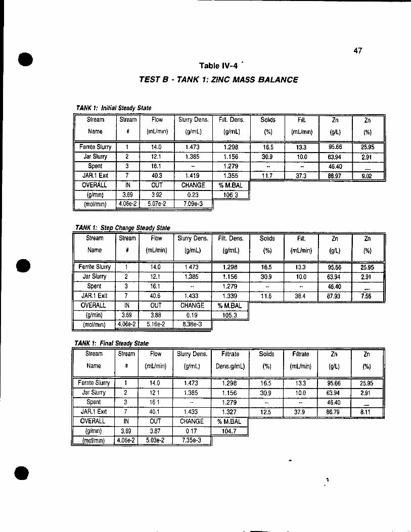
• 47

Table IV-4 •

TEST B - TANK 1: ZINC MASS BALANCE

TANK 1: Initial Steady State

Stream Stream Flow Siurry Dens. Fil!. Dens. Sohds Fil!. Zn Zn

Name # (mUmln) (g/ml) (g/ml) (Ofa) (mUmln) (g/L) (Ofa)

Ferrite Siurry 1 14.0 1.473 1.298 16.5 13.3 95.66 25.95

Jar Siurry 2 12.1 1.385 1.156 30.9 10.0 63.94 2.91 Spent 3 16.1 -- 1.279 .- -- 46.40 -

JAR.l EXit 7 40.3 1.419 1.355 11.7 37.3 88.97 9.02 OVERAll IN OUT CHANGE %M.BAL

(g/mln) 3.69 392 0.23 1063 (moi/min) 4.06e-2 5.07e-2 7.0ge-3

TANK 1: Step Change Steady State

Stream Stream Flow Siurry Dens. Fil!. Dens. Sohds Fil!. Zn Zn

Name # (mUmin) (g/ml) (g/ml) (%) (mUmin) (g/l) (%)

• Ferrite Siurry 1 14.0 1473 1.298 16.5 13.3 95.66 25.95

Jar Siurry 2 12.1 1.385 1.156 30.9 10.0 63.94 2.91

Spent 3 16.1 -- 1.279 -- -- 46.40 -JAR.l Exit 7 40.6 1.433 1.339 11.6 38.4 87.93 7.56

OVERAll IN OUT CHANGE %M.BAl (g/min) 3.69 3.88 0.19 105.3

(moi/min) 4.06e-2 5.16e-2 8.38e-3

TANK 1: Final Steady State

Stream Stream Flow Siurry Dens. Flltrate Sohds Flltrate Zn Zn

Name # (mUmin) (g/ml) Dens.g/mL) (%) (mUmin) (g/L) (%)

Ferrite Siurry 1 14.0 1.473 1.298 16.5 13.3 95.66 25.95

Jar Siurry 2 121 1.385 1.156 30.9 10.0 63.94 2.91 Spent 3 16 1 -- 1.279 -- -- 46.40 -

JAR.l EXit 7 40.1 1.433 1.327 12.5 37.9 86.79 8.11

OVERALl IN OUT CHANGE % M.BAL (g/mln) 3.69 3.87 017 104.7

(moI/min) 4.06e-2 5.03e-2 7.35e-3

•

•

•

•

48

The acid consumption and zinc mass balances are calculated by dividing the outlet

mass flow trom the reactor by the inlet flows. An example of this calculation is

given by equation 4.3.

(4.3)

where, Mn: Mass flow of stream n, g/min

sn : Mass fraction of solids in stream n, %

Sm : Mass fraction of component i in solids in stream n, %

Fn : Filtrate flow in stream n, mUmin

Cn.: Component i concentration in stream n, g/mL

The change in the number of moles of component is calculated fram;

(4.4)

where: Nn, is the molar concentration of component i in stream n (moi/mL). This

result will be used later to estimate the reaction extent.

ln order to correct for discrepancies in the mass balances, the change in the

number of moles for the zinc and iron was adjusted using the mass balance

closure result (which was normally close ta 100%) . This was accompli shed by

dividing the out let molar flow rate of element i by its calculated percent mass

balance result.

The percentage of acid consumed along with the solids that were leached in the

first reactor is shown in Table IV-5 for each of the four experiments. The average

initial acid consumption was approximately 37% for each of the tests. In each of

these experiments, however, the final acid concentration usuaJly differed trom that

observed during the initial steady-state condition due to problems in returning the

•

•

•

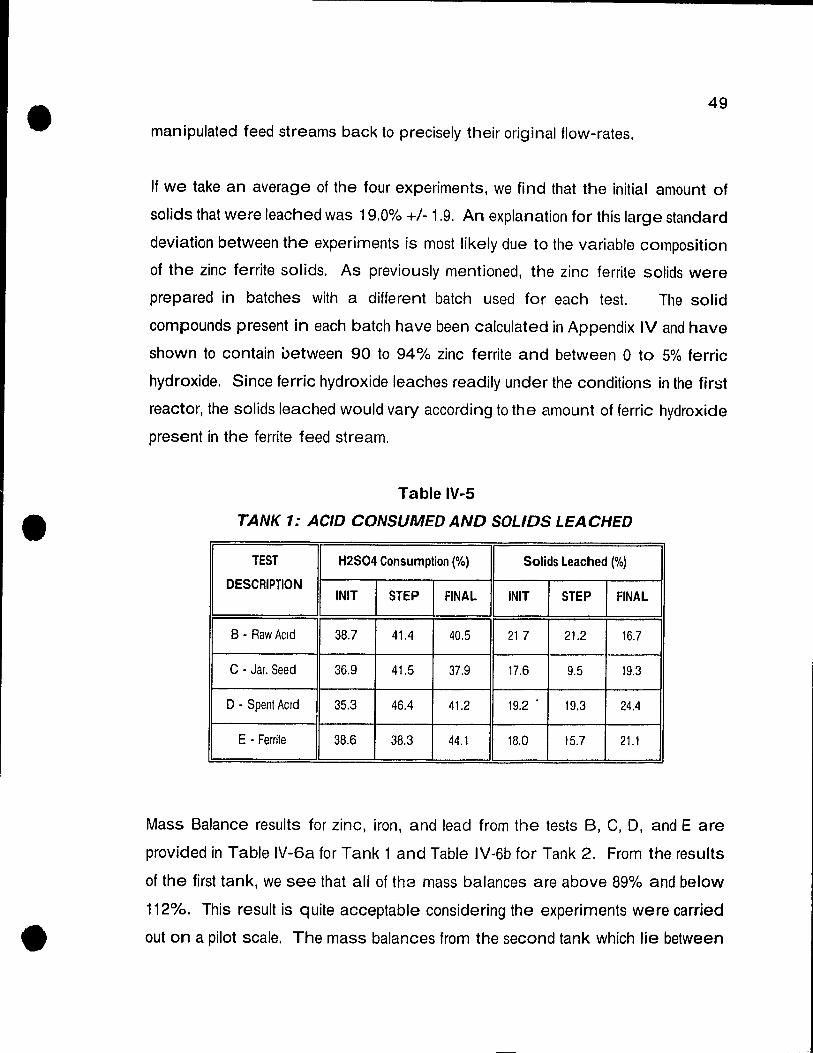
49

manipulated feed streams back to precisely their original flow-rates.

If we take an average of the four experiments, we find that the initial amount of

solids that were leached was 19.0% +/- 1.9. An explanation for this large standard

deviation between the experiments is most likely due to the variable composition

of the zinc ferrite solids. As previously mentioned, the zinc ferrite solids were

prepared in batches with a different batch used for each test. The solid

compounds present in each batch have been calculated in Appendix IV and have

shown to contain between 90 to 94% zinc ferrite and between 0 to 5% ferric

hydroxide. Since ferric hydroxide leaches readily under the conditions in the fin:;t

reactor, the solids leached would vary according to the amount of ferric hydroxide

present in the ferrite feed stream.

Table IV-5

TANK 1: ACID CONSUMED AND SOL/OS LEACHED

TEST H2S04 Consumption (0/0) Solids leached (%)

DESCRIPTION INIT STEP FINAL INIT STEP FINAL

B - Raw ACld 38.7 41.4 40.5 217 21.2 16.7

C - Jar. Seed 36.9 41.5 37.9 17.6 9.5 19.3

D - Spent ACld 35.3 46.4 41.2 19.2 . 19.3 24.4

E - Ferrite 38.6 38.3 44.1 18.0 15.7 21.1

Mass Balance results for zinc, iron, and lead fram the tests B, C, D, and E are

provided in Table IV-6a for Tank 1 and Table IV-6b for Tank 2. From the results

of the tirst tank, we see that ail of the mass balances are above 89% and below

1120/0. This result is quite acceptable considering the experiments were carried

out on a pilot scale. The mass balances from the second tank which lie between

•

•

•

50

88 to 130% are comparatively larger than the' results from the first tank. If we

compare the results from these two tables, it becomes clear that low mass

balances in the tirst reactor are tollowed by high mass balances in the second tank

since the errors are compounded.

Table IV-6a

TANK 1: MASS BALANCES FOR ZINC, IRON AND LEAD

TEST Zn MASS BALANCE (%) Fe MASS BALANCE (0/0) Pb MASS BALANCE (%)

DESCRIPTION INIT STEP FINAL INIT STEP FINAL INIT STEP FINAL

8 - Raw ACld 106 105 105 91 91 102 89 90 99

C - Jar. Seed 92 91 101 97 100 100 101 104 103

o -Spent ACld 93 98 94 100 112 100 98 103 95

E - Fe/rite 92 97 99 97 9B 91 96 101 97

Table IV-6b

TANK 2: MASS BALANCES FOR ZINC, IRON AND LEAD

TEST Zn MASS BALANCE (%) Fe MASS BALANCE (0/0) Pb MASS BALANCE ('10)

DESCRIPTION INIT STEP FINAL INIT STEP FINAL INIT STEP FINAL

B - Raw ACld 97 100 101 105 111 99 119 130 117

C - Jar. Seed 104 108 100 100 9B 100 111 110 117

o - Spent ACld 100 104 106 91 BB 95 110 115 116

E - Fernte 106 100 101 101 101 100 116 112 113

-~

•

•

•

51

4.3 Statistieal Analysis

To quantify whether a process change occurred during each of the step change

process identification experiments, a statistical examination of the steady-state

averages was conducted. A hypothesis test for the sample means was carried out

by using at-distribution with a 95% confidence limit. The details of this calculation

procedure are provided in Appendix VI. The hypothesis states that there is a

signifieant differenee between the sample means. Consequently, if the

hypothesis is accepted we can assume that a process change occurred. If,

however, the hypothesis is rejected, we can conclude that there is no significant

difference between the initial and the step change steady-state mean. The results

from this hypothesis testing are summarized in Tables IV-7a,b for the aqueous

concentrations and in Tables IV-8a,b for the solid species.

Table IV-7a

COMPARISON OF INITIAL & STEP CHANGE STEADY STATE

ACID CONCENTRATIONS FOR TANK 1

(0.2 g/L analytical error)

TEST AVG.INIT AVG. STEP INITIAL STD STEP STD Hest

DESCRIPTION [acid) (g/L) [acid] (glL) (glL) (glL) RESULT

8· Raw Acid 48.8 59.9 0.6 1.9 accept

C· Jar. Seed 46.5 46.9 0.1 0.4 reject

o . Spent ACld 43.8 62.8 2.5 3.0 accept

E· Femte 48.0 42.9 2.1 0.5 accept

As expected, the acid concentration was found ta increase during tests Band 0

where the flows of the strong acid streams were increased. The acid was found

to decrease during Test E due ta the dilution effect of the zinc ferrite slurry. In

Test C where the hypothesis was rejected, the acid concentration in the jarosite

•

•

•

52

slurry is approximately the same as the concentration found in the first tank; thus

no significant difference was expected.

Increased leaching of the zinc ferrites resulted in a rise in the iron concentration

after the step change in the Raw acid stream flow (Test B, Table IV-7b).

Increased ferrite leaching in Test D, however, was not enough to result in arise

in thfj iron concentration. This result. can be attributed to the dilution effect of the

spent acid stream as weil as the reduced residence time experienced in the first

reactor as a consequence ot this step change.

During the jarosite slurry step change test (Test C) a significant decrease in the

iron concentration was observed. This change may have resulted from either a

dilution effect since the jarosite filtrate has a lower iron concentration th an that

found in the tirst tank or from increased jarosite precipitation .

Table IV-7b

COMPARISON OF INITIAL & STEP CHANGE STEADY STATE

IRON CONCENTRATIONS FOR TANK 1

(0.5 - 0.9 g/L analytical error)

TEST AVG • .lNIT AVG.STEP INITIAL sro STEP STD T·TEST

DESCRIPTION [Fe] (glL) [Fe] (g1L) (g1L) (glL) RESULT

B· Raw ACld 249 27.6 0.9 0.8 accept

C· Jar. Seed 24 5 20.5 1.6 0.1 accept

o . Spent ACld 357 353 1 4 0.3 reject

E· Ferrite 236 24.4 0.9 0.8 reJect

•

•

•

53

Since the sam pie variance for the soluble zinc analysis was quite large, the

hypothesis was rejected for each of the four experiments. Consequently, no

conclusions can be drawn fram this data.

Table IV-Sa

COMPARISON OF INITIAL & STEP CHANGE STEADY STATE

IRON IN SOLIDS FOR TANK 1

(0.5 % solids analytical error)

TEST AVG.INIT AVG. STEP INITIAL STD STEP STO T-test

DESCRIPTION Fe(%) Fe% (%) (%) Result

B· Raw ACid 327 303 0.5 0.3 accepl

C· Jar. Seed 35.6 35.4 0.5 03 reJecl

D • Spent ACld 358 35.3 0.4 03 reJecl

E • Ferrite 354 338 0.1 o 1 accept

Although both tests 8 and D resulted in increased acid concentrations, which

should translate into increased zinc ferrite leaching, the iron in the solids was

found to drop significantly in Test B only (Table IV-Sa). Surprisingly, a significant

drop in the iron concentration occurreti in Test E where the zinc ferrite solids flow

was increased. Since the zinc ferrite solids contain more iron th an the tank 1

solids, this process change should have resulted in an increase in the percent iron.

The discrepancies in the above results can be attributed to the large (Le. 0.5 mass

fraction % ) analytical error involved in iron determinations .

•

•

•

Table IV-Sb

COMPAR/SON OF IN/TIAL & STEP CHANGE STEADY STA TE

ZINC IN SOL/OS FOR TANK 1

(0.1 % solids analytical error)

TEST AVG.INIT AVG. STEP INITIAL STe STEP STO T·TEST

DESCRIPTION Zn (%) Zn (%) (%) (%) RESULT

B· Raw ACld 9,0 7.6 0,2 0.3 accep!

C· Jar. Seed 9,0 7.3 0,1 0.03 accep!

o . Spen! ACld 9,2 84 0,0 0.2 accep!

E· Ferrite 8,6 103 0,1 0.2 accep!

54

The mass fraction of zinc in the solid phase (Table IV-Sb) decreased substantially

during the step change steady-state in tests Band D. This composition change

is due to increased zinc ferrite leaching resulting trom higher acid concentrations

in the first reactor following the step increase in the acid stream flows. The large

drop in the zinc composition in the solids observed during Test C was a

consequence of the increased jarosite slurry flow to the reac1.or. Since the

industrial jarosite solids contain only a small percentage of zinc this result was

expected.

ln ail of the above statistical results, with the exception of the iren assay in the

solids, the standard deviation within the steady state conditions is normally larger

th an the analytical error. This observation demonstrates that other errors resulted

from random variations in the feed stream flows and compositions as weil as from

sample handling.

It should be noted that in order to use the above hypothesis -test, it is necessary

•

•

55

to assume that the population variances between the sam pie sets ale essentially

the same. To verity this criterion, an F test was performed on the sample

variances. Results fram this calculation demonstrated that there were no

significant differences between the sample variances. This conclusion helps to

validate the use of the t-distribution hypothesis test.

4.4 Determination of the Rate Constant

For a constant volume eSTR with multiple reactions, the change in the molar

concentration of component i wlth time can be wntten as follows:

dC, dt

(FFfED - FEXIT ) LJ

= ' .... v r V JI J

ri

(4.5)

At steady-state, the change in the number of moles of i with time is equal to zero.

By combining the definition of the reaction extent;

J

F EX1T - FFEED == LV JI CJ , 'J"I

(4.6)

with

J

FEX1T - FFEED = LV JI rJ V , J-l

(4.7)

we can obtain the following:

(4.8)

There are two marn reactions occurring ln the conversion circUit. The first is the

dissolution of zinc ferrite, and the second is the precipitation of jaroslte. Using the

reaction rate expressions obtained from the literature review, we can calculate a

reaction rate constant. This result will then be used in the modelling work which

is covered in the subsequent chapter.

•

•

•

56

For the kinetics of zinc ferrite dissolution, a rate /aw of the form suggested by

E/gersma can be assumed:

(4.9)

For jarosite precipitation, equation 4.10 can be used:

(4.10)

Due to the high concentration of acid present in the first jarosite reactor, we expect

a very small amount of jarosite precipitation. With this assumption, the jarosite

reaction extent can be neg/ected and the extent of the tirst reaction can be

ca/cu/ated from the experimenta/ resu/ts:

(FFEED - Fn ) € = " 1

V, (4.11)

To ca/cu/ate the rate constant, k1, we can combine equations 4.8 and 4.9 to give:

k = E, 1 [Fe',! 1 VTAN1< ~ [H']

1

(4.12)

Tab/e IV-9 gives a summary of the reaction extents and the corresponding rate

constants ca/cu/ated using the average steady-state experimenta/ data for the

three components in solution. Within each experiment's steady state condition, the

reaction extent ca/cu/ated from 4.11 must be the same for ail components.

Furthermore, the rate constant k1 must be the same in ail cases. With this in

mind, an average rate constant was ca/cu/ated and found to be equal to:

1.76 x 10.3 +/- 0.28 (mol/L.min) .

•

•

•

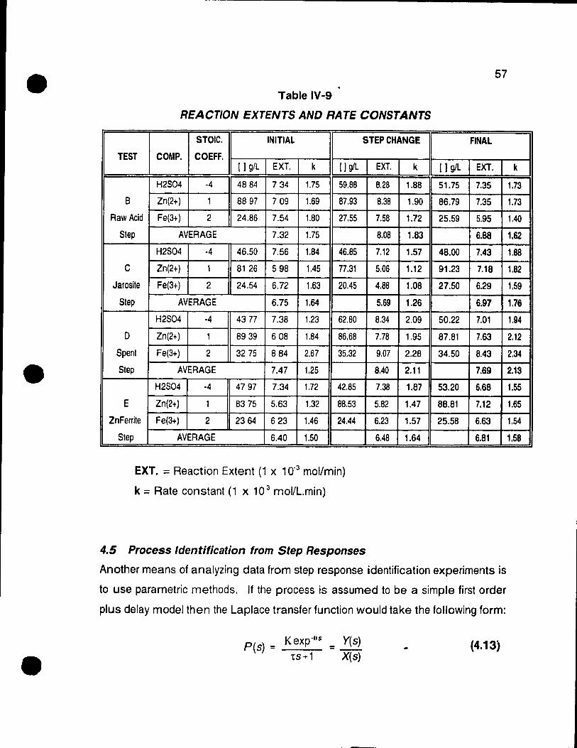
Table IV-9

REACTION EXTENTS AND RATE CONSTANTS

STOIC. INITIAL

TEST COMP. COEFF. ! 1 g/L EXT. k ! 1 glL

H2S04 ·4 4884 734 1.75 59.88

B Zn(2+) 1 8897 709 1.69 87.93

Raw Acid Fe(3+) 2 24.86 7.54 1.80 27.55

Step AVERAGE 7.32 1.75

H2S04 ·4 46.50 7.56 1.84 46.85

C Zn(2+) 1 81 26 598 1.45 77.31

Jarosite Fe(3+) 2 24.54 6.72 1.63 20.45

Step AVERAGE 6.75 1.64

H2S04 ·4 4377 7.38 1.23 62.80

0 Zn(2+) 1 8939 608 1.84 86.68

Spent Fe(3+) 2 3275 884 2.67 35.32

Step AVERAGE 7.47 1.25

H2S04 ·4 4797 7.34 1.72 42.85

E Zn(2+) 1 8375 5.63 1.32 88.53

Zn Ferrite Fe(3+) 2 2364 623 1.46 24.44

Step AVERAGE 6.40 1.50

EXT. = Reaction Extent (1 x 10.3 mol/min)

k = Rate constant (1 x 10 3 mol/Lmin)

STEPCHANGE

EXT. k

8.28 1.88

8.38 1.90

7.58 1.72

8.08 1.83

7.12 1.57

5.06 1.12

4.88 1.08

5.69 1.26

8.34 2.09

7.78 1.95

9.07 2.28

8.40 2.11

7.38 1.87

5.82 1,47

6.23 1.57

6.48 1.64

4.5 Process Identification from Step Responses

57

FINAL

[ 1 glL EXT.

51.75 7.35

86.79 7.35

25.59 5.95

6.88

48.00 7.43

91.23 7.18

27.50 6.29

6.97

50.22 7.01

87.81 7.63

34.50 8.43

7.69

53.20 6.68

88.81 7.12

25.58 6.63

6.81

Anather means of analyzing data fram step response identification experiments is

to use parametric methods. If the process is assumed to be a simple first order

plus delay model then the Laplace transfer function wauld take the follawing form:

K exp·os _ Y(s) P(s) = --

1s+1 X(s) (4.13)

k

1.73

1.73

1.40

1.62

1.88

1.82

1.59

1.76

1.94

2.12

2.34

2.13

1.55

1.65

1.54

1.58

•

•

58

where K is the process gain, 't is the dominant time constant of the process, and

e is the process de ad time. The terms Y(s) and X(s) refer to the Laplace

transforms of the output and input variables respectively. The estimation of the

process gain fram step response data is straightforward. The gain is defined as

the ratio of the magnitude of the output response to the change in the input step.

The process time constant is equal to the time it takes for the output response to

reach 63.2% of its final value (exp{ -1} = 0.632). The process dead time is the time

it takes after a step change is invoked until the output starts to respond. Figure

4-3 provides an illustration of this calculation procedure. The data used in this

graph are from Test 0 where the Spent acid flow was increased by 50%.

TEST D: Spent Acid Step Change TANK 1

[ H2S04 ] (g/L) 70 Step Up

85 ............. "- ...

80

55

50

45 ....

: 40

.. :..-.: . .

3!50 100

...... ....

1\Ip

200 300

Step Down ..

:~ Tdown

400 600 800 700 800 900

TIME (min)

Figure 4·3 Process Gain & Time Constant Estimation

Table IV-10 summarizes the process gains and time constants which were

calculated using data from the first tank. Since it was found that the first tank

responded immediately to ail of the step changes in the input stream flows, there

was no appreciable amount of process dead time.

•

•

•

59

Also included in this table are the estimated gains that would be observed in the

jarosite conversion circuit at CEZinc. These actual process gains were calculated

by using the observed pilot plant changes in compositions and relating these

values to the same percentage increase in the normal feed rate flows to the

industrial circuit.

Table IV-10

TANK 1: PRO CESS GAINS AND TIME CONSTANTS

STEP TEST

B

RAW ACID STEP

C

JAROSITE STEP

D

SPENT ACIO

E

Zn FERRITE

K pilot=

K plant=

COMPONENT K pilot (per mUmin) K plant' t pilot (min)

Up Down per m3/hr Up Down

H2S04 (g/L) 23.1 203 11 1 100 15

Fe (g/L) 56 4.9 27 100 -Zn(%) -30 -2.7 ·1 5 100 25

Fe (g/L) -07 -1 1 -0 3 60 90

Zn (%) -03 -0.3 -0.1 80 110

H2S04 (g/L) 2.0 1.6 0.8 50 35

Zn(%) -0.09 -0.04 -0.03 90 95

H2S04 (g/L) -1.5 ·2.8 -0 3 85 145

Zn (%) 05 06 01 50 75

• calculaled usmg "Up" respollse

g/L (or %Zn) change in concentration for each mL/min change

in flow

g/L change in concentration for each m3/hr change in flow

(used normal plant flows with same percentage increase as

pilot experiments)

t = process time constant (min)

From these results It is observed that the large st gains are found as a result of

changing the flow of the raw acid stream followed by changes in the spent acid

stream. Process hysteresis is apparent through the calculation of the process

•

•

•

-- ------------------------------------------------------

60

time constant. For example, the time constant for changes in the raw acid stream

flow is four times larger during the step up response. The opposite was observed

during the step changes in the slurry streams where the time constant during the

step down response was normally larger than during the step up transient.

Aesults trom a step change test ln the spent acid flow, conducted at CEZinc, gave

a process gain equal to 0.6 g/L [H2S04J per m3 spent. This result is comparable

to the estimated process gain from the pilot plant step change data which gave a

result of 0.8 g/L [H2S04J per m3 spent (Le. within 25%).

4.6 Discussion of Tank 1 Results

TEST B - Raw Acid Step Change

As expected, an increase in the raw acid stream flow resulted in increased zinc

ferrite leaching in the tirst reactor. This result was shown through the rise in the

acid and iron concentrations in the first reactor as weil as a drop in both the mass

fraction of iron and zinc in the solids.

This step change would also show an increase in the solution density and a

decrease in the slurry's solid mass fraction. After examination of the slurry and

solution densit.es, however, it is difficult to determine any definite trend that would

imply that the solution density was increasing or that the mass fraction of solids

in the slurry was decreasing.

TEST C - Jarosite Siurry Step Change

Increasing the Jarosite slurry f10w by 50% had the smallest impact on the

operation of the first reactor. The only change that was found to be statistically

significant was a reduction of the iron in solution by 4 g/L. Interestingly, this

reduction in iron is not only due to dilution effects since the drop would have been

in the order of 1 g/L. It is postulated that some additional jarosite precipitation

•

•

•

61

must have occurred. If this was the case, then it would explain why the acid

concentration did not drop by 2 g/L due to dilution since sulphuric acid is a product

of the jarosite precipitation reaction (reter to equation 1.2).

As expected, there was an obvious increase in the solids concentration in the

reactor effluent following the step increase in jarosite seed, however, no increase

in the slurry density was observed due to the lack of precision in this

measurement.

TEST D - Spent ACld Step Change

ln Test S, an addition al 0 85 g/min acid was introduced during the step change

while in Test D the increase in acid was almost twice this amount at 1.5 g/min.

The 17% reduction in residence time in the reactor, due to the increased spent

flow, atfected the amount of addition al zinc ferrite leaching. This result is apparent

when we compare results of Test D to those of B. For example, even though the

increase in acid was almost twice as large in Test D, the reduction of the percent

zinc in the solids, which gives an indication of the extent of zinc ferrite leaching,

was 0.8% compared to 1.4% in Test S.

TEST E - Zinc Ferrite Slurry Step Change

An increase in the zinc ferrite slurry flow simulates an increase in production.

Since zinc ferrite has a higher percentage of zinc and iran in the solids we are not

surprised to see the percent zinc increase in the first reactor after the step change

is introduced. As described in section 4.3, the iren did not respond as expected.

The discrepancy in the Iron composition in the solids was thought to be a

consequence of large variances in the analytical technique .

•

•

62 .

Chapter 5 DVNAMIC MODEl

5.1 Determlnistic Dynamic Model

The development of a deterministic dynamic model begins with writing the

appropriate transient mass, component and energy balances for the system. In

this study, since the reactor temperature was maintained essentially constant at

98°C, the energy was not considered.

It was desired to incorporate as many fundamental relationships into the model as

possible. It was realized that the utilization of available fundamental relationships

would result in a more robust model which would be able to predict, with sorne

degree of accuracy, the reactor performance under varying operating conditions.

Possible deterministic relationships may include known equilibrium, reaction

stoichiometry, kinetic and equipment geometry relations.

During the course of developing the jarosite circuit model, an experiment was

carried out to evaluate the mixing characteristics in the reactor (Appendix III).

From this test, we concluded that the reactors could be mode lied by assuming that

they behave as ideal stirred tank reactors. Consequently, the overall mass

balance for the reacting system is:

(5.1)

where: m and p are the number of feed and exit streams, respectively.

The component mass balance for the sa me system can be written as:

•

•

•

--- -------------------------------------------------------

63

(5.2)

where: k is the number of reactions occurring.

Since each of the reactor's main exit streams flow by gravit y, we can assume that

the tank volume remains constant. Also since the experiments showed that the

slurry and the filtrate densities were found ta vary in Tank 1 by less than 3%

during each process identification experiment, we can assume that they ramain

constant in the model. Using the above assumptions of constant tank volume and

constant density, equations 5.1 and 5.2, can be simplified as follcws (for the case

of one exit stream):

m

L P FEEDn OFEEDn - MEVAP (5.3) Q n"l

EXIT = ---------------PEXIT

and the component mass balances can be written as:

m

d(C) E (C,On)FEED - (C,Q)EXIT k ,EXIT n=l ~

= -----~---- + ~ v,J'J dt V J.1

(5.4)

If we assume a pseudo-homogeneous rate law (mass/L.min) for the

heterogeneous reactions, then we can write transient compone nt mass balances

for the solids as follows:

(5.5)

where: solid component concentration (m~ss/volume)

mass fraction of solid component i in the solid phase

•

•

•

-----.------------------------------------------------------------

64

mass fraction of solids in stream n

MI : molecular weight of solid component i

To simplify the jarosite model, only the main reactions which occur in the system

were considered. The first reaction, given by equation 5.6 below, represents the

dissolution of zinc ferrite. The subsequent two reactions are the precipitation of

ammonium jarosite and hydronium jarosite, respectively. Studies on jarosite

precipitation (11,12) have shown that when operating the jarosite conversion

process close to 1000e approximately 20% of the jarosite will be precipitated in the

hydronium form and the remainder will be as ammonium jarosite. These two

reactions are given by equations 5.7 and 5.8.

(5.7) 3Fe 3

' + NH4' + 2 sot + 6H20(aq) -7 NH4[Fe3(S04)2(OH)6](s) + 6H'

For modelling purposes, the two jarosite reactions are combined so that there is

80% ammonium and 20% hydroniurn jarosite formation. This combined jarosite

reaction is as follows:

15Fe3' + 4NH4' "' 10S0r + 31 H2 0(aq) ~

4NH4[Fe3(S04)2(OH)6](s) + HiJf.Fe3(S04)2(OH)6](s) + 29H' (5.9)

As shown in Appendix IV, during the batch preparation of the zinc ferrite solids,

ferric hydroxide may be formed. Since the percentage of ferric hydroxide was

sometimes found to be as high as 5% (as calculated in Appendix IV) the

dissolution reaction may be significant.

•

•

•

65

The ferrie hydroxide reaetion takes place as follows:

(5.10)

The following numbers were assigned to eaeh of the above reactions for reference:

Reaction 1 => r1 Zine Ferrite Dissolution

A + 8B c + 20 + 4E

Reaction 2 ~ r2 80% Ammonium & 20% Hydromum Jarosite Precipitation

150 + 4F + 1 QG + 31 E ~ 4H + 1 +

298

Reaction 3 => r3 Ferric Hydroxide Dissolution

J + 3B

where:

A = ZnO.Fe20 3 (8)

B = H+

C = Zn2+

o + 3E

o = Fe3+

E = H20

F = NH/

5.1.1 Incorporation of the Rate Equations

G = SO/" J = Fe(OH)3 (s)

H = NH4[Fe3(S04)2(OH)6] (5)

1 = H30[Fe3(S04h(OH)6] (5)

It has been shawn in the hterature that the rates of zinc ferrite dissolution and of

jarosite precipitation are controlled by their reaction kinetics. Ferric hydroxide

dissolution, however, is known to occur readily un der the highly acidic conditions

prevailing in the first jarosite reactor. Ta simplify the model, the ferric hydroxide

reaction is assumed ta occur instantaneously.

ln the literature review, there were two rate expressions given for zinc ferrite

•

•

•

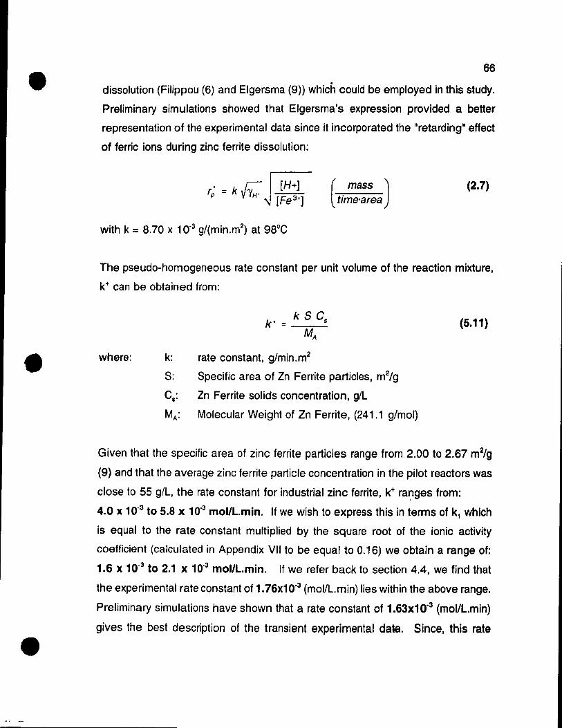
66

dissolution (Filippou (6) and Eigersma (9)) which cou Id be employed in this study.

Preliminary simulations showed that Eigersma's expression provided a better

representation of the experimental data since it incorporated the "retarding" effect

of ferric ions during zinc ferrite dissolution:

( mass )

time·area (2.7)

with k = 8.70 x 10.3 g/(min.m2) at 98°C

The pseudo-homogeneous rate constant per unit volume of the reaction mixture.

k+ can be obtained trom:

where: k:

S:

k+ = k S Cs MA

rate constant, g/min.m2

Specifie area of Zn Ferrite particles, m2/g

cs: Zn Ferrite solids concentration, g/L

MA: Molecular Weight of Zn Ferrite, (241.1 g/mol)

(5.11)

Given that the specifie area of zinc ferrite particles range from 2.00 to 2.67 m2/g

(9) and that the average zinc ferrite particle concentration in the pilot reactors was

close to 55 g/L, the rate constant for industrial zinc ferrite, k+ ra':1ges from:

4.0 x 10.3 to 5.8 x 10.3 mol/L.min. If we wish to express this in terms of k1 which

is equal to the rate constant multiplied by the square root of the ionic activity

coefficient (calculated in Appendix VII to be equal to 0.16) we obtain a range of:

1.6 x 10.3 to 2.1 x 10.3 mol/L.min. If we refer back to section 4.4, we find that

the experimental rate constant of 1.76x10·3 (mol/L.min) lies within the above range.

Preliminary simulations have shown that a rate constant of 1.63x10'3 (mol/L.min)

gives the best description of the transient experimental da~. Since, this rate

•

•

•

67

constant also falls within the range of the steady state experimental values given

in Table IV-9, it was used in the simulation of the first jarosite reactor.

Although two applicable jarosite precipitation kinetic expressions were found in the

literature it was decided to use the rate expression given by Rastas since the form

of the equation could be more readily used in this study. At 98°C the rate constant

was found by Rastas to be equal to 1.657x10·2 (g/L}0568 per min. Since equation

2.20 was actually written as the rate of iron removal and not as a rate expression,

the rate constant was corrected for the stoichiometry of reaction 5.9 as follows:

k* 1 ( J568

k = -15 MFe

(5.12)

This corrected rate constant is now used in equation 5.13:

(5.13)

5.1.2 TANK 1 Transient Madel

The transient mass balances for the first reactor were written using the stream

numbering shawn in figure 5-1. The flow rates of these feed streams are given in

Table 111-1. The raw acid stream was made up of 96% H2S04 (1760 g/L) and the

spent acid stream contained 180 g/L H2S04, 55 g/L zinc and several other species

at lower concentrations (Mn, Mg, NH/). Water was also added ta this tank ta

simulate live steam injection which occurs in the plant's jarosite circuit .

•

•

•

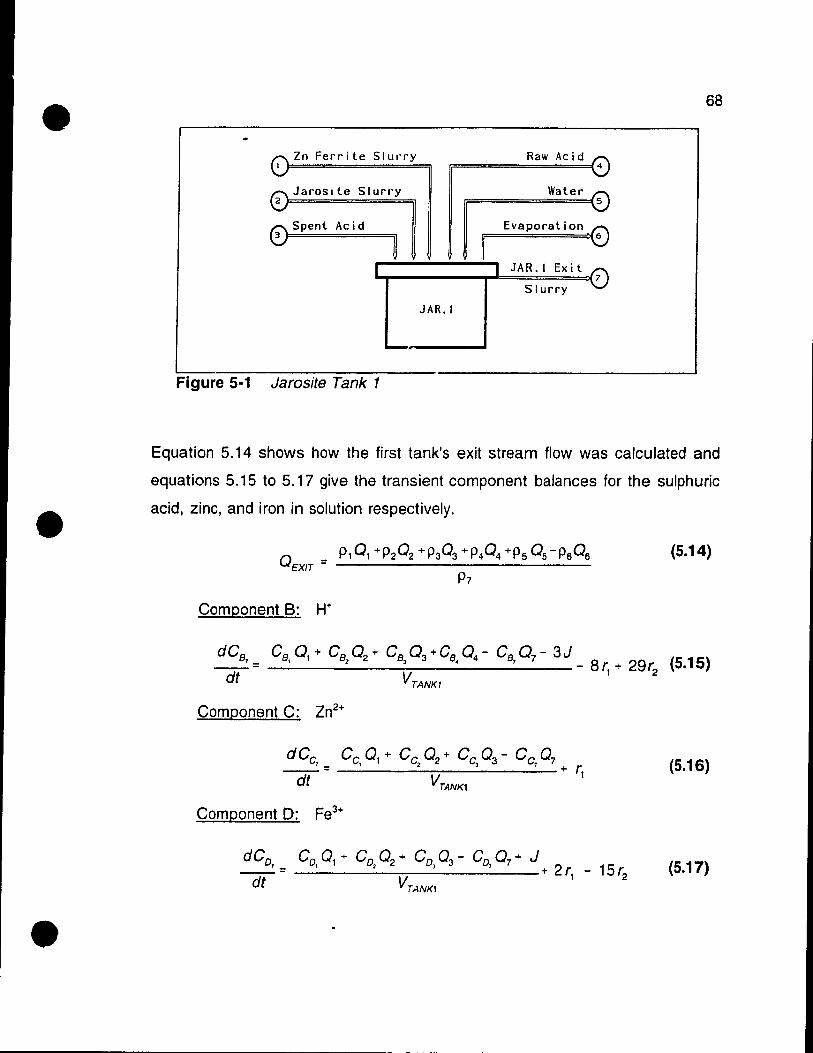
Zn Ferrite Siurry Raw Acid rr========(4

Water 2

Jaroslte Siurry rr=========(S

Evaporation 6

o Spent Acid

JAR.l Exit 0 ....,.------,,...=====~:- 7

Siurry

JAR.l

Figure 5·1 Jarosite Tank 1

68

Equation 5.14 shows how the tirst tank's exit stream flow was calculated and

equations 5.15 to 5.17 give the transient component balances for the sulphuric

acid, zinc, and iron in solution respectively .

(5.14)

Component B: H+

Component C: Zn2+

dCc 7 _

--- (5.16) dt

Component D: Fe3+

dCo 7 _

--- (5.17) dt

•

•

•

69

ln the abov~ equations, J refers to the molar flow rate of Fe(OH)3 entering the

reactor.

The mass fraction of zinc and iron in the solids were also modelled by writing

component mass balances (g/L.min) for the total solids, the jaroslte solids, and the

zinc ferrite solids concentrations as follows:

Component S: Solids

(5.18)

Component A:

(5.19)

Components H-I: Jarosite

(5.20)

The mass fraction of zinc in the solid phase was calculated uSlng the following

equation:

Cs %ZnA + Cs %ZnH_, %Zn Solids =., .~ x 100 %

Cs, (5.21 )

where, % Zn in specles i

The same procedure appli'"es for the calculatlon of the percent iron in the solids.

•

•

•

70

5.2 Proces$ Simulation Results

Following the reactor characterization test, tour "step change Il experiments were

carried out u~ing the pilot system with the purpose of validating the deterministic

model.

The transient component balance equations for sulphuric acid, zinc and iron in

solution and for zinc and iron ln the solids were programmed using the MATLAB

software package. T 0 solve these differential equations a 4th and 5th order Runge­

Kutta numerical integration technique was employed. In this study, the sensitivity

of the rate constants for zinc ferrite dissolution and jarosite precipitation were

explored.

ln the figures which follow, the vertical lines drawn on each graph represent the

step up and the step down times for each experiment.

TANK 1 RESULTS

For the first jarosite tank, it was found that the best model involved using the

previously calculated rate constants of kt=1.63x10·3 (mol/L.min) for zinc ferrite

leaching and k2=1.124x10·4 (mol/L)o 568 per min jarosite precipitation.

SULPHURIC ACIO CONCENTRA TlON PROFILES

Figures 5-2 to 5-4 demonstrate the changes observed in the sulphuric acid

concentrations for Tests S,D,and E respectively. The results trom Test C were not

included since the change in the sulphuric acid concentration was not found to be

statistically significant in this experiment (reter to section 4.3 where the t-test

hypothesis was rejected).

ln ail these figures, the model provides a reasonable representation of the changes

in the sulphuric acid concentration data .

• 71

TANK 1: Raw Acld Step Change

[ H2S04 ) (g/L) 70r----------------------------------------,

Step Up StepDown

400 100 200 300 400 fiOO 800 700 800 900

TIME (min)

k1 - 1.838-3. k2 - 1.1~

Figure 5-2 TEST B Sulphuric Acid Concentration Changes

• TANK 1: Spent Acld Step Change

[ H2S04] (g/L) 70~~~~------------~~=-=--------------, Step,Down

80

50 ...

Al. : 40

0 100 200 300 400 1500 600 700 800 900

TIME (min)

k1 - 1.es.a. 1c2-1.12~

Figure 5-3 TEST D Sulphuric Acid Concentration Changes

•

•

•

•

72

TANK 1: Zinc Ferrite Siurry $lep Change

[ H2804 ) (g/lJ 70r----------------------------------,

8lep Up Step Dow"

eo-

+

- • 400~~--~--~--~--~---~--~--~--~

100 200 300 400 aoo 800 700 800 800

nME (min)

k1 - UII3e-3. k2 - 1.12 .....

Figure 5·4 TEST E Sulphuric Acid Concentration Changes

FERRIC IRON CONCENTRATION PROFILES

The transient model provides a closer fit to the iron concentration data from Test

B, Figure 5-5, compared with that of Test C, Figure 5-6. One factor which

contributes to this difference is the standard deviation in the iron assay which is

around 0.6 g/L.

TANK1: Raw Acld Step Change

[ Fe8+ J (g/L) 32

a.pUp &tep DcIM'I 30 - .. 28 - ~ + 28' • .. • ~ : ... ... .. 2. r-" .. ;a."!it,.+ ;a. ...

• • 22 1-

20 1-

180 100 200 300 400 aoo eoo 700 800 800

nME (min)

k1 - 1 ....... Ica - 1.124e-4

Figure 5·5 TEST B Ferric Iron Concentration Changes

•

•

•

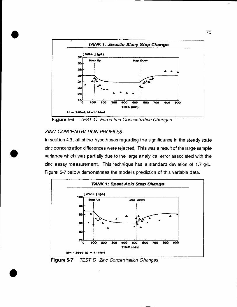
TANK 1: JaTOsite Siuny Step Change

[Fe3+ 1 (gIl.) 32r---------------------------------~

sa 28

--•

221-

201-

-.Up

. . ..

•••• 180~~~~~~--~--~~~--~--~--~

100 200 300 400 lIDO 000 700 000 800

TIME (min)

k1 - 1.a.a, 1d1-1.124e-4

Figure 5-6 TEST C Ferric Iron Concentration Changes

ZINC CONCENTRA TlON PROFILES

73

ln section 4.3, ail of the hypotheses regarding the sigmficance in the steady state

zinc concentration differences were rejected. This was a result of the large sample

variance which was partially due to the large analytical error associated with the

zinc assay measurement. This technique has a standard deviation of 1.7 g/L.

Figure 5-7 below demonstrates the model's prediction of this variable data.

TANK 1: Spent Acld Step Change

[Zn2+ 1 (gIl.) 100

s.pUp 8t.p Dawn

81

• :. • • t ~ • • • ~ • • .: •

80

7110 100 200 300 400 IlOO eau 700 800 800

T1M~ (min)

k1- 1.ea.a, Ica - 1.124e-4

Figure 5-7 TEST 0 Zinc Concentration Changes

•

•

•

74

ZINC MASS_FRACTION IN SOL/OS PROFILES

Sa me of the best representations of the experimental data are se en when we

compare the model's predictions with the percent zinc in the salids data. These

results are shawn in Figures 5-8 to 5-11 which look at Tests 8 ta E respectively.

TANK 1: Raw Acld Step Change

Zn Solld. <") 10~--.. ~-uP------------"---o.m----------~

1 .. '

~ .. 8-

7

.. 100 200

III - 1.a.a. lc2 - 1.1~

SOC) 400 soo nME (min)

..

eoo 700 800 800

Figure 5-8 TEST B Percent Zinc in Solids Changes

TANK 1: Jaroslte Siurry Step Change

Zn Solld. (") 10 8tIIp Up

.. .. .. .. ..

7

.. '0 100 200 SOC) 400 1500 800 700 800 80Q

nME (min)

lc1 - 1 ..... lc2 - 1.' ......

Figure 5-9 TEST C Percent Zinc in Solids Changes

As expected, the zinc mass fraction draps in Test Band 0 due ta increased zinc

•

•

•

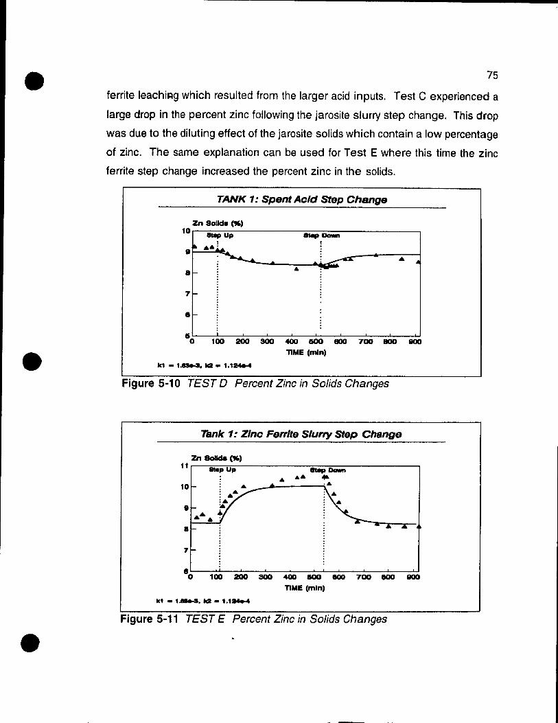
75

ferrite leachiRg which resulted from the larger acid inputs. Test C experienced a

large drop in the percent zinc following the jarosite slurry step change. This drop

was due to the diluting effect of the jarosite solids which contain a low percentage

of zinc. The same explanation can be used for Test E where this time the zinc

ferrite step change increased the percent zinc in the solids.

TANK 1: Spent Acld Step Change

Zn Solide <") 10 8t.ep Up

8

7

8

.. &tep Down

!

50 100 200 SOO 400 500 800 700 800 800

llME (min)

k1 - 1.a.3. lc2 - 1.124e-4

Figure 5-10 TEST 0 Percent Zinc in Solids Changes

Tank 1: Zinc Ferrite Slurry Step Change

Zn Solide <") 11~-.. =-p~u~p----------~&tep--~~------------~ ...... .. 10

8

7

80 100 200 300 400 500 800 700 800 800

llME (min)

k1 - 1.-..s. lc2 - 1.1~

Figure 5-11 TEST E Percent Zinc in Solids Changes

•

•

•

76

The modellin.9 results from the percent iron in the solids will not be discussed since

the data was found to be quite erratic. This can be partially explained by the

large analytical standard deviation of 0.5% Fe.

5.2.2 Tank 1 Jarosite Rate Constant Sensitivity

One of the questions that was studied was what was the degree of jarosite

precipitation in the tirst reactor knowing that the jarosite precipitation kinetics are

reduced under high acidities. Figure 5-12 shows the model results when the

jarosite precipitation reaction is ignored (ie. k2=O). From this Figure we see that

the two curves are essentially the same which implies that there is negligible

jarosite precipitation in the tirst reactor.

Tank 1: Zinc Ferrite Siurry Step Change

Zn Solld. (") 11~-=&~.p~U~P------------~&-.-P=D~--------------~ .. .. 10 . 4 ,,~, ':.:-' â,!.:."':"':":";:":":"""::":":':'':;

: .4.,' :. " :. g .

8

7

4 .. ~ •• Â ..

Jar. pptn. ride oonetant -1c2-1.1Z4e-4 '''112-0

1 00 200 300 400 500 800 700 800 800

T1ME (min)

k1 - l,ea.a

Figure 5·12 TEST E Effect of Jaroslte Precipitation

•

•

•

77

5.2.3 Tank:2 Results

ln the second tank the best results from the model were obtained when the zinc

ferrite rate constant was reduced from 1.63x10·3 to 0.85x10·3 (mol/L.min). This

was necessary since the rate constant for the first tank was originally calculated

with the assumption that the zinc ferrite solids concentration was 55 g/L. In the

second tank, the zinc ferrite solids concentration drops due to continued zinc ferrite

dissolution. Unfortunately, the experimental results cannot be used to calculate

the zinc territe solids concentration in the second reactor since jarosite precipitation

is occurring. As the best modelling results were realized for a rate constant of

O.85x1 0.3, we can propose that the zinc ferrite solids concentration may have been

reduced from 55 g/L to 29 g/L. The tact that the rate constant changes as a

function of the solids concentration demonstrates the limitations of modelling

heterogeneous reactions as pseudo-homogeneous reactions .

Since the rate constant that fitted the results trom the second tank was found to

be quite different from that of the first reactor, it was desired to study its sensitivity.

This was accomplished by comparing the following cases:

Case 1:

Case 2:

Case 3:

drop the zinc ferrite rate constant to 0.85x 10.3 and maintain

jarosite precipitation rate constant as in Tank 1

maintain zinc ferrite rate constant at 1.63x10·3 and maintain

jarosite precipitation rate constant as in Tank 1

maintain zinc ferrite rate constant at 1.63x1 0.3 and assume no

jarosite precipitation occurs (k2 = 0)

SULPHURIC AGIO CONCEN rRA TI ON PROFILES

If we refer to Figures 5-13 and 5-14 we find that the best modelling results occur

using the tirst case conditions in which the zinc ferrite rate constant is reduced by . 52%. Further examination of these figures shows that the worst results occurs

•

•

•

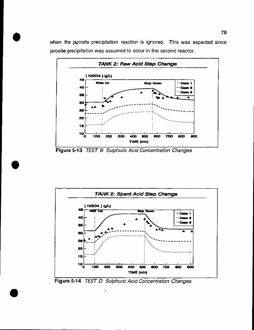
78

when the jarosite precipitation reaction is ignored. This was expected since

jarosite precipitation was assumed to occur in the second reactor.

TANK 2: Raw Acld Step Change

( H2S04 J (g/4 48~-----------------------------r----~

m.pUp

40

•

8tap Dawn -c..e1 .-c.... · .. c..ea

• • .. ~-_.---------~" 21!1 ".,- : ........... _------_.-;' ................. ~... --------

•••• "I -' '. '. "- --­ .............

10

0 100 200 300 400 500 eoo 700 800 IlOO

TIME (min)

Figure 5-13 TEST B Sulphuric Acid Concentration Changes

TAVK 2: Spent Acld Step Change

( H2S04 ] (g/~ 4S.-.unn.~----------~~~~-----r----~

-c...1 --c..e.

• "-c-a .. : .. -------------, : .", :' ~, ........................ ~ ... " ...

2& Â :,' ,0' : ", ... - .. ___________ _

---""'! ,: . ", , . . :,', .•..... . ...... . ........ , ........ .

••• -;a.:----""':.---f 30

20

18 .... I •• ~

1 0

0 100 200 SOO 400 1500 eoo 700 100 800

TIME (min)

Figure 5-14 TEST D Sulphuric Acid Concentration Changes

•

•

•

79

FERRIC IRON CONCENTRA TION PROFILES

For the case of the iron concentration, as seen in Figures 5-15 and 5-16, the most

important parameter seems to be the jarosite precipitation rate constant. If we

ignore this reaction, the model is no longer representative of the experimental data.

These Figures further demonstrate the negligible effect of the zinc ferrite rate

constant on the iron concentration profile.

TANK 2: Rl1w Acld Step Change

[ FII3+ J (g/L) ~'---~~p~u~p~----------ft8~~~~~----------~ 38 ...................... : .............. . 31 .........• ;........... . .....• 34; ~~ _______ ..

32 :

30

28

28

24

22

200

, . .. ,'~ ----~. .. :

-0..1

-'0.. a ,c-a

100 200 300 400 500 eoo 700 800 UOO

T1ME (min)

Figure 5-15 TEST B Ferric Iron Concentration Changes

TANK 2: Jaroslte Slurry Step Change ---------[ Fe3+ J (g/L)

~.---·--------------------------------ï 38 ~Up

38 ••......• . .•..••....•... S4 ;' •••• • ••••••

32

30

28

28 24 22

- .. " .................................................... ~ ...... """ . ... . . --.:...... : .-------: ~ ~~--: .M .c ....... __ : .4. .. ~ -0- 1 • •• - - - - - -... - - - - -.011 .. ; • • .;.& -'0-2

200 100 200 300 400 500 eoo 700 800 UOO

TlME (min)

Figure 5-16 TEST C Ferric Iron Concentration Changes

•

•

•

80

ZINC CONCENTRATION PROFILES

As expected, the zinc concentration is more sensitive to the adjustments in the

zinc ferrite rate constant since the zinc in solution is not affected by changes in the

rate of jarosite precipitation.

TANK 2: Spent Acid Step Change

[ Zn2+ ] (g/L) 105~--------------------------------~ 8tIIp Up &tep Down

100 ---0; .... .... , ..

90

86

.. .. .. .. ' ............

"- --- ......... ....... ~ ....

-Caae 1

--eue st . -Caae S

80~--~--~--~--~--~~--~~~--~ o 100 200 300 400 500 800 700 800 800

TlME (min)

Figure 5·17 TEST D Zinc Concentration Changes

ZINC MASS FRACTION IN SOL/OS PROFILES

TANK 2: Jarosite Siurry Step Change

Zn Solide (") 8'-~8tIIp~~Up~-----------'~~e~pR~=w=m~---------'

a

7

8

5

4

··· .. ····i·. . .

.. -.......

. ... . ..... .

----_ . ... ~---- ~~~#------ ----- -;.---... .,." ~-----; -Cue1 - -cu. st

"-cu. s 3~--~--~--~--~--~~~--~~----~ o 100 200 300 400 500 800 700 800 800

TIME (min)

Figure 5·18 TEST C Percent Zinc in Solids Changes

•

•

•

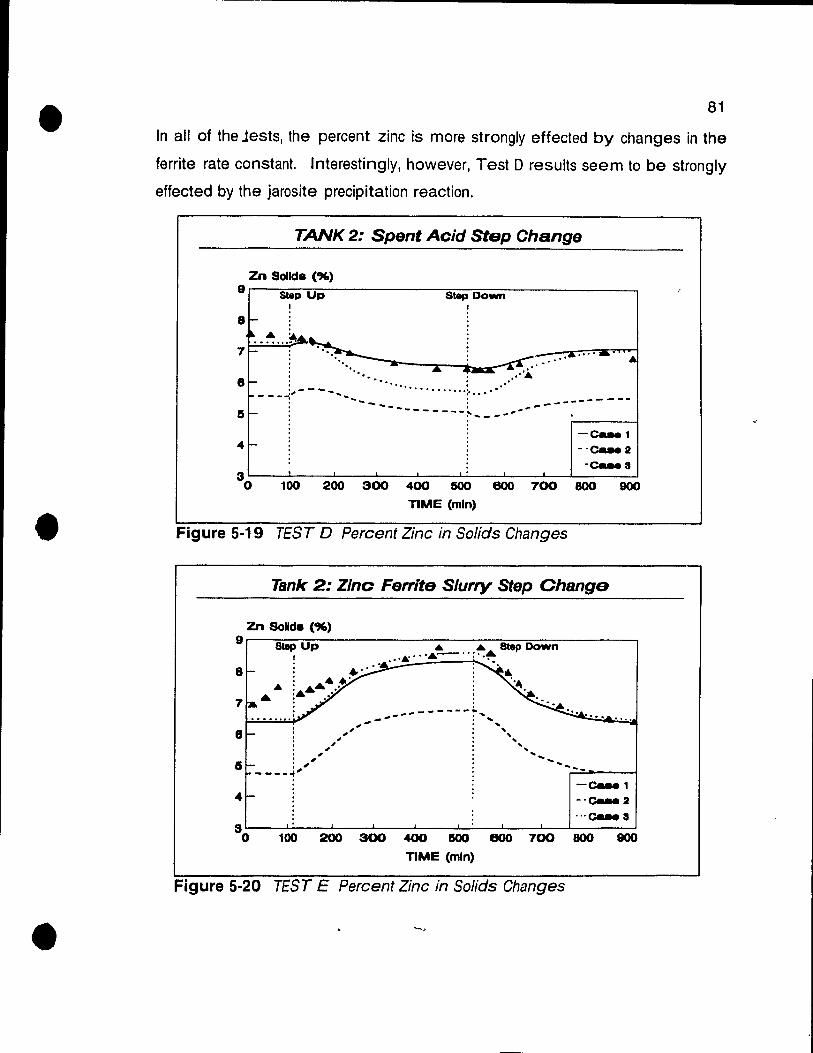
81

ln ail of the Jests, the percent zinc is more strongly effected by changes in the

ferrite rate constant. Interestingly, however, Test D results seem to be strongly

effected by the jarosite precipitation reactiono

TANK 2: Spent Acid Step Change

Zn Solide (%) 9'-~S~W~p7U~p------------~S~t~~Do~wn=-----------~

1

8

8 --­ .... .0'- ..

•• 0

.......... ; ..... -- -_"." -- --... .......... ------------- .. _------~--_ .. -.... -!5

-Caae1 4 -·ea..2

-ea.. 3

30 100 200 300 400 500 800 700 800 900

TIME (min)

Figure 5-19 TEST 0 Percent Zinc in Solids Changes

Tank 2: Zinc Ferrite Siurry Step Change

Zn Sollda (%) 9r--=8W-P~U~p-------------.---.-.. -~~~~~D~ow-m--------,

....... ,04

8

7

8

...... 0

, .. ' .. : ... 44 o'

4 :- .'

..... . ".,

'" ..

-Caae 1 -'Caae2 . "Calle 3

30 100 200 300 400 500 eoo 700 800 800

TlME (min)

Figure 5-20 TEST E Percent Zinc in Solids Changes

•

•

•

5.3 Process Control Strategy

CONTROL OBJECTIVES

82

For optimal operation of the jarosite conversion circuit it is important to maximize

the extraction of zinc ferrite and to minimize the iron in solution at the exit of the

circuit. The main reactions occurring in this system are zinc ferrite dissolution and . jarosite precipitation. High initial acid concentrations will result in high zinc

extractions while low exiting acid concentrations will enhance jarosite precipitation.

Consequently, the key ta optimally running this circuit is to regulate the acid

addition to the first jarosite reactor so that we can reduce the variance in the acid

and iron concentrations at the exit of the circuit.

MEASURED AND CONTROLLED VARIABLES

At CEZinc the acid concentration is measured on-line in the tirst jarosite reactor

using an Outokumpu automatic titrator. This instrument is able to deliver acid

concentration data every 15 minutes. This data is then transmitted ta the

Rosemount Distributed Control System (D.C.S.). Other on-line measurements

include the main feed stream flows to this tank. For example, the inlet spent acid,

raw acid and slurry volumetrie flow-rates are ail measured and can be controlled

at a specified set-point. Live steam is used to regulate the reactor temperature

which is also measured on-line.

PRO CESS DISTURBANCES

Because the addition of raw acid to the first jarosite reactor has a dual purpose,

its set-point is occasionally adjusted to control the electrolyte volume in the cell

house (refer ta figures 1-2). It is realized, however, that changes to this stream's

flow set-point will impact the performance of the jarosite circuit operation.

The composition of the slurry is a disturbance which depends on the performance

of the other unit operations in the leach circuit (reter to Fig. 1-3). This variable

composition will effect the reaction kinetics as weil as the acid consumption in the

•

•

•

83

circuit. Because the temperature is controlled through live steam injection, a net

addition of water is added to the circuit which also acts as a disturbance.

CONTROL LOOP CONFIGURA TION

The control strategy depicted in the Figure 5-1 provides one possible method for

maintaining the acid and iron concentrations at the target values. This example

shows the acid concentration being measured on-line out of tanks 1 and 5 (A).

This information, along with the other available data tram the D.C.S., su ch as the

feed stream flows, would be used to optimally manipulate the spent acid flow-rate

to the first tank to regulate the acid and iron concentrations out of the circuit. This

strategy may also include the addition of raw acid as a ratio (FC) of the in let slurry

flow-rate to the tirst jarosite tank (changes to the electrolyte storage tank volume

strategy, which uses the raw acid flow, would be necessary). The controller boxes

(C) would include the dynamic model information which wou Id result in the design

of a non-linear controller.

1 -0 ,

~ 8· ! ,

-, , ,

9 , , , , , ŒJ.

1: JARl 1

1 i

1: JAR2 1

i

" 9 , , 1 i ,

1 1

j , HRJ

r=T'Gl 1

6) ,

0> 6)

o ~ 6)

Figure 5-21 Possible Control Strategy

•

•

•

84

Chapter 6 CONCLUSION

6.1 Conclusions

The tirst five tanks of the jarosite conversion circuit were successfully piloted and

results were obtained trom four process identification experiments. These data

showed the transient effects that the major feed streams had on the reactor

performance. Although data was collected from ail five reactors, the scope of the

thesis was limited to analyzing the results from the tirst two reactors.

A certain degree of confidence in the experimental results was realized when the

data trom these pilot experiments gave high mass balance closures for bath zinc

and iron. Furthermore, since the transient responses fram the process

identification experiments were as expected, this information was used to validate

the dynamic conversion circuit model.

Following the development of the dynamic model, case studies confirmed that the

available kinetic data could be used to model the jarosite circuit's acid, and iron

concentrations in solution as weil as the mass fraction of zinc in the solids.

Problems with the analysis of iron in the solid phase resulted in difficulties with

model validation. Using the experimental results, the calculated zinc ferrite rate

constant of 1.76x10·3 mol/L.min was found to agree with the literature value.

The results from the first tank have shown that the parameter that has the largest

impact on the degree of zinc ferrite dissolution is the flow-rate of the raw acid

stream. This was observed after changes in this stream's flow did not impact the

reactor's residence time. The stream which was found to have the largest affect

on the acidity in the first reactor resulted trom changes in spent acid flow-rate .

Finally the simulation results helped ta highlight the initiation of jarosite

•

•

•

85

preclpitation-in this circuit. This reaction was found to be negligible in the first

reactor, where the acidity is relatively high, and was shown to be important in the

second tank.

6.2 ProposaI for Future Studies

Future work will involve extending the MATLAB jarosite conversion circuit model

ta the tirst five jarosite reactors. Eventually, further work may be under-taken to

extend this model ta the entire series of jarosite reactors at CEZinc (10 tanks).

This type of model would be validated using available plant data. With a model

of this nature, it is possible ta Lise it for optimization studies as weil as incorporate

it in an advanced non-linear control strategy for maintaining the acid and iron at

their optimal levels in these reactors .

•

•

•

86

Chapter 7 REFERENCES

1} Outrizac, J.E., "Jarosite Type Compounds and their Applications in the

Metallurgical Industry", Hydrometallurgy Research, Development & Plant

Practice, AIME Conference Proceedings, 1983.

2} Ghibu,C. & Dupuis, O., "Development of an Expert System ta assist the

Operator of a Modern Electrolytic Zinc Refinery: Preliminary Results",

Proceedings of the CANMET Symposium on Expert Systems in the Mineral

1 ndustry (1987)

3} Laguitton, O., Bilodeau, M., Dupuis. D., et al, "Expert System Advisor for

Operators of a Zinc Leaching Plant", 6th IFAC Symposium on Auto. in

Mining, Mineral, and Metal Processing (1989).

(4) Smith, J.M., "Chemical Engineering Kinetics", 3rrl Edition, McGraw-HiII Book

Company, 1981.

(5) Rosato, L., Private Communication with G. Holcroft. 1992.

6} Eigersma, F. et al. "Acidic Dissolution of Zinc Ferrite", Hydrometallurgy, 29

(1992), p.173-189.

7} Rastas, J. & Fugleberg, "Kinetics of the Ferrite Leaching & Jarosite

Precipitation", Erzmetall, Bd, 32 (1979) H.3

•

•

•

8}

87

Ismay; A., liA Review of Zinc Plant Leach & Iron Precipitation Technology"

NTC Technical Memorandum No.157, Dec, 1983.

9} Filippou, D. & Demopoulos, G., "A Reaction Kinetic Model for the Leaching

of Industrial Zinc Ferrite Particulates in Sulphuric Acid Mediall , Canadian

Metallurgical Quarterly, Vol.31 , No.1, pp. 41-54, 1992.

10} Steintveit, G.A., "Highlights in the Development of the Hydrometallurgical

Zinc Industryll, key note paper presented at the Zinc '83 conferenc 1.

, 1} Dutrizac,J.E., "An Overview of Iron Precipitation in Hydrometallurgy"

International Symposium on Crystallization & Precipitation, Oct. 1987.

12} Qian~kun, W. & Rong-jun, Ma., "The Jarosite Process --Kinetic Study", Zinc

'85, Chap. 42 p. 675

13) Limpo, J.L., Luis, A., Siguin, D. and Hernandez, A., "Kinetics and

Mechanism of the Precipitation of Iron as Jarositell , Rev. Metal. Cenim,

Vol.12, NO.3, (1976), pp. 123-134)

(14) Eigersma, F., "Integrated Hydrometallurgical Jarosite Treatmentll , PhD

Thesis, Delft University of Technology, 1992.

(15) Kubu, H, Kawahara, M. et al, "The Rate of the Precipitation Reaction of Iron

in Jarosite Method", Journal of the Mining and M8tallurgical Institute of

Japan, Vol. 98, No.1138, Dec. 1982 .

• 88

APPENDIX 1 NOMENCLATURE

A surface area of the crystals t time

ai activity of ionic species i T temperature

aq aqueous species TC temperature controller

CI molar concentration of species i V reactor volume

Cs mass concentration of species i Vg grain volume

F molar flow rate x conversion

FC flow controller VI stiochiometric coeff. of comp. i

Fg shape factor K stoichiometric coefficient matrix

G crystal growth rate p density

k rate constant <\> reaction rate V.3ctor

• M molecular weight [ ] concentration

M Mass flow rate L summation

NI number of moles of species i

Q volumetric flow rate

R universal gas constant

r reaction rate (moll time·volume)

rp global rate: (mol/time·area)

r+ rate of production

rs radius of solid particle

s solid species

Si mass fraction of solid comp. i

sn mass fraction of solids in stream n

8g grain surface area

80 initial surface area

•

•

•

•

APPENDIX Il CALIBRATION CURVES

Raw Acld RotarnBœr Calibration ('U5.!5-ge.l5~ H:;:SO-4 at 23 dag.C)

~LOW (mL'm. n) a.ar-----~~~~~----------------------------------------------=

Il

1.a 1.a 1.'" +-....::a:.;T:..:B::ip;...:C:::H:.::;;A;:.;N=GI::.:..:.~..:L:;O~W.::..-__ ~,._~

1.11

1 +-___ ~~,.-oa o.a 0.",~ ____ ~ ____ ~L-____ -L ______ ~~ __ ~ ______ L-____ ~ ______ L-____ ~

ao BB ao e. 70 7B ao ae ROTAMETER aGALoE

(caUmont .,_ •• )

Spent Acld RotarnBtBr Calibration (23 deg.C)

"LaW (mL/mIn) 30

Ra .TEP OHANOE ~LOW

~----------------------------------------~~ RO -

NORMAL .. LOW 1a

10

.. 0 .. a

aL-______ ~ __ ~ __________ ~ ____ ~L-____ L-______ _Z __ ~ __________ ~

1. 20 a. 80 ae ROTAMETER SCALE

(GllmDnt e .... a)

Ammonium Hyr::/roxlde Rotamster Ca/lbrllltion (28-30,," NH-40H at 215 deg.C)

40

•• ar~~L~O~W~~(~m~L~'~m~l~n~)~ __________________________________________ ~~-,

• •. a

NO"MAL "LOW

• '.a

,L-___ ~ ____ ~ _____ ~ __ ~~~ ____ ~ ______ ~ ______ ~ ____ ~ a. ao ee 70 7. .0

ROTAMBTB" .GALIi .e 80 8a

CIIUrn_nl • __ .1)

89

•

•

•

---------- - ~~~~~~------

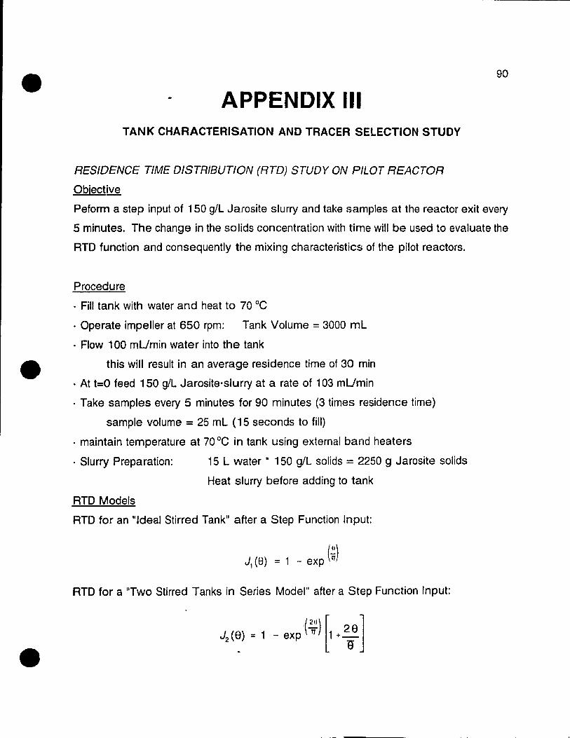
APPENDIX III TANK CHARACTERISATION AND TRACER SELECTION STUDY

RESIDENCE TIME DISTRIBUTION (RTO) STUDY ON PILOT REACTOR

Objective

90

Peform a step input of 150 g/L Jarosite slurry and take samples at the reactor exit every

5 minutes. The change in the solids concentration with time will be used to evaluate the

RTO function and consequently the mixing characteristics of the pilot reactors.

Procedure

· Fil! tank with water and heat to 70 oC

· Operate impeller at 650 rpm: Tank Volume = 3000 ml

· Flow 100 mUmin water into the tank

this will result in an average residence time of 30 min

· At t=o feed 150 g/l Jarosite·slurry at a rate of 103 mUmin

· Take samples every 5 minutes for 90 minutes (3 times residence time)

sample volume = 25 ml (15 seconds to fill)

· maintain temperature at 70 oC in tank using external band heaters

· Siurry Preparation: 15 L water * 150 g/l solids = 2250 9 Jarosite solids

Heat slurry before adding to tank

RTO Models

RTO for an "Ideal Stirred Tank" after a Step Function Input:

~(e) = 1 - exp(~)

RTO for a "Two Stirred Tanks in Series Model" after a Step Function Input:

J,(8) = 1 -exp(~') [1. ~ ]

• 91

STEP CHANGE EXPERIMENTAL RESUL TS

TIME SOLI OS CONG, RTD FUNCTION J(a) (a AVG = 30 min)

(min) (g/L) EXPERIMENTAL IDEAL STA 2 STA in Senes

0 0,0902 0,001 0,000 0,000

2 02290 0,040 0,064 0,008

5 0.4703 0,107 0.154 0,045

10 0,8769 0220 0.283 0,144

15 12608 0326 0,393 0,264

20 1 6111 0.423 0.487 0,385 -25 1,9244 0,510 0565 0.496

30 2,2093 0589 0,632 0,594

35 2,4278 0,650 0.689 0.677

40 2,6256 0,705 0,736 0,745

• 45 2,8072 0,755 0,777 0,801

50 2,9397 0,792 0.811 0,845

55 3,0602 0,826 0,840 0,881

60 3,1790 0,859 0.865 0,908

65 3,2911 0890 0,885 0,930

70 3,3653 0,910 0.903 0,947

75 3.4440 0,932 0.918 0.960

80 3,5135 0.951 0.931 0,969

85 3,5578 0,964 0.941 0.977

90 3,6036 0,976 0950 0,983

95 36505 0989 0958 0,987

100 ~fiRR~ 1.000 o ~fi4 o ~~O

•

• COMPARISON OF IDEAL REACTOR RESPONSE WITH EXPERIMENTAL REACTOR

RTD Fnl J(O) 1~'-------~~ __ ~-~~

1 - --

0.8

0.8

0.4

0.2

--*- EXPERIMENTAL

- IDEAL STR

- - 2 STR ln SERIES

o ro ~ ~ ~ ~ ~ ro ~ ~ ~ TIME (min)

92

From the above figure, we can see that the pilot scale reactor configuration can be

• closely approximated by a ideal stirred tank reactor model.

JAROS/TE BATCH TEST RESUL TS FOR TRACER SELECTION

If we wish to eventually model the industrial jarosite reactors, it will be necessary to have

an idea of the mixing characteristics in these tanks. A method for determining the state

of mixing is to perform a residence time distribution (RTO) study. This can be carried out

by the step of impulse addition of a tracer at the reactor inlet.

An ideal tracer would be inert and would be readily detected in the exit stream. In the

case of the jarosite conversion circuit, the selection of an appropriate tracer is a difficult

task since jarosite tends to react with many species. It was postulated that lithium

sulphate would remain inert during jarosite precipitation. To verify this assumption, a

batch test was carried out to simulate the jarosite conversion process. In this test a

known quantity of lithium sulphate was added (Li2S04.H20) to a beaker. The analytical

• results, clearly show that lithium sulphate was not present in the solids. If we refer to the

•

•

•

93

figure below, we note that the lithium concentration remained essentially unchanged

during the course of the experiment.

Concentration Profiles for Batch Jaroslte Tracer Test

Fe (g/L) & U (mg/L) Zn (gJL) ~=~---------------------------------,140

-7n. .".."."., •

. ... .... A': .. -130 ",'" 30- .... ... .. ... ' ...... .... .. .........

.' ,+ - - - ~' ,.-------i

. , . . . ;;t.:.----f'

•• " ,.," 0. 20t-

'.

, , , ··-FeS+

+Zn2+ 120

~:' ,+----+" 10 !-~"i<' .......... ~:.: ...• _"... . ....... '- 110 ." ........

1 2 346

TlME (hours)

8

o ••••••• .....

7

From these results we are able to conclude that lithium sulphate is inert under these

conditions.

We were surprised to find traces (3 ppm) of lithium already present in the initial plant

solution. Consequently further evaluations will be required in order to determine how the

lithium concentration varies in the circuit. If the variance is too large compared to the

concentration for the tracer added then an alternate tracer must be employed.

Annther key issue in tracer selection deals with its effect on the cell house where the Linc

electro-deposition OCCUI s. It is weil documented that even small amounts of certain

elements will have a deleterious effect on zinc plating efficiency. To ensure that lithium

would not interfere in this process an electrolysis test was carried out with 4 ppm lithium

added to the electrolyte. The test results showed that lithium did not effect the plating

efficiency .

•

•

•

94

The final criterion for tracer selection is that it not be too expensive and that a reliable

analytical technique be élvailable. Recently, a technique was developed using an ICP

(Inductively Coupled Plasma) machine to analyze lithium in trie presence 01 high iion and

zinc concentrations. The results showed that lithium could be analyzed above 20 ppb

with a precision of +/- 3.3% and an accuracy of 92%.

DETERMINATION OF THE EVAPORATION RATE

Objective

ln order to calculate the exit flow from the pilot reactors, a mass balance calculation

around the reactors was carried out. To perform this calculation it was important to

quantify the amount of water evaporating from these covered reactors.

Procedure

• FiJI reactor with jarosite filtrate

• Flow approximately 45 mUmin of the jarosite filtrate into the reactor

• Heat reactor to 9SoC

• Measure the inlet and the outlet flows

Results

Inlet flow = 59.S7 g/min

Outlet flow = 57.64, 5S.07, 48.96 = 54.89 g/min average

Evaporation Rate = 59.87 - 54.S9 = 4.9S g/min +/- 4.19 (+/- 103.2%)

Evaporation Rate used in Mass Balance Calculations: 5.0 g/min

•

•

•

APPENDIX IV ZINC FERRITE AND JAROSITE SOLIDS

JAROS/TE SLURRY STABILITY TESTS

Objective

95

Since there is a concern that the jarosite seeds will react with the jarosite solution during

storage, it is important to quantify the stability of the prepared jarosite slurry.

Procedure

· Prepare a mixture of 33% jarosite slurry by mlxing 1.7 Lof jarosite solution with 2.3 kg

of filtered jarosite solids

· The jarosite solution, which is the Thickener 11 over-fJow solution fram CEZinc, has a

density of 1.302 g/mL and contains approxirnately 25 glL H2S04 , 85 g/L Zn and 6 g/L Fe.

The jarosite solids conta in 35.5% moisture and approximately 30% Fe and 2.5% Zn .

· Sam pIe the slurry and filter. Assay filtrate and solids for zinc, and iron and titrate filtrate

to obtain the sulphuric acid concentration.

JAROS/TE SLURRY STABILITY Changes in Filtrats Composition

'T~~~ ~ ~:~._ ~.nc_ (o/L) Zn2' c.n~ (0/LI7. -------.~

115 ............................................................................ ~... .... ......... ........ ......... .. .......................... e8 ~ ~

..... Zn •• ~*----------

10 . -t--... .,. ............................. .. . . ....... BD

.... Hase ..

15J....--:.~ ... ":'"'. '"':" .. ::::: .... "':': .. ::"' .. ~ .. -: .. :.-: ... ::-" .... ~ .. ~+~.~ ... :_:---:--:-::-~:...... ..... ......... .......... 88 ....................

0~----L-----~----~----~----~----~----~80

134 687 8 DAY

• JAROS/TE SLURRY STAS/LITY Changes in Solids Composition

F. (~) Zn ('It) 32.-----------------------------------------~2.7

~ ~ 31 fo-; ••• • ... .

30 f- .............. .

28 _ ...... .

2.8

. 2.CS

- 2.4

28~----~----~----~----~----~------~--~2.3

1234578 DAY

96

• From the previous figures, it was concluded that the jarosite solution will begin to leach

the jarosite solids after a period of 5 days. This is shown through the reduction in acid

concentration with a corresponding increase in the zinc and iron concentrations in the

solution. Furthermore, the reduction in the percent zinc in the solids further confirms that

zinc is being leached during storage. No information can be drawn trom the percent iron

in the solids assays as these data were erratic.

•

The results from this test have shown that we can prepare the jarosite slurry the day

before a pilot experiment but the prepared slurry must be discarded after being stored for

over 5 days. Furthermore, we can be assured that the composition of the jarosite slurry

does not change during the course of the pilot experiments which have a duration of 24

hours .

•

•

•

97

ZINC FERRITE SOUDS PREPARATION PROCEDURE

Objective

Since the zinc ferrite solids from CEZinc contain up to 60% jarosite seeds, it was

necessary to produce our own zinc ferrite solids using calcine solids from CEZinc. The

resulting solids will not contain any jarosite seed but can be considered as industrial zinc

ferrite since we are using industrial calcine for their preparation.

Procedure

To produce 15 kg of Zn Femle solids, Il IS necessary 10 leach 50 kg of calcine. The ratio of ZinC femle 10 calcine IS

approxlmalely 31% Calcine conlalns approxlmately 60% zinc oXldes and 24% zinc femtes.

FiJI a 250 L sllrred lank reaclor wllh 150 L of cold waler. Reaclor should be equipped wlth some over·head ventilation.

Slart Impe 11er

Add ha If of Ihe calcine (25 kg) and slowly pump approximately 12 L of 96% sulphunc acid into the reactor. The

tempe rature will begin to rise .

Slowly add remalning calcine and continue to pump another 10-12 Lof aCld until the pH is stable between 1.8 to 2.0

(don't forget to adjust the temperature compensator in the pH meter). Under these conditions ail of the zinc oxides

should be leached Since the temperature do es flse rapidly, add some cold water to cool.

Verlfy aCldity by taklng a sample. It should be close to 5 g/L If the aCldlty 15 not hlgh enough « 5 g/L) then femc

hydroxide formation will occur and these solids are dllhcult la IIlter.

Allow reagents ta reacl lor 1 hour

Add co Id water to fIIl reactor ta 6 Inches from the top. Turn off agitation.

Let slurry seille for 30 minutes and then remove 50 L of the supernatant. Replace with cold water. (This will reduce the

concentration 01 the zinc and iron ln solution which are probably close ta the saturation point).

Add 5L of 0.5 g1L Percol 351 flocculent and agltate for 2 minutes.

Reduce agitation and start to 1111er the slurry through a 1111er press. Once the press IS full wash the solids by passlng

water through the press.

The 1111er press should be able ta hold ail 01 the sollds ln Ihe 250 L reactor.

Remove sollds Irom the press and determine the % mOlsture lor the batch .

•

•

•

98

COMPOUND DET~RMINA TlON

Objective

The zinc ferrite solids, used in the pilot experiments, were produced in batches as

outlined in Appendix V. Since one batch only provided enough solids for one pilot

experiment, it was important to determine what solid compounds were present in each

batch since it was difficult to prepare each batch in exactly the same way.

Assumptions

• 100 9 Basis

• Assume: 100 % of the Zn in the solids is present as ZnO.Fe20 3

100 % of the Pb in the solids is present as PbS04

TEST B : Zn Ferrite Batch #2

• Assays: 25.95 % Zn 45.33% Fe 2.79 % Pb

• Calculation:

25.95 9 Zn -->

45.33 9 Fe - 44.33 9 Fe -->

95.69 9 ZnO.Fep3

1.00 9 Fe (remalnlng)

1.91 9 Fe(OH)3 If remaining Fe is as Fe(OHh -->

2.79 9 Pb --> 4.08 9 PbSO~

TOTAL MASS --> 101.68 9

• Composition of Batch #2:

• Assays: 24.97 % Zn

• Composition of Batch #3:

94.1 % ZnO.Fep3

1.9 % Fe(OHb

4.0 % PbSO~

0.0 % Other

TEST C : Zn Ferrite Batch #3

45.12% Fe 2.37 % Pb

91.9 % ZnO.Fep3 35 % PbSO~

4 7 % Fe(OH)3 00 % Other

--> 44.33 9 Fe

•

•

•

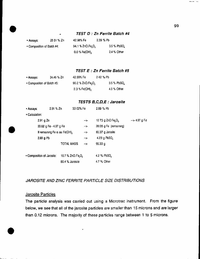
• Assays: 25 51 % Zn

• Composition of Batch #4:

• Assays: 24.46 % Zn

• Composition of Batch #5:

• Assays: 2.91 % Zn

• Calculation:

2.91 9 Zn

33.02 9 Fe - 4.97 9 Fe

If remalnlng Fe 15 as Fe(OHh

2.89 9 Pb

TEST D : Zn Ferrite 8atch #4

42.98% Fe 2.39 % Pb

94.1 % ZnO.Fe203 3.5 % PbSO.

0.0 % Fe(OHh 2.4 % Other

TEST E : Zn Ferrite Batch #5

42.99% Fe

90.2 % ZnO.Fe203

2.3 % Fe(OH)3

242 % Pb

3.5 % PbSO.

4.0 % Other

TESTS 8,C,D,E : Jarosite

3302% Fe 2.89 % Pb

--> 1073 9 ZnO FeP3

--> 28.05 9 Fe (remalmng)

--> 80.37 9 Jarosite

--> 4.23 9 PbSO.

TOTAL MASS --> 95.33 9

• Composition of Jarosite: 10.7 % ZnO.Fe203 4.2 % PbSO.

80.4 % Jaroslte 4.7 % Other

--> 4.97 9 Fe

JARDSITE AND ZINC FERRITE PARTleLE SIZE DISTRIBUTIONS

Jarosite Particles

99

The particle analysis was carried out using a Microtrac instrument From the figure

below, we see that ail of the jarosite particles are smaller than 15 microns and are larger

than 0.12 microns. The majority of these particles range between 1 to 5 microns .

•

•

•

Jarosite Particle Size Distribution

Percent 20r-------------·--------------~=---~-------+100

+ -+

80 16

+ ""*"" Walaht ..

+ Cumulatl_ .. 10

60

40

6 20

o 0 o 1 2 3 4 5 6 7 8 g 10 11 12 13 14 15

Augu.' 1all1 •• mpla

Zinc Ferrite Particles

100

It was attempted to determine the partiele size distribution of the industrial zinc ferrite

particles by wet sieve analysis. This analysis was inconclusive since over 860/0 of the

partiel es were srnaller than 25 microns (using a 500 mesh sieve) .

•

•

•

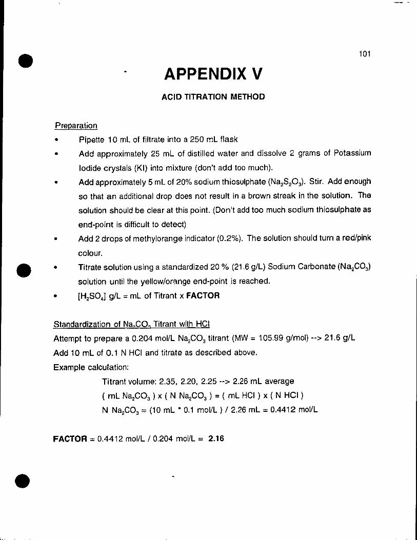
101

APPENDIX V ACID TITRATION METHOD

Preparation

• Pipette 10 ml of filtrate into a 250 ml flask

• Add approximately 25 ml of distilled water and dissolve 2 grams of Potassium

lodide erystals (KI) into mixture (don't add too much).

• Add approximately 5 ml of 20% sodium thiosulphate (Na2S20 3). Stir. Add enough

so that an additional drop does not result in a brown streak in the solution. The

solution should be clear at this point. (Don't add too much sodium thiosulphate as

end-point is difficult to deteet)

• Add 2 drops of methylorange indicator (0.2%). The solution should turn a red/pink

eolour .

• Titrate solution using a standardized 20 % (21.6 g/l) Sodium Carbonate (Na2C03)

solution until the yellow/or::tnge end-point is reached.

• [H2S04] g/l = ml of Titrant x FACTOR

Standardization of Na2C03 Titrant with HCI

Attempt to prepare a 0.204 mol/l Na2C03 titrant (MW = 105.99 g/mol) --> 21.6 g/l

Add 10 ml of 0.1 N HCI and titrate as described above.

Example calculation:

Titrant volume: 2.35, 2.20, 2.25 --> 2.26 ml average

( ml Na2C03 ) x ( N Na2C03 ) = ( ml HCI ) x ( N Hel)

N Na2C03 = (10 ml * 0.1 mol/L) / 2.26 ml = 0.4412 mol/l

FACTOR = 0.4412 mol/l / 0.204 mol/l = 2.16

•

•

•

102

APPENDIX VI TEST FOR COMPARING THE MEANS OF TWO VARIABLES

Hypothesis:

Test:

The ensemble mean (expected value) of A is

significantly different from the ensemble mean

of B

If the difference between the sample means is greater th an the right hand side of the

inequality th en the hypothesis is accepted.

Assumption: and these ensemble variances are bath unknown

Sample statistics

Number of samples in A:

Variable A, sample i:

Sam pie Mean:

Sam pie Variance:

Degrees of Freedom:

Pooled Sam pie Variance:

VA"'VB

•

•

Sample CalculatiÇ.n:

TEST B, TANK 1: Iron Concentration Data

Initial steady-state: A

Step change steady-state: B

Final steady-state: C

XA = 24.86 g/L nA = 5 VA = 4

Xe = 27.55 g/L ne = 4 ve = 3

Xe = 25.59 g/L ne = 4 ve = 3

SA 2 = 0.730 SA = 0.850

S/ = 0.686 Se = 0.828

Se2 = 0.775 Se = 0.880

Hypothesis: ~lA -j; PB at 95% Confidence:

n = 0.450

= XA - XB

a = 0.05

v=7

to 975 = 2.365

sp = 0.843

Left hand side of equation

Right hand side of equation = 2.365 x 0.843 x 0.45° 5

Since 2.69 > 1.34 the hypothesis is satisfied

= 2.69

= 1.34

103

Therefore, the initial steady-state is significantly different trom the step change steady­

state (as expected)

Hypothesis: ~lA -j; ~le at 95% Confidence: a = 0.05

v=7

sp = 0.866

Left hand side of equation

Right hand side of equation

t0975 = 2.365

n = 0.450

= XA - Xe :; 0.73

= 2.365 x 0.866 X 0.45°·5 = 1.37

Since 0.73 < 1.37 the hypoth~sis is not satisfied

Therefore, the initial steady-state is not signlficantly different from the final steady-state

• (as expected)

•

•

•

APPENDIX VII CALCULATION OF THE IONIC STRENGTH

The ionic strength of a solution is defined by the following equation:

where,

S(2ecies:

Ions:

Assuming:

H+

Zn2+

Fe3+

Cu2+

NH4+

Mg2+

Mn2+

ZnS04

(NH)4S04

c = m, , -1

H2S04

MgS04

1 = 2." C Z2 2~ , ,

( mole, per 1000g salt )

moles, per 1000g solvent

Fe2(S04b CuS04

MgS04

Zn2+ H+ Fe3+ Cu2+ Mn2+ Mg2+ NH4+ S042-

[H2S041 = 49 g/L --> [H+] = 1.01 g/L

IONS sot 19L!J. (mol/L) (mol/L) b 1.01 1.00 0.50 1

89.0 1.36 1.36 2

25.0 0.45 0.68 3

1.5 0.02 0.02 2

4.0 0.22 0.11 1

6.0 0.25 0.25 2

8.0 0.15 0.15 2

TOTAL sot= 3.07 -2

Using above equation: 'j = 12.3

104

Z2 ~

4

9

4

1

4

4

4

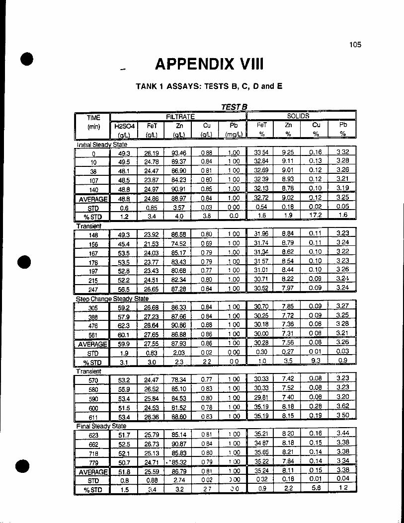
105 • APPENDIX VIII TANK 1 ASSAYS: TESTS B, C, 0 and E

TESTS TIME FILTAATE SOLIDS (min) H2S04 FeT Zn Cu Pb FeT Zn Cu Pb

(0Il) (0Il) (0Il) ( CI!l.) (mail) % % % % Initia 15 d S lea laIe

0 49.3 26.19 93.~6 088 1.00 3354 925 0.16 332 10 49.5 24.78 89.37 0.84 1 00 32.84 9.11 0.13 3.28 38 48.1 24.47 86.90 081 1 00 32.69 9.01 0.12 3.26 107 48.5 23.87 84.23 080 100 3239 8.93 0.12 3.21 140 48.8 24.97 90.91 0.85 1.00 32.13 8.78 0.10 3.19

AVERAGE 48.8 24.86 88.97 0.84 1.00 32.72 9.02 0.12 3.25 STO 0.6 0.85 3.57 0.03 000 0.54 0.18 0.02 0.05

%STO 1.2 3.4 4.0 3.8 0.0 1.6 1.9 17.2 1.6 Translent

148 49.3 23.92 86.58 0.80 100 31.96 8.84 0.11 3.23 156 45.4 21.53 74.52 069 1 00 31.74 8.79 0.11 324

• 167 53.5 24.03 85.17 079 1.00 31.~ 8.62 0.10 322 178 53.5 23.n 83.43 079 100 3157 854 0.10 323 197 52.8 23.43 80.68 0.77 100 31.01 8.44 0.10 326

215 52.2 24.51 82.34 0.80 1.00 30.71 8.22 0.09 3.24 247 56.5 26.65 87.28 0.84 100 30.52 7.97 0.09 3.24

S Ch tep_ al1ge S d S tea Jy tate 305 59.2 26.68 86.33 0.84 100 30.70 7.85 0.09 3.27

388 57.9 27.23 87.66 084 100 30.25 7.72 009 3.25 476 62.3 28.64 90.66 0.88 100 30.18 7.36 0.08 328

561 60.1 27.65 86.88 086 100 30.00 7.31 008 3.21 AVERAGE 59.9 27.55 87.93 0.86 100 30.28 7.56 0.08 3.26

STO 1.9 0.83 2.03 002 000 0.30 0.27 001 0.03

%STO 3.1 3.0 2.3 22 00 1.0 3.5 9.3 0.9 Translent

570 53.2 24.47 78.34 0.77 100 30.33 7.42 0.08 3.23

580 55.9 26.52 85.10 083 100 30.33 7.52 0.08 3.23

590 53.4 25.84 84.53 0.80 100 29.81 740 0.08 3.20

600 5'1.5 24.53 81.52 078 100 35.19 8.18 0.28 3.62 611 53.4 26.36 88.60 083 100 35.19 8.15 0.19 350

Ina ea 1\ F ISt d S tate 623 51.7 25.79 85.14 081 100 35.21 820 0.16 3.44

662 52.5 26.73 90.87 084 100 3487 8.18 0.15 3.38

718 52.1 25.13 85.83 080 100 35.65 8.21 0.14 3.38 • n9 50.7 24.71 " "85.32 079 100 35.22 7.84 0.14 334

AVERAGE 51.8 25.59 86.79 081 100 3524 8.11 015 3.38 STO 0.8 0.88 2.74 002 JOO 032 0.18 0.01 0.04

%STO 1.5 ~1.4 3.2 27 JO 0.9 2.2 5.8 1 2

TESTe 106 • TIME FILTRATE SOLI OS (min) H2S04 FeT Zn Cu Pb FeT Zn Cu Pb

(QILt (QIt) (QIL) (WL) (mwL) % % % % nltlal tead s S tate

0 46.6 26.31 86.82 0.90 1.00 35.92 8.91 028 3.32 28 23.07 75.97 0.78 1.00 35.02 9.05 0.19 3.28 95 46.4 24.25 80.99 083 1.00 36.00 890 0.22 3.26

AVERAGE 46.5 2454 8126 0.84 100 35.6 90 0.2 3.3 STO 0.1 1.6 54 0.1 0.0 05 01 0.0 0.0

%STO 0.3 6.7 67 7.1 0.0 1 5 09 19 a 10 Transient

114 47.5 25.18 83.79 086 1.00 3547 893 0.21 321 124 47.1 24.71 82.54 0.85 1.00 35.'18 8.57 020 323 134 24.16 81.23 084 100 35.76 8.34 0.20 324 144 46.1 22.55 78.33 0.82 1.00 35.68 8.16 0.20 3.23 158 22.89 81.24 0.85 1.00 35.26 7.99 0.20 3.17 , 168 47.0 22.88 82.11 087 100 35.05 7.85 0.19 319 181 21.80 8069 0.85 100 35.45 7.77 019 320 205 47.6 21.63 i'9.86 085 100 35.54 7.65 0.19 3.15 235 21.53 81.36 0.87 100 35.12 7.52 019 3.14

St Ch ep ange ealY ae St d Stt 296 46.6 20.40 76.48 0.82 100 35.22 7.37 0.19 3.13 364 20.63 78.55 084 , 00 3584 735 0.18 316 421 47.1 20.46 78.18 0.84 104 35.16 7.32 0.18 3.10 480 20.30 76.02 0.82 100 35.36 7.31 0.18 3.13 • AVERAGE 46.9 20.45 n.31 0.83 1 01 35.39 7.34 0.19 3.13 STO 0.4 0.14 125 002 002 0.31 0.03 0.00 0.03

%STO 0.8 0.7 1.6 1 8 2.2 0.9 0.4 14 0.8 Translent

549 48.5 22.65 81.11 0.86 100 35.54 7.48 0.19 3.18

558 22.19 79.32 083 1 00 35.38 7.71 019 3.17

569 47.1 22.17 76.80 0.80 100 35.87 7.88 0.19 320

578 23.53 80.24 084 100 3548 790 0.21 3.23

588 47.8 24.05 85.91 0.89 100 35.44 8.00 020 323

604 2422 85.99 089 100 35.95 823 0.20 3.28 622 47.0 24.12 84.25 0.87 100 35.28 8.16 0.19 325

632 23.93 82.03 084 100 35.54 8.31 0.20 3.30

640 46.8 24.85 84.51 087 100 35.64 8.32 0.20 331

661 25.01 84.23 086 100 36.07 8.52 020 332

667 46.1 25.31 83.22 085 100 3630 886 021 341

Inal tea 1\ F' S d S tate 781 27.63 90.42 092 100 36.54 9.12 021 340

842 48.0 27.57 91.36 093 100 3691 9.30 021 344

902 27.30 91.91 094 100 36.76 8.85 0.21 3.41

AVERAGE 48.0 27.5 91.23 093 100 36.7 9.1 0.2 3.4

• STO 0.2 --0.8 00 00 02 0.2 0.0 0.0

%STO 0.6 0.8 1 3 r) 0 05 2.5 1 5 0.7

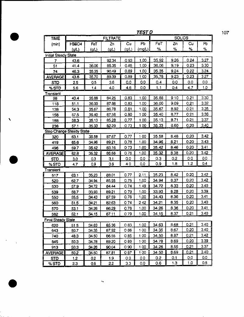
r------------------------ ----- --

• TIME (min) . HaS04 FeT

l' 1 S d St nltia tea ate 7 43.6

51 41.4 36.06

74 46.3 35.35

AVERAGE 43.8 35.70

STO 2.5 0.5

%STO 5.6 1.4

Translent 98 43.4 35.88

118 51.1 36.00

138 54.3 35.67

158 .57.5 35.40 , 188 58.3 35.13

238 57.1 35.33 S Ch tep ange S d S tea ly tate

320 63.1 35.58

419 65.6 34.96

496 59.7 35.42

AVERAGE 62.8 35.32 • STO 3.0 0.3 %8TO 4.7 0.9

Transient 517 63.1 35.23

520 62.7 34.94

530 57.9 34.72

539 58.7 33.93 550 55.5 34.43

560 51.5 34.21

570 53.1 34.26

582 52.1 34.15

Ina tea F IS d S tate 620 515 34.63 643 50.7 34.35 740 48.3 34.50

845 50.3 34.76

913 50.3 34.26

AVERAGE 50.2 34.50

STO 1.2 0.2 %8TO 2.3 0.6

• '.

FILTRATE

92.34 093 85.35 0.85

90.49 0.89

89.39 0.89

3.6 0.0

4.0 4.6

84.25 0.83

87.66 0.83

86.78 0.81

87.56 0.80

85.28 0.77

82.29 073

87.67 0.77

89.21 0.78

83.16 073

86.68 0.76

3.1 0.0 3.6 40

88.01 0.77

85.95 0.75

84.44 0.74

89.21 079 87.59 0.78

82.63 074

86.29 0.78

87.11 079

85.36 083 87.92 086

86.55 085

89.20 089

90.04 090

87.81 087

1.9 00 2.2 3.3

TESTD

Pb

1.00 1.00

1.00

100

0.0

0.0

1.00

1.00 1.00

'00 100

1 00

100

1.00

1.00

1.00

0.0 0.0

2.11

1.00

1 49

1.00 1.00

242

1.00

1.00

1 00

'00 100

100

100

100

00 0.0

FeT %

35.92 36.06

35.35 35.78

0.4

1.1

35.88

36.00

35.67

35.40

35.13

35.33

35.58

34.96

35.42

35.32

0.3 0.9

35.23

34.94

34.72

33.93 34.43

34.21

34.26

34.15

34.63 34.35

34.50

34.78

34.26

3450

0.2 0.6

SOLI OS Zn %

9.26 9.19

9.24 9.23

0.0

0.4

910

9.09

8.92

8.77

8.71

0.60

8.48

8.21

8.46

8.38

0.2 1.8

8.42

8.37

8.33

8.28 8.36

8.35

8.36

8.37

8.68 8.67

8.87

8.69

8.55

8.69

0.1 1.3

Cu %

0.24 0.23

0.22

0.23

0.0

4.7

0.21

0.21

021

021

0.21

0.20

0.20 0.20

0.20

0.20

00 1.2

0.20

0.20

0.20

0.20 0.20

0.20

0.20

0.21

0.21 0.20

0.21

0.20

0.21

0.21

0.0 1.0

107

Pb %

3.27 3.30

3.24

3.27

0.0

1.0

3.30 3.32

3.35

3.36

3.37

3.40

3.42

3.43

3.41

3.42

0.0 0.4

3.42

3.42

3.40

3.39 3.41

3.40

3.41

3.40

3.40 3.40

3.42

3.39

3.37

3.40

0.0 0.5

•

•

•

TIME (min) H2S04

(aIl)

nitial Steadv State 22 50.0 43 48.0 73 45.9

AVERAGE 48.0 STD 2.1

%STD 4.3 Translent

115 47.3 125 46.5 135 46.5 155 41.9 175 47.5 207 44.6

S tep Chan e Steadv 324 42.5 363 428 43.2 453 -AVERAGE 42.!} STO 0.5

%STO 1.2 Transient

536 43.6 545 556 45.8 576 597 46.4 629 675 48.9

Inal tea v F S d S tate 751 800 53.7

862 922 52.7

AVERAGE 53.2 STD 0.7

%STD 1.3

S

FeT (Olt.)

TESTE FILTRATE

Zn Cu Pb FeT (aIL) (aIL) (mail) %

24.58 87.24 0.86 1.00 35.45 23.51 83.32 0.82 1.07 35.33 22.81 80.68 079 1.00 35.32 23.64 83.75 082 1.02 3537

0.9 3.3 0.0 0.0 0.07 3.8 3.9 4.2 4.1 02

23.00 80.92 0.80 1.00 33.12 21.99 78.81 0.77 1.84 33.41 23.10 82.48 0.81 1.10 33.42 21.30 76.80 0.75 1.00 33.63 24.68 88.87 0.88 1.00 33.33 23.35 8447 084 1.00 3346

tate 23.72 85.97 0.85 1.00 33.66 25.41 91.74 0.91 1.00 33.97

24.71 88.88 0.88 1.00 33.83

23.94 87.52 0.87 1.00 33.72 24.44 8853 0.88 1.00 33.8

0.8 2.4 0.0 0.0 0.1 3.2 2.8 2.8 0.0 0.4

25.42 91.50 0.91 1.00 3354 25.72 9030 090 1.00 34.40 25.63 90.21 090 1.00 3390 24.82 85.38 0.85 1.00 33.34 25.57 87.25 087 1.00 33.34

23.75 82.07 0.81 1.00 33.16 24.08 82.73 082 1.94 32.77

26.04 9143 0.90 1.00 32.70 25.33 88.68 0.88 1.00 32.76

25.79 88.78 0.88 1.00 32.90 25.15 8636 085 1.00 32.71

25.58 88.81 088 1.CO 32.8

0.4 2.1 0.0 00 0.1 1.6 2.3 2.3 0.0 0.3

108 SOUDS

Pb °/0

8.55 031 3.15 8.70 0.31 3.15 8,46 0.31 3.16 8.57 0.31 3.15 0.12 0.00 0.01 1,4 0.0 02

8.77 0.22 3.26 9.10 0.22 3.25 9.32 0.22 3.22 9.59 0.23 3.22 9.76 0.23 3.22 10.02 023 3.19

10.07 0.24 3.19 10.34 0.24 3.24 10.46 024 3.20 10.51 0.24 3.18 10.3 0.2 3.2 0.2 0.0 0.0 1.9 1.6 0.8

10.50 0.25 3.18 10,49 0.24 3.24 10.16 0.23 321 9.68 023 3.24 929 0.22 3.30 8.86 0.22 3.30 8.36 0.21 3.31

8.27 0.20 3.36 8.15 0.20 3.33 8.14 0.20 3.31 8.14 0.20 3.34 8.2 0.2 3.3 0.1 0.0 O,&. 0.8 0.8 0.5