Embed Size (px)
Citation preview
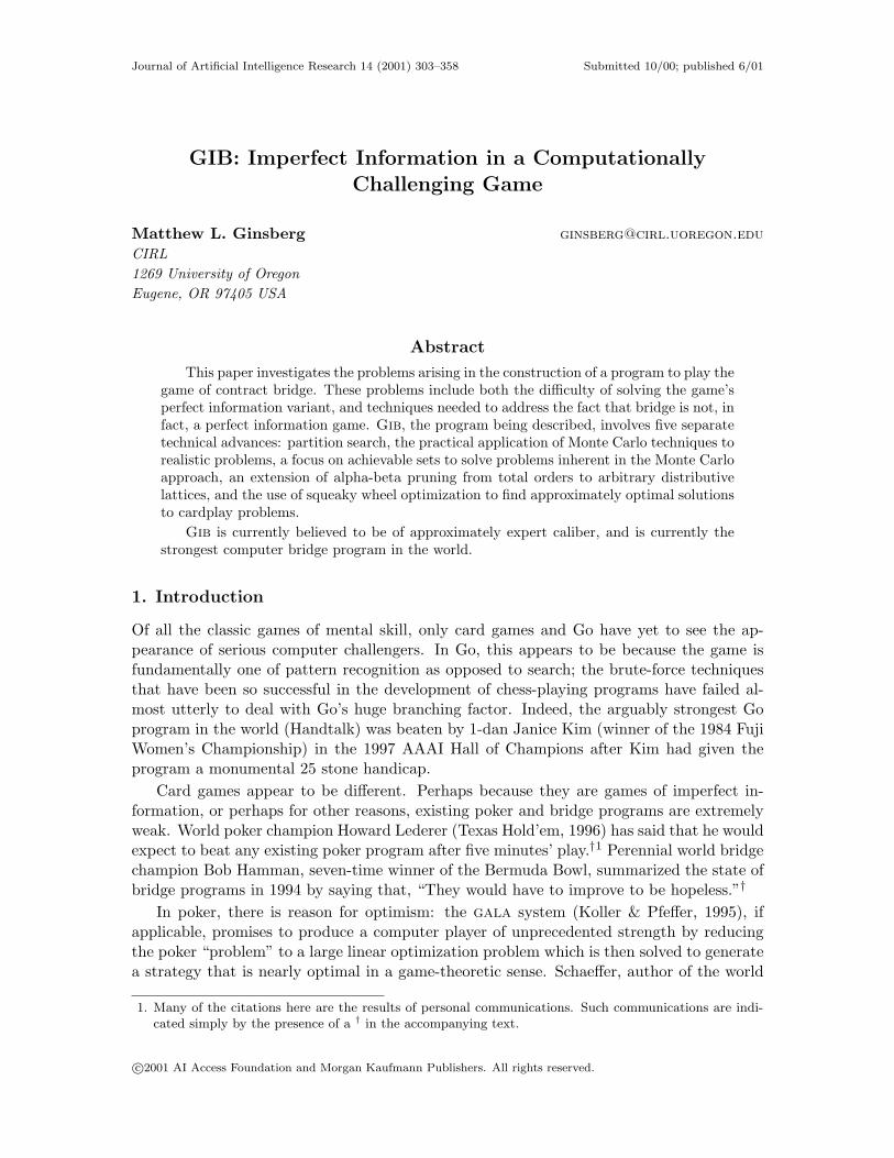
Journal of Artificial Intelligence Research 14 (2001) 303–358 Submitted 10/00; published 6/01
GIB: Imperfect Information in a ComputationallyChallenging Game
Matthew L. Ginsberg [email protected]
CIRL1269 University of OregonEugene, OR 97405 USA
Abstract
This paper investigates the problems arising in the construction of a program to play thegame of contract bridge. These problems include both the difficulty of solving the game’sperfect information variant, and techniques needed to address the fact that bridge is not, infact, a perfect information game. Gib, the program being described, involves five separatetechnical advances: partition search, the practical application of Monte Carlo techniques torealistic problems, a focus on achievable sets to solve problems inherent in the Monte Carloapproach, an extension of alpha-beta pruning from total orders to arbitrary distributivelattices, and the use of squeaky wheel optimization to find approximately optimal solutionsto cardplay problems.
Gib is currently believed to be of approximately expert caliber, and is currently thestrongest computer bridge program in the world.
1. Introduction
Of all the classic games of mental skill, only card games and Go have yet to see the ap-pearance of serious computer challengers. In Go, this appears to be because the game isfundamentally one of pattern recognition as opposed to search; the brute-force techniquesthat have been so successful in the development of chess-playing programs have failed al-most utterly to deal with Go’s huge branching factor. Indeed, the arguably strongest Goprogram in the world (Handtalk) was beaten by 1-dan Janice Kim (winner of the 1984 FujiWomen’s Championship) in the 1997 AAAI Hall of Champions after Kim had given theprogram a monumental 25 stone handicap.
Card games appear to be different. Perhaps because they are games of imperfect in-formation, or perhaps for other reasons, existing poker and bridge programs are extremelyweak. World poker champion Howard Lederer (Texas Hold’em, 1996) has said that he wouldexpect to beat any existing poker program after five minutes’ play.†1 Perennial world bridgechampion Bob Hamman, seven-time winner of the Bermuda Bowl, summarized the state ofbridge programs in 1994 by saying that, “They would have to improve to be hopeless.”†
In poker, there is reason for optimism: the gala system (Koller & Pfeffer, 1995), ifapplicable, promises to produce a computer player of unprecedented strength by reducingthe poker “problem” to a large linear optimization problem which is then solved to generatea strategy that is nearly optimal in a game-theoretic sense. Schaeffer, author of the world
1. Many of the citations here are the results of personal communications. Such communications are indi-cated simply by the presence of a † in the accompanying text.
c©2001 AI Access Foundation and Morgan Kaufmann Publishers. All rights reserved.

Ginsberg
champion checkers program Chinook (Schaeffer, 1997), is also reporting significant successin the poker domain (Billings, Papp, Schaeffer, & Szafron, 1998).
The situation in bridge has been bleaker. In addition, because the American ContractBridge League (acbl) does not rank the bulk of its players in meaningful ways, it is difficultto compare the strengths of competing programs or players.
In general, performance at bridge is measured by playing the same deal twice or more,with the cards held by one pair of players being given to another pair during the replay andthe results then being compared.2 A “team” in a bridge match thus typically consists oftwo pairs, with one pair playing the North/South (N/S) cards at one table and the otherpair playing the E/W cards at the other table. The results obtained by the two pairs areadded; if the sum is positive, the team wins this particular deal and if negative, they loseit.
In general, the numeric sum of the results obtained by the two pairs is converted toInternational Match Points, or imps. The purpose of the conversion is to diminish theimpact of single deals on the total, lest an abnormal result on one particular deal have anunduly large impact on the result of an entire match.
Jeff Goldsmith† reports that the standard deviation on a single deal in bridge is about 5.5imps, so that if two roughly equal pairs were to play the deal, it would not be surprising if oneteam beat the other by about this amount. It also appears that the difference between anaverage club player and an expert is about 1.5 imps (per deal played); the strongest playersin the world are approximately 0.5 imps/deal better still. Excepting gib, the strongestbridge playing programs appear to be slightly weaker than average club players.
Progress in computer bridge has been slow. An incorporation of planning techniques intoBridge Baron, for example, appears to have led to a performance increment of approximately1/3 imp per deal (Smith, Nau, & Throop, 1996). This modest improvement still leavesBridge Baron far shy of expert-level (or even good amateur-level) performance.
Prior to 1997, bridge programs generally attempted to duplicate human bridge-playingmethodology in that they proceeded by attempting to recognize the class into which anyparticular deal fell: finesse, end play, squeeze, etc. Smith et al.’s work on the Bridge Baronprogram uses planning to extend this approach, but the plans continue to be constructedfrom human bridge techniques. Nygate and Sterling’s early work on python (Sterling &Nygate, 1990) produced an expert system that could recognize squeezes but not prepare forthem. In retrospect, perhaps we should have expected this approach to have limited success;certainly chess-playing programs that have attempted to mimic human methodology, suchas paradise (Wilkins, 1980), have fared poorly.
Gib, introduced in 1998, works differently. Instead of modeling its play on techniquesused by humans, gib uses brute-force search to analyze the situation in which it finds itself.A variety of techniques are then used to suggest plays based on the results of the brute-forcesearch. This technique has been so successful that all competitive bridge programs haveswitched from a knowledge-based approach to a search-based approach.
GIB’s cardplay based on brute-force techniques was at the expert level (see Section 3)even without some of the extensions that we discuss in Section 5 and subsequently. Theweakest part of gib’s game is bidding, where it relies on a large database of rules describing
2. The rules of bridge are summarized in Appendix A.
304

GIB: Imperfect information in a computationally challenging game
the meanings of various auctions. Quantitative comparisons here are difficult, although thegeneral impression of the stronger players using GIB are that its overall play is comparableto that of a human expert.
This paper describes the various techniques that have been used in the gib project, asfollows:
1. Gib’s analysis in both bidding and cardplay rests on an ability to analyze bridge’sperfect-information variant, where all of the cards are visible and each side attemptsto take as many tricks as possible (this perfect-information variant is generally referredto as double dummy bridge). Double dummy problems are solved using a techniqueknown as partition search, which is discussed in Section 2.
2. Early versions of gib used Monte Carlo methods exclusively to select an action basedon the double dummy analysis. This technique was originally proposed for cardplayby Levy (Levy, 1989), but was not implemented in a performance program beforegib. Extending Levy’s suggestion, gib uses Monte Carlo simulation for both cardplay(discussed in Section 3) and bidding (discussed in Section 4).
3. Section 5 discusses difficulties with the Monte Carlo approach. Frank et al. havesuggested dealing with these problems by searching the space of possible plans forplaying a particular bridge deal, but their methods appear to be intractable in boththeory and practice (Frank & Basin, 1998; Frank, Basin, & Bundy, 2000). We insteadchoose to deal with the difficulties by modifying our understanding of the game sothat the value of a bridge deal is not an integer (the number of tricks that can betaken) but is instead taken from a distributive lattice.
4. In Section 6, we show that the alpha-beta pruning mechanism can be extended to dealwith games of this type. This allows us to find optimal plans for playing bridge endpositions involving some 32 cards or fewer. (In contrast, Frank’s method is capableonly of finding solutions in 16 card endings.)
5. Finally, applying our ideas to the play of full deals (52 cards) requires solving anapproximate version of the overall problem. In Section 7, we describe the nature ofthe approximation used and our application of squeaky wheel optimization (Joslin &Clements, 1999) to solve it.
Concluding remarks are contained in Section 8.
2. Partition search
Computers are effective game players only to the extent that brute-force search can overcomeinnate stupidity; most of their time spent searching is spent examining moves that a humanplayer would discard as obviously without merit.
As an example, suppose that White has a forced win in a particular chess position,perhaps beginning with an attack on Black’s queen. A human analyzing the position willsee that if Black doesn’t respond to the attack, he will lose his queen; the analysis considersplaces to which the queen could move and appropriate responses to each.
305

Ginsberg
A machine considers responses to the queen moves as well, of course. But it must alsoanalyze in detail every other Black move, carefully demonstrating that each of these othermoves can be refuted by capturing the Black queen. A six-ply search will have to analyzeevery one of these moves five further ply, even if the refutations are identical in all cases.Conventional pruning techniques cannot help here; using α-β pruning, for example, theentire “main line” (White’s winning choices and all of Black’s losing responses) must beanalyzed even though there is a great deal of apparent redundancy in this analysis.3
In other search problems, techniques based on the ideas of dependency maintenance (Stall-man & Sussman, 1977) can potentially be used to overcome this sort of difficulty. As anexample, consider chronological backtracking applied to a map coloring problem. When adead end is reached and the search backs up, no information is cached and the effect is toeliminate only the specific dead end that was encountered. Recording information givingthe reason for the failure can make the search substantially more efficient.
In attempting to color a map with only three colors, for example, thirty countries mayhave been colored while the detected contradiction involves only five. By recording thecontradiction for those five countries, dead ends that fail for the same reason can be avoided.
Dependency-based methods have been of limited use in practice because of the overheadinvolved in constructing and using the collection of accumulated reasons. This problem hasbeen substantially addressed in the work on dynamic backtracking (Ginsberg, 1993) and itssuccessors such as relsat (Bayardo & Miranker, 1996), where polynomial limits are placedon the number of nogoods being maintained.
In game search, however, most algorithms already include significant cached informationin the form of a transposition table (Greenblatt, Eastlake, & Crocker, 1967; Marsland, 1986).A transposition table stores a single game position and the backed up value that has beenassociated with it. The name reflects the fact that many games “transpose” in that identicalpositions can be reached by swapping the order in which moves are made. The transpositiontable eliminates the need to recompute values for positions that have already been analyzed.
These collected observations lead naturally to the idea that transposition tables shouldstore not single positions and their values, but sets of positions and their values. Continuingthe dependency-maintenance analogy, a transposition table storing sets of positions canprune the subsequent search far more efficiently than a table that stores only singletons.
There are two reasons that this approach works. The first, which we have already men-tioned, is that most game-playing programs already maintain transposition tables, therebyincurring the bulk of the computational expense involved in storing such tables in a moregeneral form. The second and more fundamental reason is that when a game ends with oneplayer the winner, the reason for the victory is generally a local one. A chess game can bethought of as ending when one side has its king captured (a completely local phenomenon);a checkers game, when one side runs out of moves. Even if an internal search node is eval-uated before the game ends, the reason for assigning it any specific value is likely to beindependent of some global features (e.g., is the Black pawn on a5 or a6?). Partition searchexploits both the existence of transposition tables and the locality of evaluation for realisticgames.
3. An informal solution to this is Adelson-Velskiy et al.’s method of analogies (Adelson-Velskiy, Arlazarov,& Donskoy, 1975). This approach appears to have been of little use in practice because it is restrictedto a specific class of situations arising in chess games.
306

GIB: Imperfect information in a computationally challenging game
!!!!!!
��� @
@@
aaaaaa
X X X
O O
O X
X X X
O
O O X
X X X
O O
O X
X X O
O X
O X
X X
O O
O X
X X
O
O O X
X X
O O
O X
X X O
O
O X
X X
O
O XO moves
Figure 1: A portion of the game tree for tic-tac-toe
This section explains these ideas via an example and then describes them formally.Experimental results for bridge are also presented.
2.1 An example
Our illustrative examples for partition search will be taken from the game of tic-tac-toe.A portion of the game tree for this game appears in Figure 1, where we are analyzing aposition that is a win for X. We show O’s four possible moves, and a winning responsefor X in each case. Although X frequently wins by making a row across the top of thediagram, α-β pruning cannot reduce the size of this tree because O’s losing options mustall be analyzed separately.
Consider now the position at the lower left in the diagram, where X has won:
X X X
O O
O X
(1)
The reason that X has won is local. If we are retaining a list of positions with knownoutcomes, the entry we can make because of this position is:
X X X
? ? ?
? ? ?
(2)
where the ? means that it is irrelevant whether the associated square is marked with an X, anO, or unmarked. This table entry corresponds not to a single position, but to approximately36 because the unassigned squares can contain X’s, O’s, or be blank. We can reduce thegame tree in Figure 1 to:
307

Ginsberg
@@@ �
��
!!!!!!
��� @
@@
aaaaaa
X X X
? ? ?
? ? ?
X X O
O X
O X
X X
O O
O X
X X
O
O O X
X X
O O
O X
X X O
O
O X
X X
O
O XO moves
Continuing the analysis, it is clear that the position
X X
? ? ?
? ? ?
(3)
is a win for X if X is on play.4 So isX ? ?
? ?
? ? X
and the tree can be reduced to:
����� HHHHH
X X X
? ? ?
? ? ?
X ? ?
? X ?
? ? X
X X
? ? ?
? ? ?
X ? ?
? ?
? ? X
X X
O
O XO moves
Finally, consider the positionX X
?
? ? X
(4)
where it is O’s turn as opposed to X’s. If O moves in the second row, we get an instance of
X X
? ? ?
? ? ?
while if O moves to the upper right, we get an instance of
X ? ?
? ?
? ? X
4. We assume that O has not already won the game here, since X would not be “on play” if the game wereover.
308
GIB: Imperfect information in a computationally challenging game
Thus every one of O’s moves leads to a position that is known to be a win for X, and wecan conclude that the original position (4) is a win for X as well. The root node in thereduced tree can therefore be replaced with the position of (4).
These positions capture the essence of the algorithm we will propose: If player x canmove to a position that is a member of a set known to be a win for x, the given position isa win as well. If every move is to a position that is a loss, the original position is also.
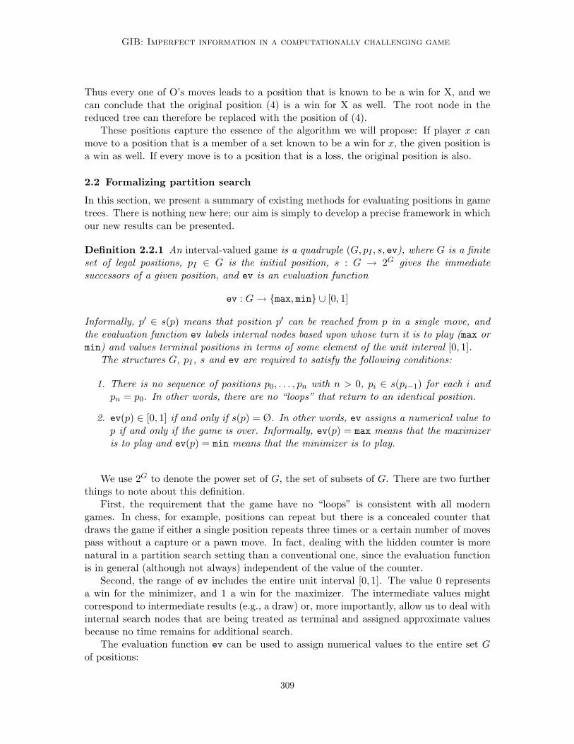
2.2 Formalizing partition search
In this section, we present a summary of existing methods for evaluating positions in gametrees. There is nothing new here; our aim is simply to develop a precise framework in whichour new results can be presented.
Definition 2.2.1 An interval-valued game is a quadruple (G, pI , s, ev), where G is a finiteset of legal positions, pI ∈ G is the initial position, s : G → 2G gives the immediatesuccessors of a given position, and ev is an evaluation function
ev : G → {max, min} ∪ [0, 1]
Informally, p′ ∈ s(p) means that position p′ can be reached from p in a single move, andthe evaluation function ev labels internal nodes based upon whose turn it is to play (max ormin) and values terminal positions in terms of some element of the unit interval [0, 1].
The structures G, pI , s and ev are required to satisfy the following conditions:
1. There is no sequence of positions p0, . . . , pn with n > 0, pi ∈ s(pi−1) for each i andpn = p0. In other words, there are no “loops” that return to an identical position.
2. ev(p) ∈ [0, 1] if and only if s(p) = Ø. In other words, ev assigns a numerical value top if and only if the game is over. Informally, ev(p) = max means that the maximizeris to play and ev(p) = min means that the minimizer is to play.
We use 2G to denote the power set of G, the set of subsets of G. There are two furtherthings to note about this definition.
First, the requirement that the game have no “loops” is consistent with all moderngames. In chess, for example, positions can repeat but there is a concealed counter thatdraws the game if either a single position repeats three times or a certain number of movespass without a capture or a pawn move. In fact, dealing with the hidden counter is morenatural in a partition search setting than a conventional one, since the evaluation functionis in general (although not always) independent of the value of the counter.
Second, the range of ev includes the entire unit interval [0, 1]. The value 0 representsa win for the minimizer, and 1 a win for the maximizer. The intermediate values mightcorrespond to intermediate results (e.g., a draw) or, more importantly, allow us to deal withinternal search nodes that are being treated as terminal and assigned approximate valuesbecause no time remains for additional search.
The evaluation function ev can be used to assign numerical values to the entire set Gof positions:
309
Ginsberg
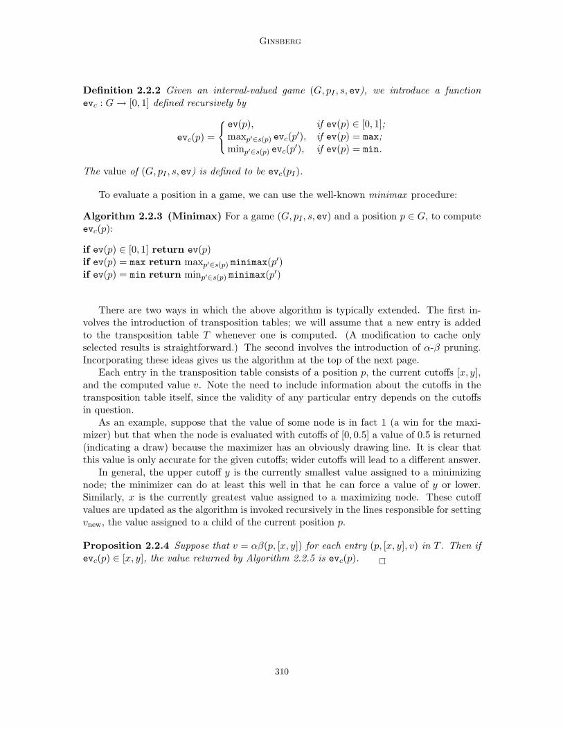
Definition 2.2.2 Given an interval-valued game (G, pI , s, ev), we introduce a functionevc : G → [0, 1] defined recursively by
evc(p) =
ev(p), if ev(p) ∈ [0, 1];maxp′∈s(p) evc(p′), if ev(p) = max;minp′∈s(p) evc(p′), if ev(p) = min.
The value of (G, pI , s, ev) is defined to be evc(pI).
To evaluate a position in a game, we can use the well-known minimax procedure:
Algorithm 2.2.3 (Minimax) For a game (G, pI , s, ev) and a position p ∈ G, to computeevc(p):
if ev(p) ∈ [0, 1] return ev(p)if ev(p) = max return maxp′∈s(p) minimax(p′)if ev(p) = min return minp′∈s(p) minimax(p′)
There are two ways in which the above algorithm is typically extended. The first in-volves the introduction of transposition tables; we will assume that a new entry is addedto the transposition table T whenever one is computed. (A modification to cache onlyselected results is straightforward.) The second involves the introduction of α-β pruning.Incorporating these ideas gives us the algorithm at the top of the next page.
Each entry in the transposition table consists of a position p, the current cutoffs [x, y],and the computed value v. Note the need to include information about the cutoffs in thetransposition table itself, since the validity of any particular entry depends on the cutoffsin question.
As an example, suppose that the value of some node is in fact 1 (a win for the maxi-mizer) but that when the node is evaluated with cutoffs of [0, 0.5] a value of 0.5 is returned(indicating a draw) because the maximizer has an obviously drawing line. It is clear thatthis value is only accurate for the given cutoffs; wider cutoffs will lead to a different answer.
In general, the upper cutoff y is the currently smallest value assigned to a minimizingnode; the minimizer can do at least this well in that he can force a value of y or lower.Similarly, x is the currently greatest value assigned to a maximizing node. These cutoffvalues are updated as the algorithm is invoked recursively in the lines responsible for settingvnew, the value assigned to a child of the current position p.
Proposition 2.2.4 Suppose that v = αβ(p, [x, y]) for each entry (p, [x, y], v) in T . Then ifevc(p) ∈ [x, y], the value returned by Algorithm 2.2.5 is evc(p).
310

GIB: Imperfect information in a computationally challenging game
Algorithm 2.2.5 (α-β pruning with transposition tables) Given an interval-valuedgame (G, pI , s, ev), a position p ∈ G, cutoffs [x, y] ⊆ [0, 1] and a transposition table Tconsisting of triples (p, [a, b], v) with p ∈ G and a ≤ b, v ∈ [0, 1], to compute αβ(p, [x, y]):
if there is an entry (p, [x, y], z) in T return zif ev(p) ∈ [0, 1] then vans = ev(p)if ev(p) = max then
vans := 0for each p′ ∈ s(p) do
vnew = αβ(p′, [max(vans, x), y])if vnew ≥ y then
T := T ∪ (p, [x, y], vnew)return vnew
if vnew > vans then vans = vnew
if ev(p) = min thenvans := 1for each p′ ∈ s(p) do
vnew = αβ(p′, [x,min(vans, y)])if vnew ≤ x then
T := T ∪ (p, [x, y], vnew)return vnew
if vnew < vans then vans = vnew
T := T ∪ (p, [x, y], vans)return vans
2.3 Partitions
We are now in a position to present our new ideas. We begin by formalizing the idea of aposition that can reach a known winning position or one that can reach only known losingones.
Definition 2.3.1 Given an interval-valued game (G, pI , s, ev) and a set of positions S ⊆ G,we will say that the set of positions that can reach S is the set of all p for which s(p)∩S 6= Ø.This set will be denoted R0(S). The set of positions constrained to reach S is the set ofall p for which s(p) ⊆ S, and is denoted C0(S).
These definitions should match our intuition; the set of positions that can reach a set Sis indeed the set of positions p for which some element of S is an immediate successor of p,so that s(p) ∩ S 6= Ø. Similarly, a position p is constrained to reach S if every immediatesuccessor of p is in S, so that s(p) ⊆ S.
Unfortunately, it may not be feasible to construct the R0 and C0 operators explicitly;there may be no concise representation of the set of all positions that can reach S. Inpractice, this will be reflected in the fact that the data structures being used to describe
311

Ginsberg
the set S may not conveniently describe the set R0(S) of all situations from which S canbe reached.
Now suppose that we are expanding the search tree itself, and we find ourselves analyz-ing a particular position p that is determined to be a win for the maximizer because themaximizer can move from p to the winning set S; in other words, p is a win because it isin R0(S). We would like to record at this point that the set R0(S) is a win for the maxi-mizer, but may not be able to construct or represent this set conveniently. We will thereforeassume that we have some computationally effective way to approximate the R0 and C0
functions, in that we have (for example) a function R that is a conservative implementationof R0 in that if R says we can reach S, then so we can:
R(p, S) ⊆ R0(S)
R(p, S) is intended to represent a set of positions that are “like p in that they can reachthe (winning) set S.” Note the inclusion of p as an argument to R(p, S), since we certainlywant p ∈ R(p, S). We are about to cache the fact that every element of R(p, S) is a winfor the maximizer, and certainly want that information to include the fact that p itself hasbeen shown to be a win. Thus we require p ∈ R(p, S) as well.
Finally, we need some way to generalize the information returned by the evaluationfunction; if the evaluation function itself identifies a position p as a win for the maximizer,we want to have some way to generalize this to a wider set of positions that are also wins.We formalize this by assuming that we have some generalization function P that “respects”the evaluation function in the sense that the value returned by P is a set of positions thatev evaluates identically.
Definition 2.3.2 Let (G, pI , S, ev) be an interval-valued game. Let f be any function withrange 2G, so that f selects a set of positions based on its arguments. We will say thatf respects the evaluation function ev if whenever p, p′ ∈ F for any F in the range of f ,ev(p) = ev(p′).
A partition system for the game is a triple (P, R,C) of functions that respect ev suchthat:
1. P : G → 2G maps positions into sets of positions such that for any position p, p ∈P (p).
2. R : G × 2G → 2G accepts as arguments a position p and a set of positions S. Ifp ∈ R0(S), so that p can reach S, then p ∈ R(p, S) ⊆ R0(S).
3. C : G × 2G → 2G accepts as arguments a position p and a set of positions S. Ifp ∈ C0(S), so that p is constrained to reach S, then p ∈ C(p, S) ⊆ C0(S).
As mentioned above, the function P tells us which positions are sufficiently “like” p thatthey evaluate to the same value. In tic-tac-toe, for example, the position (1) where X haswon with a row across the top might be generalized by P to the set of positions
X X X
? ? ?
? ? ?
(5)
312

GIB: Imperfect information in a computationally challenging game
as in (2).The functions R and C approximate R0 and C0. Once again turning to our tic-tac-toe
example, suppose that we take S to be the set of positions appearing in (5) and that p isgiven by
X X
O O
O X
so that S can be reached from p. R(p, S) might be
X X
? ? ?
? ? ?
(6)
as in (3), although we could also take R(p, S) = {p} or R(p, S) to be
X X
O O
O X
∪X X
? ? ?
? ? ?
∪X X
? ? ?
? ? ?
although this last union might be awkward to represent. Note again that R and C arefunctions of p as well as S; the set returned must include the given position p but canotherwise be expected to vary as p does.
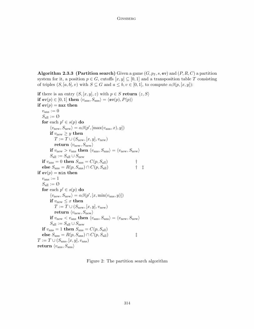
We will now modify Algorithm 2.2.5 so that the transposition table, instead of cachingresults for single positions, caches results for sets of positions. As discussed in the introduc-tion to this section, this is an analog to the introduction of truth maintenance techniquesinto adversary search. The modified algorithm 2.3.3 appears in Figure 2 and returns a pairof values – the value for the given position, and a set of positions that will take the samevalue.
Proposition 2.3.4 Suppose that v = αβ(p, [x, y]) for every (S, [x, y], v) in T and p ∈ S.Then if evc(p) ∈ [x, y], the value returned by Algorithm 2.3.3 is evc(p).
Proof. We need to show that when the algorithm returns, any position in Sans will havethe value vans. This will ensure that the transposition table remains correct.
To see this, suppose that the node being expanded is a maximizing node; the minimizingcase is dual. Suppose first that this node is a loss for the maximizer, having value 0.
In showing that the node is a loss, we will have examined successor nodes that are in setsdenoted Snew in Algorithm 2.3.3; if the maximizer subsequently finds himself in a positionfrom which he has no moves outside of the various Snew, he will still be in a losing position.Since Sall = ∪Snew, the maximizer will lose in any position from which he is constrained tonext move into an element of Sall. Since every position in C(p, Sall) has this property, itis safe to take Sans = C(p, Sall). This is what is done in the first line with a dagger in thealgorithm.
The more interesting case is where the eventual value of the node is nonzero; now inorder for another node n to demonstrably have the same value, the maximizer must haveno new options at n, and must still have some move that achieves the value vans at n.
The first condition is identical to the earlier case where vans = 0. For the second, notethat any time the maximizer finds a new best move, we set Sans to the set of positions that
313
Ginsberg
Algorithm 2.3.3 (Partition search) Given a game (G, pI , s, ev) and (P,R, C) a partitionsystem for it, a position p ∈ G, cutoffs [x, y] ⊆ [0, 1] and a transposition table T consistingof triples (S, [a, b], v) with S ⊆ G and a ≤ b, v ∈ [0, 1], to compute αβ(p, [x, y]):
if there is an entry (S, [x, y], z) with p ∈ S return 〈z, S〉if ev(p) ∈ [0, 1] then 〈vans, Sans〉 = 〈ev(p), P (p)〉if ev(p) = max then
vans := 0Sall := Øfor each p′ ∈ s(p) do
〈vnew, Snew〉 = αβ(p′, [max(vans, x), y])if vnew ≥ y then
T := T ∪ (Snew, [x, y], vnew)return 〈vnew, Snew〉
if vnew > vans then 〈vans, Sans〉 = 〈vnew, Snew〉Sall := Sall ∪ Snew
if vans = 0 then Sans = C(p, Sall) †else Sans = R(p, Sans) ∩ C(p, Sall) † ‡
if ev(p) = min thenvans := 1Sall := Øfor each p′ ∈ s(p) do
〈vnew, Snew〉 = αβ(p′, [x,min(vans, y)])if vnew ≤ x then
T := T ∪ (Snew, [x, y], vnew)return 〈vnew, Snew〉
if vnew < vans then 〈vans, Sans〉 = 〈vnew, Snew〉Sall := Sall ∪ Snew
if vans = 1 then Sans = C(p, Sall)else Sans = R(p, Sans) ∩ C(p, Sall) ‡
T := T ∪ (Sans, [x, y], vans)return 〈vans, Sans〉
Figure 2: The partition search algorithm
314

GIB: Imperfect information in a computationally challenging game
we know recursively achieve the same value. When we complete the maximizer’s loop inthe algorithm, it follows that Sans will be a set of positions from which the maximizer canindeed achieve the value vans. Thus the maximizer can also achieve that value from anyposition in R(p, Sans). It follows that the overall set of positions known to have the valuevans is given by R(p, Sans) ∩ C(p, Sall), intersecting the two conditions of this paragraph.This is what is done in the second daggered step in the algorithm.
2.4 Zero-window variations
The effectiveness of partition search depends crucially on the size of the sets maintained inthe transposition table. If the sets are large, many positions will be evaluated by lookup.If the sets are small, partition search collapses to conventional α-β pruning.
An examination of Algorithm 2.3.3 suggests that the points in the algorithm at whichthe sets are reduced the most are those marked with a double dagger in the description,where an intersection is required because we need to ensure both that the player can makea move equivalent to his best one and that there are no other options. The effectiveness ofthe method would be improved if this possibility were removed.
To see how to do this, suppose for a moment that the evaluation function always returned0 or 1, as opposed to intermediate values. Now if the maximizer is on play and the valuevnew = 1, a prune will be generated because there can be no better value found for themaximizer. If all of the vnew are 0, then vans = 0 and we can avoid the troublesomeintersection. The maximizer loses and there is no “best” move that we have to worry aboutmaking.
In reality, the restriction to values of 0 or 1 is unrealistic. Some games, such as bridge,allow more than two outcomes, while others cannot be analyzed to termination and needto rely on evaluation functions that return approximate values for internal nodes. We candeal with these situations using a technique known as zero-window search (originally calledscout search (Pearl, 1980)). To evaluate a specific position, one first estimates the valueto be e and then determines whether the actual value is above or below e by treating anyvalue v > e as a win for the maximizer and any value v ≤ e as a win for the minimizer. Theresults of this calculation can then be used to refine the guess, and the process is repeated.If no initial estimate is available, a binary search can be used to find the value to withinany desired tolerance.
Zero-window search is effective because little time is wasted on iterations where theestimate is wildly inaccurate; there will typically be many lines showing that a new estimateis needed. Most of the time is spent on the last iteration or two, developing tight boundson the position being considered. There is an analog in conventional α-β pruning, wherethe bounds typically get tight quickly and the bulk of the analysis deals with a situationwhere the value of the original position is known to lie in a fairly narrow range.
In zero-window search, a node always evaluates to 0 or 1, since either v > e or v ≤ e.This allows a straightforward modification to Algorithm 2.3.3 that avoids the troublesomecases mentioned earlier.
315
Ginsberg
2.5 Experimental results
Partition search was tested by analyzing 1000 randomly generated bridge deals and com-paring the number of nodes expanded using partition search and conventional methods.
In addition to our general interest in bridge, there are two reasons why it can be expectedthat partition search will be useful for this game. First, partition search requires that thefunctions R0 and C0 support a partition-like analysis; it must be the case that an analysis ofone situation will apply equally well to a variety of similar ones. Second, it must be possibleto build approximating functions R and C that are reasonably accurate representatives ofR0 and C0.
Bridge satisfies both of these properties. Expert discussion of a particular deal oftenwill refer to small cards as x’s, indicating that it is indeed the case that the exact ranks ofthese cards are irrelevant. Second, it is possible to “back up” x’s from one position to itspredecessors. If, for example, one player plays a club with no chance of having it impactthe rest of the game, and by doing so reaches a position in which subsequent analysis showshim to have two small clubs, then he clearly must have had three small clubs originally.Finally, the fact that cards are simply being replaced by x’s means that it is possible toconstruct data structures for which the time per node expanded is virtually unchanged fromthat using conventional methods.
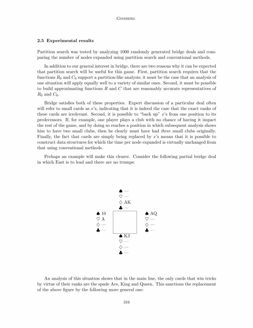
Perhaps an example will make this clearer. Consider the following partial bridge dealin which East is to lead and there are no trumps:
♠ —♥ —♦ AK♣ —
♠ 10 ♠ AQ♥ A ♥ —♦ — ♦ —♣ — ♣ —
♠ KJ♥ —♦ —♣ —
An analysis of this situation shows that in the main line, the only cards that win tricksby virtue of their ranks are the spade Ace, King and Queen. This sanctions the replacementof the above figure by the following more general one:
316

GIB: Imperfect information in a computationally challenging game
♠ —♥ —♦ xx♣ —
♠ x ♠ AQ♥ x ♥ —♦ — ♦ —♣ — ♣ —
♠ Kx♥ —♦ —♣ —
Note first that this replacement is sound in the sense that every position that is aninstance of the second diagram is guaranteed to have the same value as the original. Wehave not resorted to an informal argument of the form “Jacks and lower tend not to matter,”but instead to a precise argument of the form, “In the expansion of the search tree associatedwith the given deal, Jacks and lower were proven never to matter.”
Bridge also appears to be extremely well-suited (no pun intended) to the kind of analysisthat we have been describing; a chess analog might involve describing a mating combinationand saying that “the position of Black’s queen didn’t matter.” While this does happen,casual chess conversation is much less likely to include this sort of remark than bridgeconversation is likely to refer to a host of small cards as x’s, suggesting at least that thepartition technique is more easily applied to bridge than to chess (or to other games).
That said, however, the results for bridge are striking, leading to performance improve-ments of an order of magnitude or more on fairly small search spaces (perhaps 106 nodes).The deals we tested involved between 12 and 48 cards and were analyzed to termination, sothat the depth of the search varied from 12 to 48. (The solver without partition search wasunable to solve larger problems.) The branching factor for minimax without transpositiontables appeared to be approximately 4, and the results appear in Figure 3.
Each point in the graph corresponds to a single deal. The position of the point on thex-axis indicates the number of nodes expanded using α-β pruning and transposition tables,and the position on the y-axis the number expanded using partition search as well. Bothaxes are plotted logarithmically.
In both the partition and conventional cases, a binary zero-window search was used todetermine the exact value to be assigned to the hand, which the rules of bridge constrainto range from 0 to the number of tricks left (one quarter of the number of cards in play).As mentioned previously, hands generated using a full deck of 52 cards were not consideredbecause the conventional method was in general incapable of solving them. The program wasrun on a Sparc 5 and PowerMac 6100, where it expanded approximately 15K nodes/second.The transposition table shares common structure among different sets and as a result, usesapproximately 6 bytes/node.
The dotted line in the figure is y = x and corresponds to the breakeven point relative toα-β pruning in isolation. The solid line is the least-squares best fit to the logarithmic data,and is given by y = 1.57x0.76. This suggests that partition search is leading to an effectivereduction in branching factor of b → b0.76. This improvement, above and beyond that
317

Ginsberg
10
103
105
107
10 103 105 107
Partition
Conventional
p
pp p pppp
pppp
pppppp p
ppp p pp p pppp
pp ppp pp pp
p pp p
pp p
pp
pp ppp pp
pp
p p pppp p
p
pp
pp pp p
p pp pppp pp pp p
p pp p
p
pp p p
pp pp
pp p
p ppp
ppp
pp pp
p p ppp ppp
p p pppp
p pp p pp
p pp
ppp pp p pp
pp p p
ppppp
pp pp
p ppppp
p pppp p pp pp
p ppp pp ppp
pp
p ppp p pp
pp
p pp ppppp
p
pp
pp
pp
pppp
pp
p ppp
pp p
pp p p pp p p
pp p pp
ppp pp p
ppp
ppp ppp p pp p
pp p pp
p
p pp pp pp
p ppp ppp p p
pppp
ppp
pp
p p
pppppp
pp pp
pppp pp ppp
p
p ppp
pppp
pp
p
ppp pp
p
p ppp p pp
pp
p
ppp p p
p
p pp
pp
pp pp ppp
p pp
ppp
pp
ppp pp p
ppp p
ppp
pp
pppp pp
pp p pp
p p pp
pppp
pp
ppppp pp
p ppp
pp p pp pppp
p
p p p
pp
p
p p
p pp pp
p p ppp
ppppp
p
pppp pp
pp ppp p
ppp
p pp
pp pp pp
p
ppppppp
p
ppp
pp p
pppp
pp
pp pp
ppp pp
pp p
p
p
p
p ppppppp
pp ppp p p
p
ppppp
p pp p
pp
pppp pp
pp p
p
p
pp
p ppp
ppp
ppp
ppp
p
pp pp ppppp pp
p
ppp
pp p pp
p
ppp p pp
p
p
ppp pp
ppp
p
pp
ppp pp pp
pp
ppp pp ppp pp
pp
p
p pppp pp pp
p
p
ppp
pppppp p
pp
p pp
pp ppp
pp
pp pppp p p
ppp pp ppp
p
p pp
pp
p
p
pp
p
p
pp
p
p
pp
pp
p
pp
pppp
p p pp p
p
p
p
p p pppp p
pp
p
p
p p
p pp
p
pp
p ppppp
pp
pp
p
pppp p
p
pp p
ppp
ppp pp ppp
pp p
pp
pppppp
pp p
pp p
ppppp
p pp
p
p
p pp
pp
p
pppp p p
p p pp
pp pp ppp p
p
pp p
p
ppp p
pp
ppp
pp p
pp
p p
ppp
pp pp p
p
p
pp
ppp ppp ppp p
p
pp
pp
pp
pp
ppp
pp pp
ppp
pp
p
ppp
p
pp p
p
p
pp pp p
pp
p
pppp
pp ppp
p p
p
pp
pp
ppp
pp
p
pp
p ppp
ppp p ppp
pp
ppp
pp
ppp
p pp
p
p
ppp
p p
pp
p
p p
p
p
p p p ppp p
p ppp
pp
pp
ppp
p
ppp
p pp pppp
pp pp ppp
p
p
p
ppp
pp
pp
p
ppp
p
pp
p
pp
1.57x0.76
Figure 3: Nodes expanded as a function of method
provided by α-β pruning, can be contrasted with α-β pruning itself, which gives a reductionwhen compared to pure minimax of b → b0.75 if the moves are ordered randomly (Pearl,1982) and b → b0.5 if the ordering is optimal.
The method was also applied to full deals of 52 cards, which can be solved while ex-panding an average of 18,000 nodes per deal.5 This works out to about a second of cputime.
3. Monte Carlo cardplay algorithms
One way in which we might use our perfect-information cardplay engine to proceed in arealistic situation would be to deal the unseen cards at random, biasing the deal so that itwas consistent both with the bidding and with the cards played thus far. We could thenanalyze the resulting deal double dummy and decide which of our possible plays was thestrongest. Averaging over a large number of such Monte Carlo samples would allow us todeal with the imperfect nature of bridge information. This idea was initially suggested byLevy (Levy, 1989), although he does not appear to have realized (see below) that there areproblems with it in practice.
Algorithm 3.0.1 (Monte Carlo card selection) To select a move from a candidate setM of such moves:
5. The version of gib that was released in October of 2000 replaced the transposition table with a datastructure that uses a fixed amount of memory, and also sorts the moves based on narrowness (suggestedby Plaat et al. (Plaat, Schaeffer, Pijls, & de Bruin, 1996) to be rooted in the idea of conspiracy search(McAllester, 1988)) and the killer heuristic. While the memory requirements are reduced, the overallperformance is little changed.
318

GIB: Imperfect information in a computationally challenging game
1. Construct a set D of deals consistent with both the bidding and play of the deal thusfar.
2. For each move m ∈ M and each deal d ∈ D, evaluate the double dummy result ofmaking the move m in the deal d. Denote the score obtained by making this moves(m, d).
3. Return that m for which∑
d s(m, d) is maximal.
The Monte Carlo approach has drawbacks that have been pointed out by a variety ofauthors, including Koller† and others (Frank & Basin, 1998). Most obvious among theseis that the approach never suggests making an “information gathering play.” After all,the perfect-information variant on which the decision is based invariably assumes that theinformation will be available by the time the next decision must be made! Instead, thetendency is for the approach to simply defer important decisions; in many situations thismay lead to information gathering inadvertently, but the amount of information acquiredwill generally be far less than other approaches might provide.
As an example, suppose that on a particular deal, gib has four possible lines of play tomake its contract:
1. Line A works if West has the ♠Q.
2. Line B works if East has the ♠Q.
3. Line C defers the guess until later.
4. Line D (the clever line) works independent of who has the ♠Q.
Assuming that either player is equally likely to hold the ♠Q, a Monte Carlo analyzerwill correctly conclude that line A works half the time, and line B works half the time. LineC, however, will be presumed to work all of the time, since the contract can still be made(double dummy) if the guess is deferred. Line D will also be concluded to work all of thetime (correctly, in this case).
As a result, gib will choose randomly between the last two possibilities above, believingas it does that if it can only defer the guess until later (even the next card), it will makethat guess correctly. The correct play, of course, is D.
We will discuss a solution to these difficulties in Sections 5–7; although gib’s defensivecardplay continues to be based on the above ideas, its declarer play now uses stronger tech-niques. Nevertheless, basing the card play on the algorithm presented leads to extremelystrong results, approximately at the level of a human expert. Since gib’s introduction, allother competitive bridge-playing programs have switched their cardplay to similar meth-ods, although gib’s double dummy analysis is substantially faster than most of the otherprograms and its play is correspondingly stronger.
We will describe three tests of GIB’s cardplay algorithms: Performance on a com-mercially available set of benchmarks, performance in a human championship designed tohighlight cardplay in isolation, and statistical performance measured over a large set ofdeals.
319

Ginsberg
For the first test, we evaluated the strength of gib’s cardplay using Bridge Master (BM),a commercial program developed by Canadian internationalist Fred Gitelman. BM contains180 deals at 5 levels of difficulty. Each of the 36 deals on each level is a problem in declarerplay. If you misplay the hand, BM moves the defenders’ cards around if necessary to ensureyour defeat.
BM was used for the test instead of randomly dealt deals because the signal to noise ra-tio is far higher; good plays are generally rewarded and bad ones punished. Every deal alsocontains a lesson of some kind; there are no completely uninteresting deals where the lineof play is irrelevant or obvious. There are drawbacks to testing gib’s performance on non-randomly dealt deals, of course, since the BM deals may in some way not be representativeof the problems a bridge player would actually encounter at the table.
The test was run under Microsoft Windows on a 200 MHz Pentium Pro. As a benchmark,Bridge Baron (BB) version 6 was also tested on the same deals using the same hardware.6
BB was given 10 seconds to select each play, and gib was given 90 seconds to play the entiredeal with a maximum Monte Carlo sample size of 50.7 New deals were generated each timea play decision needed to be made.
These numbers approximately equalized the computational resources used by the twoprograms; BB could in theory take 260 seconds per deal (ten seconds on each of 26 plays),but in practice took substantially less. Gib was given the auctions as well; there was nofacility for doing this in BB. This information was critical on a small number of deals.
Here is how the two systems performed:
Level BB GIB1 16 312 8 233 2 124 1 215 4 13
Total 33 10018.3% 55.6%
Each entry is the number of deals that were played successfully by the program in question.Gib’s mistakes are illuminating. While some of them involve failing to gather informa-
tion, most are problems in combining multiple chances (as in case D above). As BM’s dealsget more difficult, they more often involve combining a variety of possibly winning optionsand that is why GIB’s performance falls off at levels 2 and 3.
At still higher levels, however, BM typically involves the successful development ofcomplex end positions, and gib’s performance rebounds. This appeared to happen to BBas well, although to a much lesser extent. It was gratifying to see gib discover for itself thecomplex end positions around which the BM deals are designed, and more gratifying stillto witness gib’s discovery of a maneuver that had hitherto not been identified in the bridgeliterature, as described in Appendix B.
6. The current version is Bridge Baron 10 and could be expected to perform guardedly better in a test suchas this. Bridge Baron 6 does not include the Smith enhancements (Smith et al., 1996).
7. GIB’s Monte Carlo sample size is fixed at 50 in most cases, which provides a good compromise betweenspeed of play and accuracy of result.
320
GIB: Imperfect information in a computationally challenging game
Experiments such as this one are tedious, because there is no text interface to a com-mercial program such as Bridge Master or Bridge Baron. As a result, information regardingthe sensitivity of gib’s performance to various parameters tends to be only anecdotal.
Gib solves an additional 16 problems (bringing its total to 64.4%) given additionalresources in the form of extra time (up to 100 seconds per play, although that time wasvery rarely taken), a larger Monte Carlo sample (100 deals instead of 50) and hand-generatedexplanations of the opponents’ bids and opening leads. Each of the three factors appearedto contribute equally to the improved performance.
Other authors are reporting comparable levels of performance for gib. Forrester, workingwith a different but similar benchmark (Blackwood, 1979), reports8 that gib solves 68% ofthe problems given 20 seconds/play, and 74% of them given 30 seconds/play. Deals wheregib has outplayed human experts are the topic of a series of articles in the Dutch bridgemagazine IMP (Eskes, 1997, and sequels).9 Based on these results, gib was invited toparticipate in an invitational event at the 1998 world bridge championships in France; theevent involved deals similar to Bridge Master’s but substantially more difficult. Gib joineda field of 34 of the best card players in the world, each player facing twelve such problemsover the course of two days. Gib was leading at the halfway mark, but played poorly onthe second day (perhaps the pressure was too much for it), and finished twelfth.
The human participants were given 90 minutes to play each deal, although they werepenalized slightly for playing slowly. GIB played each deal in about ten minutes, using aMonte Carlo sample size of 500; tests before the event indicated little or no improvementif gib were allotted more time. Michael Rosenberg, the eventual winner of the contest andthe pre-tournament favorite, in fact made one more mistake than did Bart Bramley, thesecond place finisher. Rosenberg played just quickly enough that Bramley’s accumulatedtime penalties gave Rosenberg the victory. The scoring method thus favors GIB slightly.
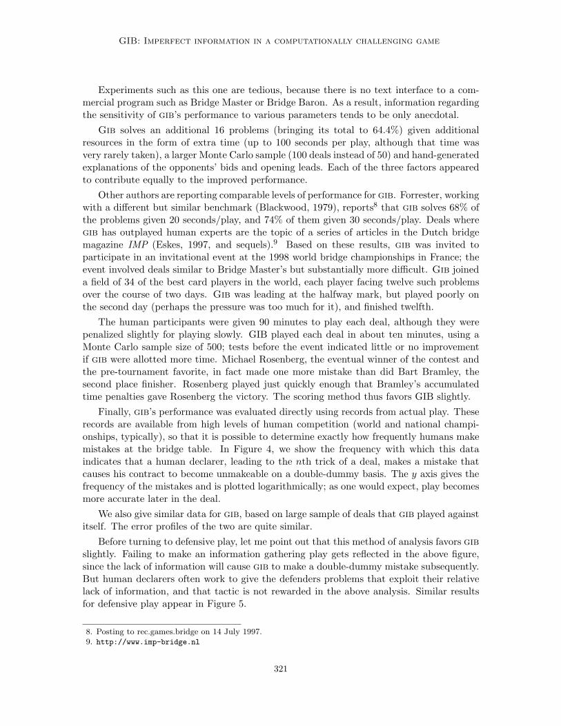
Finally, gib’s performance was evaluated directly using records from actual play. Theserecords are available from high levels of human competition (world and national champi-onships, typically), so that it is possible to determine exactly how frequently humans makemistakes at the bridge table. In Figure 4, we show the frequency with which this dataindicates that a human declarer, leading to the nth trick of a deal, makes a mistake thatcauses his contract to become unmakeable on a double-dummy basis. The y axis gives thefrequency of the mistakes and is plotted logarithmically; as one would expect, play becomesmore accurate later in the deal.
We also give similar data for gib, based on large sample of deals that gib played againstitself. The error profiles of the two are quite similar.
Before turning to defensive play, let me point out that this method of analysis favors gibslightly. Failing to make an information gathering play gets reflected in the above figure,since the lack of information will cause gib to make a double-dummy mistake subsequently.But human declarers often work to give the defenders problems that exploit their relativelack of information, and that tactic is not rewarded in the above analysis. Similar resultsfor defensive play appear in Figure 5.
8. Posting to rec.games.bridge on 14 July 1997.9. http://www.imp-bridge.nl
321

Ginsberg
0.0001
0.001
0.01
0.1
0 2 4 6 8 10 12
P(err)
trick
humanGIB
Figure 4: Gib’s performance as declarer
1e-05
0.0001
0.001
0.01
0.1
0 2 4 6 8 10 12
P(err)
trick
humanGIB
Figure 5: Gib’s performance as defender
322

GIB: Imperfect information in a computationally challenging game
There are two important technical remarks that must be made about the Monte Carloalgorithm before proceeding. First, note that we were cavalier in simply saying, “Constructa set D of deals consistent with both the bidding and play of the deal thus far.”
To construct deals consistent with the bidding, we first simplify the auction as observed,building constraints describing each of the hands around the table. We then deal handsconsistent with the constraints using a deal generator that deals unbiased hands givenrestrictions on the number of cards held by each player in each suit. This set of deals isthen tested to remove elements that do not satisfy the remaining constraints, and each of theremaining deals is passed to the bidding module to identify those for which the observed bidswould have been made by the players in question. (This assumes that gib has a reasonableunderstanding of the bidding methods used by the opponents.) The overall dealing processtypically takes one or two seconds to generate the full set of deals needed by the algorithm.
Now the card play must be analyzed. Ideally, gib would do something similar to what itdoes for the bidding, determining whether each player would have played as indicated on anyparticular deal. Unfortunately, it is simply impractical to test each hypothetical decisionrecursively against the cardplay module itself. Instead, gib tries to evaluate the probabilitythat West (for example) has the ♠K (for example), and to then use these probabilities toweight the sample itself.
To understand the source of the weighting probabilities, let us consider a specific exam-ple. Suppose that in some particular situation, gib plays the ♠5. The analysis indicatesthat 80% of the time that the next player (say West) holds the ♠K, it is a mistake for Westnot to play it. In other words, West’s failure to play the ♠K leads to odds of 4:1 that hehasn’t got it.
These odds are now used via Bayes’ rule to adjust the probability that West holds the♠K at all. The probabilities are then modified further to include information revealed bydefensive signalling (if any), and the adjusted probabilities are finally used to bias the MonteCarlo sample. The evaluation
∑d s(m, d) in Algorithm 3.0.1 is replaced with
∑d wds(m, d)
where wd is the weight assigned to deal d. More heavily weighted deals thus have a largerimpact on gib’s eventual decision.
The second technical point regarding the algorithm itself involves the fact that it needsto run quickly and that it may need to be terminated before the analysis is complete. For theformer, there are a variety of greedy techniques that can be used to ensure that a move mis not considered if we can show
∑d s(d,m) ≤ ∑
d s(d, m′) for some m′. The algorithm alsouses iterative broadening (Ginsberg & Harvey, 1992) to ensure that a low-width answeris available if a high-width search fails to terminate in time. Results from the low- andhigh-width searches are combined when time expires.
Also regarding speed, the algorithm requires that for each deal in the Monte Carlosample and each possible move, we evaluate the resulting position exactly. Knowing simplythat move m1 is not as good as move m2 for deal d is not enough; m1 may be better than m2
elsewhere and we need to compare them quantitatively. This approach is aided substantiallyby the partition search idea, where entries in the transposition table correspond not to singlepositions and their evaluated values, but to sets of positions and values. In many cases,m1 and m2 may fall into the same entry of the partition table long before they actuallytranspose into one another exactly.
323

Ginsberg
4. Monte Carlo bidding
The purpose of bidding in bridge is twofold. The primary purpose is to share informationabout your cards with your partner so that you can cooperatively select an optimal finalcontract. A secondary purpose is to disrupt the opponents’ attempt to do the same.
In order to achieve this purpose, a wide variety of bidding “languages” have been de-veloped. In some, when you suggest clubs as trumps, it means you have a lot of them. Inothers, the suggestion is only temporary and the information conveyed is quite different.In all of these languages, some meaning is assigned to a wide variety of bids in particularsituations; there are also default rules that assign meanings to bids that have no specificallyassigned meanings. Any computer bridge player will need similar understandings.
Bidding is interesting because the meanings frequently overlap; there may be one ormore bids that are suitable (or nearly so) on any particular set of cards. Existing computerprograms have simply matched possible bids against large databases giving their meanings,searching for that bid that best matches the cards that the machines hold. World championChip Martel reports† that human experts take a different approach.10,11
Although expert bidding is based on a database such as that used by existing programs,close decisions are made by simulating the results of each candidate action. This involvesprojecting how the bidding is likely to proceed and evaluating the play in one of a variety ofpossible final contracts. An expert gets his “judgment” from a Monte Carlo-like simulationof the results of possible bids, often referred to in the bridge-playing community as a Borelsimulation (so named after the first player to describe the method). Gib takes a similartack.
Algorithm 4.0.2 (Borel simulation) To select a bid from a candidate set B, given adatabase Z that suggests bids in various situations:
1. Construct a set D of deals consistent with the bidding thus far.
2. For each bid b ∈ B and each deal d ∈ D, use the database Z to project how the auctionwill continue if the bid b is made. (If no bid is suggested by the database, the playerin question is assumed to pass.) Compute the double dummy result of the eventualcontract, denoting it s(b, d).
3. Return that b for which∑
d s(b, d) is maximal.
As with the Monte Carlo approach to card play, this approach does not take into accountthe fact that bridge is not played double dummy. Human experts often choose not to makebids that will convey too much information to the opponents in order to make the defenders’task as difficult as possible. This consideration is missing from the above algorithm.12
10. The 1994 Rosenblum Cup World Team Championship was won by a team that included Martel andRosenberg.
11. Frank suggests (Frank, 1998) that the existing machine approach is capable of reaching expert levels ofperformance. While this appears to have been true in the early 1980’s (Lindelof, 1983), modern expertbidding practice has begun to highlight the disruptive aspect of bidding, and machine performance is nolonger likely to be competitive.
12. In theory at least, this issue could be addressed using the single-dummy ideas that we will present insubsequent sections. Computational considerations currently make this impractical, however.
324

GIB: Imperfect information in a computationally challenging game
There are more serious problems also, generally centering around the development ofthe bidding database Z.
First, the database itself needs to be built and debugged. A large number of rules needto be written, typically in a specialized language and dependent upon the bridge expertiseof the author. The rules need to be debugged as actual play reveals oversights or otherdifficulties.
The nature and sizes of these databases vary enormously, although all of them representvery substantial investments on the part of the authors. The database distributed withmeadowlark bridge includes some 7300 rules; that with q-plus bridge 2500 rulescomprising 40,000 lines of specialized code. Gib’s database is built using a derivative of theMeadowlark language, and includes about 3000 rules.
All of these databases doubtless contain errors of one sort or another; one of the nicethings about most bidding methods is that they tend to be fairly robust against such prob-lems. Unfortunately, the Borel algorithm described above introduces substantial instabilityin gib’s overall bidding.
To understand this, suppose that the database Z is somewhat conservative in its actions.The projection in step 2 of Algorithm 4.0.2 now leads each player to assume its partner bidsconservatively, and therefore to bid somewhat aggressively to compensate. The partnershipas a whole ends up overcompensating.
Worse still, suppose that there is an omission of some kind in Z; perhaps every timesomeone bids 7♦, the database suggests a foolish action. Since 7♦ is a rare bid, a bid-ding system that matches its bids directly to the database will encounter this probleminfrequently.
Gib, however, will be much more aggressive, bidding 7♦ often on the grounds thatdoing so will cause the opponents to make a mistake. In practice, of course, the bug in thedatabase is unlikely to be replicated in the opponents’ minds, and gib’s attempts to exploitthe gap will be unrewarded or worse.
This is a serious problem, and appears to apply to any attempt to heuristically modelan adversary’s behavior: It is difficult to distinguish a good choice that is successful becausethe opponent has no winning options from a bad choice that appears successful because theheuristic fails to identify such options.
There are a variety of ways in which this problem might be addressed, none of themperfect. The most obvious is simply to use gib’s aggressive tendencies to identify the bugsor gaps in the bidding database, and to fix them. Because of the size of the database, thisis a slow process.
Another approach is to try to identify the bugs in the database automatically, and to bewary in such situations. If the bidding simulation indicates that the opponents are aboutto achieve a result much worse than what they might achieve if they saw each other’s cards,that is evidence that there may be a gap in the database. Unfortunately, it is also evidencethat gib is simply effectively disrupting its opponents’ efforts to bid accurately.
Finally, restrictions could be placed on gib that require it to make bids that are “close”to the bids suggested by the database, on the grounds that such bids are more likely toreflect improvements in judgment than to highlight gaps in the database.
All of these techniques are used, and all of them are useful. Gib’s bidding is substantiallybetter than that of earlier programs, but not yet of expert caliber.
325

Ginsberg
The bidding was tested as part of the 1998 Baron Barclay/OKBridge World ComputerBridge Championships, and the 2000 Orbis World Computer Bridge Championship. Eachprogram bid deals that had previously been bid and played by experts; a result of 0 on anyparticular deal meant that the program bid to a contract as good as the average expertresult. A positive result was better, and a negative result was worse.
There were 20 deals in each contest; although card play was not an issue, the deals wereselected to pose challenges in bidding and a standard deviation of 5.5 imps/deal is still areasonable estimate. One standard deviation over the 20 deal set could thus be expectedto be about 25 imps.
Gib’s final score in the 1998 bidding contest was +2 imps; in the 2000 contest it was +9imps. In both cases, it narrowly edged out the expert field against which it was compared.13
The next best program in 1998, Blue Chip Bridge, finished with a score of -35 imps, notdissimilar from the -37 imps that had been sufficient to win the bidding contest in 1997.The second place program in 2000 (once again Blue Chip Bridge) had a score of -2 imps.
5. The value of information
In previous sections of this paper, we have described Monte Carlo methods for dealing withthe fact that bridge is a game of imperfect information, and have also described possibleproblems with this approach. We now turn to ways to overcomes some of these difficulties.
For the moment, let me assume that we replace bridge with a {0, 1} game, so that weare interested only in the question of whether declarer makes his contract. Overtricks orextra undertricks are irrelevant. At least as a first approximation, bridge experts often lookat hands this way, only subsequently refining the analysis.
If you ask such an expert why he took a particular line on a deal, he will often saysomething like, “I was playing for each opponent to have three hearts,” or “I was playingfor West to hold the spade queen.” What he is reporting is that set of distributions of theunseen cards for which he was expecting to make the hand.
At some level, the expert is treating the value of the game not as zero or one (whichit would be if he could see the unseen cards), but as a function from the set of possibledistributions of unseen cards into {0, 1}. If we denote this set of distributions by S, thevalue of the game is thus a function
f : S → {0, 1}
We will follow standard mathematical notation and denote the set {0, 1} by 2 and denotethe set of functions f : S → 2 by 2S .
It is possible to extend max and min from the set {0, 1} to 2S in a pointwise fashion, sothat, for example
min(f, g)(s) = min(f(s), g(s)) (7)
for functions f, g ∈ 2S and a specific situation s ∈ S. The maximizing function is definedsimilarly.
13. This is in spite of the earlier remark that GIB’s bidding is not of expert caliber. GIB was fortunate inthe bidding contests in that most of the problems involved situations handled by the database. Whenfaced with a situation that it does not understand, GIB’s bidding deteriorates drastically.
326

GIB: Imperfect information in a computationally challenging game
As an example, suppose that in a particular situation, there is one line of play f thatwins if West has the ♠Q. There is another line of play g that wins if East has exactlythree hearts. Now min(f, g) is the line of play that wins just in case both West has the ♠Qand East has three hearts, while max(f, g) is the line of play that wins if either conditionobtains.
It is important to realize that the set 2S is not totally ordered by these max and minfunctions, like the unit interval is. Instead, 2S is an instance of a mathematical structureknown as a lattice (Gratzer, 1978, and Section 6). At this point, we note only that we canextend Definition 2.2.1 to any set with maximization and minimization operators:
Definition 5.0.3 A game is an octuple (G,V, pI , s, ev, f+, f−) such that:
1. G is a finite set of possible positions in the game.
2. V is the set of values for the game.
3. pI ∈ G is the initial position of the game.
4. s : G → 2G gives the successors of a given position.
5. ev : G → {max, min} ∪ V gives the value for terminal positions or indicates whichplayer is to move for nonterminal positions.
6. f+ : P(V ) → V and f− : P(V ) → V are the combination functions for the maximizerand minimizer respectively.
The structures G, V , pI , s and ev are required to satisfy the following conditions (unchangedfrom Definition 2.2.1):
1. There is no sequence of positions p0, . . . , pn with n > 0, pi ∈ s(pi−1) for each i andpn = p0. In other words, there are no “loops” that return to an identical position.
2. ev(p) ∈ V if and only if s(p) = Ø.
This definition extends Definition 2.2.1 only in that the value set and combinationfunctions have been generalized. A such, Definition 5.0.3 includes both “conventional”games in which the values are numeric and the combination functions are max/min, andour more general setting where the values are functional and the combination functionscombine them as described above.
As usual, we can use the maximization and minimization functions to assign a value tothe root of the tree:
Definition 5.0.4 Given a game (G,V, pI , s, ev, f+, f−), we introduce a function evc : G →V defined recursively by
evc(p) =
ev(p), if ev(p) ∈ V ;f+{evc(p′)|p′ ∈ s(p)}, if ev(p) = max;f−{evc(p′)|p′ ∈ s(p)}, if ev(p) = min.
The value of (G, V, pI , s, ev, f+, f−) is defined to be evc(pI).
327

Ginsberg
The definition is well founded because the game has no loops, and it is straightforwardto extend the minimax algorithm 2.2.3 to this more general formalism. We will discussextensions of α-β pruning in the next section.
To flesh out our previous informal description, we need to instantiate Definition 5.0.3.We do this by having the value of any particular node correspond to the set of positionswhere the maximizer can win:
1. The set G of positions is a set of pairs (p, Z) where p is a position with only two ofthe four bridge hands visible (i.e., a position in the “single dummy” game), and Z isthat subset of S (the set of situations) that is consistent both with p and with thecards that were played to reach p from the initial position.
2. The value set V is 2S .
3. The initial position pI is (p0, S), where p0 is the initial single-dummy position.
4. The successor function is described as follows:
(a) If the declarer/maximizer is on play in the given position, the successors areobtained by enumerating the maximizer’s legal plays and leaving the set Z ofsituations unchanged.
(b) If the minimizer is on play in the given position, the successors are obtained byplaying any card c that is legal in any element of Z and then restricting Z tothat subset for which c is in fact a legal play.
5. Terminal nodes are nodes where all cards have been played, and therefore correspondto single situations s, since the locations of all cards have been revealed. For such aterminal position, if the declarer has made his contract, the value is S (the entire setof positions possible at the root). If the declarer has failed to make his contract, thevalue is S − {s}.
6. The maximization and minimization functions are computed pointwise, so that
f+(U, V ) = U ∪ V
andf−(U, V ) = U ∩ V
Given an initial single-dummy situation p corresponding to a set S of situations, we willcall the above game the (p, S) game.
Proposition 5.0.5 Suppose that the set of situations for which the maximizer can makehis contract is T ⊆ S. Then the value of the (p, S) game is T .
It is natural to view T as an element of 2S ; it is the function mapping points in T to 1and points outside of T to 0.Proof. The proof proceeds by induction on the depth of the game tree. If the root nodep is also terminal, then S = {s} and the value is clearly set correctly (to s or Ø) by thedefinition of the (p, S) game.
328

GIB: Imperfect information in a computationally challenging game
If p is nonterminal, suppose first that it is a maximizing node. Now let s ∈ S be someparticular situation. If the maximizer can win in s, then there is some successor (p′, S′)to (p, S) where the maximizer wins, and hence by the inductive hypothesis, the value of(p′, S′) is a set U with s ∈ U . But since the maximizer moves in p, the value assigned to(p, S) is a superset of the value assigned to any subnode, so that s ∈ evc(p, S) = T .
If, on the other hand, the maximizer cannot win in s, then he cannot win in any childof s. If (pi, Si) are the successors of (p, S) in the game tree, then again by the inductivehypothesis, we must have s 6∈ evc(pi, Si) for each i. But
evc(p, S) = ∪ievc(pi, Si)
so that s 6∈ evc(p, S) = T .For the minimizing case, suppose that the maximizer wins in s. Then the maximizer
must win in every successor of s, so that s ∈ evc(pi, Si) for each such successor and therefores ∈ evc(p, S). Alternatively, if the minimizer wins in s, he must have a legal winning optionso that s 6∈ evc(pi, Si) for some i and therefore s 6∈ evc(p, S).
Unfortunately, Proposition 5.0.5 is in some sense exactly what we wanted not to prove:it says that our modified game computes the set of situations in which it is possible for themaximizer to make his contract if he has perfect information about the opponents’ cards,not the set of situations in which it is possible for him to make his contract given his actualstate of incomplete information.
Before we go on to deal with this, however, let me look at an example in some detail.The example we will use is similar to that of Section 3 and involves a situation where themaximizer can make his contract if either West has the ♠Q or East has three hearts. I willdenote by S the set of situations where West has the ♠Q, and by T the set where East hasthree hearts. It’s possible to tie in the “defer the guess” example from Section 3 as well, soI will do that also. Here is the game tree for the game in question:
q q q q q q q q
q q q q
q q q q
q
�����������PPPPPPPPPPP����@@
@@
����
����
����
����A
AAA
AAAA
AAAA
AAAA
����
����C
CCC
CCCC
max
maxmin min min
min min1 0 0 1 1 1
1 0 0 1
S S S
S S
T T T
T T
At the root node, the maximizer has four choices. If he makes the move on the left(playing for S, as it turns out), the minimizer then moves in a situation where the maximizerwins if S holds and loses if T holds. For the second move, where the maximizer is essentiallyplaying for T , the reverse is true.
In the third case, the maximizer defers the guess. We suppose that he is on play againimmediately, forced to commit between playing for S and playing for T . In the last case,he wins independent of whether T or S obtains.
329

Ginsberg
In the Monte Carlo setting, the above tree will actually be split based on the element ofthe sample in question. In some cases, S will be true and we will examine only this subtree:
q q q qq
q q q q
q q
q
�����������PPPPPPPPPPP����@@
@@
����
����
����
����A
AAA
����
����
max
maxmin min min
min min1 0 1
1 0
S S S
S S
The maximizer can win by making any move other than the second. In the cases where Tobtains, we examine:
q q q qq
q q q q
q q
q
�����������PPPPPPPPPPP����@@
@@
����A
AAA
AAAA
AAAA
AAAA
CCCC
CCCC
max
maxmin min min
min min0 1 1
0 1
T T T
T T
Here, the maximizer can win by making any move other than the first. In all cases, bothof the last two moves win for the maximizer, since this approach cannot recognize the factthat the third move simply defers the guess while the fourth wins outright.
Now let us return to the situation where we include information about the sets that itis possible to play for. Here is the tree again:
q q q q q q q q
q q q q
q q q q
q
�����������PPPPPPPPPPP����@@
@@
����
����
����
����A
AAA
AAAA
AAAA
AAAA
����
����C
CCC
CCCC
max
maxmin min min
min min1 0 0 1 1 1
1 0 0 1
S S S
S S
T T T
T T
The first thing that we need to do is to realize that the terminal nodes should not belabelled with 1’s and 0’s but instead with sets where the maximizer can win. This produces:
330

GIB: Imperfect information in a computationally challenging game
q q q q q q q q
q q q q
q q q q
q
�����������PPPPPPPPPPP����@@
@@
����
����
����
����A
AAA
AAAA
AAAA
AAAA
����
����C
CCC
CCCC
max
maxmin min min
min minS ∪ T S T S ∪ T S ∪ T S ∪ T
S ∪ T S T S ∪ T
S S S
S S
T T T
T T
To understand the labels, consider the two leftmost fringe nodes. The leftmost node getslabelled with T “for free” because T is eliminated by the fact that the minimizer chose S.Since the maximizer wins in S, the maximizer wins in all cases.
For the second fringe node, S is included by virtue of the minimizer’s moving to T ; Tis not included because the minimizer actually wins on this line. Hence the label of T forthe node in question. This analysis assumes that S and T are disjoint; if they overlap, thelabels become slightly more complex but the overall analysis is little changed.
Backing up the values one step gives us:
q q q q q q q q
q q q q
q q q q
q
�����������PPPPPPPPPPP����@@
@@
����
����
����
����A
AAA
AAAA
AAAA
AAAA
����
����C
CCC
CCCC
max
max
S ∪ T S T S ∪ T S ∪ T S ∪ T
S ∪ T S T S ∪ T
S T S ∪ T
S T
The minimizer, playing with perfect information, always does as best he can. The firstinterior node’s label of S, for example, means that the maximizer wins only if S actually isthe case.
Of course, our definitions thus far imply that the maximizer is playing with perfectinformation as well, and we can back up the rest of the tree to get:
q q q q q q q q
q q q q
q q q q
q
�����������PPPPPPPPPPP����@@
@@
����
����
����
����A
AAA
AAAA
AAAA
AAAA
����
����C
CCC
CCCC
S ∪ T
S ∪ T
S ∪ T S T S ∪ T S ∪ T S ∪ T
S ∪ T S T S ∪ T
S T S ∪ T
S T
331

Ginsberg
1e-05
0.0001
0.001
0.01
0.1
0 2 4 6 8 10 12
P(err)
trick
declaredefend
Figure 6: Defense vs. declarer play for humans
As before, the maximizer “wins” with either of the last two options.Before we address the fact that the players do not in fact have perfect information,
let me point out that in most bridge analyses, imperfect information is assumed to be anissue for the maximizer only. The defenders are assumed to be operating with completeinformation for at least the following reasons:
1. In general, there is a premium for declaring as opposed to defending, so that bothsides want to declare. Typically, the pair with greater assets in terms of high cardswins the “bidding battle” and succeeds in becoming the declaring side, so that theoverall assets available to the defenders in terms of high cards are generally less thanthose available to the declarer. This means that the defenders will generally be ableto predict each other’s hands with more accuracy than the declarer can.
2. The defenders can signal, conveying to one another information about the cards theyhold. (As an example, play of an unnecessarily high card often indicates an evennumber of cards in the suit being played.) They are generally assumed to signal onlyinformation that is useful to them but not to declarer, once again improving theircollective ability to play as if they had perfect information.
3. After the first two or three tricks, defenders’ play is typically closer to double dummythan is the declarer’s. This is shown in Figure 6, which contrasts the quality of humanplay as defender with the quality of human play as declarer; we make more mistakesdeclaring than defending as of trick four. (This figure is analogous to Figures 4 and5.)
332

GIB: Imperfect information in a computationally challenging game
There are some deals where it is important for declarer to exploit uncertainty on the partof the defenders, but these are definitely the exception as opposed to the rule.
This suggests that Proposition 5.0.5 is doing a reasonable job of modeling the defenders’cardplay, but the combination function for the maximizer needs to be modified to reflectthe imperfect-information nature of his task.
To understand this, let us return to our putative expert, who suggested at the beginningof this section that he might be playing for West to hold the spade queen. What he mightsay in a bit more detail is, “I could play for each opponent to hold exactly three hearts, orI could play for West to hold the spade queen. The latter was the better chance.”
This suggests that the value assigned to the position by the maximizer is not a singleset of situations (those in which he can make the contract), but a set S of sets of situations.Each set S ∈ S corresponds to one set of situations that the maximizer could play for, givenhis incomplete knowledge of the positions of the opposing cards.
Extending the notation used earlier in this section, we will denote the set of sets ofsituations by 22S
. The maximizer’s combination function on 22Sis given by
max(F ,G) = F ∪ G (8)
where each of F and G are sets of sets of situations. This says that if the maximizer is onplay in a situation p, and he has one move that will allow him to select from a set F ofthings to “play for” and another move that will allow him to select from a set G, then hischoice at p is to select from any element of F ∪ G.
The minimizer’s function is a bit more subtle. Suppose that at a node p, the minimizercan move to a successor with value F = {Fi}, or to a successor with value G = {Gi}. Whatvalue should we assign to p?
Since the minimizer has perfect information, he will always guarantee that the maximizerachieves the minimum value for the actual situation. Whatever element of Fi ∈ F or Gj ∈ Gis eventually selected by the maximizer, the eventual value of p will be the minimum of Fi
and Gj . In other wordsmin({Fi}, {Gj}) = {min(Fi, Gj)} (9)
where the individual minima are computed using the perfect information rule (7).
Definition 5.0.6 Let G be the set of positions in an imperfect information game, a set ofpairs (p, Z) where p is a position from the point of view of the maximizing player and Z isthe set of perfect information positions consistent with p. The imperfect information gamefor G is the game (G,V, pI , s, ev, f+, f−) where:
1. The value set V is 22S.
2. The initial position pI is (p0, S), where p0 is the initial imperfect information positionand S is the set of all perfect information positions consistent with it.
3. The successor function is described as follows:
(a) If the maximizer is on play in the given position, the successors are obtained byenumerating the maximizer’s legal plays and leaving the elements of the set Z ofsituations unchanged.
333

Ginsberg
(b) If the minimizer is on play in the given position, the successors are obtained bymaking playing any card c that is legal in any element of X and then restrictingZ to those situations for which c is in fact a legal play.
4. Terminal nodes are nodes where all cards have been played, and therefore correspond tosingle situations s. For such a terminal position, if the declarer has made his contract,the value is ({s}, {S}). If the declarer has failed to make his contract, the value is({s}, {S − {s}}).
5. The maximization and minimization functions are given by (8) and (9) respectively.
Theorem 5.0.7 Suppose that the value of the imperfect information game for G is T .Then a set of positions T is a subset of an element of T if and only if the maximizer hasa strategy that wins in every element of T , assuming that the minimizer plays with perfectinformation.
Proof. Once again, the proof proceeds by induction on the depth of the game tree. Andonce again, the case where p is a terminal position is handled easily by the definition. Forthe inductive case, we consider the maximizer and minimizer separately.
For the maximizer, suppose that there is some set T of situations that satisfies theconditions of the theorem, so that the maximizer has a strategy that caters to all of theelements of T . Then the first move of that strategy will be some single move to a positionpi that is a successor of p and that caters to the elements of T . Thus if the value of thesuccessful child is F , T is a subset of some F ∈ F by the inductive hypothesis. Thus if thevalue of the original game is G, T is a subset of an element of G by virtue of (8).
Alternatively, if T is a set for which the maximizer has no such strategy, then clearly themaximizer cannot have a strategy after making any of the moves to the successor positionspi. This means that no superset U ⊇ T in any evc(pi), and thus no superset of T in evc(p)either.
The minimizing case is not really any harder. Suppose first that the maximizer has nostrategy for succeeding in every situation in T . Then the minimizer (playing with perfectinformation) must have some move to a position pi with value Fi such that T is not a subsetof any element of Fi. Now if Fi = {Ti}, recall that
min({Ti}, {Ui}) = {Ti ∩ Uj},and T 6⊆ Ti for each i. Thus T 6⊆ Ti ∩ Uj for each i and j, and there is no V ⊇ T with
V ∈ min({Ti}, {Ui})For the last case, suppose that the maximizer does have a strategy for succeeding in
every situation in T . That means that after any move for the minimizer, the maximizer willstill have a strategy that succeeds in T , so that if pi are the successors of p and evc(pi) = Ti,then there is a Ti ∈ Ti with T ⊆ Ti. Now T ⊆ ∩iTi ∈ min(Ti) = evc(p). Thus evc(p)contains an element that is a superset of T .
Using this result, we can in theory compute exactly the set of things we might play forgiven a single-dummy bridge problem. Before we turn to the issues involved in doing so inpractice, however, let me repeat the example of this section using the imperfect informationtechnique. Here is the game tree again with values assigned to the terminal nodes:
334

GIB: Imperfect information in a computationally challenging game
q q q q q q q q
q q q q
q q q q
q
�����������PPPPPPPPPPP����@@
@@
����
����
����
����A
AAA
AAAA
AAAA
AAAA
����
����C
CCC
CCCC
max
maxmin min min
min min{S ∪ T} {S} {T} {S ∪ T} {S ∪ T} {S ∪ T}
{S ∪ T} {S} {T} {S ∪ T}
S S S
S S
T T T
T T
Backing up past the minimizer’s final move gives us:
q q q q q q q q
q q q q
q q q q
q
�����������PPPPPPPPPPP����@@
@@
����
����
����
����A
AAA
AAAA
AAAA
AAAA
����
����C
CCC
CCCC
max
max{S} {T} {S ∪ T}
{S} {T}{S ∪ T} {S} {T} {S ∪ T} {S ∪ T} {S ∪ T}
{S ∪ T} {S} {T} {S ∪ T}
And we can now complete the analysis to finally get:
q q q q q q q q
q q q q
q q q q
q
�����������PPPPPPPPPPP����@@
@@
����
����
����
����A
AAA
AAAA
AAAA
AAAA
����
����C
CCC
CCCC
{S, T, S ∪ T}
{S, T}{S} {T} {S ∪ T}
{S} {T}{S ∪ T} {S} {T} {S ∪ T} {S ∪ T} {S ∪ T}
{S ∪ T} {S} {T} {S ∪ T}
Note the difference in the values assigned to the maximizer’s third and fourth choices atthe first ply. The third choice has value {S, T}, indicating clearly that the maximizer willneed to subsequently decide whether to play for S or for T . But the fourth choice has value{S ∪ T} indicating that both possibilities are catered to.
The value assigned to the root contains some redundancy (which we will deal with inSection 7), in that one of the maximizer’s choices (S∪T ) dominates the others. Nevertheless,this value clearly indicates that the maximizer has an option available at the root that catersto both situations.
335

Ginsberg
q q q q
q
������
����AAAA
QQQQQQ
CCCC min
m1 m2 m3 m4 q q q
q q
q
����AAAA
����SS
SS
CCCC
min
min
m2
m1 m3 m4
Figure 7: Equivalent games?
6. Extending alpha-beta pruning to lattices
The results of the previous section allow us to deal with imperfect information in theory.Unfortunately, computing the value in theory is hardly the same as computing it in practice.Some ideas, such as transposition tables and partition search, can fairly obviously be appliedto games with values taken from sets more general than total orders. But what about α-βpruning, the linchpin of high-performance adversary search algorithms? The answer here isfar more subtle.
6.1 Some necessary definitions
Let us begin by considering the two small game trees in Figure 7, where the minimizer ison play at the nonfringe nodes and none of the mi is intended to be necessarily terminal.Are these two games always equivalent?
We would argue that they are. In the game on the left, the minimizer needs to selectamong the four options m1,m2,m3, m4. In the game on the right, he needs to first selectwhether or not to play m2; if he decides not to, he must select among the remainingoptions. Since the minimizer has the same possibilities in both cases, we assume that thevalues assigned to the games are the same.
From a more formal point of view, the value of the game on the left is f−(m1,m2,m3,m4),while that of the game on the right is f−(m2, f−(m1,m3,m4)) where we have abused nota-tion somewhat, writing mi for the value of the node mi as well.
Definition 6.1.1 A game will be called simple if for any x ∈ v ⊆ V ,
f+{x} = f−{x} = x
and alsof+(v) = f+{x, f+(v − x)}
andf−(v) = f−{x, f−(v − x)}
336
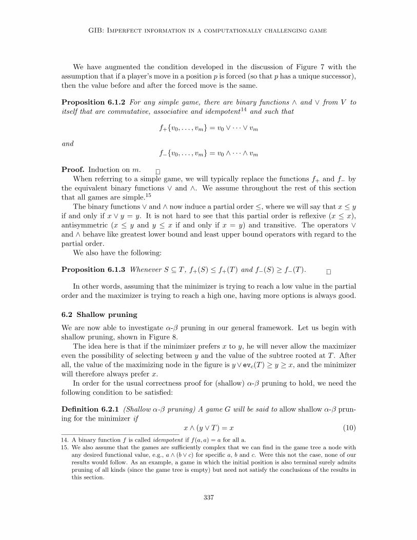
GIB: Imperfect information in a computationally challenging game
We have augmented the condition developed in the discussion of Figure 7 with theassumption that if a player’s move in a position p is forced (so that p has a unique successor),then the value before and after the forced move is the same.
Proposition 6.1.2 For any simple game, there are binary functions ∧ and ∨ from V toitself that are commutative, associative and idempotent14 and such that
f+{v0, . . . , vm} = v0 ∨ · · · ∨ vm
andf−{v0, . . . , vm} = v0 ∧ · · · ∧ vm
Proof. Induction on m.When referring to a simple game, we will typically replace the functions f+ and f− by
the equivalent binary functions ∨ and ∧. We assume throughout the rest of this sectionthat all games are simple.15
The binary functions ∨ and ∧ now induce a partial order ≤, where we will say that x ≤ yif and only if x ∨ y = y. It is not hard to see that this partial order is reflexive (x ≤ x),antisymmetric (x ≤ y and y ≤ x if and only if x = y) and transitive. The operators ∨and ∧ behave like greatest lower bound and least upper bound operators with regard to thepartial order.
We also have the following:
Proposition 6.1.3 Whenever S ⊆ T , f+(S) ≤ f+(T ) and f−(S) ≥ f−(T ).
In other words, assuming that the minimizer is trying to reach a low value in the partialorder and the maximizer is trying to reach a high one, having more options is always good.
6.2 Shallow pruning
We are now able to investigate α-β pruning in our general framework. Let us begin withshallow pruning, shown in Figure 8.
The idea here is that if the minimizer prefers x to y, he will never allow the maximizereven the possibility of selecting between y and the value of the subtree rooted at T . Afterall, the value of the maximizing node in the figure is y∨evc(T ) ≥ y ≥ x, and the minimizerwill therefore always prefer x.
In order for the usual correctness proof for (shallow) α-β pruning to hold, we need thefollowing condition to be satisfied:
Definition 6.2.1 (Shallow α-β pruning) A game G will be said to allow shallow α-β prun-ing for the minimizer if
x ∧ (y ∨ T ) = x (10)
14. A binary function f is called idempotent if f(a, a) = a for all a.15. We also assume that the games are sufficiently complex that we can find in the game tree a node with
any desired functional value, e.g., a ∧ (b ∨ c) for specific a, b and c. Were this not the case, none of ourresults would follow. As an example, a game in which the initial position is also terminal surely admitspruning of all kinds (since the game tree is empty) but need not satisfy the conclusions of the results inthis section.
337

Ginsberg
q q
q q
q
����AAAA
����SS
SS
CCCC
max
min
x
y T
Figure 8: T can be pruned (shallowly) if x ≤ y
for all x, y, T ∈ V with x ≤ y. The game will be said to allow shallow α-β pruning for themaximizer if
x ∨ (y ∧ T ) = x (11)
for all x, y, T ∈ V with x ≥ y. We will say that G allows shallow pruning if it allows shallowα-β pruning for both players.
The definition basically says that the backed up value at the root of the game tree isunchanged by pruning the maximizing subtree in the figure.
As we will see shortly, the expressions (10) and (11) describing shallow pruning areidentical to what are more typically known as absorption identities.
Definition 6.2.2 Suppose V is a set and ∧ and ∨ are two binary operators on V . Thetriple (V,∧,∨) is called a lattice if ∧ and ∨ are idempotent, commutative and associative,and satisfy the absorption identities in that for any x, y ∈ V ,
x ∨ (x ∧ y) = x (12)x ∧ (x ∨ y) = x (13)
We also have the following:
Definition 6.2.3 A lattice (V,∧,∨) is called distributive if ∧ and ∨ distribute with respectto one another, so that
x ∨ (y ∧ z) = (x ∨ y) ∧ (x ∨ z) (14)x ∧ (y ∨ z) = (x ∧ y) ∨ (x ∧ z) (15)
Lemma 6.2.4 Each of (12) and (13) implies the other. Each of (14) and (15) implies theother.
Proof. These are well known results from lattice theory (Gratzer, 1978).
Proposition 6.2.5 (Ginsberg & Jaffray, 2001) For a game G, the following conditionsare equivalent:
338
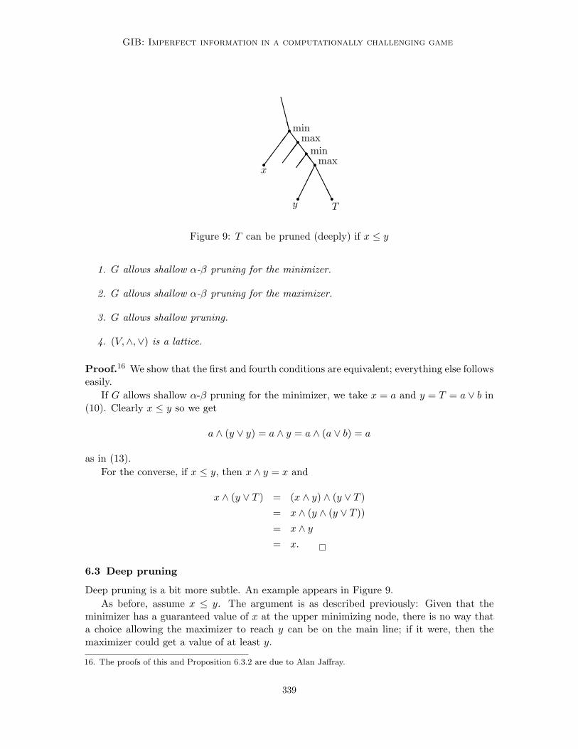
GIB: Imperfect information in a computationally challenging game
r r
r r
r
����AAAA
����SS
SS
CCCC
rmaxrmin
���
�� max
min
x
y T
Figure 9: T can be pruned (deeply) if x ≤ y
1. G allows shallow α-β pruning for the minimizer.
2. G allows shallow α-β pruning for the maximizer.
3. G allows shallow pruning.
4. (V,∧,∨) is a lattice.
Proof.16 We show that the first and fourth conditions are equivalent; everything else followseasily.
If G allows shallow α-β pruning for the minimizer, we take x = a and y = T = a ∨ b in(10). Clearly x ≤ y so we get
a ∧ (y ∨ y) = a ∧ y = a ∧ (a ∨ b) = a
as in (13).For the converse, if x ≤ y, then x ∧ y = x and
x ∧ (y ∨ T ) = (x ∧ y) ∧ (y ∨ T )= x ∧ (y ∧ (y ∨ T ))= x ∧ y
= x.
6.3 Deep pruning
Deep pruning is a bit more subtle. An example appears in Figure 9.As before, assume x ≤ y. The argument is as described previously: Given that the
minimizer has a guaranteed value of x at the upper minimizing node, there is no way thata choice allowing the maximizer to reach y can be on the main line; if it were, then themaximizer could get a value of at least y.
16. The proofs of this and Proposition 6.3.2 are due to Alan Jaffray.
339

Ginsberg
r
r
r
r
r
@@@@@@@@@
���
���
���
���
0
♣♦
♥♣
max
min
max
min
Figure 10: The deep pruning counterexample
Definition 6.3.1 (Deep α-β pruning) A game G will be said to allow α-β pruning for theminimizer if for any x, y, T, z1, . . . , z2i ∈ V with x ≤ y,
x ∧ (z1 ∨ (z2 ∧ · · · ∨ (z2i ∧ (y ∨ T ))) · · ·) =x ∧ (z1 ∨ (z2 ∧ · · · ∨ z2i) · · ·).
The game will be said to allow α-β pruning for the maximizer if
x ∨ (z1 ∧ (z2 ∨ · · · ∧ (z2i ∨ (y ∧ T ))) · · ·) =x ∨ (z1 ∧ (z2 ∨ · · · ∧ z2i) · · ·).
We will say that G allows pruning if it allows α-β pruning for both players.
As before, the prune allows us to remove the dominated node (y in Figure 9) and all of itssiblings.
The fact that a game allows shallow α-β pruning does not mean that it allows pruningin general, as is shown by the following counterexample. The example involves a game withone card that is known to both players; only the suit of the card matters. The game treeappears in Figure 10.
In this tree, a node labelled with a suit symbol is terminal and means that the maximizerwins if and only if the suit of the card matches the given symbol. So at the root of the giventree, the maximizer (whose turn it is to play) can choose to “turn over” the card, winningif and only if it’s a club, or can defer to the minimizer. The minimizer can choose to turnthe card (losing just in case it’s a diamond – the suit symbols refer to the maximizer’sresult), or hand the situation back to the maximizer. If the maximizer defers yet again,the minimizer can either turn over the card, losing if it’s a club, or simply declare victory(presumably his choice).
There is one other wrinkle in this game. At any point in the game, the maximizer canchange the card from either a diamond or a spade to a club.
Now let’s consider the game itself. At ply 4, the minimizer will obviously choose to winthe game. Thus at ply 3, the maximizer will need to choose ♥, winning just in case thecard is a heart. But this means that at ply 2, the minimizer will win the game, since if thecard is not a diamond he will move to the left (and win at once) while if the card is not aheart he can win by moving to the right. (Remember that the minimizer knows the suit
340

GIB: Imperfect information in a computationally challenging game
of the card.) The upshot of this is that the maximizer wins the overall game if and only ifthe card in question is a club. A formal analysis proceeds similarly, labelling the nodes asfollows:
r
r
r
r
r
@@@@@@@@@
���
���
���
���
0
♣♦
♥♣
♥ = ♥ ∨ 0
0 = ♣ ∧ 0
♣ = ♣ ∨ 0
0 = ♦ ∧♥
Note, incidentally, that the maximizer’s ability to change the card does not help him winthe game.
Now suppose that we apply deep pruning to this game. The ply four node is one wherethe minimizer can force a value of at most ♣, suggesting that the siblings of the bottom ♣node can be pruned. But doing so produces the following tree:
r
r
r
r
r
@@@@@@@@@
���
���
���
���
pruned?
♣♦
♥♣
1 = ♥ ∨♣♣
♣ ∨♦♦ = ♦ ∧ 1
If the maximizer reaches ply 3, he can win by changing the card to a club if need be.Of course, the minimizer won’t let the maximizer reach ply 3; at ply 2, he’ll move left
so that the maximizer wins only if the card is a diamond. That means that the maximizerwins at the root just in case the card is either a club or a diamond.
A partial graph of the values for this game is as follows:
r
r
r r r r������
QQQQQQ
����
AAAA������
����
0
1
♣ ♦♥ ♠
where we have included the crucial fact that x ∧ y = 0 if x 6= y (since the minimizer knowsthe card) and ♥ ∨ ♣ = 1 because the maximizer can invoke his special rule. Other leastupper bounds are not shown in the diagram. The maximizing function ∨ moves up thefigure; the minimizing function ∧ moves down.
The deep prune fails because we can’t “push” the value ♣ ∧ 0 past the ♥ to get to the♣ near the root. Somewhat more precisely, the problem is that
♥ = ♥ ∨ (♣ ∧ 0) 6= (♥ ∧♣) ∨ (♥ ∧ 0) = 0
This suggests the following:
341

Ginsberg
Proposition 6.3.2 (Ginsberg & Jaffray, 2001) For a game G, the following conditionsare equivalent:
1. G allows α-β pruning for the minimizer.
2. G allows α-β pruning for the maximizer.
3. G allows pruning.
4. (V,∧,∨) is a distributive lattice.
Proof. As before, we show only that the first and fourth conditions are equivalent. Sincepruning implies shallow pruning (take i = 0 in the definition), it follows that the firstcondition implies that (V,∧,∨) is a lattice.
From deep pruning for the minimizer with i = 1, we have that if x ≤ y, then for anyz1, z2, T ,
x ∧ (z1 ∨ (z2 ∧ (y ∨ T ))) = x ∧ (z1 ∨ z2)
Now take y = T = x to get
x ∧ (z1 ∨ (z2 ∧ x)) = x ∧ (z1 ∨ z2) (16)
It follows that each top level term in the left hand side of (16) is greater than or equal tothe right hand side; specifically
z1 ∨ (z2 ∧ x) ≥ x ∧ (z1 ∨ z2). (17)
We claim that this implies that the lattice in question is distributive.To see this, let u, v, w ∈ V . Now take z1 = u ∧ w, z2 = v and x = w in (17) to get
(u ∧ w) ∨ (v ∧ w) ≥ w ∧ ((u ∧ w) ∨ v) (18)
But v ∨ (u ∧ w) ≥ w ∧ (v ∨ u) is an instance of (17), and combining this with (18) gives us
(u ∧ w) ∨ (v ∧ w) ≥ w ∧ ((u ∧ w) ∨ v)≥ w ∧ w ∧ (v ∨ u)= w ∧ (v ∨ u)
This is the hard direction; w ∧ (v ∨ u) ≥ (u ∧ w) ∨ (v ∧ w) for any lattice becausew∧ (v∨u) ≥ u∧w and w∧ (v∨u) ≥ v∧w individually. Thus w∧ (v∨u) = (u∧w)∨ (v∧w),and deep pruning implies that the lattice is distributive.
For the converse, if the lattice is distributive and x ≤ y, then
x ∧ (z1 ∨ (z2 ∧ (y ∨ T ))) = (x ∧ z1) ∨ (x ∧ z2 ∧ (y ∨ T ))= (x ∧ z1) ∨ (x ∧ z2)= x ∧ (z1 ∨ z2)
where the second equality is a consequence of the fact that x ≤ (y∨T ), so that x = x∧(y∨T ).This validates pruning for i = 1; deeper cases are similar.
Finally, note that in games where this result applies, we can continue to use Algorithms2.2.5 or 2.3.3 without modification, since the prunes that they endorse continue to be soundas the game tree is expanded.
342

GIB: Imperfect information in a computationally challenging game
6.4 Application to imperfect information
In order to apply these ideas to games of imperfect information treated as in Section 5, weneed to show that the value set introduced there is a (hopefully distributive) lattice.
To do this, recall that there is redundant information in an arbitrary element F of 22S,
since if F contains both T and U with T ⊆ U (in other words, the maximizer can playfor either T or for U but U is properly better), the set T can be removed from F withoutaffecting the maximizer’s options in any interesting way. This suggests the following:
Definition 6.4.1 Let F ∈ 22Sfor an arbitrary set S. We will say that F is reduced if
there are no T,U ∈ F with T ⊆ U . We will say that F1 is a reduction of F2 if F1 is reducedand F1 ⊆ F2.
Lemma 6.4.2 Every F ∈ 22Shas a unique reduction.
Proof. This is immediate; just remove the subsumed elements from F . .We will denote the reduction of F by r(F).Armed with this definition, we can now modify Definition 5.0.6 in the obvious way,
replacing the value set V with the set of reduced elements of V and the maximizing andminimizing functions (8) and (9) with the reduced versions thereof, so that
max(F ,G) = r(F ∪ G) (19)
andmin({Fi}, {Gj}) = r({Fi ∩Gj}) (20)
Remember that we typically write ∨ for max and ∧ for min.
Proposition 6.4.3 Given the above definitions, (V,∨,∧) is a distributive lattice.
Proof. We need to show that max and min as defined above are commutative, associative,and idempotent, that they distribute with respect to one another, and that the absorptionidentity (12) is satisfied. Since the reduction operator clearly commutes with the initialdefinitions of max and min, commutativity, associativity and distributivity are obvious, asis the fact that ∨ is idempotent. To see that ∧ is idempotent, we have
F ∧ F = r({min(Fi, Fj)}) = r({Fi ∩ Fj})
but each element of the set on the righthand side is a subset of Fi ∩ Fi so
F ∧ F = r({Fi}) = r(F) = F .
For the absorption identity, we need to show that
F ∨ (F ∧ G) = F
ButF ∧ G = r{Fi ∩Gj}
343

Ginsberg
so
F ∨ (F ∧ G) = r(F ∨ r{Fi ∩Gj})= r({Fi} ∪ {Fi ∩Gj})= r({Fi})= r(F)= F
since, once again, each element of F ∧ G is subsumed by the corresponding Fi.It follows that an implementation designed to compute the value of an imperfect in-
formation game as described by Theorem 5.0.7 can indeed use α-β pruning to speed thecomputation.
6.5 Bridge implementation
Given this body of theory, we implemented a single-dummy version of gib’s double-dummysearch engine. Not surprisingly, the most difficult element of the implementation was build-ing efficient data structures for the manipulation of elements of 22S
.To handle this, we represented each element of S as a conjunction. We first identified
one of the two hidden hands H, and then for each card c, would write c if c were held byH and ¬c if c were not held by H. An element of 2S was then taken to be a disjunctivecombination of these conjunctions, and an element of 22S
was taken to be a list of suchdisjunctions. The advantage of this representation was that logical inference could be usedto construct the reduction of any such list.
In order to make this inference as efficient as possible, the disjunctions themselves wererepresented as binary decision diagrams, or bdd’s (Lind-Nielsen, 2000). There are a varietyof public domain implementations of bdd’s available, and we used one provided by Lind-Nielsen (Lind-Nielsen, 2000).17
The resulting implementation solves small endings (perhaps 16 cards left in total) quicklybut for larger endings, the running times come to be dominated by the bdd computations;this is hardly surprising, since the size of individual bdds can be exponential in the sizeof S (the number of possible distributions of the unseen cards). We found that we weregenerally able to solve 32-card endings in about a minute, but that the running times wereincreasing by two orders of magnitude as each additional card was added.
This is both good news and bad news. Viewed positively, the performance of the systemas constructed is far superior to the performance of preceding attempts to deal with theimperfect information arising in bridge. Frank et.al, for example, are only capable of solvingsingle suit combinations (13 cards left, give or take) using an algorithm that appears to takeseveral minutes to run (Frank, Basin, & Matsubara, 1998). They subsequently improve theperformance to an average time of 0.6 seconds (Frank et al., 2000), but are still restricted toproblems that are too small to be of much use to a program intended to play the completegame.
17. We tried a variety of non-bdd based implementations as well. The bdd-based implementation was farfaster than any of the others.
344
GIB: Imperfect information in a computationally challenging game
That’s the good news. The bad news is that a program capable only of solving an 8-card ending in a minute is inappropriate for production use. Gib is a production program,expected to play bridge at human speeds. Another approach was therefore needed.
7. Solving single-dummy problems in practice
7.1 Achievable sets
The key to practical application of the ideas in the previous section is the realization thatwhen it comes time to make a play, a single element of F must be selected: if you can playfor West to have the ♠Q or for each player to have three hearts but cannot cater to bothpossibilities simultaneously, you eventually have to actually make the choice.
Definition 7.1.1 Suppose that the value of the imperfect information game for G is F .Given a specific A ⊆ S, we will say that A is achievable if there is some F ∈ F for whichA ⊆ F .
In other words, the set A of situations is achievable if the maximizer has a plan that winsfor all elements of A.
Definition 7.1.2 Given a set S of situations, a payoff function for S is any functionf : 2S → IR such that f(U) ≤ f(T ) whenever U ⊆ T .
The payoff function evaluates potential achievable sets.
Definition 7.1.3 Let G be a game and S the associated set of situations. If f is a payofffunction for S, a solution to G under f is any achievable set A for which f(A) is maximal.
In practice, we need not find the actual value of the game; finding a solution to G underan appropriate payoff function suffices. In bridge, the payoff function is presumably theprobability that the cards are dealt as in the set A; this function clearly increases withincreasing set size as required by Definition 7.1.2 and can be evaluated in practice using theMonte Carlo sample of Section 3.
Instead of finding the solution to an imperfect information game, suppose instead thatwe have a Monte Carlo sample for the game consisting of a set of situations S = {si} thatis ordered as i = 0, . . . , n. We can now produce an achievable set A as follows:
Algorithm 7.1.4 To construct a maximal achievable set A from a sequence 〈s0, . . . , sn〉 ofsituations:
1. Set A = Ø.
2. For i = 0, . . . , n, if A ∪ {si} is achievable, set A = A ∪ {si}.
The algorithm constructs the achievable set in a greedy fashion, gradually adding elementsof S to A until no more can be added.
Definition 7.1.5 Given a game G and a sequence S of situations, the achievable set in-duced by S for G is the set constructed by Algorithm 7.1.4.
345

Ginsberg
From a computational point of view, the expensive step in the algorithm is determiningwhether or not the set A ∪ {si} is achievable. This is relatively straightforward, however,since the focus on a specific set effectively replaces the game G with a new game withvalues in {0, 1}. At any particular node n, if expanding n demonstrates that A ∪ {si} isnot achievable, the value of the game is zero. If expanding n indicates that A ∪ {si} isachievable once n is reached, then the value of the node n is one. Although the search spaceis unchanged from that of the original imperfect information game as in Definition 5.0.6,there is no longer any need to manipulate complex values, and the check for achievabilityis therefore tractable in practice.
Let me illustrate this by returning to our usual example of Section 5. Here is the fullyevaluated tree once again:
q q q q q q q q
q q q q
q q q q
q
�����������PPPPPPPPPPP����@@
@@
����
����
����
����A
AAA
AAAA
AAAA
AAAA
����
����C
CCC
CCCC
{S ∪ T}
{S, T}{S} {T} {S ∪ T}
{S} {T}{S ∪ T} {S} {T} {S ∪ T} {S ∪ T} {S ∪ T}
{S ∪ T} {S} {T} {S ∪ T}
Note that we have replaced the value at the root with its reduction.Now suppose that we view the set of positions as containing only two elements, s ∈ S
and t ∈ T . Presumably West holds the ♠Q in s, and East holds three hearts in t. If theordering chosen is 〈s, t〉, then we first try to achieve {s}. In this context, a node n is a winfor the maximizer if either the maximizer can indeed win at n or s is no longer possible (inwhich case the maximizer’s ability to achieve {s} is undiminished). The game tree becomes:
q q q q q q q q
q q q q
q q q q
q
�����������PPPPPPPPPPP����@@
@@
����
����
����
����A
AAA
AAAA
AAAA
AAAA
����
����C
CCC
CCCC
max
maxmin min min
min min1 1 0 1 1 1
1 1 0 1
S S S
S S
T T T
T T
All of the T branches are wins for the maximizer (who is concerned with s only), and theS branches are wins just in case the maximizer does indeed win (as he does if he guessesright at either of the first two plies). Backing up the values gives us:
346
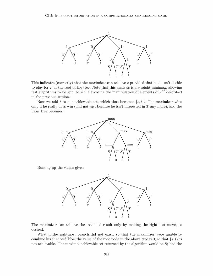
GIB: Imperfect information in a computationally challenging game
q q q q q q q q
q q q q
q q q q
q
�����������PPPPPPPPPPP����@@
@@
����
����
����
����A
AAA
AAAA
AAAA
AAAA
����
����C
CCC
CCCC
1
11 0 1
0 11 1 0 1 1 1
1 1 0 1
S S S
S S
T T T
T T
This indicates (correctly) that the maximizer can achieve s provided that he doesn’t decideto play for T at the root of the tree. Note that this analysis is a straight minimax, allowingfast algorithms to be applied while avoiding the manipulation of elements of 22S
describedin the previous section.
Now we add t to our achievable set, which thus becomes {s, t}. The maximizer winsonly if he really does win (and not just because he isn’t interested in T any more), and thebasic tree becomes:
q q q q q q q q
q q q q
q q q q
q
�����������PPPPPPPPPPP����@@
@@
����
����
����
����A
AAA
AAAA
AAAA
AAAA
����
����C
CCC
CCCC
max
maxmin min min
min min1 0 0 1 1 1
1 0 0 1
S S S
S S
T T T
T T
Backing up the values gives:
q q q q q q q q
q q q q
q q q q
q
�����������PPPPPPPPPPP����@@
@@
����
����
����
����A
AAA
AAAA
AAAA
AAAA
����
����C
CCC
CCCC
1
00 0 1
0 01 0 0 1 1 1
1 0 0 1
S S S
S S
T T T
T T
The maximizer can achieve the extended result only by making the rightmost move, asdesired.
What if the rightmost branch did not exist, so that the maximizer were unable tocombine his chances? Now the value of the root node in the above tree is 0, so that {s, t} isnot achievable. The maximal achievable set returned by the algorithm would be S; had the
347

Ginsberg
ordering been 〈t, s〉 instead, an alternative maximal achievable set of T would have beenreturned instead.
In any event, we have:
Proposition 7.1.6 Given a game G and a sequence S of situations, let A be the achievableset induced by S for G. Then no proper superset of A in S is achievable.
Proof. This is straightforward. For any element s ∈ S − A, we know that U ∪ {s} is notachievable for some U ⊆ A. Thus A ∪ {s} is not achievable as well.
Algorithm 7.1.4 allows us to construct maximal achievable sets relative to our MonteCarlo sample; recall that we are taking our sequence S of situations to be any orderingof the sample itself. In practice, however, it is important not to focus too sharply on thesample itself, lest the eventual achievable set constructed overfit irrelevant probabilisticcharacteristics of that sample. This can be accomplished by replacing the simple union instep 2 of the algorithm with some more complicated operation that captures the idea of“situations that are either like si or like those already in A.” In bridge, for example, A mightbe all situations where West has two or three hearts, and si might be some new situationwhere West has four hearts. The generalized union would be situations where West hastwo, three or four hearts. If this more general set is not achievable, another attempt couldbe made with the simple union. If we denote the “general union” by ⊕, Algorithm 7.1.4becomes:
Algorithm 7.1.7 To construct an achievable set A from a sequence 〈s0, . . . , sn〉 of situa-tions:
1. Set A = Ø.
2. For i = 0, . . . , n:
(a) If A⊕ {si} is achievable, set A = A⊕ {si}.(b) Otherwise, if A ∪ {si} is achievable, set A = A ∪ {si}.
This algorithm can be used in practice to find achievable sets that are either maximalor effectively so over the set of all possible instances, not just those appearing in the MonteCarlo sample.
7.2 Maximizing the payoff
It remains to find not just maximal achievable sets, but ones that approximate the solutionto the game in question given a particular payoff function.
To understand how we do this, let me draw an analogy between the problem we are tryingto solve and resource-constrained project scheduling (rcps). In rcps, one has a list of tasksto be performed, together with ordering constraints saying that certain tasks need to beperformed before others. In addition, each task uses a certain quantity of various resources;there are limitations on the availability of any particular resource at any particular time.As an example, building an aircraft wing may involve fabricating the top and bottom flightsurfaces, building the aileron, and attaching the two. It should be clear that the aileron
348

GIB: Imperfect information in a computationally challenging game
cannot be attached until both it and the wing have been constructed. Building each sectionmay involve the use of three sheetmetal workers, but only five may be available in general.
The goal in an rcps problem is typically to minimize the length of the schedule (oftencalled the makespan) without exceeding the resource limits. In building a wing, it is moreefficient (and more cost effective) to build it quickly than slowly.
Many production scheduling systems try to minimize makespan by building the schedulefrom the initial time forward. At each point, they select a task all of whose predecessorshave been scheduled, and then schedule that task as early as possible given the previouslyscheduled tasks and the resource constraints. Scheduling the tasks in this way produces alocally optimal schedule that may be improved by modifying the order in which the tasksare selected for scheduling.
One method for finding an appropriate modification to the selection order is known assqueaky wheel optimization, or swo (Joslin & Clements, 1999). In swo, a locally optimalschedule is examined to determine which tasks are scheduled most suboptimally relative tosome overall metric; those tasks are deemed to “squeak” and are then advanced in the tasklist so that they are scheduled earlier when the schedule is reconstructed. This process isrepeated, producing a variety of candidate solutions to the scheduling problem at hand; oneof these schedules is typically optimal or nearly so.
Applying swo to our game-playing problem is relatively straightforward.18 When weuse Algorithm 7.1.7 to construct an achievable set, we also construct as a byproduct a list ofsample elements to which that achievable set cannot be extended; moving elements of thislist forward in the sequence of 〈s0, . . . , sn〉 will cause them to be more likely to be includedin the achievable set A if the algorithm is reinvoked. The weights assigned to the failingsequence elements can be constructed by determining how representative each particularelement is of the remainder of the sample.
Returning to our example, suppose that the set S (where West has the ♠Q) has a singlerepresentative s1 in the Monte Carlo sample (presumably this means it is unlikely for Westto hold the card in question), while T has five such representatives t1, t2, t3, t4 and t5.Suppose also that the initial ordering of the six elements is 〈s1, t4, t2, t1, t5, t3〉.
Assuming that the maximizer loses his rightmost option (so that he cannot cater to Sand T simultaneously), the maximal achievable set corresponding to this ordering is S. Anexamination now reveals that all of the ti’s could have been achieved but weren’t; in swoterms, these elements of the sample “squeak.”
At the next iteration, the priorities of the ti’s are increased by moving them forward inthe sequence, while the priority of s1 falls. Perhaps the new ordering is 〈t4, t2, s1, t1, t5, t3〉.
This ordering can be easily seen to lead to the maximal achievable set T ; S ∪ T is stillunachievable. But the payoff assigned to T is likely to be much better than that assignedto S (a probability of 0.8 instead of 0.2, if the Monte Carlo sample itself is unweighted). Itis in this way that swo allows us to find a globally optimal (or nearly so) achievable set.
18. Squeaky wheel optimization was developed at the University of Oregon; the patent application for thetechnique has been allowed by the U.S. Patent and Trademark Office. The University’s interests in swoare licensed exclusively to On Time Systems, Inc. for use in scheduling and related applications, and toJust Write, Inc. for use in bridge-playing systems.
349

Ginsberg
7.3 Results
Our implementation of gib’s cardplay when declarer is based on the ideas described above.(As a defender, a direct Monte Carlo approach appears preferable because enough infor-mation is typically available about declarer’s hand to make the double-dummy assumptionreasonably valid.) The implementation is fast enough to conform to the time requirementsplaced on a production program (roughly one cpu minute to play each deal).
Evaluating the impact of these ideas on gib’s cardplay is difficult, since declarer play isalready the strongest aspect of its game. In extended matches between the two versions ofgib, the approach based on the ideas described here beats the Monte-Carlo based versionby approximately 0.1 imps/deal, but there is a great deal of noise in the data because mostof the swings correspond to differences in bidding or defensive play. It is possible to removesome of these differences artificially (requiring the bidding to be identical both times thedeal is played, for example), but defensive differences remain. Nevertheless, gib is currentlya strong enough player that the 0.1 imps/deal difference is significant.
The situation on problem deals, such as those from the par contests or from the Gitelmansets, is much clearer. In addition, many of the deals that gib gets “wrong” are in fact dealsthat gib plays correctly but that the problem composers play incorrectly (Gitelman or, inthe case of the par contests, Swiss bridge expert Pietro Bernasconi). In the following table,we have been generous with all parties, deeming a line to be correct if it is not clearlyinferior to another. Let me point out that the designers of the problems are attempting toconstruct deals where there is a unique solution (the “answer” to the test they are posingthe solver), so that a deal with multiple solutions is in fact one that the composer hasalready misanalyzed.
Source size BB GibMC GibSWO composer ambiguousBM level 1 36 16 31 36 35 0
level 2 36 8 23 34 34 1level 3 36 2 12 34 34 2level 4 36 1 21 31 34 4level 5 36 4 13 28 34 5
1998 par contest 12 0 5 11 12 21990 par contest 18 0 8 14 17 3
The rows are in order of increasing difficulty; it was universally felt among the humancompetitors that the deals in the 1990 par contest were far more difficult than those in1998. The columns are as follows:
Source is the source from which the problems were obtained.Size is the number of problems available from this particular source.BB gives the number of problems solved correctly by Bridge Baron 6.GibMC gives the number solved correctly by gib using a Monte Carlo approach.GibSWO gives the number solved correctly by gib using swo and achievable sets.composer gives the number solved correctly by the composer (in that the intended
solution was the best one available).ambiguous gives the number misanalyzed by the composer (in that multiple solutions
exist).
350

GIB: Imperfect information in a computationally challenging game
Note, incidentally, that gib’s performance is still less than perfect on these problems.The reason is that gib’s sample may be skewed in some way, or that swo may fail to finda global optimum among the set of possible achievable sets.
8. Conclusion
8.1 GIB compared
Other programs Gib participated in both the 1998 and the 2000 World ComputerBridge Championships. (There was no 1999 event.) Play was organized with each machineplaying two hands and the competitors being trusted not to cheat by “peeking” at partner’scards or those of the opponents.19
Each tournament began with a complete round robin among the programs, with the topfour programs continuing to a knockout phase. The matches in the round robin were quiteshort, and it was expected that bridge’s stochastic element would keep any program frombeing completely dominant.
While this may have been true in theory, in practice gib dominated both round robins,winning all of its matches in 1998 and all but one in 2000. The round robin results fromthe 2000 event were as follows:20
Gib WB Micro Buff Q-Plus Chip Baron M’lark TotalGib – 14 11 16 7 19 16 17 100WBridge 6 – 19 13 16 7 18 20 99Micro 9 1 – 18 15 15 13 20 91Buff 4 7 2 – 12 20 5 20 70Q-Plus 13 4 5 8 – 11 14 11 66Blue Chip 1 13 5 0 9 – 11 20 59Baron 4 2 7 15 6 9 – 14 57Meadowlark 3 0 0 0 9 0 6 – 18
Each match was converted first to imps and then to victory points, or VPs, with the twocompeting programs sharing the 20 VPs available in each match. The first entry in theabove table indicates that gib beat wbridge by 14 VPs to 6; the fourth that gib lostto q-plus bridge by 7 VPs to 13. (This is gib’s only loss ever to another program intournament play.)
In the 1998 knockout phase, gib beat Bridge Baron in the semifinals by 84 imps over 48deals. Had the programs been evenly matched, the imp difference could be expected to benormally distributed, and the observed 84 imp difference would be a 2.2 standard deviation
19. Starting with the 2001 event, each computer will handle only one of the four players, although thereis still no attempt to prevent the (networked) computers from transmitting illegal information betweenpartners.
20. There were eight competitors in the event: gib (www.gibware.com), Hans Leber’s q-plus(www.q-plus.com), Tomio and Yumiko Uchida’s micro bridge (www.threeweb.ad.jp/˜mcbridge),Mike Whittaker and Ian Trackman’s blue chip bridge (www.bluechipbridge.co.uk), Rod Lud-wig’s meadowlark bridge (rrnet.com/meadowlark), bridge baron (www.bridgebaron.com), andtwo newcomers: Doug Bannion’s bridge buff (www.bridgebuff.com) and Yves Costel’s wbridge(ourworld.compuserve.com/homepages/yvescostel).
351
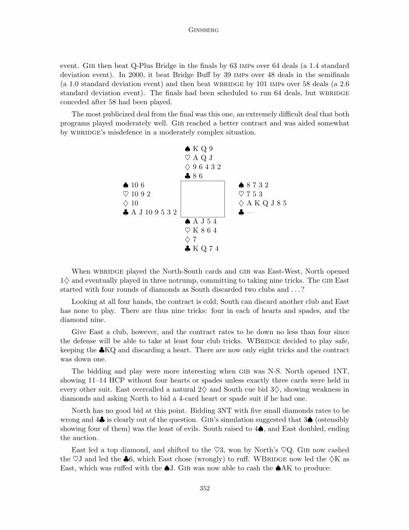
Ginsberg
event. Gib then beat Q-Plus Bridge in the finals by 63 imps over 64 deals (a 1.4 standarddeviation event). In 2000, it beat Bridge Buff by 39 imps over 48 deals in the semifinals(a 1.0 standard deviation event) and then beat wbridge by 101 imps over 58 deals (a 2.6standard deviation event). The finals had been scheduled to run 64 deals, but wbridgeconceded after 58 had been played.
The most publicized deal from the final was this one, an extremely difficult deal that bothprograms played moderately well. Gib reached a better contract and was aided somewhatby wbridge’s misdefence in a moderately complex situation.
♠ K Q 9♥ A Q J♦ 9 6 4 3 2♣ 8 6
♠ 10 6 ♠ 8 7 3 2♥ 10 9 2 ♥ 7 5 3♦ 10 ♦ A K Q J 8 5♣ A J 10 9 5 3 2 ♣ —
♠ A J 5 4♥ K 8 6 4♦ 7♣ K Q 7 4
When wbridge played the North-South cards and gib was East-West, North opened1♦ and eventually played in three notrump, committing to taking nine tricks. The gib Eaststarted with four rounds of diamonds as South discarded two clubs and . . . ?
Looking at all four hands, the contract is cold; South can discard another club and Easthas none to play. There are thus nine tricks: four in each of hearts and spades, and thediamond nine.
Give East a club, however, and the contract rates to be down no less than four sincethe defense will be able to take at least four club tricks. WBridge decided to play safe,keeping the ♣KQ and discarding a heart. There are now only eight tricks and the contractwas down one.
The bidding and play were more interesting when gib was N-S. North opened 1NT,showing 11–14 HCP without four hearts or spades unless exactly three cards were held inevery other suit. East overcalled a natural 2♦ and South cue bid 3♦, showing weakness indiamonds and asking North to bid a 4-card heart or spade suit if he had one.
North has no good bid at this point. Bidding 3NT with five small diamonds rates to bewrong and 4♣ is clearly out of the question. Gib’s simulation suggested that 3♠ (ostensiblyshowing four of them) was the least of evils. South raised to 4♠, and East doubled, endingthe auction.
East led a top diamond, and shifted to the ♥3, won by North’s ♥Q. Gib now cashedthe ♥J and led the ♣6, which East chose (wrongly) to ruff. WBridge now led the ♦K asEast, which was ruffed with the ♠J. Gib was now able to cash the ♠AK to produce:
352
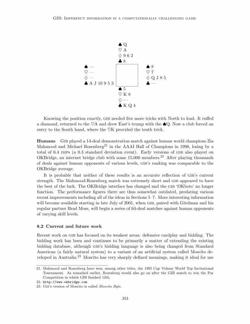
GIB: Imperfect information in a computationally challenging game
♠ Q♥ A♦ 9 6 2♣ 8
♠ — ♠ 8♥ — ♥ 7♦ — ♦ Q J 8 5♣ A J 10 9 5 3 ♣ —
♠ 5♥ K 8♦ —♣ K Q 4
Knowing the position exactly, gib needed five more tricks with North to lead. It ruffeda diamond, returned to the ♥A and drew East’s trump with the ♠Q. Now a club forced anentry to the South hand, where the ♥K provided the tenth trick.
Humans Gib played a 14-deal demonstration match against human world champions ZiaMahmood and Michael Rosenberg21 in the AAAI Hall of Champions in 1998, losing by atotal of 6.4 imps (a 0.3 standard deviation event). Early versions of gib also played onOKBridge, an internet bridge club with some 15,000 members.22 After playing thousandsof deals against human opponents of various levels, gib’s ranking was comparable to theOKBridge average.
It is probable that neither of these results is an accurate reflection of gib’s currentstrength. The Mahmood-Rosenberg match was extremely short and gib appeared to havethe best of the luck. The OKBridge interface has changed and the gib ‘OKbots’ no longerfunction. The performance figures there are thus somewhat outdated, predating variousrecent improvements including all of the ideas in Sections 5–7. More interesting informationwill become available starting in late July of 2001, when gib, paired with Gitelman and hisregular partner Brad Moss, will begin a series of 64-deal matches against human opponentsof varying skill levels.
8.2 Current and future work
Recent work on gib has focused on its weakest areas: defensive cardplay and bidding. Thebidding work has been and continues to be primarily a matter of extending the existingbidding database, although gib’s bidding language is also being changed from StandardAmerican (a fairly natural system) to a variant of an artificial system called Moscito de-veloped in Australia.23 Moscito has very sharply defined meanings, making it ideal for use
21. Mahmood and Rosenberg have won, among other titles, the 1995 Cap Volmac World Top InvitationalTournament. As remarked earlier, Rosenberg would also go on after the GIB match to win the ParCompetition in which GIB finished 12th.
22. http://www.okbridge.com
23. Gib’s version of Moscito is called Moscito Byte.
353

Ginsberg
by a computer program, and is an “action” system, working hard to make the opponents’bidding as difficult as possible.
With regard to defensive cardplay, the key elements of high level defense are to make ithard for partner to make a mistake while making it easy for declarer to do so. Providing gibwith these abilities will involve an extra level of recursion in the cardplay, as each elementof the Monte Carlo sample must now be considered from other players’ points of view, asthey generate and then analyze their own samples. These ideas have been implemented butcurrently lead to small performance degradations (approximately 0.05 imps/deal) becausethe computational cost of the recursive analyses require reducing the size of the MonteCarlo sample substantially. As processor speeds increase, it is reasonable to expect theseideas to bear significant fruit.
In 1997, Martel, a computer scientist himself, suggested that he expected gib to be thebest bridge player in the world in approximately 2003.† The work appears to be roughly onschedule.
8.3 Other games
I have left essentially untouched the question of to what extent the basic techniques we havediscussed could be applied to games of imperfect information other than bridge.
The ideas that we have presented are likely to be the most applicable in games wherethe perfect information variant is tractable but computationally challenging, and the as-sumption that one’s opponents are playing with perfect information is a reasonable one.This suggests that games like hearts and other trick-taking games will be amenable to ourtechniques, while games like poker (where it is essential to realize and exploit the fact thatthe opponents also have imperfect information) are likely to need other approaches.
Acknowledgments
A great many people have contributed to the gib project over the years. In the technicalcommunity, I would like to thank Jonathan Schaeffer, Rich Korf, David Etherington, BartMassey and the other members of cirl. In the bridge community, I have received invaluableassistance from Chip Martel, Rod Ludwig, Zia Mahmood, Andrew Robson, Alan Jaffray,Hans Kuijf, Fred Gitelman, Bob Hamman, Eric Rodwell, Jeff Goldsmith, Thomas Andrewsand the members of the rec.games.bridge community. The work itself has been supportedby Just Write, Inc., by DARPA/Rome Labs under contracts F30602-95-1-0023 and F30602-97-1-0294, and by the Boeing Company under contract AHQ569. To everyone who hascontributed, whether named above or not, I owe my deepest appreciation.
Appendix A. A summary of the rules of bridge
We give here a very brief summary of the rules of bridge. Readers wanting a more completedescription are referred to any of the many excellent texts available (Sheinwold, 1996).
Bridge is a card game for four players, who are split into two pairs. Members of a singlepair sit opposite one another, so that North-South form one pair and East-West the other.
354

GIB: Imperfect information in a computationally challenging game
The deck is distributed evenly among the players, so that each deal involves giving eachplayer a hand of 13 cards. The game then proceeds through a bidding and a playing phase.
The playing phase consists of 13 tricks, with each player contributing one card to eachtrick in a clockwise fashion. The player who plays first to any trick is said to lead to thattrick. The highest card of the suit led wins the trick (Ace is high and deuce low), unless atrump is played, in which case the highest trump wins the trick. The person who leads to atrick is free to lead any card he wishes; subsequent players must play a card of the suit ledif they have one, and can play any card they choose if they don’t. The winner of one trickleads to the next; the person who leads to the first trick (the opening leader) is determinedduring the bidding phase of the game.
The object of the card play phase is always for your partnership to take as many tricksas possible; there is no advantage to one partner’s taking a trick over another, and the orderin which the tricks are taken is irrelevant. After the opening leader plays the first card tothe first trick, the player to his left places his cards face up on the table so that all of theother players can see them. This player is called the dummy, and when it is dummy’s turnto play, dummy’s partner (who can see the partnership’s combined assets) selects the cardto be played. Dummy’s partner is called the declarer and the members of the other pairare called the defenders.
The purpose of the bidding phase is to identify trumps and the declarer, and also thecontract, which will be described shortly. The opening leader is identified as well, and isthe player to the declarer’s left.
During the bidding phase, various contracts are proposed. The dealer has the firstopportunity to propose a contract and subsequent opportunities are given to each playerin a clockwise direction. Each player has many opportunities to suggest a contract duringthis phase of the game, which is called the auction. Each partnership is required to explainthe meanings of their actions during the auction to the other side, if requested.
Each contract suggests a particular trump suit (or perhaps that there not be a trumpsuit at all). Each player suggesting a contract is committing his side to winning some par-ticular number of the 13 available tricks. The minimum commitment is 7 tricks, so thereare 35 possible contracts (each of 4 possible trumps, or no trumps, and seven possible com-mitments, from seven to thirteen tricks). These 35 contracts are ordered, which guaranteesthat the bidding phase will eventually terminate.
After the bidding phase is complete, the side that suggested the final contract is thedeclaring side. Of the two members of the declaring side, the one who first suggested theeventual trump suit (or no trumps) is the declarer. Play begins with the player to thedeclarer’s left leading to the first trick.
After the hand is complete, there are two possible outcomes. If the declaring side tookat least as many tricks as it committed to taking, the declaring side receives a positivescore and the defending side an equal but negative score. There are substantial bonusesawarded for committing to taking particular numbers of tricks; in general, the larger thecommitment, the larger the bonus. There are small bonuses awarded for winning tricksabove and beyond the commitment.
If the declaring side failed to honor its commitment, it receives a negative score andthe defenders receive an equal but positive score. The overall score in this case (where the
355

Ginsberg
declarer “goes down”) is generally smaller than the overall score in the case where declarer“makes it” (i.e., honors his commitment).
Appendix B. A new ending discovered by GIB
This deal occurred during a short imp match between gib and Bridge Baron.
♠ 9 6♥ Q J 8 5♦ A Q 3♣ K J 10 8
♠ K Q J 8 7 5 ♠ 4 3♥ 9 4 3 ♥ A 7 2♦ 7 ♦ J 10 6 2♣ 6 4 2 ♣ A Q 7 3
♠ A 10 2♥ K 10 6♦ K 9 8 5 4♣ 9 5
With South (gib) dealing at unfavorable vulnerability, the auction went P–2♠–X–P–3NT–all pass. (P is pass and X is double.) The opening lead was the ♠K, ducked by gib, andBridge Baron now switched to a small heart. East won the ace and returned to spades, gibwinning.
Gib cashed all the hearts, pitching a small club from its hand. It then tested thediamonds, learning of the bad break and winning the third diamond in hand. It then ledthe ♦9 in the following position:
♠ —♥ —♦ —♣ K J 10 8
♠ Q ♠ —♥ — ♥ —♦ — ♦ J♣ ? ? ? ♣ A ? ?
♠ 10♥ —♦ 9 8♣ 9
When gib pitched the ten of clubs from dummy (it had been aiming for this ending allalong), the defenders were helpless to take more than two tricks independent of the locationof the club queen. At the other table, Bridge Baron let gib play in 2♠ making exactly, andgib picked up 12 imps.
356

GIB: Imperfect information in a computationally challenging game
References
Adelson-Velskiy, G., Arlazarov, V., & Donskoy, M. (1975). Some methods of controlling thetree search in chess programs. Artificial Intelligence, 6, 361–371.
Bayardo, R. J., & Miranker, D. P. (1996). A complexity analysis of space-bounded learningalgorithms for the constraint satisfaction problem. In Proceedings of the ThirteenthNational Conference on Artificial Intelligence, pp. 298–304.
Billings, D., Papp, D., Schaeffer, J., & Szafron, D. (1998). Opponent modeling in poker. InProceedings of the Fifteenth National Conference on Artificial Intelligence, pp. 493–499.
Blackwood, E. (1979). Play of the Hand with Blackwood. Bobbs-Merrill.
Eskes, O. (1997). GIB: Sensational breakthrough in bridge software. IMP, 8 (2).
Frank, I. (1998). Search and Planning under Incomplete Information: A Study Using BridgeCard Play. Springer-Verlag, Berlin.
Frank, I., & Basin, D. (1998). Search in games with incomplete information: A case studyusing bridge card play. Artificial Intelligence, 100, 87–123.
Frank, I., Basin, D., & Bundy, A. (2000). Combining knowledge and search to solve single-suit bridge. In Proceedings of the Sixteenth National Conference on Artificial Intelli-gence, pp. 195–200.
Frank, I., Basin, D., & Matsubara, H. (1998). Finding optimal strategies for imperfectinformation games. In Proceedings of the Fifteenth National Conference on ArtificialIntelligence, pp. 500–507.
Ginsberg, M. L. (1993). Dynamic backtracking. Journal of Artificial Intelligence Research,1, 25–46.
Ginsberg, M. L., & Harvey, W. D. (1992). Iterative broadening. Artificial Intelligence, 55,367–383.
Ginsberg, M. L., & Jaffray, A. (2001). Alpha-beta pruning under partial orders. In Gamesof No Chance II. To appear.
Gratzer, G. (1978). General Lattice Theory. Birkhauser Verlag, Basel.
Greenblatt, R., Eastlake, D., & Crocker, S. (1967). The greenblatt chess program. In FallJoint Computer Conference 31, pp. 801–810.
Joslin, D. E., & Clements, D. P. (1999). Squeaky wheel optimization. Journal of ArtificialIntelligence Research, 10, 353–373.
Koller, D., & Pfeffer, A. (1995). Generating and solving imperfect information games. InProceedings of the Fourteenth International Joint Conference on Artificial Intelligence,pp. 1185–1192.
Levy, D. N. (1989). The million pound bridge program. In Levy, D., & Beal, D. (Eds.),Heuristic Programming in Artificial Intelligence, Asilomar, CA. Ellis Horwood.
Lind-Nielsen, J. (2000). BuDDy: Binary Decision Diagram package. Tech. rep., Depart-ment of Information Technology, Technical University of Denmark, DK-2800 Lyngby,Denmark.
357

Ginsberg
Lindelof, T. (1983). COBRA: The Computer-Designed Bidding System. Gollancz, London.
Marsland, T. A. (1986). A review of game-tree pruning. J. Intl. Computer Chess Assn.,9 (1), 3–19.
McAllester, D. A. (1988). Conspiracy numbers for min-max searching. Artificial Intelligence,35, 287–310.
Pearl, J. (1980). Asymptotic properties of minimax trees and game-searching procedures.Artificial Intelligence, 14 (2), 113–138.
Pearl, J. (1982). A solution for the branching factor of the alpha-beta pruning algorithmand its optimality. Comm. ACM, 25 (8), 559–564.
Plaat, A., Schaeffer, J., Pijls, W., & de Bruin, A. (1996). Exploiting graph properties of gametrees. In Proceedings of the Thirteenth National Conference on Artificial Intelligence,pp. 234–239.
Schaeffer, J. (1997). One Jump Ahead: Challenging Human Supremacy in Checkers.Springer-Verlag, New York.
Sheinwold, A. (1996). Five Weeks to Winning Bridge. Pocket Books.
Smith, S. J., Nau, D. S., & Throop, T. (1996). Total-order multi-agent task-network plan-ning for contract bridge. In Proceedings of the Thirteenth National Conference onArtificial Intelligence, Stanford, California.
Stallman, R. M., & Sussman, G. J. (1977). Forward reasoning and dependency-directedbacktracking in a system for computer-aided circuit analysis. Artificial Intelligence,9, 135–196.
Sterling, L., & Nygate, Y. (1990). PYTHON: An expert squeezer. J. Logic Programming,8, 21–40.
Wilkins, D. E. (1980). Using patterns and plans in chess. Artificial Intelligence, 14, 165–203.
358