Embed Size (px)
Citation preview
Geostatistical History Matching coupled with Adaptive Stochastic Sampling:
A zonation-based approach using Direct Sequential Simulation
Eduardo Barrela*
Instituto Superior Técnico, Av. Rovisco Pais 1, Lisboa 1049-001, Portugal
*E-mail address: [email protected]
A B S T R A C T
Advances in computing technology, over the past decades, allowed the development of a number of different History
Matching (HM) techniques. Nevertheless, the simultaneous integration of production data under geological consistency, as
part of the reservoir modelling workflow, still remains a challenge.
A geologically consistent approach aims to avoid solutions that are unrealistic under the reservoir’s general geological
characteristics. Unrealistic HM solutions often result in poor reservoir response forecasting. It is also essential to include
only geologically realistic models for uncertainty assessment based on multiple models that are consistent with the
geological data and also in order to match observed production history.
Geostatistical History Matching (GHM) can iteratively update static reservoir model properties through conditional
assimilation constrained to the production data, using geologically consistent perturbation. Multiple stochastic realizations
are assimilated following a zonation approach to account for the local match quality, providing a way to integrate
regionalized discretization of parameters with production data and engineering knowledge.
The present project proposes a new HM technique applied in uncertain reservoir conditions represented by geologically
consistent reservoir zonation, based on fault presence and production streamlines. The work explores the value of using a
geologically consistent zonation associated with production wells in GHM regions, coupled with adaptive stochastic
sampling and Bayesian inference for uncertainty quantification and optimization of geological and engineering properties.
This novel approach makes use of the Direct Sequential Simulation (DSS) algorithm for generation of stochastic realizations
and Particle Swarm Optimization (PSO) for parameter optimization. The approach is tested in a semi–synthetic case
study based on a braided–river depositional environment.
Keywords: History Matching, Geostatistics, Direct Sequential Simulation, Uncertainty Quantification, Particle Swarm
Optimization, Adaptive Stochastic Sampling.
1. Introduction
Reservoir modelling is a crucial step in the
development and management of petroleum
reservoirs. An accurate reservoir model is one that
honors all data at the scale and precision at which
they are available. Information available to model
the reservoir is continually updated over the course
of field development. Integration of static and
dynamic models is performed by modifying the static
model in order to match the observed historical
reservoir production data, using HM techniques.
However, the integration of both types of data into
reservoir modelling is a challenging task, as the
relationship between hard data and production data
is highly non-linear. The process of HM tries to
address this problem by applying changes to the
reservoir model in order to minimize a given cost
function, responsible for the quantification of the
mismatch between the observed production data
(historical data) and the dynamic model response
(simulated data). This introduces another problem
2
associated with HM. Multiple reservoir models
(static or dynamic) can produce equally matched
responses, making HM an ill-posed problem.
Over recent years, several approaches have been
developed to address History Matching of oil and gas
reservoirs. Methods depending on data assimilation,
like the Ensemble Kalman Filter (Evensen, et al.
2007), gradual deformation (Hu, et al. 2001),
probability perturbation (Caers & Hoffman, 2006) or
stochastic sequential simulation and co-simulation
(Mata-Lima, 2008), (Le Ravalec-Dupin & Da Veiga,
2011) have been proposed.
Other methods like Stochastic Optimisation
algorithms, allow reducing computational times by
sampling from the ensemble of best matched models
in order to improve matches. Algorithms such as the
Neighbourhood Algorithm (Sambridge, 1999), the
Genetic Algorithm (Erbas & Christie, 2007), the
Particle Swarm Optimisation (Mohamed, 2011) and
Differential Evolution (Hajidazeh, et al. 2009) have
been developed on recent years. By sampling only for
the models that fit better according to the
evolutionary principle, adaptive stochastic
optimisation allows a reduction in computational
costs.
The present project proposes a new HM
technique, coupling Traditional GHM methodologies
with the integration of Adaptive Stochastic
Sampling. The proposed methodology applies a
GHM technique under uncertain reservoir conditions
represented by geologically consistent reservoir
zonation, based on fault presence and fluid
production streamlines. The work explores the value
of using a geologically consistent zonation
methodology, associated with production wells in
Geostatistical History Matched regions, coupled with
adaptive stochastic sampling and Bayesian inference
for uncertainty quantification and optimization of
geological and engineering properties.
This novel approach makes use of the Direct
Sequential Simulation (DSS) (Soares, 2001)
algorithm for generation of stochastic realizations
and Particle Swarm Optimization (PSO) (Kennedy
& Eberhart, 1995) for parameter optimization. The
approach is tested in a semi–synthetic case study
based on a braided–river depositional environment.
2. Methodology Workflow
Following the works on regionalization–based
HM algorithms done by Hoffman & Caers (2005) and
Mata–Lima (2008), the proposed methodology
couples adaptive stochastic sampling with Zonation–
Based GHM. The proposed methodology is
synthetized by the following workflow:
First step (Zonation-Based GHM; Fig. 1):
1. Regionalization of the reservoir area
according to a given fault model and area of influence
of the wells, resulting in a cube with a zone being
assigned for each well or for a group of wells.
2. Simulation of a set of permeability (�) and
porosity (�) realizations through DSS, honouring the
well data, histograms and spatial distribution
revealed by the variogram;
3. Evaluation of the dynamic responses for
each of the realizations and calculation of the
mismatch between the simulated response and real
production data, using an objective function;
4. Calculation of a correlation coefficient
between each dynamic response and generation of a
cube composed of different correlation coefficients
per zone;
5. Creation of a composite cube of � and �,
with each region being populated by the
corresponding realization with the lowest mismatch,
calculated in step 3;
6. Return to step 2, using Co–DSS and the
cubes calculated in steps 4 and 5 as local correlation
coefficient and soft data, respectively. The algorithm
is expected to run up to a maximum number of
iterations, or until a pre–defined mismatch value is
reached.
3
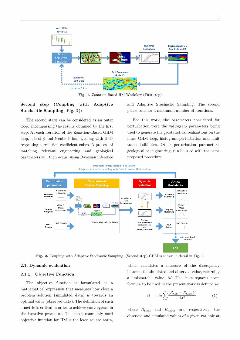
Fig. 1. Zonation-Based HM Workflow (First step)
Second step (Coupling with Adaptive
Stochastic Sampling; Fig. 2):
The second stage can be considered as an outer
loop, encompassing the results obtained by the first
step. At each iteration of the Zonation–Based GHM
loop, a best � and � cube is found, along with their
respecting correlation coefficient cubes. A process of
matching relevant engineering and geological
parameters will then occur, using Bayesian inference
and Adaptive Stochastic Sampling. The second
phase runs for a maximum number of iterations.
For this work, the parameters considered for
perturbation were the variogram parameters being
used to generate the geostatistical realizations on the
inner GHM loop, histogram perturbation and fault
transmissibilities. Other perturbation parameters,
geological or engineering, can be used with the same
proposed procedure.
Fig. 2. Coupling with Adaptive Stochastic Sampling. (Second step) GHM is shown in detail in Fig. 1.
2.1. Dynamic evaluation
2.1.1. Objective Function
The objective function is formulated as a
mathematical expression that measures how close a
problem solution (simulated data) is towards an
optimal value (observed data). The definition of such
a metric is critical in order to achieve convergence in
the iterative procedure. The most commonly used
objective function for HM is the least square norm,
which calculates a measure of the discrepancy
between the simulated and observed value, returning
a “mismatch” value, � . The least squares norm
formula to be used in the present work is defined as:
� = � ∑( �,��� − �,���)22�2
�
�=� (1)
where �,��� and �,��� are, respectively, the
observed and simulated values of a given variable at
4
timestep �. �2 is the error, or standard deviation,
associated to the measurement of a the same variable
at the same timestep.
2.1.2. Correlation coefficient
Due to the importance of the correlation
coefficient in the proposed GHM workflow, it is
crucial to make sure its value mimics the misfit value
obtained by the objective function. Meaning, a
process that integrates calculations of misfit and
correlation coefficients should guarantee that when
calculated, these values change symmetrically and in
the same proportion, under different configurations
of observation data curves. This issue was also
tackled, within the scope of this work, with the
development of a new approach to calculate a
correlation coefficient based on the misfit value. The
following step–by–step list describes the calculation
of the correlation coefficient being used by the GHM
algorithm.
1. For all timesteps and for the production variable to be matched, calculate a response difference, and the
corresponding error, respectively ∆��� and ∆�����, according to the following:
∆��� = ∣ (�,���) − (�,���)∣ (2)
∆�����= ��2 − ∆��� (3)
2. Calculate the final deviation towards observed data for a given timestep, ∆��� , according to:
∆���= { �,��� − (∆��� + ∆�����) " �,��� ≥ ∆��� + ∆����� 0 " �,��� < ∆��� + ∆�����
(4)
3. Normalization of the value obtained in step 2 according to the following:
&� =
⎩{⎨{⎧1 − ∆���(∆��� + ∆����� + ∆���) " ∆��� ≤ ∆����� + ∆���
0 " ∆��� > ∆����� + ∆���
(5)
4. The final correlation coefficient & for a given response is obtained by:
& = ∑ &�/�=11 (6)
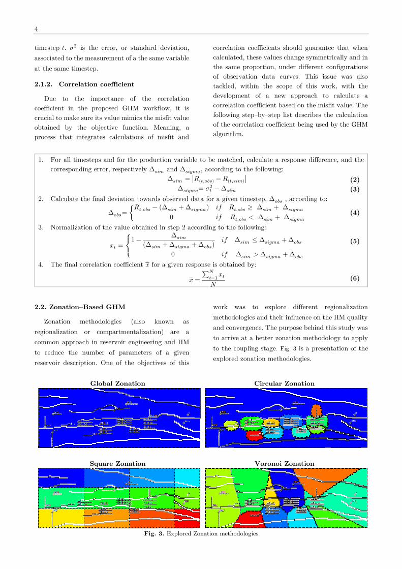
2.2. Zonation–Based GHM
Zonation methodologies (also known as
regionalization or compartmentalization) are a
common approach in reservoir engineering and HM
to reduce the number of parameters of a given
reservoir description. One of the objectives of this
work was to explore different regionalization
methodologies and their influence on the HM quality
and convergence. The purpose behind this study was
to arrive at a better zonation methodology to apply
to the coupling stage. Fig. 3 is a presentation of the
explored zonation methodologies.
Global Zonation Circular Zonation
Square Zonation Voronoi Zonation
Fig. 3. Explored Zonation methodologies
5
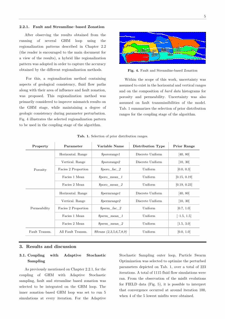
2.2.1. Fault and Streamline–based Zonation
After observing the results obtained from the
running of several GHM loop using the
regionalization patterns described in Chapter 2.2
(the reader is encouraged to the main document for
a view of the results), a hybrid like regionalization
pattern was adopted in order to capture the accuracy
obtained by the different regionalization methods.
For this, a regionalization method containing
aspects of geological consistency, fluid flow paths
along with their area of influence and fault zonation,
was proposed. This regionalization method was
primarily considered to improve mismatch results on
the GHM stage, while maintaining a degree of
geologic consistency during parameter perturbation.
Fig. 4 illustrates the selected regionalization pattern
to be used in the coupling stage of the algorithm.
Fig. 4. Fault and Streamline-based Zonation
Within the scope of this work, uncertainty was
assumed to exist in the horizontal and vertical ranges
and on the composition of hard data histograms for
porosity and permeability. Uncertainty was also
assumed on fault transmissibilities of the model.
Tab. 1 summarizes the selection of prior distribution
ranges for the coupling stage of the algorithm.
Tab. 1. Selection of prior distribution ranges.
Property Parameter Variable Name Distribution Type Prior Range
Porosity
Horizontal. Range $pororange1 Discrete Uniform [40, 80]
Vertical. Range $pororange2 Discrete Uniform [10, 30]
Facies 2 Proportion $poro_fac_2 Uniform [0.0, 0.3]
Facies 1 Mean $poro_mean_1 Uniform [0.15, 0.19]
Facies 2 Mean $poro_mean_2 Uniform [0.19, 0.23]
Permeability
Horizontal. Range $permrange1 Discrete Uniform [40, 80]
Vertical. Range $permrange2 Discrete Uniform [10, 30]
Facies 2 Proportion $perm_fac_2 Uniform [0.7, 1.0]
Facies 1 Mean $perm_mean_1 Uniform [–1.5, 1.5]
Facies 2 Mean $perm_mean_2 Uniform [1.5, 3.0]
Fault Transm. All Fault Transm. $ftrans (2,3,5,6,7,8,9) Uniform [0.0, 1.0]
3. Results and discussion
3.1. Coupling with Adaptive Stochastic
Sampling
As previously mentioned on Chapter 2.2.1, for the
coupling of GHM with Adaptive Stochastic
sampling, fault and streamline based zonation was
selected to be integrated on the GHM loop. The
inner zonation–based GHM loop was set to run 5
simulations at every iteration. For the Adaptive
Stochastic Sampling outer loop, Particle Swarm
Optimization was selected to optimize the perturbed
parameters depicted on Tab. 1, over a total of 223
iterations. A total of 1115 fluid flow simulations were
ran. From the observation of the misfit evolutions
for FIELD data (Fig. 5), it is possible to interpret
that convergence occurred at around iteration 100,
when 4 of the 5 lowest misfits were obtained.
6
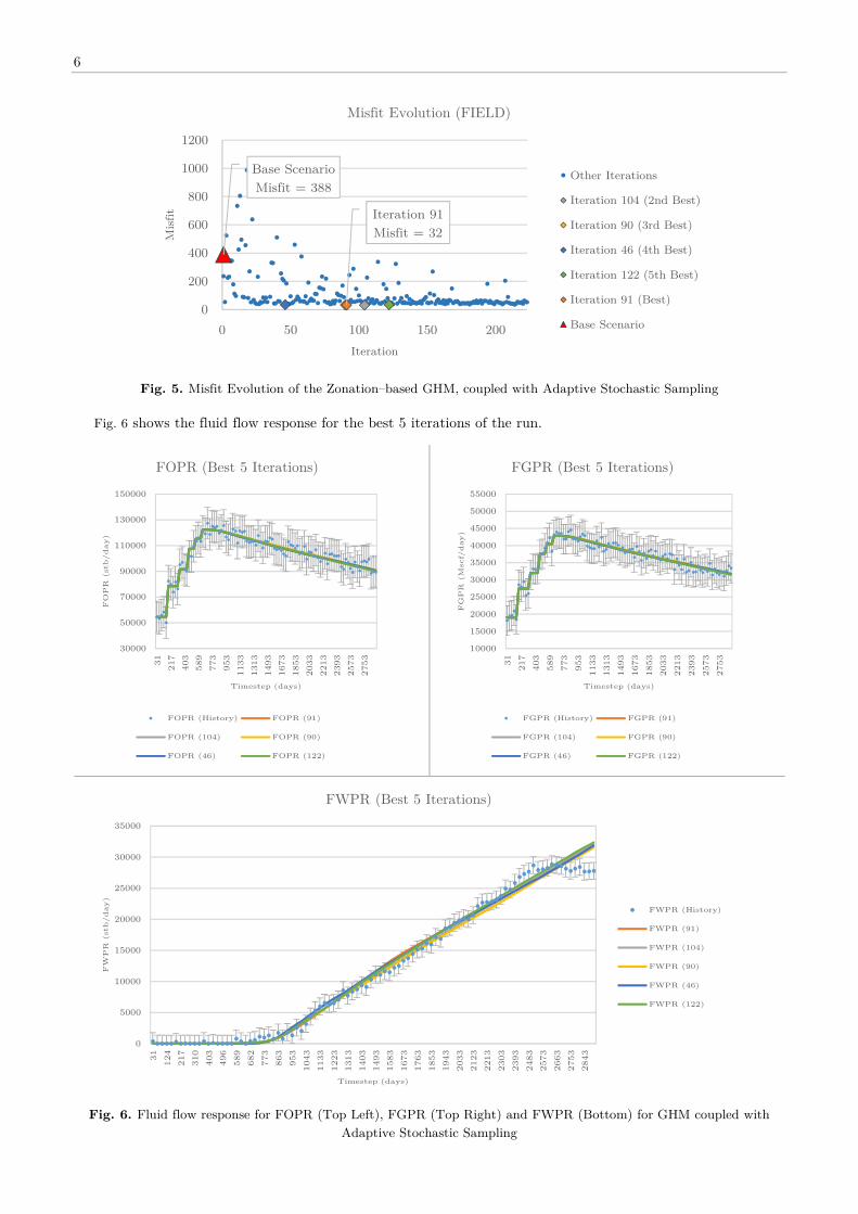
Fig. 5. Misfit Evolution of the Zonation–based GHM, coupled with Adaptive Stochastic Sampling
Fig. 6 shows the fluid flow response for the best 5 iterations of the run.
Fig. 6. Fluid flow response for FOPR (Top Left), FGPR (Top Right) and FWPR (Bottom) for GHM coupled with
Adaptive Stochastic Sampling
Iteration 91
Misfit = 32
Base Scenario
Misfit = 388
0
200
400
600
800
1000
1200
0 50 100 150 200
Misfit
Iteration
Misfit Evolution (FIELD)
Other Iterations
Iteration 104 (2nd Best)
Iteration 90 (3rd Best)
Iteration 46 (4th Best)
Iteration 122 (5th Best)
Iteration 91 (Best)
Base Scenario
30000
50000
70000
90000
110000
130000
150000
31
21
7
40
3
58
9
77
3
95
3
11
33
13
13
14
93
16
73
18
53
20
33
22
13
23
93
25
73
27
53
FO
PR
(stb/day)
Timestep (days)
FOPR (Best 5 Iterations)
FOPR (History) FOPR (91)
FOPR (104) FOPR (90)
FOPR (46) FOPR (122)
10000
15000
20000
25000
30000
35000
40000
45000
50000
55000
31
21
7
40
3
58
9
77
3
95
3
11
33
13
13
14
93
16
73
18
53
20
33
22
13
23
93
25
73
27
53
FG
PR
(M
scf/
day)
Timestep (days)
FGPR (Best 5 Iterations)
FGPR (History) FGPR (91)
FGPR (104) FGPR (90)
FGPR (46) FGPR (122)
0
5000
10000
15000
20000
25000
30000
35000
31
12
4
21
7
31
0
40
3
49
6
58
9
68
2
77
3
86
3
95
3
10
43
11
33
12
23
13
13
14
03
14
93
15
83
16
73
17
63
18
53
19
43
20
33
21
23
22
13
23
03
23
93
24
83
25
73
26
63
27
53
28
43
FW
PR
(stb/day)
Timestep (days)
FWPR (Best 5 Iterations)
FWPR (History)
FWPR (91)
FWPR (104)
FWPR (90)
FWPR (46)
FWPR (122)

7
Fig. 7 shows the Parameter vs Misfit plots for the
perturbation of fault transmissibilities. On some of
the parameters, a dispersion of values can be
observed, along the lower values of misfit. However,
it is possible to interpret the concentration of most
frequent parameter values for lower misfit iterations,
namely on faults 3, 5, 6, with remaining fault
transmissibility values being too sparse to assign a
specific interval with a degree of confidence.
$ftrans2 $ftrans3 $ftrans5
$ftrans6
$ftrans7 $ftrans8 $ftrans9
Fig. 7. Fault Transmissibility parameter value (y axis) vs Misfit (x axis)
Fig. 8 shows the concentration of parameter
values for horizontal and vertical permeability
ranges over the course of the iterations. A
concentration of lower values for horizontal
permeability ranges ($permrange1) is observed,
while for vertical ranges, the spread of parameter
values, within the assumed prior range,
corresponding to lower misfits, is much higher.
$permrange1 $permrange2
Fig. 8. Permeability Range vs Misfit (Left – Horizontal Range, Right – Vertical range)
0.0
0.2
0.4
0.6
0.8
1.0
0
20
40
60
80
10
0
0.0
0.2
0.4
0.6
0.8
1.0
0
20
40
60
80
10
0
0.0
0.2
0.4
0.6
0.8
1.0
0
20
40
60
80
10
0
0.0
0.2
0.4
0.6
0.8
1.0
0
20
40
60
80
10
0
0.0
0.2
0.4
0.6
0.8
1.0
0 20 40 60 80 100
0.0
0.2
0.4
0.6
0.8
1.0
0
20
40
60
80
10
0
0.0
0.2
0.4
0.6
0.8
1.0
0
20
40
60
80
10
0
40
50
60
70
80
0
20
40
60
80
100
Horizo
ntal Range
Misfit
10
15
20
25
30
0
20
40
60
80
100
Vertica
l Range
Misfit
8
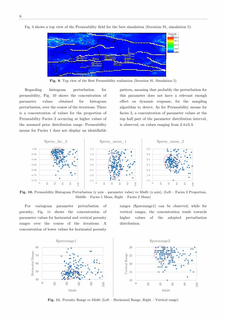
Fig. 9 shows a top view of the Permeability field for the best simulation (Iteration 91, simulation 5).
Fig. 9. Top view of the Best Permeability realization (Iteration 91, Simulation 5)
Regarding histogram perturbation for
permeability, Fig. 10 shows the concentration of
parameter values obtained for histogram
perturbation, over the course of the iterations. There
is a concentration of values for the proportion of
Permeability Facies 2 occurring at higher values of
the assumed prior distribution range. Permeability
means for Facies 1 does not display an identifiable
pattern, meaning that probably the perturbation for
this parameter does not have a relevant enough
effect on dynamic response, for the sampling
algorithm to detect. As for Permeability means for
facies 2, a concentration of parameter values at the
top half part of the parameter distribution interval,
is observed, on values ranging from 2.4±0.3.
$perm_fac_2 $perm_mean_1 $perm_mean_2
Fig. 10. Permeability Histogram Perturbation (y axis – parameter value) vs Misfit (x axis), (Left – Facies 2 Proportion,
Middle – Facies 1 Mean, Right – Facies 2 Mean)
For variogram parameter perturbation of
porosity, Fig. 11 shows the concentration of
parameter values for horizontal and vertical porosity
ranges over the course of the iterations. A
concentration of lower values for horizontal porosity
ranges ($pororange1) can be observed, while for
vertical ranges, the concentration tends towards
higher values of the adopted perturbation
distribution.
$pororange1 $pororange2
Fig. 11. Porosity Range vs Misfit (Left – Horizontal Range, Right – Vertical range)
0.70
0.75
0.80
0.85
0.90
0.95
1.00
0
20
40
60
80
10
0
-1.5
-1.0
-0.5
0.0
0.5
1.0
1.5
0
20
40
60
80
10
0
1.5
1.8
2.0
2.3
2.5
2.8
3.0
0
20
40
60
80
10
0
40
50
60
70
80
0
20
40
60
80
100
Horizo
ntal Range
Misfit
10
15
20
25
30
0
20
40
60
80
100
Vertica
l Range
Misfit
9
Fig. 12 shows a top view of the Permeability field for the best simulation (Iteration 91, Simulation 5).
Fig. 12. Top view of the Best Porosity realization (Iteration 91, Simulation 5)
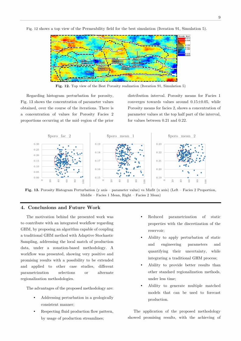
Regarding histogram perturbation for porosity,
Fig. 13 shows the concentration of parameter values
obtained, over the course of the iterations. There is
a concentration of values for Porosity Facies 2
proportions occurring at the mid–region of the prior
distribution interval. Porosity means for Facies 1
converges towards values around 0.15±0.05, while
Porosity means for facies 2, shows a concentration of
parameter values at the top half part of the interval,
for values between 0.21 and 0.22.
$poro_fac_2 $poro_mean_1 $poro_mean_2
Fig. 13. Porosity Histogram Perturbation (y axis – parameter value) vs Misfit (x axis) (Left – Facies 2 Proportion,
Middle – Facies 1 Mean, Right – Facies 2 Mean)
4. Conclusions and Future Work
The motivation behind the presented work was
to contribute with an integrated workflow regarding
GHM, by proposing an algorithm capable of coupling
a traditional GHM method with Adaptive Stochastic
Sampling, addressing the local match of production
data, under a zonation-based methodology. A
workflow was presented, showing very positive and
promising results with a possibility to be extended
and applied to other case studies, different
parametrization selections or alternate
regionalization methodologies.
The advantages of the proposed methodology are:
• Addressing perturbation in a geologically
consistent manner;
• Respecting fluid production flow pattern,
by usage of production streamlines;
• Reduced parametrization of static
properties with the discretization of the
reservoir;
• Ability to apply perturbation of static
and engineering parameters and
quantifying their uncertainty, while
integrating a traditional GHM process;
• Ability to provide better results than
other standard regionalization methods,
under less time;
• Ability to generate multiple matched
models that can be used to forecast
production.
The application of the proposed methodology
showed promising results, with the achieving of
0.00
0.05
0.10
0.15
0.20
0.25
0.30
0
20
40
60
80
10
0
0.15
0.16
0.17
0.18
0.19
0
20
40
60
80
10
0
0.19
0.20
0.21
0.22
0.23
0
20
40
60
80
10
0

10
multiple History Matched models with considerably
low misfits (lowest misfit of 32, on a 96 timestep
run). The creation of an ensemble of multiple history
matched models by solving the ill–posed calibration
problem, allows the prediction of reservoir behavior
with a degree of uncertainty. Nevertheless, a
limitation of the proposed methodology is its
dependency on the right choice of prior ranges, which
is essential for good optimization results.
The successful application of the proposed
methodology to a challenging semi-synthetic
reservoir case study delivers good perspectives for its
application to real cases. Further research on this
area could be focused towards performing forecasting
using the proposed methodology, applying other
types of parameter perturbation, alternate methods
of reservoir zonation, integration of the methodology
with facies perturbation or seismic inversion.
References
Caers, J., & Hoffman, T. (2006). The probability perturbation method: A new look at Bayesian inverse modeling.
Mathematical geology, 38(1), 81-100.
Erbas, D., & Christie, M. A. (2007). Effect of sampling strategies on prediction uncertainty estimation. In SPE
Reservoir Simulation Symposium. Society of Petroleum Engineers.
Evensen, G., Hove, J., Meisingset, H., & Reiso, E. (2007). Using the EnKF for assisted history matching of a
North Sea reservoir model. SPE Reservoir Simulation Symposium. Society of Petroleum Engineers.
Hajizadeh, Y., Christie, M. A., & Demyanov, V. (2009). Application of differential evolution as a new method for
automatic history matching. Kuwait International Petroleum Conference and Exhibition. Society of
Petroleum Engineers.
Hoffman, B. T., & Caers, J. (2005). Regional probability perturbations for history matching. Journal of Petroleum
Science and Engineering, 46(1), 53-71.
Hu, L. Y., Blanc, G., & Noetinger, B. (2001). Gradual deformation and iterative calibration of sequential
stochastic simulations. Mathematical Geology, 33(4), 475-489.
Kennedy, J., & Eberhart, R. C. (1995). Particle swarm optimization. Proceedings of IEEE International
Conference on Neural Networks. Piscataway, NJ.
Le Ravalec-Dupin , M., & Da Veiga, S. (2011). Cosimulation as a perturbation method for calibrating porosity
and permeability fields to dynamic data. Computers & geosciences, 37(9), 1400-1412.
Mata-Lima, H. (2008). Reservoir characterization with iterative direct sequential co-simulation: integrating fluid
dynamic data into stochastic model. 62(3), 59-72.
Mohamed, L. (2011). Novel sampling techniques for reservoir history matching optimisation and uncertainty
quantification in flow prediction. PhD Thesis Institute of Petroleum Engineering, Heriot-Watt University,
Edinburgh, UK.
Sambridge, M. (1999). Geophysical inversion with a neighbourhood algorithm—II. Appraising the ensemble.
Geophysical Journal International, 138(3), 727-746.
Soares, A. (2001). Direct sequential simulation and cosimulation. Mathematical Geology, 33 (8), 911–926.