EFFICIENT SAMPLING IN STOCHASTIC BIOLOGICAL

MODELS

by

Rory Donovan-Maiye

M.S., University of Washington, 2005

B.A., Reed College, 2004

Submitted to the Graduate Faculty of

the Department of Computational Biology in partial fulfillment

of the requirements for the degree of

Doctor of Philosophy

University of Pittsburgh

2016

UNIVERSITY OF PITTSBURGH

SCHOOL OF MEDICINE

This dissertation was presented

by

Rory Donovan-Maiye

It was defended on

May 31, 2016

and approved by

Daniel Zuckerman, Department of Computational and Systems Biology

James Faeder, Department of Computational and Systems Biology

Jeremy Berg, Department of Computational and Systems Biology

Christopher Langmead, Computational Biology Department, CMU

John Woolford, Biology Department, CMU

Dissertation Director: Daniel Zuckerman, Department of Computational and Systems Biology

ii

EFFICIENT SAMPLING IN STOCHASTIC BIOLOGICAL MODELS

Rory Donovan-Maiye, PhD

University of Pittsburgh, 2016

Even when the underlying dynamics are known, studying the emergent behavior of stochastic

biological systems in silico can be computationally intractable, due to the difficulty of compre-

hensively sampling these models. This thesis presents the study of two techniques for efficiently

sampling models of complex biological systems. First, the weighted ensemble enhanced sampling

technique is adapted for use in sampling chemical kinetics simulations, as well as spatially re-

solved stochastic reaction-diffusion kinetics. The technique is shown to scale to large, cell-scale

simulations, and to accelerate the sampling of observables by orders of magnitude in some cases.

Second, I study the free energy estimates of peptides and proteins using Markov random fields.

These graphical models are constructed from physics-based forcefields, uniformly sampled at dif-

ferent densities in dihedral angle space, and free energy estimates are computed using loopy belief

propagation. The effect of sample density on the free energy estimates provided by loopy belief

propagation is assessed, and it is found that in most cases a modest increase in sample density

leads to significant improvement in convergence. Additionally, the approximate free energies from

loopy belief propagation are compared to statistically exact computations and are confirmed to be

both accurate and orders of magnitude faster than traditional methods in the models assessed.

iii

TABLE OF CONTENTS

1.0 INTRODUCTION . . . . . . . . . . . . . . . . . . . . . . . . . . . . . . . . . . . . 1

1.1 Weighted Ensemble in Non-Spatial Systems . . . . . . . . . . . . . . . . . . . . 1

1.2 Weighted ensemble in spatial systems . . . . . . . . . . . . . . . . . . . . . . . . 5

1.3 Studying the Effects of Sampling Density in Graphical Models of Peptides and

Proteins . . . . . . . . . . . . . . . . . . . . . . . . . . . . . . . . . . . . . . . 7

1.3.1 Introduction to discrete Markov random fields . . . . . . . . . . . . . . . . 9

2.0 WEIGHTED ENSEMBLE IN NON-SPATIAL SYSTEMS . . . . . . . . . . . . . . 14

2.1 Introduction . . . . . . . . . . . . . . . . . . . . . . . . . . . . . . . . . . . . . 14

2.2 Methodology . . . . . . . . . . . . . . . . . . . . . . . . . . . . . . . . . . . . . 15

2.2.1 Stochastic Chemical Kinetics & BioNetGen . . . . . . . . . . . . . . . . . 15

2.2.2 Weighted Ensemble (WE) . . . . . . . . . . . . . . . . . . . . . . . . . . 16

2.2.2.1 Basic WE: Probability Distribution Evolving in Time . . . . . . . 18

2.2.2.2 Steady-State . . . . . . . . . . . . . . . . . . . . . . . . . . . . . 18

2.2.3 Estimation of Computational Efficiency . . . . . . . . . . . . . . . . . . . 20

2.2.4 Limitations of Our Implementation . . . . . . . . . . . . . . . . . . . . . 21

2.3 Models & Results . . . . . . . . . . . . . . . . . . . . . . . . . . . . . . . . . . 21

2.3.1 Enzymatic Futile Cycle . . . . . . . . . . . . . . . . . . . . . . . . . . . . 22

2.3.1.1 Model . . . . . . . . . . . . . . . . . . . . . . . . . . . . . . . . 22

2.3.1.2 WE Parameters . . . . . . . . . . . . . . . . . . . . . . . . . . . 22

2.3.1.3 Results . . . . . . . . . . . . . . . . . . . . . . . . . . . . . . . 23

2.3.2 Schlögl Reactions . . . . . . . . . . . . . . . . . . . . . . . . . . . . . . . 25

2.3.2.1 Model . . . . . . . . . . . . . . . . . . . . . . . . . . . . . . . . 25

iv

2.3.2.2 WE Parameters . . . . . . . . . . . . . . . . . . . . . . . . . . . 26

2.3.2.3 Results . . . . . . . . . . . . . . . . . . . . . . . . . . . . . . . 26

2.3.3 Yeast Polarization . . . . . . . . . . . . . . . . . . . . . . . . . . . . . . . 29

2.3.3.1 Model . . . . . . . . . . . . . . . . . . . . . . . . . . . . . . . . 30

2.3.3.2 WE Parameters . . . . . . . . . . . . . . . . . . . . . . . . . . . 30

2.3.3.3 Results . . . . . . . . . . . . . . . . . . . . . . . . . . . . . . . 30

2.3.4 Epigenetic Switch . . . . . . . . . . . . . . . . . . . . . . . . . . . . . . . 31

2.3.4.1 Model . . . . . . . . . . . . . . . . . . . . . . . . . . . . . . . . 31

2.3.4.2 WE Parameters . . . . . . . . . . . . . . . . . . . . . . . . . . . 32

2.3.4.3 Results . . . . . . . . . . . . . . . . . . . . . . . . . . . . . . . 32

2.3.5 FcεRI-Mediated Signaling . . . . . . . . . . . . . . . . . . . . . . . . . . 33

2.3.5.1 Model . . . . . . . . . . . . . . . . . . . . . . . . . . . . . . . . 33

2.3.5.2 WE Parameters . . . . . . . . . . . . . . . . . . . . . . . . . . . 35

2.3.5.3 Results . . . . . . . . . . . . . . . . . . . . . . . . . . . . . . . 35

2.4 Discussion . . . . . . . . . . . . . . . . . . . . . . . . . . . . . . . . . . . . . . 35

2.4.1 Strengths of WE . . . . . . . . . . . . . . . . . . . . . . . . . . . . . . . 37

2.4.2 Comparison to Other Approaches . . . . . . . . . . . . . . . . . . . . . . 37

2.4.3 Future Applications . . . . . . . . . . . . . . . . . . . . . . . . . . . . . . 39

2.5 Acknowledgments . . . . . . . . . . . . . . . . . . . . . . . . . . . . . . . . . . 40

3.0 WEIGHTED ENSEMBLE IN SPATIAL SYSTEMS . . . . . . . . . . . . . . . . . 41

3.1 Introduction . . . . . . . . . . . . . . . . . . . . . . . . . . . . . . . . . . . . . 41

3.2 Methods . . . . . . . . . . . . . . . . . . . . . . . . . . . . . . . . . . . . . . . 43

3.2.1 Weighted Ensemble . . . . . . . . . . . . . . . . . . . . . . . . . . . . . . 43

3.2.2 Kinetic Monte Carlo for spatial behavior of biochemically active species:

MCell . . . . . . . . . . . . . . . . . . . . . . . . . . . . . . . . . . . . . 49

3.2.3 Complex model construction: CellOrganizer and BioNetGen . . . . . . . . 50

3.3 Models . . . . . . . . . . . . . . . . . . . . . . . . . . . . . . . . . . . . . . . . 51

3.3.1 Toy Diffusive Binding Model . . . . . . . . . . . . . . . . . . . . . . . . . 53

3.3.2 Complex Model in Realistic Cellular Geometry . . . . . . . . . . . . . . . 53

3.3.3 Neuromuscular Junction . . . . . . . . . . . . . . . . . . . . . . . . . . . 57

v

3.4 Results . . . . . . . . . . . . . . . . . . . . . . . . . . . . . . . . . . . . . . . . 59

3.4.1 Toy Diffusive Binding Model . . . . . . . . . . . . . . . . . . . . . . . . . 59

3.4.2 Cross-Compartmental Signaling Network in a Realistic Cell Geometry . . . 62

3.4.3 Time Dependent Kinetics: Neuromuscular Junction . . . . . . . . . . . . . 64

3.5 Discussion . . . . . . . . . . . . . . . . . . . . . . . . . . . . . . . . . . . . . . 69

3.5.1 Strengths and Weaknesses of WE . . . . . . . . . . . . . . . . . . . . . . 69

3.5.2 Summary and Outlook . . . . . . . . . . . . . . . . . . . . . . . . . . . . 71

3.6 Supporting Information . . . . . . . . . . . . . . . . . . . . . . . . . . . . . . . 71

4.0 GRAPHICAL MODEL FREE ENERGIES OF PEPTIDES AND PROTEINS . . . 72

4.1 Introduction . . . . . . . . . . . . . . . . . . . . . . . . . . . . . . . . . . . . . 72

4.2 Overview of Graph Generation . . . . . . . . . . . . . . . . . . . . . . . . . . . 74

4.2.1 Choosing Edges . . . . . . . . . . . . . . . . . . . . . . . . . . . . . . . . 74

4.2.2 Node States from Dihedral Degrees of Freedom . . . . . . . . . . . . . . . 76

4.2.3 Node and Edge Potentials . . . . . . . . . . . . . . . . . . . . . . . . . . 77

4.3 Overview of Free Energy Calculations of Graphs . . . . . . . . . . . . . . . . . . 78

4.3.1 Brute-Force . . . . . . . . . . . . . . . . . . . . . . . . . . . . . . . . . . 78

4.3.2 Polymer Growth . . . . . . . . . . . . . . . . . . . . . . . . . . . . . . . 79

4.3.3 Belief Propagation . . . . . . . . . . . . . . . . . . . . . . . . . . . . . . 81

4.3.3.1 Message Passing . . . . . . . . . . . . . . . . . . . . . . . . . . 81

4.3.3.2 Computing Final Beliefs . . . . . . . . . . . . . . . . . . . . . . 83

4.3.3.3 Computing Free Energies from Beliefs . . . . . . . . . . . . . . . 83

4.4 Interactive Graph Visualization . . . . . . . . . . . . . . . . . . . . . . . . . . . 85

4.5 Implementation Details . . . . . . . . . . . . . . . . . . . . . . . . . . . . . . . 85

4.6 Systems and Results . . . . . . . . . . . . . . . . . . . . . . . . . . . . . . . . . 87

4.6.1 Agreement of Belief Propagation, Polymer Growth, and Brute-Force Free

Energies in a Simple Molecular System . . . . . . . . . . . . . . . . . . . 87

4.6.2 Determining Adequate Sampling Density in a Small Test System . . . . . . 90

4.6.3 Exploring Sampling Density in Larger Test Systems . . . . . . . . . . . . 92

4.6.4 Comparing belief propagation free energies to statistically exact estimates

in the binding pocket of a Protein: T4 Lysozyme Mutant . . . . . . . . . . 98

vi

4.6.4.1 Results for Artificial “Binding Pocket” Peptide . . . . . . . . . . 98

4.6.4.2 Results for Lysozyme . . . . . . . . . . . . . . . . . . . . . . . . 100

4.6.4.3 ∆F for a Lysozyme Mutant . . . . . . . . . . . . . . . . . . . . . 104

4.6.5 Future Work . . . . . . . . . . . . . . . . . . . . . . . . . . . . . . . . . . 106

4.7 Summary . . . . . . . . . . . . . . . . . . . . . . . . . . . . . . . . . . . . . . . 107

5.0 CONCLUSIONS . . . . . . . . . . . . . . . . . . . . . . . . . . . . . . . . . . . . . 109

APPENDIX A. CORRECTING FOR DISCRETIZATION IN PARTITION FUNC-

TION ESTIMATES . . . . . . . . . . . . . . . . . . . . . . . . . . . . . . . . . . . 111

A.1 Deriving the Exact Formula for Entropy . . . . . . . . . . . . . . . . . . . . . . 111

A.2 Discretizing the Exact Entropy Formula . . . . . . . . . . . . . . . . . . . . . . 113

A.3 Corrections for Z and F, but not E . . . . . . . . . . . . . . . . . . . . . . . . . 114

APPENDIX B. UNIFORM SAMPLING COMPUTES THE CORRECT PARTITION

FUNCTION . . . . . . . . . . . . . . . . . . . . . . . . . . . . . . . . . . . . . . . . 117

APPENDIX C. CODE EXCERPTS . . . . . . . . . . . . . . . . . . . . . . . . . . . . . 119

BIBLIOGRAPHY . . . . . . . . . . . . . . . . . . . . . . . . . . . . . . . . . . . . . . . 122

vii

LIST OF FIGURES

1 Weighted Ensemble Schematic Description . . . . . . . . . . . . . . . . . . . . . . 3

2 The Schlögl reactions . . . . . . . . . . . . . . . . . . . . . . . . . . . . . . . . . 5

3 Toy MCell Model . . . . . . . . . . . . . . . . . . . . . . . . . . . . . . . . . . . 6

4 Example Markov Random Field . . . . . . . . . . . . . . . . . . . . . . . . . . . . 10

5 Ising Model . . . . . . . . . . . . . . . . . . . . . . . . . . . . . . . . . . . . . . 11

6 More Complicated Graphs for Pairwise Markov Random Fields . . . . . . . . . . . 13

7 Enzymatic Futile Cycle PDF . . . . . . . . . . . . . . . . . . . . . . . . . . . . . . 24

8 Schlögl Reactions PDF . . . . . . . . . . . . . . . . . . . . . . . . . . . . . . . . 28

9 Schlögl Reactions Flux . . . . . . . . . . . . . . . . . . . . . . . . . . . . . . . . 29

10 Epigenetic Switch Flux . . . . . . . . . . . . . . . . . . . . . . . . . . . . . . . . 34

11 FcεRI-Mediated Signaling PDF . . . . . . . . . . . . . . . . . . . . . . . . . . . . 36

12 Distribution of Sampling Power . . . . . . . . . . . . . . . . . . . . . . . . . . . . 46

13 Software Pipeline for Realistic Cell Geometry Simulations . . . . . . . . . . . . . . 52

14 Toy Model Geometry . . . . . . . . . . . . . . . . . . . . . . . . . . . . . . . . . 54

15 Cellular Geometry . . . . . . . . . . . . . . . . . . . . . . . . . . . . . . . . . . . 55

16 Signal Transduction Network . . . . . . . . . . . . . . . . . . . . . . . . . . . . . 56

17 Frog Neuromuscular Junction Model Schematic . . . . . . . . . . . . . . . . . . . 57

18 Sampling Rare States of the Toy Binding Model . . . . . . . . . . . . . . . . . . . 61

19 Accelerated Sampling of High P2 Levels . . . . . . . . . . . . . . . . . . . . . . . 63

20 Steady-State Estimate of Time to Produce Five P2 . . . . . . . . . . . . . . . . . . 65

21 Enhanced Sampling of the First Fusion Time Distribution in the NMJ Model in Low

Calcium Conditions . . . . . . . . . . . . . . . . . . . . . . . . . . . . . . . . . . 67

viii

22 Verification of Empirical Fusion Rate Law Extended to Low Calcium Regime . . . 68

23 Outline of graph construction and use . . . . . . . . . . . . . . . . . . . . . . . . . 75

24 Polymer Growth Schematic . . . . . . . . . . . . . . . . . . . . . . . . . . . . . . 80

25 MRF Visualization Tool . . . . . . . . . . . . . . . . . . . . . . . . . . . . . . . . 86

26 Thr-4 Polymer Growth Free Energy . . . . . . . . . . . . . . . . . . . . . . . . . . 89

27 Thr-4 Free Energy Convergence . . . . . . . . . . . . . . . . . . . . . . . . . . . . 91

28 Alanine-4/8 Entropy and Average Energy at Different Sample Sizes . . . . . . . . . 93

29 Threonine-4/8 Entropy and Average Energy at Different Sample Sizes . . . . . . . . 94

30 Valine-4/8 Entropy and Average Energy at Different Sample Sizes . . . . . . . . . . 95

31 Leucine-4/8 Entropy and Average Energy at Different Sample Sizes . . . . . . . . . 96

32 Phenylalanine-4/8 Entropy and Average Energy at Different Sample Sizes . . . . . . 97

33 Peptide Structure . . . . . . . . . . . . . . . . . . . . . . . . . . . . . . . . . . . . 99

34 Peptide Free Energy Estimates . . . . . . . . . . . . . . . . . . . . . . . . . . . . . 101

35 Lysozyme Structure . . . . . . . . . . . . . . . . . . . . . . . . . . . . . . . . . . 102

36 Binding Pocket Free Energy Estimates . . . . . . . . . . . . . . . . . . . . . . . . 103

37 Mutational energy and Entropy differences . . . . . . . . . . . . . . . . . . . . . . 105

ix

1.0 INTRODUCTION

A common dilemma one faces in constructing computational models of biological systems is a

trade-off between model complexity and the tractability of simulating or sampling said model.

While there is merit in keeping models as simple as possible, when one is interested in studying

multi-scale behavior in complex systems, it is not always obvious which model ingredients are es-

sential and which are superfluous. As data accumulation accelerates, model ingredients proliferate,

and larger, more complete models of biological systems become possible to construct at multiple

scales, it behooves us to concern ourselves with how to sample ever larger models.

This dissertation focusses on this question in two different settings: the cellular scale and the

molecular scale. In the first chapter I study how the weighted ensemble methodology can accelerate

the sampling of rare events in stochastic chemical kinetics models. In the second chapter I examine

how the same formalism can aid in sampling spatially resolved cellular simulations. The third

chapter departs from the cellular scale to focus on molecular systems, and there I examine how

sampling density affects the accuracy of loopy belief propagation free energy estimates of peptides

and proteins.

1.1 WEIGHTED ENSEMBLE IN NON-SPATIAL SYSTEMS

My coworkers and I applied the “weighted ensemble” resampling technique to stochastic chemi-

cal kinetics systems biology models. Using the weighted ensemble framework, we were able to

observe rare events with orders of magnitude greater precision than a brute-force approach, and

were able to out-preform the state of the art technique (wSSA) on models of anything greater than

trivial complexity [1].

1

Stochastic behavior is an essential facet of biological processes such as mRNA expression,

protein expression, and epigenetic processes [2, 3, 4, 5, 6, 7, 8, 9, 10, 11, 12, 13, 14, 15]. Stochas-

tic chemical kinetics simulations are often used to study systems biology models of such pro-

cesses [16, 17, 18]. One of the more common stochastic approaches, and the one employed in

the present study, is the stochastic simulation algorithm (SSA), also known as the Gillespie algo-

rithm [19, 20, 16].

As stochastic systems biology models approach the true complexity of the systems being mod-

eled, it quickly becomes intractable to investigate rare behaviors using naïve (“brute-force”) simu-

lation approaches. By their very nature, rare events occur infrequently; confoundingly, rare events

are often those of most interest. For example, the switching of a bistable system from one state

to another may happen so infrequently that running a stochastic simulation long enough to see

transitions is (extremely) computationally prohibitive [21]. This impediment only grows as model

complexity increases, and as such it poses a serious hurdle for systems models as they grow more

intricate.

Several approaches to speeding up the simulation of rare events in stochastic chemical kinetic

systems exist. A variety of “leaping” methods can, by taking advantage of approximate time-

scale separation, accelerate the SSA itself [22, 23, 24, 25, 26, 27, 28, 29]. Kuwahara and Mura’s

weighted stochastic simulation (wSSA) method [30] was refined by Gillespie and Petzold et al. [31,

32, 33, 34], and is based on importance sampling. The forward flux sampling method of ten Wolde

et al. [21, 35, 36, 37] uses a series of interfaces in state-space to reduce computational effort, as

does the non-equilibrium umbrella sampling approach [38, 39].

Rare event sampling is also an active topic in the field of molecular dynamics simulations,

and many approaches have been proposed. Of the approaches that do not irreversibly modify the

free energy landscape of the system, some notable methods include dynamic importance sam-

pling [40], milestoning [41], transition path sampling [42], transition interface sampling [43], for-

ward flux sampling [37], non-equilibrium umbrella sampling [39], and weighted ensemble sam-

pling [44, 45, 46, 47, 48, 49, 50, 51]. For a summary of these methods, see [52]. Many of the ideas

behind these techniques are not exclusive to molecular dynamics simulations, and can be adapted

to studying stochastic chemical kinetic models. For example, dynamic importance sampling seems

to be closely related to wSSA.

2

t = 0 t = τ t = 2τ t = 3τ

U(x)

bin 1 bin 2 bin 3

U(x)

bin 1 bin 2 bin 3

U(x)

bin 1 bin 2 bin 3

U(x)

bin 1 bin 2 bin 3

U(x)

bin 1 bin 2 bin 3

U(x)

bin 1 bin 2 bin 3

U(x)

bin 1 bin 2 bin 3

U(x)

bin 1 bin 2 bin 3

Probability:1/2 1/4 1/81 1/16

WE

Dynami

cs WE

Dynami

cs WE

Dynami

cs WE

x x x x

x x x x

Time Propagation: Arbitrary Dynamics Engine

Split

ting/

Mer

ging

: Wei

ghte

d En

sem

ble

Figure 1: Weighted ensemble (WE) simulation depicted for a configuration/state-space divided

into bins. Multiple trajectories are run using any dynamics software (here we use the SSA in

BioNetGen) and checked every τ for bin location. Trajectories are assigned weights (symbols –

see legend) that sum to one and are split and combined according to statistical rules that preserve

unbiased kinetic behavior.

3

Because of its relative simplicity of implementation, and promise for sampling rare events, we

applied one of these methods, the weighted ensemble algorithm (WE) to well-established model

systems of stochastic kinetic chemical reactions. These models range in complexity from one

species and two reactions, to 354 species and 3680 reactions. For the systems studied, WE proves

many orders of magnitude faster than SSA simulation alone, offers linear parallel scaling, returns

full distributions of desired species at arbitrary times, and can yield mean first passage times (MF-

PTs) via the setup of a feedback steady-state.

WE’s strategy of statistical natural selection or statistical ratcheting is schematized in Fig. 1.

First, the space is divided/classified into non-overlapping “bins” which are typically static, al-

though dynamic and adaptive tessellations are possible [46]. A target number of trajectories, Mtarg,

is set for each bin. Multiple trajectories are initiated and each is assigned a weight so that the sum

of weights is one. Trajectories are then simulated independently according to the desired dynam-

ics (e.g., molecular dynamics or SSA) and checked intermittently (every τ units of time) for their

location. If a trajectory of weight w is found to occupy a previously unoccupied bin, that trajectory

is replicated to obtain the target number of copies, Mtarg, for the bin. Daughter trajectories’ weights

are set to w/Mtarg, to sum to the weight of the parent trajectory. If a bin is occupied by more than the

target number, trajectories must be pruned in a statistical fashion maintaining the sum of weights.

Specifically, the two lowest weight trajectories are “merged” by randomly selecting one of them

to survive, with probability proportional to their weights, and the surviving trajectory absorbs the

weight of the pruned one. This process is repeated as needed, and maintains an exact statistical

representation of the evolving distribution of trajectories [46].

In particular, we applied the weighted ensemble (WE) [44, 45, 46, 47, 48, 49, 50, 51] approach

to systems-biology models of stochastic chemical kinetics equations, implemented in BioNet-

Gen [18, 53]. Increases in computational efficiency on the order of 1020 were attained for a simple

system of biological relevance (the enzymatic futile cycle), and on the order of 1012 for a large

systems-biology model (FcεRI), with 354 species and 3680 reactions. An example of our results

is illustrated in Fig. 8.

The weighted ensemble approach is easy to understand and implement, statistically exact [46],

and easy to parallelize. It can yield long-timescale information such as mean first passage times

(MFPTs) from simulations of much shorter length, and offers perfect (linear) parallel scaling. It

4

A + 2Xk1�*)�k2

3X

Bk3�*)�k4

X

k1 = 3 ⇥ 10�7

k2 = 10�4

k3 = 10�3

k4 = 3.5

A = 105

B = 2 ⇥ 105

(a)

ÈÈÈÈÈ

ÈÈ

È

ÈÈÈ

ÈÈÈÈÈÈÈÈÈÈÈÈÈÈÈÈÈÈÈÈÈÈÈÈÈÈÈÈÈÈÈÈÈÈÈÈÈÈÈÈÈÈÈÈÈÈÈÈÈÈÈÈÈÈÈÈÈÈÈÈÈÈÈÈÈÈÈÈÈÈÈÈÈÈÈÈÈÈÈÈÈÈÈÈÈÈÈÈÈÈÈÈÈÈÈÈÈÈÈÈÈÈÈÈÈÈÈÈÈÈÈÈÈÈÈÈÈÈÈÈÈÈÈÈÈÈÈÈÈÈÈÈÈÈÈÈÈÈÈÈÈÈÈÈÈÈÈÈÈÈÈÈÈÈÈÈÈÈÈÈÈÈÈÈÈÈÈÈÈÈÈÈÈÈÈÈÈÈÈÈÈÈÈÈÈÈÈÈÈÈÈÈÈÈÈÈÈÈÈÈÈÈÈÈÈÈÈÈÈÈÈÈÈÈÈÈÈÈÈÈÈÈÈÈÈÈÈÈÈÈÈÈÈÈÈÈÈÈÈÈÈÈÈÈÈÈÈÈÈÈÈÈÈÈÈÈÈÈÈÈÈÈÈÈÈÈÈÈÈÈÈÈÈÈÈÈÈÈÈÈÈÈÈÈÈÈÈÈÈÈÈÈÈÈÈÈÈÈÈÈÈÈÈÈÈÈÈÈÈÈÈÈÈÈÈÈÈÈÈÈÈÈÈÈÈÈÈÈÈÈÈÈÈÈÈÈÈÈÈÈÈÈÈÈÈÈÈÈÈÈÈÈÈÈÈÈÈÈÈÈÈÈÈÈÈÈÈÈÈÈÈÈÈÈÈÈÈÈÈÈÈÈÈÈÈÈÈÈÈÈÈÈÈÈÈÈÈÈÈÈÈÈÈÈÈÈÈÈÈÈÈÈÈÈÈÈÈÈÈÈÈÈÈÈÈÈÈÈÈÈÈÈÈÈÈÈÈÈÈÈÈÈÈÈÈÈÈÈÈÈÈÈÈÈÈÈÈÈÈÈÈÈÈÈÈÈÈÈÈÈÈÈÈÈÈÈÈÈÈÈÈÈÈÈÈÈÈÈÈÈÈÈÈÈÈÈÈÈÈÈÈÈÈÈÈÈÈÈÈÈÈÈÈÈÈÈÈÈÈÈÈÈÈÈÈÈÈÈÈÈÈÈÈÈÈÈÈÈÈÈÈÈÈÈÈÈÈÈÈÈÈÈÈÈÈÈÈÈÈÈÈÈÈÈÈÈÈÈÈÈÈÈÈÈÈÈÈÈÈÈÈÈÈÈÈÈÈÈÈÈÈÈÈÈÈÈÈÈÈÈÈÈÈÈÈÈÈÈÈÈÈÈÈÈÈÈÈÈÈÈÈÈÈÈÈÈÈÈÈÈÈÈÈÈÈÈÈÈÈÈÈÈÈÈÈÈÈÈÈÈÈÈÈÈÈÈÈÈÈÈÈÈÈÈÈÈÈÈÈÈÈÈÈÈÈÈÈÈÈÈÈÈÈÈÈÈÈÈÈÈÈÈÈÈÈÈÈÈ

ÈÈÈÈÈÈÈÈÈÈÈ

ÈÈÈÈÈÈÈÈÈÈÈÈÈÈÈÈÈÈÈÈÈÈÈÈÈÈÈÈÈÈÈÈÈÈ

ÈÈÈÈÈÈ

ÈÈÈÈÈ

È

È

ÈÈÈÈ

È

ÈÈ

ÈÈÈ

ÈÈÈÈÈÈÈÈ

È

È

È

ÈÈ

µµµµµµµµµµµµµµµµµµµµµµµµµµµµµµµµµµµµµµµµµµµµµµµµµµµµµµµµµµµµµµµµµµµµµµµµµµµµµµµµµµµµµµµµµµµµµµµµµµµµµµµµµµµµµµµµµµµµ

µµµµµµµµµµµµµµµµµµµµµµµµµµµµµµµ µ

CME

È WE-SSA

µ SSA

0 200 400 600 80010-18

10-15

10-12

10-9

10-6

0.001

1

Population of X at t = 5 secs.

Probability

(b)

Figure 2: (a) The Schlögl reactions. (b) The probability distribution of X in the Schlögl system,

at t = 5 seconds, when initialized from a delta function at X = 82. The exact solution from the

chemical master equation is compared to data obtained using the SSA in a weighted ensemble run

(WE-SSA), and to ordinary SSA, when each is given equal computational time.

appears that WE holds significant promise as a tool for the investigation of complex stochastic

systems.

1.2 WEIGHTED ENSEMBLE IN SPATIAL SYSTEMS

I continued to investigate the utility of applying the weighted ensemble method to stochastic bio-

logical models by integrating it with the MCell simulation package. Because MCell models chem-

ical reactions with explicit spatial resolution, and hence diffusion plays a role in reaction rates,

the potential speed-up over brute force in characterizing rare events is even greater than before,

yielding efficiency gains of hundreds of dozens of magnitude over brute force in toy models.

To explore the utility of weighted ensemble sampling, I investigated three MCell systems, the

simplest of which was a toy model of binding and diffusion, containing (on the order of) thousands

of molecules, shown in Fig. 3.

The efficiency gains of weighted ensemble in this context are not restricted to only toy mod-

5

Toy Model

(a)

●●●●●●

●●●●●●●●●●●●●●●●●●●●●●●●●●●●●●●●●●●●●●●●●●●●●●●●●●●●●●●●●●●●●●●●●●●●●●●●●●●●

●●●●●●●

●

●

●●●

●●●●●●●●●●

●●●●

●●●●10−120

10−100

10−80

10−60

10−40

10−20

100

0 20 40 60 80 100 120Bound Receptors on Opposing Surface

Prob

abili

ty

●

Brute Force MCellWeighted Ensemble

t = 1/100 s

●

●●

●●

●

●●●

●●●

●●●●●●●

●●●●

●●

●

●●

●●

●●

●

●●

●

●

●●

●●10−10

10−8

10−6

10−4

10−2

100

0 10 20 30 40Bound Receptors on Opposing Surface

Prob

abili

ty

t = 1/100 s

Toy Model Results

(b)

Figure 3: (a) Toy MCell model, in which ligands are initially bound to receptors at top, and are free

to unbind and diffuse to bind at the bottom. (b) The probability density for the number of ligands

bound to receptors at the bottom after 1/100 of a second. Both weighted ensemble and brute force

sampling are given equal computational time.

6

els. To demonstrate the utility of the approach in complex systems, we collaborated with Markus

Dittrich and Jun Ma on sampling their model of the frog neuromuscular junction, which contains

hundreds of thousands of molecules. In experimentally relevant low calcium regimes, sampling

the output of their model is difficult, because millions of brute force simulations are needed to see

a handful of successful synaptotagmin vesicle releases. This model posed some challenges for us,

because the rate constants in the dynamics are not in fact constant, and are changed over time to

simulate an action potential. Nevertheless, we were able to demonstrate the utility of weighted

ensemble sampling sampling for the model, and it proved to be a useful exploration of how well

weighted ensemble sampling performs in adverse conditions.

To assess the confounding effects of time-dependent rate constants from size of the model, I

also applied the weighted ensemble approach to sampling a similarly large model with simpler dy-

namics. The Faeder lab, the Murphy lab, and the MCell developers have constructed a pipeline for

generating three dimensional cellular models of biochemical signaling. The model I investigated

employs hundreds of thousands of diffusing molecules and hundreds of different biochemical re-

actions to model signal transduction from the extracellular matrix to the nucleus. Besides being a

convenient system for demonstrating the ability of weighted ensemble sampling to scale to very

large systems, integrating WE into this modeling pipeline provides a crucial aid in sampling the

incredible complex and taxing simulations that result from such detailed three-dimensional mod-

els.

1.3 STUDYING THE EFFECTS OF SAMPLING DENSITY IN GRAPHICAL MODELS

OF PEPTIDES AND PROTEINS

Over the past decade, the foundational work of Langmead and coworkers has established the use

of graphical models as key tools in the computational study of protein structure [54, 55, 56, 57, 58,

59, 60, 61]. Inspired by that work, the last chapter of my thesis is a departure from the weighted

ensemble formalism applied and cellular-scale models of the first two chapters; instead, I focus

on molecular scale phenomena: the free energies of biomolecules such as peptides and proteins.

While the scale and methodology I investigate changes significantly, the underlying theme remains

7

the same, that of efficient sampling of complex biological systems.

Estimating free energies is crucial to accurately characterizing binding affinities; unfortu-

nately, these estimates require immense computational effort using traditional simulation-based

approaches such as molecular dynamics [62, 63]. Kamisetty et al. [54, 57] demonstrated the abil-

ity of graphical models (specifically, using loopy belief propagation on Markov random fields) to

predict accurate binding free energies using orders of magnitude less computation than simulation-

based methods. Prior work by Kamisetty et al. also provided bounds on the error in the free ener-

gies due to the approximate nature of the belief propagation algorithm on graphs containing loops

[55].

Motivated by these impressive results, I take a close look at the behavior of BP estimates of the

free energy of peptides and proteins as the state space of the model becomes more densely sampled.

While there is much prior work on the accuracy of loopy belief propagation, both in the general

context of loopy graphs [64, 65, 66, 67] and in the particular domain of graphs of proteins [55], that

work focuses on the relative performance of BP to exact methods on fixed Markov random fields.

Here, I examine how the BP estimates of free energy change as the state-space of the Markov

random fields more densely sample the configurational space of the underlying physics. In the

examples I investigate, I find that even a modest increase in the sampling density of the side-chain

dihedral degrees of freedom appears to help the free energy estimate converge to a stable value.

The performance of loopy belief propagation has been found to be startlingly good in a variety

of settings, but there are few guarantees of its accuracy in arbitrarily connected and parameter-

ized Markov random fields [68, 67]. As noted above, useful bounds on the error due to belief

propagation can be obtained to constrain the worst-case performance of BP [55]. Since I generate

Markov random fields from scratch using a forcefield and states of my choosing, I also take the

opportunity to assess the accuracy of BP methods by comparing them to statistically exact free

energy estimates. Neither this opportunity nor the idea of making such a comparison is unique

to my study, and it may not be surprising that in the models I investigate, I find that BP is a very

accurate approximation even though it has no guarantee to be so, as it has proven to be for many

other models. Nevertheless, since a skeptic would demand that the accuracy of BP estimates be

verified in some manner, I do so by performing comparisons to standard free energy methods, with

the thought that this specific methodology might prove useful in communicating the utility of BP

8

methods to an audience more familiar with the physical sciences literature, and less familiar with

the computer science and machine learning literature.

Finally, I note some of the important caveats to the work I present in Chapter 4. While the BP

calculations complete in a matter of seconds, the comparison to traditional free-energy estimates

such as polymer growth is so computationally intense (requiring days to weeks of computation) that

the models I consider are somewhat limited in size and scope. An additional constraint on the size

of the models I investigate is that the constructions of the graphs themselves becomes a bottleneck

as the sampling of state-space becomes dense. Although I do use a fully atomic representation of

the peptides and proteins, I employ only a simple dielectric solvent model. I also only consider

side-chain dihedral degrees of freedom as variables in the model; notably, this freezes out the

flexibility of the backbone, and thus global conformational changes in the structure. While these

are strong limitations, working within such constraints allows me to quantify the effect that the

state-space sampling density has on these models, while maintaining a rigorous comparison of the

BP results to exact methods.

Below, I provide an introduction to Markov random fields for those unfamiliar with their for-

malism, though the reader is encouraged to consult the many excellent books that do a far more

thorough job of explaining the subject [69, 70, 71, 72]. The work of Langmead and coworkers is

also a valuable expository resource on this topic [54, 55, 56, 57, 58, 59, 60, 61].

1.3.1 Introduction to discrete Markov random fields

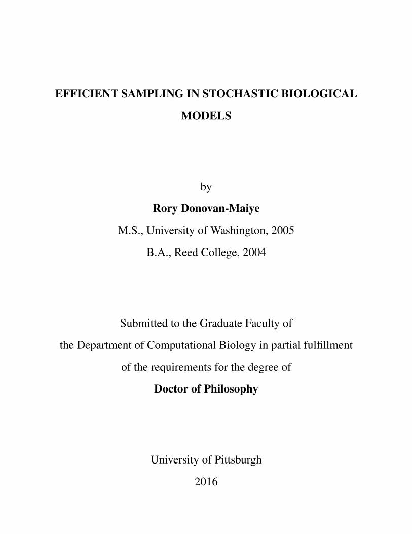
Pairwise discrete Markov random fields are undirected graphs whose nodes can take on a discrete

number of states, and which interact with each other in a pairwise fashion via potential functions

on the edges in the graph. In the context of peptides and proteins, a Markov random field can be

constructed by mapping each residue in the structure to be a node in the graph. Each node takes

on a finite set of conformational states, and edges in the graph capture the relevant interactions

between the states each residue can take. An example of such a graph is shown in Fig. 4.

Markov random fields are a subclass of graphical models that are of particular relevance in

structural biology [54, 57]. Since Markov random fields (MRFs) were introduced as a general-

ization of the Ising model [73], perhaps looking at a simple Ising model formulated as a Markov

9

Edge Potential

Node Potential

Node Potential

Figure 4: An example of a graph induced on an atomic model of a peptide. The graph is constructed

from a PDB structure, using a cutoff distance to determine which edges are included. The nodes

and edges are then populated with potential functions, indexing the single (nodes) and pairwise

(edges) preferences for the nodes to be in particular states. Using nodes that have 11 states each,

one example of an edge potential is shown, along with the node potentials for the nodes it connects.

The potentials are dimensionless numbers which depend exponentially on the energy of the system,

while the different orders of magnitude in the node and edge potentials reflect that in this case, the

intra-residue energies of the node potentials are much stronger that the inter-residue interactions of

characterized by the edge potential. While not shown, each edge and node would similarly possess

such potential functions.

10

random field would be a good introduction to how the formalism works.

X1 X2 X3

�12(x1, x2) �23(x2, x3)

�1(x1) �2(x2) �3(x3)

Figure 4: Factor graph representation of a Markov random field for an Ising model with three sites in anexternal magnetic field. Variables are in circles, and factors are black squares.

and the probability of the system to be in a specific state would be the product of all the factors in the graph:

P =1Z

Y

i j

�i j(xi, x j)Y

k

�k(xk) =1Z�12(x1, x2)�23(x2, x3)�1(x1)�2(x2)�3(x3)

where xi 2 {�1, 1} represents a spin of up or down, �i j(xi, x j) = eJxi x j/kT represents the coupling of neigh-

boring spins, and �i(xi) = emxi/kT represents the coupling of individual spins to the external magnetic field.

The normalization constant, or partition function, is a sum over every possible configuration of the system:

Z =X

x

Y

i j

�i j(xi, x j)Y

k

�k(xk) =X

xi2{�1,1}�12(x1, x2)�23(x2, x3)�1(x1)�2(x2)�3(x3)

One of the great utilities of representing of a probability distribution as a graphical model is that it

permits great visual intuition of statistical properties such as covariance and independence. As a reminder,

we usually say that two variable are statistically independent if and only if P(A, B) = P(A)P(B). Inspecting

the above Ising model we see that none of the variables are statistically independent: the �i j terms do not

allow any such factorization. Even though X1 and X3 are not directly coupled, their behavior is correlated

because they are both coupled to X2.

Another advantage of a graphical representation of the distribution is that it allows us to take advantage

of conditional independencies in the distribution. All variables do not co-vary equally – there is something

fundamentally di↵erent about the interaction between X1 and X2, and between X1 and X3. X1 and X3 do not

directly interact; X2 separates them. In fact if we know the value of X2, then the values of X1 and X3 are no

longer correlated, that is, the values of X1 and X3 are conditionally independent. This is a general property

of Markov random fields, that there is a subset of the graph that we can condition on (or “know the value

of”) that would render two nodes that are not directly connected statistically independent, or disconnected.

Additionally, graphical models let us encode the distribution of states of the system more e�ciently.

Naïvely, to tabulate the energetics of the system, we would need a table that is the size of the number of

6

Figure 5: Factor graph representation of a Markov random field for an Ising model with three sites

in an external magnetic field. Variables are in circles, and factors are black squares.

The graph in Fig. 5 consists of two types of nodes: variables, which can take on different

values (circles) and factors, which are functions of the variables (squares). In this type of graph,

variables only connect to factors and vice versa. The factors are functions of any variable that they

are connected to, and the probability of the system to be in a specific state is proportional to the

product of all the factors in the graph:

P =1Z

∏

i j

φi j(xi, x j)∏

k

φk(xk) =1Zφ12(x1, x2)φ23(x2, x3)φ1(x1)φ2(x2)φ3(x3) (1.1)

In an Ising model, where each variable is a spin that can be either “up” or “down”, the values for

all of the variables xi can be either {−1, 1}. The factors tell us how the states of the individual

variables combine to affect the disposition of the system to be in a certain global configuration.

The factors that connect to only one node, φi(xi) = emxi/kT , represents the coupling of individual

spins to the external magnetic field, and are also known as “node potentials”. The factors that

connect two neighboring nodes, φi j(xi, x j) = eJxi x j/kT represents the coupling of neighboring spins,

and are known as “edge potentials”.

The normalization constant, or partition function in equation 1.1 is a sum over every possible

configuration of the system:

Z =∑

x

∏

i j

φi j(xi, x j)∏

k

φk(xk) =∑

xi∈{−1,1}φ12(x1, x2)φ23(x2, x3)φ1(x1)φ2(x2)φ3(x3) (1.2)

11

It is this sum that is often of interest, due to its deep connection to the free energy of the system, but

it is usually extremely difficult to compute. As we will see, belief propagation offers an attractive

approximation to this sum which can be computed efficiently.

In theory, many nodes can be connected to one factor, if we wished to encode a complicated

interaction that displays no underlying structure. In practice, we will allow a factor to connect to

at most two nodes; MRFs following this restriction are known as pairwise Markov random fields.

I will employ pairwise MRFs exclusively in my work.

One of the great utilities of representing a probability distribution as a pairwise Markov ran-

dom field is that it permits a visual intuition of statistical properties such as covariance and inde-

pendence. As a reminder, we usually say that two variables are statistically independent if and

only if P(A, B) = P(A)P(B); that is, the value of A is unaffected by the value of B. Inspecting the

above Ising model we see that none of the variables are statistically independent: the φi j terms do

not allow any such factorization. Even though X1 and X3 are not directly coupled, their behavior is

correlated because they are both coupled to X2.

The graphical representation of the distribution allows us to take advantage of conditional

independencies in the distribution. All variables do not co-vary equally – there is something fun-

damentally different about the interaction between X1 and X2, and between X1 and X3. X1 and X3

do not directly interact; X2 separates them. In fact if we know the value of X2, then the values of

X1 and X3 are no longer correlated, that is, the values of X1 and X3 are independent, conditioned

on the value of X2. This is a general property of Markov random fields, that there is a subset of the

graph that we can condition on (or “know the value of”) that would render two nodes that are not

directly connected statistically independent, or disconnected. In a pairwise MRF, two nodes are

conditionally independent if there is no factor, or edge, connecting them.

Additionally, graphical models let us encode the distribution of states of the system more

efficiently. Naïvely, to tabulate the energetics of the system, we would need a table that is the size

of the number of values a variable can take (say, k), raised to the number of variables (say, N), i.e

kN , which in our example is 23. Instead, given the structure of the graph, with E edges and N nodes,

we can use E tables of size k2 and N tables of size k to store the possible states of the network. In a

small graph such as our three node example, this “efficient encoding” is actually worse, but as the

size of the graph increases, and the number of states a variable can take increases, the efficiency

12

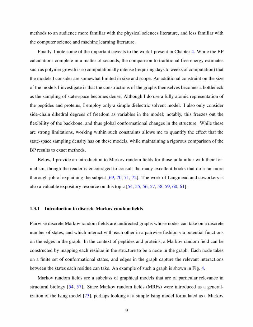
gain scales exponentially. For instance, the gain for an Ising chain of length 10 is about a factor of

10, and for length 100 is a factor of about 1027. The formalism I’ve described for the Ising chain

generalizes straightforwardly to arbitrarily connected graphs where each node in the graph takes

on one of a certain set of discrete values.

values a variable can take, raised to the number of variables (here, 23). Instead, given the structure of the

graph, we can use 2 tables of size 23 and 3 tables of size 2. In such a small graph, this “e�cient encoding”

is actually worse, but as the size of the graph increases, and the number of states a variable takes increases,

the e�ciency gain scales exponentially. For instance, the gain for an Ising chain of length 10 is about a

factor of 10, and for length 100 is a factor of about 1026. The formalism I’ve described for the Ising chain

generalizes straightforwardly to arbitrarily connected graphs where each node in the graph takes on one of

a certain set of discrete values.

X1 X2 X3

X4X5X6

X7 X8

(a)

X1

X2

X3

X4 X5

X6

X7

X8

X9

(b)

Figure 5: More complicated graphs for pairwise Markov random fields. (a) Ising chain Markov randomfield with N sites. Variables are in circles, with node potentials implied. Edge-potential factors are implied

to be along the edges that are present. (b) Arbitrarily connected Markov random field. Variables are incircles, with node potentials implied. Edge-potential factors are implied to be along the edges that are

present.

However, using discrete states isn’t always the most natural way to encode the values a variable can

take. For instance, many random variables are distributed normally, and characterizing those variables by

arbitrarily discretizing the distributions is not ideal, since discretization will introduce errors, and also since

the computational cost of the calculation scales with the number of states a variable can take. Rather, a

di↵erent, but very similar class of graphical models have been developed for variables that are each drawn

from a Gaussian distribution, which will be discussed in Section III B.

The most computationally taxing aspect of using graphical models is computing the normalization con-

stant, or partition function Z. In fact, since the computational e↵ort scales exponentially in the number

of variables and the number of states, for any but a small class of simple graphs, an exact calculation is

computationally intractable. However, approximation schemes exist that run in reasonable times and often

yield results that are quite close the the exact computation [55]. Moreover, di↵erent approximation schemes

can be used, some that provably overestimate the exact value of the partition function [56, 57], and some

that provably underestimate it [58–60]; combined, they provide bounds on an approximation error (new

7

(a)

values a variable can take, raised to the number of variables (here, 23). Instead, given the structure of the

graph, we can use 2 tables of size 23 and 3 tables of size 2. In such a small graph, this “e�cient encoding”

is actually worse, but as the size of the graph increases, and the number of states a variable takes increases,

the e�ciency gain scales exponentially. For instance, the gain for an Ising chain of length 10 is about a

factor of 10, and for length 100 is a factor of about 1026. The formalism I’ve described for the Ising chain

generalizes straightforwardly to arbitrarily connected graphs where each node in the graph takes on one of

a certain set of discrete values.

X1 X2 X3

X4X5X6

X7 X8

(a)

X1

X2

X3

X4 X5

X6

X7

X8

X9

(b)

Figure 5: More complicated graphs for pairwise Markov random fields. (a) Ising chain Markov randomfield with N sites. Variables are in circles, with node potentials implied. Edge-potential factors are implied

to be along the edges that are present. (b) Arbitrarily connected Markov random field. Variables are incircles, with node potentials implied. Edge-potential factors are implied to be along the edges that are

present.

However, using discrete states isn’t always the most natural way to encode the values a variable can

take. For instance, many random variables are distributed normally, and characterizing those variables by

arbitrarily discretizing the distributions is not ideal, since discretization will introduce errors, and also since

the computational cost of the calculation scales with the number of states a variable can take. Rather, a

di↵erent, but very similar class of graphical models have been developed for variables that are each drawn

from a Gaussian distribution, which will be discussed in Section III B.

The most computationally taxing aspect of using graphical models is computing the normalization con-

stant, or partition function Z. In fact, since the computational e↵ort scales exponentially in the number

of variables and the number of states, for any but a small class of simple graphs, an exact calculation is

computationally intractable. However, approximation schemes exist that run in reasonable times and often

yield results that are quite close the the exact computation [55]. Moreover, di↵erent approximation schemes

can be used, some that provably overestimate the exact value of the partition function [56, 57], and some

that provably underestimate it [58–60]; combined, they provide bounds on an approximation error (new

7

(b)

Figure 6: More complicated graphs for pairwise Markov random fields. (a) Ising chain Markov

random field with N sites. Variables are in circles, with node potentials implied. Edge-potential

factors are implied to be along the edges that are present. (b) Arbitrarily connected Markov random

field. Variables are in circles, with node potentials implied. Edge-potential factors are implied to

exist along the edges that are present.

One of the most computationally taxing aspects of using graphical models is computing the

normalization constant, or partition function Z, in equation 1.2. For example, in an Ising model

with 100 nodes, a naïve computation of the partition function entails a sum over 2100 terms. Due

to this exponential scaling, for any but a small class of simple graphs an exact calculation is com-

putationally intractable. However, approximation schemes exist that run in reasonable times and

often yield results that are quite close to the exact computation.

In particular, an approximation known as loopy belief propagation can quickly produce ap-

proximations to the partition function that are startlingly good [64, 74]. As discussed above, for

arbitrary MRFs, loopy belief propagation is not guaranteed to converge to an answer, and even if

it does, that answer is not guaranteed to be within a given tolerance of the exact result.

13

2.0 WEIGHTED ENSEMBLE IN NON-SPATIAL SYSTEMS

2.1 INTRODUCTION

As discussed in Chapter 1, there is significant interest in accelerating the sampling of stochastic

systems biology models. There are many approaches to this challenging problem, ranging from

methods that accelerate the dynamics themselves using approximations [22, 23, 24, 25, 26, 27,

28, 29], to importance sampling methods [30, 31, 32, 33, 34], to forward flux-based methods and

umbrella sampling methods[21, 35, 36, 37, 75, 76, 39, 38].

The approach we take here, of weighted ensemble sampling, originally found application in

the field of structural biology simulation [44, 45, 46, 47, 48, 49, 50, 51], and is most similar in

spirit to the forward flux forward flux sampling [37] and non-equilibrium umbrella sampling [39]

methods, though many related approaches exist [40, 41, 42, 43].

The weighted ensemble approach distinguishes itself in its combination of relative simplicity

and potential flexibility in sampling rare events. Here we apply it to study rare events in model sys-

tems of stochastic kinetic chemical reactions. These models range in complexity from one species

and two reactions, to 354 species and 3680 reactions. For the systems studied, WE proves many

orders of magnitude faster than SSA simulation alone, offers linear parallel scaling, returns full

distributions of desired species at arbitrary times, and can yield mean first passage times (MFPTs)

via the setup of a feedback steady-state.

14

2.2 METHODOLOGY

The methods employed are described immediately below, while the models are specified in Sec.

2.3.

2.2.1 Stochastic Chemical Kinetics & BioNetGen

Stochastic chemical kinetics occupies a middle-ground in the realm of chemical simulation, be-

tween very explicit, and costly, molecular dynamics (MD) simulations and the deterministic for-

malism of reaction rate equations (RRE). Stochastic chemical kinetics attempts to account for the

randomness inherent in chemical reactions, without trying to explicitly model the spatial structure

of the reacting species. It is many orders of magnitude faster than MD simulations, but much

slower than the RRE approach. It is an ideal method to use for modeling the effects of low con-

centrations (or copy numbers) of chemical reactants, while ignoring the effects of specific spatial

distribution.

Stochastic chemical kinetics models can be solved exactly for sufficiently simple systems using

the Chemical Master Equation (CME), and approximately (for all systems) using Gillespie’s direct

stochastic simulation algorithm (SSA) [19, 20, 16]. The SSA samples the CME exact solution

by modeling stochastic chemical kinetics in a straightforward manner, and yields trajectories of

species concentrations that converge to the RRE method in the limit of large amounts of reactants.

In brief, the SSA iteratively and stochastically determines which reaction fires at what time by

sampling from the exponential distribution of waiting times between reactions. For a detailed

explanation of the SSA, see [16].

We employ the rule-based modeling and simulation package BioNetGen [53] to simulate both

our toy and complex models. Rule-based modeling languages allow the specification of biochem-

ical networks based on molecular interactions. Rules that describe those interactions can be used

to generate a reaction network that can be simulated either as RREs or using the SSA, or the rules

can be used directly to drive stochastic chemical kinetics simulations. BioNetGen has been applied

to a variety of systems, such as the aggregation of membrane proteins by cytosolic cross-linkers

in the LAT-Grb2-SOS1 system [77], the single-cell quantification of IL-2 response by effector and

15

regulatory T cells [78], the analysis and verification of the HMGB1 signaling pathway [79], the

role of scaffold number in yeast signaling systems [80], and the analysis of the roles of Lyn and Fyn

in early events in B cell antigen receptor signaling [81]. We employ BioNetGen’s implementation

of the direct SSA to propagate the dynamics in our systems.

2.2.2 Weighted Ensemble (WE)

WE is a general-purpose protocol used in molecular dynamics simulations [45, 46, 47, 49, 50, 51]

that we adapt here to the efficient sampling of dynamics generated by chemical kinetic models.

In brief, WE employs a strategy of “statistical natural selection” using quasi-independent parallel

simulations which are coupled by the intermittent exchange of information. The intermittency

leads directly to linear parallel scaling. Importantly, the simulations are coupled via configuration

space (essentially the “phase space” of the system in physics language or the “state-space” in cell

and population modeling). This type of coupling permits both efficiency and a large degree of scale

independence. The efficiency results from distributing trajectories to typically under-sampled parts

of the space, while scale independence is afforded because every type of system has a configuration

or state-space.

WE’s strategy of statistical natural selection or statistical ratcheting is schematized in Fig. 1. A

detailed heuristic description of the algorithm is provided in Chapter 1, while pseudocode is listed

below. It is worth emphasizing that the iterative resampling upon which the algorithm is based is

statistically exact, guaranteeing an unbiased estimate of the probability distributions for a broad

class of stochastic processes [46].

The weighted ensemble algorithm can be outlined fairly concisely. Let Mtarg be the target

number of segments in each bin, Nbins the number of bins, whose geometry are defined by the grid

Ggrid, τ the time-step of an iteration of WE, and Niters the total number of iterations of WE. The

WE procedure also requires an initial state of the system, x0, which in our case is a list of the

concentrations of all the chemical species in the system.

procedure WE(Niters, τ,Ggrid,Mtarg, x0)

for i = 1 . . .Niters do

for each populated bin in Ggrid do

16

propagate dynamics for all trajectories

update bin populations

for each bin in Ggrid do

if bin population = 0 or Mtarg then

do nothing

else if bin population < Mtarg then

replicate trajectories until bin pop. = Mtarg

maintain sum of weights in each bin

else if bin population > Mtarg then

merge trajectories until bin pop. = Mtarg

maintain sum of weights in each bin

save coordinates and weights of each trajectory

return trajectory coordinates & weights for each iter.

The replicating and merging of trajectories in the above algorithm are done randomly, according

to the weight of each trajectory segment in a given bin, which has been shown not to bias the

dynamics of the ensemble [44, 47].

Setting up a WE simulation requires selection of state-space binning, trajectory multiplicity,

and timing parameters. In our simulations, we chose to divide the state-space of an N-dimensional

system into one- or two-dimensional regular grids of non-overlapping bins. It is possible to use

non-Cartesian bins, and to adaptively change the bins during simulation [46, 49], but for simplicity

we did not pursue any such optimization. Specific parameter choices for each model are given in

Sec. 2.3.

When WE is used to manage an ensemble of trajectories, there are two time-scales of im-

mediate concern: the period at which trajectory coordinates are saved, and the period τ at which

ensemble operations are performed. These two time-scales can be different, but for simplicity we

set them to be the same, and select τ such that it is greater than the inverse of the average event

firing rate for the SSA. When we refer to the time-step, or iteration of a process, we are referring

to the τ of Fig. 1.

WE can be employed in a variety of modes to address different questions. Originally developed

17

to monitor the time evolution of arbitrary initial probability distributions [44], i.e. non-stationary

non-equilibrium systems, WE was generalized to efficiently simulate both equilibrium and non-

equilibrium steady-states [47]. In steady-state mode, mean first passage times (MFPTs) can be es-

timated rapidly based on simulations much shorter than the MFPT using a simple rigorous relation

between the flux and MFPT [47]. Steady-states can be attained rapidly, avoiding long relaxation

times, by using the inter-bin rates computed during a simulation to estimate bin probabilities ap-

propriate to the desired steady-state; trajectories are then reweighted to conform to the steady-state

bin probabilities [47]. Both of these methods are described in more detail below.

2.2.2.1 Basic WE: Probability Distribution Evolving in Time Perhaps the simplest use of

a weighted ensemble of trajectories is to better sample rare states as a system evolves in time,

specifically the states corresponding to extreme values of the binning coordinate. The SSA itself

samples the exact distribution, but its sampling is concentrated about the mode(s) of the distri-

bution. The SSA naturally – and correctly – samples rare states infrequently. By using WE to

split up the state-space, however, one can resample the distribution at every time step τ, selecting

those trajectories that advance along a progress coordinate for more detailed study, but doing so

without applying any forces or biasing the trajectories or the distribution. Essentially, WE appro-

priates much of the effort that brute-force SSA devotes to sampling the central component of the

distribution, repurposing it to obtain better estimates of the tails.

This basic use of WE requires none of the “tricks” we apply in later sections, such as using

reweighting techniques to accelerate obtaining a steady-state. We apply basic WE to some of our

systems – particularly, but not exclusively, to those that are not bistable.

2.2.2.2 Steady-State The mean first passage time (MFPT) from state A to state B is a key

observable. It is equal to the inverse of the flux (of probability density) from state A to state B in

steady-state [82],

MFPTA→B =1

Fluxss(A→ B). (2.1)

This relation provides the weighted ensemble approach the ability to calculate MFPTs in a straight-

forward manner. During a WE run, when any trajectories (and their associated weights) reach a

designated target area of state-space (or “state B”), they are removed and placed back in the initial

18

state (“state A”). Eventually, such a process will result in a steady-state flow of probability from

state A to state B that does not change in time (other than with stochastic noise).

Reweighting. The waiting time to obtain a steady-state constrains the efficiency of obtaining

a MFPT by measuring fluxes via equation 2.1. This waiting time can vary from the relatively

short time scale of intra-state equilibration for simple systems, to much longer time-scales, on the

order of the MFPT itself for more complicated systems. To reduce this waiting time, we use the

steady-state reweighting procedure of Bhatt et al. [47]. This method measures the fluxes between

bins to obtain a rate-matrix for transitions between bins, and uses a Markov formulation to infer a

steady-state distribution from the (noisy) data available.

For instance, let {wi} be the set of bin weights (i.e the sum of the weights of the trajectories

in each bin), and let {wssi } be the set of steady-state values of the bin weights. If fi j is the flux of

weight into bin i from bin j, then in steady-state, since the flux out of a bin is equal to the flux into

it,

dwssi

dt=

∑

j

(f ssi j − f ss

ji

)=

∑

j

(ki jwss

j − k jiwssi

)= 0 . (2.2)

Since the flux of weight into bin i from bin j is the product of a (constant) rate and the (current)

weight in a bin, i.e. fi j = ki j w j (true for both steady state and not), we can use Eq. 2.2 to find the

inter-bin rates. By measuring the inter-bin fluxes and the bin weights, we can approximately infer

the transition rates, and then find a set of weights that satisfy Eq. 2.2. Once the set of bin weights

is found, the weights of the individual trajectories in the bins are rescaled commensurately. This

reweighting process should not be confused with a resampling process (such as basic WE splitting

and merging) which does not change the distribution.

The steady-state distribution of weights thus inferred is not necessarily the true steady-state of

the system, but tends to be closer to it than the distribution was prior to reweighting, and an iterative

application of this procedure can converge to the true distribution fairly rapidly. In practice it has

been shown to accelerate the system’s evolution to a true steady-state by orders of magnitude in

some cases [47].

19

2.2.3 Estimation of Computational Efficiency

Since it is important to assess new approaches quantitatively, we compare the speedup in comput-

ing time from weighted ensemble to a brute-force simulation, (i.e. SSA). For a given observable

(e.g., the fraction of probability in a specified tail of the distribution) and a desired precision, we

estimate the efficiency using the ratio:

E Bdynamics time in brute-force SSA

dynamics time in WE-SSA(2.3)

Since both WE and brute-force use the same dynamics engine/software, we can estimate the

speedup of WE over brute-force by just keeping track of how much total “dynamics time” was

simulated in each. We employ this measure when estimating the advantage of using WE to inves-

tigate the tails of probability distributions, as well as for finding MFPTs in bistable systems.

Another measure of efficiency we employ for MFPT estimation gauges how fast WE attains a

result that is within 50% of the true result (determined from exact or extensive brute-force calcu-

lation):

E50% Bdynamics time in brute-force SSA to get ± 50% exact

dynamics time in WE-SSA to get ± 50% exact. (2.4)

This is an assessment of how well WE can extract rough estimates of long time-scale behavior

from simulations that are much shorter than those timescales.

Brute-force SSA simulations can be run for long times without seeing a transition from one

macro-state to another. To take account of the brute-force simulations where no transitions oc-

curred we use a maximum likelihood estimator for the transition time, based on an exponential

distribution of waiting times [83], which is a valid approximation for the one-dimensional and

two-state systems studied below:

µMLE =

(1 − n

N

)T +

1n

n∑

i=1

ti

σµ =µMLE√

n

(2.5)

where T is the length of the brute-force simulations, N is the number of these simulations per-

formed, n is the number of these simulations in which a transition from one state to another is

observed, and ti are the times at which the transition is observed.

20

2.2.4 Limitations of Our Implementation

We used two different implementations of the weighted ensemble framework: WESTPA, written in

Python, is the most feature-rich and stable [51], which will be available at http://chong.chem.

pitt.edu/WESTPA. Another, written by Bin Zhang [45] and modified by us, is written in C, and

is faster though less robust, and is available at http://donovanr.github.com/WE_git_code.

Weighted ensemble (WE), as a scripting-level approach, inherently adds some unavoidable

overhead to the runtime of the dynamics. This overhead, in theory, is quite minimal: stopping,

starting, merging, and splitting trajectories are not computationally costly operations. A key issue

in practical implementations, though, is how long the algorithm actually takes to run, i.e the wall-

clock running-time for dynamics (here, the SSA).

In practice, overhead can be significant for very simple systems, for the sole reason that reading

and writing to disk takes so much time compared to how long it takes to run the dynamics of small

models. In our implementation, data is passed from the dynamics engine to WE by reading and

writing files to disk. This handicap is an artifact of our interface, which could, with minimal work,

be modified to something more efficient. As a proof-of-principle, the version of WE written in C

was modified, for the Schlögl reactions and the futile cycle, to contain hard-coded versions of the

Gillespie direct algorithm for those systems, so as to obviate the I/O between WE and BNG. With

these modifications, it was difficult to ascertain any significant overhead costs at all, and our runs

completed in a matter of seconds. We also note that as model complexity increases and more time

is devoted to dynamics, the overhead problem becomes negligible. Practical applications of WE

will, by nature, target models where dynamics are expensive, rather than toy models, where they

are cheap.

2.3 MODELS & RESULTS

We study four different models, ranging in complexity from two chemical reactions governing one

chemical species, to 3680 reactions governing 354 species. The models we employ are coupled

stochastic chemical reactions, which we implement and simulate in BioNetGen using the SSA [19,

21

20, 16]. As depicted in Fig. 1, these simulations are, in turn, managed by a weighted ensemble

procedure.

2.3.1 Enzymatic Futile Cycle

2.3.1.1 Model The enzymatic futile cycle is a simple and robust model that can, in certain

parameter regimes, exhibit qualitatively different behavior due to stochastic noise [84, 85]. This

signaling motif can be seen in biological systems including GTPase cycles, MAPK cascades, and

glucose mobilization [84, 86, 87].

The enzymatic futile cycle studied here is modeled by:

E1 + S 1

k f−⇀↽−k f

B1ks−→ E1 + S 2

E2 + S 2

k f−⇀↽−k f

B2ks−→ E2 + S 1

(2.6)

where k f = 1.0 and ks = 0.1. Here S 1 can bind to its enzyme E1, and in the bound form, B1, (i.e.

B1 = E1 · S 1), it can be converted to S 2, and then dissociate (and similarly for S 2 −→ S 1). The total

amount of substrate, S 1 + S 2, is conserved, as are the amounts of the different enzymes E1 and E2,

of which is supplied only one of each kind, thus (S 1 + B1) + (S 2 + B2) = 100. Following Kuwahara

and Mura [30], in the specific system we look at, we set S 1 + S 2 = 100 and E1 + B1 = E2 + B2 = 1.

Thus constrained, the above system of reactions can be solved by an approximately 400-state

chemical master equation (CME), to obtain an exact probability density for all times when initial-

ized from an arbitrary starting point. We start the system at S 1 = S 2 = 50 and E1 = E2 = 1, and

are interested in the probability distribution of S 1 after 100 seconds, that is, P(S 1 = x, t = 100).

2.3.1.2 WE Parameters The WE data was generated using 101 bins of unit width on the co-

ordinate S 1. We employed 100 trajectory segments per bin that were run for 100 iterations of a

τ = 1 s time-step, with no reweighting events. The brute-force data is from 10,200 100-second

runs, which is an equivalent amount of dynamics to compute as the single WE run, if all the bins

were full all the time. However, since the bins take some time to fill up, the WE run employed only

840,000 one-second segments, which makes the comparison to brute-force SSA more than fair.

22

2.3.1.3 Results Fig. 7 shows that the brute-force SSA is unable to sample values of S 1 much

outside the range 30 < S 1 < 70, whereas the WE method is able to accurately sample the entire

distribution. Waiting for the brute-force approach to sample the tails would take ∼ 1/P(tail) ∼1/10−23 ∼ 1023 brute-force runs. With a conservative estimate of ∼104 runs per second, it would

take ∼1019 seconds, or many times the age of the universe, for brute-force SSA to sample the tails

at all. WE takes 2–3 seconds to sample them (note the comparison to exact distribution provided

by the CME), for an approximate efficiency increase E ∼ 1018.

For the sake of clarity, error-bars were omitted from Fig. 7. Over most of the data range, the

error is too small to see on the plot. In the tails (of both SSA and WE-SSA) the error is not com-

putable from a single run, since there are plot points comprised of only a single trajectory. The

error in the estimate of the distribution can be inferred visually from the data’s departure from the

CME exact solution. For SSA, however, generating uncertainties far all values is essentially impos-

sible. When computing quantitative observables reported below, we employ multiple independent

runs to procure standard errors in our estimate.

From the distribution, we are able to read off useful statistics. For instance, in the spirit of

Kuwahara and Mura [30], and Petzold and Gillespie et al. [31], one might desire to know the

probability of the futile cycle to have a value of S 1 > 90 at ∆t = 100, which we will denote

as p>90. Since WE gives an accurate estimate of P(x, t) on an arbitrarily precise spatio-temporal

grid, all that is required to find p>90 is to sum up the area under the state of interest: we find

p>90 = 2.47 × 10−18 ± 3.4 × 10−19 at one standard error, as computed from ten replicates of the

single WE run plotted in Fig. 7. The CME gives an exact value of 2.72×10−18. Following Gillespie

et al. in [31], the approximate number of normal SSA runs needed to estimate this observable with

comparable error is nSSAp>90

= p>90/(σp>90)2 = 2.72 × 10−18/(3.4 × 10−19)2 = 2.4 × 1019 SSA runs.

Using ten replicate runs, WE is able to sample it using a total of 8,317,000 trajectory segments,

which is computationally equivalent to 83,170 brute-force trajectories, resulting in an increase in

sampling efficiency by a factor of E ∼ 2.4×1019/83, 170 ∼ 3×1014 for this observable at this level

of accuracy.

Since WE gives the full distribution, from the same data we can also find other rare event

statistics. For example, we might also wish to compute the probability that S 1 ≤ 25 at ∆t = 100,

which we will call p≤25. From the same data described in the preceding paragraph, we can find

23

ÈÈÈÈÈÈÈÈÈÈÈÈÈÈÈÈÈÈÈÈÈÈÈÈÈÈÈÈÈÈÈÈÈÈÈÈÈÈÈÈÈÈÈÈÈÈÈÈÈÈÈÈÈÈÈÈÈÈÈÈÈÈÈÈÈÈÈÈÈÈÈÈÈÈÈÈÈÈÈÈÈ

ÈÈÈÈÈÈÈÈÈÈÈÈÈÈÈÈÈÈÈ

µ µµµµµµµµµµµµµ

µµµµµµµµµµµµµµµµµµµµ µ

CME

È WE-SSA

µ SSA

0 20 40 60 80 10010-26

10-21

10-16

10-11

10-6

0.1

Population of S1 at t = 100 secs.

Probability

Figure 7: The probability distribution of S 1 in the Enzymatic Futile Cycle System, after t = 100

seconds, when initialized from a delta function at S 1 = 50, E1 = E2 = 1 at t = 0. The exact

solution, procured via the chemical master equation (CME), is compared to data obtained using

the SSA in a weighted ensemble run (WE-SSA), and to ordinary SSA, when each are given equal

computation time. WE data is from a single run. Error bars are not plotted; for a discussion of

uncertainties, see Sec. 2.3.1.3. The noise in the tail of the SSA points and gap in coverage is

indicative of the high variance of SSA for rare events.

24

p≤25 = 1.35×10−7±1.5×10−8 at one standard error. The CME gives an exact value of 1.26×10−7.

Again, estimating the number of SSA runs necessary to determine the same observable with similar

accuracy as in [31], we find nSSAp≤25

= p≤25/(σp≤25)2 = 1.26 × 10−7/(1.5 × 10−8)2 = 6.0 × 108 SSA

runs. Our weighted ensemble calculation used the computational equivalent of 83,170 brute-force

trajectories, resulting in an increase in sampling efficiency by a factor of E ∼ 6.0 × 108/83, 170 ∼7 × 103 for this observable at this level of accuracy.

Kuwahara and Mura [30], and Petzold and Gillespie et al. [31] define a quantity closely related

to those computed above: the probability of a system to pass from one state to another in a certain

time: P(xi → x f |∆t) [30, 31, 32, 33, 34]. This is subtly different than just measuring areas under

a distribution, since a trajectory is terminated, and removed from the ensemble, if it successfully

reaches the target. To make a direct comparison to this statistic, we implemented in WE an absorb-

ing boundary condition at the target state S 1 = 25. Using ten WE runs, we find that the probability

of reaching the S 1 = 25 within 100 seconds, which we call pabs(25), is 1.61 × 10−7 ± 1.93 × 10−8

at one standard error. The CME with an absorbing boundary condition at S 1 = 25 gives an exact

value of 1.738 × 10−7. As above, we estimate the number of brute-force SSA runs needed to attain

a comparable estimate as nSSApabs(25)

= pabs(25)/(σpabs(25))2 = 1.738 × 10−7/(1.93 × 10−8)2 = 4.66 × 108

SSA runs. In total, the ten WE runs used 6,342,600 trajectory segments, which is computa-

tionally equivalent to 63,426 brute-force trajectories. This yields an increase in efficiency of

E ∼ 4.66 × 108/63, 426 ∼ 7 × 103 for this observable at this level of accuracy.

For the above statistic, Gillespie et al. report an efficiency gain of 7.76 × 105 over brute-force

SSA[31]. Direct comparisons of efficiency gain between wSSA and WE are difficult, even when

focussing on the same observable in the same system. Many factors contribute to this, notably that

WE is not optimized in a target-specific manner, as wSSA historically has been. Further, in its

simplest form, WE yields a full space/time distribution of trajectories, from which it is possible to

calculate rare event statistics for arbitrary states, which need not be specified in advance.

2.3.2 Schlögl Reactions

2.3.2.1 Model The Schlögl reactions are a classic toy-model for benchmarking stochastic sim-

ulations of bistable systems [88, 89, 90]. They are two coupled reactions with one dynamic species,

25

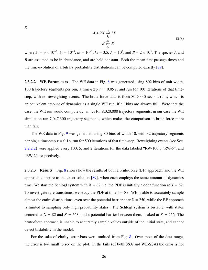
X:A + 2X

k1−⇀↽−k2

3X

Bk3−⇀↽−k4

X(2.7)

where k1 = 3 × 10−7, k2 = 10−4, k3 = 10−3, k4 = 3.5, A = 105, and B = 2 × 105. The species A and

B are assumed to be in abundance, and are held constant. Both the mean first passage times and

the time-evolution of arbitrary probability distributions can be computed exactly [89].

2.3.2.2 WE Parameters The WE data in Fig. 8 was generated using 802 bins of unit width,

100 trajectory segments per bin, a time-step τ = 0.05 s, and run for 100 iterations of that time-

step, with no reweighting events. The brute-force data is from 80,200 5-second runs, which is

an equivalent amount of dynamics as a single WE run, if all bins are always full. Were that the

case, the WE run would compute dynamics for 8,020,000 trajectory segments; in our case the WE

simulation ran 7,047,300 trajectory segments, which makes the comparison to brute-force more

than fair.

The WE data in Fig. 9 was generated using 80 bins of width 10, with 32 trajectory segments

per bin, a time-step τ = 0.1 s, run for 500 iterations of that time-step. Reweighting events (see Sec.

2.2.2.2) were applied every 100, 5, and 2 iterations for the data labeled “RW-100”, “RW-5”, and

“RW-2”, respectively.

2.3.2.3 Results Fig. 8 shows how the results of both a brute-force (BF) approach, and the WE

approach compare to the exact solution [89], when each employs the same amount of dynamics

time. We start the Schlögl system with X = 82, i.e. the PDF is initially a delta function at X = 82.

To investigate rare transitions, we study the PDF at time t = 5 s. WE is able to accurately sample

almost the entire distributions, even over the potential barrier near X = 250, while the BF approach

is limited to sampling only high probability states. The Schlögl system is bistable, with states

centered at X = 82 and X = 563, and a potential barrier between them, peaked at X = 256. The

brute-force approach is unable to accurately sample values outside of the initial state, and cannot

detect bistability in the model.

For the sake of clarity, error-bars were omitted from Fig. 8. Over most of the data range,

the error is too small to see on the plot. In the tails (of both SSA and WE-SSA) the error is not

26

computable from a single run, since there are plot points comprised of only a single trajectory.

Multiple runs are consistent with the data shown. The error in the estimate of the distribution can

be inferred visually from the data’s departure from the CME exact solution. When computing

quantitative observables below, we employ multiple independent runs to procure standard errors in

our estimate.

WE yields the full, unbiased probability distribution, but we again examine an observable in

the spirit of that investigated by Petzold, Gillespie, and coworkers[30, 31, 32, 33, 34], i.e. the

probability that the progress coordinate is beyond a certain threshold at a specified time, which is

a simple summation of the distribution over the state of interest. From ten replicates of the Schlögl

run plotted in Fig. 8, the probability that X ≥ 700 at t = 5 seconds, i.e. P(X ≥ 700, t = 5 s),

which we call p≥700, is 1.143 × 10−9 ± 4.7 × 10−11 at one standard error. The CME exact

value is 1.148 × 10−9. Following [31], we can estimate the number of brute-force SSA runs that

would be needed to find p≥700 at a similar level of accuracy as nSSAp≥700

= p≥700/(σp≥700)2 = 1.148 ×

10−9/(4.7 × 10−11)2 = 5.3 × 1011 SSA runs. We can then estimate an improvement in efficiency of

using WE over brute-force of E ∼ 5.3× 1011/802, 000 ∼ 7× 105 for this observable at this level of

accuracy.

We also estimate the mean first passage time (MFPT) of the Schlögl system, which can be

computed exactly [89]. Weighted ensemble can estimate the MFPT using Eq. 2.1 when the system

is put into a steady-state. For the run that was reweighted every 100 iterations, Fig. 9 shows the

WE estimates of the flux from the initial state (X = 82) to the final state (X ≥ 563) converge to the

exact value in about 100 iterations of weighted ensemble splittings and mergings, which is when

the system relaxes from its delta-function initialization to a steady-state. The attainment of steady-

state is accelerated by more frequent reweighting (see Sec. 2.2.2.2 on reweighting), as is shown in

Fig. 9 in the runs that are reweighted every 2 and 5 iterations. These more frequently reweighted

runs yield fluxes close to the exact value within about 30 iterations.

To quantify WE’s improvement over brute-force in the estimate of the MFPT, we use the mea-

sure E50% defined in Sec. 2.2.3. A brute-force estimate of the MFPT would require, optimistically,

computing an amount of dynamics on the order of the MFPT itself (approximately 5 × 104 sec-

onds). Since transitions in this system follow an exponential distribution, the standard deviation

of the first passage times is equal to the mean of them. WE’s estimate of the MFPT is within 50%

27

ÈÈÈÈÈ

ÈÈ

È

ÈÈÈ

ÈÈÈÈÈÈÈÈÈÈÈÈÈÈÈÈÈÈÈÈÈÈÈÈÈÈÈÈÈÈÈÈÈÈÈÈÈÈÈÈÈÈÈÈÈÈÈÈÈÈÈÈÈÈÈÈÈÈÈÈÈÈÈÈÈÈÈÈÈÈÈÈÈÈÈÈÈÈÈÈÈÈÈÈÈÈÈÈÈÈÈÈÈÈÈÈÈÈÈÈÈÈÈÈÈÈÈÈÈÈÈÈÈÈÈÈÈÈÈÈÈÈÈÈÈÈÈÈÈÈÈÈÈÈÈÈÈÈÈÈÈÈÈÈÈÈÈÈÈÈÈÈÈÈÈÈÈÈÈÈÈÈÈÈÈÈÈÈÈÈÈÈÈÈÈÈÈÈÈÈÈÈÈÈÈÈÈÈÈÈÈÈÈÈÈÈÈÈÈÈÈÈÈÈÈÈÈÈÈÈÈÈÈÈÈÈÈÈÈÈÈÈÈÈÈÈÈÈÈÈÈÈÈÈÈÈÈÈÈÈÈÈÈÈÈÈÈÈÈÈÈÈÈÈÈÈÈÈÈÈÈÈÈÈÈÈÈÈÈÈÈÈÈÈÈÈÈÈÈÈÈÈÈÈÈÈÈÈÈÈÈÈÈÈÈÈÈÈÈÈÈÈÈÈÈÈÈÈÈÈÈÈÈÈÈÈÈÈÈÈÈÈÈÈÈÈÈÈÈÈÈÈÈÈÈÈÈÈÈÈÈÈÈÈÈÈÈÈÈÈÈÈÈÈÈÈÈÈÈÈÈÈÈÈÈÈÈÈÈÈÈÈÈÈÈÈÈÈÈÈÈÈÈÈÈÈÈÈÈÈÈÈÈÈÈÈÈÈÈÈÈÈÈÈÈÈÈÈÈÈÈÈÈÈÈÈÈÈÈÈÈÈÈÈÈÈÈÈÈÈÈÈÈÈÈÈÈÈÈÈÈÈÈÈÈÈÈÈÈÈÈÈÈÈÈÈÈÈÈÈÈÈÈÈÈÈÈÈÈÈÈÈÈÈÈÈÈÈÈÈÈÈÈÈÈÈÈÈÈÈÈÈÈÈÈÈÈÈÈÈÈÈÈÈÈÈÈÈÈÈÈÈÈÈÈÈÈÈÈÈÈÈÈÈÈÈÈÈÈÈÈÈÈÈÈÈÈÈÈÈÈÈÈÈÈÈÈÈÈÈÈÈÈÈÈÈÈÈÈÈÈÈÈÈÈÈÈÈÈÈÈÈÈÈÈÈÈÈÈÈÈÈÈÈÈÈÈÈÈÈÈÈÈÈÈÈÈÈÈÈÈÈÈÈÈÈÈÈÈÈÈÈÈÈÈÈÈÈÈÈÈÈÈÈÈÈÈÈÈÈÈÈÈÈÈÈÈÈÈÈÈÈÈÈÈÈÈÈÈÈÈÈÈÈÈÈÈÈÈÈÈÈÈÈÈÈÈÈÈÈÈÈÈÈÈÈÈÈÈÈÈÈÈÈÈÈÈÈÈÈÈÈÈÈÈÈÈÈ

ÈÈÈÈÈÈÈÈÈÈÈ

ÈÈÈÈÈÈÈÈÈÈÈÈÈÈÈÈÈÈÈÈÈÈÈÈÈÈÈÈÈÈÈÈÈÈ

ÈÈÈÈÈÈ

ÈÈÈÈÈ

È

È

ÈÈÈÈ

È

ÈÈ

ÈÈÈ

ÈÈÈÈÈÈÈÈ

È

È

È

ÈÈ

µµµµµµµµµµµµµµµµµµµµµµµµµµµµµµµµµµµµµµµµµµµµµµµµµµµµµµµµµµµµµµµµµµµµµµµµµµµµµµµµµµµµµµµµµµµµµµµµµµµµµµµµµµµµµµµµµµµµ

µµµµµµµµµµµµµµµµµµµµµµµµµµµµµµµ µ

CME

È WE-SSA

µ SSA

0 200 400 600 80010-18

10-15

10-12

10-9

10-6

0.001

1

Population of X at t = 5 secs.

Probability

Figure 8: The probability distribution of X in the Schlögl system, at t = 5 seconds, when initialized

from a delta function at X = 82. The exact solution from the chemical master equation is compared

to data obtained using the SSA in a weighted ensemble run (WE-SSA), and to ordinary SSA. WE

data is from a single run. For a discussion of uncertainties, see Sec. 2.3.2.3. The noise in the tail

of the SSA points and gap in coverage is indicative of the high variance of SSA for rare events.

28

of the exact value after about 30 iterations of WE simulation, at which point about 1100 trajectory

segments have been propagated, which is equivalent to propagating about 110 seconds of brute-

force dynamics. Thus we find E50% ∼ 5 × 104/110 ≈ 500. As can be seen in Fig. 9, this value

is about a 3–5 fold increase over the WE results when reweighting very infrequently (every 100

iterations).

WE-SSA, RW-100

WE-SSA, RW-5

WE-SSA, RW-2

Exact

0 100 200 300 400 50010-12

10-10

10-8

10-6

10-4

0.01

1

Iteration

Flux

Figure 9: The flux of probability into the target state (X ≥ 563) for the Schlögl system. The exact

value is compared to WE results, for reweighting periods of every 100, 5, and 2 iterations. The

inverse of the flux gives the mean first passage time by Eq. 2.1.

2.3.3 Yeast Polarization

To extend our comparison to existing methods, we also implemented and benchmarked against a

modified yeast polarization model. This system has been previously studied using different variants

of wSSA [32, 34], and presents an opportunity to compare performance gains over brute-force on

a small-to-medium sized reaction network of non-trivial complexity.

29

2.3.3.1 Model This modified yeast polarization model[32] consists of six dynamical species

(note that in the reactions below, L never changes) and eight reactions:

R1 : ∅k1−→ R, k1 = 0.0038

R2 : Rk2−→ ∅, k2 = 0.0004

R3 : R + Lk3−→ RL + L, k3 = 0.042

R4 : RLk4−→ R, k4 = 0.010

R5 : RL + Gk5−→ Ga + Gbg, k5 = 0.011

R6 : Gak6−→ Gd, k6 = 0.100

R7 : Gbg + Gdk7−→ G, k7 = 1050

R8 : ∅k8−→ RL, k8 = 3.21

(2.8)

All reaction propensities are in numbers of particles per second. The system is initialized at t = 0

with species counts [R, L,RL,G,Ga,Gbg,Gd] = [50, 2, 0, 50, 0, 0, 0]. That is, we start with 50

molecules each of R and G, and 2 of L, and no others.

This system does not reach equilibrium[32]; additionally, the rare event measured has no well-

defined states, but is merely a measure of an unusually fast accumulation of Gbg.

2.3.3.2 WE Parameters The rare event statistics presented below were measured using 50

bins on the interval [0, 49], with an absorbing boundary condition at 50. We used 100 trajectory

segments per bin, a time-step τ = 0.125 s, and we run for 160 iterations of that time-step. We note

that in situations like these the measurement of rare events with an absorbing boundary condition

can be somewhat sensitive to trajectory “bounce-out” from the target state as the time-step is varied.

This effect is intrinsic to SSA and not particular to weighted ensemble or other sampling methods.

2.3.3.3 Results Our measurement of P(Gbg → 50 | 20s), i.e. the probability of the population

of Gbg reaching 50 within 20 seconds, was 1.20×10−6±0.04×10−6 at one standard error. We used

100 replicate weighted ensemble runs to estimate the uncertainty.

To check these results, we also performed 80 million brute-force SSA trajectories, which

yielded 108 trajectories that successfully reached a Gbg population of 50 within 20 seconds. This

30

brute-force data gives an estimate for the rare event probability of 1.35× 10−6 ± 0.13× 10−6 at one

standard error, which corroborates the weighted ensemble result.

To estimate WE efficiency, again following Gillespie et al.[31] we can estimate the number

of brute-force SSA runs that would be needed to find P(Gbg → 50 | 20s) at a similar level of

accuracy as the weighted ensemble result above: NBF = P(Gbg → 50 | 20s)/σ2P(Gbg→50|20s) =

1.20×10−6/(0.04×10−6)2 = 7.3×108. In total, the 100 replicate WE runs in our measurement used

7.205× 107 trajectory segments, which is equivalent to running 7.205× 107/160 = 4.5× 105 brute

force trajectories. This yields a speed-up of WE over brute-force SSA of E ∼ (7.3 × 108)/(4.5 ×105) ∼ 1.6 × 103.

Petzold, Gillespie, and coworkers report values for this same rare event of 1.23×106±0.05×106

and 1.202×106±0.014×106 at two standard errors using two variants of wSSA [32], with speed-ups

over brute-force of 20 and 250 respectively.

2.3.4 Epigenetic Switch

2.3.4.1 Model This model consists of two genes that repress each other’s expression. Once

expressed, each protein can bind particular DNA sites upstream of the gene which codes for the

other protein, thereby repressing its transcription [91]. If we denote the ith protein concentration

by gi, the deterministic system is described by the equations:

dg1

dt=

a1

1 + (g2/K2)n −g1

τ

dg2

dt=

a2

1 + (g1/K1)m −g2

τ

(2.9)

where a1 = 156, a2 = 30, n = 3, m = 1, K1 = 1, K2 = 1, τ = 1. In our stochastic model, our

chemical reactions take the form of a birth-death process, the propensity functions of which are

taken from the above differential equations:

∅k1(g2)−−−−→ g1

k0−→ ∅∅

k2(g1)−−−−→ g2k0−→ ∅

(2.10)

where k0 = 1/τ, k1(g2) = a1/[1 + (g2/K2)n], k2(g1) = a2/[1 + (g1/K1)m].

31

For this system we define a target state and an initial configuration. The system is initially set

to have g1 = 30 and g2 = 0, and we look for transitions to a target state, which we define as having

both g1 ≤ 20 and g2 ≥ 3. This target state definition was chosen so that the rate was insensitive to

small perturbations in the threshold values chosen for g1 and g2.

2.3.4.2 WE Parameters For this system we implemented 2-dimensional bins: 15 along g1 and

31 along g2, for a total of 465 bins. The bins along the g1 coordinate were of unit width on the

interval [0, 10], and then of width 10 on the interval [10, 50], with one additional bin on [50,∞].

The bins along the g2 coordinate were of unit width on the interval [0,30], with one additional bin

on [30,∞].

The WE data in Fig. 10 was generated using 16 trajectory segments per bin, a time-step

τ = 0.1 s, and run for 500 iterations of that time-step, with reweighting events applied every

100 iterations. Fig. 10 shows six independent simulations using these parameters, as well as MLE

statistics from our brute-force computations. Were all the bins full at all iterations, WE would

compute, for each of the six runs, 3,720,000 trajectory segments of length 0.1 seconds each, which

is equivalent in cost to running 372,000 seconds of brute-force dynamics. In our case, most of

the bins never get populated; we computed dynamics for 148,855, 149,516, 148,940, 147,351,

146,804, and 149,765 segments in the six different runs. In toto, this is equivalent to 89,123.1

seconds of brute-force dynamics.

2.3.4.3 Results Even the state-space of this two-species stochastic system is too large to solve

exactly, necessitating the use of brute-force simulation as a baseline comparison. A brute-force

computation was performed using the SSA as implemented in BNG. 753 simulations of 106 sec-

onds each were run, and using an exponential distribution of MFPTs, the MLE (see Eq. 2.5) of

the mean and standard error of the mean, µMLE and σµ, were found to be 1.3 × 106 seconds and

6.5 × 104 seconds respectively for transitions from the initial configuration to the target state.

The WE results are plotted against the brute-force values in Fig. 10, where we have used the

relation MFPT = 1/flux (Eq. 2.1) to plot the steady-state flux that brute-force predicts. We plot the

net flux entering the target state as the simulation progresses, because this is what WE measures

directly; we can infer the MFPT using the above relation. Taking the mean of each of the six

32

WE runs after the simulation is in steady-state (we discard the first 100 iterations), and treating

each of these means as an independent data point, WE gives a combined estimate for the MFPT of

1.3 × 106 ± 3 × 104 seconds at 1-σ for transitions from the initial configuration to the target state.

WE is able to find an estimate of the MFPT with greater precision than brute-force, using the

equivalent of 89,123.1 seconds of brute-force dynamics. The brute-force estimate uses 753 × 106

seconds of dynamics, yielding a speedup by a factor of E ∼ 104 when using WE compared to

brute-force.

WE is also able to quickly attain an efficient rough estimate of the MFPT. A brute-force esti-

mate of the MFPT would require, optimistically, computing an amount of dynamics on the order of

the MFPT itself (∼106s). In the six different simulations, WE’s estimate of the MFPT is within 50%

of the brute-force value after {52, 44, 37, 40, 43, 42} iterations of WE simulation, at which point

{10238, 8400, 6177, 6819, 7141, 7750} trajectory segments have been propagated, which is equiv-

alent to propagating {1023.8, 840.0, 617.7, 681.9, 714.1, 775.0} seconds of brute-force dynamics,

the mean of which is approximately 775. Thus we find a mean E50% ≈ 1.3 × 106/775 ≈ 1725.

2.3.5 FcεRI-Mediated Signaling

2.3.5.1 Model To demonstrate the flexibility of the WE approach, we applied it to a signaling

model that is, to our knowledge, considerably more complex than any other biochemical system to

which rare event sampling techniques have been applied. The reaction network in this model [92]

contains 354 chemical species and 3680 chemical reactions [93].

This model describes association, dissociation, and phosphorylation reactions among four

components: the receptor FcεRI, a bivalent ligand that aggregates receptors into dimers, and the

protein tyrosine kinases Lyn and Syk. The model also includes dephosphorylation reactions medi-

ated by a pool of protein tyrosine phosphatases. These reactions generate a network of 354 distinct

molecular species. The model predicts levels of association and phosphorylation of molecular

complexes as they vary with time, ligand concentration, concentrations of signaling components,

and genetic modifications of the interacting proteins.

33

WE-SSA 1 WE-SSA 2 WE-SSA 3

WE-SSA 4 WE-SSA 5 WE-SSA 6

SSA Hm ± 3sL

0 100 200 300 400 50010-12

10-10

10-8

10-6

10-4

Iteration

Flux

Figure 10: Measurements of probability flux into the target state for the epigenetic switch system.

Six independent WE simulations are plotted, as well as the 3-σ confidence interval for the brute-

force data, which is from 753 trajectories of 106 seconds each. The inverse of the flux gives the

mean first passage time by Eq. 2.1.

34

2.3.5.2 WE Parameters The WE data in Fig. 11 was generated using 60 bins of unit width,

100 trajectory segments per bin, a time-step τ = 0.6 s, and run for 100 iterations of that time-step,

with no reweighting events. The brute-force data is from 1484 brute-force runs of 60 seconds

each, which is equivalent to the dynamics time employed in attaining a single run of WE data. No

attempt was made to optimize sampling times or bin widths in WE.

2.3.5.3 Results Fig. 11 shows the probability distribution of activated receptors in the FcεRI-

Mediated Signaling model at time t = 60 s. The brute-force SSA approach is unable to sample out

to likelihoods much below ∼10−3, while WE gets relatively clean statistics for likelihood values

down to ∼10−8, for an estimated improvement in efficiency E ∼ 105.

2.4 DISCUSSION

We applied the weighted ensemble (WE) [44, 45, 46, 47, 48, 49, 50, 51] approach to systems-

biology models of stochastic chemical kinetics equations, implemented in BioNetGen [18, 53].

Increases in computational efficiency on the order of 1018 were attained for a simple system of

biological relevance (the enzymatic futile cycle), and on the order of 105 for a large systems-

biology model (FcεRI), with 354 species and 3680 reactions.

WE is easy to understand and implement, statistically exact [46], and easy to parallelize. It

can yield long-timescale information such as mean first passage times (MFPTs) from simulations

of much shorter length. As in prior molecular simulations [47, 45], WE has been demonstrated

to increase computational efficiency by orders of magnitude for models of non-trivial complexity,

and offers perfect (linear) parallel scaling. It appears that WE holds significant promise as a tool

for the investigation of complex stochastic systems.

Nevertheless, a number of additional points, including limitations of WE and related proce-

dures, merit further discussion.

35

È

È

ÈÈ È

È ÈÈ È È È È È È È È È È È È È

È È È ÈÈÈÈ È

ÈÈÈ È È

ÈÈ

ÈÈ

È È

È

È

È

È È

È È È È È È È È È È

È

ÈÈ È

È È ÈÈ

È È È

È

ÈÈÈÈÈÈ È È

ÈÈ

È

È

È È È È È

ÈÈ

È È È È È È È È È È

È

ÈÈ È È È

È ÈÈÈÈ

È

È È

È

È È

ÈÈÈ È

È ÈÈÈ È È

È È

È È È È È È È È È È

È

È È È È ÈÈ È

È È

È

È

ÈÈ È

È ÈÈÈ È

È È

È

È È

ÈÈ È È È

ÈÈ

È È È È È È È È ÈÈ

È

ÈÈ È È È

È È

È È È

È

ÈÈ

È ÈÈÈ

ÈÈ

È

È

È

È È È

ÈÈ È

È È

µµµ

µµµµµµµµµµµµµµµµµµ

µµ

È WE-SSA 1 È WE-SSA 2

È WE-SSA 3 È WE-SSA 4

È WE-SSA 5 µ SSA

0 10 20 30 4010-12

10-10

10-8

10-6

10-4

0.01

1

Population of RecSykPS at t = 60 secs

Probability

Figure 11: Comparison of WE and SSA for the FcεRI signaling model, which has 354 reactions

and 3680 chemical species. The probability distribution is shown for the system reaching a speci-

fied level of Syk activation (the output of the model, which is a sum of 164 species concentrations)

within one minute of system time after stimulation. Results of 1484 SSA simulations of one

minute duration are compared with five independent WE runs, each generated with an equivalent

computational effort as that of the brute-force SSA (several CPU hours in each case).

36

2.4.1 Strengths of WE

Beyond the efficiency observed for the systems studied here, the WE approach has other significant

strengths. Weighted ensemble is easy to implement: it examines trajectories at fixed time-intervals,

and its implementation as scripting-level code makes it amenable to using any stochastic dynamics

engine to propagate trajectories. WE also parallelizes well, and can take advantage of multiple

cores on a single machine, or across many machines on a cluster; Zwier et al. have successfully

performed a WE computation on more than 2,000 cores on the Ranger supercomputer [51]. Ad-

ditionally, WE trajectories are unbiased in the sense that they always follow the natural dynamics

of the system – there is no need to engage in the potentially quite challenging process of adjusting

the internal dynamics of the simulation to encourage rare events. WE also yields full probabil-

ity distributions, and can find mean first passage times (MFPTs) and equilibrium properties of

systems.

Is there a curse of dimensionality? In other words, for successful WE, does one need to know

(and cut into bins) all slow coordinates? The short answer is that one only needs to sub-divide in-

dependent/uncorrelated slow coordinates: other, correlated coordinates, by definition, come along

for the ride. Recall that WE does not apply forces to coordinates, but only “replicates success.” As

evidenced by the FcεRI model in Sec. 2.3.5, WE can accurately and efficiently sample rare events

for a system of hundreds of degrees of freedom by binning on only the coordinate of interest,

without worrying about any intermediate degrees of freedom.

For molecular systems, conventional biophysical wisdom holds that functional transitions are

dominated by relatively low-dimensional “tubes” of configuration space [94, 95]. In colloquial

terms, for biological systems to function in real time, there is a limit to the “functional dimension-

ality” of the configuration space that can be explored, echoing the resolution of Levinthal’s paradox

[96, 97]. Nevertheless, the ultimate answer to the issue of dimensionality in systems biology must

await more exploration and may well be system dependent.

2.4.2 Comparison to Other Approaches

WE is most similar in spirit to recent versions of forward flux sampling (FFS) [37, 76, 75] and

non-equilibrium umbrella sampling (NEUS) [38]. All of these methods divide up state-space into

37

different regions, and are able to merge and split trajectories so as to enhance the sampling of rare

regions of state-space. These approaches differ slightly in the way the splitting and merging of

trajectories is performed. WE also differs from FFS in that WE does not have to catch trajectories

in the act of crossing a bin boundary; instead WE checks, at a prescribed time step, in which bin

a trajectory resides. Though WE and FFS should be expected to perform comparably, this subtle

difference can be advantageous in that no low-level interaction with the dynamics engine/software

is required in WE, which makes an implementation of the WE algorithm more flexible and easy to

apply to diverse systems.

The central hurdle to improving efficiency using accelerating sampling techniques such as WE,

FFS, and NEUS, is to adequately divide that state-space by selecting reaction coordinates that are

both important to the dynamics of interest, and that are slowly sampled by brute-force approaches.

Optimally and automatically dividing and binning the state-space is, to our knowledge, an open

problem, and one that, for complex systems, where a target state is unknown, is not always a

straightforward one to solve, though adaptive strategies have been suggested [46, 49, 98].

The wSSA method [30] differs from the above procedures. It does not use a state-space ap-

proach, but rather uses importance sampling to bias and then unbias the reaction rates in a manner

that yields an unbiased estimation of the desired observable. WE exhibits comparable or bet-

ter performance to wSSA for systems to which both can be applied. Of the two models we ran

for side-by-side comparisons, wSSA outperformed WE by a factor of about 100 for the simple

futile-cycle model, while WE outperformed wSSA by a factor of about 6-7 on the somewhat more

complex yeast polarization model. Since wSSA biases/unbiases reaction rates, while WE divides

state-space, the advantage of one over the other may be situation-dependent. For instance, as noted

by the wSSA authors[31], when a reaction network is finely tuned and exhibits qualitatively dif-

ferent behavior outside a narrow range of parameter space (e.g. the Schlögl reactions), employing

a strategy that changes the rates of reactions can be very challenging. The ease of implemen-

tation of the WE framework, which does not require the potentially challenging task of biasing

and reweighting multi-dimensional dynamics, would appear to scale better with model complexity

than current versions of wSSA; however, for very small models such as the futile cycle, wSSA

may outperform WE in measuring select observables.

A limitation which would appear to be common to accelerated sampling techniques employed

38

to estimate non-equilibrium observables is the system-intrinsic timescale: “tb”, or the “event dura-

tion” time [99, 100]. This timescale represents the time it takes for realistic (unbiased) trajectories

to “walk” from one state to another, excluding the waiting time prior to the event. The event du-

ration is often only a fraction of the MFPT, since it is the likelihood of walking this path that is

low; the time to actually walk the path is often quite moderate. WE excels at overcoming the low

likelihood of a transition, but it would appear difficult if not impossible for any technique which

generates transition trajectories to overcome tb, which is the intrinsic timescale of transition events.

Finally, it should be noted that all state-space methods that branch trajectories, including WE,

typically produce correlated trajectories, due to the splitting/merging events. For example, the

presence of 10 trajectories in a bin does not imply 10 statistically independent samples. While

such correlations do not appear to have impeded the application of WE to the systems investigated

here, future work will aim to quantify their effects and reduce their potential impact. The present

work accounted for correlations by analyzing multiple fully independent WE runs.

2.4.3 Future Applications

Beyond potential applications to more complex stochastic chemical kinetics models, the weighted

ensemble formalism could be applied to spatially heterogeneous systems. WE should be able to

accelerate the sampling of models such as those generated by MCell [101, 102, 103] or Smoldyn

[104], perhaps using three-dimensional spatial bins.

It may be possible to integrate WE with other methods. We note that the state-space di-

viding approaches of a number of methods (forward flux [21, 35, 36, 37], non-equilibrium um-

brella sampling [38, 39], and weighted ensemble [44, 45, 46, 47, 48, 49, 50, 51]), since they are

dynamics-agnostic, could be combined with other methods that accelerate the dynamics engine

itself, such as the τ-leaping modification of Gillespie’s SSA and its many variants and improve-

ments [105, 106, 107, 108], to yield multiplicative increases in runtime speedup.

More speculatively, WE could be combined with parallel tempering methods [109, 110, 111].

WE accelerates the exploration of the free-energy landscape at a given temperature, and since

it does not bias dynamics, the trajectories it propagates could be suitable for replica exchange

schemes.

39

For complex models where exploring the state-space via brute-force is prohibitively expensive,

WE could also be employed to search for bistability, or in a model-checking capacity [112, 113,

114] to search for pathological states.

2.5 ACKNOWLEDGMENTS

We gratefully acknowledge funding from NSF grant MCB-1119091, NIH grant P41 GM103712,

NIH grant T32 EB009403, and NSF Expeditions in Computing Grant (award 0926181). We thank

Steve Lettieri, Ernesto Suarez, and Justin Hogg for helpful discussions.

40

3.0 WEIGHTED ENSEMBLE IN SPATIAL SYSTEMS

3.1 INTRODUCTION

Stochastic effects are of crucial importance in many biological processes, from protein dynamics

[115], to gene expression [10], to phenotypic heterogeneity [116]. Unfortunately, due to the high

computational cost of simulating complex stochastic biological systems, the effects of stochasticity

on system response remain under-studied in realistic biological models.

From molecular to cellular scales, simulations of biological systems push the limits of our

computational resources [117, 118]. Compromising between sampling power and model com-

plexity will be a trade-off for the foreseeable future; for example, at atomistic resolution even the

most powerful, specially designed supercomputers can simulate only modestly sized proteins at

timescales that approach sufficiency for adequate sampling [119]. Similarly, models of cellular

processes, though they omit entirely molecular-level details, are also constrained in complexity

and realism by the need to perform adequate amounts of simulation in order to gather useful statis-

tics [120]. Mixing scales in a simulation, though perhaps necessary for capturing the coupling

across multi-scale networks, only makes this problem worse.

Enhanced sampling algorithms offer an attractive proposition: instead of compromising on

model complexity in order to achieve well-sampled results, rather use simulation resources more

effectively and extract more information given the same resources. Not surprisingly, there has been

significant interest in sampling algorithms in the field of atomistic protein simulation, including

umbrella and histogram sampling [121, 122, 123], path sampling methods, [124, 37, 44, 42, 41,

39, 46], and various flavors of replica exchange [125, 109, 110, 126]. Arguably, such approaches

have transformed the field of molecular simulation [127, 128, 119].

The essence of the present study is the extension of one successful enhanced sampling strat-

41

egy for molecular simulation to spatially resolved cell-scale systems. Specifically, the weighted

ensemble approach is a scale-agnostic method that is able to facilitate the enhanced sampling of

a wide spectrum of stochastic simulations and non-Markovian processes [46], including Brown-

ian dynamics [44], molecular dynamics [48], Monte-Carlo simulations of atomistic and coarse-

grained protein dynamics [45, 129], chemical reaction networks [1], and as we demonstrate here,

the spatially resolved stochastic reaction-diffusion processes used to simulate cellular processes.

Weighted ensemble achieves its enhanced sampling by dividing up a model’s state-space into bins

and maintaining an ensemble of trajectories with different weights that evenly sample these bins.

This weighted ensemble is created by resampling the distribution of trajectories at fixed time inter-

vals, spawning new simulations from trajectories that have wandered into unexplored regions and

pruning them away if a region is overpopulated, in order to maintain even coverage of the space.

This resampling process is exact, in the sense that it induces no bias in the estimates of equi-

librium and non-equilibrium observables [46, 130]. Resampling at fixed time intervals lends the

method some key benefits: it is trivially parallelizable, since trajectories run independently aside

from interacting infrequently during resampling, and it is modular, needing no “under the hood”

interaction with the underlying dynamics, rather requiring only intermittent reports of a progress

coordinate.

Spatial heterogeneity can be crucial to accurately capturing the behavior of cell-scale biologi-

cal systems, for instance in models of neuromuscular junction dynamics studied below [131]. Al-

though simple models of biological signaling, where the molecules of interest are spatially homo-

geneous, or “well-mixed” are very common [16, 132], the assumption of spatial homogeneity may

not always be justified; certain biological systems, while suitable for ignoring molecular structure,

are not amenable to being modeled as spatially homogenous. Indeed, high resolution microscopy

images of single cells show distinct patterns of localization for a wide variety of biomolecules

[133, 134, 135], leading one to speculate if the well-mixed regime is the exception rather than the

rule.

Here, we apply the weighted ensemble sampling procedure to decrease the cost of simulating

spatial stochastic systems. After introducing our methodology, we present results for a toy diffusive

binding system and two more complex systems: a cross-compartmental signal transduction model

in a realistic cellular geometry and a model of an active zone in a frog neuromuscular junction.

42

The flexibility and power of the WE method make it ideally suited for enhancing the sampling of

these three diverse models.

3.2 METHODS

We employ the weighted ensemble sampling algorithm to manage multiple instances of particle-

based kinetic Monte Carlo simulations of a given spatially resolved model of cellular signaling.

We make use of a variety of software packages in our work, all of which are freely available via

MMBioS.org.

3.2.1 Weighted Ensemble

The weighted ensemble sampling strategy achieves enhanced sampling by maintaining an ensem-

ble of simulations running in parallel, distributed evenly across the configuration or state space of a

system. To do this, the configuration space of the system is typically divided into different region,

or “bins”, according to the values of some progress coordinate(s). The parallel ensemble of simu-

lations is periodically paused, and each simulation is inspected to ascertain which bin it inhabits.

Simulations in overpopulated bins are pruned away until a desired population is reached, and sim-

ulations in underpopulated bins are duplicated until a sufficient population is reached. After this

brief resampling process, the ensemble of trajectories is restarted, and the native dynamics of the

system continues, until it comes time to pause and resample again. By assigning each trajectory a

statistical weight and conserving this weight during pruning and cloning operations, the ensemble

remains unbiased, while efficiently sampling otherwise difficult to reach regions of configurations

space [44].

The essence of the weighted ensemble sampling procedure is encapsulated in Fig. 1, where we

have chosen to divide the example system along one coordinate into three bins, and have a target

number of two trajectories in each bin. Before the simulation begins, the configuration space of the

system must be considered, and typically a progress coordinate (or more than one) along which a

trajectory can be tracked is selected. Although automated binning procedures have been developed

43

[46, 49], we do not use them in the studies reported here. The configuration space of the system is

divided into non-overlapping bins of the selected progress coordinate(s) that completely cover the

configuration space. This division is usually done ahead of time, but “on the fly” modifications are

also permitted [46]. In Fig. 1, a one-dimensional projection of a system is shown, and the space is

divided into three bins, which remain the same throughout the simulation. For efficient sampling,

the progress coordinates chosen should be associated with a set of slowly varying and uncorrelated

processes; additional progress coordinates tend to increase computing cost without a sufficient

“payoff” in sampling. Additional slowly varying progress coordinates can speed up sampling of

slow/rare processes in the system, but choosing progress coordinates that are uncorrelated is also

important, because correlated coordinates are redundant in the variation of the system that they

capture. The expense of maintaining bins full of trajectories increases drastically with the number

of progress coordinates used, making it essential to use additional progress coordinates only when

they are crucial to capturing new information about the system.

In the basic weighted ensemble procedure, a number of replicate trajectories are initiated from

a chosen initial state, with weights summing to one, and are simulated for a short time τ. After

that short time, the simulations are paused and inspected for progress along the chosen progress

coordinates. If a trajectory has wandered into a new, previously unpopulated bin, that trajectory

is replicated, and the statistical weight of that trajectory is divided among these “daughter” trajec-

tories. If a bin becomes over-populated, trajectories are pruned and their weights are reassigned.

After this pause in dynamics for resampling, the trajectories are restarted, and the entire process is

iterated as desired.

The resampling strategy of WE is exact for arbitrary types of stochastic dynamics in any num-

ber of dimensions [46, 130]. Typically, when we divide the configuration space of the system into

bins, we set a target number of trajectories for each bin; if, during one of the intermittent resam-

pling events, the number of trajectories in that bin is greater or less than the target (but nonzero), we

either up- or down-sample the trajectories in the bin to reach the target number, always accounting

for the statistical weights of each trajectory. "Up-sampling" connotes spawning new trajectories,

identical to the original but with the original trajectory’s statistical weight now split between the

new and old trajectories. For instance, during the t = τ resampling event in Fig. 1, the trajectory

in bin 2, initially possessing a weight of 1/2, spawns an identical copy of itself, and the weight

44

of the original trajectory is evenly divided so that the two resultant trajectories each have a weight

of 1/4. “Down-sampling” is a pruning process, whereby trajectories are compared in a pairwise

fashion and one is deleted based on a random process, with a likelihood of survival proportional

to the statistical weight of the trajectory. For instance, during the t = 2τ resampling event in Fig.

1, the three trajectories in bin 1 all have weight 1/4, so two of them are selected, and a random

number draw (evenly weighted, since both trajectories have the same weight) decides which one

remains. By these two simple processes, an ensemble of trajectories is created that evenly samples

the state space of the system without bias [46].

The resampling process adds a small amount of computational overhead to the overall cost

of sampling. This expense, however, is a small fraction of the total cost, provided that either the

dynamics of the system are expensive to simulate, or the resampling interval is long compared to

the timescale of the internal dynamics of the simulation, which we find is almost always the case in

systems of interest. For instance, when using weighted ensemble to run simulations of molecular

dynamics [48], large chemical kinetics networks [1], or the spatially resolved stochastic chemical

kinetics studied here, the trajectories will typically run for a wall-clock time on the order of minutes

or hours before being paused for resampling, while the resampling operation itself takes on the

order of seconds. Indeed, the resampling arithmetic itself is trivial in complexity compared to the

stochastic dynamics of the trajectories themselves, and most of the time spent during resampling

is actually spent reading and writing to disk and starting and stopping trajectories (if the data are

too large to store in memory). Like any enhanced sampling method, WE is worthwhile only for

complex models exhibiting a wide variety of timescales.

The benefit of this resampling process is that it facilitates the efficient, exact sampling of the

system along the binned progress coordinates. As illustrated schematically in Fig. 12, in a naïve

“brute-force” approach, where a number of independent trajectories are simulated and then com-

piled into a histograms of outcomes, the sampling power of the ensemble is concentrated about the

peak of the distribution.

By definition, the peak contains the most probable events. Thus, certain parts of the config-

uration space are destined to be poorly sampled; if the true probability of a state being occupied

is less than the inverse of the number of trajectories simulated, it is unlikely to be sampled even

once. On the other hand, weighted ensemble decouples the number of trajectories in a region of

45

P

x

Brute-force samplingfocuses resources here

Weighted Ensemblefocuses resources here

Figure 12: Distribution of Sampling Power. Brute-force sampling, by definition, concentrates

sampling power on the most probable events. By contrast, weighted ensemble samples a distribu-

tion more evenly, and compared to brute-force it applies more resources to hard-to-sample regions

of interest.

46

configuration space from the probability of a trajectory to be there, and allows for a more even

coverage of all regions of the underlying distribution. It should be noted that an even coverage

of configuration space lends itself to efficient sampling only if the coordinate(s) along which this

coverage is distributed are useful in characterizing the observables of interest [46]. That is, the

payoff of using weighted ensemble sampling depends on one’s choice of progress coordinate and

bins, and efficiently sampling certain regions of configuration space may prove unrewarding.

The efficient sampling of low-probability regions of the (time-dependent) probability distri-

bution of a stochastic system can be leveraged to extract unbiased estimates of long-timescale

information about the system. Specifically, the Hill relation [82] provides a link between the mean

first passage time (MFPT) between two states A and B, and the steady-state flux of probability

(flow per unit time) between them:

MFPT(A→ B) =1

Flux(A→ B), (3.1)

where Flux(A → B) here refers to the probability (per unit time) that a trajectory, which at some

point in the past originated in A, arrives at B for the first time. This relationship is exact (up to

statistical noise) when the system exhibits a steady-state flow of probability from A to B. These

two states A and B can be single micro-states, or large states composed of many smaller sub-states

(e.g. weighted ensemble bins); they can also be arbitrarily defined independent of the WE bin

boundaries.

A steady-state is achieved when the probability distribution of the system is constant in time.

That is, for each sub-state i in the system, in a given time period the total flow of probability into i

from the other sub-states is equal to the flow of probability out of i into other sub-states. In terms

of the steady-state probabilities pi of each sub-state, and the transition probabilities ki j between

sub-states (in an arbitrary, but fixed, time interval), the steady-state condition is given by

∀i :∑

j

k ji p j =∑

j

ki j pi . (3.2)

The conditional probabilities ki j can be estimated from WE, and the pi values can then be inferred

by solving the linear system in Eqn. 3.2. The Flux(A → B) needed for the MFPT in Eqn. 3.1 is

obtained by summing over all steady-state probability flow into B:

Flux(A→ B) =∑

i<B

∑

j∈B

piki j , (3.3)

47

where the ki j and pi values are obtained solely from trajectories originating in A [130].

To accommodate a steady state, the boundary conditions of the weighted ensemble simulation

described above must be slightly adjusted to induce a steady-state flow of probability from the

initial state to the target state. This is accomplished by removing a trajectory from the ensemble

whenever it enters the target state, and re-starting a new trajectory from the initial state with the

same probabilistic weight as the one just removed. After a sufficient amount of time the system

will relax into a steady flow of probability from one state to another, with probabilities in each

bin maintained at a steady value. After this “burn-in” period, the Hill relation can be employed to

estimate the MFPT.

Although not used in this report, we note that since the transition rates between bins can often

be estimated accurately even before the probability distribution has relaxed to a steady state, a

Markov-like transition matrix can be constructed and solved to infer long-timescale properties of

the system, including the mean first passage time [130]. This approach is more efficient than

waiting for the system to relax into a steady state when the probability mass itself is slow to relax,

so long as there are sufficient transitions between bins, and the degrees of freedom orthogonal to

the bins are either well-sampled or unimportant.

Throughout this work, we use the WESTPA [136] implementation of the weighted ensemble

algorithm, which is freely available and open source (github.com/WESTPA). This implementation

is flexible and adaptable for use with any stochastic dynamics engine, and supports plugins for

extended methods such as the steady-state approach noted above. Interfaces currently exist for use

with Gromacs, NAMD, AMBER, BioNetGen, and the present work provides one for MCell [136].

In order to simplify the process of using weighted ensemble sampling techniques with systems

biology models, we have constructed an automated service to convert MCell models into ready-to-

go WESTPA simulations, available at weightedensemblizer.csb.pitt.edu).

There are different ways to characterize the gain in efficiency from using weighted ensemble

instead of brute-force sampling. We find that a useful approach to evaluating efficiency, which is

independent of specific computational architecture, is to take the sum of the simulated dynamics

time in the weighted ensemble approach, and compare those results to simulating the same amount

of dynamics in brute-force simulations. For instance, the single weighted ensemble run for the

toy diffusive binding model presented in the Results section spawned a total of 610,704 trajectory

48

segments in its 1000 iterations; as such, it is equivalent to simulating 610,704/1000 = 610.704

brute-force trajectories. Thus, always rounding up to give brute-force the benefit, we compare the

weighted ensemble results to the results of running 611 brute-force simulations. The statistical

precision exhibited by each method can then be compared on the basis of equal time spent sim-

ulating dynamics. As mentioned above, the overhead imposed by weighted ensemble resampling

is very small compared to the time spent simulating dynamics for most systems of interest, so for

models of even moderate complexity, we find this to be a fair comparison of efficiency.

Because WE trajectories, and hence observables, exhibit correlation within a single simulation,

it can be important to perform multiple, independent weighted ensemble runs to ensure uncorre-

lated estimates of observables. When comparing the performance of brute-force sampling to multi-

ple independent weighted ensemble runs, for each WE run we construct a brute-force ensemble of

equivalent cost to each independent WE run, as described above. We can then compare the results

of the multiple brute-force ensembles to the multiple independent WE runs on equal footing.

3.2.2 Kinetic Monte Carlo for spatial behavior of biochemically active species: MCell

All simulations in this report employ spatially resolved particle-based kinetic Monte Carlo dynam-

ics, implemented in the MCell software package. MCell (Monte Carlo Cell) is an open source

program (MCell.org) that uses spatially realistic 3D cellular models and specialized Monte Carlo

algorithms to simulate the movements and reactions of molecules within and between cells, or

what is referred to as “cellular microphysiology” [102]. MCell has been used to study a wide

range of neuroscience questions such as neurotransmitter diffusion in the brain [137], the structure

and function of synapses in the central [138] and peripheral [131] nervous system, and the effect

of drugs on nervous system function [139]. MCell has also been employed to investigate general

cellular phenomena such as calcium signaling [140] and the role of diffusion in cellular transport

[141].

MCell combines rigorously validated and highly optimized stochastic Monte Carlo algorithms,

particle-based random walk diffusion of (point particle) molecules in space and on surfaces, and

stochastic biochemical state transitions. MCell models can contain arbitrarily complex 3D mesh

geometries representing the biological system under consideration. These geometries are typi-

49

cally derived from reconstructions of biological tissue (typically from electron microscopy data)

[142], or created in silico based on average geometries [131], e.g. via CellBlender software

(github.com/mcellteam/cellblender) [143]. MCell features a flexible model description language

and has the ability to checkpoint simulation trajectories at arbitrary output intervals or times.

MCell is a kinetic Monte Carlo scheme, in the sense that the time evolution of the system is

explicitly modeled. The Monte Carlo moves that the system makes are not arbitrary trial moves,

but are rather chosen according to the reaction and diffusion rates of the molecules being simulated.

A constant time-step is employed in these simulations, during which the likelihood of reaction and

diffusion processes are computed and stochastically sampled; by using appropriate time-steps, the

dynamics of the underlying processes are faithfully recapitulated (for further details, see [103, 101,

102]).

3.2.3 Complex model construction: CellOrganizer and BioNetGen

The construction of large, complex spatial models is facilitated by a combination of software that

specializes in separate aspects of this task.

One of the limiting factors in performing spatially realistic cell simulations is the difficulty

of obtaining cell geometries. This limitation can be addressed by learning generative models of

cell organization directly from microscope images; these can be used to synthesize an unlimited

number of realistic geometries. For instance, in the complex model in a realistic cellular geometry

studied below, biochemical reaction networks, with corresponding compartments for organelles,

are constructed using BioNetGen software [53, 144], combined with cell geometry models gener-

ated by CellOrganizer software [145, 146, 147, 148, 149, 150, 151, 152, 153] using CellBlender

[143] to create the MCell spatial simulations [154]. More information about this process of gener-

ating cellular instances with realistic cellular and subcellular organizations/morphologies is given

below. The WESTPA software in turn manages ensembles of the MCell simulations, for either

weighted ensemble or brute-force sampling.

CellOrganizer (CellOrganizer.org) is an open source tool for learning conditional generative

models of cellular organization from images [145, 146, 147, 148, 149, 150, 151, 152, 153]. From

these models, new cellular geometries can be generated from different parts of the “shape space”

50

of the system. Currently CellOrganizer supports models for cell shape, nuclear shape, vesicle

frequency, location and size, and microtubule length, number and distribution. Important for this

work is CellOrganizer’s ability to produce realistic geometric instances of cells and subcellular

components for use in modeling using the experimental spatial extension of the Systems Biology

Markup Language (SBML) [155].

Biochemical reaction networks in our model of signaling in a realistic cellular geometry are

built with the BioNetGen software package (BioNetGen.org), which is a framework for specifying

and simulating rule-based models of biochemical kinetics [53]. The rule-based approach allows

combinatorially large chemical reaction networks to be compactly described using a small set of

rules that define the underlying molecular interactions [144]. Indirect simulation of rule-based

models requires automated generation of the reaction network implied by the rule set. The gen-

erated reaction network can then be simulated using a variety of approaches including ordinary

differential equations and stochastic simulation. BioNetGen has previously been used to model a

wide range of processes including signal transduction, metabolic pathways, and genetic regulatory

networks [144]. BioNetGen enables the cellular topology to be defined via compartments [156],

but it does not provide for the specification of more detailed geometric information about these

compartments or molecule locations. An automated process converts these rules to an exhaustive

network of chemical reactions representing the chemical kinetics of the system (see Fig. 13).

The reaction network from BioNetGen is fed into CellOrganizer to obtain an appropriate cel-

lular geometry, and the network and geometry are combined using the CellBlender package. In

CellBlender, the reactions and geometry are merged, and exported to MCell. The system is then

simulated as usual in MCell, either using weighted ensemble to manage the trajectories, or via

brute-force.

3.3 MODELS

We investigate three spatial models of cellular function: (1) a toy model of diffusive binding, (2)

an idealized model of cellular signaling, and (3) a realistic model of a neuromuscular junction. All

three particle-based kinetic Monte Carlo models are simulated in MCell (version 3.2.1), and are

51

Chemical Kinetics

Model Geometries

Enhanced SamplingVisual Editing

StochasticSpatial

Dynamics

BF Limit

10−10

10−8

10−6

10−4

10−2

100

0 5 10 15 20 25Total Protein 1

Prob

abili

ty

Well-Sampled Output

CellBlender

CellOrganizer

BioNetGen WESTPA

MCell MCell MCell

Figure 13: Software Pipeline for realistic cell geometry simulations. Geometries are learned

from images by CellOrganizer. Chemical reaction networks are generated from rule-based mod-

els in BioNetGen. Geometries and reaction networks are imported to MCell via the CellBlender

visual editor. The spatial stochastic model is then simulated in MCell, with WESTPA managing a

weighted ensemble of MCell trajectories.

52

available in the supporting information.

3.3.1 Toy Diffusive Binding Model

A highly simplified model of diffusive binding was constructed as an initial test of the utility of

weighted ensemble sampling in a spatial system. The model geometry is depicted in Fig. 14.

In this toy model of diffusive binding, we define a cubical volume, of side length 2 microns, on

the top of which 1000 ligands are initially bound to 1000 receptors at time t = 0. The volume also

contains 1000 receptors at the bottom of the cube that are initially unbound. The ligands are then

free to unbind (with a constant of 103/sec), diffuse around the volume (with a diffusion constant of

10−6cm2/sec), and re-bind to receptors at the top, or to receptors at the bottom (with a constant of

108/M/sec). We examine the probability density for the number of receptors at the bottom of the

volume bound by ligands after simulating 10 milliseconds of dynamics.

The toy model has an internal time step of 10 microseconds, and we perform weighted en-

semble resampling at an interval that exactly coincides with the internal time step, or every 10

microseconds. We simulate the model for 10 milliseconds, or 1000 weighted ensemble iterations.

The progress coordinate we use is the number of receptors bound at the bottom of the cube, with

bins on this coordinate at integers on [0,1000], and we simulate 16 trajectory segments in each bin.

3.3.2 Complex Model in Realistic Cellular Geometry

There is significant interest in the variation of cellular morphology and its association with cell

fate/function[157, 158, 159, 160, 161, 154], and here we employ a model that is a prototype for

computationally investigating the effect of a specific geometry upon biological function. The sys-

tem models protein production in response to an extracellular signal and highlights interesting

aspects of signal transduction through different subcellular components, such as transport across

membranes and feedback between molecules in different subcellular locations [154]. The model

contains on the order of 105 reactive molecules, situated in a realistic cellular geometry. Because

creating robust, high-quality complex models of cells is itself a challenging endeavor, we employ

the model generation pipeline through BioNetGen and CellOrganizer described in the Methods

section and Sullivan et al. [154].

53

Figure 14: Toy Model Geometry. This toy system has receptors at the top and bottom of a cubical

“cell”. The receptors at the top are initially bound by ligands, that are free to unbind and diffuse

around the cell, and bind to receptors at the bottom.

54

We use the geometry shown in Fig. 15, which is derived from three-dimensional images of

HeLa cells using CellOrganizer. This geometry contains topologically distinct partitions: the ex-

tracellular region, the cytoplasm, the nucleus, and approximately 500 endosomes. The geometry

also includes the membranes that partition these compartments, through which molecules must be

transported when appropriate. Further details are included in the Supporting Information.

Figure 15: Cellular Geometry. Realistic cell geometry generated from microscopy images by

CellOrganizer. The geometry explicitly models the compartmentalization of the cell, by forcing

molecules to diffuse through membranes to transition from, for example, the cytoplasm (grey)

to the nucleus (blue). Also modeled are endosomes (green), and the extracellular environment

(transparent).

We use the reaction schema illustrated in Fig. 16 to describe the reaction kinetics of the model.

The BioNetGen rules for this model are included in the Supporting Information, and they produce

a network of 354 chemical reactions between 78 species [156]. Briefly, the signaling network

functions as follows. The system is initialized in a state of unbound receptors, and free extracellular

ligands. The extracellular ligand binds to receptors on the cell membrane, facilitating receptor

dimerization, which can be internalized to the endosomes. In the endosomes, receptor dimers

can become phosphorylated and recruit a transcription factor, which upon phosphorylation can

also dimerize and migrate to the nucleus. In the nucleus, the transcription factor initiates the

transcription of mRNA1, which, when it migrates to the cytoplasm, produces protein P1. P1 can

then migrate to the nucleus and act as a transcription factor for mRNA2, which, when it migrates to

the cytoplasm, produces the final species in the cascade, protein P2. Although this reaction network

55

is idealized, it embodies key aspects of the complexity expected in real signaling processes.

L

R

L

RL

R

L

R

T T

ENEM

L

R

L

R

pp

ENEM

L

R

L

R

ENEM

L

R

L

R

pp

T T

ENEM

L

R

L

R

pp

pp

T Tp

p

T Tp

pI

T Tp

pI

T Tp

pI T T

p

p

I

T Tp

pmRNA1

mRNA1

P1

IP1

IP1 P1

P1

IP1

P2

T

I

Tp

mRNA2

mRNA2

EC

CP

NU

PM

NM

NP

NPNP

Figure 16: Signal Transduction Network. This rule-based model is translated into a system of

chemical kinetics reactions by BioNetGen, and then simulated in a spatially realistic geometry by

MCell. Figure adapted from [156].

The weighted ensemble simulation of the spatial signaling model has an internal time step 100

microseconds, and we perform weighted ensemble resampling once every second, i.e. every 104

internal time steps. We simulate the model for 500 seconds, or 5 million internal MCell time steps,

i.e. 500 weighted ensemble iterations. We use a single progress coordinate for this system, the

total number of P2 molecules in the system. The bins on this coordinate are integers on [0,25] and

one bin from 25 to infinity. We simulate 48 trajectories in the bin containing 0, and 16 trajectory

segments in each other bin. Note that many coordinates (e.g., P1, ligands, mRNA1 and mRNA2,

etc) are not divided into bins, as is typical of WE simulations of complex systems.

56

3.3.3 Neuromuscular Junction

The third model we study represents a single active zone of a frog neuromuscular junction (NMJ).

Synapses are of crucial physiological importance in neural function, yet their detailed molecular

behavior, particularly the way in which calcium triggers synaptic vesicle fusion still lacks a com-

plete, molecular level, characterization. This is mainly due to the lack of experimental approaches

that can probe synapses at the required spatial and temporal resolution. Computational models can

provide critical microscopic insight into how calcium binding triggers vesicle fusion and release

[131].

The geometry of the frog NMJ active zone model is detailed in Fig. 17 and has been described

previously [131]. The active zone model consists of a double row of 26 synaptic vesicles and two

rows of 26 voltage gated calcium channels (VGCCs) in the space between vesicles (see Fig. 17).

Thus each synaptic vesicle is associated with a single VGCC.

Figure 17: Schematic of the Model of an Active Zone of a Frog Neuromuscular Junction. On

the left is an example snapshot from a simulation, and on the right is a zoomed-in view of the

model. Calcium is released into the presynaptic space and is free to diffuse around the geometry

and bind to the synaptic vesicles at the bottom of the active zone.

The system is initialized from a state of no free calcium in the active zone. During a simu-

lation, VGCCs open stochastically, driven by a time-dependent action potential waveform [131].

Once open, VGCCs conduct calcium ions into the presynaptic space. Calcium ions can then freely

diffuse and either bind to ∼106 static buffer molecules or one of eight calcium sensor proteins

(synaptotagmin) on the synaptic vesicles. Since each synaptotagmin protein has five calcium bind-

57

ing sites, each synaptic vesicle contains a total of 40 calcium binding sites. A synaptotagmin

protein is activated after binding at least two calcium ions, and vesicle fusion is triggered once

three out of its eight synaptotagmin proteins have been activated. For each simulation we track

the calcium binding events to synaptotagmin sites on synaptic vesicles and can thus determine the

number of released vesicles and the time of release.

The NMJ model differs crucially from the two other systems studied here in that it possesses

rate “constants” that vary in time. Specifically, the rates for the opening of and calcium conduction

through VGCCs in the model are time dependent and are parameterized according to an experi-

mentally measured action potential waveform. This time-dependent nature of vesicle release in

synapses is critical for their physiological function [131]. Thus, the model, with its time-varying

kinetics, can not be treated using steady-state or equilibrium approaches and is only usefully sim-

ulated, even with a weighted ensemble, out of equilibrium and for a predetermined period of time.

Weighted ensemble simulation of the NMJ model used an internal time step of 10 nanoseconds,

and we performed weighted ensemble resampling at an interval of 6 microseconds for the low

calcium conditions. In total, we simulate the model for 3 ms, i.e. 500 weighted ensemble iterations.

The progress-coordinate space for the NMJ system was two dimensional: one dimension was

the total number of calcium ions bound to all synaptotagmin molecules on a vesicle, and the other

was the number of activated synaptotagmin molecules on that vesicle. Since a vesicle fuses once

three synaptotagmin molecules are active, the latter coordinate had integer bins from zero to three.

For the coordinate tracking the number of bound calcium ions per synaptotagmin, the bins were

integers on the interval [0,20], and one bin from 20 to 40.

The NMJ progress coordinate was chosen to facilitate the observation of fusion events, in a

manner that is somewhat complicated but also serves to illustrate the flexibility in the type of

progress coordinates that WE accepts. Of the 26 vesicles in the simulation, the one that was closest

to fusion was chosen at every WE iteration. That is, the vesicles were sorted in descending order by

number of activated synaptotagmin proteins, and then by number of total calcium ions bound; the

vesicle at the top of the list was chosen. This ranking was performed at every weighted ensemble

resampling event, so in principle the vesicle in question could change during the simulation, but

always in favor of progress towards a fusion event.

Due to the time dependent VGCC rate constants in the NMJ model, even weighted ensemble

58

sampling can have difficulty efficiently filling up bins of state space. This is because some regions

that are initially difficult to sample become easy to reach, and time spent populating intermediate

bins is in some sense ill-spent – the model is still sampled, but the efficiency can be less than ideal if

one attempts to always have all bins full of trajectories. To address this issue, instead of performing

a single weighted ensemble run with a large number of trajectories, we perform many, less intensive

weighted ensemble runs with fewer trajectories and average the results. Specifically, for the low

calcium regimes of 0.5 and 0.3 mM in the Results Section for the NMJ model, we performed 100

independent weighted ensemble runs for each system. The 0.5 mM system maintained a target of 8

trajectory segments per bin, while the 0.3 mM system maintained a target of 16 trajectory segments

per bin. As noted above, multiple independent weighted ensemble runs facilitate error estimation.

3.4 RESULTS

We sampled the three spatially resolved cell-scale models of varying complexity using the weighted

ensemble approach. The results from all three models demonstrate the ability of WE to sample rare

events in models of varying spatial and biochemical complexity. The application of WE sampling

to the NMJ model generated novel data about vesicle release in regimes of calcium concentration

too difficult to sample well with conventional methods.

3.4.1 Toy Diffusive Binding Model

Our studies of rare event sampling in spatial stochastic systems start with the toy model shown

in Fig. 14 and described in detail in the Models section. Briefly, we simulate diffusing ligands

unbinding from the top of a cubical volume and binding to the bottom for a short amount of time.

In this time-span, it is rare for a large number of the ligands to bind at the bottom of the volume.

Indeed, when we simulate the system 611 times via brute-force, we see that in most cases only

about 10-20 receptors are bound at the bottom after 10 milliseconds. We simulated 611 brute-

force trajectories in order to make a fair comparison of weighted ensemble sampling to a brute-

force approach; the single weighted ensemble simulation we performed required computational

59

resources equivalent to 610.7 brute-force simulations. Looking more closely at Fig. 18 (see inset),

we see that it will be impossible to adequately characterize events rarer than 1/611 via the brute-

force ensemble of simulations, since the rarest event one can see with brute-force is equal to the

inverse of the number of trajectories. On the other hand, the weighted ensemble approach is able

to sample the distribution over many orders of magnitude of probability with an equal amount of

computational effort as the brute-force ensemble.

Since a toy model even this simple is too complex to solve exactly, we compare the data

from both the single weighted ensemble simulation and the equivalent brute-force simulations

to a more authoritative estimate of the probability distribution obtained by exhaustive (weighted

ensemble) simulation. To obtain this reference value, we performed 64 independent weighted

ensemble simulations with the same parameters as the single “test” weighted ensemble run (blue

circles, Fig. 18), except that each of the 64 runs had 32 trajectory segments per bin, rather than

16 for the test run (i.e. approximately 128 times the sampling power of the single run). From the

64 independent runs (gray circles, Fig. 18), we then computed the 95% confidence interval for the

mean probability distribution using 10,000 bootstrap samples at each progress coordinate, from

0 to 70. Even though the exhaustive weighted ensemble runs and the single test run use different

weighted ensemble parameters (i.e trajectories per bin), this difference does not substantially affect

the sampling quality of the ensembles. Note that the 95% confidence interval for the mean of the

true distribution is significantly tighter than the variance of the distribution of weighted ensemble

samples of that distribution; the fact that the single run falls outside this interval is typical of the

stochastic noise inherent in a single WE sample.

As explained in the Methods section, weighted ensemble is able to sample more of the com-

plete distribution by efficiently spreading out the sampling power of the ensemble of trajecto-

ries, allowing the characterization of rare-events by sacrificing some accuracy in the regime where

brute-force samples well (see Fig. 12). Examining Fig. 18, we see that the brute-force distribution

is smoother at the peak of the distribution – indicating less uncertainty – but only marginally so;

the weighted ensemble estimate of the peak of the distribution is also reasonably smooth. By sac-

rificing unneeded resolution at the peak, WE is able to instead spread that sampling power more

evenly throughout the state-space of the model, using it to sample the full probability distribution

more comprehensively.

60

Brute−force limit

10−40

10−30

10−20

10−10

100

0 10 20 30 40 50 60 70Bound Receptors on Bottom

Prob

abili

ty

●●

●●

64 Large WE Runs95% CI from 64 WE RunsBrute−force Single RunWeighted Ensemble Single Run

1/611

10−5

10−4

10−3

10−2

10−1

100

0 10 20 30Bound Receptors on Bottom

Prob

abili

ty

Figure 18: Sampling Rare States of the Toy Binding Model. Shown is the probability dis-

tribution of the number of bound receptors on the target side of the cell after 10 milliseconds of

simulation. The weighted ensemble data (blue circles) is plotted with brute-force data (red squares)

generated using equal computational effort, i.e. 611 brute-force runs. Brute-force sampling is con-

fined to the peak of the distribution, whereas weighted ensemble sampling captures more of the full

probability distribution. To compare both approaches to an authoritative value, an exhaustive set of

64 large weighted ensemble simulations was performed (grey circles), from which a bootstrapped

95% confidence interval for the mean probability distribution was calculated (dark grey bars).

61

3.4.2 Cross-Compartmental Signaling Network in a Realistic Cell Geometry

The model of cellular signal transduction shown in Figs. 15 and 16 contains∼105 reactive molecules

in a realistic geometry, and demonstrates the ability of the weighted ensemble sampling approach

to scale to large, complex systems. We focus on characterizing the synthesis of protein P2. The

production of P2, the last step in the cascade shown in Fig. 16, is challenging to sample via brute-

force. Nonetheless, it is a crucial quantity to calibrate if one is interested in the effects of spatial

heterogeneity on the model, and we do so using weighted ensemble.

To begin our exploration of the signaling model, we initially examine the production of the

protein P2 after 400 seconds of simulation (see Fig. 19). The weighted ensemble data was produced

by two independent runs, and the two resulting independent histograms are shown together. The

independent runs allow us to roughly characterize the uncertainty in the estimated probability

distribution by simply inspecting the vertical spread in the results.

Detailed exploration of the tail of a probability distribution, as shown in Fig. 19, can be inter-

esting in its own right, for instance to detect multimodality, or otherwise explore the state-space

for rare but important events. We are also interested in using the high resolution characterization

of the tail of the P2 distribution as leverage with which to facilitate estimation of the mean time

to the production of five P2 molecules. The target of five P2 molecules was chosen to represent a

modest but non-trivial level of P2 production.

To extract information about average P2 production time from short simulations, we work in

a steady-state framework, as described in the Methods section. Using this methodology, we are

able to infer the mean time to the creation of five P2 molecules, a relatively long timescale, from a

weighted ensemble of short simulations. Shown in Fig. 20 is probability flux arriving at the target

state of five P2 molecules at each WE iteration, as well as a running average of those instantaneous

measurements, made using the most recent half of the data up to that time. When the system

reaches a steady-state, the inverse of the probability flux into the target state, shown for on the

right vertical axis of Fig. 20, is equal to the mean time to reach the target state. In Fig. 20, we see

that the estimated time to the production of five P2 molecules is on the order of 5,000 seconds. This

estimate will converge, within stochastic noise, to the true MFPT of the system when the flow of

probability induced by the recycling process has relaxed to a steady state; see the Methods section

62

Brute−force limit

10−10

10−8

10−6

10−4

10−2

100

0 5 10 15 20 25Total Protein 2 Molecules

Prob

abili

ty Weighted Ensemble run 1Weighted Ensemble run 2

Figure 19: Accelerated Sampling of High P2 Levels. After 400 simulated seconds (∼1 week of

wall time for one trajectory), we plot the histogram of the number of P2 molecules in the cell. The

blue and green circles are the result of two independent weighted ensemble simulations. Note that

some data points are missing, because not all weighted ensemble bins are necessarily populated by

trajectory segments at all times.

63

for details.

Although WE is extremely efficient at characterizing the P2 distribution (Fig. 19), its perfor-

mance for estimating the MFPT is not exceptional in this case. The two WE runs require 31,328

seconds (run 1) and 27,408 seconds (run 2) of aggregate simulation to reach the relatively steady

estimation shown in Fig. 20 at t = 400 seconds. By comparison, to obtain five to ten events for

estimating the MFPT by brute-force sampling would require ∼25,000 to ∼50,000 seconds based

on the estimated MFPT of ∼5,000 seconds. Note that such long runs would not be able to benefit

from parallelization.

The efficiency of the steady-state approach to measuring the mean first passage time depends

on the time to convergence, and the noise of the sampling, once converged. The noise of the sam-

pling can be reduced by a more densely sampled weighted ensemble, but the time to convergence

is more difficult to characterize. In the approach used here, the latter timescale depends on the

waiting time to typical transition events (e.g. about 200 seconds in Fig. 20), and the time it takes

the system to relax to a steady-state. If these timescales (multiplied by the number of WE tra-

jectories) are close to the timescale of the mean first passage time, then the estimate may not be

particularly efficient. It will, however be less variable than a brute-force estimate of equivalent

sampling power, and more convenient, in that it explores events of very different likelihood, and

efficiently explores the state-space while estimating a key observable.

3.4.3 Time Dependent Kinetics: Neuromuscular Junction

Finally, we apply weighted ensemble sampling to a model of the active zone of a frog neuromuscu-

lar junction. This system, shown in Fig. 17, and described in detail in the Models section, simulates

the dynamics of vesicle fusion in the presynaptic terminal. The MCell model used in this study is

identical to the one described previously [131]. Briefly, calcium molecules are released into the

active zone, and are free to diffuse and bind to the calcium binding sites on the synaptic vesicles in

response to an action potential. When enough calcium binds to a vesicle in the proper arrangement,

the vesicle is considered to have fused.

Calibrating and validating the response of the model against experimental data is of crucial

importance, but at low calcium concentrations, it becomes highly inefficient to perform brute-

64

10−10

10−8

10−6

10−4

10−2

100

0 100 200 300 400 500Simulation Time (secs.)

Prob

abili

ty F

lux

into

Tar

get S

tate

Weighted ensemble run 1Weighted ensemble run 2

100

102

104

106

108

1010

0100200300400500Simulation Time (secs.)

Mean Time to Five P2 (secs.)

Weighted ensemble run 1Weighted ensemble run 2

100

102

104

106

108

1010

0 100 200 300 400 500Simulation Time (secs.)

Mea

n Ti

me

to F

ive

P2 (s

ecs.)

Weighted ensemble run 1Weighted ensemble run 2

100

102

104

106

108

1010

0 100 200 300 400 500Simulation Time (secs.)

Mea

n Ti

me

to F

ive

P2 (s

ecs.)

Weighted ensemble run 1Weighted ensemble run 2

100

102

104

106

108

1010

0 100 200 300 400 500Simulation Time (secs.)

Mea

n Ti

me

to F

ive

P2 (s

ecs.)

Weighted ensemble run 1Weighted ensemble run 2

100

102

104

106

108

1010

0 100 200 300 400 500Simulation Time (secs.)

Mea

n Ti

me

to F

ive

P2 (s

ecs.)

Weighted ensemble run 1Weighted ensemble run 2

100

102

104

106

108

1010

0 100 200 300 400 500Simulation Time (secs.)

Mea

n Ti

me

to F

ive

P2 (s

ecs.)

Weighted ensemble run 1Weighted ensemble run 2

100

102

104

106

108

1010

0 100 200 300 400 500Simulation Time (secs.)

Mea

n Ti

me

to F

ive

P2 (s

ecs.)

Weighted ensemble run 1Weighted ensemble run 2

0

2500

5000

7500

10000

0100200300400500Simulation Time (secs.)

Mean Tim

e to Reach Target State (secs.)

Weighted ensemble run 1Weighted ensemble run 2

Figure 20: Steady-State Estimate of Time to Produce Five P2. The last event in the complex

signaling network of Fig. 16 is the production of P2. Using a steady-state approach, weighted

ensemble is able to estimate the mean time to producing 5 molecules of P2 as approximately 5,000

seconds. The graph shows the probability flux arriving at the target state (left axis) in each iteration

(points), and a running average of that flux computed from the most recent 50% of the data (lines).

The mean time to reach the target state (right axis) is obtained via the Hill relation (Eq. 3.1), as

the inverse of the steady-state flux. Note that during most iterations, zero weight reaches the target

state, as evidenced by the nearly continuous band of points at the bottom of the figure. The running

average of the flux is dominated by these uneventful iterations, and hence is less than the nonzero

instantaneous values.

65

force simulation to gather good statistics. In the neuromuscular junction system, the probability of

vesicle fusion depends on the external calcium concentration and falls off sharply as the calcium

concentration is decreased.

Fig. 21 shows the distribution of times to first fusion in the model, or first passage time (FPT)

distribution to fusion, when the external calcium concentration is 0.5 mM and 0.3 mM. At each

concentration, we plot the averaged results of 100 weighted ensemble runs, each of which was

performed as specified in the Models section, as well as the averaged results of brute-force sim-

ulations, which in total required the same computational effort to simulate as the 100 weighted

ensemble simulations (7545 brute-force simulations for the 0.3 mM system, 3513 for the 0.5 mM

system). The difference with which the two approaches – weighted ensemble and brute-force – are

able to capture the shape of the distribution, and the uncertainty in the estimation of it, is striking.

We are unaware of any definitive methods of estimating error when the sample yield is extremely

low, and hence have omitted error bars when only one or two samples were obtained.

At low calcium concentrations, the overwhelming majority of simulations do not result in a

vesicle release, which is why brute-force sampling is so ineffective. Notice that the total area (i.e.

the total probability of vesicle fusion) in the histogram for the 0.3 mM condition is only on the

order of 10−4. One would have to perform on the order of 100/10−4 = 106 simulations to start

gathering meaningful statistics (100 samples) with which to compute the fusion time distribution.

This amount of computing (∼20 years running in serial, if each simulation only takes a minute, or

∼20 weeks, running in parallel on a 48-core machine) is unfeasible to perform even once, let alone

at all the different settings of model parameters of interest. Using weighted ensemble, however, it

becomes practical to sample this model in the low-calcium regime, providing critical information

for model validation and fitting purposes. The weighted ensemble sampling for the 0.3 mM con-

dition shown in Fig. 21 took time equivalent to 7545 brute-force simulations, and runs in matter of

hours in parallel on 48 cores.

Fig. 22 summarizes NMJ results at five different experimentally relevant calcium concentra-

tions. The data are a striking recapitulation of an experimentally demonstrated power-law depen-

dence of probability to fuse as a function of calcium ion concentration [162]. Validating the model

in low calcium regimes has been intractable with traditional sampling approaches. Using weighted

ensemble, we are able to sample the model at all concentrations of interest.

66

10−10

10−8

10−6

10−4

10−2

100

0 0.3 0.6 0.9 1.2 1.5 1.8 2.1 2.4 2.7 3First Passage Time (ms)

Prob

abili

ty

Ca = 0.5 mM, Brute ForceCa = 0.5 mM, Weighted Ensemble

10−10

10−8

10−6

10−4

10−2

0 0.3 0.6 0.9 1.2 1.5 1.8 2.1 2.4 2.7 3First Passage Time (ms)

Prob

abili

ty

Ca = 0.3 mM, Brute ForceCa = 0.3 mM, Weighted Ensemble

Figure 21: Enhanced Sampling of the First Fusion Time Distribution in the NMJ Model

in Low Calcium Conditions. Shown are measurements of the first fusion time distribution for

calcium concentrations of 0.5 mM (left), and 0.3 mM (right). In both plots, weighted ensemble

estimate of the distribution of first fusion times for the NMJ model (blue), are compared to brute-

force estimates (red) made using the same computational power as the weighted ensemble estimate.

Points at the bottom of the plot indicate no fusion events in that time period. Single points with

no error bars indicate only one sample, yielding no ability to estimate uncertainties. Brute-force

sampling sees very few events, and gives a poor estimate of the shape of the distribution and yields

poor confidence intervals (it is unable to exclude zero from any time point at one standard error).

Weighted ensemble is able to capture the shape of the fusion time distribution, as well as providing

good estimates in the uncertainty of the measured values.

67

Prob ~ Ca4.9

10−5

10−4

10−3

10−2

10−1

0.2 0.5 1 1.5Ca Concentration (mM)

Prob

abili

ty to

Fir

e

Weighted Ensemble

Figure 22: Verification of Empirical Fusion Rate Law Extended to Low Calcium Regime. The

probability for the model to release a synaptic vesicle in the simulation window is plotted vs. the

calcium concentration in the simulation. Weighted ensemble is able to efficiently estimate these

probabilities in the low calcium regime (0.5 mM and below). WE data points and the power-law

fit are shown with 1-σ confidence intervals.

68

3.5 DISCUSSION

Spatial models of stochastic reaction-diffusion processes have found widespread use as tools in

understanding the mechanics of biological processes on the cellular level and beyond [163, 164,

165, 166, 167]. Unfortunately, the effective sampling of large, realistic models, and the extraction

of well-sampled values of experimentally relevant quantities are often beyond the realm of com-

putational feasibility. We use a weighted ensemble approach to overcome this impediment and

demonstrate speedups of orders of magnitude in sampling some observables in complex models

of cellular behavior with spatial dependence. Weighted ensemble is an ideal approach to employ

in addressing the issue of difficult to sample stochastic systems, and because of its efficiency and

ease of use, we anticipate many further applications.

3.5.1 Strengths and Weaknesses of WE

Weighted ensemble is one of many enhanced sampling methods, and one of a smaller number

that provides rigorous kinetics [46]. However, WE stands out from comparable approaches in its

modularity, flexibility, and ease of use. Because weighted ensemble only performs resampling at

fixed time intervals, and only when a trajectory transitions from one state-space bin to another,

there is no need to catch trajectories in the act of crossing a state-space interface. This facilitates

the implementation of weighted ensemble as a lightweight “wrapper code” around any number of

simulation engines. A weighted ensemble approach also parallelizes trivially, as all trajectories are

uncoupled while running, and are only compared intermittently during resampling. This efficiency

in scaling has been demonstrated on simulations using over 2000 cores across many nodes on the

Ranger supercomputer [136]. Additionally, a weighted ensemble of trajectories always follows the

exact dynamics of the system; no biasing potentials, altered rate constants, change of measure, or

other “hands on” tactics are necessary for efficient sampling.

A significant benefit of the WE approach is the ability to quickly find behaviors of a system that

are very rare, or to detect the presence of multiple stable states of a system with high crossing bar-

riers. As seen in our study of the cellular signaling model in a realistic geometry, efficient sampling

via WE permits estimation of previously unknown long timescales using short simulations.

69

All unbiased enhanced sampling methods that sample systems preferentially along a set of

progress coordinates, including weighted ensemble, are useful only insofar as the state space has

been divided along progress coordinates sufficient to characterize processes of interest. This lim-

itation amounts to employing all of the slow, uncorrelated, degrees of freedom in the system as

progress coordinates. Fortunately, an exhaustive use of all slow degrees of freedom is not required,

as most will be correlated, and thus redundant descriptors of slow processes. Hence a “curse of

dimensionality” does not cripple these approaches, and exists only to the extent that a system has

important slow degrees of freedom which are uncorrelated with binned coordinates, but sufficient

sampling is never guaranteed.

Sampling coordinates orthogonal to the progress coordinate will, by definition, not happen

at an enhanced rate, which places a lower limit on the shortest useful simulations that can be

performed. For instance, the toy model we investigate has only one effective degree of freedom,

and displays an enormous amount of speed-up in sampling along this coordinate, because there

are no slow orthogonal degrees of freedom being sampled on a slow, “native” timescale. On the

other hand, the signaling model in the realistic cellular geometry shows less enhancement, a factor

of about 105 in sampling large amounts of P2, and less than that in estimating the mean time to

production of five P2. This is because there are degrees of freedom in the system orthogonal to our

progress coordinate that must relax to steady-state at an unenhanced rate, a process which occurs

on a timescale uncoupled to weighted ensemble resampling.

A potential difficulty is that of correlation between trajectories. Since most WE trajectories

share some history by construction, judging the degree to which related trajectories are indepen-

dently sampling the space requires special care [45, 48]. Estimating observables within a single

WE run requires careful consideration of time correlation. Alternatively, as in the present study,

multiple independent WE runs directly provide unambiguous information on statistical uncertainty.

Weighted ensemble is not guaranteed to enhance sampling for all observables. In essence,

WE will be most useful for the observables that occur with low probabilities on the time scales of

interest. For less challenging quantities, such as the mean first passage time of Fig. 20, or the high

calcium concentrations of Fig. 22, WE may primarily offer the advantage of simple parallelization.

70

3.5.2 Summary and Outlook

The multi-scale modeling problem posed by constructing accurate, physically realistic models of

cellular level processes is considerable. We have demonstrated the utility of sampling spatially

inhomogeneous stochastic simulations of cellular processes using a weighted ensemble (WE) ap-

proach. Although WE cannot estimate every quantity with high efficiency, estimates for some

observables were obtained using orders of magnitude less overall computing than would have been

required with conventional parallelization. We hope that these initial results will facilitate the study

of more realistic and physically accurate spatial models of biological systems. As an ambitious

example, integrating spatial models of stochastic processes with microscopy data of protein local-

ization to predict phenotypic response to the perturbations of interactome networks is an attractive

prospect for in silico drug development and personalized medicine. Currently, the bottlenecks in

such a scheme are the lack of accurate models and the computational resources with which to

simulate them. We hope that this work will contribute to the development of truly physiological

computational models.

3.6 SUPPORTING INFORMATION

71

4.0 GRAPHICAL MODEL FREE ENERGIES OF PEPTIDES AND PROTEINS

4.1 INTRODUCTION

There is immense interest in the computational estimation of biomolecular free energies, for pur-

poses ranging from drug-design to the understanding of fundamental biology [63, 168, 169, 170,

171, 172, 173]. Unfortunately, calculating these free energy estimates is incredibly computation-

ally intense using traditional means such as molecular dynamics [174, 175, 176, 177, 178].

A popular alternative to time consuming simulation-based approaches such as molecular dy-

namics is to compute a free energy of binding using an empirical scoring function [179, 180].

Scoring-based methods focus on protein-ligand interactions, and are fast enough to be suitable for

screening studies [181, 182], but since they do not sample the full configurational space of the

system, they have difficulty estimating the entropic contributions to the free energy [183, 184, 185,

186, 187, 188].

Also of note is the polymer growth technique for estimating free energies, a stochastic algo-

rithm that is statistically exact when well sampled. Polymer growth free energy estimates employ-

ing fragment-based libraries were used in previous work by Zhang, Mamonov, and Zuckerman

[195] and Lettieri, Mamonov, and Zuckerman [196] to estimate the free energies of peptides. The

polymer growth approach has trouble scaling beyond modest peptide length, but gives excellent

statistics for free energies when enough samples are used in the computation. Where brute-force

methods are intractable, I employ polymer growth estimates of the free energy as reference stan-

dard.

Over the past few years, work by Langmead and coworkers has established the use of graphical

models as an attractive alternative to both simulation-based methods or scoring functions [54, 55,

56, 57, 58, 59, 60, 61]. Their work using loopy belief propagation on pairwise Markov Random

72

Fields achieves impressively accurate estimates of protein conformational entropies and binding

free energies at orders of magnitude lower computational cost than simulation-based methods [54,

57].

In this chapter I explore an intriguing question raised by the work of Langmead and coworkers,

of how BP free energy estimates behave as the number of states used to build the Markov Random

Field is increased. I also provide some minor insight regarding how the state-space of these model

can be sampled, and some exposition, from a statistical physics point of view, of the origin of the

logarithmic correction term bridging the physical and Shannon entropies [57, 189]. I also take the

opportunity to compare the belief propagation free energy estimates to exact computations in a

subset of models, and confirm prior assessments of the accuracy of belief propagation[64, 57].

There are two main concerns with using belief propagation: on graphs with loops, the algo-

rithm may not converge, and if it does converge, it is not guaranteed to converge to the correct

marginal probability distribution. Extensive work has been done investigating the accuracy and

convergence of loopy BP and its variants [64, 190, 68, 191, 67], including the use of upper and

lower bounds based on mean-field and tree-reweighted variations of BP and their application in

the realm of protein structure [55, 192]. As a compliment to these approaches, instead of bounding

the worst case performance of belief propagation, I compare the belief propagation approximation

of the free energy to exact methods for some particular examples, and observe that in physically

realistic situations, the agreement between the two is striking.

Instead of using the backbone-dependent Dunbrack side-chain libraries [193] as in prior work

[57], I generate my own side-chain conformations sampled on a uniform grid in dihedral space.

The Dunbrack side-chain libraries contain 3 states per χ-angle degree of freedom, optimized to

represent the low energy side-chain conformations as observed in the protein data bank. To more

densely and evenly sample the configurational space, I generate my own side-chain conformations

by sampling the side-chain dihedral degrees of freedom on a uniform angular grid. Sampling

states on a uniform grid has the benefit of being manifestly statistically exact, facilitating rigorous

statistical mechanics calculations at different sampling densities, while using weighted samples

presents difficulties, as discussed in Appendix B. There is also compelling evidence that as the

number of samples is increased, uniform sampling provides startlingly fast rates of convergence

for integrating periodic functions similar to those in the MRFs under investigation here [194].

73

In the context of modeling peptides and proteins, the accuracy the free energy of a Markov

random field varies as a function of both the density of samples taken to construct the MRF, and

the algorithm used estimate its free energy. Unfortunately, a comprehensive survey along both of

these dimensions for each model I investigate is prohibitive, due to the exorbitant run-times of the

statistically exact free energy methods. Instead, I use an iterative approach, first taking advantage

of the speed of belief propagation to get a sense for what an appropriately dense sample space

is, and then working in that regime of sample density to investigate more complex models where

comparisons to exact free energies is arduous but feasible to compute for a small set of models.

4.2 OVERVIEW OF GRAPH GENERATION

The Markov random fields (MRFs) used to encode the protein or peptide structure are composed of

a graph, and potential functions on the nodes and edges of that graph, as illustrated schematically

in Fig. 4, and explained in Chapter 1. A high level overview of the construction and use of the

MRFs in this work is depicted in Fig. 23.

4.2.1 Choosing Edges

The connectivity of the graphs in the MRFs specifies which residues in the peptide/protein (which

are nodes in the graph) directly influence the state of other residues. In a maximally dense graph,

all nodes can influence all other nodes, though in practice, constructing such graphs is undesirable

and unnecessary. Putting an edge between nodes in the graph that represent residues in the struc-

ture which are very far apart alters the properties of the graph only minutely, since the interaction

energies of residues that are far apart are so weak. As discussed below and in [54, 57], including

edges between nodes only when the connecting node is within a specified distance is a reasonable

approximation. I use the distance between α-carbons of the residues as the input to my cutoff crite-

ria. Other, more sophisticated cutoffs are possible, for instance longer cutoffs for the residues that

are physically larger, but I have found that an α-carbon cutoff distance of about 0.8–1.0 nanometers

is appropriate for the systems I consider here. Another reason for restricting the number of edges

74

Markov Random Field

Force Field

PDB Structure

Side-chain Poses

Free Energy (Poly. Growth)

Free Energy (Brute Force)

Free Energy (Belief Prop.)

Figure 23: Graphs are constructed from a PDB structure, with node states specified by a set of

poses per side-chain, and node and edge energies given by the Amber99SB forcefield. Once the

graph is constructed, the free energy and other statistics can be computed by a variety of means.

Here we apply belief propagation, and compare its performance to brute-force and polymer growth.

75

in a graph is that since constructing the interaction energy tables for the edges of the graph is a

bottleneck for the process, keeping the time spent on unimportant edges low is desirable from a

practical point of view.

In my work, the graph is constructed from a PDB structure file, based on a Cα-distance cut-

off. Once the connectivity of the graph is determined, the potentials in the MRF are constructed

according to how many states each node (i.e. residue) can take.

4.2.2 Node States from Dihedral Degrees of Freedom

Since the backbone is fixed for each graph, the state-space of each node, and thus the graph as a

whole, is in turn determined by the states each dihedral angle in each node can take. The convention

that I follow is that each dihedral angle in a residue is allowed to take a set number of states k,

evenly sampled around a full rotation of that angle. This number k is the same for each dihedral

angle in each residue, though in theory this does not necessarily need to be the case. This uniform

sampling does have the advantage of simplifying the free energy formula; non-uniform sampling

would entail some form of unweighting the samples back to a uniform distribution in order to

compute the correct integrals. This issue is discussed in more detail in Appendix A.

Dihedral angles involving only heavy atoms are treated slightly differently than dihedral angles

involving terminal methyl groups. Since the methyl groups possess a three-fold symmetry, they

only need to be rotated through one third of a full rotation in order to sample all conformations

uniformly. This is consistent with the convention that the contribution to the partition function of

symmetrically indistinguishable states is reduced by a factor given by the symmetry.

Although uniform sampling in dihedral space guarantees correctness of the partition func-

tion/free energy, it does entail a high cost for residues with a large number of dihedral angles. For

instance, computing ten states per dihedral angle is quite quick for a residue with only one dihedral

angle, but for a residue with four dihedral angles, ten states per angle means computing 104 states

for that residue. Computing the energies for 104 states takes a while, but the computational cost

is tolerable; the real cost is in computing the pairwise energies for the edges in the graph between

these large nodes. If two nodes have 104 states each, the edge between those nodes has 108 pair-

wise combinations of states, and computing ten billion states for each such edge is not feasible in

76

my implementation.

Since this work is largely exploratory, the solution we took to the state-space problem was

to avoid using pdb structures with residues containing too many dihedral angles. In practice, the

residue with the largest state space that I was able to use was Leucine, with two heavy atom

dihedrals and two methyl group dihedrals. Sampled at a density of about 10 states per heavy atom

dihedral and 2–3 states per methyl group dihedral, yielding about 500 states for the nodes and

25,000 states per edge between two Leucines (computing such edges took on the order of hours to

days).

4.2.3 Node and Edge Potentials

To compute the node and edge potentials of the Markov random field, it is necessary to be able

to manipulate protein structures, and evaluate the potential energies of the structures in different

conformations. The other necessary ingredient is the ability to “turn off” or “ignore” large portions

of the structure, and only evaluate the energetics of one or two residues (for nodes and edges

respectively. Once the energy for a conformation is computed, the Boltzmann factor of the energy

gives the element of the potential function. All Boltzmann factors in this work are computed at

298 K.

To calculate the potential for a single node, the residue corresponding to that node is manipu-

lated to take on all desired conformations (which is a set number per dihedral degree of freedom),

and at each of these conformations, the potential energy contributions from atoms only in that

residue are tabulated. The Boltzmann factor of these potential energies is then the node potential.

The computation of the potentials for the edges is only slightly more complicated. All pairwise

combinations of conformations for the two residues must be considered, recording the potential

energy contributions from all atoms in both residues. Importantly, these potential energies must

be modified by subtracting off the contributions internal to each node, leaving only the energetics

arising from inter-residue interactions. After determining the inter-residue potential energy for

each pairwise combination of residue conformations, the Boltzmann factor of that energy is taken,

and this matrix is the edge potential.

Since determining the potentials on the Markov random field involves selectively ignoring

77

large portions of the structure, sophisticated solvent models are not easily applied. In our studies,

we used a uniform (relative) dielectric constant of 60.0 as a simple solvent model, as in [195].

The time spent generating the edges of the MRF between nodes with a large number of states is

the primary bottleneck in the process of extracting a free energy from the graph; the belief propaga-

tion algorithm itself runs in s small fraction of that time. I was able to take some rudimentary steps

towards mitigating that bottleneck, though since the emphasis of this work not on the efficient con-

struction of the graphs themselves, it was not a strong priority. Since the calculation of each edge

and each node potential can be performed entirely independently of all other nodes and edges, the

process parallelizes trivially, and my Python implementation does take advantage of this fact to run

the graph construction in parallel on up to 48 cores. I also note that the energy calls and geometric

manipulation routines I employed for tabulating the potentials were through a Python interface

(OpenMM), and thus very slow compared to, say, the optimized code used in most MD engines.

While this led to slow graph generation times in my case, there is no reason why a more optimized

implantation could not mitigate this issue, especially considering the parallelizable nature of the

task.

4.3 OVERVIEW OF FREE ENERGY CALCULATIONS OF GRAPHS

4.3.1 Brute-Force

The natural point of comparison in evaluating the accuracy of the belief propagation approximation

to the partition function is to compare to the exact value, though this is only feasible in certain lim-

ited cases. When this gold standard of comparison is practical, I employ a brute-force calculation

of the free energy via an exponentially large sum over the partition function, a simplified version

of which is shown in listing C.1. This approach is simply a naïve sum over an exponentially large

number of terms, and is only practical when the graph has very few nodes, and few states per node

(in practice, ∼5 nodes, and ∼10–100 of states per node). The log of this partition function then

gives the free energy as in equation A.28.

78

4.3.2 Polymer Growth

In more ambitious situations, I employ a “bronze standard” of a polymer-growth estimate of the

free energy. The polymer growth algorithm proceeds by sequentially adding nodes and edges to a

graph, until it is fully constructed. After each node is added, the change in the free energy of the

graph due to the addition of that node (and all its incident edges) is computed. After all the nodes

and edges have been added, the sum of these changes in free energy is found to be the total free

energy of the MRF.

Polymer growth has been previously applied to small systems, such as peptides of length ∼10

residues [195, 196] in the considerably more challenging setting of a totally flexible backbone.

Details of the method can be found in [195, 196], though I will briefly sketch out the procedure as

implemented in my work, a simplified version of which is detailed in listing C.2. The procedure

is illustrated schematically in Fig. 24. The polymer growth free energy estimates are a neces-

sary point of comparison in quantifying the accuracy of belief propagation, because brute-force

calculations are not feasible in systems of even modest size.

Whereas both the brute-force and the belief propagation calculations are deterministic, the

polymer growth procedure, as I have employed it, is a stochastic algorithm. This is because after

each node is added, and the free energies are computed, the number of states of the graph retained

for estimation purposes is down-sampled randomly according the Boltzmann factor of the energy

of the state of the graph. Another point of difference is that as opposed to end-point methods like

brute-force and belief propagation, polymer growth is a perturbative algorithm, which estimates

of the free energy of the graph by iteratively adding nodes to the graph and computing changes in

free energy.

For example, I might start with an empty graph, and add a node to it containing 1000 states.

After computing the energy of each state, and finding a free energy difference from the empty

graph (taken to have a free energy of 0) via a sum of Boltzmann factors, the state-space is then

down-sampled to a smaller number, say 50. In the next round of growth, when I add another node,

with say 200 states, I would then calculate the energies of each pairwise combination of old global

configurations of the graph (the ones I down-sampled to last time) with all the new states, so in this

case 50 × 200. In this manner, the combinatoric explosion of state combinations is avoided, and

79

Gro

wth

Pro

cess

∆F1 = FA

∆F2 = FAB - FA

∆F3 = FABC - FAB

A

A

A

B

B C

Ftot = ∆F1 + ∆F2 + ∆F3

= (FABC - FAB) + (FAB - FA) + (FA)

= FABC

Figure 24: Polymer growth procedure for a graph with three nodes. Nodes are added successively,

and at each step the free energy is computed from an ensemble of states sampled in the previous

step. The total free energy is then calculated using the sum of the free energy differences tabulated

during the growth process.

80

one only pays a cost proportional to the size of the state-space of the individual nodes, multiplied

by the number of nodes to which one down-samples.

However, a further cost is also due: since the algorithm is stochastic, one must perform multiple

runs in order to obtain converged estimates of the free energy. A last caveat of the polymer growth

estimate is that as noted in [197], at finite sample-size, a nonlinear estimate such as for the free

energy is confounded not only by random noise but by systematic bias. This systematic bias is

difficult to predict; in practice I kept increasing the number of states retained until the estimate of

the free energy stabilized.

4.3.3 Belief Propagation

Belief propagation [198] is an algorithm for efficiently computing the exact free energy on graphs

without cycles. Unfortunately, cycles (or “loops”) are essential to modeling the interactions be-

tween multiple neighboring amino acids in a folded structure. The variant of Pearl’s algorithm

[199] that I employ, loopy belief propagation [64], essentially iteratively applies the belief prop-

agation algorithm even though it has no guarantee of working “correctly”. However, it has been

shown [200], that this naïve procedure, when it converges to a stable estimate, is in fact identical to

the Bethe approximation [201, 202] of the free energy, a well-known method in statistical physics.

The Bethe approximation of the free energy comes with no strict guarantees of accuracy in loopy

graphs, and the convergence of the algorithm in the general case is still an open problem. However,

there is evidence that graphs representing protein structure may be significantly more tractable for

the BP algorithm than a hypothetical worst case [57].

4.3.3.1 Message Passing The (loopy) belief propagation algorithm algorithm that I imple-

mented is given in listing C.3.

At a high level, the algorithm passes messages around a graph until they stop changing. The

messages are sent from nodes to their neighbors, and convey each node’s belief about what state it

thinks its neighbors should be in.

The way in which these beliefs are calculated is fairly straightforward. The messages (or node

beliefs) all are initialized to the uniform distribution, i.e. if a node has k states, the node belief is set

81

to 1/k for each state. Other initializations are possible, but in practice using random initializations

had no discernible effect. In each round of belief propagation, messages are sent from each node

to all of its neighbors (thus 2E messages are sent each round, where E is the number of edges in

the graph).

Each message from a sending node to a receiving node is computed as follows. The node

sending the message, ns, initializes its message as its node potential, which is a vector of length

kns . The node then looks for all of its neighbors that aren’t the node receiving the message, nr.

From each of these neighbor nodes, the sending node gathers all messages incoming to it. These

incoming messages are all of the same length kns , where kns is the number of states of the sending

node. The sending node then takes those incoming messages, and multiplies them in an element-

wise fashion, to construct a sort of vector version of the geometric mean of the incoming messages.

Once the sending node has collated the incoming messages by multiplying them together, it is

ready to send a message of its own to the receiving node, by taking this collated message and

multiplying it by the edge potential between itself and the receiving node. This edge potential has

dimension knr × kns , where knr and kns are the number of states of the receiving node and sending

node, respectively. Since the outgoing message from the sending node is of length kns , and can

be though of as a column vector, the matrix multiplication of the edge potential and the column

vector results in a new vector of length knr . This product is then normalized, and can be thought

of as a probability distribution over knr states. This is the final message that is sent to the receiving

node; note that it has the same length as the number of states in the receiving node. This process

of gathering incoming messages, processing them, and sending outgoing messages is iterated for

each node in the graph, and then the process starts over again if the messages haven’t stopped

changing.

The message passing process is terminated if the messages are within a threshold distance of

what they were in the previous round of belief propagation. In particular, for each message I took

the sum of the absolute differences of each message, and then took the sum of those sums to define

a global change in all of the messages. If that global change was less than a threshold value, the

belief propagation was considered to have converged. The default value of the threshold I used

was 10−12, which I considered to be fairly stringent. The stringency of the stopping condition can

be put into context by noting that each message is a probability distribution over 1/k states, and

82

thus always has an entry of size greater than or equal to 1/k, and k was never more than about 103.

4.3.3.2 Computing Final Beliefs Once the set of messages to and from all the nodes has con-

verged, the beliefs of each node and edge can be computed, and used to approximate the free

energy of the Markov random field. Formally, these beliefs are the marginal probabilities of the

nodes or edges.

The node beliefs are computed in a manner almost identical to that of the message passing

algorithm, with one slight difference. Since there is no receiving node in this computation of a

single node’s marginal probability, the incoming messages from all the node’s neighbors are used,

and none are omitted. Otherwise, the process is identical: the node belief is initialized as the node

potential, and then messages from all neighbors are multiplied together element-wise, with the

node potential, and the resulting vector is normalized.

Computing the edge beliefs is similar, but slightly more complicated, since there are two nodes

contributing beliefs to each edge belief. Say the edge in question, eab, connects nodes na and node

nb. Then the edge belief is initialized as the edge potential φab, which is a matrix of dimension

kna × knb , where kna and knb are the number of states in nodes kna and kna , respectively. Once the

edge belief is initialized, the messages from all nodes incident to nodes na and nb are collated, as

in the message passing algorithm. That is, for node na, messages from all its neighbors other than

nb are multiplied together and then normalized, and similarly for node nb, omitting the message

from node na. These modified node beliefs for na and nb are then combined in an outer product,

forming another matrix of size kna × knb . This matrix is then multiplied element-wise by the edge

potential. If xa and xb are the beliefs in the states that nodes na and nb take, this element-wise

matrix multiplication can be thought of as evaluating a normalized version of the node potential

for these states φab(xa, xb).

4.3.3.3 Computing Free Energies from Beliefs The free energy of the Markov random field is

computed by separately computing the entropy and average energy of the graph. In turn the nodes

and edges contribute independently to the entropy and average energy. Let φn be the node potential

of node n, and bn the node belief, and similarly for the edge potentials φe and be. As a reminder,

the beliefs bn and be are the final estimated marginal probability distributions for the nodes and

83

edges, respectively. Then the formula for the contribution of nodes to the average energy is

〈Unodes〉 = −kBT∑

n∈nodes

bn · log φn (4.1)

where the log is taken element-wise, and “·” indicates a dot product. Similarly, the contribution of

edges to the average energy is

〈Uedges〉 = −kBT∑

e∈edges

be · log φe (4.2)

The total average energy is then simply

〈Utotal〉 = 〈Unodes〉 + 〈Uedges〉 (4.3)

Appropriately enough, these formulae can be interpreted as taking the expectation of the en-

ergy, since

φi = e−Ei/kBT =⇒ Ei = −kBT log φi (4.4)

and summing over the dot product of this quantity with the beliefs is precisely taking its expectation

with respect to the probability density given by the beliefs.

Computing the entropies is similar to computing the average energy, but instead of taking

the expectation of the energies of the nodes and edges, we take the expectation of the log of the

probability densities, or beliefs. Additionally, there is a somewhat subtle issue in estimating the

entropy of a continuous system using a discrete number of samples that must be addressed. The

formulae for the node and edge entropies are then

S nodes = −kB

∑

n∈nodes

bn · log bn (4.5)

where the log is taken element-wise, and “·” indicates a dot product. Similarly, the contribution of

edges to the average energy is

S edges = −kB

∑

e∈edges

be · log be (4.6)

However, as pointed out in [57], the naïve sum of these entropy terms is not the a valid estimate of

the entropy of the system

S naïve = S nodes + S edges , S total (4.7)

84

The correction factor due to discretizing the state-space turns out to be fairly simple: if every

dihedral degree of freedom d in the graph is sampled using k samples,

S Total = S nodes + S edges − d logk

2π(4.8)

This result is re-derived in appendix A, where the issue is addressed in more depth.

4.4 INTERACTIVE GRAPH VISUALIZATION

Visualizing the graphs in the Markov random fields is extremely helpful in evaluating the inter-

actions in the model. Since the graphs for the Markov random fields are constructed from three-

dimensional structures, standard two dimensional visualizations are not particularly informative.

The approach I took was to instead just visualize the graph in three dimensions. Additionally, I

found it useful to not only inspect the graph topology, but also the physical layout, by superimpos-

ing the graph on the physical structure it represents.

To accomplish a simultaneous visualization of the graph and biomolecule structure in three

dimensions, I built on the open-source 3dmol.js framework, implementing a simple graph layout

superimposed on a pdb structure. The visualization tool is web-based, and available at http://

pitt.edu/~donovanr/MRF_visualization_3dmol.html. A screenshot of the web interface

is shown in Fig. 25.

4.5 IMPLEMENTATION DETAILS

All three inference algorithms were implemented by me in Python. The graph construction rou-

tines were also implemented by me in Python, building on the NetworkX graph library and the

Python interface to OpenMM. The MRFs are implemented as annotated undirected graphs using

the NetworkX library in Python. Side-chain configurations are generated programmatically on an

even grid in dihedral space, and the elements of the node and edge potentials are computed for each

side-chain configuration using energy calls to OpenMM. The node and edge potentials are stored

85

Figure 25: Web-based 3D visualization of the graph structure of the Markov random fields used

in my computations. The interface allows the visualization of graphs for arbitrary pdb structures,

with a user-determined cutoff distance between residues. The user is able to zoom, pan, and rotate

the structure, as well as specify different visualization options.

86

as NumPy arrays and accessed as attributes of their corresponding node or edge in the NetworkX

graph.

The graph visualization code was implemented by me in JavaScript, with the kind assistance

of David Koes, building on his work on 3Dmol.js.

All code is available as source at http://gitlab.csb.pitt.edu/donovanr/protGM.

4.6 SYSTEMS AND RESULTS

4.6.1 Agreement of Belief Propagation, Polymer Growth, and Brute-Force Free Energies in

a Simple Molecular System

When the systems are small enough to compute the free energy of the Markov random field by

brute-force, it is straightforward to compare the performance of belief propagation to the gold

standard of the brute-force value. However, most systems are too large to compute via brute-force,

and in these situations, the belief propagation result needs to be validated against other methods.

Here, I use the polymer growth approach, as described in section 4.3.2. Since the polymer growth

algorithm is a stochastic algorithm, in this section I provide evidence that in a simple but realistic

setting, BP yields results that are effectively identical with brute-force.

The test system I use to compare brute-force, polymer growth and BP is a threonine-4 peptide,

which is the largest system for which I was able to calculate the free energy via brute-force. This

peptide contains four threonines joined by peptide bonds, and capped at the C-terminus with N-

methyl amide, and at the N-terminus with an acetyl group. I allow the peptide to relax and fold on

itself, in order to mimic the potential for clashes in a real structure. After relaxing the structure for

1.0 nanoseconds, the structure is sampled as a single pdb file.

Once the test structure is determined, the graph is constructed using a fixed backbone, leaving

only the side-chain degrees of freedom to vary. Each threonine has one heavy atom χ-angle dihe-

dral degree of freedom, and one terminal methyl group dihedral degree of freedom. The capping

groups each have one methyl group dihedral degree of freedom.

For this test system, I set the inter-residue cutoff to be 1.0 nanometers, which yields a fully

87

connected graph between six nodes. Each node was sampled at 11 states per heavy atom χ-angle

dihedral degree of freedom, and 3 states per methyl group dihedral degree of freedom. This results

in four nodes with 33 states, and two nodes with 3 states, as well as one edge with 9 states, eight

edges with 99 states, and six edges with 1089 states. For reference, the naïve size of the state space

(as in brute-force) is thus 334 · 32, or about ten million states.

This graph is the largest for which I was able to obtain a brute-force estimate of the free

energy. The Brute-force value I obtained was 176.49554277, in units of kBT . I report these values

to an excessive number of decimal places: not because they are physically relevant to this level

of detail, but because in this model (as we will see), the agreement between brute-force and belief

propagation is so accute.

This system was also useful for validating the accuracy of the polymer growth estimate of the

free energy. In using the polymer growth algorithm for this graph, I set the number of states kept

in each round of growth to be 100, and also performed 100 independent repetitions of the growth

algorithm, adding the nodes in a different random order each time. The results for these polymer

growth runs are displayed in Fig. 26. The median of the 100 runs was 176.51809563, and the 95%

bootstrapped confidence interval for the median was (176.47527585, 176.55376641), all in units

of kBT .

The brute-force value is within in the confidence interval for the polymer growth median,

yielding some confidence in the polymer growth approach. Moreover, the polymer growth estimate

produces fairly tight bounds for the confidence interval, with the 95% confidence interval spanning

only about 0.1 kBT .

In addition to validating the polymer growth calculation, we can evaluate the performance of

belief propagation against both brute-force and polymer growth in the small system. The belief

propagation algorithm is deterministic, and yields a value of 176.495544382 kBT . Remarkably,

this estimate is agrees to the brute-force value to six decimal places; as such, it is also within the

bounds of the polymer growth estimate.

88

104.0 104.2 104.4 104.6 104.8 105.0 105.2 105.4 105.6F (kilocalorie/mole)

0

1

2

3

4

5

PD

F

Thr-4Polymer GrowthBrute ForceBelief Propagation

Figure 26: The results of estimating the free energy of the Thr-4 test system using 100 rounds of

polymer growth. The median of the polymer growth estimates is shown as a vertical blue line, the

brute-force value as a red line, and the belief propagation value as a green line. The brute-force

and belief propagation values are close enough that the brute-force value is masked by the belief

propagation value. The 95% confidence interval of the polymer growth median is shown as a blue

band around the median.

89

4.6.2 Determining Adequate Sampling Density in a Small Test System

The Threonine-4 peptide is also a useful system for investigating the dependence of the Markov

random field free energy estimate upon the sample size used for the nodes and edges. The number

of states k per node is a free parameter, and we expect that the free energy estimate will converge

to a steady value as k → ∞, just as the value of a Riemann sum converges to the area under a

curve as the number of rectangles becomes large. The art of choosing k, then, is finding a large

enough value that the free energy estimate has stabilized, but not so large that either constructing

the graph or running belief propagation on the graph becomes prohibitively time or memory in-

tensive. Although the choice of k will always be system dependent, it is useful to get a sense for

reasonable values of this parameter by using a small system like Threonine-4 that can be sampled

systematically. The results of my exploration of state-space are shown in Fig. 27. One fairly strik-

ing result from Fig. 27 that is the free energy estimate in this system is largely insensitive to the

number of states per methyl-group degree of freedom, as long as that number is greater than one.

Another nice result illustrated in the figure is that the free energy estimate seems to converge to a

fairly steady value after somewhere around 7-11 states per heavy atom χ-angle degree of freedom.

These numbers are encouraging: a fairly small sample of the each dihedral degree of freedom

seems to yield a reasonable estimate for the free energy; prohibitively exhaustive sampling does not

appear to be necessary to obtain a reasonably converged result. However, this result should be taken

with some healthy skepticism, for a few reasons. The foremost concern is that while each node

represented one heavy atom and one methyl-group dihedral degree of freedom, there is no reason to

believe that convergence at small sample density in this small system implies convergence in more

difficult systems. Another concern is that the values for these free energy estimates were produced

using belief propagation. While the previous section demonstrated that belief propagation was

impressively accurate in the Threonine-4 system when using 11 states per heavy atom χ-angle

dihedral degrees of freedom and 3 states per methyl group dihedral degree of freedom, a skeptic

might be concerned that this level of agreement doesn’t generalize to other sampling densities.

Unfortunately, exploring the parameter space of even this small model with anything other than

belief propagation is prohibitively time-intensive. Since these exploratory results are not meant to

provide authoritative free energy estimates, but rather give a sense for reasonable starting points in

90

3.0 5.0 7.0 11.0 13.0 17.0 23.0States per chi Angle

90

100

110

120

130

140

150

F (k

cal/m

ol)

hchis1.02.03.04.05.0

Figure 27: Free energy estimates in Threonine-4, for different numbers of states per degree of

freedom. The horizontal axis indexes the number of states per heavy atom chi angle degree of

freedom, while the colors correspond to different choices of the number of states per methyl-group

dihedral angle degree of freedom (“hchis”, for short).

91

further investigations of more complicated systems, they find their use as a guide the exploration

of more complex models in the following section.

4.6.3 Exploring Sampling Density in Larger Test Systems

Exploring a full pairwise grid of sample sizes for each combination of heavy atom and methyl

group dihedral angle degrees of freedom is prohibitive in larger systems. Informed by the rela-

tive insensitivity of the free energy estimates in the previous section to more than two samples

per methyl group degree of freedom, I explored primarily along the heavy atom dihedral degrees

of freedom. I studied ten more peptides in order to assess the effect of both peptide length and

side-chain size on the convergence of the energy and entropy estimates. Specifically, I exam-

ined capped peptides consisting of four or eight identical amino acids (either Alanine, Threonine,

Valine, Leucine, or Tyrosine), after allowing them to relax for 1.0 nanoseconds of molecular dy-

namics. For each peptide, I constructed a Markov random fields at different sampling densities.

The notation I employ of (m, n) indicates the number of samples per heavy atom and methyl group

dihedral, respectively. The results of these studies are presented in the following figures, with the

total free energy of the Markov random field broken down into the energetic and entropic contri-

butions, i.e. F = 〈U〉 − TS .

It is important to note that the convergence of the free energy estimates based on the number

of samples per node in the graph will always be system dependent, so the figures depicting the

convergence (or lack thereof) of these estimates for the test systems must be taken as largely

exploratory, and not an authoritative assessment of adequate sample size. Nonetheless, some broad

trends are visible in the data. The first trend is that the energetic contribution to the free energy

dominates the entropic contribution (at 298 K). This is sensible, as the backbone is kept fixed

in these studies, freezing out otherwise important contributions to the entropy (a justification for

doing so might be that in larger protein structures, the backbone is relatively stable, though of

course further quantification of the effects of backbone flexibility on these estimates is desirable).

Another trend visible in the data is that the estimate of the average energy seems to stabilize more

quickly than the estimate of the entropy, at least in relative terms. Finally, the convergence of

the entropy estimate seems to be worse for the peptides the larger they are, and the larger their

92

(3,1) (5,2) (7,3) (11,4) (13,5)number of states per chi angle

80

85

90

95

100kc

al/m

olEnergy

(3,1) (5,2) (7,3) (11,4) (13,5)number of states per chi angle

0.0

0.5

1.0

1.5

2.0

2.5

3.0

kcal

/mol

T*EntropyAla-4 peptide

(a) Alanine-4

(3,1) (5,2) (7,3) (11,4) (13,5)number of states per chi angle

150

155

160

165

170

175

180

kcal

/mol

Energy

(3,1) (5,2) (7,3) (11,4) (13,5)number of states per chi angle

0.0

0.5

1.0

1.5

2.0

2.5

3.0

3.5

4.0

4.5

kcal

/mol

T*EntropyAla-8 peptide

(b) Alanine-8

Figure 28: Belief propagation estimates of the free energy for Alanine-4 Alanine-8 at different

sampling densities, broken down into the energetic and entropic contributions. The indices for the

heavy atom χ-angle sampling density are irrelevant, as neither Alanine nor the methyl caps possess

any. As the number of states per methyl group dihedral degree of freedom increases from one to

five, both the energy and entropy estimates converge to a stable value (± ∼1 kcal/mol).

93

(3,1) (5,2) (7,2) (11,3)(13,3) (17,3)number of states per chi angle

100

105

110

115

120

125

130

135

140

145

kcal

/mol

Energy

(3,1) (5,2) (7,2) (11,3)(13,3) (17,3)number of states per chi angle

1.0

1.5

2.0

2.5

3.0

3.5

4.0

4.5

5.0

kcal

/mol

T*EntropyThr-4 peptide

(a) Threonine-4

(3,1) (5,2) (7,2) (11,3)(13,3) (17,3)number of states per chi angle

160

180

200

220

240

260

280

300

kcal

/mol

Energy

(3,1) (5,2) (7,2) (11,3)(13,3) (17,3)number of states per chi angle

1

2

3

4

5

6

7

8

9

kcal

/mol

T*EntropyThr-8 peptide

(b) Threonine-8

Figure 29: Belief propagation estimates of the free energy for Threonine-4 and Threonine-8 at

different sampling densities, broken down into the energetic and entropic contributions. As the

number of states per heavy atom χ-angle and methyl group dihedral degree of freedom increase

together, both the energy and entropy estimates seem to converge to a stable value (± ∼1 kcal/mol).

94

(3,1) (5,2) (7,2) (11,3)(13,3) (17,3)number of states per chi angle

110

120

130

140

150

160

170

180

190

200

kcal

/mol

Energy

(3,1) (5,2) (7,2) (11,3)(13,3) (17,3)number of states per chi angle

0

1

2

3

4

5

6

7

kcal

/mol

T*EntropyVal-4 peptide

(a) Valine-4

(3,1) (5,2) (7,2) (11,3)(13,3) (17,3)number of states per chi angle

200

250

300

350

400

450

500

550

600

650

kcal

/mol

Energy

(3,1) (5,2) (7,2) (11,3)(13,3) (17,3)number of states per chi angle

2

0

2

4

6

8

10

12

kcal

/mol

T*EntropyVal-8 peptide

(b) Valine-8

Figure 30: Belief propagation estimates of the free energy for Valine-4 and Valine-8 at different

sampling densities, broken down into the energetic and entropic contributions. As the number of

states per heavy atom χ-angle and methyl group dihedral degree of freedom increase together, both

the energy and entropy estimates seem to converge to a stable value (± ∼1 kcal/mol).

95

(3,1) (5,2) (7,2) (11,3) (13,3)number of states per chi angle

120

140

160

180

200

220

240kc

al/m

olEnergy

(3,1) (5,2) (7,2) (11,3) (13,3)number of states per chi angle

1

0

1

2

3

4

5

6

7

8

kcal

/mol

T*EntropyLeu-4 peptide

(a) Leucine-4

(3,1) (5,2) (7,2) (11,3)number of states per chi angle

200

250

300

350

400

450

kcal

/mol

Energy

(3,1) (5,2) (7,2) (11,3)number of states per chi angle

0

2

4

6

8

10

12

14

16

kcal

/mol

T*EntropyLeu-8 peptide

(b) Leucine-8

Figure 31: Belief propagation estimates of the free energy for Leucine-4 and Leucine-8 at different

sampling densities, broken down into the energetic and entropic contributions. As the number of

states per heavy atom χ-angle and methyl group dihedral degree of freedom increase together, the

energy estimates seem to converge to a stable value (± ∼1 kcal/mol), though the entropy estimates

do not display convincing tendencies toward convergence at this level of sampling.

96

(3,1) (5,2) (7,2) (11,3)(13,3) (17,3)number of states per chi angle

120

125

130

135

140kc

al/m

olEnergy

(3,1) (5,2) (7,2) (11,3)(13,3) (17,3)number of states per chi angle

2.0

2.5

3.0

3.5

4.0

4.5

5.0

5.5

6.0

kcal

/mol

T*EntropyPhe-4 peptide

(a) Phenylalanine-4

(3,1) (5,2) (7,2) (11,3) (13,3)number of states per chi angle

240

250

260

270

280

290

kcal

/mol

Energy

(3,1) (5,2) (7,2) (11,3) (13,3)number of states per chi angle

0

2

4

6

8

10

12

kcal

/mol

T*EntropyPhe-8 peptide

(b) Phenylalanine-8

Figure 32: Belief propagation estimates of the free energy for Phenylalanine-4 and Phenylalanine-

8 at different sampling densities, broken down into the energetic and entropic contributions. As the

number of states per heavy atom χ-angle and methyl group dihedral degree of freedom increase

together, both the energy and entropy estimates seem to converge to a stable value (± ∼1 kcal/mol),

though the convergence of the entropy estimate in Phenylalanine-8 is less than fully convincing.

97

side-chains are, though the convergence is only indisputably absent for the Leucine-8 system.

These heuristics provide some evidence that sampling at 11 states per heavy atom χ-angle

degree of freedom and 2 states per methyl group dihedral degree of freedom might provide a

reasonably accurate picture of the physics involved. In turn, this assessment of the Markov random

fields permits a reasonable assumption that in larger systems, constructing Markov random fields

at this sampling density might provide a realistic setting in which to quantify the performance of

the belief propagation against exact methods.

4.6.4 Comparing belief propagation free energies to statistically exact estimates in the bind-

ing pocket of a Protein: T4 Lysozyme Mutant

The binding pocket of a cavity-containing mutant of T4 Lysozyme, with the RSCB id of 1L83

[203], provides an ideal system in which to investigate the speed and accuracy of belief propagation

in a larger system. 1L83 is composed of 164 amino acids, a significantly larger structure than the

small peptides used previously. However, the larger structure, which is conformationally stable,

provides a setting in which freezing the backbone when constructing the Markov random field is

more reasonable. Eventually, one would want to sample multiple backbone conformations, as in

[57], to capture the effects of the backbone degrees of freedom.

The binding pocket of 1L83, where benzene can dock, has 11 amino acids whose α-carbons are

within 0.5 nanometers of the benzene position: Ile78, Leu84, Val87, Tyr88, Leu91, Ala99, Val103,

Val111, Leu118, Leu121, Phe153. Working in the interior of a protein is a fairly challenging

environment in which to find favorable side-chain conformations due to tight packing, a situation

largely absent in the peptide systems investigated previously.

In order to tease apart the effects of the side-chain packing on the combinatorics of the state-

space of the different side-chains, I created an artificial test system: a peptide composed of the

amino acids in the binding pocket. This allowed me to work in a slightly “easier” setting while

still exploring parameters relevant to the lysozyme system.

4.6.4.1 Results for Artificial “Binding Pocket” Peptide The peptide is shown in Fig. 33, and

has sequence ACE0,ILE1,VAL2,TYR3,LEU4,ALA5,VAL6,VAL7, LEU8, LEU9, PHE10, NME11.

98

The careful reader will note that it differs from the binding pocket sequence very slightly, in that it

includes two methyl caps, and omits one of the four Leucines in the binding pocket. Nevertheless,

the global state-space of the Markov random field is quite similar to that of the binding pocket.

Generating the edge potentials for the Markov random field was the bottleneck in investigating this

Figure 33: The structure of the binding pocket surrogate peptide. The graph is highly connected,

containing 54 out of 66 possible edges.

system: sampled at 11 states per heavy atom χ-angle degree of freedom, and 2 states per methyl

group degree of freedom, it took approximately five days to generate the full Markov random field,

running in parallel on eight cores.

Since this model is too large for a brute-force computation, the polymer growth sampling al-

gorithm was employed as a bronze standard to which belief propagation results can be compared.

The polymer growth algorithm took approximately 12 hours to run 100 replicates in serial, retain-

99

ing 1000 states per round of growth; for larger or smaller numbers of states kept per round, the

run-time scaling is linear.

One difficulty in using the polymer growth approach in a reasonably complex system such as

this one is that, as noted in section 4.3.2, polymer growth is systematically biased at finite sample

size. Here I keep increasing the number of samples kept per round of growth until the estimates

converge, but even at sample sizes that entail a week running polymer growth, the estimate is

still changing slightly as the sample size increases. Fortunately, since atomic force fields are not

believed to be accurate to much more than ∼ 1 kcal/mole (1kBT ≈ 0.6 kcal/mol) [204], and as

long as the polymer growth estimate converges to significantly within that tolerance, it can be

considered adequate for our purposes.

A last difficulty with the polymer growth algorithm in this system is that at low numbers of

samples per round of growth, it often fails to produce any estimate at all. Specifically, the algorithm

reaches a dead-end where it can’t add any states from a new node that aren’t clashes with any of the

global configurations from the last round of growth. This is a general difficulty common sequential

importance sampling methods such as polymer growth [205]. For instance, when ten states kept

per round of growth, only 65 of the 100 polymer growth replicates completed growing the entire

structure, though by the time 500 states are kept per round, 99% or greater of the replicates com-

plete the growth process. In calculating the statistics in the figure below, these incomplete runs are

omitted, though they do imply that the statistics for the growth runs with smaller numbers of states

should be viewed with some skepticism.

The belief propagation free estimates for the entropy and average energy of this system take

approximately one second to compute, and they agree with the converged polymer growth es-

timate to at least ±0.1 kBT . This is a striking indication that similar to previous results using

smaller state-spaces [57], peptide or protein graphs large state-spaces pose no difficulties for the

belief propagation algorithm. In the next section I will investigate the additional effect of a highly

constrained environment in the interior of a protein on the agreement of belief propagation and

polymer growth estimates.

4.6.4.2 Results for Lysozyme While the results for the binding pocket surrogate peptide are

encouraging, a more honest evaluation of the accuracy of the belief propagation algorithm in the

100

Figure 34: Free energy estimates of the binding pocket surrogate peptide, broken up into the con-

stituent entropy and average energy estimates. The value of the polymer growth estimate converges

to within ±0.1 kBT of the belief propagation value of 435.51 kBT by the time 500 states per round

of growth are kept, with better convergence as the number of states kept per round increases.

context of densely sampled protein structures should involve some explicit difficulty in side-chain

positioning, as protein side-chain Side-Chain torsional entropies are known to affect protein ligand

interactions [206]. The binding pocket of a mutant lysozyme protein (PDB id 1L83) provides a

convenient test-bed in which to evaluate the agreement of belief propagation and exact methods in

such a situation. The structure of the lysozyme protein is shown in Fig. 35. The Markov random

field for this structure was constructed with a 1.0 nanometer cutoff between the α-carbons of the

residues, and used 11 states per heavy atom χ-angle dihedral degree of freedom, and 2 states per

methyl group dihedral degree of freedom.

In this initial of study, I restricted the system to a graph containing just the residues in the

binding pocket: Ile78, Leu84, Val87, Tyr88, Leu91, Ala99, Val103, Val111, Leu118, Leu121,

Phe153. The binding pocket is defined as anything within 0.5 nm of the benzene molecule that

is docked in the cavity of the 1L83 crystal structure [203]. The free energy of this system was

estimated using both polymer growth and belief propagation, in a process identical to the one

described above for the binding pocket surrogate peptide.

In this more realistic environment, the polymer growth algorithm had more difficulty complet-

ing the growth process without dead-ending in a set of clash states. With 10 states kept per round of

101

Figure 35: Structure of the Lysozyme mutant used in this study. The binding pocket is between

the two domains, at the center of the figure. For clarity, the graph is shown with a 0.8 nanometer

cutoff, though in all calculations a 1.0 nanometer cutoff was used, resulting in a denser graph.

102

growth, only 65% of the 100 replicates completed, increasing to 90% at 500 states kept per round,

and 95% at 5000 states per round. Nevertheless, the polymer growth did converge to a reasonably

steady result when 500 or more states per round of growth were kept, as shown in Fig. 36. As in the

binding pocket peptide calculations, the polymer growth algorithm took approximately 12 hours

running in serial to perform 100 replicates of growth, when set to retain 1000 states per round,

and the belief propagation algorithm took approximately one second to compute its free energy

estimate. Both calculations use the same pre-constructed Markov random field as input, and so the

cost of constructing the energy tables in the MRF, which can be considerable, is not included in

this run time.

Figure 36: Free energy estimates of the binding pocket of the lysozyme protein, broken up into

the constituent entropy and average energy estimates. The value of the polymer growth estimate

of the average energy converges to within ±1.0 kBT of the belief propagation value of 478.4 kBT

using 500 states per round of growth, though the belief propagation value is slightly outside the

95% confidence interval for the estimates until 10,000 states are used per round of growth.

The agreement between polymer growth and belief propagation is more difficult to achieve

in this system than in the less tightly constrained peptide surrogate system. The polymer growth

algorithm required extensive sampling, necessitating 10,000 states per round of growth in its com-

putation, demanding a week-long run-time for this estimate. At this level of sampling, though, we

do see agreement between the polymer growth values and the belief propagation values.

If we take the converged polymer growth estimates to probabilistically bound the exact answer,

the margin of error by which belief propagation misses this exact answer is impressively small.

103

Though the tightness of such bounds is by nature system-dependent, these excellent results for

the lysozyme binding pocket are very encouraging, and confirm both the received wisdom that

loopy BP is uncannily accurate even when it is not guaranteed to be so [64], and that the Bethe

approximation to the free energy for peptides and proteins can be remarkably close to the true free

energy [57].

4.6.4.3 ∆F for a Lysozyme Mutant As a last investigation of the effect that sampling density

has on free energy estimates, I calculate the change in free energy due to a mutation in the binding

pocket of the lysozyme structure. Unlike in the previous section, where I worked with a small

subset of the total structure, in this case I incorporate more of the residues to give context to the

binding pocket interactions. To do so, I take advantage of the flexibility available in constructing

the Markov random field, and include as nodes in the graph all residues which are neighbors of the

residues in the binding pocket, but only allow these nodes to take on one state. The nodes in the

binding pocket, as before, are sampled with 11 states per heavy atom χ-angle dihedral degree of

freedom, and 3 states per methyl group dihedral degree of freedom. This larger Markov random

field has the same state-space complexity as the one focused exclusively on the binding pocket,

but the extra singleton nodes influence the states that the fully sampled nodes prefer to occupy,

removing some of the boundary effects of the previous calculation.

Unfortunately, while the larger MRF posed little difficulty for the belief propagation algo-

rithm, the polymer growth algorithm was not able to sample it due to clashes overwhelming the

sampling as the polymer grew, leaving me without a standard against which the performance of

belief propagation can be compared for this system. Further work modifying the polymer growth

algorithm could perhaps alleviate this issue, but as it stands, these final belief propagation results

are presented without any point of comparison, and are of use primarily to illustrate the effect that

sampling density has on the BP free energy estimates in a complex calculation.

Fig. 37 shows the belief propagation estimates of the change in free energy of the lysozyme

system due to mutating Leucine-111 to a glycine residue, broken up into the constituent changes in

entropy and average energy. As the number of samples per dihedral degree of freedom increases,

the estimates also continue to change, indicating that not enough samples per degree of freedom

have been taken to generate confident estimates of the change in free energy. However, the esti-

104

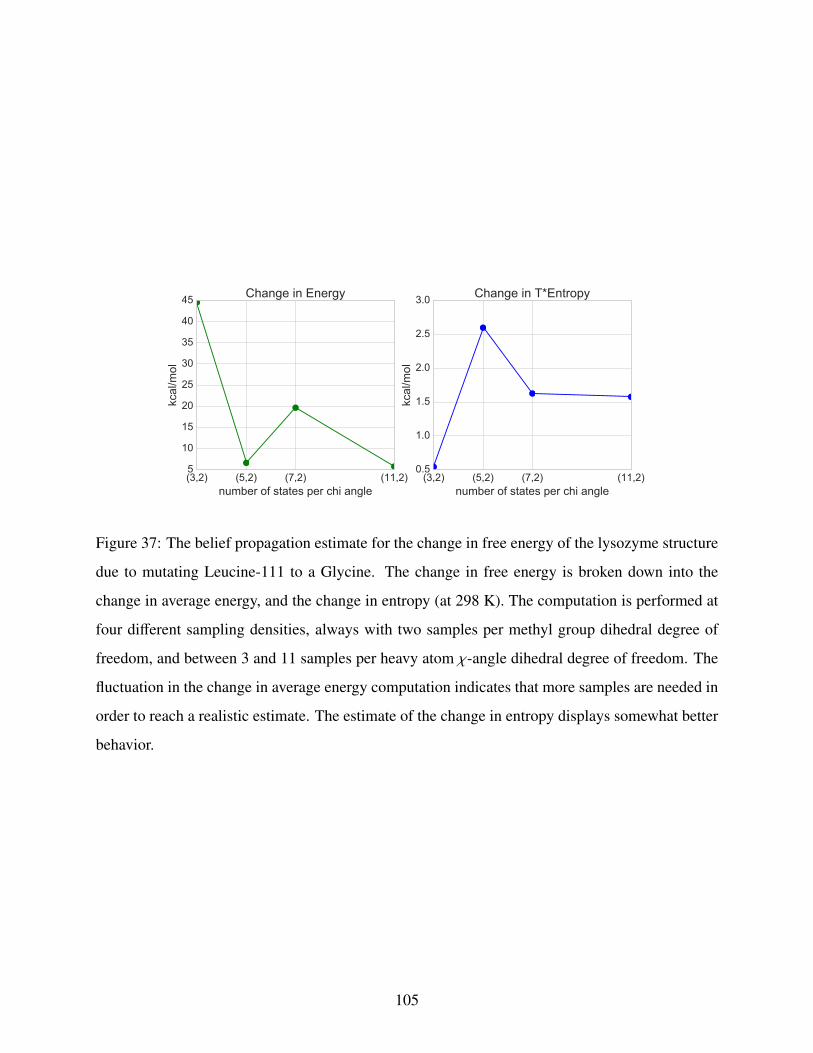
(3,2) (5,2) (7,2) (11,2)number of states per chi angle

5

10

15

20

25

30

35

40

45

kcal

/mol

Change in Energy

(3,2) (5,2) (7,2) (11,2)number of states per chi angle

0.5

1.0

1.5

2.0

2.5

3.0

kcal

/mol

Change in T*Entropy

Figure 37: The belief propagation estimate for the change in free energy of the lysozyme structure

due to mutating Leucine-111 to a Glycine. The change in free energy is broken down into the

change in average energy, and the change in entropy (at 298 K). The computation is performed at

four different sampling densities, always with two samples per methyl group dihedral degree of

freedom, and between 3 and 11 samples per heavy atom χ-angle dihedral degree of freedom. The

fluctuation in the change in average energy computation indicates that more samples are needed in

order to reach a realistic estimate. The estimate of the change in entropy displays somewhat better

behavior.

105

mated change in entropy does show some signs of converging, though further sampling would be

necessary to confirm this.

4.6.5 Future Work

There are many facets of this work that could be improved or expanded upon. Most practically, the

current bottleneck in estimating free energies using Markov random fields is the generation of the

Markov random fields themselves. My pipeline uses OpenMM to calculate the interaction energies

for the node and edge potentials This library is remarkably flexible, but the Python interface by

which I access the energetics information is quite slow compared to state of the art lower-level

implementations such as those used in molecular dynamics packages or as implemented in [57].

At the level of sampling used here, this bottleneck is a practical hurdle, not a theoretical one, and

there is no reason that implementing a more efficient graph generation pipeline could not result in

large speedups in the time expended generating the Markov random fields. Related to speeding

up the graph generation process is improving it in quality. The solvent model for the graphs is

currently a simple uniform relative dielectric constant of 60.0. While most sophisticated solvent

models have difficulty being decomposed into single or pairwise residue components, there is

definitely room for improvement in this regard.

Even if generating the Markov random field is not slow enough to be the main bottleneck

in the process, at some point the number of states sampled will be too large to hold in memory

and perform computations with. This motivates the thought that instead of uniformly sampling

states in dihedral space, one could be more be more selective in both generating and retaining

samples. States that are explicit clashes and have effectively zero probability of occurring could

be pruned away, saving a significant fraction of space. Additionally, one could consider sampling

the dihedral degrees of freedom at different densities, depending on their relative importance in

generating large conformational changes in the side-chain. That is, the χ1 angles might be sampled

at a higher density that the χ2 angles, with coarser sampling as one moves down the side-chain.

Further reduction in MRF complexity could be achieved by making more extensive use of nodes

with singleton, or otherwise severely reduced state-spaces, employed for portions of the structure

one has less interest in studying.

106

More radically, one could consider abandoning uniform sampling, and attempt to use, say, a

Boltzmann sampled ensemble of states for the nodes. This approach would require very careful

attention to weighting the samples, as it is quite easy to arrive at an incorrect estimate of the

partition function when the states account for different proportions of state space. For instance, the

logarithmic correction of equation A.24 is no longer entirely accurate, as the states no longer evenly

divide up the volume of state space. The advantage to a “hands-off” approach like Boltzmann

sampling is appealing though, as it would allow one to include arbitrary degrees of freedom in the

samples, and it would be worth investigating.

Lastly, throughout this exploratory work, we have used a fixed backbone in all of the systems.

To accurately capture the physics of the system these degrees of freedom need to be incorporated.

Drawing samples from a backbone ensemble, and generating graphs for each backbone, as in [57]

is an option. Another approach that would account for small flexing motions would be to include

in the nodes some amount of flexibility in the backbone degrees of freedom, but not enough to

alter the topology of the graph. This would expand the size of the node and edge potentials by

a multiplicative factor, so the benefit of doing so would have to be weighed against the cost of

generating a larger Markov random field.

4.7 SUMMARY

The goal of this investigation was to explore the performance of belief propagation approximations

of the free energy of Markov random fields constructed using the energetic interactions of peptides

and proteins, both compared to exact methods on fixed MRFs and in a self-consistent manner as the

sampling density of the MRF is increased. In the regime where belief propagation can be compared

to an exact brute-force result (small peptides), the belief propagation result agreed with brute-force

to a tremendous degree. In larger systems where brute-force approaches fail and a polymer growth

estimate must be used as a point of comparison (lysozyme binding pocket and surrogate peptide),

the belief propagation estimate is within the fairly tight bounds of the converged polymer growth

estimates. In the smaller test systems, it was found that increasing the sampling density to anything

above three states per dihedral degree of freedom significantly improved the convergence of the

107

belief propagation free energy estimates. In larger systems, the situation was more complicated:

while BP estimates agreed with polymer growth’s exact computations, convergence of the MRFs

themselves was unclear, perhaps implying that denser samples are necessary in such situations. In

both large and small systems, the belief propagation algorithm takes about a second to compute

its estimates, while the brute force and polymer growth estimates take anywhere from hours to

days to run. While this is not conclusive proof that belief propagation is always the best method

to compute free energies in Markov random fields modeling protein structures, the performance

of belief propagation was observed to be impressively accurate compared to exact methods in a

nontrivial set of examples.

108

5.0 CONCLUSIONS

While computational models of biological processes can be incredibly useful tools, unfortunately,

most useful models are slow. The unifying theme of this work has been an interest in the expansion

of the realm of computationally feasibility in biological simulation. To this end, I have studied two

distinct approaches that can be used to more efficiently sample complex biological simulations.

The weighted ensemble methodology is a fairly “hands-off” approach that is agnostic to the

nature of the simulation. The efficacy of weighted ensemble sampling in complex models opens the

door to integrating genomic-scale data into dynamical systems models. The flexibility of weighted

ensemble sampling is also lends itself to simulating models containing processes at different physi-

cal scales, and of diverse types. While parameterizing such models will require care, it is no longer

unthinkable that it is possible to simulate a stochastic simulation of cell scale processes in detail.

The flexibility of weighted ensemble contrasts strikingly with Markov random fields, which

place strong constraints on the structure of the models that can be studied in their formalism.

Within their scope, these highly structured models, when coupled with appropriate algorithms,

yield otherwise difficult to obtain information at high efficiency. In a way, this is because they are

not actually “simulating” anything, in the sense of propagating dynamics. In the creation of the

Markov random field, one pre-computes a subset of interactions, and use this cached information to

infer the result. Because there are no time-correlations to overcome, as in molecular dynamics, this

trade-off of a higher memory footprint for a lower run-time turns out to be immensely beneficial

in many cases. It has been known for some time that belief propagation on Markov random fields

presents a powerful tool for estimating free energies in bimolecular systems [54, 57]. This present

work contributes some small further confirmations of this fact, and presents some evidence that

these estimates could be further improved by slightly denser sampling of the side-chain state-

space.

109

While different in nature, both formalisms yield impressive increases in the efficiency of infer-

ring biologically relevant observables. It is hoped that the small gains detailed herein will facilitate

the construction of characterization of more detailed and accurate models, and a more comprehen-

sive and integrated study of complex biological systems in general.

110

APPENDIX A

CORRECTING FOR DISCRETIZATION IN PARTITION FUNCTION ESTIMATES

A.1 DERIVING THE EXACT FORMULA FOR ENTROPY

We start with the standard definition of the free energy:

F = 〈E〉 − TS =⇒ S/kB = βTS = −βF + β 〈E〉 (A.1)

= log Z +⟨βE

⟩(A.2)

= log(Z/V0

)+

⟨βE

⟩(A.3)

where β = 1/kBT is the inverse temperature, and the partition function Z has been decomposed into

the configurational partition function Z and a volume factor V0 corresponding to the momentum-

space partition function and suitable factors of ~. The configurational partition function is an

integral over all positional degrees of freedom, and as such has dimensions of volume, while the

factor V0, which also has dimensions of volume, makes the quotient Z/V0 appropriately dimen-

sionless. This volume factor can further be decomposed into a product of thermal wavelengths, as

in [115], but I leave it as an essentially arbitrary fiducial volume whose role is to keep the units of

the logarithm correctly dimensionless, since (as we will see) the precise value of V0 will cancel in

any physically relevant calculation, which involves taking a difference of free energies.

We will now focus on the second term in the expression for S/kB, the expectation of βE.

Employing the definition of the normalized probability in terms of the Boltzmann factor of the

111

energy, we can manipulate the expression to isolate the energy term:

ρ(x) =1Z

e−βE(x) (A.4)

⇐⇒ βE(x) = − log(ρ(x)Z

)(A.5)

= − log(V0

V0ρ(x)Z

)(A.6)

= −(log

(Z/V0

)+ log

(ρ(x)V0

))(A.7)

where this time I have introduced V0 entirely artificially, for the sake of keeping the units in the

argument of the logarithms dimensionless. Plugging this result into the formal definition of expec-

tation with respect to a probability distribution, over all coordinates x, we have

⟨βE

⟩=

∫

Vρ(x)βE(x)dx (A.8)

= −∫

Vρ(x)

(log

(Z/V0

)+ log

(ρ(x)V0

))dx (A.9)

= −(log

(Z/V0

) ∫

Vρ(x)dx +

∫

Vρ(x) log

(ρ(x)V0

)dx

)(A.10)

= −(log

(Z/V0

)+

∫

Vρ(x) log

(ρ(x)V0

)dx

)(A.11)

where the first integral in equation A.10 goes to unity by the normalization of ρ(x).

We can now substitute this expression for⟨βE

⟩into our original expression for the entropy:

S/kB = log(Z/V0

)+

⟨βE

⟩(A.12)

= log(Z/V0

)−

(log

(Z/V0

)+

∫

Vρ(x) log

(ρ(x)V0

)dx

)(A.13)

= −∫

Vρ(x) log

(ρ(x)V0

)dx (A.14)

This equation for the entropy is starting to resemble “that awful∑

p log p formula” [115] formula,

but some further manipulations are needed before it’s of use in a discretely sampled space.

112

A.2 DISCRETIZING THE EXACT ENTROPY FORMULA

To discretize the entropy formula so that it is applicable when dealing with a finite number of

samples, we approximate it by a Riemann sum:

S/kB = −∫

Vρ(xi) log

(ρ(x)V0

)dx (A.15)

≈ −N∑

i

ρ(xi) log(ρ(x)V0

)∆xi (A.16)

where the equality holds as N → ∞ and all ∆xi → 0. Note that N here is the number of rectangles

in the integral, and not the usual statistical mechanics usage of the number of particles in a system.

When using a finite number of samples to represent a distribution, the probability of each

sample pi (that you might get from e.g. a marginal probability in belief propagation) is related to

the probability density ρ by pi = ρ(xi)∆xi. That is, the area of a rectangle (in the Riemann sum) is

equal to its width times its height. Of course ∆xi here is not just one dimensional, but an arbitrarily

dimensioned sub-volume of configuration space. Substituting in, we get

S/kB = −N∑

i

(

pi

∆xi

)log

(pi

∆xiV0

) ∆xi (A.17)

= −N∑

i

pi log(

pi

∆xiV0

)(A.18)

= −N∑

i

pi log pi −N∑

i

pi logV0

∆xi(A.19)

For a uniform discretization, ∆x = V/N, so

S/kB = −N∑

i

pi log pi −N∑

i

pi logV0

V/N(A.20)

= −N∑

i

pi log pi − logV0

V/N

N∑

i

pi (A.21)

= −N∑

i

pi log pi − logV0

V/N(A.22)

= −N∑

i

pi log pi − logN

V/V0(A.23)

= −N∑

i

pi log pi − log N + log V/V0 (A.24)

113

So we see the logarithmic correction term(− log N

), as used in e.g. [57] for discretizing a con-

tinuous system, emerge naturally from a statistical physics treatment of the problem – it’s just

accounting for bin widths when translating from an integral to a Riemann sum. Lastly, we note

that the constant term, log V/V0, will cancel when computing entropy differences, for example the

change in entropy upon binding, even when using entropies computed using a different number of

states.

A.3 CORRECTIONS FOR Z AND F, BUT NOT E

Similarly, we must correct computations of the configurational partition function Z when approxi-

mating it using a finite number of samples:

Z =

∫

Ve−βE(x)dx (A.25)

≈N∑

i

e−βE(xi)∆xi (A.26)

where the sum becomes exact in the limit N → ∞ and all xi → 0. If we use a uniform spatial grid,

∆xi = ∆x = VN is a constant, and we can factor it out of the sum:

Z =VN

N∑

i

e−βE(xi) (A.27)

Where again, it is useful to think of e−βE(xi)∆x as the area of a box in a Riemann sum.

We can transform into the free-energy picture, using Z = Z/V0 = e−βF:

F = −1β

log(Z/V0

)(A.28)

= −1β

log

V/V0

N

N∑

i

e−βE(xi)

(A.29)

= −1β

log

N∑

i

e−βE(xi)

+1β

logN

V/V0(A.30)

= −1β

log

N∑

i

e−βE(xi)

+1β

log N − 1β

log (V/V0) (A.31)

114

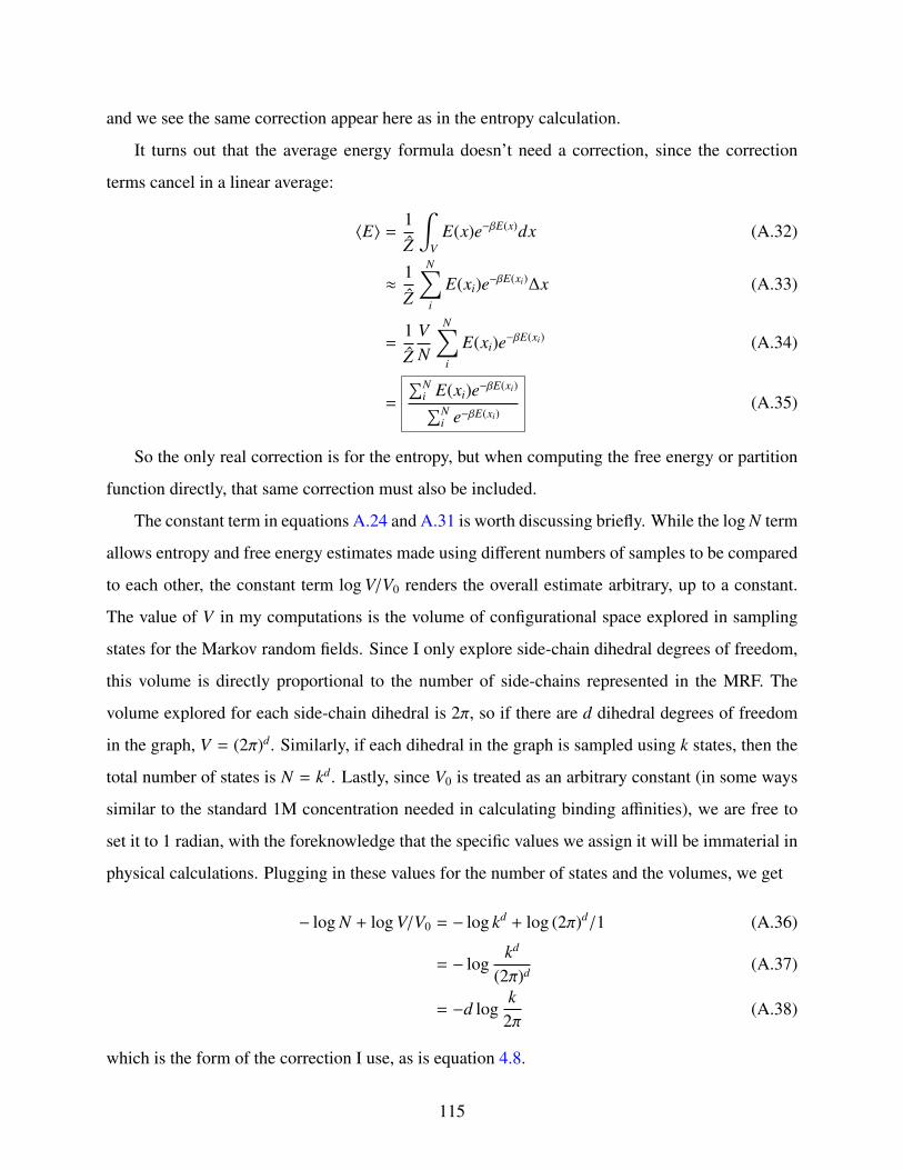
and we see the same correction appear here as in the entropy calculation.

It turns out that the average energy formula doesn’t need a correction, since the correction

terms cancel in a linear average:

〈E〉 =1Z

∫

VE(x)e−βE(x)dx (A.32)

≈ 1Z

N∑

i

E(xi)e−βE(xi)∆x (A.33)

=1Z

VN

N∑

i

E(xi)e−βE(xi) (A.34)

=

∑Ni E(xi)e−βE(xi)

∑Ni e−βE(xi)

(A.35)

So the only real correction is for the entropy, but when computing the free energy or partition

function directly, that same correction must also be included.

The constant term in equations A.24 and A.31 is worth discussing briefly. While the log N term

allows entropy and free energy estimates made using different numbers of samples to be compared

to each other, the constant term log V/V0 renders the overall estimate arbitrary, up to a constant.

The value of V in my computations is the volume of configurational space explored in sampling

states for the Markov random fields. Since I only explore side-chain dihedral degrees of freedom,

this volume is directly proportional to the number of side-chains represented in the MRF. The

volume explored for each side-chain dihedral is 2π, so if there are d dihedral degrees of freedom

in the graph, V = (2π)d. Similarly, if each dihedral in the graph is sampled using k states, then the

total number of states is N = kd. Lastly, since V0 is treated as an arbitrary constant (in some ways

similar to the standard 1M concentration needed in calculating binding affinities), we are free to

set it to 1 radian, with the foreknowledge that the specific values we assign it will be immaterial in

physical calculations. Plugging in these values for the number of states and the volumes, we get

− log N + log V/V0 = − log kd + log (2π)d/1 (A.36)

= − logkd

(2π)d (A.37)

= −d logk

2π(A.38)

which is the form of the correction I use, as is equation 4.8.

115

As a last note, it is worth drawing attention to the negative entropy values that appear at times

in the figures in this work. These negative values are solely the result of my choice of 1 radian for

V0, and do not reflect any sort of spooky physics going on. For instance, had I chosen 2π radians

instead of one, the entropies would all be positive, but since at the end of the day it is entropy

differences that matter, the choice of V0 only affects of the computation by way of numerical

stability. For this purpose, any number on the order of 2π is adequate.

116

APPENDIX B

UNIFORM SAMPLING COMPUTES THE CORRECT PARTITION FUNCTION

In constructing a Markov random field to approximate the free energies of biomolecules, there

is considerable freedom in choosing the state space of the model. An immediate simplification

is to only consider dihedral degrees of freedom in the side-chains of the amino acids, which is

what I have done in this work. In analyzing the correctness of partition function (or equivalently,

free energy) computations, it is simplest to ignore belief propagation or polymer growth or other

particular algorithms, and focus instead on brute-force computation, since all three converge on

the same answer, but brute-force is the simplest to reason about.

In fact, the simplest non-trivial model system to analyze is a graph with just one node, and

hence no edges. This one node graph represents a fixed-backbone peptide with one amino acid,

and let us further assume that the single side-chain has only one dihedral angle degree of freedom.

To find the free energy of the system, we then need only to apply the continuous analogue of the

definition of the partition function in equation 1.2 to our system:

Z =

∫ 2π

0e−βE(θ)dθ (B.1)

Since there is no Jacobian factor for the dihedral angle, uniform sampling over the state space

volume (V = [0, 2π)) is the proper way to construct the integral. A uniform discretization of this

integral yields

Z ≈ 2πN

N∑

i

e−βE(θi) (B.2)

Now consider the situation from the belief propagation point of view: if the states for the node

117

are sampled uniformly, and plugged in our Markov random field as usual, this is precisely the

(correct) answer we will get.

On the other hand, one might be tempted to sample according to, say, a Boltzmann distribution.

In this case, in plugging such states into a Markov random field and treating them as usual, we

would get the wrong answer. This is most easily illustrated in the integral formulation, where

the effect of the Boltzmann weighting of the states, ρ(θ), can be seen to induce a sort of double-

counting of the weights:

Zwrong =

∫ 2π

0e−βE(θ)ρ(θ)dθ

=

∫ 2π

0e−βE(θ) e−βE(θ)

Z(β)dθ

=1

Z(β)

∫e−2βE(θ)dθ

=Z(2β)Z(β)

It might be possible to correct for this effect, but the simple approach taken here is to eschew

sophisticated sampling techniques and use a uniform sampling of states.

118

APPENDIX C

CODE EXCERPTS

def brute_force_Z(graph):

all_var_inds = nx.get_node_attributes(graph, ’node_state_indices’)

all_node_pots = nx.get_node_attributes(graph, ’node_potential’)

all_edge_pots = nx.get_edge_attributes(graph, ’edge_potential’)

Z = 0.0

for global_state in it.product(*all_var_inds.itervalues()):

z = 0.0

z_node = 1.0

for node in graph.nodes_iter():

z_node *= all_node_pots[node][global_state[node], 0]

z_edge = 1.0

for edge in graph.edges_iter():

n_a, n_b = edge

z_edge *= all_edge_pots[edge][global_state[n_a]][global_state[n_b]]

z = z_node * z_edge

Z += z

return Z

Listing C.1: Brute Force Algorithm

def polymer_growth(graph, samples=100):

# initialize array of delta beta*F values

delta_betaF = np.zeros(len(g.nodes()))

# initialize ’polymer’: each state is a list, saved_states is a list of lists

saved_states = [[]]

saved_ens = [0.0]

119

# successively add each node, calculate delta F, and downsample

nodes = [n for n in g.nodes_iter()]

for node in nodes:

# h is a temp graph with nodes/edges > i removed

h = g.copy()

h.remove_nodes_from(nodes[node + 1:])

new_states = []

delta_ens = []

# check all the new states we get by adding in a new node to the old states

for node_state in h.node[node][’node_state_indices’]:

for i, old_state in enumerate(saved_states):

new_state = old_state + [node_state]

new_states.append(new_state)

new_en = get_betaU_for_state(h, new_state)

delta_en = new_en - saved_ens[i]

delta_ens.append(delta_en)

# compute tthe change in free energy

delta_betaF[node] = calc_betaF(delta_ens, len(saved_states))

# downsample according the the boltzmann factor of the change in F

saved_states = sample_states(new_states, delta_ens, samples=samples)

saved_ens = [get_betaU_for_state(h, state) for state in saved_states]

# after all the nodes are added and the graph is rebuilt, compute our stats:

betaF = np.sum(delta_betaF)

betaU = np.mean([get_betaU_for_state(h, state) for state in saved_states])

betaTS = betaU - betaF

return betaF, betaU, betaTS

Listing C.2: Polymer Growth Algorithm

def runBP(some_graph, N_BPiters=100, epsilon=1e-12):

deltas = []

converged = False

# initialize all messages as ones

new_messages, old_messages = initialize_messages(some_graph)

for N_BPiter in xrange(N_BPiters):

for node_from in some_graph.nodes_iter():

for node_to in some_graph.neighbors(node_from):

nodes_gather = [n for n in some_graph.neighbors(node_from) if n != node_to]

i, j = node_to, node_from

120

# start out with node potential as message;

# if no neighbors other than target node, this is what gets passed

x = copy.deepcopy(some_graph.node[j][’node_potential’])

# if the node passing the message only has one state, short circuit

# the message gathering etc, and just pass the 1x1 identity.

if x.shape == (1,1):

new_messages[j][i] = np.ones_like(x)

# if the node has neighbors, other than the receiving node, gather incoming

# messages to the sending node and ready a new message for the receiving node

else:

if nodes_gather:

for k in nodes_gather:

x *= old_messages[k][j] # messages are [from][to]

# hit node i’s info with the ij edge potential and pass to j

psi_ij = copy.deepcopy(some_graph.edge[i][j][’edge_potential’])

if j < i:

psi_ij = psi_ij.T

# messages are now col vectors

new_messages[j][i] = psi_ij.dot(x)

# normalize the new message

new_messages[j][i] = new_messages[j][i] / np.sum(new_messages[j][i])

# check for convergence

delta = compute_delta(old_messages, new_messages, verbose=verbose)

deltas.append(delta)

if delta < epsilon:

converged = True

break

# get ready for the next iteration of BP, if needed

old_messages = copy.deepcopy(new_messages)

node_beliefs = calculate_node_beliefs(some_graph, new_messages)

edge_beliefs = calculate_edge_beliefs(some_graph, new_messages)

return node_beliefs, edge_beliefs, new_messages, converged, deltas

Listing C.3: Belief Propagation Algorithm

121

BIBLIOGRAPHY

[1] Rory M Donovan, Andrew J Sedgewick, James R Faeder, and Daniel M Zuckerman. Ef-ficient stochastic simulation of chemical kinetics networks using a weighted ensemble oftrajectories. The Journal of chemical physics, 139(11):115105, September 2013.

[2] Manel Esteller. Epigenetics in cancer. The New England journal of medicine, 358(11):1148–59, March 2008.

[3] H H McAdams and A Arkin. Stochastic mechanisms in gene expression. Proceedings ofthe National Academy of Sciences of the United States of America, 94(3):814–9, February1997.

[4] A Arkin, J Ross, and H H McAdams. Stochastic kinetic analysis of developmental path-way bifurcation in phage lambda-infected Escherichia coli cells. Genetics, 149(4):1633–48,August 1998.

[5] William J Blake, Mads Kaern, Charles R Cantor, and J J Collins. Noise in eukaryotic geneexpression. Nature, 422(6932):633–7, April 2003.

[6] Jonathan M Raser and Erin K O’Shea. Control of stochasticity in eukaryotic gene expres-sion. Science (New York, N.Y.), 304(5678):1811–4, June 2004.

[7] Leor S Weinberger, John C Burnett, Jared E Toettcher, Adam P Arkin, and David V Schaffer.Stochastic gene expression in a lentiviral positive-feedback loop: HIV-1 Tat fluctuationsdrive phenotypic diversity. Cell, 122(2):169–82, July 2005.

[8] Murat Acar, Jerome T Mettetal, and Alexander van Oudenaarden. Stochastic switching as asurvival strategy in fluctuating environments. Nature genetics, 40(4):471–5, April 2008.

[9] Long Cai, Nir Friedman, and X Sunney Xie. Stochastic protein expression in individualcells at the single molecule level. Nature, 440(7082):358–62, March 2006.

[10] Michael B Elowitz, Arnold J Levine, Eric D Siggia, and Peter S Swain. Stochastic geneexpression in a single cell. Science, 297(5584):1183–6, August 2002.

[11] Arjun Raj and Alexander van Oudenaarden. Nature, nurture, or chance: stochastic geneexpression and its consequences. Cell, 135(2):216–26, October 2008.

122

[12] Narendra Maheshri and Erin K O’Shea. Living with noisy genes: how cells function reliablywith inherent variability in gene expression. Annual review of biophysics and biomolecularstructure, 36:413–34, January 2007.

[13] Benjamin B Kaufmann and Alexander van Oudenaarden. Stochastic gene expression: fromsingle molecules to the proteome. Current opinion in genetics & development, 17(2):107–12, April 2007.

[14] Vahid Shahrezaei and Peter S Swain. The stochastic nature of biochemical networks. Cur-rent opinion in biotechnology, 19(4):369–74, August 2008.

[15] Arjun Raj and Alexander van Oudenaarden. Single-molecule approaches to stochastic geneexpression. Annual review of biophysics, 38:255–70, January 2009.

[16] Daniel T Gillespie. Stochastic simulation of chemical kinetics. Annual review of physicalchemistry, 58:35–55, January 2007.

[17] Darren James Wilkinson. Stochastic Modelling for Systems Biology, Second Edition, volume2011. CRC Press, 2011.

[18] Michael L Blinov, James R Faeder, Byron Goldstein, and William S Hlavacek. BioNet-Gen: software for rule-based modeling of signal transduction based on the interactions ofmolecular domains. Bioinformatics (Oxford, England), 20(17):3289–91, November 2004.

[19] Daniel T Gillespie. A general method for numerically simulating the stochastic time evo-lution of coupled chemical reactions. Journal of Computational Physics, 22(4):403–434,December 1976.

[20] Daniel T. Gillespie. Exact stochastic simulation of coupled chemical reactions. The Journalof Physical Chemistry, 81(25):2340–2361, December 1977.

[21] Rosalind Allen, Patrick Warren, and Pieter ten Wolde. Sampling Rare Switching Events inBiochemical Networks. Physical Review Letters, 94(1):018104–, January 2005.

[22] Wen Zhou, Xinjun Peng, Zhenglou Yan, and Yifei Wang. Accelerated stochastic simulationalgorithm for coupled chemical reactions with delays. Computational biology and chem-istry, 32(4):240–2, August 2008.

[23] Eric Mjolsness, David Orendorff, Philippe Chatelain, and Petros Koumoutsakos. Anexact accelerated stochastic simulation algorithm. The Journal of chemical physics,130(14):144110, April 2009.

[24] David D. Jenkins and Gregory D. Peterson. AESS: Accelerated Exact Stochastic Simulation.Computer Physics Communications, 182(12):2580–2586, December 2011.

[25] Abhijit Chatterjee, Kapil Mayawala, Jeremy S Edwards, and Dionisios G Vlachos. Timeaccelerated Monte Carlo simulations of biological networks using the binomial tau-leapmethod. Bioinformatics (Oxford, England), 21(9):2136–7, May 2005.

123

[26] Basil Bayati, Philippe Chatelain, and Petros Koumoutsakos. D-leaping: Acceleratingstochastic simulation algorithms for reactions with delays. Journal of ComputationalPhysics, 228(16):5908–5916, September 2009.

[27] Daniel T. Gillespie and Linda R. Petzold. Improved leap-size selection for acceleratedstochastic simulation. The Journal of Chemical Physics, 119(16):8229, October 2003.

[28] Haokai Lu and Peng Li. Stochastic projective methods for simulating stiff chemical reactingsystems. Computer Physics Communications, 183(7):1427–1442, July 2012.

[29] Michael A. Gibson and Jehoshua Bruck. Efficient Exact Stochastic Simulation of ChemicalSystems with Many Species and Many Channels. The Journal of Physical Chemistry A,104(9):1876–1889, March 2000.

[30] Hiroyuki Kuwahara and Ivan Mura. An efficient and exact stochastic simulation methodto analyze rare events in biochemical systems. The Journal of chemical physics,129(16):165101, October 2008.

[31] Dan T Gillespie, Min Roh, and Linda R Petzold. Refining the weighted stochastic simulationalgorithm. The Journal of chemical physics, 130(17):174103, May 2009.

[32] Min K Roh, Dan T Gillespie, and Linda R Petzold. State-dependent biasing method for im-portance sampling in the weighted stochastic simulation algorithm. The Journal of chemicalphysics, 133(17):174106, November 2010.

[33] Bernie J Daigle, Min K Roh, Dan T Gillespie, and Linda R Petzold. Automated estima-tion of rare event probabilities in biochemical systems. The Journal of chemical physics,134(4):044110, January 2011.

[34] Min K Roh, Bernie J Daigle, Dan T Gillespie, and Linda R Petzold. State-dependent doublyweighted stochastic simulation algorithm for automatic characterization of stochastic bio-chemical rare events. The Journal of chemical physics, 135(23):234108, December 2011.

[35] Rosalind J Allen, Daan Frenkel, and Pieter Rein ten Wolde. Simulating rare eventsin equilibrium or nonequilibrium stochastic systems. The Journal of chemical physics,124(2):024102, January 2006.

[36] Rosalind J Allen, Daan Frenkel, and Pieter Rein ten Wolde. Forward flux sampling-typeschemes for simulating rare events: efficiency analysis. The Journal of chemical physics,124(19):194111, May 2006.

[37] Rosalind J Allen, Chantal Valeriani, and Pieter Rein ten Wolde. Forward flux sampling forrare event simulations. Journal of physics: Condensed matter, 21(46):463102, November2009.

[38] Alex Dickson, Aryeh Warmflash, and Aaron R Dinner. Nonequilibrium umbrella samplingin spaces of many order parameters. The Journal of chemical physics, 130(7):074104, Febru-ary 2009.

124

[39] Aryeh Warmflash, Prabhakar Bhimalapuram, and Aaron R Dinner. Umbrella sampling fornonequilibrium processes. The Journal of chemical physics, 127(15):154112, October 2007.

[40] Daniel M. Zuckerman and Thomas B. Woolf. Dynamic reaction paths and rates throughimportance-sampled stochastic dynamics. The Journal of Chemical Physics, 111(21):9475,December 1999.

[41] Anton K Faradjian and Ron Elber. Computing time scales from reaction coordinates bymilestoning. The Journal of chemical physics, 120(23):10880–9, June 2004.

[42] Christoph Dellago, Peter G. Bolhuis, FeÌAlix S. Csajka, and David Chandler. Transitionpath sampling and the calculation of rate constants. The Journal of Chemical Physics,108(5):1964, February 1998.

[43] Titus S. van Erp, Daniele Moroni, and Peter G. Bolhuis. A novel path sampling methodfor the calculation of rate constants. The Journal of Chemical Physics, 118(17):7762, May2003.

[44] G A Huber and S Kim. Weighted-ensemble Brownian dynamics simulations for proteinassociation reactions. Biophysical journal, 70(1):97–110, January 1996.

[45] Bin W Zhang, David Jasnow, and Daniel M Zuckerman. Efficient and verified simula-tion of a path ensemble for conformational change in a united-residue model of calmod-ulin. Proceedings of the National Academy of Sciences of the United States of America,104(46):18043–8, November 2007.

[46] Bin W Zhang, David Jasnow, and Daniel M Zuckerman. The "weighted ensemble" pathsampling method is statistically exact for a broad class of stochastic processes and binningprocedures. The Journal of chemical physics, 132(5):054107, February 2010.

[47] Divesh Bhatt, Bin W Zhang, and Daniel M Zuckerman. Steady-state simulations usingweighted ensemble path sampling. The Journal of chemical physics, 133(1):014110, July2010.

[48] Matthew C. Zwier, Joseph W. Kaus, and Lillian T. Chong. Efficient Explicit-Solvent Molec-ular Dynamics Simulations of Molecular Association Kinetics: Methane/Methane, Na + /ClâLŠ , Methane/Benzene, and K + /18-Crown-6 Ether. Journal of Chemical Theory andComputation, 7(4):1189–1197, April 2011.

[49] Joshua L Adelman and Michael Grabe. Simulating rare events using a weighted ensemble-based string method. The Journal of chemical physics, 138(4):044105, January 2013.

[50] Steven Lettieri, Matthew C. Zwier, Carsen A. Stringer, Ernesto Suarez, Lillian T. Chong,and Daniel M. Zuckerman. Simultaneous computation of dynamical and equilibrium infor-mation using a weighted ensemble of trajectories. e-print, October 2012.

[51] Matthew C Zwier, Joshua L Adelman, Joseph W Kaus, Adam J Pratt, Kim F Wong,Nicholas B Rego, Ernesto Suárez, Steven Lettieri, David W Wang, Michael Grabe, et al.

125

Westpa: An interoperable, highly scalable software package for weighted ensemble simula-tion and analysis. Journal of chemical theory and computation, 11(2):800–809, 2015.

[52] Matthew C Zwier and Lillian T Chong. Reaching biological timescales with all-atom molec-ular dynamics simulations. Current opinion in pharmacology, 10(6):745–52, December2010.

[53] James R Faeder, Michael L Blinov, and William S Hlavacek. Rule-based modeling of bio-chemical systems with BioNetGen. Methods in molecular biology, 500:113–67, January2009.

[54] H. Kamisetty, E.P. Xing, and C.J. Langmead. Free Energy Estimates of All-atom ProteinStructures Using Generalized Belief Propagation. J. Comp. Bio., 15(7):755–766, 2008.

[55] C.J. Kamisetty, H.and Langmead. Conformational Free Energy of Protein Structures: Com-puting Upper and Lower bounds. In Proc. Structural Bioinformatics and ComputationalBiophysics (3DSIG), pages 23–24, 2008.

[56] S. Balakrishnan, H. Kamisetty, J.C. Carbonell, S.I. Lee, and Langmead C.J. Learning Gen-erative Models for Protein Fold Families. Proteins: Structure, Function, and Bioinformatics,79(6):1061–1078, 2011.

[57] Hetunandan Kamisetty, Arvind Ramanathan, Chris Bailey-Kellogg, and Christopher JamesLangmead. Accounting for conformational entropy in predicting binding free energies ofprotein-protein interactions. Proteins, 79(2):444–62, February 2011.

[58] Narges Sharif Razavian, Hetunandan Kamisetty, and Christopher J Langmead. Learninggenerative models of molecular dynamics. BMC genomics, 13 Suppl 1(Suppl 1):S5, January2012.

[59] Narges Sharif Razavian. Continuous graphical models for static and dynamic distributions:Application to structural biology. Ph.D. Dissertation, Carnegie Mellon University, 2013.

[60] Christopher James Langmead. Generative Models of Conformational Dynamics, pages 87–105. Springer International Publishing, Cham, 2014.

[61] Hetunandan Kamisetty, Bornika Ghosh, Christopher James Langmead, and Chris Bailey-Kellogg. Learning sequence determinants of protein: Protein interaction specificity withsparse graphical models. Journal of Computational Biology, 22(6):474–486, 2015.

[62] Huan-Xiang Zhou and Michael K Gilson. Theory of free energy and entropy in noncovalentbinding. Chemical reviews, 109(9):4092–4107, 2009.

[63] Michael K Gilson and Huan-Xiang Zhou. Calculation of protein-ligand binding affinities*.Annual review of biophysics and biomolecular structure, 36(1):21, 2007.

126

[64] Kevin P Murphy, Yair Weiss, and Michael I Jordan. Loopy belief propagation for approxi-mate inference: An empirical study. In Proceedings of the Fifteenth conference on Uncer-tainty in artificial intelligence, pages 467–475. Morgan Kaufmann Publishers Inc., 1999.

[65] Sekhar C Tatikonda and Michael I Jordan. Loopy belief propagation and gibbs measures.In Proceedings of the Eighteenth conference on Uncertainty in artificial intelligence, pages493–500. Morgan Kaufmann Publishers Inc., 2002.

[66] Martin J Wainwright, Tommi S Jaakkola, and Alan S Willsky. A new class of upper boundson the log partition function. IEEE Transactions on Information Theory, 51(7):2313–2335,2005.

[67] Joris M Mooij and Hilbert J Kappen. Sufficient conditions for convergence of the sum–product algorithm. IEEE Transactions on Information Theory, 53(12):4422–4437, 2007.

[68] Sekhar C Tatikonda. Convergence of the sum-product algorithm. In Information TheoryWorkshop, 2003. Proceedings. 2003 IEEE, pages 222–225. IEEE, 2003.

[69] Steffen L Lauritzen. Graphical models, volume 17. Clarendon Press, 1996.

[70] Michael Irwin Jordan. Learning in graphical models, volume 89. Springer Science &Business Media, 1998.

[71] Martin J Wainwright and Michael I Jordan. Graphical models, exponential families, andvariational inference. Foundations and Trends® in Machine Learning, 1(1-2):1–305, 2008.

[72] Daphne Koller and Nir Friedman. Probabilistic graphical models: principles and tech-niques. MIT press, 2009.

[73] Ross Kindermann and J. Laurie Snell. Markov Random Fields and Their Applications,volume 1 of Contemporary Mathematics. American Mathematical Society, Providence,Rhode Island, 1980.

[74] J.S. Yedidia, W.T. Freeman, and Y. Weiss. Constructing Free-Energy Approximations andGeneralized Belief Propagation Algorithms. IEEE Transactions on Information Theory,51(7):2282–2312, July 2005.

[75] Nils B Becker, Rosalind J Allen, and Pieter Rein ten Wolde. Non-stationary forward fluxsampling. The Journal of chemical physics, 136(17):174118, May 2012.

[76] Nils B. Becker and Pieter Rein ten Wolde. Rare switching events in non-stationary systems.e-print, January 2012.

[77] Ambarish Nag, Michael I Monine, James R Faeder, and Byron Goldstein. Aggregation ofmembrane proteins by cytosolic cross-linkers: theory and simulation of the LAT-Grb2-SOS1system. Biophysical journal, 96(7):2604–23, April 2009.

127

[78] Ofer Feinerman, Garrit Jentsch, Karen E Tkach, Jesse W Coward, Matthew M Hathorn,Michael W Sneddon, Thierry Emonet, Kendall A Smith, and Grégoire Altan-Bonnet.Single-cell quantification of IL-2 response by effector and regulatory T cells reveals crit-ical plasticity in immune response. Molecular systems biology, 6:437, November 2010.

[79] Haijun Gong, Paolo Zuliani, Anvesh Komuravelli, James R Faeder, and Edmund M Clarke.Analysis and verification of the HMGB1 signaling pathway. BMC bioinformatics, 11 Suppl7:S10, January 2010.

[80] Ty M Thomson, Kirsten R Benjamin, Alan Bush, Tonya Love, David Pincus, OrnaResnekov, Richard C Yu, Andrew Gordon, Alejandro Colman-Lerner, Drew Endy, andRoger Brent. Scaffold number in yeast signaling system sets tradeoff between system outputand dynamic range. Proceedings of the National Academy of Sciences of the United Statesof America, 108(50):20265–70, December 2011.

[81] Dipak Barua, William S Hlavacek, and Tomasz Lipniacki. A computational model for earlyevents in B cell antigen receptor signaling: analysis of the roles of Lyn and Fyn. Journal ofimmunology, 189(2):646–58, July 2012.

[82] Terrell L. Hill. Free Energy Transduction And Biochemical Cycle Kinetics. Dover Publica-tions, 2004.

[83] Bojan Zagrovic and Vijay Pande. Solvent viscosity dependence of the folding rate of a smallprotein: distributed computing study. Journal of computational chemistry, 24(12):1432–6,September 2003.

[84] Michael Samoilov, Sergey Plyasunov, and Adam P Arkin. Stochastic amplification andsignaling in enzymatic futile cycles through noise-induced bistability with oscillations. Pro-ceedings of the National Academy of Sciences of the United States of America, 102(7):2310–5, February 2005.

[85] Aryeh Warmflash, David N Adamson, and Aaron R Dinner. How noise statistics impactmodels of enzyme cycles. The Journal of chemical physics, 128(22):225101, June 2008.

[86] Boris N Kholodenko. Cell-signalling dynamics in time and space. Nature reviews. Molecu-lar cell biology, 7(3):165–76, March 2006.

[87] Liming Wang and Eduardo D Sontag. On the number of steady states in a multiple futilecycle. Journal of mathematical biology, 57(1):29–52, July 2008.

[88] F. Schlögl. Chemical reaction models for non-equilibrium phase transitions. Zeitschrift fürPhysik, 253(2):147–161, April 1972.

[89] Daniel T. Gillespie. Markov Processes: An Introduction for Physical Scientists. Gulf Pro-fessional Publishing, 1992.

128

[90] Melissa Vellela and Hong Qian. Stochastic dynamics and non-equilibrium thermodynamicsof a bistable chemical system: the Schlögl model revisited. Journal of the Royal Society,Interface / the Royal Society, 6(39):925–40, October 2009.

[91] David Roma, Ruadhan O’Flanagan, Andrei Ruckenstein, Anirvan Sengupta, and RanjanMukhopadhyay. Optimal path to epigenetic switching. Physical Review E, 71(1):011902,January 2005.

[92] Rory Donovan. Supplementary Material.

[93] James R. Faeder, William S. Hlavacek, Ilona Reischl, Michael L. Blinov, Henry Metzger,Antonio Redondo, Carla Wofsy, and Byron Goldstein. Investigation of Early Events inFc{epsilon}RI-Mediated Signaling Using a Detailed Mathematical Model. J. Immunol.,170(7):3769–3781, April 2003.

[94] Weinan E, Weiqing Ren, and Eric Vanden-Eijnden. Transition pathways in complex systems:Reaction coordinates, isocommittor surfaces, and transition tubes. Chemical Physics Letters,413(1-3):242–247, September 2005.

[95] Peter G Bolhuis, David Chandler, Christoph Dellago, and Phillip L Geissler. Transitionpath sampling: throwing ropes over rough mountain passes, in the dark. Annual review ofphysical chemistry, 53:291–318, January 2002.

[96] A Sali, E Shakhnovich, and M Karplus. How does a protein fold? Nature, 369(6477):248–51, May 1994.

[97] Ken A. Dill and Hue Sun Chan. From Levinthal to pathways to funnels. Nature StructuralBiology, 4(1):10–19, January 1997.

[98] Divesh Bhatt and Ivet Bahar. An adaptive weighted ensemble procedure for efficientcomputation of free energies and first passage rates. The Journal of chemical physics,137(10):104101, September 2012.

[99] Daniel M. Zuckerman and Thomas B. Woolf. Transition events in butane simulations: Sim-ilarities across models. The Journal of Chemical Physics, 116(6):2586, February 2002.

[100] Bin W Zhang, David Jasnow, and Daniel M Zuckerman. Transition-event durations in one-dimensional activated processes. The Journal of chemical physics, 126(7):074504, February2007.

[101] JR Stiles and TM Bartol. Computational neuroscience: Realistic modeling for experimen-talists. In E De Schutter, editor, Computational Neuroscience: Realistic Modeling for Ex-perimentalists, chapter Monte Carl, pages 87–127. CRC Press, Boca Raton, 2001.

[102] Rex A Kerr, Thomas M Bartol, Boris Kaminsky, Markus Dittrich, Jen-Chien Jack Chang,Scott B Baden, Terrence J Sejnowski, and Joel R Stiles. FAST MONTE CARLO SIMULA-TION METHODS FOR BIOLOGICAL REACTION-DIFFUSION SYSTEMS IN SOLU-

129

TION AND ON SURFACES. SIAM journal on scientific computing, 30(6):3126, October2008.

[103] J R Stiles, D Van Helden, T M Bartol, E E Salpeter, and M M Salpeter. Miniature end-plate current rise times less than 100 microseconds from improved dual recordings can bemodeled with passive acetylcholine diffusion from a synaptic vesicle. Proceedings of theNational Academy of Sciences of the United States of America, 93(12):5747–52, June 1996.

[104] Steven S Andrews. Spatial and stochastic cellular modeling with the Smoldyn simulator.Methods in molecular biology, 804:519–42, January 2012.

[105] Leonard A Harris and Paulette Clancy. A "partitioned leaping" approach for multiscalemodeling of chemical reaction dynamics. The Journal of chemical physics, 125(14):144107,October 2006.

[106] Tianhai Tian and Kevin Burrage. Binomial leap methods for simulating stochastic chemicalkinetics. The Journal of chemical physics, 121(21):10356–64, December 2004.

[107] Yang Cao, Daniel T Gillespie, and Linda R Petzold. Efficient step size selection for thetau-leaping simulation method. The Journal of chemical physics, 124(4):044109, January2006.

[108] Daniel T. Gillespie. Approximate accelerated stochastic simulation of chemically reactingsystems. The Journal of Chemical Physics, 115(4):1716, July 2001.

[109] Ulrich H.E. Hansmann. Parallel tempering algorithm for conformational studies of biologi-cal molecules. Chemical Physics Letters, 281(1-3):140–150, December 1997.

[110] Yuji Sugita and Yuko Okamoto. Replica-exchange molecular dynamics method for proteinfolding. Chemical Physics Letters, 314(1-2):141–151, November 1999.

[111] David J. Earl and Michael W. Deem. Parallel tempering: Theory, applications, and newperspectives. Physical Chemistry Chemical Physics, 7(23):3910, November 2005.

[112] Edmund M. Clarke, Orna Grumberg, and Doron A. Peled. Model Cheking. MIT Press,1999.

[113] Edmund M. Clarke, James R. Faeder, Christopher J. Langmead, Leonard A. Harris,Sumit Kumar Jha, and Axel Legay. Statistical Model Checking in BioLab: Applicationsto the Automated Analysis of T-Cell Receptor Signaling Pathway. Computational Methodsin Systems Biology, 5307:231–250, 2008.

[114] Sumit K. Jha, Edmund M. Clarke, Christopher J. Langmead, Axel Legay, Andre Platzer,and Paolo Zuliani. A Bayesian Approach to Model Checking Biological Systems. Compu-tational Methods in Systems Biology, 5688:218–234, 2009.

[115] D.M. Zuckerman. Statistical Physics of Biomolecules: An Introduction. Taylor & Francis,2010.

130

[116] Brian Munsky, Gregor Neuert, and Alexander van Oudenaarden. Using gene expressionnoise to understand gene regulation. Science, 336(6078):183–7, April 2012.

[117] Melanie I Stefan, Thomas M Bartol, Terrence J Sejnowski, and Mary B Kennedy. Multi-state modeling of biomolecules. PLoS computational biology, 10(9):e1003844, September2014.

[118] David E. Shaw, J.P. Grossman, Joseph A. Bank, Brannon Batson, J. Adam Butts, Jack C.Chao, Martin M. Deneroff, Ron O. Dror, Amos Even, Christopher H. Fenton, AnthonyForte, Joseph Gagliardo, Gennette Gill, Brian Greskamp, C. Richard Ho, Douglas J. Ier-ardi, Lev Iserovich, Jeffrey S. Kuskin, Richard H. Larson, Timothy Layman, Li-Siang Lee,Adam K. Lerer, Chester Li, Daniel Killebrew, Kenneth M. Mackenzie, Shark Yeuk-HaiMok, Mark A. Moraes, Rolf Mueller, Lawrence J. Nociolo, Jon L. Peticolas, Terry Quan,Daniel Ramot, John K. Salmon, Daniele P. Scarpazza, U. Ben Schafer, Naseer Siddique,Christopher W. Snyder, Jochen Spengler, Ping Tak Peter Tang, Michael Theobald, HoriaToma, Brian Towles, Benjamin Vitale, Stanley C. Wang, and Cliff Young. Anton 2: Raisingthe Bar for Performance and Programmability in a Special-Purpose Molecular DynamicsSupercomputer. In SC14: International Conference for High Performance Computing, Net-working, Storage and Analysis, pages 41–53. IEEE, November 2014.

[119] Ron O Dror, Robert M Dirks, J P Grossman, Huafeng Xu, and David E Shaw. Biomolecularsimulation: a computational microscope for molecular biology. Annual review of biophysics,41:429–52, January 2012.

[120] Jonathan R Karr, Jayodita C Sanghvi, Derek N Macklin, Miriam V Gutschow, Jared MJacobs, Benjamin Bolival, Nacyra Assad-Garcia, John I Glass, and Markus W Covert. Awhole-cell computational model predicts phenotype from genotype. Cell, 150(2):389–401,July 2012.

[121] G.M. Torrie and J.P. Valleau. Nonphysical sampling distributions in Monte Carlo free-energy estimation: Umbrella sampling. Journal of Computational Physics, 23(2):187–199,February 1977.

[122] Shankar Kumar, John M. Rosenberg, Djamal Bouzida, Robert H. Swendsen, and Pe-ter A. Kollman. THE weighted histogram analysis method for free-energy calculations onbiomolecules. I. The method. Journal of Computational Chemistry, 13(8):1011–1021, Oc-tober 1992.

[123] Giovanni Bussi, Alessandro Laio, and Michele Parrinello. Equilibrium Free Energies fromNonequilibrium Metadynamics. Physical Review Letters, 96(9):090601, March 2006.

[124] Daniele Moroni, Titus S. van Erp, and Peter G. Bolhuis. Investigating rare events by tran-sition interface sampling. Physica A: Statistical Mechanics and its Applications, 340(1-3):395–401, September 2004.

[125] Robert H. Swendsen and Jian-Sheng Wang. Replica Monte Carlo Simulation of Spin-Glasses. Physical Review Letters, 57(21):2607–2609, November 1986.

131

[126] Edward Lyman, F. Marty Ytreberg, and Daniel M. Zuckerman. Resolution Exchange Simu-lation. Physical Review Letters, 96(2):028105, January 2006.

[127] Harold A Scheraga, Mey Khalili, and Adam Liwo. Protein-folding dynamics: overview ofmolecular simulation techniques. Annual review of physical chemistry, 58:57–83, January2007.

[128] Daniel M Zuckerman. Equilibrium sampling in biomolecular simulations. Annual review ofbiophysics, 40:41–62, January 2011.

[129] Divesh Bhatt and Daniel M Zuckerman. Heterogeneous path ensembles for conformationaltransitions in semi-atomistic models of adenylate kinase. Journal of chemical theory andcomputation, 6(11):3527–3539, October 2010.

[130] Ernesto Suárez, Steven Lettieri, Matthew C. Zwier, Carsen A. Stringer, Sundar Raman Sub-ramanian, Lillian T. Chong, and Daniel M. Zuckerman. Simultaneous Computation of Dy-namical and Equilibrium Information Using a Weighted Ensemble of Trajectories. Journalof Chemical Theory and Computation, 10(7):2658–2667, July 2014.

[131] Markus Dittrich, John M Pattillo, J Darwin King, Soyoun Cho, Joel R Stiles, and Stephen DMeriney. An excess-calcium-binding-site model predicts neurotransmitter release at theneuromuscular junction. Biophysical journal, 104(12):2751–63, June 2013.

[132] Michael W Sneddon, James R Faeder, and Thierry Emonet. Efficient modeling, simulationand coarse-graining of biological complexity with NFsim. Nature methods, 8(2):177–83,February 2011.

[133] Won-Ki Huh, James V Falvo, Luke C Gerke, Adam S Carroll, Russell W Howson,Jonathan S Weissman, and Erin K O’Shea. Global analysis of protein localization in buddingyeast. Nature, 425(6959):686–91, October 2003.

[134] Josefine Sprenger, J Lynn Fink, Seetha Karunaratne, Kelly Hanson, Nicholas A Hamilton,and Rohan D Teasdale. LOCATE: a mammalian protein subcellular localization database.Nucleic acids research, 36(Database issue):D230–3, January 2008.

[135] L. P. Coelho, J. D. Kangas, A. W. Naik, E. Osuna-Highley, E. Glory-Afshar, M. Fuhrman,R. Simha, P. B. Berget, J. W. Jarvik, and R. F. Murphy. Determining the subcellular locationof new proteins from microscope images using local features. Bioinformatics, 29(18):2343–2349, July 2013.

[136] Matthew C. Zwier, Joshua Adelman, Joseph W. Kaus, Adam J. Pratt, Kim F. Wong,Nicholas B. Rego, Ernesto Suárez, Steven Lettieri, David W. Wang, Michael Grabe,Daniel M Zuckerman, and Lillian T. Chong. WESTPA: An interoperable, highly scalablesoftware package for weighted ensemble simulation and analysis. Journal of Chemical The-ory and Computation, 11(2):150113180903008, January 2015.

132

[137] Justin P. Kinney, Josef Spacek, Thomas M. Bartol, Chandrajit L. Bajaj, Kristen M. Harris,and Terrence J. Sejnowski. Extracellular sheets and tunnels modulate glutamate diffusion inhippocampal neuropil. Journal of Comparative Neurology, 521(2):448–464, February 2013.

[138] Annalisa Scimemi and Jeffrey S Diamond. The number and organization of Ca2+ channelsin the active zone shapes neurotransmitter release from Schaffer collateral synapses. TheJournal of neuroscience : the official journal of the Society for Neuroscience, 32(50):18157–76, December 2012.

[139] James P Dilger. Simulation of the kinetics of neuromuscular block: implications for speedof onset. Anesthesia and analgesia, 117(4):792–802, October 2013.

[140] Nicola Fameli, Oluseye A Ogunbayo, Cornelis van Breemen, and A Mark Evans. Cytoplas-mic nanojunctions between lysosomes and sarcoplasmic reticulum are required for specificcalcium signaling. F1000Research, 3:93, January 2014.

[141] Benjamin M Regner, Dejan Vucinic, Cristina Domnisoru, Thomas M Bartol, Martin WHetzer, Daniel M Tartakovsky, and Terrence J Sejnowski. Anomalous diffusion of singleparticles in cytoplasm. Biophysical journal, 104(8):1652–60, April 2013.

[142] Jay S Coggan, Thomas M Bartol, Eduardo Esquenazi, Joel R Stiles, Stephan Lamont,Maryann E Martone, Darwin K Berg, Mark H Ellisman, and Terrence J Sejnowski. Ev-idence for ectopic neurotransmission at a neuronal synapse. Science (New York, N.Y.),309(5733):446–51, July 2005.

[143] Thomas M Bartol, Markus Dittrich, and James R Faeder. MCell. In Dieter Jaeger and RanuJung, editors, Encyclopedia of Computational Neuroscience, pages 1673–1676. Springer,New York, 2015.

[144] Lily A. Chylek, Leonard A. Harris, Chang-Shung Tung, James R. Faeder, Carlos F. Lopez,and William S. Hlavacek. Rule-based modeling: a computational approach for studyingbiomolecular site dynamics in cell signaling systems. Wiley Interdisciplinary Reviews: Sys-tems Biology and Medicine, 6(1):13–36, January 2014.

[145] Ting Zhao and Robert F Murphy. Automated learning of generative models for subcellularlocation: building blocks for systems biology. Cytometry, 71A(12):978–90, December 2007.

[146] Gustavo K. Rohde, Wei Wang, Tao Peng, and Robert F. Murphy. Deformation-based non-linear dimension reduction: Applications to nuclear morphometry. In 2008 5th IEEE Inter-national Symposium on Biomedical Imaging: From Nano to Macro, pages 500–503. IEEE,May 2008.

[147] Gustavo K Rohde, Alexandre J S Ribeiro, Kris N Dahl, and Robert F Murphy. Deformation-based nuclear morphometry: capturing nuclear shape variation in HeLa cells. Cytometry,73A(4):341–50, April 2008.

133

[148] Tao Peng, Wei Wang, Gustavo K Rohde, and Robert F Murphy. Instance-Based GenerativeBiological Shape Modeling. Proceedings / IEEE International Symposium on Biomedi-cal Imaging: from nano to macro. IEEE International Symposium on Biomedical Imaging,5193141:690–693, January 2009.

[149] Aabid Shariff, Robert F Murphy, and Gustavo K Rohde. A generative model of micro-tubule distributions, and indirect estimation of its parameters from fluorescence microscopyimages. Cytometry, 77A(5):457–66, May 2010.

[150] Tao Peng and Robert F Murphy. Image-derived, three-dimensional generative models ofcellular organization. Cytometry, 79A(5):383–91, May 2011.

[151] Taráz E Buck, Jieyue Li, Gustavo K Rohde, and Robert F Murphy. Toward the virtualcell: automated approaches to building models of subcellular organization "learned" frommicroscopy images. BioEssays : news and reviews in molecular, cellular and developmentalbiology, 34(9):791–9, September 2012.

[152] Jieyue Li, Aabid Shariff, Mikaela Wiking, Emma Lundberg, Gustavo K Rohde, and Robert FMurphy. Estimating microtubule distributions from 2D immunofluorescence microscopyimages reveals differences among human cultured cell lines. PloS one, 7(11):e50292, Jan-uary 2012.

[153] Robert F Murphy. CellOrganizer: Image-derived models of subcellular organization andprotein distribution. Methods in cell biology, 110:179–93, January 2012.

[154] Devin Sullivan, Jose-Juan Tapia, Rohan Arepally, Robert F Murphy, Markus Dittrich, andJames R Faeder. Design Automation for Biological Models: A Pipeline that IncorporatesSpatial and Molecular Complexity. In GLSVLSI, 2015.

[155] SBML-Spatial Working Group. SBML Spatial Processes Specification, 2015.

[156] Leonard a Harris, Justin S. Hogg, and James R. Faeder. Compartmental rule-based modelingof biochemical systems. Proceedings of the 2009 Winter Simulation Conference (WSC),pages 908–919, December 2009.

[157] Judah Folkman and Anne Moscona. Role of cell shape in growth control. Nature,273(5661):345–349, June 1978.

[158] Rowena McBeath, Dana M Pirone, Celeste M Nelson, Kiran Bhadriraju, and Christopher SChen. Cell Shape, Cytoskeletal Tension, and RhoA Regulate Stem Cell Lineage Commit-ment. Developmental Cell, 6(4):483–495, April 2004.

[159] Viola Vogel and Michael Sheetz. Local force and geometry sensing regulate cell functions.Nature reviews. Molecular cell biology, 7(4):265–75, April 2006.

[160] Chris Bakal, John Aach, George Church, and Norbert Perrimon. Quantitative morphologicalsignatures define local signaling networks regulating cell morphology. Science (New York,N.Y.), 316(5832):1753–6, June 2007.

134

[161] SR Neves, P Tsokas, and A Sarkar. Cell shape and negative links in regulatory motifstogether control spatial information flow in signaling networks. Cell, 2008.

[162] F. A. Dodge and R. Rahamimoff. Co-operative action of calcium ions in transmitter releaseat the neuromuscular junction. The Journal of Physiology, 193(2):419–432, November 1967.

[163] Boris M Slepchenko, James C Schaff, John H Carson, and Leslie M Loew. Computationalcell biology: spatiotemporal simulation of cellular events. Annual review of biophysics andbiomolecular structure, 31:423–41, January 2002.

[164] Kevin M Franks, Thomas M Bartol, and Terrence J Sejnowski. A Monte Carlo model revealsindependent signaling at central glutamatergic synapses. Biophysical journal, 83(5):2333–48, November 2002.

[165] Johan Hattne, David Fange, and Johan Elf. Stochastic reaction-diffusion simulation withMesoRD. Bioinformatics (Oxford, England), 21(12):2923–4, July 2005.

[166] Steven S Andrews, Nathan J Addy, Roger Brent, and Adam P Arkin. Detailed simulations ofcell biology with Smoldyn 2.1. PLoS computational biology, 6(3):e1000705, March 2010.

[167] James P. Dilger. Monte Carlo Simulation of Buffered Diffusion into and out of a ModelSynapse. Biophysical Journal, 98(6):959–967, March 2010.

[168] Sanghyun Park, Fatemeh Khalili-Araghi, Emad Tajkhorshid, and Klaus Schulten. Free en-ergy calculation from steered molecular dynamics simulations using Jarzynski’s equality.The Journal of chemical physics, 119(6):3559–3566, 2003.

[169] Hyung-June Woo and Benoît Roux. Calculation of absolute protein–ligand binding freeenergy from computer simulations. Proceedings of the National Academy of Sciences of theUnited States of America, 102(19):6825–6830, 2005.

[170] Nidhi Singh and Arieh Warshel. Absolute binding free energy calculations: On the accuracyof computational scoring of protein–ligand interactions. Proteins: Structure, Function, andBioinformatics, 78(7):1705–1723, 2010.

[171] Ron O Dror, Robert M Dirks, JP Grossman, Huafeng Xu, and David E Shaw. Biomolecularsimulation: a computational microscope for molecular biology. Annual review of biophysics,41:429–452, 2012.

[172] James C Gumbart, Benoît Roux, and Christophe Chipot. Standard binding free energiesfrom computer simulations: What is the best strategy? Journal of chemical theory andcomputation, 9(1):794–802, 2012.

[173] Niels Hansen and Wilfred F Van Gunsteren. Practical aspects of free-energy calculations: Areview. Journal of chemical theory and computation, 10(7):2632–2647, 2014.

135

[174] Shashidhar N Rao, U Chandra Singh, Paul A Bash, and Peter A Kollman. Free energy per-turbation calculations on binding and catalysis after mutating asn 155 in subtilisin. Nature,328(6130):551–554, 1987.

[175] Hagai Meirovitch. Recent developments in methodologies for calculating the entropy andfree energy of biological systems by computer simulation. Current opinion in structuralbiology, 17(2):181–186, 2007.

[176] Devleena Shivakumar, Joshua Williams, Yujie Wu, Wolfgang Damm, John Shelley, andWoody Sherman. Prediction of absolute solvation free energies using molecular dynamicsfree energy perturbation and the opls force field. Journal of chemical theory and computa-tion, 6(5):1509–1519, 2010.

[177] David W. Borhani and David E. Shaw. The future of molecular dynamics simulations indrug discovery. Journal of Computer-Aided Molecular Design, 26(1):15–26, 2012.

[178] Christophe Chipot. Frontiers in free-energy calculations of biological systems. Wiley Inter-disciplinary Reviews: Computational Molecular Science, 4(1):71–89, 2014.

[179] Marcel L Verdonk, Jason C Cole, Michael J Hartshorn, Christopher W Murray, andRichard D Taylor. Improved protein–ligand docking using gold. Proteins: Structure, Func-tion, and Bioinformatics, 52(4):609–623, 2003.

[180] Oleg Trott and Arthur J Olson. Autodock vina: improving the speed and accuracy of dockingwith a new scoring function, efficient optimization, and multithreading. Journal of compu-tational chemistry, 31(2):455–461, 2010.

[181] Dik-Lung Ma, Daniel Shiu-Hin Chan, and Chung-Hang Leung. Drug repositioning bystructure-based virtual screening. Chemical Society Reviews, 42(5):2130–2141, 2013.

[182] G Madhavi Sastry, Matvey Adzhigirey, Tyler Day, Ramakrishna Annabhimoju, and WoodySherman. Protein and ligand preparation: parameters, protocols, and influence on virtualscreening enrichments. Journal of computer-aided molecular design, 27(3):221–234, 2013.

[183] Andrew R Leach, Brian K Shoichet, and Catherine E Peishoff. Prediction of protein-ligandinteractions. docking and scoring: successes and gaps. Journal of medicinal chemistry,49(20):5851–5855, 2006.

[184] N Moitessier, P Englebienne, D Lee, J Lawandi, and CR Corbeil. Towards the developmentof universal, fast and highly accurate docking/scoring methods: a long way to go. Britishjournal of pharmacology, 153(S1):S7–S26, 2008.

[185] Sheng-You Huang and Xiaoqin Zou. Advances and challenges in protein-ligand docking.International journal of molecular sciences, 11(8):3016–3034, 2010.

[186] SF Sousa, AJM Ribeiro, JTS Coimbra, RPP Neves, SA Martins, NSHN Moorthy, PA Fer-nandes, and MJ Ramos. Protein-ligand docking in the new millennium–a retrospective of10 years in the field. Current medicinal chemistry, 20(18):2296–2314, 2013.

136

[187] Robert Rentzsch and Bernhard Y Renard. Docking small peptides remains a great challenge:an assessment using autodock vina. Briefings in bioinformatics, page bbv008, 2015.

[188] Yu-Chian Chen. Beware of docking! Trends in pharmacological sciences, 36(2):78–95,2015.

[189] Edwin T Jaynes. Information theory and statistical mechanics. Physical review, 106(4):620,1957.

[190] Tom Heskes. Stable fixed points of loopy belief propagation are local minima of the bethefree energy. In Advances in neural information processing systems, pages 343–350, 2002.

[191] Alexander T Ihler, John W Fisher, and Alan S Willsky. Message errors in belief propagation.In Advances in Neural Information Processing Systems, pages 609–616, 2004.

[192] M.J. Wainwright, T.S. Jaakkola, and A.S. Willsky. A New Class of Upper Bounds on theLog Partition Function. IEEE Transactions on Information Theory, 51(7):2313–2335, July2005.

[193] Adrian A Canutescu, Andrew A Shelenkov, and Roland L Dunbrack. A graph-theory algo-rithm for rapid protein side-chain prediction. Protein science : a publication of the ProteinSociety, 12(9):2001–14, September 2003.

[194] J André C Weideman. Numerical integration of periodic functions: A few examples. TheAmerican mathematical monthly, 109(1):21–36, 2002.

[195] Xin Zhang, Artem B Mamonov, and Daniel M Zuckerman. Absolute free energies esti-mated by combining precalculated molecular fragment libraries. Journal of computationalchemistry, 30:1680–1691, 2009.

[196] Steven Lettieri, Artem B Mamonov, and Daniel M Zuckerman. Extending Fragment-BasedFree Energy Calculations with Library Monte Carlo Simulation. Journal of ComputationalChemistry, 32:1135–1143, 2010.

[197] Daniel M Zuckerman and Thomas B Woolf. Theory of a systematic computational error infree energy differences. Physical Review Letters, 89(18):180602, 2002.

[198] Jonathan S Yedidia, William T Freeman, and Yair Weiss. Understanding belief propagationand its generalizations. Exploring artificial intelligence in the new millennium, 8:236–239,2003.

[199] Judea Pearl. Fusion, propagation, and structuring in belief networks. Artificial intelligence,29(3):241–288, 1986.

[200] Jonathan S Yedidia, William T Freeman, and Yair Weiss. Bethe free energy, kikuchi approx-imations, and belief propagation algorithms. Advances in neural information processingsystems, 13, 2001.

137

[201] Hans A Bethe. Statistical theory of superlattices. Proceedings of the Royal Society ofLondon. Series A, Mathematical and Physical Sciences, 150(871):552–575, 1935.

[202] Ryoichi Kikuchi. A theory of cooperative phenomena. Physical review, 81(6):988, 1951.

[203] AE Eriksson, WA Baase, JA Wozniak, and BW Matthews. A cavity-containing mutant of t4lysozyme is stabilized by buried benzene. Nature, 355(6358):371–373, 1992.

[204] George A Kaminski, Richard A Friesner, Julian Tirado-Rives, and William L Jorgensen.Evaluation and reparametrization of the opls-aa force field for proteins via comparison withaccurate quantum chemical calculations on peptides. The Journal of Physical Chemistry B,105(28):6474–6487, 2001.

[205] Jun S Liu. Monte Carlo strategies in scientific computing. Springer Science & BusinessMedia, 2008.

[206] Kateri H DuBay and Phillip L Geissler. Calculation of proteins’ total side-chain torsionalentropy and its influence on protein–ligand interactions. Journal of molecular biology,391(2):484–497, 2009.

138