Embed Size (px)
Citation preview

ggplot2: Introduc/on and exercises
Umer Zeeshan Ijaz h;p://userweb.eng.gla.ac.uk/umer.ijaz

Mo/va/on
T
V
●
●
●
●
●
●
●
●
●
●●
●
●
●
●
●
●
●
●
●
●
●
●
−1.0
−0.5
0.0
0.5
1.0
−2 −1 0 1 2x
yDepth
●
●
1101223456789
Country●
●
TV
NMDS plot (NMDS.R)
●
●
●
●●
●
●
●
●
●●
●
●
●
●
●
●●
●
●
●
●
●
●
●
●
●
●
●
●
●
●●
●
●
●
●●
●● ●
●●●
●
●
●
●
●●
●
●
●
●
●
●
●
●
●
●
●
●
●
● ●●
●
●
●
●●
●
●
●
●
●
●
●
●
●
● pH
Temp
TS
VS
VFA
CODt
CODs
perCODsbyt
NH4
Prot
Carbo
−7.5
−5.0
−2.5
0.0
2.5
−3 −2 −1 0 1 2x
y
Country●
●
TV
Species
CCA plot (CCA.R)
●
●
● ●●
● ●●
●
●
●
●
●●
● ●
●●
●●●
●
●
●
●
●●
●
●
●
●
●
●
●●
●
● ●
● ●
●
●
●
●
●
●
●
●
●
●
●
●
●
●
●●●
●
●●
●●
●
●
●
● ●
●
●
●
●
●
●
●
●
●
●
●
●●●
● ●●
●
●
●
●
●●
● ●
●●
●●●
●
●
●
●
●●
●
●
●
●
●
●
●●
●
● ●
● ●
●
●
●
●
●
●
●
●
●
●
●
●
●
●
●●●
●
●●
●●
●
●
●
● ●
●
●
●
●
●
●
●
●
●
●
●
●●●
● ●●
●
●
●
●
●●
● ●
●●
●●●
●
●
●
●
●●
●
●
●
●
●
●
●●
●
● ●
●●
●
●
●
●
●
●
●
●
●
●
●
●
●
●
●● ●
●
●●
●●
●
●
●
● ●
●
●
●
●
●
●
●
●
●
●
●
●●●
● ●●
●
●
●
●
●●
● ●
●●
●●●
●
●
●
●
●●●
●
●
●
●
●
●●
●
● ●
●●
●
●
●
●
●
●
●
●
●
●
●
●
●
●
●●●
●
●●
●●
●
●
●
●●
●
●
●
●
●
●
●
●
●
●
●
●●●
● ●●
●
●
●
●
●●
● ●
●●
●●●
●
●
●
●
●●
●
●
●
●
●
●
●●
●
● ●
● ●
●
●
●
●
●
●
●
●
●
●
●
●
●
●
●●●
●
●●
●●
●
●
●
● ●
●
●
●
●
●
●
●
●
●
●
●
●● ●
●●●
●
●
●
●
●●
●●
●●
●● ●
●
●
●
●
●●
●
●
●
●
●
●
●●
●
●●
●●
●
●
●
●
●
●
●
●
●
●
●
●
●
●
●●●
●
●●
●●
●
●
●
●●
●
●
●
●
●
●
●
●
●
●
●
●●●
● ● ●
●
●
●
●
●●
●●
●●
●●●
●
●
●
●
●●
●
●
●
●
●
●
●●
●
● ●
●●
●
●
●
●
●
●
●
●
●
●
●
●
●
●
●●●
●
●●
●●
●
●
●
● ●
●
●
●
●
●
●
●
●
●
●
●
●● ●
● ●●
●
●
●
●
●●
●●
●●
● ●●
●
●
●
●
●●
●
●
●
●
●
●
●●
●
●●
● ●
●
●
●
●
●
●
●
●
●
●
●
●
●
●
●●●
●
●●
●●
●
●
●
● ●
●
●
●
●
●
●
●
●
●
●
●
● ● ●
●● ●
●
●
●
●
●●
●●
●●
● ●●
●
●
●
●
●●
●
●
●
●
●
●
●●
●
●●
●●
●
●
●
●
●
●
●
●
●
●
●
●
●
●
●●●
●
●●
●●
●
●
●
●●
●
●
●
●
●
●
●
●
●
●
●
● ●●
● ●●
●
●
●
●
●●
● ●
●●
●●●
●
●
●
●
●●
●
●
●
●
●
●
●●
●
● ●
● ●
●
●
●
●
●
●
●
●
●
●
●
●
●
●
●●●
●
●●
●●
●
●
●
● ●
●
●
●
●
●
●
●
●
●
●
●
●●●
● ●●
●
●
●
●
●●
● ●
●●
●●●
●
●
●
●
●●
●
●
●
●
●
●
●●
●
●●
●●
●
●
●
●
●
●
●
●
●
●
●
●
●
●
●● ●
●
●●
●●
●
●
●
● ●
●
●
●
●
●
●
●
●
●
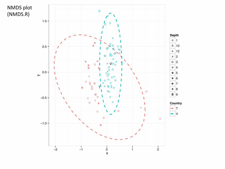
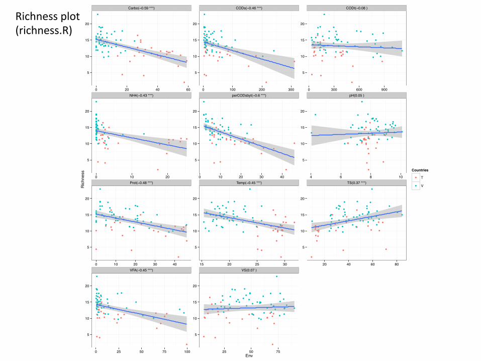
Carbo(−0.59 ***) CODs(−0.46 ***) CODt(−0.08 )
NH4(−0.43 ***) perCODsbyt(−0.6 ***) pH(0.05 )
Prot(−0.48 ***) Temp(−0.45 ***) TS(0.37 ***)
VFA(−0.45 ***) VS(0.07 )
5
10
15
20
5
10
15
20
5
10
15
20
5
10
15
20
5
10
15
20
5
10
15
20
5
10
15
20
5
10
15
20
5
10
15
20
5
10
15
20
5
10
15
20
0 20 40 60 0 100 200 300 0 300 600 900
0 10 20 0 10 20 30 40 4 6 8 10
0 10 20 30 40 15 20 25 30 20 40 60 80
0 25 50 75 100 25 50 75Env
Ric
hnes
s Countries
●
●
T
V
Richness plot (richness.R)
T_2_1T_2_10T_2_12T_2_2T_2_3T_2_6T_2_7T_2_9T_3_2T_3_3T_3_5T_4_3T_4_4T_4_5T_4_6T_4_7T_5_2T_5_3T_5_4T_5_5T_6_2T_6_5T_6_7T_6_8T_9_1T_9_2T_9_3T_9_4T_9_5V_1_2V_10_1V_11_1V_11_2V_11_3V_12_1V_12_2V_13_1V_13_2V_14_1V_14_2V_14_3V_15_1V_15_2V_15_3V_16_1V_16_2V_17_1V_17_2V_18_1V_18_2V_18_3V_18_4V_19_1V_19_2V_19_3V_2_1V_2_2V_2_3V_20_1V_21_1V_21_4V_22_1V_22_3V_22_4V_3_1V_3_2V_4_1V_4_2V_5_1V_5_3V_6_1V_6_2V_6_3V_7_1V_7_2V_7_3V_8_2V_9_1V_9_2V_9_3V_9_4
Acidobacteria_G
p1Acidobacteria_G
p10
Acidobacteria_G
p14
Acidobacteria_G
p16
Acidobacteria_G
p17
Acidobacteria_G
p18
Acidobacteria_G
p21
Acidobacteria_G
p22
Acidobacteria_G
p3Acidobacteria_G
p4Acidobacteria_G
p5Acidobacteria_G
p6Acidobacteria_G
p7Acidobacteria_G
p9Actinobacteria
Alphaproteobacteria
Anaerolineae
Bacilli
Bacteroidia
Betaproteobacteria
Caldilineae
Chlam
ydiae
Chloroflexi
Chrysiogenetes
Clostridia
Cyanobacteria
Dehalococcoidetes
Deinococci
Deltaproteobacteria
Epsilonproteobacteria
Erysipelotrichi
Fibrobacteria
Flavobacteria
Fusobacteria
Gam
maproteobacteria
Gem
matimonadetes
Holophagae
Lentisphaeria
Methanobacteria
Methanomicrobia
Mollicutes
Nitrospira
Opitutae
Planctom
ycetacia
Sphingobacteria
Spirochaetes
Subdivision3
Synergistia
Thermom
icrobia
Thermoplasm
ata
Thermotogae
Unknown
Species
Samples
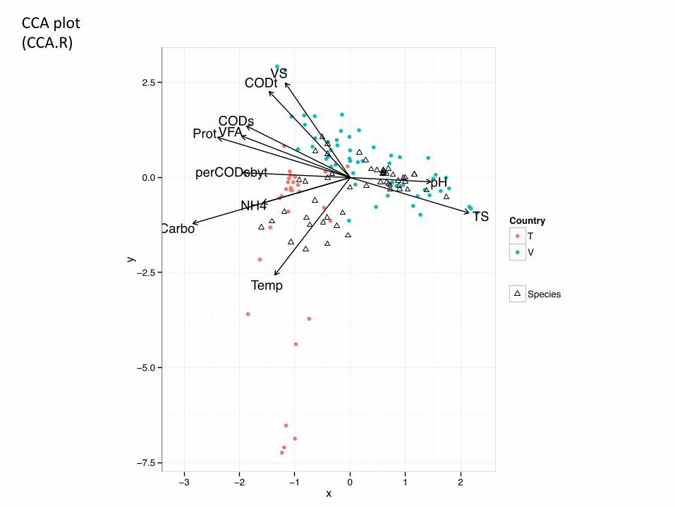
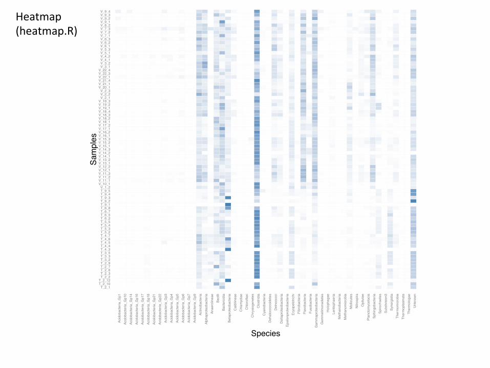
Heatmap (heatmap.R)
ggplot2 basics ggplot_basics.R
ggplot2
• Use just qplot(), without any understanding of the underlying grammar
• Theore/cal basis of ggplot2: layered grammar is based on Wilkinson’s grammar of graphics (Wilkinson, 2005)
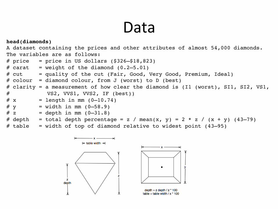
head(diamonds)!A dataset containing the prices and other attributes of almost 54,000 diamonds. !The variables are as follows:!# price = price in US dollars ($326–$18,823)!# carat = weight of the diamond (0.2–5.01)!# cut = quality of the cut (Fair, Good, Very Good, Premium, Ideal)!# colour = diamond colour, from J (worst) to D (best)!# clarity = a measurement of how clear the diamond is (I1 (worst), SI1, SI2, VS1, !# ! ! VS2, VVS1, VVS2, IF (best))!# x = length in mm (0–10.74)!# y = width in mm (0–58.9)!# z = depth in mm (0–31.8)!# depth = total depth percentage = z / mean(x, y) = 2 * z / (x + y) (43–79)!# table = width of top of diamond relative to widest point (43–95)!
Data
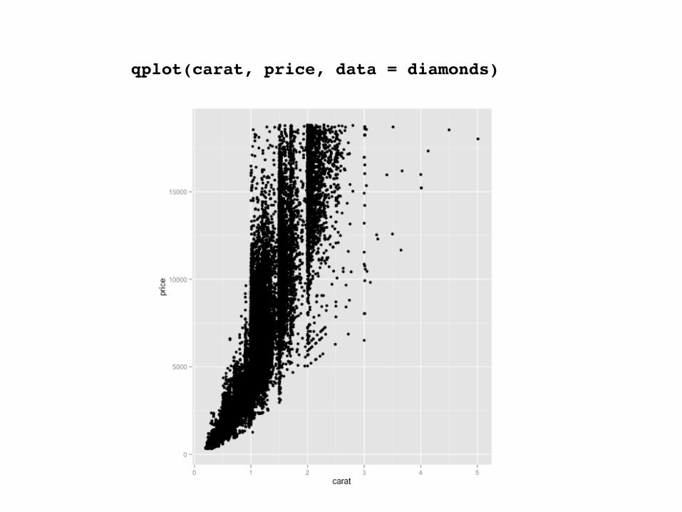
qplot(carat, price, data = diamonds)!
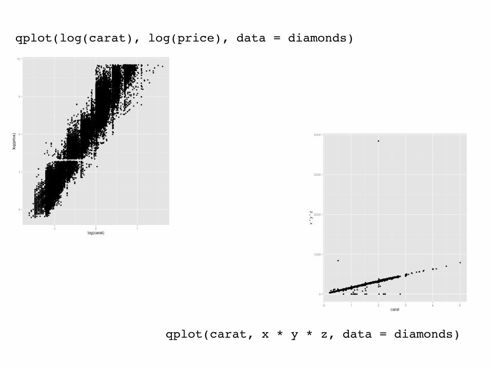
qplot(log(carat), log(price), data = diamonds)!
qplot(carat, x * y * z, data = diamonds)!
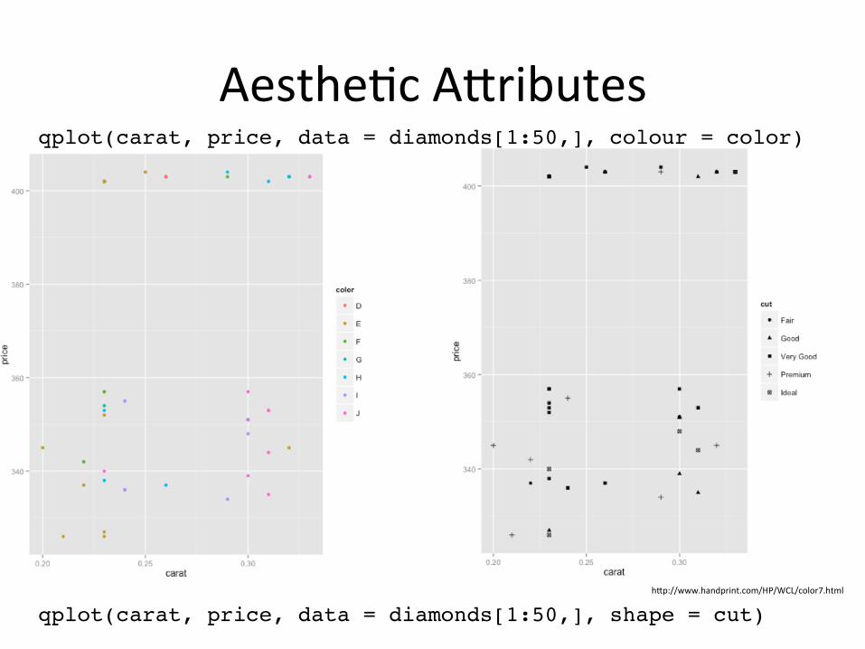
Aesthe/c A;ributes qplot(carat, price, data = diamonds[1:50,], colour = color)!
qplot(carat, price, data = diamonds[1:50,], shape = cut)!h;p://www.handprint.com/HP/WCL/color7.html
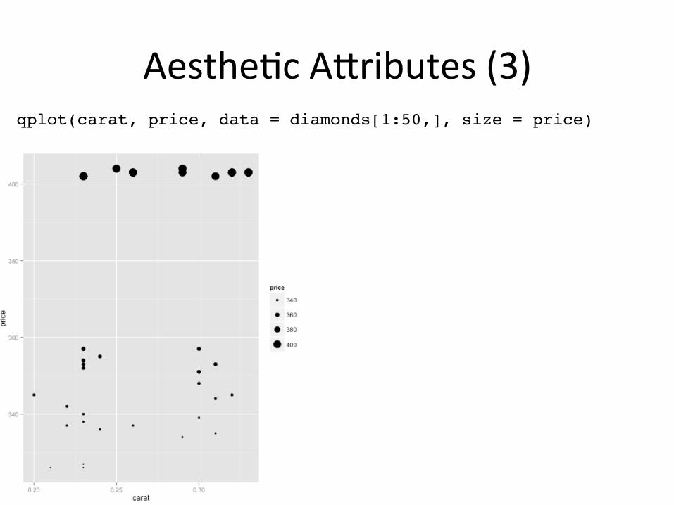
qplot(carat, price, data = diamonds[1:50,], size = price)!
Aesthe/c A;ributes (3)
Aesthe/c A;ributes (3)
• colour, size and shape are all examples of aesthe/c a;ributes, visual proper/es that affect the way observa/ons are displayed.
• For every aesthe/c a;ribute, there is a func/on, called a scale, which maps data values to valid values for that aesthe/c.
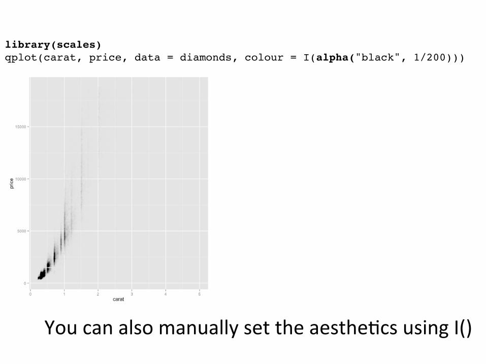
library(scales)!qplot(carat, price, data = diamonds, colour = I(alpha("black", 1/200)))!
You can also manually set the aesthe/cs using I()
Plot geoms(1) • geom = "point" draws points to produce a sca;erplot. This is the default when you supply both x and y arguments to qplot().
• geom = "smooth" fits a smoother to the data and displays the smooth and its standard error
• geom = "boxplot" produces a box and whisker plot to summarise the distribu/on of a set of points
• geom = "path" and geom = "line" draw lines between the data points.
• For con/nuous variables, geom = "histogram" draws a histogram, geom = "freqpoly" a frequency polygon, and geom = "density" creates a density plot
• For discrete variables, geom = "bar" makes a barchart
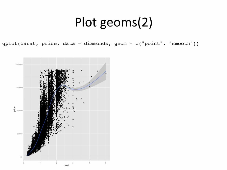
qplot(carat, price, data = diamonds, geom = c("point", "smooth"))!
Plot geoms(2)
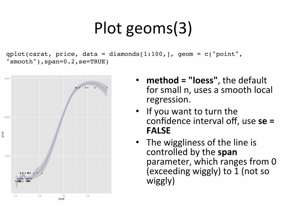
qplot(carat, price, data = diamonds[1:100,], geom = c("point", "smooth"),span=0.2,se=TRUE)!
Plot geoms(3)
• method = "loess", the default for small n, uses a smooth local regression.
• If you want to turn the confidence interval off, use se = FALSE
• The wiggliness of the line is controlled by the span parameter, which ranges from 0 (exceeding wiggly) to 1 (not so wiggly)
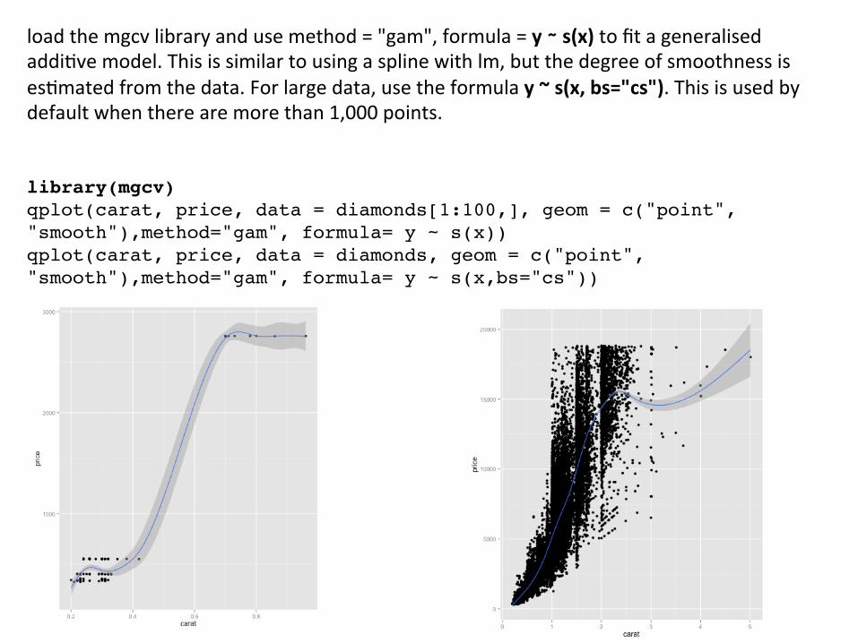
library(mgcv)!qplot(carat, price, data = diamonds[1:100,], geom = c("point", "smooth"),method="gam", formula= y ~ s(x))!qplot(carat, price, data = diamonds, geom = c("point", "smooth"),method="gam", formula= y ~ s(x,bs="cs"))!
load the mgcv library and use method = "gam", formula = y ∼ s(x) to fit a generalised addi/ve model. This is similar to using a spline with lm, but the degree of smoothness is es/mated from the data. For large data, use the formula y ~ s(x, bs="cs"). This is used by default when there are more than 1,000 points.
Plog geom(5)
library(splines)!qplot(carat, price, data = diamonds[1:100,], geom=c("point", "smooth"), method = "lm")!qplot(carat, price, data = diamonds[1:100,], geom=c("point", "smooth"), method = "lm", formula=y ~ poly(x,2))!qplot(carat, price, data = diamonds[1:100,], geom=c("point", "smooth"), method = "lm", formula=y ~ ns(x,3))!library(MASS)!qplot(carat, price, data = diamonds[1:100,], geom=c("point", "smooth"), method = "rlm")!
• method = "lm" fits a linear model. The default will fit a straight line to your data, or you can specify formula = y ~ poly(x, 2) to specify a degree 2 polynomial, or be;er, load the splines package and use a natural spline: formula = y ~ ns(x, 2). The second parameter is the degrees of freedom: a higher number will create a wigglier curve.
• method = "rlm" works like lm, but uses a robust fiang algorithm so that outliers don’t affect the fit as much
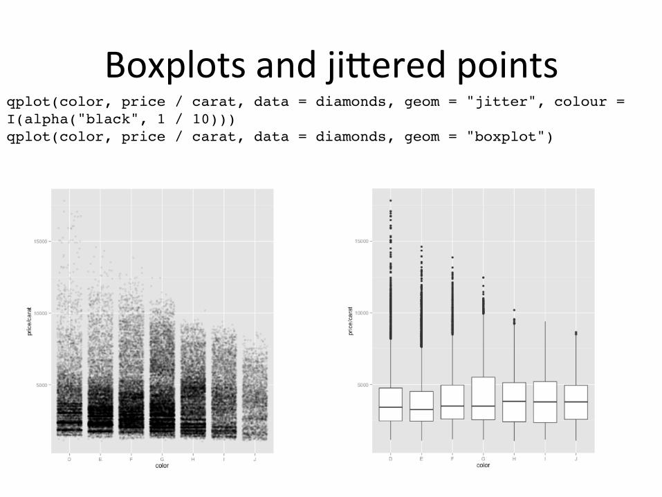
Boxplots and ji;ered points qplot(color, price / carat, data = diamonds, geom = "jitter", colour = I(alpha("black", 1 / 10)))!qplot(color, price / carat, data = diamonds, geom = "boxplot") !
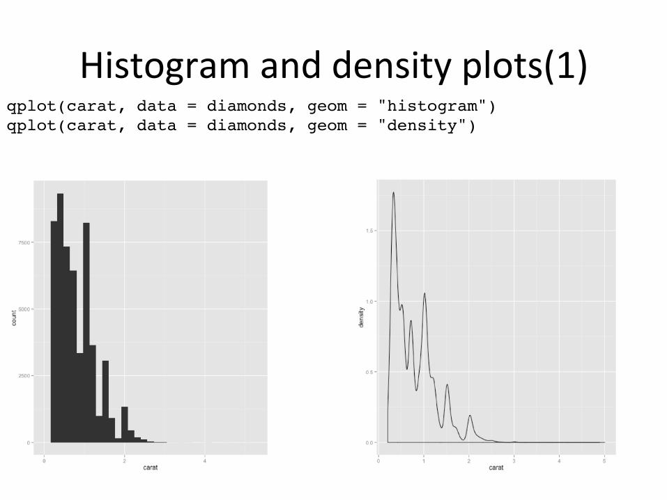
Histogram and density plots(1) qplot(carat, data = diamonds, geom = "histogram")!qplot(carat, data = diamonds, geom = "density")!

Histogram and density plots(2) qplot(carat, data = diamonds, geom = "histogram", fill = color)!qplot(carat, data = diamonds, geom = "density", colour = color)!
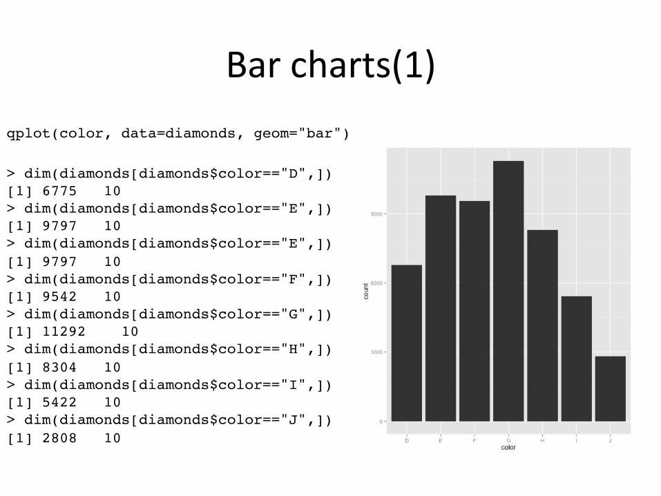
Bar charts(1)
> dim(diamonds[diamonds$color=="D",])![1] 6775 10!> dim(diamonds[diamonds$color=="E",])![1] 9797 10!> dim(diamonds[diamonds$color=="E",])![1] 9797 10!> dim(diamonds[diamonds$color=="F",])![1] 9542 10!> dim(diamonds[diamonds$color=="G",])![1] 11292 10!> dim(diamonds[diamonds$color=="H",])![1] 8304 10!> dim(diamonds[diamonds$color=="I",])![1] 5422 10!> dim(diamonds[diamonds$color=="J",])![1] 2808 10!
qplot(color, data=diamonds, geom="bar")!
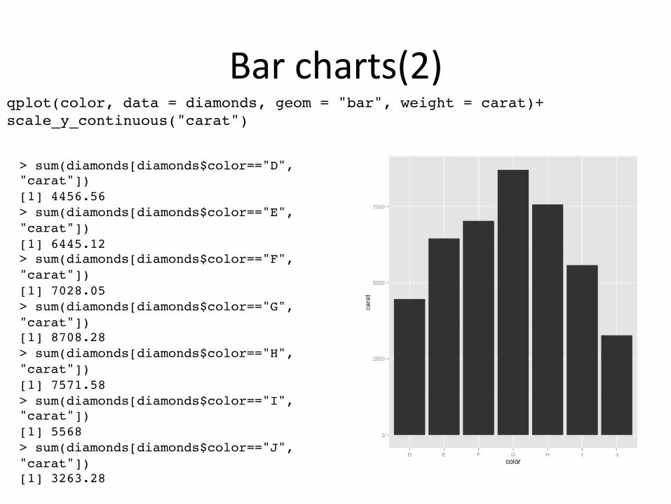
> sum(diamonds[diamonds$color=="D", "carat"])![1] 4456.56!> sum(diamonds[diamonds$color=="E", "carat"])![1] 6445.12!> sum(diamonds[diamonds$color=="F", "carat"])![1] 7028.05!> sum(diamonds[diamonds$color=="G", "carat"])![1] 8708.28!> sum(diamonds[diamonds$color=="H", "carat"])![1] 7571.58!> sum(diamonds[diamonds$color=="I", "carat"])![1] 5568!> sum(diamonds[diamonds$color=="J", "carat"])![1] 3263.28!
Bar charts(2) qplot(color, data = diamonds, geom = "bar", weight = carat)+ scale_y_continuous("carat")!
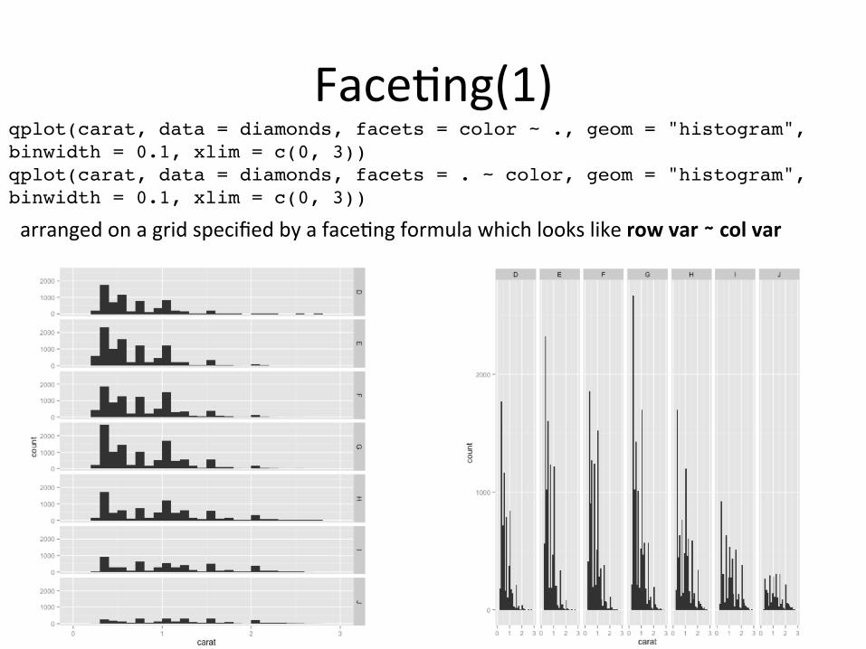
Face/ng(1) qplot(carat, data = diamonds, facets = color ~ ., geom = "histogram", binwidth = 0.1, xlim = c(0, 3))!qplot(carat, data = diamonds, facets = . ~ color, geom = "histogram", binwidth = 0.1, xlim = c(0, 3))!
arranged on a grid specified by a face/ng formula which looks like row var ∼ col var
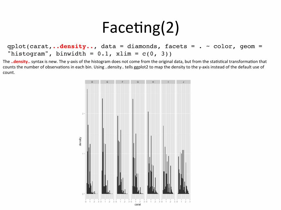
qplot(carat,..density.., data = diamonds, facets = . ~ color, geom = "histogram", binwidth = 0.1, xlim = c(0, 3))!
Face/ng(2)
The ..density.. syntax is new. The y-‐axis of the histogram does not come from the original data, but from the sta/s/cal transforma/on that counts the number of observa/ons in each bin. Using ..density.. tells ggplot2 to map the density to the y-‐axis instead of the default use of count.
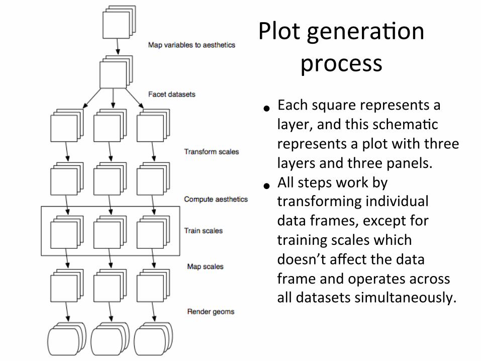
Plot genera/on process
• Each square represents a layer, and this schema/c represents a plot with three layers and three panels.
• All steps work by transforming individual data frames, except for training scales which doesn’t affect the data frame and operates across all datasets simultaneously.
Layers
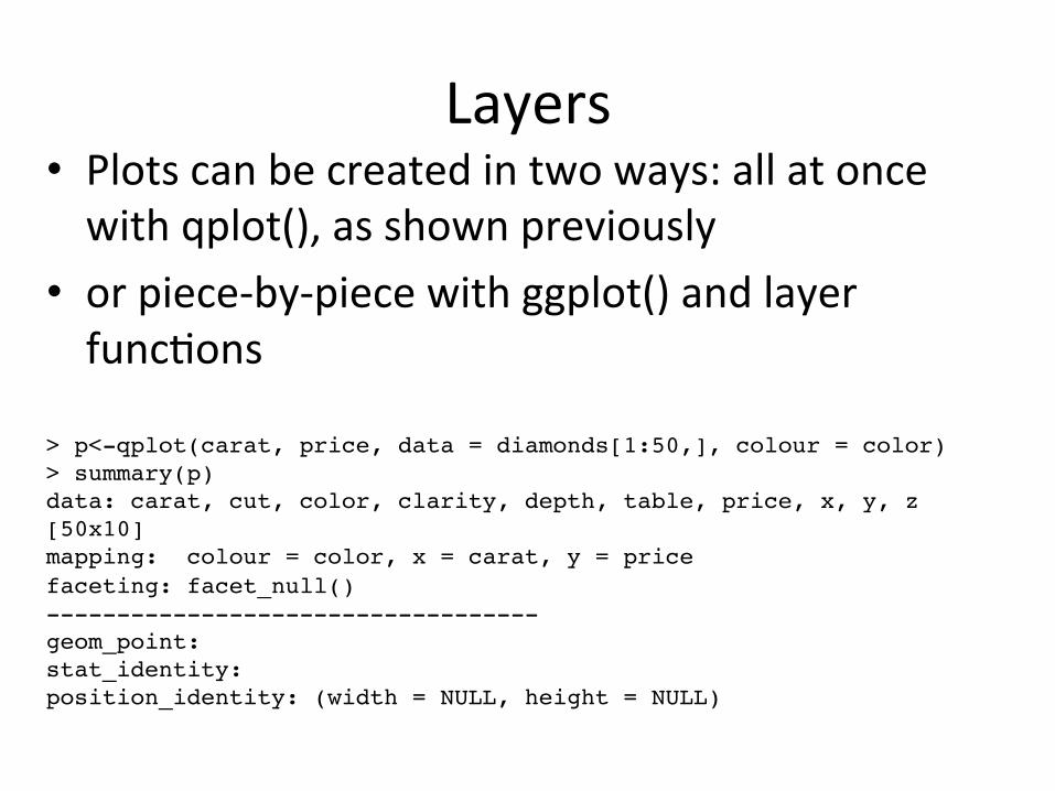
> p<-qplot(carat, price, data = diamonds[1:50,], colour = color)!> summary(p)!data: carat, cut, color, clarity, depth, table, price, x, y, z [50x10]!mapping: colour = color, x = carat, y = price!faceting: facet_null() !-----------------------------------!geom_point: !stat_identity: !position_identity: (width = NULL, height = NULL)!
• Plots can be created in two ways: all at once with qplot(), as shown previously
• or piece-‐by-‐piece with ggplot() and layer func/ons
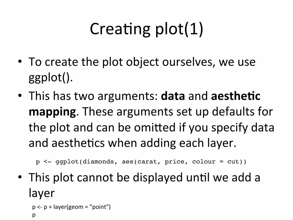
Crea/ng plot(1)
• To create the plot object ourselves, we use ggplot().
• This has two arguments: data and aestheGc mapping. These arguments set up defaults for the plot and can be omi;ed if you specify data and aesthe/cs when adding each layer.
• This plot cannot be displayed un/l we add a layer
p <- ggplot(diamonds, aes(carat, price, colour = cut))!
p <-‐ p + layer(geom = "point") p
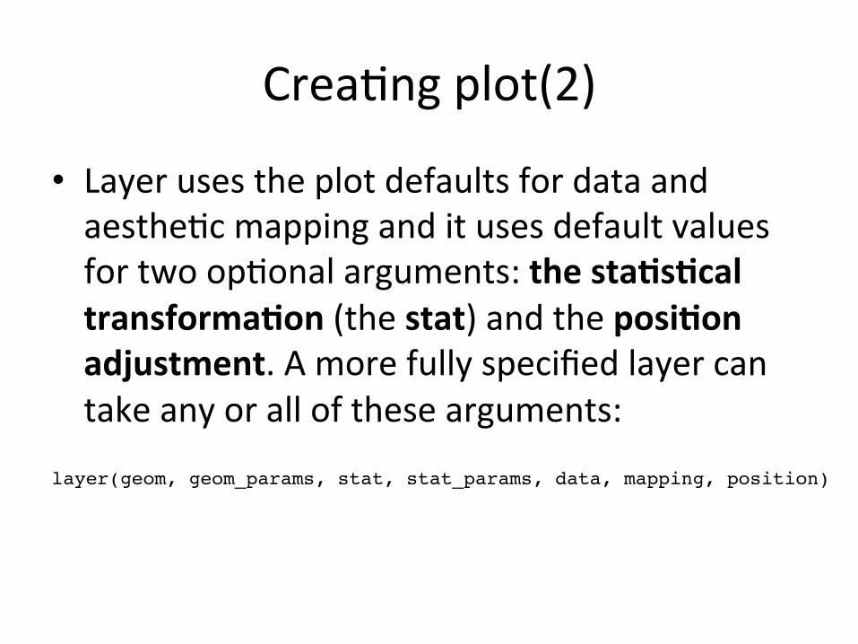
Crea/ng plot(2)
• Layer uses the plot defaults for data and aesthe/c mapping and it uses default values for two op/onal arguments: the staGsGcal transformaGon (the stat) and the posiGon adjustment. A more fully specified layer can take any or all of these arguments:
layer(geom, geom_params, stat, stat_params, data, mapping, position)!
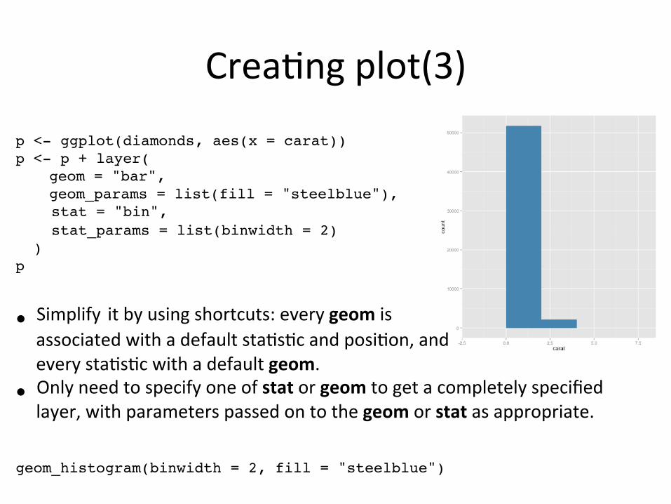
Crea/ng plot(3)
p <- ggplot(diamonds, aes(x = carat))!p <- p + layer(!
!geom = "bar",!!geom_params = list(fill = "steelblue"),!
stat = "bin",! stat_params = list(binwidth = 2)! ) !p!
• Simplify it by using shortcuts: every geom is associated with a default sta/s/c and posi/on, and every sta/s/c with a default geom.
• Only need to specify one of stat or geom to get a completely specified layer, with parameters passed on to the geom or stat as appropriate.
geom_histogram(binwidth = 2, fill = "steelblue")!
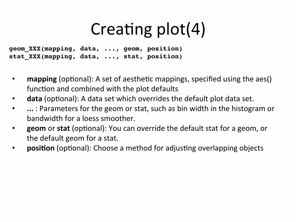
Crea/ng plot(4) !geom_XXX(mapping, data, ..., geom, position)!stat_XXX(mapping, data, ..., stat, position)!
• mapping (op/onal): A set of aesthe/c mappings, specified using the aes() func/on and combined with the plot defaults
• data (op/onal): A data set which overrides the default plot data set. • ... : Parameters for the geom or stat, such as bin width in the histogram or
bandwidth for a loess smoother. • geom or stat (op/onal): You can override the default stat for a geom, or
the default geom for a stat. • posiGon (op/onal): Choose a method for adjus/ng overlapping objects
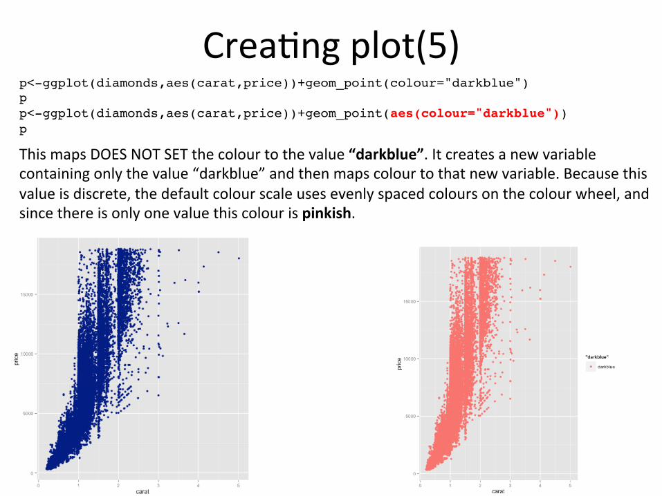
Crea/ng plot(5) p<-ggplot(diamonds,aes(carat,price))+geom_point(colour="darkblue")!p!p<-ggplot(diamonds,aes(carat,price))+geom_point(aes(colour="darkblue"))!p!
This maps DOES NOT SET the colour to the value “darkblue”. It creates a new variable containing only the value “darkblue” and then maps colour to that new variable. Because this value is discrete, the default colour scale uses evenly spaced colours on the colour wheel, and since there is only one value this colour is pinkish.
• geoms can be individual and collec/ve geoms • By default, group is set to the interac/on of all discrete variables in the plot
• When it doesn’t, explicitly define the grouping structure, by mapping group to a variable that has a different value for each group
• interacGon() is useful if a single pre-‐exis/ng variable doesn’t cleanly separate groups
Crea/ng plot(6): Grouping
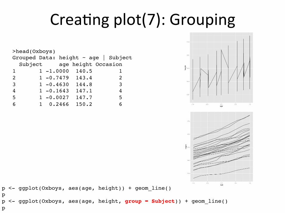
>head(Oxboys)!Grouped Data: height ~ age | Subject! Subject age height Occasion!1 1 -1.0000 140.5 1!2 1 -0.7479 143.4 2!3 1 -0.4630 144.8 3!4 1 -0.1643 147.1 4!5 1 -0.0027 147.7 5!6 1 0.2466 150.2 6!
p <- ggplot(Oxboys, aes(age, height)) + geom_line()!p!p <- ggplot(Oxboys, aes(age, height, group = Subject)) + geom_line()!p!
Crea/ng plot(7): Grouping
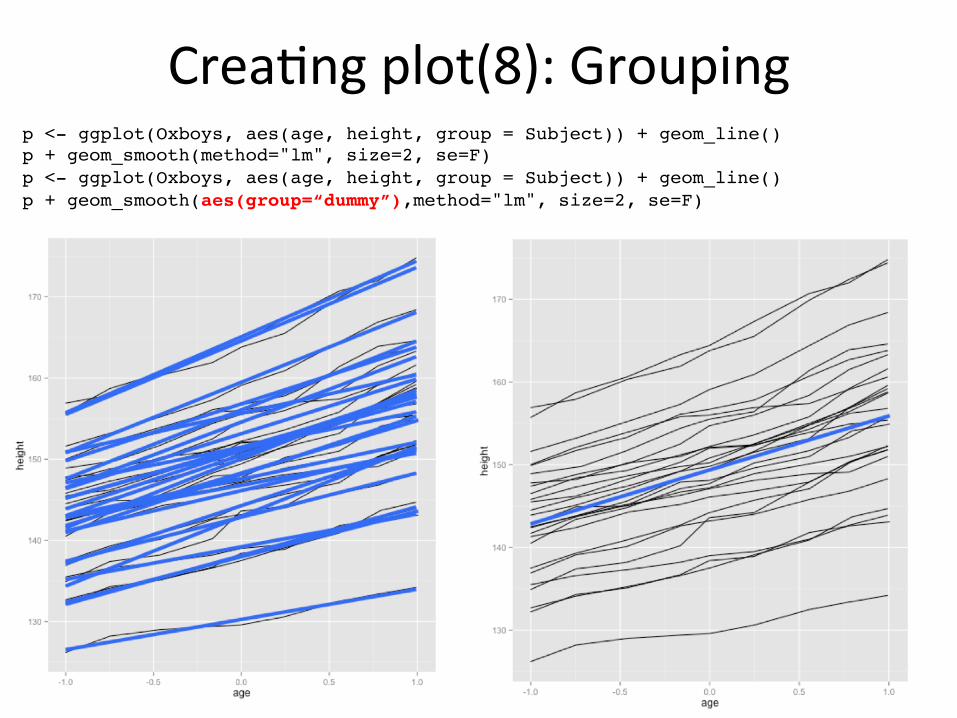
p <- ggplot(Oxboys, aes(age, height, group = Subject)) + geom_line()!p + geom_smooth(method="lm", size=2, se=F)!p <- ggplot(Oxboys, aes(age, height, group = Subject)) + geom_line()!p + geom_smooth(aes(group=“dummy”),method="lm", size=2, se=F)!
Crea/ng plot(8): Grouping
Geoms
• Geometric objects (geoms) – Perform the actual rendering of the layer – Control the type of plot that you create – Has a set of aesthe/cs – Differ in the way they are parameterised – Have a default sta/s/c
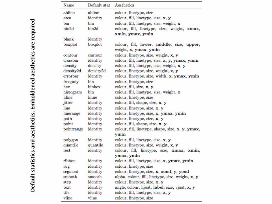
Default staGsGcs a
nd aestheG
cs. Embo
lden
ed aestheG
cs are re
quire
d
Stat(1) • Sta/s/cal transforma/on (stat)
– Transforms the data by summarising it in some manner – e.g., smoother calculates the mean of y, condi/on of x – A stat must be loca/on-‐scale invariant (transforma/on stays same when scale is changed) f(x+a)=f(x)+a ; f(b.x)=b.f(x)
– Takes a dataset as input, returns a dataset as output and introduces new variables
– e.g., stat_bin (sta/s/c used to make histograms, produces) • count: number of observa/on in each bin • density: density of observa/on in each bin (percentage of total/bar width)
• x: the centre of bin – The names of generated variables must be surrounded with .. when used
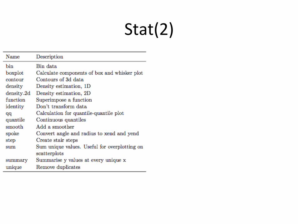
Stat(2)
Posi/on adjustments(1)
• Apply minor tweaks to the posi/on of elements within a layer
• Normally used with discrete data • Con/nuous data typically don’t overlap and when do, jiOering is sufficient
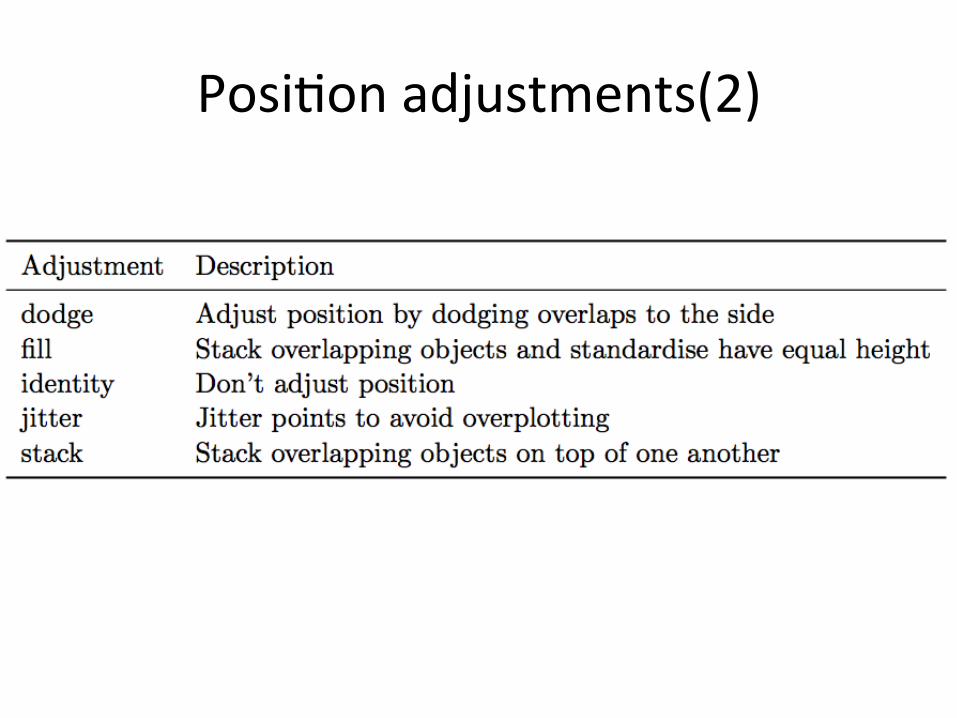
Posi/on adjustments(2)
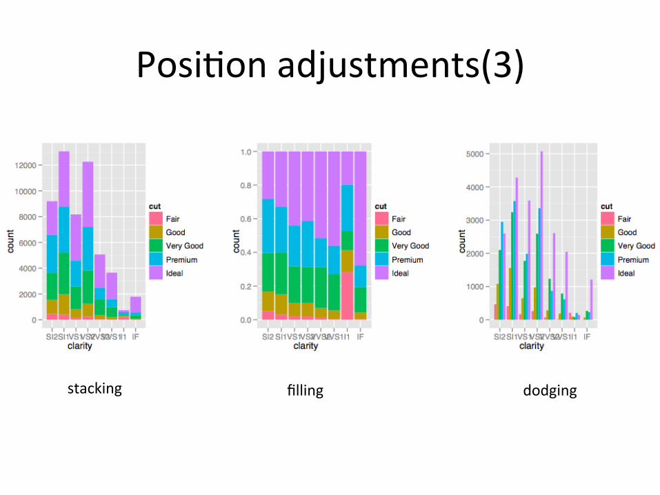
Posi/on adjustments(3)
stacking filling dodging
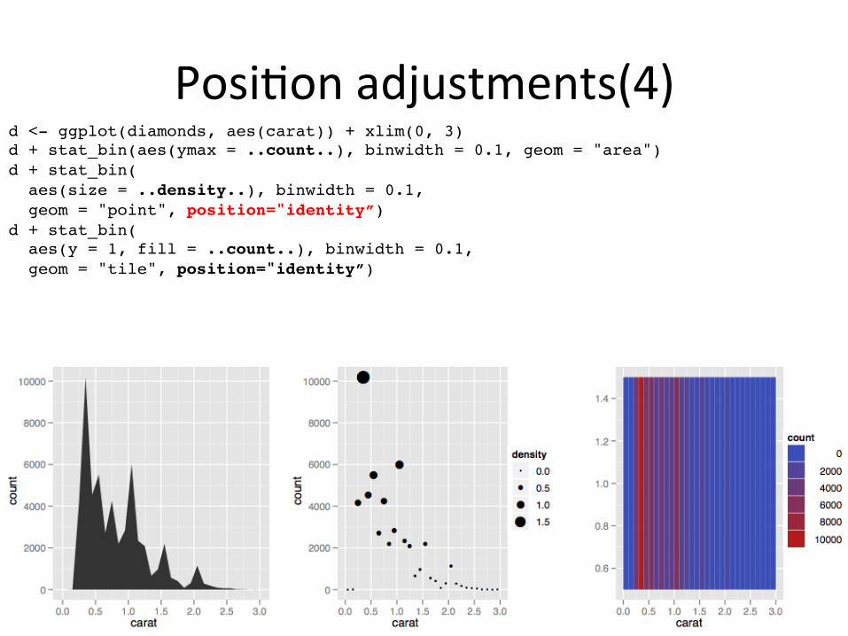
Posi/on adjustments(4) d <- ggplot(diamonds, aes(carat)) + xlim(0, 3)!d + stat_bin(aes(ymax = ..count..), binwidth = 0.1, geom = "area")!d + stat_bin(! aes(size = ..density..), binwidth = 0.1,! geom = "point", position="identity”)!d + stat_bin(! aes(y = 1, fill = ..count..), binwidth = 0.1,! geom = "tile", position="identity”)!
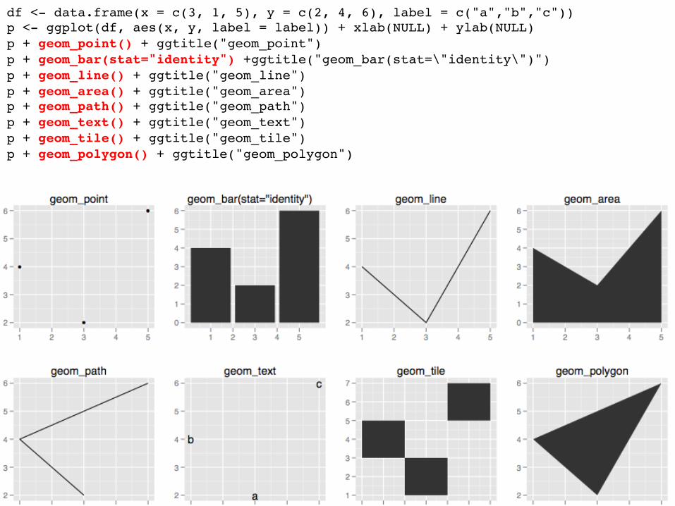
df <- data.frame(x = c(3, 1, 5), y = c(2, 4, 6), label = c("a","b","c"))!p <- ggplot(df, aes(x, y, label = label)) + xlab(NULL) + ylab(NULL)!p + geom_point() + ggtitle("geom_point")!p + geom_bar(stat="identity") +ggtitle("geom_bar(stat=\"identity\")")!p + geom_line() + ggtitle("geom_line")!p + geom_area() + ggtitle("geom_area")!p + geom_path() + ggtitle("geom_path")!p + geom_text() + ggtitle("geom_text")!p + geom_tile() + ggtitle("geom_tile")!p + geom_polygon() + ggtitle("geom_polygon")!
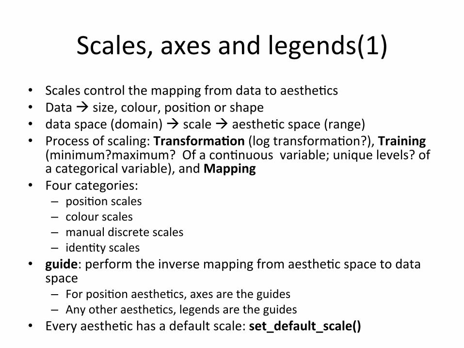
Scales, axes and legends(1) • Scales control the mapping from data to aesthe/cs • Data à size, colour, posi/on or shape • data space (domain) à scale à aesthe/c space (range) • Process of scaling: TransformaGon (log transforma/on?), Training
(minimum?maximum? Of a con/nuous variable; unique levels? of a categorical variable), and Mapping
• Four categories: – posi/on scales – colour scales – manual discrete scales – iden/ty scales
• guide: perform the inverse mapping from aesthe/c space to data space – For posi/on aesthe/cs, axes are the guides – Any other aesthe/cs, legends are the guides
• Every aesthe/c has a default scale: set_default_scale()
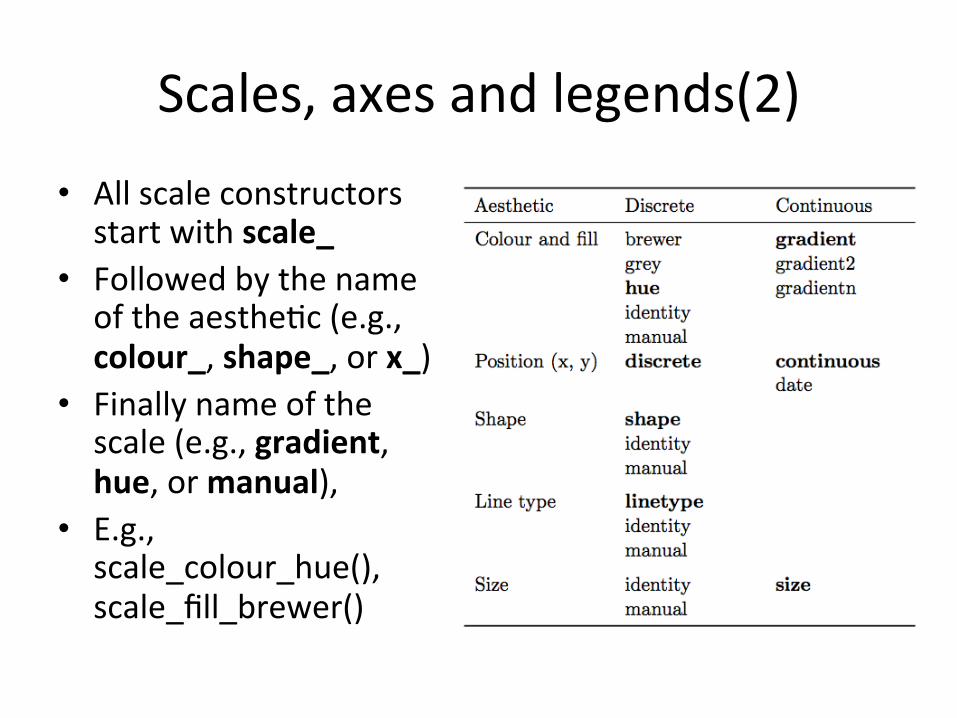
Scales, axes and legends(2)
• All scale constructors start with scale_
• Followed by the name of the aesthe/c (e.g., colour_, shape_, or x_)
• Finally name of the scale (e.g., gradient, hue, or manual),
• E.g., scale_colour_hue(), scale_fill_brewer()
Scale example
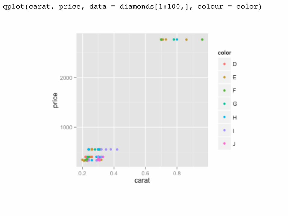
qplot(carat, price, data = diamonds[1:100,], colour = color) !
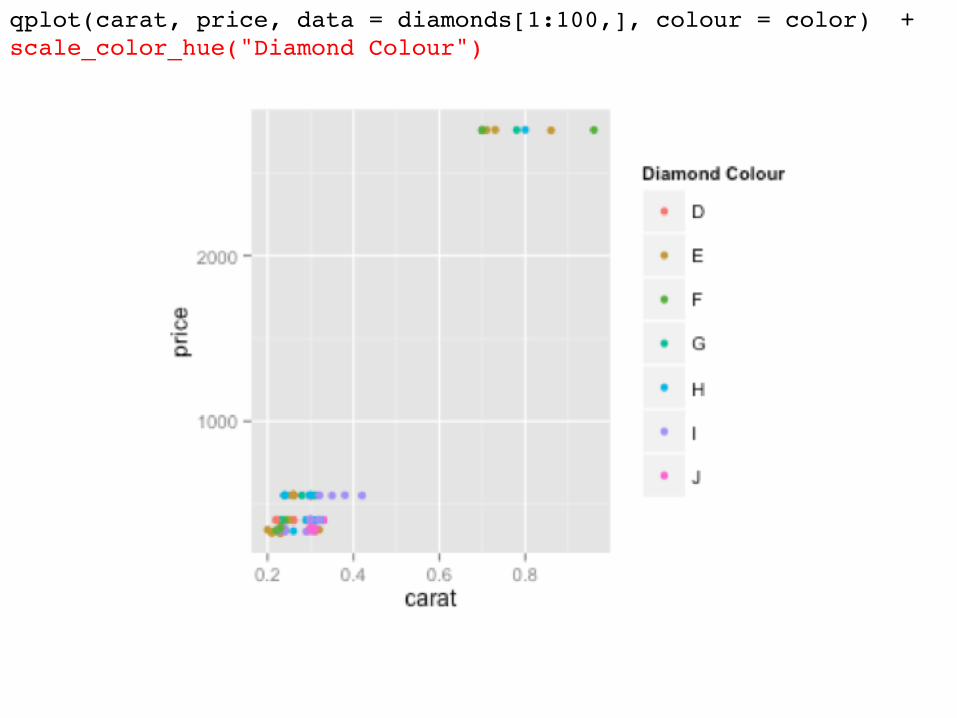
qplot(carat, price, data = diamonds[1:100,], colour = color) + scale_color_hue("Diamond Colour")!
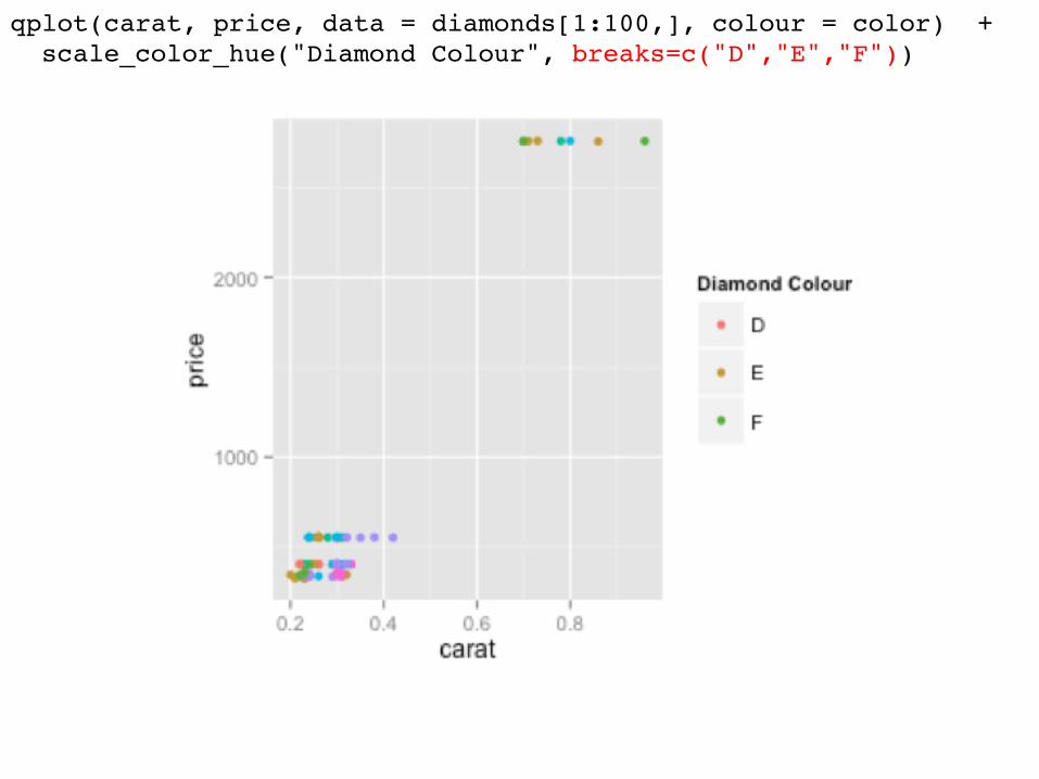
qplot(carat, price, data = diamonds[1:100,], colour = color) + ! scale_color_hue("Diamond Colour", breaks=c("D","E","F"))!
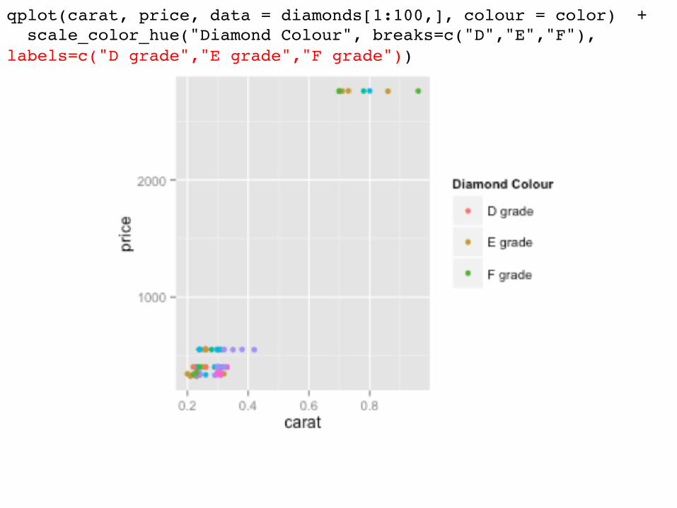
qplot(carat, price, data = diamonds[1:100,], colour = color) + ! scale_color_hue("Diamond Colour", breaks=c("D","E","F"), labels=c("D grade","E grade","F grade"))!
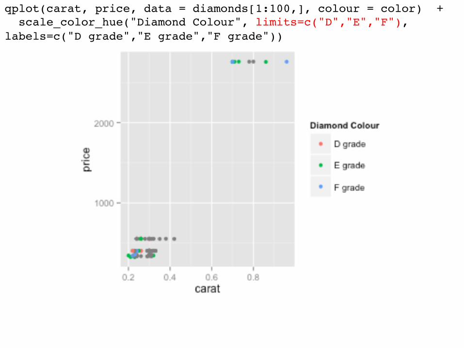
qplot(carat, price, data = diamonds[1:100,], colour = color) + ! scale_color_hue("Diamond Colour", limits=c("D","E","F"), labels=c("D grade","E grade","F grade"))!
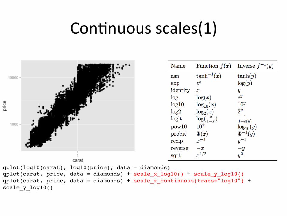
Con/nuous scales(1)
qplot(log10(carat), log10(price), data = diamonds)!qplot(carat, price, data = diamonds) + scale_x_log10() + scale_y_log10()!qplot(carat, price, data = diamonds) + scale_x_continuous(trans="log10") + scale_y_log10()!
Con/nuous scales(2)
• scale_colour_gradient() and scale_fill_gradient(): a two–colour gradient, low–high. Arguments low and high control the colours at either end of the gradient.
• scale_colour_gradient2() and scale_fill_gradient2(): a three–colour gradient, low–med–high.
• scale_colour_gradientn() and scale_fill_gradientn(): a custom n–colour gra-‐ dient.
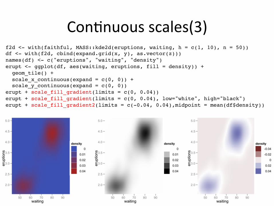
f2d <- with(faithful, MASS::kde2d(eruptions, waiting, h = c(1, 10), n = 50))!df <- with(f2d, cbind(expand.grid(x, y), as.vector(z)))!names(df) <- c("eruptions", "waiting", "density")!erupt <- ggplot(df, aes(waiting, eruptions, fill = density)) +! geom_tile() +! scale_x_continuous(expand = c(0, 0)) +! scale_y_continuous(expand = c(0, 0))!erupt + scale_fill_gradient(limits = c(0, 0.04))!erupt + scale_fill_gradient(limits = c(0, 0.04), low="white", high="black")!erupt + scale_fill_gradient2(limits = c(-0.04, 0.04),midpoint = mean(df$density))!
Con/nuous scales(3)
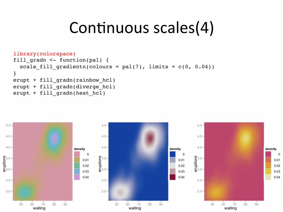
Con/nuous scales(4) library(colorspace)!fill_gradn <- function(pal) {! scale_fill_gradientn(colours = pal(7), limits = c(0, 0.04))!}!erupt + fill_gradn(rainbow_hcl)!erupt + fill_gradn(diverge_hcl)!erupt + fill_gradn(heat_hcl)!