Embed Size (px)
DESCRIPTION
hhhhh
Citation preview
SIMULATION OF BOILER DYNAMICS— Development, Evaluation and Applicationof a General Energy System Simulation Tool
Brian Elmegaard
Ph.D. Thesis
ET–PhD 99–02
1999
Technical University of Denmark
Brian Elmegaard
SIMULATION OF BOILER DYNAMICS– Development, Evaluation and Application of a General EnergySystem Simulation Tool
Technical University of Denmark, Department of Energy EngineeringPh.D. Thesis: Report Number ET–PhD 99–02
Printed by Tekst & Tryk A/S, Vedbæk, DenmarkISBN 87–7475–222–7
Copyright c©1999 by Brian Elmegaard


ACKNOWLEDGEMENTS
This thesis concludes a three year Ph.D. study at the Energy Systems groupof the Department of Energy Engineering, Technical University of Denmark.The subjects covered in this thesis, however, is only part of the many differentaspects of research and engineering, I have had the possibility to encounterduring the study.
The work has been supervised by Associate Professor Niels Houbak, whohas willingly supported me with encouraging spirit when wanted, and hassupplied me with the necessary insight whenever needed.
My fellow Ph.D. students at the Department also should receive my grat-itude. It has been a pleasure work with you. M.Sc., Ph.D. Jens BjerremandMikkelsen whose office I sieged and gradually won with help from my army ofwork stations, and M.Sc. Anne Rasmussen are acknowledged. M.Sc. HenrikDalsgard and M.Sc. Falko Jens Wagner are hereby wished the best for theirprojects. All students supplying me with good proposals for improvementsof DNA and pointing out the pieces of the code which needed a fix are alsoacknowledged.
The three years have taken me far about both geographically and profes-sionally. I must give all my thanks to the staff of the Section Thermal PowerEngineering of the Delft University of Technology. Especially, M.Sc. ArieKorving who made my stay in Delft possible and who did whatever he couldto make this stay pleasant, is gratefully thanked for his kind reply to myrequest, and for the nice times we have had together since the first day wemet in Delft.
Last, my wife, Karen, who throughout my study has been supplying mewith clever advice, psychological assistance and project management shouldreceive my deepest gratitude. Also, my wife and our children need to bethanked for willingly moving our home with me to the Netherlands for atemporary stay and for always being able to make any trouble with my workfade away for a while and thereby allowing new ideas to develop in a pleasantatmosphere.
Birkerød, August 1999Brian Elmegaard

ii
ABSTRACT
This thesis describes the work done in order to make the simulator DNAapplicable in simulation of dynamics of a modern natural gas fired boiler.The study aims at modelling and simulating the boiler of Skærbækværketunit 3, which has been used for exemplification. The boiler is operated withsliding pressure at a maximum of 350 bar.
DNA is a flexible program for literally any energy system. The programhas features for simulation of the mathematical models, which are the res-ults of modelling studies of thermodynamic processes. The program handlesmodels of both steady state and transient processes. By use of a modellingprocedure equivalent to network theory used in electrical engineering, an ex-pedient modelling methodology for thermodynamic processes is applied. Acomponent library featuring a number of component models is available inDNA. This has been maintained and further developed.
DNA is the result of several previous development studies. The programhas been developed with a six-point framework in mind. The framework istermed PREFUR, which is an acronym for Portability between operating sys-tems, Robustness, Efficiency, Flexibility, User Friendliness and Readabilityof the source code. This framework has also been the basis for the exten-sions of DNA made throughout this work. To take advantage of previousworks, the present work mainly has focussed on the development of betteruser friendliness, robustness and flexibility of the program and the compon-ent models. An assessment of improvement of efficiency and performance ofthe numerical solver of DNA is also featured.
The main improvements of the code are: Handling of discontinuous equa-tions in dynamic systems, generalization and increase of robustness of com-ponent models, implementation of relations for transport properties and ra-diative properties of fluids relevant in power engineering, and implementationof thermodynamic properties of solid fuels and ashes.
Many simulators for different kinds of power plants are available. A num-ber of these have been investigated by application and through a literaturesurvey. Particularly the program Cycle-Tempo has been used and comparedto DNA. An evaluation of DNA based on the survey shows, that DNA pos-
iv
sesses features which a hardly available in other programs of its kind, butalso that other programs have better facilities for some tasks.
The component library has been extended to be able to carry out thesimulations needed for the two application studies made. One is the study ofboiler dynamics. The other is a design and optimization study of a biomass-based IGCC plant. Some of the already present components have been ex-tended to be robust and general. Two of these are an extraction turbine andheat exchanger models. Heat exchangers models are difficult to work with,due to problems with violation of the Second Law of Thermodynamics duringnumerical solving of a model. The developed model is highly robust. For theboiler model steady-state and dynamic models for furnace and superheatershave been developed. For the BIGCC system a set of relevant componentsfor solid fuels have been included in the library.
The study of the boiler of Skærbækværket unit 3 shows that DNA isapplicable in studies of complex, dynamic energy systems. A model of theboiler, including furnace, downcomer, separator, superheaters and reheatershas been developed and has been set up based on full load data. Results ofa simulation of a load change from 39% to 33% of the boiler with the modelhas been verified by comparison to data.
The purposes of the BIGCC study have been to compare the results ofDNA and Cycle-Tempo, when applied in simulation of a complex energysystem, and to suggest improvements of the better process of those found tobe available during a literature survey.
RESUME
Nærværende rapport beskriver det arbejde, som er udført for at gøre simule-ringsprogrammet DNA anvendeligt i forbindelse med simulering af dynamiskeforhold for en moderne, naturgasfyret kraftværkskedel. Studiet har haft somoverordnet mal, at modellere og simulere kedlen pa Skærbækværkets blok 3,som er anvendt for eksemplificering. Kedlen er udlagt for glidetryksdrift medet maksimalt tryk pa 350 bar.
DNA er et fleksibelt program, som kan anvendes for praktisk talt et-hvert energisystem. Programmet har faciliteter for simulering af de mate-matiske modeller, der er resultat af modelleringsstudier for termodynamiskeprocesser. Programmet handterer bade modeller af stationære og transienteprocesser. Ved at benytte en modelleringsteknik, baseret pa netværksteorianvendt pa elektriske kredsløb, opnas en hensigtsmæssig formulering af mo-deller for termodynamiske processer. DNA inkluderer et komponentbibliotekmed modeller for et antal komponenter, der er relevante for energisystemer.Komponentbiblioteket er blevet opdateret i henhold til udvikling af DNA ognye modeller er implementeret.
DNA er resultatet af flere tidligere studier. Programmet er undervejs ble-vet udviklet i henhold til et seks-punkts-koncept. Dette koncept er betegnetPREFUR, som er et (engelsk) akronym for Portabilitet mellem operativsy-stemer, Robusthed, Effektivitet, Fleksibilitet, Brugervenlighed og Læsbarhedaf kildeteksten. Konceptet har ligeledes været rammen for de udvidelser afDNA, der er foretaget under projektet. En gennemgang af de tidligere arbej-der med programmet har vist, at der fortrinsvis har været behov for udviklingaf bedre brugervenlighed, robusthed og fleksibilitet af programmet i sig selvog af komponentmodeller. Desuden er forbedringer af effektiviteten af dennumeriske løser i DNA blevet implementeret.
De vigtigste forbedringer af koden er: Handtering af diskontinuerte lig-ninger i dynamiske systemer, generalisering og forbedring af robusthed afkomponentmodeller, implementering af relationer for transportvariable ogstralingsegenskaber for fluider, der er relevante i kraftværkssammenhæng ogimplementering af termodynamiske egenskaber for faste brændsler og aske.
En del simuleringsprogrammer for forskellige typer af kraftværksanlæg er
vi
tilgængelige. Et antal af disse er blevet undersøgt via anvendelse og littera-turstudie. Specielt er programmet Cycle-Tempo blevet anvendt og sammen-lignet med DNA. En evaluering af DNA baseret pa denne undersøgelse viser,at andre programmer med samme faciliteter som DNAs næppe findes. Un-dersøgelsen viser dog ogsa, at andre programmer pa nogle punkter er DNAoverlegent.
Komponentbiblioteket er blevet udvidet for at kunne udføre de simule-ringer, der har været nødvendige i to case-studier vedrørende anvendelse afDNA. Det ene er studiet af dynamiske forhold for kedler. Det andet er etdesign- og optimeringsstudie af et biomassebaseret IGCC-anlæg. Nogle af deallerede eksisterende komponentmodeller er blevet udvidet med henblik paat gøre dem robuste og generelle. To af disse er en turbine med dampudtagog varmevekslermodeller. Varmevekslermodeller er besværlige at anvende, datermodynamikkens anden hovedsætning kan blive overtradt under den nu-meriske løsning af en model. Den nyudviklede model er robust overfor dette.For kedelmodellen er bade steady-state og dynamiske modeller for fyrrum ogoverhedere blevet udviklet. I forbindelse med BIGCC-anlægget er et antal re-levante kompontmodeller for anvendelse af faste brændsler blevet inkludereti biblioteket.
Studiet af kedlen pa Skærbækværkets blok 3 viser, at DNA kan benyttesved studier af komplekse, dynamiske energisystemer. En model af kedlen, sominkluderer fyrrum, faldrør, dampseparering, overhedere og genoverhedere erblevet udviklet og er implementeret baseret pa designlast-data for værket.Resultater af simulering af denne model for en lastændring fra 39% til 33%for kedlen er blevet verificeret ved sammenligning med driftsdata.
Formalene med studiet af BIGCC-anlægget har været at sammenligneresultater fra DNA og Cycle-Tempo ved anvendelse til simulering af et kom-plekst energisystem, og at foresla mulige procesforbedringer for den bedsteaf de anlægskonfigurationer, som er fundet ved et litteraturstudie.
CONTENTS
1. Introduction . . . . . . . . . . . . . . . . . . . . . . . . . . . . . . 11.1 Modelling and Simulation of Energy Systems . . . . . . . . . . 11.2 The Modelling Process . . . . . . . . . . . . . . . . . . . . . . 11.3 DNA . . . . . . . . . . . . . . . . . . . . . . . . . . . . . . . . 3
1.3.1 PREFUR – A Framework for Code Development . . . 31.3.2 History of DNA . . . . . . . . . . . . . . . . . . . . . . 4
1.4 Simulation of Boiler Dynamics . . . . . . . . . . . . . . . . . . 51.5 Simulation of a Biomass-based Integrated Gasification/Com-
bined Cycle Plant . . . . . . . . . . . . . . . . . . . . . . . . . 61.6 Objective of the Study . . . . . . . . . . . . . . . . . . . . . . 6
2. Basis for the Study of Boiler Dynamics . . . . . . . . . . . . . . 92.1 Technological Status in Boiler Simulation . . . . . . . . . . . . 9
2.1.1 Description of Boiler Dynamics . . . . . . . . . . . . . 92.1.2 Modelling Dynamic Processes of Power Plant Boilers . 10
2.2 Physical phenomena . . . . . . . . . . . . . . . . . . . . . . . 122.2.1 Fundamental Characteristics of the Boiler Model . . . 122.2.2 Combustion Modelling . . . . . . . . . . . . . . . . . . 142.2.3 Furnace Model . . . . . . . . . . . . . . . . . . . . . . 142.2.4 Superheater Section Model . . . . . . . . . . . . . . . . 182.2.5 Relevant Dynamic Features of Boiler Design . . . . . . 19
3. Development of the DNA Code . . . . . . . . . . . . . . . . . . . 213.1 Underlying Theory of DNA . . . . . . . . . . . . . . . . . . . 213.2 DNA Models . . . . . . . . . . . . . . . . . . . . . . . . . . . 24
3.2.1 Algebraic Loops . . . . . . . . . . . . . . . . . . . . . . 263.3 Mathematical Model . . . . . . . . . . . . . . . . . . . . . . . 28
3.3.1 Formulation of Lumped Parameter Component Models 283.3.2 Resulting System of Equations . . . . . . . . . . . . . . 30
3.4 Numerical Methods in Simulators . . . . . . . . . . . . . . . . 303.4.1 Methodology for Solution of Equation Systems . . . . . 323.4.2 Methodology for Solution of Differential Equations . . 33
viii Contents
3.5 Numerical Methods of DNA . . . . . . . . . . . . . . . . . . . 333.6 The Modified Newton Method . . . . . . . . . . . . . . . . . . 34
3.6.1 Evaluation of the Jacobian Matrix . . . . . . . . . . . 353.6.2 Controlling the Update of the Jacobian Matrix . . . . . 373.6.3 Initialization of the Method . . . . . . . . . . . . . . . 373.6.4 The Problem of Ensuring Convergence and that Solu-
tions are Correct . . . . . . . . . . . . . . . . . . . . . 383.6.5 Generation of Initial Guesses . . . . . . . . . . . . . . . 413.6.6 Generalization of Component Models . . . . . . . . . . 43
3.7 Solution of Differential-Algebraic Equation Systems . . . . . . 443.7.1 Nordsieck Formulation of BDF methods . . . . . . . . 453.7.2 Initialization of the Integration Method . . . . . . . . . 473.7.3 Handling Discontinuities . . . . . . . . . . . . . . . . . 483.7.4 Comments on the Handling of Non-operating Equipment 53
3.8 Component Library Interface . . . . . . . . . . . . . . . . . . 533.8.1 Extension of Component Flexibility . . . . . . . . . . . 53
3.9 Properties of Flow Media . . . . . . . . . . . . . . . . . . . . . 553.9.1 Transport Properties . . . . . . . . . . . . . . . . . . . 563.9.2 Gas Radiation Properties . . . . . . . . . . . . . . . . . 593.9.3 Solid Fuels and Ashes . . . . . . . . . . . . . . . . . . 61
3.10 Cycle-Tempo: Another Simulator . . . . . . . . . . . . . . . . 623.10.1 Theory and Implementation of Cycle-Tempo . . . . . . 623.10.2 Network Theory as Used for Cycle-Tempo . . . . . . . 623.10.3 Features of Cycle-Tempo and Experiences with the Use
of the Program . . . . . . . . . . . . . . . . . . . . . . 633.11 Evaluation of DNA . . . . . . . . . . . . . . . . . . . . . . . . 64
3.11.1 Approach to Modelling . . . . . . . . . . . . . . . . . . 643.11.2 Approach to System Specification . . . . . . . . . . . . 653.11.3 Approach to Numerical Solution . . . . . . . . . . . . . 653.11.4 Judgement of the Relevance of DNA . . . . . . . . . . 66
4. Development of Component Models . . . . . . . . . . . . . . . . 674.1 Assessment of Existing Models . . . . . . . . . . . . . . . . . . 67
4.1.1 Extraction Turbine . . . . . . . . . . . . . . . . . . . . 674.1.2 Heat Exchanger Models . . . . . . . . . . . . . . . . . 684.1.3 Control Valve . . . . . . . . . . . . . . . . . . . . . . . 72
4.2 Boiler Model Specific Development . . . . . . . . . . . . . . . 744.2.1 Furnace Model . . . . . . . . . . . . . . . . . . . . . . 744.2.2 Superheater Model . . . . . . . . . . . . . . . . . . . . 79
4.3 BIGCC Model Specific Development . . . . . . . . . . . . . . 874.3.1 Solid Fuel Dryer . . . . . . . . . . . . . . . . . . . . . . 87
Contents ix
4.3.2 Gasifier . . . . . . . . . . . . . . . . . . . . . . . . . . 88
5. Simulation of Boiler Dynamics . . . . . . . . . . . . . . . . . . . . 95
5.1 Description of the Boiler of Skærbækværket Unit 3 . . . . . . 95
5.2 Model of the Boiler . . . . . . . . . . . . . . . . . . . . . . . . 95
5.2.1 Methodology Applied for Modelling of the Plant . . . . 95
5.2.2 Simplification and Assumptions . . . . . . . . . . . . . 97
5.3 Design-load Steady-state Model . . . . . . . . . . . . . . . . . 99
5.4 Model of Load Change . . . . . . . . . . . . . . . . . . . . . . 99
5.4.1 Results for Flow . . . . . . . . . . . . . . . . . . . . . . 100
5.4.2 Results for Pressure . . . . . . . . . . . . . . . . . . . . 100
5.4.3 Results for Temperature . . . . . . . . . . . . . . . . . 100
5.4.4 Characteristics of the Model . . . . . . . . . . . . . . . 105
5.5 Discussion of Results . . . . . . . . . . . . . . . . . . . . . . . 105
6. Analysis of a Biomass-based IGCC Plant . . . . . . . . . . . . . . 1096.1 Introduction . . . . . . . . . . . . . . . . . . . . . . . . . . . . 109
6.2 Commercial Integrated Biomass Gasification/Combined Cycles 110
6.3 Process Description . . . . . . . . . . . . . . . . . . . . . . . . 111
6.4 Methods . . . . . . . . . . . . . . . . . . . . . . . . . . . . . . 112
6.4.1 Simulation Software Applied for the Study . . . . . . . 112
6.5 Results . . . . . . . . . . . . . . . . . . . . . . . . . . . . . . . 112
6.5.1 Gasifier modelling . . . . . . . . . . . . . . . . . . . . . 113
6.5.2 Base Case Model . . . . . . . . . . . . . . . . . . . . . 114
6.5.3 Suggestions for Process Improvements . . . . . . . . . 119
6.6 Discussion of the Results . . . . . . . . . . . . . . . . . . . . . 122
7. Conclusion . . . . . . . . . . . . . . . . . . . . . . . . . . . . . . . 125
7.1 Basis for the Present Work . . . . . . . . . . . . . . . . . . . . 125
7.2 Implementation of Features in Energy System Simulators . . . 126
7.2.1 Features for Component Models . . . . . . . . . . . . . 127
7.3 General Considerations on the Implementation of Simulators . 128
7.4 Comparison of DNA to Other Codes . . . . . . . . . . . . . . 129
7.5 Suggestions for Future Extensions of DNA . . . . . . . . . . . 130
7.6 Applications of DNA . . . . . . . . . . . . . . . . . . . . . . . 131
7.6.1 Boiler Dynamics . . . . . . . . . . . . . . . . . . . . . 131
7.6.2 Biomass-based IGCC Plant . . . . . . . . . . . . . . . 131
7.7 Final statement . . . . . . . . . . . . . . . . . . . . . . . . . . 132
Bibliography . . . . . . . . . . . . . . . . . . . . . . . . . . . . . . 133
x Contents
Appendix 143
A. Manual for DNA (Dynamic Network Analysis) . . . . . . . . . . 145
B. Implementation of Component Models . . . . . . . . . . . . . . . 161
C. Internal Structure of DNA . . . . . . . . . . . . . . . . . . . . . . 175C.1 Subroutines of DNA . . . . . . . . . . . . . . . . . . . . . . . 175C.2 DNA Variables . . . . . . . . . . . . . . . . . . . . . . . . . . 176C.3 Global variables of DNA . . . . . . . . . . . . . . . . . . . . . 177
D. DNA Component Library . . . . . . . . . . . . . . . . . . . . . . . 189D.1 Description outline . . . . . . . . . . . . . . . . . . . . . . . . 189D.2 Turbines . . . . . . . . . . . . . . . . . . . . . . . . . . . . . . 190D.3 Compressors . . . . . . . . . . . . . . . . . . . . . . . . . . . . 196D.4 Pump . . . . . . . . . . . . . . . . . . . . . . . . . . . . . . . 197D.5 Generators . . . . . . . . . . . . . . . . . . . . . . . . . . . . . 198D.6 Heat exchangers . . . . . . . . . . . . . . . . . . . . . . . . . . 199D.7 Boilers and Evaporators . . . . . . . . . . . . . . . . . . . . . 214D.8 Condensers . . . . . . . . . . . . . . . . . . . . . . . . . . . . 215D.9 Dryers . . . . . . . . . . . . . . . . . . . . . . . . . . . . . . . 219D.10 Burners . . . . . . . . . . . . . . . . . . . . . . . . . . . . . . 220D.11 Valves . . . . . . . . . . . . . . . . . . . . . . . . . . . . . . . 229D.12 Separators . . . . . . . . . . . . . . . . . . . . . . . . . . . . . 234D.13 Gasifiers . . . . . . . . . . . . . . . . . . . . . . . . . . . . . . 237D.14 Attemperators . . . . . . . . . . . . . . . . . . . . . . . . . . . 239D.15 Furnaces . . . . . . . . . . . . . . . . . . . . . . . . . . . . . . 241D.16 Superheaters . . . . . . . . . . . . . . . . . . . . . . . . . . . . 247D.17 Ducts with heat loss and dynamic effects . . . . . . . . . . . . 257D.18 Controllers . . . . . . . . . . . . . . . . . . . . . . . . . . . . . 262D.19 Meters . . . . . . . . . . . . . . . . . . . . . . . . . . . . . . . 266D.20 Miscellaneous Utility Components . . . . . . . . . . . . . . . . 268
E. DNA Input . . . . . . . . . . . . . . . . . . . . . . . . . . . . . . . 277
F. Future Development of DNA . . . . . . . . . . . . . . . . . . . . 281
G. Boiler Model Listing . . . . . . . . . . . . . . . . . . . . . . . . . . 285
H. BIGCC Model Listing . . . . . . . . . . . . . . . . . . . . . . . . . 289
I. DNA Input for Examples . . . . . . . . . . . . . . . . . . . . . . . 301
NOMENCLATURE
Roman Letters
A Heat transmitting surface area [m2]A Internal chamber surface area [m2]A Surface area [m2]aε Weighting factor for gas emissivity [–]B Emittance from a surface [kW/m2]CC Corrector error constant for integration method [–]Cc Heat capacity flow ratio [–]CP Predictor error constant for integration method [–]cp Specific heat [kJ/kgK]
CT Turbine Constant [ms√K]
Cmax Maximum heat capacity flow [kJ/K s]Cmin Minimum heat capacity flow [kJ/K s]etrun Truncation error of integration method [–]f Residual value vectorF View factor [–]f Friction factor [–]F P Correction factor for polar molecules [–]
F Q Correction factor for quantum effects [–]
G Flow of Gibbs free Energy [kJ/s]g Gravitational acceleration 9.82 [m/s2]g Specific Gibbs free Energy [kJ/kmole]
H Enthalpy flow [kJ/s]H Irradiation to a surface [kW/m2]h Specific enthalpy [kJ/kg]H Height [m]h Time step [s]I0 Modified Bessel function of first kind order oneI1 Modified Bessel function of first kind order twoJ Jacobian MatrixK0 Modified Bessel function of second kind order one
xii Nomenclature
K1 Modified Bessel function of second kind order twoL Characteristic dimension [m]L Mean beam length for a radiation in a gas [m]l Length [m]m Mass flow [kg/s]M Mass in a component [kg]M Molar mass [kg/kmole]n Molar flow [kmole/s]N Rotational speed of a shaft [s−1]Nu Nusselt number [–]NTU Number of heat transfer units [–]P Power [kW]P Surface perimeter [m]p Order of BDF methodp Pressure [bar]Pr Prandtl number [–]pc Critical pressure [bar]pCO2 Partial pressure of carbon dioxide [bar]pH2O Partial pressure of water vapour [bar]
Q Net heat flow to a surface [kW]
Q Heat flow [kW]
Qmax Maximum possible heat transferred [kW]R Heat capacity ratio [–]R Universal Gas Constant 8.31 [kJ/kmole K]r Radius [m]Re Reynolds number [–]S Cold side heat exchanger effectiveness [–]∆T Temperature Difference [K]∆Tlm Log mean Temperature difference [K]t Temperature [C]T Temperature [K]T Dimensionless temperature [–]Tc Critical temperature [K]Tg Gas temperature [K]Tr Reduced Temperature [–]Tw Surface temperature [K]U1 Energy content of fluid mass 1 of a device [kJ]U2 Energy content of fluid mass 2 of a device [kJ]Us Energy content of solid mass of a device [kJ]V Chamber volume [m3]
Nomenclature xiii
v Specific volume [m3/kg]vc Critical specific volume [m3/kg]w velocity [m/s]∆x Variable displacement vectorx Variable value vectorY Nordsieck vectory Molar fraction [–]y fin height [m]zA User specified algebraic variablezc Control signal [–]zD User specified differential variable
Greek Letters
α Gas absorbtivity [–]α BDF method constantsα Heat transfer coefficient [kW/m2K]β Reduced pressure [–]β BDF method constantsχ Reduced specific volume [–]ε Heat transfer effectiveness [–]η Dynamic viscosity [Ns/m2]ηf fin efficiency [–]ε Characteristic energy [–]ε Emissivity [–]εg Gas emissivity [–]γ Isentropic exponent [–]κ Time step ratio [–]λ Thermal conductivity [kW/mK]ν kinematic viscosity [m2/s]ω Acentric factor [–]Ωv Collision integral [–]ψ Reduced Helmholtz energy [kJ/kg]ρ Reflectivity [–]ρ Density [kg/m3]σ Reduced entropy [kJ/kgK]σ Boltzmann Constant 5.67 · 10−11 [kW/m2K4]ς Molecular diameter [A]τ time [s]τ Gas transmissivity [–]
xiv Nomenclature
θ Reduced temperature [–]ζ Reduced Gibbs free energy [kJ/kg]
Superscripts
C CorrectorP Predictor
Subscripts
1 One bundleb basee tipf finf flameg gasi Variable numberi insidein inletlam laminaro outsideout outletpar particlesS Solid walltur turbulentw water
Equipment
CIRC Circulated condensate from separatorECO EconomizerEVAP Evaporator flowFEED FeedwaterGAS Gas flowHOH1 Superheater, stage 1HOH2 Superheater, stage 2INJ Injection steamLOAD Load signal to plantMOH1.1A Reheater section 1, stage 1AMOH1.1B Reheater section 1, stage 1BMOH1.2 Reheater section 1, stage 2

Nomenclature xv
MOH1 Reheater section 1MOH2.2 Reheater section 2, stage 2MOH2 Reheater section 2TUR Turbine

xvi Nomenclature
1. INTRODUCTION
1.1 Modelling and Simulation of Energy Systems
The energy engineer has, due to economic and environmental demands duringthe last decades, had to focus on improving efficiency and reducing pollut-ant discharge of installations. Computer simulation is only one of the toolsthat may be applied in search for optimal solutions. However, computers be-come faster and cheaper, so computer simulation has become of still higherimportance.
The plants that may be characterized as energy systems are numerous.A formulation of a general definition of an energy system in this context isthat an energy system is a technical installation, which is employing fluids asenergy carriers between its components and is the subject of a thermodynamicanalysis.
The function of the installation may be to convert energy from one formto another and deliver it to consumers (power plants, domestic boilers), totransport energy from one place to another, (refrigeration installations, dis-trict heating), or to deliver a product, which even may be a working fluid ata given state (industrial processes). The processes in the equipment may beof mechanical, thermodynamical or chemical nature.
Models of energy systems are developed by modelling the devices of thesystem as separate subsystems analyzing a control volume for each. Thesystem is built by connecting these models at the points where flows crossthe boundary of a control volume.
1.2 The Modelling Process
Even though simulation is the aim of a study, it is only the final task tocarry out. Before the simulation may be performed the modelling process[56] should be gone through. This process is a ten-stage iterative procedurewith the following headlines:
1. Determine objective
2. Describe the involved physical phenomena in a ‘mind-model’
2 1. Introduction
3. Select the physical phenomena to be included in the mathematicalmodel
4. Develop a mathematical model
5. Implement the mathematical model with a numerical solver to form anumerical model
6. Test the numerical model
7. Verify the results against expectations from the ‘mind-model’
8. Validate the results against experimental data
9. Carry out additional relevant simulations
10. Conclude
If any test, verification or validation fails, the process has to be taken backto one of the previous steps to obtain better results.
It is seen that to perform a simulation one should have an exact knowledgeof the physical phenomena involved in the process, obtain equations for theimportant physics and have access to a numerical solver applicable to themathematical model.
Having written the mathematical model the engineer or the modeller maytake one of three basic ways to implement the model and carry out simula-tions:
• The modeller may have access to an existing simulation tool, a simu-lator, capable of conducting the simulation. The model may even havebeen formulated with a format specified with this simulator in mind.A given simulator often provides many facilities for formulation of themodel and for graphical manipulation of the simulation results. Ap-plication of a simulator with such facilities may ease the work in manyways, but it may also introduce limitations, so some phenomena haveto be neglected in the model.
• The modeller may formulate the mathematical model and based on theapplied formulation find standard numerical software easily and advant-ageously applicable to this particular case. This approach requires animplementation of the model together with the numerical solver in aprogramming language and a format determined by the solver software.The resulting simulator may have good properties for the particularcase, but may also have more limitations and less extendability than ageneral tool.
1.3. DNA 3
• The modeller may formulate a solver, which is particularly good for thestudied case and implement it together with the mathematical modelin a programming language and format of his own choice. This ap-proach provides very few limitations to the modeller’s work, but on theother hand, continuity and generality of previous work and for futureapplications of the present work may be limited.
The development of a general simulation tool providing the generality andcontinuity of the last approach and the easy applicability and facilities ofthe first, is a hard and durative task, requiring work over many years andprobably of many workers. Such development also will require application tospecific simulations as goal, because this is an appropriate way to determineneeds for future extensions.
1.3 DNA
The simulator DNA (Dynamic Network Analysis) is the present result of anongoing development at the Department of Energy Engineering beginningwith the Master’s Thesis work of Perstrup in 1990 [82]. In my opinion, theprogram is so generally applicable and features such unique facilities, so itmay be able to ‘fill a hole’ in the spectrum of simulation programs.
1.3.1 PREFUR – A Framework for Code Development
During the development of DNA, six key terms, (Portability, Robustness,Efficiency, Flexibility, User friendliness and Readability) forming the ac-ronym PREFUR have been kept in mind as the important properties requiredto make a generally applicable tool for energy system studies. Each key termgoverns for a number of wanted features of the code. The key terms have notbeen formulated explicitly before the present work, but implicitly they havebeen the foundation for the development. The framework is generally ap-plicable in any scientific code development. Similar formulations have beenmade in other studies [29, 101]. As listed below, each term of the frameworkhas in this study been the basis for a number of wanted features of DNA.This list has been a guide for decisions on how to extend DNA.
Flexibility The code should be applicable in any relevant energy systemstudy and therefore should include features for
• simulation of any type of device in any energy system and anyconnection of them
4 1. Introduction
• simulation of steady-state and dynamic processes
• calculation of properties for any employed fluid
• possibility for inclusion of models of new components
Robustness Both the compilation of the user’s input and the solution pro-cess should be stable and give the user the best possible and correctfeedback on both errors and results.
Efficiency This is mainly a demand for the numerical solver. The mathem-atical formulation of the model may have specific characteristics whichcan be exploited in the solver. In addition, the implementation of thesolver should be the best possible.
Portability A portable program may be run on any operating system as theuser wishes and give the same results. The choice of operating systemmay be based on the user’s access to computers and on the computingcapabilities of these.
User friendliness Shortly the program should fulfill any wishes from usersto any of the above items. Different users may have very differentwishes for the features of a program, so the notion of user friendlinessis highly personal. The list of requirements to a user friendly code doesat least include:
• easy input of a system model and conditions
• easy access to simulation results in a suitable format
• easy implementation of newly developed device models
Readability To maintain the DNA program easily extendible for experi-enced users, it is important to keep the source code well documentedand well structured.
Some of the above features have been implemented in previous studies[72, 82]. These have only needed to be maintained. Other features havemore recently been found to be necessary [33, 72] and have been assessed inthis study.
1.3.2 History of DNA
The work of Perstrup founded the basis of the present code. The aim ofhis work was to develop a code for steady state simulation and mainly ap-plicable for power plant studies, but keeping the general functionality as a
1.4. Simulation of Boiler Dynamics 5
main feature. The code, at that time termed NA (Network Analysis) wasdeveloped to be portable, written in standard FORTRAN77, numerically ef-ficient, flexible with respect to application of the code to different systemsand with respect to possible extension of its component library.
Lorentzen [72] has implemented features for simulation of transient pro-cesses and has extended the program in many ways to improve its function-ality.
Even though these two studies are the primary ones, with respect to theactual development of the program, it is worth to mention that an increasingnumber of studies has been made with use of DNA simulations, since Per-strup made his thesis in 1991 (see for instance [33, 35, 77]). This to someextent proves the applicability of DNA in different aspects of energy systemsengineering. However, only in two of the mentioned projects, there has beenan attempt to apply the features for simulation of transient processes [33, 77].
In section 3.1 an introduction to the underlying theory of DNA, the fea-tures and the implementation of the program is given. Substantial parts(see chapter 3), of this thesis cover the latest developments, which has beendone during the present Ph.D. study. The basis for the developments hasthroughout the study been, an aim of developing and implementing modelsfor power plant boiler dynamics.
1.4 Simulation of Boiler Dynamics
As the energy consumption of a society is of major concern and power plantsare the source for production of energy, it is natural to focus attention tothese. In steam power plants, boilers are among the largest devices withregards to both size, energy consumption and importance. Their dynamicbehaviour are of primary concern for the overall dynamic characteristics ofthe plants. It has also been stated by the danish power industry, that simu-lators for power plant boiler dynamics need further investigation.
Boilers involve numerous thermodynamic and chemical phenomena, whichhave to be studied thoroughly to create a general and precise model. Thephenomena to be dealt with in a boiler model features
• combustion of fuel.
• heat transfer by conduction, convection and radiation from combustionproducts through the piping to the water.
• pressure losses in water and combustion products due to friction, ac-celeration and gravity.
6 1. Introduction
In rigourous models of boiler designs for applications also control systemshave to be included.
In section 2.1 of this thesis a survey of literature on the subject of powerplant modelling, emphasizing models of dynamics, is presented. The basisfor the development of DNA and models for the program during this studyis presented in section 2.2 to form the basis for the development of generalfeatures presented in chapter 3 and of specific component models presentedin chapter 4. The component models are connected to formulate a modelof the boiler of Skærbækværket unit 3. Simulations carried out with thedeveloped model are presented in chapter 5, which also covers a comparisonto data obtained from Elsamprojekt.
1.5 Simulation of a Biomass-based IntegratedGasification/Combined Cycle Plant
During the Ph.D. study a stay at the Delft University of Technology, TheNetherlands has been accomplished. During this stay a project on analysisof a Biomass-based Integrated Gasification/Combined Cycle (BIGCC) hasbeen carried out. The model of this plant has been developed for plantdesign studies and has been implemented in both DNA and in the Cycle-Tempo program of the Delft University of Technology. The significance ofthis study in the context of the Ph.D. study is mainly that exchange of ideasfor the further development of both programs has been stimulated and thatit is important during program development to maintain knowledge aboutthe features of other programs. For the case of DNA, relevant extensionshas been made also in this study. In section 3.10 the Cycle-Tempo programis presented and the theory of its implementation together with its featuresare compared to those of DNA. Furthermore, comparison to other programsdescribed in literature are presented. In chapter 6 a thorough description ofthe study of a BIGCC-plant is given.
1.6 Objective of the Study
To summarize this introduction the objective of the Ph.D. study is formulatedas
The objective of the study is to model and simulate the dy-namic behaviour of a complicated energy system. An appropriateinstallation is a large-scale power plant boiler which in this case,more specifically is the natural gas fired boiler of Skærbækværket
1.6. Objective of the Study 7
Unit 3. The developed model should be generally applicable forlumped parameter model studies and it should be implementedin DNA exploiting the features of the program. Needed featuresof DNA which are found to be important should be implemented.To satisfy the natural requirements to the results of the study alsoan evaluation of the DNA program compared to other simulatorsshould be included.
As the final goal of the study is to simulate boiler dynamics, it seems naturalto follow the procedure described in the modelling process above, both in thework and throughout this report. However, since an important goal also isto improve and develop DNA, some of the intermediate steps of the processis further emphasized than they would be in a pure modelling study. Boththe improvement of the numerical methods, interface and models of DNAhave been focussed on development of generality along with the requirementsstated by the PREFUR framework.
The first step of the procedure has been described in this section. Theremaining parts of the report will describe the steps two to ten.

8 1. Introduction
2. BASIS FOR THE STUDY OFBOILER DYNAMICS
The basis for simulation of dynamics in energy systems is often simulation ofsteady state processes. Firstly, a steady state model will give fundamentalinsight in the process and secondly, it is somewhat easier to formulate andsimulate a steady state model, due to the lower amount of information re-quired and to the fact that many more simulation programs are available forsteady state simulation than for transient processes.
To describe boiler dynamics, it is important to have a thorough under-standing of the physical phenomena involved in the processes of the boiler. Abasic description of the physics ranging from chemistry to thermodynamicsare provided below. This description is based on literature available on thesubject of boiler modelling with emphasis on dynamic processes.
2.1 Technological Status in Boiler Simulation
To describe the literature in the field of boiler dynamics, it is important tobroaden the view and to look not only at specific boiler models but to look atpower plant simulations in general, since the boiler operation will be closelyrelated to the rest of the plant.
2.1.1 Description of Boiler Dynamics
An early, notable approach to the modelling of boiler dynamics is in manytexts depicted to be the work of Profos [84], who has given a basic under-standing of the features of a power plant from a control viewpoint. Each partof the plant is described extensively, ending with Laplace transforms.
Another early publication dealing with dynamics in power plants is byDolezal and Varcop [26], who also mainly focus on the control of linearizedmodels of heat exchanging equipment of power plants. The book deals ex-tensively with the interaction of components in a plant and with descriptionof possibilities for self-regulating capabilities of a plant.
10 2. Basis for the Study of Boiler Dynamics
Klefenz [64], with first edition published 1971, describes the dynamicsand control of power plants from an overall plant viewpoint. It covers thedifferent devices as subsystems of the full plant.
In [21] Dolezal thoroughly describes the dynamics of both circulation andonce-through boilers and of their interconnection with the rest of the plant,i.e., mainly the turbine section. Both cold, warm and hot starts are discussed.The focus in this publication is more on the solution of the highly non-lineardifferential equations arising in the model of a plant.
In two books Brandt [8, 9] thoroughly describes boilers, by their overallproperties with respect to energy, heat transfer and fluid dynamics.
A more general description of all aspects of steam generation for multiplepurposes is found in [23]. Here many general features of boilers, fuel, otherdevices and their characteristics are presented.
In [40] a thorough description of both combustion processes and the mod-elling of these is provided.
In [61] both general characteristics and features of boilers and other heatexchangers in power generating plants is provided along with mathemat-ical models of the devices. Three chapters are concerned with boiler design.These are reviews of american–british, western european, and russian–chineseresearch, respectively. Also, in [70] Leithner outlines the german boilerdesign.
A number of recent studies spanning from simulation of steady and transi-ent processes to optimization and modelling theory of both boilers and otherparts of power plants are given in [106].
2.1.2 Modelling Dynamic Processes of Power Plant Boilers
As this project aims at modelling dynamic processes in power plants, modelsfocussing at optimizing design of plants are not of primary interest. However,off-design and part load models may provide a basis for dynamic models.
Dibelius et al. has in [20] made a thorough study of part load descrip-tions of many devices utilized in steam power generation. The descriptionsare based on full load models which are extended to off-design load by di-mensionless parameters.
The same approach to off-design modelling is made in the models availablein Cycle-Tempo [76].
Approaching the modelling of boiler dynamics, literature describing dif-ferent fields has become of interest. An early study in which a Laplacetransformed model of a boiler has been carried out on a digital computer is[71].
2.1. Technological Status in Boiler Simulation 11
A program employing a more advanced model for plant startup is presen-ted in [25].
For the modelling of dynamics of recuperative and regenerative heat ex-changers a special approach termed semi-analytic, affecting both modellingand simulation of these devices has been developed and applied with success[22, 92]. A simulator based on the same semi-analytic, non-iterative approachfor heat transferring surfaces is also applied to a study of optimization of aboiler design in [24].
The off-design load component models in [20] has been extended to sim-ulation of dynamics of power plants in [38].
Gorner gives a thorough introduction to models of combustion processesspanning from lumped (zero-dimensional) to three-dimensional models in[39]. This study particularly focusses on models of furnace processes.
Heitmuller has studied dynamics of once-through boilers during loadchanges between subcritical and supercritical operation [45]. The appliedmodel is lumped. It is solved by four program modules, i.e., solution control,fuel flow evaluation, gas flow evaluation and water/steam flow evaluation.The four modules are called in sequence to obtain a solution by an overalliteration.
An approach to modelling of dynamics of power plant systems is done in[29]. The approach of this study is similar to what has been done in DNA.The developed simulator is focussed on application to systems with require-ments similar to the PREFUR framework. To minimize the required workfor preparing input, the number of models is limited, and thermodynamicproperties and device models have been simplified as much as possible. Theprogram has been applied with success in different simulations.
The development of a Finite Element Model of a once-through boiler isprovided in [102].
A study limited to simulation of flow in a natural circulation evaporatoris presented in [83]. The simulations are based on a Finite Element Discret-ization of the evaporator tubes.
A modulated model of boiler dynamics implemented in the MMS language[110] is described in [12].
Doring [28] has studied the cooling process of a boiler during shutdown ofthe plant to extend the available range of models to cover the full operatingprocedure from startup to shutdown of a boiler.
The program CAMEL [37] has been extended to simulation of dynamicsby assuming that non-steady processes may be simulated as a sequence ofsteady state operating points provided time steps are small enough.
The dynamic response of a starting vessel (water separator) of a once-through boiler has been expressed in [74]. Results obtained from the de-
12 2. Basis for the Study of Boiler Dynamics
veloped expression are compared to measurements.
A dynamic model implemented in the Matlab/Simulink environment hasbeen formulated and simulated by Lu as shown in [73].
Conclusively, this literature survey has shown that only a limited numberof models for boiler dynamics have been developed aiming at implementationin overall plants models. However, it should be noticed that more modellingconcepts not found in the present literature may exist. Especially, modelsbased on the MMS language may exist and due to the modular formulationof MMS models, full plant models may be present among these.
The existing models have main limitations in the light of the PREFURframework. Either the furnace model is inflexible and cannot be subdivided,the heat transfer correlations of the model are highly simplified, the modelonly incorporates parts of a boiler, the simulation program only allow a fewsystems to be simulated or the simulator is based on non-standard numericalsolvers. An approach to the modelling and simulation of power plant boilersoriginating in desires for full plant simulations along with high precision,efficiency and flexibility seems to be lacking.
2.2 Physical phenomena
The physical properties to be modelled in a study of boiler dynamics aremany facetted. To make an overall model of the device, one should considerthe reaction between fuel and air in the flame. From this process the energyrequired for the plant to produce steam is released. To model the reactionbetween fuel and air one would have to describe turbulence phenomena inthe flame, mixing of the two gases in the vicinity of the burners and thediffusion of chemical species to and from particles in solid fuels.
The heat released by the combustion is transferred by all three modes,conduction, convection and radiation through the gas in the combustionchamber and to the colder waterwalls constituting the sides of the com-bustion chamber. The gas leaving the combustion chamber flows up throughthe boiler passing superheaters, reheaters and air preheaters, continuouslyreleasing heat by all modes to the piping in the boiler. The piping of theboiler will conduct the heat to the inner side, from where the water or steampresent will remove the heat by convection.
2.2.1 Fundamental Characteristics of the Boiler Model
The boiler model development conducted during this project has been aimedat writing a model applicable as a full system model in simulations but mainly
2.2. Physical phenomena 13
to be included in a larger model of a full plant. This means that the modelon one hand has to be accurate and distributed to some suitable extent, buton the other hand, that it has to be so simple, that it will conform with asystem model.
It has been decided that the fully lumped model which can be describedby the Konakow number [23] is too simple in this case. Finite element modelsare regarded as inadequate as they are mainly focussed at describing small-scale phenomena and differences inside a device. The aim of a system modelapplication is generally to obtain an overview of a full system on a large-scale basis. Therefore, the developed model has been written to retain theaccuracy obtained by a subdivision of the boiler into smaller parts and also toretain the simplicity of a lumped model by lumping each part of the model.
Separatedwater
Air preheater Air inlet
Fuel inlet
Flue gassesto stack
Economizer Feedwater inlet
Superheater
Steam
Reheater Reheat steam
Superheater
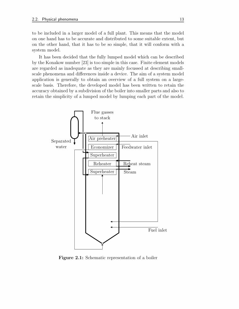
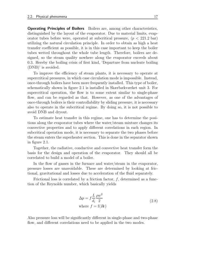
Figure 2.1: Schematic representation of a boiler
14 2. Basis for the Study of Boiler Dynamics
Looking at the boiler in figure 2.1, it may logically be divided into basicparts, such as combustion, furnace and superheater/reheater section. Themain phenomena to describe from a viewpoint of overall heat transfer is
• combustion
• heat transfer from flame to waterwalls
• heat transfer through waterwalls to water inside pipes
• heat transfer from flue gas through pipes to steam in superheater/re-heaters
• pressure loss in water, steam and flue gas.
2.2.2 Combustion Modelling
Basically, it takes fuel and oxygen to have a combustion. Under the rightcircumstances, i.e., sufficient temperature, mixing and residence time, thetwo will react by an, on the overall, exothermic process and establish theheat source in the boiler. When modelling the combustion, it is necessary todistinguish between the combustion of coal, oil and gas.
The simplest combustion reaction is present for gas, because the reactionis homogeneous and fast. The reaction speed is to a high extent only limitedby the mixing of fuel and oxygen, so ‘mixing equals combustion’ [40].
The boiler of Skærbækværket Unit 3 is fuelled by natural gas. For thisstudy it is assumed, that the time needed for combustion is negligible, andthat the intermediate products of the reaction do not have significant influ-ence on the heat transfer in the boiler.
Oil and especially coal consists of more complex molecules. Oil is in-troduced through atomizers and the combustion is a homogeneous reaction.For coal which is a solid, pyrolysis and gasification are intermediate steps inthe combustion. Gorner [40] gives equations for the estimation of the timeneeded for complete combustion of oil and coal.
2.2.3 Furnace Model
Heat transfer from the flame will mainly be due to radiation. The radiationmay be divided in grey-body radiation from a flame and gas radiation fromthe combustion products. The two modes of radiation are distinguished bythe type of flame originating from a given fuel. A flame acting as a body,i.e., absorbing, emitting and reflecting but not transmitting radiation, will
2.2. Physical phenomena 15
be present for combustion of fuels consisting of complex molecules, becausethese fuels form soot and also may consist of solid particles [23]. For greybody radiation in a furnace the total incident radiation to a wall, i, in anenclosure with N surfaces will be governed by a relation of the type:
Qi = Aiσ(N∑j=1
FijεjT4j + Fif εfT
4f ) (2.1)
Natural gas, which consists primarily of methane, will have a low tendencyto form soot in combustion [23, 89]. In gas combustion the flame will notact as a body, but as a mixture of hot gases, which will absorb, emit andtransmit radiation, but will not reflect it. The total incident radiation to awall, i, in an N -surface enclosure will be governed by a model of the form:
Qi = Aiσ(
N∑j=1
τjiFijεjT4j + εgT
4f ) (2.2)
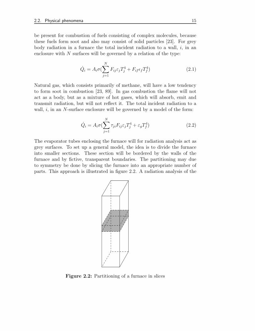
The evaporator tubes enclosing the furnace will for radiation analysis act asgrey surfaces. To set up a general model, the idea is to divide the furnaceinto smaller sections. These section will be bordered by the walls of thefurnace and by fictive, transparent boundaries. The partitioning may dueto symmetry be done by slicing the furnace into an appropriate number ofparts. This approach is illustrated in figure 2.2. A radiation analysis of the
Figure 2.2: Partitioning of a furnace in slices
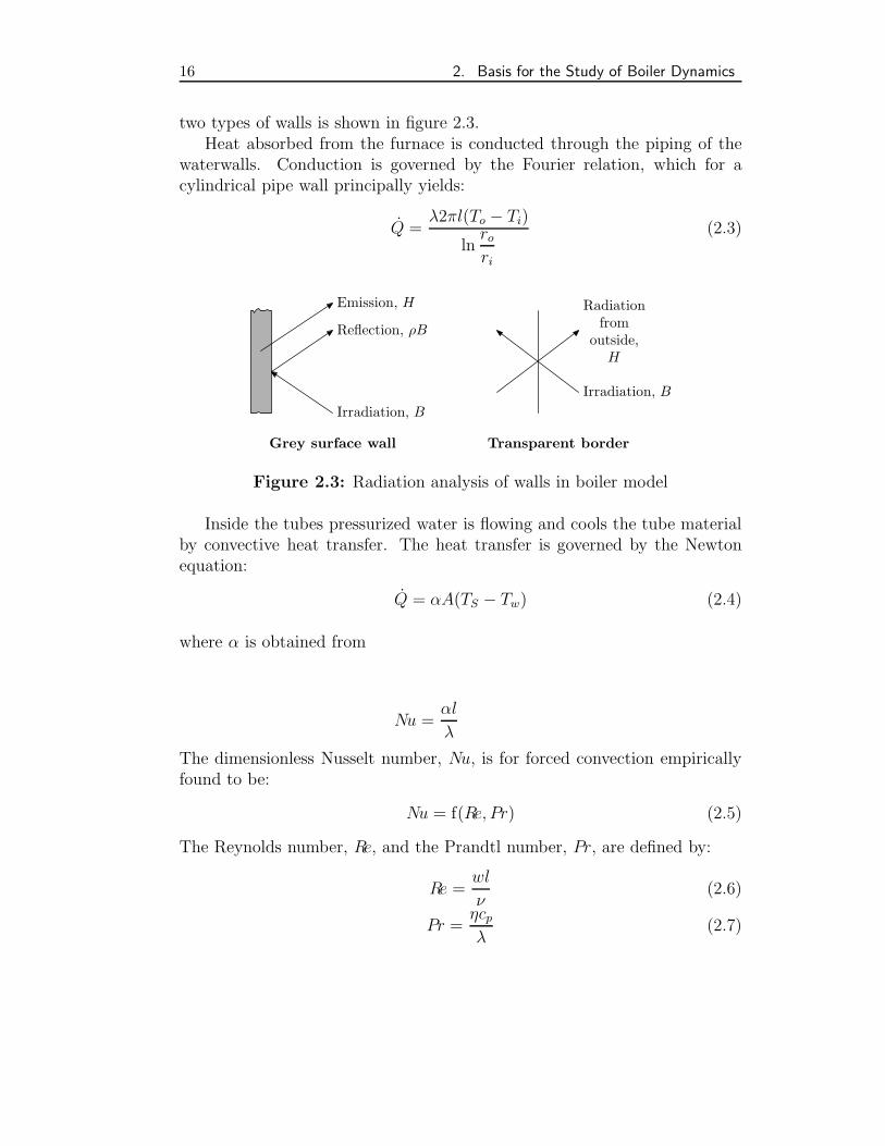
16 2. Basis for the Study of Boiler Dynamics
two types of walls is shown in figure 2.3.Heat absorbed from the furnace is conducted through the piping of the
waterwalls. Conduction is governed by the Fourier relation, which for acylindrical pipe wall principally yields:
Q =λ2πl(To − Ti)
lnrori
(2.3)
Irradiation, B
Reflection, ρB
Emission, H
Grey surface wall
Irradiation, B
Radiationfrom
outside,H
Transparent border
Figure 2.3: Radiation analysis of walls in boiler model
Inside the tubes pressurized water is flowing and cools the tube materialby convective heat transfer. The heat transfer is governed by the Newtonequation:
Q = αA(TS − Tw) (2.4)
where α is obtained from
Nu =αl
λ
The dimensionless Nusselt number, Nu, is for forced convection empiricallyfound to be:
Nu = f(Re, Pr) (2.5)
The Reynolds number, Re, and the Prandtl number, Pr, are defined by:
Re =wl
ν(2.6)
Pr =ηcpλ
(2.7)
2.2. Physical phenomena 17
Operating Principles of Boilers Boilers are, among other characteristics,distinguished by the layout of the evaporator. Due to material limits, evap-orator tubes before were, operated at subcritical pressure, (p < 221.2 bar)utilizing the natural circulation principle. In order to obtain as high a heattransfer coefficient as possible, it is in this case important to keep the boilertubes wetted throughout the whole tube length. Therefore, boilers are de-signed, so the steam quality nowhere along the evaporator exceeds about0.3. Hereby the boiling crisis of first kind, ‘Departure from nucleate boiling(DNB)’ is avoided.
To improve the efficiency of steam plants, it is necessary to operate atsupercritical pressures, in which case circulation mode is impossible. Instead,once-through boilers have been more frequently installed. This type of boiler,schematically shown in figure 2.1 is installed in Skærbækværket unit 3. Forsupercritical operation, the flow is to some extent similar to single-phaseflow, and can be regarded as that. However, as one of the advantages ofonce-through boilers is their controllability by sliding pressure, it is necessaryalso to operate in the subcritical regime. By doing so, it is not possible toavoid DNB and dryout.
To estimate heat transfer in this regime, one has to determine the posi-tions along the evaporator tubes where the water/steam mixture changes itsconvective properties and to apply different correlations in each region. Insubcritical operation mode, it is necessary to separate the two phases beforethe steam enters the superheater section. This is done in the separator shownin figure 2.1.
Together, the radiative, conductive and convective heat transfer form thebasis for the design and operation of the evaporator. They should all becorrelated to build a model of a boiler.
In the flow of gasses in the furnace and water/steam in the evaporator,pressure losses are unavoidable. These are determined by looking at fric-tional, gravitational and losses due to acceleration of the fluid separately.
Frictional loss is correlated by a friction factor, f , determined as a func-tion of the Reynolds number, which basically yields
∆p = fL
di
ρw2
2
where f = f(Re)
(2.8)
Also pressure loss will be significantly different in single-phase and two-phaseflow, and different correlations need to be applied in the two modes.
18 2. Basis for the Study of Boiler Dynamics
2.2.4 Superheater Section Model
The superheater sections are positioned after the furnace along the way ofthe gas flow in the boiler. The boiler in figure 2.1 is shown to have onepass having the superheaters above the furnace, but boilers may have morepasses to keep the construction lower. The superheaters may be designedfor radiative or convective heat transfer or a combination of both on thegas side. Radiative heat transfer will mainly be favoured in the superheatersections positioned immediately after the furnace where the gasses are at ahigh temperature. To maintain heat transfer in off-design operation, the useof both types of superheaters may be favourable [23].
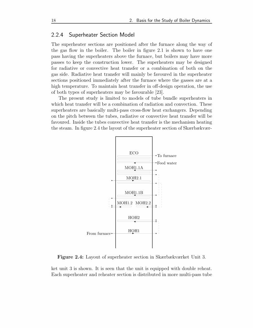
The present study is limited to models of tube bundle superheaters inwhich heat transfer will be a combination of radiation and convection. Thesesuperheaters are basically multi-pass cross-flow heat exchangers. Dependingon the pitch between the tubes, radiative or convective heat transfer will befavoured. Inside the tubes convective heat transfer is the mechanism heatingthe steam. In figure 2.4 the layout of the superheater section of Skærbækvær-
HOH1From furnace
HOH2
MOH2.2MOH1.2
MOH1.1B
MOH2.1
MOH1.1AFeed water
To furnaceECO
Figure 2.4: Layout of superheater section in Skærbækværket Unit 3.
ket unit 3 is shown. It is seen that the unit is equipped with double reheat.Each superheater and reheater section is distributed in more multi-pass tube
2.2. Physical phenomena 19
bundles. Each section has the bundles with highest temperature of steamplaced nearest the furnace.
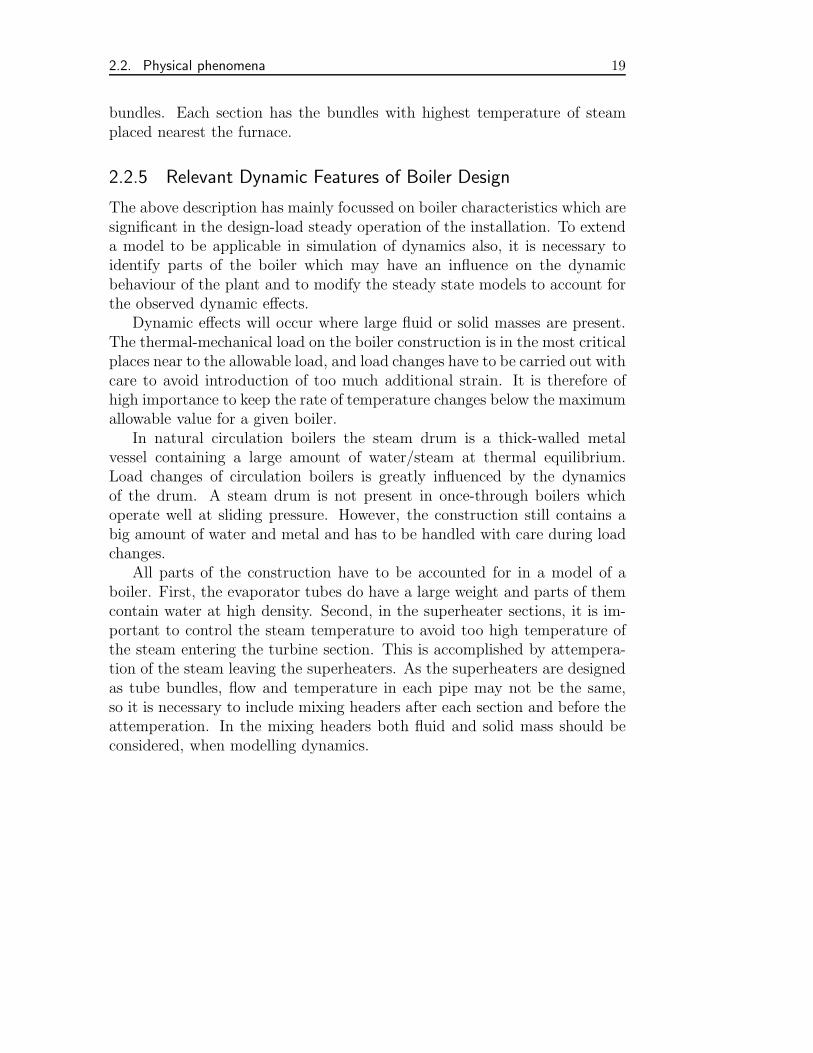
2.2.5 Relevant Dynamic Features of Boiler Design
The above description has mainly focussed on boiler characteristics which aresignificant in the design-load steady operation of the installation. To extenda model to be applicable in simulation of dynamics also, it is necessary toidentify parts of the boiler which may have an influence on the dynamicbehaviour of the plant and to modify the steady state models to account forthe observed dynamic effects.
Dynamic effects will occur where large fluid or solid masses are present.The thermal-mechanical load on the boiler construction is in the most criticalplaces near to the allowable load, and load changes have to be carried out withcare to avoid introduction of too much additional strain. It is therefore ofhigh importance to keep the rate of temperature changes below the maximumallowable value for a given boiler.
In natural circulation boilers the steam drum is a thick-walled metalvessel containing a large amount of water/steam at thermal equilibrium.Load changes of circulation boilers is greatly influenced by the dynamicsof the drum. A steam drum is not present in once-through boilers whichoperate well at sliding pressure. However, the construction still contains abig amount of water and metal and has to be handled with care during loadchanges.
All parts of the construction have to be accounted for in a model of aboiler. First, the evaporator tubes do have a large weight and parts of themcontain water at high density. Second, in the superheater sections, it is im-portant to control the steam temperature to avoid too high temperature ofthe steam entering the turbine section. This is accomplished by attempera-tion of the steam leaving the superheaters. As the superheaters are designedas tube bundles, flow and temperature in each pipe may not be the same,so it is necessary to include mixing headers after each section and before theattemperation. In the mixing headers both fluid and solid mass should beconsidered, when modelling dynamics.

20 2. Basis for the Study of Boiler Dynamics
3. DEVELOPMENT OF THE DNACODE
Turning the focus from a general model formulation to the formulation of amathematical model to be implemented in a simulator implies, that the modelhas to be formulated according to the requirements of the simulator. Thisnaturally confines the independency and the portability of the model. Oneway to limit the consequences of this confinement is to select the simulatorcarefully. It should not limit the extendability of the model during furtherdevelopments, and it should allow users to implement additional requiredfeatures.
The DNA program has been selected not only due to its extendability,but also due to its numerical methods and other features obtained during itsimplementation according to the PREFUR framework. It has, however, alsobeen realized during the modelling process that some parts of the code neededfurther extension. This development was needed not only for implementationof new features, but also to generalize the applicability of the existing fea-tures. These necessary rectifications have also revealed some weaknesses ofthe code, because they have involved changes of the fundamental parts of it.To describe the changes to the code, it is necessary to give an introductionto the theory, the features and the implementation of DNA.
3.1 Underlying Theory of DNA
The first step has been to formulate a systematic approach to the systemsmodelling. It has been concluded that the network approach is beneficial forthe formulation of system models in a program. This methodology allowsthe engineer to formulate the system model in the ‘usual’ way and easilytranslate it to an input model for a program, and it allows the program tobe well structured and robustly implemented.
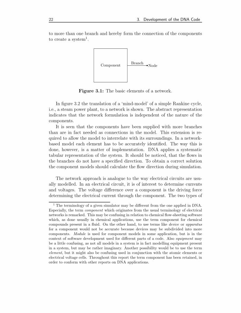
To convert a schematic diagram of a system to a network, each of thedevices is interpreted as a component with branches to its surroundings asshown in figure 3.1. The branches end at nodes. The nodes may be connected
22 3. Development of the DNA Code
to more than one branch and hereby form the connection of the componentsto create a system1.
Component BranchNode
Figure 3.1: The basic elements of a network.
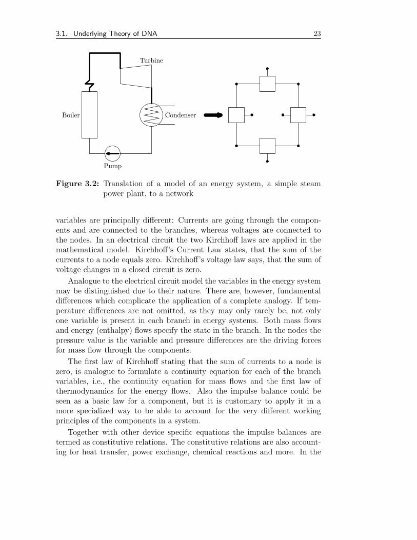
In figure 3.2 the translation of a ‘mind-model’ of a simple Rankine cycle,i.e., a steam power plant, to a network is shown. The abstract representationindicates that the network formulation is independent of the nature of thecomponents.
It is seen that the components have been supplied with more branchesthan are in fact needed as connections in the model. This extension is re-quired to allow the model to interrelate with its surroundings. In a network-based model each element has to be accurately identified. The way this isdone, however, is a matter of implementation. DNA applies a systematictabular representation of the system. It should be noticed, that the flows inthe branches do not have a specified direction. To obtain a correct solutionthe component models should calculate the flow direction during simulation.
The network approach is analogue to the way electrical circuits are usu-ally modelled. In an electrical circuit, it is of interest to determine currentsand voltages. The voltage difference over a component is the driving forcedetermining the electrical current through the component. The two types of
1 The terminology of a given simulator may be different from the one applied in DNA.Especially, the term component which originates from the usual terminology of electricalnetworks is remarked. This may be confusing in relation to chemical flow-sheeting softwarewhich, as done usually in chemical applications, use the term component for chemicalcompounds present in a fluid. On the other hand, to use terms like device or apparatusfor a component would not be accurate because devices may be subdivided into morecomponents. Module is used for component models in some application, but is in thecontext of software development used for different parts of a code. Also equipment maybe a little confusing, as not all models in a system is in fact modelling equipment presentin a system, but may be rather imaginary. Another possibility would be to use the termelement, but it might also be confusing used in conjunction with the atomic elements orelectrical voltage cells. Throughout this report the term component has been retained, inorder to conform with other reports on DNA applications.
3.1. Underlying Theory of DNA 23
Boiler
Turbine
Pump
Condenser
Figure 3.2: Translation of a model of an energy system, a simple steampower plant, to a network
variables are principally different: Currents are going through the compon-ents and are connected to the branches, whereas voltages are connected tothe nodes. In an electrical circuit the two Kirchhoff laws are applied in themathematical model. Kirchhoff’s Current Law states, that the sum of thecurrents to a node equals zero. Kirchhoff’s voltage law says, that the sum ofvoltage changes in a closed circuit is zero.
Analogue to the electrical circuit model the variables in the energy systemmay be distinguished due to their nature. There are, however, fundamentaldifferences which complicate the application of a complete analogy. If tem-perature differences are not omitted, as they may only rarely be, not onlyone variable is present in each branch in energy systems. Both mass flowsand energy (enthalpy) flows specify the state in the branch. In the nodes thepressure value is the variable and pressure differences are the driving forcesfor mass flow through the components.
The first law of Kirchhoff stating that the sum of currents to a node iszero, is analogue to formulate a continuity equation for each of the branchvariables, i.e., the continuity equation for mass flows and the first law ofthermodynamics for the energy flows. Also the impulse balance could beseen as a basic law for a component, but it is customary to apply it in amore specialized way to be able to account for the very different workingprinciples of the components in a system.
Together with other device specific equations the impulse balances aretermed as constitutive relations. The constitutive relations are also account-ing for heat transfer, power exchange, chemical reactions and more. In the
24 3. Development of the DNA Code
constitutive relations fluid properties may often have influences. This meansthat thermodynamic property models are of fundamental importance in en-ergy system models.
Because of the above, the analogy between electrical circuits and ther-modynamic processes is limited, and the advantage of the network theory ismainly, that it provides a systematic methodology for the preliminary imple-mentation considerations of a simulator.
Turning from this very general formulation of the basic model character-istics, it is evident from experience and other implementations (see section3.10.2), that the formulation of the physical and mathematical model is notthat general and is actually determining for the implementation of the sim-ulator and for the formulation of the system model.
3.2 DNA Models
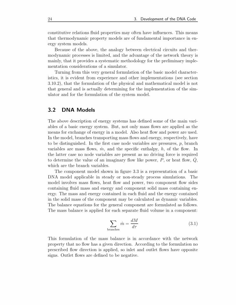
The above description of energy systems has defined some of the main vari-ables of a basic energy system. But, not only mass flows are applied as themeans for exchange of energy in a model. Also heat flow and power are used.In the model, branches transporting mass flows and energy, respectively, haveto be distinguished. In the first case node variables are pressures, p, branchvariables are mass flows, m, and the specific enthalpy, h, of the flow. Inthe latter case no node variables are present as no driving force is requiredto determine the value of an imaginary flow like power, P , or heat flow, Q,which are the branch variables.
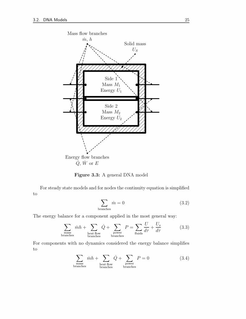
The component model shown in figure 3.3 is a representation of a basicDNA model applicable in steady or non-steady process simulations. Themodel involves mass flows, heat flow and power, two component flow sidescontaining fluid mass and energy and component solid mass containing en-ergy. The mass and energy contained in each fluid and the energy containedin the solid mass of the component may be calculated as dynamic variables.The balance equations for the general component are formulated as follows.The mass balance is applied for each separate fluid volume in a component:
∑branches
m =dM
dτ(3.1)
This formulation of the mass balance is in accordance with the networkproperty that no flow has a given direction. According to the formulation noprescribed flow direction is applied, so inlet and outlet flows have oppositesigns. Outlet flows are defined to be negative.
3.2. DNA Models 25
Side 1Mass M1
Energy U1
Side 2Mass M2
Energy U2
Energy flow branches
Q, W or E
Mass flow branchesm, h
Solid massUS
Figure 3.3: A general DNA model
For steady state models and for nodes the continuity equation is simplifiedto ∑
branches
m = 0 (3.2)
The energy balance for a component applied in the most general way:∑mass
branches
mh +∑
heat flowbranches
Q+∑power
branches
P =∑fluids
U
dτ+Us
dτ(3.3)
For components with no dynamics considered the energy balance simplifiesto ∑
massbranches
mh+∑
heat flowbranches
Q+∑power
branches
P = 0 (3.4)
26 3. Development of the DNA Code
In a node only one flow type is present, so the energy balance will be eitherof:
∑mass
branches
mh = 0 (3.5a)
∑heat flowbranches
Q = 0 (3.5b)
∑power
branches
P = 0 (3.5c)
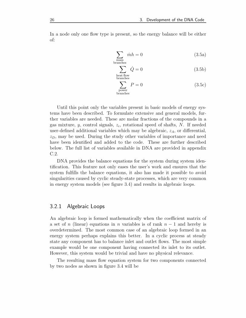
Until this point only the variables present in basic models of energy sys-tems have been described. To formulate extensive and general models, fur-ther variables are needed. These are molar fractions of the compounds in agas mixture, y, control signals, zc, rotational speed of shafts, N . If neededuser-defined additional variables which may be algebraic, zA, or differential,zD, may be used. During the study other variables of importance and needhave been identified and added to the code. These are further describedbelow. The full list of variables available in DNA are provided in appendixC.2.
DNA provides the balance equations for the system during system iden-tification. This feature not only eases the user’s work and ensures that thesystem fulfills the balance equations, it also has made it possible to avoidsingularities caused by cyclic steady-state processes, which are very commonin energy system models (see figure 3.4) and results in algebraic loops.
3.2.1 Algebraic Loops
An algebraic loop is formed mathematically when the coefficient matrix ofa set of n (linear) equations in n variables is of rank n − 1 and hereby isoverdetermined. The most common case of an algebraic loop formed in anenergy system perhaps explains this better. In a cyclic process at steadystate any component has to balance inlet and outlet flows. The most simpleexample would be one component having connected its inlet to its outlet.However, this system would be trivial and have no physical relevance.
The resulting mass flow equation system for two components connectedby two nodes as shown in figure 3.4 will be
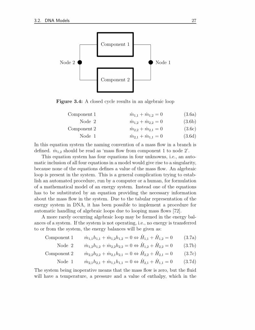
3.2. DNA Models 27
Component 1
Component 2
Node 1Node 2
Figure 3.4: A closed cycle results in an algebraic loop
Component 1 m1,1 + m1,2 = 0 (3.6a)
Node 2 m1,2 + m2,2 = 0 (3.6b)
Component 2 m2,2 + m2,1 = 0 (3.6c)
Node 1 m2,1 + m1,1 = 0 (3.6d)
In this equation system the naming convention of a mass flow in a branch isdefined. m1,2 should be read as ‘mass flow from component 1 to node 2’.
This equation system has four equations in four unknowns, i.e., an auto-matic inclusion of all four equations in a model would give rise to a singularity,because none of the equations defines a value of the mass flow. An algebraicloop is present in the system. This is a general complication trying to estab-lish an automated procedure, run by a computer or a human, for formulationof a mathematical model of an energy system. Instead one of the equationshas to be substituted by an equation providing the necessary informationabout the mass flow in the system. Due to the tabular representation of theenergy system in DNA, it has been possible to implement a procedure forautomatic handling of algebraic loops due to looping mass flows [72].
A more rarely occurring algebraic loop may be formed in the energy bal-ances of a system. If the system is not operating, i.e., no energy is transferredto or from the system, the energy balances will be given as:
Component 1 m1,1h1,1 + m1,2h1,2 = 0 ⇔ H1,1 + H1,2 = 0 (3.7a)
Node 2 m1,2h1,2 + m2,2h2,2 = 0 ⇔ H1,2 + H2,2 = 0 (3.7b)
Component 2 m2,2h2,2 + m2,1h2,1 = 0 ⇔ H2,2 + H2,1 = 0 (3.7c)
Node 1 m2,1h2,1 + m1,1h1,1 = 0 ⇔ H2,1 + H1,1 = 0 (3.7d)
The system being inoperative means that the mass flow is zero, but the fluidwill have a temperature, a pressure and a value of enthalpy, which in the
28 3. Development of the DNA Code
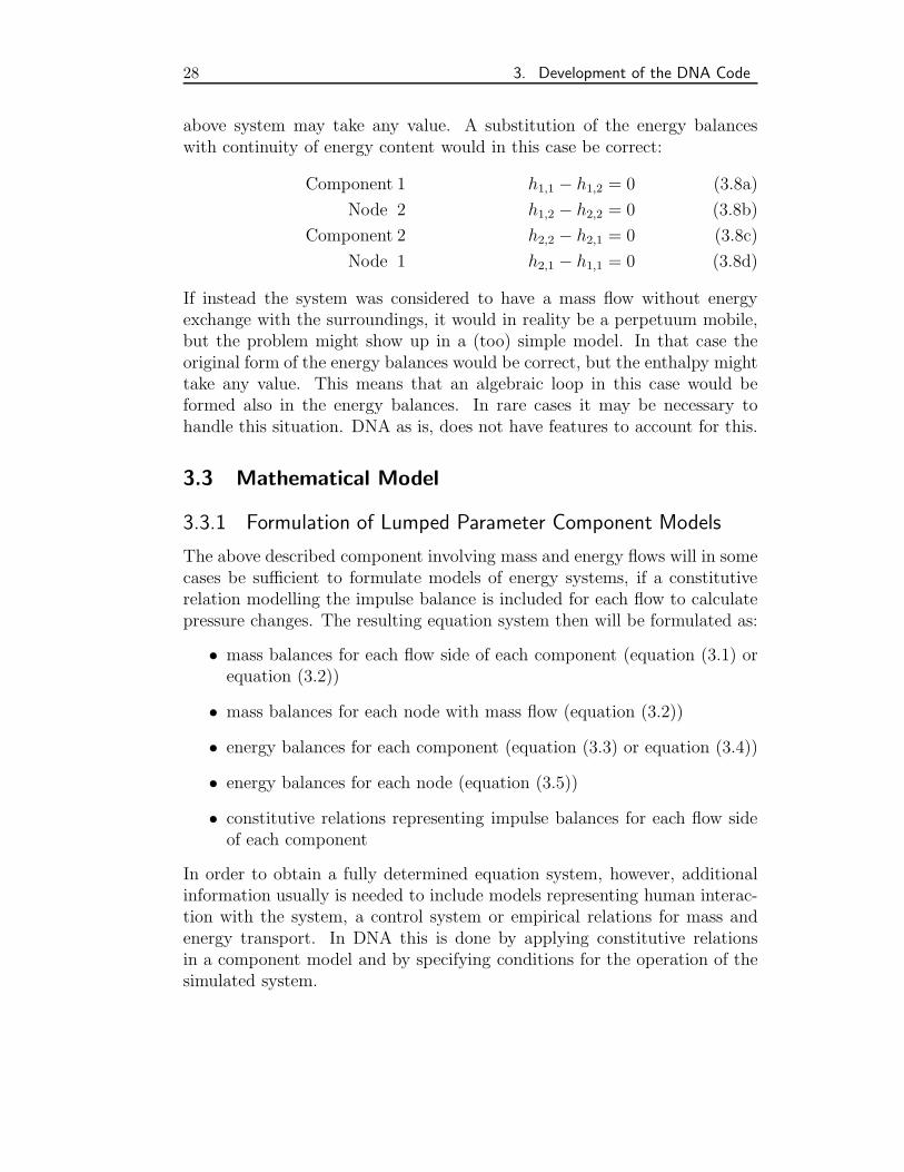
above system may take any value. A substitution of the energy balanceswith continuity of energy content would in this case be correct:
Component 1 h1,1 − h1,2 = 0 (3.8a)
Node 2 h1,2 − h2,2 = 0 (3.8b)
Component 2 h2,2 − h2,1 = 0 (3.8c)
Node 1 h2,1 − h1,1 = 0 (3.8d)
If instead the system was considered to have a mass flow without energyexchange with the surroundings, it would in reality be a perpetuum mobile,but the problem might show up in a (too) simple model. In that case theoriginal form of the energy balances would be correct, but the enthalpy mighttake any value. This means that an algebraic loop in this case would beformed also in the energy balances. In rare cases it may be necessary tohandle this situation. DNA as is, does not have features to account for this.
3.3 Mathematical Model
3.3.1 Formulation of Lumped Parameter Component Models
The above described component involving mass and energy flows will in somecases be sufficient to formulate models of energy systems, if a constitutiverelation modelling the impulse balance is included for each flow to calculatepressure changes. The resulting equation system then will be formulated as:
• mass balances for each flow side of each component (equation (3.1) orequation (3.2))
• mass balances for each node with mass flow (equation (3.2))
• energy balances for each component (equation (3.3) or equation (3.4))
• energy balances for each node (equation (3.5))
• constitutive relations representing impulse balances for each flow sideof each component
In order to obtain a fully determined equation system, however, additionalinformation usually is needed to include models representing human interac-tion with the system, a control system or empirical relations for mass andenergy transport. In DNA this is done by applying constitutive relationsin a component model and by specifying conditions for the operation of thesimulated system.
3.3. Mathematical Model 29
The following summary of quantities that may be of interest to obtainin a simulation of an energy system is supposed to be general, but as it isbased on experiences, mainly from the development of DNA, it may not besufficient for any kind of energy system. For instance plant types as nuclearplants, photovoltaic installations and fuel cells have not (yet) been studiedin this context.
Conditions Some conditions on flows, pressures or enthalpy may be re-quired to obtain the wanted information. According to the thermodynamicrelations between state variables, conditions on temperature, density, spe-cific volume, specific entropy, specific internal energy, or vapour fraction ofa gas-liquid mixture are equivalent to conditions on enthalpy.
Initial Values of Differential Variables Furthermore, if differential vari-ables are present, their values at the start of the simulation, i.e., initial val-ues, have to be specified. As before the thermodynamic state properties areequivalently applicable as conditions. Furthermore the time derivatives ofthe variables may be provided as conditions. More generally, any variable inthe system may supply sufficient information to solve the equation system atthe initial point in time. For fluid masses in the known internal volume of acomponent, the initial value may be specified from thermodynamic propertyvalues due to the hereby derived specific volume.
Constitutive Relations The application of specific values as conditions onvariables may not be sufficiently general to obtain the desired informationfrom a simulation of the model. This causes the need for formulation of moreconstitutive relations in a component model. These may for instance describespecified values of pressure losses or temperature differences, empirical re-lations for heat transfer or pressure loss, chemical reactions or separationprocesses. To include these relations in a model, it is necessary to introduceparameters which in component-based model formulations are lumping thecharacteristics of the components.
As chemical processes are present in many systems, constitutive relationsdescribing changes in composition of fluids and solid flows in a system arenecessary as options for a model.
Power production is most often maintained by an electrical generatorconnected to a shaft. The shaft will rotate at a given speed which dueto transients may be changing and hereby will be of interest to calculate.This is compared to other energy systems a special property in power plantengineering and need to be available in a simulator.
30 3. Development of the DNA Code
Additionally Calculated Variables In simulations there may turn out to bea need for knowledge of other quantities, such as heat fluxes or pressure losses,than those chosen to be the global variables in a system. These quantitiesmay also be derived by inclusion of additional constitutive relations in thesystem.
Another specialty that may be wanted is a possibility for calculation ofcomponent parameters from knowledge of a given state of a system. This isrelevant when correlating a model with given data for system operation.
Real systems usually have control systems, which may be modelled. Inthis case, error values and control signals have to be calculated and passedas information between components.
In figure 3.5 a component including all variables described above andhereby the most general possible component in DNA is shown. It can bededucted from this figure that a limitation in DNA is that only two separatecomponent flows may be included in a single component. The figure alsointroduces the naming of the variables as it is used throughout this thesis.In DNA the variables are accessed through key words. The list of key wordsis presented in appendix C.2.
3.3.2 Resulting System of Equations
The energy system model formulated by connection of component modelswill include all equations from each of the components. The variables of thesystem will, depending on the users selection of model equation, be eitheralgebraic or differential. For a steady state model all variables will be al-gebraic. If one or more variables are considered to show dynamic effects, adynamic model is formulated. Due to the applied formulation of the com-ponent models, node variables are assumed to be infinitely fast respondingto changes, and therefore always are algebraic. As a result, a dynamic modelof an energy system is a differential-algebraic equation system, a DAE.
3.4 Numerical Methods in Simulators
The above described formulation of a lumped parameter system model isgenerally applicable. To translate the mathematical model of the physicalsystem into a form readable by a computer program applied for solving thesystem, i.e., a numerical model, the model should be formulated in a waywhich conforms with the program. In any simulator a solution method for thenumerical model is applied. The available numerical methods are numerous
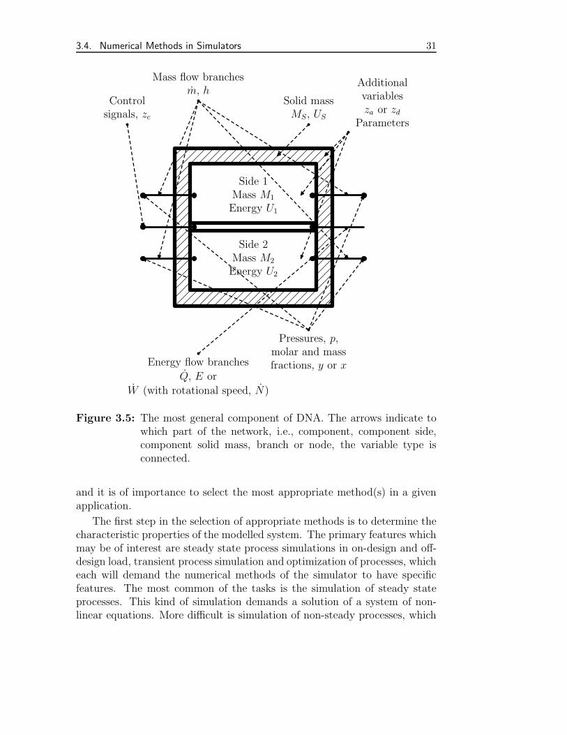
3.4. Numerical Methods in Simulators 31
Side 1Mass M1
Energy U1
Side 2Mass M2
Energy U2
Energy flow branches
Q, E or
W (with rotational speed, N)
Mass flow branchesm, h
Solid massMS, US
Pressures, p,molar and massfractions, y or x
Controlsignals, zc
Additionalvariablesza or zd
Parameters
Figure 3.5: The most general component of DNA. The arrows indicate towhich part of the network, i.e., component, component side,component solid mass, branch or node, the variable type isconnected.
and it is of importance to select the most appropriate method(s) in a givenapplication.
The first step in the selection of appropriate methods is to determine thecharacteristic properties of the modelled system. The primary features whichmay be of interest are steady state process simulations in on-design and off-design load, transient process simulation and optimization of processes, whicheach will demand the numerical methods of the simulator to have specificfeatures. The most common of the tasks is the simulation of steady stateprocesses. This kind of simulation demands a solution of a system of non-linear equations. More difficult is simulation of non-steady processes, which
32 3. Development of the DNA Code
will involve the solution of a system of differential or differential-algebraicequations. Optimization may be done for both steady and transient processesand will in any case involve a number of simulations of the system anddetermination of the most feasible configuration of the system. Optimizationand methods applied in this field are only briefly mentioned in the presentstudy.
Having determined which features are needed in the program, it is a mat-ter of wishes for generality, efficiency, availability, robustness and simplicityto select the most appropriate method and the most appropriate implement-ation of the selected method.
3.4.1 Methodology for Solution of Equation Systems
A mandatory feature of the program is a methodology applied when solv-ing the system of non-linear equations. The method may be selected amongmany possible according to the desired generality, simplicity, efficiency androbustness. The most simple way to treat the computation would be to re-quire the equations to be explicit, each determining the value of one variable.If allowed by the formulation of the equations it might be possible to calcu-late all variables in sequence and thereby obtain the wanted results. Thisapproach could be termed as explicit due to the formulation of the equationsand sequential due to the method applied in simulation. A simple modelof an open cycle, for instance a gas turbine, may be simulated using thisapproach. However, the applicability and generality of such an approach ishighly limited. With modifications, it may be much more relevant.
One modification which is required for simulation of closed cycles, is tointroduce a tear stream at which the same variables are applied at both sidesof the cut. The application of tear streams is similar to the way to handlealgebraic loops in sequential solvers. An iterative solution of the sequen-tial system may be done until the tear-stream variables have converged. Ifthe formulation of the equations is changed, so the equations belonging toeach device are identified as being a component model, a component-orientedcontrary to an equation-oriented approach is taken.
The equations may be formulated implicitly and hereby allowing themodel to be more general. Emphasizing the implicit formulation in a generalmethodology a simultaneous equation solver has to be utilized. Such solversare numerous and are available in various codes. Simultaneous solvers aredue to their general applicability isolated from the system model and maytherefore seem unappealing. The advantages of general equation system solv-ers is, that their properties are known and this make them easier to select fora given purpose. Also the extendability of a code based on a simultaneous
3.5. Numerical Methods of DNA 33
solver may be better.In some applications it has been decided to implement the numerical
solution procedure as a combination of sequential and simultaneous meth-odologies. This approach may provide the desired solutions and possess thewanted features, but it will on the other hand unavoidably introduce a lackof knowledge about the numerical properties of the method.
3.4.2 Methodology for Solution of Differential Equations
In simulation of systems involving transient processes, a solver for differentialequations is needed. The important problem in this context is, that time is anindependent variable and that a way to advance time during the simulationwhile retaining a correct solution, is needed.
A very simple approach to this problem may be to neglect dynamic effectsand simulate the steady-state model subject to time-varying conditions atconsecutive time steps. The main advantage of this approach is its simplicity,whereas it does not give any information about the accuracy of the solutionmethod. Knowledge about the solution is realized to be important for theapplication to models of energy systems which are often stiff. A DAE-systemis by definition infinitely stiff.
The way the lumped models have been formulated results in a semi-explicit index-1 DAE [72], i.e., the system of equations may be grouped indifferential and algebraic equations and may be written as
y′ = f(y, x, τ) (3.9a)
0 = g(y, x, τ) (3.9b)
in which x and y are algebraic and differential variables, respectively.That the actual formulation is implicit, and allows derivatives of more
variables in the same equation is considered not to change the characteristicsof the system. Thus a solver for this kind of DAE does apply [72]. Forthe semi-explicit index-1 case, a solver for ordinary differential equations isappropriate. The implicit formulation of the DAE may be written as
0 = f(y, y′, x, τ) (3.10a)
0 = g(y, x, τ) (3.10b)
3.5 Numerical Methods of DNA
Throughout the development of DNA, it has been of high importance torely on flexible and efficient methods. The selection of numerical methods
34 3. Development of the DNA Code
has been considered to be a crucial problem to handle correctly, because awell suited method and implementation provides good and well documentedproperties, as well as allowance for easier implementation of new features.
One characteristic to observe in energy system models is, that they oftencontain cyclic processes and due to that non-iterative methods will not beappropriate. To preserve generality of the simulator, it has been decided thatan implicit formulation of the component models is most appropriate, sinceit will allow one component model to be applied under various definitions ofthe conditions to which the system is subject. To obtain the most efficientcode, it has been realized that the most appropriate methods will be ofthe simultaneous kind. Of these the Newton method is well known and itsproperties are good [72].
3.6 The Modified Newton Method
For a non-linear system of equations given on residual or implicit form:
f(x) = 0 (3.11)
An iterative solution is obtained by determination of appropriate displace-ments of the variables in the system in each iteration step:
xi+1 = xi +∆xi+1, for i = 1, 2, 3... (3.12)
In order to start the method, the variables need to initialized before iterating.The method is successfully terminated when the residuals and displacementshave all converged to a value as close to zero as required by the user. Ifconvergence is not obtained within a maximum allowed number of iterationsor due to other problems, the method is divergent and is terminated withouthaving found a solution.
For the plain Newton method the displacements of the variables in aniteration are found from
Ji ·∆xi+1 = −f i (3.13)
where Ji is termed the Jacobian matrix. Its elements are evaluated as
Ji,j,k =∂f i,j∂xi,k
for j = 1, n and k = 1, n
The final convergence rate of the Newton method is quadratic, and it istherefore fast when this is obtained. On the other hand, the method is notrobust, because it will diverge if the system is not supplied with sufficiently
3.6. The Modified Newton Method 35
good initial guesses. In order to improve robustness of the method the firststeps may be damped, so only a fraction of the step is taken.
Another common modification of the method is to retain the same Jac-obian matrix for a number of iterations. This improves the speed of themethod, because the calculation of the Jacobian is time consuming.
The actual implementation of the method has some additional interestingfeatures.
3.6.1 Evaluation of the Jacobian Matrix
Evaluation of the Jacobian is crucial, because it is a computationally costlyoperation, either for the user or for the computer.
Principally, the Jacobian matrix could be evaluated from specified expres-sions for the partial derivatives of each equation with respect to each variable.This approach would, however, require a very large effort in algebra from themodeller, possibly involving differentiations of loops in thermodynamic prop-erty approximations which would not be easy.
The derivatives may instead be approximated by first order differencesbased on two evaluations of the equations. One is the value of the functionsat the actual point of the iterations. The other calculation is done at a pointa little away from the actual one. This second point is found by perturbingall variables relatively by a given fraction. If the value of a variable, j, iszero the perturbation, δj , is instead given an absolute value. The numericalapproximation to the derivative is given by:
∂f i∂xj
≈ f(xj)− f(xj + δj)
δj(3.14)
Because this method involves numerical evaluation of the equations, thesehave to be well-defined at any possible point, at which the solver may requirean evaluation. The equations, therefore, have to be formulated carefully.
To calculate the Jacobian matrix numerically, first an evaluation of themodel at the current point is required. In principle, a numerical evaluation ofthe Jacobian requires an additional number of model evaluations equal to thenumber of equations in the system. The number of evaluations may, however,be considerably reduced due to the formulation of energy system models ascomponent models. Often, only a few of the variables in the system influencea given component. For larger systems, this property is more pronounced,and the equation system is sparse. To make use of this property, the variablesmay be grouped, so none of the variables in one group is present in the sameequation, and accordingly does not affect the value of the same residual [17].
36 3. Development of the DNA Code
The application of this method in DNA is based on the assumption that allvariables connected to a component occur in each equation of the component[72]. This is a reasonable assumption even though some variables, in fact,are output and are only present in one equation.
If the grouping methodology is applied, the number of evaluations ofthe model is lowered to the maximum number of variables in one group.This will be the maximum number of variables influencing a component plusthe number of variables attached to the same nodes as the branches of thisparticular component. A system often includes a two-flow heat exchanger,with four branches connected to four nodes, as the component influenced bymost variables. In such a system, the smallest possible number of groupswill be 20, because each branch and each node holds two and one variables,respectively. This will be a typical number of groups, but if chemical reactionsare involved in the model, the number may be considerably higher.
Experienced Problems Empirically, it is found that there are a few mainsources for vulnerability of the applied method for evaluation of the Jacobian.One is that a mass flow may have a value of zero. If so, it will cause trouble inthe evaluation of the Jacobian matrix, because in many equations, the massflow is multiplied to enthalpy. If the mass flow is zero, an evaluation of thederivative of a given equation with respect to enthalpy, will be exactly zeroeven though the enthalpy is perturbed. In this case, a factorization of theJacobian will result in an error. In DNA, a (in some cases too) simple remedyof this problem has been made, by setting all mass flows to a non-zero valuewhen initializing the solver. However, if the mass flow does have a value ofzero, it cannot easily be handled by DNA. This problem need to be studiedfurther.
Another thing to take care of is that the value of enthalpy for a mixtureof ideal gasses is highly dependent on the composition, because enthalpy offormation is very different for different gasses. If some gas components areinitialized with a non-zero value, but are not present in the correct solution,or the opposite, it may happen that the solver is not able to determine propervalues of the derivatives in order to make the method converge.
Other Approaches to the Evaluation of the Jacobian Another approachwhich seems interesting is computational or automatic differentiation as de-scribed in [57, 104]. This methodology makes it possible for a program todifferentiate an equation possibly involving loops and branches. However, itwill require access to the source code of the model and will therefore probablynot be efficient compared to the numerical approximation calculated in the
3.6. The Modified Newton Method 37
compiled program. To have a correct Jacobian at any point, however, theapproach seems to be interesting.
For comparison [57] has found an optimal number of evaluations neededfor the automatic differentiation approach to be approximately the numberof equations times 2.5, which is indeed small compared to the number re-quired for numerical differentiation. Not considering the difference betweenevaluation of compiled and source code, the time savings by application ofautomatic differentiation is about 85–90%. The speed of evaluation of equa-tions in text input will be dependent on the implementation of a compiler orparser in the simulator.
3.6.2 Controlling the Update of the Jacobian Matrix
The Newton method may be modified to improve efficiency, by using someapproximation to the Jacobian, because it is time consuming to calculate.DNA allows the method to do a user-specified number of iterations, six bydefault, without updating the Jacobian [72]. To improve the efficiency fur-ther, it has been found that for some systems, many more iterations canbe done without losing the convergence of the method. As each iterationonly requires one model evaluation, and an evaluation of the Jacobian alsoinvolves a factorization, many iterations may be performed in the time, ittakes to evaluate the Jacobian.
Comparison of the ratio between errors and between displacements of twosucceeding iterations makes it possible to allow the iterations to run as longas convergence is ‘good enough’. The experience is that for some systemseven steps which diverge a little may be allowed, still preserving the overallconvergence of the method. This approach has been implemented in DNA.
It is worth to mention, that a main reason for the cost of the Jacobianevaluation is, numerous iterative solutions of equations for thermodynamicstates. For water/steam properties, the IFC-66 formulation [95] is used inDNA. This ought to be substituted by the recently published IAPS-97 for-mulation [108], which is both faster and more accurate.
3.6.3 Initialization of the Method
In any iterative method variables have to be initialized. The initialization ofvariables in DNA has been a time consuming task because any variable hadto be initialized manually by the user. Also, the initialization was limitedto enthalpy values for any flow. The user then had to convert knowledgeabout other thermodynamic quantities to enthalpy before writing the model.For real fluids, this may result in problems if a flow is initialized at a given
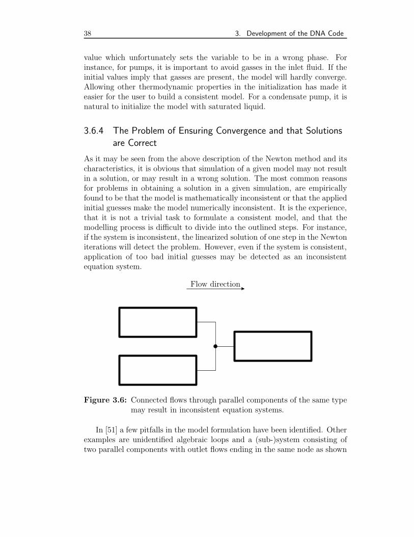
38 3. Development of the DNA Code
value which unfortunately sets the variable to be in a wrong phase. Forinstance, for pumps, it is important to avoid gasses in the inlet fluid. If theinitial values imply that gasses are present, the model will hardly converge.Allowing other thermodynamic properties in the initialization has made iteasier for the user to build a consistent model. For a condensate pump, it isnatural to initialize the model with saturated liquid.
3.6.4 The Problem of Ensuring Convergence and that Solutionsare Correct
As it may be seen from the above description of the Newton method and itscharacteristics, it is obvious that simulation of a given model may not resultin a solution, or may result in a wrong solution. The most common reasonsfor problems in obtaining a solution in a given simulation, are empiricallyfound to be that the model is mathematically inconsistent or that the appliedinitial guesses make the model numerically inconsistent. It is the experience,that it is not a trivial task to formulate a consistent model, and that themodelling process is difficult to divide into the outlined steps. For instance,if the system is inconsistent, the linearized solution of one step in the Newtoniterations will detect the problem. However, even if the system is consistent,application of too bad initial guesses may be detected as an inconsistentequation system.
Flow direction
Figure 3.6: Connected flows through parallel components of the same typemay result in inconsistent equation systems.
In [51] a few pitfalls in the model formulation have been identified. Otherexamples are unidentified algebraic loops and a (sub-)system consisting oftwo parallel components with outlet flows ending in the same node as shown
3.6. The Modified Newton Method 39
in figure 3.6. If the components are of the same type they will hold the sameequations and both may apply a constant pressure loss. This is naturallyimpossible and special care should be taken in this case. The easiest wayto overcome the problem is to include a free expansion (a reduction valve)between one of the components and the connection.
The reason for this kind of problems, however, is more fundamental, andhas to do with the application of component models which for modellingsimplicity, occur to be too simple under special conditions. It is important torealize this fact, but it may be overseen during a model formulation, becausethe component models are based on mathematical models, which may notbe well-behaved for any numerical value.
Another fundamental error which may be committed is to apply condi-tions which are not physically justified. This may result in, that the condi-tions together with the equations form an inconsistent system. Such errorsmay be hard to detect.
There are ways to let a program analyze a system and to divide it intosmaller parts which then may be assessed to determine what the problemis [80]. This approach seems interesting, but it will also be computationallycostly, and will involve additional manipulations not needed for the solutionof the system. Furthermore, the reason for the problem is application of awrongly formulated model and its solution is the users’ problem. He shouldformulate a physically correct, and mathematically and numerically consist-ent model. Since the user presumably has some experience in modelling ofenergy systems, it should be a tolerable task to make the model consistent.
Adjusted Damping of the Newton Method A simple generalization of theNewton Method has been investigated and has been found not to be robust.The idea was to apply damping to a step of the Newton Method to ensure,that it does not make the model enter an illegal region. A model, which dueto its simplicity, has been of major concern because it easily causes troublefor a solver is a counterflow heat exchanger with heat transfer coefficient, U ,and surface area, A, assumed to be constant and with given inlet conditionson both sides. The heat exchange will be governed by an expression involvingthe log mean temperature difference, ∆Tlm:
mc(hc,o − hc,i) = mh(hh,i − hh,o) = UA∆Tlm
where ∆Tlm =(th,i − tc,o)− (th,o − tc,i)
ln(th,i − tc,o)
(th,o − tc,i)
(3.15)
The temperature profile of this component is shown in figure 3.7. The tem-perature difference at the end with the lowest temperature difference will
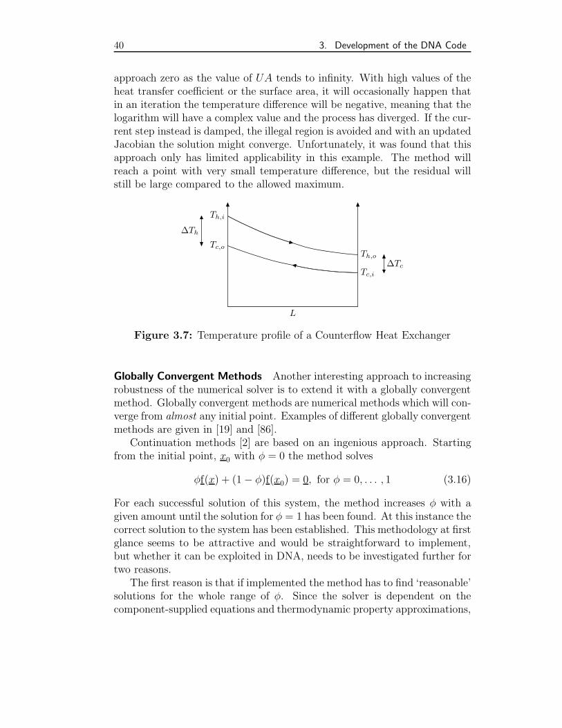
40 3. Development of the DNA Code
approach zero as the value of UA tends to infinity. With high values of theheat transfer coefficient or the surface area, it will occasionally happen thatin an iteration the temperature difference will be negative, meaning that thelogarithm will have a complex value and the process has diverged. If the cur-rent step instead is damped, the illegal region is avoided and with an updatedJacobian the solution might converge. Unfortunately, it was found that thisapproach only has limited applicability in this example. The method willreach a point with very small temperature difference, but the residual willstill be large compared to the allowed maximum.
L
Th,o
Tc,i
Th,i
Tc,o
∆Th
∆Tc
Figure 3.7: Temperature profile of a Counterflow Heat Exchanger
Globally Convergent Methods Another interesting approach to increasingrobustness of the numerical solver is to extend it with a globally convergentmethod. Globally convergent methods are numerical methods which will con-verge from almost any initial point. Examples of different globally convergentmethods are given in [19] and [86].
Continuation methods [2] are based on an ingenious approach. Startingfrom the initial point, x0 with φ = 0 the method solves
φf(x) + (1− φ)f(x0) = 0, for φ = 0, . . . , 1 (3.16)
For each successful solution of this system, the method increases φ with agiven amount until the solution for φ = 1 has been found. At this instance thecorrect solution to the system has been established. This methodology at firstglance seems to be attractive and would be straightforward to implement,but whether it can be exploited in DNA, needs to be investigated further fortwo reasons.
The first reason is that if implemented the method has to find ‘reasonable’solutions for the whole range of φ. Since the solver is dependent on thecomponent-supplied equations and thermodynamic property approximations,
3.6. The Modified Newton Method 41
difficulties may occur if the solution to the system is not in a valid region inthese models. Due to the nature of the mathematical model, the problem isto solve a system of constrained, non-linear equations. There has not beenfound a general numerical method for this kind of problem. Thus the modelshave to be made unconstrained.
The second reason is as above, that convergence problems usually occurdue to application of too bad user-supplied initial values. These may beavoided because the system is known to be an energy system in which thebalance equations have to be fulfilled. This has been exploited in DNAduring this project to generate good initial values. This approach has madethe simulation much easier convergent, and a better solver is no longer sorelevant.
3.6.5 Generation of Initial Guesses
Generation of good initial guesses for the variables has two purposes. Con-vergence of the method will be much more likely and the user’s work inpreparation of the input file is highly diminished and is more focussed on theformulation of a proper model. In appendix E, the size of input files withand without initial guesses supplied by the user are compared. It is hereseen that the amount of work required from the user is much lower with theminimal number of initial guesses applied.
The methodology applied for generation of initial guesses is based on afirst principles analysis of the system and does not include any numericalcalculations. In this way considerations about divergence of numerical meth-ods have been avoided. On the other hand, this approach restricts the users’choice of input to the model, because mass balances are given higher priorityand have to be fulfilled for a component before an attempt to set up the firstlaw is made.
First step in the generation of initial guesses is to transfer the appliedconditions to be used as initial guesses also. This will provide a basis forthe further generation of the array of initial guesses. Next, this knowledgeabout pressure, mass flow and enthalpy or energy flow in one branch, maybe used to extend the initial guesses to branches directly connected to thesame component.
For pressures, which are node variables, the extension is based on anassumption of constant pressure through components. To keep the initializ-ations reasonable, it has therefore been necessary to omit extension of pres-sures over components with power input or production. These componentswill generally be compressors, pumps or turbines and will therefore involvelarge pressure changes which cannot be predicted without ‘looking inside’ of
42 3. Development of the DNA Code
the component and hereby require numerical calculations during the initial-ization.
For the branches, both mass flow and enthalpy or energy flow, respect-ively, should be initialized. This is done by application of mass and energybalances to the components and nodes. In this procedure mass balances,which are the simplest, take precedence such that, if a mass flow to or from acomponent has not been initialized, the energy balance is not set up. In thisway mass flows are required to be known before energy flows and enthalpiesare calculated. Naturally, to extend the array of initial guesses, all but one ofthe variables in a balance must have been initialized. To express the energybalance the medium in a node must be known. This means that compositionof gas mixtures must have been initialized to generate the guesses. In orderto avoid numerical calculations in the generation of the guesses, it has beendecided that the user has to specify the initial composition of all media in themodel. A nearly correct initial composition may in some cases be importantto make the solver converge.
After the initialization of variables entering the balances of nodes andcomponents, another approach to initialization of the additional variables ofthe system has been made possible. When modelling a component, it maybe relatively straightforward to formulate explicit expressions for additionalvariables and control signals. This has been allowed in a separate part of thecomponent routine (see appendix B).
It is noticed that any initial value specified in the users input take pre-cedence and will not be overruled by generated values. On the other hand,DNA do check if all variables have been initialized and will complain if anyvariable has not been assigned a value. Therefore, during model implement-ation, which is usually a stepwise extension of the system model, it may be agood practice to add new components without any additional initializationsand let the program request the needed information. In this manner, theprogram features for initialization will be best exploited.
Another issue to notice is that during model setup, it is possible to reusevariable values obtained in foregoing simulations of a model. Reusing sim-ulation results as initial guesses together with the above explained facilitiesmakes the setup of input files easier and less time consuming. Simulations ofmodels with very accurate initial guesses found in previous runs will be fastand easily convergent. The results of the previous simulation of an input fileare applied as initial guesses for the user-specified ones in a file.
As a last resort when the user is unable to figure out what causes aproblem, a debug file displaying the information in the internal tables ofDNA is generated by the program from the input. This file will also indicateif any condition in the system is violated when applying the initial guesses.
3.6. The Modified Newton Method 43
3.6.6 Generalization of Component Models
The generation of good initial guesses only remedies part of the problemwith non-convergence of the solution. The difficulty caused by equationsbeing mathematically undefined or having no physical relevance for somevariable values has not yet been taken care of.
As described in section 3.6.4 the Newton method may be supplementedby other globally convergent methods. These methods, however, are inten-ded for use with equations being (at least) continuous and unconstrained.Furthermore, the problem has its basis in the conception of modelling, dueto the formulation of a numerical model for a physical phenomenon. Thistranslation involves assumptions which may contradict physics. Therefore,it has been decided that the model has to account for avoidance of problemsdue to simplifications applied in its formulation.
The generalization of component models to avoid mathematically or phys-ically invalid regions will be based on branching of the problematic equationsof a model. If possible such branching should be made, so the equation willbe continuous and differentiable in the point of the branch, but it may beimpossible to do so. However, the modified Newton method works withapproximations to the Jacobian, as it is done in DNA.
The main issue to focus on, when generalizing the equations has empir-ically been found to be that the variables are forced to move back into theallowed region. Also, the equation system still has to be fully determinedalso in the wrong regions. Otherwise, an evaluation of the Jacobian in theseregions will cause the method to break down due to the impossibility offactorizing the Jacobian matrix.
Turbine Model A first simple example of generalization of numerical mod-els of devices is the flow in a turbine modelled by a turbine constant, CT .The lumped impulse balance of this model will be in the general form:
CT =mi
√Ti√
p2i − p2
o
(3.17)
which is only defined for T > 0 K and p2i > p2
o, and is furthermore only phys-ically relevant for pi ≥ 0 bar and po ≥ 0 bar. To make the model numericallymore general, it is convenient to formulate it as:
C2T (p
2i − p2
o) = m2iTi (3.18)
Hereby the variables may take any value. Unfortunately, some quantities aresquared causing the equation to be fulfilled for both negative and positive
44 3. Development of the DNA Code
values. To overcome this problem the squares may be reformulated by in-troduction of a branching which may be done applying the absolute value ofthe quantities as in:
|CT |CT (|pi|pi − |po|po) = |mi|miTi (3.19)
In this formulation the model will be robust and general and will not make thesolution procedure fail. The applied generalization ends up in a model stillbeing both continuous and differentiable. The next example shows that this isnot always a possibility, even though generalization of the model formulationis possible.
Counterflow Heat Exchanger The counterflow heat exchanger model (fig-ure 3.7) again serves well as a model which is difficult to handle. If the heattransfer equation of the model is evaluated in a region where the temperat-ure profiles cross, i.e., the temperature differences at the ends have oppositesigns, it is mathematically undefined and physically impossible. However,the variables may during iterations have entered this region, and the solvershould preferably handle this. If the model enters this region, it is mostprobably caused by a high heat transfer coefficient or surface area. Thismeans that in fact the temperature difference in one end should be close tozero, but should not be allowed to be negative. It has been found that a wayto handle this problem is to switch the heat transfer relation to a (simpler)temperature difference, explicitly requiring the solver to exit the forbiddenregion.
Q = UA∆Tlm, for ∆Tc ·∆Th > 0
∆Tc = δ, for ∆Tc ·∆Th ≤ 0 ∧ mccp,c < mhcp,h
∆Th = δ, for ∆Tc ·∆Th ≤ 0 ∧ mccp,c > mhcp,h
where δ is a small positive number
(3.20)
This formulation does not account for all situations. For instance if the heatcapacity flow is the same on both sides or the temperature difference is thesame at both ends, further extensions must be made. The presentation is onlyintended to show a principle for how successful generalizations of componentmodels can be carried out. More such robust components including the fullformulation of the counterflow heat exchanger is shown in chapter 4.
3.7 Solution of Differential-Algebraic Equation Systems
A brief introduction to the integration method applied in DNA is in place tomotivate the extensions which have been applied to it during this study. For
3.7. Solution of Differential-Algebraic Equation Systems 45
a thorough description of the method [72] should be consulted. DAEs andtheir solution are handled in [5].
The basic choice when selecting an integration routine is whether to usemulti-step methods or one-step methods. Multi-step methods will usually beof the BDF–kind, whereas single-step methods will be Runge–Kutta meth-ods. The system will be a semi-explicit index–1 DAE, and the BDF’s havebeen chosen to be most appropriate [72]. These methods may be implemen-ted in different ways depending on needed features and desired properties.
3.7.1 Nordsieck Formulation of BDF methods
On the usual multi-step form an integration step of a k–step BDF–methodmay be written as
k∑j=0
αjyn+j= hβkfn+k
in which f = f(y, y′, t) = y′(3.21)
The stability region for these methods decreases fast with the order, p, ofthe method which is equal to the number of steps for BDF’s. This has beenselected to be four, for which the stability region is reasonable.
To introduce a possibility for using variable step sizes, the Nordsieckformulation of the BDF method is introduced [72]. For each differentialvariable a Nordsieck vector, Y , is formed. Instead of storing the solutionpoints back in time, the Nordsieck vector stores the solution and its k firstderivatives, so only information about the last calculated point is needed.
Y i = [yi, hy′i,h2
2y′′i , . . . ,
hk
k!y
(k)i ]T (3.22)
A polynomial approximation to the solution will then correspond to a Taylorexpansion of the solution from the last calculated point. For ease of calcula-tion of this, it is assumed that the last k solution points are equidistant [87].This assumption is naturally not true when the formulation is to be usedwith a variable step size method. Due to this, it is necessary to require timestep changes to be smaller than a given limit, usually defined as a maximumratio between two succeeding time steps.
A change of the size of a time step only involves a multiplication of theratio between time steps, i.e., κ = hnew/h to the j’th power to each of theentries of the Nordsieck vector:
Y i = [yi, (κh)y′i,(κh)2
2y′′i , . . . ,
(κh)k
k!y
(k)i ]T (3.23)
46 3. Development of the DNA Code
Another prerequisite for a variable step size implementation is an estim-ation of the error of the method, i.e., the difference between the calculatedapproximation and the real solution. This is made possible by introductionof an explicit predictor defined by
k∑j=0
αjyn+j= hβk−1fn+k−1 (3.24)
The predicted value for a method may be found by a simple matrix operation:
Y Pn+1 = PY C
n (3.25)
where P is termed the Pascal Matrix and is defined by
P(i, j) =
0 , for i < k
1 , for i = k ∨ i = 1
P(i− 1, j) +P(i− 1, j − 1) , else
In general an estimate of the local truncation error of a variable is ex-pressed as:
etrun,i = CChp+1yp+1
i,n(3.26)
Provided that predictor equation (3.24) and corrector equation (3.21) areof the same order, the truncation error may be calculated using Milne’sestimate:
etrun,i =CC
CP − CC(yC
i,n− yP
i,n) (3.27)
The difference between the corrected and predicted Nordsieck vector may bewritten as lw, where w is a scalar. The l vector is usually normalized bysetting its second entry equal to one. Doing so the truncation error can beexpressed in a simple manner as:
etrun,i ∝ w (3.28)
These operations also make it possible to include the integration methodin the Newton solver which then includes equations for the differential vari-ables, their time derivatives and their error estimates. In order to simulatedynamics, the differential variables have to have a known value for the initialtime step.
3.7. Solution of Differential-Algebraic Equation Systems 47
3.7.2 Initialization of the Integration Method
To initiate a multi-step method, it is required to obtain a number of solutionpoints equal to the order of the method. This may be done either by using alower order multi-step method with the drawback of smaller step sizes or byusing single-step methods with the drawback of having to implement theseseparately. In DNA the first possibility has been used by implementing anincreasing order BDF which works well due to the variable step size method.
It should be noticed that the method is not implemented with ordercontrol. The truncation error of the method is given by equation (3.26). Theerror may be calculated for lower orders of the method in addition to theerror for the present method. Of these the one having the smallest errorshould be used for the following step. Doing so, it may be that the selectedmethod has a lower order, and thereby is both simpler to apply and is morestable, than the maximum order method implemented. An implementationof an order-selecting method seems to be an easy task for improvement ofthe numerical routines of DNA.
Any integration routine requires any differential variable of a model tohave a well-defined initial value. Usually and as the only possibility for ex-plicit integration routines, these values should be specified directly by theuser. For implicit integration routines, as the one employed in DNA, theway to specify the initial point for the model may be generalized, becausethe solution procedure at a given point does not need specific variables tohave a known value as long as the model has a solution. Generally, the modelcould be initialized by fixing any set of variables that allows the model tohave a well-defined solution, no matter if the variables are algebraic, differ-ential or derivatives thereof. Such a general approach has not, by now, beenimplemented in DNA, but a handy facility which allows the user to specifytime-derivatives of the differential variables instead of their value for the ini-tial solution has been included. The main purpose in applying this featureto a model is to require a model to be in a steady state when starting thesimulation. At some point it is then possible to change some values of themodel and introduce a transient process.
As for algebraic variables, also the initial values of differential variablesmay be obtained using any of the thermodynamic properties in DNA. Ifmass of fluid inside a component is considered to be dynamic, its initialvalue may be specified explicitly, by specific volume or it may be derivedfrom specified values of pressure for an ideal gas or for pressure and anotherthermodynamic property for a real fluid. If internal energy is differential, itis similarly possible to calculate the initial value from knowledge of pressureand another property.
48 3. Development of the DNA Code
3.7.3 Handling Discontinuities
During a simulation of a dynamic system, an equation or its derivatives maybe discontinuous between two discrete values of the independent variable(time). In such a situation special care has to be taken to preserve order ofthe applied method [49]. Discontinuities will most often arise from modelsof events due to intervention by human operators or a control system. Dis-continuities may be distinguished depending on whether they are defined ata given value of the independent variable, or if they are defined at a givenvalue of a dependent variable. An example of the first form is a process wherean operator changes a valve opening at a specified time. An example of thelatter is a valve which position is changed by the control system of a plant.
The BDF methods are based on polynomial (Taylor) expansions of eachvariable back in time. Due to this the integration method must be restartedat the passage of the discontinuity. Otherwise the approximation to thesolution would be wrong.
Discontinuities dependent on the independent variable only, are most easyto handle as they may be specified directly before the simulation begins. Theintegration hereby may be stopped and restarted exactly at the passage. Afeature to do so has been implemented in DNA by Lorentzen [72].
General discontinuities which may be dependent on any variable in thesystem are more difficult to handle because they have to be located, so theintegration routine is in fact stopped at the passage, but on the other hand isnot stopped before the passage which would cause at least one more restartwhen the discontinuity is reached again. General discontinuities, do includediscontinuities in both the equations themselves and in their derivatives.
According to [49] the best way to handle this situation correctly is tolocate the exact point of passage of the discontinuity and restart the integ-ration here, or more precisely right after. To locate the point in time wherethe equation is discontinuous an additional variable, i.e., a switch variable,which changes its sign at the passage of the discontinuity is introduced. Bycalculating the value of this variable, it is possible to detect the discontinuity.
In figure 3.8 an example of a discontinuous equation is displayed. Untilsome point the equation is continuous and smooth. At the point of thediscontinuity the equation switches from one branch, (left of the dashed line)to another (right of the dashed line). Indicated by zs− the graph of the switchvariable up to the discontinuity is displayed. As seen the switch variable atsome point passes from a positive value to a negative value. This changeof sign informs the integration routine that a discontinuity is about to bepassed and that the model is about to enter another state. The solver thenenters the procedure which locates the point of passage.
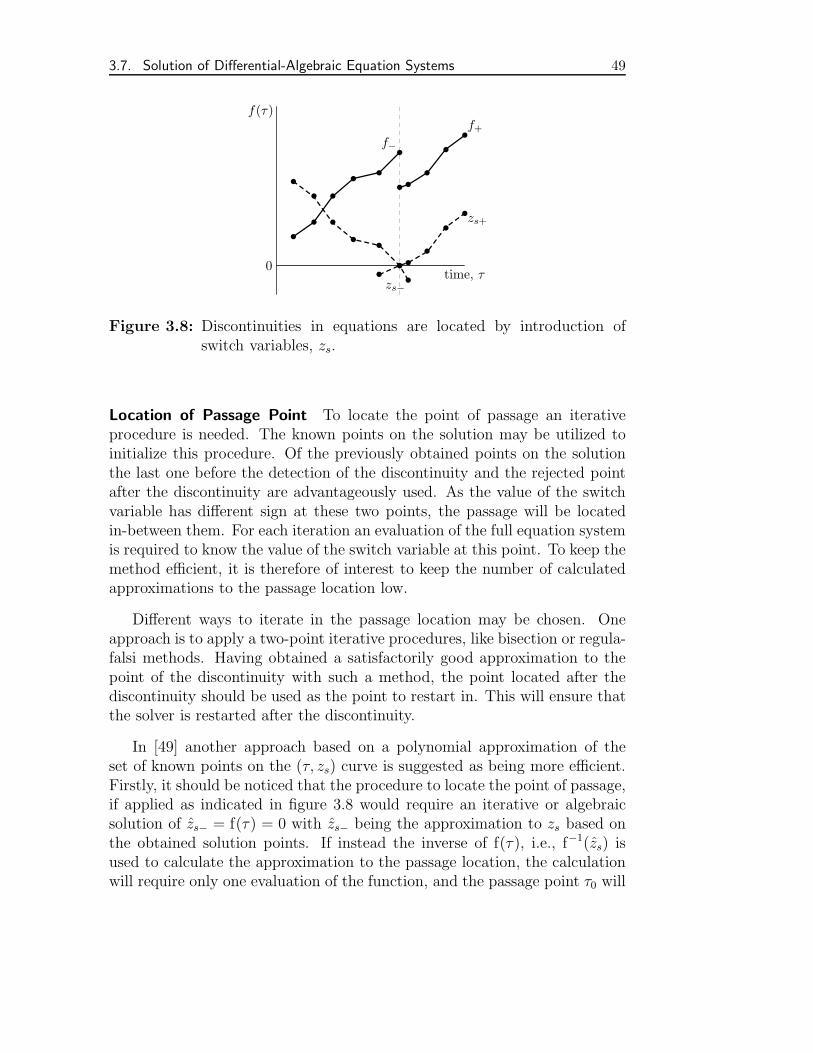
3.7. Solution of Differential-Algebraic Equation Systems 49
0
f−
zs−
f+
zs+
time, τ
f(τ)
Figure 3.8: Discontinuities in equations are located by introduction ofswitch variables, zs.
Location of Passage Point To locate the point of passage an iterativeprocedure is needed. The known points on the solution may be utilized toinitialize this procedure. Of the previously obtained points on the solutionthe last one before the detection of the discontinuity and the rejected pointafter the discontinuity are advantageously used. As the value of the switchvariable has different sign at these two points, the passage will be locatedin-between them. For each iteration an evaluation of the full equation systemis required to know the value of the switch variable at this point. To keep themethod efficient, it is therefore of interest to keep the number of calculatedapproximations to the passage location low.
Different ways to iterate in the passage location may be chosen. Oneapproach is to apply a two-point iterative procedures, like bisection or regula-falsi methods. Having obtained a satisfactorily good approximation to thepoint of the discontinuity with such a method, the point located after thediscontinuity should be used as the point to restart in. This will ensure thatthe solver is restarted after the discontinuity.
In [49] another approach based on a polynomial approximation of theset of known points on the (τ, zs) curve is suggested as being more efficient.Firstly, it should be noticed that the procedure to locate the point of passage,if applied as indicated in figure 3.8 would require an iterative or algebraicsolution of zs− = f(τ) = 0 with zs− being the approximation to zs based onthe obtained solution points. If instead the inverse of f(τ), i.e., f−1(zs) isused to calculate the approximation to the passage location, the calculationwill require only one evaluation of the function, and the passage point τ0 will
50 3. Development of the DNA Code
be:
τ0 = f−1(zs = 0) (3.29)
Application of a Nordsieck vector to each switch variable might be apossibility since this methodology is already used in the DNA. However, thisis not a beneficial method in this case, because the Taylor expansion of thevariables by interpolating polynomials is based on an assumption of constantstep size. Employing the inverse function, this assumption would require thechanges of the values of the switch variables to be limited and might introducerestrictions on the time step size in the ordinary integration routine.
Instead the divided differences has been found to be advantageous. Whena discontinuity is encountered a linear approximation to the passage point,τ0, can be found as:
τ0 = τ(zs,n) +τ(zs,n)− τ(zs,n−1)
zs,n − zs,n−1· zs,n (3.30)
where n and n − 1 indicate the point after and before the discontinuity,respectively. A better approximation to the passage point may hereby beobtained. The fraction in the right hand side of equation (3.30) is the firstof the divided differences used in the method. These are for a k’th orderpolynomial approximation from point n defined recursively by [67]:
τ [zs,n, . . . , zs,n−i] =τ [zs,n, . . . , zs,n−i+1]− τ [zs,n−1, . . . , zs,n−i]
zs,n − zs,n−i
with τ [zs,i] = τi, i = n− k, . . . , n
(3.31)
A polynomial approximation to τ = f−1(zs) based on these then is:
τ(Z) =τ [zs,n] + (Z − zs,n)τ [zs,n, zs,n−1] +
(Z − zs,n)(Z − zs,n−1)τ [zs,n, zs,n−1, zs,n−2] + . . .
(Z − zs,n) · . . . · (Z − zs,n−k+1)τ [zs,n, . . . , zs,n−k]
(3.32)
This approximation may be written in form of a Horner scheme [49]:
τ(Z) = τ [zn]+(Z − zs,n)
(τ [zs,n, zs,n−1] +
(Z − zs,n−1)(τ [zs,n, zs,n−1, zs,n−2] +
. . .+
(Z − zs,n−k+1)τ [zs,n, . . . , zs,n−k]))) . . .))
(3.33)
3.7. Solution of Differential-Algebraic Equation Systems 51
At the interesting point Z = 0 this simplifies to
τ0 = τ [zn]−zs,n(τ [zs,n, zs,n−1]−
zs,n−1
(τ [zs,n, zs,n−1, zs,n−2]−
. . .−zs,n−k+1τ [zs,n, . . . , zs,n−k]))) . . .
))(3.34)
By each iteration a new point on the curve may be introduced in the divideddifferences scheme allowing the approximation to be arbitrarily accurate.There has not been found a way to make this introduction easily, becausethe new point will have to be introduced at the correct point in the schemeand affects all other values calculated afterwards in the recursion. However,only very seldom a change of sign of more than one switch variable willoccur, depending on the model of course. This means that only one divideddifferences scheme has to be updated and efficiency of the method is retained.If more than one switch is detected an additional scheme will be required foreach.
The iteration is stopped when a value of the switch variable sufficientlynear to zero has been found. If the value of the switch variable is positiveat this point in time, the solution has not passed the discontinuity and somesteps should be taken until the discontinuity has been passed. These stepsshould be of the minimal allowed size to have the possibility to switch themethod exactly when the discontinuity is passed. To decide how precise theiterated value of the passage point should be, therefore requires a weighingof the accepted number of calculated solutions and the accepted numberof minimal steps taken. The experience is that the iterations should becontinued until a value very near to zero has been found, whereby the numberof minimal steps is minimized.
In figure 3.8 the switch variable is following another curve, zs+, after thediscontinuity. This indicates that the switch variable is described by anotherequation after the switch, because it is required, that the switch variableis always positive. The reason for not only detecting sign changes of theseequations is that by requiring the equation always to be positive, it is possibleto ensure that the model will be in the correct state at the initial time step,i.e., τ = 0.
Initialization of the Discontinuity Locating Procedure The initializationof the method may be carried out in two ways depending on the nature ofthe modelled system.
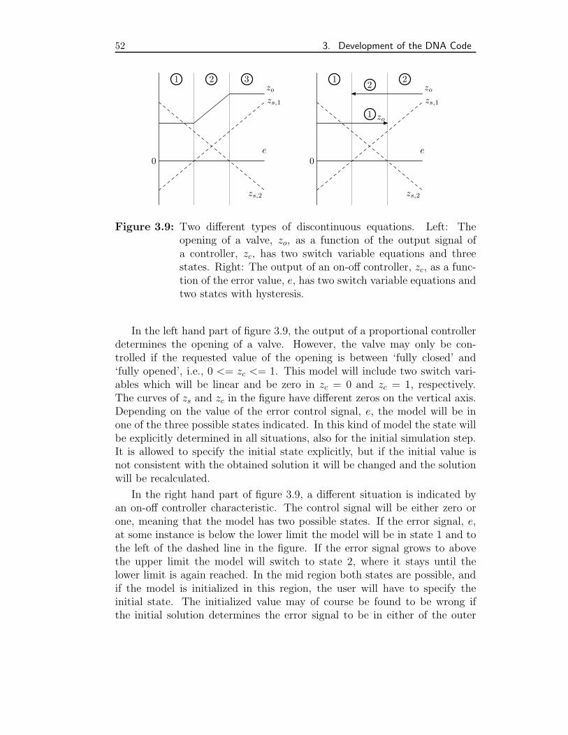
52 3. Development of the DNA Code
0
zs,1
zs,2
zo
e
1 2 3
0
zs,1
zs,2
zo
zo
e
1 22
1
Figure 3.9: Two different types of discontinuous equations. Left: Theopening of a valve, zo, as a function of the output signal ofa controller, zc, has two switch variable equations and threestates. Right: The output of an on-off controller, zc, as a func-tion of the error value, e, has two switch variable equations andtwo states with hysteresis.
In the left hand part of figure 3.9, the output of a proportional controllerdetermines the opening of a valve. However, the valve may only be con-trolled if the requested value of the opening is between ‘fully closed’ and‘fully opened’, i.e., 0 <= zc <= 1. This model will include two switch vari-ables which will be linear and be zero in zc = 0 and zc = 1, respectively.The curves of zs and zc in the figure have different zeros on the vertical axis.Depending on the value of the error control signal, e, the model will be inone of the three possible states indicated. In this kind of model the state willbe explicitly determined in all situations, also for the initial simulation step.It is allowed to specify the initial state explicitly, but if the initial value isnot consistent with the obtained solution it will be changed and the solutionwill be recalculated.
In the right hand part of figure 3.9, a different situation is indicated byan on-off controller characteristic. The control signal will be either zero orone, meaning that the model has two possible states. If the error signal, e,at some instance is below the lower limit the model will be in state 1 and tothe left of the dashed line in the figure. If the error signal grows to abovethe upper limit the model will switch to state 2, where it stays until thelower limit is again reached. In the mid region both states are possible, andif the model is initialized in this region, the user will have to specify theinitial state. The initialized value may of course be found to be wrong ifthe initial solution determines the error signal to be in either of the outer
3.8. Component Library Interface 53
regions. In this situation the initial state will be reassigned and the model issolved again.
3.7.4 Comments on the Handling of Non-operating Equipment
A further extension of the possibilities of handling discontinuities in transi-ent systems could be included, in order to make the program handle non-operating components, i.e., components which have branches, where massis not flowing. One way to handle this situation would be to exclude thesecomponents from the system of equations. Physically, these models are, how-ever, still in the system and should be included, e.g., to model heat loss tothe surroundings.
The main problem with this approach is that DNA does not handle, massflows with a zero value very well. This is due to the problem with calcula-tion of Jacobian entries involving zero-value mass flows. The use of switchvariables may be a way to handle a system with non-operating components.
3.8 Component Library Interface
The component library is the only part of DNA which an ordinary usershould have to edit. The component models interface the program througha standardized call and should be implemented according to a template, seeappendix B. The description of the model is divided into parts which areread by DNA when necessary. Basically the model formulation is providedin six parts: Identification of type, identification of properties, calculation ofchemical compositions of gasses, mathematical model, conditions check andoutput of properties to an external file. This formulation has been exten-ded to improve the flexibility, robustness and generality of components andthereby the user friendliness of DNA. The main difficulty working with thecomponent library has been that only a limited flexibility of the applicationof one component has been available. To accomplish the extensions to DNAwith respect to generation of guesses and handling of discontinuities two new,optional parts of the model interface has been included.
3.8.1 Extension of Component Flexibility
Hypothetically, the implementation of a component model based on a math-ematical model of a device, should not introduce any limitations to the ap-plicability of the model. This has, however, not been the case for the im-plemented facilities of DNA. Due to translation of the network theory to
54 3. Development of the DNA Code
a simulation methodology for energy systems [82, 72], some problems hadbeen created [33]. These problems mainly had to do with a strict requiredimplementation of the component routine. The most important of these lim-itations and the implementation of features loosening the ties are describedbelow.
Branch Media
A specification of the medium (fluid, energy or control) in all nodes is aprerequisite for a simulation. Before, the medium in each branch of eachcomponent had to be specified by the component routine. At runtime, themodel then would be checked to ensure that the same medium was present ineach branch connected to a node. This approach required a new componentroutine to be implemented for each fluid to be simulated in a given componenttype. The potential increase of the component library may be imagined from[72].
The operation of devices and simulation of mathematical models of them,on the other hand, do not require that a particular fluid is employed and thecomponent library should not have to be extended just to use a compon-ent with a new fluid. In order to allow for a more flexible application ofcomponents it has been made possible to define a given branch to contain afluid which is specified either as one specific fluid, as any gas with predefinedcomposition, as any gas independent of composition or as any fluid. Dur-ing runtime the model is examined and any disagreement between the fluiddefinitions of the branches connected to the same component is detected.This facility has significantly lowered the number of components needed andhas even made the program applicable to many more systems.
Super Components
The components implemented in DNA has been relatively simple and hasmainly been used for studies of improvement of process layout. Studies inprocess dynamics may require models to be much more complex and a pos-sibility to group models in macros or super components is desired. In order toinclude a facility like this based on DNA input files outside the compiled code,implementation of an internal compiler would be required because parametersand guesses would have to be passed to the super component. An inclusionof a parser also should allow the program to read component models fromfiles outside the code. This facility would improve the user friendliness of theprogram because it would not have to be recompiled each time a model ischanged. On the other hand, there will also be disadvantages by using com-
3.9. Properties of Flow Media 55
ponents not compiled with the code. The most obvious problem would be thespeed of the simulation. The equations of a non-compiled component wouldhave to be stored in an array and then should be called by the program. Thesecond problem would be that the FORTRAN language has features thatallow construction of rather comprehensive functions in a model, as it hasbeen required for this study. To write a compiler for DNA-specific compon-ent models and with access to similar features as in FORTRAN is beyondthe scope of code development in this project.
However, component models allowing subdivision of models are for theflexibility of the program a major requirement. For this project, it has mainlybeen important to subdivide a furnace in smaller parts exchanging radiativeheat. Also for the modelling of turbines with extractions and other moregeneral components, super components have been found to be an essentialfeature.
Due to the above considerations, DNA now allows identifiers to specifythe constitution of a component. These identifiers may be used to formulatemodels that allow a variable number of branches or a division of a model insmaller parts.
A further improvement of this functionality may be included in the pro-gram. The assumption made for the calculation of the Jacobian, that anyvariable present in a component is affecting all equations of that compon-ent reduces the efficiency of the solver. A component with many additionalvariables will require the number of groups in the Jacobian calculation to beequal to this number of variables. Thereby the sparsity of the system willnot be exploited as much as possible. Actually, the number of equations af-fected by one such variable may be very low, even one, and if the user couldselectively specify the variables affecting a given equation of a component,the sparsity of the system could be better exploited and the solution wouldbe more efficient.
3.9 Properties of Flow Media
To perform simulations of off-design load or dynamics, it is necessary to cal-culate more property values than the thermodynamic state properties alreadyincluded for steam and ideal gasses.
Natural extensions for this study have been to include transport prop-erties for steam and gasses, radiative properties for gasses and handling ofsolids as flow media.
56 3. Development of the DNA Code
3.9.1 Transport Properties
For calculation of convective heat transfer in general, it is needed to estimatefriction factors, f , to calculate pressure losses and heat transfer coefficients,α, to estimate heat transfer. In such estimations, the Reynolds number, Re,the Prandtl number, Pr and the Nusselt number, Nu, are essential. Thesedimensionless numbers are given as:
Re =wLρ
η(3.35)
Pr =cpµ
λ(3.36)
Nu =αL
λ(3.37)
The calculation of these quantities involves the estimation of density, specificheat, viscosity and heat conductivity. Density is estimated in the thermo-dynamic property calculations in DNA for both ideal gasses and steam. Forideal gasses polynomials for specific heat are the basis for the calculation ofenthalpy and entropy from pressure and temperature [72]. Procedures forcalculation of the remaining quantities have been implemented during thisstudy.
Transport Properties of Water/Steam Expressions for the transport prop-erties are given in [93, 94], whereas the specific heat may be derived from theformulations in the 1967 IFC Formulation for Industrial Use [95].
The specific heat of water and steam has been derived as follows.With the reduced quantities β = p
pc, θ = T
Tcand χ = v
vc, the specific heat
can be obtained from
cpTcpcvc
= −θ(∂2ζ
∂θ2
)β
= −θ(∂2ψ
∂θ2
)χ
+ θ
(∂2ψ
∂θ∂χ
)2
(∂2ψ
∂θ2
)θ
(3.38)
ζ and ψ signifies the reduced Gibbs and Helmholtz free energy, respectively.Their derivatives are related to the reduced entropy, σ, and the reducedpressure by
σ = −(∂ζ
∂θ
)β
= −(∂ψ
∂θ
)χ
β = −(∂ψ
∂χ
)θ
3.9. Properties of Flow Media 57
Away from the critical point σ = σ(β, θ) and the specific heat may be derivedas
cp = θpcvcTc
(∂σ
∂θ
)β
(3.39)
In the critical region σ = σ(χ, θ), β = β(χ, θ) and the specific heat may beexpressed as
cp = θpcvcTc
(∂σ
∂θ
)χ
−
(∂σ
∂χ
)2
(∂β
∂χ
)θ
(3.40)
Transport Properties of Ideal Gasses For a one-component gas modelledas rigid, noninteracting spheres the transport properties may be derived the-oretically. The expressions show high similarity between viscosity, thermalconductivity and in fact also diffusivity in binary mixtures [88]. The viscosityis expressed as:
η ∝ MT 1/2
ς2(3.41)
The assumptions do not lead to good estimations for real gasses. To accountfor molecular interaction a collision integral, Ωv, therefore may be introduced.
η ∝ MT 1/2
ς2Ωv(3.42)
Ωv is a function of the potential energy between the molecules in the gas. Atintermolecular distances smaller than the hard sphere diameter of the mo-lecules, they are repelled, whereas at larger distances they are attracted. Theattraction has a maximum termed the characteristic energy, ε. Particularlyone expression of the potential, the Lennard–Jones potential, is applied inmodels. Applying this potential the collision integral can be determined. Onemodel expresses Ωv as a function of a dimensionless temperature T = ςT/ε.
The thermal conductivity is expressed as:
λ ∝ T/M1/2
ς2Ωv
(3.43)
58 3. Development of the DNA Code
and is related to the viscosity in a simple way:
λ
η= 2.5
cpγM
(3.44)
For gas mixtures the above expressions may be extended [47]. Unfortunately,the values of ς and ε are only available for a few of the relevant gas compounds[47, 88]. To overcome this problem, different models for extending the methodhave been and is still being developed [88, 96, 98]. Different methods appliedfor general estimation of the properties have been presented and discussedin [88]. The presented models are divided into groups of models applicableat low or high pressure and for mixtures or one-component gasses. Thelimit between low and high pressure is vaguely formulated. Low pressureis in the range from about 10−3 bar to at least 10 bar but presumably upto higher pressures. The pressure range for applications of ideal gasses inenergy systems and mainly power plants should generally be in this range.For the calculation of gas mixture properties, it has been decided to apply amethod which does not require the calculation of the property for each of thecompounds in the gas, but rather averages the fundamental characteristicsof the gas.
Calculation of Viscosity For viscosity two general estimation techniquesare presented in [88] as the most precise found in literature. The most simpleof the two methods is the method of Lucas. This method estimates viscosit-ies for non-alcohols within 1.5% error and 4% for non-polar and polar one-component gases, respectively. For gas mixtures the error is probably within5%.
The estimation of gas viscosities is expressed as:
ηξ
F PF
Q
=0.807T 0.618r − 0.357 exp(−0.449Tr)
+ 0.340 exp(−4.058Tr) + 0.018
(3.45)
where
ξ = 0.176
(Tc
M3P 4c
)1/6
(3.46)
F P and F
Q are correction factors accounting for polarity and quantum effects,respectively.
For the estimation of viscosity of mixtures, the quantities are averagedaccording to the molar fractions of the compounds in the mixture.
3.9. Properties of Flow Media 59
Calculation of Thermal Conductivity
To calculate thermal conductivity, the viscosity is needed. Each of the meth-ods presented in [88] includes its own estimation of the viscosity, but theviscosity calculation is either more difficult (The method of Chung et al.) orless precise (Ely/Hanley) than the one selected. In the Ely/Hanley methodcalculation of viscosity and conductivity are highly interrelated, why thismethod has been excluded from further investigation. The Chung et al. ap-proach does not seem to have the same property. The thermal conductivityis calculated as
λM
η= 3.75ΨR (3.47)
where
Ψ = 1 + α0.215 + 0.28288α− 1.061β + 0.26665Z
0.6366 + βZ − 1.061αβ
and α = cp/R−5/2, β = 0.7862−0.7109ω+1.3168ω2 and Z = 2.0+10.5T 2r .
The error of this method is within about 10%.For gas mixtures the applied method is not the most accurate but it is
believed to predict the conductivity within 10% error. It should be notedthat no method estimates the thermal conductivity of gasses with polar com-pounds very accurately.
T , M and the factor ω should be evaluated based on averages of valuesfor the involved compounds.
Even though some newer articles [96, 98] present methods for the calcu-lation of gas transport properties, there does not seem to be more preciseand general methods available.
3.9.2 Gas Radiation Properties
For the evaluation of properties with respect to thermal radiation of com-bustion products, it is needed to evaluate emissivity, εg, absorbtivity, αg,reflectivity, ρg, and transmissivity, τg, of the gas. For a combustion processthe products are mainly nitrogen, N2, carbon dioxide, CO2, water vapour,H2O and oxygen, O2. Of these only CO2 and water take part in radiativeheat transfer. Other compounds may be present, but are usually neglectedin calculations. For a given fuel the ratio between the molar fraction of CO2
and H2O is an important quantity, when calculating the radiative propertiesof a gas.
The most simple assumption for the radiative properties would be thatthe flame is a grey body emitting to the inner surface of the furnace [23].
60 3. Development of the DNA Code
This is to a large extent the case for solid and liquid fuel firings becausethese fuels form soot during the combustion. For a grey body the followingrelations will apply:
εg = αg (3.48)
ρg = 1− εg (3.49)
τg = 0 (3.50)
In a gas fired furnace burning with excess air, however, the flame willnormally be non-luminous [89] because methane does not form soot read-ily [107]. The radiation analysis has to be related to non-grey combustionproducts. Above the flame in a solid fuel furnace the gasses also emit heatby radiation and should be analyzed like a gas flame. For simple calculationsthe radiative properties of a gas may be taken from diagrams, which alsohave been correlated [44]. These correlations, however, are not very accurate[68] and are preferably replaced by a Weighted Sum of Grey Gasses–model.Of these the recommendation of [68] and [89] is to use the correlations of[99], due to speed and accuracy. These correlations have been implementedin DNA.
The gas emissivity is correlated as a sum of the emissivities of three greygasses. To allow for transmittant ‘windows’ in the frequency spectrum a cleargas is also included in the correlation. The emissivity is given by:
εg =
3∑i=0
aε,i(T )[1− e−kiL(pCO2+pH2O)], where
aε,i =
4∑j=1
bε,i,jTj−1, for i = 1, 3
aε,0 = 1−3∑
i=1
aε,i
(3.51)
Similarly, the absorbtivity is correlated as:
αg =
3∑i=0
aα,i(T, TS)[1− e−kiL(pCO2+pH2O)], where
aα,i =
4∑j=1
[4∑
k=1
cα,i,j,kTk−1s
]T j−1, for i = 1, 3
aα,0 = 1−3∑
i=1
aα,i
(3.52)
3.9. Properties of Flow Media 61
The mean beam length for radiation between two surfaces, L, is a functionof the enclosure geometry and is for the applied models assumed to be thesame for radiation in all directions in the furnace. This assumption impliesthat the beam length may be expressed as
L = 3.5V
A(3.53)
with V andA being the volume and surface area of the enclosure, respectively.The implemented routines only give values for the radiative properties of
water vapour and Carbon Dioxide. If needed for future applications, valuesfor other chemical components such as Carbon Monoxide are available in [7].
Properties for gasses with particles also are relevant to calculate. Accord-ing to [44], the emissivity of particles may be calculated as a function of thefraction of particles in a gas stream, the particle diameter and density. Theoverall emissivity of gas and particles is found as:
ε = εg + εpar − εgεpar (3.54)
3.9.3 Solid Fuels and Ashes
The thermodynamic properties of solids are at important points differentfrom the properties of fluids. To handle solid fuels and ashes in DNA, exten-sions of the program have been required. From a thermodynamic viewpointthe most important differences between fluids and solids are that pressure isnot a thermodynamic property of solids and that the specific heat, standardenthalpy and calorific value cannot be estimated by averaging the propertiesof assumed substances of the solid.
To handle solids it has been decided to allow specification of the compos-ition by mass fractions, as this is the natural way to describe a solid, insteadof molar fractions which are natural for gasses. Furthermore a solid is spe-cified by applying values for specific heat and either net or gross calorificvalue.
Because the composition of a solid may be changed in component modelsof for instance dryers, gasifiers and burners, composition may vary. Fea-tures for calculation of the properties of solids, therefore may be included incomponent models.
The operations on solids of course also are different and have to behandled by other models than originally present in DNA.
The calorific value of solid fuels may be estimated from correlations in [27].The specific heat of coal and ashes has been investigated by [90]. Biomassproperties are available in [27, 41, 85].
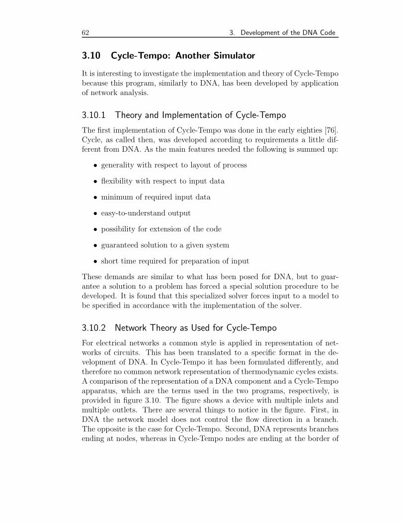
62 3. Development of the DNA Code
3.10 Cycle-Tempo: Another Simulator
It is interesting to investigate the implementation and theory of Cycle-Tempobecause this program, similarly to DNA, has been developed by applicationof network analysis.
3.10.1 Theory and Implementation of Cycle-Tempo
The first implementation of Cycle-Tempo was done in the early eighties [76].Cycle, as called then, was developed according to requirements a little dif-ferent from DNA. As the main features needed the following is summed up:
• generality with respect to layout of process
• flexibility with respect to input data
• minimum of required input data
• easy-to-understand output
• possibility for extension of the code
• guaranteed solution to a given system
• short time required for preparation of input
These demands are similar to what has been posed for DNA, but to guar-antee a solution to a problem has forced a special solution procedure to bedeveloped. It is found that this specialized solver forces input to a model tobe specified in accordance with the implementation of the solver.
3.10.2 Network Theory as Used for Cycle-Tempo
For electrical networks a common style is applied in representation of net-works of circuits. This has been translated to a specific format in the de-velopment of DNA. In Cycle-Tempo it has been formulated differently, andtherefore no common network representation of thermodynamic cycles exists.A comparison of the representation of a DNA component and a Cycle-Tempoapparatus, which are the terms used in the two programs, respectively, isprovided in figure 3.10. The figure shows a device with multiple inlets andmultiple outlets. There are several things to notice in the figure. First, inDNA the network model does not control the flow direction in a branch.The opposite is the case for Cycle-Tempo. Second, DNA represents branchesending at nodes, whereas in Cycle-Tempo nodes are ending at the border of
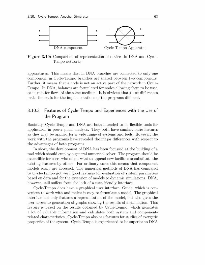
3.10. Cycle-Tempo: Another Simulator 63
DNA component Cycle-Tempo Apparatus
Figure 3.10: Comparison of representation of devices in DNA and Cycle-Tempo networks
apparatuses. This means that in DNA branches are connected to only onecomponent, in Cycle-Tempo branches are shared between two components.Further, it means that a node is not an active part of the network in Cycle-Tempo. In DNA, balances are formulated for nodes allowing them to be usedas mixers for flows of the same medium. It is obvious that these differencesmake the basis for the implementations of the programs different.
3.10.3 Features of Cycle-Tempo and Experiences with the Use ofthe Program
Basically, Cycle-Tempo and DNA are both intended to be flexible tools forapplication in power plant analysis. They both have similar, basic featuresas they may be applied for a wide range of systems and fuels. However, thework with the programs have revealed the major differences with respect tothe advantages of both programs.
In short, the development of DNA has been focussed at the building of atool which should employ a general numerical solver. The program should beextendible for users who might want to append new facilities or substitute theexisting features by others. For ordinary users this means that componentmodels easily are accessed. The numerical methods of DNA has comparedto Cycle-Tempo got very good features for evaluation of system parametersbased on data and for the extension of models to dynamic simulations. DNA,however, still suffers from the lack of a user-friendly interface.
Cycle-Tempo does have a graphical user interface, Guide, which is con-venient to work with and makes it easy to formulate a model. The graphicalinterface not only features a representation of the model, but also gives theuser access to generation of graphs showing the results of a simulation. Thisfeature is based on the results obtained by Cycle-Tempo, which generatesa lot of valuable information and calculates both system and component-related characteristics. Cycle-Tempo also has features for studies of exergeticproperties of the system. Cycle-Tempo is experienced to be superior to DNA
64 3. Development of the DNA Code
with respect to optimization in design of systems. With respect to numer-ical methods Cycle-Tempo employs a specially tailored solver, which dividesthe system of equations into constitutive relations and balance equations.The balance equations are solved in an outer loop, whereas the constitutiverelations are formulated explicitly, and are solved in each iteration in thebalances. Cycle-Tempo gives higher priority to the pressure variables, whichin principle have to be calculated before other quantities.
As a user of Cycle-Tempo, it has been experienced that the program doesnot possess features for an extensive examination of the model. This meansthat a model may have too many quantities specified, and make the systemof equations overdetermined, without giving an error as feedback to the user.The program is a little dubious about which specifications will be overruled.An underdetermined system, however, will always be identified correctly.
3.11 Evaluation of DNA
DNA is only one among many simulation programs available. The programwas developed for two main reasons. First, it is of importance for a universitydepartment working in the field of simulation, to have knowledge about theprocess of building simulators. Second, it is the intention with the develop-ment of DNA to ‘fill a hole’ in the scope of available programs. Lorentzen[72] did research to determine if an existing program was well suited for thebroad purposes stated by the PREFUR framework, and found that nonehad all the wanted features. This conclusion was limited to a few programsand an extension of it, based on work with other programs and on availableliterature, seems to be in place.
A comparison of software including one’s own development may tend tobe rather subjective, because knowledge of one’s own code naturally is muchdeeper than of other codes. The evaluation below mainly is a comparisonof features of different programs. The assessment is based on personal ex-perience from work with Cycle-Tempo [66, 103] and with EES [65] and onliterature presenting programs [4, 10, 29, 36, 37, 54, 69, 97, 110]. The belowlistings of the features of particular program is of course subject to changes,due to ongoing developments.
3.11.1 Approach to Modelling
Many programs are developed to calculate either static or dynamic systems.This means that different programs have to be applied in order to design asystem and to calculate its operating characteristics, respectively. Though
3.11. Evaluation of DNA 65
the application of two different programs allow a user to select the best one foreach task, it does require the user to know both programs well and formulatethe same model in two different environments, which may not be equivalent.Thus, the possibility of using the same program for both applications seemsattractive.
Steady-state-only programs are for instance Cycle-Tempo, DIMAP [69],ESMS [10] and different commercial programs (Aspen+, GateCycle)[54]. Fordynamic simulations only the program of Dymek [29], SpeedUp [54] andMMS [110] are available.
A few program has access to both static and dynamic simulations. In ad-dition to DNA, CAMEL [37], EES [65], Hysys [54] and general mathematicalsoftware as Matlab, Maple may be applied.
The programs Hysys [54], Aspen+, Prosim, GateCycle, Spence and GT-Pro/Master [4] all have features for optimization of a system. SpeedUp isapplicable in optimization of dynamic processes.
3.11.2 Approach to System Specification
The specification of a system model needs to be easy for the user. This ismost conveniently done, if the model may be created by use of componentmodels. This is the approach of most specialized energy system simulatorsand flowsheeting software, e.g., Aspen+, Hysys, GateCycle, Prosim, Cycle-Tempo, DIMAP, Camel, ESMS and DNA. On the other hand, it makesthe use of equation-based, general tools as Matlab and Maple unappealing,also because these programs lack routines for calculation of thermophysicalproperties. This may, however, be overcome by formulation of procedures inthe programs.
The EES program is equation-oriented but it has been programmed withapplication to thermal systems as aim, and therefore does have features forproperties of many substances. This makes the program very relevant forsmaller models.
3.11.3 Approach to Numerical Solution
Most programs use a sequential solver which may be of different nature, per-haps including a combined sequential-simultaneous solver. The system maybe solved as independent equations one by one [36], or as in Cycle-Tempo,where the component equations features its own solver or are formulated ex-plicitly, whereas the balance equations are solved simultaneously. Commer-cial programs as Aspen+, GateCycle, and GT-Pro/Master all have sequential
66 3. Development of the DNA Code
methods. The equation-based programs as EES, Matlab, Maple have sim-ultaneous solvers available. The program DIMAP employs a simultaneoussolver with sparse matrix techniques, but the system of equations is dividedin a special way into different sets including equations for different kinds ofvariables.
It is unquestionable that a standard, implicit numerical solver with re-spect to generality, flexibility and efficiency has the best properties, due towell-known numerical properties and extendibility. However, the applicationof specialized solvers may be advantageous if it is decided that the good fea-tures of standard solvers may be overruled by requiring less flexibility andgenerality of the solver and thereby by the simulation program.
3.11.4 Judgement of the Relevance of DNA
In his summary Lorentzen concludes that “ . . . DNA is a unique, fast andflexible simulation tool . . . ”. Due to the demanding task to set up evena simple model, because of its text interface, DNA may for unexperiencedusers seem difficult to work with and not at all fast and flexible.
From the work with DNA and other programs and from the summary offeatures of simulation programs, it is my opinion, however, that the state-ment of Lorentzen is correct. DNA does have unique features according to thetabular representation of the model, which provides a possibility of extensiveanalysis of the consistency of the model, and according to the carefully selec-ted numerical methods for both algebraic and differential equation systems.DNA is fast due to the simultaneous equation solver utilizing sparse matrixmethods. DNA is flexible because it allows simulation of almost any energysystem, and it allows users to implement new components in an easy way.
4. DEVELOPMENT OF COMPONENTMODELS
Using DNA in simulations is only possible with the desired component modelsavailable. The component library of DNA is a set of FORTRAN routinesbuilt from a template. The template is described in detail in appendix A.The library of components has been updated to make use of the new facilitiesincluding general specification of media, and variable number of branches andsubdivisions. The updated component library is outlined in appendix D. Theset of sample models which has been provided in [72] has been rewritten byextensive use of the new component models.
4.1 Assessment of Existing Models
The library of existing models has been updated making use of the newfeatures added to the code. In addition, some components have had a majorupdate as described below.
4.1.1 Extraction Turbine
In models of steam plants an extraction turbine is essential. Previously, suchturbines have been modelled as a number of serially connected turbines withintermediate splitters modelling the extractions to preheaters. This methodmade it necessary to write large input files with up to, say, 10 turbine models.
Based on the new feature making it possible to write component modelswith a user-specified number of branches, it has been possible to implementa turbine model which allows the user to choose an appropriate number ofextractions from one single model.
In the implemented model the extraction pressures are determined outsidethe model. The enthalpy of steam in the extraction points is calculated byassuming that the extraction follows a straight line in an h–s-diagram.
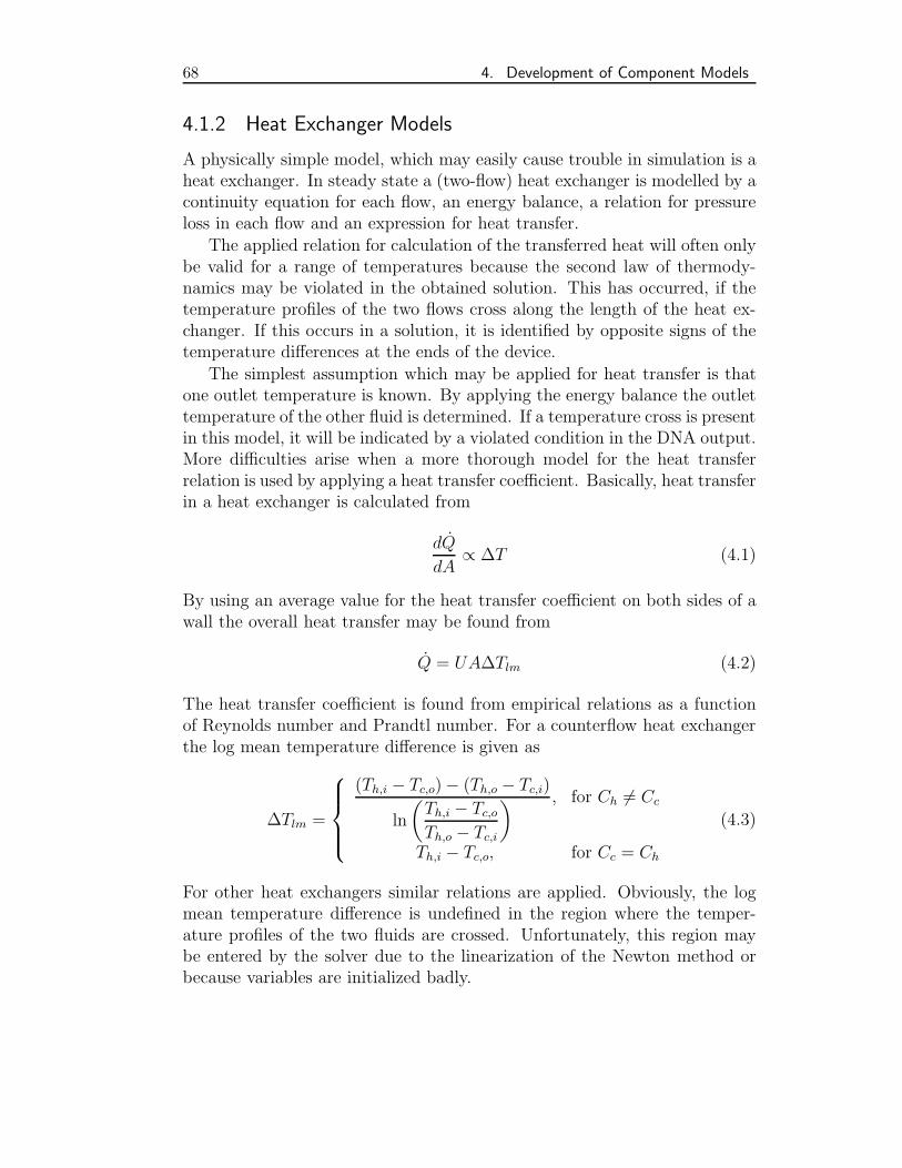
68 4. Development of Component Models
4.1.2 Heat Exchanger Models
A physically simple model, which may easily cause trouble in simulation is aheat exchanger. In steady state a (two-flow) heat exchanger is modelled by acontinuity equation for each flow, an energy balance, a relation for pressureloss in each flow and an expression for heat transfer.
The applied relation for calculation of the transferred heat will often onlybe valid for a range of temperatures because the second law of thermody-namics may be violated in the obtained solution. This has occurred, if thetemperature profiles of the two flows cross along the length of the heat ex-changer. If this occurs in a solution, it is identified by opposite signs of thetemperature differences at the ends of the device.
The simplest assumption which may be applied for heat transfer is thatone outlet temperature is known. By applying the energy balance the outlettemperature of the other fluid is determined. If a temperature cross is presentin this model, it will be indicated by a violated condition in the DNA output.More difficulties arise when a more thorough model for the heat transferrelation is used by applying a heat transfer coefficient. Basically, heat transferin a heat exchanger is calculated from
dQ
dA∝ ∆T (4.1)
By using an average value for the heat transfer coefficient on both sides of awall the overall heat transfer may be found from
Q = UA∆Tlm (4.2)
The heat transfer coefficient is found from empirical relations as a functionof Reynolds number and Prandtl number. For a counterflow heat exchangerthe log mean temperature difference is given as
∆Tlm =
(Th,i − Tc,o)− (Th,o − Tc,i)
ln
(Th,i − Tc,oTh,o − Tc,i
) , for Ch = Cc
Th,i − Tc,o, for Cc = Ch
(4.3)
For other heat exchangers similar relations are applied. Obviously, the logmean temperature difference is undefined in the region where the temper-ature profiles of the two fluids are crossed. Unfortunately, this region maybe entered by the solver due to the linearization of the Newton method orbecause variables are initialized badly.
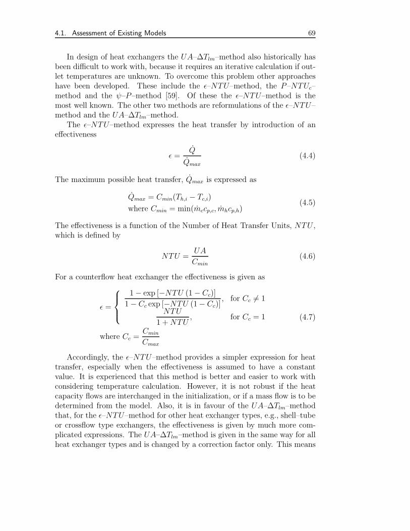
4.1. Assessment of Existing Models 69
In design of heat exchangers the UA–∆Tlm–method also historically hasbeen difficult to work with, because it requires an iterative calculation if out-let temperatures are unknown. To overcome this problem other approacheshave been developed. These include the ε–NTU–method, the P–NTUc–method and the ψ–P–method [59]. Of these the ε–NTU–method is themost well known. The other two methods are reformulations of the ε–NTU–method and the UA–∆Tlm–method.
The ε–NTU–method expresses the heat transfer by introduction of aneffectiveness
ε =Q
Qmax
(4.4)
The maximum possible heat transfer, Qmax is expressed as
Qmax = Cmin(Th,i − Tc,i)
where Cmin = min(mccp,c, mhcp,h)(4.5)
The effectiveness is a function of the Number of Heat Transfer Units, NTU ,which is defined by
NTU =UA
Cmin
(4.6)
For a counterflow heat exchanger the effectiveness is given as
ε =
1− exp [−NTU (1− Cc)]
1− Cc exp [−NTU (1− Cc)], for Cc = 1
NTU
1 +NTU, for Cc = 1
where Cc =Cmin
Cmax
(4.7)
Accordingly, the ε–NTU–method provides a simpler expression for heattransfer, especially when the effectiveness is assumed to have a constantvalue. It is experienced that this method is better and easier to work withconsidering temperature calculation. However, it is not robust if the heatcapacity flows are interchanged in the initialization, or if a mass flow is to bedetermined from the model. Also, it is in favour of the UA–∆Tlm–methodthat, for the ε–NTU–method for other heat exchanger types, e.g., shell–tubeor crossflow type exchangers, the effectiveness is given by much more com-plicated expressions. The UA–∆Tlm–method is given in the same way for allheat exchanger types and is changed by a correction factor only. This means
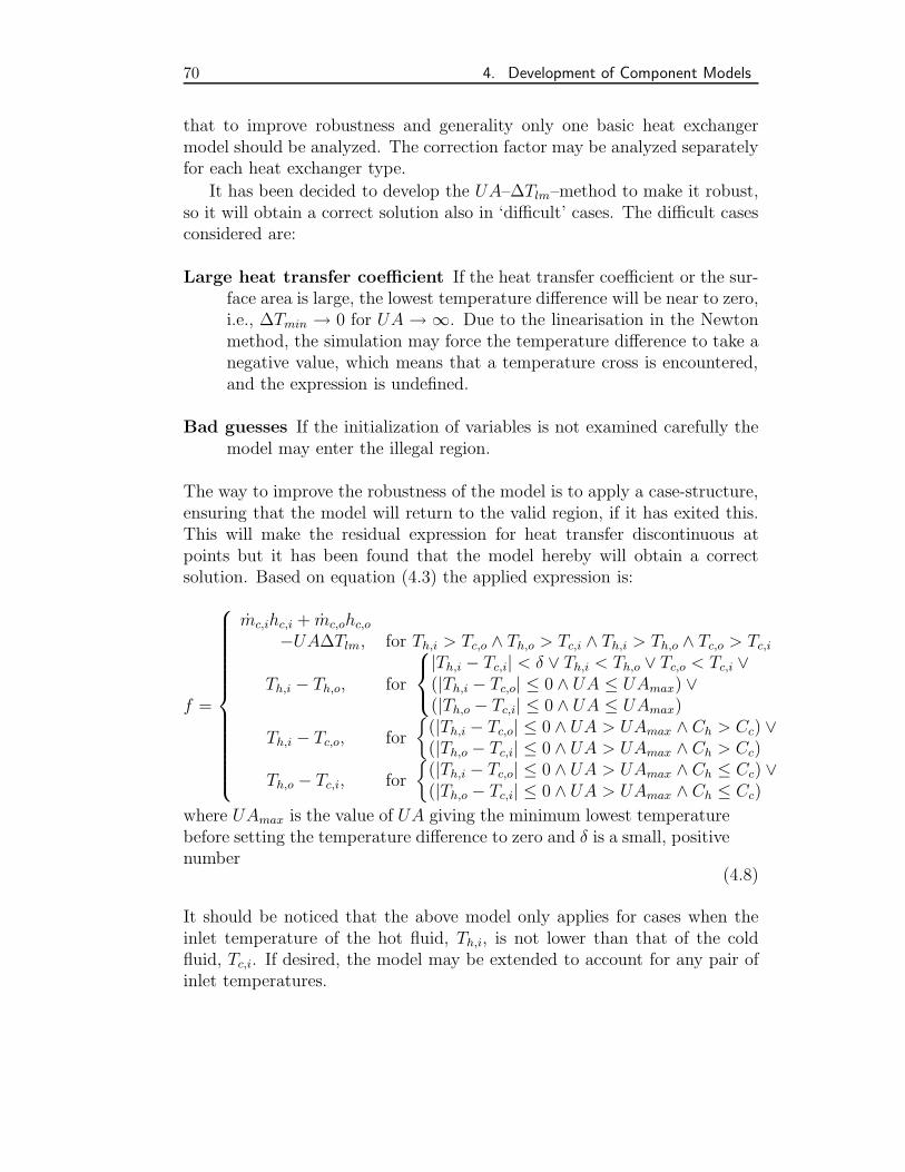
70 4. Development of Component Models
that to improve robustness and generality only one basic heat exchangermodel should be analyzed. The correction factor may be analyzed separatelyfor each heat exchanger type.
It has been decided to develop the UA–∆Tlm–method to make it robust,so it will obtain a correct solution also in ‘difficult’ cases. The difficult casesconsidered are:
Large heat transfer coefficient If the heat transfer coefficient or the sur-face area is large, the lowest temperature difference will be near to zero,i.e., ∆Tmin → 0 for UA → ∞. Due to the linearisation in the Newtonmethod, the simulation may force the temperature difference to take anegative value, which means that a temperature cross is encountered,and the expression is undefined.
Bad guesses If the initialization of variables is not examined carefully themodel may enter the illegal region.
The way to improve the robustness of the model is to apply a case-structure,ensuring that the model will return to the valid region, if it has exited this.This will make the residual expression for heat transfer discontinuous atpoints but it has been found that the model hereby will obtain a correctsolution. Based on equation (4.3) the applied expression is:
f =
mc,ihc,i + mc,ohc,o−UA∆Tlm, for Th,i > Tc,o ∧ Th,o > Tc,i ∧ Th,i > Th,o ∧ Tc,o > Tc,i
Th,i − Th,o, for
|Th,i − Tc,i| < δ ∨ Th,i < Th,o ∨ Tc,o < Tc,i ∨(|Th,i − Tc,o| ≤ 0 ∧ UA ≤ UAmax) ∨(|Th,o − Tc,i| ≤ 0 ∧ UA ≤ UAmax)
Th,i − Tc,o, for
(|Th,i − Tc,o| ≤ 0 ∧ UA > UAmax ∧ Ch > Cc) ∨(|Th,o − Tc,i| ≤ 0 ∧ UA > UAmax ∧ Ch > Cc)
Th,o − Tc,i, for
(|Th,i − Tc,o| ≤ 0 ∧ UA > UAmax ∧ Ch ≤ Cc) ∨(|Th,o − Tc,i| ≤ 0 ∧ UA > UAmax ∧ Ch ≤ Cc)
where UAmax is the value of UA giving the minimum lowest temperaturebefore setting the temperature difference to zero and δ is a small, positivenumber
(4.8)
It should be noticed that the above model only applies for cases when theinlet temperature of the hot fluid, Th,i, is not lower than that of the coldfluid, Tc,i. If desired, the model may be extended to account for any pair ofinlet temperatures.
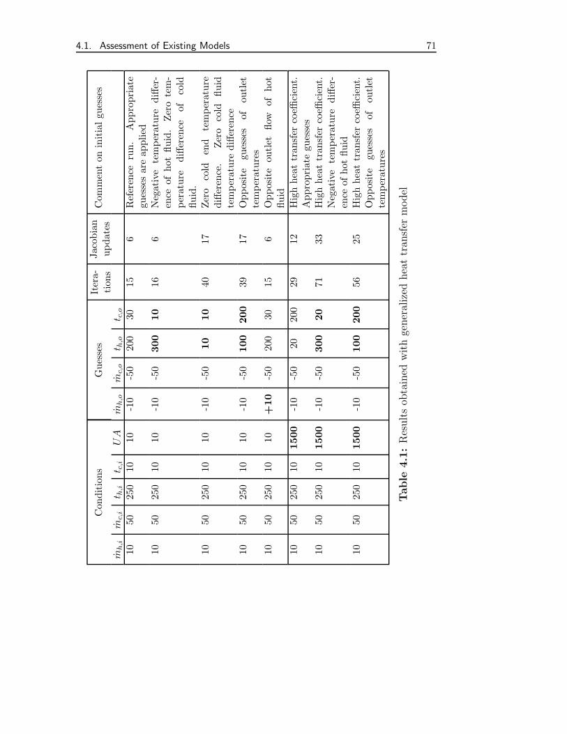
4.1. Assessment of Existing Models 71
Conditions
Guesses
Itera-
tions
Jacobian
updates
Com
menton
initialguesses
mh,i
mc,i
t h,i
t c,i
UA
mh,o
mc,o
t h,o
t c,o
1050
250
1010
-10
-50
200
3015
6Reference
run.
Appropriate
guessesareapplied
1050
250
1010
-10
-50
300
1016
6Negativetemperature
differ-
ence
ofhotfluid.Zerotem-
perature
differenceof
cold
fluid.
1050
250
1010
-10
-50
1010
4017
Zerocold
end
temperature
difference.
Zerocold
fluid
temperaturedifference
1050
250
1010
-10
-50
100
200
3917
Oppositeguessesof
outlet
temperatures
1050
250
1010
+10
-50
200
3015
6Oppositeoutlet
flow
ofhot
fluid
1050
250
1015
00-10
-50
20200
2912
Highheattransfercoefficient.
Appropriateguesses
1050
250
1015
00-10
-50
300
2071
33Highheattransfercoefficient.
Negativetemperature
differ-
enceofhotfluid
1050
250
1015
00-10
-50
100
200
5625
Highheattransfercoefficient.
Oppositeguessesof
outlet
temperatures
Table
4.1
:Resultsobtained
withgeneralized
heattransfer
model
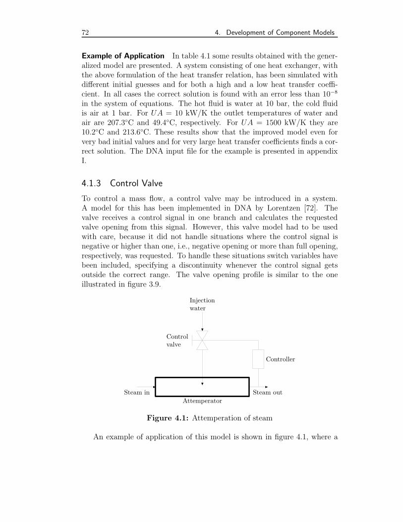
72 4. Development of Component Models
Example of Application In table 4.1 some results obtained with the gener-alized model are presented. A system consisting of one heat exchanger, withthe above formulation of the heat transfer relation, has been simulated withdifferent initial guesses and for both a high and a low heat transfer coeffi-cient. In all cases the correct solution is found with an error less than 10−8
in the system of equations. The hot fluid is water at 10 bar, the cold fluidis air at 1 bar. For UA = 10 kW/K the outlet temperatures of water andair are 207.3C and 49.4C, respectively. For UA = 1500 kW/K they are10.2C and 213.6C. These results show that the improved model even forvery bad initial values and for very large heat transfer coefficients finds a cor-rect solution. The DNA input file for the example is presented in appendixI.
4.1.3 Control Valve
To control a mass flow, a control valve may be introduced in a system.A model for this has been implemented in DNA by Lorentzen [72]. Thevalve receives a control signal in one branch and calculates the requestedvalve opening from this signal. However, this valve model had to be usedwith care, because it did not handle situations where the control signal isnegative or higher than one, i.e., negative opening or more than full opening,respectively, was requested. To handle these situations switch variables havebeen included, specifying a discontinuity whenever the control signal getsoutside the correct range. The valve opening profile is similar to the oneillustrated in figure 3.9.
AttemperatorSteam in Steam out
Controlvalve
Injectionwater
Controller
Figure 4.1: Attemperation of steam
An example of application of this model is shown in figure 4.1, where a
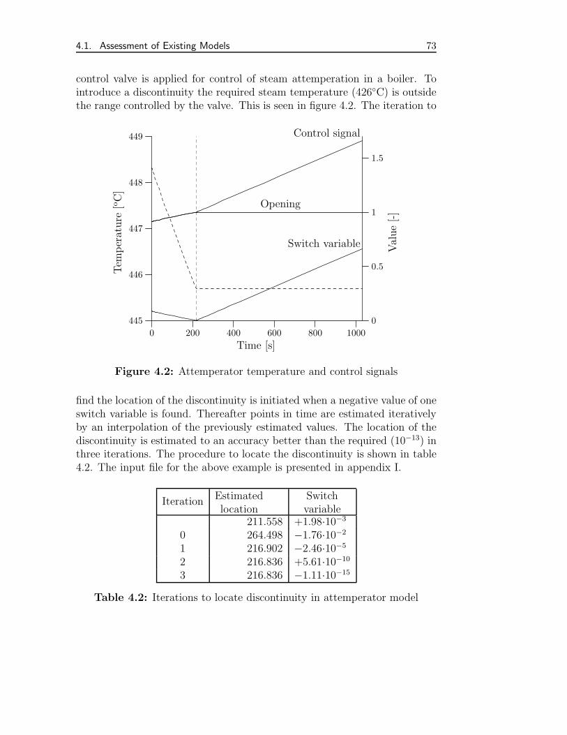
4.1. Assessment of Existing Models 73
control valve is applied for control of steam attemperation in a boiler. Tointroduce a discontinuity the required steam temperature (426C) is outsidethe range controlled by the valve. This is seen in figure 4.2. The iteration to
445
446
447
448
449
Opening
Control signal
Switch variable
0 200 400 600 800 10000
0.5
1
1.5
Time [s]
Value[-]
Tem
perature
[oC]
Figure 4.2: Attemperator temperature and control signals
find the location of the discontinuity is initiated when a negative value of oneswitch variable is found. Thereafter points in time are estimated iterativelyby an interpolation of the previously estimated values. The location of thediscontinuity is estimated to an accuracy better than the required (10−13) inthree iterations. The procedure to locate the discontinuity is shown in table4.2. The input file for the above example is presented in appendix I.
IterationEstimatedlocation
Switchvariable
211.558 +1.98·10−3
0 264.498 −1.76·10−2
1 216.902 −2.46·10−5
2 216.836 +5.61·10−10
3 216.836 −1.11·10−15
Table 4.2: Iterations to locate discontinuity in attemperator model
74 4. Development of Component Models
4.2 Boiler Model Specific Development
4.2.1 Furnace Model
The furnace model should resemble the heat transfer from the combustionproducts through the waterwall and to water flowing through the pipes. Heattransfer inside the furnace is governed by radiation and convection, throughthe wall material by conduction and between pipe and water by convection.Each mode of heat transfer is to be analyzed to formulate a model for thefurnace operation. The pressure loss occurring from friction, gravity andacceleration of the fluid also has to be accounted for. Hadvig [43] outlinesa way to model simultaneous heat transfer in different modes, expressing anoverall heat transfer coefficient, Utot, and make use of the formulation:
Q = UtotA∆Tlm (4.9)
The overall heat transfer coefficient is found from [11]
Utot =1
rA· 1
1
αgro+
1
λwlnrori
+1
αstri
where rA is the radius at which the transfer area is calculated
(4.10)
The three terms in the denominator are the thermal resistance of flue gas,wall and steam, respectively. Relations for expression of the heat transfercoefficients of fluids have to be established.
The pipes are only heated on the side facing the furnace. This has tobe accounted for in the transferring surface area. Due to convection in thepipe material, the transferring area will not be the same for each term ofthe overall heat transfer. On the outside of the tubes, the transferring areawill be about half of the pipe surface. On the inside the convective heattransfer coefficient will be dependent on the non-uniformity of the transferprofile [107]. The non-uniformity of the surface area may be correlated bya sinusoidal curve from which the average heat transfer coefficient is foundto be in the range of 80–100% of what it would be for a circumferentially,symmetrically heated pipe. The overall heat transfer coefficient based on thetotal inside surface area may be expressed as:
Utot,i =1
ri· 1
1
0.5αgro+
1
0.75λwlnrori
+1
0.9αstri
(4.11)
In this the profile for conduction is assumed to be more non-symmetricalthan it is for inside convection.
4.2. Boiler Model Specific Development 75
Radiative Heat Transfer in Furnace The furnace of the boiler has in sev-eral system studies been modelled by a fully lumped model, by introductionof the Konakow Number, Ko [23, 29]. For this study a fully lumped modelhas been assumed to be inappropriate, because it cannot provide any inform-ation about the temperature distribution in the furnace. Instead, a divisionof the furnace has been done by assuming profiles of, e.g., heat transfer andcombustion product concentrations, to be symmetrical about the verticalcenter axis of the furnace. The furnace then is divided into slices of equalheight. All stages have sides made up by the furnace waterwall and only thetop and bottom stages need separate model formulations because they donot have both transparent top and bottom boundary.
The heat balance for a surface, i, in an enclosure will be [43]:
Qi = Ai (Hi −Bi) (4.12)
Qi is the net incoming radiation to surface i with the total surface area Ai. Hi
and Bi are the irradiation and the emittance from the surface, respectively.The emittance from a surface is:
Bi = εiσT4w,i + ρiHi (4.13)
The sum of emissivity and reflectivity is for non-transmittant surfaces equalto unity.
In [44] the irradiation to a surface is formulated as the sum of the radiationfrom the gas and any surface in the enclosure. This sum may be expressedas:
Hi =
N∑j=1
FijτjiBj + εgiσT4g (4.14)
Fij is the view factor from surface i to j. It expresses the amount of thehemisphere above surface i occupied by surface j. τji is the transmissivity ofthe gas for radiation from surface j to surface i. Its value is τji = 1− αji.
A few relations for view factors may be of importance to notice. Thesummation rule:
N∑i=1
Fij = 1 (4.15)
The reciprocity relation:
AiFij = AjFji (4.16)
76 4. Development of Component Models
Their importance will be exploited in the derivations below.
The modelling approach for the above is based on lumping assumptionsfor the enclosure. This is also the case for the furnace which, however, maybe subdivided into smaller lumps or compartments. The interface betweentwo parts of a furnace is regarded as a fully transmittant border, which allowsany irradiation to be transported into the neighbouring compartment. Tworelations express the behaviour of a transmittant boundary, i, for radiativetransfer:
Bi = Hi−1 (4.17)
Bi−1 = Hi (4.18)
This is naturally only valid for fully transmittant surfaces. Surfaces bothtransmitting, absorbing and reflecting radiation may be introduced in thismodelling approach, if needed in future studies.
Comparison to Other Radiation Analysis Methods The approach is com-parable to the zone method originating from the work of Hottel and Sarofimand described in [89]. The zone method is the most commonly applied inradiation analysis. In the zone method the enclosure surface is divided intosmaller parts, zones. The amount τjiAiFij is called the direct exchange areafor radiation from surface i to j. It is defined between all surfaces in anenclosure and directly incorporates the extinction of radiation due to gas ab-sorbtivity. In the same manner direct exchange areas between gas volumesand surfaces are defined. The zone method is ordinarily applicable to greygas models only, but this problem may be overcome.
The method applied in the present study involving transparent walls willend up in the same methodology, as the extinction of radiation beams will begoverned by the transmissivity of the gas in any volume passed by radiationfrom one surface to another. A model for an industrial furnace based on avery similar approach has been developed by Herapath and Peskett [46].
Determination of View Factors In addition to the above relations the viewfactors are determined. In one compartment, the wall is assumed to have aconstant temperature and it may accordingly be seen as one surface, w. Thetop, t, and bottom, b boundaries are the two other surfaces in the enclosure.
4.2. Boiler Model Specific Development 77
An expression for view factors between two parallel surfaces is given in [43]:
Ft,bπXY
2=Y
√1 +X2 arctan
(Y√
1 +X2
)+X
√1 + Y 2 arctan
(X√
1 + Y 2
)+
ln
(√(1 +X2)(1 + Y 2)
1 +X2 + Y 2
)− Y arctanY −X arctanX
(4.19)
where X and Y are ratios between the length of the surface sides and thedistance between the surfaces. For square surfaces which are common infurnaces the expression simplifies to:
Ft,bπX2
2= 2X
√1 +X2 arctan
(X√
1 +X2
)+ ln
(1 +X2
√1 + 2X2
)− 2X arctanX
(4.20)
Due to symmetry
Fb,t = Ft,b (4.21)
Fb,w = Ft,w (4.22)
Fw,b = Fw,t (4.23)
and due to geometry
Fb,b = Ft,t = 0 (4.24)
From equation (4.15) and symmetry the following relations can be obtained:
Ft,w = Fb,w = 1− Fb,t (4.25)
Fw,w = 1− 2Fw,t (4.26)
And finally, by application of the reciprocity rule equation (4.16) is foundthat:
AwFw,t = AtFt,w (4.27)
In the hopper, the view factor is obtained, similarly, by application ofequation (4.19) and Yamamutis rule [43], which makes it possible to calculateview factor between non-parallel surfaces.
For each compartment in a furnace a non-linear equation system of threeheat balances for top, bottom and wall is formed. Solving this system a heattransfer coefficient similar to the one for convection may be defined by:
Q = αradAw(Tg − Tw) (4.28)
78 4. Development of Component Models
where the wall temperature is at the outside of the pipes. This temperatureis also applied in the calculation of emitted radiation from the pipes. Forthe actual model including the partitioning, determination of a heat transfercoefficient for radiation is inconvenient because it would have to be expressedfrom the above described non-linear equation system. Instead, it is easier todetermine the heat flow and equal it to the heat transferred through wall andto water.
Convective Heat Transfer Inside Tubes Heat transfer inside tubes is forsingle-phase fluids a relatively well-described topic. An equation which maybe applied over a large range of flow characteristics is [53]:
Nu =α
λD=
f
8(Re− 1000)Pr
1 + 12.7
√f
8(Pr2/3 − 1)
(4.29)
For smooth tubes the friction factor may be found from
f = (0.79 lnRe− 1.64)−2 (4.30)
The Nusselt number for superheated steam and for liquid water may becalculated according to equation (4.29). Also water at supercritical pressurehas been calculated by this equation. Fluid properties should be taken asthe mean of inlet and outlet values for pressure and temperature. Specificvolume and viscosity should be evaluated according to the mean pressureand the mean temperature to have consistent values.
At supercritical pressure in the vicinity of the critical point, the fluid isstill single-phase, but the thermal properties are highly dependent on tem-perature [23, 91] and equation (4.29) cannot be applied as is. An approachbased on a selective averaging of thermal conductivity at five temperatureshas been presented in [42].
In boiling two-phase flows the heat transfer will be highly influenced bythe present flow regime [23]. For each region relations for calculation of heattransfer may be applied. In other studies, for example [91] somewhat moresimple and perhaps more imprecise relations are used.
In the developed model, the single-phase relation has been assumed to bea sufficiently good approximation also for two-phase flow at low load.
Pressure Loss in Tubes For flow inside boiler tubes pressure loss will becaused by friction, gravity and changes in specific volume.
∆p = ∆pf +∆pg +∆pa (4.31)
4.2. Boiler Model Specific Development 79
The frictional pressure loss is
∆pf = 4fl
d
ρw2
2(4.32)
For turbulent flow, i.e., Re > 2300, the friction factor is determined by [53]
f = (0.79 lnRe + 1.64)−2 (4.33)
Gravitational pressure loss can be found as
∆pg = ρg∆H (4.34)
Pressure loss due to change in flow velocity is
∆pa = ρiw2i − ρow
2o (4.35)
In the model additional pressure loss due to other resistances in the pipingis added as equivalent lengths.
4.2.2 Superheater Model
The superheater model is only valid for crossflow tube bundle heat ex-changers. The hot gasses flow through a tube bundle inside which steamis superheated. Depending on pitch and temperature level the heat transferon the gas side of a superheater will be both convective and radiative. Themodel has been applied to superheaters with rectangular pitch. The profileof these is shown in figure 4.3, which also illustrates some parameters usedin the analysis of tube bundle heat exchangers. All pipes have the samediameter, d. The center distance between two pipes is SL and ST paralleland perpendicular to the flow direction, respectively. The number of tubesin both directions is much higher than shown in the figure. The rectangle,VF , shown by dashed lines encloses a part of the superheater which has beenanalysed to determine radiative view factors. Due to the assumptions themost appropriate formulation of the heat transfer in the bundle is given as
Q = FcfUA∆Tlm,
where U =1
rA
11
ro (αg + αr)+
1
λwlnrori
+1
αsri
(4.36)
The heat transfer coefficient is found as a combined coefficient for radiativeand convective transfer on the gas side. The correction factor for cross flow tocounterflow models, Fcf , is in [62] only available for single-pass tube bundles.As the superheater sections are constructed as multi-pass bundles, it has beenassumed that these may be modelled as multiple single-pass exchangers.
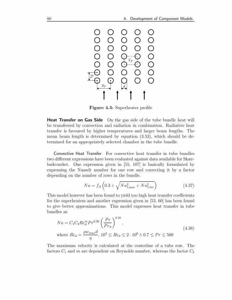
80 4. Development of Component Models
ST
SL
d
VF
Figure 4.3: Superheater profile
Heat Transfer on Gas Side On the gas side of the tube bundle heat willbe transferred by convection and radiation in combination. Radiative heattransfer is favoured by higher temperatures and larger beam lengths. Themean beam length is determined by equation (3.53), which should be de-termined for an appropriately selected chamber in the tube bundle.
Convective Heat Transfer For convective heat transfer in tube bundlestwo different expressions have been evaluated against data available for Skær-bækværket. One expression given in [55, 107] is basically formulated byexpressing the Nusselt number for one row and correcting it by a factordepending on the number of rows in the bundle.
Nu = fA
(0.3 +
√Nu2
1,lam +Nu21,tur
)(4.37)
This model however has been found to yield too high heat transfer coefficientsfor the superheaters and another expression given in [53, 60] has been foundto give better approximations. This model expresses heat transfer in tubebundles as
Nu = C1C2Remd Pr
0.36
(Pr
PrS
)0.25
,
where Red =ρwmaxd
η, 103 ≤ Red ≤ 2 · 106 ∧ 0.7 ≤ Pr ≤ 500
(4.38)
The maximum velocity is calculated at the centerline of a tube row. Thefactors C1 and m are dependent on Reynolds number, whereas the factor C2
4.2. Boiler Model Specific Development 81
is less than one for tube bundles with less than twenty rows.
Cross flow correction factor An expression for the correction factor Fcf forcross flow heat exchangers is given in [62]. These algebraic expressions havebeen preferred to the polynomial approximations in [107]. It has been foundthat the derivations in [62] for cross flow heat exchangers is not calculatedcorrectly due to confusion in the definition of the temperature group (r) fordifferent types of heat exchangers. (r) is defined as
(r) =∆T
Th,i − Tc,i(4.39)
and therefore may be expressed as
(r) =mccp,cUA
· tc,o − tc,iTh,i − Tc,i
(4.40)
Defining the quantities
S =tc,o − tc,ith,i − tc,i
(4.41)
R =th,i − th,otc,o − tc,i
(4.42)
For counterflow exchangers (r) can be expressed as
(r) =S(R− 1)
ln
(1− S
1− RS
) (4.43)
The superheaters are assumed to work as cross flow heat exchangers withthe hot fluid, flue gas, mixed and the cold fluid, steam, unmixed. The tem-perature group is for this type found to be [62]
(r)cf =S
ln
(1 +
ln (1− RS)
R
) (4.44)
The correction factor to apply for the superheater models may then be foundas
Fcf =(r)cfr
=
ln
(1− S
1− RS
)(1− R) ln
(1 +
ln (1−RS)
R
) (4.45)
82 4. Development of Component Models
As given here the correction factor is not applicable for any applied set oftemperatures, and it has to be extended for improvement of the robustness.The value of Fcf may not be outside the interval [0; 1], because such val-ues are physically impossible, but may if present allow the numerical solverto obtain a mathematically correct solution outside the physically correctinterval. Some limits for which the expression is undefined, are
limS→0
Fcf = 1 (4.46)
limR→0
Fcf = 1 (4.47)
limR→∞
Fcf = 1 (4.48)
limR→1
Fcf =S
(S − 1) ln(1 + ln(1− S))(4.49)
limS→ 1−e−R
R
Fcf = 0 (4.50)
To be applicable for any set of temperature values the correction factor canbe formulated as:
Fcf =
1, for
th,i = tc,i ∨ S = 0∨(th,i ≤ th,o ∧ th,o ≥ th,i)
0, for
(th,i ≤ th,o ∧ tc,i ≥ tc,o)∨(R = 1 ∧ S > 1− e−1)∨RS > 1− e−R
S
(S − 1) ln(1 + ln(1− S)), for R = 1 ∧ S ≤ 1− e−1
ln
(1− S
1−RS
)(1− R) ln
(1 +
ln (1− RS)
R
) , else
(4.51)
Fin efficiency Some of the lower temperature superheaters are equippedwith transverse fins to increase heat recovery. The fin efficiency for transversefins of constant width is given as [62]:
ηf =2
ub − ue· I1 (ub)− β1K1 (ub)
I0 (ub)− β1K0 (ub)(4.52)
where
β1 =I1(ue)
K1(ue)(4.53)
4.2. Boiler Model Specific Development 83
ub = rb
√αf
kyb(4.54)
ue = re
√αf
kyb= ub
rerb
(4.55)
The Modified Bessel functions may be approximated by polynomials [1].
Radiation Analysis To determine radiative transfer in the tube bundle,an approach similar to the one applied for the furnace has been made. Thetotal volume of the bundle is divided into rectangular enclosures as indicatedin figure 4.3 by VF . Each of the enclosures is bounded by the four quartercircles of the pipes and by transmitting boundaries. It is assumed that thepipes have the same temperature, and that the gas has the same temperaturein each of the enclosures. Hereby the pipes may be seen as one surface, 1,and the transmitting boundaries as one other, 2. Irradiation to the total pipesurface in an enclosure is found as:
H1 = (1− αg)(F11B1 + F21B2) + εgσT4g (4.56)
The pipes emit heat according to:
B1 = εwσT4w + ρwH1 (4.57)
The transmitting boundaries will transmit the same heat at both sides, dueto the assumption of constant gas temperature:
B2 = (1− αg)(F12B1 + F22B2) + εgσT4g (4.58)
Solving equations 4.56–4.58 the total heat transfer by radiation from gas towalls can be found from
Q1 = A1(H1 −B1) (4.59)
As indicated in figure 4.3 the tube bundle profile seems to be built aspaths separated by each vertical row of tubes. To determine view factorsand beam length, it is assumed that the tube length is very large comparedto each chamber. If the chamber is assumed to be rectangular, the meanbeam length may then be expressed as:
L = 3.5A
P= 3.5
NTSTSL
2(NTSL + ST )(4.60)
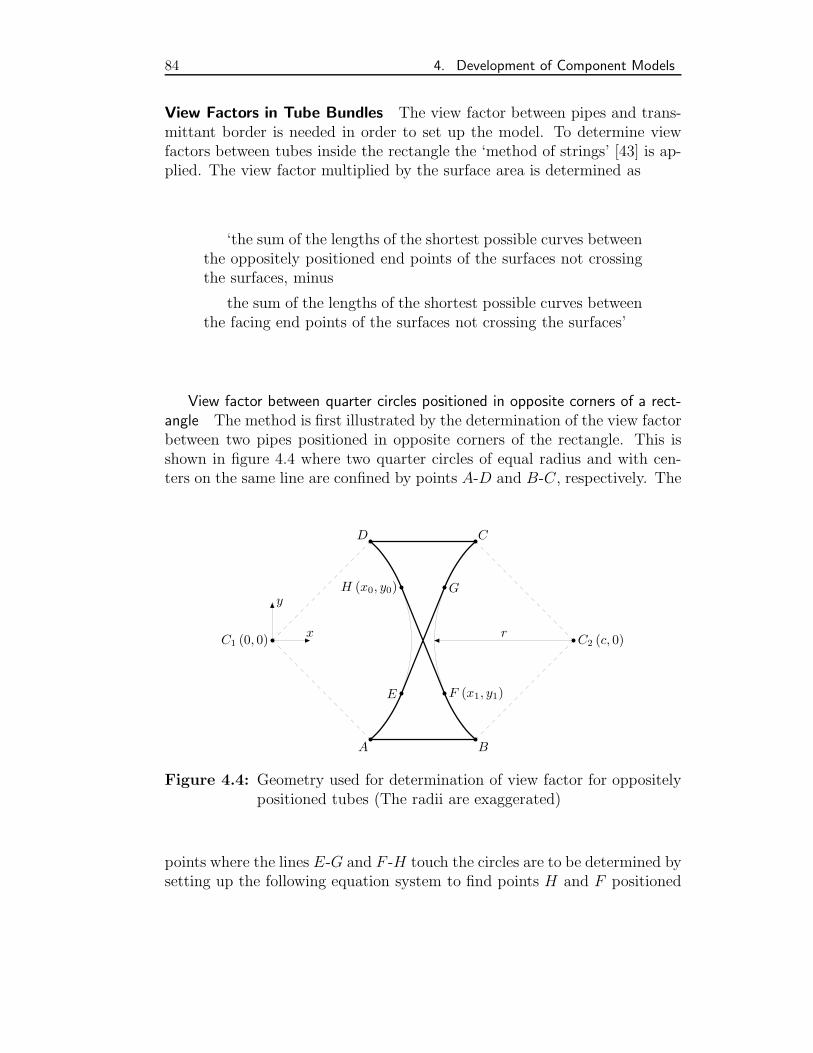
84 4. Development of Component Models
View Factors in Tube Bundles The view factor between pipes and trans-mittant border is needed in order to set up the model. To determine viewfactors between tubes inside the rectangle the ‘method of strings’ [43] is ap-plied. The view factor multiplied by the surface area is determined as
‘the sum of the lengths of the shortest possible curves betweenthe oppositely positioned end points of the surfaces not crossingthe surfaces, minus
the sum of the lengths of the shortest possible curves betweenthe facing end points of the surfaces not crossing the surfaces’
View factor between quarter circles positioned in opposite corners of a rect-angle The method is first illustrated by the determination of the view factorbetween two pipes positioned in opposite corners of the rectangle. This isshown in figure 4.4 where two quarter circles of equal radius and with cen-ters on the same line are confined by points A-D and B-C, respectively. The
C1 (0, 0) C2 (c, 0)
A B
CD
E F (x1, y1)
GH (x0, y0)
rx
y
Figure 4.4: Geometry used for determination of view factor for oppositelypositioned tubes (The radii are exaggerated)
points where the lines E-G and F -H touch the circles are to be determined bysetting up the following equation system to find points H and F positioned
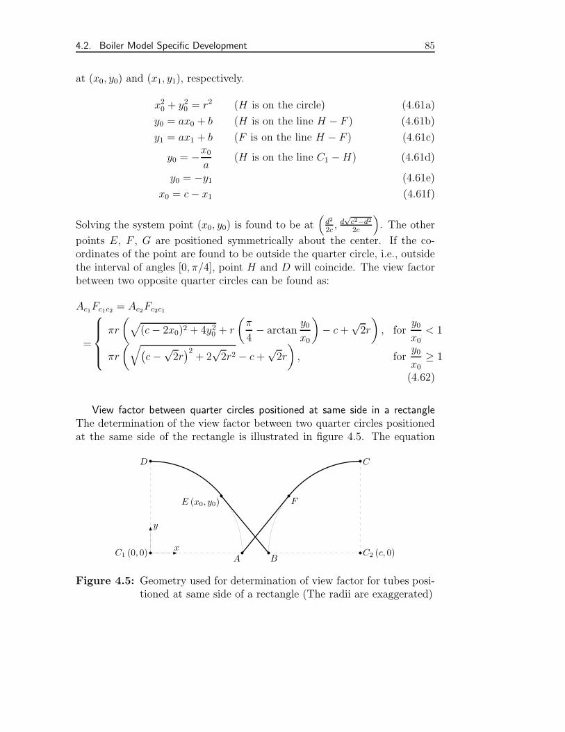
4.2. Boiler Model Specific Development 85
at (x0, y0) and (x1, y1), respectively.
x20 + y2
0 = r2 (H is on the circle) (4.61a)
y0 = ax0 + b (H is on the line H − F ) (4.61b)
y1 = ax1 + b (F is on the line H − F ) (4.61c)
y0 = −x0
a(H is on the line C1 −H) (4.61d)
y0 = −y1 (4.61e)
x0 = c− x1 (4.61f)
Solving the system point (x0, y0) is found to be at(d2
2c, d
√c2−d2
2c
). The other
points E, F , G are positioned symmetrically about the center. If the co-ordinates of the point are found to be outside the quarter circle, i.e., outsidethe interval of angles [0, π/4], point H and D will coincide. The view factorbetween two opposite quarter circles can be found as:
Ac1Fc1c2 = Ac2Fc2c1
=
πr
(√(c− 2x0)2 + 4y2
0 + r
(π
4− arctan
y0
x0
)− c+
√2r
), for
y0
x0
< 1
πr
(√(c−√
2r)2+ 2
√2r2 − c+
√2r
), for
y0
x0
≥ 1
(4.62)
View factor between quarter circles positioned at same side in a rectangleThe determination of the view factor between two quarter circles positionedat the same side of the rectangle is illustrated in figure 4.5. The equation
C1 (0, 0) C2 (c, 0)A B
CD
E (x0, y0) F
x
y
Figure 4.5: Geometry used for determination of view factor for tubes posi-tioned at same side of a rectangle (The radii are exaggerated)
86 4. Development of Component Models
system applied to determine the position of point E at (x0, y0) is given as
x20 + y2
0 = r2 (E is on the circle) (4.63a)
y0 = ax0 + b (E is on the line E −B) (4.63b)
0 = a(c− r) + b (B is on the line E −B) (4.63c)
y0 = −x0
a(E is on the line C1 −E) (4.63d)
The coordinates of point (x0, y0) turns out as (r2(c−r)−1, r(c−r)−1
√c(c− 2r) ).
The view factor may be determined from
Ac1Fc1c2 = Ac2Fc2c1
= πr
(√(c− r − x0)2 + y2
0 + r
(π
2− arctan
(y0
x0
))− c+ r
)(4.64)
The view factor from pipes to pipes, F11, is determined by relations given forsubdivided surfaces. For a surface, j, divided into n components, the viewfactor for radiation from surface i to j is:
Fij =n∑
k=1
Fik (4.65)
and by introduction of the reciprocity relation, the view factor for radiationfrom surface j to surface i is:
AjFji =
n∑k=1
AkFki (4.66)
If one quarter circle of the rectangle VF in figure 4.3 is seen as a surface, Ci,the view factor from this quarter circle to the total pipe surface, 1, inside VFis given by equation (4.65):
FCi1 =
4∑k=1
FC1Ck(4.67)
Due to symmetry FC11 = FC21 = FC31 = FC41. As the surface areas of thequarter circles also are equal, equation (4.66) can be applied to obtain:
A1F11 = 4AC1F11 =4∑
k=1
ACkFCk1 = 4AC1FC11
⇔F11 = FC11
(4.68)
4.3. BIGCC Model Specific Development 87
The other view factors in the volume can be found from the sum rule andthe reciprocity relation:
F11 + F12 = F21 + F22 = 1 (4.69)
A1F12 = A2F21 (4.70)
Flue Gas Pressure Loss in Tube Bundles Pressure loss for flow across banksof tubes may be found from
∆p = ∆pf +∆pg (4.71)
The frictional pressure loss is in [107] given as:
∆pf = ξNRρwmax
2(4.72)
The friction factor is evaluated as
ξ = ξlam + ξtur =flamRe
+ftur
Re0.1b/a
where flam = flam(a, b), ftur = ftur(a, b), a =ST
d, b =
SL
d
(4.73)
Each friction factor term is corrected for variable physical properties along
the flow direction by a factor of the form(µw
µ
)r, where r is a constant for
the turbulent regime and is a function of geometry, Reynolds number andthe number of rows in the laminar regime.
4.3 BIGCC Model Specific Development
To extend the possibilities for primarily simulation of gasification installa-tions and combustion, the inclusion of solid fuels as possible flow media hasbeen important. In a simulation of a biomass IGCC-plant, this feature isneeded for all processes upstream of the fuel entry to the gasifier. Of import-ant models developed for this application, a dryer and a gasifier is describedbelow.
4.3.1 Solid Fuel Dryer
The solid fuel dryer is a drum in which warm flue gas is in direct contact withthe fuel. Hereby the fuel is heated and moisture evaporates. Regarding afuel dryer from a modelling viewpoint, the properties to be handled includes
88 4. Development of Component Models
the calculation of outlet composition of dried fuel, calorific value and specificheat of the fuel and the amount of evaporated water.
The model is not very detailed, and this description mainly shows how amodel including solid flows is formulated.
The desired amount of moisture in the outlet fuel is given on mass basisto the model as a parameter. Thereby the composition of outlet fuel can befound from the composition of inlet fuel.
With the obtained composition, the specific heat and heating value ofthe fuel can be found by assumption of a simple average between fuel andmoisture.
Dryer Modelling with Cycle-Tempo The dryer is one of the models appliedin the study of a biomass gasification plant (see chapter 6). Accordingly, amodel for it also is needed in the Cycle-Tempo model. When working withCycle-Tempo, users are not encouraged to include new component models,so a work-round had to be found. Another difficulty is that Cycle-Tempocannot change the properties of a solid fuel flowing through a component,so the change in heating value and specific heat during drying cannot bemodelled.
A model, which is equivalent to the dryer model, therefore has been for-mulated by application of the existing models. The model consists of threecomponents, serially connected in the gas flow. The first model is a heat ex-changer, which evaporates the excessive moisture, which is entering as waterat atmospheric pressure. In the second component, a mixer, the steam ismixed with the flue gas. In the last component, another heat exchanger, theremaining part of the solid fuel is heated to the temperature present in thedryer.
4.3.2 Gasifier 1
In order to model a gasification a more comprehensive model is needed.A gasifier model has been implemented in DNA by Emsholm [35]. Themodel was formulated to calculate the composition of syngas from a reactionbetween a fuel and steam and/or air as gasifier agents. Due to the limitationsof DNA then the model employed ideal gasses for solid fuels and therebyobtained too high efficiencies, due to the difference between gas and solidfuel heating values. The fuel type added to the gasifier has been changedto a solid fuel, in order to have a more realistic model. The model also hasbeen changed to make it possible to account for ashes in the fuel. The outlet
1 Parts of this section are based on [34]
4.3. BIGCC Model Specific Development 89
ash consists of ash entering with the fuel and the carbon which has not beenconverted in the gasifier.
The model of the gasification process is based on the assumption thatchemical equilibrium is present in the resulting syngas. This is a valid as-sumption for coal gasifiers, but it is somewhat more questionable for bio-mass fuels [14]. However, the assumption of chemical equilibrium of syngasprovides a relatively simple model, though it is based on chemical principles.This approach to modelling of gasification has also been taken in the devel-opment of Cycle-Tempo [103] and DIMAP [3].
Formulation and Implementation of Chemical Equilibrium Model Themost appropriate way to determine the composition of a chemical equilib-rium involving a number of possible compounds is to base the calculationon the fact that at equilibrium the Gibbs’ free energy of the gas will takeits minimum value. The Gibbs Free Energy, G, of a gas, assumed to be amixture of, k, perfect gasses, is given by:
G =
k∑i=1
ni(g0i +RT ln yip
)(4.74)
Each atomic element in the inlet fuel and the gasification media to thegasifier should be balanced with the outlet gas composition. This yields thatthe flow of each atom (C, H, N, S, O, Ar . . . ) has to be conserved. This isfor N elements expressed as:
k∑i=1
ni,inAij =k∑
i=1
ni,outAij , for j = 1, N (4.75)
where Aij is the number of molecules of atom j in component i. The min-imization of Gibbs’ Free Energy is formulated by introducing a LagrangeMultiplier, µ, for each of the N constraints obtained from equation (4.75).After addition of the constraints, the expression to minimize then is:
F = Gout +
N∑j=1
µj
(k∑
i=1
(ni,out − ni,in)Aij
)(4.76)
The partial derivatives of equation (4.76) with respect to each gas componentni,out are
∂F
∂ni,out=
g0i,out
RT+ ln(yi,outp) +
k∑j=1
µjAij for i = 1, k (4.77)
90 4. Development of Component Models
At the minimum each of these is zero.
The introduction of Lagrange multipliers provides a method to formulatethe minimization problem as a system of non-linear equations, which is solvediteratively.
Sequential and Simultaneous Implementation of the Chemical Equilib-rium Model The model of Emsholm has been implemented in the DNAcode and works with the program. The implementation features its owninternal iteration to solve the subsystem of equations derived by extractingthe above equations 4.76 and 4.77 from the system. This approach, whichhas also been made in [3], may at first glance seem advantageous, becausethe highly non-linear minimization problem is solved independently. How-ever, it turns the solution method into a combined sequential-simultaneousone, which does not have the well-known properties of the overall solver.Furthermore, the program already features a well-suited solver for non-linearequations, and to improve efficiency this should be applied. Using the overallsolver also retains the desired modularity of the code. A comparison of theefficiency of the two different solution modes is provided below.
Sequential Solution Mode A sequential solution of the gasification modelis in this case carried out by applying a model which divides the solution intotwo parts. The first part is the overall equation system which includes theconservation laws. The Gibbs’ Energy minimization, however, is separatedfrom the system and is done by the component submodel procedure for eachiteration. This implementation is straightforward, because it involves onlyapplication of the above presented equations, and it does not involve theinclusion of the non-linear partial derivatives in the global iteration loop.The cost, on the other hand, is that the equations for the minimization haveto be solved iteratively in the inner loop for each outer loop iteration.
Simultaneous Solution Mode For simultaneous solver implementationsthe equation system has to be changed slightly to avoid singularities. Thisproblem has to do with the application of the mass balance and the atombalances, equation (4.75), which will introduce a linear dependency in theequation system. This problem is easily recognized when the mass balanceis seen as a sum of molar fractions:
m = ninMin
k∑i=1
yi,in = noutMout
k∑i=1
yi,out (4.78)
4.3. BIGCC Model Specific Development 91
where n is the total molar flow and M is the mean molar weight of the gasmixture. Substituting with the atom balances, it is realized that equation(4.78) is superfluous.
However, an additional equation is needed to make the system consistent.In an energy system simulation it is common to always fulfill the continuityequation, and thereby require one of the atom balances to be replaced. Theequation which has to be introduced is a summation of molar fractions of thesyngas:
k∑i=1
yi,out = 1 (4.79)
It is interesting that this substitution is not needed in the proposed sequentialapproach because the solution procedure is split into two parts, each of thembeing underdetermined equation systems in a global view.
Case Study of Biomass Gasification As a case study gasification of 4.0 kg/sof wood at 92C with the elemental analysis 5.20%H, 36.12%O, 0.47%N,42.48%C, 0.05%S, 15% water and 0.68% ashes on weight basis is considered.The gasification media is 4.5 kg/s atmospheric air at 100C and the chem-ical equilibrium of the resulting syngas is on volume basis 21.4%H2, 32.6%N2,24.5%CO, 8.9%CO2, 8.7%H2O, 3.4%CH4 and less than 1% of Ar, H2S andNH3 at 687
oC and 28.5 bar. The equilibrium is calculated at 860oC.The gasifier has been simulated in both sequential and simultaneous mode
with DNA with the same results. For comparison the model has also beensimulated with Cycle-Tempo [103]. This program calculates the same com-position of the syngas, but the temperature is about 100C higher. This hasto do with differences in default assumptions of the fuel properties.
In Cycle-Tempo unconverted carbon may be present in the resulting gas.This is in this case specified not to be allowed in DNA. For low gasifica-tion temperatures where the reactivity is lower, this results in different gascompositions obtained with the two programs.
The assumption of chemical equilibrium does in this case not result in aprecise calculation of the syngas composition [32]. To illustrate the differencesbetween the two solution modes this example serves well enough, however.
Comparison of Simulation Time Simulations of the model in both modeshave been carried out on a 120 MHz Pentium PC with 16 MB of RAM. DNAhas been compiled with the Salford FTN77 compiler using no optimizationfunctionality.
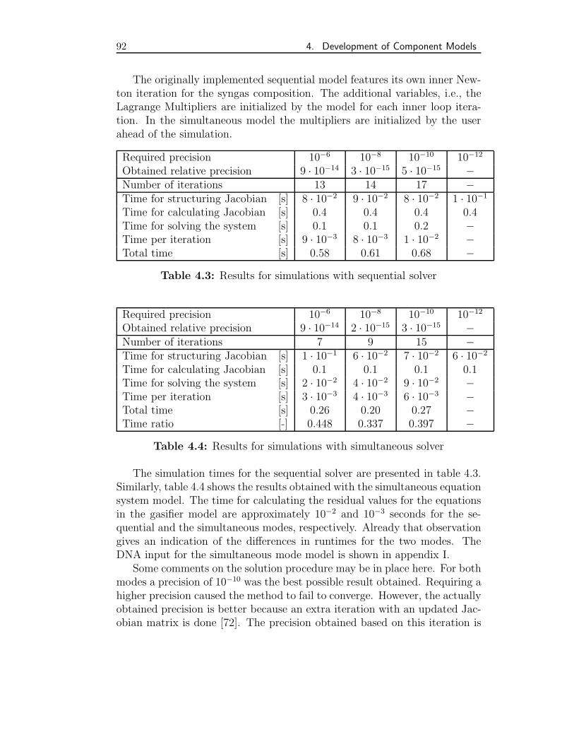
92 4. Development of Component Models
The originally implemented sequential model features its own inner New-ton iteration for the syngas composition. The additional variables, i.e., theLagrange Multipliers are initialized by the model for each inner loop itera-tion. In the simultaneous model the multipliers are initialized by the userahead of the simulation.
Required precision 10−6 10−8 10−10 10−12
Obtained relative precision 9 · 10−14 3 · 10−15 5 · 10−15 −Number of iterations 13 14 17 −Time for structuring Jacobian [s] 8 · 10−2 9 · 10−2 8 · 10−2 1 · 10−1
Time for calculating Jacobian [s] 0.4 0.4 0.4 0.4Time for solving the system [s] 0.1 0.1 0.2 −Time per iteration [s] 9 · 10−3 8 · 10−3 1 · 10−2 −Total time [s] 0.58 0.61 0.68 −
Table 4.3: Results for simulations with sequential solver
Required precision 10−6 10−8 10−10 10−12
Obtained relative precision 9 · 10−14 2 · 10−15 3 · 10−15 −Number of iterations 7 9 15 −Time for structuring Jacobian [s] 1 · 10−1 6 · 10−2 7 · 10−2 6 · 10−2
Time for calculating Jacobian [s] 0.1 0.1 0.1 0.1Time for solving the system [s] 2 · 10−2 4 · 10−2 9 · 10−2 −Time per iteration [s] 3 · 10−3 4 · 10−3 6 · 10−3 −Total time [s] 0.26 0.20 0.27 −Time ratio [-] 0.448 0.337 0.397 −
Table 4.4: Results for simulations with simultaneous solver
The simulation times for the sequential solver are presented in table 4.3.Similarly, table 4.4 shows the results obtained with the simultaneous equationsystem model. The time for calculating the residual values for the equationsin the gasifier model are approximately 10−2 and 10−3 seconds for the se-quential and the simultaneous modes, respectively. Already that observationgives an indication of the differences in runtimes for the two modes. TheDNA input for the simultaneous mode model is shown in appendix I.
Some comments on the solution procedure may be in place here. For bothmodes a precision of 10−10 was the best possible result obtained. Requiring ahigher precision caused the method to fail to converge. However, the actuallyobtained precision is better because an extra iteration with an updated Jac-obian matrix is done [72]. The precision obtained based on this iteration is
4.3. BIGCC Model Specific Development 93
indeed near to the machine precision of approximately 10−16. Even the solu-tions with the lowest required precision end up having a maximum relativeerror of approximately 10−13 for both modes. This indicates the quadraticconvergence of the Newton method and also that one may not need to requirea very high precision in the iterations to get an accurate solution.
The simultaneous solver requires fewer iterations than the sequential,meaning that measuring the efficiency by the convergence speed also favoursthe simultaneous implementation.
The big difference between the methods is seen in the numerical evalu-ation of the Jacobian matrix and in the solution times for the iterative pro-cedure which both require equation evaluations. Rather large overall timesavings of up to 64% are found.

94 4. Development of Component Models
5. SIMULATION OF BOILERDYNAMICS
5.1 Description of the Boiler of Skærbækværket Unit 3
The studied boiler is the one of unit 3 of the Skærbækværket. The boiler is ofthe once-through type and is operated at supercritical steam parameters atfull load. The boiler produces ??? MW from live steam at 335 bar / 610C.The boiler is designed for a process with double reheat of the steam.
A schematic figure of the boiler indicating its main installations is shownin figure 5.1. The figure shows the positioning of the superheater sectionsand the number of passes in each. Each superheater/reheater is built bymore of these stages. The air preheater is positioned above the economizer,but is not shown as no data have been available for it.
5.2 Model of the Boiler
5.2.1 Methodology Applied for Modelling of the Plant
The developed model of the boiler is based on the DNA models outlined inchapter 4. Each component model has been calibrated to model the operationof the plant at full load. The data available for calibration of the model areequipment layout and operating data for 100% load at different locations inthe boiler of Nordjyllandsværket unit 3 [63]. This boiler is constructively thesame as the boiler of Skærbækværket unit 3, but it is fuelled by coal insteadof natural gas. The influences of this difference on the model are describedbelow (section 5.2.2). The implementation of the model as DNA input isoutlined in appendix G.
The component models have been connected to form a full model of theboiler. In order to simulate the plant at different loads, it is necessary toinclude models of the other parts of the plant. A summary of the additionalcomponents in the model are given in section 5.2.2.
Data for the operation of Skærbækværket unit 3 under a change of load
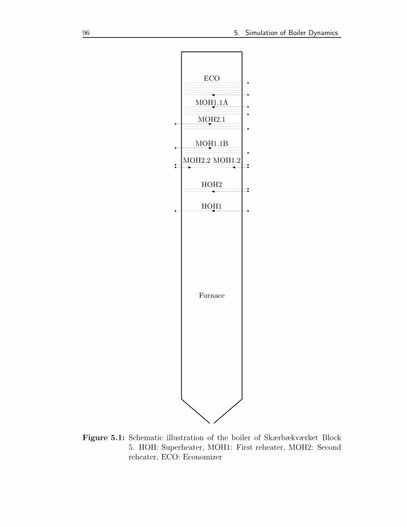
96 5. Simulation of Boiler Dynamics
HOH1
HOH2
MOH1.2MOH2.2
MOH1.1B
MOH2.1
MOH1.1A
ECO
Furnace
Figure 5.1: Schematic illustration of the boiler of Skærbækværket Block5. HOH: Superheater, MOH1: First reheater, MOH2: Secondreheater, ECO: Economizer
5.2. Model of the Boiler 97
have been supplied by Elsamprojekt [78]. The data provide values of pressure,temperature and flow measured with 5 seconds interval during a load changefrom 39% to 33%.
Data for the operation of both plants are proprietary and are only shownas relative values in the results below.
The main objective of this study has been to show that DNA is applicablein simulation of dynamics of complex energy systems. The developed modeldoes have limitations, due to limited knowledge of the plant and simplifiedcomponent models.
5.2.2 Simplification and Assumptions
In order to implement the model in DNA and to keep the amount of timeused for this part of the study within the time available, some simplificationsand assumptions have been necessary to apply to the model. Below the mostimportant of these are described.
Combustion The combustion process is in the model assumed to take placein a separate component, which delivers the combustion products to the fur-nace. The physical meaning of this assumption is that combustion of allfuel happens instantaneously, which is of course incorrect. In the model theresult of this assumption is that a separation of the furnace into more com-partments is only possible if the flue gasses are added to the compartmentsaccording to some appropriate distribution function. Otherwise, a much toolarge driving temperature difference between gas and water wall would bepresent in the compartment where gas enters.
Adequate distributions of the inlet gas have been found for division of thefurnace into two and three parts, but there is no simple relation which givesthe distribution because it involves both reaction kinetics for the combustionand fluid dynamics of the gas-air mixture inside the furnace. To apply themodel at different loads with an assumed distribution of gas, therefore hasbeen regarded as inappropriate and only a one-compartment furnace com-ponent is applied in the model.
Fuel The model has been calibrated using data for the coal-fired boiler ofNordjyllandsværket and applying the instantaneous combustion model de-scribed above. Due to this, the gasses in the furnace have a little differentthermophysical properties than in the real boiler. A comparison of the prop-erties of the two gas mixtures calculated according to [44, 72, 88] only show
98 5. Simulation of Boiler Dynamics
minor differences considering specific heat, transport properties and radiativeproperties of gas and particles.
Dynamic Modelling In DNA a dynamic model may be applied for anyrelevant quantity. The most important variables are mass and energy contentin a fluid inside a component and energy content of the metal in a component.The developed model only covers the dynamic effects of steel in the majorheat transferring parts of the boiler, i.e., furnace and superheaters. Thedynamic effects of the fluids has been neglected because the energy contentof gas and steam is very limited compared to the steel, even though steamhas a high specific heat compared to steel.
Only in the economizer where water is liquid, the energy content is sig-nificant. However, the temperature of steam in the economizer is nearlyconstant and the dynamic effects are limited.
Three-flow components Due to the limitation in DNA, which only allowsup to two flows to be present in a model, the furnace and superheaters havebeen simplified. The water walls surrounding superheaters are not consideredand the radiation shielding part of the high pressure superheater is consideredto have same surface temperature as the evaporator tubes.
Control System No data for the control system of the plant have beenavailable. This means that control principles of the boiler and transients dueto this have not been possible to model and that some assumptions havebeen necessary. These assumptions may be summarized as follows:
Load control The control of the load of the plant is in the model made bythe mass flow of combustion gases, which follows the desired load.
Sliding pressure The boiler is operated with sliding pressure which meansthat both pressure and mass flow of high pressure steam are propor-tional to the load [23]. Steam pressure is in the model calculated ac-cording to this.
Steam Temperature The temperature of steam to each turbine sectionis controlled by means of attemperation. However, the temperatureof steam leaving each superheater section is not kept constant for allloads [79]. The exact strategy for control of the steam temperatureis complicated and the steam to each turbine section is in the modelassumed to be constant.
5.3. Design-load Steady-state Model 99
Extraction steam The mass flow of steam to the last turbine section maybe modelled as being proportional to the pressure [16], i.e., by a turbineconstant. For turbines not expanding to vacuum more complex applic-ations of Stodola’s ellipse may be applied. However, due to lack of datafor the characteristics of the turbines of the actual plant, it is assumedthat a turbine constant gives a sufficiently good approximation to theoperating characteristics.
Heat Exchange In the evaporator tubes only the relation for convectiveheat exchange for supercritical pressures, i.e., for single-phase flow, isused. For two-phase flows either much simpler and inappropriatelyinaccurate relations [45] or much more complex relations involving de-termination of location of different flow regimes in the evaporator tubes[23] are needed. Inclusion of more complex relations has not been pos-sible within this study.
5.3 Design-load Steady-state Model
Data for operation of the boiler of Nordjyllandsværket at full load have beensupplied by Elsamprojekt [63] and have been used for calibration of themodel.
The objective of the calibration has been to obtain appropriate values forthe parameters of the component models. Most parameters, such as pipe sizesand masses, are specified in the data and have been used. In order to make themodel applicable, knowledge of thermophysical properties of steel are needed.Values for these have been obtained by application of thermodynamic dataof gas and steam in a steady-state model. The properties which have beenrelevant to calculate are, emissivity of the piping and additional pressurelosses originating in equipment which have been neglected in the model,e.g., mixing headers.
The emissivity of the water wall of the furnace has been calculated to be0.8, which is a realistic value. In the superheaters a value of 0.3 for each hasbeen found. This value seems rather low, but it may be explained by someof the assumptions included in the model. The water wall of the superheaterhas been neglected and any heat transfer to it has accordingly been neglected.
5.4 Model of Load Change
Data for a load change of Skærbækværket from 39% to 33% load have beenfound and made available by Elsamprojekt. The data provide measurements
100 5. Simulation of Boiler Dynamics
of flow, temperature and pressure of water/steam at many locations in theboiler and of gas and air flow at 5 seconds interval. The measurements havebeen obtained over more than 5000 seconds operations. For the first morethan 1500 seconds the load of the plant is constantly 39%. Similarly, afterabout 4000 seconds the load change is ended and the load is 33%, constantly.
The simulations run with the model of the plant only models the timeof the load change in order to shorten the simulation time. One problem inthe application of the model has been observed. During the load change theload becomes so low that injection water in the second reheater is no longerrequired. This gives rise to a discontinuity which is included in the model.However, the mass flow is zero, and DNA does not handle this very well. Thesimulations are stopped by the program, when this occurs.
5.4.1 Results for Flow
In figure 5.2 data and results for the flow of gas and steam and the load ofthe plant are compared. As described the flow of gas in the model equals thedesired load. Due to the simple assumptions for the plant control and theneglected dynamics of the mass in the boiler, the small fluctuations in thedata are not seen in the results. The assumptions also require the mass flowof feedwater to follow the load demand. This is seen not to be the case forthe real operation of the plant.
5.4.2 Results for Pressure
In figure 5.3, page 102, results for the pressure of steam are compared to data.A comparison of the graphs shows that the assumption of proportionalitybetween mass flow and pressure is not valid for the low load simulated. Themodel, however, does resemble the trend of the pressure of steam.
5.4.3 Results for Temperature
The temperature of steam in the high pressure part of the boiler is shown infigure 5.4, page 103. It is seen that the assumption of constant temperatureout of the superheater, i.e., perfect control, is not correct. The temperatureis decreasing. However, the model does show the trend, that the temperatureout the two superheaters in the high pressure section approach each otherduring the load change, within the time range covered by the simulation.
In both reheaters the steam temperature is assumed to be constant at allloads. Also here it is seen from the graphs in figure 5.5, page 104 and figure
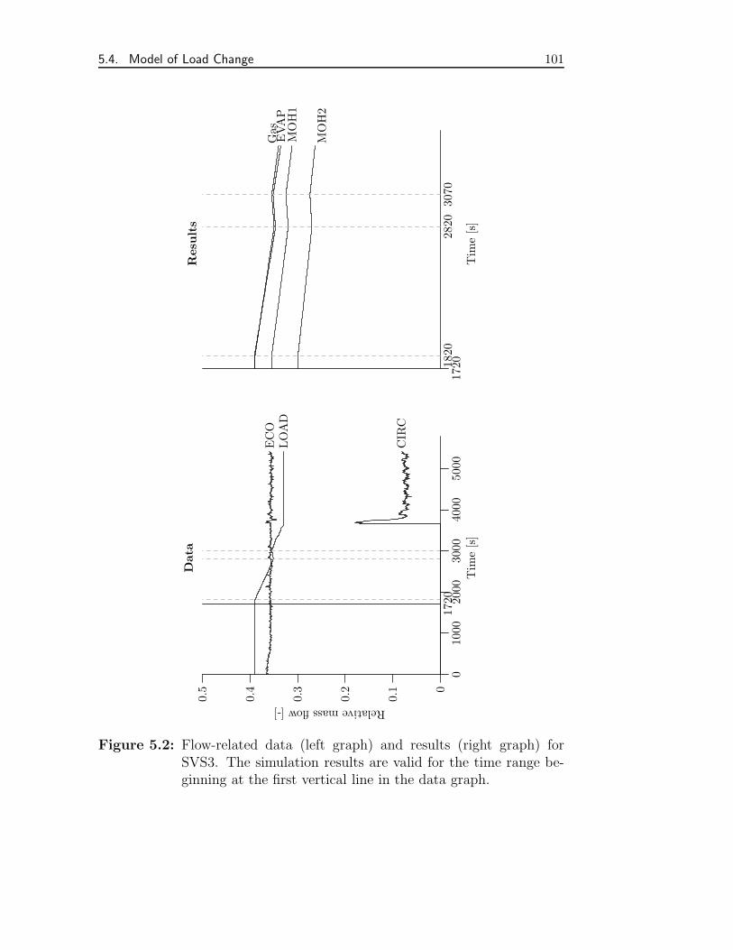
5.4. Model of Load Change 101
LOAD
CIRC
ECO
01000
2000
3000
4000
5000
0
0.1
0.2
0.3
0.4
0.5
1720
Time[s]
Dat
a
Relativemassflow[-]
Gas
EVAP
MOH1
MOH2
17201820
2820
3070
Time[s]
Res
ult
s
Figure 5.2: Flow-related data (left graph) and results (right graph) forSVS3. The simulation results are valid for the time range be-ginning at the first vertical line in the data graph.
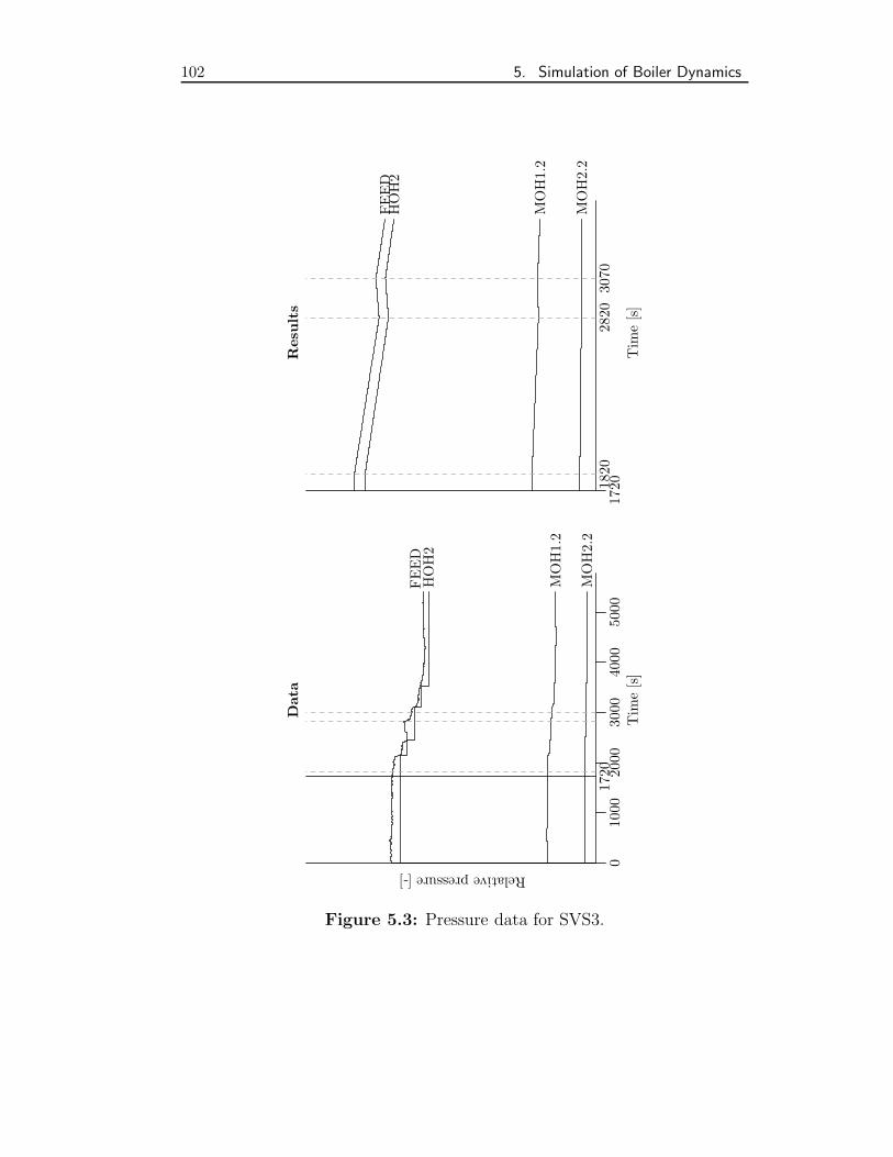
102 5. Simulation of Boiler Dynamics
MOH1.2
MOH2.2
FEED
HOH2
01000
2000
3000
4000
5000
1720
Time[s]
Dat
aRelativepressure[-]
FEED
HOH2
MOH1.2
MOH2.2
17201820
2820
3070
Time[s]
Res
ult
s
Figure 5.3: Pressure data for SVS3.
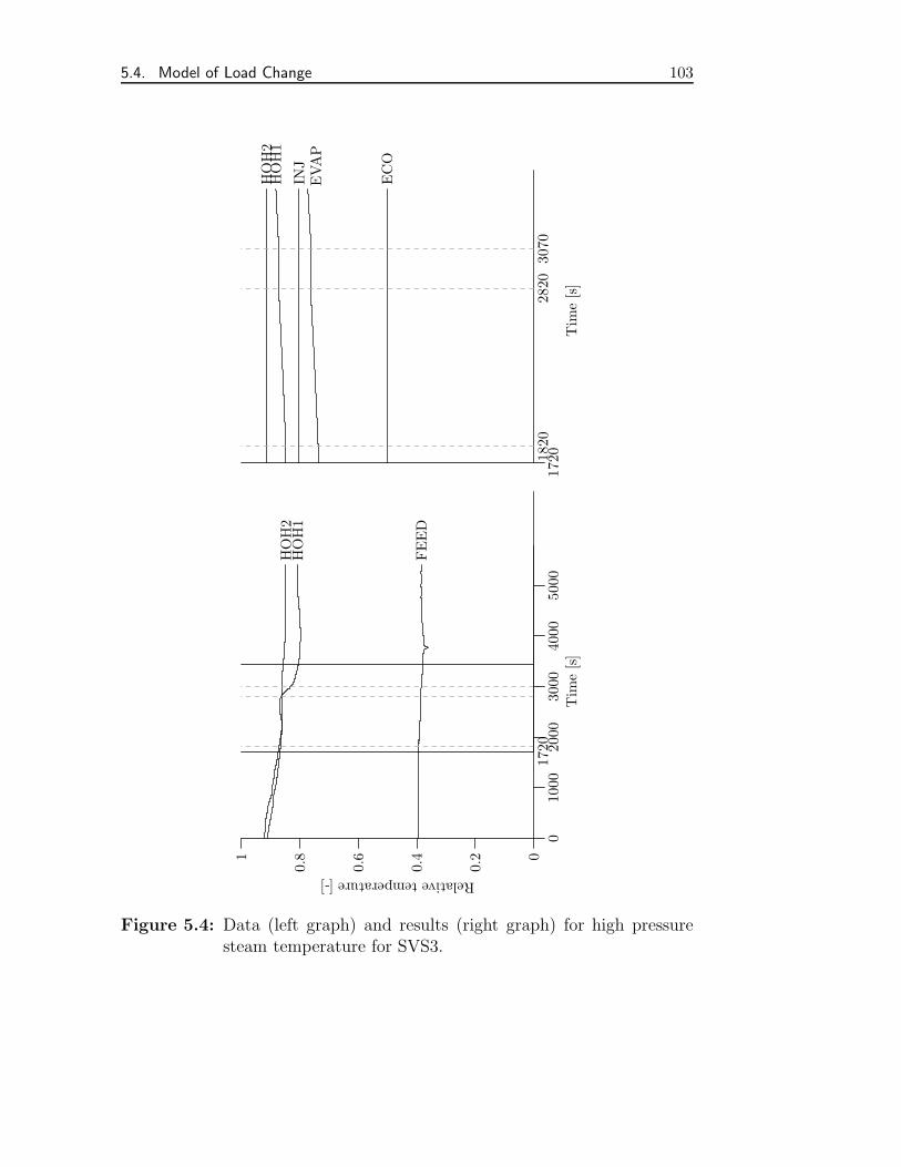
5.4. Model of Load Change 103
FEED
HOH1
HOH2
01000
2000
3000
4000
5000
0
0.2
0.4
0.6
0.81
1720
Time[s]
Relativetemperature[-]
ECO
EVAP
HOH1
INJ
HOH2
17201820
2820
3070
Time[s]
Figure 5.4: Data (left graph) and results (right graph) for high pressuresteam temperature for SVS3.
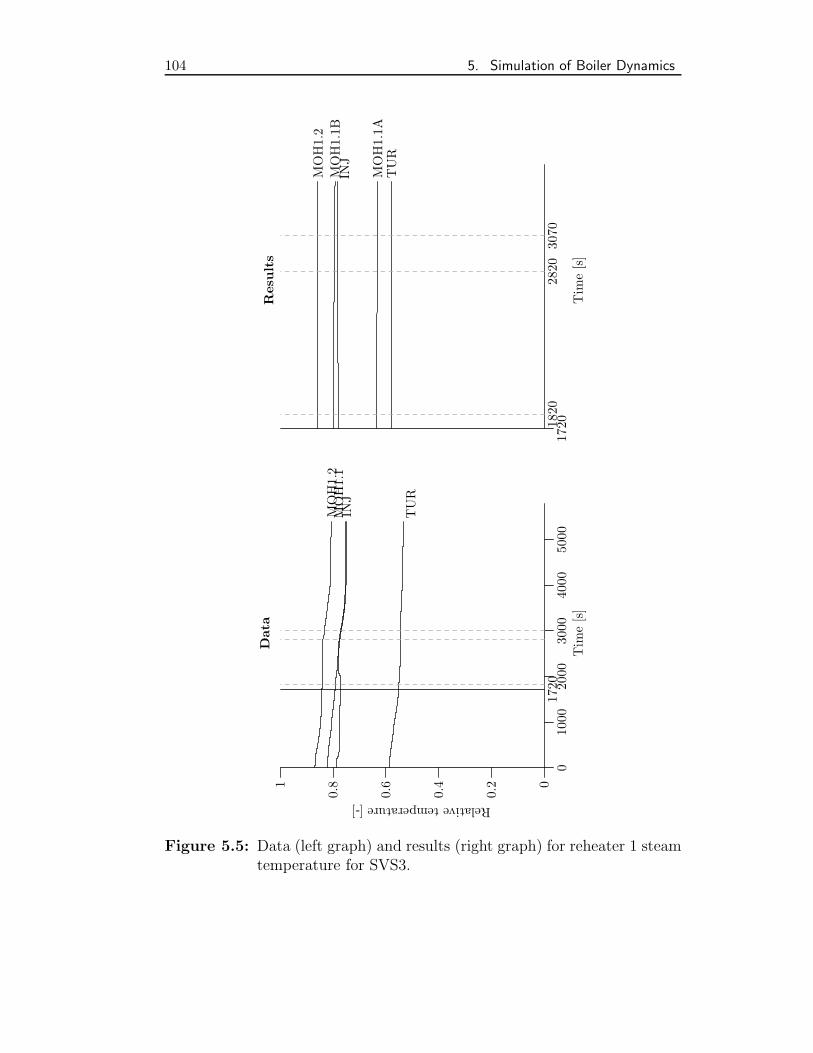
104 5. Simulation of Boiler Dynamics
INJ
MOH1.1
MOH1.2
TUR
01000
2000
3000
4000
5000
0
0.2
0.4
0.6
0.81
1720
Time[s]
Dat
a
Relativetemperature[-]
TUR
MOH1.1A
MOH1.1B
INJ
MOH1.2
17201820
2820
3070
Time[s]
Res
ult
s
Figure 5.5: Data (left graph) and results (right graph) for reheater 1 steamtemperature for SVS3.
5.5. Discussion of Results 105
5.6, page 106 that this is not the case in the operation of the plant. However,some trends of the data are resembled by the simulation.
In figure 5.5 the temperature of steam in the first reheater section isdisplayed. It is seen that the temperature of steam out the two reheaters inthe section does not approach in the same way as for high pressure steam.This is due to the amount of injection water which is controlled differentlyin the two sections.
The temperature of steam in the second reheater is shown in figure 5.6.In this section the amount of attemperation is even less. This is seen in dataand results, because the temperature change due to injection of water is verysmall.
A graph for the temperature of flue gasses in the boiler is shown figure5.7 page 107.
5.4.4 Characteristics of the Model
The model has been run on a PC with an Intel Pentium 120 Mhz CPU and16 Mbyte RAM. DNA has been compiled with the Salford FTN77 compilerwithout optimization.
The number of variables in the model is 491. The ordering of the variablesresults in that 58 perturbation groups are formed. This number of groupsequals the number of variables connected to the economizer, which is themodel with the most variables connected to it. It has six passes of the tubesand therefore is subdivided into this number of parts. If the user had hadthe possibility to specify which constitutive equations includes each of thevariables, an even smaller number of groups would be required and an evenfaster simulation would be possible. The runtime of the model is 3 hours and35 minutes in this case. A significant part of this is wasted in the end of thesimulation because smaller and smaller time steps are used, due to problemsin finding the solution when no injection steam is required in the secondreheater. When a mass flow of zero is present in the system, it is difficultfor DNA to determine the Jacobian matrix of the system of equations. Thetime steps used by the integration method during the simulation is shown infigure 5.8, page 107. The discontinuities located where the load changes aremade are seen clearly.
5.5 Discussion of Results
The above shows, that DNA may be applied in a simulation of energy systemsdynamics and give reasonable results. However, they also show that in order
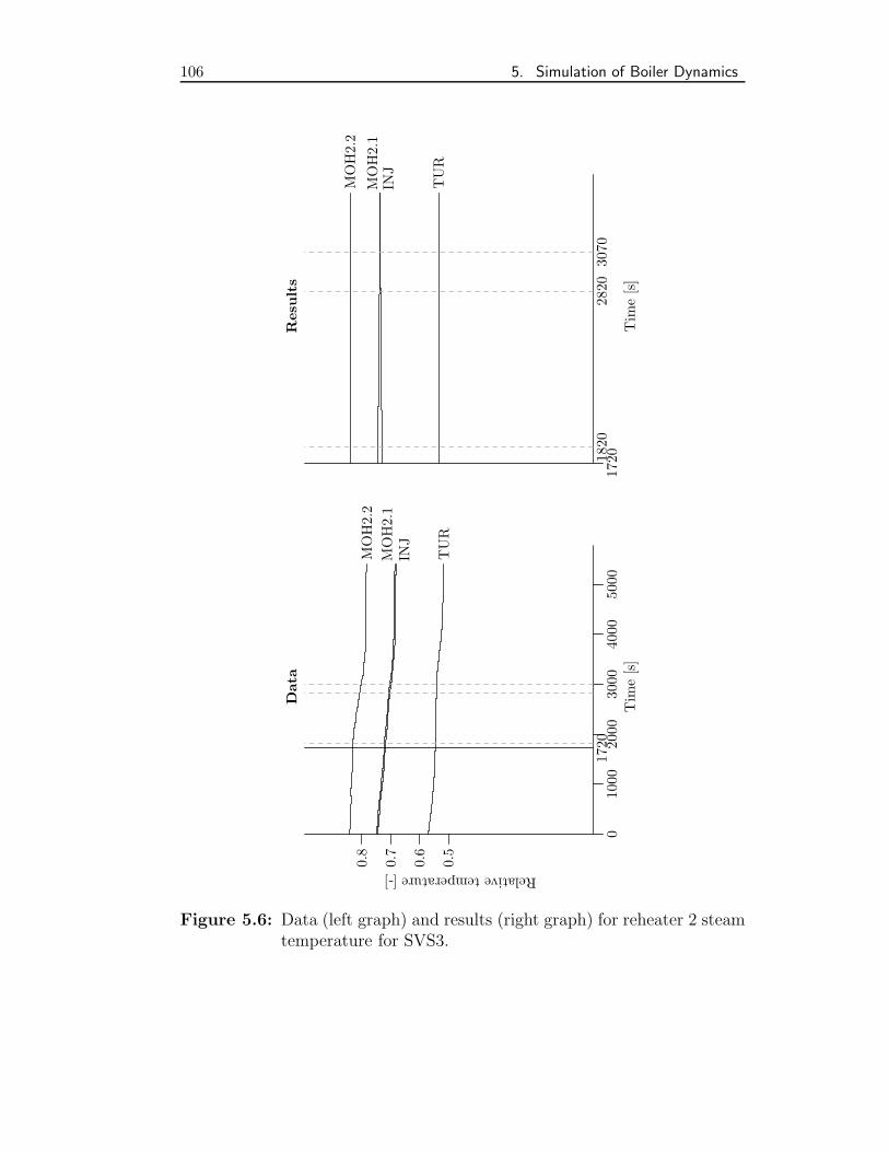
106 5. Simulation of Boiler Dynamics
MOH2.2
INJ
MOH2.1
TUR
01000
2000
3000
4000
5000
0.5
0.6
0.7
0.8
1720
Time[s]
Dat
a
Relativetemperature[-]
TUR
MOH2.1
INJ
MOH2.2
17201820
2820
3070
Time[s]
Res
ult
s
Figure 5.6: Data (left graph) and results (right graph) for reheater 2 steamtemperature for SVS3.
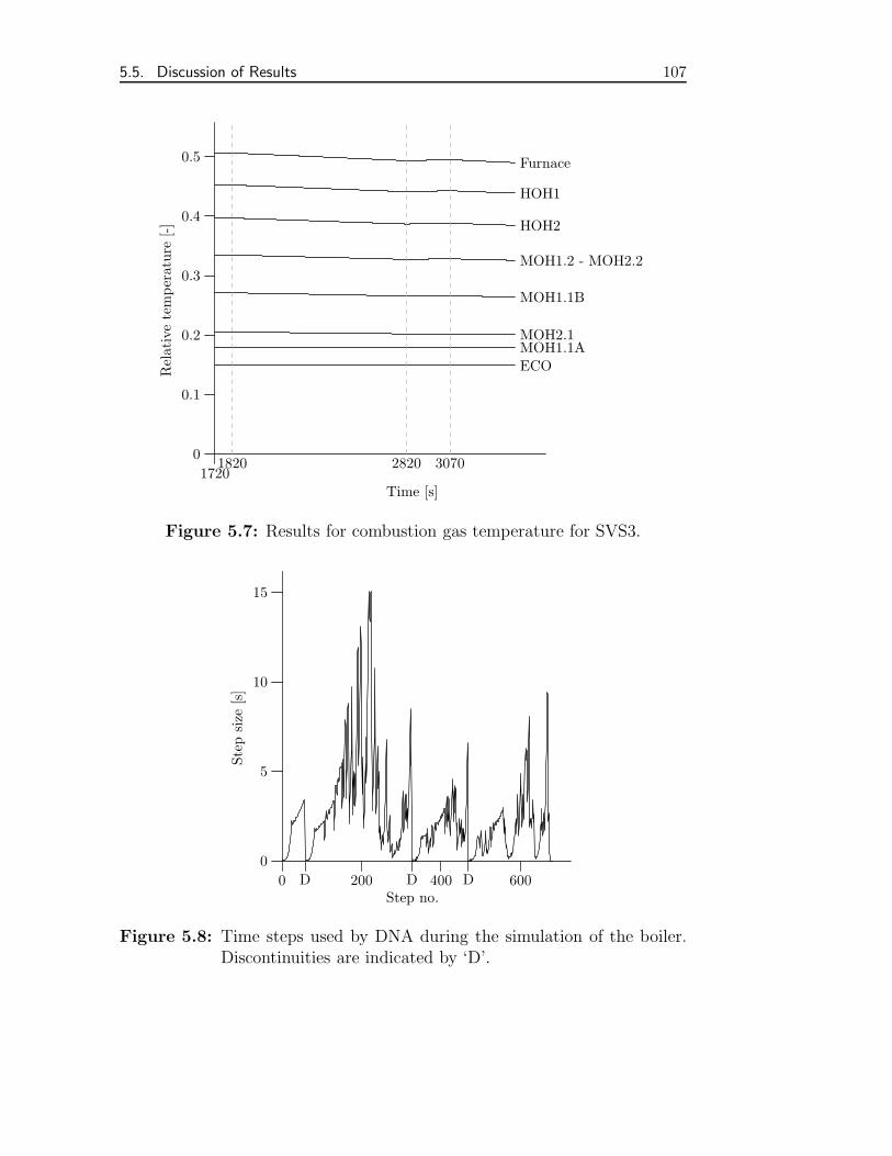
5.5. Discussion of Results 107
Furnace
HOH1
HOH2
MOH1.2 - MOH2.2
MOH1.1B
MOH2.1MOH1.1AECO
0
0.1
0.2
0.3
0.4
0.5
17201820 2820 3070
Time [s]
Relativetemperature[-]
Figure 5.7: Results for combustion gas temperature for SVS3.
0 200 400 6000
5
10
15
D D DStep no.
Step
size[s]
Figure 5.8: Time steps used by DNA during the simulation of the boiler.Discontinuities are indicated by ‘D’.
108 5. Simulation of Boiler Dynamics
to use DNA for prediction of operating characteristics of a given plant, themodel has to extended in several ways.
The primary problems to solve in further extensions of the model are:
• The model should be improved with respect to the modelling of com-bustion reaction and flow of air and fuel in the furnace.
• The models of equipment outside the boiler need to be more extensive.
• DNA should be extended to allow more than two flows to be presentin a component.
6. ANALYSIS OF A BIOMASS-BASEDIGCC PLANT2
6.1 Introduction
Due to the increasing interest in CO2-neutral power production, biomass hasbecome of still higher importance as a fuel. To try to improve the efficiency ofbiomass based plants, it is of interest to utilize biomass in gas turbine plants.This may be done in different ways. In some of these technologies gasificationis a key aspect. For this reason both The Technical University of Denmarkand Delft University of Technology are involved in research aiming at devel-opment of gasifiers for biomass. Therefore, it has been interesting for bothuniversities to have a study which both involved the utilization of biomassgasification in power production and also provided a basis for comparisonof the simulators developed in each university. The study presented in thischapter has been aimed at the utilization of biomass in an IGCC-plant.
An attractive and practicable way of biomass utilization for energy pro-duction is gasification integrated with a combined cycle. This technologyseems to have the possibility to reach high efficiencies based on a fundament-ally clean and renewable fuel. The plants utilize low rank fuels at reasonableoverall efficiencies of up to 50% based on net heating value [6, 15, 81, 100].Integrated biomass gasification/combined cycle plant size is limited by thelow calorific value of the fuel, which also may be very moist. The optimumsize for a specific plant will depend on biomass type and supply and gasturbine adaptability for low calorific value fuels. An integrated biomassgasification/combined cycle plant consists of four major parts. Fuel pre-paration, i.e., drying and/or sizing, gasification, gas turbine and bottomingsteam cycle. These four elemental parts are integrated to exchange heat andthereby raise the overall plant efficiency. This study aims at analyzing andsuggesting improvements for a state-of-the-art integrated biomass gasifica-tion/combined cycle plant.
2 This chapter is based on [32]
110 6. Analysis of a Biomass-based IGCC Plant
6.2 Commercial Integrated BiomassGasification/Combined Cycles
Three gasification plants have been presented as commercially available inliterature. The concepts are all based on air blown fluidized bed gasification,but different approaches to the gasification process are used.
The TPS (Thermal Processes Studsvik) plant is based on gasification atatmospheric pressure. The gasification process takes part in two reactors,one for gasification of the solid fuel and a second reactor for tar crackingwith dolomite as catalyst. Heat for the gasification is supplied by partialcombustion in the reactors, i.e., direct heating. By cooling the gas steamfor the bottoming cycle is generated. Particles are removed from the gasby a bag filter, whereas unwanted gas components such as ammonia andhydrogen sulphide are removed in a wet scrubber. Before entering the com-bustion chamber of the gas turbine the gas is compressed. The plant is bythe developers reported to have an efficiency of up to 45% [6].
The Bioflow (Sydkraft AB and Foster Wheeler) concept is also based ondirect heating, but is accomplished in only one circulating fluid bed reactorat high pressure. The pressure in the gasifier is 25 bar. Tar cracking occursinside the gasifier catalysed by dolomite in the bed. The syngas is cleanedat high temperature. The plant efficiency is between 44% and 50%. [100].
Unlike the two formerly mentioned, the BCL (Battelle Columbus Labor-atory) concept is based on indirectly heated gasification. The syngas produc-tion is split up in two reactors. In the first, the gasifier, biomass is gasified byheat transferred from the bed medium, which is sand. The sand is heated inanother reactor by combustion of the chars that have not been converted inthe gasifier. This process produces a gas with a calorific value of 18 MJ/m3
which is about four times the calorific value of the gas produced by the othergasifiers. This medium-calorific-value gas is usable in more gas turbines thanlow-calorific value gasses. The syngas is cleaned by means of scrubbing. Thisplant configuration leads to an overall efficiency of 36% [81].
A limiting factor for a BIGCC plant is the gas turbine. Few aero-derivative gas turbines, which are attractive because they allow higher tur-bine inlet temperatures, have been proven to run on low calorific value gassesas derived from biomass gasification [105]. One of these is the General Elec-tric LM-2500. This model has been used in former studies because it is of thedesired size and is under development for low calorific value fuels. Fuelledby natural gas it produces 23 MW.
Consonni and Larson [15] have compared the three plant schemes de-scribed above with the GE LM-2500 as basis. The conclusion on their study
6.3. Process Description 111
is that the Bioflow plant has an overall efficiency of 45%, whereas the TPSand BCL plants both have efficiencies of about 42%.
Based on this conclusion which also agrees with the figures referred bythe developers, it has been decided to analyze and suggest improvements forthe most promising plant, the Bioflow cycle, and base the study on the GELM-2500.
6.3 Process Description
The gas turbine compressor should preferably be operated near design loadand it thereby fixes the mass flow of air. Due to the lower calorific value ofthe syngas compared to natural gas the gas turbine expander will operate ata relatively higher mass flow rate. To avoid stall problems, the turbine inlettemperature is lowered from 1232C to about 1100C, to keep the volumeflow at the same level. The outlet temperature from the combustion chamberthen is around 1150C, as the inlet temperature is measured after the firstblade rows [15]. The gasifier temperatures and pressures are determined sothey are appropriate for the pyrolysis and gasification of the fuel reactingwith air. For the Bioflow plant the gasifier is operated at 950–1000C and25 bar [100]. This pressure should also be sufficient to introduce the syngasto the combustion chamber [105]. To obtain the gasification pressure anadditional booster compressor is applied.
Biomass fuels may be rather moist as received. Since the produced syngasmust have a calorific value not lower than about 5 MJ/kg [105], the fuel mayhave to be dried to a moisture content of 10–20%. The dried fuel is bylockhoppers fed to the gasifier.
For pressurized gasification hot gas cleaning is most advantageous. Thetemperature level in the cleaning section is in the range of 300–600C anda reasonable choice of temperature is 500C [18], which is higher than the350C used in [15].
The steam cycle based on a waste heat boiler is laid out with two tur-bine extraction points, one for the deaerator and one for a preheater. Thepressures in the steam cycle are determined by the pinch point temperaturedifferences for the boiler, the preheater and the deaerator.
In the boiler the flue gasses may not be cooled to a temperature below150C, the condensing temperature of sulphuric acid at 1 bar. It seems thatbecause of the low sulphur content of biomass this temperature is not limitingfor the flue gas dryer and the stack [15, 105]. The stack temperature maybe as low as 80C. To regain as much as possible of the energy added to thesystem, it is common to use flue gas drying of the fuel.
112 6. Analysis of a Biomass-based IGCC Plant
6.4 Methods
The modelling of the plant is to large extent based on a base-case modelsimilar to the one of Consonni and Larson [15], but according to recentstudies it has been decided to adjust some of the assumptions [18, 105].In [15, 48, 105] the gasification process has been modelled as a chemicalconverter with specified fuel and syngas composition because the syngas isnot at chemical equilibrium.
In this study an attempt to base the gasification process calculations onequilibrium principles has been made. This leads to a simple model, whichis based on chemical principles.
The base-case model has been analyzed by exergy calculations, which hasestablished the basis of suggestions for improvements of the process design.The system model has been aimed at describing the overall characteristicsof the plant. This is done by lumped parameter assumptions for each of thesystem components.
6.4.1 Simulation Software Applied for the Study
Two software tools, DNA and Cycle-Tempo, have been used for the sim-ulations needed for this study. Both are general energy system simulationtools but they have different features, which has made it interesting to useboth and compare their results. DNA [31, 72] is based on a simultaneousstandard nonlinear equation solver and is easily extended with new compon-ent models. Any quantity including chemical compositions and componentparameters may be used as variables or boundary conditions. These featureshave made it possible to configure the base case system according to thestudy of Consonni and Larson [15] and to find appropriate component para-meters to use in the other simulator Cycle-Tempo which is more convenientfor exergy analysis. Based on the results found with DNA, Cycle-Tempo[66, 76] gives broad possibilities to analyze the plant because the programhas extensive features for analysis of system performance. Among these, ex-ergy calculations are easily carried out. Process schemes presented in thischapter are from the Cycle-Tempo interface and not from DNA. The inputfiles for the model are shown in appendix H.
6.5 Results
The studied system has been simulated in both programs with similar generalsystem characteristics as result. Especially concerning the gasifier differences
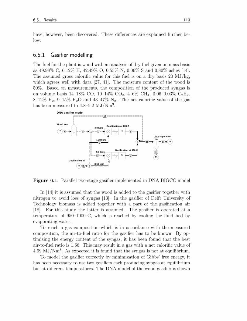
6.5. Results 113
have, however, been discovered. These differences are explained further be-low.
6.5.1 Gasifier modelling
The fuel for the plant is wood with an analysis of dry fuel given on mass basisas 49.98% C, 6.12% H, 42.49% O, 0.55% N, 0.06% S and 0.80% ashes [14].The assumed gross calorific value for this fuel is on a dry basis 20 MJ/kg,which agrees well with data [27, 41]. The moisture content of the wood is50%. Based on measurements, the composition of the produced syngas ison volume basis 14–18% CO, 10–14% CO2, 4–6% CH4, 0.06–0.03% C2Hx,8–12% H2, 9–15% H2O and 43–47% N2. The net calorific value of the gashas been measured to 4.8–5.2 MJ/Nm3.
DNA gasifier model
Gasification at 785 C
Gasification at 390 C
Wood inlet
3.8 kg/s
0.9 kg/s
Ash separation
3.60 kg/s
4.28 kg/s
Gasification air
1
2
34
5
6
7
8
910
11
11 22
33
44
55
66
77
88
99
1010 1111
1212
1313
Figure 6.1: Parallel two-stage gasifier implemented in DNA BIGCC model
In [14] it is assumed that the wood is added to the gasifier together withnitrogen to avoid loss of syngas [13]. In the gasifier of Delft University ofTechnology biomass is added together with a part of the gasification air[18]. For this study the latter is assumed. The gasifier is operated at atemperature of 950–1000C, which is reached by cooling the fluid bed byevaporating water.
To reach a gas composition which is in accordance with the measuredcomposition, the air-to-fuel ratio for the gasifier has to be known. By op-timizing the energy content of the syngas, it has been found that the bestair-to-fuel ratio is 1.66. This may result in a gas with a net calorific value of4.99 MJ/Nm3. As expected it is found that the syngas is not at equilibrium.
To model the gasifier correctly by minimization of Gibbs’ free energy, ithas been necessary to use two gasifiers each producing syngas at equilibriumbut at different temperatures. The DNA model of the wood gasifier is shown
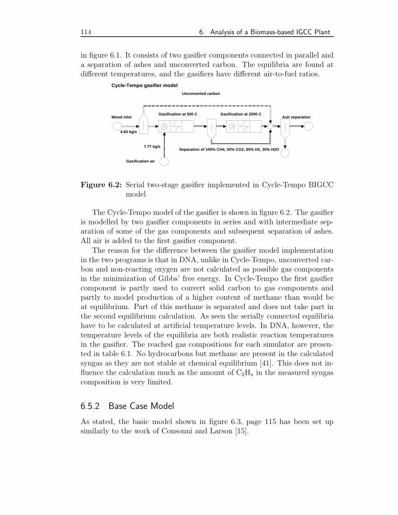
114 6. Analysis of a Biomass-based IGCC Plant
in figure 6.1. It consists of two gasifier components connected in parallel anda separation of ashes and unconverted carbon. The equilibria are found atdifferent temperatures, and the gasifiers have different air-to-fuel ratios.
Cycle-Tempo gasifier model
Gasification at 500 C Gasification at 2000 CWood inlet
4.60 kg/s
Ash separation
7.77 kg/s
Gasification air
Unconverted carbon
Separation of 100% CH4, 50% CO2, 60% H2, 30% H2O
Figure 6.2: Serial two-stage gasifier implemented in Cycle-Tempo BIGCCmodel
The Cycle-Tempo model of the gasifier is shown in figure 6.2. The gasifieris modelled by two gasifier components in series and with intermediate sep-aration of some of the gas components and subsequent separation of ashes.All air is added to the first gasifier component.
The reason for the difference between the gasifier model implementationin the two programs is that in DNA, unlike in Cycle-Tempo, unconverted car-bon and non-reacting oxygen are not calculated as possible gas componentsin the minimization of Gibbs’ free energy. In Cycle-Tempo the first gasifiercomponent is partly used to convert solid carbon to gas components andpartly to model production of a higher content of methane than would beat equilibrium. Part of this methane is separated and does not take part inthe second equilibrium calculation. As seen the serially connected equilibriahave to be calculated at artificial temperature levels. In DNA, however, thetemperature levels of the equilibria are both realistic reaction temperaturesin the gasifier. The reached gas compositions for each simulator are presen-ted in table 6.1. No hydrocarbons but methane are present in the calculatedsyngas as they are not stable at chemical equilibrium [41]. This does not in-fluence the calculation much as the amount of C2Hx in the measured syngascomposition is very limited.
6.5.2 Base Case Model
As stated, the basic model shown in figure 6.3, page 115 has been set upsimilarly to the work of Consonni and Larson [15].
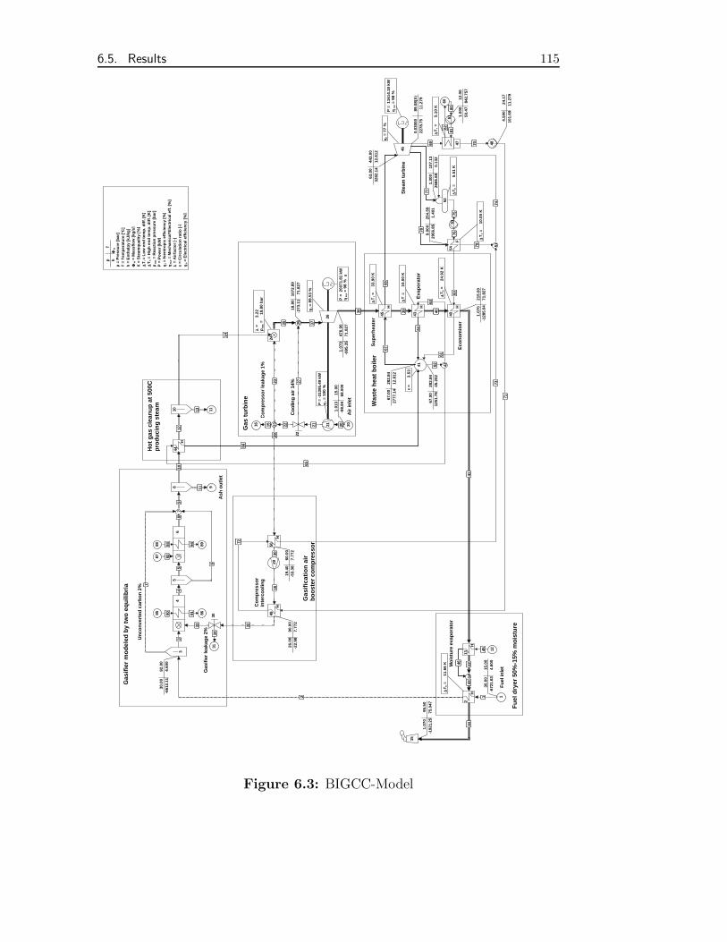
6.5. Results 115
P =
116
14.1
8 kW
ηηm
,e =
98
%
P =
200
71.8
1 kW
η ηm
,e =
98
%
∆∆T
h =
1
1.66
K
P =
-31
395.
49 k
Wηη
e =
100
%
λλ =
3.
22p
reac
=
18.
80 b
ar
ηηi =
89.
53 %
∆∆T
h =
2
4.92
K
x =
3.
53∆∆
Tl =
1
0.00
K
∆∆T
h =
3
3.90
K
ηηi =
77
%
∆∆T
h =
5.10
K
∆∆T
h =
5.51
K
∆∆T
h =
1
0.00
K
pT
hΦΦ
m
p =
Pre
ssu
re [
bar
]T
= T
emp
erat
ure
[°C
]h
= E
nth
alp
y [k
J/kg
]ΦΦ
m =
Mas
sflo
w [
kg/s
]X
= S
team
qu
alit
y [%
]∆∆
Tl =
Lo
w e
nd
tem
p. d
iff.
[K]
∆∆T
h =
Hig
h e
nd
tem
p. d
iff.
[K]
pre
ac =
Rea
ctio
n p
ress
ure
[b
ar]
P =
Po
wer
[kW
]ηη
i = Is
entr
op
ic e
ffic
ien
cy [
%]
ηηm
,e =
Mec
han
ical
*Ele
ctri
cal e
ff. [
%]
λλ =
Air
fact
or
[-]
x =
Cir
cula
tio
n r
atio
[-]
ηηe =
Ele
ctri
cal e
ffic
ien
cy [
%]
Fu
el d
ryer
50%
-15%
mo
istu
re
Un
con
vert
ed c
arb
on
2%
Ash
ou
tlet
Gas
ifie
r m
od
eled
by
two
eq
uili
bri
a
Ho
t g
as c
lean
up
at
500C
pro
du
cin
g s
team
Gas
tu
rbin
e
Was
te h
eat
bo
iler
Gas
ific
atio
n a
ir
bo
ost
er c
om
pre
sso
r
Ste
am t
urb
ine
Fu
el in
letM
ois
ture
eva
po
rato
r
Air
inle
t
Co
mp
ress
or
leak
age
1%
Gas
ifier
leak
age
2%
Co
olin
g a
ir 1
4%
#
Su
per
hea
ter
Eva
po
rato
r
Eco
no
mis
er
Co
mp
ress
or
inte
rco
olin
g
1
2
H
34
56
78 9
10 11
12
13
H14
15
16 2021
22
2324
25
26
29
3031
40
H
41 42
43
H
44
H
45
H
46
47 48
49
H
50
H
51
52
5354
F
6061
85 86
8788 89
11
30.
00
15.
00 -6
721.
63
4.6
00
22
3
0.00
9
2.00
-661
2.11
4
.600
3344
55
66
77
8899
1010
1111
1212
1313
1414
1515
1616
2020
1.0
13
15.
00
-98.
84
68.0
00
21212222
2323 2727
29293030
1
9.40
6
0.00
-5
3.38
7
.772
3232
2
6.00
9
0.00
-2
2.98
7
.7723333
3434
3535 3737
1
8.80
107
2.89
-27
3.11
71
.827
3838
1
.070
47
6.90
-99
5.35
71
.827
3939 4040
4141
1
.070
21
5.00
-128
5.04
71
.827
42424343
4444
1
.070
9
5.50
-192
1.25
75
.047
4545
46466060
6161
6262
67.
00
282.
84 1
251.
78
45.2
026363
6464
6565
6666
6767
67.
00
282.
84 2
777.
14
12.8
12
6868
6
3.00
44
3.00
328
2.14
12
.812
6969
0.0
3000
8
9.08
(X)
227
8.75
11
.279
7070
7171
4.5
00
24.
17
101.
69
11.2
79
7272
73737474
75757676
7777
1.3
00
107.
13 2
686.
68
0.1
32
7878
9
.000
25
4.59
295
6.85
1
.401
7979
8080
1
.000
1
2.00
5
0.47
842
.757
8181
8282
9090 9191
92929393 9494
Figure 6.3: BIGCC-Model
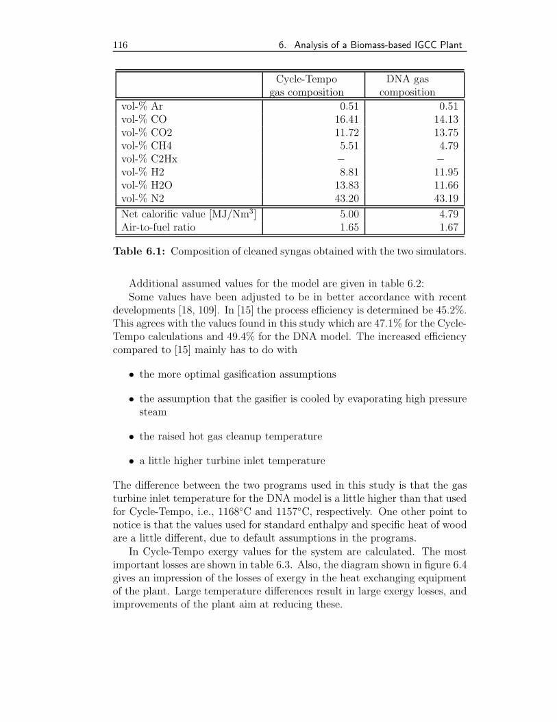
116 6. Analysis of a Biomass-based IGCC Plant
Cycle-Tempogas composition
DNA gascomposition
vol-% Ar 0.51 0.51vol-% CO 16.41 14.13vol-% CO2 11.72 13.75vol-% CH4 5.51 4.79vol-% C2Hx − −vol-% H2 8.81 11.95vol-% H2O 13.83 11.66vol-% N2 43.20 43.19
Net calorific value [MJ/Nm3] 5.00 4.79Air-to-fuel ratio 1.65 1.67
Table 6.1: Composition of cleaned syngas obtained with the two simulators.
Additional assumed values for the model are given in table 6.2:Some values have been adjusted to be in better accordance with recent
developments [18, 109]. In [15] the process efficiency is determined be 45.2%.This agrees with the values found in this study which are 47.1% for the Cycle-Tempo calculations and 49.4% for the DNA model. The increased efficiencycompared to [15] mainly has to do with
• the more optimal gasification assumptions
• the assumption that the gasifier is cooled by evaporating high pressuresteam
• the raised hot gas cleanup temperature
• a little higher turbine inlet temperature
The difference between the two programs used in this study is that the gasturbine inlet temperature for the DNA model is a little higher than that usedfor Cycle-Tempo, i.e., 1168C and 1157C, respectively. One other point tonotice is that the values used for standard enthalpy and specific heat of woodare a little different, due to default assumptions in the programs.
In Cycle-Tempo exergy values for the system are calculated. The mostimportant losses are shown in table 6.3. Also, the diagram shown in figure 6.4gives an impression of the losses of exergy in the heat exchanging equipmentof the plant. Large temperature differences result in large exergy losses, andimprovements of the plant aim at reducing these.
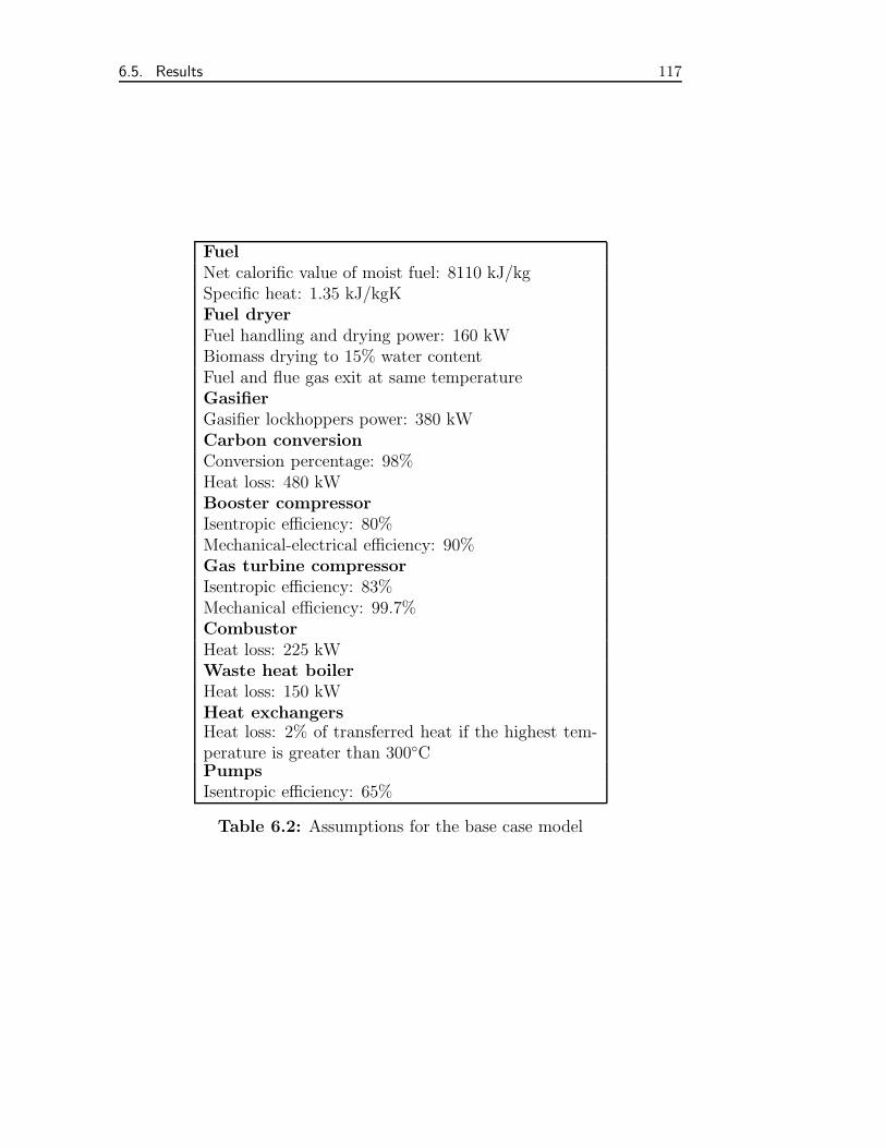
6.5. Results 117
FuelNet calorific value of moist fuel: 8110 kJ/kgSpecific heat: 1.35 kJ/kgKFuel dryerFuel handling and drying power: 160 kWBiomass drying to 15% water contentFuel and flue gas exit at same temperatureGasifierGasifier lockhoppers power: 380 kWCarbon conversionConversion percentage: 98%Heat loss: 480 kWBooster compressorIsentropic efficiency: 80%Mechanical-electrical efficiency: 90%Gas turbine compressorIsentropic efficiency: 83%Mechanical efficiency: 99.7%CombustorHeat loss: 225 kWWaste heat boilerHeat loss: 150 kWHeat exchangersHeat loss: 2% of transferred heat if the highest tem-perature is greater than 300CPumpsIsentropic efficiency: 65%
Table 6.2: Assumptions for the base case model
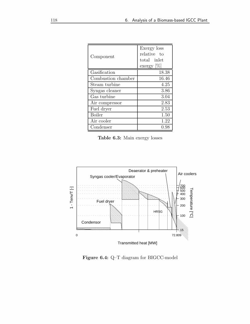
118 6. Analysis of a Biomass-based IGCC Plant
Component
Exergy lossrelative tototal inletexergy [%]
Gasification 18.38Combustion chamber 16.46Steam turbine 4.25Syngas cleaner 3.86Gas turbine 3.04Air compressor 2.83Fuel dryer 2.53Boiler 1.50Air cooler 1.22Condenser 0.98
Table 6.3: Main exergy losses
100
200
300
400500600700
Air coolers
HRSG
Deaerator & preheater
Syngas cooler/Evaporator
Fuel dryer
Condensor
15
Tem
perature [°C]
1 -
Ten
v/T
[-]
72.8090
Transmitted heat [MW]
Figure 6.4: Q–T diagram for BIGCC-model
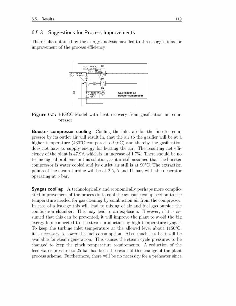
6.5. Results 119
6.5.3 Suggestions for Process Improvements
The results obtained by the exergy analysis have led to three suggestions forimprovement of the process efficiency:
∆∆ Tl = 55.54 K∆∆ Th = 60.69 K
P = -316.98 kWηη i = 79.86 %ηη m,e = 90 %
∆∆ Tl = 35.83 K∆∆ Th = 85.54 K
∆∆ Tl = 30.00 K∆∆ Th = 35.27 K
Gasification air booster compressor
17
H
29
49
H
50
H
22
1616
1818
1919
2424
2525
3232
Figure 6.5: BIGCC-Model with heat recovery from gasification air com-pressor
Booster compressor cooling Cooling the inlet air for the booster com-pressor by its outlet air will result in, that the air to the gasifier will be at ahigher temperature (430C compared to 90C) and thereby the gasificationdoes not have to supply energy for heating the air. The resulting net effi-ciency of the plant is 47.9% which is an increase of 1.7%. There should be notechnological problems in this solution, as it is still assumed that the boostercompressor is water cooled and its outlet air still is at 90C. The extractionpoints of the steam turbine will be at 2.5, 5 and 11 bar, with the deaeratoroperating at 5 bar.
Syngas cooling A technologically and economically perhaps more complic-ated improvement of the process is to cool the syngas cleanup section to thetemperature needed for gas cleaning by combustion air from the compressor.In case of a leakage this will lead to mixing of air and fuel gas outside thecombustion chamber. This may lead to an explosion. However, if it is as-sumed that this can be prevented, it will improve the plant to avoid the bigexergy loss connected to the steam production by high temperature syngas.To keep the turbine inlet temperature at the allowed level about 1150C,it is necessary to lower the fuel consumption. Also, much less heat will beavailable for steam generation. This causes the steam cycle pressures to bechanged to keep the pinch temperature requirements. A reduction of thefeed water pressure to 25 bar has been the result of this change of the plantprocess scheme. Furthermore, there will be no necessity for a preheater since
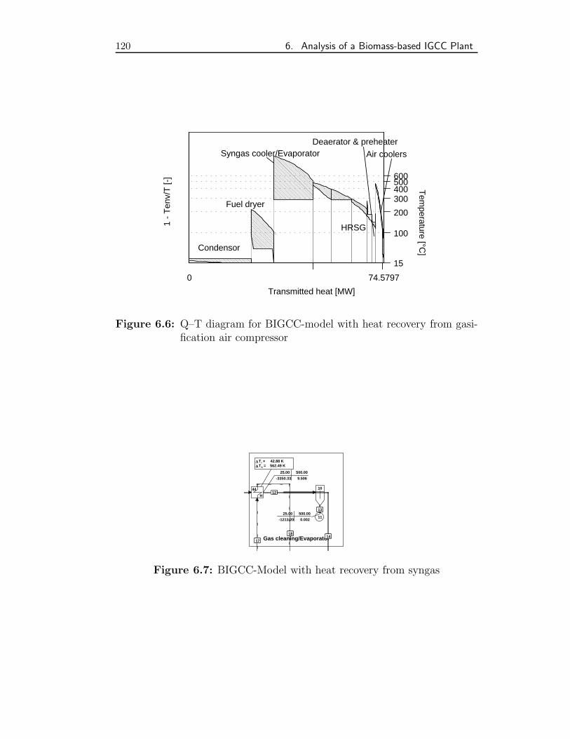
120 6. Analysis of a Biomass-based IGCC Plant
100
200
300400500600
Air coolers
HRSG
Deaerator & preheaterSyngas cooler/Evaporator
Fuel dryer
Condensor
15
Tem
perature [°C]
1 -
Ten
v/T
[-]
74.57970
Transmitted heat [MW]
Figure 6.6: Q–T diagram for BIGCC-model with heat recovery from gasi-fication air compressor
∆∆ Tl = 42.88 K∆∆ Th = 562.49 K
Gas cleaning/Evaporator
10
11
44
H1212
25.00 500.00
-3350.33 9.506
1313 25.00 500.00
-1213.20 0.002
14141717
1818
Figure 6.7: BIGCC-Model with heat recovery from syngas
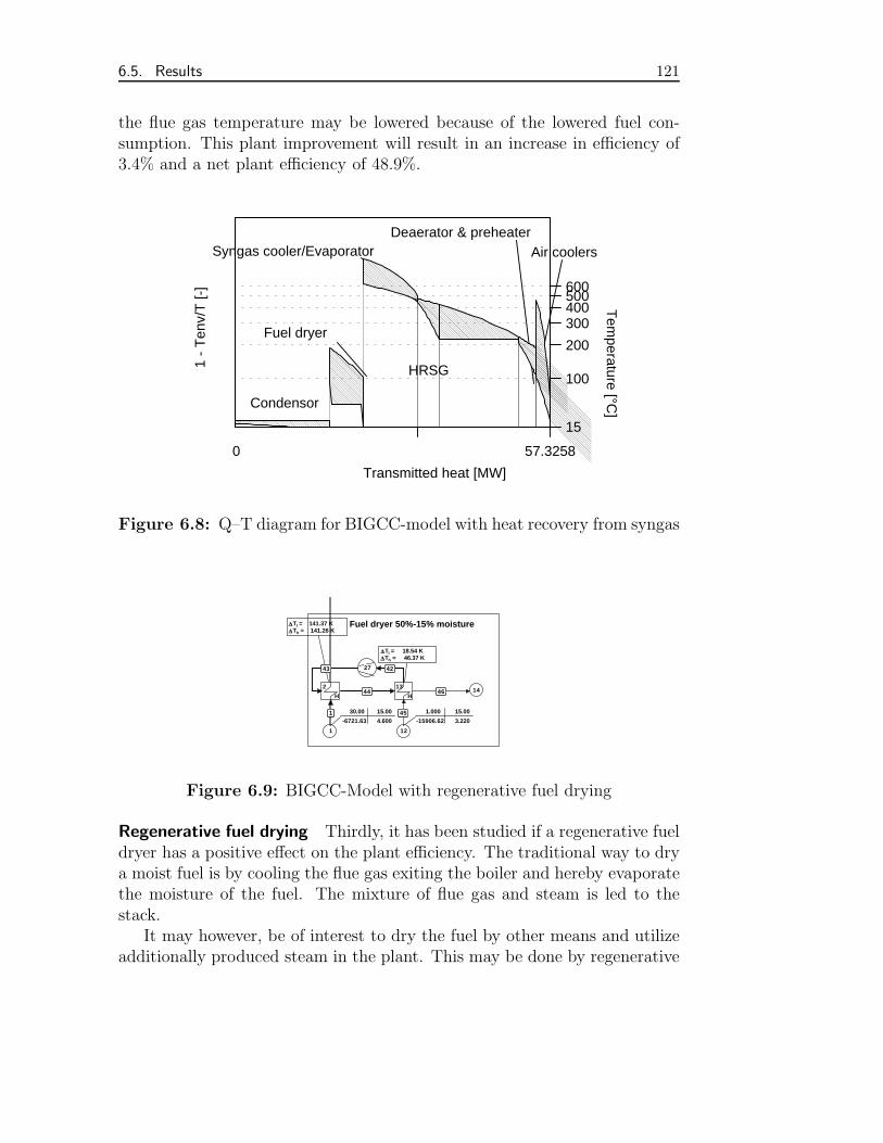
6.5. Results 121
the flue gas temperature may be lowered because of the lowered fuel con-sumption. This plant improvement will result in an increase in efficiency of3.4% and a net plant efficiency of 48.9%.
100
200
300400500600
Air coolers
HRSG
Deaerator & preheaterSyngas cooler/Evaporator
Fuel dryer
Condensor
15
Tem
perature [°C]
1 -
Ten
v/T
[-]
57.32580
Transmitted heat [MW]
Figure 6.8: Q–T diagram for BIGCC-model with heat recovery from syngas
∆∆ Tl = 141.37 K∆∆ Th = 141.26 K
∆∆ Tl = 18.54 K∆∆ Th = 46.37 K
Fuel dryer 50%-15% moisture
1
2
H
12
13
H14
27
11 30.00 15.00
-6721.63 4.600
42424343
4444
4545 1.000 15.00
-15906.62 3.220
4646
Figure 6.9: BIGCC-Model with regenerative fuel drying
Regenerative fuel drying Thirdly, it has been studied if a regenerative fueldryer has a positive effect on the plant efficiency. The traditional way to drya moist fuel is by cooling the flue gas exiting the boiler and hereby evaporatethe moisture of the fuel. The mixture of flue gas and steam is led to thestack.
It may however, be of interest to dry the fuel by other means and utilizeadditionally produced steam in the plant. This may be done by regenerative
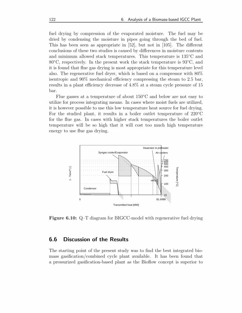
122 6. Analysis of a Biomass-based IGCC Plant
fuel drying by compression of the evaporated moisture. The fuel may bedried by condensing the moisture in pipes going through the bed of fuel.This has been seen as appropriate in [52], but not in [105]. The differentconclusions of these two studies is caused by differences in moisture contentsand minimum allowed stack temperatures. This temperature is 135C and80C, respectively. In the present work the stack temperature is 93C, andit is found that flue gas drying is most appropriate for this temperature levelalso. The regenerative fuel dryer, which is based on a compressor with 80%isentropic and 90% mechanical efficiency compressing the steam to 2.5 bar,results in a plant efficiency decrease of 4.8% at a steam cycle pressure of 15bar.
Flue gasses at a temperature of about 150C and below are not easy toutilize for process integrating means. In cases where moist fuels are utilized,it is however possible to use this low temperature heat source for fuel drying.For the studied plant, it results in a boiler outlet temperature of 220Cfor the flue gas. In cases with higher stack temperatures the boiler outlettemperature will be so high that it will cost too much high temperatureenergy to use flue gas drying.
100
200
300
400500600700
Air coolers
HRSG
Deaerator & preheater
Syngas cooler/Evaporator
Fuel dryer
Condensor
15
Tem
perature [°C]
1 -
Ten
v/T
[-]
81.69880
Transmitted heat [MW]
Figure 6.10: Q–T diagram for BIGCC-model with regenerative fuel drying
6.6 Discussion of the Results
The starting point of the present study was to find the best integrated bio-mass gasification/combined cycle plant available. It has been found thata pressurized gasification-based plant as the Bioflow concept is superior to
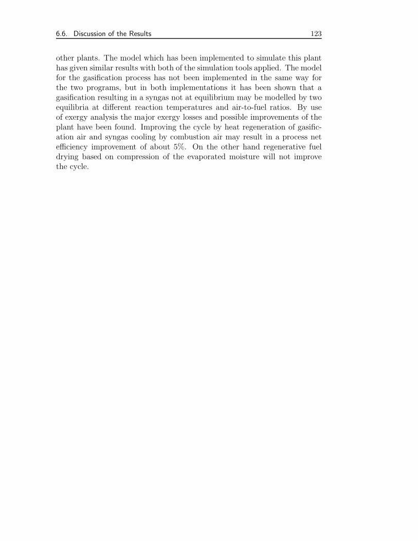
6.6. Discussion of the Results 123
other plants. The model which has been implemented to simulate this planthas given similar results with both of the simulation tools applied. The modelfor the gasification process has not been implemented in the same way forthe two programs, but in both implementations it has been shown that agasification resulting in a syngas not at equilibrium may be modelled by twoequilibria at different reaction temperatures and air-to-fuel ratios. By useof exergy analysis the major exergy losses and possible improvements of theplant have been found. Improving the cycle by heat regeneration of gasific-ation air and syngas cooling by combustion air may result in a process netefficiency improvement of about 5%. On the other hand regenerative fueldrying based on compression of the evaporated moisture will not improvethe cycle.

124 6. Analysis of a Biomass-based IGCC Plant
7. CONCLUSION
This study has focussed on extension of the DNA simulator, in order tobe able to use the program in simulation of the two case studies covered,i.e., boiler dynamics and design of a BIGCC plant. During the developmenta number of features of DNA have been evaluated and extended as necessary.The conclusions of the study are made based on the experiences from thisdevelopment. Therefore, it is in this conclusion taken as a fact that thebasic implementation and theory of DNA is well suited for energy systemsimulation. The present work has extended the features of DNA and hasprovided both a deeper insight in the implementation of simulation programsfor energy systems. Also it has revealed some of the weaker parts of theoryand assumptions applied in the development of DNA.
Below the results of the work on DNA are taken as basis and are gener-alized for application in the context of energy system simulation software.
The main results of the present study can be divided into groups accordingto the three topics outlined in the title, i.e., development, evaluation andapplication of DNA. The three topics cannot, however, be distinguished easilyin the work, as they each involve one or more parts of the modelling process,which is indeed an iterative procedure.
7.1 Basis for the Present Work
The basis for the work has naturally been the existing features of the DNAcode. To summarize, DNA was, and is, a highly flexible and in many waysunique program. The primary reasons for this statement is that DNA dur-ing previous projects has been developed according to what in this work hasbeen termed as the PREFUR framework, where PREFUR is an acronym forPortability, Robustness, Efficiency, Flexibility, User Friendliness and Read-ability of the code. The previous works of Perstrup [82] and Lorentzen [72]have mainly aimed at the selection and implementation of basic features forsome of the items. These works have made DNA portable between operat-ing systems, flexibly applicable to virtually any, simple energy system andefficiently solving the system of equations formed by a model.
Perstrup first of all did the basic implementation of the code based on a
126 7. Conclusion
highly modular methodology, originating in an application of network theoryto thermodynamic processes, i.e., energy systems. The work aimed at writinga code for simulation of steady state models. In order to simulate a modelof a given system, Perstrup implemented simple models of equipment com-monly used in energy systems, a numeric solver and routines for calculationof thermodynamic properties of water, steam and gas. A very important fa-cility of the program is the possibility for inclusion of new component modelsin an easy way.
Lorentzen extended the code in many ways mainly aiming at implement-ation of features for simulation of dynamic processes. This work involvedselection and implementation of facilities for solving a system of differential-algebraic equations. This is handled in an elegant way by formulating thedifferential equations, so they can be solved in conjunction with the algebraicequations. Also, handling of time dependent discontinuities was included. Tosimulate a broader class of systems, extended expressions for thermodynamicproperties of ideal gases were included in the code.
7.2 Implementation of Features in Energy SystemSimulators
The initial task of the present work was to determine which items had to beaddressed in order to fulfill the main objective of the study, i.e., to model andsimulate the dynamic behaviour of a complicated energy system, exemplifiedby a modern power plant boiler. Additionally, the other main simulationstudy, the biomass-based IGCC plant revealed deficiencies of the DNA code.Primarily, it was found that the simulation of the systems required imple-mentation of additional and in some cases much more complicated compon-ent models than already present in the library of DNA. For simulation ofboiler dynamics, mainly the following component models have been foundnecessary:
• The basic model for heat exchange based on a specified or a calculatedheat transfer coefficient has been improved with respect to robustness.This model has been used as basis for other heat exchanger models,e.g., the ones used in the boiler model. The study of the heat exchangermodel has shown that it is possible to extend constrained applicablecomponent models to make them robustly usable in simulations.
• Furnace for steady and transient processes. The furnace has comparedto other codes not been based on the assumption that the furnace isone single lumped model. The implemented model may be subdivided,
7.2. Implementation of Features in Energy System Simulators 127
due to the inclusion of transparent border walls between parts of thecomponent. This makes the model highly flexible. In future studiesdivision in two or three dimensions may be assessed.
• Crossflow heat exchangers with and without finned tubes for applic-ation as superheaters in both steady state and transient simulations.The model includes both radiant and convective heat transfer. The ra-diative transfer is based on application of transparent borders also. Thecross flow correction factor has been analyzed for robust applicabilityin simulators.
And for the BIGCC simulation:
• A solid fuel gasifier has been required in the model. The model hasbeen implemented, such that it allows a program to exploit the featuresof a general numerical solver. This is an important improvement withrespect to efficiency of the solution.
• A solid fuel dryer has been implemented and handles both heating offuel, evaporation of water and calculation of the resulting fuel compos-ition.
• A gas cleaning section has been implemented as a generally applicableseparator.
• A gas mixer has, similarly, been implemented in a general way.
For both applications relevant utility components have been improved to takeadvantage of newly implemented features of the code.
7.2.1 Features for Component Models
In order to implement the models, it was essential to include features for:
• evaluation of transport properties of relevant fluids
• evaluation of radiative properties of relevant fluids
• evaluation of relevant dimensionless quantities for calculation of frictionfactors and heat transfer coefficients
• evaluation of heat transfer coefficients and friction coefficients for flowinside tubes and in tube banks of finned and unfinned tubes
128 7. Conclusion
• evaluation of relevant view factors for radiative heat transfer betweensurfaces in boilers
• evaluation of thermo-physical properties of solid fuels and ashes
All of these features have been found to be required for a simulator whichshould be considered to be generally applicable in energy system studies.These facilities have been included as separate routines in the code, allowingcoming users to apply them in other component models. The properties havebeen selected as the best available in literature.
7.3 General Considerations on the Implementation ofSimulators
General extensions of the features of DNA have been carried out, in order toimprove all of the points of the PREFUR framework.
The main philosophy behind these extensions is, that user friendlinessis a primary property, which is to some extent a result of the other termsof of PREFUR. Accordingly, user friendliness of a program will be greatlyimproved if
• the numerical solver itself and the component models are both robust,efficient and flexible
• the flexibility of component models is at a high level
• the amount of work required from the user is kept at the lowest possiblelevel
The main results of the development of DNA may be summarized by thefollowing items:
• Subdivision of component models allows for both simpler system formu-lations and more accurate calculations of relevant features of a system.A very high flexibility of the component models may be implementeddue to this extension. Component models may now be implementedto span from fully lumped parameter models to models distributed inthree dimensions and with a user-specified number of equations andbranches.
• Allowance for media specification to be done in a robust way in thesystem model, and not in the components models routines, has consid-erably lowered the number of component routines present in the code,
7.4. Comparison of DNA to Other Codes 129
and the demand for implementation of component models during mod-elling work. That a medium had to be predefined in the componentmodels for all branches seems to be a bad assumption of the previousdevelopments of DNA. There is no physical relevance in the previouslyapplied methodology. Instead groups of media are now allowed in eachbranch. This makes component models much more general.
• Generation of initial guesses for the numerical solver based on firstprinciples and component-specific features has decreased the requiredwork from the user and has at the same time made the solution processmore robust and easier convergent, because the variables have suitableinitial values. This feature makes the application of a simultaneousequation solver in a simulation program more reliable and attractive.
• Handling of variable-dependent discontinuities has been included tomake the code applicable in simulation of a large class of dynamic sys-tems including different control systems. The use of DNA in ‘virtuallyany’ energy system is now possible. The implementation has been madeso no numerical calculations are required for the interpolation to im-prove the accuracy of the obtained results by additional calculations.Also, the method may not be initialized in a wrong state by the user,as DNA will recalculate the problem, if this occurs.
7.4 Comparison of DNA to Other Codes
The work with DNA and Cycle-Tempo on the same model has providedthe main basis for an evaluation of DNA. One result of this comparison is,that features lacking in DNA have been included. Other comparisons ofthis kind in the future may provide additional valuable inspiration for newdevelopments of DNA.
Literature on other codes has also been taken into account for an evalu-ation of the usefulness of DNA in practical applications. The primary con-clusion of this evaluation is that DNA have superior features compared toother codes, because it from the beginning has been developed to be generallyapplicable and extendible. Features to emphasize in this context are
• the numerical routines applied for both steady state and dynamic mod-els including handling of discontinuities, which are both general, flexibleand efficient.
• the robust internal model description, which makes handling of algeb-raic loops and energy balances easy and, additionally, has allowed the
130 7. Conclusion
implementation of a feature for generation of initial guesses.
In order to make DNA available to a broader audience, however, a graphicaluser interface is mandatory. Without this it will be very difficult to advertizeDNA as a user friendly program.
7.5 Suggestions for Future Extensions of DNA
Throughout this thesis, DNA has been claimed to have unique features andto be a very promising tool for engineers working with energy system studiesin virtually any field. However, the program has only been applied in a fewstudies compared to notable commercial codes. Furthermore, most of thesestudies have focussed on system layout applying highly simplified models forthe devices. To see if the program is as good as claimed, I highly recommendthat future studies approach modelling and improvement of existing or futureindustrial installations.
Graphical User Interface A graphical user interface should have a highpriority in the coming work on DNA, because it will allow the programto be easier to approach for new users, also in industry. The more users,the more suggestions for improvement of the code may be obtained, andthe code will eventually be a very powerful tool.
Controlling the Numerical Solution It has been found that the robust-ness of the model may be improved by introduction of generally validequations. The solver, however, still has to be controlled carefully. Im-plementation of a ‘globally convergent’ solver or some automatic controlof the Newton method may be considered.
Equation Parser To allow users to use models which have not been com-piled into the code, it will be necessary to include an interpreter fora component model. This will necessarily have to include an equationparser.
Component Library The component library should steadily be improvedand extended. As constitutive relations for fluid flowing in circularpipes are applied in many component, a collection of routines for suchstandard relations might be written and used by several componentmodels.
Dynamic Shafts The facility for simulation of shaft rotation in a turbinehas not been applied. This needs to be done.
7.6. Applications of DNA 131
Programming the Code As is, DNA is written in ANSI standard FOR-TRAN77, almost without exception. Translation of DNA to the newfree-form FORTRAN90 standard would not only allow a neater lookingcode to be written, but also allow the main new features of the newstandard to be exploited.
7.6 Applications of DNA
7.6.1 Boiler Dynamics
The application of DNA to simulation of boiler dynamics has first of allproven, that DNA is useful for this purpose. From a modelling viewpoint, acomprehensive analysis of radiative heat transfer in furnaces and in super-heater sections has been implemented with well-known relations for convect-ive heat transfer and pressure loss. The furnace model is flexible and may besubdivided to obtain information about the thermodynamic state at differentlocations inside of it. The furnace model do have deficiencies. Combustion isassumed to be instantaneous and therefore the distribution and flow of air,fuel and combustion products in the furnace is neglected. Unfortunately, thismakes the subdivision of the furnace model difficult to apply.
The results of the actual simulations of a load-change of the SkærbækPlant Unit 3 has shown that the model is capable of reproducing the trendsof the dynamic behaviour of the boiler. To obtain better results, it will benecessary to develop the model to have a better knowledge about the rest ofthe plant, including turbines, preheaters and control system.
7.6.2 Biomass-based IGCC Plant
The optimization study of a BIGCC process resulted in the formulation ofa multi-stage chemical equilibrium model of gasification. This approach wasuseful, because both DNA and Cycle-Tempo had a chemical equilibriummodel available as a gasifier model, but chemical equilibrium is not obtainedin biomass fluid bed gasifiers.
The study resulted in suggestions for improvement of the plant design.The best of these give a possible increase of 5% of the plant efficiency.
For DNA, the modelling resulted in the implementation of handling ofsolid fuels and the development of a chemical equilibrium model for solids.The gasifier model has been optimized for application in the overall numericalsolver. This has proven to be advantageous with respect to efficiency of thesolution procedure.
132 7. Conclusion
It is hoped that also the future development of Cycle-Tempo may takeadvantage of the results of the present study.
7.7 Final statement
The conclusion on this work is that:
DNA has during the present work been extended in severalways to be able to simulate more complex systems. The exten-sions have improved the code with respect to the items of thePREFUR framework.
New features have been added to the code. These are gener-ally made available as separate routines which may be accessed byany model as needed. The application of these features in simu-lation of power plant boiler dynamics and design of a BIGCC hasshown the practical use of DNA for studies of complex systems.
The results of the boiler study have shown that models formu-lated for and simulated with DNA can reproduce measurementsfrom working energy systems.
Quoting Bent Lorentzen it may be concluded that
“All in all[ . . . ]that DNA is a unique, fast and flexiblesimulation tool for power plant simulation.”
The work of the present study supports the possibility formaking this conclusion generally accepted among a broader audi-ence, due to addition of features improving the code in manyways.
Also, the methods implemented in DNA may be advantage-ously applied in the development of other simulation codes in thefield.
BIBLIOGRAPHY
[1] M. Abramowitz and I. A. Stegun. Handbook of Mathematical Functions.Dover Publications, Inc., ninth printing, 1972.
[2] E. Allgower and K. Georg. Simplicial and Continuation Methods forApproximating Fixed Points and Solutions to Systems of Equations.SIAM Review, 22(1):28–85, jan 1980.
[3] C. R. Altafini and A. Mirandola. A Chemical Equilibrium Model ofthe Coal Gasification Process Based on the Minimization of the GibbsFree Energy. In Manfrida [75], pages 419–427.
[4] M. Assadi, P. Rosen and N. Agren. Utvardering av olikavarmebalansprogram, (Comparison of different Heat balance pro-grams). Technical Report LUTMDN/TMVK–3173–SE, Departmentof Heat and Power Engineering, Lund Institute of Technology, Sweden,1995.
[5] C. Bendtsen and P. G. Thomsen, editors. Numerical Simulation of Dif-ferential Algebraic Equations. Number IMM-REP-1999-8. Departmentof Mathematical Modelling, Technical University of Denmark, 1999.
[6] W. H. Blackadder, H. Lundberg, E. Rensfelt and L. Waldheim. Heatand Power Production via Gasification in the Range 5–50 MWe. InA. V. Bridgwater, editor, Advances in Thermochemical Biomass Con-version, pages 449–475. Blackie, 1994.
[7] A. G. Blokh. Heat Transfer in Steam Boiler Furnaces. HemispherePublishing Corporation, 1988.
[8] F. Brandt. Warmeubertragung in Dampferzeugern und Warmeaustau-schern, volume 2 of FBDR–Fachbuchreihe. Fachverband Dampfkessel-,Behalter- und Rohrleitungsbau E.V., 1985.
[9] F. Brandt. Dampferzeuger; Kesselsysteme, Energiebilanz, Stromungs-tecknik, volume 3 of FBDR–Fachbuchreihe. Fachverband Dampfkessel-,Behalter- und Rohrleitungsbau E.V., 1992.

134 Bibliography
[10] C. Carcasci and B. Facchini. A Numerical Method for Power Plant Sim-ulations. Journal of Energy Resources Technology, 118:36–43, March1996.
[11] G. Cerbe and H.-J. Hoffman. Einfuhrung in die Warmelehre. CarlHanser Verlag, 9., verbesserte auflage, 1990.
[12] M. B. Commisso. Dynamic Simulation of Fossil-fired Power PlantsUsing MMS/ACSL. In Houbak [50], pages 21–31.
[13] S. Consonni. Personal Communication. University of Milan, November1997.
[14] S. Consonni and E. D. Larson. Biomass–Gasifier/Aeroderivative GasTurbine Cycles: Part A—Technologies and Performance Modeling.Transactions of the ASME—Journal of Gas Turbines and Power,118:507–515, July 1996.
[15] S. Consonni and E. D. Larson. Biomass–Gasifier/Aeroderivative GasTurbine Cycles: Part B—Performance Calculations and Economic As-sessment. Transactions of the ASME—Journal of Gas Turbines andPower, 118:516–525, July 1996.
[16] D. H. Cooke. On Prediction of Off-Design Multistage Turbine Pressuresby Stodola’s Ellipse. Transactions of the ASME—Journal of Engineer-ing for Gas Turbines and Power, 107:596–606, July 1985.
[17] A. R. Curtis, M. J. D. Powell and J. K. Reid. On the estimation ofsparse Jacobian matrices. Journal of the Institute of Mathematics andits Applications, 13:117–119, 1974.
[18] W. de Jong. Personal Communication. Delft University of Technology,January 1998.
[19] J. E. Dennis and R. B. Schnabel. Numerical Methods for UnconstrainedOptimization and Nonlinear Equations. Prentice-Hall, 1983.
[20] G. Dibelius, V. Schumacher and A. Gebhardt. Das Teillastverhaltenkonventioneller Dampfkraftwerksblocke. Number 3093 in Forschungs-berichte des Landes Nordrhein–Westfalen. Westdeutscher Verlag, 1982.
[21] R. Dolezal. Vorgange beim Anfahren eines Dampferzeugers. Vulkan–Verlag, 1977.
Bibliography 135
[22] R. Dolezal. Simulation of Large State Variations in Steam PowerPlants. Number 30 in Lecture Notes in Engineering. Springer–Verlag,1987.
[23] R. Dolezal. Dampferzeugung—Verbrennung, Feuerung, Dampferzeu-ger. Springer–Verlag, berichtiger nachdruck, 1990.
[24] R. Dolezal, O. Honig, G. von der Kammer and W. Rettemeier. Simu-lation des Anfahrverhaltens eines Uberkritischen Dampferzeugers mitdoppelter Zwischenuberhitzung im Planungsstadium. VGB Kraftwerk-stechnik, 65(11):1011–1019, 1985.
[25] R. Dolezal, G. von der Kammer and E. Konigsdorf. Simulation desAnfahrens eines Dampferzeugers mit einem universalen, fur große Zu-standsubergange geeigneten Modell. VGB Kraftwerkstechnik, 55:501–513, 1975.
[26] R. Dolezal and L. Varcop. Process Dynamics—Automatic Control ofSteam Generation Plant. Elsevier Publishing Co. Ltd., 1970.
[27] E. S. Domalski, T. L. Jobe and T. H. Milne, editors. ThermodynamicData for Biomass Materials and Waste Components. ASME, 1987.
[28] M. Doring. Simulation des Auskuhlvorgangs in Dampferzeugern. Num-ber 353 in Fortschritt-Berichte VDI, Reihe 6:Energieerzeugung. VDIVerlag, 1997.
[29] T. G. Dymek. Modulares und Bedienerfreundliches Rechenprogrammfur die Kraftwerkdynamik . Number 260 in Fortschritt-Berichte VDI,Reihe 6:Energieerzeugung. VDI Verlag, 1991.
[30] B. Einarsson. Larobok i Fortran 90 Fortran 90 Tutorial (in Swedish).National Supercomputer Centre in Sweden, Linkoping University, ver-sion 1.8.3, 1997.http://www.nsc.liu.se/˜boein/.
[31] B. Elmegaard, N. Houbak and B. Lorentzen. DNA—A Network BasedEnergy System Simulator. In Manfrida [75], pages 239–246.
[32] B. Elmegaard and A. Korving. Analysis of an Integrated Biomass Gas-ification/Combined Cycle Plant. In A. Bejan, M. Feidt, M. J. Moranand G. Tsatsaronis, editors, Efficiency, Cost, Optimization, Simulationand Environmental Aspects of Energy Systems and Processes, pages591–598, 1998.
136 Bibliography
[33] B. Elmegaard. Modellering af dynamiske forhold pa kraftværker medDNA, (Modelling dynamic behaviour of power plants with DNA). Mas-ter’s thesis, Technical University of Denmark, Department of EnergyEngineering. Report ET-EP 96-14, 1996.
[34] B. Elmegaard and N. Houbak. On the Implementation of Energy Sys-tem Simulators with Emphasis on Chemical Equilibrium Gasifier Mod-els. In M. Ishida, G. Tsatsaronis, M. J. Moran and H. Kataoka, editors,Proceedings of ECOS’99, pages 258–263. Tokyo Institute of Technology,American Society of Mechanical Engineers and The Japan Institute ofEnergy, ECOS’99, 1999.
[35] N. U. Emsholm. Komponentmodeller og netværksanalyse af kombian-læg , (Component Models and Network Analysis of Combined Cycles).Master’s thesis, Technical University of Denmark, Laboratory for En-ergetics. Report, 1992.
[36] M. F. Falcetta and E. Sciubba. A Computational, Modular Approach tothe Simulation of Powerplants. Heat Recovery Systems and CombinedHeat and Power Production, 15:131–145, 1995.
[37] M. F. Falcetta and E. Sciubba. Unsteady Numerical Simulation ofCombined Cycle Plants. In R. Cai, M. J. Moran, S. Zhangz and Y.Xiao, editors, Thermodynamic Analysis and Improvement of EnergySystems, pages 224–231. Chinese Society of Engineering Thermophys-ics and American Society of Mechanical Engineers, Beijing World Pub-lishing, 1997.
[38] A. Gebhardt. Rechnericshe Simulation des instationaren Teillastver-haltens konventioneller Kraftwerksblocke. Number 187 in Fortschritt-Berichte VDI, Reihe 6:Energieerzeugung. VDI Verlag, 1986.
[39] K. Gorner. Simulation turbulenter Stromungs- und Warmeubertra-gungsvorgange in Grossfeuerungsanlagen. Number 201 in Fortschritt-Berichte VDI, Reihe 6:Energieerzeugung. VDI Verlag, 1987.
[40] K. Gorner. Technische Verbrennungssysteme. Springer–Verlag, 1991.
[41] M. Graboski and R. Bain. Properties of Biomass Relevant to Gasific-ation. In A Survey of Biomass Gasification, volume II—Principles ofGasification, chapter 3. Solar Energy Research Institute, 1979.
Bibliography 137
[42] H. Griem. A New Procedure for the Prediction of Forced ConvectionHeat Transfer at Near- and Supercritical Pressure. Heat and MassTransfer, 31:301–305, 1996.
[43] S. Hadvig. Termisk straling for ingeniører, (Thermal Radiation forEngineers). Polyteknisk Forlag, 1986.
[44] S. Hadvig. Termisk straling for ingeniører II, (Thermal Radiation forEngineers II). Laboratoriet for Varme- og klimateknik, Technical Uni-versity of Denmark, 1991.
[45] R. J. Heitmuller. Ein Beitrag zur numerischen Simulation des dyna-mischen Verhaltens von Naturumlauf–Dampferzeugern. Number 284 inFortschritt-Berichte VDI, Reihe 6:Energieerzeugung. VDI Verlag, 1993.
[46] R. G. Herapath and S. Peskett. Excess Oxygen and Temperature Con-trol in Furnaces–a Dynamic Modelling Study. Journal of the Instituteof Energy, 60:171–184, December 1987.
[47] J. O. Hirschfelder, C. F. Curtiss and R. B. Bird. Molecular Theory ofLiquids and Gases. Wiley, 1964.
[48] K. Hoek. An Aspen Plus Flowsheet Simulation of a Biomass basedIGCC system. Master’s thesis, Delft University of Technology, SectionThermal Power Engineering. Report, 1997.
[49] N. Houbak. Numerical Methods in Large Scale Simulation of DynamicSystems. PhD thesis, Technical University of Denmark, NumericalInstitute. Report No. 83–05, 1983.
[50] N. Houbak, editor. Proceedings from the SIMS’95, 37th SimulationConference Simulation in Theory and Practice. SIMS ScandinavianSimulation Society, 1995.
[51] N. Houbak. Simulation of Energy Systems—Guidelines and Pitfalls.Mathematics and Computers in Simulation, 39:559–564, 1995.
[52] S. Hulkkonen, M. Aijala and J. Holappa. Integration of a Fuel Dryer toa Gas Turbine Process. In H. W. Holland, J. W. E. Hauhe, D. H. Cookeand H. Lukas, editors, ASME Cogen–Turbo Power ’93, volume 7 ofIGTI, pages 61–67. ASME, American Society of Mechanical Engineers,1993.
[53] F. P. Incropera and D. P. de Witt. Introduction to Heat Transfer. JohnWiley & Sons, second edition, 1990.
138 Bibliography
[54] Interduct. Software Tools for Process Integration.http://www.interduct.tudelft.nl/PItools, 1999. Interduct, Delft Uni-versity of Technology.
[55] J. J. B. Kitto and M. J. Albrecht. Elements of Two-Phase Flow inFossil Boilers. In Kakac et al. [58], pages 495–552.
[56] A. Jakobsen. Considerations about the Modelling Process. In Houbak[50], pages 13–20.
[57] M. Jerosolimski and L. Levacher. A new method for fast calculation ofjacobian matrices: Automatic differentiation for power system simula-tion. IEEE Transactions on Power Systems, 9(2):700–706, 1994.
[58] S. Kakac, A. E. Bergles and E. O. Fernandes, editors. Two-PhaseFlow Heat Exchangers; Thermal–Hydraulic Fundamentals and Design,volume 143 of NATO ASI Series, Series E: Applied Sciences. KluwerAcademic Publishers, 1988.
[59] S. Kakac and E. Paykoc. Basic Relation for Heat Exchangers. In Kakacet al. [58], pages 29–80.
[60] S. Kakac, R. K. Shah and W. Aung, editors. Handbook of Single-PhaseConvective Heat Transfer. John Wiley & Son, 1987.
[61] S. Kakac. Boilers, Evaporators and Condensers. John Wiley & Sons,Inc, 1991.
[62] D. Q. Kern. Process Heat Transfer. McGraw–Hill International Edi-tions, 1965.
[63] S. Kjær. Personal Communication. Elsamprojekt A/S, 1999.
[64] G. Klefenz. Die Regelung von Dampfkraftwerken. BibliographischesInstitut, 3., uberarbeitete auflage, 1983.
[65] S. A. Klein and F. L. Alvarado. EES, Engineering Equation Solver,User’s Manual. F-Chart Software, 1998.
[66] A. Korving. Cycle–Tempo.http://www-pe.wbmt.tudelft.nl/ev/cycle/cycle.html, 1999. SectionThermal Power Engineering, Delft University of Technology.
[67] E. Kreysig. Advanced Engineering Mathematics. John Wiley & Sons,sixth edition, 1988.
Bibliography 139
[68] N. Lallemant, A. Sayre and R. Weber. Evaluation of Emissivity Cor-relations for H2O–CO2–N2/Air Mixtures and Coupling with SolutionMethods of the Radiative Transfer Equation. Progress in Energy andCombustion Science, 22:543–574, 1996.
[69] A. Lazzaretto et al. DIMAP—A modular computer code for thermo-dynamic exergetic and thermoeconomic simulation of energy systems.In R. J. Krane, editor, Thermodynamics and the design, analysis andimprovement of energy systems. The 1995 ASME, Proc. of the Interna-tional Mechanical Engineering Congress and Exposition, volume AES-35, pages 119–126. ASME, American Society of Mechanical Engineers,1995.
[70] R. Leithner. Vergleich zwischen Zwangsdurchlaufdampferzeuger,Zwangsdurchlaufdampferzeuger mit vollastumwalzung und Naturum-laufdampferzeuger. VGB Kraftwerkstechnik, 63(7):553–568, july 1983.
[71] R. Leithner and V. Linzer. Einfaches Dampferzeugermodell (digitaleSimulation). Number 41 in Fortschritt-Berichte VDI, Reihe 6:Energie-erzeugung. VDI Verlag, 1975.
[72] B. Lorentzen. Power Plant Simulation. PhD thesis, Technical Univer-sity of Denmark, Laboratory for Energetics. Report, 1995.
[73] S. Lu. Dynamic Modelling and Simulation of Power Plant Systems.Proceedings of the Institution of Mechanical Engineers – Part A, 213:7–22, 1999.
[74] X.-G. Ma and Z.-H. Chen. Heat Recovery From the Starting Vesselof a Once-through Boiler System. Applied Thermal Engineering, 18(3–4):179–186, 1998.
[75] G. Manfrida, editor. FLOWERS’97—Florence World Energy ResearchSymposium. SGEditoriale, Florence, Italy, 1997.
[76] J. A. Miedema. Cycle; a General Computer Code for ThermodynamicCycle Computations. PhD thesis, Delft Unversity of Technology. Re-port, 1981.
[77] J. B. Mikkelsen. Thermal-Energy Storage Systems in Batch Processing.PhD thesis, Technical University of Denmark, Department of EnergyEngineering. Report, 1998.
[78] T. Mølbak. Personal Communication. Elsamprojekt A/S, 1999.
140 Bibliography
[79] J. H. Mortensen. Personal Communication. Elsamprojekt A/S, 1999.
[80] W. Morton and C. Collingwood. An Equation Analyser for ProcessModels. Computers and Chemical Engineering, 22(4/5):571–585, 1998.
[81] M. A. Paisley, R. D. Litt, R. P. Overend and R. L. Bain. Gas TurbineGeneration from Biomass Gasification. In H. A. Kidd, D. H. Cooke,T. H. Fransson and E. M. Greitzer, editors, ASME Cogen–Turbo Power94, volume 8 of IGTI, pages 625–629. ASME, American Society ofMechanical Engineers, 1994.
[82] C. Perstrup. Analysis of Power Plant by Application of Network The-ory (in Danish). Master’s thesis, Technical University of Denmark,Laboratory for Energetics. Report PE 91-2, 1991.
[83] K. Ponweiser, W. Linzer, E. B. Weinmuller and P. Szmolyan. Mathe-matische Simulation des dynamischen Verhaltens eines Zwangsdurch-laufdampferzeugers beim Durchfahren des kritischen Punktes. Number199 in Fortschritt-Berichte VDI, Reihe 6:Energieerzeugung. VDI Ver-lag, 1987.
[84] P. Profos. Die Regelung von Dampfanlagen. Springer–Verlag, 1962.
[85] K. W. Ragland, D. J. Aerts and A. J. Baker. Properties of Wood forCombustion Analysis. Bioresource Technology, 37:161–168, 1991.
[86] S. M. Ranade and J. B. Hart. Solve Nonlinear Algebraic Equations.Hydrocarbon Processing – Section 1, 76(9):61–68, sep 1997.
[87] J. Reffstrup and N. Houbak. Numerical Integration of Systems of Dif-ferential Equations using BDF-Methods (In Danish). Technical Re-port 13, Risø National Laboratory and Laboratory for Energetics, 1985.
[88] R. C. Reid, J. M. Prausnitz and B. E. Poling. The Properties of Gasesand Liquids. McGraw–Hill Book Company, fourth edition, 1987.
[89] J. M. Rhine and R. J. Tucker. Modelling of Gas-Fired Furnaces andBoilers. British Gas, 1991.
[90] M. J. Richardson. The Specific Heats of Coals, Cokes and Their Ashes.Fuel, 72(7):1047–1053, 1993.
[91] H. Rohse. Untersuchung der Vorgange beim Ubergang vom Umwalz-zum Zwangsdurchlaufbetrieb mit einer dynamischen Dampferzeugersi-mulation. Number 327 in Fortschritt-Berichte VDI, Reihe 6:Energieer-zeugung. VDI Verlag, 1995.
Bibliography 141
[92] A. Rolf. Simulation des nichtlinearen, dynamischen Verhaltens vonWarmetauschern sowie ihrer komplexen Schaltungen im Kraftwerks-bau mit einem semianalytischen Berechnungsverfahren. Number 141in Fortschritt-Berichte VDI, Reihe 6:Energieerzeugung. VDI Verlag,1984.
[93] K. Scheffler, N. Rosner, J. Straub and U. Grigull. Der neue interna-tionale Standard der dynamischen Viscositat von Wasser und Wasser-dampf. BWK, 31(8):326–330, 1979.
[94] K. Scheffler, N. Rosner, J. Straub and U. Grigull. Die Warmeleitfahig-keit von Wasser und Wasserdampf. BWK, 31(8):326–330, 1979.
[95] E. Schmidt and U. Grigull. Properties of Water and Steam in SI–Units.Springer–Verlag, third, enlarged printing, 1982.
[96] M. Schreiber, V. Vesovic and W. A. Wakeman. Thermal Conductiv-ity of Multicomponent Polyatomic Dilute Gas Mixtures. InternationalJournal of Thermophysics, 18(4):925–938, 1997.
[97] M. Shacham, N. Brauner and M. Pozin. Comparing Software for In-teractive Solution of Nonlinear Algebraic Equations. Computers andChemical Engineering, 22(1–2):323–331, 1998.
[98] K. Singh, A. K. Dham and S. C. Gupta. Thermal Conductivity ofGas Mixtures. Journal of Physics. B, Atomic, Molecular and OpticalPhysics, 29:1143–1147, 1996.
[99] T. F. Smith, Z. F. Shen and J. N. Friedman. Evaluation of Coeffi-cients for the Weighted Sum of Gray Gases Model. Transactions of theASME—Journal of Heat Transfer, 104:602–608, November 1982.
[100] K. Stahl and M. Neergaard. Das Kombi-Kraftwerk mit integrierterBiomassen–Vergassung in Varnamo/Schweden. VGB Kraftwerkstech-niek, 76(4):327–330, 1996.
[101] R. D. Stewart. Program Design Considerations: A Hierarchy of Con-flicting Design Requirements.http://www.ne.ksu.edu/˜robs/flib/design.html, January 1996. Depart-ment of Nuclear Engineering, Kansas State University.
[102] W. Thomann. Ein nichtlineares mathematisches Modell hoher Genau-igkeit fur Dampferzeuger. Number 248 in Fortschritt-Berichte VDI,Reihe 6:Energieerzeugung. VDI Verlag, 1991.
142 Bibliography
[103] TNO Milieu, Energie en Procesinnovatie and Delft University of Tech-nology. CYCLE–TEMPO, Thermodynamic Energy systems Massflowcalculation of POwer processes, release 3.21.
[104] J. E. Tolsma and P. I. Barton. On Computational Differentiation.Computers and Chemical Engineering, 22(4/5):475–490, 1998.
[105] R. van Ree, A. B. J. Oudhuis, A. Faaij and A. P. W. M. Curvers. Mod-elling of a Biomass–Integrated–Gasifier/Combined–Cycle (BIG/CC)System with the Flowsheet Simulation Programme Aspen+. Tech-nical Report ECN–C–95–041, Netherlands Energy Research Founda-tion ECN, 1995.
[106] VDI-Gesellschaft Energietechnik. Modellierung und Simulation vonDampferzeugern und Feuerungen. Number 1390 in VDI Berichte. VDIVerlag, 1998.
[107] Verein Deutscher Ingenieure. VDI–Warmeatlas. VDI–Verlag, vierte,neubearbeitete und erweiterte auflage, 1984.
[108] W. Wagner and A. Kruse. Properties of Water and Steam. Springer-Verlag, 1998.
[109] N. Woudstra. Personal Communication. Delft University of Techno-logy, January 1998.
[110] N. S. Yee. A Modular Approach to Modeling Power Plant Systems. InAmerican Power Conference, 1990.

APPENDIX

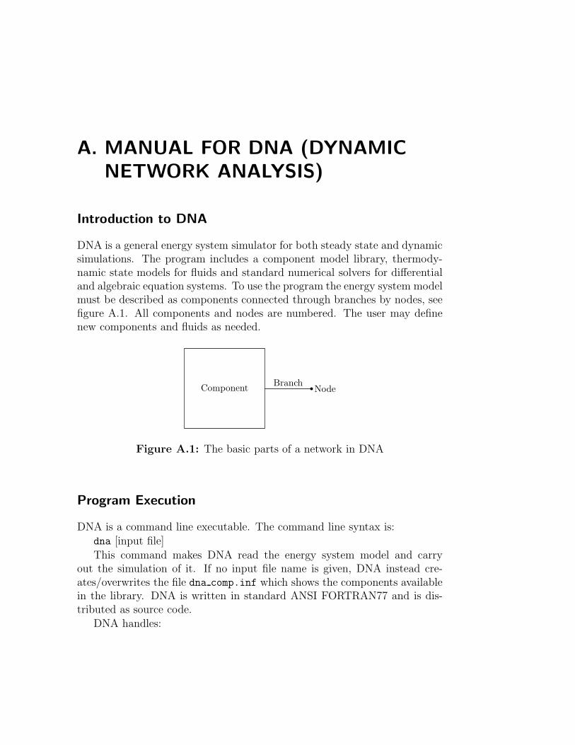
A. MANUAL FOR DNA (DYNAMICNETWORK ANALYSIS)
Introduction to DNA
DNA is a general energy system simulator for both steady state and dynamicsimulations. The program includes a component model library, thermody-namic state models for fluids and standard numerical solvers for differentialand algebraic equation systems. To use the program the energy system modelmust be described as components connected through branches by nodes, seefigure A.1. All components and nodes are numbered. The user may definenew components and fluids as needed.
Component BranchNode
Figure A.1: The basic parts of a network in DNA
Program Execution
DNA is a command line executable. The command line syntax is:
dna [input file]
This command makes DNA read the energy system model and carryout the simulation of it. If no input file name is given, DNA instead cre-ates/overwrites the file dna comp.inf which shows the components availablein the library. DNA is written in standard ANSI FORTRAN77 and is dis-tributed as source code.
DNA handles:
146 A. Manual for DNA (Dynamic Network Analysis)
• Steady-state and dynamic systems. Component parameters may beevaluated from a known operating point.
• variable fluid and solid flow compositions
• discontinuities in equations of dynamic systems
• generation of initial guesses for variables
• closed flow loops
An extensive check of the input is performed. DNA checks for errorswhich are reported on-screen and in a listing file. The check includes:
• syntax errors
• wrong component names
• connection of branches with different media
• missing initial values for differential variables
• missing additional conditions
• missing parameters
• missing fluid definitions
• multiple definitions of the same condition
DNA files
DNA uses the following files:
INPUT FILE (no file extension is presumed) The file that gives the neededinformation to simulate an energy system.
SIMULATION CONTROL FILE (this file’s extension is .dat) This fileholds information about handling of numerical routines, output controland more. If a file with the same name as the input file and extension.dat is present, it will be used. If it is not present the default filesimpar.dat will be used and a file with the same name as the inputfile and extension .dat is created and filled with data from simpar.dat.
147
LISTING FILE (this file’s extension is .lst) In this file any errors in theinput are presented. Errors are also presented on the standard output,but in case there are many errors this file is convenient. The listing fileis deleted if no error occurs.
STRUCTURE FILE (this file’s extension is .str) This file presents theinformation, DNA has gathered about the system during the setup ofa model. This file is intended for debugging of input.
VARIABLE ID FILE (This file’s extension is .id) This file is intendedto be used when the results of simulations should be transferred to aprogram that can show them graphically. The id-file shows all variablesthat are available from the simulation. By removing the * from a linein the file the user marks which variables are wanted as output fromthe prepare utility.
ASCII OUTPUT FILE (this file’s extension is .sta) This file presentsthe results of the simulation in a format readable by use of a texteditor.
MACHINE CODE OUTPUT FILE (this file’s extension is .dyn) Thisfile contains the results of a simulation in a format intended for readingby the utility prepare. With prepare this file is read and the variablesunmarked in the id-file are moved to tables in result files.
MEDIA OUTPUT FILE (This file’s extension is .med) If the machinecode output file is used this file is also created. It shows some additionalresults which are not included in the machine code output.
TABLE OUTPUT FILES (These files have extensions .f??, where thequestion marks indicate numbers) These files are output files from theprepare utility.
UPDATED INPUT FILE (This file’s extension is .upd) After a success-ful simulation a file similar to the input file but with updated initialguesses for variables is created. This file may be used as an inputfile to DNA. This file accesses an include file (.inc) which holds thepreviously found solution for all variables in the system.
COMPONENT LIBRARY FILE (the file is dna comp.inf) This file iscreated if no input file name is given in the call to DNA. The file viewsthe information available about the components in the component lib-rary.
148 A. Manual for DNA (Dynamic Network Analysis)
MODEL TEMPLATE (the file is template.dna) This file is a templatefor implementation of new component models in DNA.
Input File Syntax
A keyword approach is used for describing the system in the input file. Eachline starts with a main keyword. A line may consist of 80 characters in-cluding blanks which are dividing words, numbers and numerical values. Allkeywords may be given in either small or capital letters. Keyword length islimited to 20 characters.
TITLE A heading for each simulation may be given by this keyword. Thesyntax is:TITLE TC︷ ︸︸ ︷keyword
︷ ︸︸ ︷Title(string)
It may contain a maximum of 74 characters.
STRUC defines the system structure. The syntax is:STRUC [CN] NAME [V# . . . ] [N# . . . ] [P# . . . ]︷ ︸︸ ︷Keyword
︷ ︸︸ ︷Componentnumber(integer)
︷︸︸︷Type
︷ ︸︸ ︷Valuesfor eachvariableidentifier(integer)
︷ ︸︸ ︷Node
numbersfor eachbranch(integer)
︷ ︸︸ ︷Values foreach
parameter(real)
Only one component may be defined by each STRUC line. See the fileDna comp.inf for information about the component library. Compon-ent numbers must be positive and less than 1000. Node numbers mustbe positive and less than 100. A maximum of 100 components may bein a system. All system structure information may be seen in the .strfile. If the input line has to be longer than 80 characters, it may bedivided by a / at the end of each line.
MEDIA defines the flow medium in a given node. The syntax is:MEDIA [N# M# . . . ]︷ ︸︸ ︷Keyword
︷ ︸︸ ︷Sets ofnode andmediumnumber(integers)
An unlimited number of fluid definitions may follow MEDIA. Only onemedium definition is needed in each subsystem of a model. This maybe given by MEDIA, or it may be found in a component. The medium
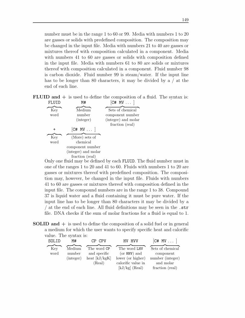
149
number must be in the range 1 to 60 or 99. Media with numbers 1 to 20are gasses or solids with predefined composition. The composition maybe changed in the input file. Media with numbers 21 to 40 are gasses ormixtures thereof with composition calculated in a component. Mediawith numbers 41 to 60 are gasses or solids with composition definedin the input file. Media with numbers 61 to 80 are solids or mixturesthereof with composition calculated in a component. Fluid number 98is carbon dioxide. Fluid number 99 is steam/water. If the input linehas to be longer than 80 characters, it may be divided by a / at theend of each line.
FLUID and + is used to define the composition of a fluid. The syntax is:FLUID M# [C# MV . . . ]︷ ︸︸ ︷Keyword
︷ ︸︸ ︷Mediumnumber(integer)
︷ ︸︸ ︷Sets of chemical
component number(integer) and molarfraction (real)
+ [C# MV . . . ]︷ ︸︸ ︷Keyword
︷ ︸︸ ︷(More) sets ofchemical
component number(integer) and molarfraction (real)
Only one fluid may be defined by each FLUID. The fluid number must inone of the ranges 1 to 20 and 41 to 60. Fluids with numbers 1 to 20 aregasses or mixtures thereof with predefined composition. The composi-tion may, however, be changed in the input file. Fluids with numbers41 to 60 are gasses or mixtures thereof with composition defined in theinput file. The compound numbers are in the range 1 to 38. Compound37 is liquid water and a fluid containing it must be pure water. If theinput line has to be longer than 80 characters it may be divided by a/ at the end of each line. All fluid definitions may be seen in the .strfile. DNA checks if the sum of molar fractions for a fluid is equal to 1.
SOLID and + is used to define the composition of a solid fuel or in generala medium for which the user wants to specify specific heat and calorificvalue. The syntax is:SOLID M# CP CPV HV HVV [C# MV . . . ]︷ ︸︸ ︷Keyword
︷ ︸︸ ︷Mediumnumber(integer)
︷ ︸︸ ︷The word CPand specificheat [kJ/kgK]
(Real)
︷ ︸︸ ︷The word LHV(or HHV) and
lower (or higher)calorific value in[kJ/kg] (Real)
︷ ︸︸ ︷Sets of chemicalcomponent
number (integer)and molar
fraction (real)
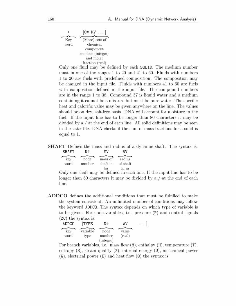
150 A. Manual for DNA (Dynamic Network Analysis)
+ [C# MV . . . ]︷ ︸︸ ︷Keyword
︷ ︸︸ ︷(More) sets ofchemicalcomponent
number (integer)and molar
fraction (real)Only one fluid may be defined by each SOLID. The medium numbermust in one of the ranges 1 to 20 and 41 to 60. Fluids with numbers1 to 20 are fuels with predefined composition. The composition maybe changed in the input file. Fluids with numbers 41 to 60 are fuelswith composition defined in the input file. The compound numbersare in the range 1 to 38. Compound 37 is liquid water and a mediumcontaining it cannot be a mixture but must be pure water. The specificheat and calorific value may be given anywhere on the line. The valuesshould be on dry, ash-free basis. DNA will account for moisture in thefuel. If the input line has to be longer than 80 characters it may bedivided by a / at the end of each line. All solid definitions may be seenin the .str file. DNA checks if the sum of mass fractions for a solid isequal to 1.
SHAFT Defines the mass and radius of a dynamic shaft. The syntax is:SHAFT N# MV RV︷ ︸︸ ︷keyword
︷ ︸︸ ︷nodenumber
︷ ︸︸ ︷mass ofshaft inkg
︷ ︸︸ ︷radiusof shaftin m
Only one shaft may be defined in each line. If the input line has to belonger than 80 characters it may be divided by a / at the end of eachline.
ADDCO defines the additional conditions that must be fulfilled to makethe system consistent. An unlimited number of conditions may followthe keyword ADDCO. The syntax depends on which type of variable isto be given. For node variables, i.e., pressure (P) and control signals(ZC) the syntax is:ADDCO [TYPE N# AV . . . ]︷ ︸︸ ︷keyword
︷ ︸︸ ︷variabletype
︷ ︸︸ ︷nodenumber(integer)
︷ ︸︸ ︷value(real)
For branch variables, i.e., mass flow (M), enthalpy (H), temperature (T),entropy (S), steam quality (X), internal energy (U), mechanical power(W), electrical power (E) and heat flow (Q) the syntax is:
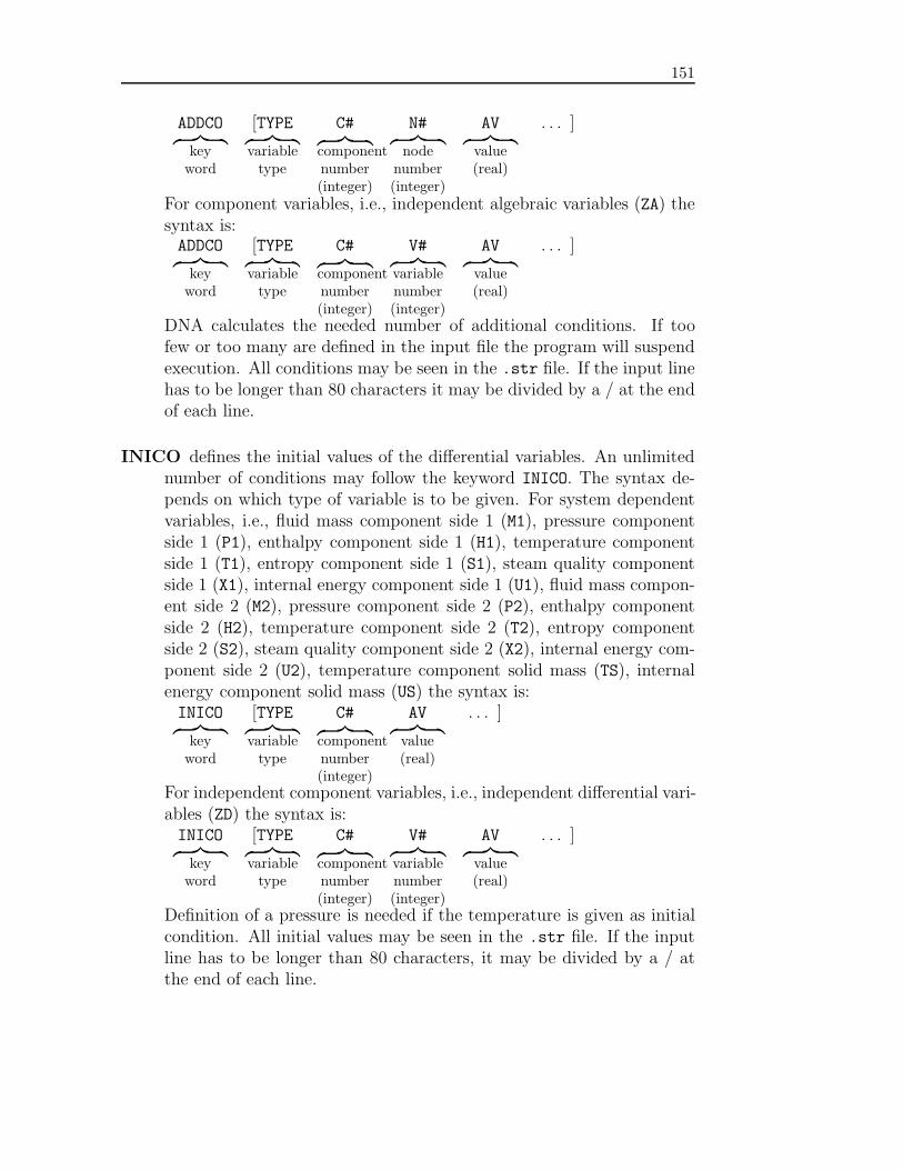
151
ADDCO [TYPE C# N# AV . . . ]︷ ︸︸ ︷keyword
︷ ︸︸ ︷variabletype
︷ ︸︸ ︷componentnumber(integer)
︷ ︸︸ ︷nodenumber(integer)
︷ ︸︸ ︷value(real)
For component variables, i.e., independent algebraic variables (ZA) thesyntax is:ADDCO [TYPE C# V# AV . . . ]︷ ︸︸ ︷keyword
︷ ︸︸ ︷variabletype
︷ ︸︸ ︷componentnumber(integer)
︷ ︸︸ ︷variablenumber(integer)
︷ ︸︸ ︷value(real)
DNA calculates the needed number of additional conditions. If toofew or too many are defined in the input file the program will suspendexecution. All conditions may be seen in the .str file. If the input linehas to be longer than 80 characters it may be divided by a / at the endof each line.
INICO defines the initial values of the differential variables. An unlimitednumber of conditions may follow the keyword INICO. The syntax de-pends on which type of variable is to be given. For system dependentvariables, i.e., fluid mass component side 1 (M1), pressure componentside 1 (P1), enthalpy component side 1 (H1), temperature componentside 1 (T1), entropy component side 1 (S1), steam quality componentside 1 (X1), internal energy component side 1 (U1), fluid mass compon-ent side 2 (M2), pressure component side 2 (P2), enthalpy componentside 2 (H2), temperature component side 2 (T2), entropy componentside 2 (S2), steam quality component side 2 (X2), internal energy com-ponent side 2 (U2), temperature component solid mass (TS), internalenergy component solid mass (US) the syntax is:INICO [TYPE C# AV . . . ]︷ ︸︸ ︷keyword
︷ ︸︸ ︷variabletype
︷ ︸︸ ︷componentnumber(integer)
︷ ︸︸ ︷value(real)
For independent component variables, i.e., independent differential vari-ables (ZD) the syntax is:INICO [TYPE C# V# AV . . . ]︷ ︸︸ ︷keyword
︷ ︸︸ ︷variabletype
︷ ︸︸ ︷componentnumber(integer)
︷ ︸︸ ︷variablenumber(integer)
︷ ︸︸ ︷value(real)
Definition of a pressure is needed if the temperature is given as initialcondition. All initial values may be seen in the .str file. If the inputline has to be longer than 80 characters, it may be divided by a / atthe end of each line.
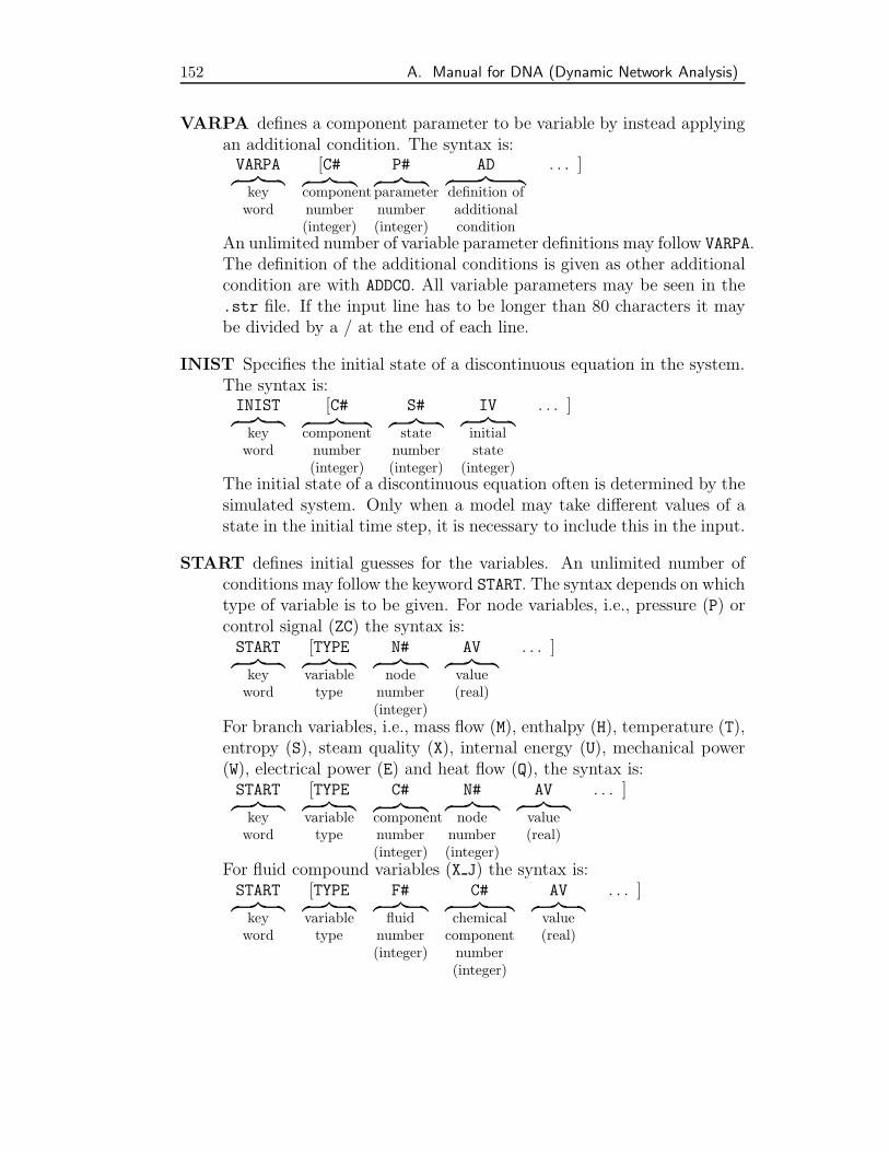
152 A. Manual for DNA (Dynamic Network Analysis)
VARPA defines a component parameter to be variable by instead applyingan additional condition. The syntax is:VARPA [C# P# AD . . . ]︷ ︸︸ ︷keyword
︷ ︸︸ ︷componentnumber(integer)
︷ ︸︸ ︷parameternumber(integer)
︷ ︸︸ ︷definition ofadditionalcondition
An unlimited number of variable parameter definitions may follow VARPA.The definition of the additional conditions is given as other additionalcondition are with ADDCO. All variable parameters may be seen in the.str file. If the input line has to be longer than 80 characters it maybe divided by a / at the end of each line.
INIST Specifies the initial state of a discontinuous equation in the system.The syntax is:INIST [C# S# IV . . . ]︷ ︸︸ ︷keyword
︷ ︸︸ ︷componentnumber(integer)
︷ ︸︸ ︷statenumber(integer)
︷ ︸︸ ︷initialstate
(integer)The initial state of a discontinuous equation often is determined by thesimulated system. Only when a model may take different values of astate in the initial time step, it is necessary to include this in the input.
START defines initial guesses for the variables. An unlimited number ofconditions may follow the keyword START. The syntax depends on whichtype of variable is to be given. For node variables, i.e., pressure (P) orcontrol signal (ZC) the syntax is:START [TYPE N# AV . . . ]︷ ︸︸ ︷keyword
︷ ︸︸ ︷variabletype
︷ ︸︸ ︷nodenumber(integer)
︷ ︸︸ ︷value(real)
For branch variables, i.e., mass flow (M), enthalpy (H), temperature (T),entropy (S), steam quality (X), internal energy (U), mechanical power(W), electrical power (E) and heat flow (Q), the syntax is:START [TYPE C# N# AV . . . ]︷ ︸︸ ︷keyword
︷ ︸︸ ︷variabletype
︷ ︸︸ ︷componentnumber(integer)
︷ ︸︸ ︷nodenumber(integer)
︷ ︸︸ ︷value(real)
For fluid compound variables (X J) the syntax is:START [TYPE F# C# AV . . . ]︷ ︸︸ ︷keyword
︷ ︸︸ ︷variabletype
︷ ︸︸ ︷fluid
number(integer)
︷ ︸︸ ︷chemicalcomponentnumber(integer)
︷ ︸︸ ︷value(real)
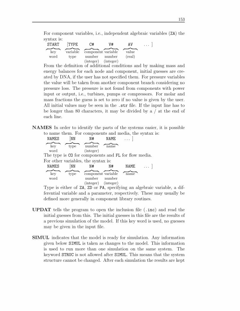
153
For component variables, i.e., independent algebraic variables (ZA) thesyntax is:START [TYPE C# V# AV . . . ]︷ ︸︸ ︷keyword
︷ ︸︸ ︷variabletype
︷ ︸︸ ︷componentnumber(integer)
︷ ︸︸ ︷variablenumber(integer)
︷ ︸︸ ︷value(real)
From the definition of additional conditions and by making mass andenergy balances for each node and component, initial guesses are cre-ated by DNA, if the user has not specified them. For pressure variablesthe value will be taken from another component branch considering nopressure loss. The pressure is not found from components with powerinput or output, i.e., turbines, pumps or compressors. For molar andmass fractions the guess is set to zero if no value is given by the user.All initial values may be seen in the .str file. If the input line has tobe longer than 80 characters, it may be divided by a / at the end ofeach line.
NAMES In order to identify the parts of the systems easier, it is possibleto name them. For components and media, the syntax is:NAMES [NN N# NAME . . . ]︷ ︸︸ ︷keyword
︷ ︸︸ ︷type
︷ ︸︸ ︷number(integer)
︷ ︸︸ ︷name
The type is CO for components and FL for flow media.For other variables, the syntax is:NAMES [NN N# N# NAME . . . ]︷ ︸︸ ︷keyword
︷ ︸︸ ︷type
︷ ︸︸ ︷componentnumber(integer)
︷ ︸︸ ︷variablenumber(integer)
︷ ︸︸ ︷name
Type is either of ZA, ZD or PA, specifying an algebraic variable, a dif-ferential variable and a parameter, respectively. These may usually bedefined more generally in component library routines.
UPDAT tells the program to open the inclusion file (.inc) and read theinitial guesses from this. The initial guesses in this file are the results ofa previous simulation of the model. If this key word is used, no guessesmay be given in the input file.
SIMUL indicates that the model is ready for simulation. Any informationgiven below SIMUL is taken as changes to the model. This informationis used to run more than one simulation on the same system. Thekeyword STRUC is not allowed after SIMUL. This means that the systemstructure cannot be changed. After each simulation the results are kept
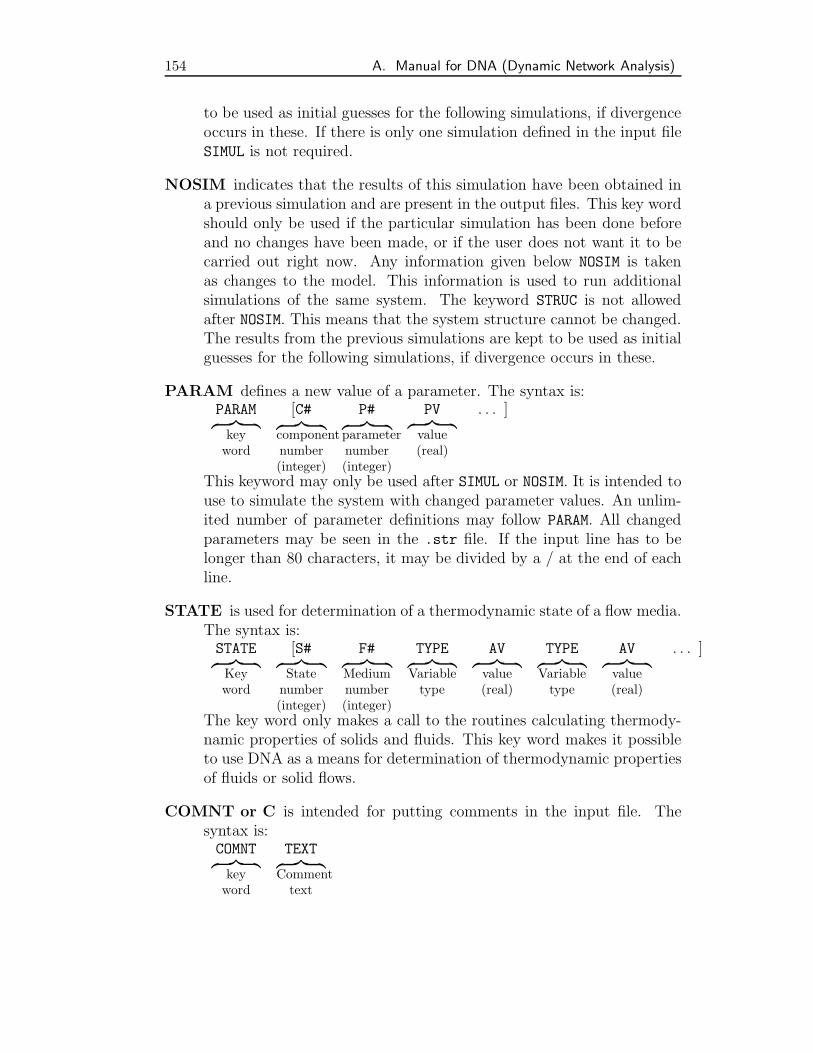
154 A. Manual for DNA (Dynamic Network Analysis)
to be used as initial guesses for the following simulations, if divergenceoccurs in these. If there is only one simulation defined in the input fileSIMUL is not required.
NOSIM indicates that the results of this simulation have been obtained ina previous simulation and are present in the output files. This key wordshould only be used if the particular simulation has been done beforeand no changes have been made, or if the user does not want it to becarried out right now. Any information given below NOSIM is takenas changes to the model. This information is used to run additionalsimulations of the same system. The keyword STRUC is not allowedafter NOSIM. This means that the system structure cannot be changed.The results from the previous simulations are kept to be used as initialguesses for the following simulations, if divergence occurs in these.
PARAM defines a new value of a parameter. The syntax is:PARAM [C# P# PV . . . ]︷ ︸︸ ︷keyword
︷ ︸︸ ︷componentnumber(integer)
︷ ︸︸ ︷parameternumber(integer)
︷ ︸︸ ︷value(real)
This keyword may only be used after SIMUL or NOSIM. It is intended touse to simulate the system with changed parameter values. An unlim-ited number of parameter definitions may follow PARAM. All changedparameters may be seen in the .str file. If the input line has to belonger than 80 characters, it may be divided by a / at the end of eachline.
STATE is used for determination of a thermodynamic state of a flow media.The syntax is:STATE [S# F# TYPE AV TYPE AV . . . ]︷ ︸︸ ︷Keyword
︷ ︸︸ ︷Statenumber(integer)
︷ ︸︸ ︷Mediumnumber(integer)
︷ ︸︸ ︷Variabletype
︷ ︸︸ ︷value(real)
︷ ︸︸ ︷Variabletype
︷ ︸︸ ︷value(real)
The key word only makes a call to the routines calculating thermody-namic properties of solids and fluids. This key word makes it possibleto use DNA as a means for determination of thermodynamic propertiesof fluids or solid flows.
COMNT or C is intended for putting comments in the input file. Thesyntax is:COMNT TEXT︷ ︸︸ ︷keyword
︷ ︸︸ ︷Commenttext

155
orC TEXT︷ ︸︸ ︷keyword
︷ ︸︸ ︷Commenttext
If the input line has to be longer than 80 characters, it may be dividedby a / at the end of each line.
is intended for encapsulating parts of the input file and thereby exclud-ing them from being read by DNA. This is handy for debugging if asimulation does not converge and the user does not want to remove thealready written text. The syntax is:
TEXT . . .︷ ︸︸ ︷delimiter
︷ ︸︸ ︷Commenttext
. . . ︷ ︸︸ ︷moretext
︷ ︸︸ ︷delimiter
and may be put anywhere on a line, and may span over multiplelines.
Media
To formulate a model, the medium in each node has to be known. Thesedefinitions should be done in the component routines, or by the MEDIA keyword, depending on the component model.
The available media are identified by numbers. They may be divided intogroups:
Numbers 1–20 Flow media with pre-defined composition specified in theDNA source code. The definitions may be overwritten but numbers 41–60 and 61–80 should preferably be used instead for fluids and solids,respectively.
Numbers 21–40 Flow media with composition calculated in a componentduring simulation. The composition may be calculated ahead of thesolution or be included in the equations and solved. The former methodshould be used with care, because the composition will be calculatedbased on the initial guesses for the variables in the system.
Numbers 41-60 Fluid media with composition specified in the input file tothe program. These are defined with the key word FLUID.
Numbers 61-80 Solid media with composition specified in the input file tothe program. These are defined with the key word SOLID.
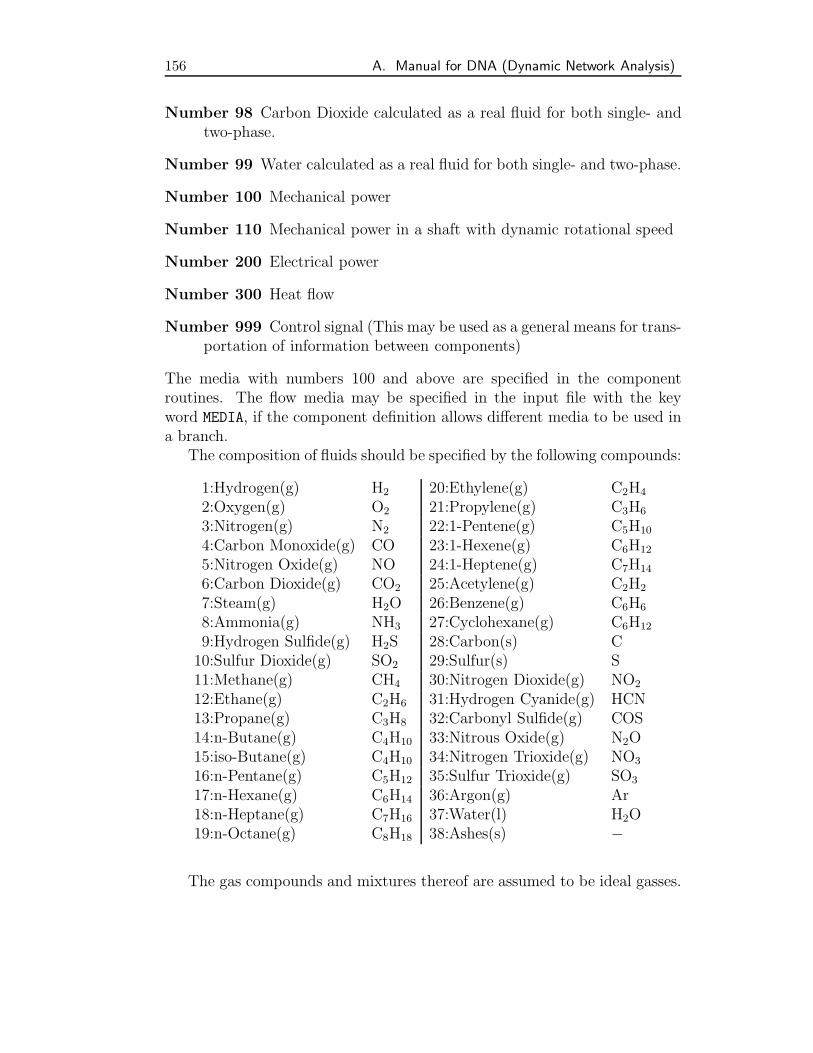
156 A. Manual for DNA (Dynamic Network Analysis)
Number 98 Carbon Dioxide calculated as a real fluid for both single- andtwo-phase.
Number 99 Water calculated as a real fluid for both single- and two-phase.
Number 100 Mechanical power
Number 110 Mechanical power in a shaft with dynamic rotational speed
Number 200 Electrical power
Number 300 Heat flow
Number 999 Control signal (This may be used as a general means for trans-portation of information between components)
The media with numbers 100 and above are specified in the componentroutines. The flow media may be specified in the input file with the keyword MEDIA, if the component definition allows different media to be used ina branch.
The composition of fluids should be specified by the following compounds:
1:Hydrogen(g) H2 20:Ethylene(g) C2H4
2:Oxygen(g) O2 21:Propylene(g) C3H6
3:Nitrogen(g) N2 22:1-Pentene(g) C5H10
4:Carbon Monoxide(g) CO 23:1-Hexene(g) C6H12
5:Nitrogen Oxide(g) NO 24:1-Heptene(g) C7H14
6:Carbon Dioxide(g) CO2 25:Acetylene(g) C2H2
7:Steam(g) H2O 26:Benzene(g) C6H6
8:Ammonia(g) NH3 27:Cyclohexane(g) C6H12
9:Hydrogen Sulfide(g) H2S 28:Carbon(s) C10:Sulfur Dioxide(g) SO2 29:Sulfur(s) S11:Methane(g) CH4 30:Nitrogen Dioxide(g) NO2
12:Ethane(g) C2H6 31:Hydrogen Cyanide(g) HCN13:Propane(g) C3H8 32:Carbonyl Sulfide(g) COS14:n-Butane(g) C4H10 33:Nitrous Oxide(g) N2O15:iso-Butane(g) C4H10 34:Nitrogen Trioxide(g) NO3
16:n-Pentane(g) C5H12 35:Sulfur Trioxide(g) SO3
17:n-Hexane(g) C6H14 36:Argon(g) Ar18:n-Heptane(g) C7H16 37:Water(l) H2O19:n-Octane(g) C8H18 38:Ashes(s) −
The gas compounds and mixtures thereof are assumed to be ideal gasses.
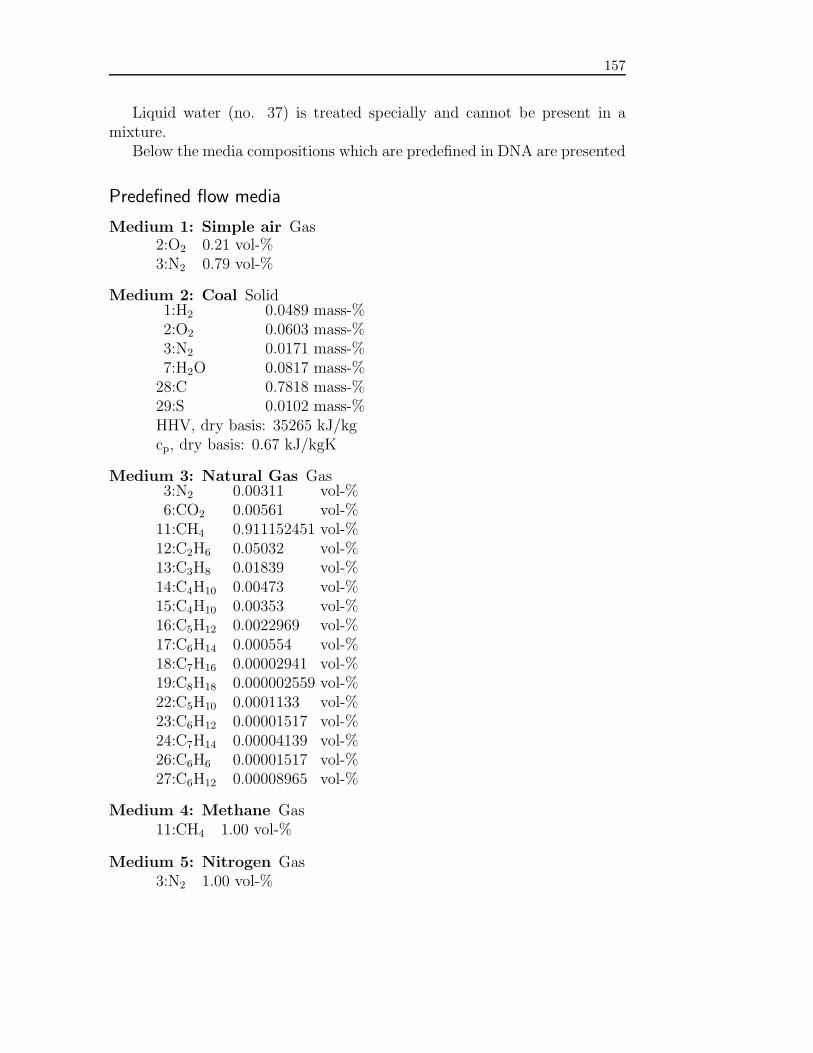
157
Liquid water (no. 37) is treated specially and cannot be present in amixture.
Below the media compositions which are predefined in DNA are presented
Predefined flow media
Medium 1: Simple air Gas2:O2 0.21 vol-%3:N2 0.79 vol-%
Medium 2: Coal Solid1:H2 0.0489 mass-%2:O2 0.0603 mass-%3:N2 0.0171 mass-%7:H2O 0.0817 mass-%28:C 0.7818 mass-%29:S 0.0102 mass-%HHV, dry basis: 35265 kJ/kgcp, dry basis: 0.67 kJ/kgK
Medium 3: Natural Gas Gas3:N2 0.00311 vol-%6:CO2 0.00561 vol-%11:CH4 0.911152451 vol-%12:C2H6 0.05032 vol-%13:C3H8 0.01839 vol-%14:C4H10 0.00473 vol-%15:C4H10 0.00353 vol-%16:C5H12 0.0022969 vol-%17:C6H14 0.000554 vol-%18:C7H16 0.00002941 vol-%19:C8H18 0.000002559 vol-%22:C5H10 0.0001133 vol-%23:C6H12 0.00001517 vol-%24:C7H14 0.00004139 vol-%26:C6H6 0.00001517 vol-%27:C6H12 0.00008965 vol-%
Medium 4: Methane Gas11:CH4 1.00 vol-%
Medium 5: Nitrogen Gas3:N2 1.00 vol-%
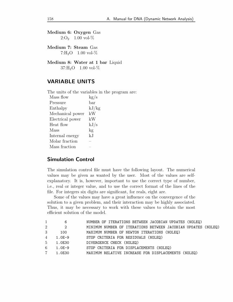
158 A. Manual for DNA (Dynamic Network Analysis)
Medium 6: Oxygen Gas2:O2 1.00 vol-%
Medium 7: Steam Gas7:H2O 1.00 vol-%
Medium 8: Water at 1 bar Liquid37:H2O 1.00 vol-%
VARIABLE UNITS
The units of the variables in the program are:Mass flow kg/sPressure barEnthalpy kJ/kgMechanical power kWElectrical power kWHeat flow kJ/sMass kgInternal energy kJMolar fraction –Mass fraction –
Simulation Control
The simulation control file must have the following layout. The numericalvalues may be given as wanted by the user. Most of the values are self-explanatory. It is, however, important to use the correct type of number,i.e., real or integer value, and to use the correct format of the lines of thefile. For integers six digits are significant, for reals, eight are.
Some of the values may have a great influence on the convergence of thesolution to a given problem, and their interaction may be highly associated.Thus, it may be necessary to work with these values to obtain the mostefficient solution of the model.
1 6 NUMBER OF ITERATIONS BETWEEN JACOBIAN UPDATES (NOLEQ)2 2 MINIMUM NUMBER OF ITERATIONS BETWEEN JACOBIAN UPDATES (NOLEQ)3 100 MAXIMUM NUMBER OF NEWTON ITERATIONS (NOLEQ)4 1.0E-9 STOP CRITERIA FOR RESIDUALS (NOLEQ)5 1.0E30 DIVERGENCE CHECK (NOLEQ)6 1.0E-9 STOP CRITERIA FOR DISPLACEMENTS (NOLEQ)7 1.0E30 MAXIMUM RELATIVE INCREASE FOR DISPLACEMENTS (NOLEQ)
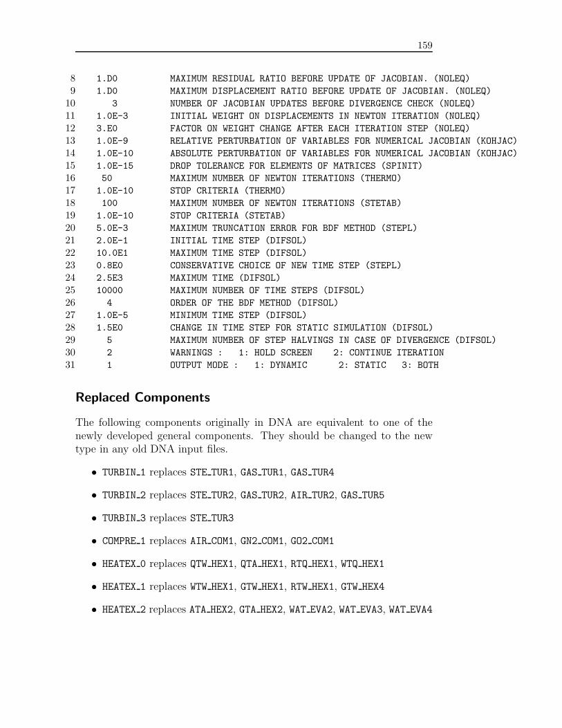
159
8 1.D0 MAXIMUM RESIDUAL RATIO BEFORE UPDATE OF JACOBIAN. (NOLEQ)9 1.D0 MAXIMUM DISPLACEMENT RATIO BEFORE UPDATE OF JACOBIAN. (NOLEQ)10 3 NUMBER OF JACOBIAN UPDATES BEFORE DIVERGENCE CHECK (NOLEQ)11 1.0E-3 INITIAL WEIGHT ON DISPLACEMENTS IN NEWTON ITERATION (NOLEQ)12 3.E0 FACTOR ON WEIGHT CHANGE AFTER EACH ITERATION STEP (NOLEQ)13 1.0E-9 RELATIVE PERTURBATION OF VARIABLES FOR NUMERICAL JACOBIAN (KOHJAC)14 1.0E-10 ABSOLUTE PERTURBATION OF VARIABLES FOR NUMERICAL JACOBIAN (KOHJAC)15 1.0E-15 DROP TOLERANCE FOR ELEMENTS OF MATRICES (SPINIT)16 50 MAXIMUM NUMBER OF NEWTON ITERATIONS (THERMO)17 1.0E-10 STOP CRITERIA (THERMO)18 100 MAXIMUM NUMBER OF NEWTON ITERATIONS (STETAB)19 1.0E-10 STOP CRITERIA (STETAB)20 5.0E-3 MAXIMUM TRUNCATION ERROR FOR BDF METHOD (STEPL)21 2.0E-1 INITIAL TIME STEP (DIFSOL)22 10.0E1 MAXIMUM TIME STEP (DIFSOL)23 0.8E0 CONSERVATIVE CHOICE OF NEW TIME STEP (STEPL)24 2.5E3 MAXIMUM TIME (DIFSOL)25 10000 MAXIMUM NUMBER OF TIME STEPS (DIFSOL)26 4 ORDER OF THE BDF METHOD (DIFSOL)27 1.0E-5 MINIMUM TIME STEP (DIFSOL)28 1.5E0 CHANGE IN TIME STEP FOR STATIC SIMULATION (DIFSOL)29 5 MAXIMUM NUMBER OF STEP HALVINGS IN CASE OF DIVERGENCE (DIFSOL)30 2 WARNINGS : 1: HOLD SCREEN 2: CONTINUE ITERATION31 1 OUTPUT MODE : 1: DYNAMIC 2: STATIC 3: BOTH
Replaced Components
The following components originally in DNA are equivalent to one of thenewly developed general components. They should be changed to the newtype in any old DNA input files.
• TURBIN 1 replaces STE TUR1, GAS TUR1, GAS TUR4
• TURBIN 2 replaces STE TUR2, GAS TUR2, AIR TUR2, GAS TUR5
• TURBIN 3 replaces STE TUR3
• COMPRE 1 replaces AIR COM1, GN2 COM1, GO2 COM1
• HEATEX 0 replaces QTW HEX1, QTA HEX1, RTQ HEX1, WTQ HEX1
• HEATEX 1 replaces WTW HEX1, GTW HEX1, RTW HEX1, GTW HEX4
• HEATEX 2 replaces ATA HEX2, GTA HEX2, WAT EVA2, WAT EVA3, WAT EVA4
160 A. Manual for DNA (Dynamic Network Analysis)
• HEATEX 3 replaces WTW HEX3, GTW HEX3, WTA HEX3, GTW HEX6
• HEATEX 7 replaces ATA HEX7
• VALVE 01 replaces WAT VAL1, SYN VAL1
• SPLITTER replaces WAT SPLI, AIR SPLI, GAS SPLC, GAS SPLV
• MIXER 01 replaces AN2 MIX1
• ADDANODE replaces WAT HELP
• LIQPUM 1 replaces WAT PUM1
• LIQSEP 1 replaces WAT SEP1
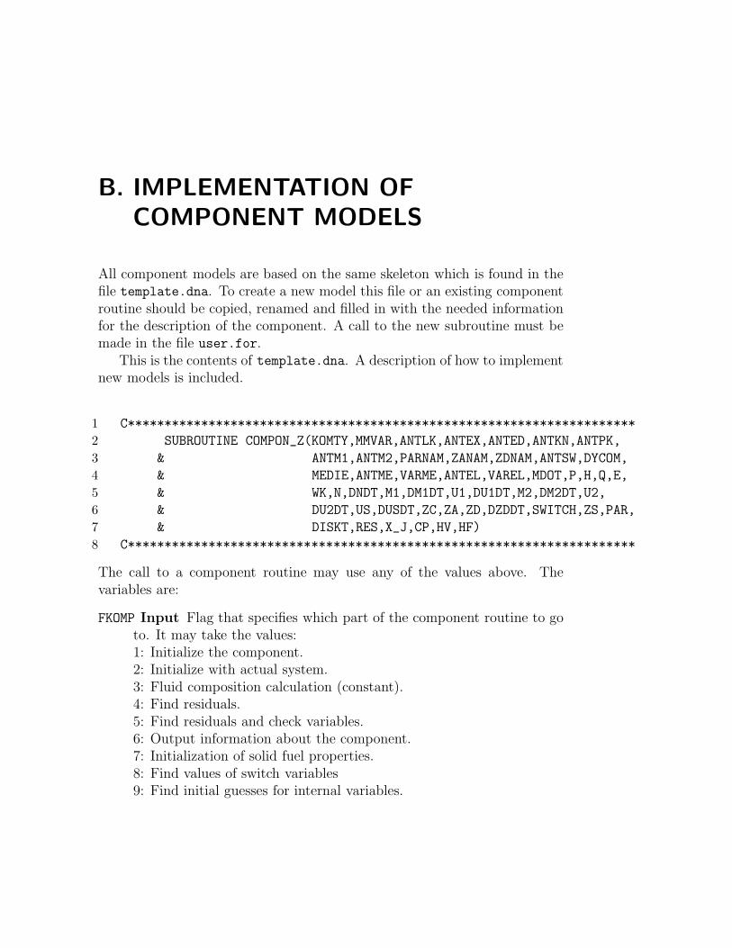
B. IMPLEMENTATION OFCOMPONENT MODELS
All component models are based on the same skeleton which is found in thefile template.dna. To create a new model this file or an existing componentroutine should be copied, renamed and filled in with the needed informationfor the description of the component. A call to the new subroutine must bemade in the file user.for.
This is the contents of template.dna. A description of how to implementnew models is included.
1 C*********************************************************************
2 SUBROUTINE COMPON_Z(KOMTY,MMVAR,ANTLK,ANTEX,ANTED,ANTKN,ANTPK,
3 & ANTM1,ANTM2,PARNAM,ZANAM,ZDNAM,ANTSW,DYCOM,
4 & MEDIE,ANTME,VARME,ANTEL,VAREL,MDOT,P,H,Q,E,
5 & WK,N,DNDT,M1,DM1DT,U1,DU1DT,M2,DM2DT,U2,
6 & DU2DT,US,DUSDT,ZC,ZA,ZD,DZDDT,SWITCH,ZS,PAR,
7 & DISKT,RES,X_J,CP,HV,HF)
8 C*********************************************************************
The call to a component routine may use any of the values above. Thevariables are:
FKOMP Input Flag that specifies which part of the component routine to goto. It may take the values:1: Initialize the component.2: Initialize with actual system.3: Fluid composition calculation (constant).4: Find residuals.5: Find residuals and check variables.6: Output information about the component.7: Initialization of solid fuel properties.8: Find values of switch variables9: Find initial guesses for internal variables.
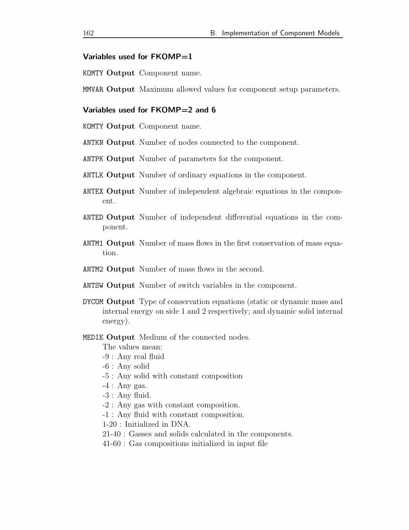
162 B. Implementation of Component Models
Variables used for FKOMP=1
KOMTY Output Component name.
MMVAR Output Maximum allowed values for component setup parameters.
Variables used for FKOMP=2 and 6
KOMTY Output Component name.
ANTKN Output Number of nodes connected to the component.
ANTPK Output Number of parameters for the component.
ANTLK Output Number of ordinary equations in the component.
ANTEX Output Number of independent algebraic equations in the compon-ent.
ANTED Output Number of independent differential equations in the com-ponent.
ANTM1 Output Number of mass flows in the first conservation of mass equa-tion.
ANTM2 Output Number of mass flows in the second.
ANTSW Output Number of switch variables in the component.
DYCOM Output Type of conservation equations (static or dynamic mass andinternal energy on side 1 and 2 respectively; and dynamic solid internalenergy).
MEDIE Output Medium of the connected nodes.The values mean:-9 : Any real fluid-6 : Any solid-5 : Any solid with constant composition-4 : Any gas.-3 : Any fluid.-2 : Any gas with constant composition.-1 : Any fluid with constant composition.1-20 : Initialized in DNA.21-40 : Gasses and solids calculated in the components.41-60 : Gas compositions initialized in input file
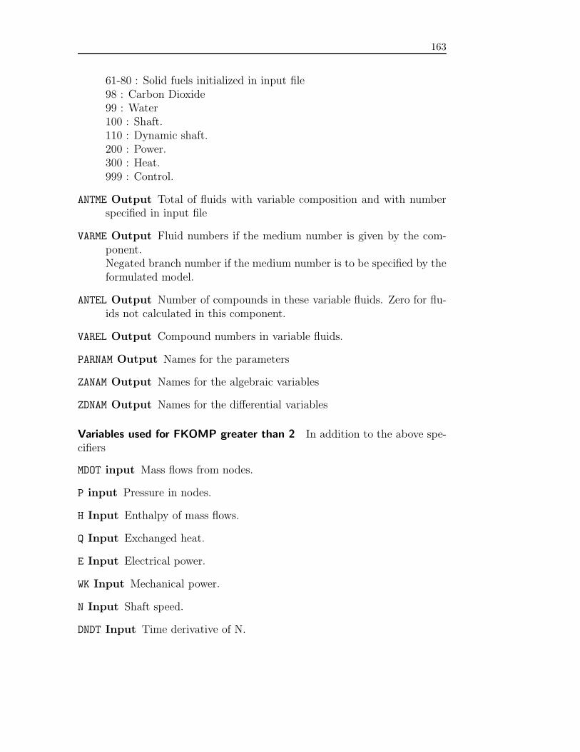
163
61-80 : Solid fuels initialized in input file98 : Carbon Dioxide99 : Water100 : Shaft.110 : Dynamic shaft.200 : Power.300 : Heat.999 : Control.
ANTME Output Total of fluids with variable composition and with numberspecified in input file
VARME Output Fluid numbers if the medium number is given by the com-ponent.Negated branch number if the medium number is to be specified by theformulated model.
ANTEL Output Number of compounds in these variable fluids. Zero for flu-ids not calculated in this component.
VAREL Output Compound numbers in variable fluids.
PARNAM Output Names for the parameters
ZANAM Output Names for the algebraic variables
ZDNAM Output Names for the differential variables
Variables used for FKOMP greater than 2 In addition to the above spe-cifiers
MDOT input Mass flows from nodes.
P input Pressure in nodes.
H Input Enthalpy of mass flows.
Q Input Exchanged heat.
E Input Electrical power.
WK Input Mechanical power.
N Input Shaft speed.
DNDT Input Time derivative of N.
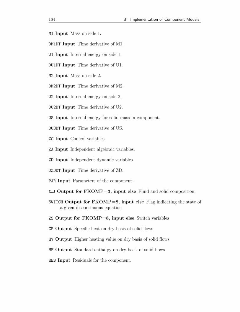
164 B. Implementation of Component Models
M1 Input Mass on side 1.
DM1DT Input Time derivative of M1.
U1 Input Internal energy on side 1.
DU1DT Input Time derivative of U1.
M2 Input Mass on side 2.
DM2DT Input Time derivative of M2.
U2 Input Internal energy on side 2.
DU2DT Input Time derivative of U2.
US Input Internal energy for solid mass in component.
DUSDT Input Time derivative of US.
ZC Input Control variables.
ZA Input Independent algebraic variables.
ZD Input Independent dynamic variables.
DZDDT Input Time derivative of ZD.
PAR Input Parameters of the component.
X J Output for FKOMP=3, input else Fluid and solid composition.
SWITCH Output for FKOMP=8, input else Flag indicating the state ofa given discontinuous equation
ZS Output for FKOMP=8, input else Switch variables
CP Output Specific heat on dry basis of solid flows
HV Output Higher heating value on dry basis of solid flows
HF Output Standard enthalpy on dry basis of solid flows
RES Input Residuals for the component.

165
Local variables used for FKOMP=6
K PAR Parameter description.
K LIG Equation description.
K BET Condition description.
K MED Media description.
Subroutines for use in component routines
STATES Thermodynamic properties of flows.The call syntax is:CALL STATES(P,H,T,V,S,X,U,ID1,ID2,MEDIE)P :Pressure [bar]H :Specific enthalpy [kJ/kg]T :Temperature [C ]V :Specific volume [m3/kg]S :Specific entropy [kJ/kgK]X :Steam quality [–] (For real fluids only)U :Specific internal energy [kJ/kg]ID1 :Identifier for input parameterID2 :Identifier for input parameterMEDIE:Medium numberThe routine calculates the remaining values from the two given prop-erties.
GASVIS Transport properties of fluids.The call syntax is:CALL TRAPRO(VISCOS,CONDUC,PRNDTL,P,T,V,X J,MEDIE,FLAG)VISCOS:Viscosity [Ns/m2]CONDUC:Thermal conductivity [W/mK]PRNDTL:Prandtl number [–]P :Pressure [bar]T :Temperature [C ]V :Specific volume [m3/kg]X J :Fluid composition arrayFLAG :Flag indicating if thermal conductivity is to be calculated
.
Viscosity, thermal conductivity and Prandtl number of a fluid is calcu-lated as a function of pressure, temperature and specific volume.
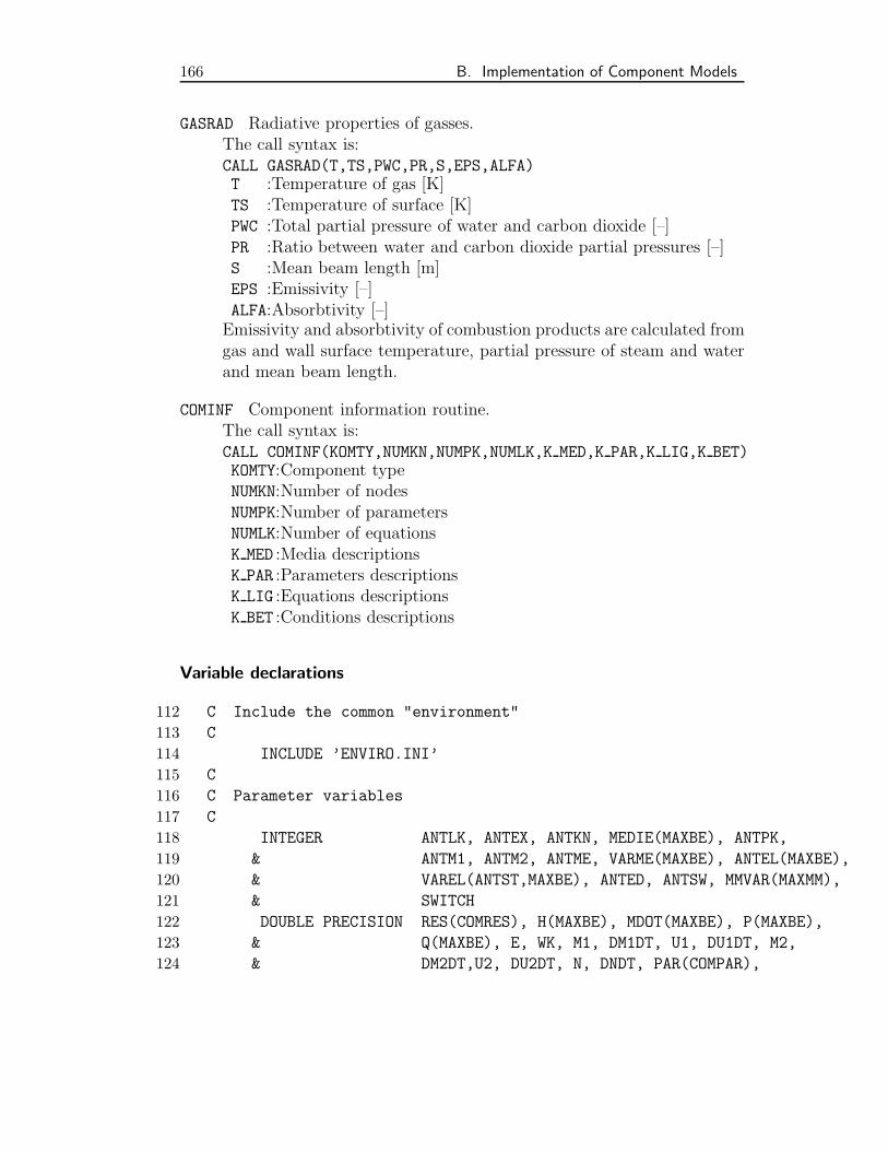
166 B. Implementation of Component Models
GASRAD Radiative properties of gasses.The call syntax is:CALL GASRAD(T,TS,PWC,PR,S,EPS,ALFA)T :Temperature of gas [K]TS :Temperature of surface [K]PWC :Total partial pressure of water and carbon dioxide [–]PR :Ratio between water and carbon dioxide partial pressures [–]S :Mean beam length [m]EPS :Emissivity [–]ALFA:Absorbtivity [–]Emissivity and absorbtivity of combustion products are calculated fromgas and wall surface temperature, partial pressure of steam and waterand mean beam length.
COMINF Component information routine.The call syntax is:CALL COMINF(KOMTY,NUMKN,NUMPK,NUMLK,K MED,K PAR,K LIG,K BET)KOMTY:Component typeNUMKN:Number of nodesNUMPK:Number of parametersNUMLK:Number of equationsK MED :Media descriptionsK PAR :Parameters descriptionsK LIG :Equations descriptionsK BET :Conditions descriptions
Variable declarations
112 C Include the common "environment"
113 C
114 INCLUDE ’ENVIRO.INI’
115 C
116 C Parameter variables
117 C
118 INTEGER ANTLK, ANTEX, ANTKN, MEDIE(MAXBE), ANTPK,
119 & ANTM1, ANTM2, ANTME, VARME(MAXBE), ANTEL(MAXBE),
120 & VAREL(ANTST,MAXBE), ANTED, ANTSW, MMVAR(MAXMM),
121 & SWITCH
122 DOUBLE PRECISION RES(COMRES), H(MAXBE), MDOT(MAXBE), P(MAXBE),
123 & Q(MAXBE), E, WK, M1, DM1DT, U1, DU1DT, M2,
124 & DM2DT,U2, DU2DT, N, DNDT, PAR(COMPAR),
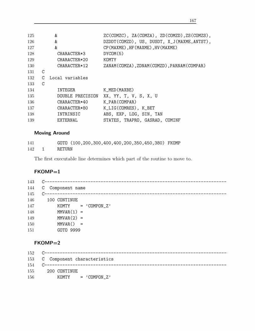
167
125 & ZC(COMZC), ZA(COMZA), ZD(COMZD),ZS(COMZS),
126 & DZDDT(COMZD), US, DUSDT, X_J(MAXME,ANTST),
127 & CP(MAXME),HF(MAXME),HV(MAXME)
128 CHARACTER*3 DYCOM(5)
129 CHARACTER*20 KOMTY
130 CHARACTER*12 ZANAM(COMZA),ZDNAM(COMZD),PARNAM(COMPAR)
131 C
132 C Local variables
133 C
134 INTEGER K_MED(MAXBE)
135 DOUBLE PRECISION XX, YY, T, V, S, X, U
136 CHARACTER*40 K_PAR(COMPAR)
137 CHARACTER*80 K_LIG(COMRES), K_BET
138 INTRINSIC ABS, EXP, LOG, SIN, TAN
139 EXTERNAL STATES, TRAPRO, GASRAD, COMINF
Moving Around
141 GOTO (100,200,300,400,400,200,350,450,380) FKOMP
142 1 RETURN
The first executable line determines which part of the routine to move to.
FKOMP=1
143 C-----------------------------------------------------------------------
144 C Component name
145 C-----------------------------------------------------------------------
146 100 CONTINUE
147 KOMTY = ’COMPON_Z’
148 MMVAR(1) =
149 MMVAR(2) =
150 MMVAR() =
151 GOTO 9999
FKOMP=2
152 C-----------------------------------------------------------------------
153 C Component characteristics
154 C-----------------------------------------------------------------------
155 200 CONTINUE
156 KOMTY = ’COMPON_Z’
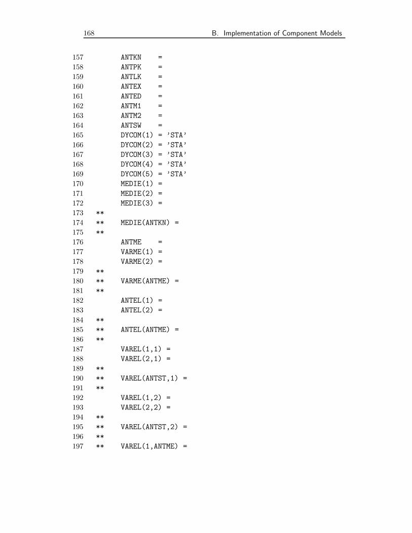
168 B. Implementation of Component Models
157 ANTKN =
158 ANTPK =
159 ANTLK =
160 ANTEX =
161 ANTED =
162 ANTM1 =
163 ANTM2 =
164 ANTSW =
165 DYCOM(1) = ’STA’
166 DYCOM(2) = ’STA’
167 DYCOM(3) = ’STA’
168 DYCOM(4) = ’STA’
169 DYCOM(5) = ’STA’
170 MEDIE(1) =
171 MEDIE(2) =
172 MEDIE(3) =
173 **
174 ** MEDIE(ANTKN) =
175 **
176 ANTME =
177 VARME(1) =
178 VARME(2) =
179 **
180 ** VARME(ANTME) =
181 **
182 ANTEL(1) =
183 ANTEL(2) =
184 **
185 ** ANTEL(ANTME) =
186 **
187 VAREL(1,1) =
188 VAREL(2,1) =
189 **
190 ** VAREL(ANTST,1) =
191 **
192 VAREL(1,2) =
193 VAREL(2,2) =
194 **
195 ** VAREL(ANTST,2) =
196 **
197 ** VAREL(1,ANTME) =
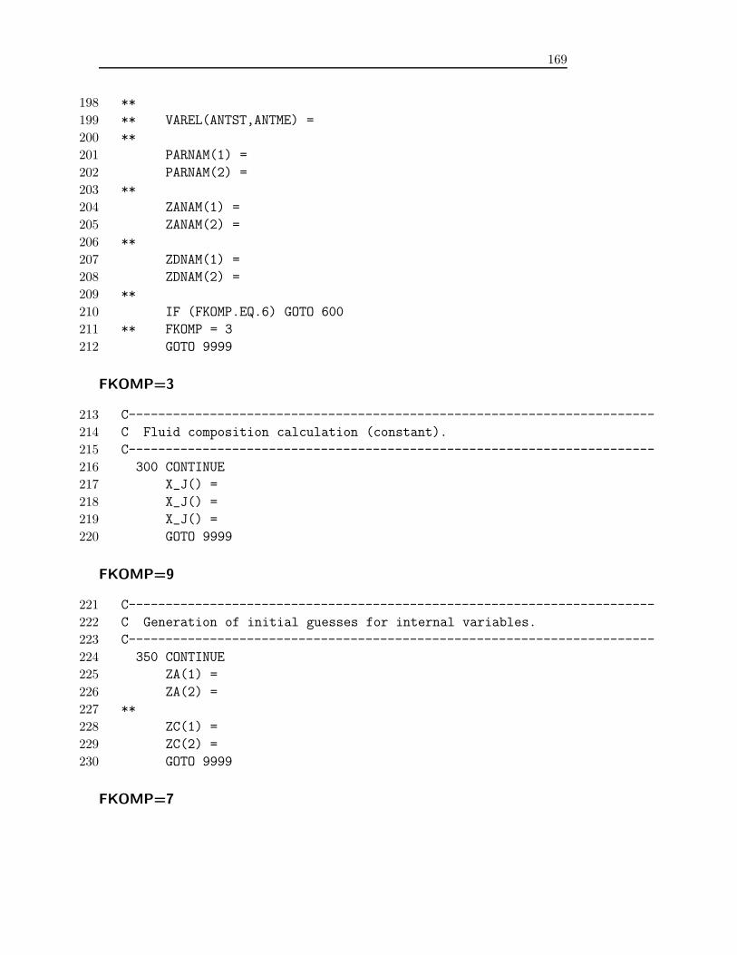
169
198 **
199 ** VAREL(ANTST,ANTME) =
200 **
201 PARNAM(1) =
202 PARNAM(2) =
203 **
204 ZANAM(1) =
205 ZANAM(2) =
206 **
207 ZDNAM(1) =
208 ZDNAM(2) =
209 **
210 IF (FKOMP.EQ.6) GOTO 600
211 ** FKOMP = 3
212 GOTO 9999
FKOMP=3
213 C-----------------------------------------------------------------------
214 C Fluid composition calculation (constant).
215 C-----------------------------------------------------------------------
216 300 CONTINUE
217 X_J() =
218 X_J() =
219 X_J() =
220 GOTO 9999
FKOMP=9
221 C-----------------------------------------------------------------------
222 C Generation of initial guesses for internal variables.
223 C-----------------------------------------------------------------------
224 350 CONTINUE
225 ZA(1) =
226 ZA(2) =
227 **
228 ZC(1) =
229 ZC(2) =
230 GOTO 9999
FKOMP=7
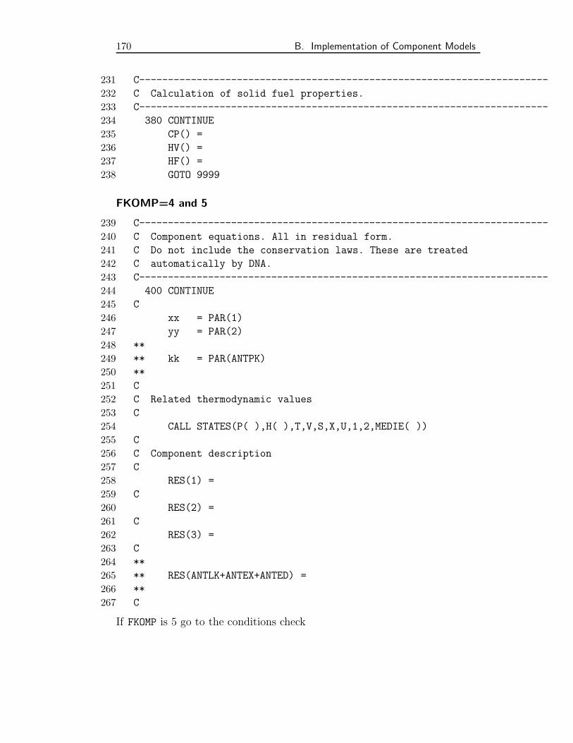
170 B. Implementation of Component Models
231 C-----------------------------------------------------------------------
232 C Calculation of solid fuel properties.
233 C-----------------------------------------------------------------------
234 380 CONTINUE
235 CP() =
236 HV() =
237 HF() =
238 GOTO 9999
FKOMP=4 and 5
239 C-----------------------------------------------------------------------
240 C Component equations. All in residual form.
241 C Do not include the conservation laws. These are treated
242 C automatically by DNA.
243 C-----------------------------------------------------------------------
244 400 CONTINUE
245 C
246 xx = PAR(1)
247 yy = PAR(2)
248 **
249 ** kk = PAR(ANTPK)
250 **
251 C
252 C Related thermodynamic values
253 C
254 CALL STATES(P( ),H( ),T,V,S,X,U,1,2,MEDIE( ))
255 C
256 C Component description
257 C
258 RES(1) =
259 C
260 RES(2) =
261 C
262 RES(3) =
263 C
264 **
265 ** RES(ANTLK+ANTEX+ANTED) =
266 **
267 C
If FKOMP is 5 go to the conditions check
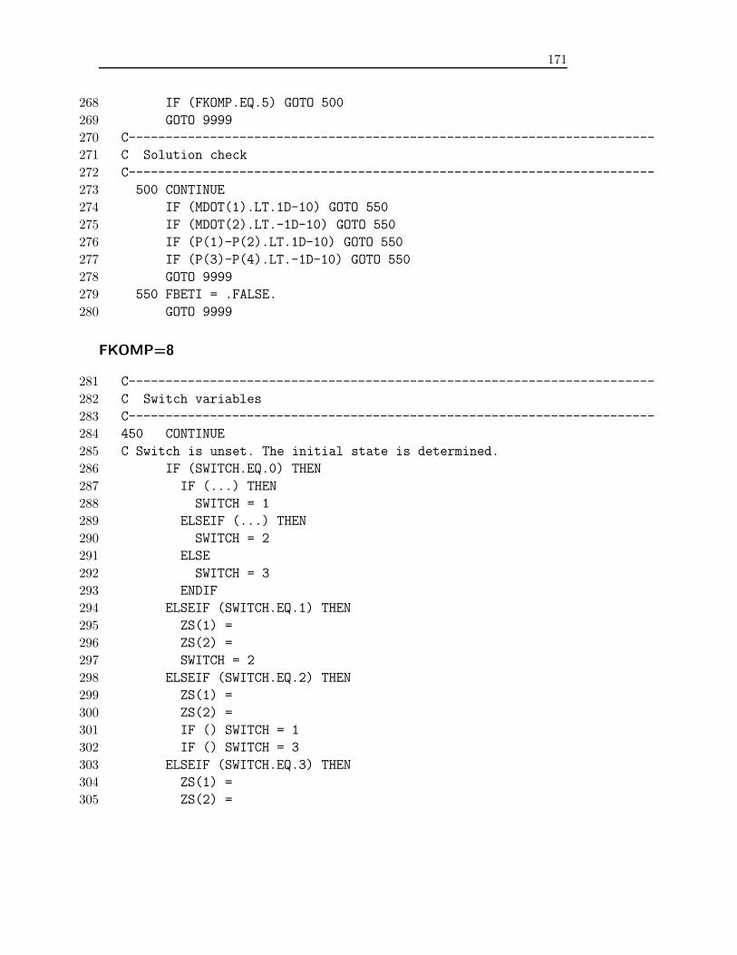
171
268 IF (FKOMP.EQ.5) GOTO 500
269 GOTO 9999
270 C-----------------------------------------------------------------------
271 C Solution check
272 C-----------------------------------------------------------------------
273 500 CONTINUE
274 IF (MDOT(1).LT.1D-10) GOTO 550
275 IF (MDOT(2).LT.-1D-10) GOTO 550
276 IF (P(1)-P(2).LT.1D-10) GOTO 550
277 IF (P(3)-P(4).LT.-1D-10) GOTO 550
278 GOTO 9999
279 550 FBETI = .FALSE.
280 GOTO 9999
FKOMP=8
281 C-----------------------------------------------------------------------
282 C Switch variables
283 C-----------------------------------------------------------------------
284 450 CONTINUE
285 C Switch is unset. The initial state is determined.
286 IF (SWITCH.EQ.0) THEN
287 IF (...) THEN
288 SWITCH = 1
289 ELSEIF (...) THEN
290 SWITCH = 2
291 ELSE
292 SWITCH = 3
293 ENDIF
294 ELSEIF (SWITCH.EQ.1) THEN
295 ZS(1) =
296 ZS(2) =
297 SWITCH = 2
298 ELSEIF (SWITCH.EQ.2) THEN
299 ZS(1) =
300 ZS(2) =
301 IF () SWITCH = 1
302 IF () SWITCH = 3
303 ELSEIF (SWITCH.EQ.3) THEN
304 ZS(1) =
305 ZS(2) =
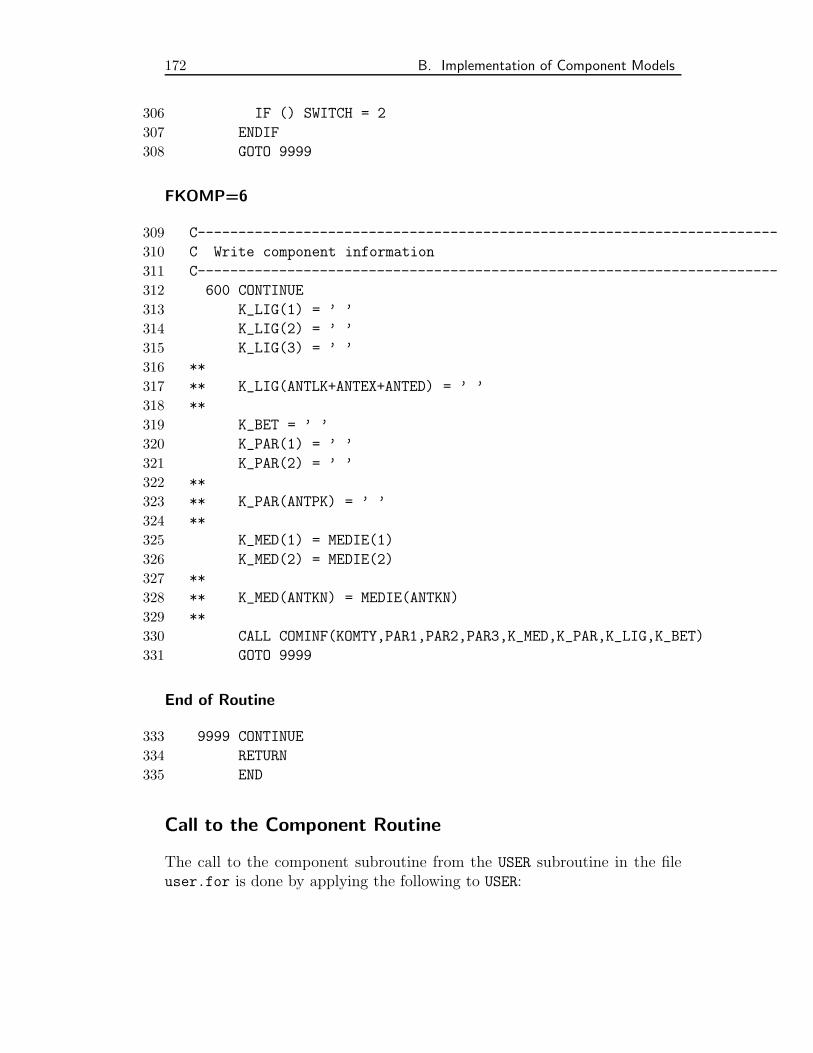
172 B. Implementation of Component Models
306 IF () SWITCH = 2
307 ENDIF
308 GOTO 9999
FKOMP=6
309 C-----------------------------------------------------------------------
310 C Write component information
311 C-----------------------------------------------------------------------
312 600 CONTINUE
313 K_LIG(1) = ’ ’
314 K_LIG(2) = ’ ’
315 K_LIG(3) = ’ ’
316 **
317 ** K_LIG(ANTLK+ANTEX+ANTED) = ’ ’
318 **
319 K_BET = ’ ’
320 K_PAR(1) = ’ ’
321 K_PAR(2) = ’ ’
322 **
323 ** K_PAR(ANTPK) = ’ ’
324 **
325 K_MED(1) = MEDIE(1)
326 K_MED(2) = MEDIE(2)
327 **
328 ** K_MED(ANTKN) = MEDIE(ANTKN)
329 **
330 CALL COMINF(KOMTY,PAR1,PAR2,PAR3,K_MED,K_PAR,K_LIG,K_BET)
331 GOTO 9999
End of Routine
333 9999 CONTINUE
334 RETURN
335 END
Call to the Component Routine
The call to the component subroutine from the USER subroutine in the fileuser.for is done by applying the following to USER:
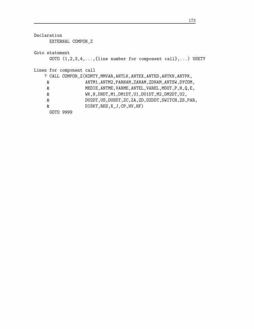
173
Declaration
EXTERNAL COMPON_Z
Goto statement
GOTO (1,2,3,4,...,line number for component call,...) USETY
Lines for component call
? CALL COMPON_Z(KOMTY,MMVAR,ANTLK,ANTEX,ANTED,ANTKN,ANTPK,
& ANTM1,ANTM2,PARNAM,ZANAM,ZDNAM,ANTSW,DYCOM,
& MEDIE,ANTME,VARME,ANTEL,VAREL,MDOT,P,H,Q,E,
& WK,N,DNDT,M1,DM1DT,U1,DU1DT,M2,DM2DT,U2,
& DU2DT,US,DUSDT,ZC,ZA,ZD,DZDDT,SWITCH,ZS,PAR,
& DISKT,RES,X_J,CP,HV,HF)
GOTO 9999

174 B. Implementation of Component Models
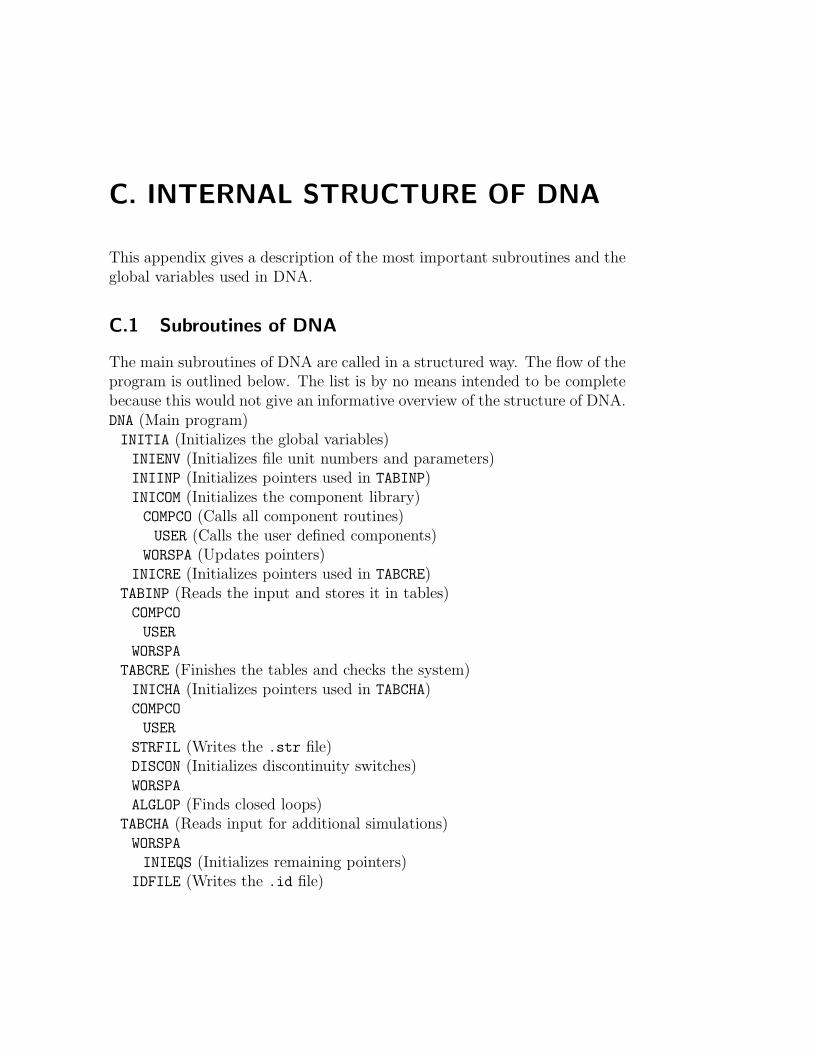
C. INTERNAL STRUCTURE OF DNA
This appendix gives a description of the most important subroutines and theglobal variables used in DNA.
C.1 Subroutines of DNA
The main subroutines of DNA are called in a structured way. The flow of theprogram is outlined below. The list is by no means intended to be completebecause this would not give an informative overview of the structure of DNA.DNA (Main program)INITIA (Initializes the global variables)INIENV (Initializes file unit numbers and parameters)INIINP (Initializes pointers used in TABINP)INICOM (Initializes the component library)COMPCO (Calls all component routines)USER (Calls the user defined components)
WORSPA (Updates pointers)INICRE (Initializes pointers used in TABCRE)
TABINP (Reads the input and stores it in tables)COMPCO
USER
WORSPA
TABCRE (Finishes the tables and checks the system)INICHA (Initializes pointers used in TABCHA)COMPCO
USER
STRFIL (Writes the .str file)DISCON (Initializes discontinuity switches)WORSPA
ALGLOP (Finds closed loops)TABCHA (Reads input for additional simulations)WORSPA
INIEQS (Initializes remaining pointers)IDFILE (Writes the .id file)
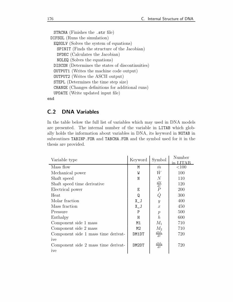
176 C. Internal Structure of DNA
STRCHA (Finishes the .str file)DIFSOL (Runs the simulation)EQSOLV (Solves the system of equations)SPINIT (Finds the structure of the Jacobian)DFDEC (Calculates the Jacobian)NOLEQ (Solves the equations)
DISCON (Determines the states of discontinuities)OUTPUT1 (Writes the machine code output)OUTPUT2 (Writes the ASCII output)STEPL (Determines the time step size)CHANGE (Changes definitions for additional runs)UPDATE (Write updated input file)
end
C.2 DNA Variables
In the table below the full list of variables which may used in DNA modelsare presented. The internal number of the variable in LITAB which glob-ally holds the information about variables in DNA, its keyword in NGTAB insubroutines TABINP.FOR and TABCHA.FOR and the symbol used for it in thethesis are provided.
Variable type Keyword SymbolNumberin LITAB
Mass flow M m <100
Mechanical power W W 100Shaft speed N N 110Shaft speed time derivative dN
dτ120
Electrical power E P 200
Heat Q Q 300Molar fraction X_J y 400Mass fraction X_J x 450Pressure P p 500Enthalpy H h 600Component side 1 mass M1 M1 710Component side 2 mass M2 M2 710Component side 1 mass time derivat-ive
DM1DT dM1
dτ720
Component side 2 mass time derivat-ive
DM2DT dM2
dτ720
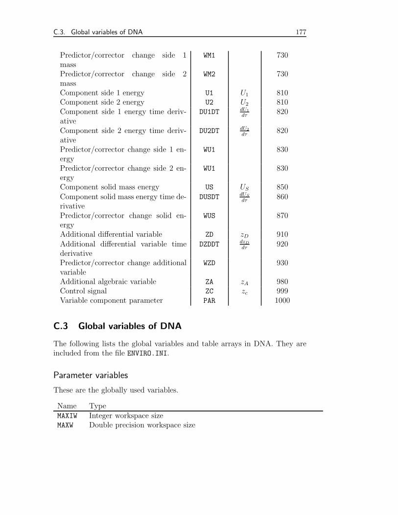
C.3. Global variables of DNA 177
Predictor/corrector change side 1mass
WM1 730
Predictor/corrector change side 2mass
WM2 730
Component side 1 energy U1 U1 810Component side 2 energy U2 U2 810Component side 1 energy time deriv-ative
DU1DT dU1
dτ820
Component side 2 energy time deriv-ative
DU2DT dU2
dτ820
Predictor/corrector change side 1 en-ergy
WU1 830
Predictor/corrector change side 2 en-ergy
WU1 830
Component solid mass energy US US 850
Component solid mass energy time de-rivative
DUSDT dUS
dτ860
Predictor/corrector change solid en-ergy
WUS 870
Additional differential variable ZD zD 910
Additional differential variable timederivative
DZDDT dzD
dτ920
Predictor/corrector change additionalvariable
WZD 930
Additional algebraic variable ZA zA 980Control signal ZC zc 999Variable component parameter PAR 1000
C.3 Global variables of DNA
The following lists the global variables and table arrays in DNA. They areincluded from the file ENVIRO.INI.
Parameter variables
These are the globally used variables.
Name TypeMAXIW Integer workspace sizeMAXW Double precision workspace size
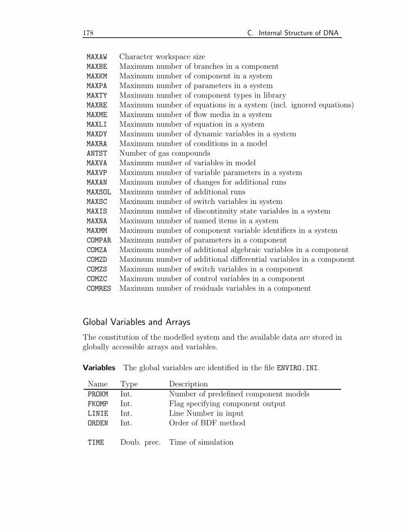
178 C. Internal Structure of DNA
MAXAW Character workspace sizeMAXBE Maximum number of branches in a componentMAXKM Maximum number of component in a systemMAXPA Maximum number of parameters in a systemMAXTY Maximum number of component types in libraryMAXRE Maximum number of equations in a system (incl. ignored equations)MAXME Maximum number of flow media in a systemMAXLI Maximum number of equation in a systemMAXDY Maximum number of dynamic variables in a systemMAXRA Maximum number of conditions in a modelANTST Number of gas compoundsMAXVA Maximum number of variables in modelMAXVP Maximum number of variable parameters in a systemMAXAN Maximum number of changes for additional runsMAXSOL Maximum number of additional runsMAXSC Maximum number of switch variables in systemMAXIS Maximum number of discontinuity state variables in a systemMAXNA Maximum number of named items in a systemMAXMM Maximum number of component variable identifiers in a systemCOMPAR Maximum number of parameters in a componentCOMZA Maximum number of additional algebraic variables in a componentCOMZD Maximum number of additional differential variables in a componentCOMZS Maximum number of switch variables in a componentCOMZC Maximum number of control variables in a componentCOMRES Maximum number of residuals variables in a component
Global Variables and Arrays
The constitution of the modelled system and the available data are stored inglobally accessible arrays and variables.
Variables The global variables are identified in the file ENVIRO.INI.
Name Type DescriptionPROKM Int. Number of predefined component modelsFKOMP Int. Flag specifying component outputLINIE Int. Line Number in inputORDEN Int. Order of BDF method
TIME Doub. prec. Time of simulation
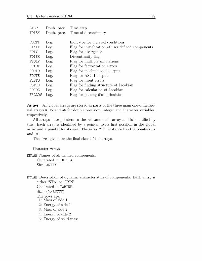
C.3. Global variables of DNA 179
STEP Doub. prec. Time stepTDISK Doub. prec. Time of discontinuity
FBETI Log. Indicator for violated conditionsFINIT Log. Flag for initialization of user defined componentsFDIV Log. Flag for divergenceFDISK Log. Discontinuity flagFSOLV Log. Flag for multiple simulationsFFACT Log. Flag for factorization errorsFOUTD Log. Flag for machine code outputFOUTS Log. Flag for ASCII outputFLSTO Log. Flag for input errorsFSTRU Log. Flag for finding structure of JacobianFDFDE Log. Flag for calculation of JacobianFALLOW Log. Flag for passing discontinuities
Arrays All global arrays are stored as parts of the three main one-dimensio-nal arrays W, IW and AW for double precision, integer and character variables,respectively.
All arrays have pointers to the relevant main array and is identified bythis. Each array is identified by a pointer to its first position in the globalarray and a pointer for its size. The array Y for instance has the pointers PYand DY.
The sizes given are the final sizes of the arrays.
Character Arrays
KMTAB Names of all defined components.Generated in INITIA
Size: ANTTY
DYTAB Description of dynamic characteristics of components. Each entry iseither ‘STA’ or ‘DYN’.Generated in TABINP.Size: (5×ANTTY)The rows are:1: Mass of side 12: Energy of side 13: Mass of side 24: Energy of side 25: Energy of solid mass
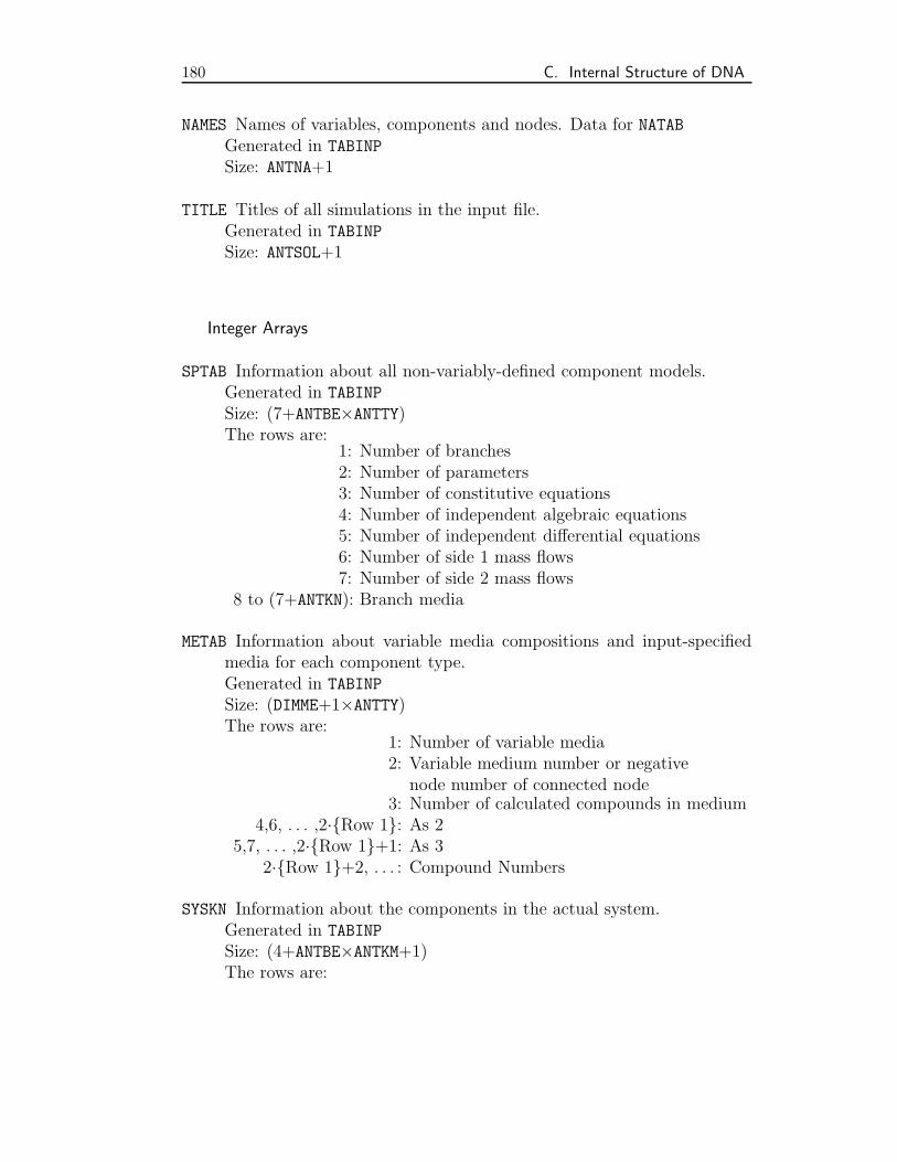
180 C. Internal Structure of DNA
NAMES Names of variables, components and nodes. Data for NATABGenerated in TABINP
Size: ANTNA+1
TITLE Titles of all simulations in the input file.Generated in TABINP
Size: ANTSOL+1
Integer Arrays
SPTAB Information about all non-variably-defined component models.Generated in TABINP
Size: (7+ANTBE×ANTTY)The rows are:
1: Number of branches2: Number of parameters3: Number of constitutive equations4: Number of independent algebraic equations5: Number of independent differential equations6: Number of side 1 mass flows7: Number of side 2 mass flows
8 to (7+ANTKN): Branch media
METAB Information about variable media compositions and input-specifiedmedia for each component type.Generated in TABINP
Size: (DIMME+1×ANTTY)The rows are:
1: Number of variable media2: Variable medium number or negative
node number of connected node3: Number of calculated compounds in medium
4,6, . . . ,2·Row 1: As 25,7, . . . ,2·Row 1+1: As 3
2·Row 1+2, . . . : Compound Numbers
SYSKN Information about the components in the actual system.Generated in TABINP
Size: (4+ANTBE×ANTKM+1)The rows are:
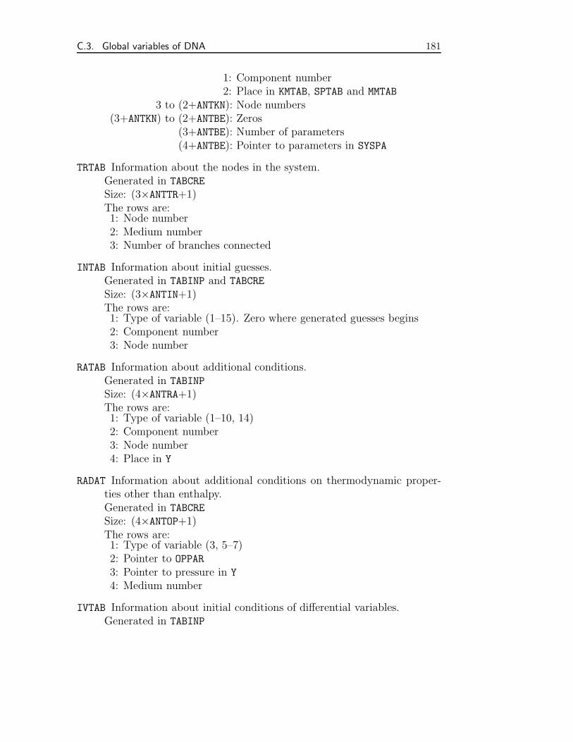
C.3. Global variables of DNA 181
1: Component number2: Place in KMTAB, SPTAB and MMTAB
3 to (2+ANTKN): Node numbers(3+ANTKN) to (2+ANTBE): Zeros
(3+ANTBE): Number of parameters(4+ANTBE): Pointer to parameters in SYSPA
TRTAB Information about the nodes in the system.Generated in TABCRE
Size: (3×ANTTR+1)The rows are:1: Node number2: Medium number3: Number of branches connected
INTAB Information about initial guesses.Generated in TABINP and TABCRE
Size: (3×ANTIN+1)The rows are:1: Type of variable (1–15). Zero where generated guesses begins2: Component number3: Node number
RATAB Information about additional conditions.Generated in TABINP
Size: (4×ANTRA+1)The rows are:1: Type of variable (1–10, 14)2: Component number3: Node number4: Place in Y
RADAT Information about additional conditions on thermodynamic proper-ties other than enthalpy.Generated in TABCRE
Size: (4×ANTOP+1)The rows are:1: Type of variable (3, 5–7)2: Pointer to OPPAR
3: Pointer to pressure in Y
4: Medium number
IVTAB Information about initial conditions of differential variables.Generated in TABINP
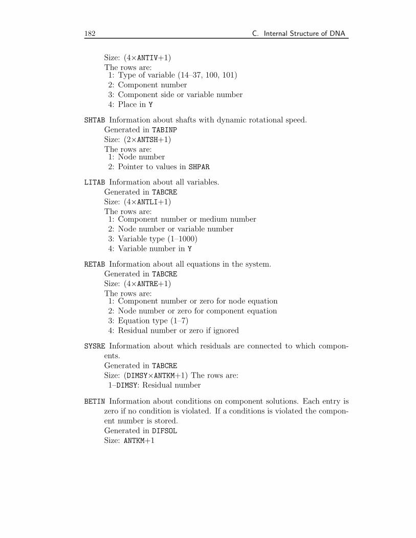
182 C. Internal Structure of DNA
Size: (4×ANTIV+1)The rows are:1: Type of variable (14–37, 100, 101)2: Component number3: Component side or variable number4: Place in Y
SHTAB Information about shafts with dynamic rotational speed.Generated in TABINP
Size: (2×ANTSH+1)The rows are:1: Node number2: Pointer to values in SHPAR
LITAB Information about all variables.Generated in TABCRE
Size: (4×ANTLI+1)The rows are:1: Component number or medium number2: Node number or variable number3: Variable type (1–1000)4: Variable number in Y
RETAB Information about all equations in the system.Generated in TABCRE
Size: (4×ANTRE+1)The rows are:1: Component number or zero for node equation2: Node number or zero for component equation3: Equation type (1–7)4: Residual number or zero if ignored
SYSRE Information about which residuals are connected to which compon-ents.Generated in TABCRE
Size: (DIMSY×ANTKM+1) The rows are:1–DIMSY: Residual number
BETIN Information about conditions on component solutions. Each entry iszero if no condition is violated. If a conditions is violated the compon-ent number is stored.Generated in DIFSOL
Size: ANTKM+1
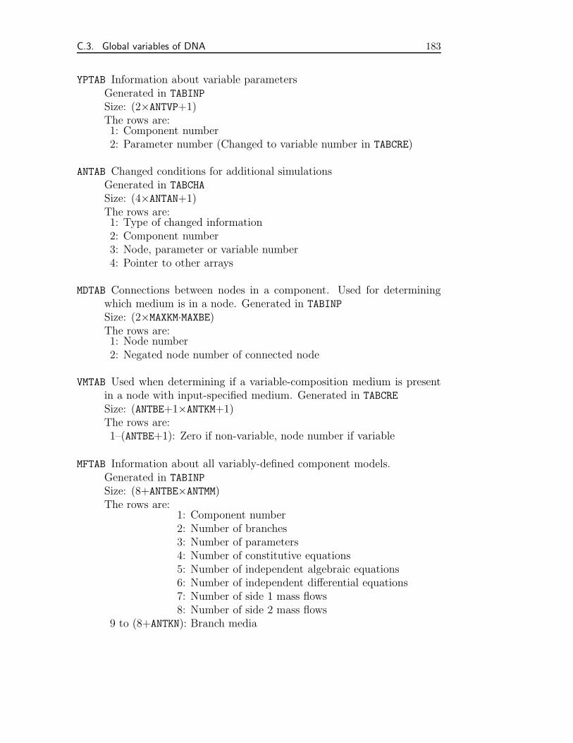
C.3. Global variables of DNA 183
YPTAB Information about variable parametersGenerated in TABINP
Size: (2×ANTVP+1)The rows are:1: Component number2: Parameter number (Changed to variable number in TABCRE)
ANTAB Changed conditions for additional simulationsGenerated in TABCHA
Size: (4×ANTAN+1)The rows are:1: Type of changed information2: Component number3: Node, parameter or variable number4: Pointer to other arrays
MDTAB Connections between nodes in a component. Used for determiningwhich medium is in a node. Generated in TABINP
Size: (2×MAXKM·MAXBE)The rows are:1: Node number2: Negated node number of connected node
VMTAB Used when determining if a variable-composition medium is presentin a node with input-specified medium. Generated in TABCRE
Size: (ANTBE+1×ANTKM+1)The rows are:1–(ANTBE+1): Zero if non-variable, node number if variable
MFTAB Information about all variably-defined component models.Generated in TABINP
Size: (8+ANTBE×ANTMM)The rows are:
1: Component number2: Number of branches3: Number of parameters4: Number of constitutive equations5: Number of independent algebraic equations6: Number of independent differential equations7: Number of side 1 mass flows8: Number of side 2 mass flows
9 to (8+ANTKN): Branch media
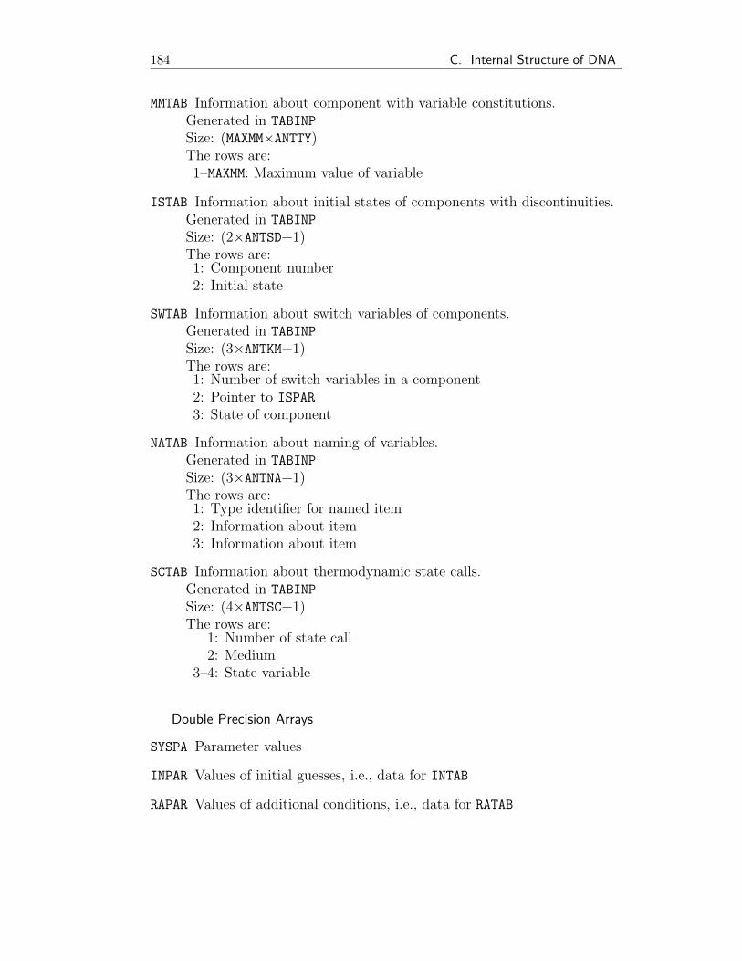
184 C. Internal Structure of DNA
MMTAB Information about component with variable constitutions.Generated in TABINP
Size: (MAXMM×ANTTY)The rows are:1–MAXMM: Maximum value of variable
ISTAB Information about initial states of components with discontinuities.Generated in TABINP
Size: (2×ANTSD+1)The rows are:1: Component number2: Initial state
SWTAB Information about switch variables of components.Generated in TABINP
Size: (3×ANTKM+1)The rows are:1: Number of switch variables in a component2: Pointer to ISPAR
3: State of component
NATAB Information about naming of variables.Generated in TABINP
Size: (3×ANTNA+1)The rows are:1: Type identifier for named item2: Information about item3: Information about item
SCTAB Information about thermodynamic state calls.Generated in TABINP
Size: (4×ANTSC+1)The rows are:
1: Number of state call2: Medium
3–4: State variable
Double Precision Arrays
SYSPA Parameter values
INPAR Values of initial guesses, i.e., data for INTAB
RAPAR Values of additional conditions, i.e., data for RATAB
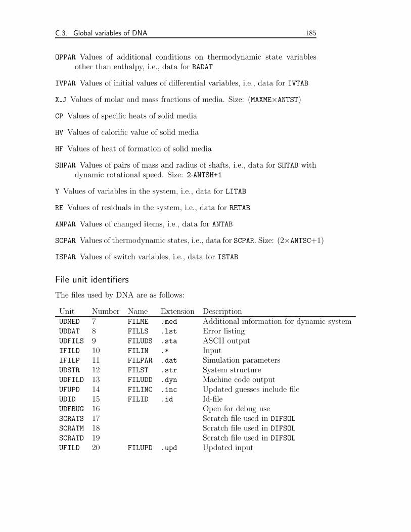
C.3. Global variables of DNA 185
OPPAR Values of additional conditions on thermodynamic state variablesother than enthalpy, i.e., data for RADAT
IVPAR Values of initial values of differential variables, i.e., data for IVTAB
X J Values of molar and mass fractions of media. Size: (MAXME×ANTST)
CP Values of specific heats of solid media
HV Values of calorific value of solid media
HF Values of heat of formation of solid media
SHPAR Values of pairs of mass and radius of shafts, i.e., data for SHTAB withdynamic rotational speed. Size: 2·ANTSH+1
Y Values of variables in the system, i.e., data for LITAB
RE Values of residuals in the system, i.e., data for RETAB
ANPAR Values of changed items, i.e., data for ANTAB
SCPAR Values of thermodynamic states, i.e., data for SCPAR. Size: (2×ANTSC+1)
ISPAR Values of switch variables, i.e., data for ISTAB
File unit identifiers
The files used by DNA are as follows:
Unit Number Name Extension DescriptionUDMED 7 FILME .med Additional information for dynamic systemUDDAT 8 FILLS .lst Error listingUDFILS 9 FILUDS .sta ASCII outputIFILD 10 FILIN .* InputIFILP 11 FILPAR .dat Simulation parametersUDSTR 12 FILST .str System structureUDFILD 13 FILUDD .dyn Machine code outputUFUPD 14 FILINC .inc Updated guesses include fileUDID 15 FILID .id Id-fileUDEBUG 16 Open for debug useSCRATS 17 Scratch file used in DIFSOL
SCRATM 18 Scratch file used in DIFSOL
SCRATD 19 Scratch file used in DIFSOL
UFILD 20 FILUPD .upd Updated input
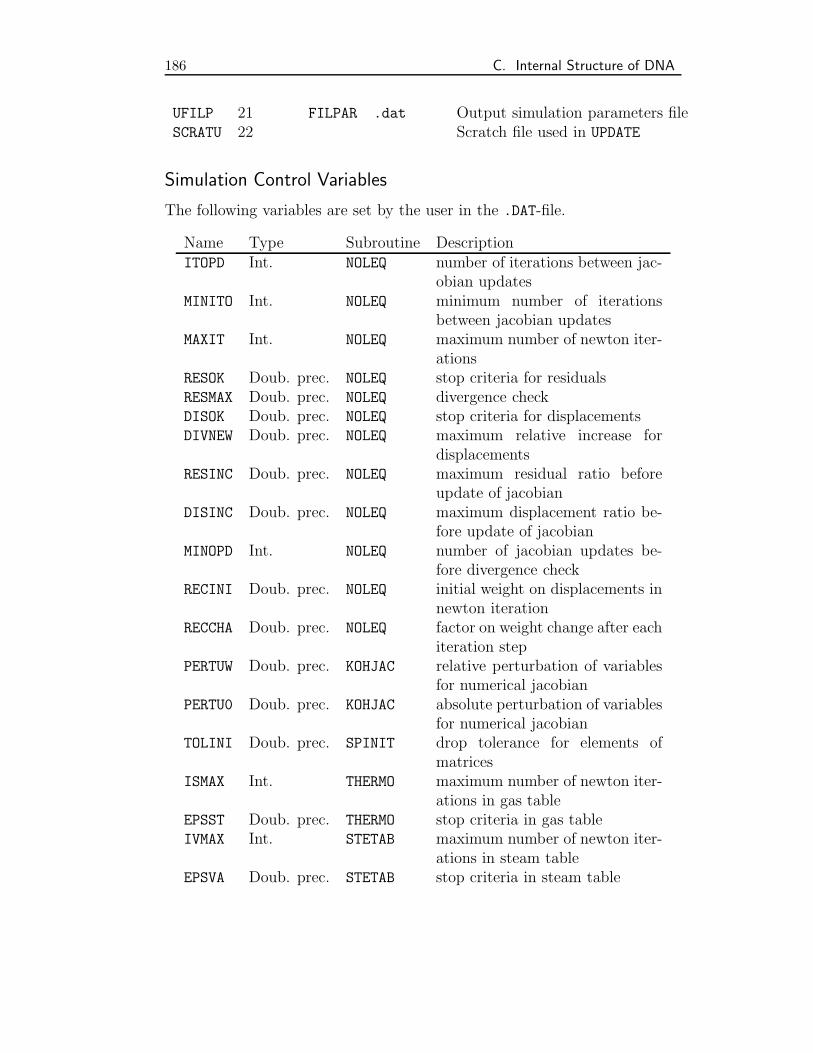
186 C. Internal Structure of DNA
UFILP 21 FILPAR .dat Output simulation parameters fileSCRATU 22 Scratch file used in UPDATE
Simulation Control Variables
The following variables are set by the user in the .DAT-file.
Name Type Subroutine DescriptionITOPD Int. NOLEQ number of iterations between jac-
obian updatesMINITO Int. NOLEQ minimum number of iterations
between jacobian updatesMAXIT Int. NOLEQ maximum number of newton iter-
ationsRESOK Doub. prec. NOLEQ stop criteria for residualsRESMAX Doub. prec. NOLEQ divergence checkDISOK Doub. prec. NOLEQ stop criteria for displacementsDIVNEW Doub. prec. NOLEQ maximum relative increase for
displacementsRESINC Doub. prec. NOLEQ maximum residual ratio before
update of jacobianDISINC Doub. prec. NOLEQ maximum displacement ratio be-
fore update of jacobianMINOPD Int. NOLEQ number of jacobian updates be-
fore divergence checkRECINI Doub. prec. NOLEQ initial weight on displacements in
newton iterationRECCHA Doub. prec. NOLEQ factor on weight change after each
iteration stepPERTUW Doub. prec. KOHJAC relative perturbation of variables
for numerical jacobianPERTU0 Doub. prec. KOHJAC absolute perturbation of variables
for numerical jacobianTOLINI Doub. prec. SPINIT drop tolerance for elements of
matricesISMAX Int. THERMO maximum number of newton iter-
ations in gas tableEPSST Doub. prec. THERMO stop criteria in gas tableIVMAX Int. STETAB maximum number of newton iter-
ations in steam tableEPSVA Doub. prec. STETAB stop criteria in steam table
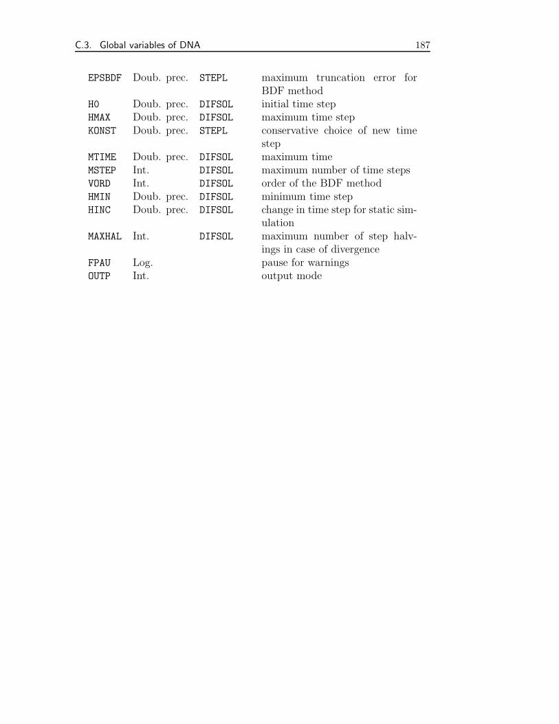
C.3. Global variables of DNA 187
EPSBDF Doub. prec. STEPL maximum truncation error forBDF method
H0 Doub. prec. DIFSOL initial time stepHMAX Doub. prec. DIFSOL maximum time stepKONST Doub. prec. STEPL conservative choice of new time
stepMTIME Doub. prec. DIFSOL maximum timeMSTEP Int. DIFSOL maximum number of time stepsVORD Int. DIFSOL order of the BDF methodHMIN Doub. prec. DIFSOL minimum time stepHINC Doub. prec. DIFSOL change in time step for static sim-
ulationMAXHAL Int. DIFSOL maximum number of step halv-
ings in case of divergenceFPAU Log. pause for warningsOUTP Int. output mode

188 C. Internal Structure of DNA
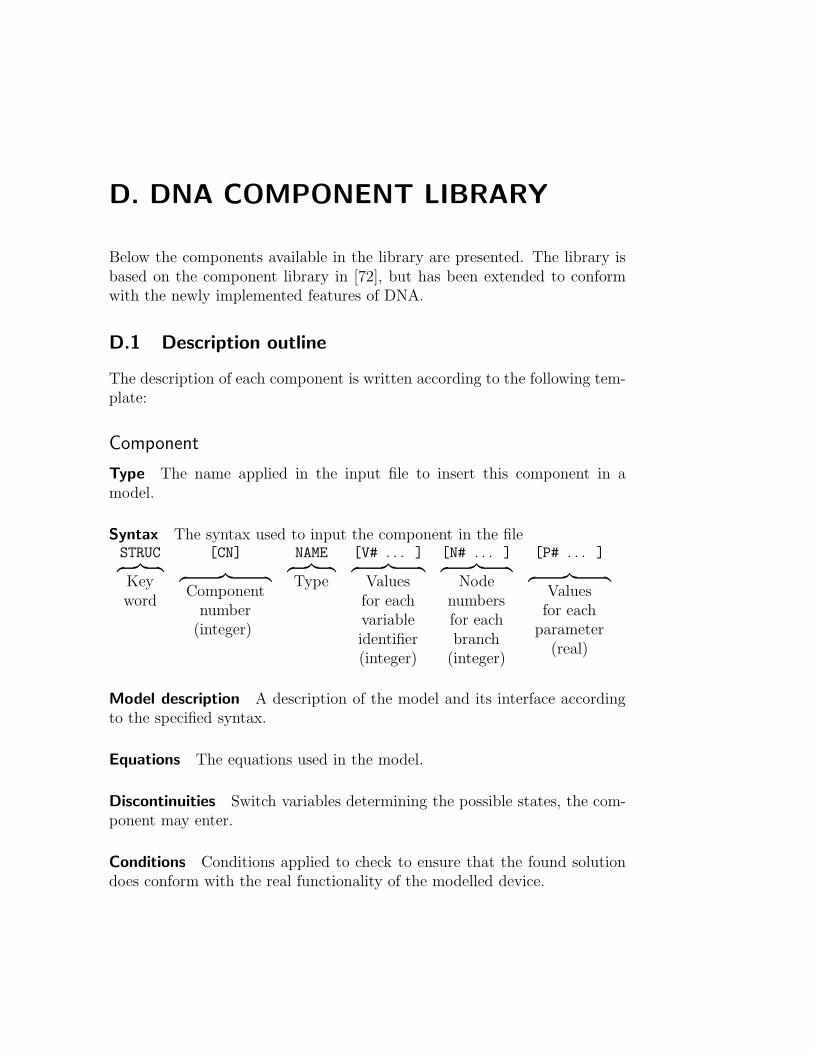
D. DNA COMPONENT LIBRARY
Below the components available in the library are presented. The library isbased on the component library in [72], but has been extended to conformwith the newly implemented features of DNA.
D.1 Description outline
The description of each component is written according to the following tem-plate:
Component
Type The name applied in the input file to insert this component in amodel.
Syntax The syntax used to input the component in the fileSTRUC [CN] NAME [V# . . . ] [N# . . . ] [P# . . . ]︷ ︸︸ ︷Keyword
︷ ︸︸ ︷Componentnumber(integer)
︷ ︸︸ ︷Type
︷ ︸︸ ︷Valuesfor eachvariableidentifier(integer)
︷ ︸︸ ︷Node
numbersfor eachbranch(integer)
︷ ︸︸ ︷Valuesfor eachparameter(real)
Model description A description of the model and its interface accordingto the specified syntax.
Equations The equations used in the model.
Discontinuities Switch variables determining the possible states, the com-ponent may enter.
Conditions Conditions applied to check to ensure that the found solutiondoes conform with the real functionality of the modelled device.
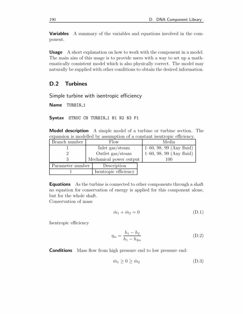
190 D. DNA Component Library
Variables A summary of the variables and equations involved in the com-ponent.
Usage A short explanation on how to work with the component in a model.The main aim of this usage is to provide users with a way to set up a math-ematically consistent model which is also physically correct. The model maynaturally be supplied with other conditions to obtain the desired information.
D.2 Turbines
Simple turbine with isentropic efficiency
Name TURBIN 1
Syntax STRUC CN TURBIN 1 N1 N2 N3 P1
Model description A simple model of a turbine or turbine section. Theexpansion is modelled by assumption of a constant isentropic efficiency.Branch number Flow Media
1 Inlet gas/steam 1–60, 98, 99 (Any fluid)2 Outlet gas/steam 1–60, 98, 99 (Any fluid)3 Mechanical power output 100
Parameter number Description1 Isentropic efficiency
Equations As the turbine is connected to other components through a shaftno equation for conservation of energy is applied for this component alone,but for the whole shaft.Conservation of mass
m1 + m2 = 0 (D.1)
Isentropic efficiency
ηis =h1 − h2
h1 − h2is
(D.2)
Conditions Mass flow from high pressure end to low pressure end:
m1 ≥ 0 ≥ m2 (D.3)
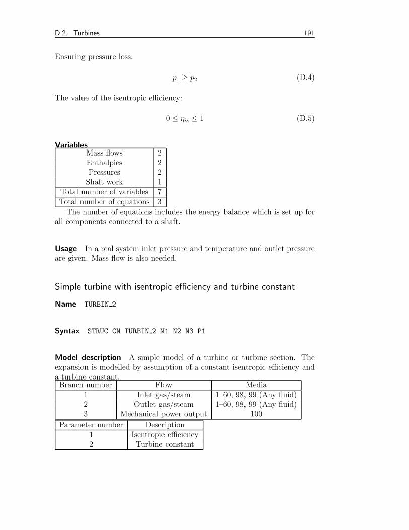
D.2. Turbines 191
Ensuring pressure loss:
p1 ≥ p2 (D.4)
The value of the isentropic efficiency:
0 ≤ ηis ≤ 1 (D.5)
VariablesMass flows 2Enthalpies 2Pressures 2Shaft work 1
Total number of variables 7Total number of equations 3
The number of equations includes the energy balance which is set up forall components connected to a shaft.
Usage In a real system inlet pressure and temperature and outlet pressureare given. Mass flow is also needed.
Simple turbine with isentropic efficiency and turbine constant
Name TURBIN 2
Syntax STRUC CN TURBIN 2 N1 N2 N3 P1
Model description A simple model of a turbine or turbine section. Theexpansion is modelled by assumption of a constant isentropic efficiency anda turbine constant.Branch number Flow Media
1 Inlet gas/steam 1–60, 98, 99 (Any fluid)2 Outlet gas/steam 1–60, 98, 99 (Any fluid)3 Mechanical power output 100
Parameter number Description1 Isentropic efficiency2 Turbine constant
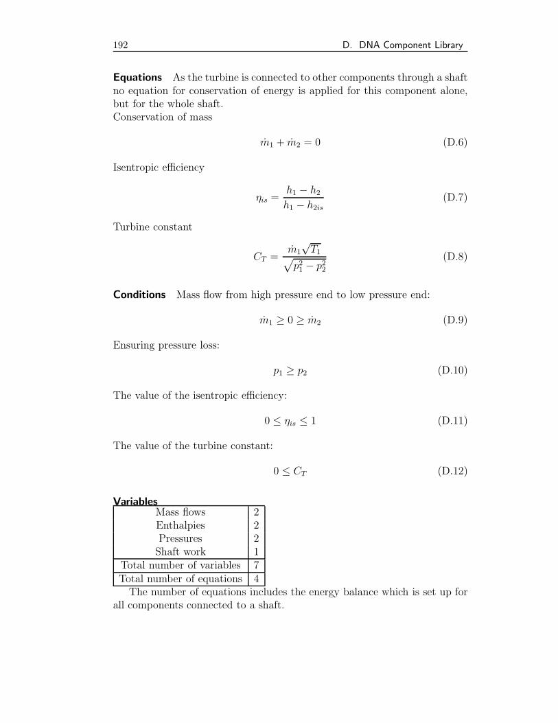
192 D. DNA Component Library
Equations As the turbine is connected to other components through a shaftno equation for conservation of energy is applied for this component alone,but for the whole shaft.Conservation of mass
m1 + m2 = 0 (D.6)
Isentropic efficiency
ηis =h1 − h2
h1 − h2is
(D.7)
Turbine constant
CT =m1
√T1√
p21 − p2
2
(D.8)
Conditions Mass flow from high pressure end to low pressure end:
m1 ≥ 0 ≥ m2 (D.9)
Ensuring pressure loss:
p1 ≥ p2 (D.10)
The value of the isentropic efficiency:
0 ≤ ηis ≤ 1 (D.11)
The value of the turbine constant:
0 ≤ CT (D.12)
VariablesMass flows 2Enthalpies 2Pressures 2Shaft work 1
Total number of variables 7Total number of equations 4The number of equations includes the energy balance which is set up for
all components connected to a shaft.
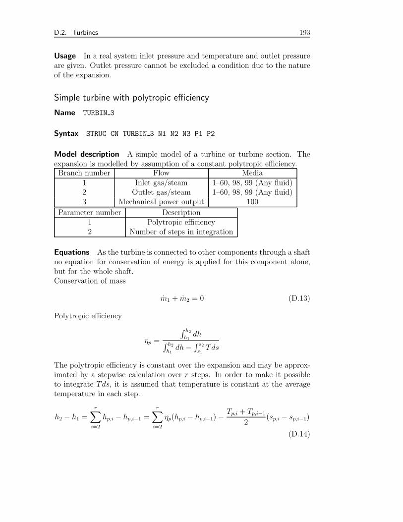
D.2. Turbines 193
Usage In a real system inlet pressure and temperature and outlet pressureare given. Outlet pressure cannot be excluded a condition due to the natureof the expansion.
Simple turbine with polytropic efficiency
Name TURBIN 3
Syntax STRUC CN TURBIN 3 N1 N2 N3 P1 P2
Model description A simple model of a turbine or turbine section. Theexpansion is modelled by assumption of a constant polytropic efficiency.Branch number Flow Media
1 Inlet gas/steam 1–60, 98, 99 (Any fluid)2 Outlet gas/steam 1–60, 98, 99 (Any fluid)3 Mechanical power output 100
Parameter number Description1 Polytropic efficiency2 Number of steps in integration
Equations As the turbine is connected to other components through a shaftno equation for conservation of energy is applied for this component alone,but for the whole shaft.Conservation of mass
m1 + m2 = 0 (D.13)
Polytropic efficiency
ηp =
∫ h2
h1dh∫ h2
h1dh− ∫ s2
s1Tds
The polytropic efficiency is constant over the expansion and may be approx-imated by a stepwise calculation over r steps. In order to make it possibleto integrate Tds, it is assumed that temperature is constant at the averagetemperature in each step.
h2 − h1 =
r∑i=2
hp,i − hp,i−1 =
r∑i=2
ηp(hp,i − hp,i−1)− Tp,i + Tp,i−1
2(sp,i − sp,i−1)
(D.14)
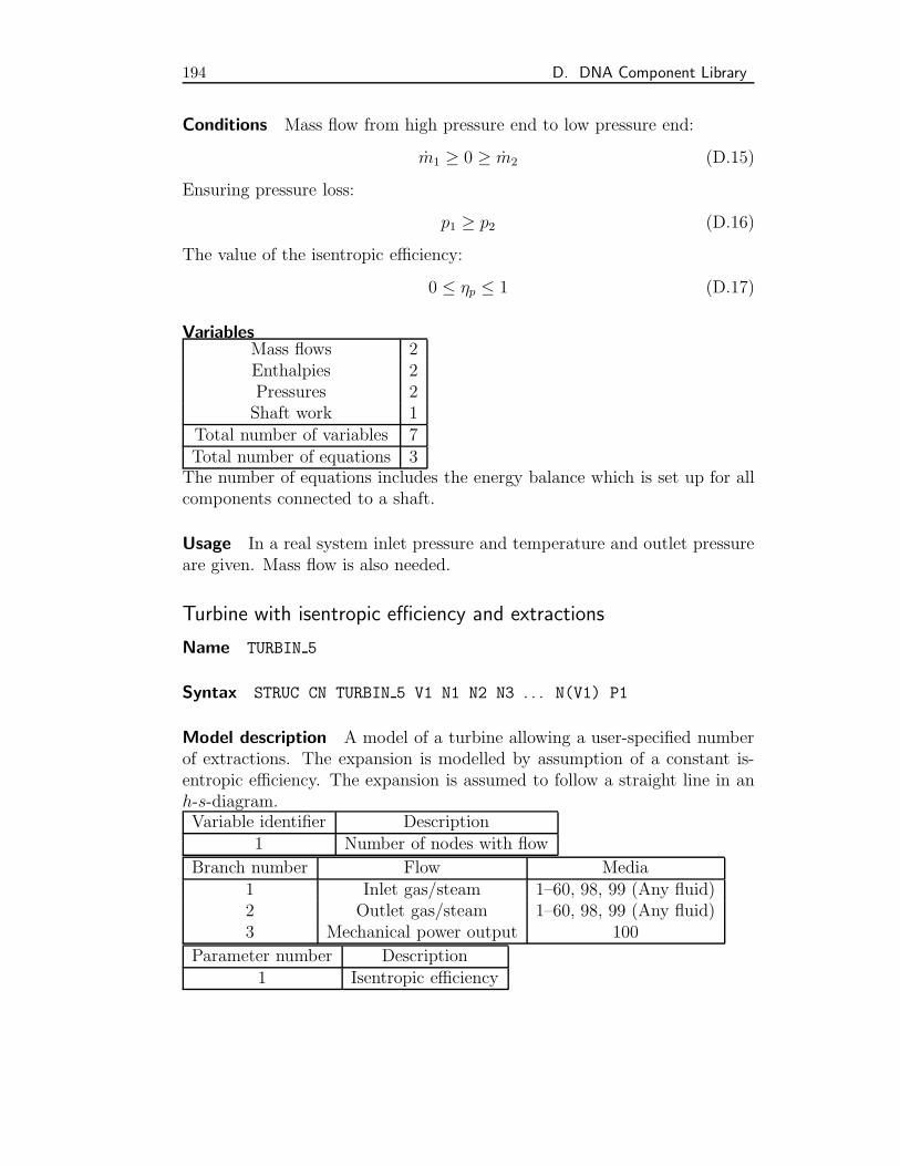
194 D. DNA Component Library
Conditions Mass flow from high pressure end to low pressure end:
m1 ≥ 0 ≥ m2 (D.15)
Ensuring pressure loss:
p1 ≥ p2 (D.16)
The value of the isentropic efficiency:
0 ≤ ηp ≤ 1 (D.17)
VariablesMass flows 2Enthalpies 2Pressures 2Shaft work 1
Total number of variables 7Total number of equations 3The number of equations includes the energy balance which is set up for allcomponents connected to a shaft.
Usage In a real system inlet pressure and temperature and outlet pressureare given. Mass flow is also needed.
Turbine with isentropic efficiency and extractions
Name TURBIN 5
Syntax STRUC CN TURBIN 5 V1 N1 N2 N3 . . . N(V1) P1
Model description A model of a turbine allowing a user-specified numberof extractions. The expansion is modelled by assumption of a constant is-entropic efficiency. The expansion is assumed to follow a straight line in anh-s-diagram.Variable identifier Description
1 Number of nodes with flow
Branch number Flow Media1 Inlet gas/steam 1–60, 98, 99 (Any fluid)2 Outlet gas/steam 1–60, 98, 99 (Any fluid)3 Mechanical power output 100
Parameter number Description1 Isentropic efficiency
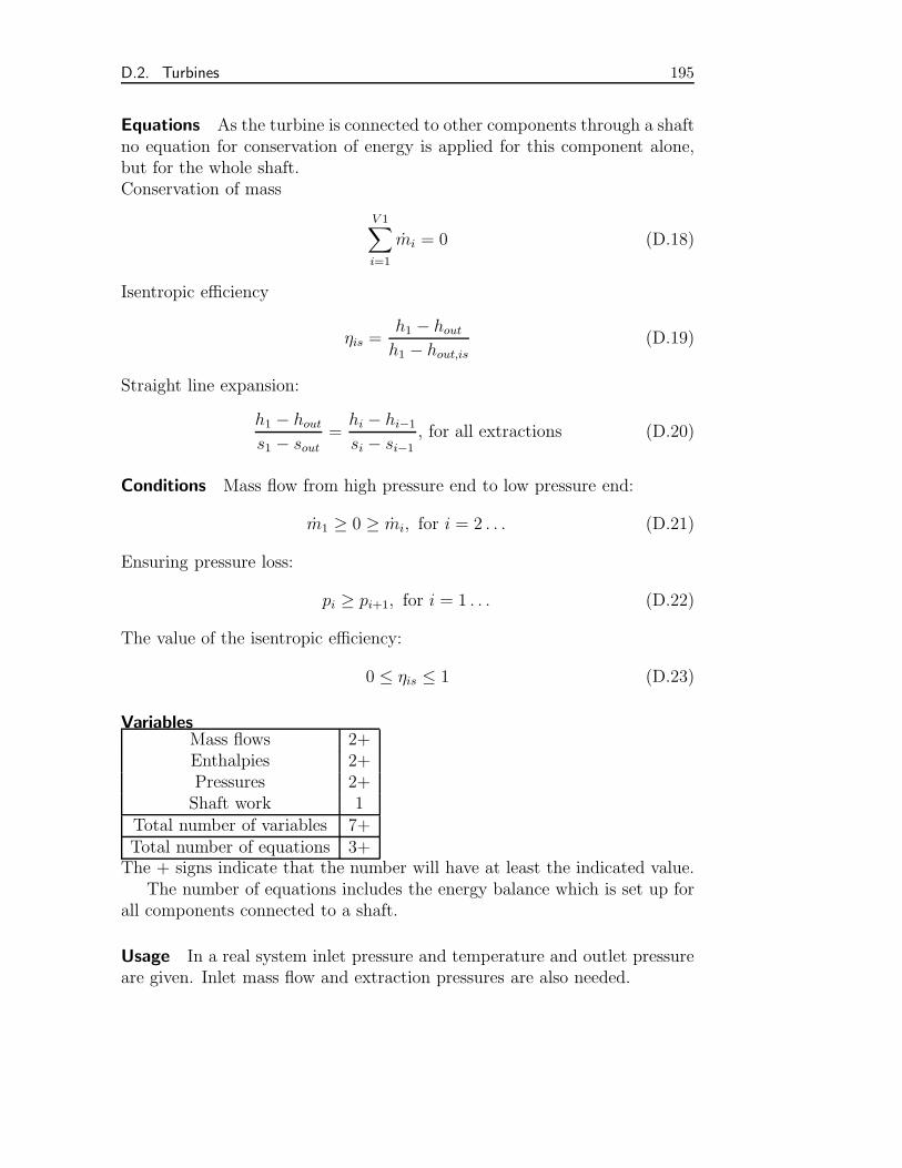
D.2. Turbines 195
Equations As the turbine is connected to other components through a shaftno equation for conservation of energy is applied for this component alone,but for the whole shaft.Conservation of mass
V 1∑i=1
mi = 0 (D.18)
Isentropic efficiency
ηis =h1 − houth1 − hout,is
(D.19)
Straight line expansion:
h1 − houts1 − sout
=hi − hi−1
si − si−1
, for all extractions (D.20)
Conditions Mass flow from high pressure end to low pressure end:
m1 ≥ 0 ≥ mi, for i = 2 . . . (D.21)
Ensuring pressure loss:
pi ≥ pi+1, for i = 1 . . . (D.22)
The value of the isentropic efficiency:
0 ≤ ηis ≤ 1 (D.23)
VariablesMass flows 2+Enthalpies 2+Pressures 2+Shaft work 1
Total number of variables 7+Total number of equations 3+The + signs indicate that the number will have at least the indicated value.
The number of equations includes the energy balance which is set up forall components connected to a shaft.
Usage In a real system inlet pressure and temperature and outlet pressureare given. Inlet mass flow and extraction pressures are also needed.
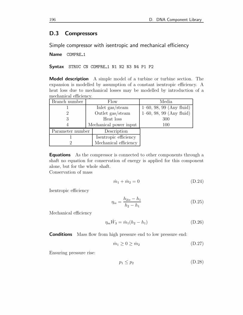
196 D. DNA Component Library
D.3 Compressors
Simple compressor with isentropic and mechanical efficiency
Name COMPRE 1
Syntax STRUC CN COMPRE 1 N1 N2 N3 N4 P1 P2
Model description A simple model of a turbine or turbine section. Theexpansion is modelled by assumption of a constant isentropic efficiency. Aheat loss due to mechanical losses may be modelled by introduction of amechanical efficiency.Branch number Flow Media
1 Inlet gas/steam 1–60, 98, 99 (Any fluid)2 Outlet gas/steam 1–60, 98, 99 (Any fluid)3 Heat loss 3004 Mechanical power input 100
Parameter number Description1 Isentropic efficiency2 Mechanical efficiency
Equations As the compressor is connected to other components through ashaft no equation for conservation of energy is applied for this componentalone, but for the whole shaft.Conservation of mass
m1 + m2 = 0 (D.24)
Isentropic efficiency
ηis =h2is − h1
h2 − h1
(D.25)
Mechanical efficiency
ηmW3 = m1(h2 − h1) (D.26)
Conditions Mass flow from high pressure end to low pressure end:
m1 ≥ 0 ≥ m2 (D.27)
Ensuring pressure rise:
p1 ≤ p2 (D.28)
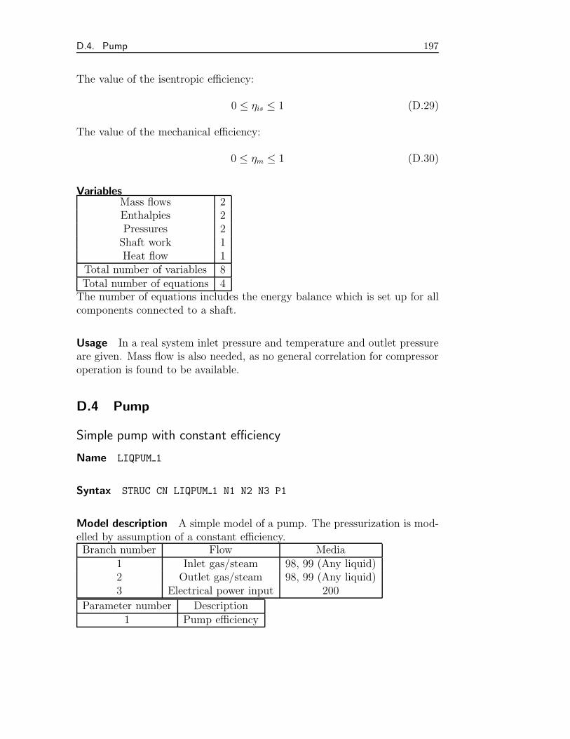
D.4. Pump 197
The value of the isentropic efficiency:
0 ≤ ηis ≤ 1 (D.29)
The value of the mechanical efficiency:
0 ≤ ηm ≤ 1 (D.30)
VariablesMass flows 2Enthalpies 2Pressures 2Shaft work 1Heat flow 1
Total number of variables 8Total number of equations 4The number of equations includes the energy balance which is set up for allcomponents connected to a shaft.
Usage In a real system inlet pressure and temperature and outlet pressureare given. Mass flow is also needed, as no general correlation for compressoroperation is found to be available.
D.4 Pump
Simple pump with constant efficiency
Name LIQPUM 1
Syntax STRUC CN LIQPUM 1 N1 N2 N3 P1
Model description A simple model of a pump. The pressurization is mod-elled by assumption of a constant efficiency.Branch number Flow Media
1 Inlet gas/steam 98, 99 (Any liquid)2 Outlet gas/steam 98, 99 (Any liquid)3 Electrical power input 200
Parameter number Description1 Pump efficiency
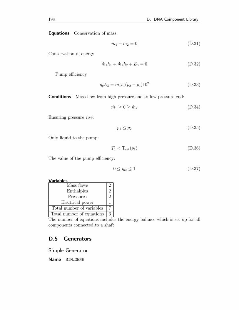
198 D. DNA Component Library
Equations Conservation of mass
m1 + m2 = 0 (D.31)
Conservation of energy
m1h1 + m2h2 + E3 = 0 (D.32)
Pump efficiency
ηpE3 = m1v1(p2 − p1)102 (D.33)
Conditions Mass flow from high pressure end to low pressure end:
m1 ≥ 0 ≥ m2 (D.34)
Ensuring pressure rise:
p1 ≤ p2 (D.35)
Only liquid to the pump:
T1 < Tsat(p1) (D.36)
The value of the pump efficiency:
0 ≤ ηis ≤ 1 (D.37)
VariablesMass flows 2Enthalpies 2Pressures 2
Electrical power 1Total number of variables 7Total number of equations 3The number of equations includes the energy balance which is set up for allcomponents connected to a shaft.
D.5 Generators
Simple Generator
Name SIM GENE
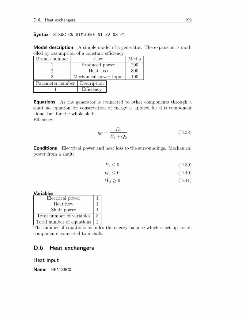
D.6. Heat exchangers 199
Syntax STRUC CN SIM GENE N1 N2 N3 P1
Model description A simple model of a generator. The expansion is mod-elled by assumption of a constant efficiency.Branch number Flow Media
1 Produced power 2002 Heat loss 3003 Mechanical power input 100
Parameter number Description1 Efficiency
Equations As the generator is connected to other components through ashaft no equation for conservation of energy is applied for this componentalone, but for the whole shaft.Efficiency
ηG =E1
E1 + Q2
(D.38)
Conditions Electrical power and heat loss to the surroundings. Mechanicalpower from a shaft:
E1 ≤ 0 (D.39)
Q2 ≤ 0 (D.40)
W3 ≥ 0 (D.41)
VariablesElectrical power 1
Heat flow 1Shaft power 1
Total number of variables 3Total number of equations 2The number of equations includes the energy balance which is set up for allcomponents connected to a shaft.
D.6 Heat exchangers
Heat input
Name HEATSRC0
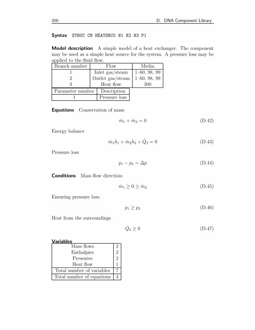
200 D. DNA Component Library
Syntax STRUC CN HEATSRC0 N1 N2 N3 P1
Model description A simple model of a heat exchanger. The componentmay be used as a simple heat source for the system. A pressure loss may beapplied to the fluid flow.Branch number Flow Media
1 Inlet gas/steam 1–60, 98, 992 Outlet gas/steam 1–60, 98, 993 Heat flow 300
Parameter number Description1 Pressure loss
Equations Conservation of mass
m1 + m2 = 0 (D.42)
Energy balance
m1h1 + m2h2 + Q3 = 0 (D.43)
Pressure loss
p1 − p2 = ∆p (D.44)
Conditions Mass flow direction:
m1 ≥ 0 ≥ m2 (D.45)
Ensuring pressure loss:
p1 ≥ p2 (D.46)
Heat from the surroundings
Q3 ≥ 0 (D.47)
VariablesMass flows 2Enthalpies 2Pressures 2Heat flow 1
Total number of variables 7Total number of equations 4
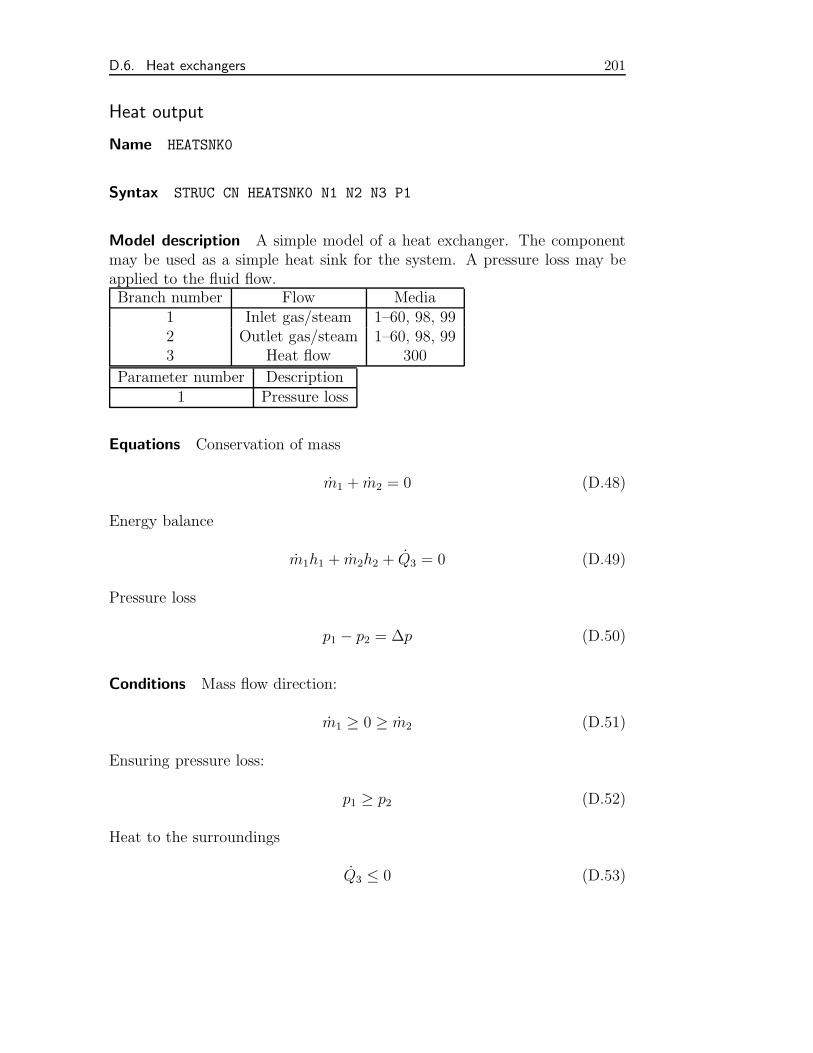
D.6. Heat exchangers 201
Heat output
Name HEATSNK0
Syntax STRUC CN HEATSNK0 N1 N2 N3 P1
Model description A simple model of a heat exchanger. The componentmay be used as a simple heat sink for the system. A pressure loss may beapplied to the fluid flow.Branch number Flow Media
1 Inlet gas/steam 1–60, 98, 992 Outlet gas/steam 1–60, 98, 993 Heat flow 300
Parameter number Description1 Pressure loss
Equations Conservation of mass
m1 + m2 = 0 (D.48)
Energy balance
m1h1 + m2h2 + Q3 = 0 (D.49)
Pressure loss
p1 − p2 = ∆p (D.50)
Conditions Mass flow direction:
m1 ≥ 0 ≥ m2 (D.51)
Ensuring pressure loss:
p1 ≥ p2 (D.52)
Heat to the surroundings
Q3 ≤ 0 (D.53)
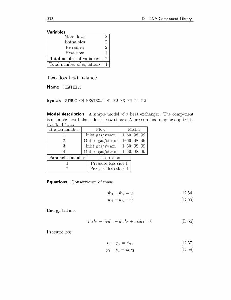
202 D. DNA Component Library
VariablesMass flows 2Enthalpies 2Pressures 2Heat flow 1
Total number of variables 7Total number of equations 4
Two flow heat balance
Name HEATEX 1
Syntax STRUC CN HEATEX 1 N1 N2 N3 N4 P1 P2
Model description A simple model of a heat exchanger. The componentis a simple heat balance for the two flows. A pressure loss may be applied tothe fluid flows.Branch number Flow Media
1 Inlet gas/steam 1–60, 98, 992 Outlet gas/steam 1–60, 98, 993 Inlet gas/steam 1–60, 98, 994 Outlet gas/steam 1–60, 98, 99
Parameter number Description1 Pressure loss side I2 Pressure loss side II
Equations Conservation of mass
m1 + m2 = 0 (D.54)
m3 + m4 = 0 (D.55)
Energy balance
m1h1 + m2h2 + m3h3 + m4h4 = 0 (D.56)
Pressure loss
p1 − p2 = ∆pI (D.57)
p3 − p4 = ∆pII (D.58)
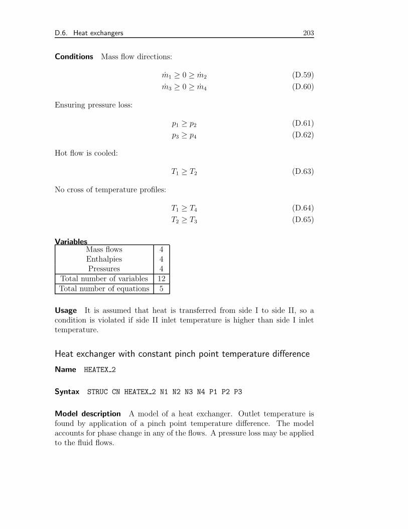
D.6. Heat exchangers 203
Conditions Mass flow directions:
m1 ≥ 0 ≥ m2 (D.59)
m3 ≥ 0 ≥ m4 (D.60)
Ensuring pressure loss:
p1 ≥ p2 (D.61)
p3 ≥ p4 (D.62)
Hot flow is cooled:
T1 ≥ T2 (D.63)
No cross of temperature profiles:
T1 ≥ T4 (D.64)
T2 ≥ T3 (D.65)
VariablesMass flows 4Enthalpies 4Pressures 4
Total number of variables 12Total number of equations 5
Usage It is assumed that heat is transferred from side I to side II, so acondition is violated if side II inlet temperature is higher than side I inlettemperature.
Heat exchanger with constant pinch point temperature difference
Name HEATEX 2
Syntax STRUC CN HEATEX 2 N1 N2 N3 N4 P1 P2 P3
Model description A model of a heat exchanger. Outlet temperature isfound by application of a pinch point temperature difference. The modelaccounts for phase change in any of the flows. A pressure loss may be appliedto the fluid flows.
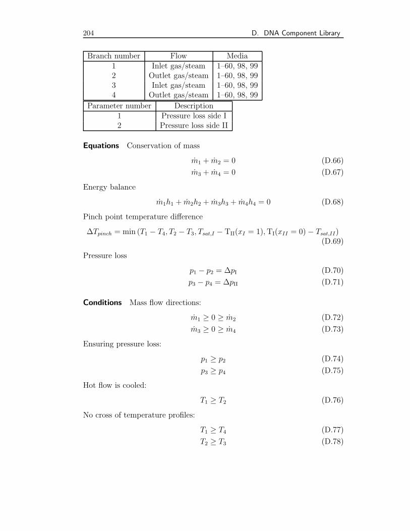
204 D. DNA Component Library
Branch number Flow Media1 Inlet gas/steam 1–60, 98, 992 Outlet gas/steam 1–60, 98, 993 Inlet gas/steam 1–60, 98, 994 Outlet gas/steam 1–60, 98, 99
Parameter number Description1 Pressure loss side I2 Pressure loss side II
Equations Conservation of mass
m1 + m2 = 0 (D.66)
m3 + m4 = 0 (D.67)
Energy balance
m1h1 + m2h2 + m3h3 + m4h4 = 0 (D.68)
Pinch point temperature difference
∆Tpinch = min (T1 − T4, T2 − T3, Tsat,I − TII(xI = 1),TI(xII = 0)− Tsat,II)(D.69)
Pressure loss
p1 − p2 = ∆pI (D.70)
p3 − p4 = ∆pII (D.71)
Conditions Mass flow directions:
m1 ≥ 0 ≥ m2 (D.72)
m3 ≥ 0 ≥ m4 (D.73)
Ensuring pressure loss:
p1 ≥ p2 (D.74)
p3 ≥ p4 (D.75)
Hot flow is cooled:
T1 ≥ T2 (D.76)
No cross of temperature profiles:
T1 ≥ T4 (D.77)
T2 ≥ T3 (D.78)
D.6. Heat exchangers 205
VariablesMass flows 4Enthalpies 4Pressures 4
Total number of variables 12Total number of equations 6
Usage It is assumed that heat is transferred from side I to side II, so acondition is violated if side II inlet temperature is higher than side I inlettemperature.
Two flow heat exchanger with heat transfer coefficient
Name HEATEX 3
Syntax STRUC CN HEATEX 3 N1 N2 N3 N4 P1 P2 P3 P4
Model description A simple model of a heat exchanger. The heat exchangeis governed by a heat transfer coefficient and a surface area. A pressure lossmay be applied to the fluid flows.Branch number Flow Media
1 Inlet gas/steam 1–60, 98, 992 Outlet gas/steam 1–60, 98, 993 Inlet gas/steam 1–60, 98, 994 Outlet gas/steam 1–60, 98, 99
Parameter number Description1 Heat transfer coefficient2 Surface Area3 Pressure loss side I4 Pressure loss side II
Equations Conservation of mass
m1 + m2 = 0 (D.79)
m3 + m4 = 0 (D.80)
Energy balance
m1h1 + m2h2 + m3h3 + m4h4 = 0 (D.81)
206 D. DNA Component Library
Heat transfer relation
m1h1 + m2h2 =
UA(T1 − T4)− (T2 − T3)
lnT1 − T4
T2 − T3
, for mIcp,I = mIIcp,II
UA(T1 − T4), for mIcp,I = mIIcp,II
(D.82)
Pressure loss
p1 − p2 = ∆pI (D.83)
p3 − p4 = ∆pII (D.84)
Conditions Mass flow directions:
m1 ≥ 0 ≥ m2 (D.85)
m3 ≥ 0 ≥ m4 (D.86)
Ensuring pressure loss:
p1 ≥ p2 (D.87)
p3 ≥ p4 (D.88)
Hot flow is cooled:
T1 ≥ T2 (D.89)
No cross of temperature profiles:
T1 ≥ T4 (D.90)
T2 ≥ T3 (D.91)
VariablesMass flows 4Enthalpies 4Pressures 4
Total number of variables 12Total number of equations 6
Usage It is assumed that heat is transferred from side I to side II, so acondition is violated if side II inlet temperature is higher than side I inlettemperature. The heat transfer equation (D.82) is undefined if the temperat-ure values supplied make the temperature profiles cross. The model handlesthis situation by applying a zero temperature difference at the end, wherethe temperatures should be closest.
D.6. Heat exchangers 207
Two flow heat exchanger with effectiveness
Name HEATEX 4
Syntax STRUC CN HEATEX 4 N1 N2 N3 N4 P1 P2 P3
Model description A simple model of a heat exchanger. The heat exchangeis governed by an effectiveness. A pressure loss may be applied to the fluidflows.Branch number Flow Media
1 Inlet gas/steam 1–60, 98, 992 Outlet gas/steam 1–60, 98, 993 Inlet gas/steam 1–60, 98, 994 Outlet gas/steam 1–60, 98, 99
Parameter number Description1 Heat transfer effectiveness2 Pressure loss side I3 Pressure loss side II
Equations Conservation of mass
m1 + m2 = 0 (D.92)
m3 + m4 = 0 (D.93)
Energy balance
m1h1 + m2h2 + m3h3 + m4h4 = 0 (D.94)
Heat transfer effectiveness
ε =
T4 − T3
T1 − T3
, for mIcp,I ≥ mIIcp,II
T1 − T2
T1 − T3
, for mIcp,I < mIIcp,II
(D.95)
Pressure loss
p1 − p2 = ∆pI (D.96)
p3 − p4 = ∆pII (D.97)
208 D. DNA Component Library
Conditions Mass flow directions:
m1 ≥ 0 ≥ m2 (D.98)
m3 ≥ 0 ≥ m4 (D.99)
Ensuring pressure loss:
p1 ≥ p2 (D.100)
p3 ≥ p4 (D.101)
Hot flow is cooled:
T1 ≥ T2 (D.102)
No cross of temperature profiles:
T1 ≥ T4 (D.103)
T2 ≥ T3 (D.104)
VariablesMass flows 4Enthalpies 4Pressures 4
Total number of variables 12Total number of equations 6
Usage It is assumed that heat is transferred from side I to side II, so acondition is violated if side II inlet temperature is higher than side I inlettemperature.
Two flow heat exchanger with heat transfer coefficient andgoverning dynamic effects
Name HEATEX 7
Syntax STRUC CN HEATEX 7 N1 N2 N3 N4 P1 P2 P3 P4 P5 P6
Model description A model of a heat exchanger. The heat exchange isgoverned by a heat transfer coefficient and a surface area. A pressure lossmay be applied to the fluid flows. Mass and internal energy of both fluidsides are considered to be dynamic.
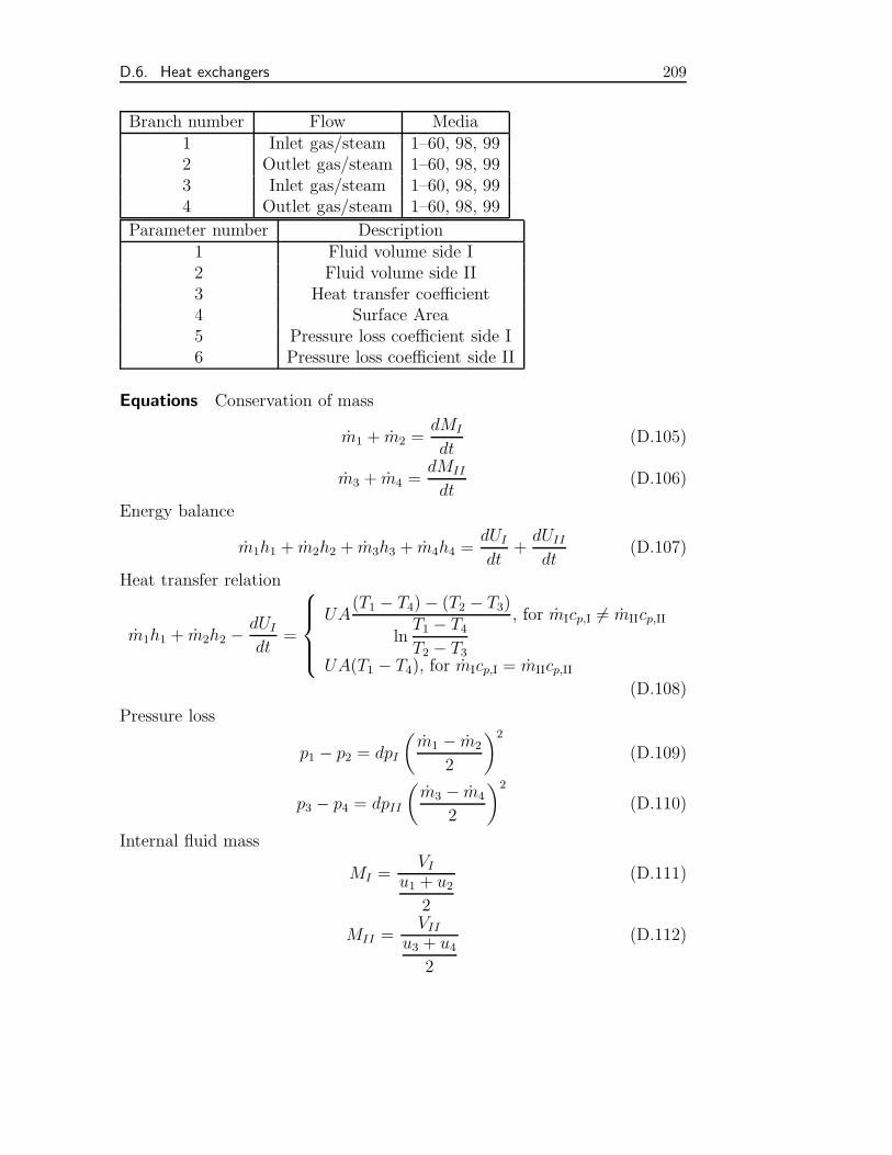
D.6. Heat exchangers 209
Branch number Flow Media1 Inlet gas/steam 1–60, 98, 992 Outlet gas/steam 1–60, 98, 993 Inlet gas/steam 1–60, 98, 994 Outlet gas/steam 1–60, 98, 99
Parameter number Description1 Fluid volume side I2 Fluid volume side II3 Heat transfer coefficient4 Surface Area5 Pressure loss coefficient side I6 Pressure loss coefficient side II
Equations Conservation of mass
m1 + m2 =dMI
dt(D.105)
m3 + m4 =dMII
dt(D.106)
Energy balance
m1h1 + m2h2 + m3h3 + m4h4 =dUI
dt+dUII
dt(D.107)
Heat transfer relation
m1h1 + m2h2 − dUI
dt=
UA(T1 − T4)− (T2 − T3)
lnT1 − T4
T2 − T3
, for mIcp,I = mIIcp,II
UA(T1 − T4), for mIcp,I = mIIcp,II(D.108)
Pressure loss
p1 − p2 = dpI
(m1 − m2
2
)2
(D.109)
p3 − p4 = dpII
(m3 − m4
2
)2
(D.110)
Internal fluid mass
MI =VI
u1 + u2
2
(D.111)
MII =VII
u3 + u4
2
(D.112)
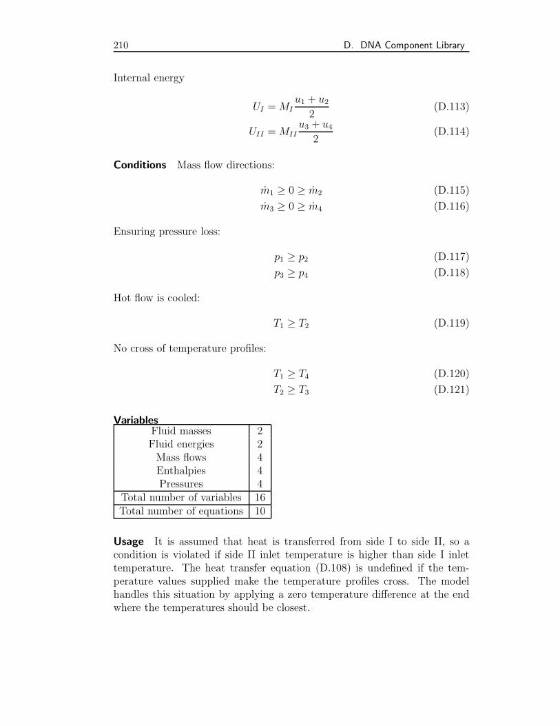
210 D. DNA Component Library
Internal energy
UI =MIu1 + u2
2(D.113)
UII =MIIu3 + u4
2(D.114)
Conditions Mass flow directions:
m1 ≥ 0 ≥ m2 (D.115)
m3 ≥ 0 ≥ m4 (D.116)
Ensuring pressure loss:
p1 ≥ p2 (D.117)
p3 ≥ p4 (D.118)
Hot flow is cooled:
T1 ≥ T2 (D.119)
No cross of temperature profiles:
T1 ≥ T4 (D.120)
T2 ≥ T3 (D.121)
VariablesFluid masses 2Fluid energies 2Mass flows 4Enthalpies 4Pressures 4
Total number of variables 16Total number of equations 10
Usage It is assumed that heat is transferred from side I to side II, so acondition is violated if side II inlet temperature is higher than side I inlettemperature. The heat transfer equation (D.108) is undefined if the tem-perature values supplied make the temperature profiles cross. The modelhandles this situation by applying a zero temperature difference at the endwhere the temperatures should be closest.
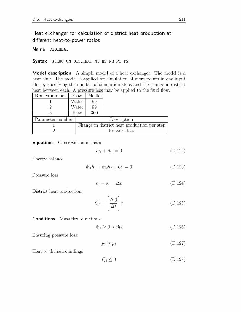
D.6. Heat exchangers 211
Heat exchanger for calculation of district heat production atdifferent heat-to-power ratios
Name DIS HEAT
Syntax STRUC CN DIS HEAT N1 N2 N3 P1 P2
Model description A simple model of a heat exchanger. The model is aheat sink. The model is applied for simulation of more points in one inputfile, by specifying the number of simulation steps and the change in districtheat between each. A pressure loss may be applied to the fluid flow.Branch number Flow Media
1 Water 992 Water 993 Heat 300
Parameter number Description1 Change in district heat production per step2 Pressure loss
Equations Conservation of mass
m1 + m2 = 0 (D.122)
Energy balance
m1h1 + m2h2 + Q3 = 0 (D.123)
Pressure loss
p1 − p2 = ∆p (D.124)
District heat production
Q3 =
[∆Q
∆t
]t (D.125)
Conditions Mass flow directions:
m1 ≥ 0 ≥ m2 (D.126)
Ensuring pressure loss:
p1 ≥ p2 (D.127)
Heat to the surroundings
Q3 ≤ 0 (D.128)
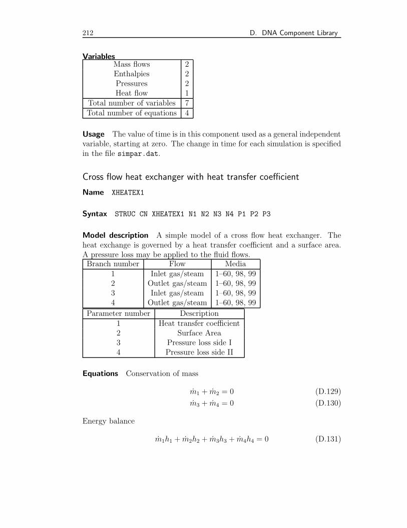
212 D. DNA Component Library
VariablesMass flows 2Enthalpies 2Pressures 2Heat flow 1
Total number of variables 7Total number of equations 4
Usage The value of time is in this component used as a general independentvariable, starting at zero. The change in time for each simulation is specifiedin the file simpar.dat.
Cross flow heat exchanger with heat transfer coefficient
Name XHEATEX1
Syntax STRUC CN XHEATEX1 N1 N2 N3 N4 P1 P2 P3
Model description A simple model of a cross flow heat exchanger. Theheat exchange is governed by a heat transfer coefficient and a surface area.A pressure loss may be applied to the fluid flows.Branch number Flow Media
1 Inlet gas/steam 1–60, 98, 992 Outlet gas/steam 1–60, 98, 993 Inlet gas/steam 1–60, 98, 994 Outlet gas/steam 1–60, 98, 99
Parameter number Description1 Heat transfer coefficient2 Surface Area3 Pressure loss side I4 Pressure loss side II
Equations Conservation of mass
m1 + m2 = 0 (D.129)
m3 + m4 = 0 (D.130)
Energy balance
m1h1 + m2h2 + m3h3 + m4h4 = 0 (D.131)
D.6. Heat exchangers 213
Heat transfer relation
m1h1 + m2h2 =
FTUA(T1 − T4)− (T2 − T3)
lnT1 − T4
T2 − T3
, for mIcp,I = mIIcp,II
FTUA(T1 − T4), for mIcp,I = mIIcp,II(D.132)
Pressure loss
p1 − p2 = ∆pI (D.133)
p3 − p4 = ∆pII (D.134)
Conditions Mass flow directions:
m1 ≥ 0 ≥ m2 (D.135)
m3 ≥ 0 ≥ m4 (D.136)
Ensuring pressure loss:
p1 ≥ p2 (D.137)
p3 ≥ p4 (D.138)
Hot flow is cooled:
T1 ≥ T2 (D.139)
No cross of temperature profiles:
T1 ≥ T4 (D.140)
T2 ≥ T3 (D.141)
VariablesMass flows 4Enthalpies 4Pressures 4
Total number of variables 12Total number of equations 6
Usage It is assumed that heat is transferred from side I to side II, so acondition is violated if side II inlet temperature is higher than side I inlettemperature. The heat transfer equation (D.132) is undefined if the tem-perature values supplied make the temperature profiles cross. The modelhandles this situation by applying a zero temperature difference at the end,where the temperatures are closest.
214 D. DNA Component Library
D.7 Boilers and Evaporators
Simple boiler model
Name SIM BOIL
Syntax STRUC CN SIM BOIL N1 N2 N3 P1
Model description A simple model of a boiler. The component is a simpleheat source for the system. A pressure loss may be applied to the fluid flow.Branch number Flow Media
1 CO2 or water 98, 992 CO2 or water 98, 993 Heat flow 300
Parameter number Description1 Pressure loss
Equations Conservation of mass
m1 + m2 = 0 (D.142)
Energy balance
m1h1 + m2h2 + Q3 = 0 (D.143)
Pressure loss
p1 − p2 = ∆p (D.144)
Conditions Mass flow direction:
m1 ≥ 0 ≥ m2 (D.145)
Ensuring pressure loss:
p1 ≥ p2 (D.146)
Heat from the surroundings
Q3 ≥ 0 (D.147)
Ensuring evaporation
T2 ≥ Tsat(p2) (D.148)
D.8. Condensers 215
VariablesMass flows 2Enthalpies 2Pressures 2Heat flow 1
Total number of variables 7Total number of equations 3
D.8 Condensers
Condenser to Heat output
Name CONDEN 0
Syntax STRUC CN CONDEN 0 N1 N2 N3 P1
Model description A simple model of a condenser. The component maybe used as a simple heat sink for the system. A pressure loss may be appliedto the fluid flow.Branch number Flow Media
1 Inlet vapour 98, 992 Outlet liquid 98, 993 Heat flow 300
Parameter number Description1 Pressure loss
Equations Conservation of mass
m1 + m2 = 0 (D.149)
Energy balance
m1h1 + m2h2 + Q3 = 0 (D.150)
Saturated liquid
x2 = 0 (D.151)
Pressure loss
p1 − p2 = ∆p (D.152)
216 D. DNA Component Library
Conditions Mass flow direction:
m1 ≥ 0 ≥ m2 (D.153)
Ensuring pressure loss:
p1 ≥ p2 (D.154)
Heat to the surroundings
Q3 ≤ 0 (D.155)
VariablesMass flows 2Enthalpies 2Pressures 2Heat flow 1
Total number of variables 7Total number of equations 5
Simple condenser
Name CONDEN 1
Syntax STRUC CN CONDEN 1 N1 N2 N3 N4 P1 P2
Model description A simple model of a condenser. The component is asimple heat balance for the two flows. A pressure loss may be applied to thefluid flows.Branch number Flow Media
1 Inlet vapour 98, 992 Outlet liquid 98, 993 Inlet fluid 1–60, 98, 994 Outlet fluid 1–60, 98, 99
Parameter number Description1 Pressure loss side I2 Pressure loss side II
Equations Conservation of mass
m1 + m2 = 0 (D.156)
m3 + m4 = 0 (D.157)
D.8. Condensers 217
Energy balance
m1h1 + m2h2 + m3h3 + m4h4 = 0 (D.158)
Saturated liquid
x2 = 0 (D.159)
Pressure loss
p1 − p2 = ∆pI (D.160)
p3 − p4 = ∆pII (D.161)
Conditions Mass flow directions:
m1 ≥ 0 ≥ m2 (D.162)
m3 ≥ 0 ≥ m4 (D.163)
Ensuring pressure loss:
p1 ≥ p2 (D.164)
p3 ≥ p4 (D.165)
Hot flow is cooled:
T1 ≥ T2 (D.166)
No cross of temperature profiles:
T1 ≥ T4 (D.167)
T2 ≥ T3 (D.168)
VariablesMass flows 4Enthalpies 4Pressures 4
Total number of variables 13Total number of equations 5
Usage It is assumed that heat is transferred from side I to side II, so acondition is violated if side II inlet temperature is higher than side I inlettemperature.
218 D. DNA Component Library
Feedwater tank
Name DEAERA 1
Syntax STRUC CN DEAERA 1 V1 N1 N2 N3 . . . P1 P2
Model description A simple model of a deaerator. A pressure loss may beapplied to the fluid.Branch number Flow Media
1 Inlet vapour 98, 992 Inlet vapour 98, 993 Inlet liquid 98, 99
. . .n Outlet fluid 98, 99
Parameter number Description1 Pressure loss
Equations Conservation of mass∑mi = 0 (D.169)
Energy balance ∑mihi = 0 (D.170)
Saturated liquid
xn = 0 (D.171)
Pressure loss
p1 − pn = ∆p (D.172)
Conditions Mass flow directions:
mi ≥ 0, for i = 1, n− 1 (D.173)
0 ≥ mn (D.174)
Ensuring pressure loss:
D.9. Dryers 219
VariablesMass flows 3+Enthalpies 3+Pressures 3+
Total number of variables 9+Total number of equations 3The +’s indicate that the figures are minimum values.
D.9 Dryers
Name DRYER 01
Syntax STRUC CN DRYER 01 N1 N2 N3 N4 N5 P1 P2
Model description A direct-contact solid fuel dryer, where hot gas is usedfor evaporation of moisture from a solid fuel.Branch number Flow Media
1 Inlet fuel 1-40, 61-80 (Any solid)2 Inlet gas 1–60 (Any gas)3 Outlet fuel 1-40, 61-80 (Any solid)4 Outlet gas 1–60 (Any gas)5 Heat loss 300
Parameter number Description1 Fuel outlet moisture content2 Gas pressure loss
Equations Conservation of mass
m1 + m2 + m3 + m4 = 0 (D.175)
Conservation of energy
m1h1 + m2h2 + m3h3 + m4h4 + Q5 = 0 (D.176)
Temperature of outlet flows are equal
T2 = T3 (D.177)
Outlet Pressures
p2 − p4 = ∆p (D.178)
220 D. DNA Component Library
Mass flow relation between moist and dry fuel
m1(1− x1,H2O) + m3(1− x3,H2O) (D.179)
Fuel outlet composition
x3 = x(x1) (D.180)
Gas outlet composition
y4= y(x1, y2
, m1, m2) (D.181)
Conditions Mass flow directions
m1 ≥ 0 (D.182)
m2 ≥ 0 (D.183)
m3 ≤ 0 (D.184)
m4 ≤ 0 (D.185)
Heat flow to surroundings
Q5 ≤ 0 (D.186)
Moisture content of fuel is decreased
x1,H2O ≥ x3,H2O (D.187)
VariablesMass flows 4Enthalpies 4Pressures 4Heat flow 1
Molar fractions 38Mass fractions 38
Total number of variables 89Total number of equations 77
D.10 Burners
Combustor for ideal gas with constant air-to-fuel ratio
Name GASBUR 1
D.10. Burners 221
Syntax STRUC CN GASBUR 1 N1 N2 N3 N4 P1 P2
Model description A simple model of a combustion chamber for gasses,i.e., for a gas turbine. The model only allows gasses with a constant com-position to be used. Outlet pressure is given as a fraction of the inlet pressure.Branch number Flow Media
1 Inlet air 1–60 (Any constant composition gas)2 Outlet gaseous fuel 1–60 (Any constant composition gas)3 Outlet flue gas 1–60 (Any constant composition gas)4 Heat loss 300
Parameter number Description1 Air-to-fuel ratio2 Outlet–inlet pressure ratio
Equations Conservation of mass
m1 + m2 + m3 = 0 (D.188)
Energy balance
m1h1 + m2h2 + m3h3 + Q4 = 0 (D.189)
Pressures
p2 = p1 (D.190)p3
p1= PR (D.191)
Air-to-fuel ratio
AF =m1
m2(D.192)
Conditions Mass flow directions:
m1 ≥ 0 (D.193)
m2 ≥ 0 (D.194)
0 ≥ m3 (D.195)
Ensuring pressure loss:
p1 ≥ p2 (D.196)
222 D. DNA Component Library
Stoichiometric combustion
AF ≥ AFmin (D.197)
Heat to surroundings
Q4 ≤ 0 (D.198)
VariablesMass flows 3Enthalpies 3Pressures 3Heat flow 1
Total number of variables 10Total number of equations 5
Usage This model should be used carefully and may be considered obsolete,because it does not check if the supplied gasses in fact do not change compos-ition during simulation. If gasses which change their composition are used,the model will still find a solution but it will be based on the compositionsupplied by initial guesses. The same happens if AF is made variable.
Combustor for ideal gas with given outlet temperature
Name GASBUR 2
Syntax STRUC CN GASBUR 2 N1 N2 N3 N4 P1 P2
Model description A model of a combustion chamber for gasses, i.e., for agas turbine. Outlet pressure is given as a fraction of the inlet pressure.Branch number Flow Media
1 Inlet air 1–60 (Any gas)2 Outlet gaseous fuel 1–60 (Any gas)3 Outlet flue gas 1–60 (Any gas)4 Heat loss 300
Parameter number Description1 Outlet temperature2 Outlet–inlet pressure ratio
D.10. Burners 223
Equations Conservation of mass
m1 + m2 + m3 = 0 (D.199)
Energy balance
m1h1 + m2h2 + m3h3 + Q4 = 0 (D.200)
Pressures
p2 = p1 (D.201)p3
p1
= PR (D.202)
Flue gas temperature
h3 = h(Tout) (D.203)
Flue gas composition:
y3= y(m1, m2, h1, h2, h3, y1
, y2)
calculated for O2, N2, CO2, H2O, SO2 and Ar (D.204)
Conditions Mass flow directions:
m1 ≥ 0 (D.205)
m2 ≥ 0 (D.206)
0 ≥ m3 (D.207)
Ensuring pressure loss:
p1 ≥ p2 (D.208)
Stoichiometric combustion
AF ≥ AFmin (D.209)
Heat to surroundings
Q4 ≤ 0 (D.210)
224 D. DNA Component Library
VariablesMass flows 3Enthalpies 3Pressures 3Heat flow 1
Molar fractions 6+Total number of variables 16+Total number of equations 11The + in the number of molar fractions indicates that the number will behigher than 6. The number of additional variables depends on the numberof chemical species present in air and fuel.
Usage Molar fractions will be calculated correctly as long as only O, N, C,H, S and Ar molecules are present.
Combustor for ideal gas
Name GASBUR 3
Syntax STRUC CN GASBUR 3 N1 N2 N3 N4 P1
Model description A model of a combustion chamber for gasses, i.e., for agas turbine. Outlet pressure is given as a fraction of the inlet pressure.Branch number Flow Media
1 Inlet air 1–60 (Any gas)2 Outlet gaseous fuel 1–60 (Any gas)3 Outlet flue gas 1–60 (Any gas)4 Heat loss 300
Parameter number Description1 Outlet–inlet pressure ratio
Equations Conservation of mass
m1 + m2 + m3 = 0 (D.211)
Energy balance
m1h1 + m2h2 + m3h3 + Q4 = 0 (D.212)
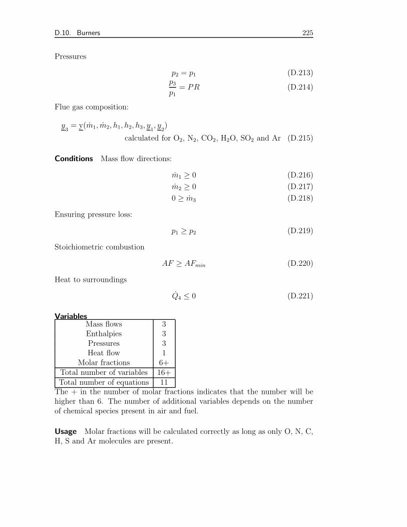
D.10. Burners 225
Pressures
p2 = p1 (D.213)p3
p1= PR (D.214)
Flue gas composition:
y3= y(m1, m2, h1, h2, h3, y1
, y2)
calculated for O2, N2, CO2, H2O, SO2 and Ar (D.215)
Conditions Mass flow directions:
m1 ≥ 0 (D.216)
m2 ≥ 0 (D.217)
0 ≥ m3 (D.218)
Ensuring pressure loss:
p1 ≥ p2 (D.219)
Stoichiometric combustion
AF ≥ AFmin (D.220)
Heat to surroundings
Q4 ≤ 0 (D.221)
VariablesMass flows 3Enthalpies 3Pressures 3Heat flow 1
Molar fractions 6+Total number of variables 16+Total number of equations 11The + in the number of molar fractions indicates that the number will behigher than 6. The number of additional variables depends on the numberof chemical species present in air and fuel.
Usage Molar fractions will be calculated correctly as long as only O, N, C,H, S and Ar molecules are present.
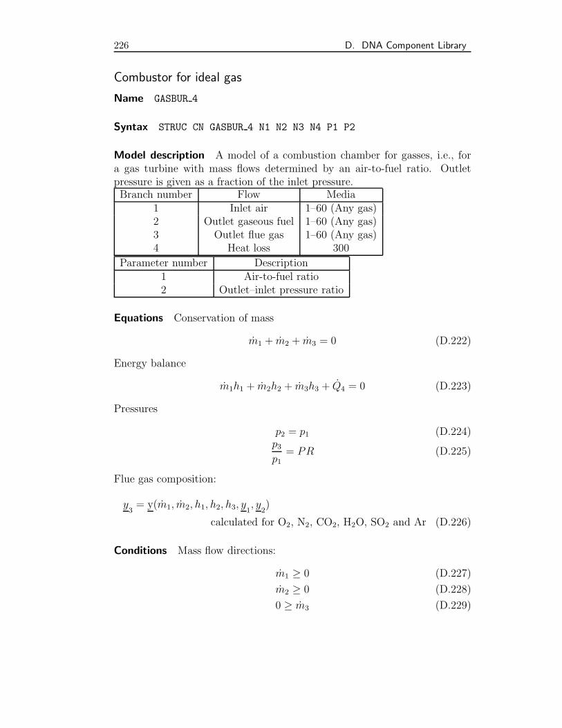
226 D. DNA Component Library
Combustor for ideal gas
Name GASBUR 4
Syntax STRUC CN GASBUR 4 N1 N2 N3 N4 P1 P2
Model description A model of a combustion chamber for gasses, i.e., fora gas turbine with mass flows determined by an air-to-fuel ratio. Outletpressure is given as a fraction of the inlet pressure.Branch number Flow Media
1 Inlet air 1–60 (Any gas)2 Outlet gaseous fuel 1–60 (Any gas)3 Outlet flue gas 1–60 (Any gas)4 Heat loss 300
Parameter number Description1 Air-to-fuel ratio2 Outlet–inlet pressure ratio
Equations Conservation of mass
m1 + m2 + m3 = 0 (D.222)
Energy balance
m1h1 + m2h2 + m3h3 + Q4 = 0 (D.223)
Pressures
p2 = p1 (D.224)p3
p1
= PR (D.225)
Flue gas composition:
y3= y(m1, m2, h1, h2, h3, y1
, y2)
calculated for O2, N2, CO2, H2O, SO2 and Ar (D.226)
Conditions Mass flow directions:
m1 ≥ 0 (D.227)
m2 ≥ 0 (D.228)
0 ≥ m3 (D.229)
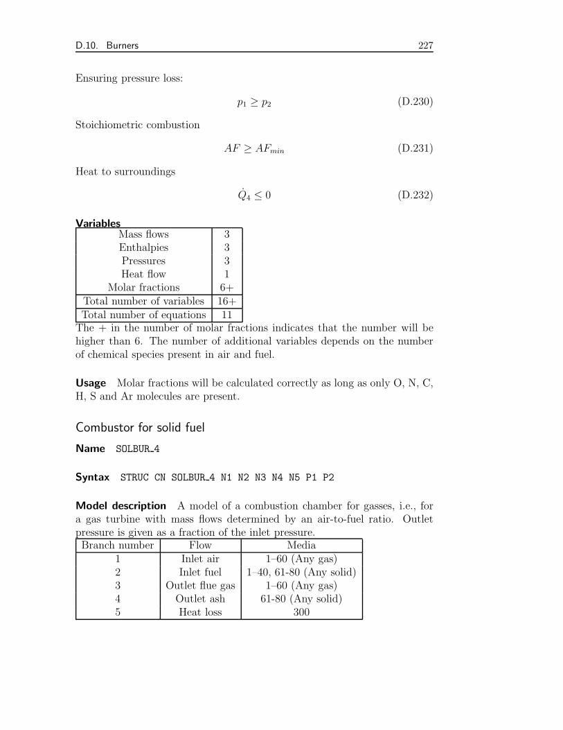
D.10. Burners 227
Ensuring pressure loss:
p1 ≥ p2 (D.230)
Stoichiometric combustion
AF ≥ AFmin (D.231)
Heat to surroundings
Q4 ≤ 0 (D.232)
VariablesMass flows 3Enthalpies 3Pressures 3Heat flow 1
Molar fractions 6+Total number of variables 16+Total number of equations 11The + in the number of molar fractions indicates that the number will behigher than 6. The number of additional variables depends on the numberof chemical species present in air and fuel.
Usage Molar fractions will be calculated correctly as long as only O, N, C,H, S and Ar molecules are present.
Combustor for solid fuel
Name SOLBUR 4
Syntax STRUC CN SOLBUR 4 N1 N2 N3 N4 N5 P1 P2
Model description A model of a combustion chamber for gasses, i.e., fora gas turbine with mass flows determined by an air-to-fuel ratio. Outletpressure is given as a fraction of the inlet pressure.Branch number Flow Media
1 Inlet air 1–60 (Any gas)2 Inlet fuel 1–40, 61-80 (Any solid)3 Outlet flue gas 1–60 (Any gas)4 Outlet ash 61-80 (Any solid)5 Heat loss 300
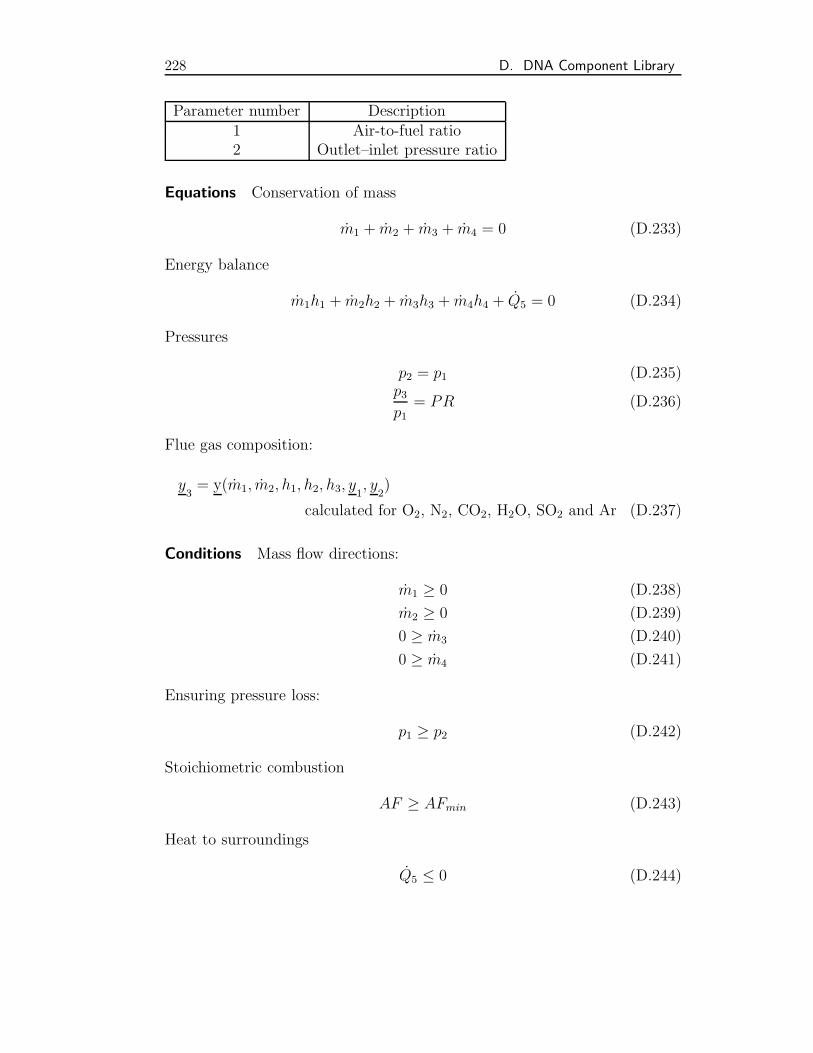
228 D. DNA Component Library
Parameter number Description1 Air-to-fuel ratio2 Outlet–inlet pressure ratio
Equations Conservation of mass
m1 + m2 + m3 + m4 = 0 (D.233)
Energy balance
m1h1 + m2h2 + m3h3 + m4h4 + Q5 = 0 (D.234)
Pressures
p2 = p1 (D.235)p3
p1= PR (D.236)
Flue gas composition:
y3= y(m1, m2, h1, h2, h3, y1
, y2)
calculated for O2, N2, CO2, H2O, SO2 and Ar (D.237)
Conditions Mass flow directions:
m1 ≥ 0 (D.238)
m2 ≥ 0 (D.239)
0 ≥ m3 (D.240)
0 ≥ m4 (D.241)
Ensuring pressure loss:
p1 ≥ p2 (D.242)
Stoichiometric combustion
AF ≥ AFmin (D.243)
Heat to surroundings
Q5 ≤ 0 (D.244)
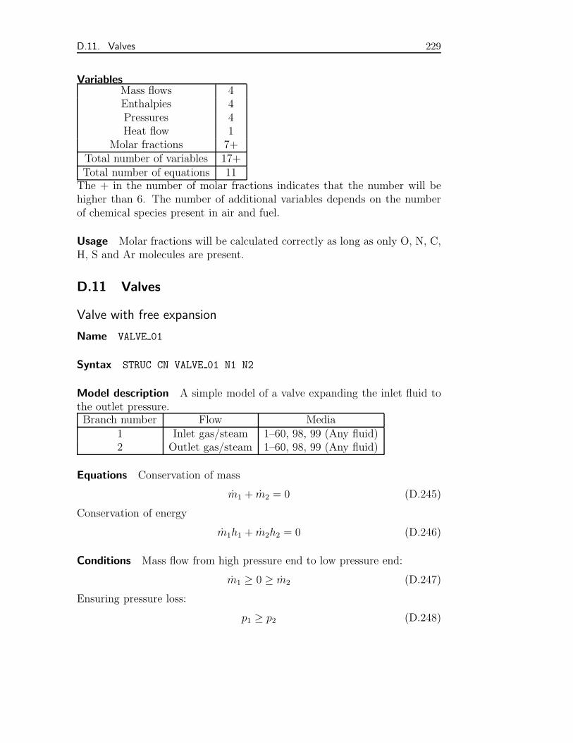
D.11. Valves 229
VariablesMass flows 4Enthalpies 4Pressures 4Heat flow 1
Molar fractions 7+Total number of variables 17+Total number of equations 11The + in the number of molar fractions indicates that the number will behigher than 6. The number of additional variables depends on the numberof chemical species present in air and fuel.
Usage Molar fractions will be calculated correctly as long as only O, N, C,H, S and Ar molecules are present.
D.11 Valves
Valve with free expansion
Name VALVE 01
Syntax STRUC CN VALVE 01 N1 N2
Model description A simple model of a valve expanding the inlet fluid tothe outlet pressure.Branch number Flow Media
1 Inlet gas/steam 1–60, 98, 99 (Any fluid)2 Outlet gas/steam 1–60, 98, 99 (Any fluid)
Equations Conservation of mass
m1 + m2 = 0 (D.245)
Conservation of energy
m1h1 + m2h2 = 0 (D.246)
Conditions Mass flow from high pressure end to low pressure end:
m1 ≥ 0 ≥ m2 (D.247)
Ensuring pressure loss:
p1 ≥ p2 (D.248)
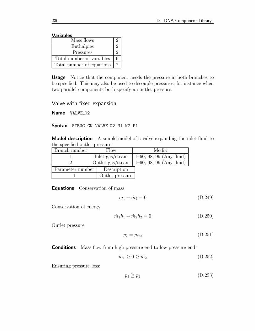
230 D. DNA Component Library
VariablesMass flows 2Enthalpies 2Pressures 2
Total number of variables 6Total number of equations 2
Usage Notice that the component needs the pressure in both branches tobe specified. This may also be used to decouple pressures, for instance whentwo parallel components both specify an outlet pressure.
Valve with fixed expansion
Name VALVE 02
Syntax STRUC CN VALVE 02 N1 N2 P1
Model description A simple model of a valve expanding the inlet fluid tothe specified outlet pressure.Branch number Flow Media
1 Inlet gas/steam 1–60, 98, 99 (Any fluid)2 Outlet gas/steam 1–60, 98, 99 (Any fluid)
Parameter number Description1 Outlet pressure
Equations Conservation of mass
m1 + m2 = 0 (D.249)
Conservation of energy
m1h1 + m2h2 = 0 (D.250)
Outlet pressure
p2 = pout (D.251)
Conditions Mass flow from high pressure end to low pressure end:
m1 ≥ 0 ≥ m2 (D.252)
Ensuring pressure loss:
p1 ≥ p2 (D.253)
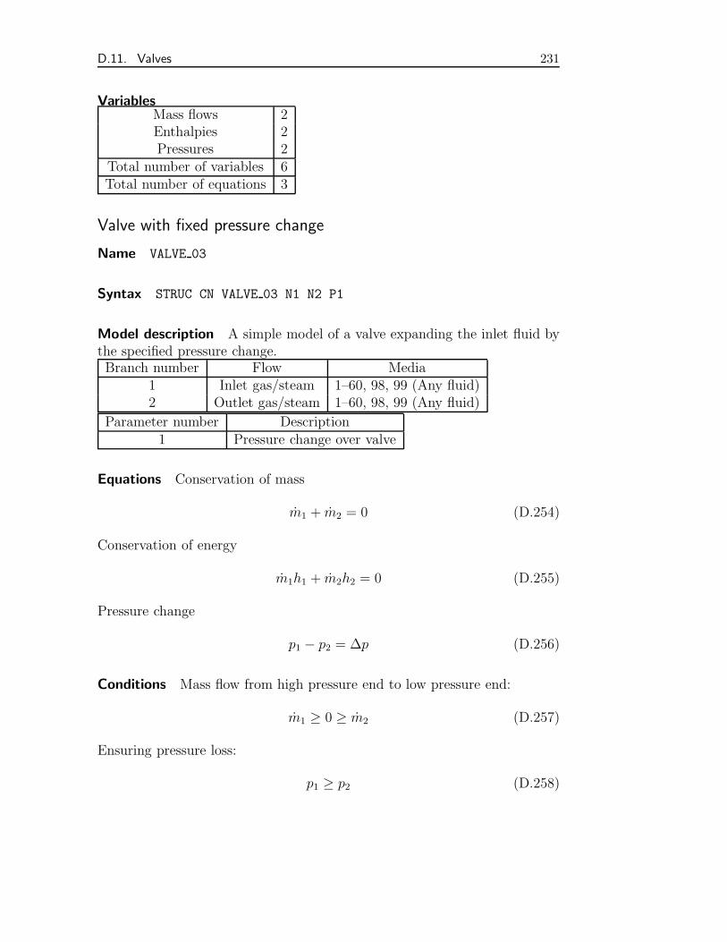
D.11. Valves 231
VariablesMass flows 2Enthalpies 2Pressures 2
Total number of variables 6Total number of equations 3
Valve with fixed pressure change
Name VALVE 03
Syntax STRUC CN VALVE 03 N1 N2 P1
Model description A simple model of a valve expanding the inlet fluid bythe specified pressure change.Branch number Flow Media
1 Inlet gas/steam 1–60, 98, 99 (Any fluid)2 Outlet gas/steam 1–60, 98, 99 (Any fluid)
Parameter number Description1 Pressure change over valve
Equations Conservation of mass
m1 + m2 = 0 (D.254)
Conservation of energy
m1h1 + m2h2 = 0 (D.255)
Pressure change
p1 − p2 = ∆p (D.256)
Conditions Mass flow from high pressure end to low pressure end:
m1 ≥ 0 ≥ m2 (D.257)
Ensuring pressure loss:
p1 ≥ p2 (D.258)
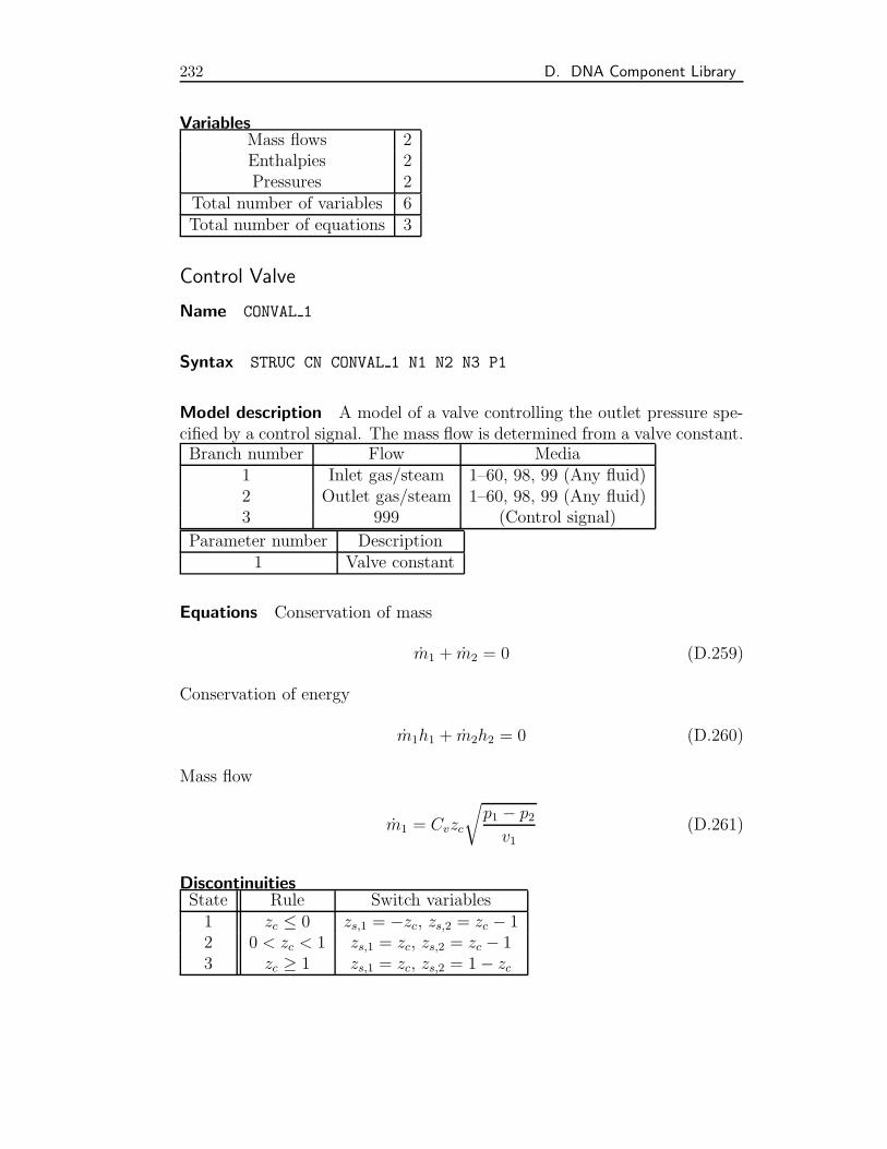
232 D. DNA Component Library
VariablesMass flows 2Enthalpies 2Pressures 2
Total number of variables 6Total number of equations 3
Control Valve
Name CONVAL 1
Syntax STRUC CN CONVAL 1 N1 N2 N3 P1
Model description A model of a valve controlling the outlet pressure spe-cified by a control signal. The mass flow is determined from a valve constant.Branch number Flow Media
1 Inlet gas/steam 1–60, 98, 99 (Any fluid)2 Outlet gas/steam 1–60, 98, 99 (Any fluid)3 999 (Control signal)
Parameter number Description1 Valve constant
Equations Conservation of mass
m1 + m2 = 0 (D.259)
Conservation of energy
m1h1 + m2h2 = 0 (D.260)
Mass flow
m1 = Cvzc
√p1 − p2
v1(D.261)
DiscontinuitiesState Rule Switch variables1 zc ≤ 0 zs,1 = −zc, zs,2 = zc − 12 0 < zc < 1 zs,1 = zc, zs,2 = zc − 13 zc ≥ 1 zs,1 = zc, zs,2 = 1− zc
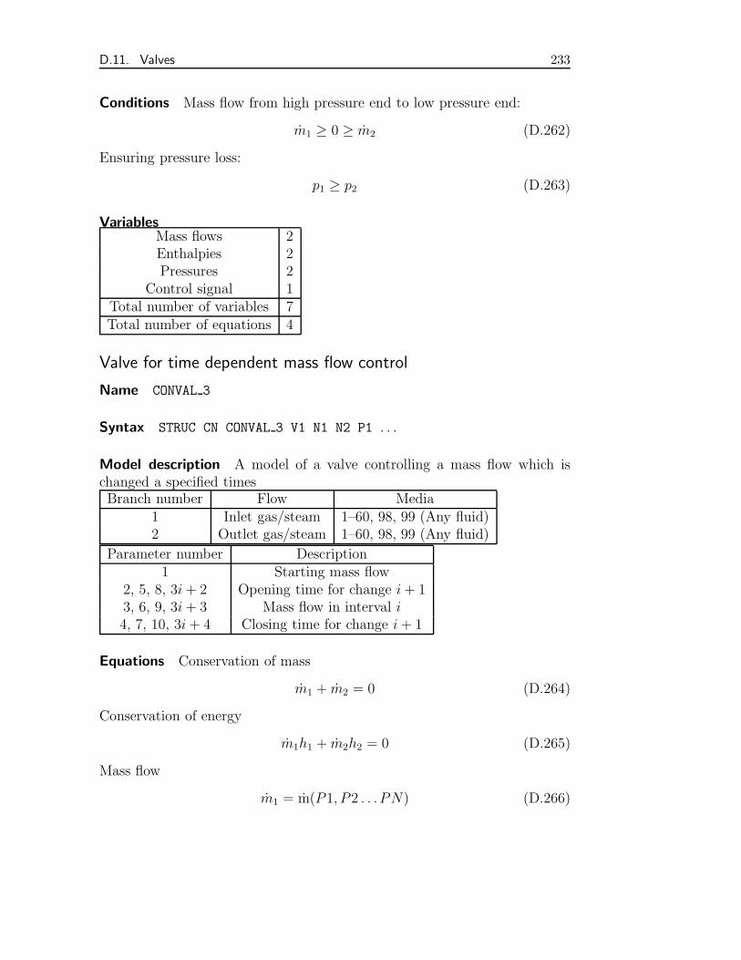
D.11. Valves 233
Conditions Mass flow from high pressure end to low pressure end:
m1 ≥ 0 ≥ m2 (D.262)
Ensuring pressure loss:
p1 ≥ p2 (D.263)
VariablesMass flows 2Enthalpies 2Pressures 2
Control signal 1Total number of variables 7Total number of equations 4
Valve for time dependent mass flow control
Name CONVAL 3
Syntax STRUC CN CONVAL 3 V1 N1 N2 P1 . . .
Model description A model of a valve controlling a mass flow which ischanged a specified timesBranch number Flow Media
1 Inlet gas/steam 1–60, 98, 99 (Any fluid)2 Outlet gas/steam 1–60, 98, 99 (Any fluid)
Parameter number Description1 Starting mass flow
2, 5, 8, 3i+ 2 Opening time for change i+ 13, 6, 9, 3i+ 3 Mass flow in interval i4, 7, 10, 3i+ 4 Closing time for change i+ 1
Equations Conservation of mass
m1 + m2 = 0 (D.264)
Conservation of energy
m1h1 + m2h2 = 0 (D.265)
Mass flow
m1 = m(P1, P2 . . . PN) (D.266)
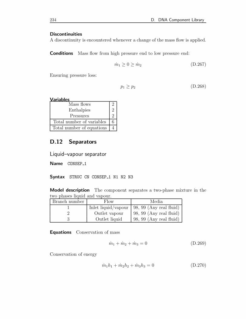
234 D. DNA Component Library
DiscontinuitiesA discontinuity is encountered whenever a change of the mass flow is applied.
Conditions Mass flow from high pressure end to low pressure end:
m1 ≥ 0 ≥ m2 (D.267)
Ensuring pressure loss:
p1 ≥ p2 (D.268)
VariablesMass flows 2Enthalpies 2Pressures 2
Total number of variables 6Total number of equations 4
D.12 Separators
Liquid–vapour separator
Name CONSEP 1
Syntax STRUC CN CONSEP 1 N1 N2 N3
Model description The component separates a two-phase mixture in thetwo phases liquid and vapour.Branch number Flow Media
1 Inlet liquid/vapour 98, 99 (Any real fluid)2 Outlet vapour 98, 99 (Any real fluid)3 Outlet liquid 98, 99 (Any real fluid)
Equations Conservation of mass
m1 + m2 + m3 = 0 (D.269)
Conservation of energy
m1h1 + m2h2 + m3h3 = 0 (D.270)
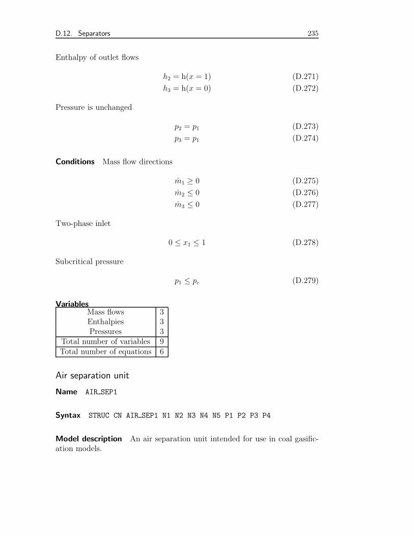
D.12. Separators 235
Enthalpy of outlet flows
h2 = h(x = 1) (D.271)
h3 = h(x = 0) (D.272)
Pressure is unchanged
p2 = p1 (D.273)
p3 = p1 (D.274)
Conditions Mass flow directions
m1 ≥ 0 (D.275)
m2 ≤ 0 (D.276)
m3 ≤ 0 (D.277)
Two-phase inlet
0 ≤ x1 ≤ 1 (D.278)
Subcritical pressure
p1 ≤ pc (D.279)
VariablesMass flows 3Enthalpies 3Pressures 3
Total number of variables 9Total number of equations 6
Air separation unit
Name AIR SEP1
Syntax STRUC CN AIR SEP1 N1 N2 N3 N4 N5 P1 P2 P3 P4
Model description An air separation unit intended for use in coal gasific-ation models.
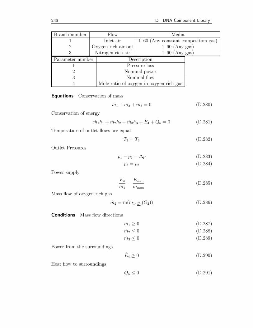
236 D. DNA Component Library
Branch number Flow Media1 Inlet air 1–60 (Any constant composition gas)2 Oxygen rich air out 1–60 (Any gas)3 Nitrogen rich air 1–60 (Any gas)
Parameter number Description1 Pressure loss2 Nominal power3 Nominal flow4 Mole ratio of oxygen in oxygen rich gas
Equations Conservation of mass
m1 + m2 + m3 = 0 (D.280)
Conservation of energy
m1h1 + m2h2 + m3h3 + E4 + Q5 = 0 (D.281)
Temperature of outlet flows are equal
T2 = T3 (D.282)
Outlet Pressures
p1 − p2 = ∆p (D.283)
p3 = p2 (D.284)
Power supply
E4
m1=
Enom
mnom(D.285)
Mass flow of oxygen rich gas
m2 = m(m1, y2(O2)) (D.286)
Conditions Mass flow directions
m1 ≥ 0 (D.287)
m2 ≤ 0 (D.288)
m3 ≤ 0 (D.289)
Power from the surroundings
E4 ≥ 0 (D.290)
Heat flow to surroundings
Q5 ≤ 0 (D.291)
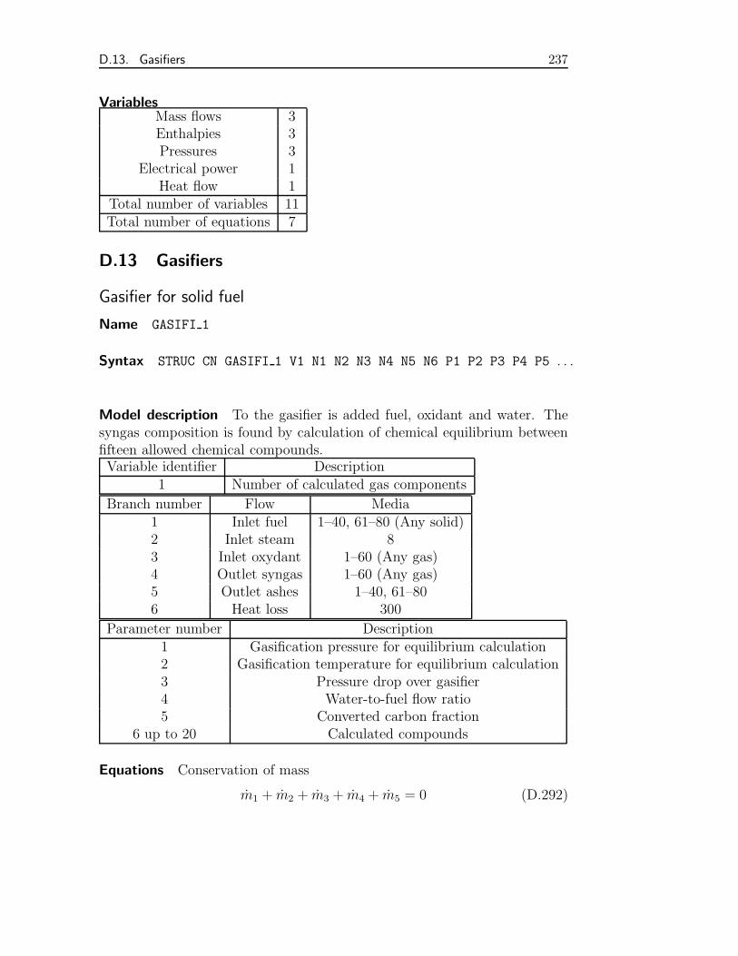
D.13. Gasifiers 237
VariablesMass flows 3Enthalpies 3Pressures 3
Electrical power 1Heat flow 1
Total number of variables 11Total number of equations 7
D.13 Gasifiers
Gasifier for solid fuel
Name GASIFI 1
Syntax STRUC CN GASIFI 1 V1 N1 N2 N3 N4 N5 N6 P1 P2 P3 P4 P5 . . .
Model description To the gasifier is added fuel, oxidant and water. Thesyngas composition is found by calculation of chemical equilibrium betweenfifteen allowed chemical compounds.Variable identifier Description
1 Number of calculated gas components
Branch number Flow Media1 Inlet fuel 1–40, 61–80 (Any solid)2 Inlet steam 83 Inlet oxydant 1–60 (Any gas)4 Outlet syngas 1–60 (Any gas)5 Outlet ashes 1–40, 61–806 Heat loss 300
Parameter number Description1 Gasification pressure for equilibrium calculation2 Gasification temperature for equilibrium calculation3 Pressure drop over gasifier4 Water-to-fuel flow ratio5 Converted carbon fraction
6 up to 20 Calculated compounds
Equations Conservation of mass
m1 + m2 + m3 + m4 + m5 = 0 (D.292)
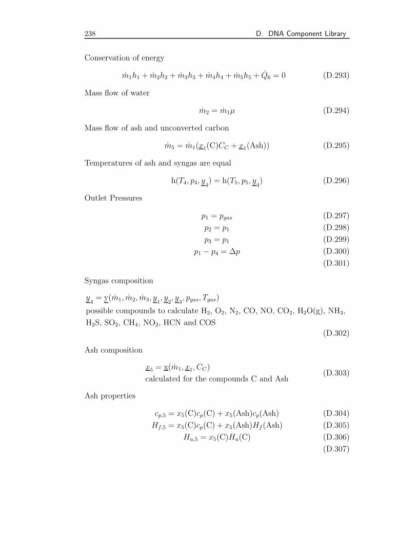
238 D. DNA Component Library
Conservation of energy
m1h1 + m2h2 + m3h3 + m4h4 + m5h5 + Q6 = 0 (D.293)
Mass flow of water
m2 = m1µ (D.294)
Mass flow of ash and unconverted carbon
m5 = m1(x1(C)CC + x1(Ash)) (D.295)
Temperatures of ash and syngas are equal
h(T4, p4, y4) = h(T5, p5, y4
) (D.296)
Outlet Pressures
p1 = pgas (D.297)
p2 = p1 (D.298)
p3 = p1 (D.299)
p1 − p4 = ∆p (D.300)
(D.301)
Syngas composition
y4= y(m1, m2, m3, y1
, y2, y
3, pgas, Tgas)
possible compounds to calculate H2, O2, N2, CO, NO, CO2, H2O(g), NH3,
H2S, SO2, CH4, NO2, HCN and COS
(D.302)
Ash composition
x5 = x(m1, x1, CC)
calculated for the compounds C and Ash(D.303)
Ash properties
cp,5 = x5(C)cp(C) + x5(Ash)cp(Ash) (D.304)
Hf,5 = x5(C)cp(C) + x5(Ash)Hf(Ash) (D.305)
Hu,5 = x5(C)Hu(C) (D.306)
(D.307)
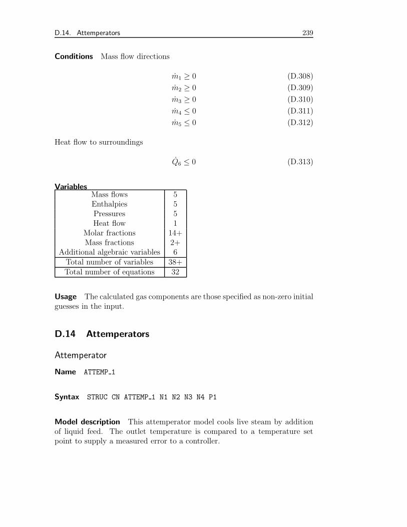
D.14. Attemperators 239
Conditions Mass flow directions
m1 ≥ 0 (D.308)
m2 ≥ 0 (D.309)
m3 ≥ 0 (D.310)
m4 ≤ 0 (D.311)
m5 ≤ 0 (D.312)
Heat flow to surroundings
Q6 ≤ 0 (D.313)
VariablesMass flows 5Enthalpies 5Pressures 5Heat flow 1
Molar fractions 14+Mass fractions 2+
Additional algebraic variables 6Total number of variables 38+Total number of equations 32
Usage The calculated gas components are those specified as non-zero initialguesses in the input.
D.14 Attemperators
Attemperator
Name ATTEMP 1
Syntax STRUC CN ATTEMP 1 N1 N2 N3 N4 P1
Model description This attemperator model cools live steam by additionof liquid feed. The outlet temperature is compared to a temperature setpoint to supply a measured error to a controller.
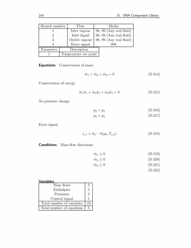
240 D. DNA Component Library
Branch number Flow Media1 Inlet vapour 98, 99 (Any real fluid)2 Inlet liquid 98, 99 (Any real fluid)3 Outlet vapour 98, 99 (Any real fluid)4 Error signal 999
Parameter Description1 Temperature set point
Equations Conservation of mass
m1 + m2 + m3 = 0 (D.314)
Conservation of energy
m1h1 + m2h2 + m3h3 = 0 (D.315)
No pressure change
p2 = p1 (D.316)
p3 = p1 (D.317)
Error signal
zc,1 = h3 − h(p3, Tref) (D.318)
Conditions Mass flow directions:
m1 ≥ 0 (D.319)
m2 ≥ 0 (D.320)
m3 ≤ 0 (D.321)
(D.322)
VariablesMass flows 3Enthalpies 3Pressures 3
Control signal 1Total number of variables 10Total number of equations 5
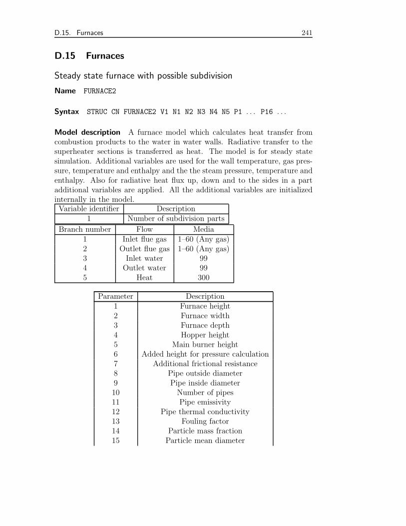
D.15. Furnaces 241
D.15 Furnaces
Steady state furnace with possible subdivision
Name FURNACE2
Syntax STRUC CN FURNACE2 V1 N1 N2 N3 N4 N5 P1 . . . P16 . . .
Model description A furnace model which calculates heat transfer fromcombustion products to the water in water walls. Radiative transfer to thesuperheater sections is transferred as heat. The model is for steady statesimulation. Additional variables are used for the wall temperature, gas pres-sure, temperature and enthalpy and the the steam pressure, temperature andenthalpy. Also for radiative heat flux up, down and to the sides in a partadditional variables are applied. All the additional variables are initializedinternally in the model.Variable identifier Description
1 Number of subdivision parts
Branch number Flow Media1 Inlet flue gas 1–60 (Any gas)2 Outlet flue gas 1–60 (Any gas)3 Inlet water 994 Outlet water 995 Heat 300
Parameter Description1 Furnace height2 Furnace width3 Furnace depth4 Hopper height5 Main burner height6 Added height for pressure calculation7 Additional frictional resistance8 Pipe outside diameter9 Pipe inside diameter10 Number of pipes11 Pipe emissivity12 Pipe thermal conductivity13 Fouling factor14 Particle mass fraction15 Particle mean diameter
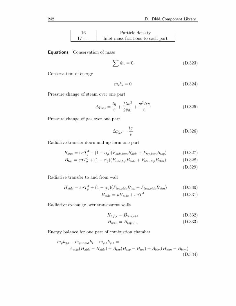
242 D. DNA Component Library
16 Particle density17 . . . Inlet mass fractions to each part
Equations Conservation of mass∑mi = 0 (D.323)
Conservation of energy
mihi = 0 (D.324)
Pressure change of steam over one part
∆pw,i =lg
v+flw2
2vdi+w2∆v
v(D.325)
Pressure change of gas over one part
∆pg,i =lg
v(D.326)
Radiative transfer down and up form one part
Bbtm = εσT 4g + (1− αg)(Fside,btmBside + Ftop,btmBtop) (D.327)
Btop = εσT 4g + (1− αg)(Fside,topBside + Fbtm,topBbtm) (D.328)
(D.329)
Radiative transfer to and from wall
Hside = εσT 4g + (1− αg)(Ftop,sideBtop + Fbtm,sideBbtm) (D.330)
Bside = ρHside + εσT 4 (D.331)
Radiative exchange over transparent walls
Htop,i = Bbtm,i+1 (D.332)
Hbot,i = Btop,i−1 (D.333)
Energy balance for one part of combustion chamber
mghg,i + mg,inputhi − mg,ohg,o =
Aside(Hside − Bside) + Atop(Htop −Btop) + Abtm(Hbtm − Bbtm)
(D.334)
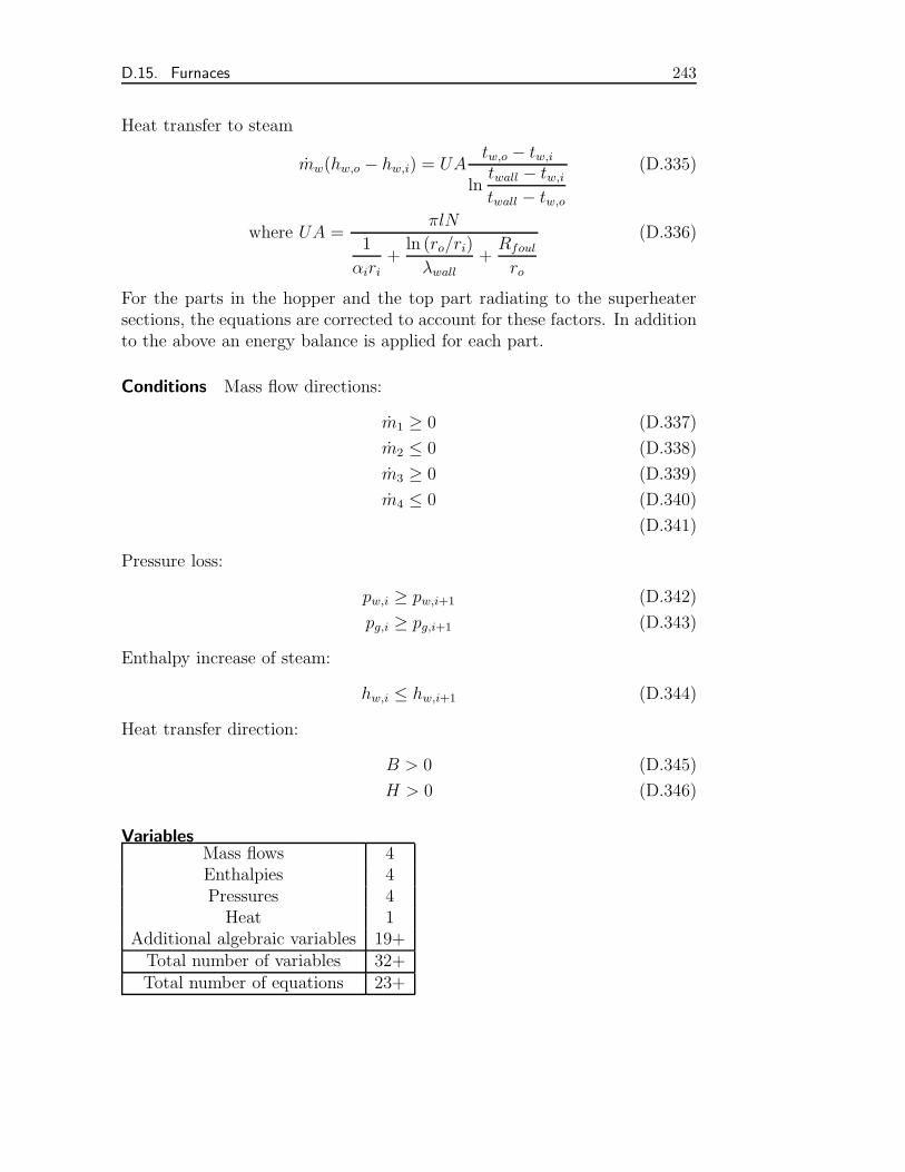
D.15. Furnaces 243
Heat transfer to steam
mw(hw,o − hw,i) = UAtw,o − tw,i
lntwall − tw,itwall − tw,o
(D.335)
where UA =πlN
1
αiri+ln (ro/ri)
λwall+Rfoul
ro
(D.336)
For the parts in the hopper and the top part radiating to the superheatersections, the equations are corrected to account for these factors. In additionto the above an energy balance is applied for each part.
Conditions Mass flow directions:
m1 ≥ 0 (D.337)
m2 ≤ 0 (D.338)
m3 ≥ 0 (D.339)
m4 ≤ 0 (D.340)
(D.341)
Pressure loss:
pw,i ≥ pw,i+1 (D.342)
pg,i ≥ pg,i+1 (D.343)
Enthalpy increase of steam:
hw,i ≤ hw,i+1 (D.344)
Heat transfer direction:
B > 0 (D.345)
H > 0 (D.346)
VariablesMass flows 4Enthalpies 4Pressures 4Heat 1
Additional algebraic variables 19+Total number of variables 32+Total number of equations 23+
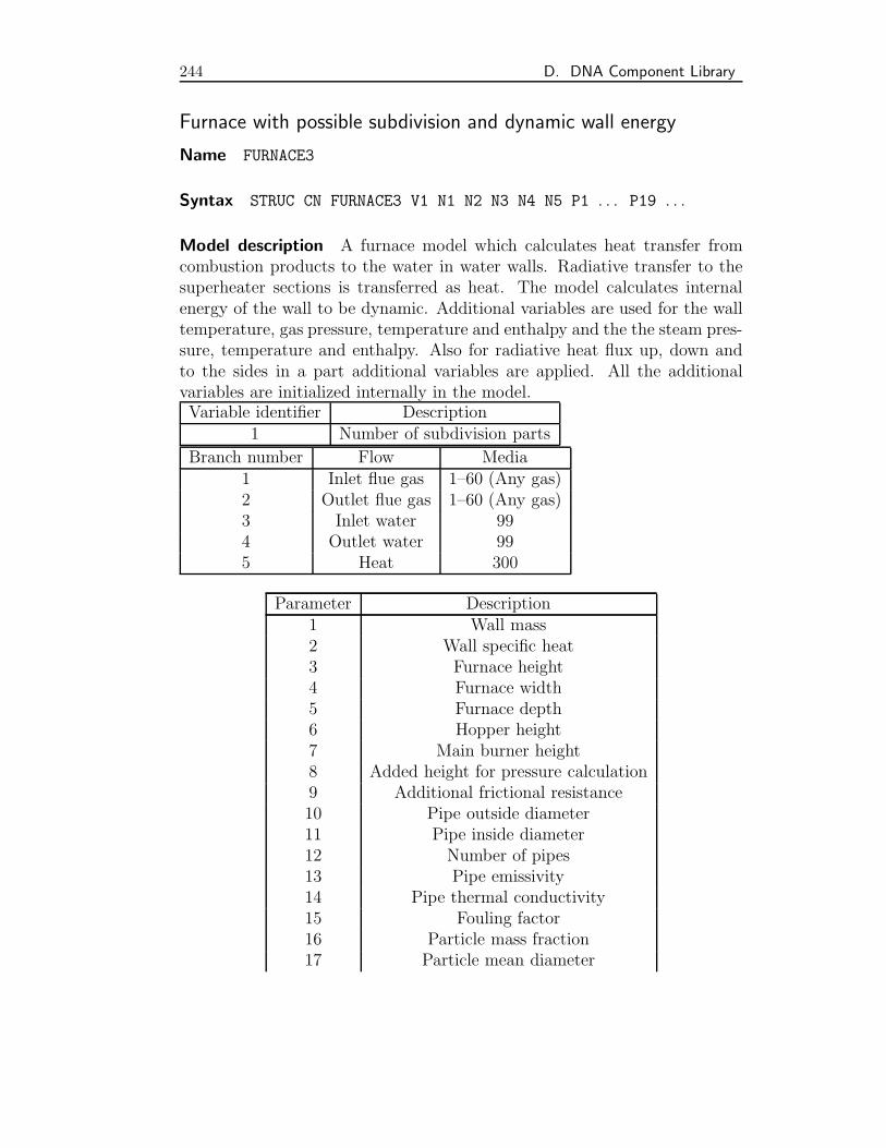
244 D. DNA Component Library
Furnace with possible subdivision and dynamic wall energy
Name FURNACE3
Syntax STRUC CN FURNACE3 V1 N1 N2 N3 N4 N5 P1 . . . P19 . . .
Model description A furnace model which calculates heat transfer fromcombustion products to the water in water walls. Radiative transfer to thesuperheater sections is transferred as heat. The model calculates internalenergy of the wall to be dynamic. Additional variables are used for the walltemperature, gas pressure, temperature and enthalpy and the the steam pres-sure, temperature and enthalpy. Also for radiative heat flux up, down andto the sides in a part additional variables are applied. All the additionalvariables are initialized internally in the model.Variable identifier Description
1 Number of subdivision parts
Branch number Flow Media1 Inlet flue gas 1–60 (Any gas)2 Outlet flue gas 1–60 (Any gas)3 Inlet water 994 Outlet water 995 Heat 300
Parameter Description1 Wall mass2 Wall specific heat3 Furnace height4 Furnace width5 Furnace depth6 Hopper height7 Main burner height8 Added height for pressure calculation9 Additional frictional resistance10 Pipe outside diameter11 Pipe inside diameter12 Number of pipes13 Pipe emissivity14 Pipe thermal conductivity15 Fouling factor16 Particle mass fraction17 Particle mean diameter
D.15. Furnaces 245
18 Particle density19 . . . Inlet mass fractions to each part
Equations Conservation of mass∑mi = 0 (D.347)
Conservation of energy
mihi =dUs
dτ(D.348)
Pressure change of steam over one part
∆pw,i =lg
v+flw2
2vdi+w2∆v
v(D.349)
Pressure change of gas over one part
∆pg,i =lg
v(D.350)
Radiative transfer down and up form one part
Bbtm = εσT 4g + (1− αg)(Fside,btmBside + Ftop,btmBtop) (D.351)
Btop = εσT 4g + (1− αg)(Fside,topBside + Fbtm,topBbtm) (D.352)
(D.353)
Radiative transfer to and from wall
Hside = εσT 4g + (1− αg)(Ftop,sideBtop + Fbtm,sideBbtm) (D.354)
Bside = ρHside + εσT 4 (D.355)
Radiative exchange over transparent walls
Htop,i = Bbtm,i+1 (D.356)
Hbot,i = Btop,i−1 (D.357)
Energy balance for one part of combustion chamber
mghg,i + mg,inputhi − mg,ohg,o =
Aside(Hside −Bside) + Atop(Htop −Btop) + Abtm(Hbtm − Bbtm)
(D.358)
246 D. DNA Component Library
Heat transfer to steam
mw(hw,o − hw,i) = UAtw,o − tw,i
lntwall − tw,itwall − tw,o
(D.359)
where UA =πlN
1
αiri+ln (ro/ri)
λwall+Rfoul
ro
(D.360)
For the parts in the hopper and the top part radiating to the superheatersections, the equations are corrected to account for these factors. In additionto the above an energy balance is applied for each part.
Conditions Mass flow directions:
m1 ≥ 0 (D.361)
m2 ≤ 0 (D.362)
m3 ≥ 0 (D.363)
m4 ≤ 0 (D.364)
(D.365)
Pressure loss:
pw,i ≥ pw,i+1 (D.366)
pg,i ≥ pg,i+1 (D.367)
Enthalpy increase of steam:
hw,i ≤ hw,i+1 (D.368)
Heat transfer direction:
B > 0 (D.369)
H > 0 (D.370)
VariablesMass flows 4Enthalpies 4Pressures 4Heat 1
Wall energy 3Additional algebraic variables 19+Total number of variables 35+Total number of equations 23+
D.16. Superheaters 247
D.16 Superheaters
Crossflow tube bundle Superheater for steady state
Name XHEATEX2
Syntax STRUC CN XHEATEX2 V1 N1 N2 N3 N4 N5 P1 . . . P16
Model description A model of a cross flow heat exchanger for use as asuperheater. The model handles both radiative and convective heat transfer.The heat exchange is governed by a heat transfer coefficient and a surfacearea. A pressure loss may be applied to the fluid flows.Variable identifier Description
1 Number of passes
Branch number Flow Media1 Inlet gas 1–602 Outlet gas 1–603 Inlet steam 994 Outlet steam 995 Heat loss 300
Parameter number Description1 Pipe outside diameter2 Pipe inside diameter3 Transversal pitch4 Longitudinal pitch5 Number of rows6 Number of tubes pr. row7 Channel width8 Channel depth9 Pipe wall emissivity10 Pipe wall conductivity11 Fouling12 Gas particle mass fraction13 Gas particle mean diameter14 Gas particle density15 Flow configuration16 Additional frictional pressure loss
248 D. DNA Component Library
Equations Conservation of mass
m1 + m2 = 0 (D.371)
m3 + m4 = 0 (D.372)
Energy balance
m1h1 + m2h2 + m3h3 + m4h4 + Q5 = 0 (D.373)
Heat transfer relation for one pass
m1h1 + m2h2 =
FTUA(T1 − T4)− (T2 − T3)
lnT1 − T4
T2 − T3
, for mIcp,I = mIIcp,II
FTUA(T1 − T4), for mIcp,I = mIIcp,II(D.374)
The is heat transfer is found as:
UA =2πLN
1
αiri+ln (ro/ri)
λwall+Rfoul
ro+
1
(αrad + αo)ro
(D.375)
Convective heat transfer is a function of Reynolds and Prandtl numbers.Radiative transfer is found in the gas volume by calculation of the radiativeproperties of the flue gas.
Pressure loss over one pass
p1 − p2 = NRgSL + fw2S2
T v
2(ST − do)(D.376)
p3 − p4 =flw2
2vdi+w2∆v
v(D.377)
Conditions Mass flow directions:
m1 ≥ 0 ≥ m2 (D.378)
m3 ≥ 0 ≥ m4 (D.379)
Ensuring pressure loss:
p1 ≥ p2 (D.380)
p3 ≥ p4 (D.381)
D.16. Superheaters 249
Hot flow is cooled:
T1 ≥ T2 (D.382)
No cross of temperature profiles:
T1 ≥ T4 (D.383)
T2 ≥ T3 (D.384)
VariablesMass flows 4Enthalpies 4Pressures 4Heat 1
Additional Algebraic variables 0+Total number of variables 13+Total number of equations 6+
Usage It is assumed that heat is transferred from side I to side II, so acondition is violated if side II inlet temperature is higher than side I inlettemperature. The heat transfer equation (D.374) is undefined if the tem-perature values supplied make the temperature profiles cross. The modelhandles this situation by applying a zero temperature difference at the end,where the temperatures are closest.
Finned Crossflow tube bundle Superheater for steady state
Name XHEATEX3
Syntax STRUC CN XHEATEX3 V1 N1 N2 N3 N4 N5 P1 . . . P20
Model description A model of a finned cross flow heat exchanger for useas a superheater. The model handles both radiative and convective heattransfer. The heat exchange is governed by a heat transfer coefficient and asurface area. A pressure loss may be applied to the fluid flows.Variable identifier Description
1 Number of passes
250 D. DNA Component Library
Branch number Flow Media1 Inlet gas 1–602 Outlet gas 1–603 Inlet steam 994 Outlet steam 995 Heat loss 300
Parameter number Description1 Pipe outside diameter2 Pipe inside diameter3 Transversal pitch4 Longitudinal pitch5 Number of rows6 Number of tubes pr. row7 Channel width8 Channel depth9 Pipe wall emissivity10 Pipe wall conductivity11 Fin diameter12 Fin width13 Fin pitch14 Fin thermal conductivity15 Fouling16 Gas particle mass fraction17 Gas particle mean diameter18 Gas particle density19 Flow configuration20 Additional frictional pressure loss
Equations Conservation of mass
m1 + m2 = 0 (D.385)
m3 + m4 = 0 (D.386)
Energy balance
m1h1 + m2h2 + m3h3 + m4h4 + Q5 = 0 (D.387)
D.16. Superheaters 251
Heat transfer relation for one pass
m1h1 + m2h2 =
FTUA(T1 − T4)− (T2 − T3)
lnT1 − T4
T2 − T3
, for mIcp,I = mIIcp,II
FTUA(T1 − T4), for mIcp,I = mIIcp,II(D.388)
The is heat transfer is found as:
UA =2πLN
1
αiri+ln (ro/ri)
λwall+Rfoul
ro+
1
(αrad + αo)ro
(D.389)
Convective heat transfer is a function of Reynolds and Prandtl numbers. Theoutside transfer coefficient is corrected to account for fins. Radiative transferis found in the gas volume by calculation of the radiative properties of theflue gas.
Pressure loss over one pass
p1 − p2 = NRgSL + fw2S2
T v
2(ST − do)(D.390)
p3 − p4 =flw2
2vdi+w2∆v
v(D.391)
Conditions Mass flow directions:
m1 ≥ 0 ≥ m2 (D.392)
m3 ≥ 0 ≥ m4 (D.393)
Ensuring pressure loss:
p1 ≥ p2 (D.394)
p3 ≥ p4 (D.395)
Hot flow is cooled:
T1 ≥ T2 (D.396)
No cross of temperature profiles:
T1 ≥ T4 (D.397)
T2 ≥ T3 (D.398)
252 D. DNA Component Library
VariablesMass flows 4Enthalpies 4Pressures 4Heat 1
Additional Algebraic variables 0+Total number of variables 13+Total number of equations 6+
Usage It is assumed that heat is transferred from side I to side II, so acondition is violated if side II inlet temperature is higher than side I inlettemperature. The heat transfer equation (D.388) is undefined if the tem-perature values supplied make the temperature profiles cross. The modelhandles this situation by applying a zero temperature difference at the end,where the temperatures are closest.
Crossflow tube bundle Superheater with dynamic wall energy
Name XHEATEX4
Syntax STRUC CN XHEATEX4 V1 N1 N2 N3 N4 N5 P1 . . . P16
Model description A model of a cross flow heat exchanger for use as asuperheater. The model handles both radiative and convective heat transfer.The heat exchange is governed by a heat transfer coefficient and a surfacearea. A pressure loss may be applied to the fluid flows.Variable identifier Description
1 Number of passes
Branch number Flow Media1 Inlet gas 1–602 Outlet gas 1–603 Inlet steam 994 Outlet steam 995 Heat loss 300
Parameter number Description1 Wall mass2 Specific heat of wall3 Pipe outside diameter4 Pipe inside diameter
D.16. Superheaters 253
5 Transversal pitch6 Longitudinal pitch7 Number of rows8 Number of tubes pr. row9 Channel width10 Channel depth11 Pipe wall emissivity12 Pipe wall conductivity13 Fouling14 Gas particle mass fraction15 Gas particle mean diameter16 Gas particle density17 Flow configuration18 Additional frictional pressure loss
Equations Conservation of mass
m1 + m2 = 0 (D.399)
m3 + m4 = 0 (D.400)
Energy balance
m1h1 + m2h2 + m3h3 + m4h4 + Q5 =dUS
dτ(D.401)
Heat transfer relation for one pass
m1h1 + m2h2 =
FTUA(T1 − T4)− (T2 − T3)
lnT1 − T4
T2 − T3
, for mIcp,I = mIIcp,II
FTUA(T1 − T4), for mIcp,I = mIIcp,II(D.402)
The is heat transfer is found as:
UA =2πLN
1
αiri+ln (ro/ri)
λwall+Rfoul
ro+
1
(αrad + αo)ro
(D.403)
Convective heat transfer is a function of Reynolds and Prandtl numbers.Radiative transfer is found in the gas volume by calculation of the radiativeproperties of the flue gas.
254 D. DNA Component Library
Pressure loss over one pass
p1 − p2 = NRgSL + fw2S2
T v
2(ST − do)(D.404)
p3 − p4 =flw2
2vdi+w2∆v
v(D.405)
Conditions Mass flow directions:
m1 ≥ 0 ≥ m2 (D.406)
m3 ≥ 0 ≥ m4 (D.407)
Ensuring pressure loss:
p1 ≥ p2 (D.408)
p3 ≥ p4 (D.409)
Hot flow is cooled:
T1 ≥ T2 (D.410)
No cross of temperature profiles:
T1 ≥ T4 (D.411)
T2 ≥ T3 (D.412)
VariablesMass flows 4Enthalpies 4Pressures 4Heat 1
Wall energy 3Additional Algebraic variables 0+Total number of variables 16+Total number of equations 6+
Usage It is assumed that heat is transferred from side I to side II, so acondition is violated if side II inlet temperature is higher than side I inlettemperature. The heat transfer equation (D.402) is undefined if the tem-perature values supplied make the temperature profiles cross. The modelhandles this situation by applying a zero temperature difference at the end,where the temperatures are closest.
D.16. Superheaters 255
Finned Crossflow tube bundle Superheater with dynamic wallenergy
Name XHEATEX5
Syntax STRUC CN XHEATEX3 V1 N1 N2 N3 N4 N5 P1 . . . P22
Model description A model of a finned cross flow heat exchanger for useas a superheater. The model handles both radiative and convective heattransfer. The heat exchange is governed by a heat transfer coefficient and asurface area. A pressure loss may be applied to the fluid flows.Variable identifier Description
1 Number of passes
Branch number Flow Media1 Inlet gas 1–602 Outlet gas 1–603 Inlet steam 994 Outlet steam 995 Heat loss 300
Parameter number Description1 Wall mass2 Wall specific energy3 Pipe outside diameter4 Pipe inside diameter5 Transversal pitch6 Longitudinal pitch7 Number of rows8 Number of tubes pr. row9 Channel width10 Channel depth11 Pipe wall emissivity12 Pipe wall conductivity13 Fin diameter14 Fin width15 Fin pitch16 Fin thermal conductivity17 Fouling18 Gas particle mass fraction19 Gas particle mean diameter20 Gas particle density
256 D. DNA Component Library
21 Flow configuration22 Additional frictional pressure loss
Equations Conservation of mass
m1 + m2 = 0 (D.413)
m3 + m4 = 0 (D.414)
Energy balance
m1h1 + m2h2 + m3h3 + m4h4 + Q5 =dUS
dτ(D.415)
Heat transfer relation for one pass
m1h1 + m2h2 =
FTUA(T1 − T4)− (T2 − T3)
lnT1 − T4
T2 − T3
, for mIcp,I = mIIcp,II
FTUA(T1 − T4), for mIcp,I = mIIcp,II(D.416)
The is heat transfer is found as:
UA =2πLN
1
αiri+ln (ro/ri)
λwall+Rfoul
ro+
1
(αrad + αo)ro
(D.417)
Convective heat transfer is a function of Reynolds and Prandtl numbers. Theoutside transfer coefficient is corrected to account for fins. Radiative transferis found in the gas volume by calculation of the radiative properties of theflue gas.
Pressure loss over one pass
p1 − p2 = NRgSL + fw2S2
T v
2(ST − do)(D.418)
p3 − p4 =flw2
2vdi+w2∆v
v(D.419)
Conditions Mass flow directions:
m1 ≥ 0 ≥ m2 (D.420)
m3 ≥ 0 ≥ m4 (D.421)
D.17. Ducts with heat loss and dynamic effects 257
Ensuring pressure loss:
p1 ≥ p2 (D.422)
p3 ≥ p4 (D.423)
Hot flow is cooled:
T1 ≥ T2 (D.424)
No cross of temperature profiles:
T1 ≥ T4 (D.425)
T2 ≥ T3 (D.426)
VariablesMass flows 4Enthalpies 4Pressures 4Heat 1
Wall energy 3Additional Algebraic variables 0+Total number of variables 16+Total number of equations 6+
Usage It is assumed that heat is transferred from side I to side II, so acondition is violated if side II inlet temperature is higher than side I inlettemperature. The heat transfer equation (D.416) is undefined if the tem-perature values supplied make the temperature profiles cross. The modelhandles this situation by applying a zero temperature difference at the end,where the temperatures are closest.
D.17 Ducts with heat loss and dynamic effects
Duct with heat loss and dynamic energy of solid wall
Name HEATDUC 0
Syntax STRUC CN HEATDUC 0 N1 N2 P1 P2 P3 P4 P5
258 D. DNA Component Library
Model description Duct model with the internal energy of the solid as adifferential variable. Heat transfer calculation is based on an overall heattransfer coefficient. Pressure loss is mass flow dependent.Branch number Flow Media
1 Inlet fluid 1–60, 98, 99 (Any fluid)2 Outlet fluid 1–60, 98, 99 (Any fluid)
Parameter Description1 Solid wall mass2 Solid wall specific heat3 Heat transfer coefficient4 Surface area5 Pressure loss coefficient
Equations Conservation of mass
m1 + m2 = 0 (D.427)
Conservation of energy
m1h1 + m2h2 =dUs
dτ(D.428)
Heat transfer
m1h1 + m2h2 = UA(T1 − TS)− (T2 − TS)
lnT1 − TST2 − TS
with the wall temperature given by Us =MscsTs
(D.429)
Pressure loss
p1 − p2 = fp
(m1 − m2
2
)2
(D.430)
Conditions Mass flow directions
m1 ≥ 0 (D.431)
m2 ≤ 0 (D.432)
The fluid is warmer than the wall and is cooled
T1 ≥ T2 > Ts (D.433)
D.17. Ducts with heat loss and dynamic effects 259
VariablesMass flows 2Enthalpies 2Pressures 2
Solid energy 1Total number of variables 7Total number of equations 4
Duct with heat loss and dynamic energy of fluid and solid wall
Name HEATDUC 1
Syntax STRUC CN HEATDUC 1 N1 N2 P1 P2 P3 P4 P5 P6
Model description Duct model with the internal energy of the fluid andthe solid as differential variables. Heat transfer calculation is based on anoverall heat transfer coefficient. Pressure loss is mass flow dependent.Branch number Flow Media
1 Inlet fluid 1–60, 98, 99 (Any fluid)2 Outlet fluid 1–60, 98, 99 (Any fluid)
Parameter Description1 Fluid mass2 Solid wall mass3 Solid wall specific heat4 Heat transfer coefficient5 Surface area6 Pressure loss coefficient
Equations Conservation of mass
m1 + m2 = 0 (D.434)
Conservation of energy
m1h1 + m2h2 =dUs
dτ+dUI
dτ(D.435)
Heat transfer
m1h1 + m2h2 − dUI
dτ= UA
(T1 − TS)− (T2 − TS)
lnT1 − TST2 − TS
with the wall temperature given by Us =MscsTs
(D.436)
260 D. DNA Component Library
Fluid internal energy
UI =MIu1 + u2
2(D.437)
Pressure loss
p1 − p2 = fp
(m1 − m2
2
)2
(D.438)
Conditions Mass flow directions
m1 ≥ 0 (D.439)
m2 ≤ 0 (D.440)
The fluid is warmer than the wall and is cooled
T1 ≥ T2 > Ts (D.441)
VariablesMass flows 2Enthalpies 2Pressures 2
Fluid energy 1Solid energy 1
Total number of variables 8Total number of equations 5
Duct with heat loss, dynamic fluid mass and dynamic energy offluid and solid wall
Name HEATDUC 2
Syntax STRUC CN HEATDUC 2 N1 N2 P1 P2 P3 P4 P5 P6
Model description Duct model with the mass and internal energy of thefluid and the energy of the solid as differential variables. Heat transfer cal-culation is based on an overall heat transfer coefficient. Pressure loss is massflow dependent.
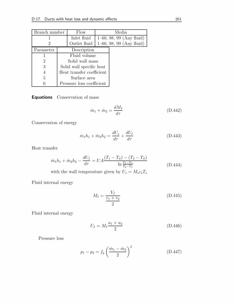
D.17. Ducts with heat loss and dynamic effects 261
Branch number Flow Media1 Inlet fluid 1–60, 98, 99 (Any fluid)2 Outlet fluid 1–60, 98, 99 (Any fluid)
Parameter Description1 Fluid volume2 Solid wall mass3 Solid wall specific heat4 Heat transfer coefficient5 Surface area6 Pressure loss coefficient
Equations Conservation of mass
m1 + m2 =dMI
dτ(D.442)
Conservation of energy
m1h1 + m2h2 =dUs
dτ+dUI
dτ(D.443)
Heat transfer
m1h1 + m2h2 − dUI
dτ= UA
(T1 − TS)− (T2 − TS)
ln T1−TS
T2−TS
with the wall temperature given by Us =MscsTs
(D.444)
Fluid internal energy
MI =VI
v1 + v2
2
(D.445)
Fluid internal energy
UI = MIu1 + u2
2(D.446)
Pressure loss
p1 − p2 = fp
(m1 − m2
2
)2
(D.447)
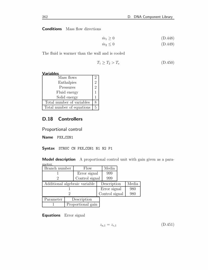
262 D. DNA Component Library
Conditions Mass flow directions
m1 ≥ 0 (D.448)
m2 ≤ 0 (D.449)
The fluid is warmer than the wall and is cooled
T1 ≥ T2 > Ts (D.450)
VariablesMass flows 2Enthalpies 2Pressures 2
Fluid energy 1Solid energy 1
Total number of variables 8Total number of equations 5
D.18 Controllers
Proportional control
Name PXX CON1
Syntax STRUC CN PXX CON1 N1 N2 P1
Model description A proportional control unit with gain given as a para-meter.Branch number Flow Media
1 Error signal 9992 Control signal 999
Additional algebraic variable Description Media1 Error signal 9802 Control signal 980
Parameter Description1 Proportional gain
Equations Error signal
za,1 = zc,1 (D.451)
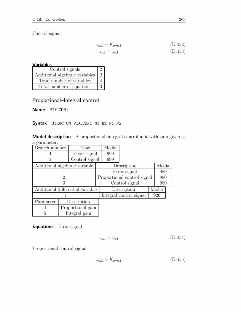
D.18. Controllers 263
Control signal
za,2 = Kpza,1 (D.452)
zc,2 = za,1 (D.453)
VariablesControl signals 2
Additional algebraic variables 2Total number of variables 4Total number of equations 3
Proportional–Integral control
Name PIX CON1
Syntax STRUC CN PIX CON1 N1 N2 P1 P2
Model description A proportional–integral control unit with gain given asa parameter.Branch number Flow Media
1 Error signal 9992 Control signal 999
Additional algebraic variable Description Media1 Error signal 9802 Proportional control signal 9803 Control signal 980
Additional differential variable Description Media1 Integral control signal 920
Parameter Description1 Proportional gain2 Integral gain
Equations Error signal
za,1 = zc,1 (D.454)
Proportional control signal
za,2 = Kpza,1 (D.455)
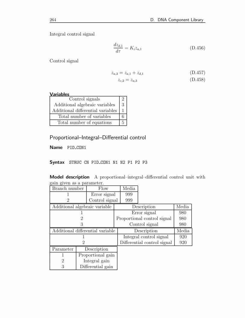
264 D. DNA Component Library
Integral control signal
dzd,1dτ
= Kiza,1 (D.456)
Control signal
za,3 = za,1 + zd,1 (D.457)
zc,2 = za,3 (D.458)
VariablesControl signals 2
Additional algebraic variables 3Additional differential variables 1
Total number of variables 6Total number of equations 5
Proportional–Integral–Differential control
Name PID CON1
Syntax STRUC CN PID CON1 N1 N2 P1 P2 P3
Model description A proportional–integral–differential control unit withgain given as a parameter.Branch number Flow Media
1 Error signal 9992 Control signal 999
Additional algebraic variable Description Media1 Error signal 9802 Proportional control signal 9803 Control signal 980
Additional differential variable Description Media1 Integral control signal 9202 Differential control signal 920
Parameter Description1 Proportional gain2 Integral gain3 Differential gain
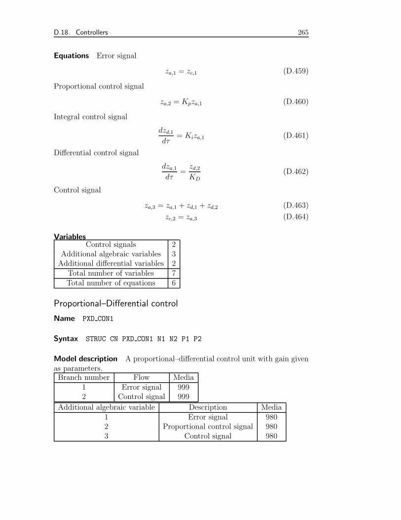
D.18. Controllers 265
Equations Error signal
za,1 = zc,1 (D.459)
Proportional control signal
za,2 = Kpza,1 (D.460)
Integral control signal
dzd,1dτ
= Kiza,1 (D.461)
Differential control signal
dza,1dτ
=zd,2KD
(D.462)
Control signal
za,3 = za,1 + zd,1 + zd,2 (D.463)
zc,2 = za,3 (D.464)
VariablesControl signals 2
Additional algebraic variables 3Additional differential variables 2
Total number of variables 7Total number of equations 6
Proportional–Differential control
Name PXD CON1
Syntax STRUC CN PXD CON1 N1 N2 P1 P2
Model description A proportional–differential control unit with gain givenas parameters.Branch number Flow Media
1 Error signal 9992 Control signal 999
Additional algebraic variable Description Media1 Error signal 9802 Proportional control signal 9803 Control signal 980
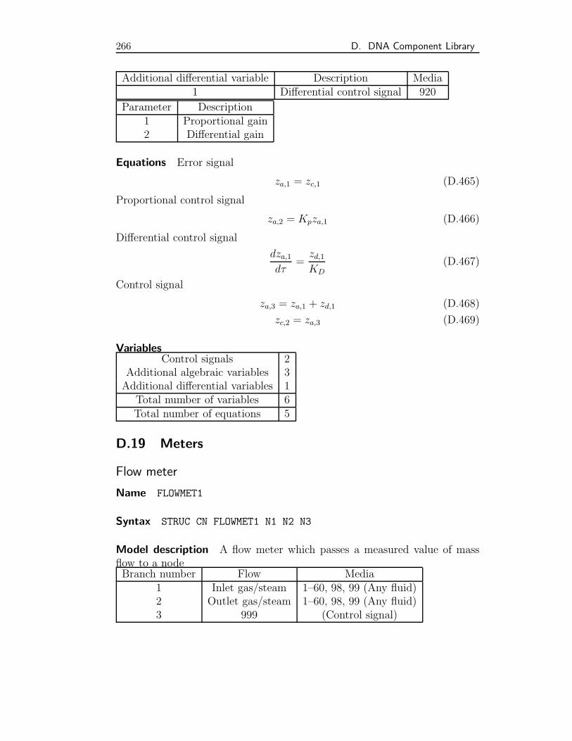
266 D. DNA Component Library
Additional differential variable Description Media1 Differential control signal 920
Parameter Description1 Proportional gain2 Differential gain
Equations Error signal
za,1 = zc,1 (D.465)
Proportional control signal
za,2 = Kpza,1 (D.466)
Differential control signal
dza,1dτ
=zd,1KD
(D.467)
Control signal
za,3 = za,1 + zd,1 (D.468)
zc,2 = za,3 (D.469)
VariablesControl signals 2
Additional algebraic variables 3Additional differential variables 1
Total number of variables 6Total number of equations 5
D.19 Meters
Flow meter
Name FLOWMET1
Syntax STRUC CN FLOWMET1 N1 N2 N3
Model description A flow meter which passes a measured value of massflow to a nodeBranch number Flow Media
1 Inlet gas/steam 1–60, 98, 99 (Any fluid)2 Outlet gas/steam 1–60, 98, 99 (Any fluid)3 999 (Control signal)
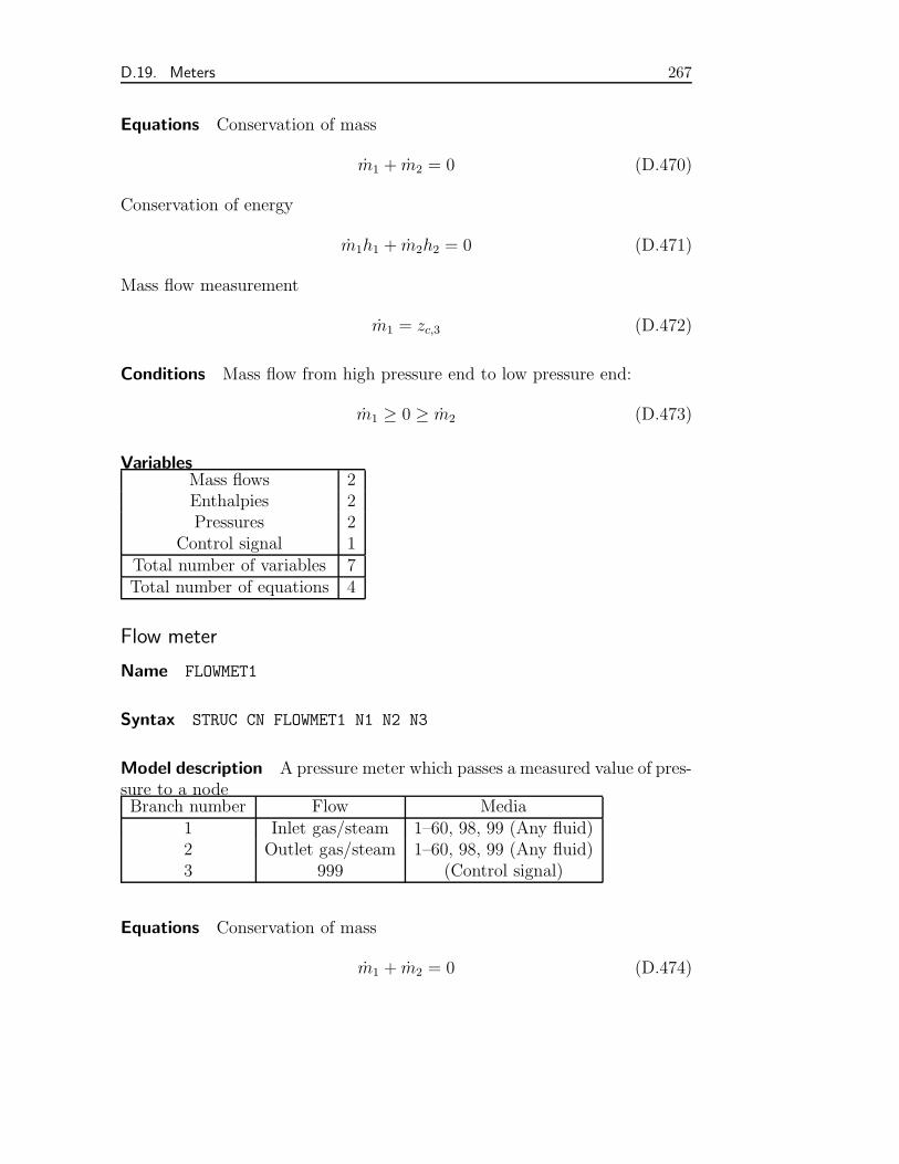
D.19. Meters 267
Equations Conservation of mass
m1 + m2 = 0 (D.470)
Conservation of energy
m1h1 + m2h2 = 0 (D.471)
Mass flow measurement
m1 = zc,3 (D.472)
Conditions Mass flow from high pressure end to low pressure end:
m1 ≥ 0 ≥ m2 (D.473)
VariablesMass flows 2Enthalpies 2Pressures 2
Control signal 1Total number of variables 7Total number of equations 4
Flow meter
Name FLOWMET1
Syntax STRUC CN FLOWMET1 N1 N2 N3
Model description A pressure meter which passes a measured value of pres-sure to a nodeBranch number Flow Media
1 Inlet gas/steam 1–60, 98, 99 (Any fluid)2 Outlet gas/steam 1–60, 98, 99 (Any fluid)3 999 (Control signal)
Equations Conservation of mass
m1 + m2 = 0 (D.474)
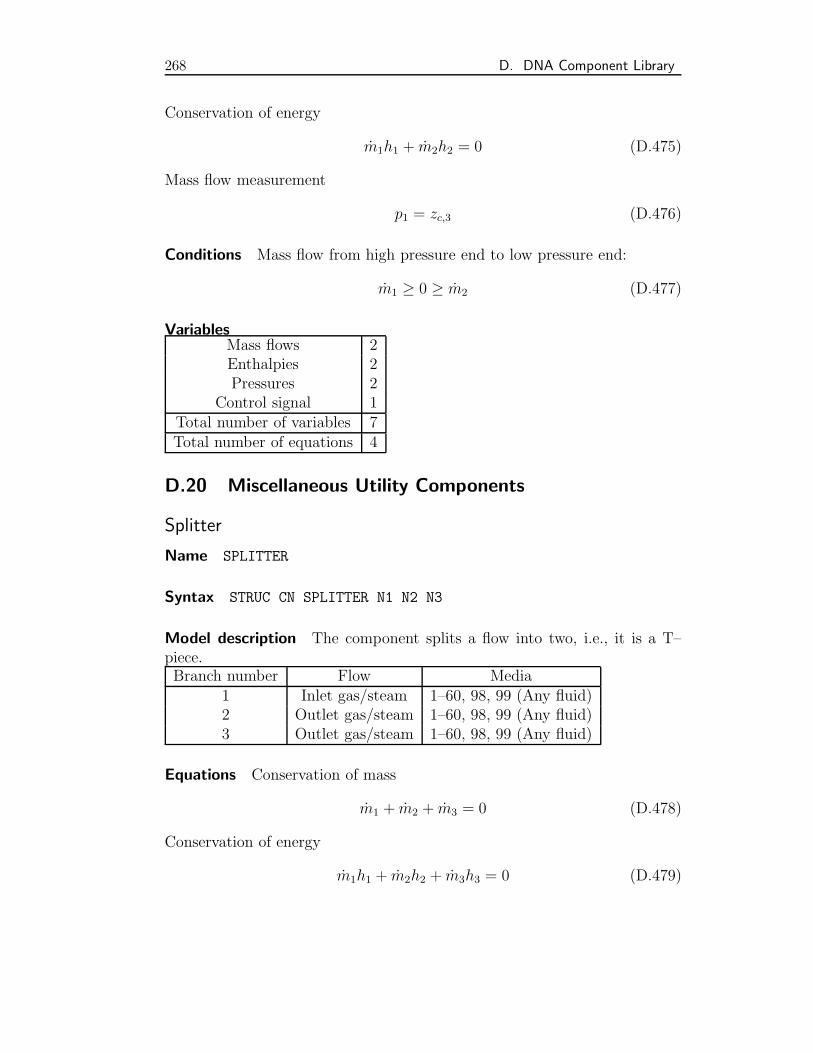
268 D. DNA Component Library
Conservation of energy
m1h1 + m2h2 = 0 (D.475)
Mass flow measurement
p1 = zc,3 (D.476)
Conditions Mass flow from high pressure end to low pressure end:
m1 ≥ 0 ≥ m2 (D.477)
VariablesMass flows 2Enthalpies 2Pressures 2
Control signal 1Total number of variables 7Total number of equations 4
D.20 Miscellaneous Utility Components
Splitter
Name SPLITTER
Syntax STRUC CN SPLITTER N1 N2 N3
Model description The component splits a flow into two, i.e., it is a T–piece.Branch number Flow Media
1 Inlet gas/steam 1–60, 98, 99 (Any fluid)2 Outlet gas/steam 1–60, 98, 99 (Any fluid)3 Outlet gas/steam 1–60, 98, 99 (Any fluid)
Equations Conservation of mass
m1 + m2 + m3 = 0 (D.478)
Conservation of energy
m1h1 + m2h2 + m3h3 = 0 (D.479)
D.20. Miscellaneous Utility Components 269
Enthalpy of outlet flows is the equal
h2 = h3 (D.480)
Pressure is unchanged
p2 = p1 (D.481)
p3 = p1 (D.482)
Conditions Mass flow directions
m1 ≥ 0 (D.483)
m2 ≤ 0 (D.484)
m3 ≤ 0 (D.485)
VariablesMass flows 3Enthalpies 3Pressures 3
Total number of variables 9Total number of equations 5
Usage The component is needed where a flow is split in two because therequirement of equal enthalpy in the outlets is not obtained from the auto-matically applied principles of thermodynamics.
Splitter based on a given ratio
Name FRCSPLIT
Syntax STRUC CN FRCSPLIT N1 N2 N3 P1
Model description The component splits a flow into two, i.e., it is a T–piece. The flow to each outlet is given by a parameterBranch number Flow Media
1 Inlet gas/steam 1–60, 98, 99 (Any fluid)2 Outlet gas/steam 1–60, 98, 99 (Any fluid)3 Outlet gas/steam 1–60, 98, 99 (Any fluid)
270 D. DNA Component Library
Equations Conservation of mass
m1 + m2 + m3 = 0 (D.486)
Conservation of energy
m1h1 + m2h2 + m3h3 = 0 (D.487)
Mass flow to node 2
m2 = rmm1 (D.488)
Enthalpy of outlet flows is the equal
h2 = h3 (D.489)
Pressure is unchanged
p2 = p1 (D.490)
p3 = p1 (D.491)
Conditions Mass flow directions
m1 ≥ 0 (D.492)
m2 ≤ 0 (D.493)
m3 ≤ 0 (D.494)
VariablesMass flows 3Enthalpies 3Pressures 3
Total number of variables 9Total number of equations 5
Splitter for multiple pipes
Name MULSPLIT
Syntax STRUC CN MULSPLIT V1 N1 N2 N3 . . .
D.20. Miscellaneous Utility Components 271
Model description The component splits a flow into more pipes.Branch number Flow Media
1 Inlet gas/steam 1–60, 98, 99 (Any fluid)2 Outlet gas/steam 1–60, 98, 99 (Any fluid)3 Outlet gas/steam 1–60, 98, 99 (Any fluid)
. . .
Equations Conservation of mass∑mi = 0 (D.495)
Conservation of energy ∑mihi = 0 (D.496)
Enthalpy of outlet flows is the equal
h2 = hi, for i = 3, n (D.497)
Pressure is unchanged
pi = p1, for i = 2, n (D.498)
Conditions Mass flow directions
m1 ≥ 0 (D.499)
mi ≤ 0, for i = 2, n (D.500)
VariablesMass flows 3+Enthalpies 3+Pressures 3+
Total number of variables 9+Total number of equations 5+The +’s indicate that the figure is a minimum value.
Usage The component is needed where a flow is split in more than twobecause the requirement of equal enthalpy in the outlets is not obtainedfrom the automatically applied principles of thermodynamics.
Splitter for solid flows
Name SOLSPLIT
272 D. DNA Component Library
Syntax STRUC CN SOLSPLIT N1 N2 N3
Model description The component splits a flow into two, i.e., it is a T–piece.Branch number Flow Media
1 Inlet gas/steam 1–40, 61-80 (Any solid)2 Outlet gas/steam 1–40, 61–80 (Any solid)3 Outlet gas/steam 1–40, 61-80 (Any solid)
Equations Conservation of mass
m1 + m2 + m3 = 0 (D.501)
Conservation of energy
m1h1 + m2h2 + m3h3 = 0 (D.502)
Enthalpy of outlet flows is the equal
h2 = h3 (D.503)
Pressure is unchanged
p2 = p1 (D.504)
p3 = p1 (D.505)
Conditions Mass flow directions
m1 ≥ 0 (D.506)
m2 ≤ 0 (D.507)
m3 ≤ 0 (D.508)
VariablesMass flows 3Enthalpies 3Pressures 3
Total number of variables 9Total number of equations 5
Usage The component is needed where a solid flow is split in two becausethe requirement of equal enthalpy in the outlets is not obtained from theautomatically applied principles of thermodynamics.
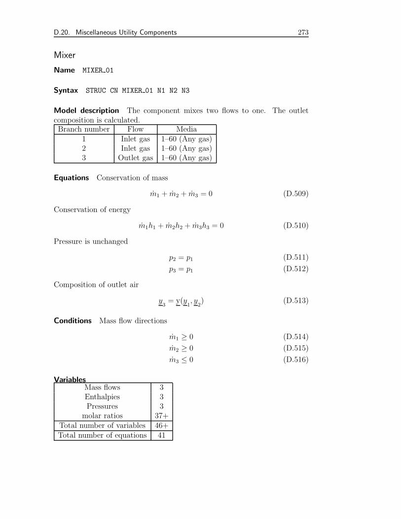
D.20. Miscellaneous Utility Components 273
Mixer
Name MIXER 01
Syntax STRUC CN MIXER 01 N1 N2 N3
Model description The component mixes two flows to one. The outletcomposition is calculated.Branch number Flow Media
1 Inlet gas 1–60 (Any gas)2 Inlet gas 1–60 (Any gas)3 Outlet gas 1–60 (Any gas)
Equations Conservation of mass
m1 + m2 + m3 = 0 (D.509)
Conservation of energy
m1h1 + m2h2 + m3h3 = 0 (D.510)
Pressure is unchanged
p2 = p1 (D.511)
p3 = p1 (D.512)
Composition of outlet air
y3= y(y
1, y
2) (D.513)
Conditions Mass flow directions
m1 ≥ 0 (D.514)
m2 ≥ 0 (D.515)
m3 ≤ 0 (D.516)
VariablesMass flows 3Enthalpies 3Pressures 3
molar ratios 37+Total number of variables 46+Total number of equations 41
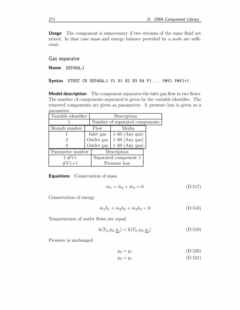
274 D. DNA Component Library
Usage The component is unnecessary if two streams of the same fluid aremixed. In that case mass and energy balance provided by a node are suffi-cient.
Gas separator
Name SEPARA 1
Syntax STRUC CN SEPARA 1 V1 N1 N2 N3 N4 P1 . . . P#V1 P#V1+1
Model description The component separates the inlet gas flow in two flows.The number of components separated is given by the variable identifier. Theremoved components are given as parameters. A pressure loss is given as aparameter.Variable identifier Description
1 Number of separated components
Branch number Flow Media1 Inlet gas 1–60 (Any gas)2 Outlet gas 1–60 (Any gas)3 Outlet gas 1–60 (Any gas)
Parameter number Description1-#V1 Separated component 1#V1+1 Pressure loss
Equations Conservation of mass
m1 + m2 + m3 = 0 (D.517)
Conservation of energy
m1h1 + m2h2 + m3h3 = 0 (D.518)
Temperatures of outlet flows are equal
h(T2, p2, y2) = h(T3, p2, y2
) (D.519)
Pressure is unchanged
p2 = p1 (D.520)
p3 = p1 (D.521)
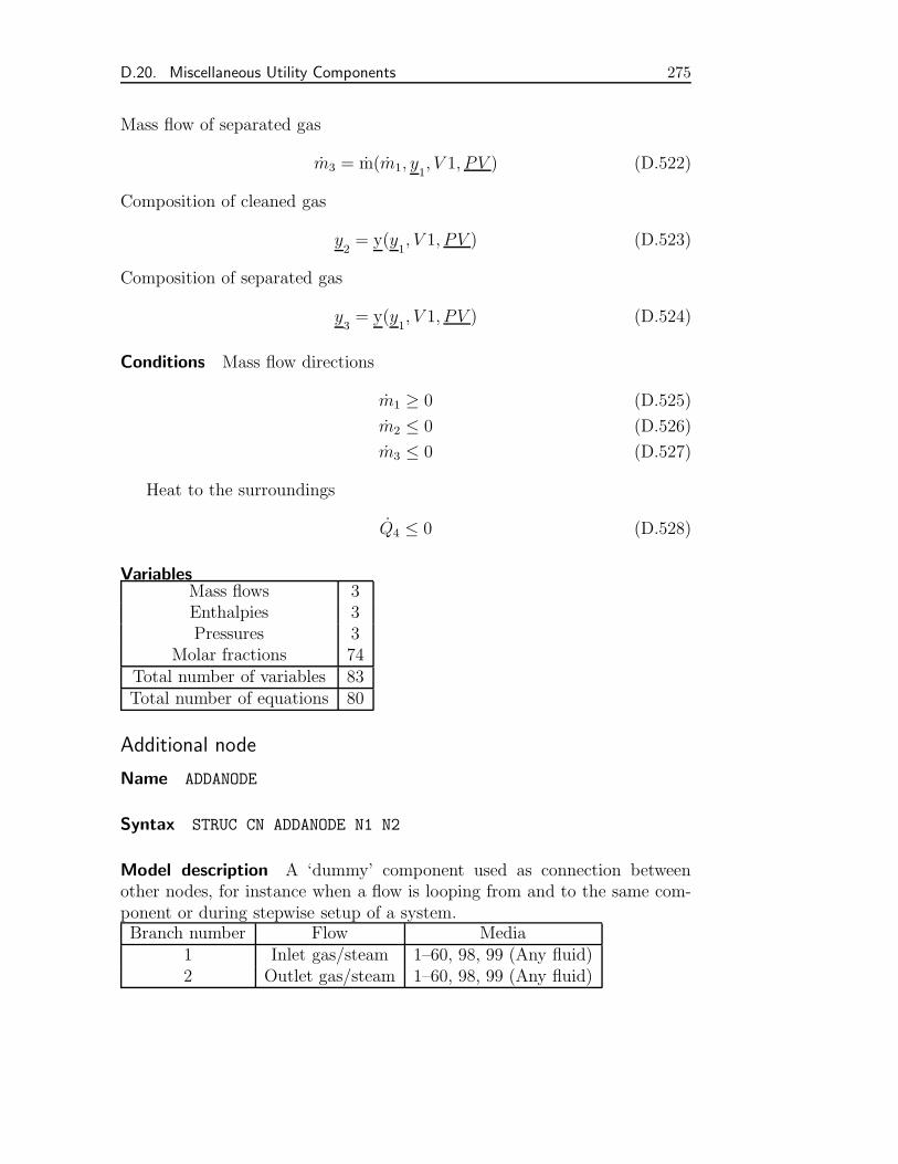
D.20. Miscellaneous Utility Components 275
Mass flow of separated gas
m3 = m(m1, y1, V 1, PV ) (D.522)
Composition of cleaned gas
y2= y(y
1, V 1, PV ) (D.523)
Composition of separated gas
y3= y(y
1, V 1, PV ) (D.524)
Conditions Mass flow directions
m1 ≥ 0 (D.525)
m2 ≤ 0 (D.526)
m3 ≤ 0 (D.527)
Heat to the surroundings
Q4 ≤ 0 (D.528)
VariablesMass flows 3Enthalpies 3Pressures 3
Molar fractions 74Total number of variables 83Total number of equations 80
Additional node
Name ADDANODE
Syntax STRUC CN ADDANODE N1 N2
Model description A ‘dummy’ component used as connection betweenother nodes, for instance when a flow is looping from and to the same com-ponent or during stepwise setup of a system.Branch number Flow Media
1 Inlet gas/steam 1–60, 98, 99 (Any fluid)2 Outlet gas/steam 1–60, 98, 99 (Any fluid)
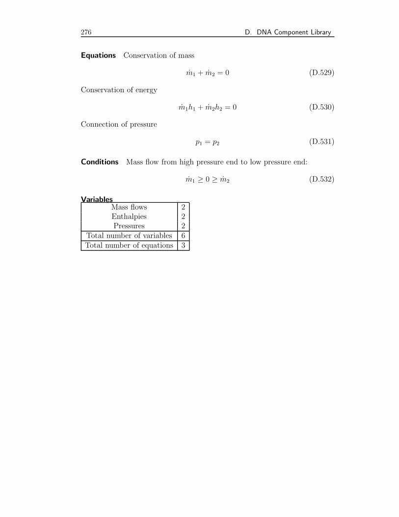
276 D. DNA Component Library
Equations Conservation of mass
m1 + m2 = 0 (D.529)
Conservation of energy
m1h1 + m2h2 = 0 (D.530)
Connection of pressure
p1 = p2 (D.531)
Conditions Mass flow from high pressure end to low pressure end:
m1 ≥ 0 ≥ m2 (D.532)
VariablesMass flows 2Enthalpies 2Pressures 2
Total number of variables 6Total number of equations 3
E. DNA INPUT
Input file with Generated Guesses
The following input files show the difference in the size of files with andwithout initial guesses supplied by the user. The files show the input to amodel of an IGCC installation. The model has been formulated by Lorentzen[72] and is part of the DNA samples distributed with the code. It should benoticed that also component types have been changed. This is due to thegeneralization of the interface of the DNA component library.
Old DNA Input
The first file is the file written by Lorentzen:
STRUC 1 GTW_HEX1 24 25 10 11 0 0STRUC 2 WAT_EVA2 23 24 11 12 10 0 0STRUC 3 GTW_HEX1 22 23 12 13 0 0STRUC 4 STE_TUR1 13 14 31 0.82STRUC 5 SIM_GENE 42 43 31 0.98STRUC 6 WTW_HEX1 14 15 16 17 0 0STRUC 7 WAT_PUM1 15 10 44 0.92
STRUC 9 GAS_BUR1 19 20 21 45 56 1STRUC 8 AIR_COM1 18 19 30 0.79 16STRUC 10 GAS_TUR1 21 22 30 0.89STRUC 11 SIM_GENE 40 41 30 0.98
START P 18 1 P 19 16 P 20 16 P 21 16 P 22 1.5 P 23 1.5 P 24 1.5 P 25 1.5START M 8 18 250 M 8 19 -250 M 9 19 250 M 9 20 4 M 9 21 -254START M 10 21 254 M 10 22 -254 M 3 23 -254 M 2 23 254START M 2 24 -254 M 1 24 254 M 1 25 -254 M 3 22 254START T 8 18 24 T 8 19 250 T 9 19 250 T 9 20 25 T 9 21 1000START T 10 21 1000 T 10 22 700 T 3 22 700 T 3 23 500 T 2 23 500START T 2 24 300 T 1 24 300 T 1 25 100START E 11 40 -70000 Q 11 41 -1400 Q 9 45 0
278 E. DNA Input
ADDCO M 8 18 300 T 8 18 24 P 18 1.01 T 9 20 25 Q 9 45 0ADDCO T 10 22 650
START P 10 50 P 11 50 P 12 50 P 13 50 P 14 0.2 P 15 0.2START P 16 1 P 17 1
START E 5 42 -70000 Q 5 43 -1400 E 7 44 300
START M 1 10 80 M 1 11 -80 M 2 11 80 M 2 12 -80 M 3 12 80START M 3 13 -80 M 4 13 80 M 4 14 -80 M 6 14 80 M 6 15 -80START M 6 16 4000 M 6 17 -4000 M 7 15 80 M 7 10 -80
START H 1 10 300 H 1 11 1200 H 2 11 1200 H 2 12 2800 H 3 12 2800START H 3 13 3100 H 4 13 3100 H 4 14 2600 H 6 14 2600 H 6 15 300START H 6 16 42 H 6 17 75 H 7 15 300 H 7 10 301
ADDCO X 6 15 0 P 15 0.2 P 10 50 P 16 1 X 2 12 1ADDCO T 3 13 500 T 6 17 20 T 6 16 10 T 1 11 250
The number of initial guesses equals the number of variables in the systemand is 76. It is obvious that trivial initializations as equalizing the input andoutput in a component or a node and as applying condition values as initialguesses are annoying.
New DNA Input
The new input file not only exploits the reduced number of guesses but alsoshows an improved structuring of the model and the use of comments in thefile.
TITLE COMBINED CYCLE
C EconomizerSTRUC 1 HEATEX_1 24 25 10 11 301 0 0ADDCO T 2 11 250 Q 1 301 0
C EvaporatorSTRUC 2 WAT_EVA2 23 24 11 12 10 0 0ADDCO X 2 12 1
C SuperheaterSTRUC 3 HEATEX_1 22 23 12 13 303 0 0ADDCO T 3 13 500 Q 3 303 0
279
C TurbineSTRUC 4 TURBIN_1 13 14 105 0.82ADDCO P 13 50START T 4 13 500
C GeneratorSTRUC 5 SIM_GENE 205 305 105 0.98START Q 5 305 -10
C CondenserSTRUC 6 STECON_1 14 15 16 17 0 0MEDIA 14 99 16 99ADDCO P 15 0.2 P 16 1 T 6 16 10 T 6 17 20START M 6 16 1000 X 6 15 0
C Feed water pumpSTRUC 7 WAT_PUM1 15 10 207 0.92START E 7 207 10START M 6 14 55.4
C Gas combustorSTRUC 9 GASBUR_1 19 20 21 45 56 1MEDIA 19 9 20 3 21 30ADDCO T 9 20 25 Q 9 45 0START M 9 20 5
C CompressorSTRUC 8 COMPRE_1 18 19 308 111 0.79 1ADDCO M 8 18 300 T 8 18 24 P 18 1.01 P 19 16START T 8 19 500 Q 8 308 0
C Gas turbineSTRUC 10 TURBIN_1 21 22 111 0.89ADDCO T 10 22 650START P 22 1.5
C GeneratorSTRUC 11 SIM_GENE 211 311 111 0.98START Q 11 311 -10
The number of initial guesses has been reduced to 11 (=14%). This reductionof guesses will increase with the size of the system. The number of neededinitial guesses will be in the range of the number of constitutive relations inthe model.

280 E. DNA Input
F. FUTURE DEVELOPMENT OF DNA
Throughout this thesis DNA has been claimed to have unique features andto be a very promising tool for engineers working with energy system studiesin virtually any field. However, the program has only been applied in a fewstudies compared to notable commercial codes. Furthermore, most of thesestudies have focussed on system layout applying highly simplified models forthe devices. To see if the program is as good as claimed I highly recommendthat future studies approach modelling and improvement of existing or futureindustrial installations. In order to do this, it will be necessary to have ahigher level of cooperation with industry.
Graphical User Interface
Modern computer programs allow users to work in a graphical environment.This has also by Lorentzen[72] been regarded as an important improvementof DNA. In order to allow new users to get acquainted with the programmuch easier a graphical user interface need to be developed. However, in myopinion it is important to develop a graphical interface with respect to thePREFUR framework. The main issues to focus on in the case of a graphicalenvironment is:
Portability The interface has to be the same for any operating system.There seems to be two ways to obtain this:
Either the basic graphical elements, such as lines, circles and so onshould be implemented in system-dependent code. This may requiredifferent implementations for different compilers on the same system,but allows access to all parts of the code.
Otherwise, one may use a scripting language, such as tcl/tk1, whichhas a library for implementation of graphical interface in virtually anyoperating system and thereby is portable. tcl/tk is a freeware program,so any user may obtain it. The problem with this approach is that theimplementation has to rely on foreign developments.
1 A thorough description of the tcl/tk language is found in E. F. Johnson: ‘GraphicalApplications with Tcl and TK’, MT Books, 1996
282 F. Future Development of DNA
Flexibility The interface should give the user access to any functionalityof DNA. This requires new developments of DNA to be implementedin the interface also. Another issue with respect to flexibility is thatexperienced users may like to work with the text-based DNA file, be-cause it may be much faster and precision of, for instance positioningof components in the graphical interface, may be enhanced. This func-tionality should be possible so the program may work both ways. Inputto the graphical interface should be reflected in the text input file andvice versa.
Robustness and User-friendliness are of course of high importance.
Equation Parser
Users of the program have to compile the code, and thereby need access toand knowledge of a FORTRAN compiler. These are available as freeware,but some users may like to avoid this step. If, on the other hand, the programis distributed as a compiled executable, users cannot access and extend thecomponent library. One way to overcome this problem is to include a routine,which can read a text-based input representing a component model. Themain problem to handle in this development is to include a compiler orparser, which reads the mathematical relations in a component.
Component Library
The component library has been highly simplified, by the extended featuresof DNA, implemented during this study. One suggestion which might be con-sidered to improve the structure of the library is to include a set of identifiers,which might be accessed from a component. When used, these might specifywhich one of a number of universal models available for a given character-istic, to use. An example: Pressure loss in a pipe is modelled by applyingeither a zero, a constant value, a mass-dependent value, an inlet-pressure-dependent value, a friction factor or another specific approach. A model ofa heat exchanger with two flows applying a specified model for heat trans-fer may be used in conjunction with each of the pressure loss models. Thismeans that any heat transfer model may be used with, say 62 = 36, pressureloss models in theory. To complete the component library and allow all thesepossibilities together with say about five heat transfer models would blowup the component library. Instead by specifying each pressure loss model,heat transfer model and so on in a separate routine with a specified interface
283
called from the component routines according to identifiers would overcomethis problem and improve the readability of the program.
Programming the Code
As is DNA is written in almost without exception pure ANSI standard FOR-TRAN77. The main exceptions are use of command line parsing, ENDDOstatements, INCLUDE directives and special characters, like underscore, invariable names. Only reading of the command line is not included in thenewer FORTRAN90 standard [30], of which FORTRAN77 is a fixed-formsubset. Translation of DNA to free-form FORTRAN90 would not only allowa neater looking code to be written by inclusion of CASE constructs insteadof IF--THEN--ELSEIF--ENDIF which are used a lot. Also, the use of pointersand thereby dynamic memory allocation may be applied. DNA is workingwith pointers in three globally used one-dimensional arrays. These arrays areupdated in an ingenious way, which is not simple to understand and workwith [72]. Also these arrays have to be ‘large enough’, which means thattheir size is predefined in the ENVIRO.INI file. To have large enough globalarrays these become much larger than in fact needed during simulation, be-cause the sizes of the arrays used during setup of the system structure isunknown and therefore have to be assumed to have the maximum allowedsize. After the system is set up, the arrays are shortened, but the globalarrays and thereby the executable DNA program have the same size. Fur-thermore, FORTRAN90 allows the use of variables with a predefined input oroutput nature, so variables in global routines may be protected from changesmade by component routines.
Controlling the Numerical Solution
It has been found that the robustness of the model may be improved byintroduction of generally valid equations. The solver, however, still has to becontrolled carefully, when a ‘weak’ branch of an equation is entered. A wayto make the program control the increase in the residuals or displacementsbefore updating the Jacobian and to control the damping of an iteration stepin the Newton method would be interesting to include in the program.
One issue to focus on is the differences between solving a steady-statemodel and a dynamic model. In the dynamic model, the initial time stepis similar to a steady-state model, whereas the remaining time steps aredifferent. The numerical parameters controlling the solution are the samethroughout the whole simulation, however, and a control of these may be of
284 F. Future Development of DNA
interest to study, in order to make DNA more robust.
Dynamic Shafts
The possibility of simulating turbine shafts at transient conditions in DNA,has not been applied in simulations. It is of interest to try to use this featurein the future.
Three-flow components
As is DNA does not allow components to have more than two separate flows.Some parts of a power plant cannot be modelled because of this assumption,because three flows are present. Therefore an extension of the program tohandle more general components seems interesting.
Refrigerants and Material Properties
DNA is claimed to be applicable to any energy system model. One classof systems, refrigeration installations, are not possible to model, because thethermo-physical properties of refrigerants are not available. These are neededfor further studies.
In this study DNA has been applied in off-design load studies. Thishas required implementation of more comprehensive models including thethermal properties of the construction material of the plant equipment. The(temperature-dependent) properties of common materials might be madegenerally available in the code.
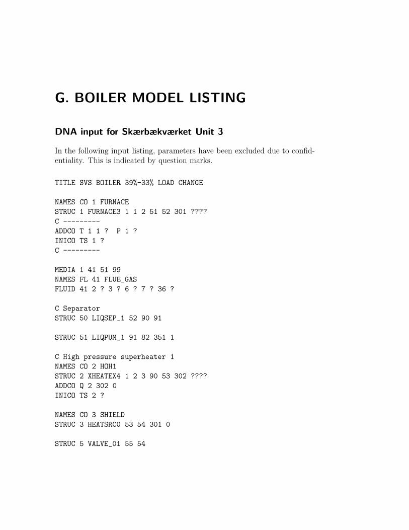
G. BOILER MODEL LISTING
DNA input for Skærbækværket Unit 3
In the following input listing, parameters have been excluded due to confid-entiality. This is indicated by question marks.
TITLE SVS BOILER 39%-33% LOAD CHANGE
NAMES CO 1 FURNACE
STRUC 1 FURNACE3 1 1 2 51 52 301 ????
C ---------
ADDCO T 1 1 ? P 1 ?
INICO TS 1 ?
C ---------
MEDIA 1 41 51 99
NAMES FL 41 FLUE_GAS
FLUID 41 2 ? 3 ? 6 ? 7 ? 36 ?
C Separator
STRUC 50 LIQSEP_1 52 90 91
STRUC 51 LIQPUM_1 91 82 351 1
C High pressure superheater 1
NAMES CO 2 HOH1
STRUC 2 XHEATEX4 1 2 3 90 53 302 ????
ADDCO Q 2 302 0
INICO TS 2 ?
NAMES CO 3 SHIELD
STRUC 3 HEATSRC0 53 54 301 0
STRUC 5 VALVE_01 55 54
286 G. Boiler Model Listing
ADDCO T 4 56 ?
C High pressure superheater 2
NAMES CO 4 HOH2
STRUC 4 XHEATEX4 2 3 4 54 56 304 ????
ADDCO Q 4 304 0
INICO TS 4 ?
C Splitting gas flow for reheaters
STRUC 6 FRCSPLIT 4 5 6 .5
C Pressure measurement
STRUC 7 PRESSO_1 56 57 907
C High pressure turbine
STRUC 8 TURBIN_2 57 58 130 ???
C Extraction
STRUC 9 EXTRACT1 58 59 60 907 ???
C Intermediate pressure reheater 1.2
NAMES CO 10 MOH1.2
STRUC 10 XHEATEX4 2 5 7 66 67 310 ????
ADDCO Q 10 310 0
INICO TS 10 ?
STRUC 11 TURBIN_2 67 68 130 ?
STRUC 12 EXTRACT1 68 69 70 907 ?
C Deconnecting gas presures from MOH1.2 and MOH 2.2
STRUC 13 VALVE_01 8 7
C Intermediate pressure reheater 2.2
NAMES CO 14 MOH2.2
STRUC 14 XHEATEX4 2 6 8 71 73 314 ????
ADDCO Q 14 314 0
INICO TS 14 ?
STRUC 15 TURBIN_2 73 74 130 ??
ADDCO P 74 ?
287
C Intermediate pressure reheater 1.1B
NAMES CO 16 MOH1.1B
STRUC 16 XHEATEX4 3 7 9 64 66 316 ????
ADDCO Q 16 316 0
INICO TS 16 ?
STRUC 17 VALVE_01 65 66
ADDCO T 10 67 ?
C Intermediate pressure reheater 2.1
NAMES CO 18 MOH2.1
STRUC 18 XHEATEX4 3 9 10 70 71 318 ????
ADDCO Q 18 318 0
INICO TS 18 ?
STRUC 19 VALVE_01 72 71
ADDCO T 14 73 ?
C Intermediate pressure reheater 1.1A
NAMES CO 20 MOH1.1A
STRUC 20 XHEATEX5 4 10 11 60 64 320 ????
ADDCO Q 20 320 0
INICO TS 20 ?
C Economiser
NAMES CO 21 ECO
STRUC 21 XHEATEX5 6 11 12 88 82 321 ????
MEDIA 88 99
ADDCO T 21 88 ?
ADDCO Q 21 321 0
INICO TS 21 ?
NAMES CO 22 DOWNCOMER
STRUC 22 DOWNCOM1 82 51 70 ?
STRUC 23 STECON_0 74 75 340 0
C START X 23 75 0
STRUC 24 LIQPUM_1 75 76 224 1
288 G. Boiler Model Listing
STRUC 25 STECON_1 69 77 76 78 0 0
STRUC 26 LIQPUM_1 77 78 326 1
STRUC 27 STECON_1 59 79 78 80 0 0
STRUC 28 LIQPUM_1 79 80 328 1
STRUC 29 HEATSRC0 89 81 329 0
STRUC 41 PRESCON1 81 88 940 ??
STRUC 42 CON_VAL3 3 100 101 ????
STRUC 30 SIM_GENE 230 330 130 1
STRUC 99 MULSPLIT 4 80 89 72 65 55
STRUC 40 FLOWMET1 101 1 940
UPDAT
Initial guesses are in an include file due to the UPDAT key word.
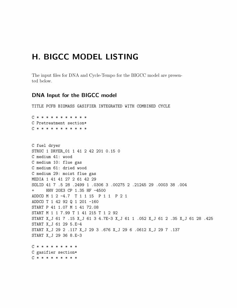
H. BIGCC MODEL LISTING
The input files for DNA and Cycle-Tempo for the BIGCC model are presen-ted below.
DNA Input for the BIGCC model
TITLE PCFB BIOMASS GASIFIER INTEGRATED WITH COMBINED CYCLE
C * * * * * * * * * * *
C Pretreatment section*
C * * * * * * * * * * *
C fuel dryer
STRUC 1 DRYER_01 1 41 2 42 201 0.15 0
C medium 41: wood
C medium 10: flue gas
C medium 61: dried wood
C medium 29: moist flue gas
MEDIA 1 41 41 27 2 61 42 29
SOLID 41 7 .5 28 .2499 1 .0306 3 .00275 2 .21245 29 .0003 38 .004
+ HHV 20E3 CP 1.35 HF -4500
ADDCO M 1 2 -4.7 T 1 1 15 P 1 1 P 2 1
ADDCO T 1 42 92 Q 1 201 -160
START P 41 1.07 M 1 41 72.08
START M 1 1 7.99 T 1 41 215 T 1 2 92
START X_J 61 7 .15 X_J 61 3 4.7E-3 X_J 61 1 .052 X_J 61 2 .35 X_J 61 28 .425
START X_J 61 29 5.E-4
START X_J 29 2 .117 X_J 29 3 .676 X_J 29 6 .0612 X_J 29 7 .137
START X_J 29 36 8.E-3
C * * * * * * * * *
C gasifier section*
C * * * * * * * * *
290 H. BIGCC Model Listing
C Splitting fuel for two gasifiers
STRUC 2 SOLSPLIT 2 3 4
START T 2 4 92
C High equilibirum temperature/high AF gasifier
STRUC 3 GASIFI_0 3 90 33 5 6 303 25 785 1 0 .985
MEDIA 33 9 5 21 6 69
C Medium 9: Air
C Medium 21: Syngas 1
C Medium 69: Ashes
ADDCO T 3 90 70 M 3 3 3.8 Q 3 303 -480 P 6 1
START P 90 26 P 33 26 P 5 25.0
START M 3 90 0.00E0 M 3 6 -5.0E-2 T 3 6 796 T 3 5 796 M 3 33 4.2
START X_J 21 1 0.1718 X_J 21 3 0.3425 X_J 21 4 0.2080 X_J 21 6 0.1207
START X_J 21 7 0.0873
START X_J 21 8 4.2E-4 X_J 21 9 1.8E-4 X_J 21 11 0.0650 X_J 21 36 4.1E-3
START X_J 69 38 0.516 X_J 69 28 .483
START ZA 3 1 0
C Low equilibirum temperature/low AF gasifier
STRUC 4 GASIFI_0 4 91 34 7 8 304 25 390 1 0 .97
MEDIA 34 9 7 22 8 70
C Medium 9: Air
C Medium 22: Syngas 2
C Medium 70: Ashes
ADDCO T 4 91 70 M 4 34 3.6 Q 4 304 -380 P 8 1
START P 91 26 P 34 26 P 7 25.0 Q 4 304 -4.E2
START M 4 91 0.00E0 M 4 8 -1.7E-2 T 4 8 1.88E3 T 4 7 1892
START X_J 22 1 6.5E-3 X_J 22 3 0.6240 X_J 22 4 5.4E-4 X_J 22 6 0.1802
START X_J 22 7 0.1617
START X_J 22 8 1.6E-4 X_J 22 9 9.2E-5 X_J 22 11 0.01893 X_J 22 36 7.4E-3
START X_J 70 38 0.347 X_J 70 28 .652
START ZA 4 1 0
STRUC 5 VALVE_01 7 9
C Syngas mixer
STRUC 6 MIXER_01 5 9 10
MEDIA 10 23
C Medium 23: Produced syngas
291
START X_J 23 1 0.1197 X_J 23 3 0.430 X_J 23 4 0.1426
START X_J 23 6 0.1395
START X_J 23 7 0.1107
START X_J 23 8 3.4E-4 X_J 23 9 1.4E-4 X_J 23 11 0.0504 X_J 23 36 5.1E-3
C Gas cleaner
STRUC 8 GASCLE_1 11 12 13 308 0
MEDIA 12 24 13 25
C Medium 24: Cleaned syngas
C Medium 25: Removed gas
ADDCO Q 8 308 0
START M 8 13 -5.E-3 T 8 13 499
START X_J 24 1 0.1199 X_J 24 3 0.4314 X_J 24 4 0.1427
START X_J 24 6 0.1395
START X_J 24 7 0.1107
START X_J 24 11 0.05049 X_J 24 36 5.1E-3
START X_J 25 8 .68 X_J 25 9 .31
C * * * * * * * * * * *
C Gas turbine section
C * * * * * * * * * * *
C air compressor
STRUC 21 COMPRE_1 20 21 321 133 0.8313 .997
MEDIA 20 9
C Medium 9: Air
ADDCO M 21 20 68 T 21 20 15 P 20 1.013
ADDCO P 21 19.4
START T 21 21 457 Q 21 321 -94.19
C cooling air
STRUC 22 SPLITTER 21 22 26
ADDCO M 22 26 -9.5
START T 22 22 457
C Air loss
STRUC 28 SPLITTER 22 23 25
ADDCO M 28 25 -.544
START T 28 23 457
C gasification air
292 H. BIGCC Model Listing
STRUC 23 SPLITTER 23 24 27
START M 23 27 -7.87
START T 23 24 457
C gas combustor
STRUC 24 GASBUR_2 24 12 35 324 1168 .97
MEDIA 35 26
C Medium 26: Combustion products
ADDCO Q 24 324 -217
VARPA 24 1 M 23 27 -7.88
START M 24 24 50 T 24 35 1168 P 35 18.8
START X_J 26 2 .1137 X_J 26 3 .7184 X_J 26 6 .0758 X_J 26 7 .0833
START X_J 26 36 8.5E-3
C Cooling air mixer
STRUC 25 MIXER_01 35 36 37
MEDIA 37 27
C Medium 27: Turbine inlet gas
START X_J 27 2 .1262 X_J 27 3 .7256 X_J 27 6 .0657 X_J 27 7 .0737
START X_J 27 36 8.5E-3
STRUC 26 VALVE_01 26 36
MEDIA 36 9
C Gas turbine
STRUC 27 TURBIN_1 37 38 133 .8953
ADDCO P 38 1.07
START T 27 38 483
STRUC 33 SIM_GENE 233 333 133 0.98
START E 33 233 -20688
C Booster compressor
STRUC 29 COMPRE_1 28 29 329 129 .7856 .9
ADDCO P 29 26
START T 29 29 96 Q 29 329 -32.67
STRUC 30 SPLITTER 30 31 32
START T 30 31 90
STRUC 31 VALVE_01 31 33
293
STRUC 32 VALVE_01 32 34
C * * * * * * *
C Steam cycle *
C * * * * * * *
C Economiser
STRUC 40 HEATEX_1 40 41 60 61 340 0 3
ADDCO T 40 61 257.84 Q 40 340 0
C Steam drum
STRUC 41 STEDRU_0 61 67 166 62 341 67
ADDCO Q 41 341 -150
STRUC 42 SPLITTER 62 63 65
C Flue gas cooling evaporator
STRUC 43 HEATEX_1 39 40 63 64 343 0 0
START T 43 40 288
ADDCO X 43 64 0.5 Q 43 343 0
START M 43 63 1.E1
C Syngas cooling evaporator
STRUC 44 HEATEX_1 10 11 65 66 344 0 0
ADDCO T 44 11 500 Q 44 344 -225
ADDCO X 44 66 0.5
START M 44 65 16.2 P 65 67 H 44 65 1.E3
C Flue gas cooling superheater
STRUC 45 HEATEX_1 38 39 67 68 345 0 6.7
START T 45 39 403
ADDCO T 45 68 443 Q 45 345 0
C Extraction turbine
STRUC 46 TURCYCLE 4 68 78 77 69 146 .77
ADDCO P 78 8 P 77 2
START H 46 77 2750 H 46 78 2948 H 46 69 2285 M 46 77 -5.E-1 M 46 78 -.95
STRUC 57 SIM_GENE 246 346 146 0.98
START E 57 246 -11833
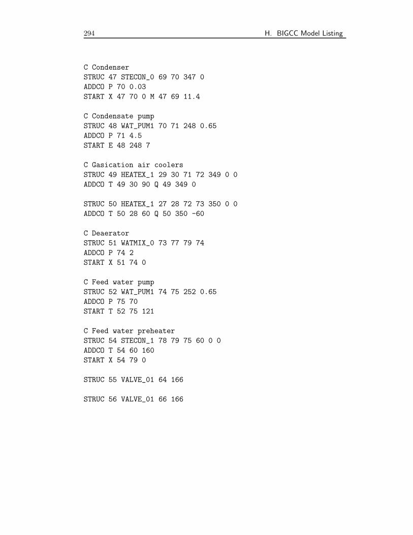
294 H. BIGCC Model Listing
C Condenser
STRUC 47 STECON_0 69 70 347 0
ADDCO P 70 0.03
START X 47 70 0 M 47 69 11.4
C Condensate pump
STRUC 48 WAT_PUM1 70 71 248 0.65
ADDCO P 71 4.5
START E 48 248 7
C Gasication air coolers
STRUC 49 HEATEX_1 29 30 71 72 349 0 0
ADDCO T 49 30 90 Q 49 349 0
STRUC 50 HEATEX_1 27 28 72 73 350 0 0
ADDCO T 50 28 60 Q 50 350 -60
C Deaerator
STRUC 51 WATMIX_0 73 77 79 74
ADDCO P 74 2
START X 51 74 0
C Feed water pump
STRUC 52 WAT_PUM1 74 75 252 0.65
ADDCO P 75 70
START T 52 75 121
C Feed water preheater
STRUC 54 STECON_1 78 79 75 60 0 0
ADDCO T 54 60 160
START X 54 79 0
STRUC 55 VALVE_01 64 166
STRUC 56 VALVE_01 66 166
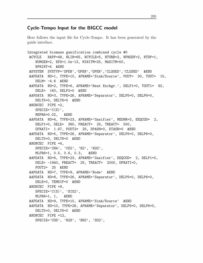
295
Cycle-Tempo Input for the BIGCC model
Here follows the input file for Cycle-Tempo. It has been generated by theguide interface.
Integrated biomass gasification combined cycle #0
&CYCLE NAPP=48, NLIN=65, NCYCLE=5, NTURB=2, NPRODF=2, NTDP=1,
NUMGEN=2, EPS=1.0e-13, MINITM=25, MAXITM=50,
NPRINT=4 &END
&SYSTEM SYSTYP=’OPEN’,’OPEN’,’OPEN’,’CLOSED’,’CLOSED’ &END
&APDATA NO=1, TYPE=10, APNAME=’Sink/Source’, POUT= 30, TOUT= 15,
DELM= -4.6 &END
&APDATA NO=2, TYPE=6, APNAME=’Heat Exchgr.’, DELP1=0, TOUT1= 92,
DELE= 160, DELP2=0 &END
&APDATA NO=3, TYPE=26, APNAME=’Separator’, DELP5=0, DELP6=0,
DELT5=0, DELT6=0 &END
&NONCEC PIPE =2,
SPECIE=’C(S)’,
MSFR6=0.02, &END
&APDATA NO=4, TYPE=23, APNAME=’Gasifier’, MEDNR=3, EEQCOD= 2,
DELP1=0, DELE= 380, PREACT= 25, TREACT= 500,
OFRATI= 1.67, POUT2= 25, DPASH=0, DTASH=0 &END
&APDATA NO=5, TYPE=26, APNAME=’Separator’, DELP5=0, DELP6=0,
DELT5=0, DELT6=0 &END
&NONCEC PIPE =4,
SPECIE=’CH4’, ’CO2’, ’H2’, ’H2O’,
MLFR6=1, 0.5, 0.6, 0.3, &END
&APDATA NO=6, TYPE=23, APNAME=’Gasifier’, EEQCOD= 2, DELP1=0,
DELE= -1940, PREACT= 25, TREACT= 2000, OFRATI=0,
POUT2= 25 &END
&APDATA NO=7, TYPE=9, APNAME=’Node’ &END
&APDATA NO=8, TYPE=26, APNAME=’Separator’, DELP5=0, DELP6=0,
DELE=0, TEMDIF=0 &END
&NONCEC PIPE =9,
SPECIE=’C(S)’, ’SIO2’,
MLFR6=1, 1, &END
&APDATA NO=9, TYPE=10, APNAME=’Sink/Source’ &END
&APDATA NO=10, TYPE=26, APNAME=’Separator’, DELP5=0, DELP6=0,
DELT5=0, DELT6=0 &END
&NONCEC PIPE =12,
SPECIE=’COS’, ’H2S’, ’NH3’, ’SO2’,
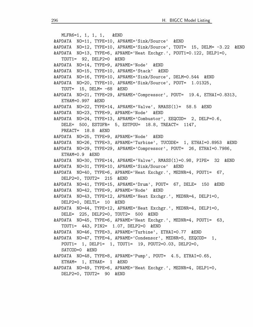
296 H. BIGCC Model Listing
MLFR6=1, 1, 1, 1, &END
&APDATA NO=11, TYPE=10, APNAME=’Sink/Source’ &END
&APDATA NO=12, TYPE=10, APNAME=’Sink/Source’, TOUT= 15, DELM= -3.22 &END
&APDATA NO=13, TYPE=6, APNAME=’Heat Exchgr.’, POUT1=0.122, DELP1=0,
TOUT1= 92, DELP2=0 &END
&APDATA NO=14, TYPE=9, APNAME=’Node’ &END
&APDATA NO=15, TYPE=10, APNAME=’Stack’ &END
&APDATA NO=16, TYPE=10, APNAME=’Sink/Source’, DELM=0.544 &END
&APDATA NO=20, TYPE=10, APNAME=’Sink/Source’, POUT= 1.01325,
TOUT= 15, DELM= -68 &END
&APDATA NO=21, TYPE=29, APNAME=’Compressor’, POUT= 19.4, ETHAI=0.8313,
ETHAM=0.997 &END
&APDATA NO=22, TYPE=14, APNAME=’Valve’, RMASS(1)= 58.5 &END
&APDATA NO=23, TYPE=9, APNAME=’Node’ &END
&APDATA NO=24, TYPE=13, APNAME=’Combustor’, EEQCOD= 2, DELP=0.6,
DELE= 500, ESTOFR= 5, ESTPOU= 18.8, TREACT= 1147,
PREACT= 18.8 &END
&APDATA NO=25, TYPE=9, APNAME=’Node’ &END
&APDATA NO=26, TYPE=3, APNAME=’Turbine’, TUCODE= 1, ETHAI=0.8953 &END
&APDATA NO=29, TYPE=29, APNAME=’Compressor’, POUT= 26, ETHAI=0.7986,
ETHAM=0.9 &END
&APDATA NO=30, TYPE=14, APNAME=’Valve’, RMASS(1)=0.98, PIPE= 32 &END
&APDATA NO=31, TYPE=10, APNAME=’Sink/Source’ &END
&APDATA NO=40, TYPE=6, APNAME=’Heat Exchgr.’, MEDNR=4, POUT1= 67,
DELP2=0, TOUT2= 215 &END
&APDATA NO=41, TYPE=15, APNAME=’Drum’, POUT= 67, DELE= 150 &END
&APDATA NO=42, TYPE=9, APNAME=’Node’ &END
&APDATA NO=43, TYPE=12, APNAME=’Heat Exchgr.’, MEDNR=4, DELP1=0,
DELP2=0, DELTL= 10 &END
&APDATA NO=44, TYPE=12, APNAME=’Heat Exchgr.’, MEDNR=4, DELP1=0,
DELE= 225, DELP2=0, TOUT2= 500 &END
&APDATA NO=45, TYPE=6, APNAME=’Heat Exchgr.’, MEDNR=4, POUT1= 63,
TOUT1= 443, PIN2= 1.07, DELP2=0 &END
&APDATA NO=46, TYPE=3, APNAME=’Turbine’, ETHAI=0.77 &END
&APDATA NO=47, TYPE=4, APNAME=’Condensor’, MEDNR=5, EEQCOD= 1,
POUT1= 1, DELP1= 1, TOUT1= 19, POUT2=0.03, DELP2=0,
SATCOD=0 &END
&APDATA NO=48, TYPE=8, APNAME=’Pump’, POUT= 4.5, ETHAI=0.65,
ETHAM= 1, ETHAE= 1 &END
&APDATA NO=49, TYPE=6, APNAME=’Heat Exchgr.’, MEDNR=4, DELP1=0,
DELP2=0, TOUT2= 90 &END
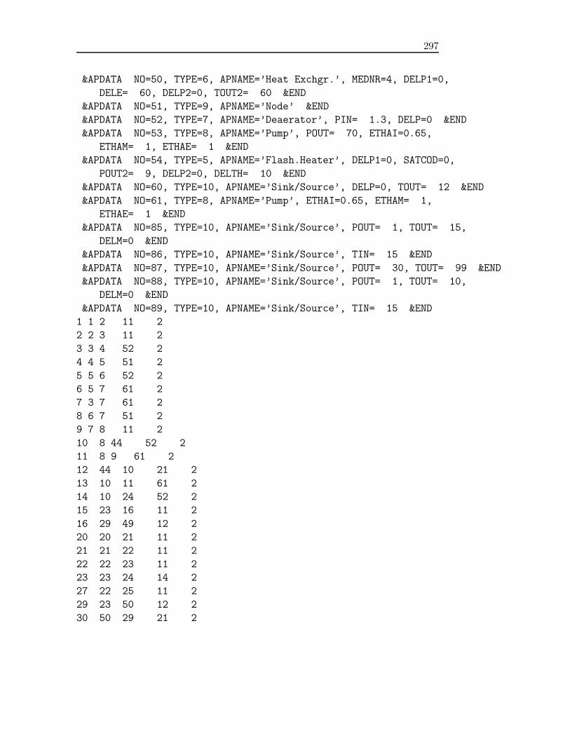
297
&APDATA NO=50, TYPE=6, APNAME=’Heat Exchgr.’, MEDNR=4, DELP1=0,
DELE= 60, DELP2=0, TOUT2= 60 &END
&APDATA NO=51, TYPE=9, APNAME=’Node’ &END
&APDATA NO=52, TYPE=7, APNAME=’Deaerator’, PIN= 1.3, DELP=0 &END
&APDATA NO=53, TYPE=8, APNAME=’Pump’, POUT= 70, ETHAI=0.65,
ETHAM= 1, ETHAE= 1 &END
&APDATA NO=54, TYPE=5, APNAME=’Flash.Heater’, DELP1=0, SATCOD=0,
POUT2= 9, DELP2=0, DELTH= 10 &END
&APDATA NO=60, TYPE=10, APNAME=’Sink/Source’, DELP=0, TOUT= 12 &END
&APDATA NO=61, TYPE=8, APNAME=’Pump’, ETHAI=0.65, ETHAM= 1,
ETHAE= 1 &END
&APDATA NO=85, TYPE=10, APNAME=’Sink/Source’, POUT= 1, TOUT= 15,
DELM=0 &END
&APDATA NO=86, TYPE=10, APNAME=’Sink/Source’, TIN= 15 &END
&APDATA NO=87, TYPE=10, APNAME=’Sink/Source’, POUT= 30, TOUT= 99 &END
&APDATA NO=88, TYPE=10, APNAME=’Sink/Source’, POUT= 1, TOUT= 10,
DELM=0 &END
&APDATA NO=89, TYPE=10, APNAME=’Sink/Source’, TIN= 15 &END
1 1 2 11 2
2 2 3 11 2
3 3 4 52 2
4 4 5 51 2
5 5 6 52 2
6 5 7 61 2
7 3 7 61 2
8 6 7 51 2
9 7 8 11 2
10 8 44 52 2
11 8 9 61 2
12 44 10 21 2
13 10 11 61 2
14 10 24 52 2
15 23 16 11 2
16 29 49 12 2
20 20 21 11 2
21 21 22 11 2
22 22 23 11 2
23 23 24 14 2
27 22 25 11 2
29 23 50 12 2
30 50 29 21 2
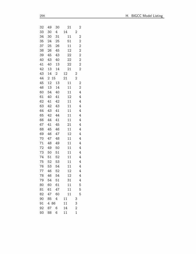
298 H. BIGCC Model Listing
32 49 30 21 2
33 30 4 14 2
34 30 31 11 2
35 24 25 51 2
37 25 26 11 2
38 26 45 12 2
39 45 43 22 2
40 43 40 22 2
41 40 13 22 2
42 13 14 21 2
43 14 2 12 2
44 2 15 21 2
45 12 13 11 2
46 13 14 11 2
60 54 40 11 4
61 40 41 12 4
62 41 42 11 4
63 42 43 11 4
64 43 41 11 4
65 42 44 11 4
66 44 41 11 4
67 41 45 21 4
68 45 46 11 4
69 46 47 12 4
70 47 48 11 4
71 48 49 11 4
72 49 50 11 4
73 50 51 11 4
74 51 52 11 4
75 52 53 11 4
76 53 54 11 4
77 46 52 12 4
78 46 54 12 4
79 54 51 31 4
80 60 61 11 5
81 61 47 11 5
82 47 60 11 5
90 85 4 11 3
91 4 86 11 3
92 87 6 14 2
93 88 6 11 1
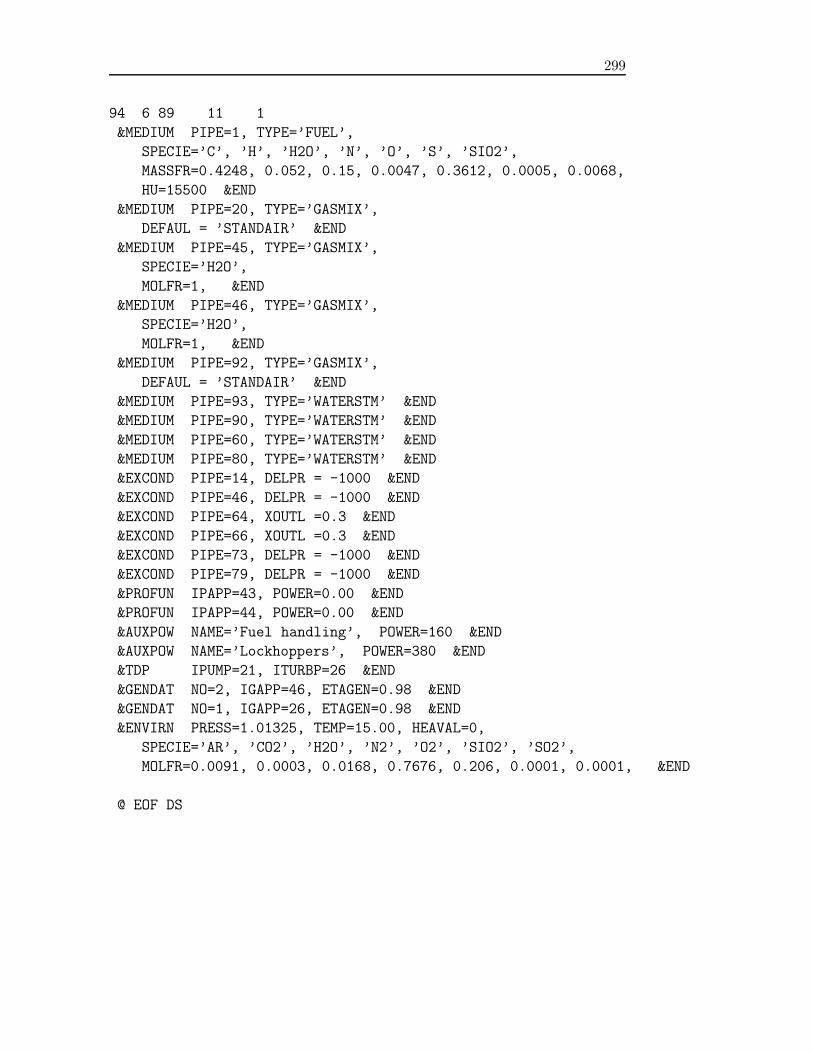
299
94 6 89 11 1
&MEDIUM PIPE=1, TYPE=’FUEL’,
SPECIE=’C’, ’H’, ’H2O’, ’N’, ’O’, ’S’, ’SIO2’,
MASSFR=0.4248, 0.052, 0.15, 0.0047, 0.3612, 0.0005, 0.0068,
HU=15500 &END
&MEDIUM PIPE=20, TYPE=’GASMIX’,
DEFAUL = ’STANDAIR’ &END
&MEDIUM PIPE=45, TYPE=’GASMIX’,
SPECIE=’H2O’,
MOLFR=1, &END
&MEDIUM PIPE=46, TYPE=’GASMIX’,
SPECIE=’H2O’,
MOLFR=1, &END
&MEDIUM PIPE=92, TYPE=’GASMIX’,
DEFAUL = ’STANDAIR’ &END
&MEDIUM PIPE=93, TYPE=’WATERSTM’ &END
&MEDIUM PIPE=90, TYPE=’WATERSTM’ &END
&MEDIUM PIPE=60, TYPE=’WATERSTM’ &END
&MEDIUM PIPE=80, TYPE=’WATERSTM’ &END
&EXCOND PIPE=14, DELPR = -1000 &END
&EXCOND PIPE=46, DELPR = -1000 &END
&EXCOND PIPE=64, XOUTL =0.3 &END
&EXCOND PIPE=66, XOUTL =0.3 &END
&EXCOND PIPE=73, DELPR = -1000 &END
&EXCOND PIPE=79, DELPR = -1000 &END
&PROFUN IPAPP=43, POWER=0.00 &END
&PROFUN IPAPP=44, POWER=0.00 &END
&AUXPOW NAME=’Fuel handling’, POWER=160 &END
&AUXPOW NAME=’Lockhoppers’, POWER=380 &END
&TDP IPUMP=21, ITURBP=26 &END
&GENDAT NO=2, IGAPP=46, ETAGEN=0.98 &END
&GENDAT NO=1, IGAPP=26, ETAGEN=0.98 &END
&ENVIRN PRESS=1.01325, TEMP=15.00, HEAVAL=0,
SPECIE=’AR’, ’CO2’, ’H2O’, ’N2’, ’O2’, ’SIO2’, ’SO2’,
MOLFR=0.0091, 0.0003, 0.0168, 0.7676, 0.206, 0.0001, 0.0001, &END
@ EOF DS

300 H. BIGCC Model Listing
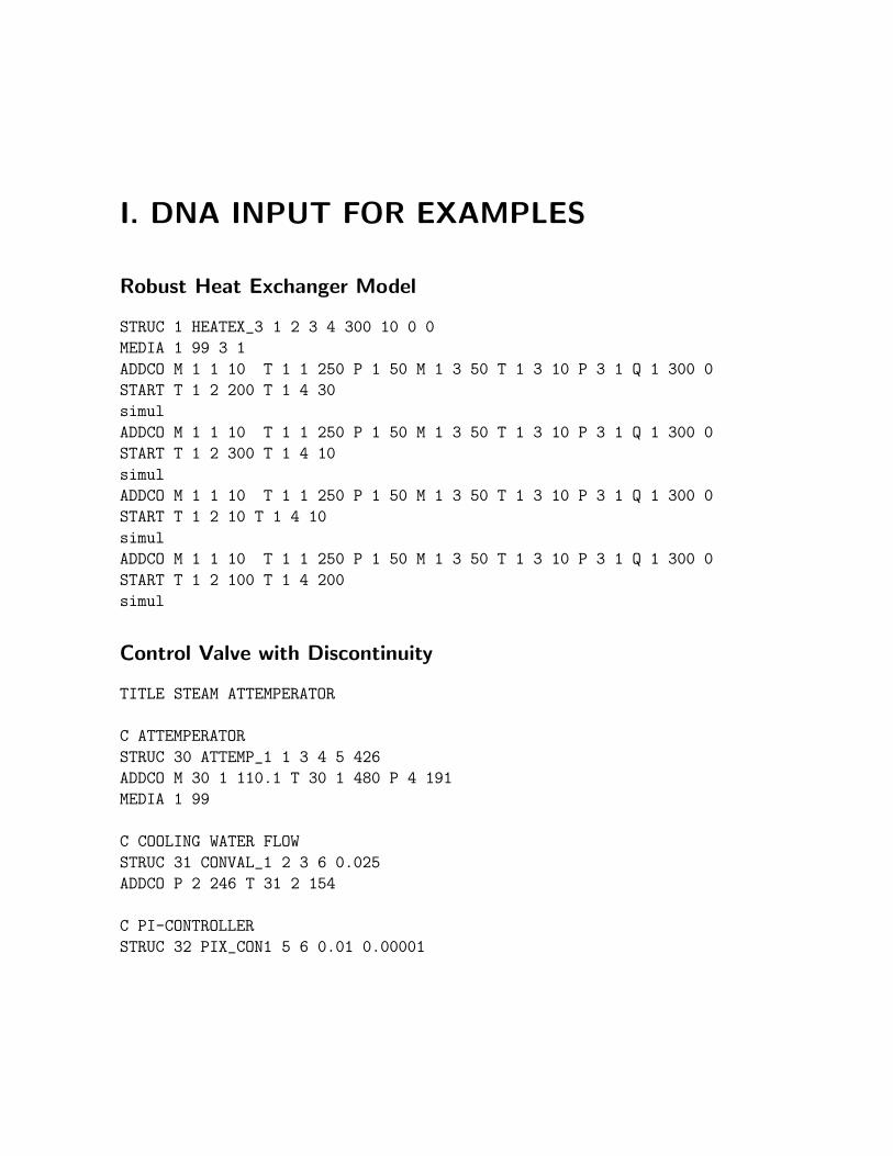
I. DNA INPUT FOR EXAMPLES
Robust Heat Exchanger Model
STRUC 1 HEATEX_3 1 2 3 4 300 10 0 0
MEDIA 1 99 3 1
ADDCO M 1 1 10 T 1 1 250 P 1 50 M 1 3 50 T 1 3 10 P 3 1 Q 1 300 0
START T 1 2 200 T 1 4 30
simul
ADDCO M 1 1 10 T 1 1 250 P 1 50 M 1 3 50 T 1 3 10 P 3 1 Q 1 300 0
START T 1 2 300 T 1 4 10
simul
ADDCO M 1 1 10 T 1 1 250 P 1 50 M 1 3 50 T 1 3 10 P 3 1 Q 1 300 0
START T 1 2 10 T 1 4 10
simul
ADDCO M 1 1 10 T 1 1 250 P 1 50 M 1 3 50 T 1 3 10 P 3 1 Q 1 300 0
START T 1 2 100 T 1 4 200
simul
Control Valve with Discontinuity
TITLE STEAM ATTEMPERATOR
C ATTEMPERATOR
STRUC 30 ATTEMP_1 1 3 4 5 426
ADDCO M 30 1 110.1 T 30 1 480 P 4 191
MEDIA 1 99
C COOLING WATER FLOW
STRUC 31 CONVAL_1 2 3 6 0.025
ADDCO P 2 246 T 31 2 154
C PI-CONTROLLER
STRUC 32 PIX_CON1 5 6 0.01 0.00001
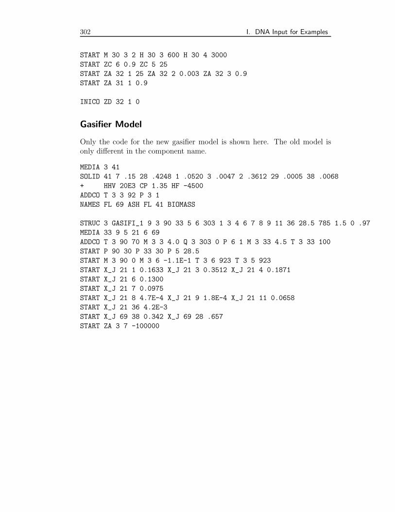
302 I. DNA Input for Examples
START M 30 3 2 H 30 3 600 H 30 4 3000
START ZC 6 0.9 ZC 5 25
START ZA 32 1 25 ZA 32 2 0.003 ZA 32 3 0.9
START ZA 31 1 0.9
INICO ZD 32 1 0
Gasifier Model
Only the code for the new gasifier model is shown here. The old model isonly different in the component name.
MEDIA 3 41
SOLID 41 7 .15 28 .4248 1 .0520 3 .0047 2 .3612 29 .0005 38 .0068
+ HHV 20E3 CP 1.35 HF -4500
ADDCO T 3 3 92 P 3 1
NAMES FL 69 ASH FL 41 BIOMASS
STRUC 3 GASIFI_1 9 3 90 33 5 6 303 1 3 4 6 7 8 9 11 36 28.5 785 1.5 0 .97
MEDIA 33 9 5 21 6 69
ADDCO T 3 90 70 M 3 3 4.0 Q 3 303 0 P 6 1 M 3 33 4.5 T 3 33 100
START P 90 30 P 33 30 P 5 28.5
START M 3 90 0 M 3 6 -1.1E-1 T 3 6 923 T 3 5 923
START X_J 21 1 0.1633 X_J 21 3 0.3512 X_J 21 4 0.1871
START X_J 21 6 0.1300
START X_J 21 7 0.0975
START X_J 21 8 4.7E-4 X_J 21 9 1.8E-4 X_J 21 11 0.0658
START X_J 21 36 4.2E-3
START X_J 69 38 0.342 X_J 69 28 .657
START ZA 3 7 -100000


