Embed Size (px)
Citation preview
5/12/2018 GetTRDoc - slidepdf.com
http://slidepdf.com/reader/full/gettrdoc-55a35d023bc26 1/116
NAVAL
POSTGRADUATE
SCHOOLMONTEREY, CALIFORNIA
THESIS
Approved for public release; distribution is unlimited
DESIGN AND IMPLEMENTATION OF A MOBILE PHONE
LOCATOR USING SOFTWARE DEFINED RADIO
by
Ian Paul Larsen
September 2007
Thesis Advisor: Frank E. Kragh
Second Reader: R. Clark Robertson

5/12/2018 GetTRDoc - slidepdf.com
http://slidepdf.com/reader/full/gettrdoc-55a35d023bc26 2/116
THIS PAGE INTENTIONALLY LEFT BLANK

5/12/2018 GetTRDoc - slidepdf.com
http://slidepdf.com/reader/full/gettrdoc-55a35d023bc26 3/116
REPORT DOCUMENTATION PAGE Form Approved OMB No. 0704-0188
Public reporting burden for this collection of information is estimated to average 1 hour per response, including the time for reviewing instruction,
searching existing data sources, gathering and maintaining the data needed, and completing and reviewing the collection of information. Send
comments regarding this burden estimate or any other aspect of this collection of information, including suggestions for reducing this burden, to
Washington headquarters Services, Directorate for Information Operations and Reports, 1215 Jefferson Davis Highway, Suite 1204, Arlington, VA
22202-4302, and to the Office of Management and Budget, Paperwork Reduction Project (0704-0188) Washington DC 20503.
1. AGENCY USE ONLY (Leave blank) 2. REPORT DATE
SEP 07
3. REPORT TYPE AND DATES COVERED
Master’s Thesis
4. TITLE AND SUBTITLE Design and Implementation of a Mobile Phone
Locator Using Software Defined Radio
6. AUTHOR(S) Ian Paul Larsen
5. FUNDING NUMBERS
7. PERFORMING ORGANIZATION NAME(S) AND ADDRESS(ES)
Naval Postgraduate School
Monterey, CA 93943-5000
8. PERFORMING ORGANIZATION
REPORT NUMBER
9. SPONSORING /MONITORING AGENCY NAME(S) AND ADDRESS(ES)
N/A
10. SPONSORING/MONITORING
AGENCY REPORT NUMBER
11. SUPPLEMENTARY NOTES The views expressed in this thesis are those of the author and do not reflect the official policy
or position of the Department of Defense or the U.S. Government.
12a. DISTRIBUTION / AVAILABILITY STATEMENT
Approved for public release; distribution is unlimited
12b. DISTRIBUTION CODE
13. ABSTRACT (maximum 200 words)
This thesis presents an approach for generating, detecting, and decoding a Global System for Mobile Communications
(GSM) signal using software defined radio and commodity computer hardware. Using software designed by the GNU free-
software project as a base, standard GSM packets were transmitted and received over the air, and their arrival times detected. A
method is provided to use software analysis of multiple receivers to locate an emitter based on the information received by the
software radio. Results and accuracy analysis as well as limitations are shown based on initial testing. Complete implementation
source code is provided in the appendices.
14. SUBJECT TERMS GSM, software defined radio, geolocation, mobile phone, time difference of
arrival
15. NUMBER OF
PAGES
116
16. PRICE CODE
17. SECURITY
CLASSIFICATION OF
REPORT
Unclassified
18. SECURITY
CLASSIFICATION OF THIS
PAGE
Unclassified
19. SECURITY
CLASSIFICATION OF
ABSTRACT
Unclassified
20. LIMITATION OF
ABSTRACT
UU
NSN 7540-01-280-5500 Standard Form 298 (Rev. 2-89)
Prescribed by ANSI Std. 239-18
i

5/12/2018 GetTRDoc - slidepdf.com
http://slidepdf.com/reader/full/gettrdoc-55a35d023bc26 4/116
THIS PAGE INTENTIONALLY LEFT BLANK
ii
5/12/2018 GetTRDoc - slidepdf.com
http://slidepdf.com/reader/full/gettrdoc-55a35d023bc26 5/116
Approved for public release; distribution is unlimited
DESIGN AND IMPLEMENTATION OF A MOBILE
PHONE LOCATOR USING SOFTWARE DEFINEDRADIO
Ian Paul LarsenLieutenant, United States Navy
B.S., United States Naval Academy, 2001
Submitted in partial fulfillment of therequirements for the degree of
MASTER OF SCIENCE IN ELECTRICAL ENGINEERING
from the
NAVAL POSTGRADUATE SCHOOL
September 2007
Author: Ian Paul Larsen
Approved by: Frank E. KraghThesis Advisor
R. Clark Robertson
Second Reader
Jeffrey B. KnorrChairman, Department of Electrical and Computer Engineering
iii

5/12/2018 GetTRDoc - slidepdf.com
http://slidepdf.com/reader/full/gettrdoc-55a35d023bc26 6/116
THIS PAGE INTENTIONALLY LEFT BLANK
iv
5/12/2018 GetTRDoc - slidepdf.com
http://slidepdf.com/reader/full/gettrdoc-55a35d023bc26 7/116
ABSTRACT
This thesis presents an approach for generating, detecting, and decoding a
Global System for Mobile communications (GSM) signal using software defined ra-
dio and commodity computer hardware. Using software designed by the GNU free-
software project as a base, standard GSM packets were transmitted and received over
the air and their arrival times detected. A method is provided to use software analysis
of multiple receivers to locate an emitter based on the information received by the
software radio. Results and accuracy as well as limitations are shown based on initial
testing. Complete implementation source code is provided in the appendices.
v

5/12/2018 GetTRDoc - slidepdf.com
http://slidepdf.com/reader/full/gettrdoc-55a35d023bc26 8/116
THIS PAGE INTENTIONALLY LEFT BLANK
vi
5/12/2018 GetTRDoc - slidepdf.com
http://slidepdf.com/reader/full/gettrdoc-55a35d023bc26 9/116
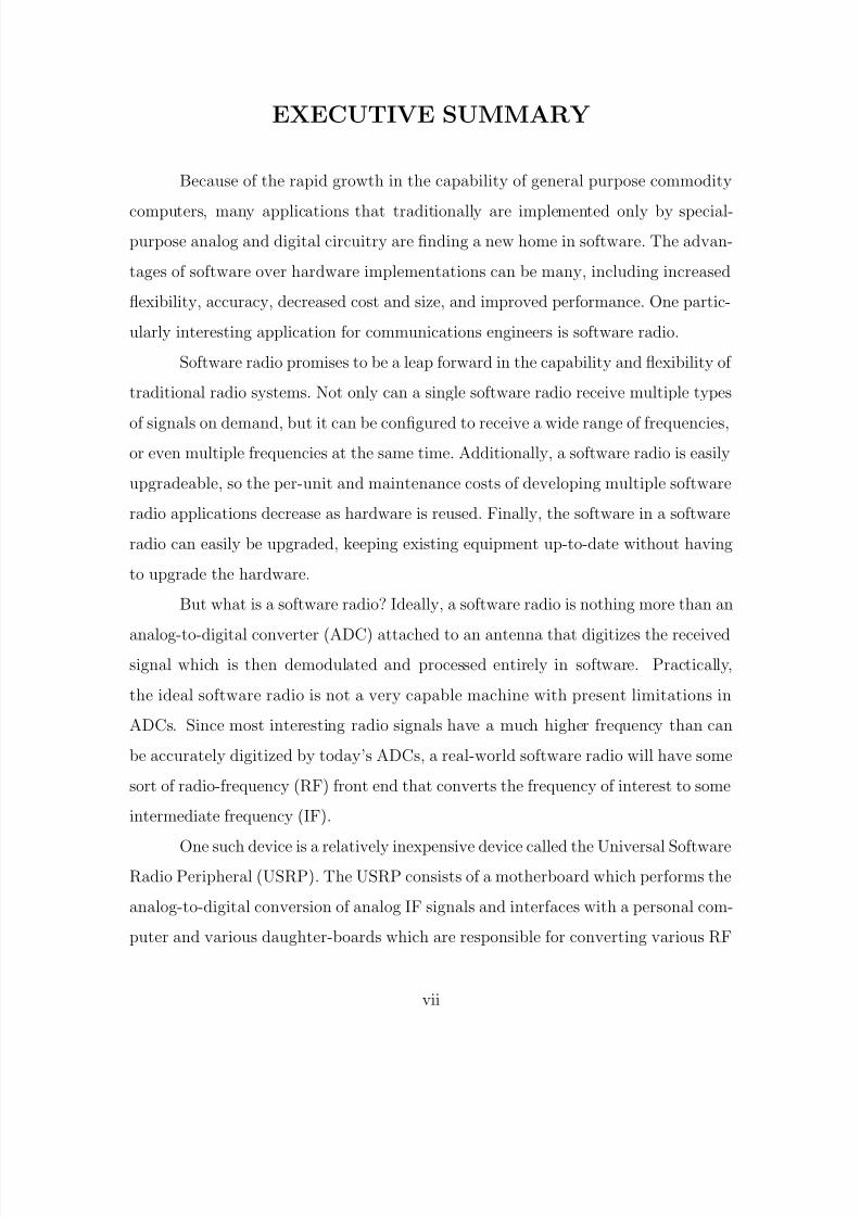
EXECUTIVE SUMMARY
Because of the rapid growth in the capability of general purpose commodity
computers, many applications that traditionally are implemented only by special-
purpose analog and digital circuitry are finding a new home in software. The advan-
tages of software over hardware implementations can be many, including increased
flexibility, accuracy, decreased cost and size, and improved performance. One partic-
ularly interesting application for communications engineers is software radio.
Software radio promises to be a leap forward in the capability and flexibility of
traditional radio systems. Not only can a single software radio receive multiple types
of signals on demand, but it can be configured to receive a wide range of frequencies,or even multiple frequencies at the same time. Additionally, a software radio is easily
upgradeable, so the per-unit and maintenance costs of developing multiple software
radio applications decrease as hardware is reused. Finally, the software in a software
radio can easily be upgraded, keeping existing equipment up-to-date without having
to upgrade the hardware.
But what is a software radio? Ideally, a software radio is nothing more than an
analog-to-digital converter (ADC) attached to an antenna that digitizes the receivedsignal which is then demodulated and processed entirely in software. Practically,
the ideal software radio is not a very capable machine with present limitations in
ADCs. Since most interesting radio signals have a much higher frequency than can
be accurately digitized by today’s ADCs, a real-world software radio will have some
sort of radio-frequency (RF) front end that converts the frequency of interest to some
intermediate frequency (IF).
One such device is a relatively inexpensive device called the Universal SoftwareRadio Peripheral (USRP). The USRP consists of a motherboard which performs the
analog-to-digital conversion of analog IF signals and interfaces with a personal com-
puter and various daughter-boards which are responsible for converting various RF
vii
5/12/2018 GetTRDoc - slidepdf.com
http://slidepdf.com/reader/full/gettrdoc-55a35d023bc26 10/116
frequencies to IF and sending that analog IF signal to the motherboard. This makes
the USRP extremely flexible, as different daughter-boards can be used depending on
the frequency of interest. A side benefit is that most of the important functional-
ity can implemented in a single motherboard, making the multiple daughter-boards
inexpensive devices.
A signal that is particularly interesting is that used by mobile phones that
comply with the Global Systems for Mobile communication (GSM) standard. Used
globally, it is the most popular standard for mobile phones. It has a number of features
that make receiving the signal challenging for a software radio, such as time-division
multiplexing combined with slow frequency-hopping. However, the GSM standard is
freely available and, as such, anyone with the ability and inclination to implement
the standard in software can produce a conforming GSM software radio.
One of the primary problems in Information Warfare (IW) and signals intel-
ligence is finding the location of the emitter of a signal. There are many methods
to accomplish this task with various accuracy and complexity. One such method is
to use multiple receivers in different locations and to measure the difference in time
between when the signal was received at one receiver compared with another. This
is called time-difference-of-arrival (TDOA) and has been successfully implemented in
the past in hardware.
This thesis examines the feasibility of implementing a system for locating an
emitter of a GSM signal using the TDOA method with software radio and the USRP.
In order to accomplish this, the objectives of this research were as follows:
• Generate a typical packet of GSM traffic that is as close to mathematicallyperfect as possible.
• Transmit the GSM packet using software radio.
• Receive the GSM packet using software radio.
• Partially demodulate the GSM packet in software.
• Determine the time-of-arrival of the GSM packet.
viii
5/12/2018 GetTRDoc - slidepdf.com
http://slidepdf.com/reader/full/gettrdoc-55a35d023bc26 11/116
• Perform a statistical analysis of the feasibility of performing geolocation withsoftware radio.
These objectives were all completed with varying degrees of success due to
limitations in software radio itself, the performance of general purpose computer
hardware, and time.
The generation of the GSM signal in software was performed after careful
analysis of the GSM specification, with special attention paid to the accuracy of the
signal. Once the signal had been generated, it was sent repeatedly using the GNU
Radio software and the USRP, so that the timing of the signal could be measured by
the receiver.
A receiver was implemented in software that would take data from the USRPand demodulate it to the point where the arrival time could be measured. Partial
demodulation of the digital data in the signal was sufficient for the arrival time
measurement, so complete demodulation was not implemented. Subsequent to the
demodulation, a software correlator was used to compare the received data with an
ideal target sample in order to determine (within the accuracy of one digital sample)
when the signal was received. This time data was checked against the known time of
transmission and analyzed for accuracy.The research found that implementing a TDOA software radio system is en-
tirely feasible. However, significant portions of the implementation must make use of
faster hardware like field-programmable gate arrays (FPGA) in order to perform the
calculations in real-time. Precision of the location calculation using general purpose
hardware and the USRP was on the range of 35-100 meters, with the accuracy being
± 35-100 meters more than 90% of the time. Precision and accuracy were heavily
dependent on the speed of the personal computer involved in the reception of thesignal.
ix

5/12/2018 GetTRDoc - slidepdf.com
http://slidepdf.com/reader/full/gettrdoc-55a35d023bc26 12/116
THIS PAGE INTENTIONALLY LEFT BLANK
x

5/12/2018 GetTRDoc - slidepdf.com
http://slidepdf.com/reader/full/gettrdoc-55a35d023bc26 13/116
DISCLAIMER
The computer source code in the Appendices is supplied on an “as is” basis,
with no warranties of any kind. The author bears no responsibility for any conse-
quences of using these programs.
xi

5/12/2018 GetTRDoc - slidepdf.com
http://slidepdf.com/reader/full/gettrdoc-55a35d023bc26 14/116
THIS PAGE INTENTIONALLY LEFT BLANK
xii
5/12/2018 GetTRDoc - slidepdf.com
http://slidepdf.com/reader/full/gettrdoc-55a35d023bc26 15/116
TABLE OF CONTENTS
I. INTRODUCTION . . . . . . . . . . . . . . . . . . . . . . . . . . . . 1
A. BACKGROUND . . . . . . . . . . . . . . . . . . . . . . . . . . 1
B. OBJECTIVE AND APPROACH . . . . . . . . . . . . . . . . . 2
C. RELATED WORK . . . . . . . . . . . . . . . . . . . . . . . . . 3
D. THESIS ORGANIZATION . . . . . . . . . . . . . . . . . . . . . 3
II. ANALYSIS . . . . . . . . . . . . . . . . . . . . . . . . . . . . . . . . 5
A. GLOBAL SYSTEM FOR MOBILE COMMUNICATION . . . . 5
1. GSM Bursts . . . . . . . . . . . . . . . . . . . . . . . . . 5
2. GSM Frequency-Hopping . . . . . . . . . . . . . . . . . . 73. GSM Channel Definition . . . . . . . . . . . . . . . . . . 8
B. GSM MODULATION . . . . . . . . . . . . . . . . . . . . . . . 9
1. Differential Encoding . . . . . . . . . . . . . . . . . . . . 10
2. GMSK Filtering . . . . . . . . . . . . . . . . . . . . . . . 10
C. THE UNIVERSAL SOFTWARE RADIO PERIPHERAL . . . . 12
1. Receive Capabilities . . . . . . . . . . . . . . . . . . . . . 12
2. Transmit Capabilities . . . . . . . . . . . . . . . . . . . . 163. Data Transfer Capabilities . . . . . . . . . . . . . . . . . 17
D. SIGNAL DETECTION . . . . . . . . . . . . . . . . . . . . . . . 18
1. Correlator . . . . . . . . . . . . . . . . . . . . . . . . . . 18
E. GEOLOCATION . . . . . . . . . . . . . . . . . . . . . . . . . . 19
1. Requirements . . . . . . . . . . . . . . . . . . . . . . . . 19
2. Precision . . . . . . . . . . . . . . . . . . . . . . . . . . . 20
3. Limitations and Workarounds . . . . . . . . . . . . . . . 20F. CONCLUSION . . . . . . . . . . . . . . . . . . . . . . . . . . . 22
III. IMPLEMENTATION . . . . . . . . . . . . . . . . . . . . . . . . . . 23
A. GMSK SIGNAL GENERATION . . . . . . . . . . . . . . . . . 23
xiii
5/12/2018 GetTRDoc - slidepdf.com
http://slidepdf.com/reader/full/gettrdoc-55a35d023bc26 16/116
1. GMSK Filter Implementation . . . . . . . . . . . . . . . 23
2. Determining the Sample Rate . . . . . . . . . . . . . . . 24
3. Baseband Signal Generation . . . . . . . . . . . . . . . . 25
4. Application of a GMSK Filter . . . . . . . . . . . . . . . 27
B. GMSK DECODING . . . . . . . . . . . . . . . . . . . . . . . . 29
1. FM Demodulation . . . . . . . . . . . . . . . . . . . . . . 29
2. Determining Sample Rate . . . . . . . . . . . . . . . . . 31
3. Generating Target Sequence . . . . . . . . . . . . . . . . 32
4. Correlation . . . . . . . . . . . . . . . . . . . . . . . . . . 32
5. Storage Requirements . . . . . . . . . . . . . . . . . . . . 33
C. CONCLUSION . . . . . . . . . . . . . . . . . . . . . . . . . . . 34
IV. EXPERIMENTATION . . . . . . . . . . . . . . . . . . . . . . . . . 35
A. SET UP . . . . . . . . . . . . . . . . . . . . . . . . . . . . . . . 35
B. TRANSMISSION . . . . . . . . . . . . . . . . . . . . . . . . . . 36
C. RECEPTION . . . . . . . . . . . . . . . . . . . . . . . . . . . . 36
1. Initial Results . . . . . . . . . . . . . . . . . . . . . . . . 36
2. Signal-to-Noise Ratio . . . . . . . . . . . . . . . . . . . . 38
D. CORRELATION . . . . . . . . . . . . . . . . . . . . . . . . . . 39
1. Algorithm . . . . . . . . . . . . . . . . . . . . . . . . . . 39
2. Results . . . . . . . . . . . . . . . . . . . . . . . . . . . . 41
3. Software Radio Limitations . . . . . . . . . . . . . . . . . 43
E. LOCATING THE EMITTER . . . . . . . . . . . . . . . . . . . 44
F. CONCLUSION . . . . . . . . . . . . . . . . . . . . . . . . . . . 47
V. CONCLUSION . . . . . . . . . . . . . . . . . . . . . . . . . . . . . . 49
A. CONCLUSIONS . . . . . . . . . . . . . . . . . . . . . . . . . . 49
B. RECOMMENDATIONS . . . . . . . . . . . . . . . . . . . . . . 49
APPENDIX A. CORRELATION DATA . . . . . . . . . . . . . . . . . 51
xiv
5/12/2018 GetTRDoc - slidepdf.com
http://slidepdf.com/reader/full/gettrdoc-55a35d023bc26 17/116
APPENDIX B. UNDERSTANDING COMMON LISP EXAMPLES 55
1. S-EXPRESSIONS . . . . . . . . . . . . . . . . . . . . . . . . . . 55
APPENDIX C. GMSK.LISP . . . . . . . . . . . . . . . . . . . . . . . . . 59
APPENDIX D. TRANSMIT.PY . . . . . . . . . . . . . . . . . . . . . . 65
APPENDIX E. RECEIVE.PY . . . . . . . . . . . . . . . . . . . . . . . . 67
APPENDIX F. RECEIVE2.PY . . . . . . . . . . . . . . . . . . . . . . . 69
APPENDIX G. FM DEMOD.PL . . . . . . . . . . . . . . . . . . . . . . 71
APPENDIX H. CORRELATOR.CPP . . . . . . . . . . . . . . . . . . . 75
APPENDIX I. STATISTICS.PL . . . . . . . . . . . . . . . . . . . . . . . 81
APPENDIX J. DISTANCE.LISP . . . . . . . . . . . . . . . . . . . . . . 83
LIST OF REFERENCES . . . . . . . . . . . . . . . . . . . . . . . . . . . 87
INITIAL DISTRIBUTION LIST . . . . . . . . . . . . . . . . . . . . . . 89
xv

5/12/2018 GetTRDoc - slidepdf.com
http://slidepdf.com/reader/full/gettrdoc-55a35d023bc26 18/116
THIS PAGE INTENTIONALLY LEFT BLANK
xvi
5/12/2018 GetTRDoc - slidepdf.com
http://slidepdf.com/reader/full/gettrdoc-55a35d023bc26 19/116
LIST OF FIGURES
Figure 1. Illustration of a frequency-hopping GSM channel. . . . . . . . . 9
Figure 2. Illustration of aliasing due to down-sampling. . . . . . . . . . . . 16
Figure 3. Complex FM baseband signal from −10 to 10 Hz. . . . . . . . . 27
Figure 4. GSM access burst. . . . . . . . . . . . . . . . . . . . . . . . . . . 28
Figure 5. Gaussian filtered GSM access burst synchronization sequence. . 28
Figure 6. Modulated access burst, I and Q channels. . . . . . . . . . . . . 29
Figure 7. Two successive FM samples. . . . . . . . . . . . . . . . . . . . . 30
Figure 8. Target GSM synchronization sequence. . . . . . . . . . . . . . . 33
Figure 9. Demodulated GMSK signal, no power measuring. . . . . . . . . 37Figure 10. Demodulated GMSK signal, repeated bursts. . . . . . . . . . . . 38
Figure 11. Demodulated GMSK signal, single burst. . . . . . . . . . . . . . 39
Figure 12. Result of correlation with target sequence. . . . . . . . . . . . . 40
Figure 13. Algorithmic jitter in correlator. . . . . . . . . . . . . . . . . . . 41
Figure 14. Histogram of sample errors based on 5101 data points. . . . . . 41
Figure 15. Emitter location with one-meter precision. . . . . . . . . . . . . 46
Figure 16. Emitter location with 37-meter precision. . . . . . . . . . . . . . 47
xvii

5/12/2018 GetTRDoc - slidepdf.com
http://slidepdf.com/reader/full/gettrdoc-55a35d023bc26 20/116
THIS PAGE INTENTIONALLY LEFT BLANK
xviii
5/12/2018 GetTRDoc - slidepdf.com
http://slidepdf.com/reader/full/gettrdoc-55a35d023bc26 21/116
LIST OF TABLES
Table 1. Fields of a GSM access burst. . . . . . . . . . . . . . . . . . . . 6
Table 2. Access burst synchronization sequences. . . . . . . . . . . . . . . 8
Table 3. Transmitting computer settings. . . . . . . . . . . . . . . . . . . 35
Table 4. Receiving computer settings. . . . . . . . . . . . . . . . . . . . . 35
Table 5. Correlation output data. . . . . . . . . . . . . . . . . . . . . . . 42
Table 6. Correlation statistics for six second reception. . . . . . . . . . . 42
xix

5/12/2018 GetTRDoc - slidepdf.com
http://slidepdf.com/reader/full/gettrdoc-55a35d023bc26 22/116
THIS PAGE INTENTIONALLY LEFT BLANK
xx
5/12/2018 GetTRDoc - slidepdf.com
http://slidepdf.com/reader/full/gettrdoc-55a35d023bc26 23/116
TABLE OF ACRONYMS
NPS Naval Postgraduate School
GSM Global System for Mobile communicationUSRP Universal Software Radio PeripheralIW Information Warfare
TDOA Time-Difference-of-ArrivalFPGA Field Programmable Gate Array
DSP Digital Signal ProcessorCPU Central Processing UnitPC Personal Computer
JTRS Joint Tactical Radio SystemSCA Software Communication Architecture
OSSIE Open Source SCA Implementation::Embedded
ADC Analog-to-Digital ConverterDAC Digital-to-Analog ConverterDDC Digital Down-ConverterGNU Gnu’s Not Unix
IF Intermediate FrequencyRF Radio FrequencyFM Frequency Modulation
GMSK Gaussian Minimum-Shift KeyingPGA Programmable Gain AmplifierCIC Casaded Integrator-CombUSN Universal Serial BusNCO Numerically Controlled OscillatorSNR Signal to Noise Ratio
xxi

5/12/2018 GetTRDoc - slidepdf.com
http://slidepdf.com/reader/full/gettrdoc-55a35d023bc26 24/116
THIS PAGE INTENTIONALLY LEFT BLANK
xxii
5/12/2018 GetTRDoc - slidepdf.com
http://slidepdf.com/reader/full/gettrdoc-55a35d023bc26 25/116
ACKNOWLEDGMENTS
I would like to thank the faculty members of the Naval Postgraduate School
for their assistance with this thesis, many of whom went above and beyond the call
of duty to assist me with my research, particularly my thesis adviser, Professor Frank
Kragh, Donna Miller, Bob Broadston, Jeff Knight, and my second reader Professor
Clark Robertson.
Also thank you to the members of the OSSIE team at Virginia Tech and the
members of the GNU Radio project, both for producing the excellent software that
made my research possible and for providing answers and guidance for my technical
questions.My sincerest thanks go to my wife Valarie who spent many long days at home
taking excellent care of my two beautiful daughters Amelia and Evangeline while I
was at school. Without her patience, help, and lunch deliveries this would not have
been possible.
xxiii

5/12/2018 GetTRDoc - slidepdf.com
http://slidepdf.com/reader/full/gettrdoc-55a35d023bc26 26/116
THIS PAGE INTENTIONALLY LEFT BLANK
xxiv
5/12/2018 GetTRDoc - slidepdf.com
http://slidepdf.com/reader/full/gettrdoc-55a35d023bc26 27/116
I. INTRODUCTION
A. BACKGROUND
Software defined radio, a relatively new field, promises to be a leap forward inthe capability and flexibility of traditional radio systems. Instead of producing com-
plex and inflexible analog hardware, a software radio tries to accomplish the same task
in the digital domain using reconfigurable hardware such as field programmable gate
arrays (FPGA), digital signal processors (DSP), or even general purpose processors
such as those found in a personal computer. Although there are many advantages to
processing radio signals in software, such as ease of manufacture and maintenance, the
performance of software components, particularly the flexible general purpose proces-sors, are just beginning to become powerful enough to handle the extraordinarily high
data rates required for some applications. [1]
One particularly demanding application of a radio receiver is geolocation, or
finding the location of the emitter of a signal based on the characteristics of the re-
ceived signal. Performing geolocation with any reasonable degree of accuracy requires
extremely sensitive and well-tuned equipment that can measure very small variations
in receive time and frequency. [2]But what is software defined radio, exactly? The term encompasses a lot of
technologies and techniques, so an example of an ideal software defined radio will give
the clearest understanding of what software radio is in general. An ideal software radio
is an antenna attached directly to an analog-to-digital converter (ADC) that samples
the signal coming in from the antenna. All subsequent demodulation, processing and
decoding of the signal are done by software in the discrete digital domain. [1]
For various reasons, not the least of which is that the hardware required foran ideal software defined radio would be costly, practical software radios vary slightly
from the ideal, whether by including special purpose hardware to perform demodu-
lation or an analog radio-frequency (RF) front-end that converts the high radio fre-
1
5/12/2018 GetTRDoc - slidepdf.com
http://slidepdf.com/reader/full/gettrdoc-55a35d023bc26 28/116
quency signal to an intermediate frequency that is more easily sampled by an ADC.
This allows the system to trade some flexibility for performance and practicality. [1]
Before this research was done, there was some doubt as to the ability of low-
cost, consumer-grade hardware to perform geolocation using software defined radio
and no hard data on how accurate it could be in practice. This research performs a
theoretical analysis of how accurate such software should be, and experimental results
show how well the theory corresponds to reality in practice.
B. OBJECTIVE AND APPROACH
The objectives of this research were to:
• Generate a typical packet of GSM traffic that is as close to mathematicallyperfect as possible.
• Transmit the GSM packet using software radio.
• Receive the GSM packet using software radio.
• Partially demodulate the GSM packet in software.
• Determine the time of arrival of the GSM packet.
•Perform an analysis of the feasibility of performing geolocation with software
radio.
To accomplish these objectives, it was necessary to calculate a discrete time
signal prior to any transmission. Next, software and the USRP were used to send
and receive the previously calculated and stored signal in real time and store the raw
incoming data on the receiving computer. Finally, the raw data was analyzed by
additional software to demodulate the signal and determine its time-of-arrival.
A number of different computer languages were used depending on the specific
purpose of the software component. A Common Lisp environment called CLISP was
chosen for the generation of the signal due to its native support of complex numbers,
2
5/12/2018 GetTRDoc - slidepdf.com
http://slidepdf.com/reader/full/gettrdoc-55a35d023bc26 29/116
high degree of mathematical precision, and ability to concisely implement mathemat-
ical algorithms. The GNU Radio free software project provided the libraries neces-
sary to communicate directly with the USRP with very little overhead, and various
scripts were written with the Perl computer language to perform the demodulation of
a frequency modulated signal and handle translation of binary data into a readable
textual representation that the gnuplot plotting program could then show graphically
for further analysis.
C. RELATED WORK
The GNU Radio project is an open-source software defined radio project that
manages the design of the Universal Software Radio Peripheral and the low-level
libraries used for its operation, as well as a relatively high-level software radio com-
ponent system. Some of the GNU Radio software was used in this thesis.
The Open Source SCA Implementation Embedded (OSSIE) project is another
open-source software defined radio project that focuses on compatibility with the
Joint Tactical Radio System (JTRS) Software Communications Architecture (SCA).
It provides a number of useful and educational tools for development and analysis of
software radios.
Recently, many students at the Naval Postgraduate School (NPS) have writ-
ten theses on either software defined radio or geolocation, including software radio
designs for various standards such as Interim Standard 95B (IS-95B) and Institute
of Electrical and Electronics Engineers (IEEE) 802.16 and 802.11a, software radio
designs for general binary frequency shift keyed signals, and geolocation using the
complex ambiguity function [3, 4, 5, 6, 7, 8].
D. THESIS ORGANIZATION
The body of this thesis is divided into four chapters in order to indicate the
level of technical detail. Chapter II focuses on general information about software
3
5/12/2018 GetTRDoc - slidepdf.com
http://slidepdf.com/reader/full/gettrdoc-55a35d023bc26 30/116
radio and GSM signals, and then discusses in specific theoretical detail how GSM and
software radio work. Chapter III shows how the mathematical analysis can be put
into practice by discussing the specific algorithms used to allow the software radio to
transmit and receive a Gaussian minimum-shift-keyed (GMSK) signal. Chapter IV
shows the results of that implementation, with graphs of the actual received signal
and an analysis of the accuracy with which it was detected.
4
5/12/2018 GetTRDoc - slidepdf.com
http://slidepdf.com/reader/full/gettrdoc-55a35d023bc26 31/116
II. ANALYSIS
A. GLOBAL SYSTEM FOR MOBILE COMMUNICATION
The Global System for Mobile communication (GSM) is a worldwide standardfor mobile telephone communication. Receiving a typical GSM signal presents many
challenges due to the nature of the signal. In order to allow many simultaneous users,
GSM uses a combination of time-division multiple access (TDMA), frequency-division
multiple access (FDMA), and slow frequency-hopping. [9]
With TDMA, a channel is divided into time slots and a single recurring time
slot is assigned to each user. Users transmit and receive in rapid succession, so
the illusion is created that transmission and reception are occurring simultaneously.With FDMA, the total bandwidth available to a GSM provider is divided into many
frequency bands so that multiple time-division multiplexed channels can be used
simultaneously on different frequency bands. [9]
While this all seems simple enough, channels are not specified to use a given
frequency on a permanent basis. Instead, GSM uses a form of slow frequency-hopping
that means that the frequency for a user’s channel will change for different time
slots. In effect, this means a transmitting user will transmit on one frequency for theduration of a time slot, then change frequency according to a specified sequence and
transmit during the next time slot. The same system is used for reception and is
explained in greater detail below. [9]
1. GSM Bursts
GSM uses a TDMA scheme for allowing multiple users access to a single fre-
quency band. For a given frequency that is allocated in this manner, there are eight
time slots that may be dedicated to individual users. These eight time slots compose
a TDMA frame. [9: p. 215]
The basic unit of transmission in GSM is the burst. A burst is a transmission
that occurs within a single time slot at a specific frequency [9]. The length of a
5
5/12/2018 GetTRDoc - slidepdf.com
http://slidepdf.com/reader/full/gettrdoc-55a35d023bc26 32/116
burst in bits is typically 147 (not including some number of guard bits that are not
transmitted), however, there are shorter bursts of 87 bits that have a specific function
[10]. The duration of the time slot in bits is 156.25, which allows for a short guard
period to reduce interference with bursts starting in the next time slot [10].
There are many different types of GSM bursts, and each has a different in-
formation content depending on the purpose of the burst [10]. A normal burst is
defined by the specification to carry voice and other data [10]. An access burst occurs
whenever the mobile user must gain access to the network, such as when the phone
is turned on, a call or text message is sent or received, or the user’s location changes
[9]. We are particularly interested in the access burst in this thesis due to the reasons
for which it occurs and the specific physical properties of the burst.
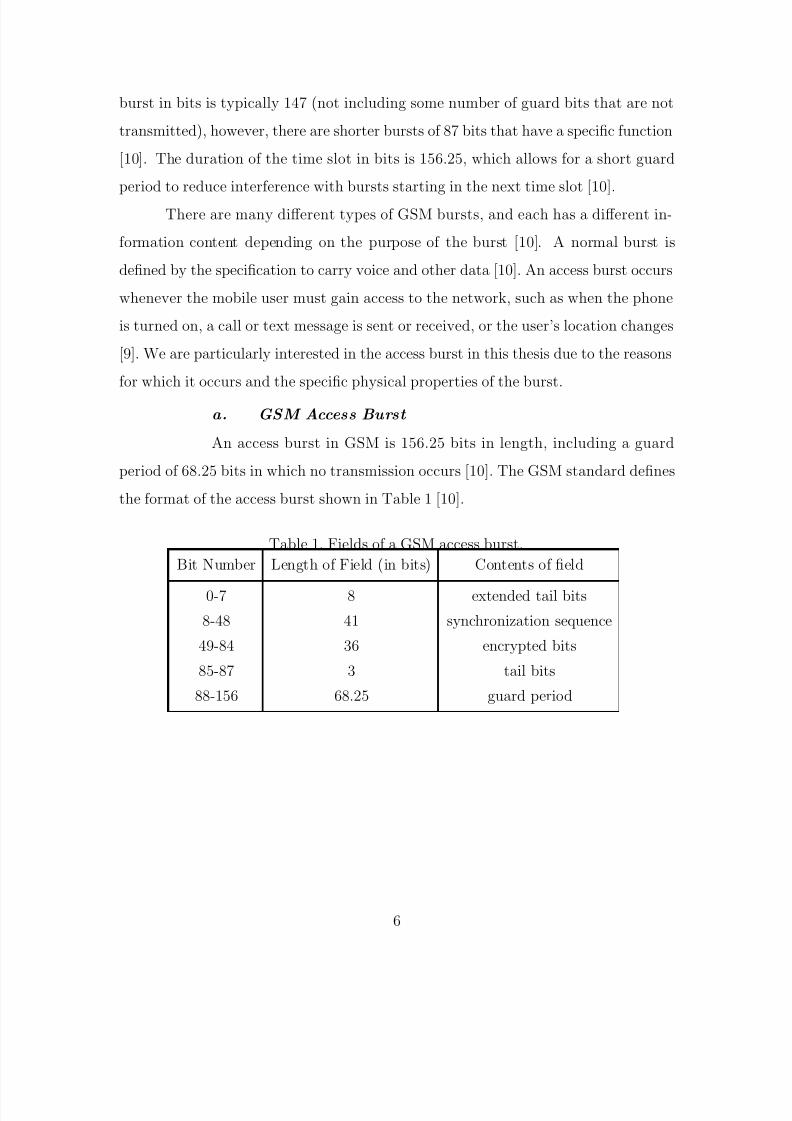
a. GSM Access Burst
An access burst in GSM is 156.25 bits in length, including a guard
period of 68.25 bits in which no transmission occurs [10]. The GSM standard defines
the format of the access burst shown in Table 1 [10].
Table 1. Fields of a GSM access burst.
Bit Number Length of Field (in bits) Contents of field
0-7 8 extended tail bits
8-48 41 synchronization sequence
49-84 36 encrypted bits
85-87 3 tail bits
88-156 68.25 guard period
6
5/12/2018 GetTRDoc - slidepdf.com
http://slidepdf.com/reader/full/gettrdoc-55a35d023bc26 33/116
b. Guard Period
The guard period is the portion of each GSM burst which is provided to
give the transmitter sufficient time to attenuate the transmitted signal. This period
is provided to allow for the fact that the beginning or ending of a transmission cannotoccur instantaneously, so the transient effect of the transmitter ramping up and down
occurs during this time. [10]
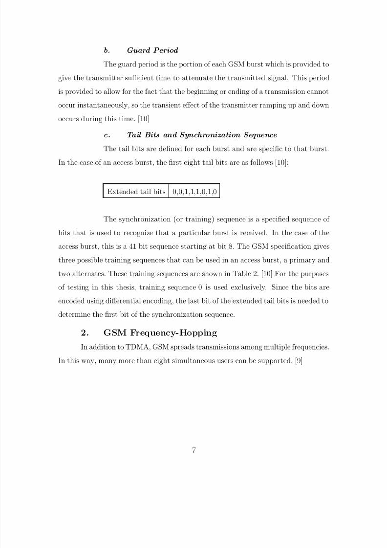
c. Tail Bits and Synchronization Sequence
The tail bits are defined for each burst and are specific to that burst.
In the case of an access burst, the first eight tail bits are as follows [10]:
Extended tail bits 0,0,1,1,1,0,1,0
The synchronization (or training) sequence is a specified sequence of
bits that is used to recognize that a particular burst is received. In the case of the
access burst, this is a 41 bit sequence starting at bit 8. The GSM specification gives
three possible training sequences that can be used in an access burst, a primary and
two alternates. These training sequences are shown in Table 2. [10] For the purposes
of testing in this thesis, training sequence 0 is used exclusively. Since the bits are
encoded using differential encoding, the last bit of the extended tail bits is needed to
determine the first bit of the synchronization sequence.
2. GSM Frequency-Hopping
In addition to TDMA, GSM spreads transmissions among multiple frequencies.
In this way, many more than eight simultaneous users can be supported. [9]
7
5/12/2018 GetTRDoc - slidepdf.com
http://slidepdf.com/reader/full/gettrdoc-55a35d023bc26 34/116
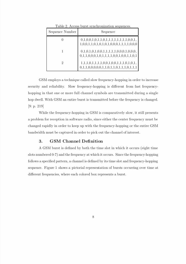
Table 2. Access burst synchronization sequences.
Sequence Number Sequence
0 0,1,0,0,1,0,1,1,0,1,1,1,1,1,1,1,1,0,0,1,
1,0,0,1,1,0,1,0,1,0,1,0,0,0,1,1,1,1,0,0,01 0,1,0,1,0,1,0,0,1,1,1,1,1,0,0,0,1,0,0,0,
0,1,1,0,0,0,1,0,1,1,1,1,0,0,1,0,0,1,1,0,1
2 1,1,1,0,1,1,1,1,0,0,1,0,0,1,1,1,0,1,0,1,0,1,1,0,0,0,0,0,1,1,0,1,1,0,1,1,1,0,1,1,1
GSM employs a technique called slow frequency-hopping in order to increase
security and reliability. Slow frequency-hopping is different from fast frequency-
hopping in that one or more full channel symbols are transmitted during a single
hop dwell. With GSM an entire burst is transmitted before the frequency is changed.
[9: p. 219]
While the frequency-hopping in GSM is comparatively slow, it still presents
a problem for reception in software radio, since either the center frequency must be
changed rapidly in order to keep up with the frequency-hopping or the entire GSM
bandwidth must be captured in order to pick out the channel of interest.
3. GSM Channel Definition
A GSM burst is defined by both the time slot in which it occurs (eight time
slots numbered 0-7) and the frequency at which it occurs. Since the frequency-hopping
follows a specified pattern, a channel is defined by its time slot and frequency-hopping
sequence. Figure 1 shows a pictorial representation of bursts occurring over time at
different frequencies, where each colored box represents a burst.
8
5/12/2018 GetTRDoc - slidepdf.com
http://slidepdf.com/reader/full/gettrdoc-55a35d023bc26 35/116
Figure 1. Illustration of a frequency-hopping GSM channel.
a. GSM Control Channels
The GSM specification distinguishes between traffic channels, which
carry voice and other data, and control channels which are used to gain access to the
traffic channels [10]. Also, the initial bursts that occur to gain access to control chan-
nels do not make use of frequency-hopping, simplifying the detection and decoding of
control traffic [11]. For this reason, this research focuses on the bursts that are used
to access a GSM network.
B. GSM MODULATION
The following section describes the physical layer modulation in the GSM sys-
tem. This does not include any discussion of higher level layer coding and interleaving,
both of which exist in GSM, but are beyond the scope of this thesis.
The GSM system uses differential encoding of data bits and GMSK as its
modulation scheme.
9
5/12/2018 GetTRDoc - slidepdf.com
http://slidepdf.com/reader/full/gettrdoc-55a35d023bc26 36/116
1. Differential Encoding
According to the GSM specification covering physical layer modulation, before
data bits are modulated, they are encoded using differential encoding as follows [12]:
di = di ⊕ di−1 where ⊕ denotes modulo 2 addition. (2.1)
The input to the differential encoder described in 2.1 is specified to consist of
a series of zeros and ones. However, the output of the differential encoder is ±1, so
the signal must be level-shifted as follows [12]:
αi = 1 − 2di (2.2)
The output of the differential encoder is αi, which is a differentially encoded
polar signal.
2. GMSK Filtering
The binary data to be modulated using GMSK can be represented as a series
of polar, differentially encoded impulses, as follows [12]:
∞i=0
αiδ(t− iT b) (2.3)
This set of impulses is convolved with a function g(t), the impulse response of
a Gaussian-shaped filter, to give the GMSK waveform [12]:
g(t) = h(t) ∗ rect
t
T b
(2.4)
where the function rect(x) is the rectangular function with an area of one and a width
of one bit duration [12] and is defined by
rect
t
T b
=
1
T bfor |t| <
T b2
(2.5)
rect
t
T b
= 0 otherwise (2.6)
10
5/12/2018 GetTRDoc - slidepdf.com
http://slidepdf.com/reader/full/gettrdoc-55a35d023bc26 37/116
T b in Equation (2.5) is the bit duration, which is 61625×103
seconds, or approxi-
mately 3.69 microseconds [12]. h(t) is a Gaussian impulse response:
h(t) =exp
−t2
2δ2T 2b √2πδT b(2.7)
where δ is defined to be inversely proportional to the bandwidth-time product [12]:
δ =
ln(2)
2πBT band BT b = 0.3 (2.8)
BT b (also called the bandwidth-time product) is the product of the the 3 dB band-
width of the filter and the bit duration and is a constant (0.3 in the case of GSM).
This affects the amount of inter-symbol interference in the GMSK signal. The 0.3
chosen for GSM is a compromise between error rate and spectral efficiency. [13: p.
319]
11
5/12/2018 GetTRDoc - slidepdf.com
http://slidepdf.com/reader/full/gettrdoc-55a35d023bc26 38/116
C. THE UNIVERSAL SOFTWARE RADIO PERIPHERAL
The Universal Software Radio Peripheral (USRP) is a hardware device that
makes reception and transmission of radio waves with consumer-grade, personal com-
puter equipment possible. It consists of a motherboard containing various ADCs,
digital-to-analog (DAC) converters, an FPGA, and slots for a number of daughter-
boards, which determine the range of frequencies the board can send or receive. The
USRP connects to the computer via a high-speed Universal Serial Bus (USB) port.
[14]
1. Receive Capabilities
a. Analog-to-digital Conversion
The frequency band of the analog signals coming into the USRP moth-erboard is determined by the specific daughter-board that is used with the USRP.
The daughter-board is responsible for providing the separated I and Q channels of the
complex signal to the motherboard and possibly for converting the received real signal
at RF to a complex signal at an intermediate frequency (IF). Some daughter-boards
perform no conversion, so as to be useful with a variety of low frequency signals.
The particular board used for this research, however, did perform conversion, so the
analysis of its operation follows. [14]The signal at the antenna of the daughter-board can be described as
the signal r(t), which has a carrier of frequency f RF modulated by amplitude A(t)
and phase θ(t):
r(t) = A(t)cos(2πf RF + θ(t)) (2.9)
12
5/12/2018 GetTRDoc - slidepdf.com
http://slidepdf.com/reader/full/gettrdoc-55a35d023bc26 39/116
After the daughter-board performs frequency conversion and filtering
to remove unwanted aliasing, the resulting complex signal analytic signal, S (t) =
S i(t) + jS q(t), can be described by
S i(t) = A(t)cos(2πf IF + θ(t)) (2.10)
S q(t) = A(t)sin(2πf IF + θ(t)) (2.11)
The preceding signals are then sampled by the ADCs after an optional
amplification stage using a Programmable Gain Amplifier (PGA) on the USRP moth-
erboard, which provides a gain of up to 20 dB. The USRP contains four 12-bit ADCs
(each is dedicated to the I or Q samples of one of two possible channels) each running
at 64×106
samples/s, giving a theoretical upper frequency limit (for the intermediatefrequency) of 32 MHz before artifacts due to aliasing are introduced. Note that two
separate ADCs are required to convert the complex signal to a digital representation.
The resulting sampled data is
S i[n] = S i(nT s) (2.12)
S q[n] = S q(nT s) (2.13)
where T s is the sample interval, n = 0, 1, 2,... is discrete time, and S i[n] and S q[n] are
the resulting in-phase and quadrature samples, respectively. [14]
13
5/12/2018 GetTRDoc - slidepdf.com
http://slidepdf.com/reader/full/gettrdoc-55a35d023bc26 40/116
b. Conversion to Baseband
After translation into the digital domain, the samples are processed by
firmware on the FPGA. Each pair of incoming I and Q samples are treated as a single
complex analytic sample S i[n] + jS q[n] by the multiplication algorithm in the FPGAwhich performs a complex multiplication resulting in a set of complex samples at
baseband I [n] + jQ[n] and given by [14]
S [n] = S i[n] + jS q[n] (Complex Analytic Signal)
= A(nT s) [cos(2πf IF nT s + θ(nT S )) + j sin(2πf IF (nT s) + θ(nT s))]
= A(nT s)e j2πf IF (nT s)+θ(nT s) (2.14)
I [n] + jQ[n] = S [n]e− j2πf IF (nT s)
= A(nT s)eθ(nT s) (Complex Envelope) (2.15)
I [n] and Q[n] are the outputs of the first stage of the FPGA. Low-pass
filtering is accomplished in the next stage in addition to decimation [14]. Decimation
reduces the effective sample rate and, therefore, the signal bandwidth. Filtering is
required because decimation itself will introduce aliasing if the decimation rate is
large enough[15: p. 235].
c. Aliasing
Aliasing occurs because frequencies which differ by a multiple of the
sampling rate are indistinguishable from each other after sampling [15: p. 11]. To
illustrate this mathematically, the angular frequency Ω0 and the angular digital fre-
quency ω0 are defined as:
Ω0 = 2πF 0 =2π
T 0(2.16)
ω0 = Ω0T s = 2πF 0F s
radians (2.17)
14
5/12/2018 GetTRDoc - slidepdf.com
http://slidepdf.com/reader/full/gettrdoc-55a35d023bc26 41/116
where F 0 is the frequency of interest of the continuous time signal and F s is the
sampling frequency. The digital frequency is shown to be dependent on the sampling
frequency, which is an important distinction. Because decimation effectively lowers
the sampling frequency F s, the digital frequency that corresponds to a frequency F
0
changes proportionally. [15]
One other important property of digital frequency is that any frequency
ω1 and another frequency ω2 are indistinguishable from each other in the discrete
domain provided that ω2 = ω1 + k2π, where k is any integer. This is why frequencies
above the Nyquist rate are indistinguishable from frequencies below it and is the basis
for understanding aliasing. Notice that the Nyquist frequency, which is defined as
one-half the sample rate, corresponds to an angular digital frequency of π. Therefore,
a discrete time signal’s bandwidth must exist entirely between −π and π in order for
aliasing not to occur. [15]
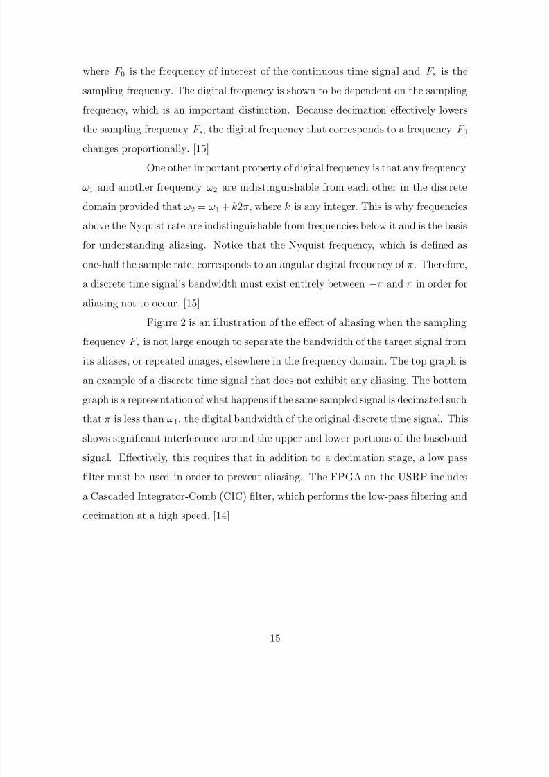
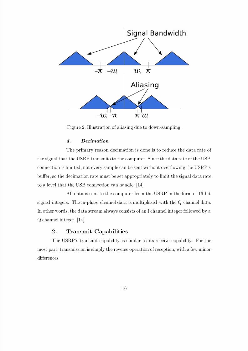
Figure 2 is an illustration of the effect of aliasing when the sampling
frequency F s is not large enough to separate the bandwidth of the target signal from
its aliases, or repeated images, elsewhere in the frequency domain. The top graph is
an example of a discrete time signal that does not exhibit any aliasing. The bottom
graph is a representation of what happens if the same sampled signal is decimated such
that π is less than ω1, the digital bandwidth of the original discrete time signal. This
shows significant interference around the upper and lower portions of the baseband
signal. Effectively, this requires that in addition to a decimation stage, a low pass
filter must be used in order to prevent aliasing. The FPGA on the USRP includes
a Cascaded Integrator-Comb (CIC) filter, which performs the low-pass filtering and
decimation at a high speed. [14]
15
5/12/2018 GetTRDoc - slidepdf.com
http://slidepdf.com/reader/full/gettrdoc-55a35d023bc26 42/116
Figure 2. Illustration of aliasing due to down-sampling.
d. Decimation
The primary reason decimation is done is to reduce the data rate of
the signal that the USRP transmits to the computer. Since the data rate of the USB
connection is limited, not every sample can be sent without overflowing the USRP’s
buffer, so the decimation rate must be set appropriately to limit the signal data rate
to a level that the USB connection can handle. [14]
All data is sent to the computer from the USRP in the form of 16-bit
signed integers. The in-phase channel data is multiplexed with the Q channel data.
In other words, the data stream always consists of an I channel integer followed by a
Q channel integer. [14]
2. Transmit Capabilities
The USRP’s transmit capability is similar to its receive capability. For the
most part, transmission is simply the reverse operation of reception, with a few minor
differences.
16
5/12/2018 GetTRDoc - slidepdf.com
http://slidepdf.com/reader/full/gettrdoc-55a35d023bc26 43/116
The data to be transmitted is sent to the USRP over the USB connection.
This data is then interpolated at a specified rate, which may be set programatically.
Interpolation, like decimation, introduces aliasing into the signal, so the signal must
be filtered afterward [15: p. 248]. Next, the signal is multiplied by a sinusoid at the
intermediate frequency, converted to analog by the digital-to-analog converter (DAC)
at a rate of 128× 106 samples/s, with the resulting signal sent to the daughter-board
for transmission [14]. The 128× 106 sample/second DAC rate gives us a maximum
intermediate frequency of 64MHz [14]. However, the maximum allowable intermediate
frequency is limited to 44 MHz by the USRP software to make up-sampling and
filtering practical [14, 16].
According to the USRP documentation, the required sample rate sent over the
USB connection is
RUS B =F DAC
Rinterp
× channels (2.18)
where F DAC is the sample frequency of the DAC, Rinterp is the interpolation rate, and
channels is the number of simultaneous data signals being transmitted [16]. This
sample rate is measured in terms of individual 16-bit integers being sent over the
USB wire. This rate is important when generating the baseband signal, both in
determining the rate at which to sample the ideal baseband signal and in providingthe maximum rate across the USB connection to create a more accurate output signal.
3. Data Transfer Capabilities
The theoretical maximum transfer rate of the USB 2.0 connection that the
USRP uses to transfer data is 480 Mbit/sec, but in practice the maximum is found to
be about 32 MB/sec, or 256Mbit/sec [14]. Each complex sample consists of a 16-bit
17
5/12/2018 GetTRDoc - slidepdf.com
http://slidepdf.com/reader/full/gettrdoc-55a35d023bc26 44/116
signed integer for the I and the Q channels, totaling 32 bits per complex sample [14].
Therefore, the maximum sample rate coming in to (or going out of) the computer’s
USB port is
Rs = 256× 106 bits
s ×1
32
sample
bits = 8 × 10⁶samples
s (2.19)
This allows the calculation of the minimum sample interval
T s =1
8 × 10⁶s
samples= 125 ns (2.20)
This minimum sample interval is used later to calculate the precision of performing
geolocation using digital samples.
D. SIGNAL DETECTION
1. Correlator
Determining that the signal of interest has been received is a matter of correlat-
ing the incoming signal with the known training sequence that has been modulated
with GMSK. The sampling frequency associated with this known sequence should
match the sampling frequency of the data coming in over the USB link.
Let the signal of interest be sampled signal X and the incoming sampled signal
be signal Y . From the USRP, X will be a multiplexed complex signal with 16-bit I
and Q samples, respectively. In hardware, we normally perform separate convolutions
on the I and Q channels and sum the result [17: p. 232]. Theoretically this is
not necessary in software, however, since we can construct an identical multiplexed
complex signal and correlate against that. Unfortunately, test results show that
other factors prevent this straightforward approach from working easily and will be
discussed in Chapter IV.
Correlation consists of performing a non-time-reversed convolution between X
and Y . In the discrete domain, we may define the correlation at a certain time t as
follows, assuming the input X is the same length as the target signal Y
C =n−1i=0
X iY i (2.21)
18
5/12/2018 GetTRDoc - slidepdf.com
http://slidepdf.com/reader/full/gettrdoc-55a35d023bc26 45/116
where n is the number of samples contained in the signal of interest. If the signals X
and Y match exactly, the magnitude of C is large and a spike occurs in the graph of
C over time.
However, since we are receiving the signal continuously, Y does not simply
consist of only n samples but may be arbitrarily long. Because of this, we must keep
shifting the samples in Y by one, such that Y 1 becomes the new Y 0, Y 2 becomes the
new Y 1, and so forth. The output of the correlator at each iteration is checked to see
if its value is above a threshold, at which point we can be reasonably certain that the
target signal has been received. Additionally, the maximum value of the correlator
output that is above the threshold allows us to determine the exact time that the
signal was received to the nearest sampling interval. [17]
E. GEOLOCATION
Location of an emitter in this system is done by measuring the time differ-
ence of arrival between identical listening posts. This requires at least two posts to
calculate the distance from either post and at least three to perform an accurate
triangulation. [2]
1. RequirementsIn the case of only two listening posts on either side of an emitter, the emitter
can be located on a hyperbolic curve between the two posts. The hyperbolic curve is a
representation of all points where the signed difference of the distance between either
post (focus) and the emitter is a constant. This constant is equal to the distance
traveled by light between the time the signal is first detected (at one post) and the
time it is detected at the second post.[2: p. 174]
Using only two posts, an accurate measurement of distance can be made, butthe emitter can still only be said to be located anywhere on a hyperbolic curve that
is infinitely long.
19
5/12/2018 GetTRDoc - slidepdf.com
http://slidepdf.com/reader/full/gettrdoc-55a35d023bc26 46/116
By using another listening post, two more such curves can be found. Ideally,
the intersection of these curves occurs at the exact location of the emitter. Accuracy
and precision can be increased by using more receivers. Since any single curve is
dependent on the time difference between exactly two receivers, the number of unique
curves N that can be plotted based on the number of listening posts L is
N =L(L− 1)
2(2.22)
2. Precision
Because the USB 2.0 link is the bottleneck for data transfer into the computer
and the precision of the geolocation directly depends on the sample interval, the
maximum precision can be calculated. From Equation (2.20), the minimum sample
interval is 125 nanoseconds. In that time, an RF signal will travel a distance
Ds = T sc = (125× 10−9)s × (3 × 108)m
s= 37.5 m (2.23)
3. Limitations and Workarounds
Although four listening posts provide six curves and improved accuracy, calcu-
lation of the points on each curve and the intersection of those points, particularly in
the presence of measurement error, is computationally intensive. Additionally, even
the slightest measurement error means that the hyperbolic curves have no simulta-
neous solution or point where every curve intersects. Also, the nature of hyperbolic
equations imparts a floating-point inaccuracy to computer calculations dependent
on which part of the curve the emitter is actually located. Finally, calculation of a
hyperbolic curve involves trigonometric functions which are not practical for heavy
real-time usage, even with modern hardware. Therefore, another approach is needed.
a. Graphical Method
The most obvious method is to use graphical analysis to show the likely
position of the emitter. To illustrate this method, we assume there exist four listening
posts located in a square configuration on a Cartesian coordinate system at points
20
5/12/2018 GetTRDoc - slidepdf.com
http://slidepdf.com/reader/full/gettrdoc-55a35d023bc26 47/116
(0,0), (0,1000), (1000,0), and (1000,1000). This creates a 1000 × 1000 grid between
the posts. This grid can be superimposed on any two dimensional surface with grid
coordinates translated to map coordinates, latitudes and longitudes, etc.
The emitter can be found by calculating the likelihood of it being lo-
cated at any coordinate on the grid based on the time differences of arrival between
the listening posts. Since the output of the algorithm is a two-dimensional matrix of
probabilities, the output is easily represented as a computer graphic. This method is
used to simulate finding the location of the emitter in Chapter IV.
b. Lookup Table Method
The complexity and run-time of the location calculation can be reduced
even further. Ideally, the result of the calculation is a coordinate on the computedgrid based on a series of time-differences-of-arrival. Note that each point P on the
grid ideally maps to a unique set of time-differences between three listening posts:
P ij maps to [τ 01, τ 02, τ 12] (2.24)
where τ ab is the time-difference-of-arrival between two listening posts a and b. There-
fore, the calculation of the ideal time differences of each point on the grid can be
done prior to the deployment of the system. Then the identification of the mostlikely location of an emitter can be reduced to a table lookup/interpolation of the
time differences, which could happen in real time. The only limitation is the stor-
age space required to hold such a table and the fact that movement of the receivers
requires a table update. As such, the lookup table approach is not practical for a
system in which the receivers are mobile.
21

5/12/2018 GetTRDoc - slidepdf.com
http://slidepdf.com/reader/full/gettrdoc-55a35d023bc26 48/116
F. CONCLUSION
We have examined the mathematical theory behind generation, transmission,
reception, and detection of the time of arrival of a GSM access burst in this chapter.
Also discussed were the theoretical limitations of the accuracy and precision of a
software radio. What remains is the translation of that theory into actual algorithms
that can be used in software. The translation is challenging because continuous time
signals are generated in discrete time for transmission. The following chapter focuses
on overcoming those challenges.
22
5/12/2018 GetTRDoc - slidepdf.com
http://slidepdf.com/reader/full/gettrdoc-55a35d023bc26 49/116
III. IMPLEMENTATION
A. GMSK SIGNAL GENERATION
1. GMSK Filter Implementation
The GMSK definition in Chapter II must be used to generate a GMSK signal.
However, the GMSK signal is defined in the continuous time domain and must be
converted to the discrete domain before it can be used. There are two rates to be
concerned with when performing this conversion: the GMSK bit rate, Rb = 1/T b; and
the sampling rate that is used to convert the continuous GMSK signal to the discrete
domain.
Equation (2.1) through Equation (2.8) suggest that a series of impulses repre-
senting the data bits should be convolved with the defined impulse response function,
which itself contains a convolution:
x(t) =
∞i=0
αiδ(t − iT b) ∗
h(t) ∗ rect
t
T b
(3.1)
where ∗ implies convolution. The result x(t) is the signal which subsequently fre-
quency modulates the signal carrier. Because convolution is an associative and com-
mutative operation [18], we can rewrite the process as
x(t) =
∞
i=0
αiδ(t − iT b) ∗ rect
t
T b
∗ h(t) (3.2)
= b(t) ∗ h(t) (3.3)
Instead of performing two convolutions on the continuous data and then sam-
pling that, we can simply perform a discrete convolution on a discrete function h[k]
and a discrete series of rectangular pulses b[k]. The functions h[k] and b[k] are equal
to the sampled continuous h(t) and b(t), respectively, and are given by
h[k] = h(nT s) (3.4)
b[k] = b(nT s) (3.5)
23
5/12/2018 GetTRDoc - slidepdf.com
http://slidepdf.com/reader/full/gettrdoc-55a35d023bc26 50/116
where T s is equal to some sample time. The rectangular pulses in b[k] represent
the data-bearing impulses already convolved with the discrete rect[x] function and,
therefore, look like
(1, 1, 1, 1, 1,−1,−1,−1,−1,−1,...) if αi = [1, −1, ...] (3.6)
The above is equivalent to sampling the input data b(t) at some rate Rs = n/T b,
where n = 5, and the time difference between the successive bits 1 and −1 is T b. In
other words, each sample represents T b/n seconds. The result is achieved simply by
repeating the input data bits n times, which saves significant computation time and
is less complex to implement than performing multiple convolutions.
2. Determining the Sample Rate
Before generating a discrete-time GMSK signal, the appropriate sample rate
must be determined. The required sample rate for transmission is determined solely
by the configuration of the USRP, which expects samples at a rate dependent on the
number of channels used, the frequency of the DAC, and the interpolation rate.
The DAC frequency on the USRP is constant at a rate of 128 × 106 complex
samples/s. The GMSK generation function generates pairs of 16-bit integers where
each pair represents one complex sample. The only variable is the interpolation rate.
This is a design decision. A lower interpolation rate results in a more accurate signal,
while a higher one requires less bandwidth from the USB link. Since the USRP in
our case is dedicated to transmitting a signal, we can use all of the USB bandwidth
if necessary.
Equation (2.19) shows that the maximum USB bandwidth is 8 × 10⁶ complex
samples/s. Substituting this into Equation (2.18), along with the constants already
mentioned, we get an interpolation rate of 32, which is the lowest acceptable inter-
polation rate that does not saturate the USB connection.
24
5/12/2018 GetTRDoc - slidepdf.com
http://slidepdf.com/reader/full/gettrdoc-55a35d023bc26 51/116
Since signal accuracy is important for this experiment, the minimum interpo-
lation rate of 32 is used. Thus, the complex sample rate can be calculated, (keeping in
mind that a complex sample consists of two 16-bit samples for the I and Q channels):
Rstx = 128 × 106
32= 4× 10⁶ samples
s(3.7)
T stx =1
Rstx
= 2.5 × 10⁻⁷s (3.8)
Rstx is the minimum required sample rate for our discrete generated signal. Note that
any integer multiple nRstx works equally well – we simply have to select every nth
sample to send to the USRP. However, there is another rate to consider, and that is
the GMSK bit rate of Rb = 1625 × 103/6 (bits/second) [12]. We have seen that it
is very convenient if the sample rate used is some integer multiple of the GMSK bit
rate. So we now have two different rates that we would like to have as factors of the
overall sample rate, and we need to find integers n0 and n1 such that:
n0Rstx = n1Rb (3.9)
n0
n1
=Rb
Rstx
=1625 × 103
6(4× 10⁶)=
13
96(3.10)
The overall sample rate Rs that we would like to use is 13(4×10⁶) or 192(1625×103/6),
both of which are equal to 52 × 106. This ensures that no interpolation has to be
done when calculating samples for either the GMSK bit rate or the USB sample rate.
3. Baseband Signal Generation
To understand how the baseband signal is generated, a review of the source
code is helpful. The Common Lisp code generates a complex baseband frequency
modulated signal, one sample at a time. It keeps track of the phase angle of the lastsample using the phase-angle variable. The reset function is called to set the phase
angle to zero. The signal is generated by calling the modfm function repeatedly, with
the interval between the samples and the instantaneous frequency as arguments.
25
5/12/2018 GetTRDoc - slidepdf.com
http://slidepdf.com/reader/full/gettrdoc-55a35d023bc26 52/116
The modfm function calculates the new phase angle based on the old phase
angle and the phase change that is calculated based on the new frequency and the
sample interval. A complex number is returned that represents the complex amplitude
of the current sample. The preceding is accomplished by the code:
;;; fm signal
(let ((phase-angle 0))
(defun reset ()
(setf phase-angle 0))
(defun modfm (sample-duration freq)
(let ((phase-inc (* 360 sample-duration freq))) ;;in degrees
(setf phase-angle (+ phase-angle phase-inc))(exp (* j (radian phase-angle))))))
The preceding code implements the mathematical function
modfm(θ p, T stx , F ∆) = e j(θp+(T stx×F ∆)) (3.11)
where θ p is the phase angle calculated from the previous sample, T stx is the sample
duration, and F ∆ is the instantaneous frequency to be encoded. The result is a
complex vector which can be separated into I and Q samples for transmission.
This function, in combination with another function that performs a linear
translation of voltage to frequency, is called a numerically controlled oscillator (NCO).
It takes a normalized input voltage and produces a complex baseband FM signal as
its output. One of the most desirable features of an NCO is that it generates a signal
that is as close to mathematically perfect as possible and the output does not vary
with temperature or other factors that affect an analog voltage controlled oscillator.
This is why it is practical to generate the GMSK signal with a simple algorithm
instead of modeling the more complex analog circuits in software [1].
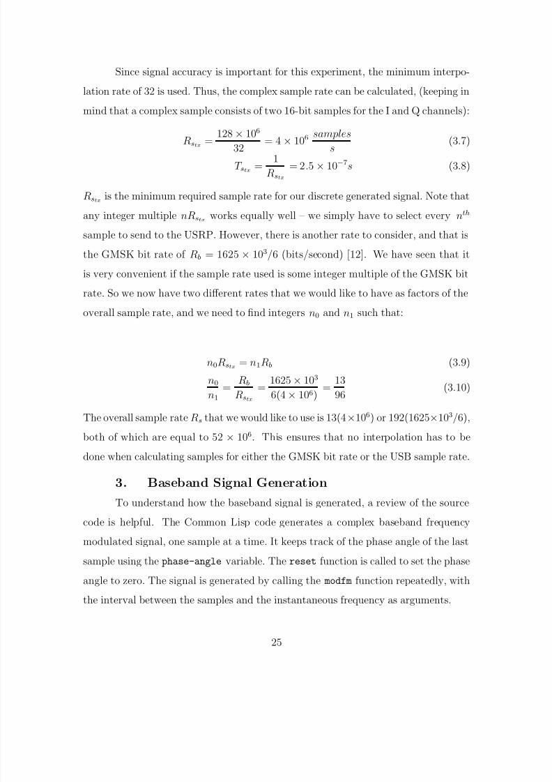
Figure 3 shows an example of the output of this NCO algorithm where the
instantaneous frequency starts at −10 Hz and slowly increases to 10 Hz.
26
5/12/2018 GetTRDoc - slidepdf.com
http://slidepdf.com/reader/full/gettrdoc-55a35d023bc26 53/116
-1
-0.5
0
0.5
1
1.5
0 500 1000 1500 2000
A m p l i t u d e
Samples
IQ
Figure 3. Complex FM baseband signal from −10 to 10 Hz.
4. Application of a GMSK Filter
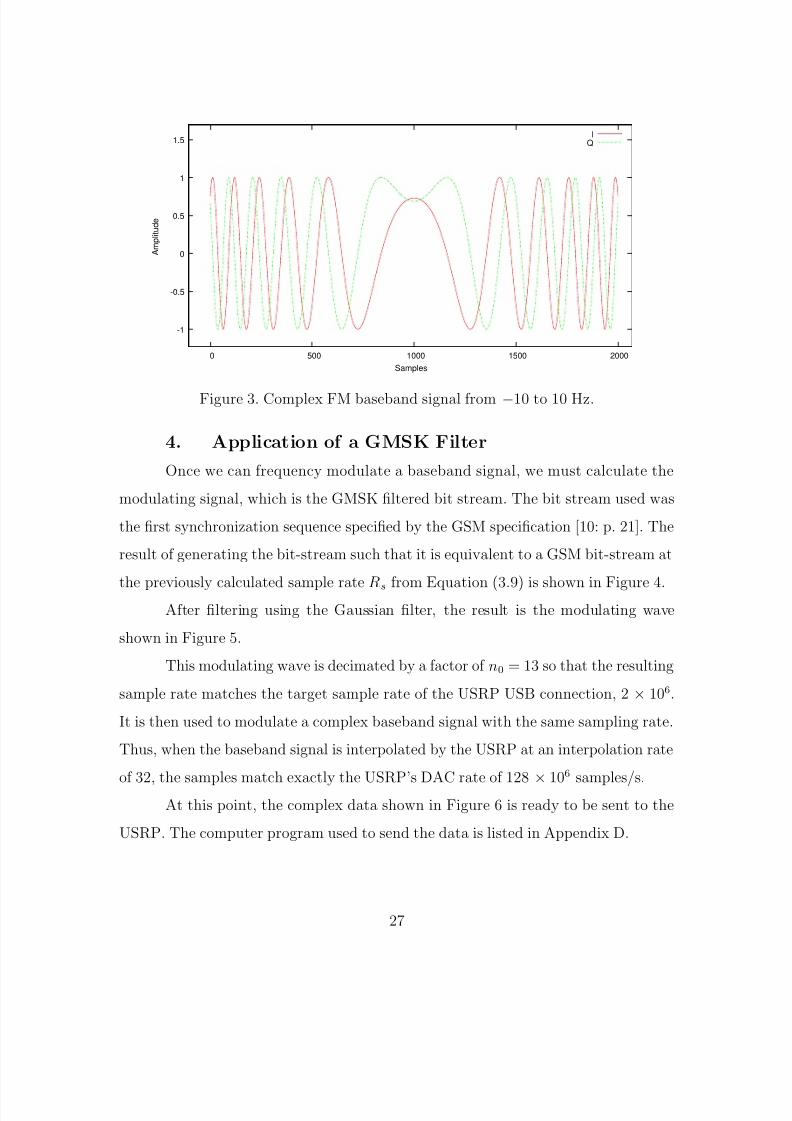
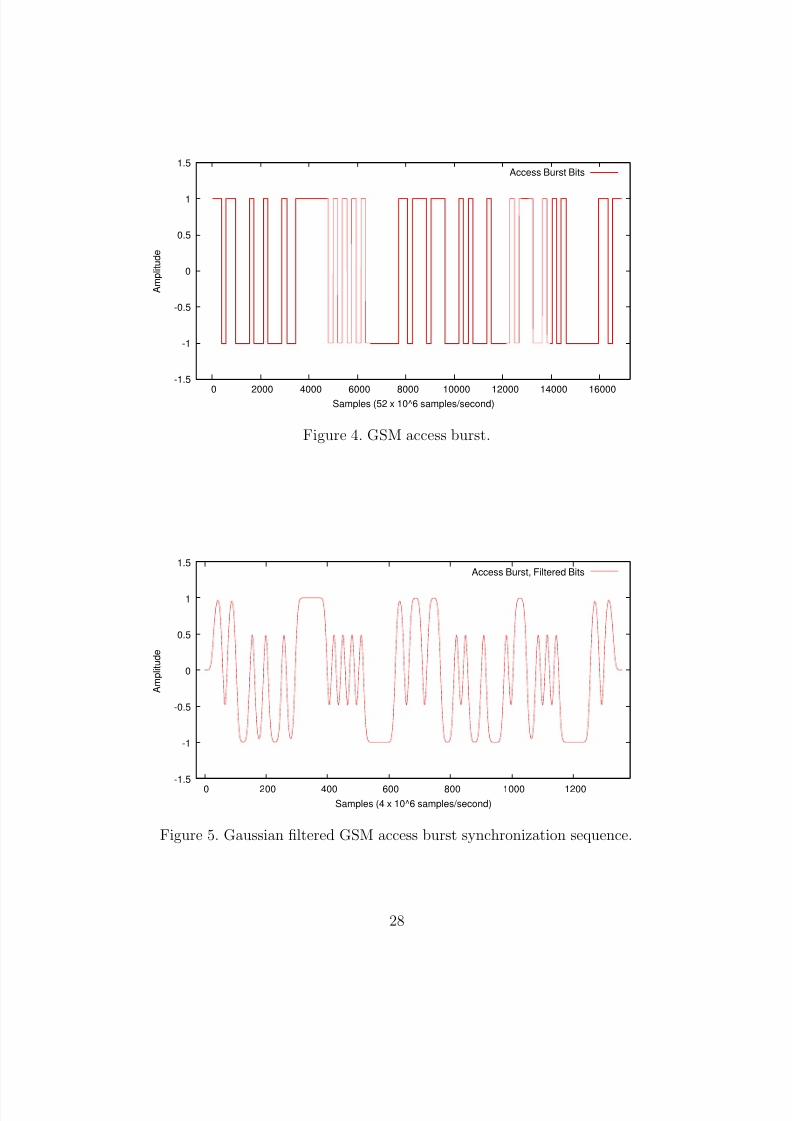
Once we can frequency modulate a baseband signal, we must calculate the
modulating signal, which is the GMSK filtered bit stream. The bit stream used was
the first synchronization sequence specified by the GSM specification [10: p. 21]. The
result of generating the bit-stream such that it is equivalent to a GSM bit-stream at
the previously calculated sample rate Rs from Equation (3.9) is shown in Figure 4.After filtering using the Gaussian filter, the result is the modulating wave
shown in Figure 5.
This modulating wave is decimated by a factor of n0 = 13 so that the resulting
sample rate matches the target sample rate of the USRP USB connection, 2 × 10⁶.
It is then used to modulate a complex baseband signal with the same sampling rate.
Thus, when the baseband signal is interpolated by the USRP at an interpolation rate
of 32, the samples match exactly the USRP’s DAC rate of 128 × 106
samples/s.At this point, the complex data shown in Figure 6 is ready to be sent to the
USRP. The computer program used to send the data is listed in Appendix D.
27
5/12/2018 GetTRDoc - slidepdf.com
http://slidepdf.com/reader/full/gettrdoc-55a35d023bc26 54/116
-1.5
-1
-0.5
0
0.5
1
1.5
0 2000 4000 6000 8000 10000 12000 14000 16000
A m p l i t u d e
Samples (52 x 10^6 samples/second)
Access Burst Bits
Figure 4. GSM access burst.
-1.5
-1
-0.5
0
0.5
1
1.5
0 200 400 600 800 1000 1200
A m p l i t u d e
Samples (4 x 10^6 samples/second)
Access Burst, Filtered Bits
Figure 5. Gaussian filtered GSM access burst synchronization sequence.
28
5/12/2018 GetTRDoc - slidepdf.com
http://slidepdf.com/reader/full/gettrdoc-55a35d023bc26 55/116
-30000
-20000
-10000
0
10000
20000
30000
2600 2800 3000 3200 3400 3600 3800 4000 4200
A m p l i t u d e
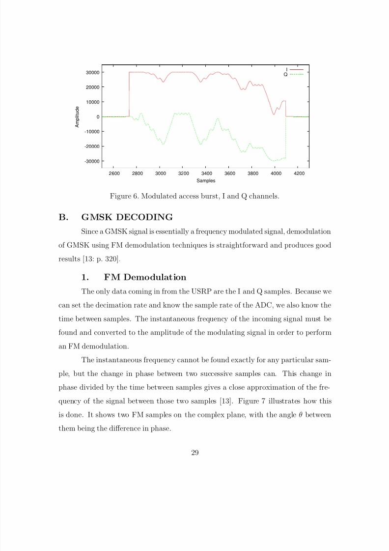
Samples
IQ
Figure 6. Modulated access burst, I and Q channels.
B. GMSK DECODING
Since a GMSK signal is essentially a frequency modulated signal, demodulation
of GMSK using FM demodulation techniques is straightforward and produces good
results [13: p. 320].
1. FM Demodulation
The only data coming in from the USRP are the I and Q samples. Because we
can set the decimation rate and know the sample rate of the ADC, we also know the
time between samples. The instantaneous frequency of the incoming signal must be
found and converted to the amplitude of the modulating signal in order to perform
an FM demodulation.
The instantaneous frequency cannot be found exactly for any particular sam-
ple, but the change in phase between two successive samples can. This change in
phase divided by the time between samples gives a close approximation of the fre-
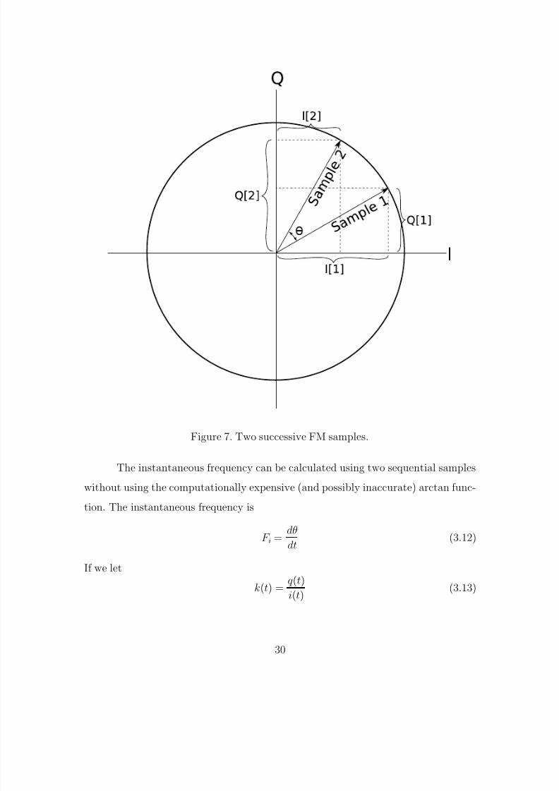
quency of the signal between those two samples [13]. Figure 7 illustrates how this
is done. It shows two FM samples on the complex plane, with the angle θ between
them being the difference in phase.
29
5/12/2018 GetTRDoc - slidepdf.com
http://slidepdf.com/reader/full/gettrdoc-55a35d023bc26 56/116
Figure 7. Two successive FM samples.
The instantaneous frequency can be calculated using two sequential samples
without using the computationally expensive (and possibly inaccurate) arctan func-
tion. The instantaneous frequency is
F i =dθ
dt(3.12)
If we let
k(t) =q(t)
i(t)(3.13)
30
5/12/2018 GetTRDoc - slidepdf.com
http://slidepdf.com/reader/full/gettrdoc-55a35d023bc26 57/116
and
θ(t) = arctan (k(t)) (3.14)
then taking the derivative of Equation (3.13), we get
dk
dt=
i dqdt − q di
dt
i2(3.15)
Computing the derivative of Equation (3.14), we get
dθ
dt=
1
1 + (k)2dk
dt
=1
1 +
q
i
2
i dq
dt− q di
dt
i2
=i dq
dt −q di
dti2 + q2 (3.16)
which is equal to the instantaneous frequency. In the discrete domain, di/dt and
dq/dt can be calculated by dividing (q[x] − q[x − 1]) and (i[x] − i[x − 1]) each by
the sample duration. The results here are consistent with the result of the discussion
found in [19].
2. Determining Sample Rate
Ideally, we want to be able to use the lowest possible decimation rate when
receiving to get the most accurate results possible. According to Equation (2.19),
the maximum sample rate the USB connection can handle is 8× 10⁶ samples/s. This
corresponds to a decimation rate of eight, since the ADCs in the USRP operate at a
rate of 64 × 106 samples/s, as shown by
RUS B =RADC
Rdecim
(3.17)
where
Rdecim =64× 106
8 × 106= 8 (3.18)
where RU SB is the data rate limit of the USB connection, and RADC is the rate of
the USRP’s ADC.
31
5/12/2018 GetTRDoc - slidepdf.com
http://slidepdf.com/reader/full/gettrdoc-55a35d023bc26 58/116
However, initial testing showed that over longer data collection runs, the rate
at which the data could be transferred to the hard disk from memory became a
limiting factor. Since a single buffer overrun means that samples are lost and the
time of arrival calculation is incorrect, the decimation rate must be set high enough
to ensure all data can be copied to the hard disk for the entire collection without any
overruns. Testing indicated that a decimation rate of 16 produced a rare overrun,
and a decimation rate of 32 was high enough so that no overruns occurred. For
the purposes of the following illustration of the demodulation process, however, a
decimation rate of 16 was used as it was the best compromise between performance
and precision.
A decimation rate of 16 gives the incoming sample rate for the received signal:
RsRx=
64 × 106
Rdecim
=64 × 106
16= 4 × 10⁶
samples
s(3.19)
3. Generating Target Sequence
In order to detect the GSM training sequence, we need to generate that se-
quence at the RsRxsample rate. This was done exactly the same way as for the
transmission signal by generating a baseband FM signal as in section (A.4). The
difference here is that the further steps of modulating a carrier signal were not taken,
since our received signal is frequency demodulated prior to correlation. The results
of this calculation are, therefore, the same as those of the intermediate step in the
generation of the transmission signal, shown in Figure 5.
4. Correlation
In order to perform the correlation, the incoming signal samples must be mul-
tiplied by the target signal samples. An array of the target samples is created in
order to perform the multiplication and summation as in Equation (2.21). The target
sequence is simply the training sequence portion of the access burst shown in Figure
5. These target samples are placed in the array in non-reversed time order such that
32
5/12/2018 GetTRDoc - slidepdf.com
http://slidepdf.com/reader/full/gettrdoc-55a35d023bc26 59/116
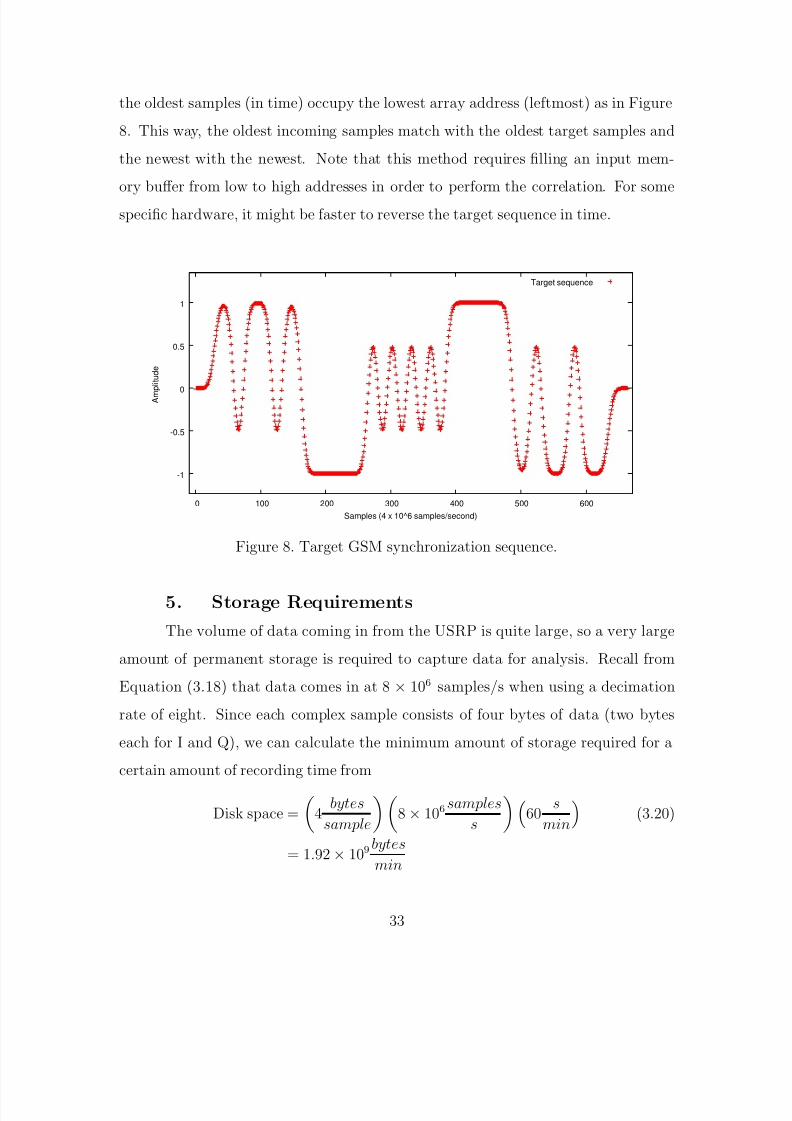
the oldest samples (in time) occupy the lowest array address (leftmost) as in Figure
8. This way, the oldest incoming samples match with the oldest target samples and
the newest with the newest. Note that this method requires filling an input mem-
ory buffer from low to high addresses in order to perform the correlation. For some
specific hardware, it might be faster to reverse the target sequence in time.
-1
-0.5
0
0.5
1
0 100 200 300 400 500 600
A m p l i t u d e
Samples (4 x 10^6 samples/second)
Target sequence
Figure 8. Target GSM synchronization sequence.
5. Storage Requirements
The volume of data coming in from the USRP is quite large, so a very large
amount of permanent storage is required to capture data for analysis. Recall from
Equation (3.18) that data comes in at 8 × 10⁶ samples/s when using a decimation
rate of eight. Since each complex sample consists of four bytes of data (two bytes
each for I and Q), we can calculate the minimum amount of storage required for a
certain amount of recording time from
Disk space =
4
bytes
sample
8 × 10⁶
samples
s
60
s
min
(3.20)
= 1.92× 109bytes
min
33
5/12/2018 GetTRDoc - slidepdf.com
http://slidepdf.com/reader/full/gettrdoc-55a35d023bc26 60/116
Equation (3.20) shows that with a decimation rate of eight, a minute of record-
ing takes up nearly two gigabytes of hard disk space. With the typical size of com-
modity hard drives today being 80-100 gigabytes, it would take under an hour to
completely fill the disk. Obviously, doubling the decimation rate would halve this re-
quirement, at the expense of geolocation precision. However, subsequent processing
of the data might increase the amount of storage needed. This is the case with the
GNU Radio tools, which store each complex sample as a pair of four byte floating
point values for a total of eight bytes per complex sample.
The storage requirements make it necessary to either do real-time or near-real
time processing of the data or to offload the data regularly to make room for new
collection.
C. CONCLUSION
This chapter discussed all of the implementation details that are necessary for
constructing a software radio based on the mathematical theory discussed in Chapter
II. What follows are the results of putting this implementation to the test, using two
computers each connected to a separate USRP, one to perform the signal generation
and transmission, and the other to receive the signal and perform the partial demod-
ulation and detection of the time-of-arrival. The following chapter also includes an
analysis of the actual accuracy and precision of the system as a whole.
34
5/12/2018 GetTRDoc - slidepdf.com
http://slidepdf.com/reader/full/gettrdoc-55a35d023bc26 61/116
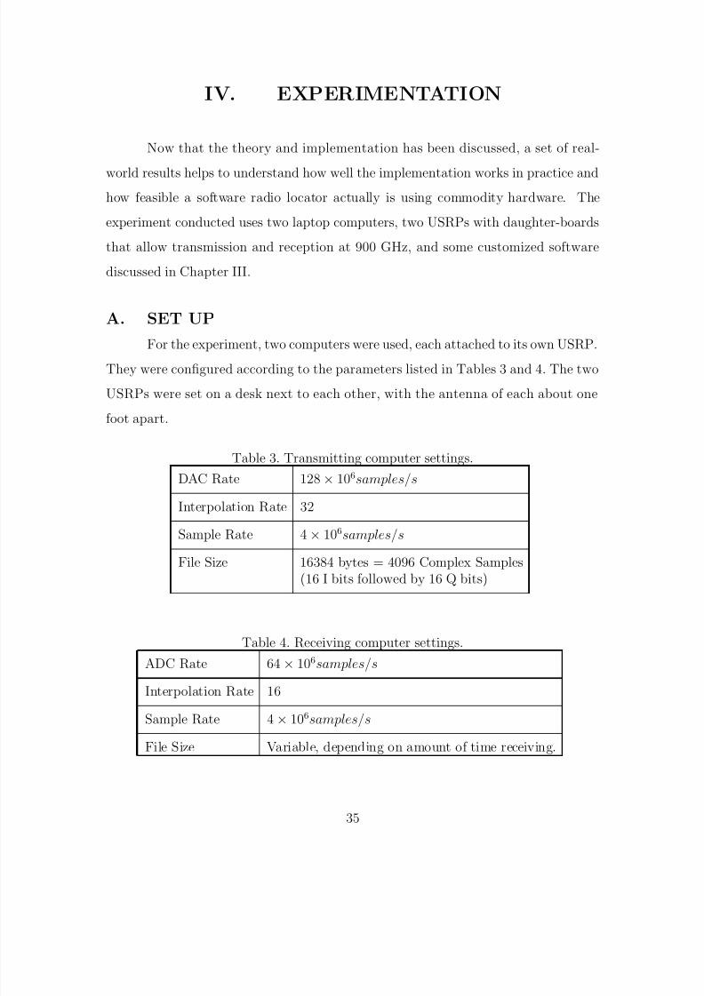
IV. EXPERIMENTATION
Now that the theory and implementation has been discussed, a set of real-
world results helps to understand how well the implementation works in practice and
how feasible a software radio locator actually is using commodity hardware. The
experiment conducted uses two laptop computers, two USRPs with daughter-boards
that allow transmission and reception at 900 GHz, and some customized software
discussed in Chapter III.
A. SET UP
For the experiment, two computers were used, each attached to its own USRP.They were configured according to the parameters listed in Tables 3 and 4. The two
USRPs were set on a desk next to each other, with the antenna of each about one
foot apart.
Table 3. Transmitting computer settings.
DAC Rate 128× 106samples/s
Interpolation Rate 32
Sample Rate 4 × 10⁶samples/s
File Size 16384 bytes = 4096 Complex Samples(16 I bits followed by 16 Q bits)
Table 4. Receiving computer settings.
ADC Rate 64 × 106samples/s
Interpolation Rate 16Sample Rate 4 × 10⁶samples/s
File Size Variable, depending on amount of time receiving.
35
5/12/2018 GetTRDoc - slidepdf.com
http://slidepdf.com/reader/full/gettrdoc-55a35d023bc26 62/116
B. TRANSMISSION
The transmitted signal samples for the GSM access burst were calculated in
accordance with the procedure outlined in previous chapters and stored in a 16384
byte file. This file size allows for 4096 complex samples. Since the burst itself only
takes 665 samples, the file was padded with samples of zero amplitude so that trans-
mission essentially pauses for a 3431-sample time period when not sending the access
burst. A small program was written with the GNU Radio software to send the con-
tents of the file repeatedly until the operator hit the Enter key on the keyboard. In
effect, the same access burst signal was sent repeatedly, every 4096 samples.
C. RECEPTION
For reception, the GNU Radio software was used to read the multiplexed I
and Q samples from the USRP and immediately write them to a file. No further
processing was done to the samples at this stage.
After the reception was complete, demodulation was performed on the raw I
and Q samples by a separate program, listed in Appendix G. It should be noted that
the demodulation was not done in real time. The GNU Radio software does have the
capability to demodulate FM signals in real time. This was tested and does indeed
work. However, as discussed below, additional flexibility in the FM demodulation
was needed, so a separate program was used instead.
1. Initial Results
The first FM demodulation, shown in Figure 9, shows a significant amount of
power when no signal is being transmitted. In fact, the noise is significantly more
powerful than the signal after being FM demodulated. This is to be expected, since
the white noise has large random variations in instantaneous frequency, but thisproblem had to be solved.
36
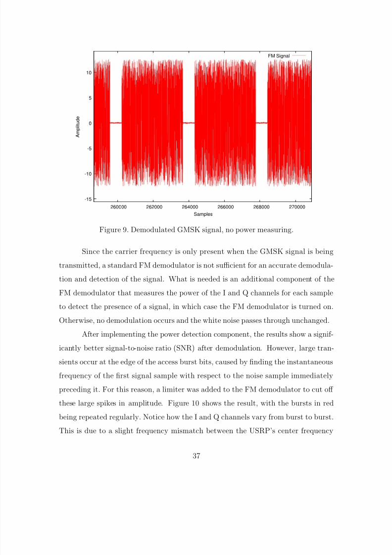
5/12/2018 GetTRDoc - slidepdf.com
http://slidepdf.com/reader/full/gettrdoc-55a35d023bc26 63/116
-15
-10
-5
0
5
10
260000 262000 264000 266000 268000 270000
A m p l i t u d e
Samples
FM Signal
Figure 9. Demodulated GMSK signal, no power measuring.
Since the carrier frequency is only present when the GMSK signal is being
transmitted, a standard FM demodulator is not sufficient for an accurate demodula-
tion and detection of the signal. What is needed is an additional component of the
FM demodulator that measures the power of the I and Q channels for each sample
to detect the presence of a signal, in which case the FM demodulator is turned on.
Otherwise, no demodulation occurs and the white noise passes through unchanged.
After implementing the power detection component, the results show a signif-
icantly better signal-to-noise ratio (SNR) after demodulation. However, large tran-
sients occur at the edge of the access burst bits, caused by finding the instantaneous
frequency of the first signal sample with respect to the noise sample immediately
preceding it. For this reason, a limiter was added to the FM demodulator to cut off
these large spikes in amplitude. Figure 10 shows the result, with the bursts in red
being repeated regularly. Notice how the I and Q channels vary from burst to burst.
This is due to a slight frequency mismatch between the USRP’s center frequency
37
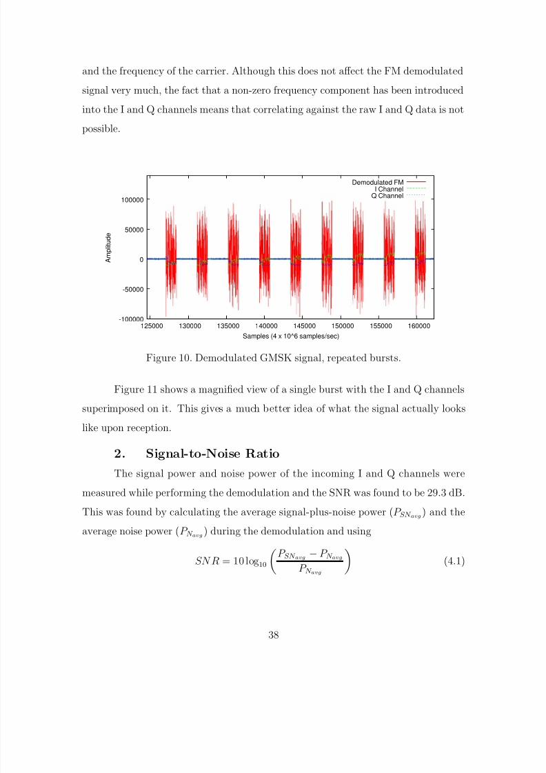
5/12/2018 GetTRDoc - slidepdf.com
http://slidepdf.com/reader/full/gettrdoc-55a35d023bc26 64/116
and the frequency of the carrier. Although this does not affect the FM demodulated
signal very much, the fact that a non-zero frequency component has been introduced
into the I and Q channels means that correlating against the raw I and Q data is not
possible.
-100000
-50000
0
50000
100000
125000 130000 135000 140000 145000 150000 155000 160000
A m p l i t u d e
Samples (4 x 10^6 samples/sec)
Demodulated FMI Channel
Q Channel
Figure 10. Demodulated GMSK signal, repeated bursts.
Figure 11 shows a magnified view of a single burst with the I and Q channels
superimposed on it. This gives a much better idea of what the signal actually looks
like upon reception.
2. Signal-to-Noise Ratio
The signal power and noise power of the incoming I and Q channels were
measured while performing the demodulation and the SNR was found to be 29.3 dB.
This was found by calculating the average signal-plus-noise power (P SN avg) and the
average noise power (P N avg ) during the demodulation and using
SN R = 10 log10
P SN avg − P N avg
P N avg
(4.1)
38
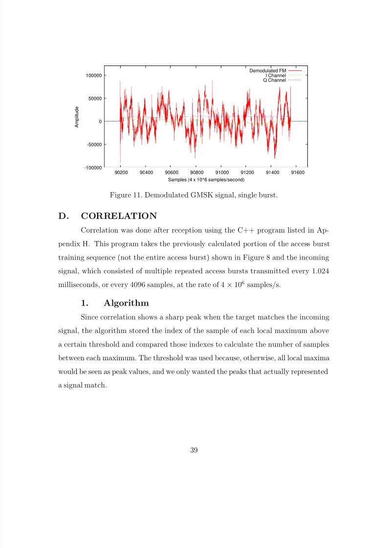
5/12/2018 GetTRDoc - slidepdf.com
http://slidepdf.com/reader/full/gettrdoc-55a35d023bc26 65/116
-100000
-50000
0
50000
100000
90200 90400 90600 90800 91000 91200 91400 91600
A m p l i t u d e
Samples (4 x 10^6 samples/second)
Demodulated FMI Channel
Q Channel
Figure 11. Demodulated GMSK signal, single burst.
D. CORRELATION
Correlation was done after reception using the C++ program listed in Ap-
pendix H. This program takes the previously calculated portion of the access burst
training sequence (not the entire access burst) shown in Figure 8 and the incoming
signal, which consisted of multiple repeated access bursts transmitted every 1.024
milliseconds, or every 4096 samples, at the rate of 4 × 10⁶
samples/s.
1. Algorithm
Since correlation shows a sharp peak when the target matches the incoming
signal, the algorithm stored the index of the sample of each local maximum above
a certain threshold and compared those indexes to calculate the number of samples
between each maximum. The threshold was used because, otherwise, all local maxima
would be seen as peak values, and we only wanted the peaks that actually represented
a signal match.
39
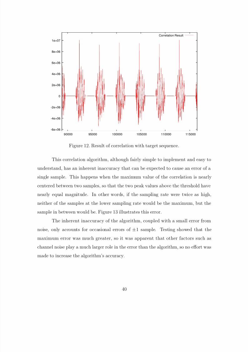
5/12/2018 GetTRDoc - slidepdf.com
http://slidepdf.com/reader/full/gettrdoc-55a35d023bc26 66/116
-6e+06
-4e+06
-2e+06
0
2e+06
4e+06
6e+06
8e+06
1e+07
90000 95000 100000 105000 110000 115000
Correlation Result
Figure 12. Result of correlation with target sequence.
This correlation algorithm, although fairly simple to implement and easy to
understand, has an inherent inaccuracy that can be expected to cause an error of a
single sample. This happens when the maximum value of the correlation is nearly
centered between two samples, so that the two peak values above the threshold have
nearly equal magnitude. In other words, if the sampling rate were twice as high,
neither of the samples at the lower sampling rate would be the maximum, but the
sample in between would be. Figure 13 illustrates this error.
The inherent inaccuracy of the algorithm, coupled with a small error from
noise, only accounts for occasional errors of ±1 sample. Testing showed that the
maximum error was much greater, so it was apparent that other factors such as
channel noise play a much larger role in the error than the algorithm, so no effort was
made to increase the algorithm’s accuracy.
40
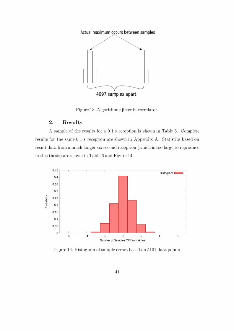
5/12/2018 GetTRDoc - slidepdf.com
http://slidepdf.com/reader/full/gettrdoc-55a35d023bc26 67/116
Figure 13. Algorithmic jitter in correlator.
2. Results
A sample of the results for a 0.1 s reception is shown in Table 5. Complete
results for the same 0.1 s reception are shown in Appendix A. Statistics based on
result data from a much longer six second reception (which is too large to reproduce
in this thesis) are shown in Table 6 and Figure 14.
0
0.05
0.1
0.15
0.2
0.25
0.3
0.35
0.4
0.45
-6 -4 -2 0 2 4 6
P r o b a b i l i t y
Number of Samples Off From Actual
Histogram
Figure 14. Histogram of sample errors based on 5101 data points.
41
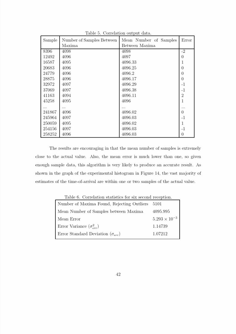
5/12/2018 GetTRDoc - slidepdf.com
http://slidepdf.com/reader/full/gettrdoc-55a35d023bc26 68/116
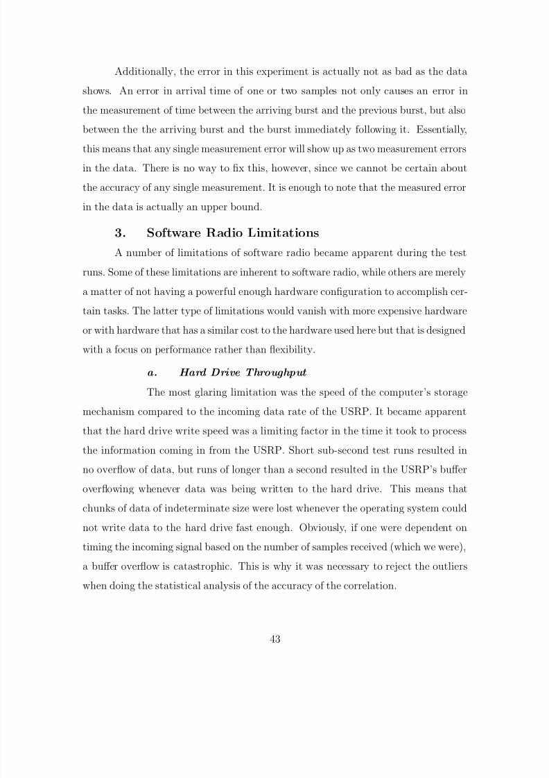
5/12/2018 GetTRDoc - slidepdf.com
http://slidepdf.com/reader/full/gettrdoc-55a35d023bc26 69/116
Additionally, the error in this experiment is actually not as bad as the data
shows. An error in arrival time of one or two samples not only causes an error in
the measurement of time between the arriving burst and the previous burst, but also
between the the arriving burst and the burst immediately following it. Essentially,
this means that any single measurement error will show up as two measurement errors
in the data. There is no way to fix this, however, since we cannot be certain about
the accuracy of any single measurement. It is enough to note that the measured error
in the data is actually an upper bound.
3. Software Radio Limitations
A number of limitations of software radio became apparent during the test
runs. Some of these limitations are inherent to software radio, while others are merely
a matter of not having a powerful enough hardware configuration to accomplish cer-
tain tasks. The latter type of limitations would vanish with more expensive hardware
or with hardware that has a similar cost to the hardware used here but that is designed
with a focus on performance rather than flexibility.
a. Hard Drive Throughput
The most glaring limitation was the speed of the computer’s storage
mechanism compared to the incoming data rate of the USRP. It became apparent
that the hard drive write speed was a limiting factor in the time it took to process
the information coming in from the USRP. Short sub-second test runs resulted in
no overflow of data, but runs of longer than a second resulted in the USRP’s buffer
overflowing whenever data was being written to the hard drive. This means that
chunks of data of indeterminate size were lost whenever the operating system could
not write data to the hard drive fast enough. Obviously, if one were dependent on
timing the incoming signal based on the number of samples received (which we were),
a buffer overflow is catastrophic. This is why it was necessary to reject the outliers
when doing the statistical analysis of the accuracy of the correlation.
43
5/12/2018 GetTRDoc - slidepdf.com
http://slidepdf.com/reader/full/gettrdoc-55a35d023bc26 70/116
b. Processing Speed
The next limitation, which the test data does not show, is that the
processing speed of a general-purpose CPU is not fast enough to perform the FM
demodulation and correlation in real time. Although the correlator.cpp programused to perform the correlation was not highly optimized for this problem, its run
time still gives us a good idea of the scale of the problem. For a 0.1 second reception,
the correlation took over two seconds to perform, a factor of 20. Only a cluster of the
fastest general purpose CPUs can keep up with the incoming data rate in this case.
Reduction of the decimation rate from 16 to eight or lower in order to get a more
accurate result compounds this problem.
Until general-purpose CPU speeds become much faster, the real-time
FM demodulation and correlation portion of the software radio is much more effec-
tively performed by a special-purpose processor, high performance DSP, or FPGA.
c. USB Data Rate
The USB data rate, although theoretically able to provide up to 8×10⁶
samples/s, worked much better with a decimation rate of 16, which corresponds to
an incoming rate of 4 × 10⁶ complex samples/second. A decimation rate of eight
was found to result in too many buffer overflows to be usable for estimating thetime-of-arrival. Even if the system were capable of handling a decimation rate of
eight, not having to do decimation at all would mean a much greater potential to
accurately determine arrival time. A software radio receiver that used a higher data
rate connection, like Gigabit Ethernet or PCI, would be capable of providing a higher
data rate. Again, this would likely result in hardware that is more expensive and less
flexible than the USRP, so this limitation should be seen as a trade-off.
E. LOCATING THE EMITTER
Unfortunately, the precision achieved using the USRP did not allow testing
using multiple USRPs as receivers to see how accurately they could locate an emitter.
44
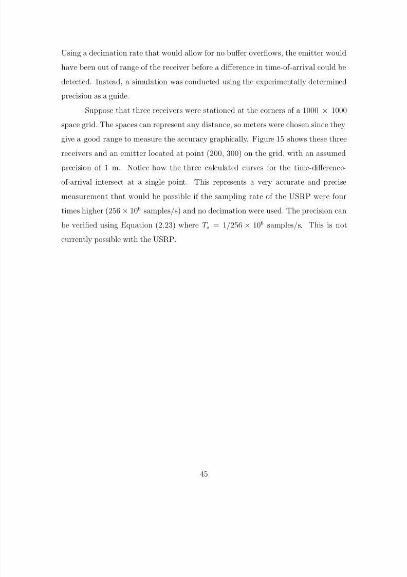
5/12/2018 GetTRDoc - slidepdf.com
http://slidepdf.com/reader/full/gettrdoc-55a35d023bc26 71/116
Using a decimation rate that would allow for no buffer overflows, the emitter would
have been out of range of the receiver before a difference in time-of-arrival could be
detected. Instead, a simulation was conducted using the experimentally determined
precision as a guide.
Suppose that three receivers were stationed at the corners of a 1000 × 1000
space grid. The spaces can represent any distance, so meters were chosen since they
give a good range to measure the accuracy graphically. Figure 15 shows these three
receivers and an emitter located at point (200, 300) on the grid, with an assumed
precision of 1 m. Notice how the three calculated curves for the time-difference-
of-arrival intersect at a single point. This represents a very accurate and precise
measurement that would be possible if the sampling rate of the USRP were four
times higher (256 × 106 samples/s) and no decimation were used. The precision can
be verified using Equation (2.23) where T s = 1/256 × 106 samples/s. This is not
currently possible with the USRP.
45
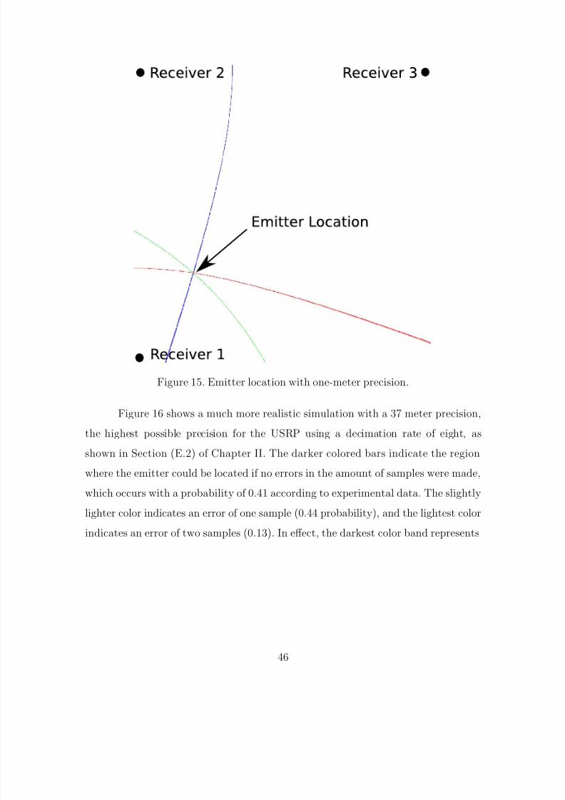
5/12/2018 GetTRDoc - slidepdf.com
http://slidepdf.com/reader/full/gettrdoc-55a35d023bc26 72/116
Figure 15. Emitter location with one-meter precision.
Figure 16 shows a much more realistic simulation with a 37 meter precision,the highest possible precision for the USRP using a decimation rate of eight, as
shown in Section (E.2) of Chapter II. The darker colored bars indicate the region
where the emitter could be located if no errors in the amount of samples were made,
which occurs with a probability of 0.41 according to experimental data. The slightly
lighter color indicates an error of one sample (0.44 probability), and the lightest color
indicates an error of two samples (0.13). In effect, the darkest color band represents
46
5/12/2018 GetTRDoc - slidepdf.com
http://slidepdf.com/reader/full/gettrdoc-55a35d023bc26 73/116
the inherent 37 meter imprecision of the system based on Equation (2.23) and each
successively lighter color band around it represents another 37 meter (or single sample)
imprecision. Based on the experimental histogram shown in Figure 14, the emitter
would be located within the intersection of the colored curves more than 98% of the
time.
Figure 16. Emitter location with 37-meter precision.
F. CONCLUSION
At this point, the implementation of the software radio has been tested and
has shown to be reasonably precise, such that it could be used in applications where
pinpoint accuracy is not required. This chapter has shown that minor modifications
to the hardware specifications could result in a much greater accuracy and precision
47

5/12/2018 GetTRDoc - slidepdf.com
http://slidepdf.com/reader/full/gettrdoc-55a35d023bc26 74/116
using the same algorithms. The following chapter discusses the conclusions that can
be taken from this research and the possible directions future research could take.
48
5/12/2018 GetTRDoc - slidepdf.com
http://slidepdf.com/reader/full/gettrdoc-55a35d023bc26 75/116
V. CONCLUSION
A. CONCLUSIONS
This research has shown that performing geolocation of a GSM signal usingsoftware defined radio is possible, and even accurate, with some caveats. The USRP
is a very low-cost device that was designed for flexibility rather than performance
but has the potential to perform a geolocation with an 80 meter radius in over 98
percent of the test cases. This is certainly good enough for applications where pinpoint
accuracy is not required. The accuracy and precision can be much greater with minor
changes in hardware.
The most important limitation is the slow speed of general-purpose hardwarethat necessitates performing the analysis of received data in non-real time, which
creates other limitations having to do with lack of fast storage space, processing power,
etc. This points to the need to push more functionality out from software and onto
the hardware, which would reduce the flexibility. However, by using reconfigurable,
programmable hardware like FGPAs, most of the benefits of software radio would be
retained while still gaining the performance required for real-time operation.
B. RECOMMENDATIONS
Time constraints precluded taking the next step in improving this system,
which would be to alter the code on the USRP’s FPGA to perform the correlation
of the target signal with the received data in hardware instead of in software. That
way, the USRP could simply send the number of samples and the correlation data
instead of sending the raw samples to the computer for processing. Additionally, since
the FPGA performs the decimation of the signal by default, this could be changed
such that no decimation occurred prior to the correlation. This would allow for an
accuracy of about 5 meters using only the USRP.
49
5/12/2018 GetTRDoc - slidepdf.com
http://slidepdf.com/reader/full/gettrdoc-55a35d023bc26 76/116
The idea of performing correlation of the I and Q signals without performing
the FM demodulation could work if either an RF front-end were developed that could
exactly match the carrier frequency and phase or if the phase and frequency error
between the carrier and the receiver were to be corrected in software. Correction of
the phase and frequency of the received I and Q signals in software may turn out to be
more computationally expensive than simply doing the FM demodulation. However,
time constraints prevent exploration of this more fully.
Finally, the USRP is not the only hardware platform that can be used to im-
plement a software radio. The algorithms and software developed in this thesis could
be used nearly unchanged with more powerful hardware to get much better results.
Specifically, an RF front-end and antenna developed specifically for the reception of
GSM signals would likely perform much better for the reception of that signal than
the USRP daughter-board designed with a range of signals in mind.
50
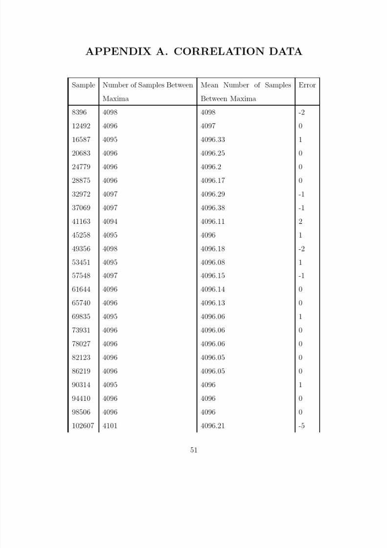
5/12/2018 GetTRDoc - slidepdf.com
http://slidepdf.com/reader/full/gettrdoc-55a35d023bc26 77/116
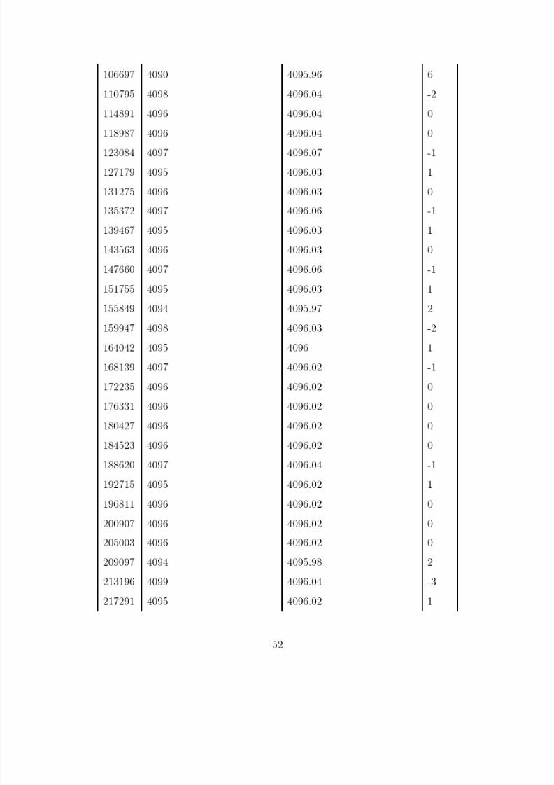
5/12/2018 GetTRDoc - slidepdf.com
http://slidepdf.com/reader/full/gettrdoc-55a35d023bc26 78/116
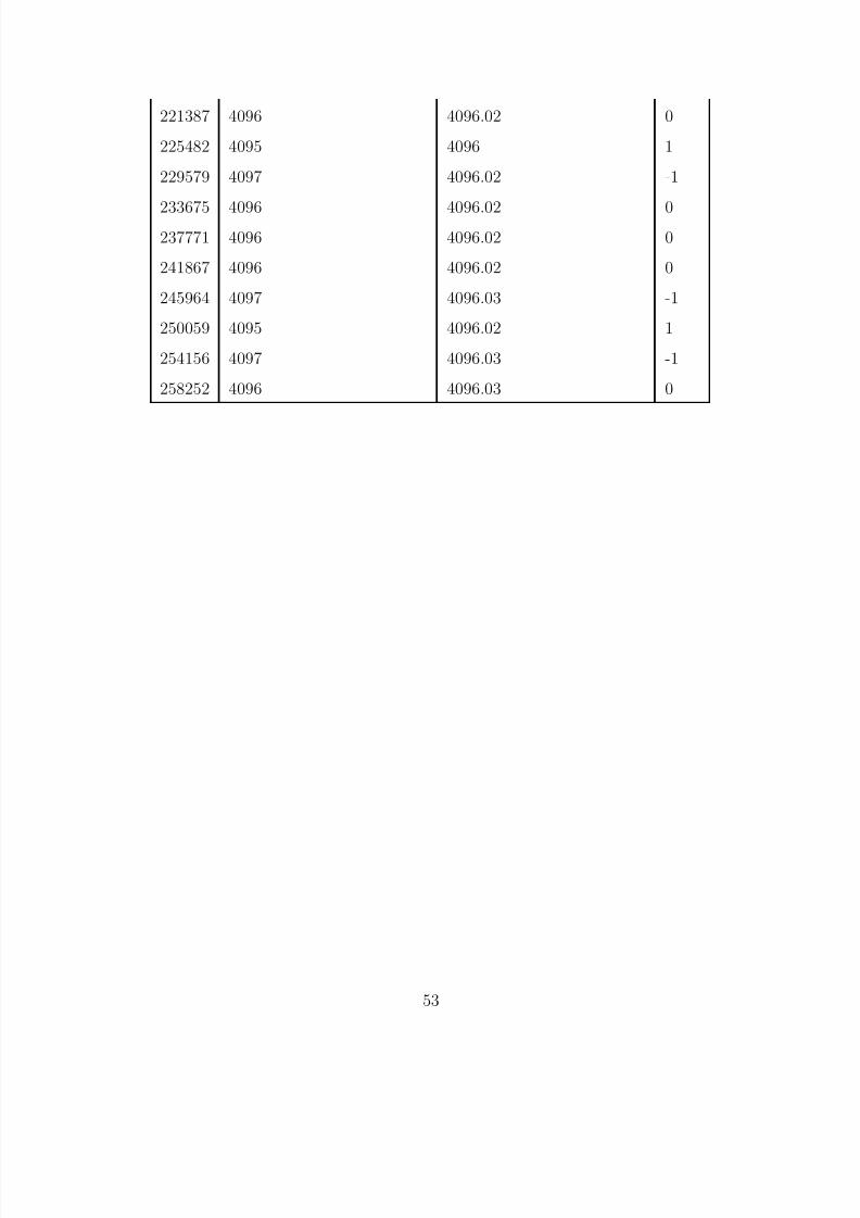
5/12/2018 GetTRDoc - slidepdf.com
http://slidepdf.com/reader/full/gettrdoc-55a35d023bc26 79/116
221387 4096 4096.02 0
225482 4095 4096 1
229579 4097 4096.02 -1
233675 4096 4096.02 0237771 4096 4096.02 0
241867 4096 4096.02 0
245964 4097 4096.03 -1
250059 4095 4096.02 1
254156 4097 4096.03 -1
258252 4096 4096.03 0
53

5/12/2018 GetTRDoc - slidepdf.com
http://slidepdf.com/reader/full/gettrdoc-55a35d023bc26 80/116
THIS PAGE INTENTIONALLY LEFT BLANK
54
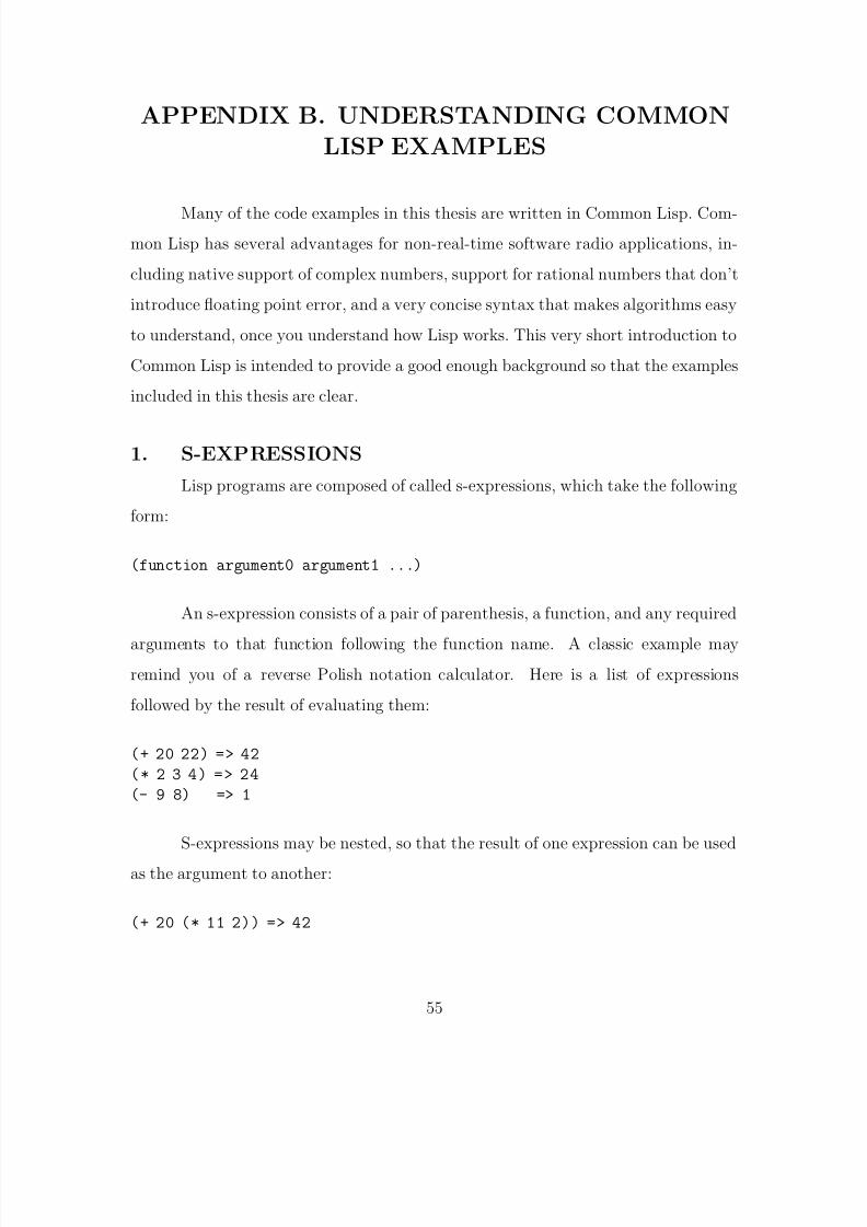
5/12/2018 GetTRDoc - slidepdf.com
http://slidepdf.com/reader/full/gettrdoc-55a35d023bc26 81/116
APPENDIX B. UNDERSTANDING COMMON
LISP EXAMPLES
Many of the code examples in this thesis are written in Common Lisp. Com-
mon Lisp has several advantages for non-real-time software radio applications, in-
cluding native support of complex numbers, support for rational numbers that don’t
introduce floating point error, and a very concise syntax that makes algorithms easy
to understand, once you understand how Lisp works. This very short introduction to
Common Lisp is intended to provide a good enough background so that the examples
included in this thesis are clear.
1. S-EXPRESSIONS
Lisp programs are composed of called s-expressions, which take the following
form:
(function argument0 argument1 ...)
An s-expression consists of a pair of parenthesis, a function, and any required
arguments to that function following the function name. A classic example may
remind you of a reverse Polish notation calculator. Here is a list of expressions
followed by the result of evaluating them:
(+ 20 22) => 42
(* 2 3 4) => 24
(- 9 8) => 1
S-expressions may be nested, so that the result of one expression can be used
as the argument to another:
(+ 20 (* 11 2)) => 42
55
5/12/2018 GetTRDoc - slidepdf.com
http://slidepdf.com/reader/full/gettrdoc-55a35d023bc26 82/116
For the most part, Lisp programs consist of a series of nested s-expressions
that are evaluated sequentially. The result of a Lisp program (or function) is the
value returned by the final s-expression.
Lisp has quite a few built-in functions, but wouldn’t be very useful unless
you could define your own. This is done using what is called a special form in Lisp,
specifically the special form defun. Suppose we want a function that takes a single
argument and adds 3 to it:
(defun add3 (x)
(+ x 3))
The first part of the defun form is the word defun, which indicates that we’re
defining a function. The second item is the name of the function. The third part
is a list of arguments, enclosed in parentheses. The reason defun is called a special
form is because the argument list is not evaluated, as an s-expression would be. It’s
treated differently. The last part of the defun form is called the body, and consists of
a series of s-expressions, the last of which produces the result of the function.
The argument list contains a symbol used to represent the value that will be
passed into add3 when it is called. The final (and only) s-expression in the add3
defun is (+ x 3), so the add3 function will return this value as its result:
(add3 4) => 7
Just as in most other programming languages, in Lisp it may become necessary
to define local variables, which are variables which only have meaning within the scope
of the function. This is done with another special form, called let:
(defun add-stuff (x)
(let ((y 4)
(z 5))
(+ x 3)))
56
5/12/2018 GetTRDoc - slidepdf.com
http://slidepdf.com/reader/full/gettrdoc-55a35d023bc26 83/116
Let works just like the mathematical term, in that it assigns a value to a symbol
(or multiple symbols.) That assignment exists everywhere inside the parentheses that
began the let form, so this is valid syntax:
(let ((a 0))
(defun get-a ()
a)
(defun set-a (x)
(setf a x)))
The preceding code defined two functions that had access to the a symbol,
get-a and set-a. Executing (set-a 4) followed by (get-a) would return the value
4.
Since everything in Common Lisp is an s-expression, the preceding covered just
about all that is necessary to know about the syntax of Common Lisp to understand
the code included in this thesis.
57

5/12/2018 GetTRDoc - slidepdf.com
http://slidepdf.com/reader/full/gettrdoc-55a35d023bc26 84/116
THIS PAGE INTENTIONALLY LEFT BLANK
58
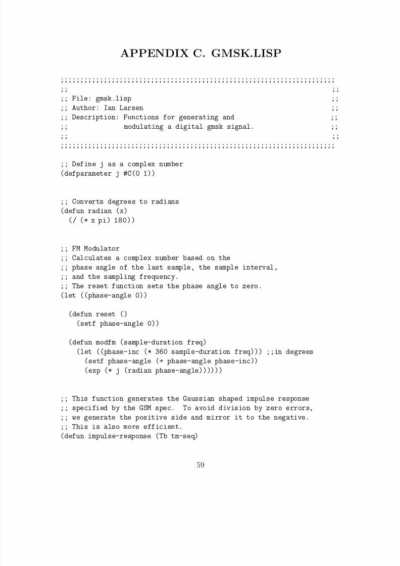
5/12/2018 GetTRDoc - slidepdf.com
http://slidepdf.com/reader/full/gettrdoc-55a35d023bc26 85/116
APPENDIX C. GMSK.LISP
;;;;;;;;;;;;;;;;;;;;;;;;;;;;;;;;;;;;;;;;;;;;;;;;;;;;;;;;;;;;;;;;;;;;;;
;; ;;
;; File: gmsk.lisp ;;;; Author: Ian Larsen ;;
;; Description: Functions for generating and ;;
;; modulating a digital gmsk signal. ;;
;; ;;
;;;;;;;;;;;;;;;;;;;;;;;;;;;;;;;;;;;;;;;;;;;;;;;;;;;;;;;;;;;;;;;;;;;;;;
;; Define j as a complex number
(defparameter j #C(0 1))
;; Converts degrees to radians
(defun radian (x)
(/ (* x pi) 180))
;; FM Modulator
;; Calculates a complex number based on the
;; phase angle of the last sample, the sample interval,
;; and the sampling frequency.
;; The reset function sets the phase angle to zero.
(let ((phase-angle 0))
(defun reset ()
(setf phase-angle 0))
(defun modfm (sample-duration freq)
(let ((phase-inc (* 360 sample-duration freq))) ;;in degrees
(setf phase-angle (+ phase-angle phase-inc))
(exp (* j (radian phase-angle))))))
;; This function generates the Gaussian shaped impulse response;; specified by the GSM spec. To avoid division by zero errors,
;; we generate the positive side and mirror it to the negative.
;; This is also more efficient.
(defun impulse-response (Tb tm-seq)
59
5/12/2018 GetTRDoc - slidepdf.com
http://slidepdf.com/reader/full/gettrdoc-55a35d023bc26 86/116
(let* ((delta (/ (sqrt (log 2)) (* 2 pi 0.3)))
(response (map ’array
(lambda (tm)
(/
(exp (/
(* -1 (expt tm 2))(* 2 (expt delta 2) (expt Tb 2))))
(* (sqrt (* 2 pi)) delta Tb)))
tm-seq)))
(concatenate ’array
(reverse response)
response)))
;; Takes a stream of bits and outputs a differentially
;; encoded stream of the same length. The optional last
;; parameter allows us to specify what the state of the
;; prior encoded bit should be. It defaults to 1, in
;; compliance with the GSM spec, which states the differential
;; encoder’s state at the start of encoding should be as if
;; a series of 1’s had just been encoded.
(defun diff-encoder (bits &optional (last 1))
(let ((p last))
(map ’array (lambda (x)
(let ((d (logxor x p)))
(setf p x)
(- 1 (* 2 d))))bits)))
;; Takes a list of bits and returns the same bitstream,
;; with the bits repeating n times.
;; This is how we generate rectangular symbols from impulses.
(defun make-bitstream (bits n)
(let ((result #()))
(map nil (lambda (x)
(setf result
(concatenate
’array
result
(make-array n :initial-element x))))
(diff-encoder bits))
60
5/12/2018 GetTRDoc - slidepdf.com
http://slidepdf.com/reader/full/gettrdoc-55a35d023bc26 87/116
result))
;; Make a sequence of numbers, starting with starnum,
;; and incrementing by increment. Defaults to 1 as the
;; increment. Similar to Matlab’s linspace function.(defun make-seq (startnum length &optional (increment 1))
(let ((a (make-array length :initial-element startnum)))
(map ’array (let ((acc (- increment)))
(lambda (y)
(setf acc (+ acc increment))
(+ y acc)))
a)))
;; Generate the gmsk Gaussian filter based on values
;; in the GSM spec.
(defun gsm-gmsk (sample-interval)
(let* ((Tb 6/1625000) ;; bit duration
(BTb 0.3) ;; bandwidth time product
(B (/ BTb Tb))
(filter-length
(* 2 (/ Tb sample-interval)))) ;;should be an integer
(format t "Filter length: ~a~%" filter-length)
(impulse-response
Tb (make-seq 0 filter-length sample-interval))))
;; This will take an array of numbers, find the
;; absolute maximum, and divide all numbers by that.
;; This is a linear scaling normalization.
(defun normalize (l)
(let ((max (abs (reduce (lambda (a b)
(if (> (abs a) (abs b))
(abs a)
(abs b)))
l))))
(if (> max 0)
(map ’array
(lambda (x)
(/ x max))
l)
61
5/12/2018 GetTRDoc - slidepdf.com
http://slidepdf.com/reader/full/gettrdoc-55a35d023bc26 88/116
l)))
;; Perform convolution of stream and base.
;; base should be longer than stream.
(defun convolve (stream base)(let* ((len (length stream))
(iter (+ (length stream) (length base) -1))
(result (make-array iter :initial-element 0)))
(dotimes (count iter nil)
(setf (aref result count)
(reduce #’+
(map ’array
(lambda (r s)
(* r s))
(if (> len count)
(subseq stream (- len count 1))
stream)
(if (> len count)
base
(subseq base (- count len -1)))))))
result))
;; Return an array of every "rate" samples from array x.
(defun decimate (x rate)
(let ((result ()))(loop for i from 0 to (1- (length x)) do
(if (eq (mod i rate) 0)
(setf result
(concatenate ’array result (list (aref x i))))))
result))
;;; This sets everything in motion (main procedure)
;; results are stored in the four files, filt.dat, gauss.dat,
;; bitstream.dat, and gmsk.asc
;; gmsk.asc is the final signal that we’ll be sending, the rest
;; make nice graphs so you can see what’s happening at each stage.
(let* ((filtout (open "filt.dat" :direction :output
:if-exists :supersede :if-does-not-exist :create))
62
5/12/2018 GetTRDoc - slidepdf.com
http://slidepdf.com/reader/full/gettrdoc-55a35d023bc26 89/116
(gaussout (open "gauss.dat" :direction :output
:if-exists :supersede :if-does-not-exist :create))
(bitsout (open "bitstream.dat" :direction :output
:if-exists :supersede :if-does-not-exist :create))
(gmskout (open "gmsk.asc" :direction :output
:if-exists :supersede :if-does-not-exist :create))(buffer-size 4096) ;;number of samples in gmsk.asc
(Rs 52000000) ;;Fast sample rate that we decimate later
(Ts (/ 1 Rs)) ;;Sample duration
(n0 13) ;;Decimation rate to get 4x10^6 samples/sec
(n1 192) ;;Number of times we repeat each bit
(delta 1625000/24) ;;1/4 270.833333 as per GSM spec (Rappaport pg 566
(mag 30000)) ;;amplitude
(reset) ;;Sets phase angle to zero
(let* ((filter (gsm-gmsk Ts)) ;;make gaussian filter
(bits (make-bitstream ;; create the access burst bits
’(0 0 1 1 1 0 1 0 ;;extended tail bits
0 1 0 0 1 ;;training sequence: 41 bits
0 1 1 0 1
1 1 1 1 1
1 1 0 0 1
1 0 0 1 1
0 1 0 1 0
1 0 0 0 1
1 1 1 0 0 0
0 1 0 1 1 0;;encrypted bits: 36 bits
0 1 0 1 1 0
1 0 1 1 0 0
0 0 1 0 0 1
1 0 0 1 0 1
0 1 0 1 1 1
0 0 0 ;;tail bits
) n1))
;; now filter the access burst
(filtered (normalize (convolve filter bits)))
;; decimate to get proper sample rate
(modwave (decimate filtered n0))
;; create padding for 4096 samples
63
5/12/2018 GetTRDoc - slidepdf.com
http://slidepdf.com/reader/full/gettrdoc-55a35d023bc26 90/116
(zerobuffer (make-array
(* (ceiling (/
(- buffer-size
(length modwave))
2))
2):initial-element 0)))
;; Write gaussian filter to file
(map nil (lambda (x)
(format gaussout "~A~%" x))
(normalize filter))
;; Write raw bits to file
(map nil (lambda (x)
(format bitsout "~A~%" x))
bits)
;; Write filtered bits to file
(map nil (lambda (x)
(format filtout "~A~%" x))
modwave)
;; Write GMSK signal with zero padding
(map nil (lambda (x)
(format gmskout "~A~%" x))
zerobuffer)(map nil (lambda (x)
(let ((complex (modfm Ts (* delta x))))
(format gmskout "~f~%~f~%"
(* mag (realpart complex))
(* mag (imagpart complex)))))
modwave)
(map nil (lambda (x)
(format gmskout "~A~%" x))
zerobuffer)
;; Close files, and we’re done.
(close filtout)
(close gaussout)
(close bitsout)
(close gmskout)))
64
5/12/2018 GetTRDoc - slidepdf.com
http://slidepdf.com/reader/full/gettrdoc-55a35d023bc26 91/116
APPENDIX D. TRANSMIT.PY
#!/usr/bin/python
########################################### File: transmit.py #
# Author: Ian Larsen #
# Description: Uses the gnuradio python #
# module to tune the USRP and transmit #
# the raw GMSK I/Q data to it. #
# #
##########################################
from gnuradio import gr
from gnuradio import usrp
def build_graph ():
fg = gr.flow_graph ()
#set the USRP as our destination
dest = usrp.sink_c(0, 32) #32 is the interpolation rate
print "Interp rate: " + str(dest.interp_rate())
print "DAC Freq: " + str(dest.dac_freq())
print "N Channels: " + str(dest.set_nchannels(1))
#Tune the USRP and daughterboard to the proper frequency
subdev = usrp.selected_subdev(dest, (0, 0))
print dest.pga_min()
print dest.pga_max()
dest.set_pga(0, -0.0) #20 dB of gain
dest.set_pga(1, -0.0) #20 dB of gain
print dest.pga(0)
print dest.pga(1)
freq = dest.tune(0, subdev, 900e6)
if freq:print "Frequency: 900e6"
#set up the gmsk data as the source
src = gr.file_source(gr.sizeof_gr_complex, "gmsk.bin", True)
65
5/12/2018 GetTRDoc - slidepdf.com
http://slidepdf.com/reader/full/gettrdoc-55a35d023bc26 92/116
#connect the source to the destination
fg.connect (src, dest)
return fg
#main loop
if __name__ == ’__main__’:
fg = build_graph ()
fg.start ()
raw_input (’Press Enter to quit: ’)
fg.stop ()
66
5/12/2018 GetTRDoc - slidepdf.com
http://slidepdf.com/reader/full/gettrdoc-55a35d023bc26 93/116
APPENDIX E. RECEIVE.PY
#!/usr/bin/python
############################################# File: receive.py #
# Author: Ian Larsen #
# Description: Uses the gnuradio python #
# module to tune the USRP and receive #
# the raw GMSK I/Q data from it, #
# demodulate it using an FM demodulator, #
# and store the result in file "fmraw.dat" #
# #
############################################
from gnuradio import gr
from gnuradio import usrp
import time
def build_graph ():
#set decimation rate and center frequency
decim = 16
center_freq = 900e6
#build flow graph
# this is simple, it comes in from the USRP,
# into the demodulator, and out to a file.
fg = gr.flow_graph ()
u = usrp.source_c(0, decim)
#select the flex900 daughterboard
subdev = usrp.selected_subdev(u, (0,0))
g = subdev.gain_range()
#set the gain and tune
subdev.set_gain((g[0] + g[1]) * 0.5)
freq = u.tune(0, subdev, center_freq)
67
5/12/2018 GetTRDoc - slidepdf.com
http://slidepdf.com/reader/full/gettrdoc-55a35d023bc26 94/116
#define the components
sink0 = gr.file_sink(gr.sizeof_float, "fmraw.dat")
demod = gr.quadrature_demod_cf(4)
#connect the components
fg.connect (u, demod)fg.connect (demod, sink0)
#return completed flow graph
return fg
# Main - only receive for 0.2 seconds, otherwise
# we’ll get a huge amount of data
if __name__ == ’__main__’:
fg = build_graph ()
fg.start ()
time.sleep(0.2)
fg.stop ()
68
5/12/2018 GetTRDoc - slidepdf.com
http://slidepdf.com/reader/full/gettrdoc-55a35d023bc26 95/116
APPENDIX F. RECEIVE2.PY
#!/usr/bin/python
############################################# File: receive2.py #
# Author: Ian Larsen #
# Description: Uses the gnuradio python #
# module to tune the USRP and receive #
# the raw GMSK I/Q data from it, #
# and store the result in file "fmraw.dat" #
# #
############################################
from gnuradio import gr
from gnuradio import usrp
import time
def build_graph ():
# set decimation rate and center frequency
decim = 16
center_freq = 900e6
#build flow graph
fg = gr.flow_graph ()
u = usrp.source_c(0, decim)
#get access to flex900 daughterboard
subdev = usrp.selected_subdev(u, (0,0))
#set gain and tune
g = subdev.gain_range()
subdev.set_gain((g[0] + g[1]) * 0.5)
freq = u.tune(0, subdev, center_freq)
#generate component - just a file sink here.
sink0 = gr.file_sink(gr.sizeof_gr_complex, "fmraw.dat")
69
5/12/2018 GetTRDoc - slidepdf.com
http://slidepdf.com/reader/full/gettrdoc-55a35d023bc26 96/116
#connect output of USRP straight to file
fg.connect (u, sink0)
#return the flow graph
return fg
# Main - only receive for 0.1 second, otherwise
# we’ll get a huge amount of data
if __name__ == ’__main__’:
fg = build_graph ()
fg.start ()
time.sleep(0.1)
fg.stop ()
70
5/12/2018 GetTRDoc - slidepdf.com
http://slidepdf.com/reader/full/gettrdoc-55a35d023bc26 97/116
APPENDIX G. FM DEMOD.PL
#!/usr/bin/perl
########################################### File: fm_demod.pl #
# Author: Ian Larsen #
# Description: Reads 8-byte binary #
# complex IQ samples stored by gnuradio #
# and demodulates them as an FM signal. #
# Signal power is measured in order to #
# decide when an FM signal is being #
# received, as opposed to just noise. #
# A limiter is employed to eliminate #
# transients that occur when the FM #
# demodulator is turned on and off. #
# #
##########################################
use strict;
#open input and output files
open(INFILE, shift) or die "Couldn’t open input file.\n";
my $outname = shift or die "Couldn’t open output file.\n";
open(FMOUT, ">$outname.fm") or die "Couldn’t open output file.\n";
open(FMBIN, ">$outname.bin") or die "Couldn’t open output file.\n";open(IOUT, ">$outname.i") or die "Couldn’t open output file.\n";
open(QOUT, ">$outname.q") or die "Couldn’t open output file.\n";
#set decimation rate, 16 is default.
my $decim = shift || 16;
# Find sample duration based on decimation rate
my $dt = 1 / (64000000 / $decim);
print "Sample interval: $dt\n";
my $oldI = 0;
my $oldQ = 0; my $power = 0;
my $thresholdPower = 1e13; #130dB
my $signalNoisePower = 0;
my $signalTime = 0;
71
5/12/2018 GetTRDoc - slidepdf.com
http://slidepdf.com/reader/full/gettrdoc-55a35d023bc26 98/116
my $noisePower = 0;
my $noiseTime = 0;
my $data;
# Read an IQ sample, one at a time
while (read(INFILE, $data, 8))
# translate binary float data into
# a form we can use
my ($i, $q) = unpack("ff", $data);
# write IQ samples to files
print IOUT "$i\n";
print QOUT "$q\n";
# Avoid division by zero
if ($i == 0)
$i = 0.0001;
if ($q == 0)
$q = 0.0001;
my $fm = 0;
# Check signal power.
# If it’s over the threshold, we demodulate
# by differentiating the phase to get
# instantaneous frequency.
# Otherwise, we output a zero.
$power = ($i * $i + $q * $q) / $dt;
if ($power > $thresholdPower)
$fm = (($i * ($q - $oldQ) / $dt) -
($q * ($i - $oldI) / $dt)) /
(($i *$i) + ($q * $q));
if ($fm > 100000 || $fm < -100000)
$fm = 0;
72
5/12/2018 GetTRDoc - slidepdf.com
http://slidepdf.com/reader/full/gettrdoc-55a35d023bc26 99/116
# Keep track of total signal power
# for SNR meausurement
$signalNoisePower += $power;
$signalTime += $dt;
else
# Keep track of total noise power
# for SNR meausurement
$noisePower += $power;
$noiseTime += $dt;
# Write output to files
print FMOUT "$fm\n";
print FMBIN pack("f", $fm);
$oldI = $i;
$oldQ = $q;
#print results
my $avgSNP = ($signalNoisePower / $signalTime);
my $avgNP = ($noisePower / $noiseTime);
print "Average signal plus noise power: $avgSNP \n";
print "Average noise power: $avgNP \n";
print "Calculated average signal power: " . ( $avgSNP - $avgNP ) . "\n";print "SNR: " . (($avgSNP - $avgNP) / $avgNP) . "\n";
close INFILE;
close FMOUT;
close FMBIN;
close IOUT;
close QOUT;
73

5/12/2018 GetTRDoc - slidepdf.com
http://slidepdf.com/reader/full/gettrdoc-55a35d023bc26 100/116
THIS PAGE INTENTIONALLY LEFT BLANK
74
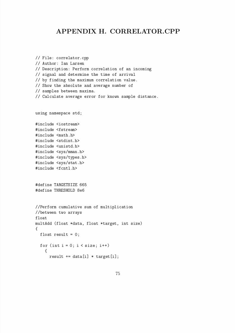
5/12/2018 GetTRDoc - slidepdf.com
http://slidepdf.com/reader/full/gettrdoc-55a35d023bc26 101/116
APPENDIX H. CORRELATOR.CPP
// File: correlator.cpp// Author: Ian Larsen
// Description: Perform correlation of an incoming
// signal and determine the time of arrival
// by finding the maximum correlation value.
// Show the absolute and average number of
// samples between maxima.
// Calculate average error for known sample distance.
using namespace std;
#include <iostream>
#include <fstream>
#include <math.h>
#include <stdint.h>
#include <unistd.h>
#include <sys/mman.h>
#include <sys/types.h>
#include <sys/stat.h>
#include <fcntl.h>
#define TARGETSIZE 665
#define THRESHOLD 8e6
//Perform cumulative sum of multiplication
//between two arrays
float
multAdd (float *data, float *target, int size)
float result = 0;
for (int i = 0; i < size; i++)
result += data[i] * target[i];
75
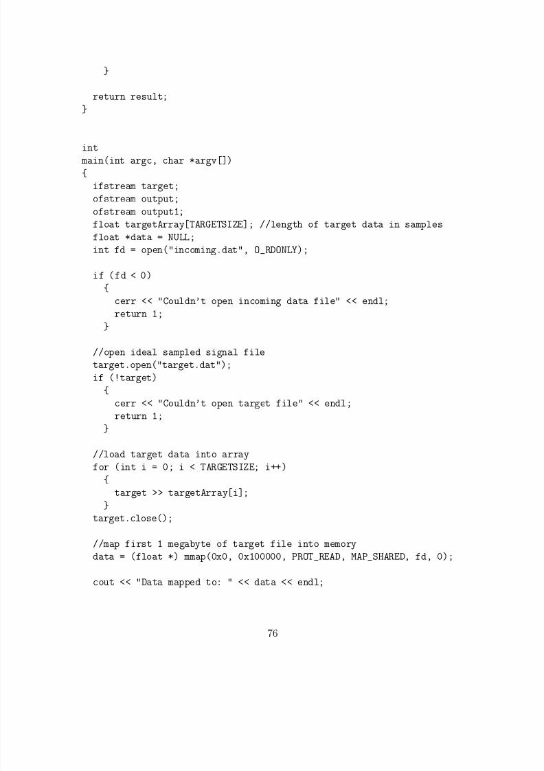
5/12/2018 GetTRDoc - slidepdf.com
http://slidepdf.com/reader/full/gettrdoc-55a35d023bc26 102/116
return result;
int
main(int argc, char *argv[])
ifstream target;
ofstream output;
ofstream output1;
float targetArray[TARGETSIZE]; //length of target data in samples
float *data = NULL;
int fd = open("incoming.dat", O_RDONLY);
if (fd < 0)
cerr << "Couldn’t open incoming data file" << endl;
return 1;
//open ideal sampled signal file
target.open("target.dat");
if (!target)
cerr << "Couldn’t open target file" << endl;return 1;
//load target data into array
for (int i = 0; i < TARGETSIZE; i++)
target >> targetArray[i];
target.close();
//map first 1 megabyte of target file into memory
data = (float *) mmap(0x0, 0x100000, PROT_READ, MAP_SHARED, fd, 0);
cout << "Data mapped to: " << data << endl;
76
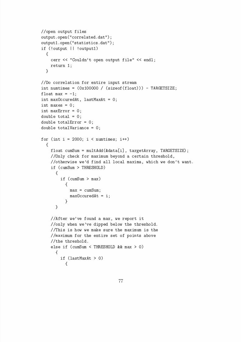
5/12/2018 GetTRDoc - slidepdf.com
http://slidepdf.com/reader/full/gettrdoc-55a35d023bc26 103/116
//open output files
output.open("correlated.dat");
output1.open("statistics.dat");
if (!output || !output1)
cerr << "Couldn’t open output file" << endl;return 1;
//Do correlation for entire input stream
int numtimes = (0x100000 / (sizeof(float))) - TARGETSIZE;
float max = -1;
int maxOccuredAt, lastMaxAt = 0;
int maxes = 0;
int maxError = 0;
double total = 0;
double totalError = 0;
double totalVariance = 0;
for (int i = 2000; i < numtimes; i++)
float cumSum = multAdd(&data[i], targetArray, TARGETSIZE);
//Only check for maximum beyond a certain threshold,
//otherwise we’d find all local maxima, which we don’t want.
if (cumSum > THRESHOLD)
if (cumSum > max)
max = cumSum;
maxOccuredAt = i;
//After we’ve found a max, we report it
//only when we’ve dipped below the threshold.
//This is how we make sure the maximum is the
//maximum for the entire set of points above
//the threshold.
else if (cumSum < THRESHOLD && max > 0)
if (lastMaxAt > 0)
77
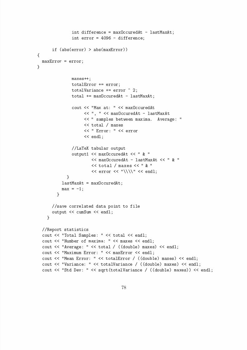
5/12/2018 GetTRDoc - slidepdf.com
http://slidepdf.com/reader/full/gettrdoc-55a35d023bc26 104/116
int difference = maxOccuredAt - lastMaxAt;
int error = 4096 - difference;
if (abs(error) > abs(maxError))
maxError = error;
maxes++;
totalError += error;
totalVariance += error ^ 2;
total += maxOccuredAt - lastMaxAt;
cout << "Max at: " << maxOccuredAt
<< ", " << maxOccuredAt - lastMaxAt
<< " samples between maxima. Average: "
<< total / maxes
<< " Error: " << error
<< endl;
//LaTeX tabular output
output1 << maxOccuredAt << " & "
<< maxOccuredAt - lastMaxAt << " & "
<< total / maxes << " & "
<< error << "\\\\" << endl;
lastMaxAt = maxOccuredAt; max = -1;
//save correlated data point to file
output << cumSum << endl;
//Report statistics
cout << "Total Samples: " << total << endl;
cout << "Number of maxima: " << maxes << endl;
cout << "Average: " << total / ((double) maxes) << endl;
cout << "Maximum Error: " << maxError << endl;
cout << "Mean Error: " << totalError / ((double) maxes) << endl;
cout << "Variance: " << totalVariance / ((double) maxes) << endl;
cout << "Std Dev: " << sqrt(totalVariance / ((double) maxes)) << endl;
78

5/12/2018 GetTRDoc - slidepdf.com
http://slidepdf.com/reader/full/gettrdoc-55a35d023bc26 105/116
output.close();
output1.close();
return 0;
79

5/12/2018 GetTRDoc - slidepdf.com
http://slidepdf.com/reader/full/gettrdoc-55a35d023bc26 106/116
THIS PAGE INTENTIONALLY LEFT BLANK
80
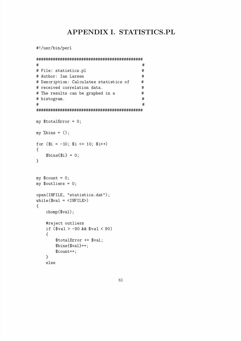
5/12/2018 GetTRDoc - slidepdf.com
http://slidepdf.com/reader/full/gettrdoc-55a35d023bc26 107/116
APPENDIX I. STATISTICS.PL
#!/usr/bin/perl
############################################## #
# File: statistics.pl #
# Author: Ian Larsen #
# Description: Calculates statistics of #
# received correlation data. #
# The results can be graphed in a #
# histogram. #
# #
#############################################
my $totalError = 0;
my %bins = ();
for ($i = -10; $i <= 10; $i++)
$bins$i = 0;
my $count = 0; my $outliers = 0;
open(INFILE, "statistics.dat");
while($val = <INFILE>)
chomp($val);
#reject outliers
if ($val > -90 && $val < 90)
$totalError += $val;$bins$val++;
$count++;
else
81
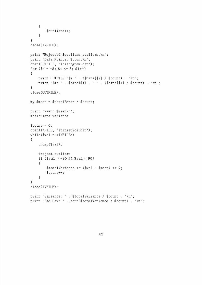
5/12/2018 GetTRDoc - slidepdf.com
http://slidepdf.com/reader/full/gettrdoc-55a35d023bc26 108/116
$outliers++;
close(INFILE);
print "Rejected $outliers outliers.\n";
print "Data Points: $count\n";
open(OUTFILE, ">histogram.dat");
for ($i = -8; $i <= 8; $i++)
print OUTFILE "$i " . ($bins$i / $count) . "\n";
print "$i: " . $bins$i . " " . ($bins$i / $count) . "\n";
close(OUTFILE);
my $mean = $totalError / $count;
print "Mean: $mean\n";
#calculate variance
$count = 0;
open(INFILE, "statistics.dat");
while($val = <INFILE>)
chomp($val);
#reject outliers
if ($val > -90 && $val < 90)
$totalVariance += ($val - $mean) ** 2;
$count++;
close(INFILE);
print "Variance: " . $totalVariance / $count . "\n";
print "Std Dev: " . sqrt($totalVariance / $count) . "\n";
82
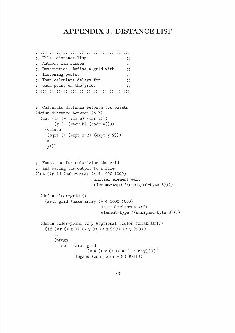
5/12/2018 GetTRDoc - slidepdf.com
http://slidepdf.com/reader/full/gettrdoc-55a35d023bc26 109/116
APPENDIX J. DISTANCE.LISP
;;;;;;;;;;;;;;;;;;;;;;;;;;;;;;;;;;;;;;;;;
;; File: distance.lisp ;;;; Author: Ian Larsen ;;
;; Description: Define a grid with ;;
;; listening posts. ;;
;; Then calculate delays for ;;
;; each point on the grid. ;;
;;;;;;;;;;;;;;;;;;;;;;;;;;;;;;;;;;;;;;;;;
;; Calculate distance between two points
(defun distance-between (a b)
(let ((x (- (car b) (car a)))
(y (- (cadr b) (cadr a))))
(values
(sqrt (+ (expt x 2) (expt y 2)))
x
y)))
;; Functions for colorizing the grid
;; and saving the output to a file
(let ((grid (make-array (* 4 1000 1000):initial-element #xff
:element-type ’(unsigned-byte 8))))
(defun clear-grid ()
(setf grid (make-array (* 4 1000 1000)
:initial-element #xff
:element-type ’(unsigned-byte 8))))
(defun color-point (x y &optional (color #x333333ff))
(if (or (< x 0) (< y 0) (> x 999) (> y 999))
()(progn
(setf (aref grid
(* 4 (+ x (* 1000 (- 999 y)))))
(logand (ash color -24) #xff))
83
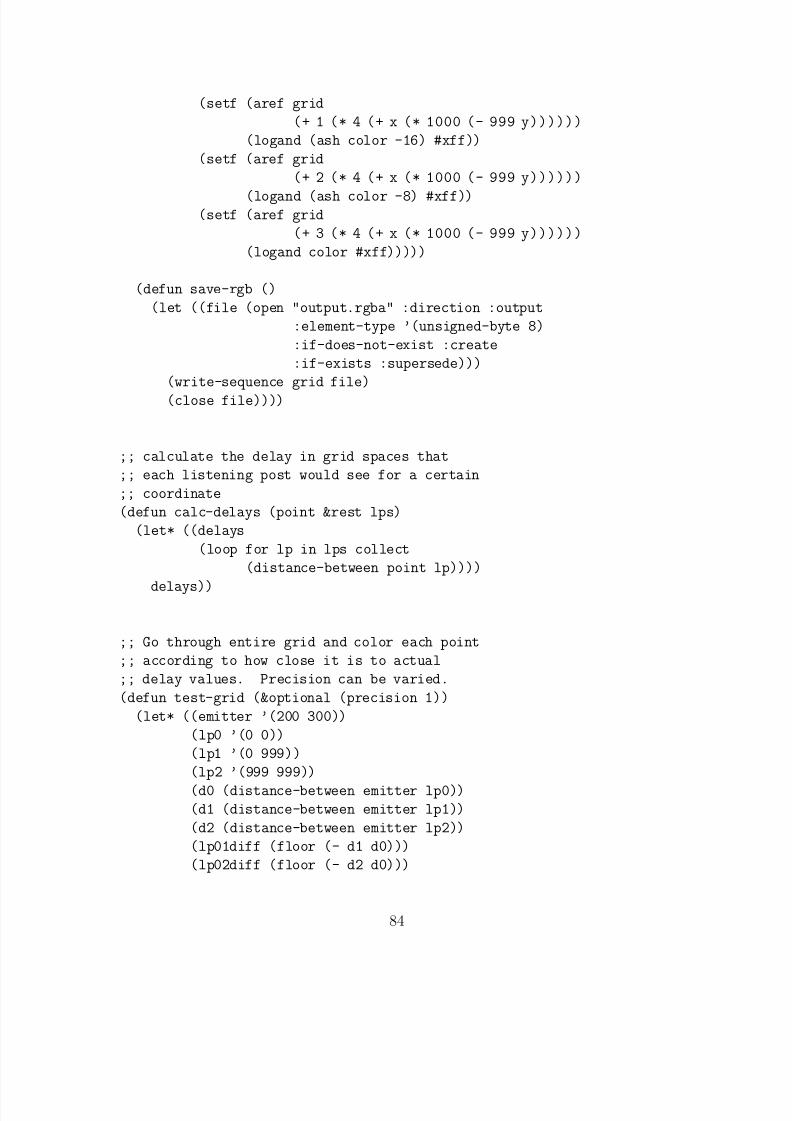
5/12/2018 GetTRDoc - slidepdf.com
http://slidepdf.com/reader/full/gettrdoc-55a35d023bc26 110/116
(setf (aref grid
(+ 1 (* 4 (+ x (* 1000 (- 999 y))))))
(logand (ash color -16) #xff))
(setf (aref grid
(+ 2 (* 4 (+ x (* 1000 (- 999 y))))))
(logand (ash color -8) #xff))(setf (aref grid
(+ 3 (* 4 (+ x (* 1000 (- 999 y))))))
(logand color #xff)))))
(defun save-rgb ()
(let ((file (open "output.rgba" :direction :output
:element-type ’(unsigned-byte 8)
:if-does-not-exist :create
:if-exists :supersede)))
(write-sequence grid file)
(close file))))
;; calculate the delay in grid spaces that
;; each listening post would see for a certain
;; coordinate
(defun calc-delays (point &rest lps)
(let* ((delays
(loop for lp in lps collect
(distance-between point lp))))
delays))
;; Go through entire grid and color each point
;; according to how close it is to actual
;; delay values. Precision can be varied.
(defun test-grid (&optional (precision 1))
(let* ((emitter ’(200 300))
(lp0 ’(0 0))
(lp1 ’(0 999))
(lp2 ’(999 999))
(d0 (distance-between emitter lp0))
(d1 (distance-between emitter lp1))
(d2 (distance-between emitter lp2))
(lp01diff (floor (- d1 d0)))
(lp02diff (floor (- d2 d0)))
84
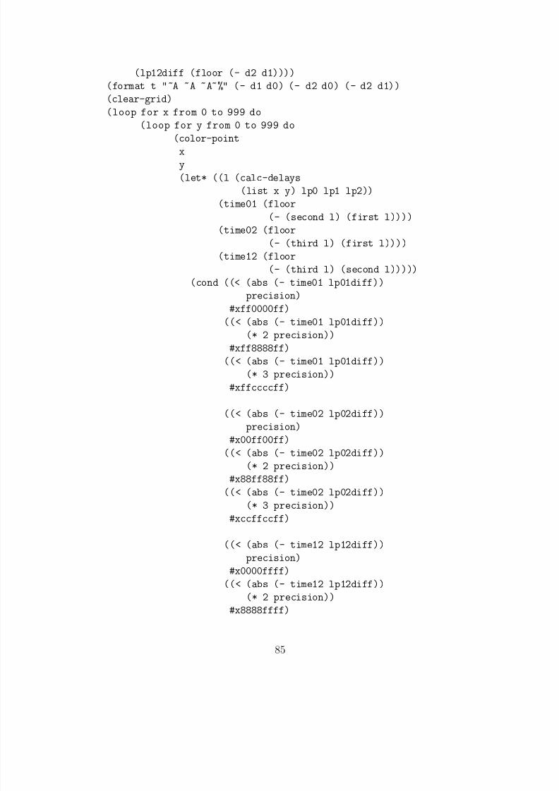
5/12/2018 GetTRDoc - slidepdf.com
http://slidepdf.com/reader/full/gettrdoc-55a35d023bc26 111/116
(lp12diff (floor (- d2 d1))))
(format t "~A ~A ~A~%" (- d1 d0) (- d2 d0) (- d2 d1))
(clear-grid)
(loop for x from 0 to 999 do
(loop for y from 0 to 999 do
(color-pointx
y
(let* ((l (calc-delays
(list x y) lp0 lp1 lp2))
(time01 (floor
(- (second l) (first l))))
(time02 (floor
(- (third l) (first l))))
(time12 (floor
(- (third l) (second l)))))
(cond ((< (abs (- time01 lp01diff))
precision)
#xff0000ff)
((< (abs (- time01 lp01diff))
(* 2 precision))
#xff8888ff)
((< (abs (- time01 lp01diff))
(* 3 precision))
#xffccccff)
((< (abs (- time02 lp02diff))precision)
#x00ff00ff)
((< (abs (- time02 lp02diff))
(* 2 precision))
#x88ff88ff)
((< (abs (- time02 lp02diff))
(* 3 precision))
#xccffccff)
((< (abs (- time12 lp12diff))
precision)
#x0000ffff)
((< (abs (- time12 lp12diff))
(* 2 precision))
#x8888ffff)
85

5/12/2018 GetTRDoc - slidepdf.com
http://slidepdf.com/reader/full/gettrdoc-55a35d023bc26 112/116
((< (abs (- time12 lp12diff))
(* 3 precision))
#xccccffff)
(t
#xffffffff))))))(save-rgb)))
(test-grid 37)
86

5/12/2018 GetTRDoc - slidepdf.com
http://slidepdf.com/reader/full/gettrdoc-55a35d023bc26 113/116
LIST OF REFERENCES
[1] Jeffrey H. Reed. Software Radio: A Modern Approach to Radio Engineering .Prentice Hall, 2002.
[2] David Adamy. EW101: A First Course in Electronic Warfare. Artech House,2001.
[3] Upendra Ramdat. Software Communications Architecture (SCA) compliant soft-ware radio design for Interim Standard 95B (IS-95B) transceiver. Master’s thesis,Naval Postgraduate School, 2007.
[4] Kian Wai Low. Software Communications Architecture (SCA) compliant soft-ware defined radio design for IEEE 802.16 wirelessman-OFDMTMtransceiver.Master’s thesis, Naval Postgraduate School, 2006.
[5] Wai Kiat Chris Leong. Software defined radio design for an IEEE 802.11Atransceiver using open source Software Communications Architecture (SCA) im-plementation::embedded (OSSIE). Master’s thesis, Naval Postgraduate School,2006.
[6] Glenn D. Hartwell. Improved geo-spatial resolution using a modified approachto the complex ambiguity function (CAF). Master’s thesis, Naval PostgraduateSchool, 2005.
[7] Juan Sanfuentes. Software Defined Radio Design for Synchronization of 802.11aReceiver. Master’s thesis, Naval Postgraduate School, 2007.
[8] Juan P. Svenningsen. Modeling, simulation and implementation of a non-coherent binary-frequency-shift-keying (BFSK) receiver-transmitter into a fieldprogrammable gate array (FPGA). Master’s thesis, Naval Postgraduate School,2005.
[9] Michel Mouly and Marie-Bernadette Pautet. The GSM System for Mobile Com-munications. Cell & Sys, 1992.
[10] 3rd Generation Partnership Project; Technical Specification Group GSM/EDGE.3GPP TS 45.002: Radio Access Network; Multiplexing and multiple access on the radio path (Release 7), 2007.
[11] Gunnar Heine. GSM Networks: Protocols, Terminology, and Implementation .Artech House, 1998.
[12] 3rd Generation Partnership Project; Technical Specification Group GSM/EDGE.3GPP TS 45.004: Radio Access Network; Modulation (Release 6), 2005.
87
5/12/2018 GetTRDoc - slidepdf.com
http://slidepdf.com/reader/full/gettrdoc-55a35d023bc26 114/116
[13] Theodore S. Rappaport. Wireless Communications: Principles and Practice2ndEdition. Prentice Hall, 2002.
[14] Dawei Shen. Tutorial 4: The USRP Board . http://www.nd.edu/∼jnl/sdr/
docs/tutorials/4.html. (Accessed September 2007).
[15] Roberto Christi. Modern Digital Signal Processing . Brooks/Cole, 2004.
[16] GNU Radio 3.0 Documentation: usrp standard tx Class Reference.http://gnuradio.org/doc/doxygen/classusrp standard tx.html. (Ac-cessed September 2007).
[17] John G. Proakis. Digital Communications. McGraw Hill, 2001.
[18] Alan V. Oppenheim and Alan S. Willsky. Signals and Systems. Prentice Hall,1983.
[19] Vladimir Vassilevsky. FM Demodulation. http://www.dsprelated.com/showmessage/67382/1.php. (Accessed September 2007).
88
5/12/2018 GetTRDoc - slidepdf.com
http://slidepdf.com/reader/full/gettrdoc-55a35d023bc26 115/116
INITIAL DISTRIBUTION LIST
1. Defense Technical Information CenterFt. Belvoir, VA
2. Dudley Knox LibraryNaval Postgraduate SchoolMonterey, CA
3. Ian LarsenNaval Postgraduate SchoolMonterey, CA
4. Frank KraghNaval Postgraduate SchoolMonterey, CA
5. Clark RobertsonNaval Postgraduate SchoolMonterey, CA
6. Donna MillerNaval Postgraduate SchoolMonterey, CA
7. Roberto CristiNaval Postgraduate School
Monterey, CA
8. Tri HaNaval Postgraduate SchoolMonterey, CA
9. Herschel LoomisNaval Postgraduate SchoolMonterey, CA
10. Peter AteshianNaval Postgraduate SchoolMonterey, CA
11. Giovanna OritiNaval Postgraduate SchoolMonterey, CA
89
5/12/2018 GetTRDoc - slidepdf.com
http://slidepdf.com/reader/full/gettrdoc-55a35d023bc26 116/116
12. Alex JulianNaval Postgraduate SchoolMonterey, CA
13. Alan Ross
Naval Postgraduate SchoolMonterey, CA
14. Tim MeehanNaval Postgraduate SchoolMonterey, CA
15. Nathan BeltzNaval Postgraduate SchoolMonterey, CA
16. Ray Cole
U.S. Naval Research LaboratoryWashington, DC
17. Rich NorthJTRSJPEOSan Diego, CA
18. Gerry BaumgartnerSPAWARSan Diego, CA
90