Embed Size (px)
Citation preview

NONDESTRUCTIVE EVALUATION OF AIRCRAFT
COMPOSITES USING TERAHERTZ TIME DOMAIN SPECTROSCOPY
DISSERTATION
Christopher D. Stoik, Lieutenant Colonel, USAF AFIT/DS/ENP/09-D02
DEPARTMENT OF THE AIR FORCE AIR UNIVERSITY
AIR FORCE INSTITUTE OF TECHNOLOGY
Wright-Patterson Air Force Base, Ohio
APPROVED FOR PUBLIC RELEASE; DISTRIBUTION UNLIMITED

The views expressed in this dissertation are those of the author and do not reflect the official policy or position of the United States Air Force, Department of Defense, or the United States Government.

AFIT/DS/ENP/09-D02
NONDESTRUCTIVE EVALUATION OF AIRCRAFT COMPOSITES
USING TERAHERTZ TIME DOMAIN SPECTROSCOPY
DISSERTATION
Presented to the Faculty
Graduate School of Engineering and Management
Air Force Institute of Technology
Air University
Air Education and Training Command
In Partial Fulfillment of the Requirements for the
Degree of Doctor of Philosophy
Christopher D. Stoik, BS, MS
Lieutenant Colonel, USAF
December 2008
APPROVED FOR PUBLIC RELEASE; DISTRIBUTION UNLIMITED


iv
AFIT/DS/ENP/09-D02
Abstract
Terahertz (THz) time domain spectroscopy (TDS) was assessed as a
nondestructive evaluation technique for aircraft composites. Material properties of glass
fiber composite were measured using both transmission and reflection configuration. The
interaction of THz with a glass fiber composite was then analyzed, including the effects
of scattering, absorption, and the index of refraction, as well as effective medium
approximations. THz TDS, in both transmission and reflection configuration, was used
to study composite damage, including voids, delaminations, mechanical damage, and heat
damage. Measurement of the material properties on samples with localized heat damage
showed that burning did not change the refractive index or absorption coefficient
noticeably; however, material blistering was detected. Voids were located by THz TDS
transmission and reflection imaging using amplitude and phase techniques. The depth of
delaminations was measured via the timing of Fabry-Perot reflections after the main
pulse. Evidence of bending stress damage and simulated hidden cracks was also detected
with terahertz imaging.
v
Acknowledgements
First, I would like to thank my advisor, Lt Col Matt Bohn, for his guidance in this
research, offering skillful advice with the laboratory experimental setup and providing
expert scientific insight in helping me to resolve research issues. I would also like to
thank Dr. Jim Blackshire of AFRL/RXLP for sponsoring this work and for providing us
with representative aircraft composite samples which were essential to the research. In
addition, I would like to thank Abel Nunez for his help with image processing and to
Jeremy Johnson and AFRL/RXLP for the ultrasound and x-ray images. Thanks to Col
Brent Richert and my parents for their encouragement to return to school and earn this
degree and to my mother for helping to proofread this dissertation.
I would like to thank Epiphany Lutheran Church for its spiritual support along the
way. I am very grateful for the birth of my two children who have been an inspiration to
me and represent promise for the future. Most of all, I would like to thank my wife for
her patience and understanding during the difficult days and nights when I was studying,
researching, and writing. I also thank her for her strength in enduring an uncomfortable
work situation for 4 years.

vi
Table of Contents Abstract ......................................................................................................................................... iv Acknowledgements ..................................................................................................................... v List of Figures ............................................................................................................................. ix List of Tables ............................................................................................................................. xiv
1. Introduction .................................................................................................................... 1
1.1 Background ............................................................................................................. 2 1.2 Problem Statement .................................................................................................. 3 1.3 Research Objectives ................................................................................................ 4 1.4 Experimental Approach .......................................................................................... 5 1.5 Assumptions/ Limitations ....................................................................................... 5 1.6 Overview ................................................................................................................. 6
2. Theory and Background ................................................................................................. 8
2.1 THz Pulse Generation ............................................................................................. 8 2.1.1 Photoconductive Antennas.......................................................................... 9 2.1.2 Optical Rectification in Nonlinear Media ................................................. 11
2.2 THz Pulse Detection ............................................................................................. 13 2.2.1 Photoconductive Antennas........................................................................ 13 2.2.2 Electro-Optic Sampling in Crystals .......................................................... 14
2.3 Terahertz Time Domain Spectroscopy System ..................................................... 16 2.3.1 Femtosecond Laser ................................................................................... 18 2.3.2 THz Beam Optics ...................................................................................... 18
2.3.2.1 Substrate Lens ............................................................................ 19 2.3.2.2 Off-Axis Parabolic Mirrors ........................................................ 20 2.3.2.3 Gaussian Beams .......................................................................... 20 2.3.2.4 Gaussian Beam Expansion ......................................................... 22
2.3.3 Scanning Optical Delay Line .................................................................... 23 2.3.4 Raster Scanner .......................................................................................... 23 2.3.5 Lock-in Amplifier ..................................................................................... 24
2.4 THz TDS Data Analysis on Composites .............................................................. 25 2.4.1 Material Parameter Estimation ................................................................. 27 2.4.2 Drude Model ............................................................................................. 28 2.4.3 Scattering .................................................................................................. 29 2.4.4 Effective Medium Approximations .......................................................... 34 2.4.5 Imaging ..................................................................................................... 35 2.4.6 Image Processing ...................................................................................... 37
2.5 THz TDS Literature Review ................................................................................. 39

vii
2.5.1 Composites ................................................................................................ 39 2.5.2 Ceramics ................................................................................................... 41 2.5.3 Paint Thickness over Metallic Surfaces .................................................... 42 2.5.4 Semiconductors ......................................................................................... 43 2.5.5 Measuring Material Properties with THz Radiation ................................. 44
2.5.5.1 Transmission Mode Measurement Technique ............................ 44 2.5.5.2 Literature Summary of THz Material Parameter Measurements 47
2.5.6 THz TDS for NDE .................................................................................... 49
3. Material Parameter Estimation with Terahertz TDS .................................................... 51
3.1 THz TDS System Characterization ....................................................................... 51 3.1.1 THz TDS Output Specifications ............................................................... 52 3.1.2 Water Vapor Absorption Spectra .............................................................. 54 3.1.3 THz Pulse and Spectrum Modeling .......................................................... 55 3.1.4 System Setup Challenges .......................................................................... 58
3.2 Transmission Mode Measurements ...................................................................... 59 3.2.1 Calculation Technique .............................................................................. 60 3.2.2 Measurement Results on Various Materials ............................................. 62 3.2.3 Effective Medium Approximation and Scattering Analysis ..................... 66 3.2.4 Material Parameter Calibration ................................................................. 71
3.2.4.1 Drude Model Predictions ............................................................ 71 3.2.4.2 Silicon Measurements ................................................................ 73
3.2.5 Fabry-Perot Resonance Removal Techniques .......................................... 75 3.3 Reflection Mode Material Parameter Measurements ........................................... 79
3.3.1 Calculation Technique .............................................................................. 80 3.3.2 Practical Approximation of Material Parameters ..................................... 82 3.3.3 Other Material Parameter Measurements ................................................. 84
3.4 Burn Diagnostics Using THz TDS ....................................................................... 87 3.4.1 Transmission Mode ................................................................................... 88 3.4.2 Reflection Mode........................................................................................ 90
4. THz Imaging for Nondestructive Evaluation ............................................................... 92
4.1 Sample Preparation ............................................................................................... 92 4.2 Transmission Mode Setup..................................................................................... 93 4.3 THz Beam Propagation and Modeling ................................................................. 94
4.3.1 Spot Size Minimization............................................................................. 95 4.3.2 THz Beam Measurements ......................................................................... 97
4.4 Imaging of Composites with Transmission Setup ................................................ 99 4.4.1 THz TDS Thickness Measurements ......................................................... 99 4.4.2 Image Processing Comparison ................................................................ 100 4.4.3 2-D Imaging Results ............................................................................... 102
4.4.3.1 Imaging of Burn Damage ......................................................... 104 4.4.3.2 Imaging of Bending Damage .................................................... 108 4.4.3.3 Imaging of Hidden Defects ...................................................... 109

viii
4.4.4 Depth of Delamination Analysis ............................................................. 110 4.5 Reflection Mode Imaging of Composites ........................................................... 113
4.5.1 Thickness Calibration ............................................................................. 113 4.5.2 2-D Imaging Results ............................................................................... 114
4.5.2.1 Imaging of Burn Damage ......................................................... 115 4.5.2.2 Imaging of Bending Damage .................................................... 118 4.5.2.3 Imaging of Hidden Defects ...................................................... 118 4.5.2.4 Imaging and Analysis of Entire Panels .................................... 119 4.5.2.5 Paint Thickness Approximations .............................................. 122
4.5.3 Depth of Delaminations Analysis ........................................................... 123
5. Conclusions and Recommendations .......................................................................... 128
5.1 Major Research Contributions ............................................................................ 128 5.2 Conclusions ......................................................................................................... 128 5.3 Future Work ........................................................................................................ 132
Bibliography ............................................................................................................................. 137 Vita ............................................................................................................................................ 145
ix
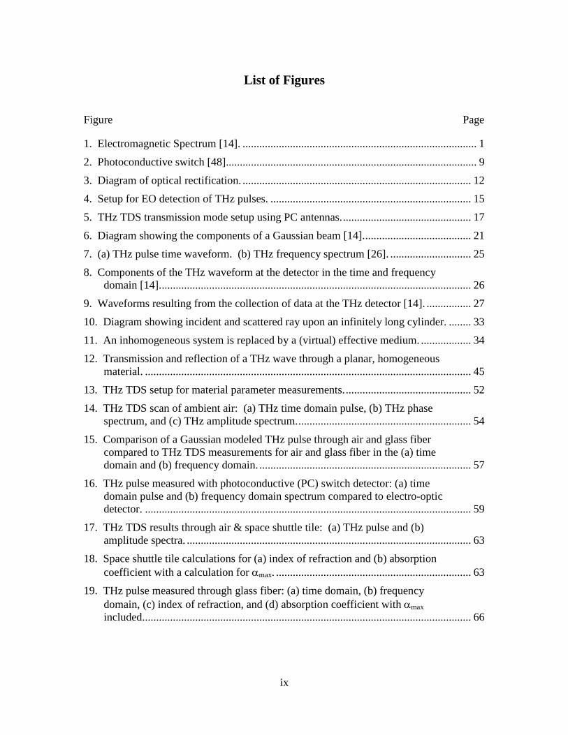
List of Figures
Figure Page
1. Electromagnetic Spectrum [14]. .................................................................................... 1
2. Photoconductive switch [48]. ......................................................................................... 9
3. Diagram of optical rectification. .................................................................................. 12
4. Setup for EO detection of THz pulses. ........................................................................ 15
5. THz TDS transmission mode setup using PC antennas. .............................................. 17
6. Diagram showing the components of a Gaussian beam [14]. ...................................... 21
7. (a) THz pulse time waveform. (b) THz frequency spectrum [26]. ............................. 25
8. Components of the THz waveform at the detector in the time and frequency domain [14]. ............................................................................................................... 26
9. Waveforms resulting from the collection of data at the THz detector [14]. ................ 27
10. Diagram showing incident and scattered ray upon an infinitely long cylinder. ........ 33
11. An inhomogeneous system is replaced by a (virtual) effective medium. .................. 34
12. Transmission and reflection of a THz wave through a planar, homogeneous material. ..................................................................................................................... 45
13. THz TDS setup for material parameter measurements. ............................................. 52
14. THz TDS scan of ambient air: (a) THz time domain pulse, (b) THz phase spectrum, and (c) THz amplitude spectrum. .............................................................. 54
15. Comparison of a Gaussian modeled THz pulse through air and glass fiber compared to THz TDS measurements for air and glass fiber in the (a) time domain and (b) frequency domain. ............................................................................ 57
16. THz pulse measured with photoconductive (PC) switch detector: (a) time domain pulse and (b) frequency domain spectrum compared to electro-optic detector. ..................................................................................................................... 59
17. THz TDS results through air & space shuttle tile: (a) THz pulse and (b) amplitude spectra. ...................................................................................................... 63
18. Space shuttle tile calculations for (a) index of refraction and (b) absorption coefficient with a calculation for αmax. ...................................................................... 63
19. THz pulse measured through glass fiber: (a) time domain, (b) frequency domain, (c) index of refraction, and (d) absorption coefficient with αmax included. ..................................................................................................................... 66

x
20. THz TDS material parameter measurements using actual thickness measurements from polyimide showing (a) index of refraction and (b) absorption coefficient. ............................................................................................... 67
21. Scattering coefficient calculation for glass fiber in the THz frequency range. ......... 69
22. (a) Extinction coefficient estimation on glass weave assuming an air-glass index mixture. (b) Comparison of the Bruggeman EMA for glass fiber extinction using polyimide and glass weave data vs. actual glass fiber extinction data. (c) Scattering coefficient calculations for the air and glass weave mixture. (d) Comparison of EMA for glass fiber using polyimide and glass weave (scattering removed) vs. glass fiber extinction coefficient. ................... 70
23. Material parameter measurements on a silicon wafer: (a) THz pulse showing FP reflections, (b) THz spectrum, (c) index of refraction, and (d) absorption coefficient. ................................................................................................................. 73
24. Material parameter measurements on high resistivity silicon: (a) THz pulse, (b) THz spectrum, (c) index of refraction, and (d) absorption coefficient. ............... 74
25. Material parameter measurements on 6 mm thick float zone (FZ) silicon: (a) THz pulse, (b) THz spectrum, (c) index of refraction, and (d) absorption coefficient. ................................................................................................................. 75
26. Diagrams showing the removal of FP oscillations in the time domain: (a) index of refraction with FP oscillations, (b) index of refraction without first 2 FP oscillations, (c) absorption coefficient with FP oscillations, (d) absorption without first 2 FP oscillations. ................................................................................... 77
27. Iterative process for removal Fabry-Perot etalon effect in frequency domain described by Duvillaret et. al. .................................................................................... 77
28. Fabry-Perot oscillation removal technique showing the real part of the index of refraction (a) before & (b) removal, followed by the imaginary part of the index of refraction (c) before & (d) after the Fabry-Perot removal technique was applied. ............................................................................................................... 78
29. THz TDS reflection mode schematic. ........................................................................ 79
30. Material parameter measurements using reflection configuration on 6 mm thick float zone (FZ) silicon: (a) index of refraction and (b) absorption coefficient. ................................................................................................................. 82
31. THz TDS reflection setup for thick FZ silicon: (a) pulses off front and back surface and (b) absorption coefficient using Fourier transform from each pulse. .......................................................................................................................... 83
32. Diagram showing the geometry of the first Fabry-Perot reflection from the sample in reflection configuration. ............................................................................ 84
33. THz TDS reflection (a) pulse and (b) spectrum for 1.016 mm high resistivity silicon. Isolation of the (c) front reflected pulse and the (d) back side

xi
reflected pulse in the time domain. The (e) absorption coefficient for high resistivity silicon measured using the spectrum of the front and back pulse. ............ 85
34. Plot of the (a) THz pulses reflected from the front and back of a glass fiber coupon. Absorption coefficient for the glass fiber (b) without filtering and (c) with filtering. ........................................................................................................ 87
35. THz TDS (a) pulse and (b) amplitude spectra for air reference and coated glass fiber. (c) Index of refraction and (d) absorption coefficient measurements for coated glass fiber in the THz frequency range. ............................ 88
36. THz TDS material parameter measurements using actual thickness measurements for burn damage areas showing (a) indices of refraction and (b) absorption coefficients. ........................................................................................ 89
37. THz TDS material parameter measurements, assuming the same thickness, for burn damage areas showing (a) indices of refraction and (b) absorption coefficients. ................................................................................................................ 90
38. Comparison of the reflected signal from a coated and uncoated sample, showing the (a) time domain and (b) frequency spectrum returns. ........................... 91
39. Photograph showing the 5 glass fiber samples: (1) thickness calibration sample, (2) & (3) burn samples, (4) mechanical stress sample, and (5) hidden defect sample showing the hidden location of two of the eight defects. ................... 93
40. THz TDS Setup for Imaging Composites in Transmission Mode. ............................ 94
41. Diagram showing the transmission optical system with THz beam focusing on sample at 1 THz. ................................................................................................... 96
42. Diagram showing the reflection optical system with THz beam focusing on sample at 1 THz. ........................................................................................................ 97
43. Diagram showing the geometry of the incident and reflected beam off the apparatus for measuring the THz spot size in TDS reflection configuration. ........... 99
44. Relative delay of THz pulses for various thicknesses of glass fiber sample, including those that were etched (*). ....................................................................... 100
45. THz image of a 12.5 mm diameter circle etched in glass fiber showing (a) the original 1X1 mm pixel image, (b) image after MATLAB ‘interp’ function, (c) image after zero-padding 10 times in the spatial frequency domain, and (d) final image after applying MATLAB ‘interp’ function to part (c). (e) Comparison of (c) with 1/10th scale pixel image. .................................................... 101
46. Image comparison showing the (a) the zero-padding technique (10 times) and the (b) zero-padding technique (4 times) with the addition of a Wiener filter. ....... 102
47. THz TDS transmission images showing a section of the glass fiber that had been milled to two different thicknesses using peak pulse amplitude (a) and peak pulse position (b) techniques. A picture of the scan area on the calibration sample (c). ............................................................................................. 103

xii
48. THz images formed by summing the area under the curve of the amplitude spectrum within a given frequency range for each pixel: (a) 0.1 – 1.3 THz, (b) 0.5 – 0.7 THz, (c) 0.7 – 0.9 THz. ....................................................................... 104
49. THz TDS images and photos for three burn areas on glass fiber samples: (a), (d) 440°C for 4 minutes; (b), (e) 430°C for 6 minutes; and (c), (f) 425°C for 20 minutes. ............................................................................................................... 105
50. THz TDS (a) pulse image and (b) amplitude spectra for undamaged glass fiber sample and for an area with burn damage (440°C for 4 minutes). (c) THz TDS amplitude image of high resistivity silicon. ............................................ 106
51. THz TDS image showing bend damage across the central bend axis (a). Photographs of the (b) front side of the composite strip showing the scan area with the location of the taped ‘X’ and the (c) back side showing the location of the cracking and buckling and the hexagonal structure. (d) Ultrasound image of the bend damage. ...................................................................................... 108
52. THz TDS images showing 3 mm diameter milled area hidden between two glass fiber strips using (a) peak pulse amplitude and (b) peak pulse position. Linear slit void (6 mm length) (c) also hidden between two strips of glass fiber. The final picture is an x-ray computed tomography scan of the laminated sample showing the hidden circular and slit voids in the sample. .......... 109
53. THz pulses after propagating through (a) laminated and delaminated portions of a glass fiber strip. (b) Autocorrelation of each of the two pulses showing the approximate location of Fabry-Perot reflections. Thz pulse propagation in the opposite direction showing pulses and their autocorrelations (c), (d). .......... 111
54. (a) Diagram showing the main pulse and the first Fabry-Perot reflection in transmission configuration. (b) A chart showing the relative amplitude of the first Fabry-Perot reflection to the main pulse after traveling through various thicknesses of composite. (c) A photograph showing the delamination. ............... 112
55. THz TDS reflection images showing a section of the glass fiber that had been milled to two different thicknesses using peak pulse amplitude (a) and peak pulse position (b) techniques. The final image (c) shows a thickness estimation for a separate scan. ................................................................................. 114
56. THz TDS reflection images for burn damage from heating at 440°C for 4 minutes for (a) peak pulse amplitude and (b) peak pulse position. Pulse return from the right side of the bubble showing the double pulse return (c). X-ray computed tomography image showing a side profile of the large burn blister (d). ................................................................................................................. 116
57. THz TDS reflection images showing the (a) minimum peak amplitude for burning at 430°C for 6 minutes and the (b) peak pulse amplitude for burning at 425°C for 20 minutes. .......................................................................................... 117
58. THz TDS reflection image using the amplitude of frequencies (1.2 – 1.4 THz) showing bend damage across the central bend axis. ................................................ 118

xiii
59. THz TDS reflection image showing 3 mm diameter milled area hidden between two glass fiber strips using the amplitude of the Fabry-Perot reflection from the void. .......................................................................................... 119
60. THz TDS reflection setup scan on entire panel with puncture hole (4.5 mm diameter) and two burn blisters. Images were constructed using the (a) minimum peak pulse amplitude, (b) maximum peak pulse position, and (c) the frequency spectrum amplitude added under the curve (1.4 – 1.6 THz). THz pulses reflected from coated surface and partially uncoated burn blister (d). ............................................................................................................................ 120
61. THz images constructed using the (a) peak pulse amplitude and (b) peak pulse position of a panel with its coating dissolved away by butanone. ................. 121
62. THz TDS (a) time domain plots and (b) frequency spectra for a coated and uncoated surface of an aircraft panel. ...................................................................... 122
63. THz TDS reflection configuration plots showing the (a) time domain pulse with a double peak and the (b) THz amplitude spectrum. ....................................... 123
64. (a) Diagram of a delaminated sample showing the first Fabry-Perot reflection in reflection configuration. (b) A chart showing the relative strength of the first Fabry-Perot reflection after traveling through various thicknesses of glass fiber composite before the delamination. (c) A chart showing the relative strength of the first Fabry-Perot reflection from discontinuities including both glue-glass fiber (G-GF) and air-glass fiber (A-GF). ....................... 124
65. THz TDS time domain plots showing reflections from discontinuities: (a) air and (b) adhesive. ...................................................................................................... 125
66. Fourier deconvolution of the discontinuities present in a glass fiber sample laminated at various thicknesses: (a) 0.23 mm, (b) 0.46 mm, (c) 0.69 mm, (d) 0.92 mm, (e) 0.92 mm delaminated, and (f) no lamination. Fourier deconvolution with the TDS system characteristics subtracted are shown next. The various thicknesses were measured in the opposite direction: (g) 0.23 mm, (h) 0.23 mm delaminated, (i) 0.46 mm, (j) 0.69 mm, (k) 0.92 mm, and (l) no lamination. ............................................................................................... 126
67. Comparison of the calculated time for F-P reflections through glass fiber to the measured autocorrelation values measured in both transmission and reflection configuration. .......................................................................................... 127
68. Summary charts showing the relative amplitude of the first Fabry-Perot reflection to the main pulse after traveling through various thicknesses of glass fiber composite in (a) transmission configuration and (b) reflection configuration. ........................................................................................................... 132
69. Comparison of various types of glass fiber damage/alterations between transmission and reflection configuration. .............................................................. 133

xiv
List of Tables
Table Page
1. THz Time Domain Spectrometer specifications and measurements. .......................... 53
2. Absorption spectrum rotational transitions for water vapor between 0.2 – 2.4 THz [82]. .................................................................................................................... 55
3. List of Specifications for Ekspla photoconductive switch components. ...................... 58
4. Sources of error for THz material parameter measurements. ...................................... 62
5. Summary of results for effective medium approximations on space shuttle tile at 0.5 THz. ................................................................................................................. 64
6. Drude Model parameters and predictions for Silicon at 1 THz. .................................. 72
7. Ekspla measurements at the exit of the silicon hemispherical lens. ............................ 95
8. Comparison of diffraction-limited spot sizes with THz beam optical design focus spot sizes for the transmission configuration. .................................................. 96
9. Comparison of diffraction-limited spot sizes with THz beam optical design focus spot sizes for the reflection configuration. ....................................................... 97

1
Nondestructive Evaluation of Aircraft Composites Using
Terahertz Time Domain Spectroscopy
1. Introduction
Terahertz (THz) radiation can be defined as the region of the electromagnetic
spectrum with frequencies between 0.1 THz and 10 THz or with wavelengths between 3
mm and 30 μm. The THz “gap”, as shown in Figure 1, falls between the microwave
region and the infrared/optical region. Microwave electronic devices are typically
comparable in size to the wavelength of the radiation and support single-mode or low-
order mode guided waves. In contrast, optical and infrared devices have dimensions
much larger than a wavelength and often support beams containing many modes. The
merging of laser and optics technology with micro chip electronics technology has been
instrumental in the development of THz devices and the advancement of THz research.
Figure 1. Electromagnetic Spectrum [14].
106 107 108 109 1010 1011 1012 1013 1014 1015 1016
Radio Microwave THz IR UV
103 102 101 100 10-1 10-2 10-3 10-4 10-5 10-6 10-7
Frequency (Hz)
Wavelength (m)
Visible

2
1.1 Background
With the rapid advances in the development of laser technology, nonlinear optics
and optoelectronic techniques for the production and measurement of terahertz radiation
have proliferated. One of the earliest and most promising of these techniques is
terahertz time-domain spectroscopy (THz TDS), a method which relies on the generation
of broadband electromagnetic transients using ultrafast laser pulses. Several novel
measurement capabilities have become practical, including time-resolved techniques like
the optical pump – THz probe measurement, THz emission spectroscopy, and THz
correlation spectroscopy. The first reported use of THz TDS for imaging was reported in
1995 and this work has sparked a flood of interest and suggested a range of new
applications for THz “T-ray” imaging [48]. It has even received media attention recently
in the novel Games of State, by Tom Clancy [15].
Composite materials such as fiberglass, Kevlar, and carbon fiber have high
strength to weight ratios and are increasingly being used as structural components in high
performance military aircraft [89]. The navy’s F/A-18A/B and the F/A-18E/F structural
weights are composed of 10% and 19% composites, and approximately 24% of the F-
22’s structural weight is composite in origin. The F-35 Joint Strike Fighter will also have
a high percentage of its weight made up of composites.
Fiber composites not only impart increased strength to aircraft structures, but also
improve aerodynamic performance, increase safety, and reduce corrosion. However,
composites can be weakened by various defects that are created during either fabrication
or during the lifecycle of the aircraft. In the layer build-up stage of the manufacturing
process, foreign debris can become embedded within the composite layers, and voids can

3
be formed by air bubbles or large gaps between the fiber weave. Defects that are caused
by foreign debris or voids decrease the layer adhesion and the overall strength of a
composite component. Current quality control methods are incapable of finding these
defects until curing has been completed, requiring that the component be reworked or
thrown out and increasing the cost of part production. Additionally, routine maintenance
of in-service composite materials requires the application of relatively complex
inspection and repair techniques, which often have to be performed in the field.
New techniques are being explored to improve the efficiency of composite part
inspection during construction and repair. THz radiation offers potential efficiency
improvements, because it has the unique ability to penetrate composites and identify
foreign debris and other defects such as delaminations, air bubbles, and heat damage.
THz would offer a non-invasive, non-contact, non-ionizing way of assessing composite
part condition and could help overcome the shortcomings of other nondestructive
evaluation (NDE) techniques such as x-rays, ultrasound, video inspection, eddy currents,
and thermographic techniques.
1.2 Problem Statement
Significant progress has been made recently in the development of the sources
and technology for THz imaging, sensing, and spectroscopic and communications
applications, but the technology still remains limited compared to that used for the
microwave and optical regions of the spectrum. THz technology is being used in an
increasingly wide variety of applications including: information and communications
technology; biology and medical sciences; homeland security; quality control of food and

4
agricultural products; global environment monitoring; ultrafast computing; and NDE
among others. Effective NDE can be performed with a THz imaging system; however, a
THz imaging system demands a high repetition scan rate and a high average power for
favorable signal-to-noise ratios. To fully take advantage of this emerging technology will
require more compact, efficient, and higher power sources. This research effort attempts
to take advantage of commercially available THz sources in an effort to more effectively
characterize and image composite materials.
Innovative solutions for quality control of composite materials during the
manufacturing process and subsequent routine maintenance are needed by the Air Force
to save time and lower cost. As a NDE technique, THz imaging has the potential to be an
effective method of quality control and maintenance inspection of composites. Although
techniques have been developed to measure material properties at THz frequencies, work
still needs to be done to understand and characterize the electromagnetic interaction of
THz with various materials. The optical and electrical properties of composites need to
be fundamentally understood to improve imaging techniques for NDE. Additionally, the
capability of THz TDS in both transmission and reflection configuration should be tested
on representative damage samples for effectiveness.
1.3 Research Objectives
The objective of this dissertation is to evaluate THz TDS for nondestructive
testing and evaluation of aircraft composites by using theory, modeling, and
experimentation to analyze the interaction of THz radiation with composite materials.
An additional objective is to show that THz imaging shows promise for NDE, especially

5
when imaged with a high average power, high repetition rate source and a fast scanning
and collection technique for inspecting the sample.
1.4 Experimental Approach
The first step of this research was to set up a THz TDS system in transmission
configuration using a photoconductive switch for the transmitter and an electro-optic
crystal for the receiver. Using this setup initially, data was collected to make estimates of
optical and electrical parameters for semiconductors and various composite materials,
such as space shuttle foam insulation and aircraft glass fiber composites. The composite
material parameters could then be used, along with effective medium theory and
scattering theory, to describe the interaction of the THz radiation with the sample. Then
a series of THz images, formed with a raster scan pattern, and depth measurements were
collected on samples prepared with various forms of representative damage.
The next step in the experiment was to change the THz TDS system to a
reflection configuration. With this setup, the material parameter measurements were
measured on the same samples used in the transmission experiments. Finally, reflection
mode images and depth measurements were taken on the same damage samples for a
comparison of the two scan methods.
1.5 Assumptions/ Limitations
The variety of aircraft composite samples available for this research was
somewhat limited, but encompassed a representative set of damages that aircraft
composites could encounter. Additionally, the ability to obtain the limited set of

6
representative aircraft damage samples allowed this research to be unique and interesting.
The research was restricted to glass fiber composites, however, because of the inability of
THz radiation to penetrate other composites like carbon fiber. It was also difficult and
expensive to obtain semiconductor samples with low resistivities, due to the
manufacturers’ reluctance to sell wafers in small quantities. The assumption was made
that a high resistivity wafer was sufficient to calibrate a THz TDS system. Another of
our limitations was that we had limited knowledge about the properties, structure, and
volume concentration of the composite constituents. This resulted in making
assumptions for the effective medium and scattering approximations.
The lab setup that was used was limited in its ability to collect THz TDS data at a
fast enough rate to be considered operationally useful. The assumption was made that the
data we collected to make material parameter measurements and to form images was for
a proof of concept demonstration and that other organizations are developing the means
to rapidly scan large samples in short amounts of time. Commercially available THz,
optical, and mechanical components were sufficient to conduct this research, but
customized components and techniques could allow the THz beam to be more tightly
focused onto the sample and scanned at a faster rate to maximize defect detection.
1.6 Overview
The following chapters of this dissertation outline the theory, literature review,
experimental setups, data collection and analysis, and imaging of composite materials
with THz TDS in various configurations. Chapter 2 begins by describing the theory for
the emitter and detector technology used in this research, followed by a description of the

7
components of the THz TDS system. The next section describes data analysis, including
material parameter estimation, scattering, and imaging. The chapter closes with a
summary of some of the recent findings in the literature regarding the use of THz for
NDE.
Chapter 3 describes the data collection, analysis, and results of the material
parameter estimation of the composite materials studied in this dissertation. The first
section explains the setup and characterization of the THz TDS data collection system.
This is followed by the analysis of material parameters collected using the transmission
mode, including a comparison with the Drude Model, Fabry-Perot cancellation
techniques, and effective medium and scattering approximations. The next section is
dedicated to making the same material parameter calculations using THz TDS in
reflective mode. The last section concludes with an analysis of THz TDS material
parameter measurements on burn damage as a potential NDE technique.
In chapter 4, the imaging and analysis of composite damage is the focus, using
both transmission and reflection configurations. The first section explains the
optimization of the THz optical system design for a minimized spot size and the image
processing technique used during post processing. The next section shows the results of
transmission mode imaging of the damage samples and a depth of delamination analysis.
The last section of chapter 4 shows the results of 2-D imaging and depth analysis on the
same samples using the reflection setup. The last chapter shows a summary of the results
and recommendations for future THz research.

8
2. Theory and Background
In order to estimate the optical and electrical parameters of a material using THz
TDS or image that material using THz TDS, it is necessary to establish the theoretical
background on the generation and detection of THz radiation as well as measurement
techniques. This chapter lays the foundation required to explore the properties of
composite materials at THz frequencies and the insight to investigate THz TDS as a NDE
technique.
2.1 THz Pulse Generation
In recent years scientists have developed numerous techniques for generating THz
radiation in an effort to explore this spectral region. This research dealt solely with
pulsed THz sources instead of continuous wave sources. A traditional, transient current
technique using a photoconductive switch was used exclusively as the THz emitter.
Optical rectification, a traditional nonlinear technique, was also demonstrated in the lab
as a means to generate THz, but was not used in data collections for this research.
Currently, the average power generated from a typical photoconductive switch is less 1
μW, while the peak power from optical rectification may reach up to 1 μW [81]. Larger
area photoconductive switching devices have yielded electric fields as high 150 kV/cm
and a new technique, using a four-wave mixing process, showed a record high field
strength of 400 kV/cm [7, 88]. A recent publication demonstrated a high average power
of 0.25 mW from a single cycle THz pulse using an optical rectification technique with a
lithium niobate crystal [31].

9
2.1.1 Photoconductive Antennas
Photoconductive (PC) switches are composed of metallic striplines deposited on a
semiconductor material. PC switches, also called Auston switches, are based on the
pioneered work by Auston in the mid-1970s, using a mode-locked Nd:glass laser to pump
high-resistivity silicon [48]. When an optical pulse, such as a femtosecond laser, strikes
the semiconductor at a wavelength above the bandgap, electron (holes) are generated in
the conduction (valence) band. The carriers are then accelerated in phase by the bias
field toward the anode, resulting in a pulsed photocurrent in the PC antenna. Time-
varying current occurs in the subpicosecond regime and thus emits a subpicosecond
electromagnetic transient or THz pulse [48]. A diagram of a photoconductive switch is
shown in Figure 2.
fsecoptical pulse
photoconductor substrate
lens THz pulse
Side View
DC
bias
Coplanar transmission line Laser spot
Hertzian dipole antenna
Ultrafast photoconductive substrate
Radiated Field: E(r,t) Top View
e
p p
e
Figure 2. Photoconductive switch [48].
For an elementary dipole antenna in free space, the radiated electric field ( , )E r t
at a distance r and the time t are described by
20
( )( , ) sin4
el J tE r tc r t
θπε
∂=
∂ (1)

10
where ( )J t is the current in the dipole, el is the effective length of the dipole, 0ε is the
dielectric constant of free space, c is the speed of light in a vacuum, and θ is the angle
from the direction of the dipole. The THz radiation amplitude is proportional to the
length of the dipole and the time derivative of the transient photocurrent. The
photocurrent density is described by
( ) ( ) [ ( ) ( )]j t I t n t qv t∝ ⊗ (2)
where ⊗ denotes the convolution product, ( )I t is the optical intensity profile, and q ,
( )n t , and ( )v t are the charge, density, and velocity of photocarriers. The dynamics of
photogenerated free carriers in a semiconductor is well described by the classical Drude
model. According to the Drude model, the average velocity of free carriers follows the
differential equation
( ) ( ) ( )d vt v t q E tdt mτ
= − + (3)
where τ is the momentum relaxation time and m is the effective mass of the carrier.
The current density is represented by ( ) ( )n t qv t which is the impulse response of the PC
antenna. Most of the THz pulse is emitted from the substrate side. This is based on the
antenna theory that shows that a dipole antenna on the surface of a dielectric material
emits roughly ε 3/2/2 times more power to the dielectric material than to the air, where ε
is the relative dielectric constant of the substrate [67].
In a PC antenna, properties such as a high electron mobility and a high breakdown
voltage should be maximized. Using a semiconductor source with a short carrier lifetime
is not a requirement to generate THz. Materials are desired which have a high resistivity
because a high voltage is applied across the striplines and a low current is important to
11
minimize the heat. Faster electron mobilities lead to faster accelerations and higher THz
fields. Two of the most often used substances are low temperature grown gallium
arsenide (LT-GaAs) and radiation-damaged silicon-on-sapphire (RD-SOS). The PC
switch design used for this research is LT-GaAs, which has a high electron mobility, high
resistivity, and high breakdown voltage. The amount of excess arsenic in the GaAs can
be controlled during epitaxial growth to regulate the carrier lifetimes (0.3 -100 ps), and
longer carrier lifetimes result from using a higher temperature during growth [67].
2.1.2 Optical Rectification in Nonlinear Media
Optical rectification was one of the first techniques used to generate THz and has
the advantage over photoconductive switches in that its output saturates at much higher
pump powers. Optical rectification is a nonlinear optical effect caused by the second
order susceptibility χ (2) that produces a polarization ( )P t in the material:
(1) (2) (3) 30 0 0( ) ( ) ( ) ( ) ( ) . . .P t E t E t E t E tε χ ε χ ε χ∗= + + + (4)
where 0ε is the dielectric constant in free space and ( )E t is the electric field of the
incident light [86]. The electric field can be represented by an amplitude and phase
component and its complex conjugate where ω is the frequency of the light:
0( ) . .i tE t E e c cω= + (5)
This second order effect causes the creation of a second harmonic component and
a DC component. If the nonlinear material is not phase-matched for the second harmonic
then the second harmonic output intensity is low. Since the pump input is pulsed, the DC
component will have a broad spectral output which is proportional to the inverse of its

12
pulse width. For a femtosecond laser this falls in the THz range [67]. An optical
rectification diagram is shown in Figure 3.
Figure 3. Diagram of optical rectification.
The nonlinear material used for optical rectification was zinc telluride (ZnTe).
ZnTe is phase matched at the frequency of the Ti:Sapphire laser and at THz frequencies;
however, it experiences strong absorption from transverse optical phonons at around 5.3
THz and 11 THz. Optical rectification offers a potentially larger emitted radiation
bandwidth than the photoconductive switch. With the optical rectification technique, the
generated THz radiation is proportional to the second-order time derivative of the
nonlinear polarization P(t), and therefore is also proportional to the second-order time
derivative of the pump intensity I(t). A Fourier transform gives the relationship between
the bandwidth of the THz radiation ω and frequency distribution of the laser pulse I(ω)
( ) ( ) ( ) ( )2NLE G P Iω ω ω ω ω ω∝ ∝ (6)
where G(ω) is the phase matching condition. In the third term of the equation, G(ω) is
approximated to be proportional to 1/ω in the high frequency region.
On the other hand, THz generated from a PC switch is proportional to the first
order time derivative of the transient current J(t) and photocarrier density N(t)
(2)χω
2ω
DCTHz
Not Phase Matched

13
( ) ( ) ( ) ( )( )( )PC
I t dtJ t N tE t I t
t t t
∂∂ ∂∝ ∝ ∝ ∝
∂ ∂ ∂∫ . (7)
After taking a Fourier transform of the pump intensity term I(t) in equation 7, a
comparison with equation 6 shows that the radiation bandwidth of optical rectification is
proportionally larger than a PC switch by the laser pump frequency ω [67].
2.2 THz Pulse Detection
The two traditional methods of THz pulse detection that were considered for this
research were the photoconductive switch and the electro-optic (EO) sampling technique.
For this research, we initially tried using LT-GaAs for the THz detector, but then used a
ZnTe (110) crystal as an EO detector when the LT-GaAs detector malfunctioned.
2.2.1 Photoconductive Antennas
The detection principle of a PC antenna is the inverse process of the THz pulse
generation process. In the detection of THz radiation with PC antennas, a current meter
is connected instead of a bias voltage. Photocarriers created by a probe pulse are
accelerated by the electric field of the incident THz radiation and are detected as current.
This temporal change of the input pulse can be traced by changing the arrival time of the
optical gate pulse.
The photocurrent J(t) of the incident radiation at a time delay t is described by the
following equation:
( ) ( ') ( ' ) 'J t e E t N t t dtµ∞
−∞= −∫ (8)

14
where E(t’), N(t’), e, and μ are the incident electric field of the THz radiation, number of
photocarriers created, elementary electric charge, and electron mobility, respectively
[67]. When the PC antenna is considered as a sampling detector, the temporal increase
and decrease of N(t) should be as short as possible. J(t) would directly follow E(t), as the
delay time t of the optical gate pulse were being scanned, if N(t’-t) were a delta function.
N(t) can be restricted by numerous factors, such as the gating pulse width and the carrier
lifetime and momentum relaxation of photocarriers. This is one of the reasons for
selecting semiconductor materials with short carrier lifetimes. The equation for the
photocurrent can be transformed into the frequency domain according to the convolution
theorem of the Fourier Transform:
( ) ( ) ( )THzJ N Eω ω ω∝ ⋅ (9)
The terms J(ω), N(ω), and ETHz(ω) are Fourier Transforms of each of the components
J(t), N(t), and E(t) respectively.
2.2.2 Electro-Optic Sampling in Crystals
The coherent detection of a THz pulse with EO crystals is based on the linear EO
effect, also known as the Pockel’s Effect. The incident THz pulse modifies the refractive
index ellipsoid of the EO crystal creating a phase retardation of the linearly polarized
optical probe beam. The field strength of the THz pulse can be detected by monitoring
the phase retardation of the probe beam. A typical setup for EO detection of THz pulses
is shown in Figure 4.

15
A pellicle beam splitter combines the THz beam and the probe beam so that the
polarizations of the THz and probe beam are aligned parallel to the (110) direction of the
ZnTe sensor crystal. The phase retardation induced in the EO crystal is given by:
341
2opt THzdn r Eπ
λ∆Γ = (10)
Figure 4. Setup for EO detection of THz pulses.
where d is the EO crystal thickness, nopt is the group refractive index of the EO crystal at
the wavelength of the probe beam, and r41 is the EO coefficient [67]. After the sensor
crystal, a quarter-wave plate is used to apply a π/4 optical bias to the probe beam. A
Wollaston polarizer is then used to convert the THz-radiation-field-induced phase
retardation of the probe beam into an intensity modulation between the two mutually
orthogonal, linearly polarized beams. A pair of balanced silicon p-i-n photodiodes is fed
to a lock-in amplifier referenced to the chopping frequency, which has been generated by
turning the emitter on and off at a high frequency (~50 kHz). This technique is called EO
Balanced Photodiode DetectorWollaston
(Beamsplitting) Prism
Quarter WaveplateZnTe (100)
Sensor
Polarizer
THz
Probe pulse
Pellicle Beam Splitter

16
sampling because of the sampling behavior exhibited by the instantaneous response of the
Pockel’s Effect [67].
2.3 Terahertz Time Domain Spectroscopy System
A THz TDS system is a coherent emission and detection system that emits single-
cycle THz pulses and detects them at repetition rates on the order of 100 MHz. The
signal is detected in the form of an electric field and the Fourier transform of the pulse
signal results in both amplitude and phase spectra over a wide spectral range. It has been
recognized that THz TDS is advantageous over Fourier Transform Spectroscopy (FTS),
since it gives both phase and amplitude information and avoids the uncertainties caused
by the Kramers-Kronig analysis. Additionally, THz TDS can operate with a higher
signal-to-noise ratio than FTS, with better time resolution, and with a lower minimum
detectable power [67].
The first use of THz TDS for imaging was reported by Hu and Nuss in 1995 [33].
THz TDS, which can be used to probe samples for NDE, can be scanned in two
dimensions, in either reflective or transmissive mode. If one adds time information with
full field measurements of both phase and amplitude, then samples can be scanned in
three dimensions, or what is called THz tomography. In the next sections, the
components of a typical THz TDS imaging system will be described.
A diagram of a typical setup for THz TDS in transmission mode using
photoconductive switches is shown in Figure 5. A THz TDS system consists of a
femtosecond laser, an optical delay line, an optically gated THz transmitter, optics for
collimating and focusing the THz beam, the sample to be imaged, an optically gated THz

17
receiver, and a lock-in amplifier. Various laser optics, including thin lenses and highly
reflective metallic-coated mirrors, were chosen to minimize dispersion effects.
The diagram in Figure 5 shows that PC switches can be used for both the THz
transmitter and receiver. One could also use a ZnTe crystal for optical rectification for
the THz transmitter and the EO sampling technique from Figure 4 for the receiver. The
technique of chopping the pump beam increases the signal to noise ratio of the output,
Figure 5. THz TDS transmission mode setup using PC antennas.
but also is a source of additional loss to the pump beam. For this experiment we have
chosen to use a switching power supply (~50 kHz) for the THz emitter, rather than
chopping the pump beam, so that we can operate at a higher frequency and reduce the
noise that is experienced at lower frequencies.
Femtosecond Laser(Mode-locked Ti: Sapphire)
Sample
Nd:YVO4Freq. DoubledPump Laser
Diode Pump Laser
ScanningOpticalDelay Line
THz Transmitter
THz Receiver
CurrentPreamplifier
A/D Converter& DSP
Probe (Grating) Pulse
PumpPulse
THz Emission
λ/2 Plate
Aperture

18
2.3.1 Femtosecond Laser
A Coherent Mira Model 900-F, Ti:Sapphire, mode-locked laser that operates
around 800 nm wavelengths was used for this research. It is optically pumped with a
diode-pumped, frequency-doubled Nd:YVO4 laser. The Ti:Sapphire laser operates with a
pulse repetition rate of 76 MHz and has an output power of over 500 mW. The pulse
width of the Ti:Sapphire laser was measured with a Pulse Check autocorrelator and
autocorrelation widths ranged between 150 – 170 femtoseconds. Since Mira pulses are
best described by a sech2 function, a factor of 0.648 should be applied to convert
observed autocorrelation widths to actual pulse widths. This converts the observed pulse
width to between 97 – 110 femtoseconds.
Dispersion of the Ti:Sapphire laser beam was also a setup consideration,
especially when using femtosecond pulses. Lenses had to be chosen that were both thin
and had material that provided the minimum amount of dispersion. Mirrors had to have a
reflective coating which had the maximum amount of reflectivity and the minimum
amount of dispersion.
2.3.2 THz Beam Optics
A set of THz beam optics was used to collimate the output from the emitter, focus
the THz on to the sample, and then focus the THz on to the detector. A key ingredient to
a high performance THz TDS system is an optical system that allows one to focus the
THz waves to a diffraction-limited focal point at the object while allowing the highest
possible transmission. At THz frequencies, the wavelength is not negligible compared
with the size of the optical elements, and diffraction effects can dominate ray

19
propagation. Additionally, because of the large spectral bandwidth of THz emitters, the
optical system needs to be achromatic and exhibit a flat phase response over the
frequency range of the pulse.
2.3.2.1 Substrate Lens
A hyperhemispherical substrate lens design made of silicon was used to direct the
THz radiation to or from the substrate. Silicon has practically no dispersion over the
entire THz frequency range and therefore is achromatic. There are two types of
hyperhemispherical designs that are typically used for the substrate lenses: collimating
and aplanatic. In a collimating lens, the rays emitted near the optic axis emerge as a
collimated beam, while the rays emitted at larger angles emerge at substantial angles or
are internally reflected and lost. The aplanatic hyperhemispherical lens design, which
ensures that the critical angle for emerging rays is at 90 degrees, causes rays to diverge as
a Gaussian beam with a half-angle of sin-1(1/n) (~ 15° for silicon). It has three
advantages over the collimated lens. It exhibits no astigmatism, it suffers from no losses
due to internal reflection, and it allows for a larger effective aperture for the lens and no
additional diffraction of the emerging beam [48].
For this research project, only the collimating lens was available, since it was
manufactured as one assembly with the Ekspla photoconductive antennas, although the
output beam wasn’t really collimated in that it initially converged to a minimum spot and
then diverged. Either one of the two substrate lens designs can be employed effectively,
and can be useful depending on the type of application. The collimating lens can be more

20
useful in imaging applications, since the focal spot of a THz TDS system can be
frequency-independent when re-imaged through a second lens or parabolic mirror.
2.3.2.2 Off-Axis Parabolic Mirrors
A series of off-axis parabolic mirrors can be used to collimate and/or focus the
THz beam once it departs the silicon lens. For this research, gold coated were chosen
initially to maximize reflectivity, but aluminum also worked effectively later in the
research. THz beams can be considered Gaussian in nature and can therefore be
numerically modeled as Gaussian beams. The effective diameter of a focused Gaussian
beam can be defined in terms of the diameter which contains 86% of the focused energy
and at the edges of which the focused intensity is already down to 1/e2 of its peak value.
Based on this criteria, the effective diameter of the focused Gaussian spot, d, is given by
0
2 fdd
λ≈ (11)
where λ is the wavelength, f is the focal length of the focusing element, and 0d is the
diameter of the collimated beam [72]. This diameter is an approximation of the
diffraction limit of the THz imaging system. Corrections must be applied if the THz
beam incident on the focusing mirror is not collimated.
2.3.2.3 Gaussian Beams
Terahertz radiation can be modeled as a Gaussian beam, with a representation of
that beam shown in Figure 6. The equation for the electric field ( ), ,E r zω of a Gaussian
beam in the TEM00 mode can be expressed as
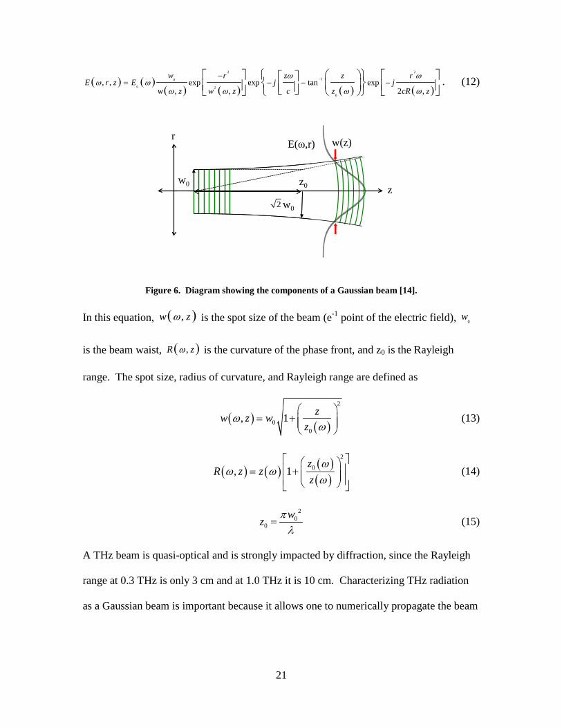
21
( ) ( )( ) ( ) ( ) ( )
2 2
10
0 2
0
, , exp exp tan exp, , 2 ,
w r z z rE r z E j j
w z w z c z cR z
ω ωω ω
ω ω ω ω
−−= − − −
. (12)
Figure 6. Diagram showing the components of a Gaussian beam [14].
In this equation, ( ),w zω is the spot size of the beam (e-1 point of the electric field), 0w
is the beam waist, ( ),R zω is the curvature of the phase front, and z0 is the Rayleigh
range. The spot size, radius of curvature, and Rayleigh range are defined as
( ) ( )
2
00
, 1 zw z wz
ωω
= +
(13)
( ) ( ) ( )( )
2
0, 1z
R z zz
ωω ω
ω
= +
(14)
2
00
wz πλ
= (15)
A THz beam is quasi-optical and is strongly impacted by diffraction, since the Rayleigh
range at 0.3 THz is only 3 cm and at 1.0 THz it is 10 cm. Characterizing THz radiation
as a Gaussian beam is important because it allows one to numerically propagate the beam
z
r
w0 z0
w02
w(z)E(ω,r)

22
through a system of lenses given an initial spot size and radius of curvature at the exit of
the emitter’s hemispherical lens.
2.3.2.4 Gaussian Beam Expansion
A Gaussian beam can be represented in terms of the curvature of its phase front R
and the spot size of the beam w by the complex beam parameter q. The equation for this
relationship is
( ) ( ) ( )2
21 1, , ,
cj
q z R z w zω
ω ω ω= − . (16)
The complex beam parameter can then be used to propagate the Gaussian beam through
an optical system by the use of the ABCD matrix formalism. The output complex beam
parameter outq can represented in terms of the input inq :
1
11
in
out
in
C D qq A B q
+ = +
. (17)
The ABCD matrix has the following format for propagation:
10 1
A B dC D
=
free space (18)
1 01 1
A BC D f
= − lens or mirror (19)
The ABCD matrix formulism allows one to represent an entire optical system by
multiplying a series of propagation matrices together.
d

23
2.3.3 Scanning Optical Delay Line
The THz TDS system requires a means of varying the delay of one optical beam
relative to a second beam in order to move the sampling gate across the waveform to be
sampled. This is accomplished by varying the optical path length traversed by the two
beams by using a scanning optical delay line on one of them. The optical delay is
achieved by mounting a retro-reflective mirror on a mechanical scanner. For this
application, a Newmark NLS4 mechanical stage, remotely controlled by a computer, was
used to scan an 8 cm diameter retro-reflective mirror. The delay line has a maximum
speed of 2 inches/second, a resolution of 0.125 μm, and a repeatability of 5 μm.
In many imaging applications it is desirable to scan the optical delay as rapidly as
possible in order to increase the waveform acquisition rate. However, there are not many
mechanical devices that can scan faster than a few tens of Hertz. Typical point-by-point
images formed by imaging systems have a data acquisition rate of 20 pixels per second,
which translates to a few minutes per image, if one uses a raster scanner to move the
sample through the THz beam [48].
2.3.4 Raster Scanner
A Newmark NLS4-x-25 horizontal and an NLS4-x-16 vertical stage were
connected to form an X-Y stage used to perform a raster scan on various samples for
imaging. The X-Y stage was computer-controlled and could be synchronized with the
scanning optical delay line through the Galil motion control software. The vertical
component had a maximum speed of 0.5 inches/second, a resolution of 0.06 μm, and a

24
repeatability of 5 μm, while the horizontal component had the same specifications as the
scanning optical delay line.
2.3.5 Lock-in Amplifier
A Stanford Research Systems Model SR850 DSP lock-in amplifier was used to
collect electronic data off of the THz detector. The time domain data of the THz pulse
could be measured with either current or voltage. The lock-in amplifier time constant
and optical delay line speed had to be carefully chosen so that the TDS system could
accurately collect the entire pulse, maximize the signal-to-noise ratio, and minimize the
total scan time. The sensitivity and dynamic reserve had to be chosen to maximize the
dynamic range of the lock-in amplifier. Furthermore, the data collection rate and the
optical delay line had to be synchronized to control the bandwidth and frequency
resolution of the THz TDS system. The bandwidth, B, is determined by
( ) 12B t −= ∆ (20)
in which t∆ is the time step between data points collected in the THz pulse. The
frequency resolution f∆ is given by
( ) ( )1 12 2f tN T− −∆ = ∆ = (21)
where N is the total number of points and T is the total time of the scanned pulse.
Finally, “auto-phase” was chosen when collecting the pulse data to adjust the reference
phase shift to eliminate any residual phase error and eliminate the imaginary component.
This maximized the amplitude of the peak of the THz pulse. Data collection could be
25
accomplished by either manual entry of the data through the interface on the front panel
of the lock-in amplifier or through a computer interface using LabView.
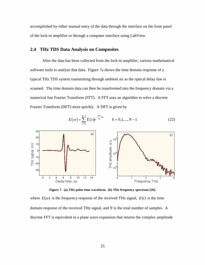
2.4 THz TDS Data Analysis on Composites
After the data has been collected from the lock-in amplifier, various mathematical
software tools to analyze that data. Figure 7a shows the time domain response of a
typical THz TDS system transmitting through ambient air as the optical delay line is
scanned. The time domain data can then be transformed into the frequency domain via a
numerical fast Fourier Transform (FFT). A FFT uses an algorithm to solve a discrete
Fourier Transform (DFT) more quickly. A DFT is given by
( ) ( )21
0 0,1,..., 1
iN tN
tE E t e k N
π ωω
− −
=
= = −∑ (22)
Figure 7. (a) THz pulse time waveform. (b) THz frequency spectrum [26].
where ( )E ω is the frequency response of the received THz signal, ( )E t is the time
domain response of the received THz signal, and N is the total number of samples. A
discrete FFT is equivalent to a plane wave expansion that returns the complex amplitude

26
of the discrete frequency components nω of the THz pulse. This representation of the
THz electric field ( )nE ω can written as
( ) ( ) ( )( )0
n ni k x tn nE E e ω ωω ω − += (23)
where 0E is the amplitude and k is the wave number Figure 7b represents the magnitude
of the Fourier transform of the THz pulse signal in 7a.
In THz TDS, one measures a sample Esamp(t) and a reference pulse Eref(t) in the
time domain and then converts them both into the frequency domain, ( )sampE ω and
( )refE ω , with an FFT. The pulse that is measured at the receiver is a convolution of the
transfer functions of the emitter R(t) and the receiver S(t). The sample also imparts a
transfer function H(t) to the measured THz pulse when it is included in the THz path. A
diagram showing the effect of the sample on the transfer functions in the time and
frequency domains is shown in Figure 8. The convolution of the sample transfer function
in the time domain equates to a multiplication in the frequency domain. An example of
the resulting waveforms in the time and frequency domain is illustrated in Figure 9.
Figure 8. Components of the THz waveform at the detector in the time and frequency domain [14].
( ) ( ) ( ) ( )R S R t S tω ω = ∗ ( ) ( ) ( ) ( ) ( ) ( )R H S R t H S tω ω ω ω= ∗ ∗

27
Figure 9. Waveforms resulting from the collection of data at the THz detector [14].
2.4.1 Material Parameter Estimation
Material parameters, like the index of refraction and the absorption coefficient,
can be measured using a THz waveform. The THz system response of a sample can be
determined by dividing the frequency response of system with a sample ( )sampE ω by the
system response of the reference ( )refE ω . The system response can be shown with the
following equation
( )( )
( ) ( ) ( )( )
( ) ( ) ( )( )( )0
0
0
0
samp
ref
i t k xi k k x
i t k x
E R S ee
E R S e
ω ωω
ω
ω ω ωω ω ω
−− −
−= = (24)
in which 0R is the amplitude of the THz emitter transfer function, k0 is the wave number
in free space, k(ω) is the wave number for the sample material, and x is the length
propagated. The value for k(ω) can be written in terms of its complex parts
( ) ( ) ( )' "k n incωω ω ω= − (25)
and then added to the version of the sample THz system response given in terms of
amplitude A and phase φ
-4
-2
0
2
4
6A
vera
geC
urre
nt(n
A)
0 10 20 30Time (ps)
Eref(t)
Esamp(t)
-4
-2
0
2
4
6A
vera
geC
urre
nt(n
A)
0 10 20 30Time (ps)
-4
-2
0
2
4
6A
vera
geC
urre
nt(n
A)
0 10 20 30Time (ps)
Eref(t)
Esamp(t)
0.00
0.25
0.50
0.75
1.00
Mag
nitu
deof
El e
ctri c
F iel
d
0.0 0.5 1.0 1.5 2.0 2.5Frequency (THz)
|Eref(ω)|
|Esamp(ω)|0.00
0.25
0.50
0.75
1.00
Mag
nitu
deof
El e
ctri c
F iel
d
0.0 0.5 1.0 1.5 2.0 2.5Frequency (THz)
0.00
0.25
0.50
0.75
1.00
Mag
nitu
deof
El e
ctri c
F iel
d
0.0 0.5 1.0 1.5 2.0 2.5Frequency (THz)
|Eref(ω)|
|Esamp(ω)|
( ) ( ) ( )E S Hω ω ω( ) ( )E Sω ω( ) ( )E t S t∗ ( ) ( ) ( )E t S t H t∗ ∗
FFT
28
( )
( )( ) ( )( )' 1"sample
ref
i n xn x iccE
e e AeE
ωω ωω φωω
− −− −= = . (26)
2.4.2 Drude Model
By measuring the THz system response in either transmission or reflection mode,
one can obtain the complex index of refraction of the material. The complex index of
refraction )(~ ωn can be written as
( ) ( ) ( )n n iω ω κ ω= − (27)
where )(ωn represents the real refractive index and )(ωκ is the extinction coefficient
and is proportional to the absorption coefficient )(ωα , which in cgs units is
( )( )2
cα ωκ ωω
= . (28)
One of the ways of predicting the optical properties of a THz TDS system is to use the
Drude Model. The Drude Model offers one method of calibrating a THz TDS system so
that the accurate performance of the system can be verified.
Usually the optical constants of a semiconductor in the far-infrared region are
analyzed with the Drude model. According to the Drude model, the complex
conductivity is expressed as
2
0( ) 1p
i
ωσ ω ε
ωτ
=+
(29)
and in this expression τ is the momentum relaxation time of free carriers and pω is the
plasma angular frequency defined by *0
2 mencp εω = . In this plasma frequency
29
expression cn is the carrier density, e is the charge of an electron, and *m is the effective
mass [67]. The complex electrical conductivity can be written in terms of its real and
imaginary parts: )()()(~21 ωσωσωσ i−= and
1 0 2( ) ( )σ ω ε ωε ω= , (30)
2 0 1( ) [ ( ) ]σ ω ε ω ε ω ε∞= − − (31)
with ∞ε being the relative dielectric constant of the undoped semiconductor and 0ε being
the permittivity of free space [67]. In a nonmagnetic medium, the complex dielectric
constant )(~ ωε is given as
2
0
( )( ) ( )n i σ ωε ω ω εωε
= = −
(32)
and )(~ ωσ is the complex conductivity.
2.4.3 Scattering
Scattering is the process by which electromagnetic radiation is forced to deviate
from a straight trajectory by one or more localized non-uniformities in the medium
through which it passes. There are two types of elastic scattering: Rayleigh scattering
and Mie scattering. Rayleigh scattering is the process by which radiation is scattered by a
small element, treated as a small sphere, in which the diameter d of the sphere is much
smaller than the wavelength λ of the radiation. The upper limit for scattering of this type
is d/λ ~ 1/10. For elements with diameters comparable to the wavelength, Mie scattering
describes the scattering process, and the shape of the scattering elements becomes more
relevant. The study of the propagation and scattering of THz pulses through media has

30
been studied recently [13, 27, 55, 56, 57, 58, 60, 71]. For nondestructive evaluation of
composites with THz radiation, one would be interested in isolating air bubbles, voids,
and delaminations in the material. One could look at the scattering properties of thin
samples and study the multiple-scattering, diffusive, phenomena that can be measured
with coherent pulses. Additionally, the scattering effects of the glass fibers and bundles
within the composite could be studied.
The scattering of coherent THz radiation ( )cohE ω can be described using the
scattering mean free path ( )sl ω as a function of frequency is given by the equation:
( )( ) ( )
( )( )2
4exp exp2 2 1
coh
sin
E zz nlE n
ω α ωωω
− −=
+ (33)
where α is the absorption coefficient and z is the thickness of the sample. The
scattering mean free path is the inverse of the scattering coefficient μs. In order to make
predictions about scattering of THz radiation from particles one would attempt to
determine the scattering cross section ( )sσ ω of the scattering centers:
( ) ( ) 10s sl nω σ ω
−= (34)
in which 0n is the number density of the scatterers in the material.
If the scattering centers are much smaller than the THz wavelength then the
Rayleigh approximation can be used. The scattering cross section for Rayleigh scattering
is independent of the particle shape and is given by
25 6 2
4 2
2 13 2s
d nn
πσλ
−= +
(35)

31
where n is the index of refraction of the scattering centers and d is the diameter of the
spheres. The intensity scattered per unit volume for an unpolarized electromagnetic wave
is given by the following:
( )( )24 6 2
20 2 4 2
1 1 cos8 2s
d nI Ir n
π θλ
−= + +
(36)
where θ is the angle measured from the direction of propagation and r is the distance to
the particle. The scattering efficiency effQ is commonly used in place of the cross section
and is related by
seffQ A
σ= (37)
in which A is cross sectional area of the scattering center. The equation for spheres is
more complicated when the size of the scatterers are closer in size to the wavelength of
the radiation [42].
In composites, there are strands of fiber woven together and then held together
using a resin. The fibers most closely resemble an infinitely long circular cylinder.
When the diameter of the cylinder is sufficiently small compared to the wavelength,
certain approximations can be used for the scattering coefficients. The scattering cross
section per unit length for the TE and TM modes are
( )5 4 223
2 1TMa mπσ
λ= − (38)
25 4 2
3 2
4 11TE
a mm
πσλ
−= +
(39)
where a is the radius of the cylinder and m is the ratio of the index of refraction of the
scattering center to the index of refraction of the containing medium. The samples tested

32
in this research had an overlapping weave pattern of glass strands with all of the strands
oriented in one of two directions at 90° angles to each other. The assumption was made
that the overlapping pattern would result in an average of the scattering cross section of
the TE and TM components, ( ) 2TM TEσ σ σ= + . The intensity of the TE and TM modes
at normal incidence are given by
( )4 4 22
0 3
2 1TMaI I mr
πλ
= − (40)
( )24 4 2
20 3 2
4 1 cos1TE
a mI Ir m
π θλ
−= +
(41)
when the imaginary portion of the refractive index is small compared to the real part.
This illustrates that the intensity of the scattered radiation from infinitely long circular
cylinders varies as the fourth power of the cylindrical radius and inversely as the cube of
the wavelength. This limiting case for infinite cylinders is compared to the intensity of
Rayleigh scattering from small spheres, which varies as the sixth power of the radius and
inversely as the fourth power of the wavelength [42].
The radiation from a photoconductive switch is linearly polarized according to the
orientation of the emitter dipole. For this research, the emitter was oriented for vertical
polarization. If the orientation of the glass fibers is known, then one could predict the
intensity of THz radiation scattering from the glass fiber composite. The TM mode has
its electric field parallel to the axis of the cylinder while the TE mode has its axis
perpendicular to the axis of the cylinder. Using this orientation where the axis of the
cylinder is vertical, one can determine the intensity of THz radiation that is scattered

33
given an incident linear polarization angle. The intensity for the vertically and
horizontally polarized components can be defined as
( ) ( )4 4 22 2
0 3
2 1 sinvaI I mr
π χλ
= − (42)
( ) ( )24 4 2
2 20 3 2
4 1 cos cos1H
a mI Ir m
π θ χλ
−= +
(43)
in which χ is defined as the angle from the positive horizontal axis and r is the radial
distance from the x-axis. A diagram of the configuration is shown in Figure 10 with the
scattered radiation propagating as a cylindrical wave [42]. The glass weave strands could
be oriented at any angle to the THz polarization direction, at normal incidence.
ZIncident
ray
X
Y
θ
Scattered ray
Py
Px
χ
r
Figure 10. Diagram showing incident and scattered ray upon an infinitely long cylinder.
An alternate approach has been presented which models scattering effects within
a densely distributed array of infinite cylinders. Its model utilizes an effective field and a
quasi-crystalline approximation for the multiple scattering interactions within the dense
medium [45].

34
2.4.4 Effective Medium Approximations
The propagation of electromagnetic waves in heterogeneous media can be
analyzed using various effective medium approaches [1, 13, 27, 29, 49, 74]. Among
these approaches, there are variations of three that have been used most frequently,
including the Maxwell-Garnett theory, the Bruggeman effective medium model, and the
simple effective medium approximation. All of these theories assume that spherical
inclusions have been dispersed into a host matrix, the inclusions are much smaller than
the wavelength in the host material (< 0.1λ – 0.2λ), and that the material can therefore be
treated like an effective medium as shown in Figure 11 [6]. The model can also be
extended to cover cylindrical inclusions by using dielectric tensors.
Figure 11. An inhomogeneous system is replaced by a (virtual) effective medium.
The simplest effective medium approach is with linear interpolation, using the
filling factor f, which defines the volume fraction of the particles:
( ) ( ) (1 ) ( )eff i hf fε ω ε ω ε ω= + − (44)
in which iε is the dielectric constant of the inclusions and hε is the dielectric constant of
the host material. Another model that is used is called the Maxwell-Garnett effective
Inhomogeneous Material Effective Medium
εi εh εeff

35
medium theory:
( ) ( )
( ) ( )1 2 / 2
( ) ( )1 / 2
i h i heff h
i h i h
ff
ε ε ε εε ω ε ω
ε ε ε ε
+ − + = − − +
. (45)
This theory assumes that the total polarization should be the same as the sum of
polarization contributions from the embedded particles. The Maxwell-Garnett
approximation holds up well at low filling factors f until the filling factor reaches a level
of approximately 0.15. At this point, the theory developed by Bruggeman must be used
to achieve an accurate determination of the effective dielectric constant. The formula is
given by
(1 ) 0i eff h eff
i eff h eff
f fK K
ε ε ε εε ε ε ε
− −+ − = + +
(46)
where K is a geometric factor. The value for K is 1 if the inclusions are an array of
cylinders with their axes collinear with the incident radiation and the value for K is 2 if
they are spherical nanoparticles [8].
2.4.5 Imaging
The THz wave distribution function and the target’s refractive index can be
described by Maxwell’s Equation:
( ) ( )2 2
22 2
( , ), , , , 0n rE r t E r tc t
ωω ω∂∇ + =
∂
(47)
where r denotes a point in space, c is the speed of light, and n is the complex refractive
index of the medium. In the case where the polarization effects of the wave can be
neglected in the temporal frequency domain, this equation can be written as the scalar

36
Helmholtz equation
2 2 20( , ) ( , ) ( , ) 0E r k n r E rω ω ω∇ + =
(48)
in which E(ω,r) is the complex amplitude function of the electromagnetic field and k0
represents the wave number. This Helmholtz equation is valid in imaging and
tomography applications. The purpose of THz imaging is to determine the refractive
index function ( , )n rω using the measured THz wave amplitude and phase distribution
function E(ω,r) [75].
THz imaging can be performed in either transmission or reflection mode. A THz
TDS imaging system is constructed with a focus at the desired location of the object to be
imaged. The waveform of the THz pulse that goes through the object at that focus can
then be measured. By translating the object and measuring the transmitted waveform for
each position of the object, an image can be built pixel by pixel. The two dimensional
image that is formed may be represented by such aspects of the waveform as amplitude,
phase, or a combination of the two. Phase, or time delay, imaging consists of the
extraction of the arrival time of the waveform at each pixel. For amplitude imaging, one
could use the peak-to-peak amplitude of the time-domain waveform for a measure of
bandwidth-averaged transmission. Alternatively, one could perform an FFT of each
pixel’s waveform and then integrate over any desired frequency band to display some
part of the spectral information [12, 48].
Three-dimensional, THz tomography refers to the cross-sectional imaging of an
object by measuring either the transmitted or reflected illumination. One way of
accomplishing this is to measure the time-domain THz pulse transmitted through or

37
reflected by the material. The resulting waveform will consist of a series of reflections
from the sample of the various dielectric interfaces within that sample. The polarity and
magnitude of each reflection are given by the reflection coefficient at each interface and
are related to the size and sign of the corresponding index step [48]. This form of THz
tomography is restricted, though, in its applicability. This type of tomography is based
on three assumptions: (1) the samples have no dispersion, absorption, or diffraction
affects, (2) the reflections are so weak that multi-reflections can be neglected, and (3) the
refractive index is uniform throughout each layer [75]. Any one of the affects listed can
significantly alter the shape of the reflected waveform. A numerical Fourier
deconvolution in the time-domain could be applied to the waveform to more accurately
measure the position of each of the reflections. Other methods of tomography are
diffraction tomography, computed tomography, binary lens tomography, optical
coherence tomography, and digital holography [75].
2.4.6 Image Processing
The image of a composite sample can be formed by arranging the pixels that were
collected during the THz TDS scan. Since THz images are formed from a limited
number of samples, their images appear “pixelated.” Interpolation techniques can be
employed which enable one to remove the sharp edges of the pixels to make the image
easier to view visually. Interpolation is the estimate of a signal at locations other than
where it was sampled. If a two dimensional array’s pixels are expanded equivalently in
both dimensions, the interpolation is called zoom or electronic zoom. Various

38
interpolation techniques in the time domain include the ideal sinc, zero order, triangular,
or cubic spline interpolator [32].
A frequency domain interpolation technique was applied for the THz images in
this research. The sampling rate was increased by zero-padding in the spatial frequency
domain. First, the two-dimensional image can be transformed to the frequency domain
with a discrete cosine transform (DCT). A DCT is similar to the discrete Fourier
Transform (DFT) except that it uses only the real numbers, and is frequently used in data
compression algorithms because it tends to concentrate information. Then the resulting
matrix can be zero-padded in the spatial frequency domain which increases the sampling
rate in the spatial domain. Finally, an inverse DCT can be performed on the data which
results in the display of much smaller pixels and an apparent smoothing of the original
pixel edges. By using the interpolation technique outlined above, zero-padding out to ten
times the length and width in the frequency domain, the new image will appear to look
the same as if the original image was shrunk ten times.
MATLAB also has a function called ‘interp’ which is designed to smooth
boundaries between pixels. However, when this function is used on its own, it tends to
create a blurry image if the pixels are too large. Occasionally, the DCT can leave a
periodic pattern in the image from sharp boundaries which can be further smoothed out
with a filter. A filter that has been used successfully for THz imaging by Zhang et al. is
the Wiener filter [75].

39
2.5 THz TDS Literature Review
This section summarizes some of the recent work that has been published on the
NDE of materials using THz TDS and on the progress in modeling the THz electrical and
optical properties of those materials. This is followed by a summary of some of the work
done on imaging and on characterizing the THz properties of composites, ceramics, and
semiconductors, as well as paint and foam adhering to metallic surfaces.
2.5.1 Composites
A composite is defined in the American Heritage Dictionary as: “A complex
material, such as wood or fiberglass, in which two or more distinct, complementary
substances, especially metals, ceramics, glasses, and polymers, combine to produce
structural or functional properties not present in any individual component” [3].
Composite designers can choose from a variety of fiber reinforcements and resins to
develop the laminate structure. The reinforcement material provides mechanical
properties such as stiffness, tension and impact strength, while the resin system (matrix)
provides physical properties including resistance to fire, weather, ultraviolet light and
corrosive chemicals. Three factors must be considered when choosing reinforcements.
One must first choose the type of fiber: usually fiberglass, aramid (in Kevlar), or carbon
fiber (also called graphite). Then one must choose the form: either roving strands, mat,
or fabrics. Finally, an orientation of fiber direction is chosen, including parallel,
circumferential, or helical along the length of the part, and/or with random continuous
strands. The three types of resins that are available are polyester, vinyl ester, and epoxy.

40
A form, either wet lay-up or prepreg (a reinforcement saturated with resin), must be
carefully chosen to ensure a successful design [78].
Several articles have been written describing the response of THz radiation when
transmitted through various composites. One of the types of composites that has been
studied involves polymers, which can be mixed with other additives or fillers to yield
compounds with modified physical properties. In the manufacture of these composites, it
can be difficult to verify the degree of homogeneity of the resulting compound, especially
when using nanoscale fillers. One research group studied samples of low-density
polyethylene (LDPE) containing titanium dioxide nanospheres (diameter ~ 270 nm)
coated with silver nanoparticles (~ 20 nm) as well as glass-fiber reinforced with epoxy
[64, 66]. For the first case, they were able to see inhomogeneous areas in the LDPE
polymer, but were not able to unambiguously determine whether the inhomogeneities
were a result of the internal content or the surface reflections from the rough surface. In
the case of the glass fiber matrix, THz TDS was able to locate materials and defects
hidden inside the sample. A separate article characterizes the refractive index and
absorption coefficient of polymers, including high-density polyethylene, Picarin, and
cyclic olefin polymer [69]. All of these polymers can be used to fabricate THz
communication systems. The authors showed that up to 90% of the incident THz
radiation passes through 2 mm of each of the materials with very little attenuation,
making them good candidates.
Another composite that has been studied is the polymer-graphite composite [70].
These types of composites are excellent absorbers of THz radiation with good shielding
efficiency and small reflection. THz TDS was used to measure the complex refractive

41
index of this composite, showing that with a 35.7% graphite concentration, reflection was
less than 10%, while the absorption was over 80%. Finally, a separate study has been
conducted on aerospace carbon-fiber composites and space shuttle insulating tiles,
exploring the effectiveness of using THz radiation for NDE of heat damage and voids
[62]. The article was focused primarily on comparing continuous wave (CW) THz
techniques to pulsed techniques, showing that CW THz systems have sufficient
resolution to detect voids and heat damage.
2.5.2 Ceramics
Although ceramics can be considered a subset of composites, a ceramic is more
specifically defined in Wikipedia as “an inorganic non-metallic material whose formation
is due to the act of heat” [78]. Ceramics are used in a wide range of applications
including jet engines and mirrors. Silicon carbide (SiC) is a ceramic material which is
strong and light-weight and is an excellent choice to be used for space-based mirrors. It
is a difficult material to mount, and the unrelieved stress that results from mounting can
cause failure during launch. The photoelastic effect, measured in the THz spectrum, can
be used to measure the stress induced in the SiC. Recent literature has shown that the
photoelastic effect has been used effectively to characterize defects in silicon carbide
wafers in the optical regime [43, 46].
Studies have recently been conducted using THz TDS on aluminum oxide
bearings and glass ceramics to measure their optical constants and to probe them for
existing fractures [62, 63, 68]. Measurements have also been made on the dielectric
constants and loss tangents of low-loss, high dielectric constant ceramics at THz

42
frequencies [11]. The materials tested included alumina, steatite, titania loaded
polystyrene, and zirconium-tin-titanate. The real part of the dielectric constants of these
materials were 6.5, 9.3, 16, and 37-93 respectively for each of them and could be used for
cost effective photonic crystal components. Finally, material parameters were measured
on various building materials, like plaster, glass, and wood [59].
2.5.3 Paint Thickness over Metallic Surfaces
The external coating of nearly all military aircraft is stripped down to bare metal
during programmed depot maintenance cycles. This paint stripping process has become
cost prohibitive in recent years and continues to be a major problem for the sustainment
of aging aircraft fleets. One of the main contributing factors is the requirement to
visually inspect aircraft for corrosion and fatigue damage. Several nondestructive
techniques have been used to avoid visual inspection, including infrared, eddy current,
ultrasonic, radiographic, and near-field microwave. THz offers the advantage of being
non-contact, penetrating nonconductive materials, and reflecting from both metallic
materials and from impedance discontinuities like voids and inclusions [16].
One paper presented an approach to use THz tomography to measure the
thickness and degree of drying in the painting process. The thickness resolution mind is
the limiting factor when using THz radiation and is given by
min ( ) /(2 )gd c T n= ∆ (49)
where c is the speed of light in a vacuum, T∆ is the temporal width of the THz pulse,
and gn is the group index of refraction for the medium [87]. This paper reported that the
resolution was limited to ~ 10 μm. Another paper reported that surface roughness

43
differences below ~ 10 μm were indistinguishable from the metallic background when
searching for corrosion under paint [5].
2.5.4 Semiconductors
THz TDS can also be used to measure the optical and electrical properties of a
semiconductor by the technique outlined in section 2.4.1. Such techniques have been
applied to various semiconductor materials and their nanostructures, including quantum
dots [54], photonic crystals, and carbon nanotubes, which can have both metallic and
semiconductor properties. Photonic crystals, made from semiconductor materials, have
been studied recently using THz TDS to determine both defects and group velocity and
group velocity dispersion characteristics [37, 38, 39, 53]. The dielectric constant of
carbon nanotubes has been measured with a combination of the Drude and Lorentz
harmonic oscillator models [41, 47]. In the dielectric function ( )ε ω shown in the
following equation, the second term in the sum represents the Drude model and the third
term represents the Lorentz model:
2 2
,2 2 2( )
( )p p L
L Li iω ω
ε ω εω ω ω ω ω∞= − +
+ Γ − − Γ. (50)
The term ε∞ is the dielectric constant at infinity, ωp is the plasma frequency, Γ is the
damping rate in the Drude model, ωL is the phonon frequency, LΓ is the spectral width,
and ωp,L is the strength of the Lorentz oscillator. Further characterization using the Drude
model could also allow one to determine the number of photocarriers which have been
generated.

44
Carrier dynamics can also be determined by using a technique called Optical-
pump THz-probe spectroscopy to measure the conductivity of photocarriers as a function
of time after photoexcitation [2, 10]. In this photoluminescence setup, an additional
probe beam from the laser source is used to optically illuminate the sample and generate
carriers so that it can then be probed with a THz beam. The optical-pump THz-probe
technique has been used extensively to study semiconductor carrier dynamics. It has also
been used to measure the optical and electronic characteristics of the material by using
the free electron Drude model or the Lorenz model to estimate the dielectric constant.
2.5.5 Measuring Material Properties with THz Radiation
Significant efforts have been expended on the development of THz imaging
systems; however, somewhat less attention has been paid to the issue of the propagation
through, or scattering from, realistic target materials which might be investigated with
such systems. Understanding the interaction of THz radiation with a wide range of both
homogeneous and inhomogeneous materials is an essential part of the design of systems
for THz sensing and imaging. This section attempts to provide a summary of some of the
recent work done on modeling the scattering of THz radiation and on the estimation of
material parameters using THz TDS.
2.5.5.1 Transmission Mode Measurement Technique
One method of determining the material parameters of a homogeneous, planar
material in using THz TDS in transmission mode is outlined by Dorney et al [23]. A
schematic of the interaction of a THz pulse with a sample is shown in Figure 12. An

45
incident pulse contacts the sample where part of the wave is reflected and part is
transmitted. As the THz wave propagates through the material it interacts with that
material. Multiple reflections can also occur at the internal interfaces of the material,
creating multiple output pulses.
Figure 12. Transmission and reflection of a THz wave through a planar, homogeneous material.
The Fresnel equations describe the transmission and reflection of the THz wave at
each interface
2 ( ) cos( )( ) cos ( ) cos
aab
a b
ntn n
ω θωω β ω θ
=+
(51)
( ) cos ( ) cos( )( ) cos ( ) cos
b aab
a b
n nrn n
ω θ ω βωω β ω θ
−=
+
(52)
where ( )abt ω is the transmission coefficient of a wave at an incident angle θ from region
a to region b and ( )abr ω is the reflection in region a at the a-b interface. The angle θ is
estimated and the angle β is an approximation of Snell’s law for nearly transparent
materials:
m
l
d
Air AirSample
θ
θβEinitial
r01
Eprimary
E1st multiple
E2nd multiple
t01 t10
psample

46
sinarcsin a
b
nn
θβ
=
. (53)
As the wave moves through the material along the path designated d, it accumulates a
phase change through given by ( , )dp dω according to a transfer function or THz system
response
( )( , ) exp bd
in dp dcω ωω − =
(54)
where c is the speed of light and the ray length d is determined by
cos
ldβ
= . (55)
Scattering is neglected in this model including such effects as the interface roughness
[23].
The THz path both with and without the sample must be considered. For the free-
air path, or reference path, we have
( ) ( ) ( , )ref initial airE E p xω ω ω= (56)
with the distance x being the distance between the transmitter and receiver and nair being
the index of refraction of air (1.00027). For the propagation through a sample, the
distance m through the sample must be subtracted from the distance traveled through air.
This distance varies with the angle of incidence and the material parameters. This
distance m is defined as:
cos( )m d θ β= − . (57)
In Figure 12 there are only two additional paths shown representing the Fabry-Perot
effect, but several additional paths could also be shown. The equation for the primary

47
received signal through the sample is given by
01 10( ) ( ) [ , ( )] ( , )primary initial air sampleE E p x m t p d tω ω ω ω= − × . (58)
In this expression, 01t is the transmission coefficient at the air-sample interface and 10t is
the transmission coefficient at the sample-air interface. Now that we have both the
reference wave and the sample wave defined, we can define the ratio of the two
2
( ) 4 ( ) ( ) co s co s [ ( ) ( )]exp
( ) [ ( ) co s ( ) co s]primary air sample sample air
ref air sample
E n n i dn mn
E n n c
ω ω ω θ β ω ω ω
ω ω β ω θ
− −= ×
+
. (59)
This provides the transfer function for the model, where only the complex function for
( )samplen ω , l, and θ are free variables [23].
This procedure, outlined by Dorney et al., involves a three step iterative process
of determining the thickness and the complex index of refraction. The first step is to
make an initial guess at the thickness of the sample. Second, the algorithm calculates the
beginning functions for the complex index of refraction, assuming a non-dispersive
medium. Finally, a gradient descent algorithm iterates the complex index of refraction in
frequency until the total error no longer decreases monotonically. The complex index of
refraction is then computed in this manner for a range of thicknesses. A metric called
total variation is then used to select which pair of refractive index and thickness should
be selected [23].
2.5.5.2 Literature Summary of THz Material Parameter Measurements
The technique for modeling the material parameters of a homogeneous, planar,
optically thin, low-absorption material is shown in section 2.5.5.1. This technique was
designed by Duvillaret et al. and refined by Dorney and Mittleman [22 - 25]. Although

48
Duvillaret et al. claim that an accurate initial guess at the sample thickness is very
important to determine the material parameters, Dorney et al. claim that they are able to
accurately determine sample thickness and refractive index by initially bounding the
upper and lower limits of the thickness l
1 2
,upper lowerair air
tc tcl ln n n n
∆ ∆= =
− − (60)
in which t∆ is the time delay between the reference pulse and the first pulse from the
sample. The parameters 1n and 2n are the limits of the range of refractive index, of
which the range 1.2 – 8 covered most practical cases [23]. Withamayachumnankul et al.
were able to use a fixed-point iterative method to determine the complex refractive index
of the sample within a few iterations, given the sample thickness. Using the same
measurement techniques as Dorney and Duvillaret, their iterative process gave the correct
parameters for a silicon wafer sample when the material thickness exceeded 200 μm [79,
80].
Xu et al. prepared a simulation with a Lorentz oscillator model to evaluate the
accuracy of the extracted optical constants in THz TDS [85]. They analyzed the
influence of the angle deflection, the delay-line timing error, and background and 1/f
noise on the THz TDS measurement precision. They found that the deflection of the
incident angle can influence both the real and imaginary parts of the index of refraction
and the spectral features of the errors show a parabolic shape. They also found that the
delay-line timing uncertainty introduced an exponential-dependent deviation curve of the
imaginary part in the frequency domain and a dramatic feature in the resonant region for
the real part.

49
A separate study reported on the propagation of a single-cycle THz pulse in a
random media. Pearce et al. demonstrated a unique method for characterizing the
diffusive radiation emerging from a random medium, involving the measurement of both
its amplitude and phase [56]. They were able to compute a time-windowed temporal
correlation between fields measured at different spatial locations which enabled them to
identify individual scattering events for imaging applications. Pupeza et al. have
developed a refined approach to measuring optical material parameters [61] while Kuzel
et. al. has extracted both the complex refractive index and the wave impedance using THz
TDS [44].
2.5.6 THz TDS for NDE
This subsection outlines some of the recent literature reported specifically on the
use of THz for NDE and quality control. In composite research, fiber glass samples from
the automotive industry have been analyzed for their material property characteristics and
have been imaged to show damage from stress [64, 66]. Some of the polymers that are
typically used as the matrix material in composites have also been researched [76, 77].
The first article looks at the use of THz imaging to inspect plastic weld joints. They were
able to use THz TDS to reveal contaminates like metal or sand within a weld joint of two
polyethylene sheets and to identify small air gaps where the welding process had failed.
In the second article, the authors were able to determine the additive content of polymers
used in composites, including magnesium hydroxide in polyethylene, glass fibers in
polyamide, and calcium carbonate, silicon or silicon dioxide in polypropylene.

50
THz NDE is also being proposed as a method of inspecting the adhesive bond-
line of space shuttle tiles for defects [4, 84, 92]. Space shuttle tiles are manufactured
from silica into a very porous material. These tiles are then bonded to the bottom of the
space shuttle to provide insulation for re-entry. A triangular shaped defect was identified
using data from a THz NDE scan and post-processing with a Hilbert-Huang Transform
[4]. This process successfully highlighted the boundary between the triangular shaped
defect and the background.
There are other articles which have been written to describe the use of THz TDS
for NDE of materials other than composites. One of the authors presents work using THz
TDS in reflection mode to inspect mural paintings for damage. They are able to image a
sub-surface painting of a butterfly hidden beneath various colors of paint [34]. A
separate application uses THz TDS to detect foreign bodies in chocolate bars, including
metallic objects, stone, glass, and plastics. It can also distinguish these objects from nuts
and other food products within the bars [40].

51
3. Material Parameter Estimation with Terahertz TDS
In the nondestructive testing of aircraft composites, one is ultimately interested in
identifying damage, including damage from heat and mechanical stress, and the detection
of voids and delaminations. Measuring the material properties of a composite provided
insight into the fundamental interaction of THz radiation with the material and could be
tested as a technique to see if the material properties of a damaged composite were
changed. A major focus of this chapter is to present the results obtained when THz TDS,
in transmission and reflection configuration, was used to measure the index of refraction
and absorption coefficient of various materials. In addition, scattering and effective
medium theory were studied for their applicability to composites. Finally, this material
parameter measurement technique was applied to composite samples with burn damage.
3.1 THz TDS System Characterization
There were several challenges associated with setting up a THz TDS system,
including the accurate alignment and measurement of laser pump and probe beams, THz
beam alignment, and the maximization of THz output signal quality. A diagram of our
first setup for material parameter measurements is shown in Figure 13, using only two
parabolic mirrors since the beam did not need to be focused onto the samples. To
determine the point at which the TDS system measurements were of sufficient quality,
we started with an initial set of criteria for comparison. The next sections will detail
these criteria and the methodology for analyzing the THz output, including the
measurement of water absorption spectra. This will be followed by a subsection on the

52
modeling of the THz pulse and associated spectrum. This will be followed by an
explanation of some of the difficulties that we had initially with the PCA detector and of
the techniques that we used to help align the THz TDS system more quickly.
Figure 13. THz TDS setup for material parameter measurements.
3.1.1 THz TDS Output Specifications
The output specifications that we used to help evaluate our THz TDS system were
detailed by Cheville et. al. in their THz tutorial [14]. These criteria are compared in
Table 1 along with the measured results from our THz TDS setup. Although one could
measure the signal-to-noise ratio from a logarithmic plot of the THz amplitude spectrum,
Cheville et. al. recommend measuring the signal-to-noise ratio and the dynamic range in
the time domain. The signal-to-noise level was measured by fixing the optical delay line
Femtosecond Laser(Mode-locked Ti: Sapphire)
Sample
Nd:YVO4 Freq. DoubledPump Laser
Diode Pump Laser
Scanning
Optical
Delay Line
THz Transmitter
ZnTe Crystal
Lock-inAmplifier
Probe (Grating) PulsePump
Pulse
THz Emission
Pellicle Beam splitter
f = 6 cm
100 femtosecondpulse
λ/4 Plate
Power Supply
50 V, 100 kHz
Wollaston PrismWollaston Prism
Balanced Photodiodes

53
at the position of peak pulse amplitude and then collecting data for 30 minutes at that
position. One could then measure the mean of the peak amplitude and observe how much
the signal drifted. The signal-to-noise ratio is given by
2
pk mean
pk
VSignalVNoise−=
∆
(61)
when the THz signal is measured in volts. The dynamic range is then measured by
collecting a scan of the pulse, making sure to take sufficient time domain data in front of
the pulse (t < 0). The data is then scanned to find the smallest voltage step in this period
prior to the pulse and is then compared to the peak of the pulse
min( 0)
pk
t
Vdynamic range
V <
=∆
. (62)
The measurement accuracy specification was made by comparing 10 separate THz TDS
scans and comparing the absolute variations in the amplitude spectra between them.
Table 1. THz Time Domain Spectrometer specifications and measurements. Specification Typical Value Conditions AFIT Typical
Measured Value Amplitude
Dynamic Range 20,000:1 Measured in time domain 14,000:1
Power Dynamic Range
400,000,000:1 Amplitude value squared 196,000,000:1
Median Frequency
0.654 THz Determined by spectral amplitude
0.704 THz
Bandwidth
0.06 to 2.51 THz 0.12 to 1.64 THz 0.26 to 0.92 THz
2% points of peak amplitude 10% points of peak amplitude 50% points of peak amplitude
0.01 to 2.5 THz 0.05 to 1.9 THz
0.15 to 1.35 THz Signal-to-Noise (Signal Drift)
± 0.5% from mean Measured sitting at peak of pulse over 30 minute period
± 2.75% from mean standard deviation
= 0.9%
Measurement Accuracy
± 0.5% @ 0.2 THz ± 0.5% @ 0.5 THz ± 0.25% @ 1 THz
± 2% @ 2 THz
No signal averaging, 10 minute scan length
±3.23% @ 0.2 THz ±0.22% @ 0.5 THz ± 5.14% @ 1 THz ± 20% @ 2 THz

54
3.1.2 Water Vapor Absorption Spectra
Another method that was used to determine if our THz TDS setup was producing
accurate results was to look at water vapor absorption spectra. The water vapor in the
atmosphere leaves fluctuations after the main pulse in the time domain and it leaves
characteristic notches in the frequency spectrum. A full scan of the THz pulse through
air was taken by moving the optical delay line at a slow rate. The results of the scan are
shown in Figure 14. It should be noted that the smaller pulse in 14a is a result of
reflections in the ZnTe crystal which cause the Fabry-Perot etalon effect in 14c. The
phase plot in 14b shows how the phase unwraps linearly with frequency.
(a) (b)
(c)
Figure 14. THz TDS scan of ambient air: (a) THz time domain pulse, (b) THz phase spectrum, and (c) THz amplitude spectrum.

55
The absorption lines in 14b can now be identified in the THz frequency spectrum and can
be compared with those measured and calculated in the literature. As shown in Table 2,
our absorption lines line up fairly closely with published values between 1.0 – 2.4 THz.
Several articles have been written measuring the absorption spectrum of water at various
relative humidity readings and studying the various molecular transitions and phenomena
associated with absorption [83, 90].
Table 2. Absorption spectrum rotational transitions for water vapor between 0.2 – 2.4 THz [82]. Transition Number
Published Frequency
(THz)
Measured Frequency
(THz)
∆ν (THz) Published - Measured
1 0.557 0.56 -0.003 2 0.753 0.75 0.003 3 0.989 0.99 -0.001 4 1.098 1.10 -0.002 5 1.164 1.16 0.004 6 1.2264 1.23 -0.0036 7 1.4116 1.41 0.0016 8 1.603 1.60 0.003 9 1.671 1.67 0.001 10 1.718 1.71 0.008 11 1.798 1.80 -0.002 12 1.869 1.87 -0.001 13 1.921 1.92 0.001 14 2.076 2.07 0.006 15 2.264 2.27 -0.006 16 2.346 2.35 -0.004 17 2.393 2.40 -0.007
3.1.3 THz Pulse and Spectrum Modeling
The shape of the THz pulse was very sensitive to the position and alignment of
the laser pump and probe beams as well as the THz optics. One could attempt to predict
the shape of the THz beam in both space and time by approximating it as a Gaussian

56
pulse. In one article, the authors have already attempted to model the effects of EO
sampling on a Gaussian pulse emitted from a GaAs crystal and detected by a ZnTe
crystal [9]. Beside the effect of the THz emitter and detector, both the alignment of the
lenses and mirrors as well as the sample have an effect on the eventual shape of the pulse.
In this exercise, the emphasis was on modeling the effects of a glass fiber composite
sample on the THz pulse and comparing modeled data to measured data.
When pulses reach the single cycle regime, like they do with THz TDS, one must
use the following equation to model the electric field E(r,t) of the pulse:
( ) ( ) ( )2 21 00 1 0
2, exp exp exp2 2
GG
G G
t i tw rE r t
Lvη ω τ ηω τ
τ τ
− − =
(63)
where 0w is the spot size of the THz beam, 1ω is the central frequency of the THz
spectrum, 0Gτ is the pulse duration, r is the distance from the center of the beam, L is the
distance the pulse has traveled, and v is the speed of the pulse through the medium
modified by the complex index of refraction [19]. The terms ( )tη and Gτ are defined as:
( )2
2L rt tv Lv
η = − − and (64)
22 0
0G Gw rLc
τ τ = +
. (65)
In modeling the THz pulse shape in the time domain, the spot size was assumed to
have a width 0w of 0.6 mm which became mostly irrelevant when considering the center
of the THz spot at r = 0. Both the THz pulsewidth and frequency center of mass had to
be measured from actual data. Data was chosen carefully so that the majority of the pulse

57
had a positive polarity like a Gaussian. The full width at half maximum (FWHM) value
of 0Gτ was measured to be 0.62 psec and the THz central frequency was 0.55 THz.
After choosing the THz signal characteristics, the Gaussian pulse through the air
reference was modeled in the time domain and frequency domain. The glass fiber
complex index of refraction was applied to the frequency domain data using ( )2.05 iK ω−
where K(ω) is the imaginary part of the index of refraction. Then an inverse Fourier
transform was applied to return the pulse to the time domain. The comparisons of the
modeled and measured pulses and frequency spectra can be seen in Figure 15. Although
a Gaussian distribution for the pulse was assumed, the FWHM value 1.177G pτ τ= for a
Gaussian was not small enough to match the measured frequency response. A factor of
1.763G pτ τ= , similar to a sech distribution, was more accurate in modeling the THz
pulse and spectrum characteristics. The magnitude of the modeled air reference pulse
was chosen to match the peak-to-peak amplitude of the measured THz pulse. It is
apparent that factors other than the sample have an effect on the THz signal, such as the
THz emitter, detector, optics, and water vapor absorption.
Figure 15. Comparison of a Gaussian modeled THz pulse through air and glass fiber compared to THz TDS measurements for air and glass fiber in the (a) time domain and (b) frequency domain.

58
3.1.4 System Setup Challenges
The most challenging part of collecting data from a THz TDS system is the
alignment of the optical components with the near-infrared laser and the terahertz beam.
The laser has to be aligned with the photoconductive switch antenna and with the detector
(either a photoconductive switch or an electro-optic crystal). Then the THz beam had to
be aligned through the optical system of parabolic mirrors to maximize the THz pulse
received at the detector. One piece of equipment that was essential to the THz beam
alignment was a pyroelectric detector. This pyroelectric detector could be used to
maximize the beam intensity at each of the optical components before locking them into
place and helped to manage the many degrees of freedom that existed in the alignment
problem. A HeNe laser could be used to initially help align the near-infrared Ti:Sapphire
laser with the emitter and detector. Then fine-tuning of the position of the laser spot
could be steered by measuring the resistance of the emitter and detector. The laser power
sent to the pump and probe beams also had to be closely monitored so that the maximum
specifications were not exceeded. A list of the specifications that were measured are
listed in Table 3.
Table 3. List of Specifications for Ekspla photoconductive switch components. Measurement Measured Value Maximum Limit/
Expected Value Emitter Dark Resistance Infinite Infinite
Emitter Illuminated Resistance 3.1 MΩ 8 MΩ Detector Dark Resistance 68 MΩ 67 MΩ
Detector Illuminated Resistance 1.3 MΩ 0.8 MΩ Pump Laser Power 125 mW 125 mW Probe Laser Power 50 mW 50 mW
Power Supply Voltage 50 Volts 50 Volts Power Supply Modulation 120 kHz 50 kHz

59
Significant effort was expended to align the Ekspla photoconductive detector,
before it was considered damaged or unusable. The pulse widths that were measured
were much wider in the time domain and much lower in amplitude than the advertised
values in the Ekspla manual. Figure 16 shows the (a) THz pulse and its (b) amplitude
spectrum measured at the photoconductive switch receiver. In the time domain, the main
pulse was spread out over 6 psec and several oscillations proceeded for a long duration
after the main pulse.
(a) (b)
Figure 16. THz pulse measured with photoconductive (PC) switch detector: (a) time domain pulse and (b) frequency domain spectrum compared to electro-optic detector.
It was also two orders of magnitude lower in amplitude than the pulse measured with the
ZnTe crystal. This translated to a narrower bandwidth (~0.7 THz) and a reduced
amplitude in the frequency domain. The energy in the pulse was determined by
estimating the noise floor for each spectrum and then calculating the area under the curve
above the noise floor for each spectrum separately. The total energy under the PC switch
spectrum was only 2% of that under the EO detector spectrum.
3.2 Transmission Mode Measurements
This section outlines the results of our transmission mode measurements of
optical parameters using THz TDS. The first two subsections show the calculation

60
techniques used to determine the material parameters and the results of those
calculations. The last subsection shows how to use the Drude model to calibrate the
material parameter measurements from the THz TDS system using a semiconductor.
3.2.1 Calculation Technique
Although the theory for calculating materials parameters was discussed in section
2.4.1, the practical technique used in this research for determining indices of refraction
and absorption coefficients is outlined in this section. The index of refraction ( )n ω was
calculated using the following equation
( )( ) ( )
1 sam ref
sam
cn
dφ ω φ ω
ωω
− = + (66)
where φ is the phase of the sample (sam) or the reference (ref), c is the speed of light,
and samd is the sample thickness. One of the challenges of using this formula was to
accurately unwrap the phase data linearly between the sample and reference since
software routines alternate between –π and +π. The absorption coefficient ( )α ω could
be calculated using the following formula
( ) ( )( ) ( )
2 ln sam
sam ref
Ed T E
ωα ω
ω ω
= −
(67)
in which ( )samE ω is the magnitude of the THz field collected through the sample, and
( )refE ω is the magnitude of the THz field collected through air. ( )T ω is the fraction of
the power transmitted through the air-sample interface given by

61
( ) ( )( )( )2
4
1
nT
n
ωω
ω=
+. (68)
The index of refraction and the absorption coefficient could be determined with an
iterative process, solving both of them simultaneously at each frequency component.
Since the absorption coefficient calculations were somewhat noisy, a windowing filter
could be applied which averaged the ten nearest data points at each frequency.
When making material parameter measurements, one must also pay attention to
the dynamic range DR of the THz TDS setup. The largest absorption coefficient that can
be measured reliably with a given DR corresponds to the situation in which the sample
signal is attenuated to a level equal to the noise floor:
( )max 2
42ln1nd DR
nα
=
+ . (69)
If the absorption coefficient exceeds maxα then the analysis will show an apparent
absorption coefficient equal to maxα . The index of refraction is not subjected to the same
limitations [35].
Experimental uncertainty or error is another consideration in making calculations
with measured data. One must first estimate the measurement error for all of the
potential sources, given as δx, δy, etc. If the source of uncertainty is from a standard
deviation, it can be adjusted by the factor 1/ n if n is the total number of runs. Once
this is accomplished then the total error δf of a function f can be expressed by
22
2 2 ...f ff x yx y
δ δ δ ∂ ∂ = + + ∂ ∂
. (70)
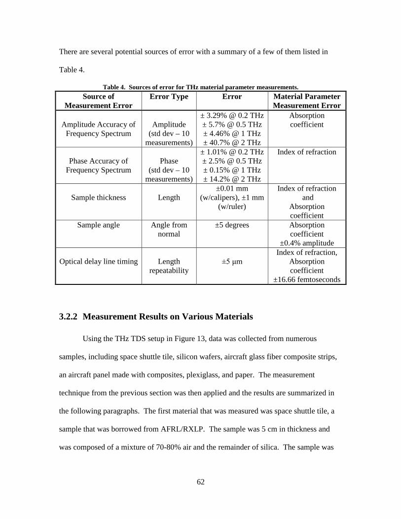
62
There are several potential sources of error with a summary of a few of them listed in
Table 4.
Table 4. Sources of error for THz material parameter measurements. Source of
Measurement Error Error Type Error Material Parameter
Measurement Error
Amplitude Accuracy of Frequency Spectrum
Amplitude
(std dev – 10 measurements)
± 3.29% @ 0.2 THz ± 5.7% @ 0.5 THz ± 4.46% @ 1 THz ± 40.7% @ 2 THz
Absorption coefficient
Phase Accuracy of
Frequency Spectrum
Phase
(std dev – 10 measurements)
± 1.01% @ 0.2 THz ± 2.5% @ 0.5 THz ± 0.15% @ 1 THz ± 14.2% @ 2 THz
Index of refraction
Sample thickness
Length
±0.01 mm (w/calipers), ±1 mm
(w/ruler)
Index of refraction and
Absorption coefficient
Sample angle Angle from normal
±5 degrees Absorption coefficient
±0.4% amplitude
Optical delay line timing
Length repeatability
±5 μm
Index of refraction, Absorption coefficient
±16.66 femtoseconds
3.2.2 Measurement Results on Various Materials
Using the THz TDS setup in Figure 13, data was collected from numerous
samples, including space shuttle tile, silicon wafers, aircraft glass fiber composite strips,
an aircraft panel made with composites, plexiglass, and paper. The measurement
technique from the previous section was then applied and the results are summarized in
the following paragraphs. The first material that was measured was space shuttle tile, a
sample that was borrowed from AFRL/RXLP. The sample was 5 cm in thickness and
was composed of a mixture of 70-80% air and the remainder of silica. The sample was

63
scanned and the resulting pulses and amplitude spectra are shown in Figure 17. One can
observe that the amplitude of the pulse is reduced and the pulse broadens after traveling
(a) (b)
Figure 17. THz TDS results through air & space shuttle tile: (a) THz pulse and (b) amplitude spectra.
through the space shuttle tile. The bandwidth of the pulse is reduced from 2.5 THz down
to 0.7 THz. The next step was to calculate the index of refraction and the absorption
coefficient. The results are shown in Figure 18. The index of refraction remained
constant at 1.16 over the range of 0.1 – 0.7 THz, while the absorption coefficient rose to
0.9 cm-1 at 0.5 THz and peaked at about 1.4 cm-1 at 0.7 THz. However, a calculation of
αmax in Figure 18b shows that the absorption measurements are only accurate until 0.72
THz. At this frequency, the dynamic range of the sample spectrum is insufficient to
Figure 18. Space shuttle tile calculations for (a) index of refraction and (b) absorption coefficient with a calculation for αmax.

64
measure the absorption coefficient and in the rest of the graph noise dominates the
sample spectrum. Measurements in the THz frequency range on silica have been
reported in the literature, ranging between 1.93 - 1.975 for refractive index and between
0.15 – 0.62 cm-1 for absorption coefficient at 0.5 THz [51].
Since space shuttle tile is a mixture of silica and air, one would have to use an
effective medium approximation to estimate the index of refraction for the space shuttle
tile. Assuming that the true index of refraction for air is 1 and silica is 1.96, an estimate
was made for the filling factor f for silica given our calculated index of 1.16. The results
are summarized in Table 5. Since the Maxwell-Garnett Model is generally considered
valid when f < 0.15, the Bruggeman Model appears to be the most accurate choice since
it yields a filling factor estimate within the bounds of 70 – 80% air composition. Silica
aerogel, a similar thermal insulating material consisting of silica and air, was measured
with an index of refraction of ~1.03 and an absorption that ranged from 0.5 cm-1 at 0.5
THz to 1.3 cm-1 at 1.0 THz [91].
Table 5. Summary of results for effective medium approximations on space shuttle tile at 0.5 THz. Effective Medium
Model
Mathematical Formula
Silica Filling
Factor (f) Estimate Linear Model ( ) ( ) (1 ) ( )eff i hf fε ω ε ω ε ω= + − 12.5%
Maxwell-Garnett Model
(Valid: f < 0.15)
( ) ( )( ) ( )
1 2 / 2( ) ( )
1 / 2i h i h
eff hi h i h
ff
ε ε ε εε ω ε ω
ε ε ε ε
+ − + = − − +
21.5%
Bruggeman Model (1 ) 0i eff h eff
i eff h eff
f fK K
ε ε ε εε ε ε ε
− −+ − = + +
24%
In the earlier calculation of the absorption coefficient we assumed that all
reduction in amplitude of the signal was due to absorption. It is also realistic to assess

65
that scattering plays an important role in a sample with a mixture of two substances with
different dielectric constants. Using an average value of 0.36 cm-1 from the reported
values for the absorption coefficient of silica and the equation in section 2.4.3, one could
estimate the scattering mean free path to be approximately 1.2 cm at 1 THz.
A slice of a glass fiber composite from was also scanned with our THz TDS
system so that material parameters could be estimated. The THz pulse was measured on
the glass fiber sample (1.2 mm thickness) and then an FFT was performed to convert it
into the frequency domain as illustrated in Figure 19a and b. The graphs showing the
calculated index of refraction and absorption coefficient are shown in Figure 19c and d.
The measured value of refractive index is constant across the frequency spectrum at 2.05,
while the absorption coefficient increases to 7 cm-1 at 0.5 THz and 25 cm-1 at 1.0 THz. A
plot is also shown in 19d which shows αmax for the glass fiber. The highest frequency at
which there is sufficient dynamic range in the sample spectrum is at about 1.25 THz.
This calculation neglects any affects of scattering. Other attempts to measure fiber glass
have yielded a refractive index of 2.05 – 2.1 and an absorption coefficient of 7 cm-1 at 0.5
THz and 25 cm-1 at 0.8 THz [66].
Another material that was measured was an entire aircraft panel. The panel was
approximately 2.8 cm in thickness and two thin layers of glass fiber surrounding a thicker
layer of honeycomb material in the middle. Only a very limited amount of THz energy at
the lower end of the THz spectrum penetrated the material and no further analysis was
attempted. Plexiglass was also scanned, and the resulting index of refraction was
calculated as 1.55, compared with a published optical value of 1.48. A paper notebook
was also measured, resulting in an index of 1.45 compared with wood, which was been

66
(a) (b)
(c) (d)
Figure 19. THz pulse measured through glass fiber: (a) time domain, (b) frequency domain, (c) index of refraction, and (d) absorption coefficient with αmax included.
measured in the lower end of the THz region as 1.35. When sheets were removed from
the notebook, the spectral energy under the curve changed in proportion to the number of
sheets that were removed.
3.2.3 Effective Medium Approximation and Scattering Analysis
Using a combination of effective medium theory and scattering theory in
conjunction with THz TDS measurements, the propagation of THz through a glass fiber
composite can be explained. First, the material properties of weaved glass fiber,
polyimide resin, and the glass fiber composite were measured separately using THz TDS.
Next, effective medium approximations for the composite were used to show the
correlation between the composite and its components. Finally, scattering theory

67
calculations were made to show the minimal contribution of scattering to the extinction
coefficient.
In our system, the glass fiber weave was considered as the inclusion and the
polyimide was the host material. The glass fiber weave is made up of individual
cylinders of glass that are approximately 10 µm in diameter and much smaller than the
THz wavelength. These cylinders are then bundled together into groups that were about
520 µm in width which are then used to weave the overlapping pattern used in the
composite. The polyimide resin is added and permeates throughout the individual glass
fiber strands. The glass fiber volume concentration is typically between 40 – 60%
depending on the type of technique used for combining the two components.
In an effort to determine the scattering effects of THz radiation in a glass fiber
composite, samples of polyimide and glass fiber weave were prepared. The material
parameters were determined first using THz TDS and thickness measurements. The
results for polyimide (0.85 mm thick) in Figure 20 show a refractive index that remained
fairly constant around 1.81 ± 0.03 and absorption coefficients of 3 ± 2 cm-1 (0.5 THz), 8
± 2 cm-1 (0.8 THz), and 11 ± 2 cm-1 (1.0 THz).
Figure 20. THz TDS material parameter measurements using actual thickness measurements from polyimide showing (a) index of refraction and (b) absorption coefficient.

68
It was difficult to obtain a thickness measurement on the weaved glass and
therefore the refractive index and absorption coefficient in the THz region could not be
accurately measured. Other measurements have been made on a variety of glasses in the
THz frequency range [51], but no information is yet available on the glass used in this
research. One of the most common types of glass used in aerospace glass fiber
components is S-2 glass. A literature source reported an index of refraction of 2.21-2.30
at 1 MHz [18]. However, since the glass fiber composite could be measured, effective
medium theory was used to estimate the approximate dielectric properties of the glass.
Then the glass and polyimide measurements were used to estimate the effects of
scattering in the glass fiber composite. Using the Bruggeman model with a glass fiber
refractive index of 2.03, a polyimide index of 1.80, and assuming the composite is made
up of 60% glass by volume (common for high performance composites), the refractive
index for the glass was estimated to be 2.22. Another paper extracted the index of
refraction for glass in a glass fiber composite in the THz frequency range to be 2.17 [65].
It would also be useful to determine the amount that scattering contributes to the
extinction coefficient versus absorption. Since the diameters of the individual strands of
glass (10 µm) are much smaller than the THz wavelengths used in this laboratory setup,
the scattering analysis of infinitely long circular cylinders from section 2.4.3 is
comparable to Rayleigh scattering for small spheres. Using the values of the refractive
index, the value of m, which appears in section 2.4.3, was calculated to be 1.23. An
estimate of the scattering coefficient for the glass fiber composite was then determined,
assuming that the two perpendicular components of the scattering coefficient contributed
equally, ( ) 2TM TEσ σ σ= + . This assumption was made based on the overlapping weave

69
pattern of the glass. The results of the scattering approximation are shown in Figure 21.
Since the estimate was low in comparison to the extinction coefficient presented in
Figure 19, scattering was considered to be insignificant in the glass fiber.
Figure 21. Scattering coefficient calculation for glass fiber in the THz frequency range.
A further attempt was made to use the Bruggeman effective medium
approximation to show the relationship between the absorption properties of the
polyimide and the glass weave within the composite and to explain the scattering
properties of the glass weave within the composite. Although the glass weave (in air)
thickness could not be measured, two assumptions were made about its composition. The
first was that the glass had an index of refraction of 2.22 and the second was that the
weave was 60% glass and 40% air. By inserting these assumptions into the Bruggeman
model, the glass and air mixture was calculated to have a refractive index of 1.73. One
could then analyze the data and modify the thickness until this index was obtained. The
extinction coefficient could then be determined at this thickness with the results shown in
Figure 22a. One can see that there are two valleys located at about 0.45 THz and 0.9
THz. This corresponds to THz wavelengths of approximately 330 µm and 660 µm in air,

70
which is the same order of magnitude of the width of fiber bundles. This could indicate
that Mie scattering from the fiber bundles is present in the glass weave and air mixture.
Using the absorption coefficient data collected for polyimide, one could then use
the Bruggeman model to estimate the absorption/extinction coefficient of the composite.
A comparison of the data from the Bruggeman approximation and the actual glass fiber
composite data (without coating) is displayed in Figure 22b. The two are a close match
and Bruggeman approximation shows the valleys from the glass weave/air mixture data.
Then a calculation of the scattering coefficient was made for the glass weave and air
mixture in Figure 22c, assuming the glass fiber is much smaller than l and ignoring
Figure 22. (a) Extinction coefficient estimation on glass weave assuming an air-glass index mixture. (b) Comparison of the Bruggeman EMA for glass fiber extinction using polyimide and glass weave data vs. actual glass fiber extinction data. (c) Scattering coefficient calculations for the air and glass weave mixture. (d) Comparison of EMA for glass fiber using polyimide and glass weave (scattering removed) vs. glass fiber extinction coefficient.
(a) (b)
(c) (d)

71
possible Mie scattering from the fiber bundles. Finally, the scattering from the glass-air
mixture was removed in Figure 22d and the Bruggeman approximation is again compared
to the actual composite data. The contribution of scattering to the extinction coefficient
would be more significant for the glass weave/ air mixture than the composite due to the
larger index gradient between glass and air. However, since the Bruggeman
approximation for the extinction coefficient in 22b and 22d produced such close results
with the actual glass fiber extinction data, it could not be determined whether the
scattering from the individual cylinders of glass fiber contributes to the overall extinction
coefficient.
3.2.4 Material Parameter Calibration
For calibration of a material parameter measurement technique, one can use a
material with absorption coefficient and refractive index properties that are well known.
A material with a low absorption coefficient like teflon could be used to make
measurements on the refractive index only. However, a semiconductor material like
silicon could be used to calibrate both refractive index and absorption coefficient through
the use of the Drude Model. One can use silicon in its high-resistivity form to calibrate
the index of refraction and then use a more highly doped silicon sample to calibrate the
absorption coefficient.
3.2.4.1 Drude Model Predictions
Silicon wafers have several specifications that are measured prior to sale,
including thickness, resistivity, dopant, orientation, and whether it was polished. We

72
were looking for tight tolerances on resistivity and thickness so that we could model the
optical parameters accurately. The first step was to use the Drude Model, explained in
section 2.4.2, to predict the index of refraction and absorption coefficient for silicon. A
series of samples with a wide range of resistivities were modeled and the results are
shown in Table 6. The value used for ε∞ , the relative dielectric constant of undoped
silicon, was chosen to be 11.68, even though published values ranged from 11.6 – 11.9.
The carrier density of the dopant could be estimated from graphs in the Sze text
Semiconductor Devices: Physics and Technology or from the website for Solecon
Laboratories, while values for mobility of carriers could be estimated from graphs in the
Sze text [73]. The fraction of THz that would be transmitted is given by
( )2
4exp2 1
Si
Si
nLFractionn
α − = + (71)
which is important when choosing a wafer, since a thicker wafer with higher absorption
rates will result in no THz radiation being detected. The thickness of high-resistivity
Table 6. Drude Model parameters and predictions for Silicon at 1 THz. Sample/
Resistivity ρ (Ω–cm)
Thick-ness
(mm)
Carriers, type/no. (cm-3)
Carrier Mobility (cm2/V-s)
Momentum Relax. Time
τ, (ps)
Index of Refraction
(n)
Absorption coefficient, α
(cm-1)
Fraction THz
Trans. 7 0.250 p/1.9·1015 430 0.06365 3.403 11.068 0.612 10 0.380 p/1.32·1015 430 0.06365 3.408 7.679 0.607 19 1 p/6.9·1014 430 0.06365 3.412 4.008 0.575 23 1 p/5.69·1015 430 0.06365 3.413 3.305 0.595 40 6 n/1.09·1014 1350 0.2 3.415 1.008 0.519 50 6 n/6.18·1013 1350 0.2 3.415 0.801 0.552
100 6 n/4.32·1013 1350 0.2 3.416 0.399 0.623 800 3 n/5.38·1012 1350 0.2 3.4175 0.05 0.691
1100 3 n/3.91·1012 1350 0.2 3.4175 0.036 0.694 4200 6 p/3.09·1012 430 0.6365 3.4176 0.0179 0.698
10000 6 n/4.3·1011 1350 0.2 3.4176 0.004 0.702 30000 1 p/4.32·1011 430 0.6365 3.4176 0.0025 0.702
100000 1 p/1.3·1011 430 0.6365 3.4176 7.5·10-4 0.702

73
silicon required to remove the Fabry-Perot oscillations is determined by the optical path
length through silicon. A thickness of at least 6 mm is required to remove the oscillations
from a 133 psec scan, assuming Sin = 3.4176.
3.2.4.2 Silicon Measurements
The first silicon that we measured was a silicon wafer with an unknown resistivity
and a measured thickness of approximately 0.37 μm. The pulse was measured first and is
shown in Figure 23a. One can see the first and second Fabry-Perot reflections from the
sample. The Fourier transform of the pulse is shown in 23b. The Fabry-Perot reflections
in 23a led to the oscillations in the refractive index and absorption coefficient spectra.
(a) (b)
(c) (d)
Figure 23. Material parameter measurements on a silicon wafer: (a) THz pulse showing FP reflections, (b) THz spectrum, (c) index of refraction, and (d) absorption coefficient.

74
The second piece of silicon that was tested was a piece of polished high resistivity
silicon with a thickness of 1.016±0.02 mm and a resistivity of 30-100 Ω-cm. From this
resistivity, the Drude Model prediction would be 3.4176 for the refractive index and
0.0008 – 0.0025 cm-1 for the absorption coefficient. The pulse and spectrum data are
shown in Figure 24a and 24b with the strong Fabry-Perot etalon effect in the frequency
domain being a result of the reflections visible in the time domain. The index of
refraction in 24c oscillates between 3.375 and 3.475 with an average of 3.425. The
absorption coefficient 24d oscillates around 0 cm-1.
Figure 24. Material parameter measurements on high resistivity silicon: (a) THz pulse, (b) THz spectrum, (c) index of refraction, and (d) absorption coefficient. The third piece of silicon was a thick piece of unpolished float zone (FZ) silicon
with a thickness of 6.0±0.1 mm and an average measured resistivity of 4200 Ω-cm.
Using the Drude model, the predicted index of refraction would be 3.4176 and the
absorption coefficient would be 0.02 cm-1. Figure 25a and 25b shows the pulse and

75
spectrum data for the FZ silicon collected with the THz TDS setup with the first Fabry-
Perot reflection shown at the far right of the time domain plot. The index of refraction in
25c was measured to be 3.416 and the absorption coefficient in 25d was approximately 0
cm-1. These calculations and measurements can be compared to those made by Dai et. al.
where their results were 3.4175 for the index of refraction and 0.01 – 0.23 cm-1 (0.5 – 4.5
THz) for the absorption coefficient for FZ silicon (39 mm thickness) from the same
manufacturer [17].
Figure 25. Material parameter measurements on 6 mm thick float zone (FZ) silicon: (a) THz pulse, (b) THz spectrum, (c) index of refraction, and (d) absorption coefficient.
3.2.5 Fabry-Perot Resonance Removal Techniques
One can attempt to remove the Fabry-Perot etalon effect illustrated in the previous
section with one of three different techniques. One such technique is to window the pulse
in the time domain, removing all of the etalon reflections that occur after the pulse. The
problem with this technique is that the reduction in the total collection time of the pulse

76
causes the resolution of the THz spectrum in the frequency domain to be significantly
reduced. This caused an inaccuracy in the unwrapping of the phase change required to
calculate the index of refraction.
A second method of removing the Fabry-Perot etalon effect is to subtract out the
reflections from the time domain pulse. One can obtain a THz field in the time domain
that has removed the first two reflections, assuming that there is little or no absorption.
In the following equation the measured THz field ( )mE t is multiplied by the reflected
field at the air-silicon interfaces for the first two reflections to obtain the resultant field
( )fE t :
( ) ( ) ( ) ( )2 2f m m mE t E t RE t d t R E t d t= − + − + . (72)
In this equation, R is the reflectance and dt is the time between reflections, given by
21 2,
1n ndR dtn c
− = = + (73)
where d is the thickness of the material. One can also observe the data and measure the
time difference between the main pulse and the reflected pulses. An example of this FP
etalon removal technique is demonstrated in Figure 26. A similar technique was used by
Naftaly et. al. [52].
Another technique, introduced by Duvillaret et. al., uses an iterative process to
remove the Fabry-Perot reflections in the frequency domain [79]. A block diagram
describing the technique is in Figure 27. The first iteration starts with the basic equations
to determine the index of refraction and absorption coefficient from section 3.2.1. The
Fabry-Perot FP term represents the accumulation of all the etalon reflections through the

77
Figure 26. Diagrams showing the removal of FP oscillations in the time domain: (a) index of refraction with FP oscillations, (b) index of refraction without first 2 FP oscillations, (c) absorption coefficient with FP oscillations, (d) absorption without first 2 FP oscillations.
H(ω) = Esam/Eref
Determine
n & α
Calculate
FP
Divide H(ω)
by FP
STARTEXIT if n & α remain unchanged
Iterate
Figure 27. Iterative process for removal Fabry-Perot etalon effect in frequency domain described by Duvillaret et. al.
sample and is an expansion of the transmission equation from section 2.5.5.1
( ) ( )
( ) ( )
( )2
4exp 1
1
sam
ref
E ni n d FP
cE n
ω ω ωωω ω
= − − ⋅ +
. (74)
This Fabry-Perot term is defined as:

78
( ) ( )
2
2
1
11 exp 2 ( )
1
FPn
i n dcn
ω ωωω
= − − × − +
(75)
where the index of refraction is a complex number, including the absorption coefficient.
On the next iteration, one divides Esam/Eref by FP and then re-calculates the optical
parameters. The FP term is then readjusted and the process continues until the optical
parameters stop changing. Results are shown in Figure 28 for the refractive index (a) and
(b) and the absorption coefficient (c) and (d) after 5 iterations of the routine described
above. In addition to Fabry-Perot removal techniques, efforts have been made to remove
noise peaks caused by water vapor absorption lines and to remove spurious effects caused
by the early truncation of a THz signal [28].
Figure 28. Fabry-Perot oscillation removal technique showing the real part of the index of refraction (a) before & (b) removal, followed by the imaginary part of the index of refraction (c) before & (d) after the Fabry-Perot removal technique was applied.

79
3.3 Reflection Mode Material Parameter Measurements
Most maintenance techniques limit the inspection of materials from only one side.
Additionally, some materials are optically thick and therefore do not transmit radiation in
the THz region. A different setup is needed to characterize these types of materials. The
reflection mode THz TDS system used in this research is shown in Figure 29. For THz
optics, it uses a 25 mm diameter (f = 25 mm) parabolic mirror first, followed by four 50
mm diameter (f = 100 mm) parabolic mirrors. The equation used to model reflection
spectroscopy at normal incidence is given by
( ) exp[ ( )]( ) [1 ( )][1 ( )]
( ) [1 ( )][1 ( )]( ) exp[ ( )]sample ref
ref refref ref
R iE n nE n nR i
ω φ ωω ω ωω ω ωω φ ω
− ∆ − += =
+ −− ∆
(76)
Fem
tose
cond
Las
er(M
ode-
lock
ed
Ti: S
apph
ire)
Sample
Scanning Optical Delay Line
THz Emitter
Lock-inAmplifier
Probe (Gating) Pulse
PumpPulse
THz Emission
Aperture
BalancedPhotodiodes
Figure 29. THz TDS reflection mode schematic.
where ( )refn ω is the refractive index of the reference mirror [67]. The surface of the
reference mirror must be positioned at precisely the same location as that of the sample.

80
Any misalignment in the reference mirror will cause a severe error in phase and should
be suppressed to less than 1 μm. The misalignment problem in reflection measurements
can be resolved by aligning the THz TDS system with attenuated-total-reflection and
ellipsometry methods. One author provides dispersion relations in the analysis of
experimental data from reflection spectroscopy to help remove the sample misplacement
error [30]. A second paper presents the effects of surface roughness on the reflection
spectra obtained from THz TDS [20]. A final paper shows a technique for measuring the
alcohol content of an aqueous solution in a closed bottle using a reflection geometry [36].
3.3.1 Calculation Technique
If one uses a metallic mirror for the reference scan then the reflection coefficient
is close to unity. In this case, the equation in the previous section reduces to
( ) 1exp1
nr in
φ −=
+
(77)
in which r is the amplitude of ratio of the sample spectrum to the reference spectrum and
the relative phase is φ [35]. This equation can then be inverted and simple equations can
be obtained for the index of refraction n and the absorption coefficient α:
( ) ( )( ) ( ) ( )
2
2
1
1 2 cos
rn
r r
ωω
ω ω φ ω
−=
+ − , (78)
( ) ( ) ( )( ) ( ) ( )2
2 sin41 2 cos
rc r r
ω φ ωπωα ωω ω φ ω
=+ −
. (79)

81
A correction term is also needed to account for the angle of reflection for the THz TDS
apparatus. The following term should be multipled by both Equation 70 and 71 to
account for the incident angle, θ :
( )
( )1
sincos sin
cosnFactor
θ
θ−
∠ =
. (80)
Both the index of refraction and the absorption coefficient have terms with a
phase dependence. In addition, the relative phase would have to unwrap in a manner in
which the phase would stay relatively close to zero so that ( )cos 1φ ≈ and ( )sin φ φ≈ .
Unfortunately, in practice the relative phase unwrapped in a way that quickly became
greater than zero. It became apparent after several attempts that it would be impossible,
with the current lab equipment, to maintain a consistent position of the sample and
reference and therefore the required phase accuracy could not be obtained.
An alternate approach was attempted where the relative phase was assumed to
change at a much slower rate by dividing the relative phase by 105 so it remained close to
zero, but would still unwrap linearly. Since the relative amplitude ( )r ω was more
consistent across the THz frequency spectrum, the index of refraction could be
approximated using equation 78. The index of refraction for FZ silicon, determined
using reflection mode, is shown in Figure 30a where the mean value is 3.40±0.04,
assuming an angle of 20±2°. Although the mean value is similar to the transmission
measurement, the figure clearly shows a greater deviation about this mean. The
absorption coefficient calculated using the small relative phase (unknown accuracy) is
shown in 30b.
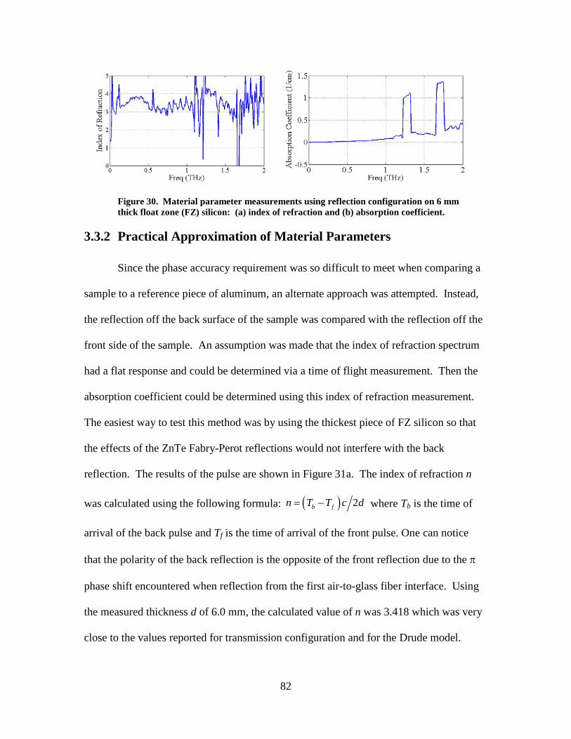
82
Figure 30. Material parameter measurements using reflection configuration on 6 mm thick float zone (FZ) silicon: (a) index of refraction and (b) absorption coefficient.
3.3.2 Practical Approximation of Material Parameters
Since the phase accuracy requirement was so difficult to meet when comparing a
sample to a reference piece of aluminum, an alternate approach was attempted. Instead,
the reflection off the back surface of the sample was compared with the reflection off the
front side of the sample. An assumption was made that the index of refraction spectrum
had a flat response and could be determined via a time of flight measurement. Then the
absorption coefficient could be determined using this index of refraction measurement.
The easiest way to test this method was by using the thickest piece of FZ silicon so that
the effects of the ZnTe Fabry-Perot reflections would not interfere with the back
reflection. The results of the pulse are shown in Figure 31a. The index of refraction n
was calculated using the following formula: ( ) 2b fn T T c d= − where Tb is the time of
arrival of the back pulse and Tf is the time of arrival of the front pulse. One can notice
that the polarity of the back reflection is the opposite of the front reflection due to the π
phase shift encountered when reflection from the first air-to-glass fiber interface. Using
the measured thickness d of 6.0 mm, the calculated value of n was 3.418 which was very
close to the values reported for transmission configuration and for the Drude model.

83
Figure 31. THz TDS reflection setup for thick FZ silicon: (a) pulses off front and back surface and (b) absorption coefficient using Fourier transform from each pulse.
Since the pulses were sufficiently separated in time, one could split the 200 psec
time period in half, and take the Fourier transform of each half. The absorption
coefficient is then calculated like in transmission setup, except that the Fresnel reflections
are different. A diagram showing the geometry of the Fresnel reflections in reflection
setup is shown in Figure 32. The following equation shows how to determine the
absorption coefficient α from the two reflected pulses:
( )( )
( ) ( )2 ln sam
sam ref
Ed R E
ωα ω
ω ω
= −
. (81)
The term ( )R ω is defined based on the geometry in Figure 32 as
( ) ( ) ( ) ( )( )
12 1 21 1 23 1
12 1
t t rR
rθ θ θ
ωθ
= (82)
where the coefficients are defined according to
( ) ( )( ) ( )
1 1 2 212 12 12
1 1 2 2
cos cos, 1
cos cosn n
r t rn n
θ θθ θ
−= = +
+ and (83)
( ) ( )( ) ( )
2 2 3 323 21 21
2 2 3 3
cos cos, 1
cos cosn n
r t rn n
θ θθ θ
−= = +
+ . (84)

84
The absorption coefficient could then be calculated as shown in Figure 32b. It remained
close to 0 cm-1 and shows some similarities to the transmission configuration graph.
d
θ1Einitial
r12
ESample
t12
t21
θ2
EFP REF
r23
Figure 32. Diagram showing the geometry of the first Fabry-Perot reflection from the sample in reflection configuration.
3.3.3 Other Material Parameter Measurements
In the previous two sections, the thick piece of FZ silicon, with a significant time
separation before the first FP reflection, was used to test two methods of extracting
material measurements using a THz TDS reflection configuration. In this section,
material parameter measurements were attempted on the high resistivity silicon and
finally on the glass fiber in an effort to find a useable reflection technique.
The first material analysis was performed on the high resistivity silicon. Figure
33 shows the THz (a) pulse return and the (b) spectrum with the effects of the Fabry-
Perot reflections from both the sample and the ZnTe. This made it difficult to determine
the index of refraction from Equation 78. To determine the material parameters, the first

85
(a) (b)
(c) (d)
(e)
Figure 33. THz TDS reflection (a) pulse and (b) spectrum for 1.016 mm high resistivity silicon. Isolation of the (c) front reflected pulse and the (d) back side reflected pulse in the time domain. The (e) absorption coefficient for high resistivity silicon measured using the spectrum of the front and back pulse.
technique that was attempted was to measure the index of refraction with the time delay
of the THz pulse between the front and back reflections. The index was measured to be

86
3.405 from either the peak of the pulse or the zero crossing. In order to measure the
absorption coefficient, a separate Fourier transform would have to be taken for both the
front and the back reflection. First, the front pulse was multiplied by the factor from
Equation 82 (-0.686) and then subtracted from the back reflection shown in 33c. Then
the reference pulse was multiplied by the Fresnel reflection coefficient (0.546) and
subtracted from the front reflected pulse for 33d. The Fourier transform of each was
taken and the result is shown in 33e. The result oscillates about zero from 0.1 - 1.2 THz.
The material measured next was the glass fiber composite without an exterior
coating. The glass fiber was unique from the silicon samples in that it had a considerably
higher absorption. The THz pulse in Figure 34a data was taken with the TDS reflection
setup. A first attempt was made to measure the index of refraction using the timing
between the front and back reflections, however, the index measurements were lower
than in transmission configuration. An alternate method was tried using the relative
amplitude of the pulses measured peak-to-peak. The amplitude of the first glass fiber
pulse (1.5133) to the aluminum reference pulse (4.2124) was measured to be 0.3592.
Using the equation for the Fresnel reflection coefficient from the front surface, the index
of refraction was calculated to be 2.03 ± 0.02. With this index of refraction, the
absorption coefficient was calculated using the method outlined in section 3.3.2. The
graph in 34b shows the Fabry-Perot etalon effect in the glass fiber, while the graph in 34c
is filtered using a windowing technique. The coefficient was measured to be 7 ± 2 cm-1
at 0.5 THz and 18 ± 2 cm-1 at 1.0 THz which were close to the results for transmission.
The measurement appears to run out of dynamic range at approximately 1.0 THz, which
makes it slightly worse than transmission which was at about 1.25 THz.

87
(a) (b)
(c)
Figure 34. Plot of the (a) THz pulses reflected from the front and back of a glass fiber coupon. Absorption coefficient for the glass fiber (b) without filtering and (c) with filtering.
3.4 Burn Diagnostics Using THz TDS
One of the problems with designing aircraft is that the heat from jet engines can
cause damage to the external structure of the aircraft. THz TDS could be used to
measure the material properties of the aircraft glass fiber composites to determine if the
composition of the material has fundamentally changed. Polyimide is a resin which has
the characteristic of being very resilient to thermal loads, maintaining its properties for
long periods of continuous use at 230°C, and for short excursions as high as 480°C.

88
Composite samples were prepared that were heated with various temperatures close to the
maximum for polyimide for short durations.
3.4.1 Transmission Mode
One of the first steps that was taken in the nondestructive evaluation of damaged
samples was to consider whether the material properties were altered in any way by the
damage. Since the samples with heat damage on them were different than the previously
measured glass fiber samples in Figure 19, we measured the THz pulse and amplitude
spectrum for the sample and reference shown in Figure 35a and 35b. These damage
samples had a coating applied to the exterior of the glass fiber which changed the
properties slightly. The index of refraction for the unaltered composite remained
Figure 35. THz TDS (a) pulse and (b) amplitude spectra for air reference and coated glass fiber. (c) Index of refraction and (d) absorption coefficient measurements for coated glass fiber in the THz frequency range.

89
relatively constant in the THz frequency range at 2.05 ± 0.01 in 35c while the absorption
coefficient was measured as 17.5 ± 0.8 cm-1 (0.5 THz), 27.5 ± 0.8 cm-1 (0.8 THz) and 38
± 0.8 cm-1 (1 THz) shown in 35d. This is comparable to another measurement made on
glass fiber samples, where the index of refraction was 2.05-2.1 and the absorption
coefficient was 12 cm-1 (0.5 THz) and 26- 32 cm-1 (0.8 THz) [4].
Using the setup shown in Figure 40, we measured an undamaged glass fiber
sample followed by a series of damaged samples with heat damage. Thickness
measurements were made on each of the samples and their burn areas, where the most
visually noticeable difference was in the largest burn area (440°C for 4 minutes). Using
the measured thickness of each blistered area, we obtained the results in Figure 36 for the
(a) index of refraction and (b) absorption coefficient. Figure 36 shows that there is a
variation based on the thickness of the sample blister.
For comparison, the burned material parameter measurements were calculated
with the undamaged sample thickness, such that the optical path length through each
damage spot was constant. As is shown in Figure 37, two of the burn areas have
Figure 36. THz TDS material parameter measurements using actual thickness measurements for burn damage areas showing (a) indices of refraction and (b) absorption coefficients.

90
relatively the same optical path length as the undamaged area. The third damage area,
burned at 430°C for 6 minutes, may have been different due to a small difference within
the burn spot. There is an area in the center of the burn spot where there appears to be
either a removal of the outer coating or a residue created during the burning process.
Since it is in the center of the small burn spot it was not possible to ensure a THz TDS
measurement could be made outside of the difference area. These measurements suggest
that burning the samples at these high temperatures does not alter the material
parameters, but merely introduces a blistering of the glass fiber and/or coating.
Figure 37. THz TDS material parameter measurements, assuming the same thickness, for burn damage areas showing (a) indices of refraction and (b) absorption coefficients.
3.4.2 Reflection Mode
Reflection configuration could also potentially be used for material parameter
burn diagnostics on composites. A reflection technique would assume that the back side
reflection of the THz would be large enough to use the technique described in section
3.3.3. However, an exterior coating was present on all three of burn spots available for
this research, and this prevented most of the back reflection from being detected. A
comparison of a reflected pulse from glass fiber both with and without the coating is

91
shown in Figure 38. Nearly double the amplitude is reflected from the coated sample due
to the two reflections at the coating and composite surfaces. A very small back side
reflection is evident in 38a for the coated sample. A burned area of the glass fiber
without a coating would be required to test this technique.
Figure 38. Comparison of the reflected signal from a coated and uncoated sample, showing the (a) time domain and (b) frequency spectrum returns.
92
4. THz Imaging for Nondestructive Evaluation
This chapter explains the results and analysis of imaging using THz TDS for the
nondestructive evaluation of composites. It is divided primarily into a section on
transmissive imaging and another section on reflection imaging. However, prior to
analyzing the imaging results, there is an explanation of the samples and the setup,
including sections on the numerical modeling and measurements of the THz beam at the
sample position. Using each of the two imaging techniques, two-dimensional imaging
was performed on the test samples. Finally, the last portion of each technique described
the analysis of the depth of delaminations using THz TDS.
4.1 Sample Preparation
The composite samples that were provided by AFRL/RXLP to test representative
forms of exterior aircraft damage are shown in Figure 39. The samples that were heated
with various temperatures for short durations are labeled 2 and 3 in Figure 39. The first
sample was burned at 440°C for 4 minutes, creating a blister on the sample about 2 cm X
1.5 cm. The second sample was burned in two places: 430°C for 6 minutes and 425°C
for 20 minutes.
Another goal was to determine if various forms of damage could be imaged with a
THz TDS system in either transmission or reflection setup. Three additional samples
were prepared to test the ability of a THz TDS system to detect the damage. The first
composite specimen, labeled 1 in Figure 39, was used as a thickness standard coupon to
test the response of THz TDS imaging techniques to various sample thicknesses.

93
1 2 43 5
Burn Spots
0.92 mm
0.69 mm
0.46 mm
0.23 mm
Bend Axis
HiddenDefects
Figure 39. Photograph showing the 5 glass fiber samples: (1) thickness calibration sample, (2) & (3) burn samples, (4) mechanical stress sample, and (5) hidden defect sample showing the hidden location of two of the eight defects.
Another coupon, labeled 5, was prepared to search for flaws. This coupon consisted of
two laminated pieces and is described in another reference [50]. The bottom piece was
prepared by etching four layers and then creating a 6 mm slit and a 3 mm flat bottom hole
(~70 µm depth) in each of the four layers. A top layer was created by etching 4 layers
with the same thicknesses and then attaching to the bottom layer in the opposite direction
with epoxy, being careful not to allow any epoxy into the flaws. Finally, a third sample,
labeled 4 in Figure 39, was prepared by bending a piece of glass fiber about a fixed axis a
total of 6240 cycles to investigate mechanical damage with THz TDS imaging.
4.2 Transmission Mode Setup
The setup that was used for the THz TDS nondestructive evaluation and imaging
is illustrated in Figure 40. A photoconductive switch was used for the THz emitter and

94
an electro-optic crystal (ZnTe) was used for the detector. This setup differed from the
one used for material parameter measurement in that it used four off-axis parabolic
mirrors to steer the THz beam, focusing it tightly at the sample. The first and last
parabolic mirror had a diameter and focal length of 25 mm while the center two parabolic
mirrors had a focal length and diameter of 50 mm.
Figure 40. THz TDS Setup for Imaging Composites in Transmission Mode.
4.3 THz Beam Propagation and Modeling
This section shows the results of modeling a THz beam spatially as a Gaussian
through our THz TDS system and the minimization of the spot size at the sample. The
numerical results are presented for both the transmission and reflection configurations.
Finally, actual THz spot size measurements are compared to the modeling predictions.
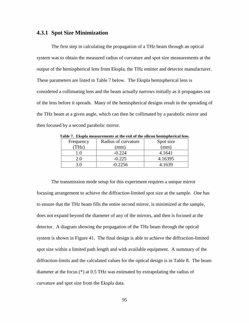
95
4.3.1 Spot Size Minimization
The first step in calculating the propagation of a THz beam through an optical
system was to obtain the measured radius of curvature and spot size measurements at the
output of the hemispherical lens from Ekspla, the THz emitter and detector manufacturer.
These parameters are listed in Table 7 below. The Ekspla hemispherical lens is
considered a collimating lens and the beam actually narrows initially as it propagates out
of the lens before it spreads. Many of the hemispherical designs result in the spreading of
the THz beam at a given angle, which can then be collimated by a parabolic mirror and
then focused by a second parabolic mirror.
Table 7. Ekspla measurements at the exit of the silicon hemispherical lens. Frequency
(THz) Radius of curvature
(mm) Spot size
(mm) 1.0 -0.224 4.1641 2.0 -0.225 4.16395 3.0 -0.2256 4.1639
The transmission mode setup for this experiment requires a unique mirror
focusing arrangement to achieve the diffraction-limited spot size at the sample. One has
to ensure that the THz beam fills the entire second mirror, is minimized at the sample,
does not expand beyond the diameter of any of the mirrors, and then is focused at the
detector. A diagram showing the propagation of the THz beam through the optical
system is shown in Figure 41. The final design is able to achieve the diffraction-limited
spot size within a limited path length and with available equipment. A summary of the
diffraction-limits and the calculated values for the optical design is in Table 8. The beam
diameter at the focus (*) at 0.5 THz was estimated by extrapolating the radius of
curvature and spot size from the Ekspla data.

96
0.1 0 0.1 0.2 0.3 0.4 0.5 0.6 0.7 0.80.025
0.013
0
0.013
0.025
Distance from THz Emit ter (meters)
Spot
size r
adius
(mete
rs)0.025
0.025−
W2 x( )
W2 x( )−
W3 x1( )
W3 x1( )−
W4 x2( )
W4 x2( )−
W5 x3( )
W5 x3( )−
W6 x4( )
W6 x4( )−
0.80.1− d1
x
d1
x, x1 d1+, x1 d1+, x2 d5+, x2 d5+, x3 d6+, x3 d6+, x4 d7+, x4 d7+,
Emitter Detector
Sample
Distance from THz Emitter (m)
THz
Bea
m S
pot S
ize
(m)
-0.0
250.
00.
025
-0.1 0.0 0.1 0.2 0.3 0.4 0.5 0.6 0.7 0.8
f = 25 mmd = 25 mm
f = 50 mmd = 50 mm
f = 25 mmd = 25 mm
f = 50 mmd = 50 mm
Figure 41. Diagram showing the transmission optical system with THz beam focusing on sample at 1 THz.
Table 8. Comparison of diffraction-limited spot sizes with THz beam optical design focus spot sizes for the transmission configuration.
Frequency (THz)
Diffraction-Limited Beam Diameter (μm)
THz Beam Diameter at Focus for Design (μm)
0.5 1200 1181* 1.0 600 617 2.0 300 312 3.0 200 209
A similar analysis can be performed to design the optical system for a THz TDS
reflective configuration. The goal of that design is to minimize the spot size at the
sample with available equipment within the shortest path length. Using the Ekspla data
from Table 7, one can design an optical system in which five parabolic mirrors are used
to steer the THz beam as shown in Figure 42. The maximum diameter of the THz beam
at the third parabolic mirror is 31 mm, limiting the focusing ability of the system. The
diffraction-limited spot size and the calculated Gaussian beam size at the sample are
shown in Table 9.

97
Distance from THz Emit ter (meters)
THz B
eam Di
amete
r (mete
rs)0.02
0.02−
W2 x( )
W2 x( )−
W3 x1( )
W3 x1( )−
W4 x2( )
W4 x2( )−
W5 x3( )
W5 x3( )−
W6 x4( )
W6 x4( )−
W7 x5( )
W7 x5( )−
W8 x6( )
W8 x6( )−
0.80.1− d1
x
d1
x, x1 d1+, x1 d1+, x2 d8+, x2 d8+, x3 d9+, x3 d9+, x4 d10+, x4 d10+, x5 d11+, x5 d11+, x6 d12+, x6 d12+,
Emitter Detector
Sample
-0.1 0 0.1 0.2 0.3 0.4 0.5 0.6 0.7 0.8
Distance from THz Emitter (m)
THz
Bea
m S
pot S
ize
(m)
-0.0
2
0
.0
0
.02
f = 25 mmd = 25 mm
f = 100 mmd = 50 mm
f = 100 mmd = 50 mm
f = 100 mmd = 50 mm
f = 100 mmd = 50 mm
Figure 42. Diagram showing the reflection optical system with THz beam focusing on sample at 1 THz.
Table 9. Comparison of diffraction-limited spot sizes with THz beam optical design focus spot sizes for the reflection configuration.
Frequency (THz)
Diffraction-Limited Beam Diameter (mm)
THz Beam Diameter at Focus for Design (mm)
0.5 2.42 2.48* 1.0 1.21 1.27 2.0 0.60 0.69 3.0 0.40 0.52
4.3.2 THz Beam Measurements
The next task was to build and align the THz TDS setup similar to the numerical
calculations, tweaking the parabolic mirrors and hemispherical mirrors to minimize the
spot size. Although the final setup did not follow the model exactly, it provided a good
starting point. The first setup that was measured for spot size at the sample was the
transmission configuration. The first technique that was used was the knife edge method,
scanning a knife blade through the THz beam horizontally and vertically. The knife was

98
scanned through the beam from 0% blockage to 100% blockage and beamwidth was
measured between 88% of peak voltage and 12 % of peak voltage of an unobstructed
beam with the electro optic detector [21]. The smallest beam measurements were 1.65
mm in the horizontal direction and 2.38 mm in the vertical direction, making it elliptical
in nature. A circular hole of roughly 1.5 mm in diameter was then moved into the
position of the minimum beam size. The result was that approximately 90% of the peak
pulse voltage was transmitted through the hole.
Before imaging the composites in reflection configuration, the spot size was
measured again. The same knife edge technique was attempted in reflection
configuration, except that the knife was used to reflect the THz and not block it. In the
horizontal direction, a spot width of 3.0 mm was obtained, while a spot width of 2.75 mm
was obtained for the vertical direction. The positioning of the knife was more difficult in
reflection setup so another method was attempted. This second method included the use
of the circular hole with a piece of aluminum behind the hole. The geometry of this setup
is shown in Figure 43 where θ is the angle of incidence, X is the diameter of the incident
THz beam, and Y is the spot size of the THz beam on the aluminum reflector. The
method of calculating the spot size on the sample (Y) was to close the pupil and the
measure the diameter at which 92% of the pulse peak was detected. The following
equation was used to determine the spot size (Y):
( )2 sinY D d θ= − (85)
where d = 5 mm. Given an incident angle of 20° and a measured pupil diameter of 7.2
mm, the spot size was calculated to be 3.78 mm. Since it was at an angle, the actual THz
beam width would be around 3.55 mm.

99
Pupil Diameter (D)Adjustable
Aluminum Reflector5 mm
θ
Y
Figure 43. Diagram showing the geometry of the incident and reflected beam off the apparatus for measuring the THz spot size in TDS reflection configuration.
4.4 Imaging of Composites with Transmission Setup
This section shows and explains the results for the first method of THz imaging
using the TDS transmission setup shown in Figure 40 to obtain the images. Although this
setup is not likely for maintenance operations, it provides insight into the capabilities and
limitations of THz TDS imaging in general. In the first part of this section, there is a
description of some of the results using thickness measurements and a comparison of
some image processing techniques. The next portion of the section shows the results of
THz TDS scans on various types of damage, including heat damage, bending damage,
and hidden defects. Finally, the last section shows a measurement analysis of the depth
of delaminations.
4.4.1 THz TDS Thickness Measurements
One area of interest for imaging is whether the characteristics of the pulse change
with different thicknesses and heat damaged areas of glass fiber material. Figure 44
shows how the THz pulse is not only reduced in amplitude through thicker samples, but

100
is also spread out in time as higher frequency components are attenuated more rapidly
than lower ones. The arrival time of the pulse is also longer due to a longer optical path
length through thicker materials. This illustrates how the THz TDS system could be used
to measure sample thickness and hence a simple phase technique could be used to image
composites for nondestructive evaluation.
Figure 44. Relative delay of THz pulses for various thicknesses of glass fiber sample, including those that were etched (*).
4.4.2 Image Processing Comparison
The image processing technique that was described in section 2.4.6 was tested on
a piece of glass fiber with a circle etched in it. The circle was 12.5 mm in diameter and
approximately 70 µm in depth. A series of images are shown in Figure 45, showing the
progression of techniques from the original 1 X 1 mm pixel image in a. Figure 45c
shows the image after zero-padding in the spatial frequency domain and Figure 45d
shows the additional of the MATLAB ‘interp’ function to further smooth out the image in
Figure 45c. Figure 45b was added to show the effect of the MATLAB ‘interp’ function
without the frequency domain interpolation. The image in Figure 45e is the equivalent of
viewing the original pixel image in (a) at 1/10 the original size.

101
Figure 45. THz image of a 12.5 mm diameter circle etched in glass fiber showing (a) the original 1X1 mm pixel image, (b) image after MATLAB ‘interp’ function, (c) image after zero-padding 10 times in the spatial frequency domain, and (d) final image after applying MATLAB ‘interp’ function to part (c). (e) Comparison of (c) with 1/10th scale pixel image.

102
One of the consequences of using the zero-padding approach was that certain
features, like sharp edges, caused a periodic modulation in the image. An example of this
effect can be seen in Figure 46a. The “checker board” pattern could be reduced by zero-
padding with fewer zeros and then using a Wiener filter on the image to reduce the
modulation as is shown in Figure 46b.
Figure 46. Image comparison showing the (a) the zero-padding technique (10 times) and the (b) zero-padding technique (4 times) with the addition of a Wiener filter.
4.4.3 2-D Imaging Results
The first sample was prepared to calibrate the system based on material thickness.
A THz image was taken of a 1 X 1 cm section of overlapping milled out areas with
different thicknesses. The image is shown in Figure 47 where (a) represents the peak
pulse amplitude and (b) shows the pulse position at each pixel of the sample shown in (c)
[48]. The decrease in amplitude of the pulse at the edges is a result of THz scattering
[48]. The periodic modulation in Figure 47b is a result of the interpolation technique to
smooth out the pixels and does not match the pattern of the glass weave within the
composite.

103
Similar images can be shown using the area under the curve from the amplitude
spectrum in the frequency domain. The image in Figure 48 shows pixels that represent
the sum of the amplitudes over the entire frequency spectrum that could penetrate the
glass fiber composite. It closely resembles the peak pulse amplitude image shown in
Figure 47a. The differing heights of the edges of the milled out areas causes a frequency
(c)
Figure 47. THz TDS transmission images showing a section of the glass fiber that had been milled to two different thicknesses using peak pulse amplitude (a) and peak pulse position (b) techniques. A picture of the scan area on the calibration sample (c).
dependence in the amplitude intensity. This can be seen in Figure 48 (b) and (c). The
upper left quadrant is about 0.92 mm lower than the right half while the lower left
quadrant is about 0.69 mm lower than the right half. The ridge between the two left
quadrants has a height difference of 0.23 mm. The THz spot size is wavelength

104
dependent and was spread across the milled ridges differently depending on the position
of the pixel during this raster scan. The lower amplitude areas represent the positioning
of the THz spot so that a majority of the radiation at that frequency was scattered.
Figure 48. THz images formed by summing the area under the curve of the amplitude spectrum within a given frequency range for each pixel: (a) 0.1 – 1.3 THz, (b) 0.5 – 0.7 THz, (c) 0.7 – 0.9 THz.
4.4.3.1 Imaging of Burn Damage
The next task was to image the burn samples. The results of the burn dot images
formed by the peak amplitude of the THz pulses are shown in Figure 49 with the visibly
burned areas within the circles. Figure 49a shows the sample that was burned at 440°C
for 4 minutes over ~ 2 X 1.5 cm area. It has a visibly noticeable bubble or blister on its
exterior which roughly corresponds with the blue area within the black oval.

105
Figure 49. THz TDS images and photos for three burn areas on glass fiber samples: (a), (d) 440°C for 4 minutes; (b), (e) 430°C for 6 minutes; and (c), (f) 425°C for 20 minutes.
(d)
(e)
(f)

106
Comparisons of the THz time domain signal of pixels from the burn area were made with
those from outside the burn area. A comparison is shown in Figure 50 contrasting a THz
signal from an undamaged portion of the sample to one from the center of the large burn
area (440°C for 4 minutes). There appeared to be time domain reflections in several of
the pixels within the burn area, showing evidence of air gaps, but without a consistent
pattern between pixels. These reflections caused a reduction in the peak pulse amplitude
based on the Fabry-Perot etalon effect from the air – composite interfaces, which reduces
the initial peak pulse, and because of scattering from the small air gaps and
discontinuities. In the frequency domain, there were no consistent spectral changes to the
THz signals through the burn areas.
Figure 50. THz TDS (a) pulse image and (b) amplitude spectra for undamaged glass fiber sample and for an area with burn damage (440°C for 4 minutes). (c) THz TDS amplitude image of high resistivity silicon.

107
The other two burn areas are shown in Figure 49b and 49c, neither of which
showed much visual evidence of blistering. The dark blue area within the circle in Figure
49b is roughly equivalent to the position of the residue or coating loss. Since the
absorption spectrum remained higher than the unburned sample, even when adjusted to
the same optical path length, it is more likely that the dark blue area is a form of residue.
The red circular dots in Figure 49c and less noticeable orange dots in Figure 49b
correspond to the white marker dots made on the samples to show the extent of the burn
area. The THz image of the damage area in Figure 49c was inconclusive in showing
evidence of burning.
During many of the transmission scans, the laser output power varied, and this
variation was not stabilized until after the laser optics were cleaned. To demonstrate this
variation, a scan was made of the thin wafer of high resistivity silicon. This scan can be
seen in Figure 50c showing the approximate color variation for the pulse amplitudes that
were demonstrated in 49c. The mean amplitude was measured at 1.306 mV while the
standard deviation was 0.017 mV (1.33%) and the maximum variation was ±4% from the
mean. Over the same scan period, the laser power varied by 3%, roughly matching the
pulse amplitude pattern shown in the image. If one considers that in Figure 49c that the
amplitude varied by more than ±7% across the image (not including the marker dots) then
one could say that the signal-to-noise of the transmission setup contributed to the image
variations, but was not the most significant factor.

108
4.4.3.2 Imaging of Bending Damage
An attempt was made to show damage caused by mechanical fatigue as a result of
6240 bending cycles. Visually, one could observe a thin area of discoloration on one side
of the glass fiber strip and one could see a small amount of cracking and buckling on the
back side. In Figure 51, the image of the sample shows an area of lesser amplitude
corresponding roughly to where the axis of bending occurred. Electrical tape, in the
shape of an ‘X’, was attached at the top of the image area for reference as shown in the
first photo in 51b. The second photo in 51c shows the location of cracking on buckling
on the back side of the sample that corresponds to the pattern in the THz image. The
(b)
(c)
(d)
Figure 51. THz TDS image showing bend damage across the central bend axis (a). Photographs of the (b) front side of the composite strip showing the scan area with the location of the taped ‘X’ and the (c) back side showing the location of the cracking and buckling and the hexagonal structure. (d) Ultrasound image of the bend damage.
(a)

109
cracking and buckling follows the hexagonal pattern faintly visible in the picture.
Finally, the image in 51d shows an ultrasound image of the same damage, showing the
same damage area and the electrical tape.
4.4.3.3 Imaging of Hidden Defects
Voids were also investigated, which simulated either manufacturing defects or
damage caused by stress over time. THz images are shown in Figure 52a and 52b for a
circular void (3 X 3 mm) and a crack or slit void (6 mm length) in 52c. For the circular
(d)
Figure 52. THz TDS images showing 3 mm diameter milled area hidden between two glass fiber strips using (a) peak pulse amplitude and (b) peak pulse position. Linear slit void (6 mm length) (c) also hidden between two strips of glass fiber. The final picture is an x-ray computed tomography scan of the laminated sample showing the hidden circular and slit voids in the sample.
110
void, a simple time domain amplitude or phase technique was sufficient to detect the
void. For the slit void, a specific frequency range was required to isolate the approximate
position, and was more difficult to isolate on multiple attempts [48]. The voids show an
area of reduced amplitude, most likely due to the multiple reflections from the
air/composite interface. A larger number of samples per area could be useful in isolating
this slit void in space by providing more complete coverage at the higher frequency
components. Another candidate would be to use a rotate the sample at 45° to the THz
polarization and then collect pulses with the detector at horizontal polarization and then
vertical polarization.
4.4.4 Depth of Delamination Analysis
The previous experiments demonstrated the imaging of voids in a two-
dimensional plane. An attempt was made to use THz TDS to isolate a void in the third
dimension of depth using the time domain. The goal was to use THz TDS to find Fabry-
Perot reflections in a delaminated area of the laminated sample (#5 in Figure 39) where
the epoxy had not adhered the two glass fiber strips. The THz scans are shown in Figure
53a, showing the THz pulse after it had transmitted through the adhered area and the
delaminated area. The autocorrelation was taken for each of the two pulses
independently of each other in the attempt to show the Fabry-Perot reflections in Figure
53b. Then the sample was flipped over and the process was repeated in the opposite
direction Figure 53c and 53d. The timing of the Fabry-Perot reflections was calculated
with 2FP ref gfT n l c− = where gfn is the index of the glass fiber and l is the thickness of a
delaminated piece. Given that the index of refraction is 2.05 and that the thickness of the
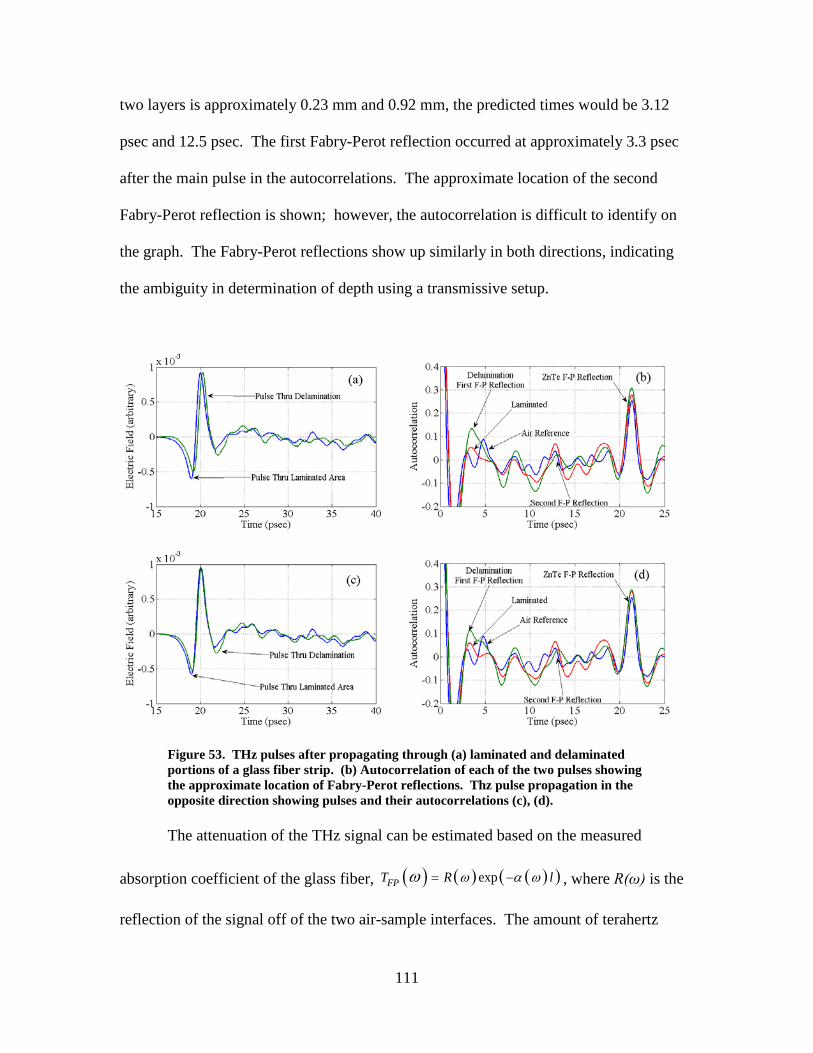
111
two layers is approximately 0.23 mm and 0.92 mm, the predicted times would be 3.12
psec and 12.5 psec. The first Fabry-Perot reflection occurred at approximately 3.3 psec
after the main pulse in the autocorrelations. The approximate location of the second
Fabry-Perot reflection is shown; however, the autocorrelation is difficult to identify on
the graph. The Fabry-Perot reflections show up similarly in both directions, indicating
the ambiguity in determination of depth using a transmissive setup.
Figure 53. THz pulses after propagating through (a) laminated and delaminated portions of a glass fiber strip. (b) Autocorrelation of each of the two pulses showing the approximate location of Fabry-Perot reflections. Thz pulse propagation in the opposite direction showing pulses and their autocorrelations (c), (d).
The attenuation of the THz signal can be estimated based on the measured
absorption coefficient of the glass fiber, ( ) ( ) ( )( )expFPT R lω α ωω = − , where R(ω) is the
reflection of the signal off of the two air-sample interfaces. The amount of terahertz

112
radiation, relative to the initial pulse, that is transmitted through the glass fiber composite
after undergoing a single Fabry-Perot reflection is shown in Figure 54, with a diagram of
the two pulses in 54a, calculations for TFP(ω) in 54b, and a picture of the 0.23 mm
delamination in 54c. One can observe in the figure that unless a delamination is very thin
(~ 0.23 mm) the reflection is unlikely to be recognizable above the system response.
r23
r21
Esam
EFP REF
Delamination
21 43 5
d
Figure 54. (a) Diagram showing the main pulse and the first Fabry-Perot reflection in transmission configuration. (b) A chart showing the relative amplitude of the first Fabry-Perot reflection to the main pulse after traveling through various thicknesses of composite. (c) A photograph showing the delamination.
(c)
(a)
(b)

113
4.5 Reflection Mode Imaging of Composites
This section shows the THz imaging results collected using the reflection setup
shown in Figure 29. The reflection configuration is a more likely technique for
maintenance than transmission. The samples were the same as those used for the
transmission setup, providing a direct comparison of the two techniques. This section
also looks at the same types of damage in two-dimensional imaging as well as a depth of
delamination analysis. Finally, results are shown for reflection scans on entire exterior
panels. All of the reflection mode images are taken with 1 X 1 mm step size in the raster
scan.
4.5.1 Thickness Calibration
A comparison of the thickness calibration sample imaged with a reflection setup
was compared to the transmission setup. The results of the peak pulse amplitude and
peak pulse position images are shown in Figure 55a and 55b. The resolution of the
images is not as good as the transmission images, but they still clearly show the three
distinct areas. The scattering of the THz signal is also shown in dark blue in Figure 55a
along the sharp edge between the different milled areas. The difference in amplitude in
each area is based on the geometry of the THz optical system and not based on any
characteristic of the glass fiber. The phase image in Figure 55b shows the opposite
pattern of the pulse arrival from the images for transmission configuration. Thicker
sections have a shorter arrival time in reflection, but a longer arrival time in transmission.
An additional scan was made by lengthening the pixel scan time from 25 psec to 40 psec
to ensure that the pulse reflected off the back side of the glass fiber was always collected.

114
From this data, a thickness image Figure 55c could be assembled using the optical path
length of the THz in glass fiber.
Figure 55. THz TDS reflection images showing a section of the glass fiber that had been milled to two different thicknesses using peak pulse amplitude (a) and peak pulse position (b) techniques. The final image (c) shows a thickness estimation for a separate scan.
4.5.2 2-D Imaging Results
The following section shows the image results for the various types of damage.
One of the issues that makes reflection mode imaging different from transmission setup is
that the tip and tilt of the sample can vary as the sample is moved through the THz beam.
This is caused by a slight angle misalignment (±2°) of the sample to the raster scanning
mechanism and/or a warping or curvature of the sample. This can create an artificial

115
delay of the pulse from top-to-bottom or from left-to-right. It can have the same effect on
the amplitude due to a changing of the geometric alignment of the reflected beam through
the collection optics. Linear correction techniques were implemented in post processing
to attempt to correct these deficiencies. The bandwidth of the signal reflected from the
surface was much greater than the bandwidth of any signal that penetrated the glass fiber
at any depth.
4.5.2.1 Imaging of Burn Damage
The burn damage was imaged using the reflection configuration on the three areas
analyzed earlier. The first burn area (440°C for 4 minutes), which had the most
noticeable blister, was imaged first and the amplitude and phase images are shown in
Figure 56. The rough area of the blister is encompassed by the oval. The amplitude
image shows the sensitivity of the geometry of the sample within the TDS setup. One
part of the bubble actually reflected more THz than the undamaged portion due to the
initial alignment with the upper right corner of the image. The angular dependence of the
reflection to the sample geometry causes a variation in the reflected amplitude due to a
changing alignment of the THz beam within the THz optics. The phase plot shows a
more accurate representation of the bubble where the true shape of the bubble is more
apparent.
One can also observe the pulse shape characteristics in each of the pixels. For
example, a pixel was chosen on the right side of the bubble and is shown in Figure 56c.
One can see the double reflection off the bubble surface and off a hidden delamination
below. The time of flight difference of 6.6 psec can be used to calculate the distance

116
between the pulses. Assuming an index of refraction of 2.05, the distance between the
reflections was 483 µm. The index is a rough estimate, because the bubble could contain
some combination of air, coating, and glass fiber. However, if this estimate is close, then
it would make sense that the delamination is close to where the original surface was
located. An x-ray image of the sample, showing the bubble from the side profile, can be
seen in Figure 56d.
Figure 56. THz TDS reflection images for burn damage from heating at 440°C for 4 minutes for (a) peak pulse amplitude and (b) peak pulse position. Pulse return from the right side of the bubble showing the double pulse return (c). X-ray computed tomography image showing a side profile of the large burn blister (d).
Additionally, one can determine the approximate height of the bubble by
measuring the difference in the pulse phase between the center of the burn area and the
unburned area. From the diagram, one could choose a pulse position of 13 psec at the
(d)

117
center of the bubble and another of approximately 16 psec from outside the bubble for a
difference of 3 psec. This equates to a height difference of 450 µm which is the
approximate thickness difference between the bubble (1.80 mm) and the undamaged
glass fiber (1.35 mm).
The sample with the other two burn spots was imaged next. First, the area that
had been heated at 430°C for 6 minutes was imaged and is shown in Figure 57a. Instead
of using the peak pulse amplitude, the minimum pulse amplitude was used since it
showed the residue coating better. This might have been due to the THz pulse reflecting
off both the exterior paint and the surface of the glass fiber, which could have flipped the
polarity of the pulse. The dot in the center of the circled burn spot corresponds with the
residue. Next, the area that was heated at 425°C for 20 minutes was imaged with the
reflection setup and is shown in Figure 57b. Like transmission mode, there was no hint
of damage to the glass fiber, however, the white marker dots showed up again quite well.
After adjusting the contrast, the apparent resolution of the dots is almost as precise as the
transmission setup images.
Figure 57. THz TDS reflection images showing the (a) minimum peak amplitude for burning at 430°C for 6 minutes and the (b) peak pulse amplitude for burning at 425°C for 20 minutes.

118
4.5.2.2 Imaging of Bending Damage
Next, the sample having the mechanical damage caused by bending the glass fiber
6240 cycles was imaged in reflection setup. The image is shown in Figure 58. There is
perhaps a slightly greater density of lower amplitude (1.2 – 1.4 THz) radiation around the
bend axis, but it is difficult to categorize as conclusive. Further attempts were made to
measure the thickness using a longer 40 psec scan time, but no additional detail was
obtained.
Figure 58. THz TDS reflection image using the amplitude of frequencies (1.2 – 1.4 THz) showing bend damage across the central bend axis.
4.5.2.3 Imaging of Hidden Defects
The laminated glass fiber coupon with hidden defects was imaged next. The 3
mm diameter circular void was scanned first and shown in Figure 59. Since the void was
hidden below the surface, a technique for imaging using the second THz pulse after the
main pulse was used instead. This was in an effort to measure the first Fabry-Perot
reflection located at the position of the adhesive and/or the air void. In this case the air

119
void had a larger index of refraction difference with the air than the glue, allowing it to
appear in the image. Attempts were made to show an image of the linear slit void, but
none of the techniques were successful in isolating its location.
Figure 59. THz TDS reflection image showing 3 mm diameter milled area hidden between two glass fiber strips using the amplitude of the Fabry-Perot reflection from the void.
4.5.2.4 Imaging and Analysis of Entire Panels
Up to this point, all of the THz imaging has been on thin coupons of glass fiber
with various forms of damage. On an aircraft, the glass fiber strips are attached to both
sides of a much thicker honeycomb structure and attached to the external part of the
aircraft. A THz TDS transmission scan was attempted on an entire panel (~3 cm thick),
however, very little of the energy penetrated through. Obviously, TDS reflection mode
would be required to detect damage in a panel. A couple of panels were prepared with
burn damage, holes, and paint remover on their surface for imaging and analysis with
THz radiation.
The first panel that was scanned had holes (4.5 mm diameter) punched through
the glass fiber representing puncture damage and it also had burn damage between the

120
holes. The scanned area of the panel included one hole and two burn areas. A very
noticeable burn area was on the right half. The other burn area was much less visibly
noticeable; in fact, I didn’t visibly notice it until it showed up on the THz TDS scan.
Images of the panel can be seen in Figure 60, where the (a) minimum peak amplitude, (b)
maximum peak position, and (c) amplitude spectrum (1.4 – 1.6 THz) are used to
construct the images. Finally, a plot of the time domain pulse reflected from an
undamaged, coated surface is compared to a pulse reflected from a partially uncoated,
blistered portion of the panel in 60d.
Figure 60. THz TDS reflection setup scan on entire panel with puncture hole (4.5 mm diameter) and two burn blisters. Images were constructed using the (a) minimum peak pulse amplitude, (b) maximum peak pulse position, and (c) the frequency spectrum amplitude added under the curve (1.4 – 1.6 THz). THz pulses reflected from coated surface and partially uncoated burn blister (d).

121
The next panel that was scanned had a solvent, called butanone, applied to the
exterior surface of the panel to dissolve away the paint. The area that was dissolved was
about 7 mm wide and can be seen on either of the images in Figure 61. One could also
estimate the thickness of the paint that was dissolved away if the index of refraction for
the paint coating was known.
Figure 61. THz images constructed using the (a) peak pulse amplitude and (b) peak pulse position of a panel with its coating dissolved away by butanone.
The two past panels show that THz TDS setup in reflection mode is capable of
imaging changes to the exterior of glass fiber on a panel. For this research there were no
samples available with known, hidden defects, but one could assume that hidden defects
would reflect THz energy in the same way that the thin glass fiber coupons would.
However, another important question was how the honeycomb structure under the glass
fiber reflects the THz signal. Long, time duration scans were taken of an entire panel to
see whether there were any reflections within the honeycomb. A typical plot of the first
half of a long scan is shown in Figure 62a where the time domain reflections off of a
coated and uncoated glass fiber surface are shown. Apart from the ZnTe etalon effect,
there is nothing remarkable about the pulse characteristics even when it was extended to

122
200 psec. Apparently, the honeycomb either traps the energy or it gets attenuated
sufficiently so that it is not detected. There is also no back reflection off of the back side
of the glass fiber, indicating a smooth transition from the glass fiber to the honeycomb.
A graph of the corresponding frequency spectra are shown in Figure 62b.
Figure 62. THz TDS (a) time domain plots and (b) frequency spectra for a coated and uncoated surface of an aircraft panel.
4.5.2.5 Paint Thickness Approximations
An observation that was noticed was that the coating on the glass fiber caused a
double reflection of the THz pulse on the front surface. A time domain plot of this can be
seen in Figure 63a where there is a double peak in the positive polarity of the pulse. It is
also apparent that the back reflection of the coated glass fiber sample is non-existent,
making any attempt to measure the material properties with the back pulse to be
impossible. A plot of the THz frequency spectrum is shown in 63b, where the spectrum
shows a fast roll-off after 0.4 THz and 1.6 THz due to the Fabry-Perot effect with the
paint. One could use the time domain plot to determine the thickness of the coating given
the index of refraction of the coating or vice versa. Since the index of refraction for the
coating was estimated to be around 2.05, the thickness of the coating on the glass fiber
samples was 55 µm.
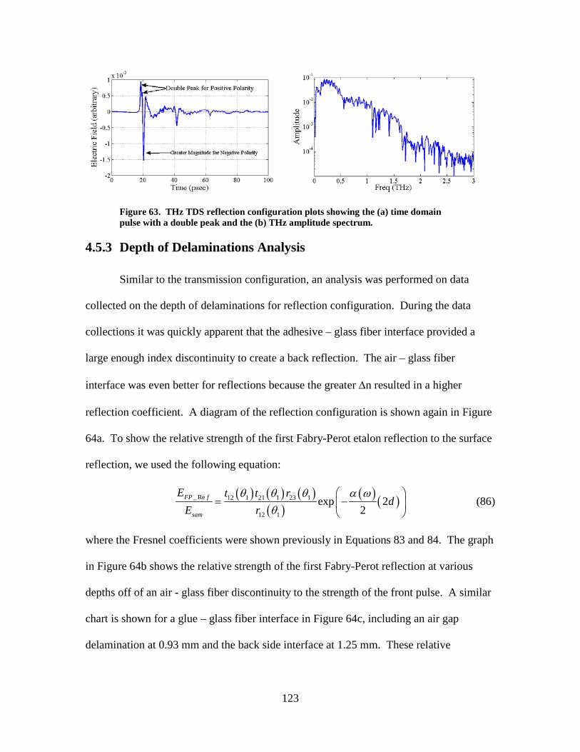
123
Figure 63. THz TDS reflection configuration plots showing the (a) time domain pulse with a double peak and the (b) THz amplitude spectrum.
4.5.3 Depth of Delaminations Analysis
Similar to the transmission configuration, an analysis was performed on data
collected on the depth of delaminations for reflection configuration. During the data
collections it was quickly apparent that the adhesive – glass fiber interface provided a
large enough index discontinuity to create a back reflection. The air – glass fiber
interface was even better for reflections because the greater ∆n resulted in a higher
reflection coefficient. A diagram of the reflection configuration is shown again in Figure
64a. To show the relative strength of the first Fabry-Perot etalon reflection to the surface
reflection, we used the following equation:
( ) ( ) ( )( )
( ) ( )_ Re 12 1 21 1 23 1
12 1
exp 22
FP f
sam
E t t rd
E rθ θ θ α ω
θ
= −
(86)
where the Fresnel coefficients were shown previously in Equations 83 and 84. The graph
in Figure 64b shows the relative strength of the first Fabry-Perot reflection at various
depths off of an air - glass fiber discontinuity to the strength of the front pulse. A similar
chart is shown for a glue – glass fiber interface in Figure 64c, including an air gap
delamination at 0.93 mm and the back side interface at 1.25 mm. These relative

124
amplitudes of the Fabry-Perot reflections compared favorably with the amplitudes of the
measured data from the laminate sample.
d
θ1
θEinitial
r12
ESample
t12
t21
θ2
EFP REF
r23
(a)
(b) (c)
Figure 64. (a) Diagram of a delaminated sample showing the first Fabry-Perot reflection in reflection configuration. (b) A chart showing the relative strength of the first Fabry-Perot reflection after traveling through various thicknesses of glass fiber composite before the delamination. (c) A chart showing the relative strength of the first Fabry-Perot reflection from discontinuities including both glue-glass fiber (G-GF) and air-glass fiber (A-GF).
The next step was to analyze data that was collected at the various depths.
Examples of TDS time domain scans in reflection mode are shown in Figure 65. The
scan in 65a shows the very distinct reflections that occur when the THz pulse reflects

125
from the delaminated air-glass fiber interface and also the back air – glass fiber interface.
The scan in 65b shows an example of a Fabry-Perot reflection from a glue – glass fiber
interface. Both discontinuities were located at 0.23 mm below the sample surface and the
back side reflection can also be seen in both.
Figure 65. THz TDS time domain plots showing reflections from discontinuities: (a) air and (b) adhesive.
The technique that was used for depth determination was to use a Fourier
deconvolution D(t) in the time domain instead of the autocorrelation used for
transmission mode. This is demonstrated in the following equation:
( ) ( )( )D t ifft fft E t= (87)
in which fft is the fast Fourier transform and ifft is the inverse fast Fourier transform. A
comparison of the returns from discontinuities at various depths is shown in Figure 66 a-
f. The dashed lines were added to show the similarity of the backside reflections in each
scan along with the pulse reflection from the ZnTe etalon effect. A separate calculation
was made to remove the TDS system effects from the deconvolution. This was
accomplished by making a separate measurement of the THz pulse reflection from
aluminum and then subtracting out the aluminum from the sample. This removed most
of the main pulse and the ZnTe reflection. A series of depth measurements can be seen in
Figure 66 g-l for the various thicknesses. Each series of plots was measured from a

126
Figure 66. Fourier deconvolution of the discontinuities present in a glass fiber sample laminated at various thicknesses: (a) 0.23 mm, (b) 0.46 mm, (c) 0.69 mm, (d) 0.92 mm, (e) 0.92 mm delaminated, and (f) no lamination. Fourier deconvolution with the TDS system characteristics subtracted are shown next. The various thicknesses were measured in the opposite direction: (g) 0.23 mm, (h) 0.23 mm delaminated, (i) 0.46 mm, (j) 0.69 mm, (k) 0.92 mm, and (l) no lamination.
Backside Reflection
ZnTe Reflection
Backside Reflection

127
different side of the sample, showing minimal difference from each side. A plot of the
calculated times and the autocorrelation times for the depth of delaminations measured
with transmission and reflection configuration is shown in Figure 67. The measured
autocorrelation time for transmission configuration is questionable beyond a
depth of 0.23 mm. Both of the techniques are capable of imaging defects on the order of
magnitude of a THz wavelength. A comparison of THz images between transmission
and reflection configuration is shown in Figure 67.
Figure 67. Comparison of the calculated time for F-P reflections through glass fiber to the measured autocorrelation values measured in both transmission and reflection configuration.

128
5. Conclusions and Recommendations
This chapter provides a summary of the research that was presented in the
previous chapters followed by directions for future research. It explains how THz TDS
has the potential to be a superior NDE technique for glass fiber composites over other
NDE techniques. It then compares and contrasts the advantages and disadvantages of the
TDS transmission or reflection setup. Finally, it provides recommendations for follow-
on research projects.
5.1 Major Research Contributions
This research was novel in a variety of different aspects. First, it is one of the first
research efforts that uses THz TDS as an NDE technique to inspect glass fiber aircraft
composite samples with representative forms of damage. Second, it demonstrates how to
use THz TDS to measure the material properties of a burn damage area on a composite in
an effort to determine if the material has been chemically altered. Third, it shows how
various types of surface and subsurface defects can be imaged and detected by either a
transmissive or reflective TDS configuration. Fourth, it also provides an analysis on how
effective each configuration would be at isolating the depth of discontinuities within the
composite. Finally, it also presents a technique for measuring material parameters in
reflection mode.
5.2 Conclusions
THz TDS has several potential advantages over other nondestructive evaluation
methods for inspection of aircraft glass fiber composites. Both ultrasound and eddy
129
current techniques require that the source and detector remain in contact with the aircraft.
In addition, eddy current testing requires that the material is conductive, which is not
applicable to glass fiber. X-ray techniques use ionizing radiation to penetrate the sample
which can cause safety issues for operators. X-rays can also require the use of penetrates
to help detect delaminations. Video inspection can be time consuming and prone to
human error. Microwaves have the ability to penetrate composites, but their resolution is
more limited due to their longer wavelengths. Infrared techniques can have better
resolution, but less penetration depth. THz can penetrate glass fiber without contacting it,
with submillimeter transverse resolution, and can detect surface defects, hidden voids,
delaminations, and bending damage in composites. The depth resolution for defects is
potentially much better than the transverse resolution, and thin composite samples can be
analyzed with THz TDS. Additionally, it can also be used to evaluate whether the
aircraft composite has been chemically altered from engine burn damage by measurement
of its index of refraction and absorption coefficient spectrum.
Material parameter measurements were made with both transmission setup and
reflection setup. The dielectric properties of low resistivity silicon wafers were modeled
with the Drude model and showed a close comparison with measured results. Fabry-
Perot etalon removal techniques were moderately effective in removing the oscillations
from the index of refraction and absorption spectra. It was more difficult to measure
material parameters with reflection configuration because the technique of comparing the
sample pulse to a reference pulse did not provide accurate results. For thicker samples, a
time domain separation of the front and back reflections provides a useful technique, if

130
one assumes a flat refractive index response. It becomes more difficult when the samples
are thinner and their absorption coefficients are higher.
Effective medium approximations were used to estimate the refractive index and
absorption coefficient spectrum of the glass weave after measuring the polyimide and
glass fiber composite separately. These indices of refraction were then used to calculate
the scattering properties of the composite and estimates of the scattering coefficient were
low for the THz spectrum due to the similarity of the indices of refraction for the two
composite materials and the density of inclusions.
An aircraft glass fiber composite with various forms of damage was examined
using both a transmissive and a reflective THz TDS system for NDE. Indices of
refraction and absorption coefficients in the terahertz frequency range were measured
using THz TDS in transmission configuration for comparison of damaged and
undamaged material states. Results showed that localized heat damage did not change
the material properties of the composite sample noticeably; however, changes in the
terahertz signal were observed due to material blistering and/or residue deposited. The
approximate depth of a delaminations could be determined in the time domain by
measuring the timing of a Fabry-Perot reflection through a thin slice of the composite.
Reflection configuration was much more effective in showing discontinuities, even
between an adhesive layer and the glass fiber. A hidden circular void was imaged and
there was also evidence that areas of damage from mechanical bending stress and
simulated hidden cracks could be detected with terahertz TDS imaging in both
configurations.

131
THz TDS in transmission setup was effective in locating voids at any depth or
thickness, but had difficulty in finding damage that was smaller than THz wavelengths.
Burn spots could be detected, but the dielectric properties of polyimide appeared to
remain unaltered at burn temperatures below 480°C. Additional burn tests at
temperatures approaching 480°C would have to be attempted to see if and when the
material properties of the composite would change. A THz TDS system in reflection
mode would be a more likely candidate for inspection of glass fiber composites on
aircraft and would likely be more effective in determining the depth of damage areas.
The glass fiber composite absorbs a significant amount of the THz radiation, attenuating
a transmission signal, and limiting the use of Fabry-Perot reflections for depth
measurements. In reflection mode, the magnitude of the first surface reflection and
subsequent reflections were more similar, which enabled a greater ability to locate the
depth of a void.
There were advantages and disadvantages to using either the TDS transmission or
reflection configuration. It was easier to get a smaller THz spot size onto the sample
using a transmission configuration. This was primarily due to the large ratio of focal
length to diameter in the parabolic mirrors and the cumbersome stages used to steer them.
Custom optical parts could alleviate this problem for reflection configurations.
Reflection mode is certainly a more likely candidate for a maintenance technique, as was
mentioned earlier, but transmission setup could aid in the design and quality control of
glass fiber composites. Reflection mode would also be a more effective technique in
determining the depth of delaminations. This is due to reflection mode signals traveling a
shorter distance through the attenuating glass fiber and due to the relative similarity in the

132
amplitude of Fresnel reflections between a void and the initial pulse. This can be easily
seen when one compares the results in Figure 64 to Figure 54, which is shown again as a
comparison in Figure 68. The relative amplitude of the first Fabry-Perot reflection is
calculated to be an order of magnitude larger in reflection configuration than in
transmission.
(a) (b)
Figure 68. Summary charts showing the relative amplitude of the first Fabry-Perot reflection to the main pulse after traveling through various thicknesses of glass fiber composite in (a) transmission configuration and (b) reflection configuration.
Finally, a comparison of the transmission and reflection configuration images are
shown next to a photograph of the damage sample in Figure 69. THz images are shown
for the hidden circular void, the calibration sample using both phase and amplitude
techniques, and the three burn damage areas.
5.3 Future Work
One of the areas of research that is currently on-going is to compare the results of
THz TDS on a set of glass fiber composites samples to other NDE techniques, such as
ultrasound, x-ray tomography, and thermography. This comparison could be very

133
Transmission Reflection
Hidden Circular Void
Thickness Calibration Phase
Thickness Calibration Amplitude
Figure 69. Comparison of various types of glass fiber damage/alterations between transmission and reflection configuration.

134
valuable in defining the potential strengths and weaknesses of using THz TDS for NDE
of glass fiber composites. THz TDS could also be investigated as an NDE technique for
two other types of composites: Kevlar and carbon fiber. The ability of THz to penetrate
carbon fiber would probably be limited due to its higher conductivity, but it could be
useful to determine the penetration depth and surface defects. Kevlar and glass fiber
samples, with various forms of damage, are also available from AFRL/RXLP.
Another task that could be performed in future research would be to calibrate the
absorption coefficient measurements with the THz TDS transmission setup. The
measurements on the absorption coefficient in this dissertation appeared to be
accurate, but did not explore coefficients much larger than 0 cm-1. The silicon wafer or
other semiconductor could be measured with THz TDS and compared to the Drude
Model prediction. For this dissertation, the only types of wafers that were obtained in
single quantities were those with a high resistivity. An attempt was made to find a
semiconductor with a higher doping level that could be purchased in small quantities
economically, but none could be located.
An area that could be explored in more detail would be the modeling of the THz
pulse shape. In the laboratory, the pulse shape characteristics could be changed
drastically by altering the position of any of the optics, including the parabolic mirrors
and hemispherical lenses, and the alignment of the pump or probe beam on either the
emitter or detector. One could characterize the effects that each of the parts of the THz
quasi-optical system has on the final pulse shape and frequency spectrum. One would
have to be able to isolate each component, vary the alignment, and measure the output.
These measurements could then be compared to a model of the THz Gaussian pulse

135
shape in space and time. Perhaps the most difficult items to characterize would be the
emitter and detector, and a special arrangement with their manufacturer may be required.
The analysis of the effective medium approximations could be expanded. A solid
piece of the glass used in the composite would have to be obtained so that it could be
accurately measured with the THz TDS transmission configuration. Then various
volume concentrations of the glass and polyimide could be mixed to form different
composite mixtures. The material properties of each composite mixture could then be
measured and compared directly to the effective medium approximations.
One of the quantitative NDE analyses used to assess the value of the technique is
to measure its resolution in detecting and identifying both surface and hidden damage.
Another area of future research would be to measure damage of various sizes, shapes, and
depths to define the limits of either a THz TDS transmission or reflection setup. The
THz spot size would have to be minimized in either case, using short focal length optics
and small translation stages. Samples would have to be prepared with defects that have
been carefully manufactured and measured, and with those defects varying in size from
the largest THz wavelengths down to a fraction of the smallest THz wavelengths.
Finally, the last area of suggested future research would be to design a setup in
reflection mode which could accurately measure the index of refraction and absorption
coefficient. The reflection technique that was used in this research was not robust or
precise enough to consistently measure material parameters accurately. One would have
to use an alignment system to ensure that the sample and reference were within 1 µm
across their entire reflected surface, if the setup in Figure 29 was used. An alternate
technique would be to use ellipsometry to measure the material properties in which no
136
reference measurement is needed. One would place a wire grid polarizer after the emitter
to split the THz into s- and p- polarizations followed by a wire grid analyzer before the
detector to detect the two polarizations with equal sensitivity. The sample would then be
placed at an angle near the Brewster angle for a good signal-to-noise ratio, the
ellipsometric angles measured and fitted, and the complex refractive index determined.

137
BIBLIOGRAPHY
1. Ahn, J. S., Kim, K. H., Noh, T. W., Riu, D., Boo, K., & Kim, H. (1995). Effective-medium theories for spheroidal particles randomly oriented on a plane: application to the optical properties of a SiC whisker-Al2O3 composite. Physical Review B (Condensed Matter), 52(21), 15244-52.
2. Altan, H., Huang, F., Federici, J. F., Lan, A., & Grebel, H. (2004). Optical and electronic characteristics of single walled carbon nanotubes and silicon nanoclusters by tetrahertz spectroscopy. Journal of Applied Physics, 96(11), 6685-9.
3. American Heritage Dictionary. Second College Edition. (1982). Boston: Houghton Mifflin Company.
4. Anastasi, R. F., & Madaras, E. I. (2005). Application of hilbert-huang transform for improved defect detection in terahertz NDE of shuttle tiles. Nondestructive Evaluation and Health Monitoring of Aerospace Materials, Composites, and Civil Infrastructure IV, 5767 356-362. from http://dx.doi.org/10.1117/12.600570
5. Anastasi, R. F., & Madaras, E. I. (2006). Terahertz NDE for metallic surface roughness evaluation. Nondestructive Evaluation and Health Monitoring of Aerospace Materials, Composites, and Civil Infrastructure V, 6176 61760. from http://dx.doi.org/10.1117/12.659463
6. Aspnes, D. (1985). The accurate determination of optical properties by ellipsometry. Handbook of Optical Constants of Solids, E. Palik, (ed.), Orlando: Academic Press, Inc.
7. Bartel, T., Gaal, P., Reimann, K., Woerner, M., & Elsaesser, T. (2005). Generation of single-cycle THz transients with high electric-field amplitudes. Optics Letters, 30(20), 2805-2807.
8. Baxter, J. & Schmuttenmaer, C. (2006). Conductivity of ZnO nanowires, nanoparticles, and thein films using time-resolved terahertz spectroscopy. Journal of Chemical Physics B, 110( 25229-25239).
9. Bakker, H. J., Cho, G. C., Kurz, H., Wu, Q., & Zhang, X. C. (1998). Distortion of terahertz pulses in electro-optic sampling. Journal of the Optical Society of America B, 15(6), 1795-1801.
10. Beard, M. C., Turner, G. M., & Schmuttenmaer, C. A. (2002). Terahertz spectroscopy. Journal of Physical Chemistry B, 106(29), 7146-7159.
11. Bolivar, P. H., Brucherseifer, M., Rivas, J. G., Gonzalo, R., Ederra, I., Reynolds, A. L., et al. (2003). Measurement of the dielectric constant and loss tangent of high

138
dielectric-constant materials at terahertz frequencies. IEEE Transactions on Microwave Theory and Techniques, 51(4), 1062-1066.
12. Chan, W., Deibel, J., Mittleman, D. (2007). Imaging with terahertz radiation. Reports on Progress in Physics, 70(8), 1325-1379.
13. Chau, K. J., Mujumdar, S., & Elezzabi, A. Y. (2005). Terahertz propagation in non-homogeneous strongly scattering media. Terahertz and Gigahertz Electronics and Photonics IV, 5727(1) 177-85. from http://dx.doi.org/10.1117/12.591279
14. Cheville, A., Zhang, X. C., Grischkowski, D., Reiten, M. T. (2007). THz Tutorial. CLEO 2007 THz Workshop.
15. Clancy, T., Pieczenik S., (1996). Games of State. New York: Penguin Putnam.
16. Cooney, A., & Blackshire, J. L. (2006). Advanced imaging of hidden damage under aircraft coatings. Advanced Sensor Technologies for Nondestructive Evaluation and Structural Health Monitoring II, 6179 617902. from http://dx.doi.org/10.1117/12.659035
17. Dai, J., Zhang, J., Zhang, W., & Grischkowski, D. (2004). Terahertz time-domain spectroscopy characterization of the far-infrared absorption and index of refraction of high-resistivity, float-zone silicon. Journal of the Optical Society of America B. 21(7), 1379-85.
18. Department of Defense. Military Handbook: Polymer Matrix Composites Utilization of Data. Mil-Hdbk-17-3D. Washington: GPO, 25 Feb 1994.
19. Diels, J. C., & Rudolph, W. (2006). Ultrashort Laser Pulse Phenomena. New York: Academic Press.
20. Dikmelik, Y., Spicer, J. B., Fitch, M. J., & Osiander, R. (2006). Effects of surface roughness on reflection spectra obtained by terahertz time-domain spectroscopy. Optics Letters, 31(24), 3653-5.
21. Dobroiu, A., Yamashita, M., Ohshima, Y., Morita, Y., Otani, C., & Kawase, K. (2004). Terahertz imaging system based on a backward-wave oscillator. Applied Optics. 5637-5646.
22. Dorney, T., Johnson, J., Mittleman, D., & Baraniuk, R. (2000). Imaging with THz pulses. Proceedings of 7th IEEE International Conference on Image Processing, 1 764-7. from http://dx.doi.org/10.1109/ICIP.2000.901071
23. Dorney, T. D., Baraniuk, R. G., & Mittleman, D. M. (2001). Material parameter estimation with terahertz time-domain spectroscopy. Journal of the Optical Society of America A (Optics, Image Science and Vision), 18(7), 1562-71.

139
24. Duvillaret, L., Garet, F., & Coutaz, J. L. (1999). Highly precise determination of optical constants and sample thickness in terahertz time-domain spectroscopy. Applied Optics, 38(2), 409-15.
25. Duvillaret, L., Garet, F., Coutaz, J. L., & Whitaker, J. F. (1997). A reliable method for the extraction of material parameters of thick and thin samples in THz time-domain spectroscopy. 13 (ISBN 1 55752 486 6), 248-51.
26. Ekspla. Laser Spectroscopy. (2007). Terahertz Spectroscopy Kit Brochure. Vilnius, Lithuania. http://www.ekspla.com/en/main/products/84?pid=525
27. Fletcher, J. R., Swift, G. P., Dai, D. C., Levitt, J. A., & Chamberlain, J. M. (2007). Propagation of terahertz radiation through random structures: An alternative theoretical approach and experimental validation. Journal of Applied Physics, 101(1), 013102.
28. Fletcher, J. R., Swift, G. P., Dai, D., & Chamberlain, J. M. (2007). Pulsed terahertz signal reconstruction. Journal of Applied Physics, 102(11), 113105-1.
29. Garcia-Vidal, F. J., Pitarke, J. M., & Pendry, J. B. (1997). Effective medium theory of the optical properties of aligned carbon nanotubes. Physical Review Letters, 78(22), 4289-92.
30. Gornov, E., Peiponen, K. E., Svirko, Y., Ino, Y., & Kuwata-Gonokami, M. (2006). Efficient dispersion relations for terahertz spectroscopy. Applied Physics Letters, 89(14), 142903-1.
31. Hoffmann, M. C., Yeh, K., Hwang, H. Y., Sosnowski, T. S., Prall, B. S., Hebling, J., & Nelson, K. A. (2008). Fiber laser pumped high average power single-cycle terahertz pulse source. Applied Physics Letters, 93(14), 141107-1.
32. Holst, G. C. (1998). Sampling, Aliasing, and Data Fidelity for Electronic Imaging Systems, Communications, and Data Acquisition. Winter Park, FL: JCD Publishing.
33. Hu, B. B., & Nuss, M. C. (1995). Imaging with terahertz waves. Optics Letters, 20(16), 1716-18.
34. Jackson, J. B., Mourou, M., Whitaker, J. F., Duling III, I. N., Williamson, S. L., Menu, M., & Mourou, G. A. (2007). Terahertz imaging for non-destructive evaluation of mural paintings. Optics Communications 281 527-532.
35. Jepsen, P. U., Fischer, B. M. (2005). Dynamic range in terahertz time-domain transmission and reflection spectroscopy. Optics Letters. 30(1). 29-31.
36. Jepsen, P. U., Jensen, J. K., & Moller, U. (2008). Characterization of aqueous alcohol solutions in bottles with thz reflection spectroscopy. Optics Express, 16(13), 9318-9331.

140
37. Jian, Z., & Mittleman, D. M. (2006). Characterization of guided resonances in photonic crystal slabs using terahertz time-domain spectroscopy. Journal of Applied Physics, 100(12), 123113-1.
38. Jian, Z., Pearce, J., & Mittleman, D. M. (2005). Two-dimensional photonic crystal slabs in parallel-plate metal waveguides studied with terahertz time-domain spectroscopy. Semiconductor Science and Technology, 20(7), 300-6.
39. Jian, Z., Pearce, J., & Mittleman, D. M. (2004). Defect modes in photonic crystal slabs studied using terahertz time-domain spectroscopy. Optics Letters, 29(17), 2067-2069.
40. Jordens, C., Koch, M. (2008). Detection of foreign bodies in chocolate with pulsed terahertz spectroscopy. Optical Engineering 47(3),037003-1.
41. Kang, C., Maeng, I. H., Oh, S. J., Lim, S. C., An, K. H., Lee, Y. H., et al. (2007). Terahertz optical and electrical properties of hydrogen-functionalized carbon nanotubes. Physical Review B (Condensed Matter and Materials Physics), 75(8), 85410-1.
42. Kerker, M. (1969). The Scattering of Light and other Electromagnetic Radiation. London: Academic Press.
43. Kubota, T., Talekar, P., Sudarshan, T. S., Ma, X., Parker, M., & Ma, Y. (2002). An automated defect detection system for silicon carbide wafers. IEEE SoutheastCon 2002, 42-47. from http://dx.doi.org/10.1109/SECON.2002.995555
44. Kuzel, P., Nemec, H., Kadlec, F., Duvillaret, L., & Coutaz, J. L. (2006). Independent determination of the complex refractive index and wave impedance by time-domain terahertz spectroscopy. Optics Communications, 260(1), 175-83.
45. Lee, S. (2008). Scattering by a dense layer of infinite cylinders at normal incidence. Journal of the Optical Society of America A, 25(5), 1022-1029.
46. Ma, X., Parker, M., & Sudarshan, T. S. (2002). Nondestructive defect delineation in SiC wafers based on an optical stress technique. Applied Physics Letters, 80(18), 3298-300.
47. Maeng, I., Kang, C., Oh, S. J., Son, J. H., An, K. H., & Lee, Y. H. (2007). Terahertz electrical and optical characteristics of double-walled carbon nanotubes and their comparison with single-walled carbon nanotubes. Applied Physics Letters, 90(5), 51914-1.
48. Mittleman, D. (2003). Terahertz imaging. Sensing with terahertz radiation. D. Mittleman (ed.), New York: Springer.

141
49. Myroshnychenko, V. & Brosseau, C. (2008). Effective complex permittivity of two-phase random composite media: a test of the two exponent phenomenological percolation equation. Journal of Applied Physics, 103(8), 084112-1.
50. Na, J. K. (2005). Ultrasonic inspection of thin high performance composite structures. Review of Progress in Quantitative Nondestructive Evaluation, 28, AIP Conference Proceedings.
51. Naftaly, M. & Miles, R. H. (2007). Terahertz time-domain spectroscopy of silicate glasses and the relationship to material properties. Journal of Applied Physics. 102(043517), 1-6.
52. Naftaly, M. & Miles, R. E. (2007). A method for removing etalon oscillations from thz time-domain spectra. Optics Communications, 280, 291-295.
53. Nemec, H., Kuzel, P., Garet, F., & Duvillaret, L. (2004). Time-domain terahertz study of defect formation in one-dimensional photonic crystals. Applied Optics, 43(9), 1965-1970.
54. Oh, S. J., Kang, C., Maeng, I., Son, J., Cho, N. K., Song, J. D., et al. (2007). Measurement of carrier concentration captured by InAs/GaAs quantum dots using terahertz time-domain spectroscopy. Applied Physics Letters, 90(13), 131906.
55. Pearce, J. & Mittleman, D. (2002). Scale model experimentation: using terahertz pulses to study light scattering. Physics in Medicine and Biology. 47, 3823-30.
56. Pearce, J., Jian, Z., & Mittleman, D. M. (2004). Propagation of terahertz pulses in random media. Philosophical Transactions of the Royal Society London, Series A (Mathematical, Physical and Engineering Sciences), 362(1815), 301-14.
57. Pearce, J., Jian, Z., & Mittleman, D. M. (2005). Bayesian approach to non-Gaussian field statistics for diffusive broadband terahertz pulses. Optics Letters. 30(21), 2843-5.
58. Pearce, J., Doyle, K., Jian, Z., Deibel, J., & Mittleman, D. M. (2006). Nonstationary time-domain statistics of multiply scattered broadband terhertz pulses. Journal of the Optical Society of America B, 23(8), 1506-10.
59. Piesiewicz, R., Kleine-Ostmann, T., Krumbholz, N., Mittleman, D., Koch, M., & Kurner, T. (2005). Terahertz characterisation of building materials. Electronics Letters, 41(18), 1002-4.
60. Piesiewicz, R., Jansen, C., Mittleman, D., Kleine-Ostman, T., Koch, M., Kurner, T. (2007). Scattering analysis for the modeling of thz communication systems. IEEE Transactions on Antennas and Propagation, 55(11), 3002-3009.

142
61. Pupeza, I., Wilk, R., & Koch, M. (2007). Highly accurate optical material parameter determination with THz time-domain spectroscopy. Optics Express, 15(7), 4335-4350.
62. Redo-Sanchez, A., Karpowicz, N., Xu, J., Zhang, X.C. (2006). Damage and defect inspection with terahertz waves. The 4th Annual Workshop on Ultrasonic and Advanced Methods for Nondestructive Testing and Material Characterization, 67-77. from
63. Reiten, M. T., Hess, L., & Cheville, R. A. (2006). Nondestructive evaluation of ceramic materials using terahertz impulse ranging. Advanced Sensor Technologies for Nondestructive Evaluation and Structural Health Monitoring II, 6179 617905. from
www.ndt.net
http://dx.doi.org/10.1117/12.657734
64. Rutz, F., Koch, M., Khare, S., & Moneke, M. (2005). Quality control of polymeric compounds using terahertz imaging. Terahertz and Gigahertz Electronics and Photonics IV, 5727(1) 115-22. from http://dx.doi.org/10.1117/12.590301
65. Rutz, F., Hasek, T., Koch, M., Richter, H., Ewert, U. (2006). Terahertz birefringence of liquid crystal polymers. Applied Physics Letters 89(22), 221911.
66. Rutz, F., Koch, M., Khare, S., Moneke, M., Richter, H., & Ewert, U. (2006). Terahertz quality control of polymeric products. International Journal of Infrared and Millimeter Waves, 27(4), 547-56.
67. Sakai, K. (2005). Terahertz optoelectronics. Berlin; Kobe: Springer; NiCT, National Institute of Information and Communications Technology.
68. Selig, H., Khazan, M., & Wilke, I. (2000). Optical properties of glasses and ceramics for terahertz-technology. 2000 Conference on Lasers and Electro-Optics Europe, 1. from http://dx.doi.org/10.1109/CLEOE.2000.909935
69. Sengupta, A., Bandyopadhyay, A., Bowden, B. F., Harrington, J. A., & Federici, J. F. (2006). Characterization of olefin copolymers using terahertz spectroscopy. Electronics Letters, 42(25), 1477-1479.
70. Seo, M. A., Lee, J. W., & Kim, D. S. (2006). Dielectric constant engineering with polymethylmethacrylate-graphite metastate composites in the terahertz region. Journal of Applied Physics, 99(6), 66103-1.
71. Shen, Y. C., Taday, P. F., Pepper, M. (2008). Elimination of scattering effects in spectral measurement of granulated materials using terahertz time domain spectroscopy. Jounal of Applied Physics, 92(5), 051103-1.
72. Siegman, A. M., (1986). Lasers. Stanford University: University Science Books.

143
73. Sze, S. M., (1985). Semiconductor Devices: Physics and Technology. Hoboken, NJ: John Wiley & Sons, Inc.
74. Tuncer, E., Bowler, N., & Youngs, I. J. (2006). Application of the spectral density function method to a composite system. Physica B, 373(2), 306-12.
75. Wang, S., & Zhang, X. C. (2004). Pulsed terahertz tomography. Journal of Physics D: Applied Physics, 37(4), 1-36.
76. Wietzke, S., Jansen, C., Rutz, F., Mittleman, D., Koch, M. (2007). Determination of additive content in polymeric compounds with terahertz time-domain spectroscopy. Polymer Testing, 26, 614-618.
77. Wietzke, S., Jordens, C., Krumbholz, N., Baudrit, B., Bastian, M., Koch, M. (2007). Terahertz imaging: a new non-destructive technique for the quality control of plastic weld joints. Journal of the European Optical Society, 2, 07013-1.
78. Wikipedia. http://en.wikipedia.org/wiki
79. Withayachumnankul, W., Ferguson, B., Rainsford, T., Mickan, S. P., & Abbott, D. (2005). Material parameter extraction for terahertz time-domain spectroscopy using fixed-point iteration. Photonic Materials, Devices, and Applications, 5840(1) 221-31. from http://dx.doi.org/10.1117/12.612946
80. Withayachumnankul, W., Ferguson, B., Rainsford, T., Mickan, S. P., & Abbott, D. (2005). Simple material parameter estimation via terahertz time-domain spectroscopy. Electronics Letters, 41(14), 800-1.
81. Wu, D.H., & Meyer, J.R. (2004). Terahertz emission, detection and military applications. Terahertz for Military and Security Applications II, 5411 187-195.
82. Xin, X., Altan, H., Saint, A., Matten, D., & Alfano, R. R. (2006). Terahertz absorption spectrum of para and ortho water vapors at different humidities at room termperature. Journal of Applied Physics, 100(9), 094905-1.
83. Xu, J., Plaxco, K. W., Allen, S. J. (2006). Absorption spectra of liquid water and aqueous buffers between 0.3 and 3.72 THz. The Journal of Chemical Physics. 124(036101), 1-3.
84. Xu, J., Zhong, H., Yuan, T., Xie, X., Wang, S., Zhang, X. C., et al. (2004). T-rays identify defects in insulating-materials. Conference on Lasers and Electro-Optics (CLEO), 1 2 pp. vol.1.
85. Xu, X., Wang, X., & Wang, L. (2006). Deviation of optical constants extracted in terahertz transmission spectroscopy. Applied Optics, 45(4), 648-652.

144
86. Yariv, A., & Yeh, P., (1984). Optical Waves in Crystals, Propagation and Control of Laser Radiation. Wiley-Interscience.
87. Yasui, T., Yasuda, T., Sawanaka, K., & Araki, T. (2005). Terahertz paintmeter for noncontact monitoring of thickness and drying progress in paint film. Applied Optics, 44(32), 6849-56.
88. You, D., Jones, R.R., Bucksbaum, P.H., & Dykaar, D.R., “Generation of High-Power Sub-Single-Cycle 500-Fs Electronmagnetic Pulses,” Optics Letters 18, 290-292 (1993).
89. Younossi, O., Kennedy, M., Graser, J.C., Military Airframe Costs: The Effects of Advanced Materials and Manufacturing Process. RAND Corporation, 2001.
90. Yuan, T., Liu, H. B., Xu, J. Z., Al-Douseri, F., Hu, Y., & Zhan, X. C. (2003). THz time-domain spectroscopy of atmosphere with different humidity. Terahertz for Military and Security Applications. Proceedings of SPIE. 5070, 28-57.
91. Zhang, J. & Grischkowski, D. (2004). Terahertz time-domain spectroscopy study of silica aerogels and adsorbed molecular vapors. Journal of Physical Chemistry B. 108, 18590-18600.
92. Zhong, H., Xu, J., Xie, X., Yuan, T., Reightler, R., Madaras, E., et al. (2005). Nondestructive defect identification with terahertz time-of-flight tomography. IEEE Sensors Journal, 5(2), 203-8.
93. Zimdars, D., White, J., Stuk, G., Chernovsky, A., Fichter, G., & Williamson, S. (2006). Large area terahertz imaging and non-destructive evaluation applications. The 4th Annual Workshop on Ultrasonic and Advanced Methods for Nondestructive Testing and Material Characterization, UMass Dartmouth, N. Dartmouth, MA.

145
Vita
Christopher D. Stoik graduated from Rice Lake High School in Rice Lake,
Wisconsin in 1989. He attended the United States Air Force Academy and graduated
with a BS Physics in 1993. He was immediately commissioned a second lieutenant in the
U.S. Air Force and attended the Air Force Institute of Technology (AFIT) at Wright
Patterson AFB, OH, receiving an MS Electrical Engineering in 1995. Lt Stoik then
moved to Offutt AFB, NE and joined the 513th Engineering and Test Squadron as an
electronic warfare reprogramming engineer for the B-1B. His unit was dissolved and
relocated to Eglin AFB, FL as the 36th Electronic Warfare Squadron in 1997, where he
continued producing operational electronic warfare mission data for the B-1 and B-2
defensive systems.
In 2000, Captain Stoik joined the Joint STARS program office at Hanscom AFB,
MA as the chief of the advanced technology section. He joined the AWACS program
office at Hanscom in 2002, becoming the chief of the advanced surveillance sensors
branch. In 2004, Major Stoik moved to Wright Patterson AFB, OH, where he joined
AFRL Sensors Directorate as the Signature Center Lead for the automatic target
recognition division. He returned to AFIT in 2005 to complete his PhD Physics.

REPORT DOCUMENTATION PAGE Form Approved OMB No. 074-0188
The public reporting burden for this collection of information is estimated to average 1 hour per response, including the time for reviewing instructions, searching existing data sources, gathering and maintaining the data needed, and completing and reviewing the collection of information. Send comments regarding this burden estimate or any other aspect of the collection of information, including suggestions for reducing this burden to Department of Defense, Washington Headquarters Services, Directorate for Information Operations and Reports (0704-0188), 1215 Jefferson Davis Highway, Suite 1204, Arlington, VA 22202-4302. Respondents should be aware that notwithstanding any other provision of law, no person shall be subject to an penalty for failing to comply with a collection of information if it does not display a currently valid OMB control number. PLEASE DO NOT RETURN YOUR FORM TO THE ABOVE ADDRESS. 1. REPORT DATE (DD-MM-YYYY) 12-10-2008
2. REPORT TYPE AFIT PhD Dissertation
3. DATES COVERED (From – To) 25 Aug 2005 – 28 Dec 2008
4. TITLE AND SUBTITLE Nondestructive Evaluation of Aircraft Composites Using Terahertz Time Domain Spectroscopy
5a. CONTRACT NUMBER
5b. GRANT NUMBER 5c. PROGRAM ELEMENT NUMBER
6. AUTHOR(S) Christopher D. Stoik, Lt Col, USAF
5d. PROJECT NUMBER 5e. TASK NUMBER
5f. WORK UNIT NUMBER
7. PERFORMING ORGANIZATION NAMES(S) AND ADDRESS(S) Air Force Institute of Technology Graduate School of Engineering and Management (AFIT/EN) 2950 Hobson Way Wright Patterson AFB OH 45433-7765
8. PERFORMING ORGANIZATION REPORT NUMBER AFIT/DS/ENP/09-D02
9. SPONSORING/MONITORING AGENCY NAME(S) AND ADDRESS(ES) James L. Blackshire, Ph.D. Nondestructive Evaluation Branch Air Force Research Laboratory Materials and Manufacturing Directorate Wright Patterson AFB, OH 45433-7750
10. SPONSOR/MONITOR’S ACRONYM(S) 11. SPONSOR/MONITOR’S REPORT NUMBER(S)
12. DISTRIBUTION/AVAILABILITY STATEMENT APPROVED FOR PUBLIC RELEASE; DISTRIBUTION UNLIMITED 13. SUPPLEMENTARY NOTES 14. ABSTRACT Terahertz (THz) time domain spectroscopy (TDS) was assessed as a nondestructive evaluation technique for aircraft composites. Material properties of glass fiber composite were measured using both transmission and reflection configuration. The interaction of THz with a glass fiber composite was then analyzed, including the effects of scattering, absorption, and the index of refraction, as well as effective medium approximations. THz TDS, in both transmission and reflection configuration, was used to study composite damage, including voids, delaminations, mechanical damage, and heat damage. Measurement of the material properties on samples with localized heat damage showed that burning did not change the refractive index or absorption coefficient noticeably; however, material blistering was detected. Voids were located by THz TDS transmission and reflection imaging using amplitude and phase techniques. The depth of delaminations was measured via the timing of Fabry-Perot reflections after the main pulse. Evidence of bending stress damage and simulated hidden cracks was also detected with terahertz imaging. 15. SUBJECT TERMS 16. SECURITY CLASSIFICATION OF:
17. LIMITATION OF ABSTRACT UU
18. NUMBER OF PAGES 161
19a. NAME OF RESPONSIBLE PERSON Matthew J. Bohn, Lt Col, USAF
REPORT U
ABSTRACT U
c. THIS PAGE U
19b. TELEPHONE NUMBER (Include area code) (937) 255-3636 x4573 [email protected]
Standard Form 298 (Rev: 8-98) Prescribed by ANSI Std. Z39-18