Geostatistical Analysis of Yield Monitor Data for Precision Agriculture

by

Moshood Agba Bakare

A thesis submitted in partial fulfillment of the requirements for the degree of

Master of Science

in

Plant Science

Department of Agricultural, Food and Nutritional Science University of Alberta

© Moshood Agba Bakare, 2015

ii

Abstract

It is long known that yield and other crop and soil characteristics vary across a farm field

with measurements in the neighborhood being more similar than those far apart. However, such

in-field spatial variability has been generally ignored because uniformity is required as a

convenient means of operating modern farm equipment for most farming practices such as crop

inputs and harvest. Moreover, until recently, the ability to detect and assess the in-field spatial

variability has been limited. The situation is now changing with the recent advent of geomatic

technologies such as yield monitors equipped with GPS on combine harvesters. The objective of

this research was the geostatistical analysis of data from one such technology (yield monitor

data). The focus was investigating the utility of multi-year yield monitor data from the same farm

field located in southern Alberta for identifying patterns and stability of spatial variability. In this

125 ha field, three crops were grown in four years: wheat (Triticum aestivum L.) in 2008, canola

(Brassica napus L.) in 2009, wheat in 2010 and barley (Hordeum vulgare L.) in 2011. Yield

readings were cleaned using Yield Editor version 2.0 and normalized to remove scaling effect

over different crops and years. The cleaned and normalized data were analyzed to fit three

variogram models (exponential, Gaussian, and spherical) that are commonly used in

geostatistical applications. The model fitting indicated that the similarity between yield readings

were best described by an exponential function of the distance separating the readings, but with

the similarity disappearing at different distances in all four crop years, ranging from 39.6 m

(2008) to 99.6 m (2009). The spatial stability of yield patterns over the years was measured by

Pearson’s correlations using interpolated yields mapped to a common grid. The apparent lack of

spatial stability over the years suggests that recommended inputs or farm-level decisions such as

variable rate applications cannot be based just on ‘eyeballing’ yield/soil maps from raw data at

iii

one farm in one year. Instead, these recommendations or decisions should be based on the maps

or information derived from predicted data at multiple farms/locations over multiple years under

tested, statistically sound spatial models for precise and profitable management of farm fields.

iv

Preface

Research conducted for this thesis was supported by Dr. Rong-Cai Yang who initiated

every part of this project. This research was financially supported by a research grant from

Alberta Crop Industry Development Fund (ACIDF#2011C021R) to Dr. Yang.

I was responsible for data quality checks, data analysis, interpretation of results from data

analysis, and manuscript composition. Steve Larocque of Beyond Agronomy provided the data

used in this research. Zhiqiu Hu was also very supportive with the analysis, and contributed to

the edit of R scripts in the manuscript.

v

Dedication

This thesis is dedicated to the blessed memory of my beloved parents in person of Alhaji

Bakare Alabi and Alhaja Hawau Alake Bakare. I also dedicate this thesis to my darling wife,

Khadijat Olanike Bakare and my children (Marzouq and Mardhiyah).

vi

Acknowledgements

I would like to express my profound gratitude to my advisor, Dr. Rong-Cai Yang, for the

opportunity given me to be his graduate student. This thesis would not have been completed

without his supervision, patience, motivation, and moral support. I would also like to thank Dr.

Ty Faechner for serving as my committee member and giving me insightful comments,

suggestions and advice on my manuscript. Finally, I would like to thank Dr. Miles Dyck and Dr.

Paul Stothard for taking time out of their busy schedule to serve as my external examiner and

committee chair.

My sincere appreciation also goes to Dr. Zhiqiu Hu, who as a group member, was always

willing to assist and give his best suggestion towards the success of this research work. Many

thanks to Steve Larocque of Beyond Agronomy for providing the data used in this research and

for his prompt response to my request by email. He provided some useful information needed for

implementing this research. My research would not have been possible without his assistance.

I am indebted to my wife, Khadijat Olanike Bakare, for her moral support, sacrifice and

assistance during my study. I would also like to give thanks to Dr. Peter Kulakow, brothers,

sisters, and friends. They were always supporting and encouraging me with their best wishes.

This research was financially supported by a research grant from Alberta Crop Industry

Development Fund (ACIDF#2011C021R) to Dr. Yang.

And above all, thanks to Almighty God for His infinite source of strength, wisdom,

guidance and inspiration, and for giving immeasurable blessings, for without Him this could not

be feasible.

vii

Table of Contents

List of Tables ................................................................................................................................. x

List of Figures ............................................................................................................................... xi

List of Abbreviations .................................................................................................................. xii

1 Introduction and Literature Review .................................................................................... 1

1.1 Introduction ...................................................................................................................... 1

1.2 Precision agriculture ......................................................................................................... 3

1.3 Geomatics-based technologies for precision agriculture ................................................. 4

1.3.1 Global Positioning System ........................................................................................ 5

1.3.2 Real-Time Kinematic ................................................................................................ 6

1.3.3 Guidance and navigation........................................................................................... 6

1.3.4 Field recording and mapping .................................................................................... 6

1.3.5 Crop scouting ............................................................................................................ 7

1.3.6 Geographic Information System ............................................................................... 7

1.4 Data sources for precision agriculture .............................................................................. 8

1.4.1 Remote sensing ......................................................................................................... 8

1.4.2 Electrical Conductivity (EC)................................................................................... 10

1.4.3 Topography ............................................................................................................. 12

1.4.4 Yield monitoring ..................................................................................................... 12

1.5 Geostatistics in precision agriculture ............................................................................. 14

1.6 Research Methodology ................................................................................................... 16

1.6.1 Data Acquisition ..................................................................................................... 16

1.6.2 Data Quality Control ............................................................................................... 16

1.6.3 Data Analysis .......................................................................................................... 17

1.7 Research goal and objectives ......................................................................................... 17

1.8 Outline of the thesis........................................................................................................ 17

1.9 Figures ............................................................................................................................ 19

2 Identifying patterns of spatial variability .......................................................................... 20

2.1 Introduction .................................................................................................................... 20

viii

2.2 Material and Methods..................................................................................................... 22

2.2.1 Field description and data collection ...................................................................... 22

2.2.2 Data filtering ........................................................................................................... 22

2.2.3 Preliminary statistical analysis ................................................................................ 23

2.2.4 Geostatistical analysis ............................................................................................. 24

2.2.5 R programs for geostatistical analysis .................................................................... 27

2.2.6 Goodness-of-fit and Cross validation ..................................................................... 29

2.3 Results ............................................................................................................................ 31

2.4 Discussion ...................................................................................................................... 33

2.5 Summary and Conclusion .............................................................................................. 36

2.6 Tables ............................................................................................................................. 37

2.7 Figures ............................................................................................................................ 41

2.8 Appendices ..................................................................................................................... 52

3 Assessment of spatial stability of crop yields .................................................................... 69

3.1 Introduction .................................................................................................................... 69

3.2 Materials and Methods ................................................................................................... 71

3.2.1 Data Standardization ............................................................................................... 71

3.2.2 Interpolation grid size ............................................................................................. 71

3.2.3 Spatial interpolation ................................................................................................ 71

3.2.4 Assessment of stability of yield patterns ................................................................ 73

3.3 Results ............................................................................................................................ 74

3.4 Discussion ...................................................................................................................... 76

3.5 Summary and Conclusions ............................................................................................. 78

3.6 Tables ............................................................................................................................. 79

3.7 Figures ............................................................................................................................ 81

3.8 Appendices ..................................................................................................................... 87

4 General Discussion and Conclusions ................................................................................. 90

4.1 Introduction .................................................................................................................... 90

4.2 Summary and conclusion ............................................................................................... 90

4.3 Implications of the study ................................................................................................ 92

ix

4.4 Limitations of the study and recommendations for future research ............................... 93

References .................................................................................................................................... 95

x

List of Tables

Table 2.1 Agronomic parameters and climatic data of the Skodopoles field for the

seedling period (May – September 15) of each cropping season. ............................. 37

Table 2.2 Error detected and removed by each filter type expressed as a percentage of total

observations. Individual error points may have been detected by multiple filters. ... 38

Table 2.3 Descriptions of data density for yield readings collected in four crop years. ............ 38

Table 2.4 Summary statistics of yield (Mg ha-1

) for raw and cleaned datasets. ........................ 39

Table 2.5 Assessment of goodness fit of three covariance models (exponential, Gaussian

and spherical) to empirical variograms in four crop years. ....................................... 39

Table 2.6 Cross validation diagnostic statistics measured for prediction accuracy of fitted

models. ....................................................................................................................... 40

Table 2.7 Estimates of model parameters of an isotropic exponential model for the data

in four crop years. ...................................................................................................... 40

Table 3.1 Summary statistics of yield values interpolated through the ordinary block

kriging method in four crop years. ............................................................................. 79

Table 3.2 Pearson’s correlation coefficients for interpolated yields between six pairs of

four crop years using interpolation by ordinary block kriging. ................................. 79

Table 3.3 Pearson’s correlation coefficients for interpolated yields between six pairs of the

four crop years using interpolation by inverse distance weighting. ........................... 80

Table 3.4 Weighted sum of square errors (SSErr) as a means of assessing goodness of fit

with three commonly used covariance models (exponential, Gaussian

and spherical) to empirical variograms based on interpolated yields obtained

by ordinary block kriging……………………………………………………………80

xi

List of Figures

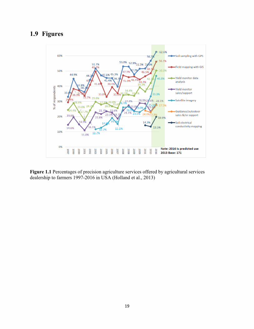
Figure 1.1 Percentages of precision agriculture services offered by agricultural services

dealership to farmers 1997-2016 in USA ................................................................ 19

Figure 2.1 A typical variogram plot showing the empirical semivariance over distance

classes (dots) and the fitted model (solid line). ....................................................... 41

Figure 2.2 Maps of raw yield readings collected for three crops grown in four years

(2008-2011). ............................................................................................................ 42

Figure 2.3 Maps of cleaned yield readings collected for three crops grown in four years

(2008-2011). ............................................................................................................ 43

Figure 2.4 Histograms with density curves and quantile-quantile plots of raw data

(a and b) and cleaned data (c and d) for wheat crop grown in 2008........................ 44

Figure 2.5 Histograms with density curves and quantile-quantile plots of raw data

(a and b) and cleaned data (c and d) of canola crop grown in 2009. ....................... 45

Figure 2.6 Histograms with density curves and quantile-quantile plots of raw data

(a and b) and cleaned data (c and d) of wheat crop grown in 2010. ........................ 46

Figure 2.7 Histograms with density curves and quantile-quantile plots of raw data

(a and b) and cleaned data (c and d) of wheat crop grown in 2011. ........................ 47

Figure 2.8 Variogram plot of wheat crop grown in 2008. ........................................................ 48

Figure 2.9 Variogram plot of canola crop grown in 2009. ...................................................... 49

Figure 2.10 Variogram plot of wheat crop grown in 2010. ........................................................ 50

Figure 2.11 Variogram plot of barley crop grown in 2011. ....................................................... 51

Figure 3.1 Spatial yield maps using ordinary block kriged predictions in four years

(2008-2011). ............................................................................................................ 81

Figure 3.2 Spatial yield maps of block predictions using the inverse distance weighting

(IDW) method for the three crops grown in four years (2008-2011). ..................... 82

Figure 3.3 Variogram plot of interpolated wheat crop yield grown in 2008. ........................... 83

Figure 3.4 Variogram plot of interpolated canola crop yield grown in 2009. .......................... 84

Figure 3.5 Variogram plot of interpolated wheat crop yield grown in 2010. ........................... 85

Figure 3.6 Variogram plot of interpolated barley crop yield grown in 2011. ........................... 86

xii

List of Abbreviations

EXP Exponential

GAU Gaussian

GIS Geographic information system

GPS Global positioning system

IDW Inverse Distance Weighting

Sec Seconds

Mph Miles per hour

NN Nearest Neighbour

bu/ac Bushels per acre

in Inches

SSErr Sum of squares error

ME Mean error

Mg/ha Mega gram per hectare

OK Ordinary Kriging

PA Precision Agriculture

REML Restricted maximum likelihood

SPH Spherical

SSCM Site-specific crop management system

VRT Variable rate technology

WGS84 World geodetic system 1984

1

1 Introduction and Literature Review

1.1 Introduction

The traditional practice of managing a farm field is characterized with uniform

application of crop inputs such as fertilization and pesticide applications across the entire field.

In the presence of in-field spatial variability, however, this practice would over-supply the inputs

in some parts of the field but under-supply the inputs in other parts. In this case, the blanket

application is not cost effective and it may also have adverse impacts on environments and agro-

ecology systems (Anselin et al., 2004; Pierce and Nowak, 1999). The spatial variability across

the field may be attributed to changes in soil attributes such as soil PH, soil texture, soil fertility,

water holding capacity, or other soil physical and chemical properties; cropping practices and

biological factors such as diseases and pests (Davidoff and Selim, 1988; Scharf and Alley, 1993;

Stroup et al., 1994; Webster, 2010; Wu and Dutilleul, 1999).

Precision agriculture (PA) is a farming management concept that stems from the need for

measurements and uses of in-field spatial and temporal variability in crops. Other terms such as

precision farming and site specific crop management (SSCM), are often used to mean the same

thing. The PA research aims at developing a decision support system for the whole-farm, thereby

optimizing returns on crop inputs while preserving resources (Basso et al., 2001; Booltink et al.,

2001; Hassall, 2009; McBratney et al., 2005). The PA research and management practices have

been driven largely by technological advances. The agricultural industry has benefited from

advances in geomatics-based technologies, including yield monitoring based on global

positioning system (GPS), geographical information system (GIS), variable rate technology

(VRT), miniaturized computer components, remote sensing, sensor devices, mobile computing,

soil electrical conductivity (EC), advanced information processing and telecommunications

(Bunge, 2014; Gibbons, 2000; Zhang et al., 2002). These technological advances have now

enabled the agricultural industry to gather massive, more comprehensive data on soil and crop

parameters which vary in space and time. The analysis of these massive georeferenced data is

statistically and computationally challenging but a number of approaches to the use such data for

practical SSCM include drawn yield maps, supervised and unsupervised classification

2

procedures on satellite or aerial imagery, and identification of yield stability patterns across

seasons (McBratney et al., 2005; Whelan et al., 1997). The benefits can be tangible such as

optimal input utilization and improved yield potential or intangible such as lessened operator

fatigue, better farm-level management decisions and reduced environmental impacts of

agriculture.

Crop producers are interested in the technology-driven PA research and practices because

the advent of new geomatics-based technologies enable them to create maps of the spatial

variability for many crop and soil variables that can be measured (crop yield, terrain features,

topography, organic matter content, moisture levels, nitrogen levels, pH, EC, Mg, K, etc.).

Further, these maps can be interpolated onto a common grid for a comparison across multiple

years (Kleinjan et al., 2007; Taylor et al., 2007). These measurements collectively help define

'recipe maps' which would be an important part of any generalized decision support system for

farm use.

One of the first technological advances that drove early PA research and practice was the

invention of yield meter by Massey Ferguson in 1982 (Oliver, 2010). The yield could be

measured on-the-go for the first time even though the observed data could not be mapped due to

lack of positional information. With the subsequent advent of GPS in the 1990s, the mapping of

soil and crop attributes became a common practice. Crops in a field-scale are now harvested

using a combine harvester equipped with GPS-based yield monitoring system. The quantity of

yield readings are massive and georeferenced within the field. Collecting such data at high

density is now a routine activity that is beyond the capability of traditional small-plot research.

The analysis of multiple spatially georeferenced observations within field represents a new

challenge to data analysts and field crop researchers (Eghball et al., 2003; Ferguson et al., 2002;

Weisz et al., 2003).

Yield monitor data at different locations within a field are spatially correlated when

adjacent yield readings are more similar than those far apart (Griffin, 2010). Classic statistical

analysis that often assumes the independence of observations cannot adequately deal with the

spatial autocorrelation in yield monitor data (Huang et al., 2010; Lambert et al., 2003; Legendre,

1993). Thus, the classical approach to analysis of spatially correlated data lacks precision in yield

3

estimation and prediction (Mo and Si, 1986; Stroup, 2002; Yang et al., 2004). The use of

geostatistics is often made to adequately account for the spatial variability inherent in field-scale

trials and increase their precision (Singh et al., 2003).

As pointed out by Oliver (2010), geostatistics is an important tool for precision

agriculture because it allows practitioners the ability to detect and assess spatial variation of soil

and plant attributes, and identify spatio-temporal patterns of these attributes, thereby optimizing

the management of soil and crops with inputs such as seed, fertilizer, water and pesticides. For

these reasons, this thesis research was initiated to investigate the utility of geostatistical

techniques including variogram plot and kriging for enhanced understanding of spatial and

temporal patterns of infield variability. Such investigation was done through a detailed analysis

of yield monitor data for crops grown over four years from an Alberta farm.

1.2 Precision agriculture

Precision Agriculture (PA) is not a new concept. Early farmers managed their land and its

variability intimately (Oliver, 2010). They walked their fields and carried out a whole array of

farming activities throughout the growing season: seeding, hand removal of weeds, watering, and

harvesting. These activities enabled them to intuitively learn that some areas of the land were

more productive than others. Much of this PA information was either memorized or recorded in a

notebook and thus could have been passed down to the next generation. Unfortunately, with the

advent of modern agriculture, larger farm equipment and a larger land base cultivated by

farmers, intimate knowledge of the land became difficult to manage. For many years, a standard

practice is that equipment operators have manually adjusted the spray rate when driving through

a heavily infested area. Such manual operation can be fatiguing and inaccurate. More recently,

geomatics-based technologies have allowed automation of these tasks.

Modern PA began in the mid-1980s when some technological advances such as the

invention of yield meter (Oliver, 2010) made PA research and practice a feasible alternative to

traditional small-plot agronomy. The mid-1980s was also the time when there was a growing

awareness of the need for precise management of crop inputs to increase profit margin from crop

production while maintaining or reducing production costs and minimizing environmental side

4

effects (Basso et al., 2001; Booltink et al., 2001). Since then, the development of new PA

management practices has been driven largely by technological advances. Annual surveys since

1995 conducted by Purdue University (Holland et al., 2013; Whipker and Erickson, 2013)

indicated a steady, yearly increase in PA services and the rate of PA adoption by American

farmers (Figure 1.1). For example, the yield monitor data analysis offered by agricultural

services retailers has increased from 17.7% in 2001 to >50% projected in 2016.

With farm equipment now being equipped with geomatics technologies, PA is

increasingly applied to identify, analyze and manage variability within fields for optimum

profitability, sustainability and protection of the land resource (Mandal and Atanu, 2013). PA-

driven economic and environmental benefits can be measured in terms of reducing use of water,

agro-chemical inputs such as fertilizer and pesticides while maintaining productivity. The PA

strategy enables producers to tailor input and management to fit specific regions of their

individual farms rather than treating the entire field uniformly as in the traditional farming

system. Thus, some workers (e.g., Khosla, 2008) have summarized such PA strategy as the 4Rs

practice, i.e., a Right type of input such as nitrogen (N), water, herbicides etc. is applied in a

Right amount, at a Right place and Right time.

The current standard cropping practice is still the application of blanket rate treatments or

inputs to meet the average requirements of the crop growth and production over the entire field.

The continued development of PA research and technology will enable agronomists and farmers

to target inputs such as fertilizers and pesticides to individual areas of the field to individual

plants. This would require research into crop response to inputs for optimizing yield in small

areas of the field. The individualized agronomy or true PA is currently still at its infant stage and

will receive increasing research attention in the future.

1.3 Geomatics-based technologies for precision agriculture

A global navigation satellite system (GNSS) is a system of satellites that provide

autonomous geospatial positioning with global coverage (Hofmann-Wellenhof et al., 2007). It

allows small electronic receivers to determine their location (longitude, latitude, and altitude) to

high precision (within a few centimeters) using time signals transmitted along a line of sight by

5

radio from satellites. The signals also allow the electronic receivers to calculate the current local

time to high precision, which allows time synchronization.

As of April 2013, only the United States NAVSTAR Global Positioning System (GPS)

and the Russian GLONASS are global operational GNSSs. China is in the process of expanding

its regional BeiDou Navigation Satellite System into the global Compass navigation system by

2020 (Zou, 2015). The European Union's Galileo positioning system is a GNSS in initial

deployment phase, scheduled to be fully operational by 2020 at the earliest (European

Geostationary Navigation Overlay Service Verification Plan (EVP) Europe, 1999). France, India,

and Japan are also in the process of developing regional navigation systems. Global coverage for

each system is generally achieved by a satellite constellation of 20–30 medium Earth orbit

(MEO) satellites spread between several orbital planes. The actual systems vary, but use orbital

inclinations of >50° and orbital periods of roughly twelve hours (at an altitude of about 20,000

kilometres).

The original motivation for a GNSS was for military applications, but its civil uses are

now commonplace. Here we provide a brief overview on its uses for precision agriculture.

1.3.1 Global Positioning System

The Global Positioning System (GPS) is the most familiar GNSS. The GPS is a space-

based satellite navigation system that provides the location and time information in all weather

conditions, anywhere on or near the earth(National Research Council (U.S.) Committee on the

Future of the Global Positioning System; National Academy of Public Administration, 1995). It

was originally created by the U.S. government as a way to locate military applications but it has

grown into a commonplace, freely accessible utility. It is being used for the measurement of

spatial variability in farm fields. Such in-field spatial variability is often displayed in yield maps

using yield monitor data and soil maps through soil sampling and testing. These maps capture

spatial in-field variability in crop and soil properties, thereby providing information on soil

nutrient status and the needs for crop growth.

6

1.3.2 Real-Time Kinematic

Real-Time Kinematic (RTK) is a GNSS differential correction method that increases the

accuracy of the standard GNSS signal to possibly sub-inch or better pass-to-pass and repeatable

accuracy (Whelan and Taylor, 2013). A setup may occur at a local base station in the farm field

which corrects over a wireless link to the GNSS receiver (rover) on the equipment operated in

the field. A second approach is to send differential corrections over cellular data links (cellular

RTK) and to receive these corrections by roving equipment in the field with a data modem. This

second approach does not need a base station in the field or on the farm. A data subscription is

required to receive the cellular data. Some data modems allow two-way communication, thereby

allowing for internet connections in the cab through a laptop or a controller display.

1.3.3 Guidance and navigation

GNSS-based guidance and navigation systems (Whelan and Taylor, 2013) have been

widely used in western Canada. Basic manual guidance systems such as a lightbar or on-screen

guidance system allows more accuracy with less fatigue than following a foam or disc marker.

New autosteer systems allow for driving more accurately and consistently than a human can

drive.

Applications include line shift for inter-row seeding, minimal misses overlaps of input

applications on the row, accurate guiding back to items such as weed patches or soil sample

points, automatic section/nozzle control, and the use of guidance for on-farm trial layout.

1.3.4 Field recording and mapping

GNSS is capable of mapping a farm field with handheld or vehicle installed mapping

systems. Location of any feature of interest to farmers such as rocks, sloughs, soil sample

locations, weed patches, creeks and drainage ditches can be recorded for record keeping,

mapping and decision making. Automation of record keeping is a key benefit of adopting PA

technologies.

7

Computerized controllers with GNSS position input can record the amount of input

applied in each part of the field and show the path where it was applied on. This can avoid

misapplication, over application or applying to the incorrect field. Date, application time,

weather conditions, and field condition records can be stored along with a map of the application

(an ‘as-applied’ map). This record keeping will often provide helpful information with

environmental compliance regulations, crop insurance, etc.

1.3.5 Crop scouting

Field scouting is an important task in PA. Crop scouts visually observe plant nutrition

status and potential pest outbreaks throughout the growing season. This can provide

opportunities to save a crop under attack by pests or add nutrition at the right time in the right

form to increase yield.

Mobile devices such as smartphones, netbooks and portable tablet computers often serve

as useful aids in crop scouting (Anonymous, 2015). The use of free satellite imagery and GPS on

a smartphone has enabled fairly accurate scouting over farm fields. Notes entered through a

touchscreen interface identify the areas that need attention. After viewing the notes in the office,

farmers can apply the correct treatment to the area where it is needed.

1.3.6 Geographic Information System

Geographic Information System (GIS) (McCoy et al., 2001) is used in PA to manage the

vast amounts of data involved. A GIS can be as simple as a set of paper maps kept in a binder

including aerial photography, soil maps, and hand drawn field boundaries or as complex as a full

computerized database containing information on all georeferenced activities in the field. One

important GIS function is layer management and comparison. For example, a layer comparison

may be able to reveal correlation of yield with fertility, electrical conductivity or elevation.

A common format for GIS data is called a shapefile. This file format was developed by

the Environmental Systems Research Institute (ESRI) for use in its GIS programs (McCoy et al.,

2001). Three files are needed to make a complete shapefile set. The main file has the extension

.shp and gives the information on field geometry (i.e., geographical coordinates of each data

8

point data in the field). The second file is the index file with a .shx extension and is used to index

the feature to allow faster searching within the shapefile. The third file is a dBase III format .dbf

file and contains attribute information. In addition, there are also optional files that can contain

projection and other information. Shapefiles are commonly used data format for communicating

the data layer to a controller or to another GIS.

Another popular file format is KML for Google Earth which is available as a free

download from www.earth.google.com. Many GIS packages have the option to save data in

KML format. Google Earth has many GIS type features allowing its users to overlay images over

the satellite image, create points, lines and polygons, and measure areas and distances.

1.4 Data sources for precision agriculture

Georeferenced data for PA have been collected in many ways. They have come from the

sky, over the crop, from the crop itself, or in the ground. Below we provide a brief overview on

how several sources of georeferenced data are collected and how they can be used for

management decisions. Details are given elsewhere (Agricultural Research and Extension

Council of Alberta (ARECA), 2011).

1.4.1 Remote sensing

Data about crop and soil characteristics can be collected without physically touching.

This is known as ‘remote sensing’ (Mulla, 2013) and it is different from taking physical plant or

soil samples. There are many ways information can be remotely sensed, from as close as a sensor

on a spray boom directly over the crop to a satellite thousands of kilometers away.

1.4.1.1 Imagery data

The imagery can be used in PA. It provides detailed information about the variability of a field

from overhead. It also signifies crop and soil characteristics such as plant vigor, ground cover,

moisture levels and soil color. Some imagery can be taken from overhead by an aircraft, satellite,

balloon, or other overhead device. The availability, resolution and cost of imagery data vary

considerably, depending on whether they are publicly or commercially available.

9

Several factors need to be considered when choosing imagery sources. The highest

resolution or lowest cost imagery may not be the best choice. Timing of the imagery availability

is important if it is being used for an in-season application, such as variable rate applications of

fungicides or herbicides. Advice or assistance from an agronomist is often needed for appropriate

choice of imagery data.

1.4.1.2 Aerial vs. satellite imagery

Several satellites orbit the earth constantly, collecting images of the earth's surface. The

resolution of satellite imagery varies from 30 m for Landsat to sub-meter or even decimeter

resolution for classified military satellites. Sub-meter imagery is generally reserved for military

applications and is not available to civil applications.

Imagery can also be collected from a fixed wing, rotary wing or drone aircraft or

unmanned aerial vehicle (UAV) (Wagner, 2015). Meter level down to centimeter resolution is

generally possible from aerial imagery. The use of aerial imagery may be advantageous since a

flight can be booked for a flexible timeframe and the resolution/price ratio is generally better

than that from the use of satellite. A satellite may only pass by once every few days while an

aerial flight can be flown more frequently. Aerial drones or remote controlled aircraft can also be

utilized for collecting high resolution imagery.

1.4.1.3 Ground-based NDVI

Most imagery data are collected digitally and the imagery readings can be from many

different wavelengths, including visible, near-infrared, infrared, and beyond. The visible and

near infrared wavelengths can be mathematically compared to create an index called Normalized

Difference Vegetative Index or NDVI (Crippen, 1990; Henik, 2012; Nouri et al., 2014),

NDVI = (RNIR – RVIS)/( RNIR + RVIS),

where RNIR and RVIS stand for the spectral reflectance measurements acquired in the near-

infrared and visible (red) regions, respectively. The NDVI values vary from -1 to +1, but in

practice, the extreme negative values represent water while the values around zero represent bare

10

soil (little or no vegetation) and the values close to one indicate the highest vegetation mass. An

NDVI value can serve as an indicator of crop canopy density, plant nitrogen status, chlorophyll

content, green leaf biomass and grain yield or plant stress (Henik, 2012). It can also be used as a

management layer in developing variable rate application prescriptions.

Real-time NDVI readings can now be collected from sensors mounted on a ground based

vehicle such as a spray boom. The data are collected from a ground level NDVI sensor in a same

fashion as from an aerial or satellite collection, but the sensor is much closer to the ground.

However, a ground-based sensor may not always have a higher resolution than aerial or satellite

methods. Sensors with their own light source enable data to be collected under any lighting

conditions. Ground-based NDVI sensors are being used successfully for top dressing nutrients

based on crop requirements. It is important to calibrate and configure these devices to give the

desired results.

1.4.1.4 Ground truthing

To use the imagery data for management decisions, their validity needs to be examined

and confirmed. As an example, an image alone cannot tell good crop growth from a patch of

weeds. The darkest green shades in the image may represent the highest NDVI index values,

indicating the most vigorously growing vegetation, but ground truthing is needed to confirm they

are wild oat patches or crop growth. If a fertilizer prescription was formulated without

verification or ground truthing, an in-season fertilizer application not only adds unnecessary

input costs, but may cause more severe weed problems. Even if the crop growth is confirmed by

ground truthing, the crop may vary with the NDVI index. In this case, a variable rate application

of fertilizer may be necessary.

1.4.2 Electrical Conductivity (EC)

Soil electrical conductivity (EC) is a measurement that can correlate with soil properties

including soil texture, cation exchange capacity (CEC), drainage conditions, organic matter,

salinity, and subsoil characteristics (Grisso et al., 2009). Soil EC along with its geographical

location as often obtained through an attached GPS device is one of the simplest, least expensive

soil measurements available to farmers practicing precision agriculture today. The EC

11

technology can provide more measurements in a shorter amount of time than traditional grid soil

sampling. There are several manufacturers of EC technology. Here we provide a brief

description on two commonly used EC devices, one being the contact one (Veris) and the other

being non-contact (EM38).

1.4.2.1 Veris

Veris (http://www.veristech.com/the-soil/soil-ec) is widely used in Western Canada for

collection of EC data. It consists of a set of disc coulters that are pulled through the soil.

Electrical current is injected into the soil and the returning current is measured at different

depths.

Veris-based EC values correlate with soil particle size. Larger particles like sand conduct

less current than smaller silt and clay particles. Soil texture affects water holding capacity,

nutrient holding capacity, cation exchange capacity (CEC), and topsoil depth, making it a

surrogate value of yield potential. Dissolved salts in saline areas are highly conductive and

appear distinctly on an EC map.

The information collected from EC mapping provides a layer of information on the

relationship with crop yield. It can also be used as a baseline for variable rate application. Since

soil properties generally do not change historically, EC mapping is a one-time investment in a

valuable layer of information.

1.4.2.2 EM38

Electromagnetic induction (EMI) is another method of collecting EC data. Geonics Ltd.

manufactures an EMI device called the EM38 that is used for collection of EC data. EMI is a

non-contact method of collecting EC information. The EM38 is run close to the ground but does

not need to contact the soil. EMI instruments can measure many soil and crop characteristics

including soil moisture, soluble salts, estimation of topsoil depth in claypan soils, depth of sand

deposition after river flooding. estimation of herbicide degradation, and crop productivity (Davis

et al., 1997).

12

The relationship of these properties with sensor readings may be established through

ground truthing. In addition, EMI instruments are susceptible to interference from metal objects

and electrical noise. If pulled behind a vehicle, the instrument must be mounted in a non-metallic

trailer or sled.

1.4.3 Topography

Elevation data can be routinely collected during field operations or a special pass across

the field with high accuracy GNSS equipment and they can be used to produce a topography

map. Topography information can also be collected from aircraft with a LiDAR (Light Detection

and Ranging) system.

Topography may be part of the cause of yield variability in fields (Guo et al., 2012). In

some fields, eroded hilltops may be less productive whereas lower areas might be more

productive in a dry year, but the opposite may be true due to the lower areas drowning out in a

wet year. Having topographic information as part of the decision making process can be helpful.

Field drainage can be greatly aided with high accuracy elevation maps. Software

(http://www.farmworks.com/products/surface) can help calculate slopes, flow routes and where

the most efficient drainage ditches or tile could be placed. Drainage planning can recover

unproductive land and is equivalent to acquiring more land base.

1.4.4 Yield monitoring

The grain yield monitor is designed to measure the harvested grain mass flow, moisture

content, and speed that can be used to determine total grain harvested (Whelan and Taylor,

2013). The device coupled with GPS records yield and geographic location of the data across a

field. This allows for the creation of a grain yield map which provides information on spatial

variability and supports management decisions such as fertilizer application rates and seeding

population rates in support of site specific farming (Atherton et al., 1999) or comparisons of crop

varieties, fertilizer types and application rates, and pesticide application in support of decisions

on best management practices (Taylor et al., 2011).

13

To get a useful map output from yield monitor data, data filtering or cleaning is needed to

ensure accuracy of the data. Common errors in yield monitor data are described and software

called Yield Editor has been developed to filter these erroneous data (Sudduth and Drummond,

2007; Sudduth et al., 2012). It is important that management decisions are made based on

reliable data; otherwise the decisions are misinformed by incorrect data.

Calibration of the yield monitor is a critical step in getting accurate yield data. The easiest

calibration is to follow the manufacturer's recommended calibration procedure at the start of the

season. In addition, the pressure plate or infrared sensors and moisture sensor need to be checked

for any debris buildup. The crop density needs to be entered correctly as this will affect yield

values. It is also important to calibrate at the start of a field as the yield values will have the same

bias and it will be easy to produce a reliable yield map. Some yield monitors are able to adjust

yield values from previous fields with the new calibration numbers. The monitor can be

calibrated against a scale ticket or weigh wagon reading. The scale or weigh wagon reading

needs to be calibrated to avoid introducing additional errors in the yield monitor data.

During harvesting, the focus is on getting the crop off the ground on time while collecting

the information from the yield monitor is a lower priority. However, there is only one chance to

collect yield data once the crop goes through the combine since there is no way to go back and

collect that information again. Therefore, it is very important that the yield monitor is working

correctly at the beginning of the season and continues to function properly throughout harvest. If

problems occur, it is important to correct them quickly to continue recording accurate data. The

manufacturer's instructions should be consulted for troubleshooting.

14

1.5 Geostatistics in precision agriculture

While geostatistics has been largely developed in mining engineering particularly with

the pioneering work of Krige (1951) and Matheron (1963), the ideas had arisen much earlier in

agriculture and other disciplines. Mercer and Hall (1911) examined the variation in the crop

yields in numerous small plots at Rothamsted Experimental Station, UK. They showed how the

plot-to-plot variance decreased as the size of plot increased up to some limit. ‘Student’, in his

appendix to the paper of Mercer and Hall (1911), provided even more insight. He noticed that

yields in adjacent plots were more similar than yields between distant plots, and he proposed two

sources of variation, one that was autocorrelated and the other that was completely random.

Overall, Mercer and Hall (1911) showed several fundamental features of modern geostatistics,

namely spatial dependence, correlation range, the support effect, and the nugget. Unfortunately,

the paper has had little impact in modern spatial analysis.

Such unfortunate oversight is largely due to the huge popularity of experimental statistics

for small-plot trials invented by R.A. Fisher (Fisher, 1925). Fisher was concerned primarily with

revealing and estimating responses of crops to agronomic practices and differences in crop

varieties. He recognized spatial variation in the field environment, but for the purposes of his

experiments it was a nuisance. He dealt with the problems of spatial variability by designing his

experiments in such a way as to remove the effects of both short-range variation, by using large

plots, and long-range variation, by blocking, and using analysis of variance (ANOVA) to

separate blocking and other nuisance effects from treatment effects. This was so successful that

later agronomists came to regard spatial variation as of little consequence.

In traditional small-plot trials, treatments are applied and harvest is conducted on a plot

by plot basis. This is a central element in Fisher (1925) statistical definition of a “plot”.

However, even with a simple experimental design such as randomized complete block design

(RCBD), the validity and efficiency of its traditional analysis depends on whether or not plots

within each block have relatively homogeneous growing conditions (e.g., soil fertility and

moisture). It is well known (Stroup et al., 1994) that spatial homogeneity within blocks of more

than 8 to 12 plots seldom occurs in small-plot trials such as variety trials where a large number

(>20) of genotypes or varieties are often included for testing. Thus, RBCD’s efficiency is often

15

compromised when the size of a complete block is necessarily large in order to accommodate all

treatments in the same block. An incomplete block design such as a lattice or an α-design can

have smaller blocks but spatial heterogeneity may persist even within smaller blocks. Evidently,

such “design-based” control of error variation alone may not be sufficient to remove all spatial

variability in small-plot trials. For this reason, different “model-based” analyses that exploit the

information on neighbor plots have been developed and applied to estimate and correct for

spatial variation within and among blocks (Clarke et al., 1999; Wu et al., 1998; Yang et al.,

2004).

In PA research, larger plots are needed to accommodate large harvest and application

equipment. Thus, treatment application and crop harvest are no longer applied on a plot by plot

basis, but instead are moved across the field in a serpentine manner, changing application rates

as they pass from plot to plot, or recording yield data at individual field locations at any given

time. In other words, the equipment may make passes through several plots before completing

harvest or application for any single plot. Obviously, PA research is routinely performed on a

large spatial scale, thereby encompassing more spatial variability within and among blocks and

plots compared to traditional small-plot research. This serves to emphasize two key differences

between small-plot experiments and large-scale trials in PA research (Eghball et al., 2003;

Ferguson et al., 2002). First, in classic block designs such as RCBD, the analysis is based on the

assumption that the model errors within blocks are independent and identically distributed (iid)

with the same variance. However, when spatial variability is present at a scale that blocking

cannot address, this independence assumption is likely violated, making the usual ANOVA

questionable. Second, in the classical RCBD analysis, only one, or possibly a few, observations

(subsamples) per plot are allowed; in contrast, in PA experiments, the field can be densely

subsampled within each plot. Thus, more advanced statistical methods are needed for the

analysis of PA experiments.

A random field (RF) approach (Zimmerman and Harville, 1991) has been often used to

account for non-independent errors due to spatial correlation among georeferenced observations

in PA research. The RF approach can be framed in terms of the usual mixed-model analysis

(Gilmour et al., 1997; Hong et al., 2005; Pringle et al., 2010) or geostatistical analysis (Cressie,

1993; Isaaks and Srivastava, 1989; Journel and Huijbregts, 1978; Oliver, 2010). However, the

16

two analyses are essentially the same if one recognizes that the covariance function in the mixed-

model analysis and variogram function in the geostatistical analysis are both used to model the

relationship of similarity or difference between pairs of georeferenced observations with the

corresponding geographic distance separating the observations (Littell et al., 2006).

1.6 Research Methodology

1.6.1 Data Acquisition

The data sets used for this thesis study were provided by Steve Larocque of Beyond

Agronomy (http://beyondagronomy.com), a crop agronomy consulting company based out of

Three Hills, Alberta. A total of four data sets were collected from a production field of Ellis

Farm located in Southern Alberta (51° 45’ 21.92” N, 113° 53’ 21.38” W, 912 m) for four

succesive cropping seasons from 2008 to 2011 using a GPS-based yield monitoring system

mounted on a combine harvester. The crops grown were wheat (Triticum aestivum L.) in 2008,

canola (Brassica napus L.) in 2009, wheat in 2010 and barley (Hordeum vulgare L.) in 2011.

The original data files were given in the shapefile format. We used the read.shp,

read.shx, and read.dbf functions of a R package known as shapefiles (R Development Core

Team, 2013) to read the three shapefiles into the R environment. The data files (i.e., the dbf files)

were subsequently saved in the CSV format for subsequent data quality check and analysis.

1.6.2 Data Quality Control

Raw yield data from the yield monitor went through a data filtering and cleaning

procedure to remove systematic and random errors (Arslan and Colvin, 2002; Doerge, 1999;

Stafford et al., 1996). Each of the datasets was subject to a data cleaning procedure using Yield

Editor 2.0 (Sudduth and Drummond, 2007; Sudduth et al., 2012) that allows for identifying and

filtering erroneous values prior to geostatistical analysis. The removal of erroneous values was

required to unambiguously detect the spatial patterns of yield variation for decision making on

site specific crop management (Ping and Dobermann, 2003).

17

1.6.3 Data Analysis

Most data analyses presented in this thesis were carried out using an R package,

GSTAT/R, a software package written for the general-purpose geostatistical analyses (Pebesma

and Graeler, 2011; Pebesma, 2004) in the R environment (R Development Core Team, 2013).

Specifically, the GSTAT/R package was used for calculating variograms, variogram plots,

kriging and inverse distance weighted interpolation. Additional analyses were also conducted

using SAS PROC UNIVARIATE, SAS PROC MIXED and SAS PROC CORR (SAS Institute

Inc, 2014).

1.7 Research goal and objectives

The principal goal of this thesis is to investigate the utility of yield monitor data for

identifying patterns of spatial variability in a farm field through the use of geostatistical analyses.

This goal will be achieved through two specific objectives:

1) To detect and assess the spatial pattern of yield variability. This investigation will be

carried out through analyses of data sets collected for crops in four years (2008-2011)

from a field in the Ellis Farm.

2) To assess the stability of spatial variability of crop yields from the Ellis Farm over four

years. The evaluation will be carried out by interpolating yield data on a common grid

over the entire field for a combined analysis.

1.8 Outline of the thesis

The thesis consists of four chapters. Chapter 1 introduces the problems. It also provides a

review of literature on past research work related to the problems to be addressed in this thesis

study.

Chapter 2 examines the effectiveness of yield monitor data for identifying the spatial

yield patterns of a production field using the data sets from a Ellis farm in southern Alberta as a

case study. This investigation includes individual analysis of four years’ yield monitor data and

presentation of the results.

18

Chapter 3 evaluates the stability of spatial variability of crop yields over four years (2008

– 2011) in the same field of the Ellis farm. It includes combined analysis of the pooled data and

presentation of the results.

Chapter 4 offers summary, conclusions and research’s findings of the study. It also gives

practical implications of this study and recommendation for future research.

19

1.9 Figures

Figure 1.1 Percentages of precision agriculture services offered by agricultural services

dealership to farmers 1997-2016 in USA (Holland et al., 2013)

20

2 Identifying patterns of spatial variability

2.1 Introduction

Since Fisher (1925), agronomists and other plant scientists have conducted small-plot

experiments to identify the best treatment or treatment combination that would be recommended

to farmers as the blanket input prescription for their farm fields. While this practice has led to

increased crop productivity, yield increases can be gained if the spatial variability is accounted.

This spatial heterogenity means that some parts of the field require more and others require less

than the average recommmended input.

Recent advances in geomatics-based technologies such as yield monitors have enabled

farmers to collect georeferenced yield data over a whole field. These yield data have been

increasingly used to detect and assess in-field spatial variability by examining yield maps and

subsequently carrying out precision agriculture (PA) practices such as site-specific management

or variable rate applications (Griffin, 2010; Moran et al., 1997; Oliver, 2010; Yialouris et al.,

1997). These PA practices allow crop inputs and other management practices to be tailored to

every area of the field as required by specific soil types and/or crops (Fraisse et al., 1999; Zhang

et al., 2002). The adoption of PA practices will help farmers optimize yield while reducing costs

and limiting adverse environmental impacts of farming (Booltink et al., 2001; Koch and Khosla,

2003; Larson et al., 1997).

While yield monitor data contain valuable information for developing and assessing PA

management strategies (Sudduth and Drummond, 2007), they first need to be cleaned. The raw

yield monitor data are tainted with a variety of inherent systematic and random errors due to

sudden changes in combine speed, improper yield sensor calibration, amongst others (Arslan and

Colvin, 2002; Blackmore and Moore, 1999; Ping and Dobermann, 2005; Shearer et al., 1997).

The presence of these errors makes it difficult to obtain yield maps that are truly representative

of the field spatial variation (Blackmore and Marshall, 1996; Simbahan et al., 2004; Stafford et

al., 1996). Error removal is now a routine practice prior to the statistical analysis of yield monitor

data. Many studies have reported a removal of 10% - 50% erroneous yield readings (Blackmore

and Moore, 1999; Simbahan et al., 2004; Sudduth and Drummond, 2007; Thylen et al., 2000).

21

Such error removal has a strong influence on the summary statistics of yield data, spatial pattern

in farm fields, and associations of yield maps with remotely sensed images (Noack et al., 2003;

Thylen et al., 2000). There are numerous procedures to clean raw yield data, but individual

procedures have focused on addressing specific error types (Arslan and Colvin, 2002; Beck et

al., 2001; Blackmore and Moore, 1999; Drummond et al., 1999; Simbahan et al., 2004; Sudduth

and Drummond, 2007). Yield Editor (Sudduth et al., 2012) is by far the most commonly used

procedure for cleaning yield monitor data.

Just like other georeferenced data, yield monitor data often exhibit a spatial dependency

between pairs of observed yield readings with those sampled at nearby locations being more

similar than those farther apart. The specific pattern of spatial dependency can be obtained by

fitting known spatial functions to a scatter plot of empirical variograms against respective

geographic distances. A variogram is the average differences or dissimilarities between all pairs

of yield data points within a given distance bracket or distance lag (Cressie, 1993) . The spatial

functions that are commonly used in PA research include spherical, Gaussian, linear,

exponential, power, quadratic, and nugget effect models (Han et al., 1996; Pierce et al., 1995).

Spatial prediction of crop yield at an unobserved location in the field can be obtained using

geostatistical techniques known as kriging (Cressie, 1993; Isaaks and Srivastava, 1989; Journel

and Huijbregts, 1978; Oliver, 2010).

Many farmers and consultant agronomists in western Canada and elsewhere have now

routinely used yield monitors to generate a massive amount of georeferenced yield readings from

their farm fields. With the advent of geomatics-based technologies such as electrical conductivity

(EC) and imagery, many georeferenced biotic and abiotic data from the same fields will become

increasingly available in the near future. These data and technologies have great potential for

farmers and consultant agronomists to make better farm management decisions for optimal crop

productivity and environmentally sustainable farming. They also provide new opportunities for

tapping the on-farm research capacity and for enhancing agronomists’ capability to provide data-

based advice to farmers. Therefore, the purpose of this study is to investigate the utility of yield

monitor data for identifying patterns of spatial variability in farm fields. Such an investigation

will be carried out through the analysis of yield monitor data from the Ellis farm located in

southern Alberta.

22

2.2 Material and Methods

2.2.1 Field description and data collection

Skodopoles is a production field of 125 ha located on the Ellis farm in southern Alberta

(51° 45’ 21.92” N, 113° 53’ 21.38” W, 912 m). The field has a black, clay loamy soil with flat

topography (Table 2.1). Crop rotation in the field is typically cereal and oil seeds crops. The

cultural practices such as seeding and fertilizer rate varied with crops and years. The field was

managed under a no tillage system and biotic factors such as insects and weeds were controlled

by the standard fungicide and herbicide applications.

Yield monitor data were collected with a combine harvester equipped with a GPS-based

yield monitor system for each of four cropping seasons (2008-2011): wheat (Triticum aestivum

L.) in 2008, canola (Brassica napus L.) in 2009, wheat in 2010 and barley (Hordeum vulgare L.)

in 2011. The four crops were seeded on May 2, 2008; May15, 2009; May 4, 2010; May12, 2011;

and harvested on September 16, 2008; September 25, 2009; September 20, 2010; and September

7, 2011, respectively. The weather data from the nearby weather station, Olds College AGDM in

Alberta (51.7586 N, 114.0846 W, 1046 m) including mean daily temperature (°C) and

cumulative precipitation (mm) over the growing seasons between May 1 and September 15 of

each year is provided in Table 2.1.

2.2.2 Data filtering

The Automated Yield Cleaning Expert (AYCE) module of Yield Editor©

version 2.0

(Sudduth and Drummond, 2007; Sudduth et al., 2012) was used for cleaning the yield monitor

data. In applying the AYCE module, the challenge was to determine correct filter settings for

removing outliers and erroneous values attributed to data logged while the combine harvester

was stopped, turning, accelerating or decelerating at a given speed (Beck et al., 2001; Blackmore

and Moore, 1999; Colvin et al., 2001; Nolan et al., 1996; Simbahan et al., 2004; Thylen and

Murphy, 1996). In preparing a user-defined data set for data cleaning through the AYCE module

of Yield Editor 2.0 (Sudduth et al., 2012), the data needed to be arranged in the following

columns: longitude, latitude, grain flow, GPS time, logging interval, distance travelled by

23

combine, swath width, moisture, flag status of combine header, and pass number. This

arrangement is consistent with the AgLeader (AgLeader Technologies, Ames, IA) advanced

format or Greenstar (Deere & Co., Moline, IL) text format, the two most commonly used data

formats by Yield Editor users. The filtered data were subsequently exported in the .csv format.

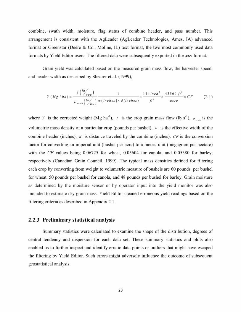
Grain yield was calculated based on the measured grain mass flow, the harvester speed,

and header width as described by Shearer et al. (1999),

2 2

2

 1 1 4 4   4 3 5 6 0  

 ( / )      ( ) 

g ra in

lbfin c h fts e c

Y M g h a C Flb w in c h e s d in c h e s ft a c r e

b u

(2.1)

where Y is the corrected weight (Mg ha-1

), f is the crop grain mass flow (lb s-1

), g r a in

is the

volumetric mass density of a particular crop (pounds per bushel), w is the effective width of the

combine header (inches), d is distance traveled by the combine (inches). C F is the conversion

factor for converting an imperial unit (bushel per acre) to a metric unit (megagram per hectare)

with the CF values being 0.06725 for wheat, 0.05604 for canola, and 0.05380 for barley,

respectively (Canadian Grain Council, 1999). The typical mass densities defined for filtering

each crop by converting from weight to volumetric measure of bushels are 60 pounds per bushel

for wheat, 50 pounds per bushel for canola, and 48 pounds per bushel for barley. Grain moisture

as determined by the moisture sensor or by operator input into the yield monitor was also

included to estimate dry grain mass. Yield Editor cleaned erroneous yield readings based on the

filtering criteria as described in Appendix 2.1.

2.2.3 Preliminary statistical analysis

Summary statistics were calculated to examine the shape of the distribution, degrees of

central tendency and dispersion for each data set. These summary statistics and plots also

enabled us to further inspect and identify erratic data points or outliers that might have escaped

the filtering by Yield Editor. Such errors might adversely influence the outcome of subsequent

geostatistical analysis.

24

The R statistical software package version 2.15.3 (R Development Core Team, 2013) was

used to draw histograms of raw and filtered yield data and quantile-quantile plots. The usual

summary statistics including minimum, maximum, mean, standard deviation, coefficient of

variation, skewness, and kurtosis for raw and filtered data were also calculated. The normality of

each cleaned yield data was tested with the Kolmogorov-Smirnov statistic as implemented in

SAS PROC UNIVARIATE (SAS Institute Inc, 2014). However, the high sensitivity of the

Kolmogorov-Smirnov statistic to large sample sizes as in our data sets made it of little practical

value. Thus, the significance of the normality test was also assessed by examining the observed

skewness and kurtosis of the data as well as inspecting quantile-quantile (Q-Q) plots. The overall

assessment suggested that no data transformation was required prior to geostatistical analysis.

2.2.4 Geostatistical analysis

For each crop year, the cleaned data were standardized as,

' i

i

y

y yy

s

(2.2)

where '

iy is the standardized yield value at the ith location in the field,

iy is the observed yield

value at the same location, y is the average yield value for the crop year, and y

s is the standard

deviation of the yield values. This was done to remove the scaling effect for yield data sets from

different crop years, thereby allowing for the comparison of spatial yield patterns across multiple

years and crops from the same field.

Spatial patterns in the yield data were investigated through plots of semivariograms (or

sometimes called semivariances) against corresponding geographic distances between data

points. Since individual yield readings were separated by varying geographical distances, a

semivariogram or semivariance value for a given distance or a lag interval (h) was calculated as

half the mean of squared differences between all possible pairs of yield readings found within

this lag interval (Cressie, 1993; Isaaks and Srivastava, 1989; Journel and Huijbregts, 1978;

Webster and Oliver, 2007):

25

( )2

1

1( )

2 ( )

N h

i ih z u z u h

N h (2.3)

where ( )h is the semivariance estimator, ( )N h is the number of pairs of yield points separated

by lag interval h , i

u denotes the spatial coordinates at locations i , ( )i

z u and ( )i

z u h denote

ith pair of yield observations separated by h . It is evident from Equation (2.3) that ( )h

increases with distance until a plateau is reached. The distance at this plateau is known as the

range (Oliver, 2013). In the absence of spatial correlation (i.e., a random distribution of yield

readings anywhere over the entire field), the semivariance values would not be expected to

change with the increase in h , and they would be constant over all distances. In the presence of

spatial autocorrelation, however, the semivariogram values would be small at short distances,

and increase rapidly at intermediate distances, and reach to an asymptote at the range beyond

which there is little change in the semivariance.

Semivariogram values were plotted against the corresponding distances for each crop

year. These variogram plots were fitted by three commonly used spatial covariance models,

exponential, Gaussian and spherical, using the weighted least-squares method (Cressie, 1993).

The GSTAT/R package (Pebesma, 2004) was used for model fitting. As shown in Figure 2.1,

each covariance model contains three unknown parameters: the nugget (0

c ) measuring random

variation among data points at zero or close proximity, the structural variance or partial sill (1

c )

measuring part of the total variation or sill (0 1

c c ) due to spatial pattern and a is the range

beyond which there is little spatial correlation. Thus, the nugget/sill ratio would be a convenient

measure of the level of spatial dependence, with the spatial dependence being classified as

strong, medium and weak if the ratio is <25%, 25-75% and >75%, respectively (Cambardella et

al., 1994).

The three unknown model parameters were estimated during the model fitting and they

entered the three covariance models somewhat differently. The spherical model exhibits linear

behaviour near the origin and reaches the sill quicker than any other model and its functional

form is described as:

26

3

0 1

0 1

3 1      , 0  

2 2

  , 

h hc c h a

h a a

c c h a

(2.4)

The Gaussian model shows a parabolic behaviour near the origin and reaches the sill

asymptotically. It is a useful model if data exhibit a strong spatial autocorrelation at the shortest

lag distance. It can be expressed as:

2

0 1( ) 1 , 0

h

ah c c e h

(2.5)

The exponential model is similar to the spherical model with linear behaviour being near the

origin but it reaches the sill asymptotically as lag distance becomes large. It assumes that the

correlation never reaches exactly zero irrespective of how far apart the points are. It is expressed

as:

0 1        1   , 0

h

ah c c e h

(2.6)

The exponential and Gaussian models approach the sill asymptotically, with 3a and

3 a being the practical ranges for these two models, respectively. The practical range is the

distance at which the semivariance, h , reaches 95% of the sill (Webster, 1985; Webster and

Oliver, 2007).

27

2.2.5 R programs for geostatistical analysis

A full description of R code is given in Appendix 2.2 with detailed comments on the use

of GSTAT and associated R packages for data preparation, variogram calculation and model

fitting. Here are some highlights of those R functionalities.

2.2.5.1 Data preparation

For the geostatistical analysis, each data set consisted of three columns: longitude and

latitude (spatial component), and yield (attribute component). This data format was required for

the implementation of variogram analysis with GSTAT/R. After each data was loaded into the

GSTAT/R environment, a spatial object was created using the coordinates() function. We

transformed from spherical coordinates (longitude and latitude) to universal transverse mercator

(UTM) i.e. easting and northing in meters by projecting onto a two-dimensional planar surface

using spTransform() function. The use of the UTM projection enabled more accurate estimation

of distances between data points. Under the UTM system, the Earth is divided into sixty (60)

zones, each spanning 6° of longitude. The new projected coordinates were all within zone 12

(114 oW to 108

oW) where the farm field is located on Earth. The origin of zone 12 in the

eastings direction is a point 500,000 metres west of the central meridian (111 oW) of the zone

whereas the origin in the northings direction is the equator. The estimated distance between a

pair of yield readings in the field was measured in meters.

2.2.5.2 Calculating empirical variogram

The empirical variogram was calculated using the variogram() function for the response

variable yield. In this calculation, the observed yield [ ( )z u ] is modeled as the sum of a spatial

trend ( )u and a random residual ( )u :

( ) ( ) ( )z u u u . (2.7)

This essentially follows a random field (RF) theory in which the total spatial variability can be

partitioned into a large-scale spatial trend (e.g., directional or anisotropic effects) and small-scale

variation (Cressie, 1993, p. 46-60). The variogram() function consists of more than 2 arguments

28

to accommodate the variogram calculations under different scenarios. For our study, we used the

non-default values for the following arguments. The cutoff argument was set to be 300 m, a

maximum distance between pairs of yield readings within which the variograms were computed.

In other words, no variogram value was computed for those yield readings separated by more

than 300 m. The choice of this distance threshold (300 m) was based on our preliminary analysis

that there would be little spatial dependency between yield points with a distance of >300 m.

This threshold was only about half the default value given in GSTAT/R, which is equal to the

length of the diagonal of the rectangle spanning the data being divided by three (

2 21603 795 / 3 = 1,789/3 ~600 m). The width = 5 argument was given to instruct GSTAT/R

to use the lag distance interval of 5 m. The choice of 5 m for a lag distance was based again on

our preliminary analysis which showed a less precise variogram plot for >5 m or an erratic

variogram plot for <5 m. The isotropic empirical variogram was computed because our

preliminary analysis showed that four directional values (alpha = 0°, 45°, 90°, and 135°) had

little influence on empirical variogram values. Finally, the cressie argument was set to a logical

value of TRUE in order to obtain a robust empirical variogram with estimators that would

alleviate the effect of spatial outliers as proposed by (Cressie and Hawkins, 1980).

2.2.5.3 Fitting theoretical models to empirical variograms

For model fitting, we developed a method to obtain appropriate initial values of range,

partial sill and nugget which are critical in ensuring the convergence of fitting nonlinear models

such as the three spatial covariance models used in this study. The method worked as follows.

All pairs of empirical semivariograms for a given dataset were sorted according to their

geographic distances in an ascending order. The first step was to estimate the sill as an average

of the top-ranking 20% of semivariogram values (i.e., all the semiovariograms between the 81st

and 100th

percentiles). The initial value of the range was estimated as the distance from the 81

percentile of the sorted semivariograms to the origin. Once the range was determined, the 5% of

the semivariograms with the shortest distances within the range were averaged to provide the

initial value of nugget. The difference between sill and nuggest estimates was used as the initial

value of the partial sill. Exponential, Gaussian, and spherical covariance models were fitted to

the variogram plot for the data set in each crop year using vgm() and fit.variogram() functions.

29

The vgm() function generated a variogram model using initial values of partial sill, range, and

nugget as just described. The covariance models were fitted to the variogram plot using the

fit.variogram() function. Even though there are several methods of model fitting as shown in

Appendix 2.3, this study employed a default method, fit.method = 7, known as the weighted

least-squares (WLS) method (Cressie, 1993). The WLS fitting method is the popular choice

among variogram model estimation methods because of its robustness and its freedom from any

distributional requirements (Cressie, 1985).

2.2.6 Goodness-of-fit and Cross validation

Each fitted model was assessed for its goodness-of-fit in several ways. First, the weighted

sum of squares errors statistic (SSErr) was computed using the attrib() function from the

GSTAT/R package (Pebesma, 2004). The SSErr was given by,

2

2

1

ˆ    

b

i

i i

i i

NS S E r r h h

h

(2.8)

where 𝛾(ℎ𝑖) is the model semivariogram for the ith distance class (bin) with the lag distance of

hi; 𝛾(ℎ𝑖) is the empirical semivariogram for the same distance bin; b is the number of lag bins;

iN and

ih define the weighting factor

2

i

i

N

h which is the ratio of the number of point pairs and

squared separation distance for the ith distance bin.

Second, a preliminary analysis was carried out with a subset of the data (i.e., the first

1200 observations from the data set) using SAS PROC MIXED (SAS Institute Inc, 2014) with

the TYPE=SPH, GAU and EXP options for spherical, Gaussian and exponential models being

specified in the REPEATED statement, respectively. The MIXED analysis of the full data set

was not feasible because the size of covariance matrix generated was too large to be handled by

the mixed-model analysis. This preliminary analysis, while based only on a subset of data, was

carried out with intent to confirm the usefulness of the SSErr statistic as a measure of goodness-

of-fit for model comparison. The model selection criteria included Akaike Information Criterion

(AIC) and Bayesian Information Criterion (BIC) as generated by SAS PROC MIXED (Appendix

2.5).

30

The third way to assess the adequacy of a variogram model was to inspect the ratio of the

partial sill (psill) to the sill (psill/sill). A variogram model with the least SSErr and a psill/sill

ratio close to 1.0 would be considered the best-fitting variogram model. The closeness of

psill/sill ratio to 1.0 signifies that the nugget effect is negligible, suggesting a very strong spatial

structure (Raper et al., 2005).

Finally, each fitted model was further validated through cross validation. We employed

the krige.cv() function with the nfold = 5 argument as implemented in GSTAT/R (Pebesma,

2004) to do the five-fold cross validation. For the five-fold cross validation, each data was

randomly partitioned in five parts, each of which was used once as the validation data set for

testing the model (exponential, Gaussian or spherical), and the remaining four parts were used as

the training data set. For validation, predictions were made using the local kriging (Cressie,

1993) based on a maximum neighborhood size of 20 observations as specified using the nmax =

20 argument in the validation data set. This cross validation procedure was repeated for each of

the 5 parts for the yield data in each crop year using the krige.cv() function of GSTAT/R. Two

diagnostic statistics are returned: (i) Pearson’s correlation between observed and predicted values

and (ii) the root of mean square error (RMSE). The RMSE is given by,

2

1ˆ 

R M S E =

n

i iiz u z u

n

(2.9)

where n is number of validation points, ( )i

z u is the observed yield and ˆ ( )i

z u is the predicted

value.

31

2.3 Results

All filtering criteria except for flow delay were applied to the yield monitor data set in

each of the four crop years (Table 2.2). The overall percentages of erroneous yield values

removed by the filtering criteria ranged from 3.78% for canola in 2009 to 5.99% for wheat in

2010. Different filtering criteria as described in Appendix 2.1 were not mutually exclusive. A

large proportion of the errors removed was attributed to the minimum velocity filter.

The cleaned yield readings for each of the four crop years were mapped (Figure 2.3).

These yield maps showed that the shape of the field was somewhat a tilted rectangle with the

northeast corner being missing. The tilting is due to the use of UTM projection system. In

addition, there was an extended strip area on the west side of the field with no yield readings in

year 2008. The estimates of data densities varied among the four crop years, from 711.9 (canola

2009) to 1110.7 (wheat 2008) yield readings per hectare (Table 2.3). These estimates were based

on the averages of swath width and interval for yield reading recorded for each crop year. The

estimated swath widths were all shorter than 10 m, the actual swath width of the combine,

ranging from 7.3 m in 2009 to 9.0 m in 2010 and 2011. The estimated recording frequencies

were also different among the four years, ranging from 1.1 m (2008) to 1.9 m (2009) per yield

reading. The product of swath width and recording interval gave an estimate of the area covered

for one yield reading, thereby varying among the four years accordingly.

The histograms and Q-Q plots of the raw vs. cleaned yield readings are presented in

Figures 2.4-2.7 for four crop years. The noisiness of the raw data sets was quite evident from a

highly skewed distribution with a higher coefficient of variation (CV = 14.5 to 20.5%) and a

huge range 0.29 Mg ha-1

(~4 standard deviation less than mean) to 26.65 Mg ha-1

(~14 standard

deviation higher than mean). The range far exceeded the biological yield limits (Table 2.4). The

cleaned data sets improved yield distributions to approximately normal as shown in the

histograms and Q-Q plots though the Kolmogorov-Smirnov test for normality. This result is

hardly surprising given that the sample size is very large in all four data sets.

Variogram plots for all four datasets are presented in Appendix 2.7 with each figure

displaying variogram plots in four directions. Visual inspection of these plots showed no

32

difference in spatial dependence with change in direction. Given these observations, isotropic

variograms were provided (Figures 2.8 – 2.11).

The exponential function had the least values of SSErr and the psill/sill ratios closest to

1.0 for the four crop years (Table 2.5). These results were consistent with the preliminary

analysis of the subsets of the data sets using SAS PROC MIXED with the exponential function

having the smallest AIC and BIC values (Appendix 2.5). Therefore, an exponential covariance

model with appropriate model parameters is more adequate to describe the empirical variograms

of yield for the four crop years.

Table 2.6 presents the root mean square error (RMSE) and correlation coefficient

between the observed and predicted yields as diagnostic statistics from cross validation. The

results revealed that the spherical and exponential models gave similar prediction accuracy.

However, with joint consideration of the results given in Table 2.5, the exponential model would

be considered the most appropriate model for describing spatial variability in this farm field.

The estimated ranges based on an exponential model from the variogram plots varied

from 39.6 m for wheat in 2008 to 99.6 m for canola in 2009 (Table 2.7). The estimates of nugget

varied from 0.31 in 2008 to 0.51 in 2010 while the estimates of total semivariance or sill were

relatively consistent across crop years with a narrow range of 0.84 (2010) to 0.88 (2009).

33

2.4 Discussion

The frequency distributions of each filtered data were approximately normal, indicating

that the removal of extreme values or outliers was effective. The similar means observed in raw

and cleaned data sets suggests that the erroneous data being removed from both sides of the

mean were approximately equal. The proportions of erroneous values being removed varied from

3.78% to 5.99%, which are much smaller than 10-50% as reported in the literature (Blackmore

and Moore, 1999; Simbahan et al., 2004; Thylen et al., 2000). This is likely due to the fact that

the set of raw datasets are fairly cleaned already, judging from the relatively low CV (14.5 to

20.5%). Indeed, we confirmed no need for calibrating flow delay after detailed examination of

the raw data sets with different levels of flow delay. The cleaned yields had low CV values

(between 11.2 and 17.9%). Our CV values for the cleaned data sets are lower than the CV values

(26 and 58%) reported by Guedes Filho et al. (2010a) but similar to those (13 and 29.7%)

reported by Faechner and Benard (2006) who evaluated spatial variability of yields for crops

grown on and off reclaimed industrial sites in Alberta.

In all study years (2008 to 2011), the crop yields had a spatial structure described by an

exponential variogram model. This is similar to results reported by O'Halloran et al. (2004) for

examining spatial variability of barley and corn yields. Guedes Filho et al. (2010b) reported a

spherical variogram model for characterizing spatial variability of different crops grown in a

rotation system under no-tillage. While the report of Guedes Filho et al. (2010b) appears contrary

to our finding, a spherical model would have been equally adequate, judging from our prediction

accuracy results (Table 2.6) and model parameter estimates (Appendix 2.6)

The variation in the nugget/sill ratios across crop years signifies the magnitude of local-

scale stochastic variability for each year. The ratios also indicated a moderate degree of spatial

dependency according to the classification scheme of Cambardella et al. (1994). Our ratios were

similar to those reported by Guedes Filho et al. (2010b). Our range estimates varied from 39.6 m

for wheat-2008 to 99.6 m for canola-2009. Barley-2011 had a practical range of 59.4 m which

was within the values 57 to 85 m as reported by O'Halloran et al. (2004). The reason for a greater

range of spatial correlation for canola is unknown, but may be attributed to management factors,

weather effects or crop rotation.

34

The estimates of model parameters with an exponential covariance model (Table 2.7)

varied from one crop year to another, likely reflecting the fact that different years underwent

different environmental conditions (precipitation, temperature), management practices, and

different crops. Since the yield data were standardized, the nugget and sill estimates would be the

estimated percentages of total variation. The sill should represent the total variance and thus an

unbiased estimate of the sill would be close to 100% (the variance of the standardized variate

would be one). However, while similar estimates of the sill were found across the four years

from 84% (2010) to 88% (2009) of the total variance, they were all obviously underestimated.

This underestimation of the sill indicates that a cutoff of 300 m used as the practical range is

likely shorter than the ‘true’ range. The nugget estimates varied from 31% (2008) to 51% (2010)

of the total variation, indicating the year-to-year variation in measurement error and/or variation

at distances less than the sampling interval. The range estimates varied from 39.6 m in 2008 to

99.6 m in 2009. This variation corresponded well to the difference in data densities between the

years from 9.0 m2 per observation or 1110.7 observations per hectare in 2008 to 14.0 m

2 per

observation in 2009 or 711.9 observations per hectare (Table 2.3).

The results from this study have several practical implications. First, while an exponential

covariance model was identified as the best fitted model across the four years, the estimates of

the model parameters (particularly the estimated ranges in the study) varied from year to year,

suggesting that spatial patterns may still be quite different across the years. There seems to be a

close association between the estimated ranges (Table 2.7) and the amount of growing-season

precipitation (Table 2.1): the year with a largest estimated range (2009) had the driest growing

season while the year with a smallest estimated range (2008) had the wettest growing season.

Such association needs to be confirmed in future studies in which in-field weather stations are

required to record in-situ temperatures and precipitations rather than the weather data from a

neighboring region. As water is typically a limiting factor to crop production in Alberta and

western Canada, yield variation may vary widely from a dry year to a wet year. Thus, when the

estimates of model parameters varied greatly among successive cropping years, using only one

year of yield data may not provide a reliable estimator to make informed decisions. Second,

patterns of spatial variability along with different estimates of the model parameters for crops

grown in the four years may be partly reflective of differences in crop characteristics, growth

patterns and needs, and differential responses to crop inputs and environmental conditions. For

35

example, the same wheat variety (AC Harvest) was grown in years 2008 and 2010, but there

were differences in crop inputs (seeding rate, fertilizer formula and rate) and weather conditions

between the two years (Table 2.1). It appears that the crop inputs and weather conditions in 2010

were resulted in more fine-scaled, localized (≤ 5 m) random fluctuations among yields (nugget =

0.51) than those in 2008 (nugget = 0.31) while estimates of the total variation were similar in

both years (sill = 0.86 in 2008 and 0.84 in 2010). These model-based estimates of nugget were

further confirmed by the averages of all empirical semivariograms for yield pairs separated by 5

meters (0.39 in 2008 vs. 0.53 in 2010). Thus, the crop inputs and growing conditions may impact

spatial pattern and extent. Future studies may be designed to investigate the influences of

individual factors, singly or collectively, on the spatial pattern and extent. Third, the amount of

random noise (nugget = 31% to 51% of the total variation) from our study is quite large even

with relatively high data densities (1 – 2 m per yield reading; cf. Table 2.3). Our averaged grids

of yield recording (Table 2.3) were finer than those of Faechner and Benard (2006) who

recommended that a minimum of 72 to 120 data points over a 100 m × 100 m area on a farm

field would be required for a valid statistical comparison between yields recorded by GPS yield

monitoring technology from on and off oil-well sites in the field. Their recommendation was

based on much smaller estimates of nugget (≤ 5%). Their comparison attempted to establish a

yield-based reclamation criterion to substantiate the current vegatation-based criterion that crops

growing on the reclaimed (on-site) area meet or exceed 80% of the density and height of

vegetation in comparison to a normal, off-site area in the field (Alberta Government, 2013).

Thus, in the cultivated farm lands with the large nugget effect within a small scale as observed in

our study, a more dense sampling of yields (~700 to 1110 yield readings per 100 m × 100 m

area) would be needed for a valid comparison between on- and off-well yields.

This study focused on the analysis of one type of georeferenced data (yield monitor data).

With the advent of many geomatics-based technologies, other types of georeferenced data

(imagery data and sensor-based EC data) characterizing yield-limiting factors will become

increasingly available. Future studies will integrate yield data (e.g., in this study) and those new

data for identifying key factors influencing the crop yield. It is also evident from this study that

the yield data sets in four crop years have different data densities (Table 2.3) , indicating yield

readings are not aligned across the years. This lack of alignment of yield readings across four

years makes it difficult to pool the data together for a combined analysis. In order to assess the

36

stability pattern of yields over the years, one suggestion is to generate a common grid through

which spatial interpolation can be used to predict yields at the vertices of the common grid. This

will be described in detail in Chapter Three.

2.5 Summary and Conclusion

This study evaluates the spatial patterns of yields using geostatistical methods for three

crops grown between 2008 and 2011 from the same production field. Classical statistical

techniques such as regression and ANOVA are inappropriate for quantifying the spatial

variability of yield monitor data from field-scale data where the spatial correlation exist among

densely subsampled yield readings. The spatial pattern for the data set in each crop year was

assessed and detected by geostatistical tools including variogram plotting and modeling. Prior to

such an assessment and detection, data quality control measures were taken by filtering

erroneous values that might be attributed to sampling error and errors of combine harvester.

The findings of this study reveal that spatial pattern of crop yields could be best described

by an exponential covariance model in each crop year but the estimates of model parameters

were different over the years (Table 2.7). These findings have several practical implications for

the use of yield monitor data for precision agriculture practices such as delineation of

management or production zones for site specific management.

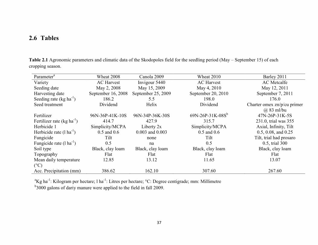
37

2.6 Tables

Table 2.1 Agronomic parameters and climatic data of the Skodopoles field for the seedling period (May – September 15) of each

cropping season.

Parametera Wheat 2008 Canola 2009 Wheat 2010 Barley 2011

Variety AC Harvest Invigour 5440 AC Harvest AC Metcalfe

Seeding date May 2, 2008 May 15, 2009 May 4, 2010 May 12, 2011

Harvesting date September 16, 2008 September 25, 2009 September 20, 2010 September 7, 2011

Seeding rate (kg ha-1

) 186.2 5.5 198.0 176.0

Seed treatment Dividend Helix Dividend Charter omex zn/p/cu primer

@ 83 ml/bu

Fertilizer 96N-36P-41K-10S 96N-34P-36K-30S 69N-26P-31K-08Sb 47N-26P-31K-5S

Fertilizer rate (kg ha-1

) 414.7 427.9 315.7 231.0, trial was 355

Herbicide 1 Simplicity/MCPA Liberty 2x Simplicity/MCPA Axial, Infinity, Tilt

Herbicide rate (l ha-1

) 0.5 and 0.6 0.003 and 0.003 0.5 and 0.6 0.5, 0.08, and 0.25

Fungicide Tilt none Tilt Tilt, trial had prosaro

Fungicide rate (l ha-1

) 0.5 na 0.5 0.5, trial 300

Soil type Black, clay loam Black, clay loam Black, clay loam Black, clay loam

Topography Flat Flat Flat Flat

Mean daily temperature

(°C)

12.85 13.12 11.65 13.07

Acc. Precipitation (mm) 386.62 162.10 307.60 267.60

aKg ha

-1: Kilogram per hectare; l ha

-1: Litres per hectare; °C: Degree centigrade; mm: Millimetre

b3000 galons of dariy manure were applied to the field in fall 2009.

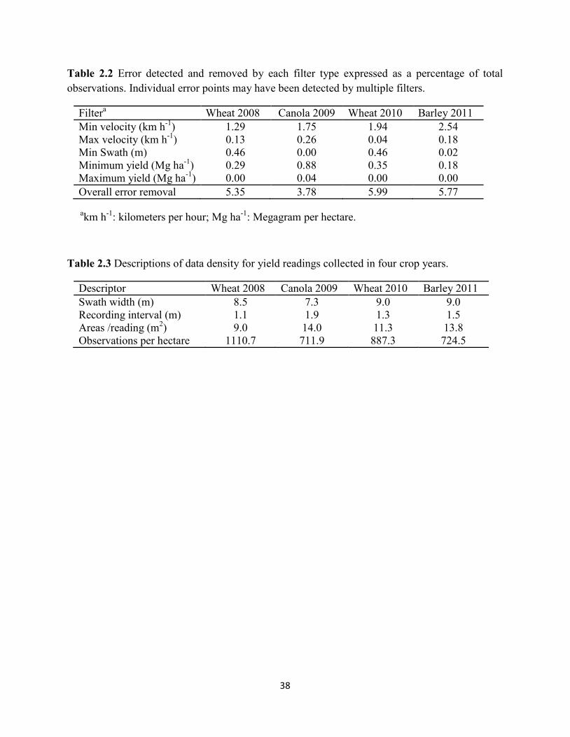
38

Table 2.2 Error detected and removed by each filter type expressed as a percentage of total

observations. Individual error points may have been detected by multiple filters.

Filtera Wheat 2008 Canola 2009 Wheat 2010 Barley 2011

Min velocity (km h-1

) 1.29 1.75 1.94 2.54

Max velocity (km h-1

) 0.13 0.26 0.04 0.18

Min Swath (m) 0.46 0.00 0.46 0.02

Minimum yield (Mg ha-1

) 0.29 0.88 0.35 0.18

Maximum yield (Mg ha-1

) 0.00 0.04 0.00 0.00

Overall error removal 5.35 3.78 5.99 5.77

akm h

-1: kilometers per hour; Mg ha

-1: Megagram per hectare.

Table 2.3 Descriptions of data density for yield readings collected in four crop years.

Descriptor Wheat 2008 Canola 2009 Wheat 2010 Barley 2011

Swath width (m) 8.5 7.3 9.0 9.0

Recording interval (m) 1.1 1.9 1.3 1.5

Areas /reading (m2) 9.0 14.0 11.3 13.8

Observations per hectare 1110.7 711.9 887.3 724.5

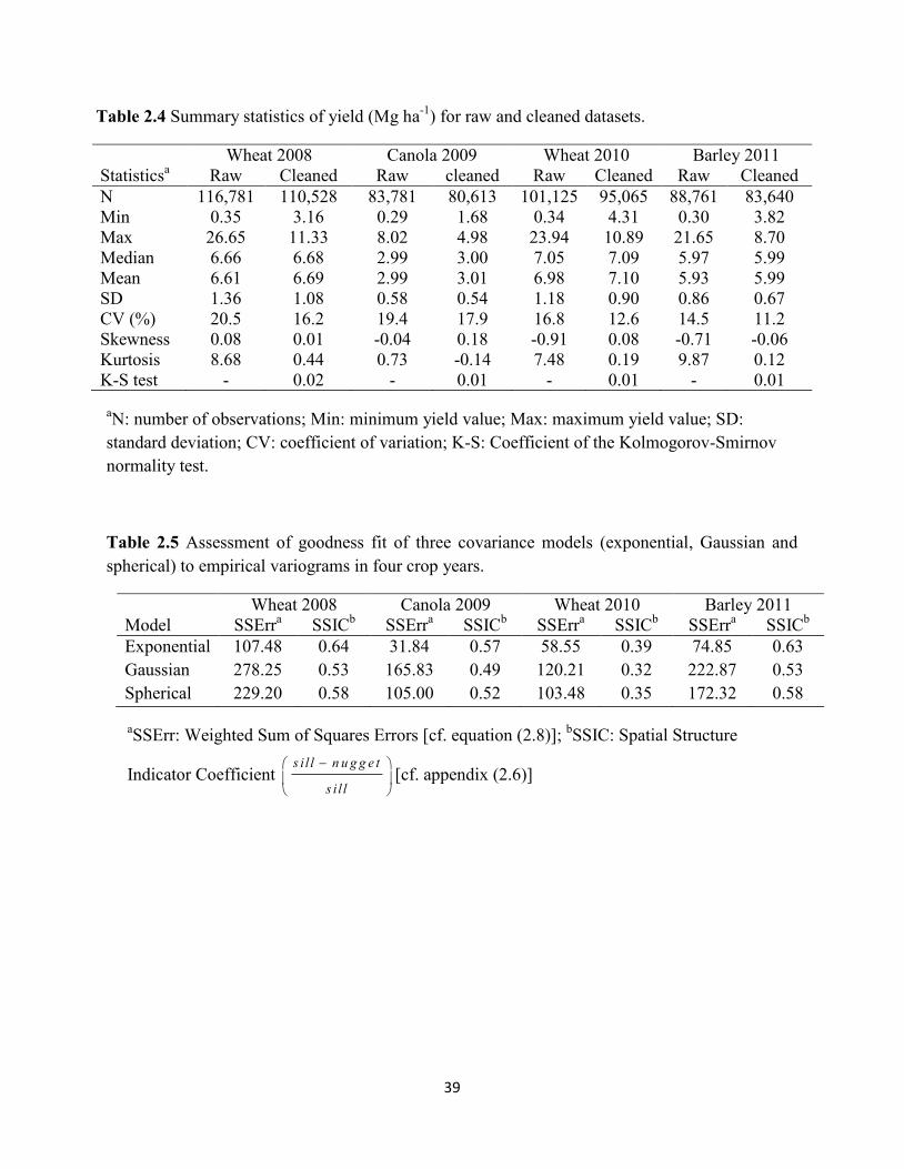
39

Table 2.4 Summary statistics of yield (Mg ha-1

) for raw and cleaned datasets.

Wheat 2008 Canola 2009 Wheat 2010 Barley 2011

Statisticsa Raw Cleaned Raw cleaned Raw Cleaned Raw Cleaned

N 116,781 110,528 83,781 80,613 101,125 95,065 88,761 83,640

Min 0.35 3.16 0.29 1.68 0.34 4.31 0.30 3.82

Max 26.65 11.33 8.02 4.98 23.94 10.89 21.65 8.70

Median 6.66 6.68 2.99 3.00 7.05 7.09 5.97 5.99

Mean 6.61 6.69 2.99 3.01 6.98 7.10 5.93 5.99

SD 1.36 1.08 0.58 0.54 1.18 0.90 0.86 0.67

CV (%) 20.5 16.2 19.4 17.9 16.8 12.6 14.5 11.2

Skewness 0.08 0.01 -0.04 0.18 -0.91 0.08 -0.71 -0.06

Kurtosis 8.68 0.44 0.73 -0.14 7.48 0.19 9.87 0.12

K-S test - 0.02 - 0.01 - 0.01 - 0.01

aN: number of observations; Min: minimum yield value; Max: maximum yield value; SD:

standard deviation; CV: coefficient of variation; K-S: Coefficient of the Kolmogorov-Smirnov

normality test.

Table 2.5 Assessment of goodness fit of three covariance models (exponential, Gaussian and

spherical) to empirical variograms in four crop years.

Wheat 2008 Canola 2009 Wheat 2010 Barley 2011

Model SSErra SSIC

b SSErr

a SSIC

b SSErr

a SSIC

b SSErr

a SSIC

b

Exponential 107.48 0.64 31.84 0.57 58.55 0.39 74.85 0.63

Gaussian 278.25 0.53 165.83 0.49 120.21 0.32 222.87 0.53

Spherical 229.20 0.58 105.00 0.52 103.48 0.35 172.32 0.58

aSSErr: Weighted Sum of Squares Errors [cf. equation (2.8)];

bSSIC: Spatial Structure

Indicator Coefficient s i l l n u g g e t

s i l l

[cf. appendix (2.6)]

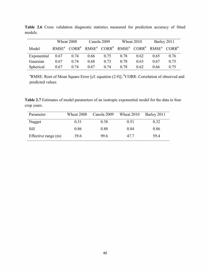
40

Table 2.6 Cross validation diagnostic statistics measured for prediction accuracy of fitted

models.

Wheat 2008 Canola 2009 Wheat 2010 Barley 2011

Model RMSEa CORR

b RMSE

a CORR

b RMSE

a CORR

b RMSE

a CORR

b

Exponential 0.67 0.74 0.66 0.75 0.78 0.62 0.65 0.76

Gaussian 0.67 0.74 0.68 0.73 0.78 0.63 0.67 0.75

Spherical 0.67 0.74 0.67 0.74 0.78 0.62 0.66 0.75

aRMSE: Root of Mean Square Error [cf. equation (2.9)];

bCORR: Correlation of observed and

predicted values

Table 2.7 Estimates of model parameters of an isotropic exponential model for the data in four

crop years.

Parameter Wheat 2008 Canola 2009 Wheat 2010 Barley 2011

Nugget 0.31 0.38 0.51 0.32

Sill 0.86 0.88 0.84 0.86

Effective range (m) 39.6 99.6 47.7 59.4

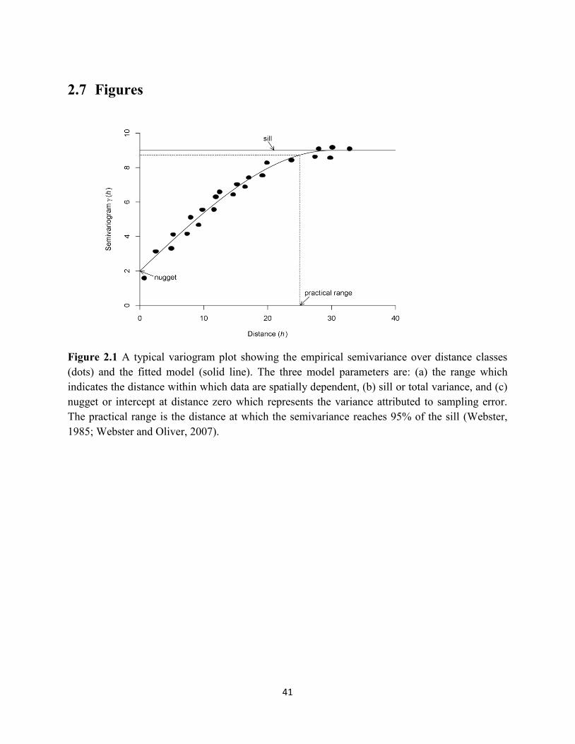
41

2.7 Figures

Figure 2.1 A typical variogram plot showing the empirical semivariance over distance classes

(dots) and the fitted model (solid line). The three model parameters are: (a) the range which

indicates the distance within which data are spatially dependent, (b) sill or total variance, and (c)

nugget or intercept at distance zero which represents the variance attributed to sampling error.

The practical range is the distance at which the semivariance reaches 95% of the sill (Webster,

1985; Webster and Oliver, 2007).

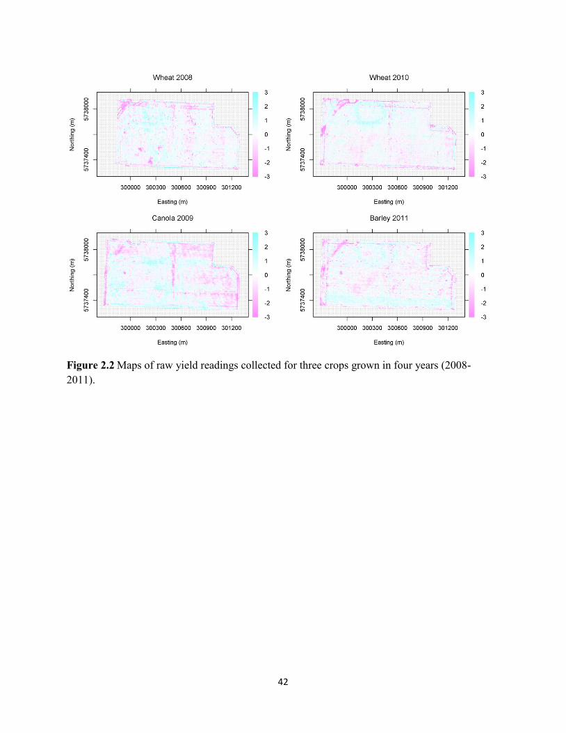
42

Figure 2.2 Maps of raw yield readings collected for three crops grown in four years (2008-

2011).

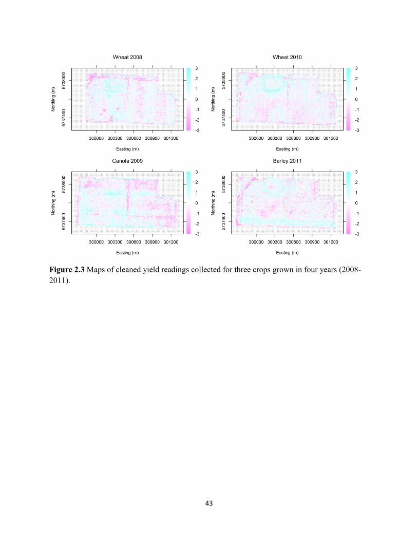
43

Figure 2.3 Maps of cleaned yield readings collected for three crops grown in four years (2008-

2011).

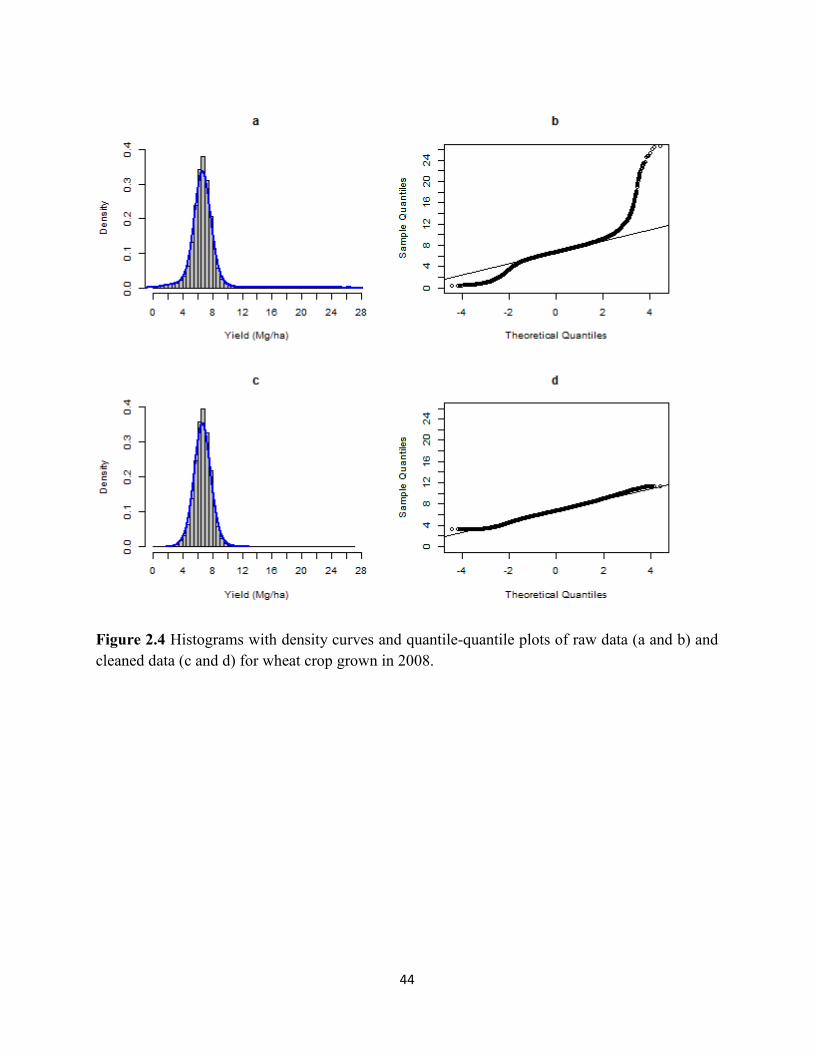
44

Figure 2.4 Histograms with density curves and quantile-quantile plots of raw data (a and b) and

cleaned data (c and d) for wheat crop grown in 2008.

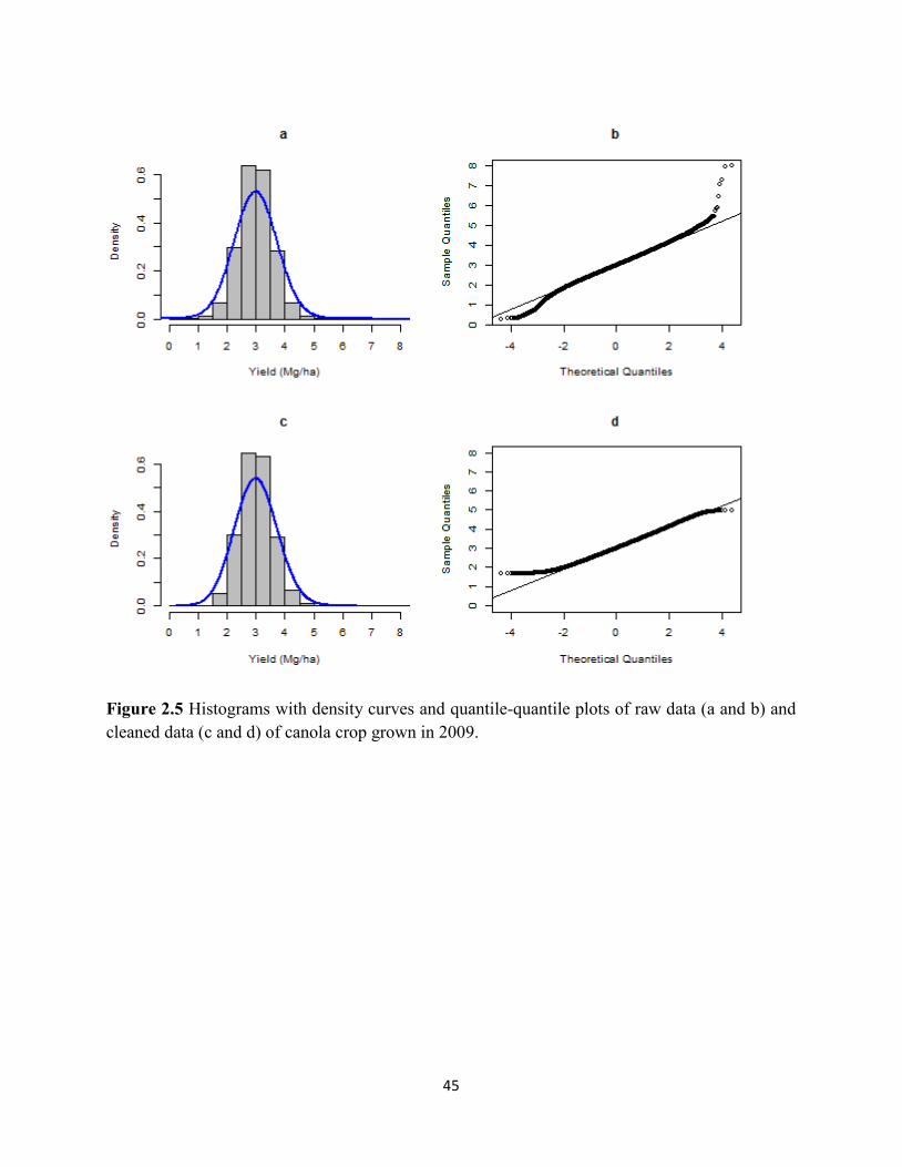
45

Figure 2.5 Histograms with density curves and quantile-quantile plots of raw data (a and b) and

cleaned data (c and d) of canola crop grown in 2009.

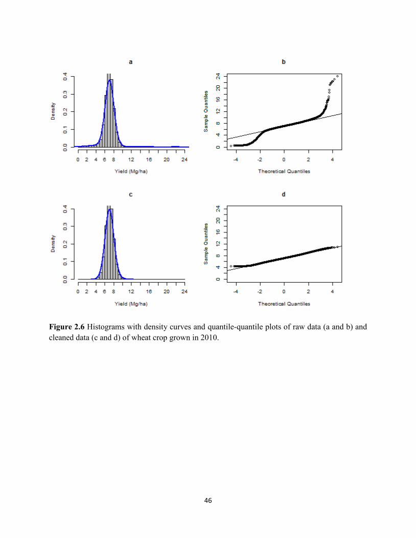
46

Figure 2.6 Histograms with density curves and quantile-quantile plots of raw data (a and b) and

cleaned data (c and d) of wheat crop grown in 2010.

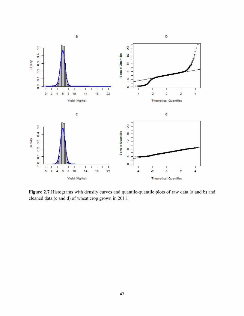
47

Figure 2.7 Histograms with density curves and quantile-quantile plots of raw data (a and b) and

cleaned data (c and d) of wheat crop grown in 2011.

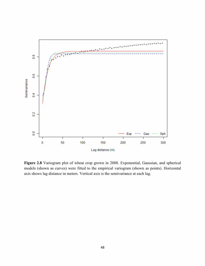
48

Figure 2.8 Variogram plot of wheat crop grown in 2008. Exponential, Gaussian, and spherical

models (shown as curves) were fitted to the empirical variogram (shown as points). Horizontal

axis shows lag distance in meters. Vertical axis is the semivariance at each lag.

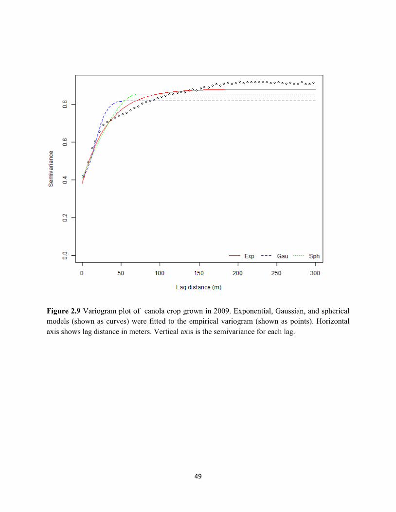
49

Figure 2.9 Variogram plot of canola crop grown in 2009. Exponential, Gaussian, and spherical

models (shown as curves) were fitted to the empirical variogram (shown as points). Horizontal

axis shows lag distance in meters. Vertical axis is the semivariance for each lag.

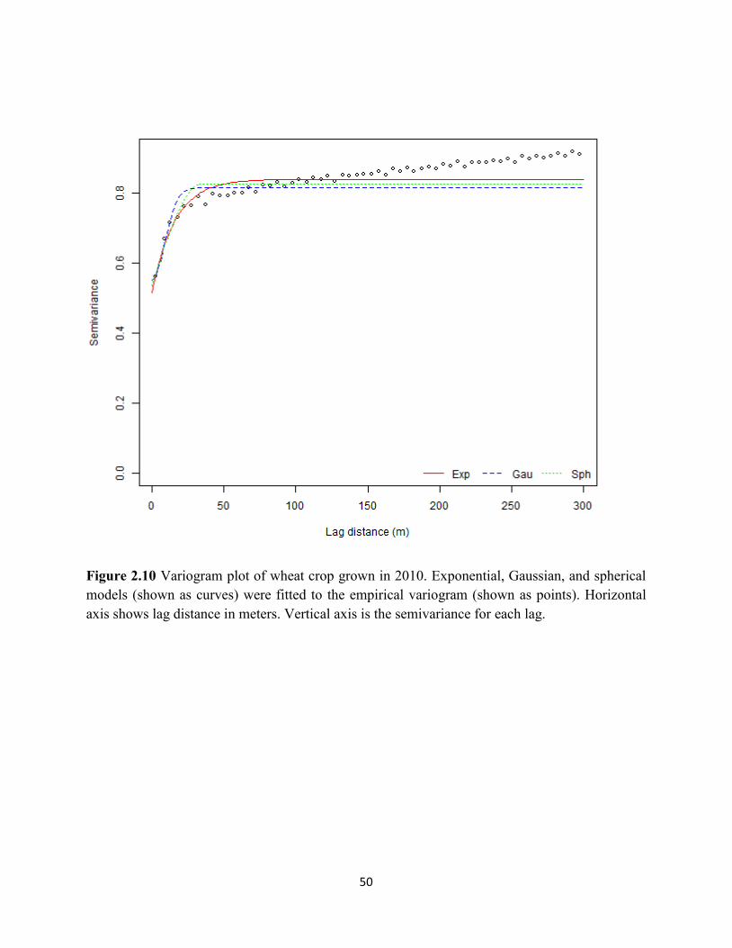
50

Figure 2.10 Variogram plot of wheat crop grown in 2010. Exponential, Gaussian, and spherical

models (shown as curves) were fitted to the empirical variogram (shown as points). Horizontal

axis shows lag distance in meters. Vertical axis is the semivariance for each lag.

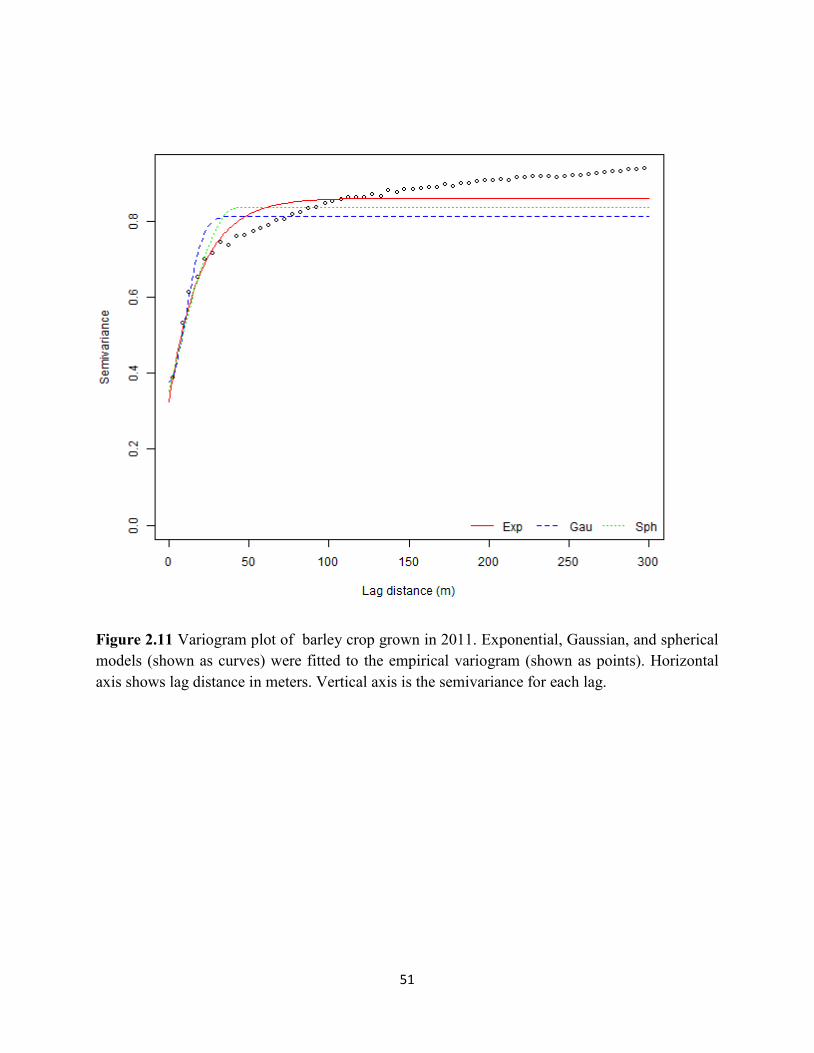
51

Figure 2.11 Variogram plot of barley crop grown in 2011. Exponential, Gaussian, and spherical

models (shown as curves) were fitted to the empirical variogram (shown as points). Horizontal

axis shows lag distance in meters. Vertical axis is the semivariance for each lag.

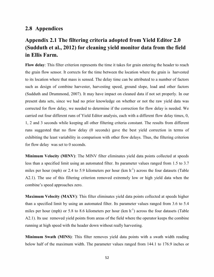
52

2.8 Appendices

Appendix 2.1 The filtering criteria adopted from Yield Editor 2.0

(Sudduth et al., 2012) for cleaning yield monitor data from the field

in Ellis Farm.

Flow delay: This filter criterion represents the time it takes for grain entering the header to reach

the grain flow sensor. It corrects for the time between the location where the grain is harvested

to its location where that mass is sensed. The delay time can be attributed to a number of factors

such as design of combine harvester, harvesting speed, ground slope, load and other factors

(Sudduth and Drummond, 2007). It may have impact on cleaned data if not set properly. In our

present data sets, since we had no prior knowledge on whether or not the raw yield data was

corrected for flow delay, we needed to determine if the correction for flow delay is needed. We

carried out four different runs of Yield Editor analysis, each with a different flow delay times, 0,

1, 2 and 3 seconds while keeping all other filtering criteria constant. The results from different

runs suggested that no flow delay (0 seconds) gave the best yield correction in terms of

exhibiting the least variability in comparison with other flow delays. Thus, the filtering criterion

for flow delay was set to 0 seconds.

Minimum Velocity (MINV): The MINV filter eliminates yield data points collected at speeds

less than a specified limit using an automated filter. Its parameter values ranged from 1.5 to 3.7

miles per hour (mph) or 2.4 to 5.9 kilometers per hour (km h-1

) across the four datasets (Table

A2.1). The use of this filtering criterion removed extremely low or high yield data when the

combine’s speed approaches zero.

Maximum Velocity (MAXV): This filter eliminates yield data points collected at speeds higher

than a specified limit by using an automated filter. Its parameter values ranged from 3.6 to 5.4

miles per hour (mph) or 5.8 to 8.6 kilometers per hour (km h-1

) across the four datasets (Table

A2.1). Its use removed yield points from areas of the field where the operator keeps the combine

running at high speed with the header down without really harvesting.

Minimum Swath (MINS): This filter removes yield data points with a swath width reading

below half of the maximum width. The parameter values ranged from 144.1 to 176.9 inches or

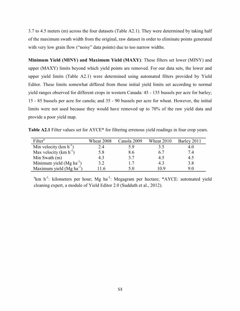
53

3.7 to 4.5 meters (m) across the four datasets (Table A2.1). They were determined by taking half

of the maximum swath width from the original, raw dataset in order to eliminate points generated

with very low grain flow (“noisy” data points) due to too narrow widths.

Minimum Yield (MINY) and Maximum Yield (MAXY): These filters set lower (MINY) and

upper (MAXY) limits beyond which yield points are removed. For our data sets, the lower and

upper yield limits (Table A2.1) were determined using automated filters provided by Yield

Editor. These limits somewhat differed from those initial yield limits set according to normal

yield ranges observed for different crops in western Canada: 45 - 135 bussels per acre for barley;

15 - 85 bussels per acre for canola; and 35 - 90 bussels per acre for wheat. However, the initial

limits were not used because they would have removed up to 70% of the raw yield data and

provide a poor yield map.

Table A2.1 Filter values set for AYCE* for filtering errenous yield readings in four crop years.

Filtera Wheat 2008 Canola 2009 Wheat 2010 Barley 2011

Min velocity (km h-1

) 2.4 5.9 3.5 4.0

Max velocity (km h-1

) 5.8 8.6 6.7 7.4

Min Swath (m) 4.3 3.7 4.5 4.5

Minimum yield (Mg ha-1

) 3.2 1.7 4.3 3.8

Maximum yield (Mg ha-1

) 11.6 5.0 10.9 9.0

akm h

-1: kilometers per hour; Mg ha

-1: Megagram per hectare; *AYCE: automated yield

cleaning expert, a module of Yield Editor 2.0 (Sudduth et al., 2012).

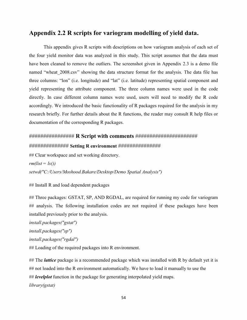
54

Appendix 2.2 R scripts for variogram modelling of yield data.

This appendix gives R scripts with descriptions on how variogram analysis of each set of

the four yield monitor data was analyzed in this study. This script assumes that the data must

have been cleaned to remove the outliers. The screenshot given in Appendix 2.3 is a demo file

named “wheat_2008.csv” showing the data structure format for the analysis. The data file has

three columns: “lon” (i.e. longitude) and “lat” (i.e. latitude) representing spatial component and

yield representing the attribute component. The three column names were used in the code

directly. In case different column names were used, users will need to modify the R code

accordingly. We introduced the basic functionality of R packages required for the analysis in my

research briefly. For further details about the R functions, the reader may consult R help files or

documentation of the corresponding R packages.

################ R Script with comments ######################

############## Setting R environment ###############

## Clear workspace and set working directory.

rm(list = ls())

setwd("C:/Users/Moshood.Bakare/Desktop/Demo Spatial Analysis")

## Install R and load dependent packages

## Three packages: GSTAT, SP, AND RGDAL, are required for running my code for variogram

## analysis. The following installation codes are not required if these packages have been

installed previously prior to the analysis.

install.packages("gstat")

install.packages("sp")

install.packages("rgdal")

## Loading of the required packages into R environment.

## The lattice package is a recommended package which was installed with R by default yet it is

## not loaded into the R environment automatically. We have to load it manually to use the

## levelplot function in the package for generating interpolated yield maps.

library(gstat)

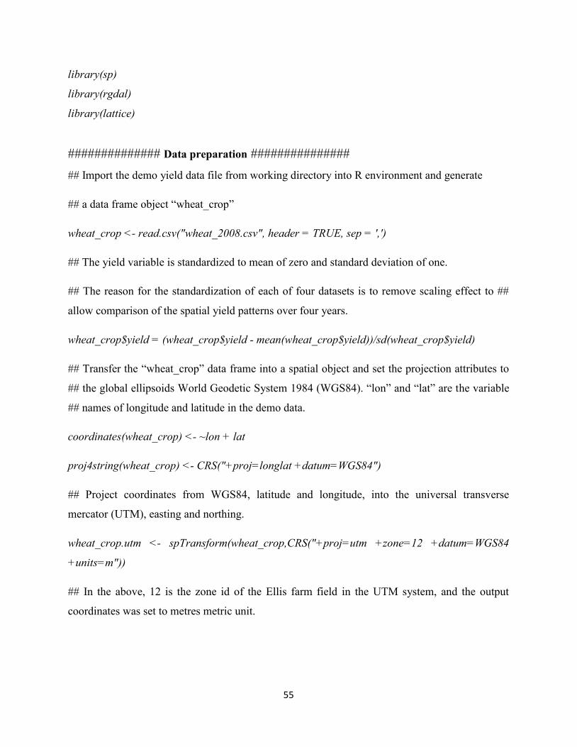
55

library(sp)

library(rgdal)

library(lattice)

############## Data preparation ###############

## Import the demo yield data file from working directory into R environment and generate

## a data frame object “wheat_crop”

wheat_crop <- read.csv("wheat_2008.csv", header = TRUE, sep = ',')

## The yield variable is standardized to mean of zero and standard deviation of one.

## The reason for the standardization of each of four datasets is to remove scaling effect to ##

allow comparison of the spatial yield patterns over four years.

wheat_crop$yield = (wheat_crop$yield - mean(wheat_crop$yield))/sd(wheat_crop$yield)

## Transfer the “wheat_crop” data frame into a spatial object and set the projection attributes to

## the global ellipsoids World Geodetic System 1984 (WGS84). “lon” and “lat” are the variable

## names of longitude and latitude in the demo data.

coordinates(wheat_crop) <- ~lon + lat

proj4string(wheat_crop) <- CRS("+proj=longlat +datum=WGS84")

## Project coordinates from WGS84, latitude and longitude, into the universal transverse

mercator (UTM), easting and northing.

wheat_crop.utm <- spTransform(wheat_crop,CRS("+proj=utm +zone=12 +datum=WGS84

+units=m"))

## In the above, 12 is the zone id of the Ellis farm field in the UTM system, and the output

coordinates was set to metres metric unit.

56

##################### Variogram modelling ################################

## Compute isotropic empirical variogram for the yield attribute from spatial object

wheat_crop.utm.

empvar <- variogram(yield~1, wheat_crop.utm, cutoff = 300, width = 5, cressie = TRUE)

## The expression yield~1 indicates that y ie ld is a response variable, and 1 means no covariate

## to be considered in the analysis. The distance intervals into which point pairs were grouped

## for an estimate of semivariance was 5 metres as indicated by width = 5. The maximum

## distance to be considered in the analysis is 300 metres as given by cutoff = 300.

## I set the cressie argument to a logical value of TRUE to calculate robust empirical variogram

## with estimators that alleviate the effect of spatial outliers as proposed by

## Cressie and Hawkins (1980).

## Visualization of empirical variogram plot

plot(empvar, xlab = "Lag distance (m)", ylab = "Semivariance", main = "Empirical variogram

plot of yield")

## Estimate initial values of partial sill, range, and nugget parameters from the empirical

variogram output empvar.

nr = nrow(empvar)

range = mean(empvar$dist[1 : round(0.2 * nr)])

nugget = mean(empvar$gamma[1 : round(0.05 * nr)])

psill = mean(empvar$gamma[round(0.8 * nr) : nr])-nugget

## Generate variogram models with model types – “Sph” (Spherical),

## “Gau” (Gaussian), and “Exp” (Exponential) by using the above initial values of

## psill (partial sill), range, and nugget.

57

sph.var <- vgm(psill, model = "Sph", range, nugget)

gau.var <- vgm(psill, model = "Gau", range, nugget)

exp.var <- vgm(psill, model = "Exp", range, nugget)

## Fit the empirical variogram (empvar) by using the variogram models

## (sph.var, gau.var, and exp.var) generated from the vgm function.

sph.mod <- fit.variogram(empvar, sph.var, fit.sills = TRUE, fit.ranges = TRUE, fit.method = 7)

gau.mod <- fit.variogram(empvar, gau.var, fit.sills = TRUE, fit.ranges = TRUE, fit.method = 7)

exp.mod <- fit.variogram(empvar, exp.var, fit.sills = TRUE, fit.ranges = TRUE, fit.method = 7)

## Both fit.sills and fit.ranges arguments were assigned the default logical values of TRUE to

## require the fit.variogram function to estimate the psill and range using the empirical

## variogram. We fitted the spatial models using the fitting method proposed by Cressie (1993),

## or fit.method = 7, known as a weighted least-squares (WLS) algorithm that uses weights

## 2/

hN h , in which

hN is the number of point pairs and h is the distance. See Appendix 2.4 for

## other methods used by GSTAT for fitting variogram models.

## Display parameters of fitted variogram model

print(sph.mod)

print(gau.mod)

print(exp.mod)

58

#### Plot the empirical variogram and the fitted spatial models #######

## Plot the fitted variogram models and empirical variogram on a single plot for the assessment

of goodness-of-fit

plot_colors <- c("red", "blue", "green")

xlim = range(c(0, empvar$dist))

ylim = range(c(0, empvar$gamma))

## Open a png file for outputting figures

png(file = "omnidirecvar_2008.png", width = 600, height = 500)

plot(gamma~dist, empvar, xlim = xlim, ylim = ylim, col = 'black', ylab = 'Semivariance', xlab =

'Lag distance (m)', cex = 0.7)

## Add curves for the fitted variogram models to the plot

lines(variogramLine(exp.mod, 300, min = 0.03), lty = 1, col = plot_colors[1], lwd = 1)

lines(variogramLine(gau.mod, 300, min = 0.03), lty = 2, col = plot_colors[2], lwd = 1)

lines(variogramLine(sph.mod, 300, min = 0.03), lty = 3, col = plot_colors[3], lwd = 1)

# Create a legend in the bottom-right corner that is slightly smaller and has no border

legend("bottomright", c("Exp", "Gau", "Sph"), col = plot_colors, lty = 1:3, ncol = 3, bty = "n")

## Save the png file

dev.off()

#### Assess goodness-of-fit of fitted models to empirical variogram ####

## Assess the goodness-of-fit of each fitted model to the empirical variogram by examining its

## weighted sum of squares error (SSErr) statistics.

SSErr.mod <- numeric(3)

59

names(SSErr.mod) <- c("Spherical", "Gaussian", "Exponential")

SSErr.mod[1] = attr(sph.mod, "SSErr")

SSErr.mod[2] = attr(gau.mod, "SSErr")

SSErr.mod[3] = attr(exp.mod, "SSErr")

## Print out the SSErr statistics values for the three fitted models

print(SSErr.mod)

## The exponential model was suggested as optimal for the Ellis Farm data as it has the least

SSErr estimate.

#### Assess the predictability of the fitted models by cross validation #########

## The 5-fold cross validation was used to determine the prediction accuracy of the fitted

## models. Each dataset was randomly partitioned into five subsets out of which four subsets

## were used in training the model and the remaining subset in validating the model. For the

## yield observations in the validating subset, local kriging was performed based on maximum

## of 20 nearest neighbors from the training subsets and the coordinates of the observations in

## the validating data.

sph.kcv <- krige.cv(yield ~ 1, wheat_crop.utm, model = sph.mod, nmax = 20, nfold = 5)

gau.kcv <- krige.cv(yield ~ 1, wheat_crop.utm, model = gau.mod, nmax = 20, nfold = 5)

exp.kcv <- krige.cv(yield ~ 1, wheat_crop.utm, model = exp.mod, nmax = 20, nfold = 5)

## Calculate the root of mean square error (RMSE) from the output of cross validation (krige.cv)

## as diagnostic statistics to identify the optimal model with good prediction accuracy among the

## fitted models. The model which provide the least RMSE was suggested as optimal in this

## study.

60

rmse.mod <- numeric(3)

names(rmse.mod) <- c("Spherical", "Gaussian", "Exponential")

rmse.mod[1] <- sqrt(mean(sph.kcv$residual ^ 2))

rmse.mod[2] <- sqrt(mean(gau.kcv$residual ^ 2))

rmse.mod[3] <- sqrt(mean(exp.kcv$residual ^ 2))

## Print out the RMSE statistics values for the three fitted models

print(rmse.mod)

## Calculate the correlation coefficient of the observed and predicted values from cross

## cross validation with other diagnostic statistics to identify the optimal prediction model

cor.mod <- numeric(3)

names(cor.mod) <- c("Spherical","Gaussian","Exponential")

cor.mod[1] <- cor(sph.kcv$observed, sph.kcv$observed - sph.kcv$residual)

cor.mod[2] <- cor(gau.kcv$observed, gau.kcv$observed - gau.kcv$residual)

cor.mod[3] <- cor(exp.kcv$observed, exp.kcv$observed - exp.kcv$residual)

## Print out the correlation coefficient values for the three fitted models

print(cor.mod)

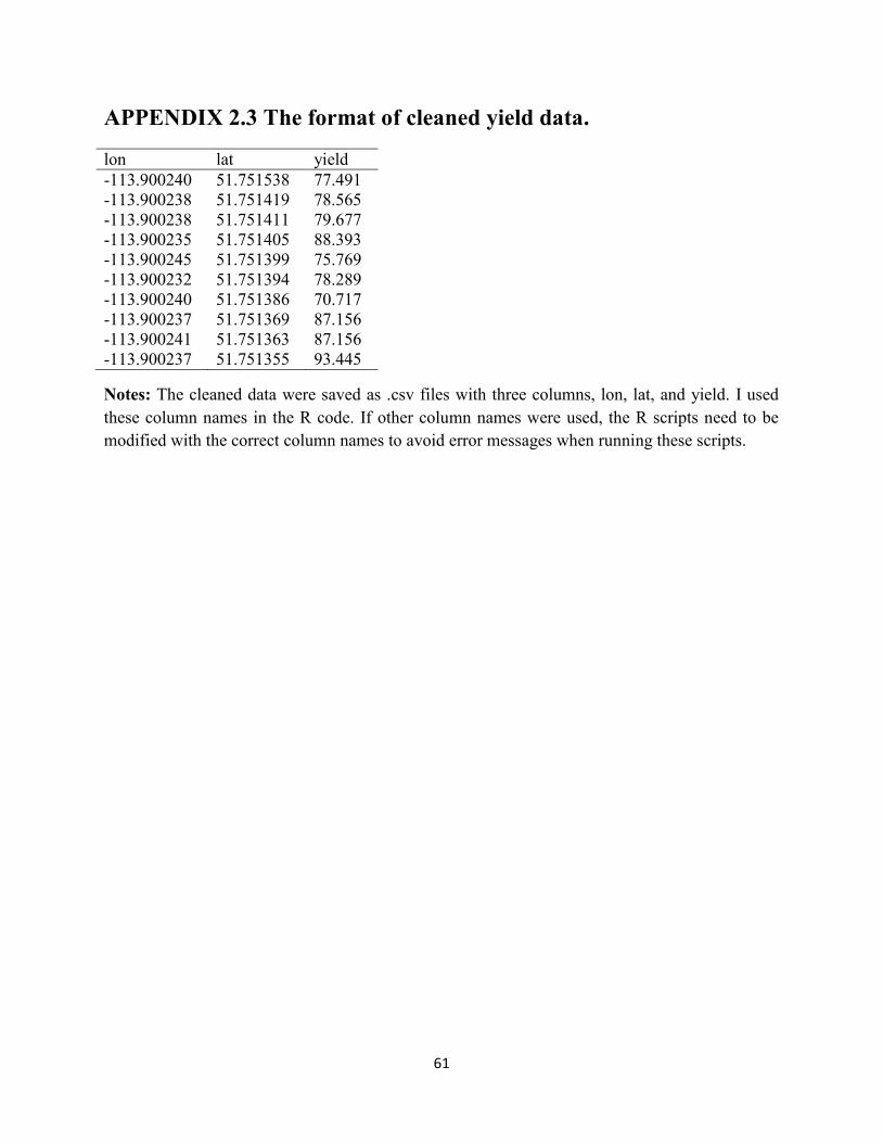
61

APPENDIX 2.3 The format of cleaned yield data.

lon lat yield

-113.900240 51.751538 77.491

-113.900238 51.751419 78.565

-113.900238 51.751411 79.677

-113.900235 51.751405 88.393

-113.900245 51.751399 75.769

-113.900232 51.751394 78.289

-113.900240 51.751386 70.717

-113.900237 51.751369 87.156

-113.900241 51.751363 87.156

-113.900237 51.751355 93.445

Notes: The cleaned data were saved as .csv files with three columns, lon, lat, and yield. I used

these column names in the R code. If other column names were used, the R scripts need to be

modified with the correct column names to avoid error messages when running these scripts.

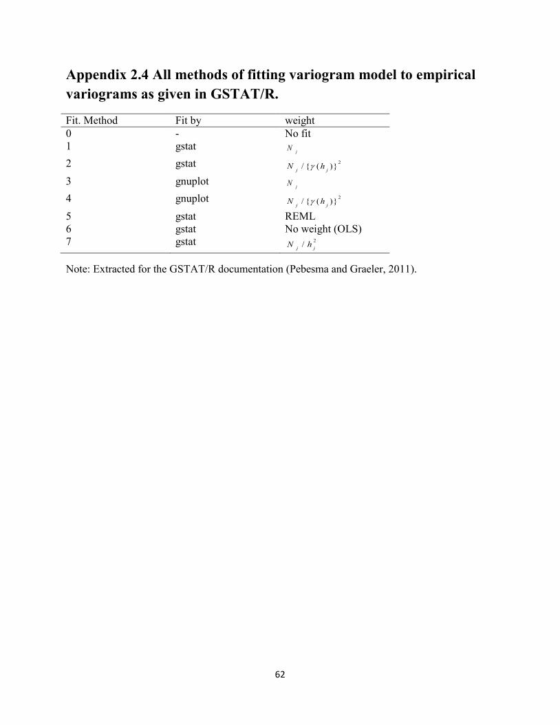
62

Appendix 2.4 All methods of fitting variogram model to empirical

variograms as given in GSTAT/R.

Fit. Method Fit by weight

0 - No fit

1 gstat j

N

2 gstat 2/ { ( )}

j jN h

3 gnuplot j

N

4 gnuplot 2/ { ( )}

j jN h

5 gstat REML

6 gstat No weight (OLS)

7 gstat 2/

j jN h

Note: Extracted for the GSTAT/R documentation (Pebesma and Graeler, 2011).

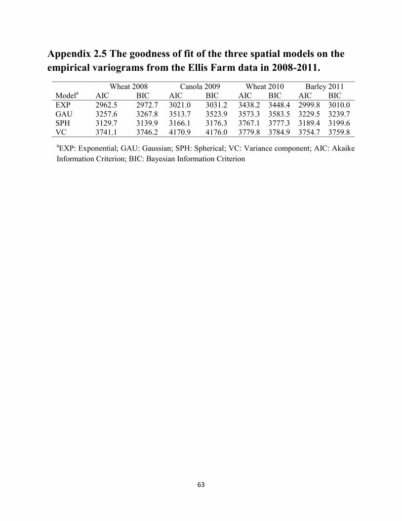
63

Appendix 2.5 The goodness of fit of the three spatial models on the

empirical variograms from the Ellis Farm data in 2008-2011.

Wheat 2008 Canola 2009 Wheat 2010 Barley 2011

Modela AIC BIC AIC BIC AIC BIC AIC BIC

EXP 2962.5 2972.7 3021.0 3031.2 3438.2 3448.4 2999.8 3010.0

GAU 3257.6 3267.8 3513.7 3523.9 3573.3 3583.5 3229.5 3239.7

SPH 3129.7 3139.9 3166.1 3176.3 3767.1 3777.3 3189.4 3199.6

VC 3741.1 3746.2 4170.9 4176.0 3779.8 3784.9 3754.7 3759.8

aEXP: Exponential; GAU: Gaussian; SPH: Spherical; VC: Variance component; AIC: Akaike

Information Criterion; BIC: Bayesian Information Criterion

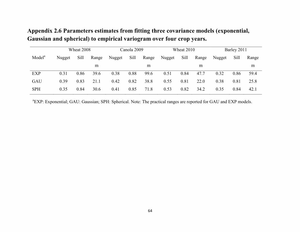
64

Appendix 2.6 Parameters estimates from fitting three covariance models (exponential,

Gaussian and spherical) to empirical variogram over four crop years.

Wheat 2008 Canola 2009 Wheat 2010 Barley 2011

Modela Nugget Sill Range

m

Nugget Sill Range

m

Nugget Sill Range

m

Nugget Sill Range

m

EXP 0.31 0.86 39.6 0.38 0.88 99.6 0.51 0.84 47.7 0.32 0.86 59.4

GAU 0.39 0.83 21.1 0.42 0.82 38.8 0.55 0.81 22.0 0.38 0.81 25.8

SPH 0.35 0.84 30.6 0.41 0.85 71.8 0.53 0.82 34.2 0.35 0.84 42.1

aEXP: Exponential; GAU: Gaussian; SPH: Spherical. Note: The practical ranges are reported for GAU and EXP models.

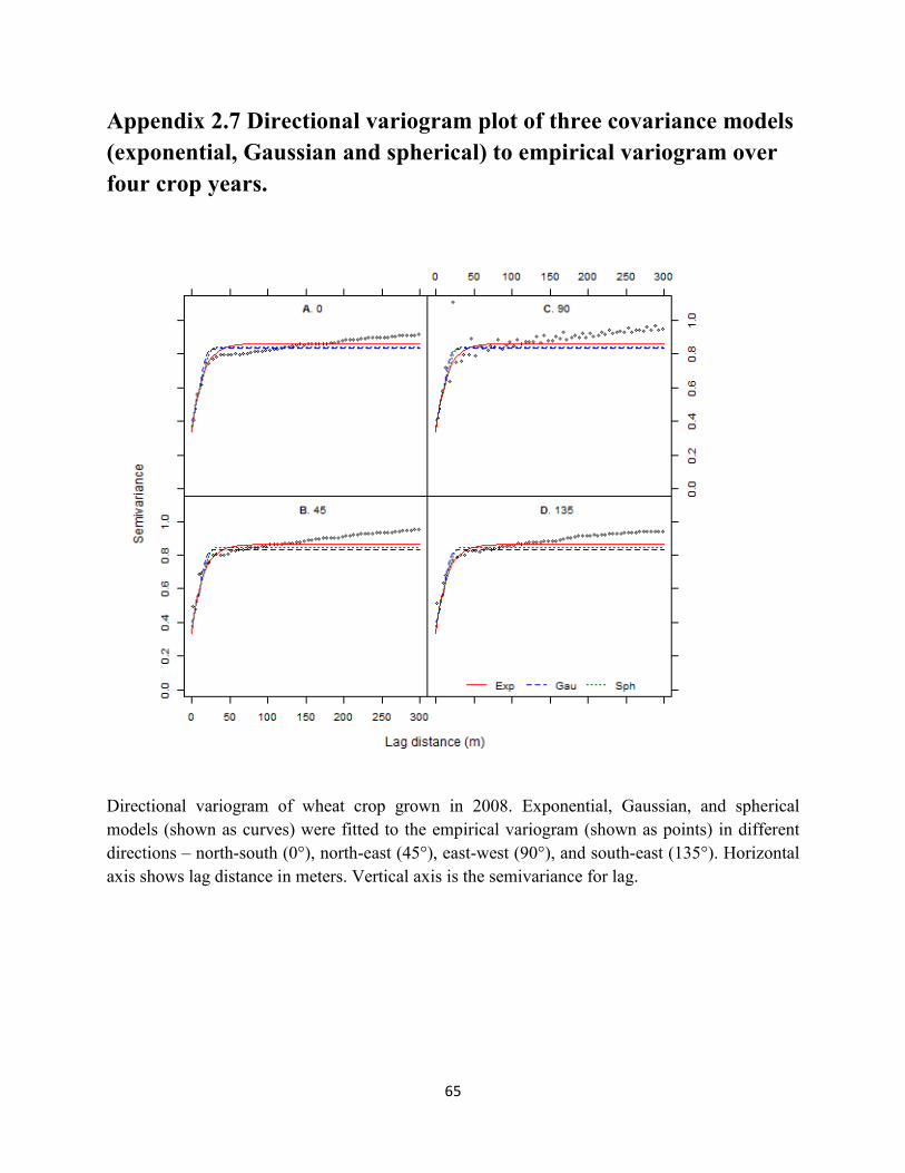
65

Appendix 2.7 Directional variogram plot of three covariance models

(exponential, Gaussian and spherical) to empirical variogram over

four crop years.

Directional variogram of wheat crop grown in 2008. Exponential, Gaussian, and spherical

models (shown as curves) were fitted to the empirical variogram (shown as points) in different

directions – north-south (0°), north-east (45°), east-west (90°), and south-east (135°). Horizontal

axis shows lag distance in meters. Vertical axis is the semivariance for lag.

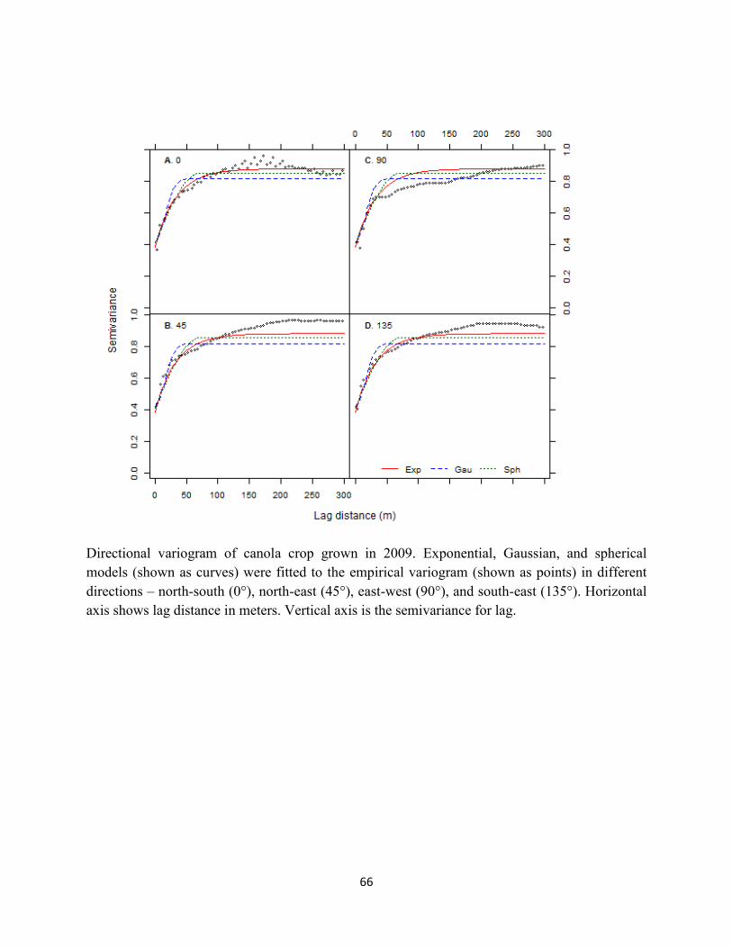
66

Directional variogram of canola crop grown in 2009. Exponential, Gaussian, and spherical

models (shown as curves) were fitted to the empirical variogram (shown as points) in different

directions – north-south (0°), north-east (45°), east-west (90°), and south-east (135°). Horizontal

axis shows lag distance in meters. Vertical axis is the semivariance for lag.

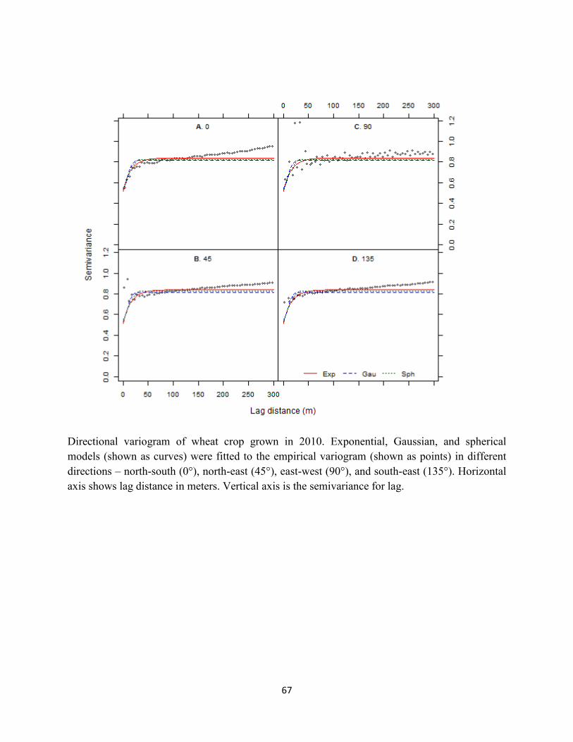
67

Directional variogram of wheat crop grown in 2010. Exponential, Gaussian, and spherical

models (shown as curves) were fitted to the empirical variogram (shown as points) in different

directions – north-south (0°), north-east (45°), east-west (90°), and south-east (135°). Horizontal

axis shows lag distance in meters. Vertical axis is the semivariance for lag.

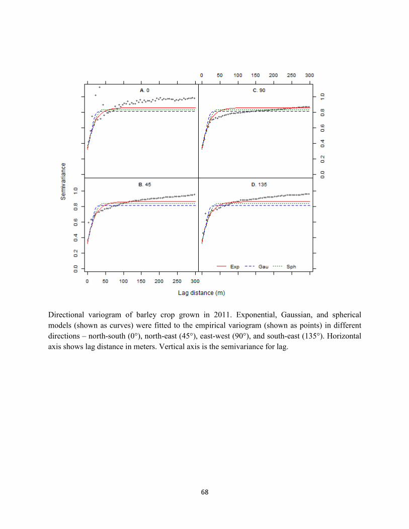
68

Directional variogram of barley crop grown in 2011. Exponential, Gaussian, and spherical

models (shown as curves) were fitted to the empirical variogram (shown as points) in different

directions – north-south (0°), north-east (45°), east-west (90°), and south-east (135°). Horizontal

axis shows lag distance in meters. Vertical axis is the semivariance for lag.

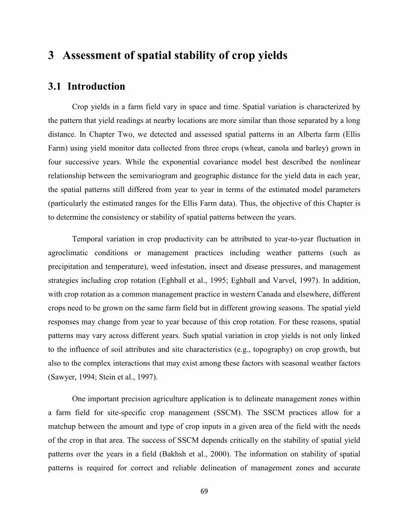
69

3 Assessment of spatial stability of crop yields

3.1 Introduction

Crop yields in a farm field vary in space and time. Spatial variation is characterized by

the pattern that yield readings at nearby locations are more similar than those separated by a long

distance. In Chapter Two, we detected and assessed spatial patterns in an Alberta farm (Ellis

Farm) using yield monitor data collected from three crops (wheat, canola and barley) grown in

four successive years. While the exponential covariance model best described the nonlinear

relationship between the semivariogram and geographic distance for the yield data in each year,

the spatial patterns still differed from year to year in terms of the estimated model parameters

(particularly the estimated ranges for the Ellis Farm data). Thus, the objective of this Chapter is

to determine the consistency or stability of spatial patterns between the years.

Temporal variation in crop productivity can be attributed to year-to-year fluctuation in

agroclimatic conditions or management practices including weather patterns (such as

precipitation and temperature), weed infestation, insect and disease pressures, and management

strategies including crop rotation (Eghball et al., 1995; Eghball and Varvel, 1997). In addition,

with crop rotation as a common management practice in western Canada and elsewhere, different

crops need to be grown on the same farm field but in different growing seasons. The spatial yield

responses may change from year to year because of this crop rotation. For these reasons, spatial

patterns may vary across different years. Such spatial variation in crop yields is not only linked

to the influence of soil attributes and site characteristics (e.g., topography) on crop growth, but

also to the complex interactions that may exist among these factors with seasonal weather factors

(Sawyer, 1994; Stein et al., 1997).

One important precision agriculture application is to delineate management zones within

a farm field for site-specific crop management (SSCM). The SSCM practices allow for a

matchup between the amount and type of crop inputs in a given area of the field with the needs

of the crop in that area. The success of SSCM depends critically on the stability of spatial yield

patterns over the years in a field (Bakhsh et al., 2000). The information on stability of spatial

patterns is required for correct and reliable delineation of management zones and accurate

70

estimation of input amounts and associated costs. Recent studies have given priority to the use of

management zones as a means to more effectively apply variable rate technology (VRT) across

fields (Ferguson et al., 2003). A number of studies have reported the use of geostatistical

analyses for defining the management zones of site-specific crop inputs (Cressie, 1993; Griffin,

2010; Oliver, 2010; Stein and Corsten, 1991). However, there is little or no discussion on the

assessment of the stability of spatial yield patterns across the years and its use for delineating

management zones within a field.

In this chapter we will describe a geostatistical method that allows for assessment of the

stability of yield patterns across the years. The same data sets used in Chapter Two will be used

to illustrate the application of this method.

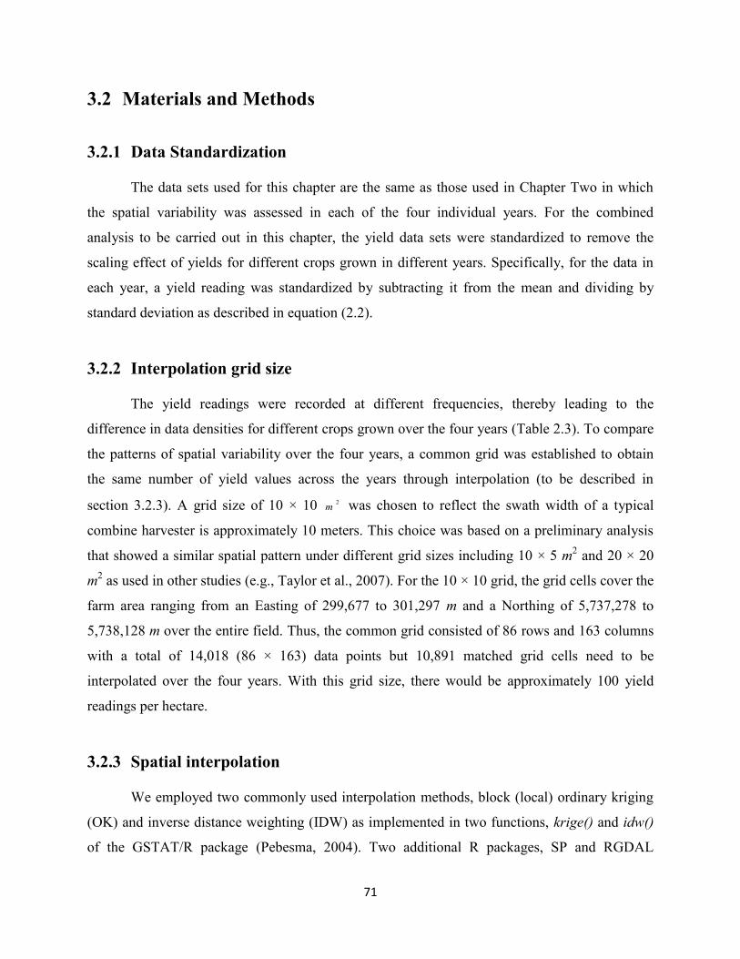
71

3.2 Materials and Methods

3.2.1 Data Standardization

The data sets used for this chapter are the same as those used in Chapter Two in which

the spatial variability was assessed in each of the four individual years. For the combined

analysis to be carried out in this chapter, the yield data sets were standardized to remove the

scaling effect of yields for different crops grown in different years. Specifically, for the data in

each year, a yield reading was standardized by subtracting it from the mean and dividing by

standard deviation as described in equation (2.2).

3.2.2 Interpolation grid size

The yield readings were recorded at different frequencies, thereby leading to the

difference in data densities for different crops grown over the four years (Table 2.3). To compare

the patterns of spatial variability over the four years, a common grid was established to obtain

the same number of yield values across the years through interpolation (to be described in

section 3.2.3). A grid size of 10 × 10 2m was chosen to reflect the swath width of a typical

combine harvester is approximately 10 meters. This choice was based on a preliminary analysis

that showed a similar spatial pattern under different grid sizes including 10 × 5 m2 and 20 × 20

m2 as used in other studies (e.g., Taylor et al., 2007). For the 10 × 10 grid, the grid cells cover the

farm area ranging from an Easting of 299,677 to 301,297 m and a Northing of 5,737,278 to

5,738,128 m over the entire field. Thus, the common grid consisted of 86 rows and 163 columns

with a total of 14,018 (86 × 163) data points but 10,891 matched grid cells need to be

interpolated over the four years. With this grid size, there would be approximately 100 yield

readings per hectare.

3.2.3 Spatial interpolation

We employed two commonly used interpolation methods, block (local) ordinary kriging

(OK) and inverse distance weighting (IDW) as implemented in two functions, krige() and idw()

of the GSTAT/R package (Pebesma, 2004). Two additional R packages, SP and RGDAL

72

packages, were also used for data preparation with the GSTAT/R analysis. The SP package

provides a set of tools for defining, importing/exporting, and visualization of spatial objects. The

RGDAL package is required not only for reading spatial data from various formats into the R

workspace but also for transforming the spatial data from one coordinate reference system to

another. R code along with detailed comments is given in Appendix 3.1.

We created the coordinates of the interpolation grid by employing a 10 m cell size that

covers the entire study field from an easting and northing direction. Thus, we established a

common grid for interpolation using an R function expand.grid(). The interpolation grid was

converted to gridded spatial object and expressed on the same coordinate reference system as

that of the sampled data. Given that the observed yield readings in each crop year were not

strictly equally spaced, a search window of 10 to 20 observations per interpolated data yield

point was used as the neighboorhood size. This neighborhood size was considered an appropriate

balance between having enough information borrowed from nearest neighbors and the amount of

noise introduced from distant neighbors. The interpolated yield values were block-averaged to

400 m square cells as specified by argument block = c(20,20). Similarly, the IDW interpolation

method was done in the same manner using the idw() function but with power of 2 specified

through the idp argument to indicate the squared geographic distance separating the data points.

Regardless of the OK or IDW interpolation, each gridded point was estimated as a

weighted average of sampled (observed) data in a neighborhood. The estimation formula is given

by:

(3.1)

where is the estimated (interpolated) yield at unknown location, ; is a number of sample

data points in the local neighborhood for the estimation of ; is the weight assigned to the

ith neighboring sample value, ( )i

z u is the observed yield at location (Webster and Oliver,

2001). Summing all weights to one in equation (3.1) allows for a quick assessment of the relative

0

1

1

ˆ  

1

n

i i

i

n

i

i

z u z u

z 0u n

0ˆ ( )z u

i

iu

73

contribution by each known value to the estimation of the unobserved value. The weight

(relative importance) of each known value to the unknown value (to be interpolated) was

determined according to interpolation methods. The weight for the IDW method was calculated

as the reciprocal of the squared distance between the known and the unknown yields whereas the

weight for the OK method was derived from the covariance function (the exponential covariance

function as identified in Chapter Two) describing the spatial correlations between known and

unknown yield readings and among known yield readings themselves (Isaaks and Srivastava,

1989; Wong et al., 2004).

3.2.4 Assessment of stability of yield patterns

The resulting interpolated yield values as obtained from the two interpolation methods (OK and

IDW) were converted to a data frame object and exported to a text file. The stability of spatial

yield patterns over the four years was assessed in two ways. First, yield maps from the

interpolated data over the four years were produced and visually examined. Second, Pearson’s

correlation coefficient, r, between pairs of the four years were computed using SAS PROC

CORR (SAS Institute Inc, 2014).

74

3.3 Results

Summary statistics of interpolated yield values from the common grid permits

comparison of the four spatial yield distributions in the four crop years (Table 3.1). These were

somewhat different from those based on cleaned, but non-interpolated yield data where the

number of yield readings varied from year to year as described in Chapter Two. There were

significant correlation coefficients between interpolated yield values obtained from the OK or

IDW interpolation between six pairs of the years (Tables 3.2 and 3.3). However, these significant

correlations were generally low to moderate, ranging from 0.18 for the year pair of canola-2009

and wheat-2010; to 0.37 for the year pair of wheat-2010 and barley-2011. In comparison to

correlation coefficients of interpolated yield values obtained with the OK method, the

correlations from the IDW method were very similar, ranging from 0.18 for the year pair of

canola-2009 and wheat-2010; to 0.37 for the year pair of wheat-2010 and barley-2011 (Table

3.3). Table 3.4 presents weighted sum of squares error (SSErr) as a goodness-of-fit statistic of

fitted models to the variogram of interpolated yield values resulting from the OK method. The

results showed that exponential model had the least value of SSErr and it would be considered to

be the most appropriate model to best describe the spatial variability of yield in this farm field.

The normalized yield maps of block kriged predictions for year 2008 to 2011 are

presented in Figure 3.1 using cleaned yields and geostatistical parameters (range, nugget and

partial sill) from the exponential model as identified in Chapter Two. Similarly, Figure 3.2

showed the resulting yield maps based on the IDW method which were visually similar to those

obtained from the OK method for the yield data in each crop year. In each case, the yield scale

on the maps was based on a normalized score of yield from that year. This permits visual

assessment of the spatial yield patterns over the years.

Visual inspection of four yield maps from this farm field using OK and IDW

interpolations (Figures 3.1 and 3.2) revealed little stability in yield patterns over the years. This

observation was confirmed by the low correlation coefficients (Table 3.2 and 3.3). As seen in

Figure 3.1 or Figure 3.2, few patches of high yielding areas were noticeable in wheat 2008 while

the rest of the field showed predominantly low yield while in canola 2009, predominantly low

yields were evident in the north and north-east region of the field except a few patches with high

75

yield. Wheat-2010 yield maps had a noticeable patch of high yield in the north region and

various patches of low yield in other areas of the field compared to barley 2011 yield maps that

had relatively similar patterns as wheat-2010 but showed a patch of high yield in the east-west

direction. There was a tendency of consistently lower yields in the north-west region of the field

as observed for all crop-years.

Variogram plots of interpolated yield values and fitted models were provided (Figures 3.3

to 3.6). The visualization of these plots revealed that the exponential covariance model would be

an appropriate model to best fit and capture the spatial variability of interpolated yield values

across the four years. This is further confirmed from assessment of goodnes-of-fit of the fitted

models to interpolated yield values with the exponential function having the least values of

SSErr statistics as shown in Table 3.4.

76

3.4 Discussion

Crop yield is the ultimate ‘product’ of landscape and climatic variability in a farm field

and consequently should provide useful information to identify management zones for optimal

crop productivity. However, with year-to-year variation in agroclimatic/adaphic conditions and

agronomic practices applied to the field, it is difficult to identify useful management zones based

on a single year’s yield map. The present chapter addressed this issue by a combined analysis of

four data sets from the same field. With three crops (wheat, canola and barley) being rotated in

four years (2008-2011) and yield readings being recorded in different densities for different crop

years, our combined analysis consists of (i) standardizing the yield data in individual years; (ii)

interpolating those yields under a common grid imposed over all four years; and (iii) comparing

the yield maps over the years and computing correlations between the interpolated yield pairs

over the years to assess the stability of spatial yield patterns.

Our results showed a low level of spatial stability between the years. Similar findings

were reported in earlier studies (Bakhsh et al., 2000; Lamb et al., 1997). Lamb et al. (1997)

found a lack of spatial stability of corn grain yields collected over five years. Bakhsh et al.

(2000) also observed a lack of spatial stability of corn/soybean yields collected over three years

(1995-1997) from a 25 ha field located near Story City, Iowa. The instability of spatial yield

patterns observed in our study and other studies indicates low predictive capability in the field. In

other words, yield prediction in subsequent years using yields from one or more previous years is

unreliable. This unreliability creates difficulty when identifying the low- or high-yield zones

within a field that are consistent over the years that are required for site-specific crop

management.

Our analysis is different from other approaches in addressing the problem. Kleinjan et al.

(2007) described a method of identifying productivity zones in a farm field. Like our procedure,

their procedure involves removing erroneous data or “cleaning” the yield data sets and creating

common grid cells across years. However, unlike our procedure, these authors calculated yield

and standard deviation maps. They created “Average” yield maps from multiple years of yield

monitor data for determining yield goals and fertilizer recommendations, while they used

standard deviation maps to identify areas requiring corrective management. In their application

77

to the analysis of corn yield data collected in four years (1996, 1998, 2000 and 2002), the yield

variability in productivity zones that incorporated both standard deviation and average yield data

was, on average, 43% lower than total field variability over four years. Obviously, their method

did not account for the presence of spatial correlation when calculating the mean yield and

standard deviation from a neighboring area. Rodrigues et al. (2013) described a mixed-model

approach to the analysis of multi-year georeferenced corn yield and soil data at a study site (10

by 250 m) located in São Paulo State, Brazil. While their statistical models were able to account

for heteroscedastic and spatial-temporal autocorrelation, their data sets in individual years were

small enough (n < 1,000) so that the commonly used statistical software packages such as SAS

PROC MIXED (SAS Institute Inc, 2014) were capable of handling. However, a typical yield

monitor data set would be in the order of 50,000 to 100,000 yield readings. This is far beyond the

computing capacity of most statistical software packages even with our current powerful

computers. For this reason, we have used a weighted least squares method as implemented in the

GSTAT/R package (Pebesma and Graeler, 2011) to carry out the nonlinear regression of

empirical semivariograms on distances that would be computationally less demanding.

Our method of assessing the spatial stability was limited to the correlation between a pair

of years at a time. It would be desirable to assess the spatial stability over multiple years

simultaneously. One approach to carry out the mixed-model analysis is to obtain the likelihood-

based fit statistics and subsequently a likelihood ratio test can be calculated by comparing a full

model (spatial heterogeneity across the years) and a reduced model (spatial homogeneity across

the years). However, the usual implementation of the mixed-model analysis (e.g., Rodrigues et

al., 2013) remains computationally infeasible with large data sets like those in our study. Thus a

more efficient algorithm is definitely needed to alleviate the computing burden arising from

variogram calculation and interpolation through kriging or inverse distance methods.

78

3.5 Summary and Conclusions

Filtered and standardized yield monitor data from four years (2008-2011) were analyzed

for an understanding of the spatial stability of yields across a crop field production. Wheat,

canola, and barley were grown during the study period, and different herbicide, fungicide and

fertilizer rates were applied with variation in climatic factors. In order to assess the spatial

stability of yield patterns over different crop years, data were standardized and interpolated on a

common grid using ordinary block kriging and inverse squared distance weighting methods.

The extent of spatial stability of yield patterns between pairs of years was assessed by

Pearson’s correlation coefficients. The resulting correlation coefficients were low to moderate

across different year pairs. The results suggest that (i) yield patterns from the production field

were spatially inconsistent between the years; (ii) the interpolated yield maps lack spatial

stability pattern to delineate management zones within the field.

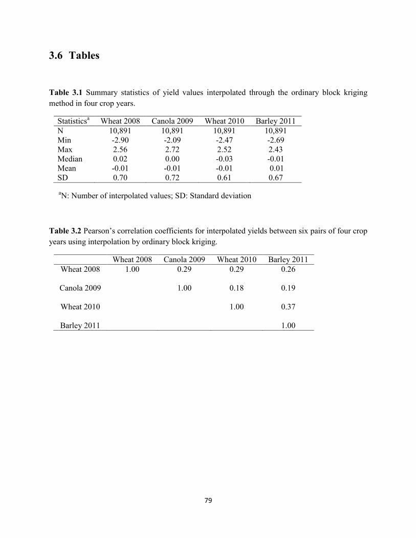
79

3.6 Tables

Table 3.1 Summary statistics of yield values interpolated through the ordinary block kriging

method in four crop years.

Statisticsa Wheat 2008 Canola 2009 Wheat 2010 Barley 2011

N 10,891 10,891 10,891 10,891

Min -2.90 -2.09 -2.47 -2.69

Max 2.56 2.72 2.52 2.43

Median 0.02 0.00 -0.03 -0.01

Mean -0.01 -0.01 -0.01 0.01

SD 0.70 0.72 0.61 0.67

aN: Number of interpolated values; SD: Standard deviation

Table 3.2 Pearson’s correlation coefficients for interpolated yields between six pairs of four crop

years using interpolation by ordinary block kriging.

Wheat 2008 Canola 2009 Wheat 2010 Barley 2011

Wheat 2008 1.00 0.29

0.29

0.26

Canola 2009 1.00 0.18

0.19

Wheat 2010 1.00 0.37

Barley 2011 1.00

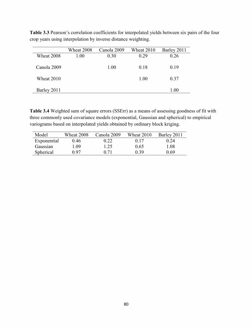
80

Table 3.3 Pearson’s correlation coefficients for interpolated yields between six pairs of the four

crop years using interpolation by inverse distance weighting.

Wheat 2008 Canola 2009 Wheat 2010 Barley 2011

Wheat 2008 1.00 0.30

0.29

0.26

Canola 2009 1.00 0.18

0.19

Wheat 2010 1.00 0.37

Barley 2011 1.00

Table 3.4 Weighted sum of square errors (SSErr) as a means of assessing goodness of fit with

three commonly used covariance models (exponential, Gaussian and spherical) to empirical

variograms based on interpolated yields obtained by ordinary block kriging.

Model Wheat 2008 Canola 2009 Wheat 2010 Barley 2011

Exponential 0.46 0.22 0.17 0.24

Gaussian 1.09 1.25 0.65 1.08

Spherical 0.97 0.71 0.39 0.69

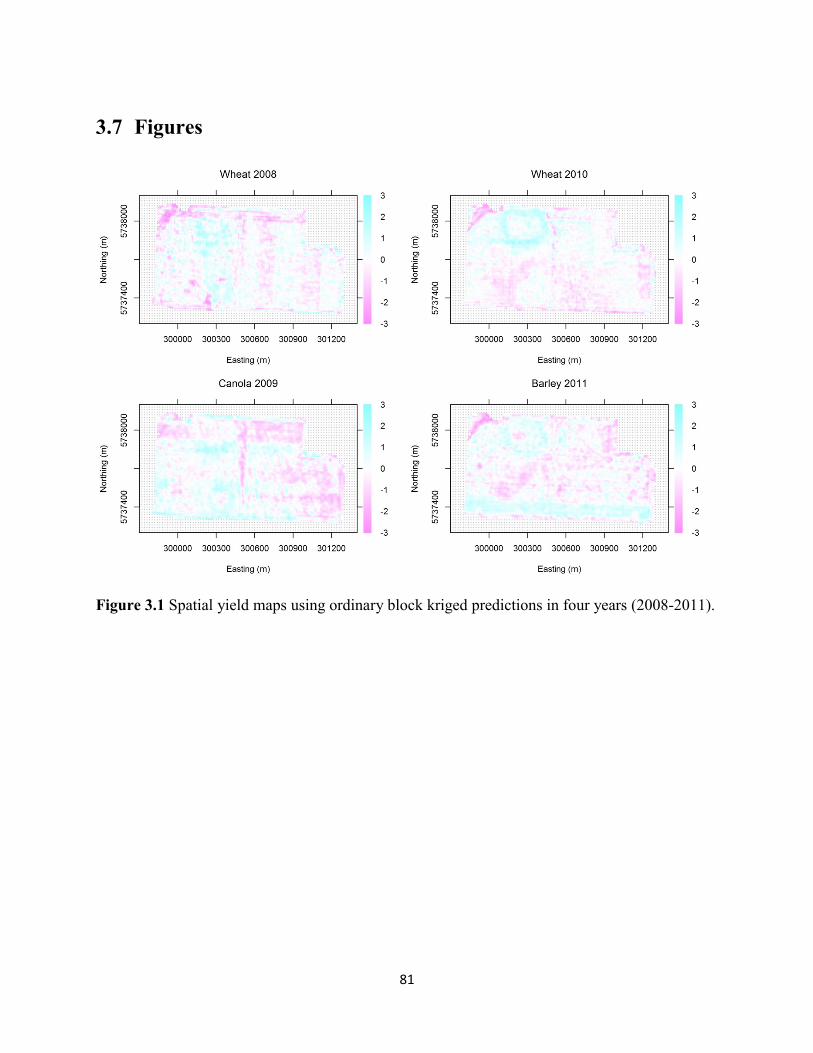
81

3.7 Figures

Figure 3.1 Spatial yield maps using ordinary block kriged predictions in four years (2008-2011).

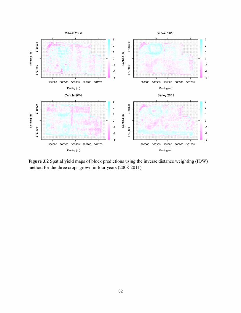
82

Figure 3.2 Spatial yield maps of block predictions using the inverse distance weighting (IDW)

method for the three crops grown in four years (2008-2011).

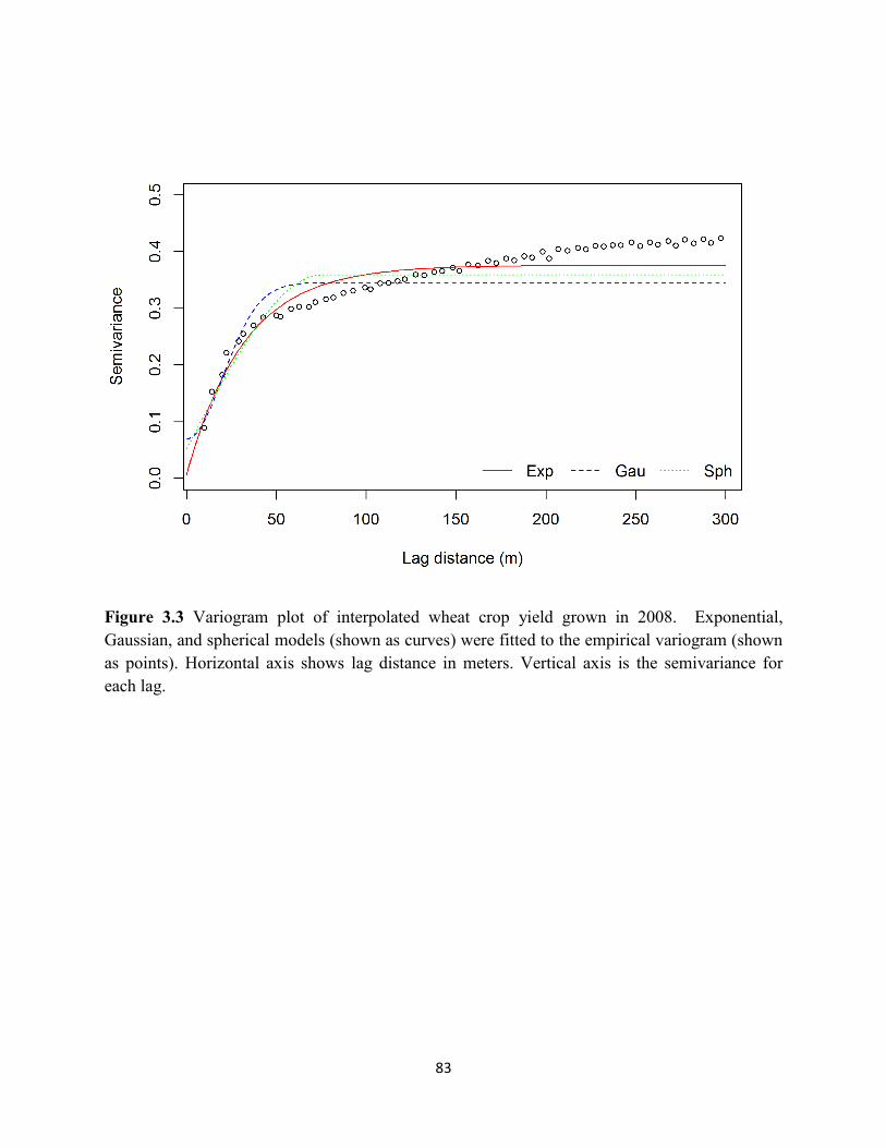
83

Figure 3.3 Variogram plot of interpolated wheat crop yield grown in 2008. Exponential,

Gaussian, and spherical models (shown as curves) were fitted to the empirical variogram (shown

as points). Horizontal axis shows lag distance in meters. Vertical axis is the semivariance for

each lag.

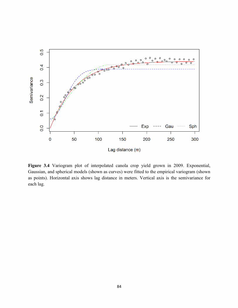
84

Figure 3.4 Variogram plot of interpolated canola crop yield grown in 2009. Exponential,

Gaussian, and spherical models (shown as curves) were fitted to the empirical variogram (shown

as points). Horizontal axis shows lag distance in meters. Vertical axis is the semivariance for

each lag.

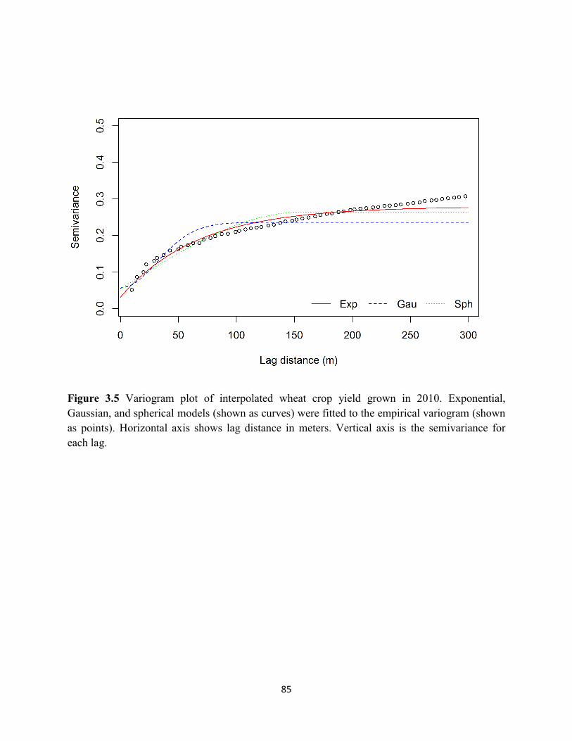
85

Figure 3.5 Variogram plot of interpolated wheat crop yield grown in 2010. Exponential,

Gaussian, and spherical models (shown as curves) were fitted to the empirical variogram (shown

as points). Horizontal axis shows lag distance in meters. Vertical axis is the semivariance for

each lag.

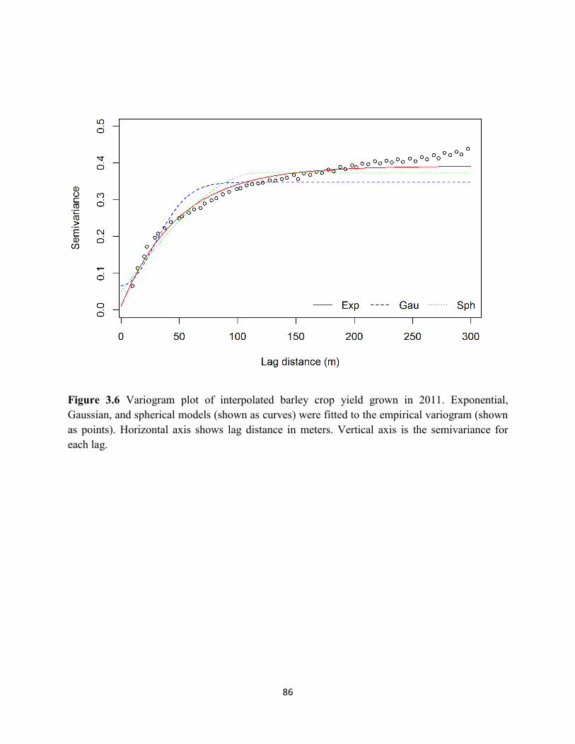
86

Figure 3.6 Variogram plot of interpolated barley crop yield grown in 2011. Exponential,

Gaussian, and spherical models (shown as curves) were fitted to the empirical variogram (shown

as points). Horizontal axis shows lag distance in meters. Vertical axis is the semivariance for

each lag.

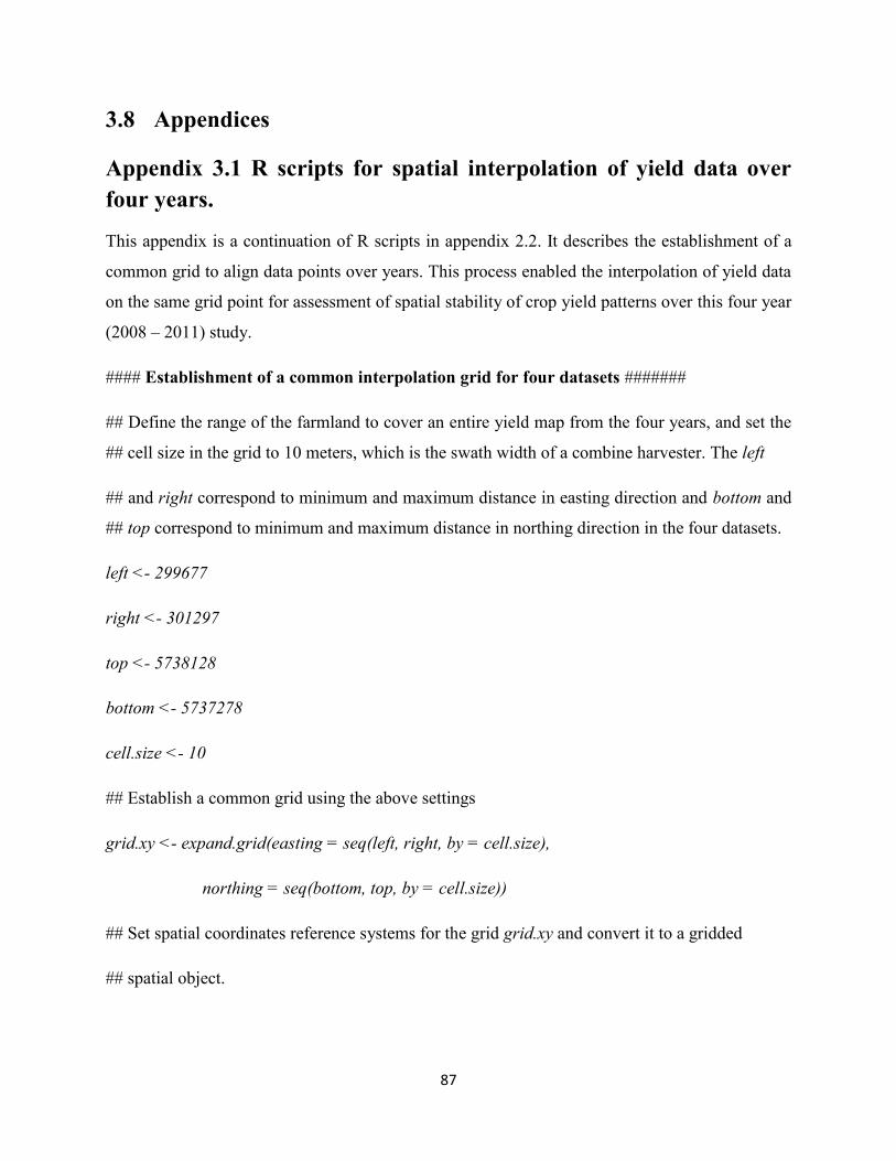
87

3.8 Appendices

Appendix 3.1 R scripts for spatial interpolation of yield data over

four years.

This appendix is a continuation of R scripts in appendix 2.2. It describes the establishment of a

common grid to align data points over years. This process enabled the interpolation of yield data

on the same grid point for assessment of spatial stability of crop yield patterns over this four year

(2008 – 2011) study.

#### Establishment of a common interpolation grid for four datasets #######

## Define the range of the farmland to cover an entire yield map from the four years, and set the

## cell size in the grid to 10 meters, which is the swath width of a combine harvester. The left

## and right correspond to minimum and maximum distance in easting direction and bottom and

## top correspond to minimum and maximum distance in northing direction in the four datasets.

left <- 299677

right <- 301297

top <- 5738128

bottom <- 5737278

cell.size <- 10

## Establish a common grid using the above settings

grid.xy <- expand.grid(easting = seq(left, right, by = cell.size),

northing = seq(bottom, top, by = cell.size))

## Set spatial coordinates reference systems for the grid grid.xy and convert it to a gridded

## spatial object.

88

coordinates(grid.xy) <- ~easting + northing

proj4string(grid.xy) <- CRS("+proj=utm +zone=12 +datum=WGS84 +units=m")

gridded(grid.xy) <- TRUE

## Plot to verify that sample points are within the grid

plot(grid.xy, cex=1.5,col="grey")

points(wheat_crop.utm, pch=1,col="red", cex=0.5)

title("Interpolation Grid and Sample Points")

####### Ordinary Kriging interpolation method #########

## In this study, Ordinary Kriging with an exponential model, being an optimal model that best

## described yield patterns, is used to implement a local kriging of interpolated yield values on

## grid grid.xy within a block size 400 m square cells using a search window of 10 and 20 as the

## minimum and maximum neighborhood size respectively.

## Use a localized ordinary kriging method to interpolate the yields at the intersections of the

## common grid (grid.xy).

yield.krige <- krige(id="yield", yield ~ 1, wheat_crop.utm, grid.xy,

model = exp.mod, nmin = 10, nmax = 20, block = c(20,20))

## The exponential model was used in the interpolation, which was suggested as the optimal

## model for the Ellis Farm data in the previous spatial model comparison of the study. The

## search windows in the kriging were set to 10 and 20 as minimum and maximum

## neighborhood size, respectively.

## create data frame object of interpolated yield values in order to display kriged map

yield.krige <- as.data.frame(yield.krige)

89

## Visualize the interpolated maps in order to examine the stability of spatial-temporal yield

## patterns over the four years.

png(file = "demo_yield_map.png", units = "px", width = 480, height = 480)

print(levelplot(yield.pred ~easting + northing, data = yield.krige, aspect = "iso",

main = "Demo yield map", xlab = "Easting (m)", ylab = "Northing (m)"))

dev.off()

## Write the data frame yield.krige of interpolated yield values into CSV format

write.csv(yield.krige, "demo_kriged_yield.csv", row.names = F)

Having run these R-scripts for each of the four datasets, the interpolated yield values in CSV

format were pooled together to quantitatively assess the stability of spatial yield patterns over

four years. This was carried out by computing Pearson’s correlation coefficient, r, using SAS

PROC CORR (SAS Institute Inc, 2014).

Similarly, the IDW interpolation method was done in the same manner using the idw()

function with power of 2 specified through the idp argument to indicate the squared geographic

distance between the data points. Unlike the Kriging method, it requires no model during the

interpolation.

yield.idw <- idw(yield~1, wheat_crop.utm, grid.xy, nmin = 10, nmax = 20,

block = c(20,20), idp = 2)

90

4 General Discussion and Conclusions

4.1 Introduction

It has long been known that there is spatial variability across a farm field [i.e., the

observed value of the variable (say yield) at one locality is dependent on the values at

neighbouring localities within the field]. However, such variability has been generally ignored as

most farming practices require uniformity as a convenient means of operating modern farm

equipment. Moreover, until recently, the ability to detect and assess in-field spatial variability

has been limited. The situation is now changing with the recent advent of geomatics-based

technologies. These technologies enable the generation of massive crop or soil data across entire

fields with information on geographic locations of the data points being recorded. In this thesis

research, we analyzed the data from one of such technology (yield monitor equipped with GPS)

to detect and assess in-field spatial variability. The focus of our analysis is on investigating the

utility of yield monitor data from a particular farm (Ellis Farm) field located in southern Alberta

for identifying patterns and stability of spatial variability as presented in Chapter Two and

Chapter Three. In this chapter, we summarize the main findings from these two chapters and

discuss implications of the findings for current precision agriculture practices. Furthermore, we

briefly consider limitations of this thesis research and suggest future studies.

4.2 Summary and conclusion

In the first study as reported in chapter 2, we showed that, of the three spatial covariance

models (exponential, Gaussian, and spherical) being tested, the exponential model is the one that

best describes the spatial relationship between the observed yields and their geographical

locations (Table 2.5). In other words, the difference between yields at a pair of locations in the

field is an exponential function of their corresponding geographic distance. Two points need to

be noted when interpreting this result. First, it is evident from Table 2.6 that all three models

would be very similar judging from similar correlations between observed and expected

semivariograms under the three models. It is true that the SSErr values under the exponential

model were consistently smaller than those under the spherical and Gaussian models. However, a

91

careful inspection of Figures 2.8-2.11 revealed that the major difference between the deviations

to the exponential model vs. those to the spherical or Gaussian model occurs over the distances

longer than the range, i.e., the distances over which the three models are flat and differ by a

constant only. Thus, it is not surprising that different models have been identified by previous

studies (Guedes Filho et al., 2010b; O'Halloran et al., 2004). Second, even if the same spatial

model would have been identified for the data in different years, the estimates of model

parameters for the identified spatial model might vary considerably from one year to another. For

example, the estimated effective ranges for the exponential model varied from 39.6 m in 2008 to

99.6 m in 2009 (Table 2.7). This variation in the estimated ranges is due partly to the fact that

data densities differed among the four years, but also to the different extents of spatial correlation

between yield readings across the years.

The second study (Chapter 3), was designed and carried out to evaluate the stability of

spatial variability exhibited in the data across the four years (2008-2011) in the same field. For

across-year assessment, we first interpolated the yields under a common grid imposed over all

four years to overcome the problem with the apparent lack of alignment of yield readings over

the years. The two methods used for interpolation were ordinary block kriging (OK) and inverse

distance weighting (IDW) and they provided very similar interpolations. The yield maps based

on the aligned data showed different in-field patterns of spatial variability over the four years

(Figures 3.1 and 3.2). This was further confirmed by low Pearson’s correlation coefficients

(Tables 3.2 and 3.3) for the OK and IDW interpolated data, respectively. This finding is similar

to those reported by Lamb et al. (1997) and Bakhsh et al. (2000), who found a lack of

spatiotemporal stability of grain yields in their studies.

This thesis represents an important attempt to use a well-known R package, GSTAT/R

(Pebesma and Graeler, 2011), for the geostatistical analysis of georeferenced precision farming

data (yield monitor data in this study). While the GSTAT/R package has been widely used for

the geostatistical analysis of the data in resources and environmental sciences, it is less known to

the agricultural community. Farmers or consultant agronomists may be interested in learning

how to use the GSTAT/R package because many of them have been getting georeferenced data

from their farms. Two appendices, Appendix 2.2 and Appendix 3.1, provide R codes with

detailed descriptions of how to use the GSTAT/R package for the analyses given in Chapter Two

92

and Chapter Three, respectively. These R codes can be directly used or readily modified for

similar analyses of yield monitor data or other precision farming data.

4.3 Implications of the study

The spatial location of plot position has not been a factor in the usual statistical analysis

of small-plot agronomy trials. This practice follows Fisher (1925) classic assumption that all

plots within the same blocks/replications are homogeneous in all conditions except for the

treatments applied to different plots, even though this assumption is often questioned (Stroup et

al., 1994; Yang et al., 2004). In contrast, the analysis of field-scale trials requires a consideration

of spatial locations of adjacent yield monitor readings because of unavoidable in-field spatial

heterogeneity across a farm field (Griffin, 2010; Hong et al., 2005; Oliver, 2010). In this thesis

research, we have undertaken a geostatistical analysis of yield monitor data from one particular

farm located in southern Alberta to assess the extent and pattern of spatial variability within

individual years and stability of spatial patterns across years. The presence of in-field spatial

variability as revealed in this study indicates the need to correctly remove in-field spatial

variability before small-plot and field-scale results can be compared in a valid manner. Such a

comparison has important implications for producers’ confidence with results from traditional

small-plot trials and for their increasing effort to explore the use of geomatics-based technologies

for field-scale research trials on their farms.

Results from this thesis research also suggest that the correct removal of in-field spatial

variability is a challenging task for two major reasons. First, such removal depends not only on

correct identification of the ‘true’ spatial function (being Gaussian, exponential, spherical or

other untested spatial models), but also on the accurate estimation of parameters for the

identified spatial model (i.e., nugget effect, partial sill and the range). For example, even though

the same spatial model (exponential) was identified for all four years as found in Chapter Two,

the patterns of in-field spatial variability were quite different due the estimates of model

parameters (particularly the estimated ranges in this case, cf. Table 2.7). Second, the removal of

spatial variability may be year-specific because there was the apparent lack of stability of spatial

variability over the years. This lack of across-year spatial stability suggests a caution with

current precision agriculture practices. Currently, recommended inputs or farm-level decisions

93

such as variable rate applications are often based on ‘eyeballing’ yield/soil maps from raw data

at one farm in one year. In light of our results, however, these recommendations or decisions

need to be based on maps or information derived from predicted data at multiple farms/locations

over multiple years under tested, statistically sound spatial models. Thus, new recommendations

or decisions need to be less ad hoc and will thereby exhibit a higher level of reliability,

consistency and predictability.

4.4 Limitations of the study and recommendations for future

research

This study focuses on the geostatistical analysis of yield monitor data collected for three

crops over four years from the same field in southern Alberta. Similar analyses are desired for

other farms representative of different soil and agro-climatic conditions across Alberta and

western Canada before any generalization on the extent and patterns of spatial variability at a

regional scale can be drawn. Currently yield monitor data are the most prevalent and abundant

georeferenced data, but other types of georeferenced data such as imagery data and EC-based

sensor data are becoming increasingly available to describe spatial variability of many yield-

limiting factors above and below the ground for the farm fields. The availability of EC-based

sensor data will close an important gap left with the traditional soil testing data that are typically

sparse due to high costs associated with soil testing. Even with yield monitor data, the

georeferenced information needs to be further improved. For example, the elevation had the

same value for each and every yield reading in our data sets and thus, we were unable to assess

topographical variation and its association with yield variation. The ultimate goal of collecting

and analyzing these layers of georeferenced data over different years and farms is to determine

the relationship of yield with yield-limiting factors for more precise and reliable prescriptions

such as variable rate applications.

The detection of in-field spatial variability, as done in this study, is an important

prerequisite for a valid comparison between small-plot vs. field-scale results. Strictly speaking,

however, the on-farm yield monitor data used in this study can not directly be used for such a

comparison because no treatment (e.g., nitrogen or plant growth regulator) was applied to the

field. Future research may include on-farm trials with specific treatments being applied in strips

94

or similar experimental designs so that yield readings or other georeferenced measurements

within and between the treatments can be analyzed and compared with the treatment effects from

small-plot trials. A recent research initiative is currently underway for collecting data from field-

scale trials (“Barley 180” and “Wheat 150” projects) and small-plot trials across Alberta (Dr.

Sheri Strydhorst, Private communications). The geostatistical analysis of the data from these

trials will be an important part of the initiative towards a valid comparison between small-plot

vs. field-scale results, thereby providing important information or recommendations for precision

farming practices in Alberta and western Canada.

In this study, we empirically examined the relationships between yield and their

geographical locations through three commonly used spatial models (exponential, Gaussian, and

spherical). The three models are indistinguishable within shorter ranges as shown in Chapter

Two. It may be desirable to explore the use of other spatial models (Cressie, 1993) for fine-scale

spatial structures in farm fields. This study used Pearson’s correlation to assess the consistency

of spatial variability between pairs of years. There are a couple of problems with this correlation

approach. First, it can only deal with two years at a time and cannot deal with three or more

years. Second, the significance of such a correlation is difficult to assess because the usual

assessment of significance is based on the assumption that individual observations within each

year are independent of each other. In other words, the correct assessment of the significance

needs to use the ‘effective’ number of observations after accounting for spatial correlation

between observations. In the future research, more flexible and powerful methods need to be

developed and tested. One such method may be the maximum likelihood method by which the

stability of the data from two or more years can be assessed in the presence of spatial correlation

between observations. The likelihood-based assessment is based on the likelihood ratio test by

comparing the likelihoods between a full model (e.g., spatial heterogeneity across years) and a

reduced model (e.g., spatial homogeneity across years). This likelihood-based method would

also be useful when assessing the consistency of spatial variability over different layers of

georeferenced data as described above.

95

References

Agricultural Research and Extension Council of Alberta (ARECA). 2011. Advanced Precision

Farming and Variable Rate Technology: A Resource Guide, Sherwood Park, Alberta,

Canada.

Alberta Government. 2013. 2010 Reclamation Criteria for Wellsites and Associated Facilities for

Cultivated Lands (Updated July 2013). , Edmonton, Alberta, Canada.

Anonymous. 2015. Precision technology uses in crop scouting. http://www.farms.com/precision-

agriculture/crop-scouting/ Accessed 23 April 2015.

Anselin, L., R. Bongiovanni, and J. Lowenberg-DeBoer. 2004. A spatial econometric approach

to the economics of site-specific nitrogen management in corn production. American

Journal of Agricultural Economics 86: 675-687.

Arslan, S., and T. S. Colvin. 2002. Grain yield mapping: yield sensing, yield reconstruction, and

errors. Precision Agriculture 3: 135-154.

Atherton, B. C., M. T. Morgan, S. A. Shearer, T. S. Stombaugh, and A. D. Ward. 1999. Site-

specific farming: A perspective on information needs, benefits and limitations. Journal of

Soil and Water Conservation 54: 455-461.

Bakhsh, A., D. B. Jaynes, T. S. Colvin, and R. S. Kanwar. 2000. Spatio-temporal analysis of

yield variability for a corn-soybean field in Iowa. Transactions of the ASAE 43: 31-38.

Basso, B., J. T. Ritchie, F. J. Pierce, R. P. Braga, and J. W. Jones. 2001. Spatial validation of

crop models for precision agriculture. Agricultural Systems 68: 97-112.

Beck, A. D., S. W. Searcy, and J. P. Roades. 2001. Yield data filtering techniques for improved

map accuracy. Applied Engineering in Agriculture 17: 423-431.

Blackmore, B. S., and C. J. Marshall. 1996. Yield mapping: errors and algorithms. In:

Proceedings of the 3rd

International Conference, Minneapolis, Minnesota, USA, 23-26

June 1996., Madison, WI. p 403-415.

Blackmore, S., and M. Moore. 1999. Remedial correction of yield map data. Precision

Agriculture 1: 53-66.

Booltink, H. W. G., B. J. van Alphen, W. D. Batchelor, J. O. Paz, J. J. Stoorvogel, and R.

Vargas. 2001. Tools for optimizing management of spatially-variable fields. Agricultural

Systems 70: 445-476.

96

Bunge, J. 2014. Big data comes to the farm, sowing mistrus. Wall Street Journal

(http://www.wsj.com/articles/SB10001424052702304450904579369283869192124).

Cambardella, C. A., T. B. Moorman, J. M. Novak, T. B. Parkin, D. L. Karlen, R. F. Turco, and

A. E. Konopka. 1994. Field-scale variability of soil properties in central Iowa soils. Soil

Science Society of America Journal 58: 1501-1511.

Canadian Grain Council. 1999. Canadian Grains Industry Statistical Handbook, Winnipeg,

Manitoba. Canada.

Clarke, F. R., R. J. Baker, and R. M. DePauw. 1999. Using height to adjust for interplot

interference in spring wheat yield trials. Can J Plant Sci 79: 169-174.

Colvin, T., S. Arslan, P. Robert, R. Rust, and W. Larson. 2001. A review of yield reconstruction

and sources of errors in yield maps. In: Proceedings of the 5th International Conference

on Precision Agriculture, Bloomington, Minnesota, USA, 16-19 July, 2000. p 1-13.

Cressie, N. 1985. Fitting variogram models by weighted least squares. Journal of the

International Association for Mathematical Geology 17: 563-586.

Cressie, N. 1993. Statistics for spatial data. John Wiley & Sons, Inc., New York.

Cressie, N., and D. M. Hawkins. 1980. Robust estimation of the variogram. Journal of the

International Association for Mathematical Geology 12: 115-125.

Crippen, R. E. 1990. Calculating the vegetation index faster. Remote Sensing of Environment

34: 71-73.

Davidoff, B., and H. M. Selim. 1988. Correlation between spatially variable soil moisture

content and soil temperature. Soil Science 145: 1-10.

Davis, J. G., N. R. Kitchen, K. A. Sudduth, and S. T. Drummond. 1997. Using electromagnetic

induction to characterize soils. Better Crops with Plant Food 4: 108-113.

Doerge, T. A. 1999. Yield map interpretation. Journal of Production Agriculture 12: 54-61.

Drummond, S. T., C. W. Fraisse, and K. A. Sudduth. 1999. Combine harvest area determination

by vector processing of GPS position data. Transactions of the ASAE 42: 1221-1227.

Eghball, B., J. Power, G. Binford, D. Baltensperger, and F. Anderson. 1995. Maize temporal

yield variability under long-term manure and fertilizer application: fractal analysis. Soil

Science Society of America Journal 59: 1360-1364.

97

Eghball, B., J. S. Schepers, M. Negahban, and M. R. Schlemmer. 2003. Spatial and temporal

variability of soil nitrate and corn yield: Multifractal analysis. Agronomy Journal 95:

339-346.

Eghball, B., and G. E. Varvel. 1997. Fractal analysis of temporal yield variability of crop

sequences: Implications for site-specific management. Agronomy Journal 89: 851-855.

European Geostationary Navigation Overlay Service Verification Plan (EVP) Europe. 1999. A

beginner's guide to the GNSS in Europe.

http://www.ifatca.org/system/files/public_docs/gnss.pdf Accessed 23 April 2015.

Faechner, T., and D. A. Benard. 2006. Evaluation of GPS yield mapping technology at reclaimed

industrial sites in Alberta., Alberta Environment, Edmonton, Alberta, Canada.

Ferguson, R., R. Lark, and G. Slater. 2003. Approaches to management zone definition for use of

nitrification inhibitors. Soil Science Society of America Journal 67: 937-947.

Ferguson, R. B., G. W. Hergert, J. S. Schepers, C. A. Gotway, J. E. Cahoon, and T. A. Peterson.

2002. Site-specific nitrogen management of irrigated maize: Yield and soil residual

nitrate effects. Soil Science Society of America Journal 66: 544-553.

Fisher, R. A. 1925. Statistical methods for research workers. Genesis Publishing Pvt Ltd,

Guildford, UK.

Fraisse, C., K. Sudduth, N. Kitchen, and J. Fridgen. 1999. Use of unsupervised clustering

algorithms for delineating within-field management zones. St. Joseph: American Society

of Agricultural Engineers.

Gibbons, G. 2000. Turning a farm art into science-an overview of precision farming. URL:

http://www.precisionfarming.com.

Gilmour, A. R., B. R. Cullis, and A. P. Verbyla. 1997. Accounting for natural and extraneous

variation in the analysis of field experiments. Journal of Agricultural, Biological, and

Environmental Statistics 2: 269-293.

Griffin, T. W. 2010. The spatial analysis of yield data. In: M.A. Oliver(ed.). Geostatistical

applications for precision agriculture. p 89-116. Springer, Dordrecht, Heidelberg,

London, and New York.

Grisso, R. D., M. M. Alley, D. L. Holshouser, and W. E. Thomason. 2009. Precision farming

tools. Soil electrical conductivity.

98

Guedes Filho, O., S. R. Vieira, M. K. Chiba, and C. R. Grego. 2010a. Geostatistical analysis of

crop yield maps in a long term no tillage system. Bragantia 69: 9-18.

Guedes Filho, O., S. R. Vieira, M. K. Chiba, C. H. Nagumo, and S. C. F. Dechen. 2010b. Spatial

and temporal variability of crop yield and some Rhodic Hapludox properties under no-

tillage. Revista Brasileira de Ciência do Solo 34: 1-14.

Guo, W., S. Maas, and K. Bronson. 2012. Relationship between cotton yield and soil electrical

conductivity, topography, and Landsat imagery. Precision Agriculture 13: 678-692.

Han, S., R. G. Evans, S. M. Schneider, and S. L. Rawlins. 1996. Spatial variability of soil

properties on two center-pivot irrigated fields. In: Robert, P.C. (Ed.), Proceedings of the

3rd

International Conference on Precision Agriculture, Minneapolis, MN. ASA, CSSA,

SSSA, Madison, WI. p 97-106.

Hassall, J. 2009. Future trends in precision agriculture: A look into the future of agricultural

equipment, Grains Research and Development Corporation, Nuffield Australia.

Henik, J. J. 2012. Utilizing NDVI and remote sensing data to identify spatial variability in plant

stress as influenced by management. MSc Thesis, Iowa State University, Ames, IA, USA.

Hofmann-Wellenhof, B., H. Lichtenegger, and E. Wasle. 2007. GNSS–global navigation satellite

systems: GPS, GLONASS, Galileo, and more. Springer Science & Business Media.

Holland, J. K., B. Erickson, and D. A. Widmar. 2013. 2013 Precision agriculture services

dealership survey results, Purdue University, CropLife Magazine and the Center for Food

and Agricultural Business.

Hong, N., J. G. White, M. L. Gumpertz, and R. Weisz. 2005. Spatial analysis of precision

agriculture treatments in randomized complete blocks: Guidelines for covariance model

selection. Agronomy Journal 97: 1082-1096.

Huang, Y., Y. Lan, Y. Ge, W. C. Hoffmann, and S. J. Thomson. 2010. Spatial modeling and

variability analysis for modeling and prediction of soil and crop canopy coverage using

multispectral imagery from an airborne remote sensing system. Transactions of the

ASABE 53: 1321-1329.

Isaaks, E. H., and R. M. Srivastava. 1989. An introduction to applied geostatistics. Oxford

University Press, New York.

Journel, A. G., and C. J. Huijbregts. 1978. Mining geostatistics. Academic Press, New York.

99

Khosla, R. 2008. The 9th International Conference on Precision Agriculture opening ceremony

presentation. July 20-23rd

, 2008.

Kleinjan, J., D. E. Clay, G. C. Carlson, and S. A. Clay. 2007. Developing productivity zones

from multiple years of yield monitor data. GIS Applications in Agriculture. p 65-79. CRC

Press.

Koch, B., and R. Khosla. 2003. The role of precision agriculture in cropping systems. Journal of

Crop Production 9: 361-381.

Krige, D. 1951. A statistical approach to some basic mine valuation problems on the

Witwatersrand. Journal of Chemical, Metallurgical, and Mining Society of South Africa

52: 119-139.

Lamb, J. A., R. H. Dowdy, J. L. Anderson, and G. W. Rehm. 1997. Spatial and temporal stability

of corn grain yields. Journal of Production Agriculture 10: 410-414.

Lambert, D. M., J. Lowenberg-DeBoer, and R. Bongiovanni. 2003. Spatial regression models for

yield monitor data: A case study from Argentina. In: American Agricultural Economics

Association Annual Meeting, Montreal, Canada, July. p 27-30.

Larson, W. E., J. A. Lamb, B. R. Khakural, R. B. Ferguson, and G. W. Rehm. 1997. Potential of

site-specific management for nonpoint environmental protection.

Legendre, P. 1993. Spatial autocorrelation - trouble or new paradigm. Ecology 74: 1659-1673.

Littell, R. C., W. W. Stroup, G. A. Milliken, R. D. Wolfinger, and O. Schabenberger. 2006. SAS

for mixed models. SAS institute, Cary, NC, USA.

Mandal, S. K., and M. Atanu. 2013. Precision farming for small agricultural farm: Indian

scenario. American Journal of Experimental Agriculture 3: 200-217.

Matheron, G. 1963. Principles of geostatistics. Economic geology 58: 1246-1266.

McBratney, A., B. Whelan, T. Ancev, and J. Bouma. 2005. Future directions of precision

agriculture. Precision Agriculture 6: 7-23.

McCoy, J., K. Johnston, and Environmental Systems Research Institute. 2001. Using ArcGIS

spatial analyst: GIS by ESRI. Environmental Systems Research Institute, Redlands,

California, USA.

Mercer, W., and A. Hall. 1911. The experimental error of field trials. The Journal of Agricultural

Science 4: 107-132.

100

Mo, H., and Y. Si. 1986. Trend variation and it's control in field experiment. Acta Agr Sinnica

12: 233-240.

Moran, M. S., Y. Inoue, and E. M. Barnes. 1997. Opportunities and limitations for image-based

remote sensing in precision crop management. Remote Sensing of Environment 61: 319-

346.

Mulla, D. J. 2013. Twenty five years of remote sensing in precision agriculture: Key advances

and remaining knowledge gaps. Biosystems Engineering 114: 358-371.

National Research Council (U.S.) Committee on the Future of the Global Positioning System;

National Academy of Public Administration. 1995. The global positioning system: a

shared national asset: recommendations for technical improvements and enhancements.

National Academy Press.

Noack, P. O., T. Muhr, and M. Demmel. 2003. An algorithm for automatic detection and

elimination of defective yield data.

Nolan, S., G. Haverland, T. Goddard, M. Green, D. Penney, J. Henriksen, and G. Lachapelle.

1996. Building a yield map from geo-referenced harvest measurements. Precision

Agriculture: 885-892.

Nouri, H., S. Beecham, S. Anderson, and P. Nagler. 2014. High spatial resolution WorldView-2

imagery for mapping NDVI and its relationship to temporal urban landscape

evapotranspiration factors. Remote Sensing 6: 580-602.

O'Halloran, I., A. Von Bertoldi, and S. Peterson. 2004. Spatial variability of barley (Hordeum

vulgare) and corn (Zea mays L.) yields, yield response to fertilizer N and soil N test

levels. Canadian journal of soil science 84: 307-316.

Oliver, M. A. 2010. An overview of geostatistics and precision agriculture. In: M. A. Oliver (ed.)

Geostatistical applications for precision agriculture. Springer, Dordrecht, Heidelberg,

London, and New York.

Oliver, M. A. 2013. Precision agriculture and geostatistics: How to manage agriculture more

exactly. Significance 10: 17-22.

Pebesma, E., and B. Graeler. 2011. gstat: spatial and spatio-temporal geostatistical modelling,

prediction and simulation. 2011. URL http://cran.r-project.org/web/packages/gstat/. R

package version: 1.0-16.

101

Pebesma, E. J. 2004. Multivariable geostatistics in S: the gstat package. Computers &

Geosciences 30: 683-691.

Pierce, F. J., and P. Nowak. 1999. Aspects of precision agriculture. Advances in Agronomy 67:

1-85.

Pierce, F. J., D. D. Warncke, and M. W. Everett. 1995. Yield and nutrient variability in glacial

soils of Michigan.

Ping, J., and A. Dobermann. 2005. Processing of yield map data. Precision Agriculture 6: 193-

212.

Ping, J. L., and A. Dobermann. 2003. Creating spatially contiguous yield classes for site-specific

management. Agronomy Journal 95: 1121-1131.

Pringle, M. J., T. F. A. Bishop, R. M. Lark, B. M. Whelan, and A. B. McBratney. 2010. The

analysis of spatial experiments. In: M. A. Oliver (ed.) Geostatistical Applications for

Precision Agriculture. Springer, Dordrecht, Heidelberg, London, and New York.

R Development Core Team. 2013. R: A language and environment for statistical computing. R

Foundation for Statistical Computing, Vienna, Austria.

Raper, R. L., E. B. Schwab, and S. M. Dabney. 2005. Measurement and variation of site-specific

hardpans for silty upland soils in the Southeastern United States. Soil & Tillage Research

84: 7-17.

Rodrigues, M. S., J. E. Corá, A. Castrignanò, T. G. Mueller, and E. Rienzi. 2013. A spatial and

temporal prediction model of corn grain yield as a function of soil attributes. Agronomy

Journal 105: 1878-1887.

SAS Institute Inc. 2014. SAS OnlineDoc 9.4. SAS Institute Inc., Cary, NC, USA.

Sawyer, J. 1994. Concepts of variable rate technology with considerations for fertilizer

application. Journal of Production Agriculture 7: 195-201.

Scharf, P. C., and M. M. Alley. 1993. Accounting for spatial yield variability in-field

experiments increases statistical power. Agronomy Journal 85: 1254-1256.

Shearer, S., J. Fulton, S. McNeill, S. Higgins, and T. Mueller. 1999. Elements of precision

agriculture: basics of yield monitor installation and operation. Dept. of Biosystems and

Agr. Engineering. PA-1, Univ. of Kentucky.

Shearer, S. A., S. G. Higgins, S. G. McNeill, G. A. Watkins, R. I. Barnhisel, J. C. Doyle, J. H.

Leach, and J. P. Fulton. 1997. Data filtering and correction techniques for generating

102

yield maps from multiple-combine harvesting systems. ASAE Paper, No. 971034, St.

Joseph, MI.

Simbahan, G. C., A. Dobermann, and J. L. Ping. 2004. Site-specific management - Screening

yield monitor data improves grain yield maps. Agronomy Journal 96: 1091-1102.

Singh, M., R. S. Malhotra, S. Ceccarelli, A. Sarker, S. Grando, and W. Erskine. 2003. Spatial

variability models to improve dryland field trials. Experimental Agriculture 39: 151-160.

Stafford, J. V., B. Ambler, R. M. Lark, and J. Catt. 1996. Mapping and interpreting the yield

variation in cereal crops. Computers and Electronics in Agriculture 14: 101-119.

Stein, A., J. Brouwer, and J. Bouma. 1997. Methods for comparing spatial variability patterns of

millet yield and soil data. Soil Science Society of America Journal 61: 861-870.

Stein, A., and L. C. A. Corsten. 1991. Universal kriging and cokriging as a regression procedure.

Biometrics 47: 575-587.

Stroup, W. W. 2002. Power analysis based on spatial effects mixed models: A tool for

comparing design and analysis strategies in the presence of spatial variability. Journal of

Agricultural Biological and Environmental Statistics 7: 491-511.

Stroup, W. W., P. S. Baenziger, and D. K. Mulitze. 1994. Removing spatial variation from wheat

yield trials: A comparison of methods. Crop Science 34: 62-66.

Sudduth, K. A., and S. T. Drummond. 2007. Yield Editor: Software for removing errors from

crop yield maps. Agronomy Journal 99: 1471-1482.

Sudduth, K. A., S. T. Drummond, D. B. Myers, and H. Anatole. 2012. Yield editor 2.0: Software

for automated removal of yield map errors. In: Proceedings of the American Society of

Agricultural and Biological Engineers International (ASABE)

Taylor, J., A. McBratney, and B. Whelan. 2007. Establishing management classes for broadacre

agricultural production. Agronomy Journal 99: 1366-1376.

Taylor, R., J. P. Fulton, M. J. Darr, L. Haag, S. Staggenborg, D. Mullenix, and R. P. McNaull.

2011. Using yield monitors to assess on-farm test plots. In: Agricultural and Biosystems

Engineering Conference Papers, Posters and Presentations

Thylen, L., P. A. Algerbo, and A. Giebel. 2000. An expert filter removing erroneous yield data.

Thylen, L., and D. P. L. Murphy. 1996. The control of errors in momentary yield data from

combine harvesters. Journal of Agricultural Engineering Research 64: 271-278.

Wagner, M. 2015. Unmanned Aerial Vehicles, Oxford University Press.

103

Webster, R. 1985. Quantitative spatial analysis of soil in the field. Advances in Soil Science 3: 1-

70.

Webster, R. 2010. Weeds, worms and geostatistics. In: M. A. Oliver (ed.) Geostatistical

Applications for Precision Agriculture. Springer, Dordrecht, Heidelberg, London, and

New York.

Webster, R., and M. A. Oliver. 2001. Geostatistics for environmental scientists (statistics in

practice). John Wiley & Sons, Chichester UK.

Webster, R., and M. A. Oliver. 2007. Geostatistics for environmental scientists. John Wiley &

Sons.

Weisz, R., R. Heiniger, J. G. White, B. Knox, and L. Reed. 2003. Long-term variable rate lime

and phosphorus application for piedmont no-till field crops. Precision Agriculture 4: 311-

330.

Whelan, B., A. McBratney, and B. Boydell. 1997. The impact of precision agriculture. In:

Proceedings of the ABARE Outlook Conference,‘The Future of Cropping in NW NSW

Whelan, B., and J. Taylor. 2013. Precision agriculture for grain production systems. Csiro

publishing.

Whipker, L. D., and B. Erickson. 2013. 2011 Precision agriculture services dealership survey

results. Working Paper #13-2, Purdue University, CropLife Magazine and the Center for

Food and Agricultural Business.

Wong, D. W., L. Yuan, and S. A. Perlin. 2004. Comparison of spatial interpolation methods for

the estimation of air quality data. Journal of Exposure Science and Environmental

Epidemiology 14: 404-415.

Wu, T. X., and P. Dutilleul. 1999. Validity and efficiency of neighbor analyses in comparison

with classical complete and incomplete block analyses of field experiments. Agronomy

Journal 91: 721-731.

Wu, T. X., D. E. Mather, and P. Dutilleul. 1998. Application of geostatistical and neighbor

analyses to data from plant breeding trials. Crop Science 38: 1545-1553.

Yang, R.-C., T. Z. Ye, S. F. Blade, and M. Bandara. 2004. Efficiency of spatial analyses of field

pea variety trials. Crop Science 44: 49-55.

104

Yialouris, C. P., V. Kollias, N. A. Lorentzos, D. Kalivas, and A. B. Sideridis. 1997. An

integrated expert geographical information system for soil suitability and soil evaluation.

Journal of Geographic Information and Decision Analysis 1: 89-99.

Zhang, N. Q., M. H. Wang, and N. Wang. 2002. Precision agriculture - a worldwide overview.

Computers and Electronics in Agriculture 36: 113-132.

Zimmerman, D. L., and D. A. Harville. 1991. A random field approach to the analysis of field-

plot experiments and other spatial experiments. Biometrics 47: 223-239.

Zou, W. 2015. Beidou satellite navigation system to cover whole world in 2020.

http://eng.chinamil.com.cn/news-channels/china-military-news/2010-

05/20/content_4222569.htm Accessed 23 April 2015.