Embed Size (px)
Citation preview

George, Dickson Dungau (2008) Effects of 4-lobe swirl-inducing pipe on pressure drop. MSc(Res) thesis, University of Nottingham.
Access from the University of Nottingham repository: http://eprints.nottingham.ac.uk/10509/1/Thesis.pdf
Copyright and reuse:
The Nottingham ePrints service makes this work by researchers of the University of Nottingham available open access under the following conditions.
This article is made available under the University of Nottingham End User licence and may be reused according to the conditions of the licence. For more details see: http://eprints.nottingham.ac.uk/end_user_agreement.pdf
For more information, please contact [email protected]

School of Chemical and Environmental Engineering
EFFECTS OF 4-LOBE SWIRL-INDUCING PIPE ON
PRESSURE DROP
Dickson Dunggau George, BEng (Hons)
Thesis submitted to the University of Nottingham for the
degree of Master in Science (by Research) in
Petroleum and Environmental Process Engineering
September 2007

Abstracts
- i -
ABSTRACTS
This thesis describes the effects of the 4-lobe swirl-inducing pipe on pressure drops for
water, sand-water slurry and carboxymethyl cellulose fluids. The pressure drops were
measured for two 4-lobe swirl-inducing pipe combined, one 4-lobe swirl-inducing pipe
and without swirl-inducing pipe. The swirling pipe applications were installed before a
bend on radius-to-diameter (R/D) ratio of 4. The pressure drops were measured on
three different locations, before and after the 4-lobe swirl-inducing pipe, and after the
bend.
Swirling flow behaviours were observed for sand-water slurry at different
concentrations. Reynolds number indicated water and sand-water slurries in turbulent
regimes. The sand particles were evenly distributed when induced with swirling flow,
which caused less wear effect on a pipe-cross section. Results indicated that the swirl-
inducing pipe increased the pressure drop for higher concentrations.
The 4-lobe swirl-inducing pipe caused an increased in pressure drop over horizontal pipe
and a reduction in pressure drop over the bend. Results showed that the overall
pressure drops across pipe (after swirl and bend) were increased with swirl-inducing
pipe.

Acknowledgements
- ii -
ACKNOWLEDGEMENTS
This thesis would not have been possible without everyone’s interest in the project. I
particularly want to thank Professor Nicholas Miles (Head of School of Chemical and
Environmental Engineering, The University of Nottingham) for helping and supervising
throughout this research.
I acknowledge help received from Professor Azzopardi B.J., Professor Nidal Hilal, and Dr.
Ian S. Lowndes.
I greatly extend my gratitude to Dr. Doug Brown, Tony Gospel, Bryce Marion, Heaper
Mark and Hall Philip for technical help and advice.
I particularly appreciate colleagues who spent considerable effort and time for
responding to some difficult issues.
I am also indebted to the support of my family and friends.

Contents
- iii -
CONTENTS
ABSTRACT i
ACKNOWLEDGEMENTS ii
CONTENTS iii
LIST OF FIGURES vi
LIST OF TABLES viii
NOMENCLATURE ix
Chapter 1 INTRODUCTION
1.1 Background 1
1.2 Aim and Objectives 3
1.3 Thesis Structure 4
Chapter 2 LITERATURE REVIEW
2.1 Theoretical Pipe Flow 5
2.1.1 Slurry Transport Processes 5
2.1.2 Non-Newtonian Transport Processes 8
2.2 Flow in Bends 11
2.3 Problems Encountered in Pipeline System 12
2.4 Swirling Pipe Flow 13
2.5 Carboxymethyl Cellulose Sodium Salt 18
2.5.1 Applications 21
2.6 Summary 22

Contents
- iv -
Chapter 3 TEST MATERIALS
3.1 Introduction 24
3.2 Sand-water Slurry 24
3.3 Carboxymethyl Cellulose 26
3.3.1 Procedures using Brookfield Viscometer 26
3.3.2 Methodology 27
3.3.3 Apparent Viscosity of Carboxymethyl Cellulose 27
3.3.4 Shear Stress – Viscosity Gradient for Carboxymethyl 28
Cellulose
3.4 Flow – Pressure Relationship (Model) 29
3.5 Summary 32
Chapter 4 STEEL PIPE LOOP
4.1 Brown Mixer Tank 34
4.2 Steel Rig Pipe Layout 34
4.2.1 Pipe Network 36
4.2.2 4-Lobe Swirl Inducing Pipe 37
4.2.3 Inverter and Mono Pump 38
4.2.4 De-aerator 39
4.2.5 Conical Tank, Weigh Tank and Settling Tank 40
4.2.6 Splitter Box 41
4.2.7 Measuring Parameters 41
4.3 General Procedures on Steel Pipe Rig 45
4.4 Dissolution for Carboxymethyl Cellulose Fluid 46
4.5 Summary 47
Chapter 5 EFFECTS of 4-LOBE SWIRL-INDUCING PIPE
5.1 Introduction 48
5.2 Methodology Specifics 48
5.3 Effects of Swirl-Inducing Flow over Horizontal Pipe 50
5.4 Effects of Swirl-Inducing Flow over a Bend (R/D of 4) 57
5.5 Effects of Swirl-Inducing Flow across a Pipe 61
5.6 Summary 67

Contents
- v -
Chapter 6 CONCLUSIONS AND RECOMMENDATIONS
6.1 Effects of 4-Lobe Swirl-Inducing Pipe on Settling Slurries 69
6.2 Effects of 4-Lobe Swirl-Inducing Pipe on Non-Newtonian Fluid 69
6.3 Contribution of Thesis 70
6.4 Recommendations 70
REFERENCES 71
APPENDIX A STEEL RIG PIPE COMPONENTS 78
APPENDIX B TEST MATERIALS AND VISCOSITY 89
APPENDIX C EXPERIMENTAL DATA 93

List of Figures
- vi -
LIST OF FIGURES
Figure 1.1 Pipeline system (adopted from www.ens-newswire.com) 1
Figure 1.2 Construction on pipeline (adopted from www.ncl.ac.uk) 2
Figure 1.3 Erosion inside a steel pipe (adopted from www.aludra.nl) 2
Figure 2.1 Illustration of slurry flow regimes in a pipeline system 6
Figure 2.2 Rate of deformation of a fluid 9
Figure 2.3 The rate of deformation of fluids against shear stress, τ (a);
and against apparent viscosity, η (b)
10
Figure 2.4 4-lobe swirl pipe used by Tonkin (2004) 17
Figure 2.5 Apparent viscosity with shear rate for 2.5% w/w CMC
(Tonkin, 2004)
20
Figure 3.1 Temperature dependence of apparent viscosity for CMC fluids 27
Figure 3.2 Shear stress – velocity gradient (shear rate) 28
Figure 3.3 Shear stress of CMC solutions on day 2 and day 5 29
Figure 3.4 Flow in a pipeline 29
Figure 4.1 View inside the mixer tank with an anchor impeller 34
Figure 4.2 Illustration of steel pipe rig and its components 35
Figure 4.3 220mm radii pipe (R/D of 4) 36
Figure 4.4 4-Lobe swirl pipe 37
Figure 4.5 Illustration of one 4-lobe swirl pipe 38
Figure 4.6 Illustration of two 4-lobe swirl pipes when connected together 38
Figure 4.7 Mono Pump 39
Figure 4.8 De-aerator 39
Figure 4.9 Weigh tank, conical tank and settling tank 40
Figure 4.10 Illustration of splitter box and its components 41
Figure 4.11 The location of pressure measurements of P1, P2 and P3 42
Figure 4.12 Simple manometer tube (ID of 9mm and OD of 12mm) 43
Figure 4.13 A liquid pressure gauge (up to 4 bars) 43
Figure 4.14 A schematic diagram of Bourdon-tube gauge (adapted from
www.britannica.com)
44
Figure 4.15 1 swirl 4-lobe swirl-inducing pipe flow 44
Figure 4.16 2 swirl 4-lobe swirl-inducing pipes flow when connected
together
45

List of Figures
- vii -
Figure 5.1 Illustration of pressure locations 48
Figure 5.2 Pressure drop, ∆P12 (Pa) for water over horizontal pipe 50
Figure 5.3 Pressure drop, ∆P12 (Pa) for sand-water slurry at different
concentrations over horizontal pipe (a) 1.4% v/v slurry; (b)
2.1% v/v slurry; and (c) 2.7% v/v slurry
51
Figure 5.4 –
Figure 5.6
Flow behaviour of sand-particles at 1.5m/s and 1.4% v/v
with and without swirl-inducing pipe
53
Figure 5.7 Pressure drop, ∆P12 (Pa) for carboxymethyl cellulose at
different concentration over horizontal pipe (a) 0.5% w/w
CMC; and (b) 1.0% w/w CMC
55
Figure 5.8 Pressure drop, ∆P23 (Pa) for water over the bend (R/D = 4) 57
Figure 5.9 Pressure drop, ∆P23 (Pa) for sand-water slurry at different
concentrations over the bend with and without swirl inducing
pipe
58
Figure 5.10 Pressure drop, ∆P23 (Pa) for CMC at (a) 0.5% w/w CMC, and
(b) 1.0% w/w CMC, concentrations over the bend
60
Figure 5.11 Pressure drop, ∆P13 (Pa) for water across a pipe 61
Figure 5.12 Pressure drop, ∆P13 (Pa) for slurries at different
concentrations across pipe (a) 1.4% v/v; (b) 2.1% v/v; and
(c) 2.7% v/v
62
Figure 5.13 Pressure drop, ∆P (Pa) over horizontal pipes for course sand
slurries (2000µm) (taken from Tonkin, 2004)
63
Figure 5.14 Pressure drop, ∆P13 (Pa) against velocity, v (m/s) CMC at
different concentrations (a) 0.5% w/w; (b) 1.0% w/w; and
(c) 1.5%% w/w
64

List of Tables
- viii -
LIST OF TABLES
Table 2.1 Flow parameter used in CFD simulations by Ganeshalingam
(2002) and Ariyaratne (2005)
18
Table 3.1 Test fluid and concentration 24
Table 4.1 Flow rate and velocity for fluid tests 46

Nomenclatures
- ix -
NOMENCLATURE
Symbol Description Unit
Cm Slurry mixture concentration (weight) % w/w
Cs Mass fraction of sand-water slurry % w/w
Cv Slurry mixture concentration (volume) % v/v
D Diameter m
g Gravity m/s2
Hn Height of fluid travel (manometer tube) m
K Empirical erosion constant (2 x 10⁹ for carbon steel)
K Fluid consistency coefficient
k* Fluid consistency index
L Length m
Mp Mass of particle kg
n Characteristic velocity exponent (2.6 for carbon steel)
n Fluid ability index
Pf Pressure head loss
Ph Pressure by vertical elevation
Up Particle impact velocity m/s
V Fluid velocity m/s
Vs Volume of sand m3
Vl Volume of water m3
Wt Total eroded volume per impact m3/kg
Re Reynolds number
ReMR Metzner and Reed Reynolds number
Abbreviations
CMC Carboxymethyl cellulose
R/D Ratio of radius to diameter
Subscripts
l Liquid
w Water
s Solid

Nomenclatures
- x -
Greek Letters
α s Volumetric concentration of sand-water slurry % v/v
f Friction head
ƒ (α) Angle dependency constant
ηe Swirl effectiveness
Ω Swirl intensity
ρ Density kg/m3
ρs Density of sand kg/m3
ρl Density of water kg/m3
ρm Density of sand-water slurry kg/m3
∆P Pressure drop Pa
∆P12 Pressure drop over horizontal pipe Pa
∆P23 Pressure drop over bend Pa
∆P13 Pressure drop across horizontal pipe
τ Shear stress Pa.s
u Velocity of fluid m/s
µ Viscosity Pa.s
γ Viscosity index

Chapter 1: Introduction
- 1 -
Chapter 1
INTRODUCTION
1.1 Background
Fluid flow both single and multiphases encountered in many of day-to-day activities are
transported by pipelines (Figure 1.1). Many pipeline systems are built to deliver fluids
(water, crude oil, petroleum products etc.) as shown in Figure 1.2. Crude oil can be
transported in pipelines sometimes for thousands of miles before it reaches its
destination. Crude oil can be transported in tankers but pipeline systems are preferred
because they are cost effective, safe and an environmentally acceptable method for
transporting fluids.
Figure 1.1: Pipeline system (adopted from www.ens-newswire.com)
In a pipeline design, it is important to understand types of flow that are occurring in the
pipe as it is essential to maintain the flow for long durations and to ensure it does not
change with time. Types of flow can be categorised as steady or unsteady, laminar or
turbulent, Newtonian and non-Newtonian, uniform or non-uniform, and isothermal or
adiabatic flows. Although fluid will not flow like a laminar flow along the pipe, to achieve
steady flow, fluids are pumped at optimum energy of flow rate through long straight
pipes to ensure it flows uniformly. Not all the uniform flows in pipelines occurred due to
fluid properties. Flow behaviours and pipes geometry also contribute to the effect.

Chapter 1: Introduction
- 2 -
Figure 1.2: Construction on pipeline (adopted from www.ncl.ac.uk)
The transport of viscous fluids (Non-Newtonian fluids) particularly in slurry (solid-liquid)
form by pipelines is widely used in petroleum, food, sewage, pharmaceutical and other
industries. It is an essential element in handling transportation of solid particulates in
liquid to ensure the pipeline transportation and processing systems are safe and it is a
cost effective design and operation. Research showed that when pumping Newtonian,
non-Newtonian and slurries, problems have occurred. Failure to address the problems
when transporting slurry liquid in pipeline systems can lead to erosive wear (Figure 1.3),
reduction in pumping performance, high maintenances cost, and increase in energy
usage.
Figure 1.3: Erosion inside a steel pipe (adopted from www.aludra.nl)

Chapter 1: Introduction
- 3 -
Extensive work has been carried out to improve fluids delivery along pipeline systems.
Large amounts of money have been invested into analysis, modelling and experimental
methods to enhance and improve the pipeline system and pipeline flow. The University
of Nottingham has carried out research to develop the swirl inducing flow in pipeline
system. The application of swirling flow when transporting slurries increased particle
distribution and reduced localised wear (Raylor, 1999; Wood, 2001; Ganeshalingam,
2002; Tonkin, 2004 and Ariyaratne, 2005). A considerable amount of effort has been
undertaken to optimise the transportation of slurries. Ariyaratne (2005) produced a 4-
lobe prototype swirl pipe and investigated swirling pipe flow involved non-Newtonian
fluids and solid particles using CFD model.
Tonkin (2004) continued work by Ganeshalingam (2004) and Raylor (2004) on swirl
inducing flow with different types of particle and a selected non-Newtonian fluid.
Ariyaratne (2005) performed a CFD optimisation to optimise and design the 4-lobe swirl
pipe. The current project was carried out to expand the potential of 4-lobe swirl inducing
pipe on pressure drops. The research was experimented on steel pipe rig, which were
previously used by Tonkin (2004). The pressure drops measurements were performed
on mixture of coarse sand particle (approximately 2000 µm size particle) with water as a
carrier liquid. The experiment was also tested with a selected non-Newtonian fluid at
different nominal velocity profiles.
1.2 Aim and Objectives
The aims of this investigation was to analyse the energy consumption in terms of
pressure drop when applying the swirl inducing pipe (4-lobe swirl pipe) in the pipeline
and also to test the viability of swirl inducing pipe for slurry Newtonian and viscous fluid
transportation of non-Newtonian fluids.
The objectives of this research were to:
1. Investigate the effect of swirl-inducing pipe on pressure drop.
2. Observe the slurry flows when preceded with swirl inducing pipe flow.
3. Analyse the pressure difference when using non-Newtonian and slurries fluids

Chapter 1: Introduction
- 4 -
1.3 Thesis Structure
This thesis is divided into 6 chapters including this chapter which provides a brief
introduction and understanding to the subject area and outlines the aims of the research
and description of each chapter. Three experimental procedures are outlined including
the preparation of solutions, operation of pipe flow loops and viscosity measurement. In
this current thesis, the experiment was carried out on coarse slurries and cellulose-
based polymer of non-Newtonian fluid at different concentrations.
Chapter 1 (INTRODUCTION) introduces a brief overview on the importance of the pipe
flow and problems encountered during delivery. The current chapter also covers the aim
and objectives of the research.
Chapter 2 (LITERATURE REVIEW) is a literature review covering some theories on fluids
flow and relevant issues in pipeline system utilised in this research. It also covers
literature relevant to the current research, an overview of swirling flow and
carboxymethyl cellulose (CMC).
Chapter 3 (TEST MATERIALS) specify the selected test materials used. The viscosity of
CMC was presented. The pressure drop relationship (model) is presented for Newtonian,
settling slurry and non-Newtonian fluids
Chapter 4 (STEEL PIPE LOOP) details the components of instruments used in this
research such as viscometer, mixer tank, pump, steel rig pipe loop, pressure measuring
device, 4-lobe swirl-inducing pipe etc. The general methodology used in operating the
steel rig pipe loop is also described.
Chapter 5 (EFFECTS of 4-LOBE SWIRL-INDUCING PIPE) presents the statistical data
obtained when the test fluids were preceded with and without the application of 4-lobe
swirl-inducing pipe in terms of pressure drops.
Chapter 6 (CONCLUSIONS AND RECOMMENDATIONS) presents the conclusion and
recommendation for future research.

Chapter 2: Literature Review
- 5 -
Chapter 2
LITERATURE REVIEW
2.1 Theoretical Pipe Flow
A fluid (single or multiple phase) is defined as a substance, which deforms continuously
by shear stress (shear force) (Clayton, 2006). An understanding of the flow and fluid
properties are essential to analyse the system parameters and scope of this research.
The flow of fluids through the pipe is an important field of interest in many industries
such as in oilrigs, evaporators, water pipeline systems etc. (Richardson et al., 2004).
The transport of fluids from one destination to another through pipe requires the
determination of pressure drops, pumping power and flow rates (Mukhtar, 1995). Fluid
properties, flow pattern, and energy and momentum of a fluid at various positions and
pipeline geometry also have a profound effect in a pipeline system (Heywood, 2002).
In many cases, the fluids of higher viscosity (non-Newtonian) containing solid particles
in suspension (slurries) are also important in coal, food, water and other industries. The
flow velocity of slurries is normally higher than in some single-phase liquid (water) to
maintain solid particles in suspension. Charles and Charles (1971) reported a reduction
of power requirement approximately by 6% when transporting sand particles in water-
clay mixture of 30-50% by weight. An understanding of slurries and non-Newtonian
behaviour for this project is important, which dominated the research idea.
2.1.1 Slurry Transport Processes
Slurry flow is a mixture of solid particles and a carrier liquid commonly water, which
may be transported through circular pipelines (Clayton, 2006). Hydraulic transport of
slurries occurs in many applications such as in the mining industry where coal slurries
and other minerals are conveyed through pipelines. The slurry transport may be
invariably horizontal or vertical over long distance. It is also important to identify types
of solid particle on slurry transport processes either fine slurry or coarse slurry. The
mixture of fine solid particles (below 40 µm) in liquid is called fine slurry and the
mixture of larger solid particles (40 µm to 2 mm) in liquid is called coarse slurry
(Richardson et al., 2004). The suspended of solid particles in slurries is depends on the
settling velocity and density of the solid particles. A solid particle which has higher

Chapter 2: Literature Review
- 6 -
density than carrier liquid tends to settle on the bottom of pipe when occurs at low
slurry superficial velocity (Turian et al., 1997; Fangary et al., 1997). Pressure drop is an
important parameter in hydraulic transport of slurries (Konrad and Harrison, 1980;
Heywood, 2000).
The slurry flow regimes are dependent on solid particles and carrier liquid properties
(Stack and Abd El-Badia, 2007). Pressure drops and the flow rate also contribute to the
slurry flow regimes (Doron and Barnea, 1995). There are four common classifications of
slurry flow in a pipeline, which are homogeneous, heterogeneous, heterogeneous with a
moving bed (also referred to as flow with a moving bed) and heterogeneous with a
stationary bed (also referred to as flow with a stationary bed) (Newitt et al., 1955;
Charles and Charles, 1971; Brown and Heywood, 1991). Figure 2.1 shows the schematic
views of slurry flow regimes at different solid concentrations and velocity profiles.
The flow patterns are mainly dependent on velocity. The solid-liquid flow reached its
homogeneity solid particles distributed thoroughly throughout a carrier fluid in a pipe-
cross section, when transported under turbulent flow. This is because the solid particles
movement are disrupted due to the motion of the fluid surrounding the particles and
arise from the fluctuations by fluid turbulence. In some cases, homogeneous slurry flow
can be seen in a slurry mixture of fine solid particles with high concentration and low
density (Fangary et al., 1997). In this regime, the homogeneous slurry resembles a
single-phase flow.
Homogeneous
flow
Heterogeneous
flow
Flow with a
moving bed
Flow with a
stationary bed
Figure 2.1: Illustration of slurry flow regimes in a pipeline system
Direction of flow; Velocity increases; Solids concentration constant
Non-settling particle Settling particle

Chapter 2: Literature Review
- 7 -
Heterogeneous slurry flow is characterised by sufficiently higher and denser solid
particles (40 µm – 2 mm) than in homogeneous slurry flow. The solid particle in
heterogenous slurry flow tends to settle to various levels on the bottom of pipe. The
solid particles in this category are no longer in a uniform distribution although most of
the particles are fully suspended (Clayton, 2006).
In some cases, heterogeneous with moving bed can occurred when the flow rate of
solid-liquid mixture is slow. Part of the solid particles in this regime tends to move or
slide along the bottom of pipe. Doron and Barnea (1995) investigated the pressure drop
and observed the flow pattern of solid-liquid mixture in a pipe flow. They stated that
“… as the flow rate is increased, the stationary deposit does not
diminish until its height approaches zero. Rather, it starts moving as a
bulk when its height is several particle diameters.”
Under certain conditions, when the solid-liquid mixture flow rate is relative too low to
enable all solid particles suspended, a stationary bed deposit is formed. The stationary
bed deposit may transport to various separated layers. This behaviour appears in the
heterogeneous flow with a stationary bed as illustrated in Figure 2.1. In practical
situation, heterogeneous flow with a stationary bed is avoided whenever possible
because they tend to result in plugging or create unsteady flow behaviour. Therefore,
the design of the pumping system in a pipeline is based on the understanding of type of
slurry flows, which may occurs, associated with the solid concentration, size distribution,
flow rate requirements etc.
Fangary et al. (1997) investigated the effect of fine particles in a polydisperse
phosphate slurry on pressure drop. At the same flow rates, flow of fine particles gave
higher pressure drop than course particles because the course particles tend to damp
turbulent eddies, which lead to a lower pressure drop. A correct fine particle
concentration in powdered transports could lead to reduction in pressure drop, which
contributed to the implication of designing and operating conveying systems. Matousek
(2005) suggested that a prediction of pipeline hydraulic performance is required in
designing slurry pipelines. The solid particles have a high potential to cause pipe-wall
friction. In addition, fine slurries exhibited higher-pressure gradient compared to coarse
slurries when flows at same concentration and velocity.

Chapter 2: Literature Review
- 8 -
In some cases, hydraulic transport of slurries is associated with erosion damage, which
is caused by solid particle impingement. Millions of pounds are spent every year to
repair erosion damage in slurries transport and other particle-liquid mixtures in pipes.
Wood et al. (2004) performed a computational modelling to predict erosion damage
levels in slurry ducts when particles are in contact with the duct. The sand-water slurries
showed wear distribution on a straight pipe (top and bottom) and bend. Stack and Abd
El-Badia (2007) identified the effects of slurry concentration (sea water) on the
mechanisms of erosion and corrosion. The experiments were tested at various impact
velocities. They discovered that the slurry concentration and the impact velocity of sand
particles have a significant erosion and corrosion on test materials such as mild steel.
Kaushal et al. (2002) studied the deposition velocity of solid particles on the bottom of
pipe at different concentrations and velocities. They discovered that the solid
concentrations at the bottom of pipe are three times higher than the output product
concentration (effluent and static settled products). These studies as mention above
shows that the slurry transport processes are very complex and may require a better
transport mechanism such as by inducing a swirling flow before a bend.
2.1.2 Non-Newtonian Transport Processes
In processing industries, fluids are pumped over long distance. There will be a great
magnitude in pressure drop along the pipeline. Some fluids are incompressible because
their densities are independent on the pressure. A simple molecular structure of fluid
exhibits Newtonian behaviour, where its viscosity is independent on temperature
changes and forces on it. A fluid of complex molecular structure, such as cellulose-base
polymer exhibits non-Newtonian behaviour. Some non-Newtonian fluids used in the
industry are liquid detergents, oils, paints, printing inks, etc.
Figure 2.2 Illustrates fluid behaviour with a shear stress, τ, applied at constant velocity,
du. The upper plate moves at certain length, dx. For a Newtonian fluid, the shear rate,
du/dy (velocity gradient) will increase proportionally (linearly) with shear stress, τ under
constant temperature and pressure.

Chapter 2: Literature Review
- 9 -
Figure 2.2: Rate of deformation of a fluid
The relationship of Newtonian viscosity can be expressed as follows (Reynolds, 1881-
1901) (cited in Richardson et al.,2004):
dy
duyx µτ = Eq. 1
Where, τyx is the shear stress, µ is the viscosity (Pa.s) and du/dy is the shear rate
(s-1).
The consistency of viscosity (under constant static pressure and temperature) is
constant for Newtonian liquids and known as absolute viscosity. The consistency of non-
Newtonian fluids (toothpaste, paint, cellulose polymer, etc.) varies even though the
static pressure and temperature are constant. It shows that the viscosity of non-
Newtonian fluid depends on the applied shear stress. This explains that a non-
Newtonian fluid does not obey Newton’s law of viscosity and its shear stress is not
directly proportional to the deformation rate. The consistency of non-Newtonian fluids is
expressed as apparent viscosity.
Tanner (1985) (cited in Clayton, 2006) divided the non-Newtonian fluids into three
categories consisting of time-dependent (thixotropic and rheopectic), time-independent
and viscoelastic. A time-dependent non-Newtonian fluid has an apparent viscosity,
which is a function of shearing duration. The shear rate of a time-independent non-
Newtonian fluid is a function of shear stress and not the time fluid sheared, which either
exhibits shear thinning or shear thickening. The apparent viscosity of a shear thinning
fluid (such as paint) is decreased with shear rate, while on the other hand, shear
thickening of fluid increases with shear rate. Figure 2.3 illustrates the time-independent
behaviour of non-Newtonian fluids.
du
dx
dy
τ

Chapter 2: Literature Review
- 10 -
Figure 2.3: The rate of deformation of fluids against shear stress, ττττ (a);
and against apparent viscosity, ηηηη (b)
The pressure drop measurement is important in some practical problems involving non-
Newtonian fluids to flow in pipelines. It is because a non-Newtonian fluid has higher
apparent viscosity, η (Ns/m2). Here, restriction is made to explain power-law non-
Newtonian fluids behaviour, as it is covers part of the research objectives.
The relation between shear stress and shear rate for power-law non-Newtonian fluid
(Ostwald-de Waele law):
n
ydy
duk
=τ Eq. 2
Where, n is the fluid ability (behaviour) index and k is the consistency coefficient.
For power-law (shear-thinning) non-Newtonian fluid, n value is less than 1 because the
apparent viscosity of fluid tends to decrease with increasing shear rate. Agarwal and
Chhabra (2007) embraced a new data for Newtonian and power law liquids and
concluded that a power law liquid has a fluid ability index between 0.61 to 1.0 and
consistency coefficient between 0.0078 – 15.31 Pa.s.
Geldard et al. (2002) conducted an experiment in the selection of suitable non-
Newtonian (pseudoplastic and time-independent) fluid for swirling pipe flow, which
included hydroxypropyl-cellulose (HPC), methylcellulose or hydroxypropyl
methylcellulose (MC or HPMC), polyvinylpyrrolidone (PVP), carboxymethyl cellulose
sodium (CMC), guar gum (GG) and xanthan gum (XG). The objective was to choose an
Bingham plastic Shear Pseudoplastic stress, τ Dilatant Newtonian Deformation rate, du/dy
(a)
Apparent Pseudoplastic viscosity, η Dilatant Newtonian
Deformation rate, du/dy
(b)

Chapter 2: Literature Review
- 11 -
applicable non-Newtonian material that has a shear thinning characteristic which has
widespread use in the industry. Through the thioxotropy and rheology tests, they
selected a CMC fluid for its non-thixotropic and shear thinning properties, showed
minimal frothing and do not degradable with bacteria and age. The CMC fluid also
showed a temperature dependent characteristic.
2.2 Flow in Bends
Another issue to be considered in a pipeline system is flow behaviour in bends. In many
cases, a fluid regardless of flow type travels through several configurations in a pipeline
system before reaching its destination and this includes a flow in bends. Bend
applications are important in many types of industrial equipments such as ventilators,
heat exchangers, evaporators, condensers, transport pipelines, etc. The pressure drops,
∆P over a bend are affected by radius to diameter ratio (R/D), phase flow of fluids
(single phase or multiphase), fluid properties (with or without solid particles), boundary
layer at the wall, pipe diameter, friction factor, bend angle and flow velocity (Mukhtar et
al., 1995; Azzi et al., 2000; Tonkin, 2004; Spedding et. al., 2007).
Ayukawa (1969) and Toda et al. (1972) investigated the pressure drop at different
radius of curvatures, fluid concentrations and velocities both on vertical and horizontal
bends. They discovered the existence of secondary generations (flows) in a horizontal
bend, which suspended the settling particles along the inside wall. The larger radius of
curvature performed better results compared to small radius of curvature. It was
because the pressure drops when tested with larger particles in small radius of
curvature showed no increase with concentration.
Mukhtar et al. (1995) conducted heterogeneous slurries (iron ore slimes and zinc
tailings with a specific gravity of 4.2 and 2.6 respectively) transport on 90o horizontal
bend. The iron ore slimes particles were coarser and approximately 96% finer than
75µm zinc tailing. Mukhtar et al. (1995) found that for radius 90o horizontal bend, the
loss coefficient was less than water, which showed the pressure drop is largely
independent of solids concentration and specific gravity. The results obtained were due
to secondary generation flows created by the centrifugal forces and boundary layer at
the wall (Cha et al. 2003).

Chapter 2: Literature Review
- 12 -
Azzi et al. (2000) investigated the two-phase flow behaviour with Newtonian liquid
phase in the horizontal 90o bend. These two-phase flow behaviours were correlated with
Chisholm models type B and C, and Lockhart-Martinelli parameter. The pressure loss
was higher when the total mass flow rate increased. The steam-water phases showed
larger pressure losses compared to air-water phases due to density ratio of steam-water
was half than the air-water mixture.
Spedding et al. (2006) investigated a pressure drop for two phase (gas-liquid) flow
through a vertical to horizontal 90° elbow bend in 0.026m internal diameter pipe. They
discovered a significant pressure drop in vertical inlet tangent compared to the straight
vertical pipe due to elbow bend, which build-up the pressure drop.
Flows in bend are more complex compared to a straight horizontal or vertical pipe. Marn
and Ternik (2006) conducted a numerical study of a non-Newtonian (shear thickening
fluid) laminar flow in a 90° pipe bend. The data obtained shows the power law
correlation with the predicted pressure loss and pressure drop coefficient when applied
within a range of tested Reynolds number.
2.3 Problems Encountered in Pipeline System
The most common problems encountered in a pipeline system are wears and erosions.
This has prompted designers and engineers to look for better solutions. This necessity
has emerged researchers to review the importance of various fundamental
considerations relating to the motion of fluid flow and its properties.
Due to particle abrasive nature, slurry flow has a high potential to cause wear in
pipelines (Raylor, 1998). Engineers tend to predict a sufficient flow velocity to achieve a
state of suspension or partial settling into the flow to transport the slurry as to minimise
the wear along the pipe. Wood et al. (2003) measured the erosion penetration on AISI
304 stainless steel pipe when transported the 10% solids slurry fluid, which has a
particle size approximately 1mm and density of 2670 kg/m3.
Wood et al. (2001) who collaborated with The University of Nottingham, predicted a
reduction of erosion damage when transported slurries in pipeline bend (carbon steel,
AISI 1020) based on the impact of characteristic velocity of particle. The prediction was
determined using a model suggested by Haugen et al (1995):

Chapter 2: Literature Review
- 13 -
( ) n
ppt UKfMW α= Eq. 3
Where:
Wt = Total eroded volume per impact
Mp = Mass of particle
K = Empirical erosion constant (2 x 10⁹ for carbon steel)
ƒ (α) = Angle dependency constant
Up = Particle impact velocity
n = Characteristic velocity exponent (2.6 for carbon steel)
Wood et al. (2001) found that the erosion rate is less sensitive when the impact angle is
doubling compared to doubling the velocity. For example, when impact angle moved
from 10o to 20o, the erosion rate was 2.8 x 10⁻⁸ m3/kg while when velocity increased
from 5 m/s to 10 m/s, the erosion rate was 6.0 x 10⁻⁸ m3/kg.
Researchers have experienced severe problems when fluids flow in bends. Peakall et al.
(2007) conducted a series of physical experiments for flow processes and sedimentation
in submarine channel bends. The data obtained suggested that the reversal cross-
stream flow direction is an important factor to determine the bend effect, and the
behaviour of reversal in secondary generation cell direction, which influenced the grain
size deposits.
To address these problems, Jones (1997) and Raylor (1998) proposed the use of swirl-
inducing flow to transport slurries. Transporting Newtonian, non-Newtonian and more
complex fluids could be an advantage when preceded with swirl-inducing flow
applications.
2.4 Swirling Pipe Flow
Transportation of either single or multiphase fluid through a pipe consumes a lot of
pumping power or energy requirements. Erosive wears and corrosion in pipeline and
pressure losses have also been experienced. Interest in finding the possibility of
reducing energy requirements and subsequently improve a pipeline flow in a horizontal
or vertical pipe and bend have been growing especially on a flow to enhance the
suspension of solid particles in fluids. A swirl-inducing flow inside the pipeline is one of
the methods to overcome these issues. Swirling flow in the pipe is considered as the

Chapter 2: Literature Review
- 14 -
combination of vortex motion with axial motion in the pipe axis (Baker and Sayre,
1974).
During the past decades, researchers have experienced the disadvantages and
difficulties in creating a mechanical swirling flow in a pipeline. Some experiments have
taken many forms of non-circular cross-sections pipe geometry to optimise the potential
of creating swirl flows.
Robinson (1921) (cited in Tonkin, 2004) patented rifling ribs in a spiral arrangement to
create a homogeneous mixture. The application of ribs caused the water to follow a
spirally (swirl) through the pipe. Then, Yuille (1927) suggested different types of finned
sections to be installed in a pipeline. The finned section has larger outside diameter than
any regular sections with a spiral fin within. Yuille assumed this would be more
economical than creating a continuous series of spiral fins.
For transporting solid-liquid mixtures (Howard, 1938 and 1939) (cited in
Ganeshalingam, 2004) added rifles inside a pipeline to increase the capacity used for
transporting solid-liquid mixture such as sand and gravel. The combination of rifles and
swirling flow caused a uniform solid distribution and increased the efficiency of settling
in acceptable quantities. Wolf (1967), created the helically-rib pipe to induce swirling
flow. The purpose of invention was to reduce wear effect, maintain particulate solid in
suspension at lower velocity and saved the energy.
Wang (1973) (cited in Ganeshalingam, 2002) investigated several different non-circular
cross-sectional geometries (square, triangle, rectangle etc.) of pipe for transporting
slurries to create a transverse flows by constantly lifting (sweeping) deposits and carried
through the pipe. It was discovered invention caused more damages (wear) in a pipe-
cross section.
Heywood et al. (1998) recommended few methods to minimise a frictional pressure loss
when transporting slurry fluids, as mentioned below:
1. Use a material which has high molecular weight polymer,
2. Use spiral ribs to reduce the limit of settling velocity, and
3. Vibrate the pipeline without disturbing its slurry flow rate.
Following this invention, The University of Nottingham has taken intensive measures
and effort to begin a research on swirl-inducing flow.

Chapter 2: Literature Review
- 15 -
Raylor (1998) investigated the advantages of using swirl-inducing flow to reduce wear
and create a sustainable particle distribution throughout a bend. The experiments were
determined using a Computational Fluid Dynamic (CFD) programme. Raylor (1998)
discovered that the swirling flow causes a reduction in pressure drop before a bend
compared to a non-swirl inducing flow. This pressure changes resulted from a
spontaneous change of fluid into the entry and exit cross-section of the swirl pipe.
Another discovery is that swirling flow of particles before the bend tends to create better
distributions, which ensure the potential to reduce or minimise wear characteristic in the
pipe.
A circular pipe has a great potential to promote settling behaviour of particles (more
dense than carrier fluid) at low velocity compared to use of internal helical ribs (Wang,
1973) (cited in Ganeshalingam, 2002). This accompanied with a turbulent flow to
transport solid-liquid mixtures and keep the particles in suspension. It was reported that
(Fangary et al., 1997; Wood et al., 2001; Hussain and Robinson, 2006) the turbulent
flow with high velocity profile of solid particles leads to wear, erosion or corrosive
(depending on solid particle and carrier fluid properties).
To address these problems and improve suspension flow of solid particles in pipeline, a
swirl-inducing flow was suggested (Jones, 1997; Raylor, 1998). In addition, Wood et al.
(2001) suggested the potential of swirl-inducing flow in commercial slurry pipelines
could be achieved in terms of reducing local wall penetration (erosion) by optimised the
impingement angles for bend.
Following this, Ganeshalingam (2002) intensively investigated the effect of swirling flow
for transporting solid-liquid mixture using the Computational Fluid Dynamics (CFD)
modelling. The CFD was also used as a design tool to validate and optimise the available
3-lobed swirl-inducing pipe design. The findings were based on interest attributed to
Howard (1939, 1941), who performed studies on methods to generate swirl flow using a
non-circular pipes. The solid concentration, flow visualisation and particle distribution of
slurry transports were observed using Electrical Resistance Tomography (ERT) and
Particle Image Velocity (PIV) techniques. Ganeshalingam (2002) found that the 4-lobed
(length = 0.4 m; pitch-to-diameter ratio = 8) swirl-inducing pipe was more effective
than 3-lobed (length = 0.4 m; P/D = 4) pipe design. The pressure loss contributed from
swirl-inducing flow was higher than circular pipe. The effectiveness (optimum
performance) of swirl-inducing pipe was determined using a parameter below:

Chapter 2: Literature Review
- 16 -
∆
Ω=
25.0 u
Pe
ρ
η Eq. 4
Where, ηe is the swirl effectiveness, Ω is the swirl intensity, and
∆25.0 u
P
ρ is the
normalised pressure drop. The ηe for different pitch-to-diameter ratio (P/D) of 3-lobe
swirl pipe and 4-lobe swirl pipe were 6 and 8 respectively.
To validate Ganeshalingam’s (2002) work, Tonkin (2004) investigated the application of
swirl inducing pipe at different pipe configuration (incline pipe, different R/D of bends,
etc.) when pumping a range of fluids such as non-Newtonian and solid-liquid mixtures.
The investigations include the observation of a flow pattern using flow visualisation
technique with PIV. The effect of swirl on pressure drop when pumping slurries of
different particle sizes and densities also investigated. Tonkin (2004) found that a
swirling flow has more advantages for slurries with higher concentrations (2.7% v/v)
and the pressure drop increased for horizontal and inclined pipe flow. The 4-lobe swirl-
inducing pipe (Figure 2.4) showed higher pressure drop than 3-lobe swirl pipe when
pumping sand-water slurries as claimed by Ganeshalingam (2002).
Stevenson et al. (2006) analysed the advantage of swirling flow for slurries transports
(swirling flow of quartzite and plastic beads) using electrical resistance tomography
(ERT) system. The ERT system was selected for the investigation of a swirling flow
because the technique is widely accepted in process engineering application (Cillears et
al., 2001). The 3D image model shows clear visualisation for solid-liquid mixtures across
pipe cross-sections, which guides better improvement and understanding of swirling
flow pattern.
Geldard et al. (2002) investigated a suitable non-Newtonian fluid to be tested for swirl-
inducing pipe rig. The sodium carboxymethyl cellulose (CMC) containing 100ppm Nalco
2593 biocide was chosen as a non-Newtonian fluid test material because it behaves as a
pseudoplastic fluid (thixotropic), time-dependence and temperature dependent. Geldard
et al (2002) claimed that the CMC solutions were ideal for used in swirl pipe test up to
11 days without any bacterial degradation (Tonkin, 2004).

Chapter 2: Literature Review
- 17 -
(a) Length = 20cm; diameter = 0.05m (b) View inside 4-lobe swirl pipe
Figure 2.4: 4-lobe swirl pipe used by Tonkin (2004)
Based on Ganeshalingam (2002) findings of swirl-inducing pipe using CFD, Ariyaratne
(2005) explored and validated the method to expand and optimise the swirl pipe
geometry using a CFD model. A swirl-inducing behaviour also tested with carboxymethyl
cellulose (CMC) as a non-Newtonian and high viscous fluid. Tonkin (2004) found that
the swirl-inducing flow for CMC does not sufficiently swirl as compared to water. Three
swirl pipes (length = 0.4m and diameter = 0.05m) with different pitch to diameter ratio
(P:D = 3, 6 and 10) were created using the Gambit software. The smallest P:D ratio
(P:D = 3) have the closer twist and the P:D of 5 found as the most optimum geometry
for a non-Newtonian fluid. Table 2.1 shows the flow parameters used by Ganeshalingam
(2002) and Ariyaratne (2005) for the CFD simulations of high viscous fluid (CMC).
The viscosity of a non-Newtonian fluid changes with shear rate (or velocity gradient). A
CMC fluid when pumped through a swirl-inducing pipe is subjected to three direction of
velocity gradient, which were axial, tangential and radial (Ariyaratne, 2005; Tonkin,
2004). Correspond to this statement, Ariyaratne (2005) found the CFD simulation shows
a high viscosity, which appeared on the core of swirl pipe with low transmission of
tangential velocities when used CMC as a carrier fluid (Tonkin, 2004).

Chapter 2: Literature Review
- 18 -
Table 2.1: Flow parameter used in CFD simulations by Ganeshalingam (2002)
and Ariyaratne (2005)
Value Description Unit
Ganeshalingam Ariyaratne
Total length of swirl-inducing pipe 0.4 0.55 (CMC)
(transitional / swirl / combination)
m
0.1 - 0.6 (water)
Inlet velocity
Axial (u) m/s 1.0 - 3.0 1.5
Radial (v) m/s 0.0 0.0
Tangential (w) m/s 0.0 0.0
Reynolds number (water) 50,000 - 150,000 75,000
Outlet pressure Pa 0.0
Inlet turbulent intensity % 10 4
Hydraulic diameter m 0.05
Fluid properties
Water
Density kg/m3 998.2
Viscosity kg/ms 0.001
Carboxymethyl cellulose (CMC)
Density kg/m3 1002.8
Consistency index, n 0.6 or 1.2
Power law index, k 0.6
2.5 Carboxymethyl Cellulose Sodium Salt
Synonyms of CMC can be recognised as carboxymethyl ether cellulose sodium salt,
sodium carboxymethyl cellulose, sodium cellulose glycolate, and cellulose glycolic acid
sodium salt. Carboxymethyl cellulose sodium salt (CMC) appeared as a white to off
white powder and easily soluble in aqueous solution such as water. During mixing, a
small portion of CMC is added carefully to the water to avoid clumps of solid, which may
result in difficulty to dissolve.
Many published authors have investigated the chemical and physical properties of
sodium carboxymethyl cellulose (CMC) into wider applications (Kaistner et al., 1997;
Geldard et al., 2002; Yasar et al. 2007). Geldard et al. (2002), Ganeshalingam (2002)

Chapter 2: Literature Review
- 19 -
and Tonkin (2004) have selected CMC solutions among other six pseudoplastic fluids as
a non-Newtonian fluid at different concentrations to be used in swirling flow
investigation.
Kastner et al. (1997) examined the macroscopic structure and solution properties of
eight commercial samples of sodium carboxymethyl cellulose. They discovered that the
ionic strength of CMC solutions at different concentrations are able to decrease the
relaxation times, viscosity and Kerr constants.
Mitsumata et al. (2003) investigated the pH-response and swelling properties of
complex hydrogels, which consisted of carboxymethyl cellulose sodium salt (NaCMC),
chitosan and κ-carrageenan in pure water and alkaline solutions. They discovered that
the combination composition and salt concentration of NaCMC and k-carrageenan have
a significant influence on the swelling properties of complex gels. This showed that the
CMC properties play an important role in swelling behaviour of polyelectrolyte complex
hydrogel.
The viscosity of CMC solutions are both concentration and temperature dependent (non-
Newtonian behaviour, Tanner 1985). If the temperature increases, the viscosity would
decrease and if the concentration increases, the viscosity would increase. Yasar et al.
(2007) etherificated CMC using sugar beet pulp cellulose and optimised the solution
through carboxymethylation with sodium chloroacetate and isobutyl alcohol (solvent
medium). The viscosity CMC solutions were measured using a rotational viscometer at
different temperatures and concentrations.
Yaseen et al. (2004) studied the rheological properties of gum including the CMC at
different concentrations. The CMC showed an exponential relationship described by
power-law relationship. Tonkin (2004) examined that the CMC fluids apparent viscosity,
η is time-dependent. The thioxotropic of CMC fluids (Figure 2.5) showed a decrease in η
under a constant applied shear stress.

Chapter 2: Literature Review
- 20 -
Figure 2.5: Apparent viscosity with shear rate for
2.5% w/w CMC (Tonkin, 2004)
Yasar et al (2006) investigated the rheological properties of CMC from orange peel
cellulose using a rotational viscometer at different temperature and concentrations. The
viscosity of CMC as a function of temperature was determined using the Arrhenius and
Andrade equation.
=
RT
Eao expηη Eq. 5
Where
η = Viscosity of CMC solution (mPa.s)
ηo = Pre-exponential factor (mPa.s)
Ea = Flow activation energy (kJ/mol)
R = Universal gas constant (8.314 x 10³ kJ/mol K)
T = Absolute temperature (K)
The published articles described above, proved that CMC solutions behaved as a
pseudoplastic and seem to be adequately described using the power law model. The
viscosity of CMC solutions was found to be the function of temperature and
concentration (Yasar et al. 2006).
1 10 100 1000
Shear rate / s-1
Viscosity 105 (mPas) 104
103 102 101

Chapter 2: Literature Review
- 21 -
2.5.1 Applications
Gomez-Dıaz and Navaza (2003) have studied the rheological properties of CMC by
determining its molecular weight (polymers) using Huggins and Kramer equations. They
found that at different polymers concentration, the apparent viscosity and shear rate of
CMC exhibited shear thinning and non-Newtonian fluid behaviour. This shows that CMC
is suitable to use as thickening agent in food products.
CMC has the ability to improve the material consistency and flow properties. The
availability of CMC to be produced in different viscosity and rheological grades allowed
the application of CMC to be used in many food systems. In cake mixes, CMC is used to
improve the moisture retention or binding because it can control viscosity of batter,
improves cake volume, can be used in frosting and icing, prevent the film from sticking
to the package, reduce the sugar graininess (sugar crystal growth), and stabilise the
emulsion. In pet foods, CMC at low viscosity has a tendency to hold the product (pellet)
together and prevent any accumulation in its package during delivery. In
pharmaceuticals CMC is used as a suspending and viscosity-increasing agent.
Because of its thioxotropic behaviour, CMC is also commonly used in detergents (soil-
suspending agent), resin emulsion paints, adhesives, printing inks, textile sizes and in
mud-drilling. Käistner et. al (1997) has investigated a wide range of CMC solutions to be
commercialised. The monografted and bigrafted of modified CMC (hydrophobically
modified carboxymethylcellulose, HMCMC) is used in cosmetic and paint industries
because HMCMC performed better as a stabiliser, binder and viscosifying or gelling
agents.

Chapter 2: Literature Review
- 22 -
2.6 Summary
The flow of fluids through pipes is a very important process for many industries and
areas of interest. The particle distributions profiles in a pipe for different slurry flow
regimes have been briefly presented. It shows that the slurry flow regime varies with
the solid particles properties, which is relative to its carrier fluids. The slurry flow
regimes is broadly categorise into four regimes, which are homogeneous,
heterogeneous, heterogeneous with moving beds, and heterogeneous with stationary
beds.
Non-Newtonian fluids vary even though the static pressure and temperature are fixed,
which shows that a non-Newtonian fluid does not obey the Newton’s law of viscosity.
Tanner (1985) divided the non-Newtonian fluids into three categories consisting of time-
dependent (thixotropic and rheopectic), time-independent and viscoelastic based on its
apparent viscosity.
The transportation of slurry fluids through a pipe consumes a lot of pumping power and
can cause erosive wears and pressure losses. To address these issues, a swirl-inducing
pipe flow was invented and analysed to show that the application of swirl induction has
the possibility of reducing energy requirements and improve the slurries pipeline
system. Swirling flow in the pipe is considered as the combination of vortex motion with
axial motion in the pipe axis (Baker and Sayre, 1974). Raylor (1998), Ganeshalingam
(2002), Tonkin (2004) and Ariyaratne (2005) have designed and investigated the
applications of swirl inducing pipe flows at different fluids conditions. The swirl-inducing
pipe also optimised using a Computational Fluid Dynamics (CFD) modelling. They
concluded that the swirl-inducing flows have advantages in increasing the homogeneity
of solid particle distribution at lower velocity and hence reducing the wear effect and
power consumption.
Mukhtar et al. (1995), Azzi et al. (2000), Tonkin (2004) and several sources in the
literature highlights that when transporting slurry, the pressure drop, ∆P in horizontal or
bend pipe flow is affected by radius to diameter ratio (R/D), carrier fluid, solid particles,
boundary layer at the wall, pipe diameter, bend angle and flow velocity. Ayukawa
(1969) and Toda et al. (1972) discovered the existence of secondary generations (flows)
in a horizontal bend, which suspended the settling particles along the inside wall.
Mukhtar et al. (1995) conducted a heterogeneous slurry transport on 90o horizontal
Chapter 2: Literature Review
- 23 -
bend and the experimental data showed that the pressure drop relatively independent of
solids concentration and specific gravity.
Carboxymethyl cellulose (CMC) is a cellulose-based polymer consists of two co-polymer
units (β-D-glucose and β-D-glucopyranose-2-O-carboxymethyl-monosodium salt). The
viscosity showed that CMC solutions are both concentration and temperature dependent
(non-Newtonian behaviour, Tanner 1985). Yaseen et al. (2004) found that CMC showed
an exponential relationship described by power-law relationship, while Tonkin (2004)
determined that the apparent viscosity, η, for CMC fluids is a time-dependent. The
rheological properties of CMC exhibits shear thinning and non-Newtonian fluid
behaviour, which shows that the CMC is suitable to use as a thickening agent in food
products. CMC has the ability to improve the material consistency and flow properties,
useful in improving moisture retention in the food industry and as a suspending and
viscosity-increasing agent in the pharmaceutical industry. CMC also used in resin
emulsion paints, printing inks, textile sizes etc.
The pipeline analysis includes a driving force (pressure drop), flow rates, fluid properties
and pipeline dimensions. The pressure drop, ∆P (Pa) correlations and relationship has
been highlight to be applied under different flow conditions. This includes a
determination of Reynolds number using a modification (non-Newtonian and time-
independent) of Rabonowitsch-Mooney equation, pipe friction coefficient using Hagen-
Poiseuille (laminar flow) and Colebrook (turbulent flow) equations and pressure head
loss.

Chapter 3: Test Materials
- 24 -
Chapter 3
TEST MATERIALS
3.1 Introduction
Geldard et al. (2002), Ganeshalingam (2002) and Tonkin (2004) have investigated
different kinds of cellulose-based polymers for swirling pipe flow tests. They found that
CMC complied with the required viscosity, shear-thinning, non-thixotropic properties and
showed minimal frothing compared to other cellulose-based polymer fluids. The CMC
concentrations used were 0.5, 1.0 and 1.5% v/v. Table 3.1 summarises the test fluid
and concentration required.
Table 3.1: Test fluid and concentration
Fluid Water Slurry (% v/v) CMC (% w/w)
Concentration N/A 1.4 2.1 2.7 0.5 1.0 1.5
Tap water was used as the standard or base and carrier fluid to transport sand particles.
3.2 Sand-water Slurry
The sand particles used in sand-water slurry has average diameter particles of 1000-
2000 µm and density of 2640 kg/m3. The sand-water slurry concentration is expressed
as volume fraction α s or mass fraction Cs (Shenggen Hu, 2006) (cited in Clayton,
2006). The volumetric fraction of sand is:
( )ls
s
sVV
V
+=α Eq. 7
and the mass fraction, Cs is:
( )llss
ss
sVV
VC
ρρρ+
= Eq. 8
Where the Vs and Vl represent the volume of sand and water (m3) respectively.

Chapter 3: Test Materials
- 25 -
In terms of percentage volume per volume (% v/v), the solid concentration can be
calculated as follows (Appendix C.5) (Tonkin, 2004):
To obtain the volume of sand or solid particles (Vs) and liquid (Vl):
( ) ( )( )3
3
/mkg
kgmmV
s
s
s ρ= Eq. 9
Therefore, the concentration of sand used in % v/v:
l
sv
V
VC = Eq. 10
The sand-water slurry density mixture, ρm (Shenggen Hu, 2006) (cited in Clayton,
2006):
( ) lsssm ραραρ −+= 1 Eq. 11
Density of sand-water slurry equation below (Nesbitt, 2000):
( )100
lsv
lm
C ρρρρ
−+= Eq. 12
−+
=
l
m
ls
m
mCC
ρρρ
ρ
100
1
100
1 Eq. 13
Where the ρL and ρs represent the density of liquid and solid respectively and the Cv and
Cm represent the concentration of slurry mixture in percentage volume per volume (%
v/v) and percentage weight per weight (% w/w) respectively. Appendix (table) C.6
shows the amount of sand required for each concentration.

Chapter 3: Test Materials
- 26 -
3.3 Carboxymethyl Cellulose (CMC)
The CMC solutions were prepared to examine the effect of swirl-inducing flow on non-
Newtonian fluids. Tonkin (2004) used deionised water when making the CMC solutions
to avoid any changes in CMC rheological behaviour. The apparent viscosity of some
fluids tend to change with time when in storage under no shear or very low shear.
The temperature is dependent on apparent viscosity and tends to increase with time,
which means that the behaviour of the fluid would change over the course of a run. The
apparent viscosity range is dictated by the concentration in solution and therefore a
suitable concentration needed to be determined. Escudier et al. (2001) discovered a
rheology that CMC is insensitive with water. Therefore it is suitable to be used as a
solvent to dissolve CMC powder and ensure the fluids concentrations were fairly
reproducible.
3.3.1 Procedures using Brookfield Viscometer
The Brookfield Viscometer model LV (Appendix B.1) is a rotational type of viscometer
(concentric cylinder viscometer), which is commonly used to measure the viscosity of
plastisols and thixotropic liquid (Clayton, 2006). The principle behind the rotational
viscometer is based on the shearing stress created from a spindle when rotating at a
constant speed while immersed in the sample. The degree of spindle lag is displayed on
a rotating dial bar (Appendix B.2). LV viscometer has different types of spindle
(Appendix B.3). Each spindle is differentiated by its disk. The display reading was taken
between 10% and 100% torque to obtain accurate and repeatable results. For known
viscosity of fluid, the maximum viscosity range produced from a spindle (at given
speed) and reading from rotating dial (bar) was equal to the spindle speed multiplied by
a corresponding factor. For unknown viscosity of a fluid and rotating dial below 10% or
above 100%, a different speed was adjusted to obtain a reading in the recommended
range.
The viscosity of viscous fluid (non-Newtonian) has an inverse relationship with
temperature, where as temperature increases, viscosity decreases. Therefore, it is
compulsory to measure and to control the temperature of a sample during
measurements. The accuracy of a viscometer reading was determined as 1% of the full
scale range (FSR) of the viscometer. The FSR is defined as the highest achievable
viscosity reading with a given spindle and speed.

Chapter 3: Test Materials
- 27 -
3.3.2 Methodology
The Brookfield viscometer was placed on a flat surface and an appropriate spindle was
chosen by trial and error. 500ml of CMC solution was prepared inside a 600ml beaker as
the minimum requirement to measure the viscosity when using the selected viscometer.
Spindle was lowered and centred into the test fluid until the meniscus of the fluid was at
the centre of the immersion groove on the spindle’s shaft. Extra care was taken to avoid
any air bubble from being trapped around the disk spindle. The motor was switched ‘ON’
to drive the viscometer and the viscosity was measured. 20 – 25 seconds was allowed
for the indicator reading to stabilise before the red pointer is raised to obtain the
viscometer reading. The time required for stabilisation depends on the speed at which
the viscometer is running and the characteristics of the fluid.
The viscosities of CMC were recorded at different temperatures ranging from 14oC to
22oC. To ensure that the viscosity of fluid is obtained accurately, each test was
performed at least three times at different speeds.
3.3.3 Apparent Viscosity of Carboxymethyl Cellulose
Figure 3.1: Temperature dependence of apparent viscosity for CMC fluids

Chapter 3: Test Materials
- 28 -
Figure 3.1 shows that the apparent viscosity of CMC solutions was decreased with
increasing temperature. The viscosity of CMC solutions was found to be a function of
temperature and concentration (Yasar et al. 2006). Here, restriction was made to the
viscosity measurement only. The CMC flow behaviour, shear-dependent, time-
dependent or time-independent characteristics (rheology tests) were not determined
due to limitation of instrument used. The swirl-induced pipe for CMC at different
concentrations was performed averagely at 18°C. At this temperature, the effect of
swirl-induced flow on pressure drops did not change with changes in temperature and
viscosity since the concentrations of CMC were maintained at 0.5, 1.0 and 1.5% w/w
(refer Chapter 5).
3.3.4 Shear Stress – Velocity Gradient of Carboxymethyl Cellulose
Figure 3.2: Shear stress-velocity gradient (shear rate)
Figure 3.2 shows the CMC fluids behaved as a shear thinning (power-law) and have high
shear stress. 0.5% w/w CMC exhibits lower shear stress compared to 1.0 and 1.5% w/w
CMC.

Chapter 3: Test Materials
- 29 -
Before storage (Day 2)
After storage (Day 5)
Figure 3.3: Shear stress of CMC solutions on day 2 and day 5
The CMC solutions were prepared on day 1 before use in steel rig pipe loop from day 2
to day 5 and the viscosity was measured on day 2 and day 5. Figure 3.3 shows that the
CMC solutions degraded after a long run (approximately 20 hours in total for 4 days
operation). Tonkin (2004) also found that the viscosity of CMC solutions changed whilst
stored in the pipe from day 2 to day 15 and traces of bacterial presence was detected.
Tonkin (2004) concluded that CMC solution containing biocide was suitable to be tested
in steel pipe rig (with swirl pipe test) for up to 11 days.
3.4 Flow– Pressure Relations (Model)
The pipeline analysis includes a driving force (pressure drop), flow rates, fluid properties
and pipeline dimensions. The driving force, ∆P (Pa) is the difference between the
pressures at two points along the pipeline. The pipe dimensions are the diameter (D)
and length (L) and the fluid properties are the density (ρ) and viscosity (µ). These
variables are illustrated in Figure 3.4.
D Q
L
Figure 3.4: Flow in a pipeline
P1 P2
0.5% w/w CMC
1.0% w/w CMC
1.5% w/w CMC

Chapter 3: Test Materials
- 30 -
The flow regimes in this research when using water, slurry and CMC solutions were
assumed to be steady and isothermal single-phase flow. In a fully developed flow, the
pressure drop in a pipe loop caused by frictional losses is proportional to the pipe length
and can be denoted as the (positive) quantity:
∆P = P1 – P2 Eq. 14
It was assumed that the pressure at P1 is higher than P2. For a Newtonian fluid in a
smooth pipe, the Fanning friction factor, f and Reynolds number, Re are related by the
frictional pressure drop per unit length (∆P/L) to the pipe diameter, D (m), density, ρ
(kg/m3) and average velocity profile, v (m/s). The pressure drop along a pipeline
system can be calculated in the following order:
1. Determine the Reynolds number (Newtonian fluid)
µρ Du
v
Du ××=
×=Re Eq. 15
If Re < 2000, the flow is laminar, Re 2000-4000 the flow is transition and if Re >
4000, the flow is turbulent. The Reynolds number is a ratio of the inertia momentum
flux in the flow direction to the viscous momentum flux in the transverse direction.
Stable (laminar) flow occurs at low Reynolds numbers where viscous forces
dominate, whereas unstable (turbulent) flow occurs at high Reynolds numbers where
inertial forces dominate (Darby, 2001).
For power law fluid (non-Newtonian and time-independent), Metzner and Reed
(1955) developed the Rabonowitsch-Mooney equation to:
γ
ρ nn
MR
VD−
=2
Re Eq. 16
and
18.* −= nkγ Eq. 17
n
n
nkk
+=
4
31* Eq. 18
Where,
k* = Non-Newtonian fluid consistency index
n = Non-Newtonian flow behaviour index

Chapter 3: Test Materials
- 31 -
Equation 16 is reduced to:
η
ρ nDV=Re Eq. 19
Where, η is the apparent viscosity of non-Newtonian power law fluids
(Ns/m2).
2. Pipe friction coefficient
For laminar flow, the pipe friction coefficient, f (Hagen-Poiseuille equation):
Re
64=f Re ≤ 2000 Eq. 20
For turbulent flow, the pipe friction coefficient, f (Colebrook equation, 1939):
+−=
Dff 7.3Re
256.1log4
1 ε Re ≥ 5000 Eq. 21
The friction factor f is the function of Reynolds numbers (Re) and the non-
dimensionless surface roughness D
ε. The friction factor can be obtained from the
Moody Diagram (Appendix A, Figure A.1).
3. Head loss
The pressure head loss (friction head), Pf is required to overcome the resistance of
fluid to flow in pipe and fittings. From equation 11 and 12, the friction head loss, f
in a length of pipe is given by:
g
u
D
LfPf
2
2
××= Eq. 23
4. Pressure by vertical elevation (pressure-height relation)
hf PPP += Eq. 24
Where, Ph = ρ.g.Hn Eq. 25

Chapter 3: Test Materials
- 32 -
Hn is the height of fluid travel along the manometer tube, which was determined by
measuring the highest elevation fluid travelled. Therefore, the pressure drop, ∆P (Pa)
across the pipeline was from equation 14
∆Pn,n+1 = Pn – Pn+1 Eq. 26
Assumption made for the pressure drop model:
1. The fluid flows is an isothermal and adiabatic flow
2. The pressure, P (Pa) increases with increasing flow rate, Q (m3/hr)
3.5 Summary
Water, sand-water slurries and carboxymethyl cellulose (CMC) were selected for the test
materials. The concentrations of sand-water slurries used were 1.4, 2.1 and 2.7% v/v
and 0.5, 1.0 and 1.5 % w/w for CMC.
The viscosity of CMC fluid was measured using the Brookfield Viscometer model LV at
different concentrations and temperatures. The apparent viscosity of CMC solution was
decreased with increasing temperature and found to be a function of temperature and
concentration. Shear stress-velocity gradient graph showed that CMC behaved as a
pseudoplastic (shear thinning, power law) fluid. The viscosity of CMC was measured on
day 2 (after preparations) and day 5 (end of experimental tests). The CMC solutions
were degraded after a long run (Tonkin, 2004). Biocide solutions were added to prevent
any bacterial growth.
The pipeline analysis was determined by a driving force (pressure drop), flow rates, fluid
properties and pipeline dimensions. If the flow is fully developed, the pressure drop in a
pipe loop would be affected by frictional losses, which is proportional to pipe length. A
Newtonian fluid flows in a smooth pipe has a Fanning friction factor, f and Reynolds
number, Re, which are related by the frictional pressure drop per unit length (∆P/L) to
the pipe diameter, D (m), density, ρ (kg/m3) and average velocity profile, v (m/s).
The pressure drop model used based on Bernoulli’s equation and the fluids flowing
inside the steel pipe rig were assumed to be in an isothermal and adiabatic flow; and
the pressure, P would be increased with increasing the flow rate, Q.

Chapter 3: Test Materials
- 33 -
The pressure drop in this experiment was calculated in the following order: Reynolds
number (Newtonian fluid) Pipe friction coefficient Head loss Pressure by vertical
elevation (pressure-height relation)

Chapter 4: Steel Pipe Loop
- 34 -
Chapter 4
STEEL PIPE LOOP
4.1 Brown Mixer Tank
The carboxymethyl cellulose sodium salt (CMC) appeared as a white powder. CMC
solutions at different concentrations were prepared using a mixer tank – Brown Mixer
Tank (Figure 4.1), which has the capacity and speed to mix solutions up to 2.0 m3 and
400 rpm respectively. The mixer tank has anchor impellers (close-clearance impellers),
which operated near the tank wall. These types of impellers are effective in mixing a
pseudoplastic fluid such as CMC (Perry et al., 1997). Each CMC solutions were mixed for
several hours (up to 4 hours) depending on the concentrations before left overnight to
fully hydrate (Geldard, 2000). The tank was sealed with polyester laser sheets to prevent
heat conduction through the tank to the outside atmosphere.
The mixer tank was not connected to the steel pipe rig. Therefore, the CMC solutions
inside the mixer tank need to be transferred into the conical tank using a submersible
pump (Sub 2001 Mk2, SIP Industrial Products Ltd) as shown in Appendix A.1.
Figure 4.1: View inside the mixer tank with an anchor impeller
4.2 Steel Rig Pipe Layout
A pipeline is a system which consists of pipes, fittings (valves and joints), pumps,
storage facilities, connectors, flow meter and other parameter devices. The steel pipe
used in this experiment was designed by Tonkin (2004), which consisted of two

Chapter 4: Steel Pipe Loop
- 35 -
platforms. The steel rig was designed based on the Perspex pipe loop used by Raylor
(1998) and Ganeshalingam (2002). The design was carried after several considerations
were made, such as a selection of the route traversed by the pipe, amount of fluid
transported, operational velocity, pressure gradient, types of pump, pipe thickness and
material (whether to use steel, cast iron, or PVC pipe), and the facility to add or remove
solid particles. In each design, careful consideration was also focused on safety, leak and
damage prevention. Figure 4.2 illustrates the steel pipe loop.
Tonkin (2004) investigated three options of layout on steel pipe rig at different total
length of pipe, which were 33.4 m (option 1), 37.7m (option 2) and 35.8m (option 3).
The option 3 was selected for this research because it did not require any inclined
sections or short horizontal straight pipe before the bend. Tonkin (2004) discovered that
the fluid flows in option 1 and 2 took longer time to stabilise than option 3. Therefore,
option 3 was selected in this research to investigate the effect of swirl inducing pipe flow
on pressure drop prior before and after the swirl pipe and bend.
Figure 4.2: Illustration of steel pipe rig and its components
SettlingTank
SplitterBox
WeighTank
ConicalTank
Motor
Mono Pump De-aerator
Inverter P1 P2
P3Sandparticles
Wateror fluids
Direction of flows
Swirl pipe

Chapter 4: Steel Pipe Loop
- 36 -
4.2.1 Pipe Network
A smooth steel pipe and a flexible perspex pipe were used in steel pipe rig, which
consisted of several sections between 0.1m and 2m in length with a diameter of between
0.050m and 0.075m. These pipes were connected by flange sealed with O-ring. The pipe
material chosen in this experiment was steel because of its wide availability and usage in
the industry and high resistance to corrosion.
The lower horizontal pipe and vertical pipe were connected by a bend pipe (Figure 4.3),
which has a 220mm radius of radius to diameter ratio (R/D) 4. This bend pipe was also
used by Tonkin (2002).
Figure 4.3: 220mm radii pipe (R/D=4)
The pipe loop was arranged horizontally (downstream) straight from the de-aerator to
the vertical bend (Appendix A.5) and horizontally (upstream) back to the weigh tank
through the splitter box (Appendix A.6). Three flexible pipes were positioned from mono
pump to inlet de-aerator, outlet of de-aerator to the entry of horizontal (downstream)
pipe loop and outlet of horizontal (upstream) pipe loop to splitter box. These flexible
pipes were installed to incorporate the pipe loop configuration and transfer settling
particles into the settling tank (through splitter box).

Chapter 4: Steel Pipe Loop
- 37 -
4.2.2 4-Lobe Swirl Pipe
Ganeshalingam (2002) successfully optimised the swirl-inducing pipe flow with single-
phase flow using the Computational Fluid Dynamics (CFD) and concluded that the 4-
lobed pipe cross-section had significant advantages over other geometries of swirl-pipe
such as 3-lobed swirl pipe design. There were two main factors which determined the
mechanical advantages of swirl pipe, namely the cross-section twisted and pitch-to-
diameter (P/D) ratio. Ganeshalingam (2002) found that the optimum P/D ratio for 4-lobe
swirl pipe is 8 and 0.4m in length compared to P/D of 6 and 0.8m for 3-lobe swirl pipe. In
this research, the 4-lobe swirl pipe was selected to determine the pressure drop on the
steel pipe rig. The 4-lobe swirl pipe shown in Figure 4.4 has a cylindrical-end and swirl-
end (4-lobe).
The cylindrical-end was used as the entry to reduce any resistance when flowing from
straight pipe. The cylinder-end had the same diameter as the steel straight pipe used.
For one 4-lobe swirl pipe effect, the swirl-end was the outlet (Figure 4.5). For two 4-lobe
swirl pipes effect, the cylindrical-end was the inlet and outlet. This was because the swirl-
end of first 4-lobe swirl pipe connected with the swirl-end of second swirl pipe left the
(a) Cylindrical-end (b) Swirl-end
Figure 4.4: 4-lobe swirl pipe

Chapter 4: Steel Pipe Loop
- 38 -
cylindrical-end as the outlet (illustrated in Figure 4.6). Experiments were performed at
velocities between 0.2 m/s and 2.5 m/s depending on the fluid characteristics (viscosity
and concentration).
Figure 4.5: Illustration of one 4-lobe swirl pipe
Figure 4.6: Illustration of two 4-lobe swirl pipes connected together
4.2.3 Inverter and Mono Pump
Many types of pumps are available to transport slurry and power-law fluids and pumping
at constant capacity against varying heads. A progressive cavity pump (Mono Pump,
Figure 4.7) was used, as it is suitable to pump water, high viscous fluid such as CMC
(non-Newtonian fluid) and a mixture of sand and water at various concentrations. During
the slurry experimental work, the coarse sand particles (2000µm in diameter) used have
high settling velocity, which tend to settle down in the pump and caused the pump to
stop pumping. The pump motor (Appendix A.7) has a 15kW and was equipped with
constant torque inverter drive (Appendix A.8). The flow control was achieved by the
inverter (connected to the mono pump), which was manually adjusted (increased or
Cylindrical-end
Cylindrical-end
Two swirl-end pipes were
connected at the same position
Direction of flow
Cylindrical-end
Direction of flow
4-lobe-end

Chapter 4: Steel Pipe Loop
- 39 -
decreased) to achieve a desire flow rate. The frequency from the inverter was adjusted
accordingly to the output signal from a digital flow meter.
Figure 4.7: Mono Pump
4.2.4 De-aerator
The de-aerator (Figure 4.8) is made of steel with Perspex on the top for the observation
and consisted of a cylinder within an inlet at the top and outlet at the bottom. When the
fluid travels into the de-aerator, a vortex would produce on a stand, which allowed any
trapped bubbles to escape via a tube atmosphere. At the base of the de-aerator, a valve
was installed to assist in draining the fluids or to empty the de-aerator end of the
experiment.
Figure 4.8: De-aerator
Inlet – connected
from the Mono Pump
Outlet – connected to the
steel pipe
Tube atmosphere

Chapter 4: Steel Pipe Loop
- 40 -
The inlet and outlet of the de-aerator were constructed at different levels. The flexible
pipe was used to connect the outlet of Mono Pump to the inlet of de-aerator. The
connection on both end of flexible pipe was tightened using worm drive hose clips and
clamps. These flexible pipes were not suitable to withstand vibration of flow at high
velocity. For example, at velocities above 3.2 m/s for water and 2.2 m/s for CMC, the
flexible pipe became disconnected. This restricted the velocity for CMC operated up to 2.0
m/s. Due to this consideration, a maximum velocity allowed in the experiments were
below 3.0 m/s (Tonkin, 2004) or at flow rates up to 21.2 m3/hr.
4.2.5 Conical Tank, Weigh Tank and Settling Tank
Figure 4.9 shows three types of tank used in this experiment – conical tank, weigh tank
and settling tank at different sizes to fit the volume of the flow loop and pipeline
configuration (Appendix A). The total volume of flow loop (volume of pipe loop plus
volume of de-aerator) was 0.15m3. The conical tank has a capacity to occupy a volume of
fluid up to 1.0m3 with an extra of 0.25m height installed on the top tank to prevent any
overflow.
Figure 4.9: Weigh tank, conical tank and settling tank
Weigh tank
Conical tank
Settling tank
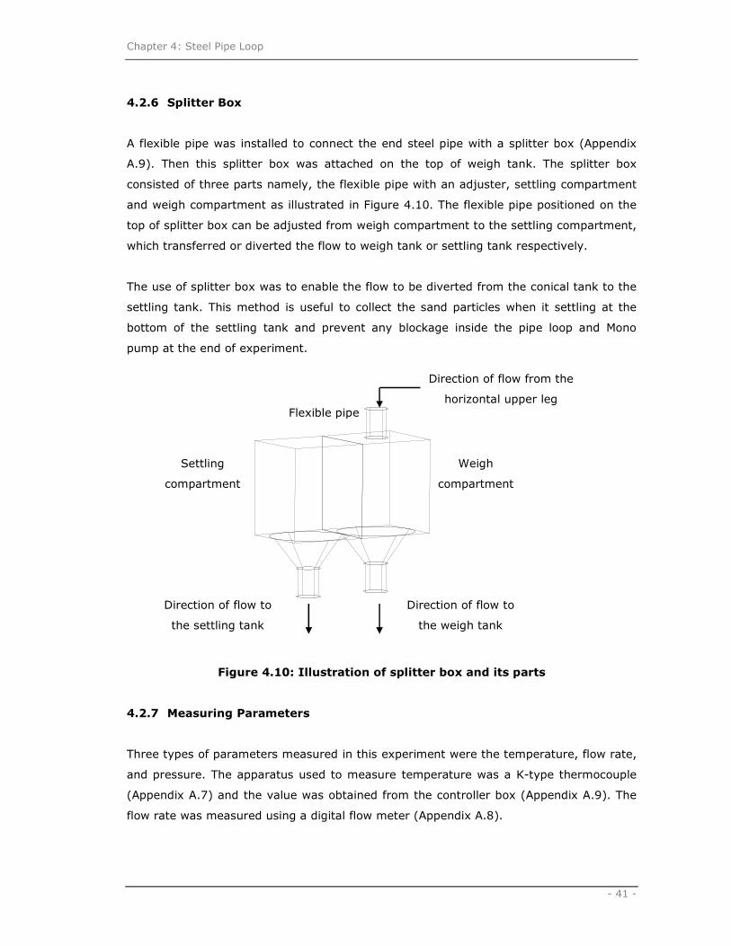
Chapter 4: Steel Pipe Loop
- 41 -
4.2.6 Splitter Box
A flexible pipe was installed to connect the end steel pipe with a splitter box (Appendix
A.9). Then this splitter box was attached on the top of weigh tank. The splitter box
consisted of three parts namely, the flexible pipe with an adjuster, settling compartment
and weigh compartment as illustrated in Figure 4.10. The flexible pipe positioned on the
top of splitter box can be adjusted from weigh compartment to the settling compartment,
which transferred or diverted the flow to weigh tank or settling tank respectively.
The use of splitter box was to enable the flow to be diverted from the conical tank to the
settling tank. This method is useful to collect the sand particles when it settling at the
bottom of the settling tank and prevent any blockage inside the pipe loop and Mono
pump at the end of experiment.
Figure 4.10: Illustration of splitter box and its parts
4.2.7 Measuring Parameters
Three types of parameters measured in this experiment were the temperature, flow rate,
and pressure. The apparatus used to measure temperature was a K-type thermocouple
(Appendix A.7) and the value was obtained from the controller box (Appendix A.9). The
flow rate was measured using a digital flow meter (Appendix A.8).
Settling
compartment
Weigh
compartment
Direction of flow from the
horizontal upper leg
Direction of flow to
the settling tank
Direction of flow to
the weigh tank
Flexible pipe

Chapter 4: Steel Pipe Loop
- 42 -
The objective of this research was to measure the pressure drop when the fluid flows
inside the pipe loop. There were two types of pressure measuring devices had been used
prior before and after the swirl and bend – simple manometer tube and liquid pressure
gauge. Three measuring points were placed as shown in Figure 4.11 to measure the
pressure (1) before the swirl, P1; (2) after the swirl, P2 and; (3) after the bend (and
swirl), P3.
Figure 4.11: The location of pressure measurement – P1, P2 and P3
Initially, the simple manometer tube was used to calculate the pressure when using
water and sand-water slurry fluid based on the elevation of fluids travel along the vertical
tube. The vertical tube was installed vertically up to 9m from the horizontal lower leg
pipe. Due to high concentration and viscosity when using the CMC solutions, the length of
simple manometer tube was not long enough to determine the total length of CMC
solutions travelled along the manometer tube. Therefore, the liquid pressure gauge (up
to 4 bars) was used to replace the simple manometer tube. The simple manometer tube
as shown in Figure 4.12 is a transparent straight tube with 9mm inner diameter and
12mm outer diameter.
P1 P2
P3

Chapter 4: Steel Pipe Loop
- 43 -
Figure 4.12: Simple manometer tube (ID = 9mm and OD = 12mm)
The pressure gauge (also known as Bourdon gauge), shown in Figure 4.13 invented
around 1850, was widely used for measuring the pressure of steam, water, and air up to
100,000 pounds per square inch (psi). The device consists of a flattened circular tube
coiled into a circular arc (Figure 4.14). One end is soldered to a central block and opened
to the fluid, which its pressure to be measured; and the other end is sealed and coupled
to the pointer spindle. When the pressure inside the tube is higher than the outside
pressure, the Bourdon tube will straighten and caused the pointer to turn, which indicate
the pressure reading on a circular scale.
Figure 4.13: A liquid pressure gauge (up to 4 bars)

Chapter 4: Steel Pipe Loop
- 44 -
Figure 4.14: A schematic diagram of Bourdon-tube gauge
(adapted from www.britannica.com)
For pressure measurements, the terms of no swirl, 1 swirl and 2 swirls applied as
follows:
1. No swirl represents the conditions of fluids flow when not preceded with 4-lobe
swirl-inducing pipe flow.
2. 1 swirl represents the conditions of fluids flow when one 4-lobe swirl-inducing pipe
flow (10cm in length) was installed between P1 and P2 as shown in Figure 4.15.
3. 2 swirls represents the conditions of fluids flow when two 4-lobe swirl-inducing
pipes were connected together and installed between P1 and P2 as shown in
Figure 4.16.
Figure 4.15: 1 swirl 4-lobe swirl-inducing pipe flow
Bend
R/D = 4
P2 P1
Direction of
flow

Chapter 4: Steel Pipe Loop
- 45 -
Figure 4.16: 2 swirl 4-lobe swirl-inducing pipes flow connected together
4.3 General Procedures on Steel Pipe Rig
The conical tank was filled with 1.0 m3 of water from the main water. The initial
experiment involved a short circuit flow, which utilised a conical tank and 0.25 m pipe
diameter. The Mono Pump pumped the fluid on short circuit flow at low frequency (5.0 Hz
to 6.0 Hz depends on fluid viscosity) before delivery to a long circuit flow (consisted of a
de-aerator, horizontal lower leg, vertical leg, horizontal upper leg and conical tank) with
a frequency between 8.0 to 35.0 Hz. Water circulated in the pipeline for 10 minutes to
stabilise the flow and ensure tested fluids distributed throughout the flow loop before
taking any readings. The measurements for temperature and pressure were taken in
correspondence to the flow rate. Table 4.1 shows the flow rates and velocities required in
each test.
The above procedures were repeated when using one or two 4-lobe swirl pipe (length =
10cm; internal diameter = 5cm), which was installed at the end of horizontal lower leg,
before the bend as shows in Figure 4.16. Then the same procedure, except for the
application of short circuit, was applied when using sand-water slurry and CMC solution
at different concentrations. To examine sand-water slurries, the conical tank was initially
filled with water depending on the solid concentration requirements. Then sand particles
were added from the top balcony into the conical tank through a weigh tank, as there
was no direct route accessed to conical tank.
P2 P1 Direction of
flow

Chapter 4: Steel Pipe Loop
- 46 -
4.4 Dissolution for Carboxymethyl Cellulose fluid
Before the CMC solutions were mixed constantly at high speed inside a mixer tank, a
biocide solution was added (100 – 130ml) to avoid microbial growth, although it does
give little effect on the rheology of the CMC (Tonkin, 2004). However, it was assumed
(Tonkin, 2004) that the biocide solution will cause give differences to the viscosity and
concentration of CMC. Geldard (2002) claimed that the viscosity of CMC would increase
over the first 24 hours while being hydrated. The CMC solutions appeared as clear fluid
and were tested in the pipe loop for up to five days. When the CMC solution was not in
use, it was stored in the pipe loop.
Table 4.1: Flow rate and velocity for fluid tests
Flow rate Velocity, v (m/s)
Q (m3/hr) Water Slurries (% v/v) CMC (% w/w)
1.4 2.1 2.7 0.5 1.0 1.5
1.414 0.2
2.828 0.4
3.535 0.5
4.242 0.6
5.656 0.8
7.070 1.0
8.483 1.2
9.897 1.4
10.604 1.5
11.311 1.6
12.725 1.8
14.139 2.0
17.674 2.5 2.5
For shutting down procedure, when tested with water alone, the pump was stopped
(frequency was lowered to 10Hz before stopped the pump) and the drain valves opened.
There were two main drain valves each located at the bottom of Mono Pump (Appendix
A.10) and de-aerator (Appendix A.11). In the presence of sand particles (slurries), the
splitter box was switched to pump the solid particles to the settling tank. The water inlet
valve (Appendix A.10) was open to fill the pipe loop with water until some of the sand
particles were pumped to the settling tank. Then the pump was stopped and the slurry
Key:
No
measurement
taken

Chapter 4: Steel Pipe Loop
- 47 -
remains drained through the two drain valves. Inside the settling tank, the sand was
deposited at the bottom, while water was drained off. The shutting down procedure of
the pump when tested with CMC solution was, the water inlet and drained valves were
opened while pumping to clean the pipe loop.
4.5 Summary
This chapter details the components used in the operation of steel pipe rig. Brown Mixer
Tank was used to prepare the requirements of CMC solutions at high volume to be tested
in steel pipe rig and viscosity measurement of CMC. A submersible pump was used to
deliver the CMC solutions inside the mixer tank into the conical tank because the pipe
loop connection between the tanks was not available.
The steel pipe rig used consisted of:
1. Mono pump, which is a progressive cavity type of pumps driven by a motor. The
pumping rate of Mono pump was controlled automatically by adjusting the
frequency of inverter manually.
2. De-aerator to allow any trapped bubbles escape via a tube atmosphere.
3. Conical tank, weigh tank and settling tank at different sizes to fit the volume of
the flow loop and pipeline configuration (Appendix A). The conical tank could
occupy a volume of fluid up to 1.0m3. Settling tank was used to trap sand
particles.
4. Splitter box which transferred or diverted fluids with solid particles from weigh
tank to settling tank respectively.
5. Pressure devices – simple manometer tube or Bourdon gauge (liquid).
6. A pipe loop which consisted of several sections of smooth steel and flexible
perspex pipes, 220mm radii pipe (R/D of 4) and valves.
7. Parameters apparatus – flow rate transducer and digital flow meter, temperature
transducer (K-type).
Three types of fluids were used in the experimental procedures – water, sand-water
slurry and carboxymethyl cellulose (CMC) fluids. The concentrations used for sand-water
slurries were 1.4, 2.1 and 2.7 % v/v. For CMC, the concentrations used were 0.5, 1.0
and 1.5% w/w. The experimental procedure for the steel pipe loop experiments and
viscosity measurements has been described, covering the start up and shut down of the
pipe flow loop for different types of fluids.

Chapter 4: Steel Pipe Loop
- 48 -
Chapter 5
EFFECTS OF 4-LOBE SWIRL INDUCING PIPE
5.1 Introduction
In order to assess the performance of pipeline application, pressure measurements were
assessed. A fluid flow in a pipeline causes pressure changes due to fluctuations in
elevation, friction or flow rates. The Bernoulli equation was applied in this experiment.
This section evaluates the pressure drops of the incompressible flow in straight horizontal
pipe before and after the bend, when preceded with and without swirl-inducing pipes.
In this experiment, the investigation made with slurries was restricted to sand particle
size with a specific gravity of 2.64. The R/D of 4 was used to measure the pressure drop
with and without swirl-inducing pipe effects. The investigation also determined the
similarity of the pressure drop effect obtained from Tonkin (2004) with different
concentration of sand-water slurry.
5.2 Methodology Specifics
Refer to Chapter 4 for viscosity testing of the CMC, fluids preparation and dissolution,
and the operation of the steel pipe loop. For each test fluid and velocity, the pressure
drop was measured at three pressure points, P1, P2 and P3 as illustrated in Figure 5.1:
Figure 5.1: Illustration of pressure locations
P1 P3P2
R/D=4
Directionof flowPressure devices
Swirl pipe

Chapter 4: Steel Pipe Loop
- 49 -
The description of pressure measurement for P1, P2 and P3 are as follows:
1. Pressure point 1 (P1) measured the inlet pressure of fluids when preceded either
by a straight cylindrical or 4-lobe swirl-inducing pipe (lower horizontal leg) before
the bend.
2. Pressure point 2 (P2) measured the outlet pressure of fluids when preceded either
by a straight cylindrical or 4-lobe swirl-inducing pipe (lower horizontal leg) before
the bend.
3. Pressure point 3 (P3) measured the pressure of fluids after preceded with the
effect of bend (R/D = 4) and with or without swirl-inducing pipe.
P2 was installed approximately 40cm from P1 just before the bend (R/D of 4). The swirl-
inducing pipe was installed in between P1 and P2. The pressure drop, ∆P (Pa) against
velocity, v (m/s) was plotted to establish data for comparison at different fluid
conditions. Three conditions of pressure drops, ∆P (Pa) measured included:
1. Pressure drop, ∆P (Pa) on horizontal pipe (lower leg)
2112 PPP −=∆
2. Pressure drop, ∆P (Pa) over the bend (R/D of 4)
3223 PPP −=∆
3. Overall pressure drop across the horizontal pipe and bend (R/D of 4)
31131213 PPPPP −=∆+∆=∆
It was predicted that the ∆P13 ≥ ∆P23 ≥ ∆P12 when the fluids flow velocity (or flow rate)
increased. ∆P12 represents the pressure loss by swirl application.

Chapter 4: Steel Pipe Loop
- 50 -
5.3 Effects of Swirl Inducing Flow over Horizontal Pipe
P1-P2, Water
0
500
1000
1500
2000
0.0 0.5 1.0 1.5 2.0 2.5 3.0
Velocity, v (m/s)
Pre
ssu
re d
rop, ∆P (
Pa)
Figure 5.2: Pressure drop, ∆∆∆∆P12 (Pa) for water over horizontal pipe
Figure 5.2 shows increase in pressure drops, ∆P12 (Pa) when water preceded by swirl-
inducing pipes. As expected, there was no significant pressure drops for ∆P12 (P1-P2)
when the lower leg of horizontal pipe was preceded without swirl inducing pipe. Different
results were discovered when one or two swirl-inducing pipes were installed between
pressure measurements P1 and P2. It was also found that the application of two swirl-
inducing pipes created twice the pressure drops as compared to one swirl-inducing pipe.
The effect of pressure drops, ∆P (Pa) were proportional with velocity, v (m/s) of fluids
flowing inside the pipe. If the velocity, v increase, the pressure drop, ∆P would increase.
At lower velocity of 0.5m/s, the pressure drops for 2 swirls, 1 swirl and no swirl were
almost the similar. However, when the velocity increased to 1.5 m/s, the pressure drops
for 2 swirls, 1 swirl and no swirl were approximately 650Pa, 350Pa and 10Pa
respectively. As the velocity increased up to 2.5 m/s, the 2 swirls and 1 swirl pressure
drops were 1700Pa and 800Pa respectively. The figure shows that the pressure drop
obtained from 2 swirls was almost two times higher than the pressure drop from 1 swirl.
If the water flowing inside the horizontal pipe was not subjected to or preceded with
swirl-inducing pipe, the direction of flows would not be changed. However, when swirl-
inducing pipes were installed, the flow of water changed slightly in its axial horizontal
position. This behaviour can be seen clearly in Figure 5.4 – 5.6 when using slurry.
P1 P3P2
R/D=4
Directionof flowPressure devices
Swirl pipe
2 swirls
1 swirl
No swirl

Chapter 4: Steel Pipe Loop
- 51 -
P1-P2, 1.4 % v/v slurry
0
500
1000
1500
2000
2500
0.0 0.5 1.0 1.5 2.0 2.5 3.0
Velocity, v (m/s)
Pre
ssu
re d
rop, ∆P (
Pa)
(a)
P1-P2, 2.1 % v/v slurry
0
500
1000
1500
2000
2500
0.0 0.5 1.0 1.5 2.0 2.5 3.0Velocity, v (m/s)
Pre
ssure
dro
p, ∆P (
Pa)
(b)
P1-P2, 2.7 % v/v
0
500
1000
1500
2000
2500
0.0 0.5 1.0 1.5 2.0 2.5 3.0
Velocity, v (m/s)
Pre
ssure
dro
p, ∆P (
Pa)
(c)
Figure 5.3: Pressure drop, ∆∆∆∆P12 (Pa) for sand-water slurry at different
concentrations over horizontal pipe (a) 1.4% v/v slurry; (b) 2.1% v/v slurry;
and (c) 2.7% v/v slurry
P1 P3P2
R/D=4
Directionof flowPressure devices
Swirl pipe
2 swirls
1 swirl
No swirl

Chapter 4: Steel Pipe Loop
- 52 -
The effect of 4-lobe swirl-inducing pipe on horizontal pipe was further experimented
using solid-liquid flow (slurry). When using slurries, similar curves were found as shown
in Figure 5.3. The pressure drops, ∆P12 for sand-water slurries on horizontal pipe
increased with slurries concentrations. The swirling flow application also increased the
∆P12 for slurries (depending on a length of swirl flow induced) compared to no swirl-
inducing pipe application on the horizontal pipe.
At lower velocity of 0.5 m/s, the pressure drops at 1.4% v/v slurry concentration for 2
swirls, 1 swirl and no swirl were approximately 500Pa, 200Pa and 20Pa respectively. The
pressure drop changes were not significant at lower velocity. However, at 1.5 m/s, the
pressure drops at 1.4% v/v, 2.1% v/v and 2.7% v/v slurry concentrations for 2 swirls
were approximately 1650 - 1700Pa. The pressure drops for 1 swirl were approximately
870Pa, 1150Pa and 1400Pa. The pressure drops for no swirl application at 1.4% v/v,
2.1% v/v and 2.7% v/v slurry concentrations were approximately 140 – 150Pa.
It was predicted that the pressure drops for no swirl-inducing pipe performed were not
significant even though the slurries flowed at different concentrations on the horizontal
pipe. It was because there were no changes on flow direction along horizontal pipe.
However, the application of 1 and 2 swirl-inducing pipes increased the pressure drops as
the velocity of the slurry increased. 1 swirl gave distinctive values of pressure drops
compared to 2 swirls application.
Figures 5.4 – 5.6 shows the visualisation of flow behaviour for 1.4% v/v sand particles
slurries when travelled at 1.5m/s. As shown in figure 5.4, the sand particles behaved as
a flow with moving bed. After preceded with swirl-inducing pipe flow, the sand particles
tend to distribute evenly as shown in Figure 5.5. From this visualisation, the swirl-
inducing pipe worked as a lifter (as shown in Figure 5.6) for solid-liquid mixture. This
increased the sand particles homogeneity and subsequently reduced the solid particles
friction across the pipe wall.
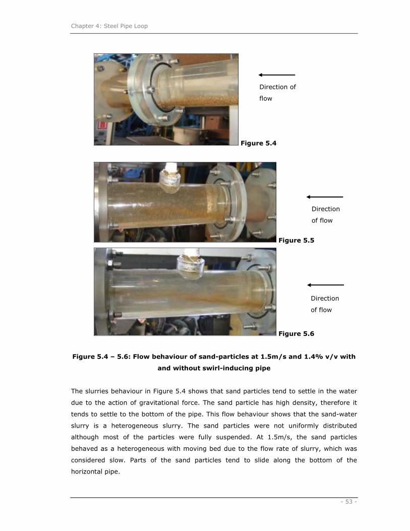
Chapter 4: Steel Pipe Loop
- 53 -
Figure 5.4
Figure 5.5
Figure 5.6
Figure 5.4 – 5.6: Flow behaviour of sand-particles at 1.5m/s and 1.4% v/v with
and without swirl-inducing pipe
The slurries behaviour in Figure 5.4 shows that sand particles tend to settle in the water
due to the action of gravitational force. The sand particle has high density, therefore it
tends to settle to the bottom of the pipe. This flow behaviour shows that the sand-water
slurry is a heterogeneous slurry. The sand particles were not uniformly distributed
although most of the particles were fully suspended. At 1.5m/s, the sand particles
behaved as a heterogeneous with moving bed due to the flow rate of slurry, which was
considered slow. Parts of the sand particles tend to slide along the bottom of the
horizontal pipe.
Direction of
flow
Direction
of flow
Direction
of flow

Chapter 4: Steel Pipe Loop
- 54 -
Tonkin (2004) discovered that fine (118µm) or medium (500-1000µm) sand particle
exhibited the same characteristics as slurry flow and tends to settle. In a horizontal pipe,
the sand particles settled at the bottom of the pipe cross-section. This phenomenon
formed heterogeneous flow behaviour. When the settling slurry proceeded from
horizontal to vertical pipe, the particles behaved as homogeneous flow and distributed
well in the pipe-cross section. This similar effect can be visualised when the sand-water
mixtures were preceded with swirl-inducing pipe as shown in Figures 5.5 and 5.6.
The experimental data showed that there was a lift force produced by flow from the bend
effect to repel the sand particles from the wall when travelled across vertical pipe. This
phenomenon contributed to a pressure drop. When swirl-inducing pipe flow was applied,
the same characteristics was observed, where coarse particles were homogeneously
distributed.
It was predicted that the sand particles travelled at higher velocity compared to without
swirling flow as shown in Figure 5.6. The swirl-inducing pipe created a lift force (or acted
as a lifter) between the sand particle and carrier fluid flow across the swirl-inducing pipe.
This behaviour was responsible for the reduction of pressure drop over the bend (∆P23)
and low secondary flow generation as shown in Figure 5.9.
As mentioned in Chapter 3 (Test Materials), the CMC fluid exhibited non-Newtonian
characteristics (shear thinning, power-law). When experimented at nominal velocities
ranging from 0.2 to 2.5 m/s, the CMC fluids travelled within a laminar regime (Appendix
B; Table B.4) compared to water and sand-water slurries which travelled in a turbulent
regime. The pressure drops, ∆P12 (Pa) for CMC exhibited similar curves with water (figure
5.2) and slurries (figure 5.3) as shown in Figure 5.6. At a higher concentration (1.5%
w/w) the ∆P12 for CMC was not significant when preceded either by one or two
applications of swirl-inducing pipe (Appendix C.14). The application of one 4-lobe swirl-
inducing pipe and straight cylinder pipe showed no significant pressure drop behaviour
for CMC at concentrations 0.5 and 1.0 % w/w.

Chapter 4: Steel Pipe Loop
- 55 -
P1-P2, 0.5% w/w CMC
0
1000
2000
3000
4000
5000
6000
7000
8000
0.0 0.5 1.0 1.5 2.0 2.5 3.0Velocity, v (m/s)
Pre
ssure
dro
p, ∆P (
Pa)
(a)
P1-P2, 1.0% w/w CMC
0
1000
2000
3000
4000
5000
6000
7000
8000
0.0 0.5 1.0 1.5 2.0 2.5 3.0
Velocity, v (m/s)
Pre
ssure
dro
p, ∆P (
Pa)
(b)
Figure 5.7: Pressure drop, ∆∆∆∆P12 (Pa) for carboxymethyl cellulose at different
concentration over horizontal pipe (a) 0.5% w/w CMC; and (b) 1.0% w/w CMC
P1 P3P2
R/D=4
Directionof flowPressure devices
Swirl pipe
2 swirls
1 swirl
No swirl

Chapter 4: Steel Pipe Loop
- 56 -
The effect of 4-lobe swirl inducing pipe was further investigated using carboxymethyl
cellulose (CMC) as a non-Newtonian fluid. As shown in Figure 5.7, the pressure drops for
both concentrations at 0.5 and 1.0% w/w CMC were increased with increasing velocity, v
(m/s). The 2 swirls gave higher pressure drops compared to 1 swirl and no swirl
applications along the horizontal pipe. The 0.5% w/w CMC was experimented up to
2.0m/s and the pressure drops were calculated and measured using a simple manometer
tube (Figure 4.15). The pressure drops, ∆P12 for CMC at 1.0 and 1.5% w/w were
determined using Bourdon gauge (a liquid pressure gauge).
The pressure drops, ∆P12 at concentration of 0.5% w/w CMC and 0.5 m/s velocity for 2
swirls, 1 swirl and no swirl were approximately 430Pa, 270Pa and 130Pa respectively as
shown in figure 5.7(a). When the velocity increased up to 2.0m/s, the pressure drops for
2 swirls, 1 swirl and no swirl application were approximately 2200Pa, 1000Pa and 260Pa
respectively. At approximately 18°C, CMC had a high apparent viscosity of 0.15 Ns/m2.
Due to this characteristic, when flow rates or velocity were increased, the pressure drops
along horizontal pipe increased up to 500% depending on the application of swirl-
inducing pipes.
Figure 5.7(b) shows the effect of swirl-inducing flow for the CMC at 1.0 w/w and 0.5m/s
velocity with pressure drops, ∆P12 of approximately 1900Pa, 1400Pa and 700Pa for 2
swirls, 1 swirl and no swirl respectively. At velocity of 2.0m/s, the pressure drops were
approximately 4700Pa, 3400Pa and 2600Pa respectively. The CMC fluid which travelled
at 0.5m/s had 670Re. The apparent viscosity for CMC at 1.0% w/w and 18°C was 0.712
Ns/m2, which when pumped at 2.0m/s had 140Re. The CMC fluids at these two
concentrations were flowing under a laminar regime (Appendix B: Table B.4). Its high
viscosity and low Reynolds number contributed to an increase in pressure drops when the
CMC fluids were preceded with a swirl-induced flow.

Chapter 4: Steel Pipe Loop
- 57 -
5.4 Effects of Swirl Inducing Flow over the Bend (R/D of 4)
In pipework, valves, fittings, or bends can cause impact to the pressure drop and the
distribution of flow (Azzi, Friedel and Belaadi; 2000). The following results show the
changes which occurred when swirl-inducing pipe was used in straight horizontal pipeline.
P2-P3, Water
8500
9000
9500
10000
0.0 0.5 1.0 1.5 2.0 2.5 3.0
Velocity, v (m/s)
Pre
ssu
re d
rop, ∆P (
Pa)
Figure 5.8: Pressure drop, ∆∆∆∆P23 (Pa) for water over the bend (R/D = 4)
Figure 5.8 shows a graph of pressure drop, ∆P23 (Pa) against velocity, v (m/s) ranging at
0.5 – 2.5m/s. The pressure drops at 0.5m/s were not significant (approximately 9000Pa)
among 2 swirls, 1 swirl and no swirl application. As the velocity of water increased, the
pressure drops for no swirl application were higher compared to swirl-induced pipe flow.
At 1.5m/s, the pressure drops for 2 swirls, 1 swirl and no swirl were approximately
9200Pa, 9200Pa and 9300Pa respectively and at 2.5m/s, were approximately 9350Pa,
9400Pa and 9600Pa. The overall pressure drops over the bend when the velocity
increased for water was approximately 50 – 300Pa higher compared to swirl-induced
flow.
P1 P3P2
R/D=4
Directionof flowPressure devices
Swirl pipe
2 swirls
1 swirl
No swirl

Chapter 4: Steel Pipe Loop
- 58 -
P2-P3, 1.4 % v/v
8000
9000
10000
11000
12000
0.0 0.5 1.0 1.5 2.0 2.5 3.0
Velocity, v (m/s)
Pre
ssure
dro
p, ∆P (
Pa)
(a)
P2-P3, 2.1 % v/v
8000
9000
10000
11000
12000
0.0 0.5 1.0 1.5 2.0 2.5 3.0
Velocity, v (m/s)
Pre
ssure
dro
p, ∆P (
Pa)
(b)
P2-P3, 2.7 % v/v
8000
9000
10000
11000
12000
0.0 0.5 1.0 1.5 2.0 2.5 3.0
Velocity, v (m/s)
Pre
ssure
dro
p, ∆P (
Pa)
(c)
Figure 5.9: Pressure drop, ∆∆∆∆P23 (Pa) for sand-water slurry at different
concentrations over the bend with and without swirl inducing pipe
P1 P3P2
R/D=4
Directionof flowPressure devices
Swirl pipe
2 swirls
1 swirl
No swirl

Chapter 4: Steel Pipe Loop
- 59 -
Figure 5.9 shows that the pressure drop of 1.4, 2.1 and 2.7% v/v slurry without swirl-
inducing pipe increases against velocity. The ∆P23 (Pa) over the bend was reduced after
the slurries passed through the swirl inducing pipe flow. Pressure drop in the bend was
reduced due to the reacceleration of fluids during transit. It is assumed that the pressure
dropped due to bend effects, which consisted of wall friction and momentum exchange
between the liquid and pipe wall. Secondary flow generation and the bend arrangement
in either upstream or downstream also affected the pressure drop.
The 10cm length of the 4-lobe swirl pipe (1 swirl pipe) showed a lower pressure drop
than the 20cm length of 4-lobe swirl pipe (2 swirl pipes). This was true for an
approximate velocity of 1.5 m/s onwards. Both swirl applications showed lower pressure
drops compared to not having a swirl-inducing pipe. At velocity of 0.5m/s, the ∆P23 for 2
swirls, 1 swirl and no swirl were approximately 9200 Pa, 9000 Pa and 10,000 Pa
respectively. The ∆P23 without swirl-inducing pipe showed increase in pressure drop
compared to 2 swirls and 1 swirl approximately 9 and 11%. For 2.1 and 2.7% w/w
slurry, the ∆P23 without swirl-inducing pipe increased approximately 9-11% and 6-%
respectively.
Normally, when fluid travels over a bend, there will be a significant pressure drop created
by the existence of secondary generation flows. This phenomenon (secondary generation
flows) is produced by a combination of centrifugal force, which depended on the
movement of a fluid directed from the momentaneous centre of curvature to the outer
wall, and the effect from the boundary layer at the wall of the bend (Azzi et al., 2000).
The swirl-induce pipe tend to create a swirling flow, which caused less centrifugal forces
and shear stress on the boundary layer over a bend. The mechanical behaviour of the
swirl inducing pipe as a lifter (creating homogeneous distribution over a pipe cross
section) also contributed to a reduction of pressure drop over the bend.

Chapter 4: Steel Pipe Loop
- 60 -
P2-P3, 0.5% w/w CMC
2000
4000
6000
8000
10000
12000
0.0 0.5 1.0 1.5 2.0 2.5 3.0
Velocity, v (m/s)
Pre
ssure
dro
p, ∆P (
Pa)
(a)
P2-P3, 1.0% w/w CMC
2000
4000
6000
8000
10000
12000
0.0 0.5 1.0 1.5 2.0 2.5 3.0
Velocity, v (m/s)
Pre
ssure
dro
p, ∆P (
Pa)
(b)
Figure 5.10: Pressure drop, ∆∆∆∆P23 (Pa) for CMC at (a) 0.5% w/w CMC, and (b)
1.0% w/w CMC, concentrations over the bend
When 0.5% w/w CMC was preceded without swirl-induced flow, it had a similar trend of
graph with water and slurries. The pressure drops for no swirl application were higher
than swirl-inducing flow as shown in figure 5.10 (a). At 0.5m/s, the pressure drops for 2
swirls, 1 swirl and no swirl were approximately 5500Pa, 5470Pa and 5600Pa respectively.
When the velocity increased up to 2.0m/s, the pressure drops were approximately
10000Pa, 9700Pa and 10200Pa respectively.
When the concentration of CMC was increased to 1.0% w/w, the CMC fluids travelled
under a laminar regime (140Re). Due to this flow behaviour, the pressure drops obtained
in Figure 5.10(b) at 0.5m/s for 2 swirls, 1 swirl and no swirl were approximately 3600Pa,
3100Pa and 4300Pa respectively. At 2.0m/s, the pressure drops obtained were
approximately 6200Pa, 4500Pa and 5300Pa respectively.
P1 P3P2
R/D=4
Direction
of flowPressure devices
Swirl pipe
2 swirls
1 swirl
No swirl

Chapter 4: Steel Pipe Loop
- 61 -
The pressure drops for a non-Newtonian fluid at different concentrations and viscosity
produced different trends of curves. The CMC fluids which proceeded without swirl-
inducing flow had higher pressure drops compared to swirl-inducing pipe flow as shown
in Figure 5.10(a). However, when the concentration of non-Newtonian fluid was
increased and had lower Reynolds number, the pressure drops for swirl-induced pipe
would be higher compared to flow without swirl-inducing pipe. The same results were
obtained for CMC fluid 1.5% w/w (Appendix C:17). At 2.0m/s, the pressure drops for 2
swirls, 1 swirl and no swirl were approximately 12400Pa, 11200Pa and 8300Pa
respectively.
5.5 Effects of Swirl Inducing Pipe Across Pipe
Based on theoretical assumption (Clayton, 2006) that under the same operating
conditions (such as velocity, pipe diameter and length, etc.), increases in the slurries
concentrations will increase the overall pressure drop (∆P13) across the horizontal pipe
and bend with and without swirl-inducing pipe. To test this hypothesis, measurements
were made for various flow velocities ranging 0.5 – 2.5 m/s.
P1-P3, Water
8500
9500
10500
11500
12500
13500
14500
0.0 0.5 1.0 1.5 2.0 2.5 3.0
Velocity, v (m/s)
Pre
ssu
re d
rop, ∆P (
Pa)
Figure 5.11: Pressure drop, ∆∆∆∆P13 (Pa) for water across pipe
Figure 5.11 shows that the pressure drop for water increased with velocity, v (m/s) after
preceded with the 4-lobe swirl-inducing pipe. At lowest operating velocity of 0.5m/s, the
pressure drops for both conditions, with and without swirl-inducing pipe were not
significant. At a high velocity of 2.5 m/s, the pressure drop, ∆P12 for 2 swirls and no
swirls were 11200 Pa and 9700 Pa respectively. The 2 swirls caused higher pressure
P1 P3P2
R/D=4
Directionof flowPressure devices
Swirl pipe
2 swirls
1 swirl
No swirl
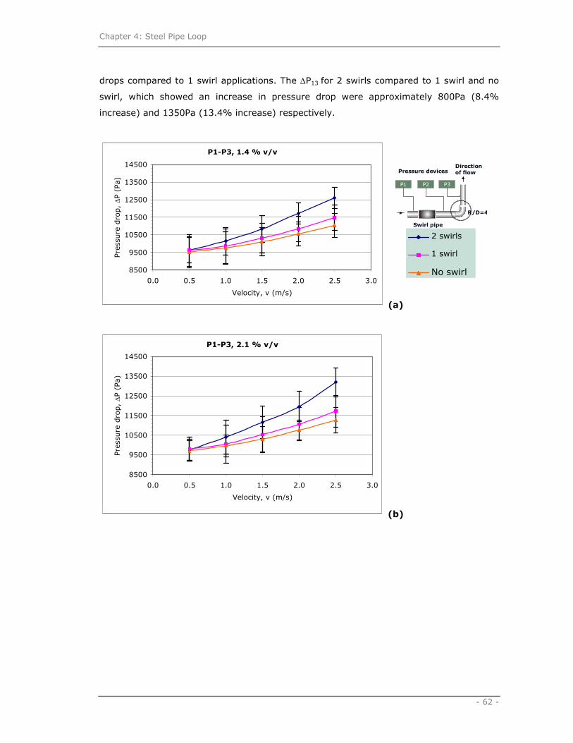
Chapter 4: Steel Pipe Loop
- 62 -
drops compared to 1 swirl applications. The ∆P13 for 2 swirls compared to 1 swirl and no
swirl, which showed an increase in pressure drop were approximately 800Pa (8.4%
increase) and 1350Pa (13.4% increase) respectively.
P1-P3, 1.4 % v/v
8500
9500
10500
11500
12500
13500
14500
0.0 0.5 1.0 1.5 2.0 2.5 3.0
Velocity, v (m/s)
Pre
ssure
dro
p, ∆P (
Pa)
(a)
P1-P3, 2.1 % v/v
8500
9500
10500
11500
12500
13500
14500
0.0 0.5 1.0 1.5 2.0 2.5 3.0
Velocity, v (m/s)
Pre
ssure
dro
p, ∆P (
Pa)
(b)
P1 P3P2
R/D=4
Directionof flowPressure devices
Swirl pipe
2 swirls
1 swirl
No swirl

Chapter 4: Steel Pipe Loop
- 63 -
P1-P3, 2.7 % v/v
8500
9500
10500
11500
12500
13500
14500
0.0 0.5 1.0 1.5 2.0 2.5 3.0
Velocity, v (m/s)
Pre
ssu
re d
rop
, ∆P (
Pa)
(c)
Figure 5.12: Pressure drop, ∆∆∆∆P13 (Pa) for slurries at different concentrations
across pipe (a) 1.4% v/v; (b) 2.1% v/v; and (c) 2.7% v/v
The effects of swirl-inducing flow on pressure drop for sand-water slurries at different
concentrations in Figure 5.12, suggested that the application of swirl pipe increased the
pressure drop over a standard pipe. When sand-water slurries were induced with swirl
flow, the settling of sand particles decreased as velocity increased. At velocity of 2.5 m/s,
the total pressure drops for 2.7% v/v slurry concentration across pipe for no swirl, 1 swirl
and 2 swirls were approximately 11,500 Pa, 12200 Pa and 13,300 Pa respectively. The
pressure drop, ∆P (Pa) increased approximately 16% when using 2 swirls and this varied
with the concentration of slurries.
Figure 5.13: Pressure drop, ∆∆∆∆P (Pa) over horizontal pipes for coarse sand
slurries (2000µµµµm) (taken from Tonkin, 2004)
P1 P3P2
R/D=4
Directionof flowPressure devices
Swirl pipe
2 swirls
1 swirl
No swirl
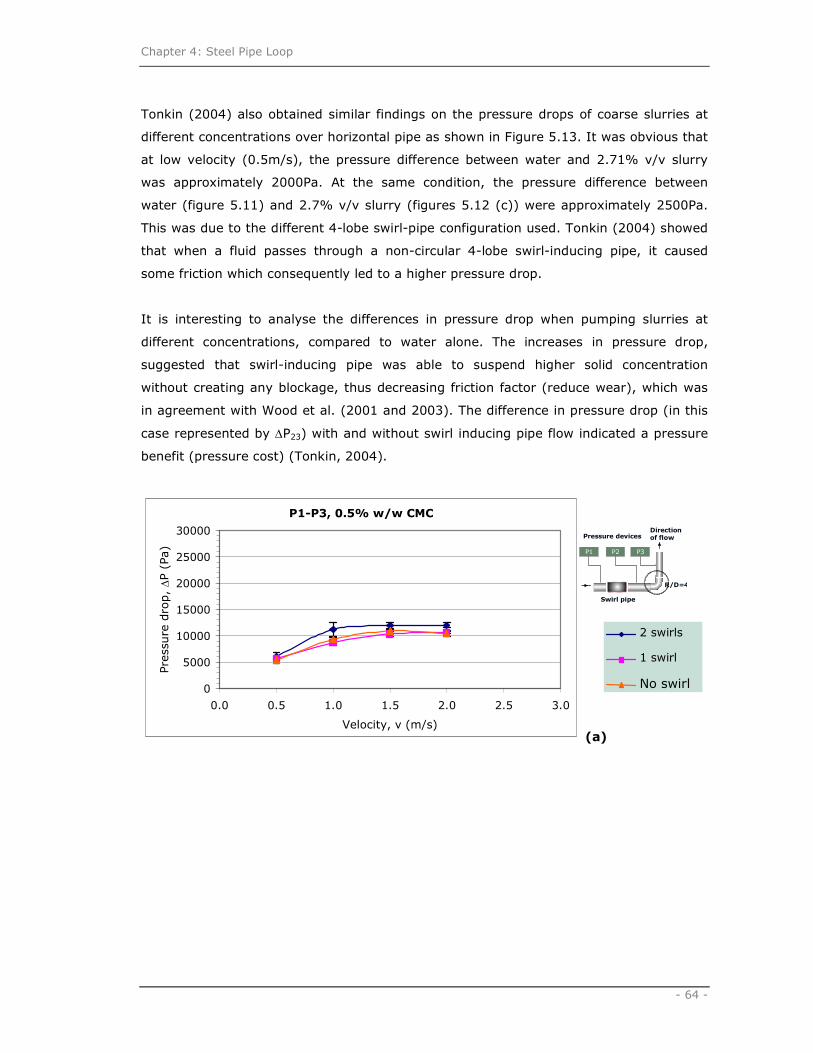
Chapter 4: Steel Pipe Loop
- 64 -
Tonkin (2004) also obtained similar findings on the pressure drops of coarse slurries at
different concentrations over horizontal pipe as shown in Figure 5.13. It was obvious that
at low velocity (0.5m/s), the pressure difference between water and 2.71% v/v slurry
was approximately 2000Pa. At the same condition, the pressure difference between
water (figure 5.11) and 2.7% v/v slurry (figures 5.12 (c)) were approximately 2500Pa.
This was due to the different 4-lobe swirl-pipe configuration used. Tonkin (2004) showed
that when a fluid passes through a non-circular 4-lobe swirl-inducing pipe, it caused
some friction which consequently led to a higher pressure drop.
It is interesting to analyse the differences in pressure drop when pumping slurries at
different concentrations, compared to water alone. The increases in pressure drop,
suggested that swirl-inducing pipe was able to suspend higher solid concentration
without creating any blockage, thus decreasing friction factor (reduce wear), which was
in agreement with Wood et al. (2001 and 2003). The difference in pressure drop (in this
case represented by ∆P23) with and without swirl inducing pipe flow indicated a pressure
benefit (pressure cost) (Tonkin, 2004).
P1-P3, 0.5% w/w CMC
0
5000
10000
15000
20000
25000
30000
0.0 0.5 1.0 1.5 2.0 2.5 3.0
Velocity, v (m/s)
Pre
ssu
re d
rop, ∆P (
Pa)
(a)
P1 P3P2
R/D=4
Directionof flowPressure devices
Swirl pipe
2 swirls
1 swirl
No swirl

Chapter 4: Steel Pipe Loop
- 65 -
P1-P3, 1.0% w/w CMC
0
5000
10000
15000
20000
25000
30000
0.0 0.5 1.0 1.5 2.0 2.5 3.0
Velocity, v (m/s)
Pre
ssure
dro
p, ∆P (
Pa)
(b)
P1-P3, 1.5% w/w CMC
0
5000
10000
15000
20000
25000
30000
0.0 0.5 1.0 1.5 2.0 2.5 3.0
Velocity, v (m/s)
Pre
ssure
dro
p, ∆P (
Pa)
(c)
Figure 5.14: Pressure drop, ∆∆∆∆P13 (Pa) against velocity, v (m/s) CMC at different
concentrations (a) 0.5% w/w; (b) 1.0% w/w; and (c) 1.5%% w/w
Initially, the pressure drop measurements were performed using a simple manometer
tube. Due to high concentrations and viscosities of CMC at 1.0 and 1.5 % w/w, the
flexible pipes connected to and from de-aerator were disjointed. Therefore, the pressure
measurements were measured using a Bourdon gauge. The accuracy of using Bourdon
gauge was ± 0.05 bars (5000 Pa), suggesting that a better pressure device was required
to estimate the pressure changes when using non-Newtonian fluids at higher
concentrations and viscosity.
P1 P3P2
R/D=4
Directionof flowPressure devices
Swirl pipe
2 swirls
1 swirl
No swirl
Chapter 4: Steel Pipe Loop
- 66 -
Figure 5.14 shows the overall pressure drop, ∆P13 (Pa) ( )31 PP − for CMC at different
concentrations when preceded with and without swirl inducing pipe flow. The result
shows that the pressure drops, ∆P13 (Pa) increased with increasing concentrations. In
Figure 5.14 (a), the ∆P13 (Pa) proceeded with two 4-lobe swirl-inducing pipes increased
at velocities between 0.5 and 1.0 m/s. However, no significant changes were obtained for
∆P13 when performed at velocities between 1.5 and 2.0 m/s.
Figure 5.14 (b) and (c) shows that the ∆P13 (Pa) obtained were small between no swirl
and with swirl applications. The characteristics at ∆P13 between one and two 4-lobe swirl-
inducing pipes were not significant for CMC at 1.5% w/w. This was because at 1.0 and
1.5 % w/w, the CMC fluids travelled at laminar regimes (Recmc < 2000). Therefore, the
comparison of pressure drops between the applications of 1 swirl and 2 swirls was not
able to be determined. In this case, further investigation should be performed at higher
velocity profiles using better pressure device to analyse the effect for 1 swirl and 2 swirls
with non-Newtonian fluids.

Chapter 4: Steel Pipe Loop
- 67 -
5.6 Summary
The pressure measurements were assessed to evaluate the pressure drops of the
incompressible flow of water, slurries and CMC in straight horizontal pipe before and after
the bend, when preceded with and without swirl-inducing pipes. The sand particle size
used in slurry had a specific gravity of 2.64.
The pressure points for P1, P2 and P3 were located before and after the swirl-induced
pipe, and after the bend (R/D=4), respectively. Three pressure drops, ∆P (Pa) were
calculated as follows:
1. ∆P12 for the effect of 4-lobe swirl-induced pipe on horizontal pipe (lower leg).
2112 PPP −=∆
2. ∆P23 for the effect of 4-lobe swirl-induced pipe over the bend (R/D of 4) to indicate
the pressure loss due to swirl-inducing flow.
3223 PPP −=∆
3. ∆P13 for the effect obtained in ∆P12 and ∆P23
31131213 PPPPP −=∆+∆=∆
The graphs of pressure drop, ∆P (Pa) against velocity, v (m/s) were plotted to establish
data for comparison at different fluid conditions.
The pressure drops, ∆P12 (Pa) for water preceded by swirl-inducing pipes were increased
compared to application with no swirl. Furthermore, the application of 2 swirls gave
higher pressure drops when compared to 1 swirl pipe.
The pressure drops, ∆P12 for slurries on horizontal pipe increased with slurries
concentrations but no significant changes were obtained at lower velocity of 0.5m/s. The
application of 1 and 2 swirl-inducing pipes increased the pressure drops as the velocity of
the slurry increase. 1 swirl gave distinctive values of pressure drops when compared to 2
swirls application.
Along the horizontal pipe, the sand particles were observed to be settled at the bottom of
pipe due to gravitational force. However, when the sand particles were preceded with
swirl-induced pipe, the sand particles behaved homogeneously and distributed well in a
pipe-cross section.

Chapter 4: Steel Pipe Loop
- 68 -
The sand particles tend to distribute evenly due to swirl-inducing flow, which lifted the
solid-liquid mixture and changed the flow direction in its axial line along the horizontal
pipe. This increased the sand particles homogeneity and decreased the pressure drops,
∆P23.
The CMC fluid exhibited non-Newtonian characteristics and travelled within a laminar
regime when experimented at nominal velocities ranging from 0.2 to 2.5 m/s. The
pressure drops, ∆P12 (Pa) for CMC gave higher pressure drops compared to water and
slurries because of high apparent viscosity. However, the ∆P12 for 1.5% w/w CMC was
not significant when preceded by swirl-inducing pipe.
The pressure drops, ∆P23 (Pa) over the bend for water and slurries were reduced after
proceeded by swirl-inducing pipe flow due to the reacceleration of fluids when travelled
over the bend. Secondary generation flows also affected the pressure drop over the
bend. However, the pressure drops, ∆P23 (Pa) for CMC fluids produced different results as
the swirl-induced pipe gave higher pressure drops compared to application with no swirl.
The ∆P23 (Pa) for CMC exhibited irregular curves. Further investigation is required.
The overall pressure drops, ∆P13 (Pa) for water, slurries and CMC were increased due to
the swirl-inducing pipe. The pressure drops, ∆P (Pa) across a pipe increased and was
summarised as follows:
a. ∆P (high concentration) ≥ ∆P (low concentration)
b. ∆P13 ≥ ∆P12 ≥ ∆P23
c. Increased the flow rates, increasing the ∆P
The application of two swirl pipes showed further increase in ∆P compared to using one
4-lobe swirl-inducing pipe, which depended on the velocity and types of fluids tested:
∆P (2 swirls) ≥ ∆P (1 swirl) ≥ ∆P (no swirl)

Chapter 6: Conclusions and Recommendations
- 69 -
Chapter 6
CONCLUSIONS AND RECOMMENDATIONS
The effect of 4-lobe swirl-inducing pipe on pressure drop, ∆P was investigated at different
concentrations and flow rates.
6.1 Effect of 4-Lobe Swirl-Inducing Pipe on Settling Slurries
1. The 4-lobe swirl pipe increased the pressure drop, ∆P on settling slurries across a
pipe but reduced the ∆P over the bend.
2. The sand-water slurry exhibited homogeneous flow when preceded with 4-lobe
swirl pipe. Swirling flow increased the sand particles homogeneity and
subsequently reduced the solid particles friction across the pipe wall.
3. At high velocity, the sand particles were evenly distributed when proceeded with
swirl-inducing pipe. This showed that the application of swirl-inducing flow was
most effective even at higher slurry concentrations.
6.2 Effect of 4-lobe Swirl-Inducing Pipe on Non-Newtonian Fluid
Carboxymethyl cellulose (CMC) exhibited power-law or shear thinning fluid. At nominal
velocity between 0.2 and 2.5 m/s, CMC flowed within a laminar regime.
The pressure drops, ∆P increased when 4-lobe swirl pipe was used compared to without
swirl-inducing pipe.
The application of using either one or two 4-lobe swirl pipes on ∆P showed almost similar
results. Application at higher velocities needs to be performed and better pressure
devices should be used.
The pressure drop over a bend for CMC was higher compared to sand-water slurries and
water. The swirl-inducing pipe had no decreasing effect the pressure drops over a bend
compared to slurries and water.
Chapter 6: Conclusions and Recommendations
- 70 -
6.3 Contribution of Thesis
1. Swirling flow application reduced the pressure drop, ∆P over the bend but
increased the ∆P across a pipe. However, these results do not fully apply to CMC
as it travelled at laminar regime and had higher viscosity.
2. Swirling flow increased the sand particles distribution in a pipe-cross section.
3. The application of two swirl pipes showed increased in ∆P compared to one 4-lobe
swirl-inducing pipe or without swirl-inducing pipe.
4. The effect of 4-lobe swirl-inducing pipe on ∆P over the bend is reduced. The swirl-
induced pipe tend to create a swirling flow or orientation of the fluid, which
caused less centrifugal forces and shear stress on the boundary layer over the
bend and led to low secondary generation.
6.4 Recommendations
The experimental data was performed with a pipe diameter of 0.05m under different
conditions. Results indicate that the use of swirl-inducing pipe increased the pressure
drop across the horizontal pipe but reduced the pressure drop over the bend (R/D of 4).
It is recommended that the swirl-inducing pipe of 4-lobe should be performed at smaller
pipe diameter (1cm or less) and thickness as well as on 90o bend.
The modelling on 4-lobe swirl-inducing pipe should be carried out intensively to ensure it
gives a better performance on any types of fluid especially when the swirl-inducing pipe
is applied before a bend.
The application of 180o bend is very common in the pipeline system, condenser,
evaporator etc. It is recommended to investigate the swirl-inducing flow behaviours and
effects when using vertical or horizontal 180o bends.

References
- 71 -
REFERENCES
Agarwal, N., and Chhabra, R.P., (2007) ‘Settling velocity of cubes in Newtonian and
power law liquids’, Powder Technology, Vol. 178, pp17-21.
Akpinar E.K., and Bicer, Y., (2005) ‘Investigation of heat transfer and exergy loss in a
concentric double pipe exchanger equipped with swirl generators’, International Journal
of Thermal Sciences, Vol. 44, Issue 6, pp598-607
Azzi, A., Friedel, L., and Belaadi, S., (2000) ‘Two-phase gas/liquid flow pressure loss in
bends’, Forschung im Ingenieurwesen, Vol. 65, pp309-318.
Azzopardi, B.J., (2006), Personal Communication
Azzopardi, B.J., (2007), Personal Communication
Ayukawa, K. (1969) ‘Pressure Drop in the Hydraulic Conveyance of Solids Materials
Through a Bend in a Vertical Plane’, Bull. JSME Vol. 12, No.54, pp1388-1396.
Brookfield Engineering Laboratories, Inc. Middleboro, MA, USA, http://www.can-
am.net/suppliers/brookfield/dial_new.pdf (last accessed on 3rd February 2007)
Brown, N.I, & Heywood, N.I., (1991) Slurry Handling: Design of Solid-Liquid Systems.
Elsevier Science Publishers, London.
Cenna, A.A., Page, N.W., Williams, K.C., and Jones, M.G., (2007) ‘Wear mechanisms in
dense phase pneumatic conveying of alumina’, Wear.
Chanchala Ariyaratne (2005) Design and Optimisation of Swirl Pipes and Transition
Geometries for Slurry Transport. PhD Thesis 2005. School of Chemical, Environmental
and Mining Engineering, University of Nottingham, United Kingdom.
Charles, M.E., and Charles, R.A., (1971) ‘The use of heavy media in the pipeline
transport of particulate solids’, In Advances in Solid-Liquid Flow in Pipes and Its
Applications, Ed. I. Zandi, Pergamon Press, Oxford, pp187-197.
References
- 72 -
Chu, K.C., and A.B. Yu, A.B., (2007) ‘Numerical simulation of complex particle–fluid flows
Powder Technology.
Cilliers, J.J., Xie, W., Neethling, S.J., Randall, E.W., and Wilkinson, A.J., (2001),
‘Electrical resistance tomography using a bi-directional current pulse technique’, Meas.
Science Technology, Vol. 12, pp997-1001.
Clayton T. Crowe (2006) Multiphase Flow Handbook.
Daniel D. Joseph (2005) Potential flow of viscous fluids: Historical notes; Department of
Aerospace Engineering and Mechanics; University of Minnesota.
Darby, R., (2001) Chemical Engineering Fluid Mechanics: Second Edition, Revised and
Expanded, Texas A & M University, College Station, New York.
Dehbi, A., (2007) ‘A CFD model for particle dispersion in turbulent boundary layer flows’,
Nuclear Engineering and Design.
Delgado, M.A., Franco, J.M., Partal, P., and Gallegos, C., (2005) ‘Experimental study of
grease flow in pipelines: wall slip and air entrainment effects’, Chemical Engineering and
Processing, Vol. 44, Issue 7, pp805-817
Doron, P., and Barnea, D., (1995) ‘Pressure drop and limit deposit velocity for solid-liquid
flow in pipes’, Pergamon, Vol. 50, No. 10, pp1595-1640.
Donald S. Miller; Internal flow: A guide to losses in pipe and duct systems
Fangary, Y.S., Abdel Ghani, A.S., El Haggar, S.M., and Williams, R.A., (1997), ‘The effect
of fine particles on slurry transport processes’, Minerals Engineering, Vol. 10, No.4,
pp427 – 439.
Ganeshalingam, J., (2002) Swirl-Induction for Improved Solid-Liquid Flow in Pipes. PhD
Thesis, 2002. School of Chemical, Environmental and Mining Engineering, University of
Nottingham, United Kingdom.

References
- 73 -
Geldard, R.J.J., Jones, T.F., Miles, N.J., and Rhodes, N.J., (2002) Selection of a suitable
non-Newtonian fluid for swirling pipe flow tests. BHR Group, Hydrotransport, Vol. 15,
pp287–298.
Geldard, R.J.J., Jones, T.F., Miles, N.J., and Ganeshalingam, J. (2001) Upstream swirl-
induction for reduction of erosion damage from slurries in pipeline bends. Wear, Vol. 250,
pp770–778.
Gordon, H.M & Gordon, H.A. (1899), Conduit or Pipe, 630, 605 (patent)
Gospel T, 2007, Personal Communication
Govier, G. W. and Aziz, K. (1972) The Flow of Complex Mixtures in Pipes. Van Nostrand
Reinhold Co., London.
Haugen, K., Kvernvold, O., Ronold, A., and Sandberg, R., (1995) Wear 186/187, pp179-
188.
Hemamalini, R.R., Partheeban, R., Sarat Chandrababu, J., and Sundaram, S., (2005)
‘The effect on pressure drop across horizontal pipe and control valve for air/palm oil two-
phase flow’, International Journal of Heat and Mass Transfer, Vol. 28, pp2911-2921.
Heywood, N.I., Alderman, N.J., & Cursley, C.J. (1998), In Plant Slurry Pumping Systems
Unpublished, Copyright AEA Technology PLC.
Heywood, N.I., (2000) ‘Online monitoring of slurry flows in the process industries’,
Proceedings of the 10th Conference on the Transport and Sedimentation of Solid Particles,
Wroclaw, Poland, pp59-83.
Hou, H.C., (1986) ‘On the optimal concentration of fine particles in hydrotransport’,
Hydrotransport BHRA Fluid Engineering, Vol. 11, pp177-183.
Howard, G.W., (1939) ‘Transportation of sand gravel in a four-inch pipe’, Trans ACSE,
Vol. 104, pp1334-1380.
Howard, G.W., (1941) ‘Effect of Riffling on Four-Inch Pipe Transporting sollids’, Trans
ACSE, Vol. 106, pp135-157.

References
- 74 -
Hussain, E.A.M., and Robinson, M.J., (2007) ‘Erosion–corrosion of 2205 duplex stainless
steel in flowing seawater containing sand particles’, Corrosion Science, Vol. 49, Issue 4,
pp1737-1754.
Ingham, J., Dunn, I.J., Heinzle, E., Prenosil, E.J., and Snape, J.B., (2007) Chemical
Engineering Dynamics: An Introduction to Modelling and Computer Simulation, WILEY-
VCH Verlag GmbH & Co. KGaA, Weinheim.
Jones, T.F (1997), Pipe Design for Improved Particle Distribution and Reduced Wear,
ECSC Final Report 7220-EA/841
Käistner, U., Hoffmann, H., Dönges, R., and Hilbig, J., (1997) Structure and solution
properties of sodium carboxymethyl cellulose; Colloids Surfaces A: Physicochem. Eng.
Asp. 123-124 (1997) pp307-328.
Kaushal, D.R., Tomita, Y., and Dighade, R.R., (2002) ‘Concentration at the pipe bottom
at deposition velocity for transportation of commercial slurries through pipeline’, Powder
Technology, Vol. 125, Issue 1, pp89-101
Konrad, K. and Harrison, D., (1980) ‘Prediction of pressure drop for horizontal dense
phase pneumatic conveying of particles’, Proceedings of Pneumotransport 5, BHRA Fluid
Engineering, London, U.K., pp225-244.
Marin, G.B., (2006) Advances in Chemical Engineering: Volume 31: Computational Fluid
Dynamics, Ghent University, Ghent, Belgium.
Marn, J., and Ternik, P., (2006) ‘Laminar flow of a shear-thickening fluid in a 90° pipe
bend’, Fluid Dynamics Research, Vol. 38, pp295-312.
Matousek, V., (2002) ‘Pressure drops and flow patterns in sand-mixture pipes’,
Experimental Thermal and Fluid Science, Volume 26, Issues 6-7, pp693-702
Matoušek, V., (2005) ‘Research developments in pipeline transport of settling slurries’,
Powder Technology, Volume 156, Issue 1, pp43-51

References
- 75 -
Mitsumata, T., Suemitsu, Y., Fujii, K., Fujii, T., Taniguchi, T., and Koyama, K., (2003)
‘pH-response of chitosan, κ-carrageenan, carboxymethyl cellulose sodium salt complex
hydrogels’, Polymer, Vol. 44, pp7103-7111.
Mukhtar, A., Singh, S.N., & Seshadri, V., (1995) ‘Pressure Drop in A Long Radius 90o
Horizontal Bend For The Flow of Multisized Heterogeneous Slurries’ International Journal
of Multiphase Flow, Vol.21, No.2, pp329-334.
Newitt, M.C., Richardson, J.F., Abbott, M., & Turtle, R.B. (1955), ‘Hydraulic Conveying of
Solids in Horizontal Pipes’, Transactions of the Intuition of Chemical Engineers, Vol.33,
No.2, pp92-110.
Oddie, G., Shi, H., Durlofsky, L.J., Aziz, K., Pfeffer, B., and Holmes, J.A., (2003)
‘Experimental study of two and three phase flows in large diameter inclined pipes’,
International Journal of Multiphase Flow, Vol. 29, pp527-558.
Peakall, J., Amos, K.J., Keevil, G.M., Bradbury, P.W., and Gupta, S., (2007) ‘Flow
processes and sedimentation in submarine channel bends’, Marine and Petroleum
Geology, Vol 24, Issues 6-9, pp470-486.
Peixinho, J., Nouar, C., Desaubry, C., and Theron, B., (2005) ‘Laminar transitional and
turbulent flow of yield stress fluid in a pipe’, Journal of Non-Newtonian Fluid Mechanics,
Vol. 128, pp172-184.
Perry, R.H., and Green, D.W., (1997) Perry’s Chemical Engineers’ Handbook, McGraw-
Hill, 7th Edition.
Pinho, F.T. & Whitelaw, J.H. 1990, ‘Flow of Non-Newtonian Fluids in Pipe’, Journal of Non-
Newtonian Fluid Mechanics, Vol.34, pp129-144
Poulten Selfe & Lee Ltd: Glass Capillary Viscometers,
http://www.soctrade.com/pdf/pslglass.pdf (last accessed 6 July 2007)
Raylor, B. (1998) Pipe Design for Improved Particle Distribution and Improved Wear, PhD
Thesis, School of Chemical, Environmental and Mining Engineering, University of
Nottingham, United Kingdom.

References
- 76 -
Paavola, A., Yliruusi, J., and Rosenberg, P., (1998) ‘Controlled release and dura mater
permeability of lidocaine and ibuprofen from injectable poloxamer-based gels’, Journal of
Controlled Release, Vol. 52, Issues 1-2, pp169-178
Richardson, J.F., Coulson, J.M., Backhurst, J.R., and Harker, J.H., (2004) Chemical
Engineering Volume 1, Sixth Edition.
Sarac, B.A., and Bali, T., (2007) ‘An experimental study on heat transfer and pressure
drop characteristics of decaying swirl flow through a circular pipe with a vortex
generator’, Experimental Thermal and Fluid Science,
Spedding, P.L., and Benard, E., (2007) ‘Gas-liquid two phase flow through a vertical 90o
elbow bend’, Experimental Thermal and Fluid Science, Vol. 31, pp761-769.
Sonja Ryst (8 August 2006); BP’s Pipeline Trouble; Business Week Magazine,
http://www.businessweek.com/investor/content/aug2006/pi20060808_987974.htm?cha
n=top_news_top_news (last accessed 12 August 2007)
Stack, M.M., and Abd El-Badia, T.M., (2007) ‘Some comments on mapping the combined
effects of slurry concentration, impact velocity and electrochemical potential on the
erosion–corrosion of WC/Co–Cr coatings’, Wear.
Stevenson, R., Harrison, S.T.L., Miles, N., and Cilliers, J.J., (2006) ‘Examination of
swirling flow using electrical resistance tomography’, Powder Technology, Vol. 162,
pp157-165.
Tan, K.S., Wood, R.J.K, and Stokes, K.R., (2003) ‘The slurry erosion behaviour of high
velocity oxy-fuel (HVOF) sprayed aluminium bronze coatings’, Wear, Vol. 255, pp195-
205.
Tonkin, R., (2004) Swirling Pipeflow of Non-Newtonian and Particle-Laden Fluids. PhD
Thesis, 2004. School of Chemical, Environmental and Mining Engineering, University of
Nottingham, United Kingdom.
Turian, R.M., Ma, T.M., Hsu, F.L., and Sung, D.J., (1997) ‘Characterization, settling and
rheology of concentrated fine particulate mineral slurries’, Powder Technology, Vol. 93,
pp219-233.

References
- 77 -
Turian, R.M., Ma, T.M., Hsu, F.L., Sung, D.J., and Packmann, G.W., (1998) ‘Flow of
concentrated non-Newtonian slurries’, Int. J. Multiphase Flow, Vol. 24, pp225-242.
Wolfe, S.E. (1967) ‘The Transport of Solids in Helically Ribbed Pipes’, The Canadian
Mining and Metallurgical Bulletin, February, pp221-223
Wood, R.J.K, Jones, T.F., Miles, N.J., and Ganeshalingam, J., (2001) ‘Upstream swirl-
induction for reduction of erosion damage from slurries in pipeline bends’, Wear, Vol.
250, pp770-778.
Wood, R.J.K, Jones, T.F., Ganeshalingam, J., and Miles, N.J., (2004) ‘Comparison of
predicted and experimental erosion estimates in slurry ducts’, Wear, Vol. 256, pp937-
947.
Xu, J., Wu, Y., Shi, Z., Lao, L., and Li, D., (2007) ‘Studies on two-phase co-current
air/non-Newtonian shear-thinning fluid flows in inclined smooth pipes’,
International Journal of Multiphase Flow
Yasar, F., Togrul, H., and Arslan, N., (2007) ‘Flow properties of cellulose and
carboxymethyl cellulose from orange peel’, Journal of Food Engineering, Vol. 81, Issue
1, pp187-199
Yaseen, E.I., Herald, T.J., Aramouni, F.M., and Alavi, S., (2005), ‘Rheological properties
of selected gum solutions’, Food Research International, Vol. 38, Issue 2, pp 111-119
Yuille, N.A. (1928), Dredger Pipe Line, 1, 662, 178 (patent)

Appendix A: Steel Pipe Rig Components
- 78 -
APPENDIX A
STEEL PIPE RIG COMPONENTS
Instrumentation and steel pipe rig
Components / Instruments Descriptions
A.1 Submersible Pump
A.2: Lower leg horizontal
pipe

Appendix A: Steel Pipe Rig Components
- 79 -
Components / Instruments Descriptions
A.3: Upper leg horizontal
pipe
A.4: Motor
A.5: Inverter

Appendix A: Steel Pipe Rig Components
- 80 -
Components / Instruments Descriptions
A.6: The position of
splitter box attached to
weigh tank
A.7: Flow meter
transducer and
thermometer K-type
A.8: Digital flow meter
Flexible pipe
Splitter box

Appendix A: Steel Pipe Rig Components
- 81 -
Components / Instruments Descriptions
A.9: Controller box with
temperature reader
A.10: Drain and water
inlet valves at Mono
Pump
A.11: Drain valve
(located at the bottom of
de-aerator)
Drain valve
Water inlet valve

Appendix A: Steel Pipe Rig Components
- 82 -
Steel pipe flow loop calculations
A.12 Weigh tank
A.13 De-aerator
D = 84cm
D = 28cm
H = 64cm
H = 100cm
D = 31.2cm
Volume, V = 0.725m3
L = 91.5cm
Inlet
Outlet
Volume, V
H
D
.4
. 2π=
915.04
312.0 2
××
=π
070.0= m3

Appendix A: Steel Pipe Rig Components
- 83 -
A.14 Volume of pipe loop
Length, L = 40m
Diameter, D = 0.05m
Volume, 0785.0402
05.0.
2.
22
=×
×=
= ππ LD
V m3
Total volume, VT of flow loop require
VT = 0.725 + 0.070 + 0.0785 = 0.8735 m3
A.15 Conical tank
The conical tank used in this experiment was designed to hold a volume of entire flow
loop. The volume required was the sum of pipe volume, weigh tank and de-aerator with
extra adjustment on the volume remaining in the tank.
An extra of cylinder of 0.25m high was installed on the top of the conical tank to prevent
the overflow of fluids.
H1 = 1610cm
H = 1500cm
H2 = 25cm
Volume, V = 1.0m3
Dimension at the bottom of cone
hc = 86.7cm; rc = 38.1 cm

Appendix A: Steel Pipe Rig Components
- 84 -
A.16 Net positive suction head (NPSH) calculation
The NPSH calculation was carried out to check the minimum head in the pump is
sufficient to avoid the cavitation. Robert et. al (2006) suggested that to avoid the
cavitation in the pump, the NPSH available should be less than the NPSH required. When
fluid velocity travelled at 4.0m/s, the NPSH required from manufacturer was 2.5m. The
NPSH available for water and CMC fluids can be determined as follows:
For water equation (Coulson et al., 2000):
vvsavailable HhhNPSH +−= Eq. A1
For CMC fluids equation (Condron, 2002):
( )vtf
vavailablePP
hfHNPSH−
+−=ρ
2.10 Eq. A2
hs and hv is the suction head and liquid vapour head respectively.
Hv (m) is the liquid height at minimum volume, which given by:
66.tan.rH v = Eq. A3
and r is given by:
Volume of liquid in + Volume of cone (bottom) = Total volume of cone
conical tank
=
+
3311.0
22
vcc Hrhr ππ Eq. A4
Where rc and hc is 0.0381m and 0.0867m respectively. R can be determined using
quadratic equation:
( )36.0
66tan
103.111.033
4
=×+
=−
πr m Eq. A5

Appendix A: Steel Pipe Rig Components
- 85 -
Substitute r into equation A2,
81.066tan36.0 =×=vH m
Suction head, hs is given by:
f
f
ts h
g
Ph −=
ρ Eq. A6
and liquid vapour head, hv is given by:
g
Ph
f
vv ρ= Eq. A7
Where at 18°C,
Pt = Pressure at the tank (atmospheric pressure = 101.3 kPa)
Pv = Liquid vapour pressure (2059 Pa; Joergens, 2002)
ρf = Fluid density (kg/m3) (water = 1000kg/m3; CMC = 1002.8kg/m3)
fh = Frictional head losses through t-piece and gate valve
fh is given by:
g
kvh f
2
2
= Eq. A8
Nesbitt (2000) determined the k index of water for t-piece and gate valve is 0.1 and 0.2
respectively. For non-Newtonian fluid from Reynolds number using correlations of
Kittredge and Rowley (1957), the k index for t-piece and gate valve is 0.6 and 2.0
respectively. Substitute these values in equation A7 gives fh for water and CMC at
0.24m and 2.12m respectively.
Therefore, the NPSH available for water and CMC fluids from equation A1 and A2, is
10.7m and 8.9m respectively.

Appendix A: Steel Pipe Rig Components
- 86 -
A.17 Swirl pipe and pressure locations
A Radius to diameter (R/D) bend = 4
P1 Pressure tube 1, measuring the pressure elevation before the swirl pipe
P2 Pressure tube 2, measuring the pressure elevation after the swirl pipe
Direction of fluid flows from the source
Pressure point, P1
Pressure point, P2
Direction of fluid flow across the bend from horizontal to vertical position
Location of 4-lobe swirl pipe, 10cm long (each) to be installed
A
P1
P2
A

Appendix A: Steel Pipe Rig Components
- 87 -
A.18 Bend
Radius to diameter (R/D) ratio:
Radius of pipe, R = 0.22m Diameter of steel pipe, D = 0.05m
Therefore,
405.0
22.0==
D
R
A.19 Moody Chart and Pressure Drop
Figure A.1: Moody diagram (adopted from www.softpedia.com)

Appendix A: Steel Pipe Rig Components
- 88 -
Table A.1: Values of surface roughness index for various materials (Darby,
2001)
Material Condition Roughness range (mm) Recommended (mm)
Commercial New 0.1 - 0.02 0.045
steel Light rust 1.0 - 0.15 0.300
General rust 3.0 - 1.00 2.000
Concrete Very smooth 0.18 - 0.025 0.040
Wood floated 0.8 - 0.20 0.300
Rough 2.5 - 0.8 2.000
Glass or Drawn tubing 0.01 - 0.0015 0.002
plastic
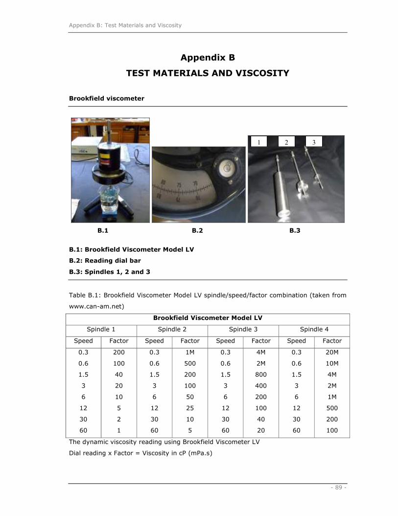
Appendix B: Test Materials and Viscosity
- 89 -
Appendix B
TEST MATERIALS AND VISCOSITY
Brookfield viscometer
B.1 B.2 B.3
B.1: Brookfield Viscometer Model LV
B.2: Reading dial bar
B.3: Spindles 1, 2 and 3
Table B.1: Brookfield Viscometer Model LV spindle/speed/factor combination (taken from
www.can-am.net)
Brookfield Viscometer Model LV
Spindle 1 Spindle 2 Spindle 3 Spindle 4
Speed Factor Speed Factor Speed Factor Speed Factor
0.3
0.6
1.5
3
6
12
30
60
200
100
40
20
10
5
2
1
0.3
0.6
1.5
3
6
12
30
60
1M
500
200
100
50
25
10
5
0.3
0.6
1.5
3
6
12
30
60
4M
2M
800
400
200
100
40
20
0.3
0.6
1.5
3
6
12
30
60
20M
10M
4M
2M
1M
500
200
100
The dynamic viscosity reading using Brookfield Viscometer LV
Dial reading x Factor = Viscosity in cP (mPa.s)
1 2 3

Appendix B: Test Materials and Viscosity
- 90 -
Table B.2: Data results for apparent viscosity of CMC at different concentrations
and temperatures, T (oC)
Temperature CMC % w/w at T = 18oC
T (oC) 0.5 1.0 1.5
Apparent viscosity (Ns/m2)
14 0.186 0.991 2.093
16 0.160 0.817 1.710
18 0.150 0.712 1.523
20 0.145 0.654 1.445
22 0.141 0.600 1.360
Figure B.1: Apparent viscosity of 0.5% w/w CMC at different temperatures
The relationship between shear stress and shear rate using Ostwald-de Waele law:
n
dy
duk
=τ
Where, τ is the shear stress (Pa.s), k is the apparent viscosity (Ns/m2), dy
duis the velocity
profile (m/s) and n is the CMC flow behaviour index (0.47).

Appendix B: Test Materials and Viscosity
- 91 -
Table B.3: Data results for shear rate, ττττ of CMC at different concentration and
velocity gradient, dy
du (m/s)
CMC % w/w at T = 18oC CMC % w/w at T = 18oC
Velocity 0.5 1.0 1.5 Velocity 0.5 1.0 1.5
v (m/s) Shear stress, (Pa.s) v (m/s) Shear stress, (Pa.s)
0.00 0.000 0.000 0.000 1.30 0.170 0.805 1.723
0.10 0.051 0.241 0.516 1.40 0.176 0.834 1.784
0.20 0.070 0.334 0.715 1.50 0.181 0.861 1.843
0.30 0.085 0.404 0.865 1.60 0.187 0.888 1.899
0.40 0.098 0.463 0.990 1.70 0.192 0.914 1.954
0.50 0.108 0.514 1.100 1.80 0.198 0.939 2.008
0.60 0.118 0.560 1.198 1.90 0.203 0.963 2.059
0.70 0.127 0.602 1.288 2.00 0.208 0.986 2.110
0.80 0.135 0.641 1.371 2.10 0.213 1.009 2.158
0.90 0.143 0.678 1.449 2.20 0.217 1.031 2.206
1.00 0.150 0.712 1.523 2.30 0.222 1.053 2.253
1.10 0.157 0.745 1.593 2.40 0.226 1.074 2.298
1.20 0.163 0.776 1.659 2.50 0.231 1.095 2.343
For power law fluid (non-Newtonian and time-independent), Metzner and Reed (1955)
developed the Rabonowitsch-Mooney equation to:
γ
ρ nn
RM
VD−
=2
Re Eq. 8
and
18.* −= nkγ Eq. 9
n
n
nkk
+=
4
31* Eq. 10
Where,
k* = Non-Newtonian fluid consistency index,
n = Non-Newtonian flow behaviour index, 0.47 (Tonkin, 2004)

Appendix B: Test Materials and Viscosity
- 92 -
Equations 8 – 10 for CMC Reynolds number:
ηρ Ducmc
cmc =Re Eq. B1
Where, u is the velocity profile (m/s), η is the apparent viscosity of CMC (Ns/m2) at
different concentrations, D is the internal diameter of pipe (0.05m), and ρ is the
density of CMC (1000 kg/m3).
The data for CMC Reynolds number is shown in Table B.4.
Table B.4: Reynolds number for CMC at different concentrations and shear rates
depends on velocity requirements. Average temperatures were 18oC.
CMC % w/w at T = 18oC
Velocity 0.5 1.0 1.5
v (m/s) Shear rate, I
0.150 0.732 1.660
Reynolds number
0.20 66.67 13.66 6.02
0.40 133.33 27.32 12.05
0.50 166.67 34.15 15.06
0.60 200.00 40.98 18.07
0.80 266.67 54.64 24.10
1.00 333.33 68.31 30.12
1.20 400.00 81.97 36.14
1.40 466.67 95.63 42.17
1.50 500.00 102.46 45.18
1.60 533.33 109.29 48.19
1.80 600.00 122.95 54.22
2.00 666.67 136.61 60.24
2.50 833.33 170.77 75.30
The Reynolds numbers for CMC were exhibited within laminar flow.

Appendix C: Experimental Data
- 93 -
Appendix C
EXPERIMENTAL DATA
C.1 Calculation procedures for pressure drop
1. Determine the Reynolds number (Newtonian fluid)
µρ Du
v
Du ××=
×=Re Eq.15
2. Pipe friction coefficient
For laminar flow, the pipe friction coefficient, f (Hagen-Poiseuille equation):
Re
64=f Re ≤ 2000 Eq.20
For turbulent flow, the pipe friction coefficient, f (Colebrook equation, 1939):
+−=
Dff 7.3Re
256.1log4
1 ε Re ≥ 5000 Eq.21
3. Head loss
The pressure head loss (friction head), Pf is required to overcome the resistance of
fluid to flow in pipe and fittings. From equation 11 and 12, the friction head loss, f in
a length of pipe is given by:
g
u
D
LfPf
2
2
××= Eq.23
4. Pressure by vertical elevation (pressure-height relation)
hf PPP += Eq.24
Where, Ph = ρ.g.Hn Eq.25
5. Pressure drop, ∆P (Pa)
∆Pn,n+1 = Pn – Pn+1 Eq.26

Appendix C: Experimental Data
- 94 -
C.2 Pressure drop calculation for water
Condition (ONE 4-lobe swirl pipe):
Density of water, ρw (at 18oC) = 998.36 kg/m3
Viscosity of water µw (at 18oC) = 1.063x10⁻³ Ns/m2
Relative roughness, ε = 0.045 mm.
Velocity, v = 0.5 m/s
Reynolds number (Eq.15):
31.2347110063.1
5.005.0998Re
35.0 =×
××=
− (Turbulent)
Friction factor, f and rearrange Eq.21:
2
9.0Re
74.5
7.3log25.0
−
+= Df
ε
Eq.27
02705.023471
74.5
7.3
05.0
10045.0
log25.0
2
9.0
3
=
+
×
=
−−
f
Pressure head loss, Pf to overcome the friction factor, f (Eq.23):
247.02
5.0
05.0
8.3502705.0
2
=××=g
Pf Pa
The elevations, H (m) obtained from simple manometer tubes at 0.5m/s:
H1 = 6.740m
H2 = 6.738m
H3 = 5.818m
Pressure, P (Pa) (Eq.25):
P1 = 66010.96 Pa
P2 = 65991.38 Pa
P3 = 56980.98 Pa

Appendix C: Experimental Data
- 95 -
Therefore, the pressure drop, ∆P for water without swirl-inducing pipe (Eq.26):
∆P12 = P1 – P2 = 66010.96 – 65991.38 = 19.58 Pa (~ 20 Pa)
∆P23 = P2 – P3 = 65991.38 – 56980.98 = 9010.40 Pa (~ 9010 Pa)
∆P13 = P1 – P2 = 66010.96 – 56980.98 = 9029.98 Pa (~ 9030 Pa)
Table C.3: Flow rate, velocity, height of manometer tube and pressure drop data
for water with and without swirl inducing pipe
Flowrate Velocity
Average
Frequency
Average
T
Average height, H (m)
manometer tube
Data
Q
(m3/hr) V (m/s) F (Hz) oC K H1 H2 H3
3.534 0.5 9.35 18.2 291.2 6.743 6.738 5.818
7.069 1.0 12.25 18.2 291.2 6.288 6.258 5.333
10.603 1.5 16.30 18.4 291.4 6.593 6.528 5.593
14.137 2.0 20.60 18.6 291.6 7.053 6.938 5.988
2
Swirls
17.672 2.5 25.15 18.7 291.7 7.588 7.418 6.463
3.534 0.5 9.35 18.2 291.2 7.588 7.418 6.463
7.069 1.0 12.30 18.3 291.3 7.053 6.938 5.988
10.603 1.5 16.35 18.5 291.5 6.593 6.528 5.593
14.137 2.0 20.65 18.5 291.5 6.288 6.258 5.333 1 Swirl
17.672 2.5 25.15 18.6 291.6 6.743 6.738 5.818
3.534 0.5 9.40 18.3 291.3 6.744 6.738 5.817
7.069 1.0 12.30 18.4 291.4 6.287 6.257 5.332
10.603 1.5 16.40 18.6 291.6 6.592 6.525 5.592
14.137 2.0 20.70 18.7 291.7 7.054 6.939 5.987
No
swirl
17.672 2.5 25.20 18.9 291.9 7.598 7.419 6.465
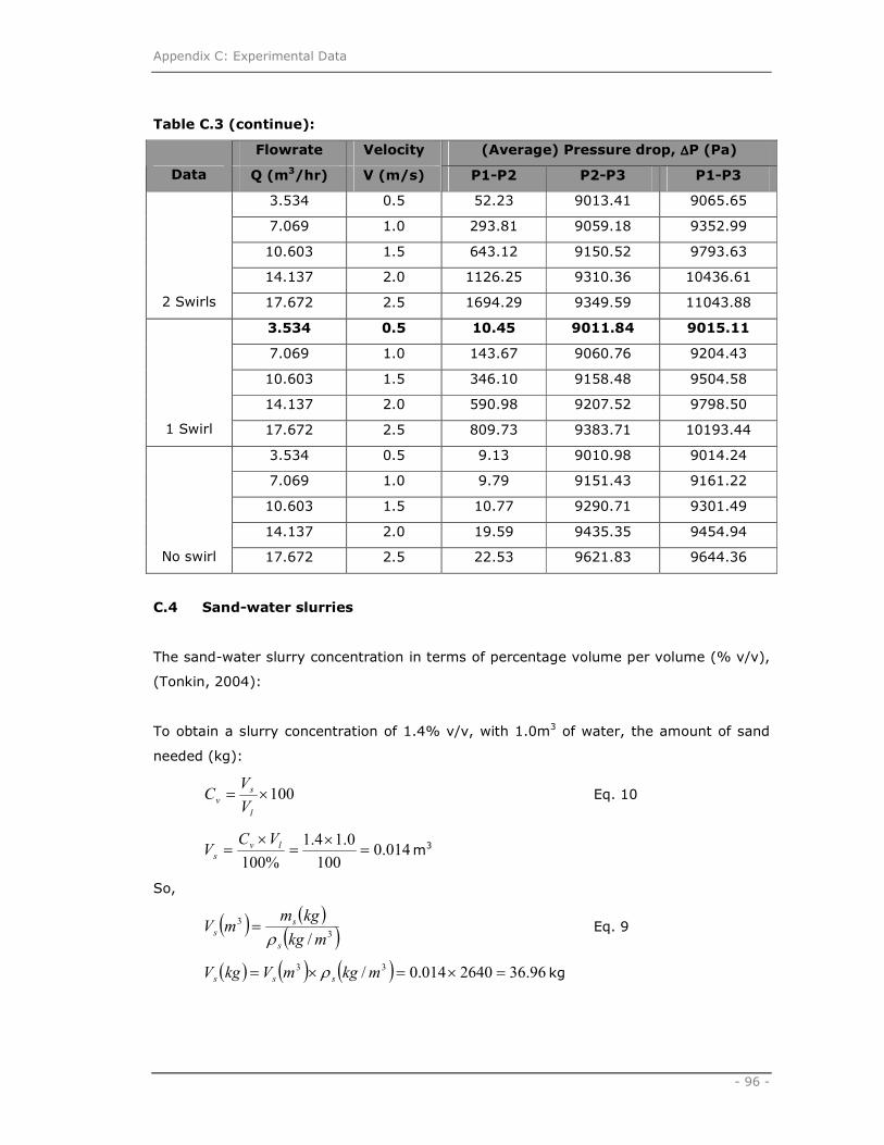
Appendix C: Experimental Data
- 96 -
Table C.3 (continue):
Flowrate Velocity (Average) Pressure drop, ∆∆∆∆P (Pa)
Data Q (m3/hr) V (m/s) P1-P2 P2-P3 P1-P3
3.534 0.5 52.23 9013.41 9065.65
7.069 1.0 293.81 9059.18 9352.99
10.603 1.5 643.12 9150.52 9793.63
14.137 2.0 1126.25 9310.36 10436.61
2 Swirls 17.672 2.5 1694.29 9349.59 11043.88
3.534 0.5 10.45 9011.84 9015.11
7.069 1.0 143.67 9060.76 9204.43
10.603 1.5 346.10 9158.48 9504.58
14.137 2.0 590.98 9207.52 9798.50
1 Swirl 17.672 2.5 809.73 9383.71 10193.44
3.534 0.5 9.13 9010.98 9014.24
7.069 1.0 9.79 9151.43 9161.22
10.603 1.5 10.77 9290.71 9301.49
14.137 2.0 19.59 9435.35 9454.94
No swirl 17.672 2.5 22.53 9621.83 9644.36
C.4 Sand-water slurries
The sand-water slurry concentration in terms of percentage volume per volume (% v/v),
(Tonkin, 2004):
To obtain a slurry concentration of 1.4% v/v, with 1.0m3 of water, the amount of sand
needed (kg):
100×=l
s
vV
VC Eq. 10
014.0100
0.14.1
%100=
×=
×= lv
s
VCV m3
So,
( ) ( )( )3
3
/mkg
kgmmV
s
s
s ρ= Eq. 9
( ) ( ) ( ) 96.362640014.0/ 33 =×=×= mkgmVkgV sss ρ kg

Appendix C: Experimental Data
- 97 -
The sand needed is approximately 37.0 kg.
At 18°C, the density of water is approximately 998.0 kg/m3. Therefore, the density of
sand-water slurry, ρm (kg/m3) (Nesbitt, 2000) equation 12:
( ) ( )0.1021
100
0.9980.26404.10.998
100=
−+=
−+= lsv
lm
C ρρρρ kg/m3
Table C.6: Sand-water slurries concentrations
Volume Total Density of
Concentration of solids Sand volume slurries
C1 (% v/v) Water (L) L Kg VT (L) ρρρρ (kg/m3)
1.4 986.19 13.81 36.45 1000 1022.96
2.1 979.43 20.57 54.30 1000 1034.44
2.7 973.71 26.29 69.41 1000 1044.28
C.7 Pressure drop calculation for sand-water slurry
Condition (ONE 4-lobe swirl pipe):
Concentration of sand-water slurry = 1.4% v/v
Density of mixture, ρm (at 18oC) = 1021.0 kg/m3
Viscosity of mixture, µm (at 18oC) = 1.063x10⁻³ Ns/m2
Relative roughness, ε = 0.045 mm.
Velocity, v = 0.5 m/s
Assumption:
Viscosity of mixture, µm is the same as viscosity of water, µw at given temperature
condition.
Pressure, P (Pa) values for P1, P2 and P3 when used one 4-lobe swirl-inducing pipe at
nominal velocity of 0.5 m/s were calculated as follows:
Reynolds number (Eq.15):
2.2401210063.1
5.005.00.1021Re
35.0 =×
××=
− (Turbulent)

Appendix C: Experimental Data
- 98 -
Friction factor, f Eq.27:
175.124012
74.5
7.3
05.0
10045.0
log25.0
2
9.0
3
=
+
×
=
−−
f
Pressure head loss, Pf to overcome the friction factor, f (Eq.23):
72.102
5.0
05.0
8.35175.1
2
=××=g
Pf Pa
The elevations, H (m) from simple manometer tubes at 0.5m/s
H1 = 7.533 m
H2 = 7.511 m
H3 = 6.574 m
Pressure, P (Pa) (Eq.25):
P1 = 75450.60 Pa
P2 = 75230.18 Pa
P3 = 65845.18 Pa
Therefore, the pressure drop, ∆P for water without swirl-inducing pipe (Eq.26):
∆P12 = P1 – P2 = 220.42 Pa (~ 220 Pa)
∆P23 = P2 – P3 = 9385.00 Pa (~ 9400 Pa)
∆P13 = P1 – P2 = 9605.42 Pa (~ 9600 Pa)

Appendix C: Experimental Data
- 99 -
Table C.8: Flow rate, velocity, height of manometer tube and pressure drop data
for sand-water slurries with and without swirl inducing pipe
(Average) Frequency, F (Hz)
Water Sand-water % v/v
Flow rate Velocity 1.4 2.1 2.7
(Average)
Temperature, T Data
Q (m3/hr) V (m/s) 800L 30.0 kg 45.3 kg 58.6 kg oC K
3.534 0.5 9.35 9.40 9.50 9.60 18.6 291.6
7.069 1.0 12.25 12.30 12.50 12.50 18.6 291.6
10.603 1.5 16.30 16.30 16.50 16.70 18.7 291.7
14.137 2.0 20.60 18.70 21.00 21.40 18.8 291.8 2 Swirl
17.672 2.5 25.15 23.80 25.50 26.10 18.9 291.9
3.534 0.5 9.35 9.50 9.50 9.60 18.8 291.8
7.069 1.0 12.30 12.40 12.60 12.70 18.9 291.9
10.603 1.5 16.35 16.50 16.80 17.00 18.9 291.9
14.137 2.0 20.65 20.70 21.80 22.10 19.0 292.0 1 Swirl
17.672 2.5 25.15 25.40 26.10 26.80 19.0 292.0
3.534 0.5 9.40 9.50 9.60 9.60 18.4 291.4
7.069 1.0 12.30 12.50 12.70 12.80 18.6 291.6
10.603 1.5 16.40 16.70 17.00 17.20 18.6 291.6
14.137 2.0 20.70 20.80 22.00 22.40 18.7 291.7 No swirl
17.672 2.5 25.20 25.60 27.30 27.80 18.8 291.8

Appendix C: Experimental Data
- 100 -
Table C.8 (continue):
Average pressure drop, ∆∆∆∆P (Pa)
P1-P2 P2-P3 P1-P3 P1-P2 P2-P3 P1-P3 P1-P2 P2-P3 P1-P3
Velocity Sand-water % v/v Data
V (m/s) 1.4 2.1 2.7
0.5 500.99 9131.71 9632.71 507.55 9240.75 9748.30 521.13 9426.11 9947.25
1.0 1234.86 8933.65 10151.85 1238.43 9157.00 10395.42 1267.44 9340.13 10607.57
1.5 1657.88 9208.60 10836.01 1657.64 9503.74 11161.38 1690.73 9779.32 11470.05
2.0 1672.41 9964.93 11722.05 1792.35 10165.54 11957.89 1829.54 10469.07 12298.61 2 Swirl
2.5 1859.52 10710.18 12601.02 1926.79 11265.97 13192.77 1966.28 11358.40 13324.68
0.5 222.43 9390.15 9612.58 226.45 9577.98 9804.43 230.01 9657.48 9887.49
1.0 589.76 9268.35 9858.11 603.34 9451.78 10055.12 615.37 9529.29 10144.66
1.5 862.36 8979.21 10321.56 1142.37 9159.34 10528.16 1395.99 9342.43 10738.42
2.0 1301.35 9544.28 10845.63 1327.50 9734.80 11062.30 1354.02 10017.04 11371.06 1 Swirl
2.5 1377.01 10109.26 11486.27 1405.81 10310.75 11716.56 1434.12 10743.70 12177.82
0.5 19.66 9492.18 9511.84 16.20 9682.30 9700.86 19.78 9943.40 9963.18
1.0 79.73 9678.69 9758.42 80.85 9871.53 9952.38 83.24 10069.06 10152.30
1.5 141.63 9963.48 10105.11 145.18 10163.52 10308.70 147.19 10365.86 10513.05
2.0 211.18 10340.78 10551.96 215.34 10547.50 10762.84 219.56 10758.46 10978.02 No swirl
2.5 287.77 10760.18 11047.95 295.31 10975.82 11271.13 298.85 11195.10 11493.95
Average elevation, H (m) of manometer tube
H1 H2 H3 H1 H2 H3 H1 H2 H3
Velocity Sand-water % v/v Data
V (m/s) 1.4 2.1 2.7
0.5 7.505 7.455 6.541 7.436 7.386 6.471 7.380 7.329 6.405
1.0 7.038 6.917 6.025 6.985 6.863 5.959 7.003 6.878 5.956
1.5 7.360 7.198 6.283 7.311 7.148 6.213 7.338 7.172 6.210
2.0 7.894 7.717 6.718 7.829 7.652 6.643 7.860 7.678 6.639 2 Swirls
2.5 8.488 8.299 7.228 8.452 8.262 7.148 8.461 8.267 7.144
0.5 7.533 7.511 6.574 7.471 7.449 6.504 7.405 7.383 6.439
1.0 6.969 6.910 5.985 6.913 6.853 5.920 6.852 6.792 5.860
1.5 7.263 7.129 6.233 7.203 7.068 6.163 7.149 7.013 6.100
2.0 7.715 7.585 6.632 7.651 7.520 6.559 7.603 7.471 6.492 1 Swirl
2.5 8.260 8.123 7.114 8.192 8.053 7.035 8.153 8.013 6.963
0.5 6.786 6.784 5.837 6.732 6.730 5.775 6.691 6.689 5.717
1.0 7.010 7.002 6.036 6.954 6.946 5.971 6.905 6.896 5.912
1.5 7.333 7.319 6.325 7.275 7.261 6.257 7.223 7.208 6.195
2.0 7.765 7.744 6.712 7.703 7.681 6.640 7.647 7.625 6.574 No swirl
2.5 8.282 8.253 7.179 8.215 8.186 7.102 8.155 8.126 7.031

Appendix C: Experimental Data
- 101 -
y = 0.992x + 70.99y = x
8850
9350
9850
10350
10850
11350
8850 9350 9850 10350 10850 11350
∆P
23
∆P13 - ∆P12
Validation of ∆∆∆∆P23
Water 2.7% v/v slurry
Figure C.9: Graph to show the validation of ∆∆∆∆P23 against ∆∆∆∆P13 - ∆∆∆∆P12 for water and
sand-water slurry at 2.7% v/v
The swirl-inducing pipe caused lower pressure drops compared to when fluids were
preceded without the swirl-inducing pipe. The graph in figure C.9 shows a validation of
pressure drops for ∆P23. The overall pressure drop across the pipe rig was obtained from
∆P13, which was equal to ∆P12+∆P23. Therefore, the ∆P23 should be equal to ∆P13 - ∆P12.
The statistical data obtained and plotted for the effect of swirl inducing pipe flow over the
bend showed similarity in the gradient (approximately, m = 1) when ∆P23 was plotted
against ∆P12 - ∆P12. The ∆P23 data was obtained directly from the results (Table C:3 for
water and table C.8 for 2.7% v/v slurry) and plotted against the value of ∆P13 - ∆P12.
These results proved that the pressure drops obtained from the bend were acceptable.

Appendix C: Experimental Data
- 102 -
C.10 Carboxymethyl cellulose (CMC)
Reynolds number for CMC can be obtained in Appendix B.4. The pressure measurements
for 0.5% w/w CMC were obtained using equations 11 – 16. While, the pressure
measurements for 1.0 and 1.5% CMC were obtained directly from Bourdon gauge.
Table C.11: 0.5% w/w CMC
0.5 Q v ηηηη Heigh, H (m) Pressure different, DP (Pa)
% w/w (m3/hr) (m/s)
F
(Hz) T oC Ns/m2 H1 H2 H3 ∆∆∆∆P1 ∆∆∆∆P2 ∆∆∆∆P3
3.534 0.5 9.4 18.2 0.149 7.058 7.015 6.440 425.10 5509.95 6065.85
7.069 1.0 12.3 18.3 0.149 7.438 7.304 6.296 1313.45 8087.80 11199.75
10.603 1.5 16.4 18.3 0.149 7.298 7.062 6.083 2310.80 8452.95 11919.15 2 swirl
14.137 2.0 20.7 18.3 0.149 7.738 7.518 6.510 2158.20 9913.55 12049.95
3.534 2.0 9.4 18.3 0.149 7.078 7.050 6.496 272.50 5466.35 5706.15
7.069 1.5 12.3 18.4 0.149 7.278 7.229 6.392 485.05 8202.25 8688.12
10.603 1.0 16.4 18.4 0.149 7.438 7.322 6.381 1139.05 9232.30 10371.35 1 swirl
14.137 0.5 20.7 18.4 0.149 7.688 7.585 6.597 1013.70 9684.65 10698.35
3.534 0.5 13.4 18.2 0.149 7.098 7.085 6.547 130.80 5648.93 5403.68
7.069 1.0 17.7 18.3 0.149 7.238 7.226 6.290 114.45 8976.15 9303.15
10.603 1.5 21.2 18.3 0.149 7.398 7.373 6.285 245.25 9695.55 10917.71
No swirl 14.137 2.0 25.2 18.3 0.149 7.668 7.641 6.604 261.60 10186.05 10441.11
Table C.12: 1.0% w/w CMC
1.0% Q v F T ηηηη Ave pressure (psi) Pressure different, ∆∆∆∆P (Pa)
w/w (m3/hr) (m/s)
(Hz) oC
Ns/m2 P1 P2 P3 ∆∆∆∆P1 ∆∆∆∆P2 ∆∆∆∆P3
3.534 0.5 10.6 17.9 0.7199 7.8 7.5 7.0 1896.05 3619.75 5515.80
7.069 1.0 12.7 18.1 0.7091 8.1 7.6 7.0 2930.27 3619.75 6550.02
10.603 1.5 16.6 18.4 0.7004 8.4 7.8 7.1 4309.22 4826.33 9135.55
14.137 2.0 20.9 18.8 0.6903 9.0 8.2 7.3 4688.17 6205.28 11893.45 2 swirl
17.671 2.5 25.4 19.0 0.6821 10.6 9.6 8.4 6411.86 8273.71 15685.57
3.534 0.5 11.2 17.9 0.7199 8.2 8.0 7.6 1378.94 3102.64 4481.58
7.069 1.0 15.0 18.1 0.7091 8.6 8.4 8.0 1551.32 3619.75 5171.07
10.603 1.5 19.5 18.3 0.7033 9.2 8.8 8.4 2757.90 2585.53 5343.43
14.137 2.0 24.2 18.9 0.6874 9.8 9.3 8.6 3447.38 4481.59 7928.97 1 swirl
17.671 2.5 28.9 19.2 0.6763 11.0 10.4 9.0 4136.86 9652.66 13789.52
3.534 0.5 12.0 17.8 0.7225 9.5 9.4 8.8 689.47 4309.22 4998.70
7.069 1.0 17.6 18.1 0.7077 10.0 9.8 9.1 1551.32 4136.85 5688.17
10.603 1.5 22.5 18.4 0.7019 10.5 10.2 9.5 2413.17 4653.96 7067.13
14.137 2.0 27.3 18.7 0.6917 11.0 10.6 9.8 2585.54 5343.44 7928.97 No swirl
17.671 2.5 32.4 19.0 0.6836 12.0 11.5 10.1 3619.74 9307.92 12927.67

Appendix C: Experimental Data
- 103 -
Table C.13: 1.5% w/w CMC
Bourdon gauge
(Ave. psi) Pressure different, ∆∆∆∆P (Pa) 1.5
%w/w
Q
(m3/hr)
v
(m/s) F (Hz)
T
oC
ηηηη
Ns/m2 P1 P2 P3 ∆∆∆∆P1 ∆∆∆∆P2 ∆∆∆∆P3
1.414 0.2 7.5 17.6 1.5664 9.0 8.8 8.2 1378.95 3677.20 5056.15
2.827 0.4 9.8 17.6 1.5664 9.4 9.1 8.5 2068.43 4136.85 6205.29
4.241 0.6 12.1 17.7 1.5511 9.8 9.5 8.9 2068.43 4136.85 6205.28
5.655 0.8 14.4 17.8 1.5417 10.0 9.6 8.8 2757.90 5515.81 8273.71
7.069 1.0 16.6 17.9 1.5324 10.4 9.8 8.8 4136.85 6894.76 11031.61
8.482 1.2 18.9 18.1 1.5191 10.8 10.0 8.8 5515.81 8273.71 13789.51
9.896 1.4 20.7 18.4 1.5074 10.8 9.6 8.2 8273.71 9652.66 17926.37
11.310 1.6 22.9 18.6 1.4996 10.8 9.4 7.8 9652.66 11031.61 20684.28
12.723 1.8 25.3 18.7 1.4957 11.4 9.9 8.3 10342.14 11031.61 21373.75
2 swirl
14.137 2.0 27.4 18.7 1.4957 11.8 10.1 8.3 11721.08 12410.56 24131.65
1.414 0.2 7.8 17.6 1.5664 11.6 11.5 11.2 689.48 2068.43 2757.90
2.827 0.4 12.0 17.7 1.5511 13.6 13.4 13.0 1378.95 2757.90 4136.85
4.241 0.6 15.6 17.8 1.5417 15.0 14.7 14.1 2068.43 4136.85 6205.28
5.655 0.8 18.9 17.9 1.5324 16.0 15.6 14.8 2757.90 5515.81 8273.71
7.069 1.0 21.9 17.9 1.5324 17.2 16.6 15.6 4136.85 6894.76 11031.61
8.482 1.2 24.8 18.0 1.5230 18.0 17.2 16.1 5515.81 7584.23 13100.04
9.896 1.4 27.4 18.1 1.5191 18.8 17.8 16.6 6894.76 8273.71 15168.46
11.310 1.6 30.0 18.6 1.4996 19.8 18.6 17.2 8273.71 9652.66 17926.37
12.723 1.8 32.6 18.6 1.4996 20.0 18.6 17.1 9652.66 10342.14 19994.80
1 swirl
14.137 2.0 35.2 18.6 1.4996 20.4 18.8 17.1 11031.61 11261.44 22293.04
1.414 0.2 7.9 18.1 1.5191 12.0 11.9 11.6 459.65 1838.60 2298.25
2.827 0.4 12.1 18.2 1.5152 14.0 13.9 13.6 919.30 1838.60 2757.90
4.241 0.6 15.8 18.2 1.5152 15.8 15.6 15.3 1378.95 2068.43 3447.38
5.655 0.8 19.1 18.2 1.5152 17.0 16.8 16.4 1378.95 2757.90 4136.86
7.069 1.0 22.1 18.2 1.5152 18.0 17.8 17.3 1378.96 3447.38 4826.33
8.482 1.2 24.9 18.2 1.5152 19.0 18.7 18.1 2298.25 3907.03 6205.28
9.896 1.4 27.6 18.3 1.5113 19.8 19.4 18.8 2757.90 4136.85 6894.76
11.310 1.6 30.2 18.3 1.5113 20.0 19.5 18.8 3217.55 5056.16 8273.71
12.723 1.8 32.8 18.4 1.5074 20.5 19.9 19.0 3907.03 6435.11 10342.14
No swirl
14.137 2.0 35.4 18.4 1.5074 21.0 20.3 19.1 4826.33 8273.71 13100.04

Appendix C: Experimental Data
- 104 -
C.14 Pressure drop, ∆∆∆∆P12 (Pa) against velocity, v (m/s) for CMC at 1.5% w/w
P1-P2, 1.5% w/w CMC
0
2000
4000
6000
8000
10000
12000
14000
0.0 0.5 1.0 1.5 2.0 2.5
Velocity, v (m/s)
Pre
ssure
dro
p,
∆P (
Pa)
The pressure drops, ∆P12 (Pa) for 1.5% w/w CMC were increased when the velocity, v
(m/s) increasing. The swirl-inducing pipe gave higher pressure drops compared to the
CMC fluid flows without proceeded swirl-inducing pipe. At 0.2m/s, the pressure drops for
2 swirls, 1 swirl and no swirl were approximately at 1400Pa, 700Pa and 460Pa
respectively. At 1.0m/s, the pressure drops were approximately at 4100Pa, 4100Pa and
1400Pa respectively. At 2.0m/s, the pressure drops were approximately at 12000Pa,
11300Pa and 8300Pa respectively.
C.15 Pressure drop, ∆∆∆∆P23 (Pa) for CMC at over the bend (R/D of 4)
P2-P3, 1.5% w/w CMC
0
2000
4000
6000
8000
10000
12000
14000
0.0 0.5 1.0 1.5 2.0 2.5 3.0
Velocity, v (m/s)
Pre
ssure
dro
p,
∆P (
Pa)
The pressure drops, ∆P23 over the bend for 1.5% w/w CMC proceeded with swirl-inducing
pipe were higher compared to a flow without swirl-inducing pipe. Due to its higher
apparent viscosity, the ∆P23 over the bend has similar graph trends with ∆P12 (C.12) and
∆P13 (Figure 5.14 c).
P1 P3P2
R/D=4
Directionof flowPressure devices
Swirl pipe
P1 P3P2
R/D=4
Direction
of flowPressure devices
Swirl pipe
2 swirls
1 swirl
No swirl
2 swirls
1 swirl
No swirl