Embed Size (px)
Citation preview
U.S. Department of the Interior Bureau of Reclamation Technical Services Center
Seismotectonics and Geophysics Group December 2012
Technical Memorandum No. TM-86-68330-2012-23
Geophysical Investigations Electrical Resistivity Surveys Santee Basin Aquifer Recharge Study Santee, California
Phase 2 Report Lower Colorado Region, Southern California Area Office
For official use only

United States Department of the Interior Mission Statement
The mission of the Department of the Interior is to protect and provide access to
our Nation’s natural and cultural heritage and honor our trust responsibilities to
Indian Tribes and our commitments to island communities.
Bureau of Reclamation Mission Statement
The mission of the Bureau of Reclamation is to manage, develop, and protect
water and related resources in an environmentally and economically sound
manner in the interest of the American public.
Technical Memorandum TM-86-68330-2012-23
Geophysical Investigations Electrical Resistivity Surveys
Santee Basin Aquifer Recharge Study Phase 2 Report
Lower Colorado Region, Southern California Area Office Prepared by: /s/ Kristen S. Pierce 28-Dec-2012 ______________________________________ ___________________ Kristen S. Pierce Date Geophysicist /s/ Daniel J. Liechty 28-Dec-2012 ______________________________________ ___________________ Daniel J. Liechty Date Geophysicist /s/ Justin B. Rittgers 28-Dec-2012 ______________________________________ ___________________ Justin B. Rittgers Date Geophysicist Peer Review by: /s/ Richard D. Markiewicz 28-Dec-2012 ______________________________________ _____________________ Richard D. Markiewicz Date Team Lead, Geophysics of the U.S. Department of the Interior Bureau of Reclamation Technical Service Center Seismotectonics and Geophysics Group
TM-86-68330-2112-23
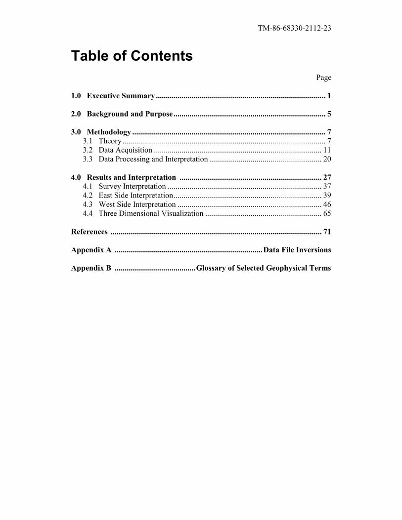
Table of Contents
Page
1.0 Executive Summary ...................................................................................... 1
2.0 Background and Purpose ............................................................................. 5
3.0 Methodology .................................................................................................. 7
3.1 Theory ....................................................................................................... 7
3.2 Data Acquisition ..................................................................................... 11
3.3 Data Processing and Interpretation ......................................................... 20
4.0 Results and Interpretation ........................................................................ 27
4.1 Survey Interpretation .............................................................................. 37
4.2 East Side Interpretation ........................................................................... 39
4.3 West Side Interpretation ......................................................................... 46
4.4 Three Dimensional Visualization ........................................................... 65
References ........................................................................................................... 71
Appendix A ........................................................................... Data File Inversions
Appendix B ......................................... Glossary of Selected Geophysical Terms
TM-86-68330-2112-23
1
1.0 Executive Summary
Southern California water supplies originate mainly from Northern California, the Colorado
River system and local groundwater. Over the past ten years, there have been droughts and other
interruptions throughout these water supply locations. Padre Dam Municipal Water
District (Padre Dam or District) is seeking ways to increase local water supplies to ensure supply
reliability for their 100,000 customers. One such idea is injecting full advanced treated recycled
water into the Santee Basin aquifer, and following the appropriate residence time, extract it for
potable use. Padre Dam’s goal is to supply up to 15 percent of its projected 2020 water demands
through local water production. The District’s projected 2020 potable water supply needs, as
identified in their Urban Water Management Plan, is estimated to be 15,910 acre-feet per year
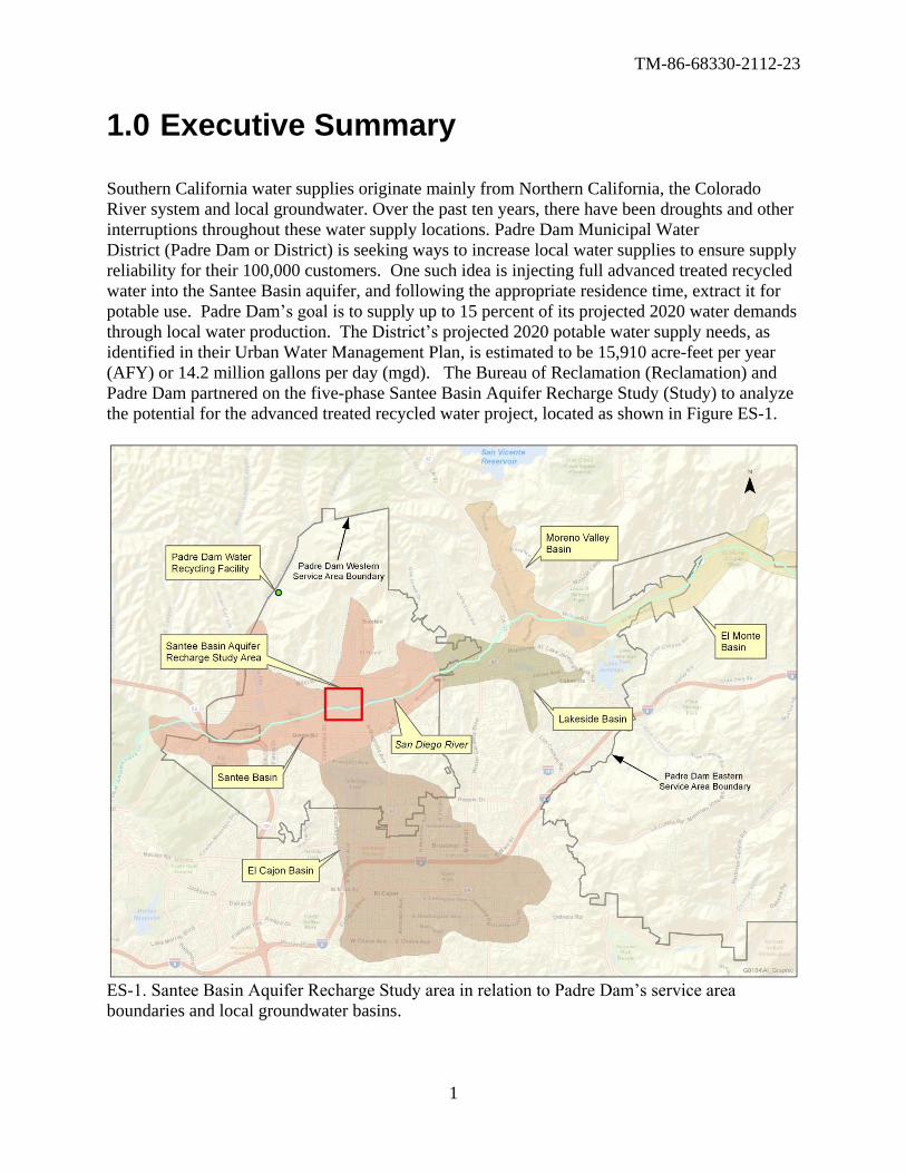
(AFY) or 14.2 million gallons per day (mgd). The Bureau of Reclamation (Reclamation) and
Padre Dam partnered on the five-phase Santee Basin Aquifer Recharge Study (Study) to analyze
the potential for the advanced treated recycled water project, located as shown in Figure ES-1.
ES-1. Santee Basin Aquifer Recharge Study area in relation to Padre Dam’s service area
boundaries and local groundwater basins.
TM-86-68330-2112-23
2
This Technical Memorandum (TM) 86-68330-2012-23 presents the Phase 2 Study results. Phase
1 study of the aquifer was completed in October 2011 and included a literature review and
interpretation, regulatory viability and engineering viability.
The Phase 1 TM presented the following results and recommendations:
The project site has potential as a full advanced recycled water recharge project site,
pending further studies.
Although the alluvium appeared shallower on the northern and southern fringe of the
subject site, the alluvial troughs below the San Diego River and to the south of the San
Diego River are deeper.
The yield of the Santee Basin aquifer was estimated to range from very small up to 3 mgd
depending on the composition of the aquifer material assumed (how fine or coarse).
The aquifer yield was calculated based on a 24 month retention time in the basin. It is
anticipated that the retention time can be reduced as more refined information on the
aquifer is developed in future phases.
Additional Study phases should occur to further refine data and analyses. Recommended
that the next phase define the bedrock topography through geophysical methods.
Given the results and recommendations of Phase 1, Phase 2 of the Santee Basin Aquifer
Recharge Study was undertaken. The primary objective in Phase 2 was to define the bedrock
topography through geophysical methods, such as electrical resistivity or seismic testing.
Electrical resistivity imaging (ERI) was chosen for the Phase 2 study. This Phase 2 TM presents
information about the ERI surveys conducted in March of 2012 by the Bureau of Reclamation,
with assistance from Padre Dam.
The purpose of the ERI surveys was to gain a better understanding of the depth to bedrock in the
Study area in order to help refine the aquifer volume determination. Well data from the area is
limited and depth to bedrock in the wells is inconsistent. Some wells indicate that bedrock depths
are as shallow as 25 feet and other wells indicate bedrock depths at 120 feet. The ERI surveys
were able to detect a contrast in electrical resistivity properties at, or near, the assumed physical
top of weathered granite bedrock surface. This conclusion is based upon a comparison of ERI
results and drilling results in the eastern portion of the survey area, as explained in the TM.
The proposed project area is located in an urban environment consisting of a mixture of man-
placed fill materials and natural deposits, which presented some complexity when analyzing the
ERI surveys’ results. In general, the distinction between natural and man-placed fill was
generally divided between the eastern and western sides of the survey area.
The ERI data collected on the east side of the survey area resulted in resistivity values showing a
strong resistivity contrast at depths corresponding to top of weathered granitic bedrock in nearby
wells. This means the interpreted depth to bedrock based on resistivity results can be defined
with a greater degree of confidence on the east side of the survey area.
The ERI data collected on the west side of the survey area had subsurface resistivity values of an
order of magnitude less than generally accepted resistivity values for the types of geologic
material suspected to exist in the area. Data collected on the west side of the survey area had to
TM-86-68330-2112-23
3
be re-scaled in order to recover any meaningful information beneath the man-placed fill
materials. Additional testing on the west side of the survey area is recommended to further
calibrate the ERI results and to better define depth to bedrock.
In general, bedrock in the survey area is shallower on the northern and eastern portions and
deeper in the western and southern portions. The bedrock depth is seen to be quite variable over
relatively short distances. The depth to bedrock in the survey area ranges from 70 feet to 140
feet below the ground surface (elevations of 270 to 200 feet), with the majority of the bedrock
beneath the Study area lying between 100 to 120 feet deep. Compared with the Phase 1 TM
estimated range of depth to bedrock, 40 feet to 140 feet, it appears that there is more aquifer
storage available to convey water. The refinement of depth to bedrock in Phase 2 should result
in a project yield higher than was estimated in Phase 1.
There are some isolated features within the ERI data results, which indicate there could be local
areas with much deeper, or much shallower, bedrock. The data coverage and resolution over
these isolated features is insufficient to make any definite interpretations as to bedrock depth at
those locations. These features may be due to near surface variations that have caused data
inversions resulting in difficulties in interpreting ERI results. Because these features are not
entirely resolved by the ERI surveys presented here, independent data such as from drilling, is
required and recommended to resolve these ambiguities.
It is important to note that the actual elevation of the groundwater surface is not detectable with
the technology used in this study. The blue color shown in the figures was selected not because
there is presence of water but rather illustrates the results of conductivity of the material
measured in the field.
Recommendations for Study next steps include:
Phase 3 – Targeted drilling to further calibrate the ERI results and determine hydraulic
conductivities and transmissivities
Phase 4 – Development of a detailed Groundwater Management Plan
Phase 5 – Development of injection and extraction wells placements and operating
strategies.
Phase 2 Study refinements predict the depth to bedrock indicated by the ERI surveys to be
greater than in the Phase 1. It is anticipated the yield of the aquifer could be higher than what
was estimated previously. As a result, Padre Dam is considering implementation of an aquifer
demonstration project. The objectives of the demonstration project are to collect engineering,
hydrogeologic, water quality, and injection well operational data to support the design and
permitting of a future full-scale, multi-well project.

TM-86-68330-2112-23
4
This page intentionally left blank.
TM-86-68330-2112-23
5
2.0 Background and Purpose This report details a geophysical survey conducted by the Bureau of Reclamation
in conjunction with the Padre Dam Municipal Water District as part of the Santee
Basin Aquifer Recharge Study. The purpose of this geophysical survey was to
characterize the location and configuration of weathered granitic bedrock units
which underlie alluvial sediments in the San Diego River valley, in particular
within the Santee Basin. This basin is located in eastern San Diego County, along
the San Diego River. The Padre Dam Municipal Water District is interested in this
area as the possible location of an indirect potable reuse project.
From March 13 through March 22, 2012, personnel from the Bureau of
Reclamation, Technical Service Center, and the Padre Dam Municipal Water
District and Reclamation’s Lower Colorado Region, Southern California Area
Office, completed 28 Electrical Resistivity Imaging (ERI) profiles in an area of
Santee, California that encompasses undeveloped land parcels as well as
redeveloped recreational open space.
The survey area is roughly bounded on the east and west by North Magnolia
Avenue and Cuyamaca Street and on the north and south by Riverwalk Drive and
Mission Gorge Road (Figure 1). The area is intersected from east to west by the
San Diego River.
The geophysical work completed at the survey area is presented and interpreted in
this Technical Memorandum (TM). The results of the ERI surveys give an
understanding of subsurface electrical properties at the project site, which can be
used as a proxy for multiple geologic and groundwater properties. ERI data can
allow for interpretation at depth between geologic formations of contrasting
electrical properties. A detailed analysis of the Santee Basin Aquifer was
completed using information about the local geology, surrounding well data, and
the ERI data collected during the study.
The results presented in this TM comprise bulk electrical resistivity values versus
depth over a series of profile lines conducted at the study site. There is a good
correlation between electrical resistivity and assumed top of weathered granitic
bedrock at the eastern half of the site. However, the western portion of the study
area contains an electrical resistivity structure which is markedly different than
the eastern portion. Therefore, as is shown in this TM, the correlation between
resistivity values and geologic interpretation (i.e. top of weathered granitic
bedrock) is not as straight forward as is observed on the eastern side of the site,
given the absence of further independent west-side site data such as well log
information.

TM-86-68330-2112-23
6
Figure 1: Location of survey area for the Santee Basin Aquifer Recharge Study.
The survey area is located approximately 14 miles northeast of the city of San
Diego, California, in the community of Santee.
TM-86-68330-2112-23
7
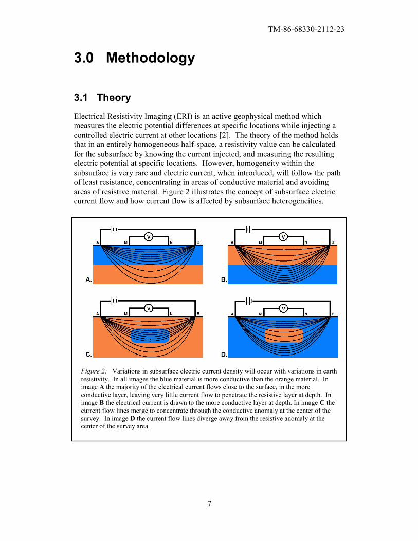
Figure 2: Variations in subsurface electric current density will occur with variations in earth
resistivity. In all images the blue material is more conductive than the orange material. In
image A the majority of the electrical current flows close to the surface, in the more
conductive layer, leaving very little current flow to penetrate the resistive layer at depth. In
image B the electrical current is drawn to the more conductive layer at depth. In image C the
current flow lines merge to concentrate through the conductive anomaly at the center of the
survey. In image D the current flow lines diverge away from the resistive anomaly at the
center of the survey area.
3.0 Methodology
3.1 Theory
Electrical Resistivity Imaging (ERI) is an active geophysical method which
measures the electric potential differences at specific locations while injecting a
controlled electric current at other locations [2]. The theory of the method holds
that in an entirely homogeneous half-space, a resistivity value can be calculated
for the subsurface by knowing the current injected, and measuring the resulting
electric potential at specific locations. However, homogeneity within the
subsurface is very rare and electric current, when introduced, will follow the path
of least resistance, concentrating in areas of conductive material and avoiding
areas of resistive material. Figure 2 illustrates the concept of subsurface electric
current flow and how current flow is affected by subsurface heterogeneities.
TM-86-68330-2112-23
8
Ohm’s Law describes electric current flow through a resistive material (equation
1). The basic concept of the law relates electric current (I) flowing through a
resistor to the voltage (V) applied across the resistor and the conductance of that
resistor. The inverse quantity of electrical conductance is electrical resistance
(R).
(1) I = V
R
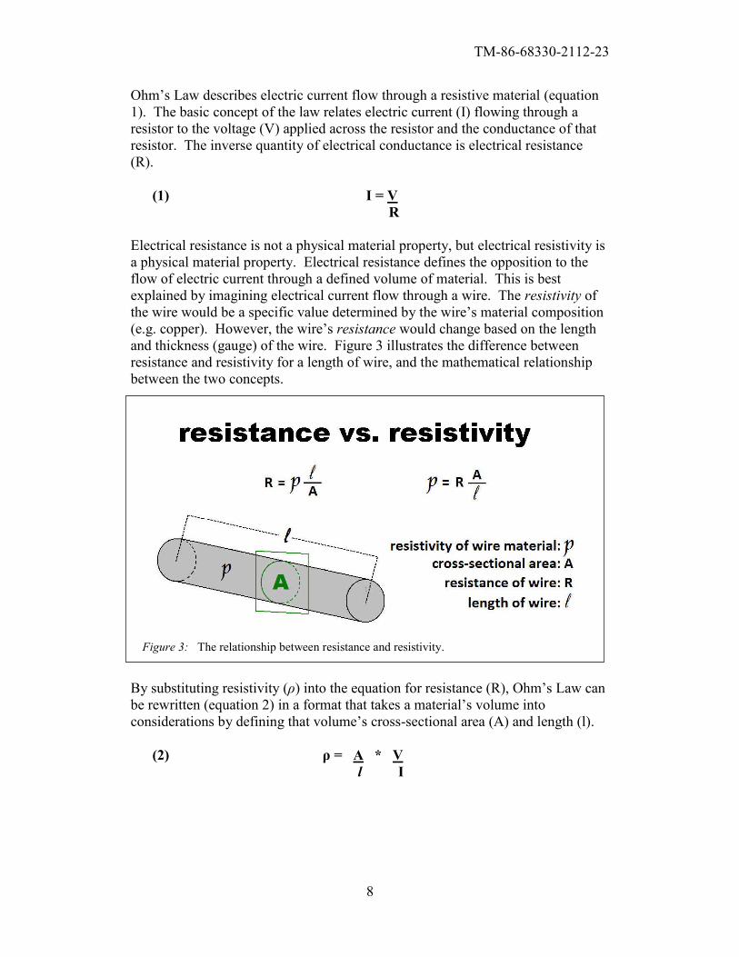
Electrical resistance is not a physical material property, but electrical resistivity is
a physical material property. Electrical resistance defines the opposition to the
flow of electric current through a defined volume of material. This is best
explained by imagining electrical current flow through a wire. The resistivity of
the wire would be a specific value determined by the wire’s material composition
(e.g. copper). However, the wire’s resistance would change based on the length
and thickness (gauge) of the wire. Figure 3 illustrates the difference between
resistance and resistivity for a length of wire, and the mathematical relationship
between the two concepts.
By substituting resistivity (ρ) into the equation for resistance (R), Ohm’s Law can
be rewritten (equation 2) in a format that takes a material’s volume into
considerations by defining that volume’s cross-sectional area (A) and length (l).
(2) ρ = A * V
l I
Figure 3: The relationship between resistance and resistivity.
TM-86-68330-2112-23
9
ERI aims to model the electrical resistivity structure of some volume of the earth.
From each ERI measurement, information is gained about the average electrical
resistance of a certain volume in the subsurface [3]. Variations in electrical
properties of subsurface materials make determination a true electrical resistivity
model of those materials nearly impossible [3]. Instead, the immediate quantity
calculated from an ERI survey is known as apparent resistivity (ρa). Apparent
resistivity can be thought of as a weighted average of all the true material
resistivities in the vicinity of the measurement. Apparent resistivity is calculated
using both current injected and electric potential measured, but also includes a
term that accounts for the relative positions of the current injection and potential
measurement electrodes, known as the geometric factor (K). The geometric
factor in ERI data processing can be compared conceptually to the wire’s length
and gauge in Figure 3 which relates resistance and resistivity in a three
dimensional space. By adapting Ohm’s law to account for the conditions specific
to ERI surveys, the basic equation of apparent resistivity can be derived (equation
3).
(3) ρa = K * V
I
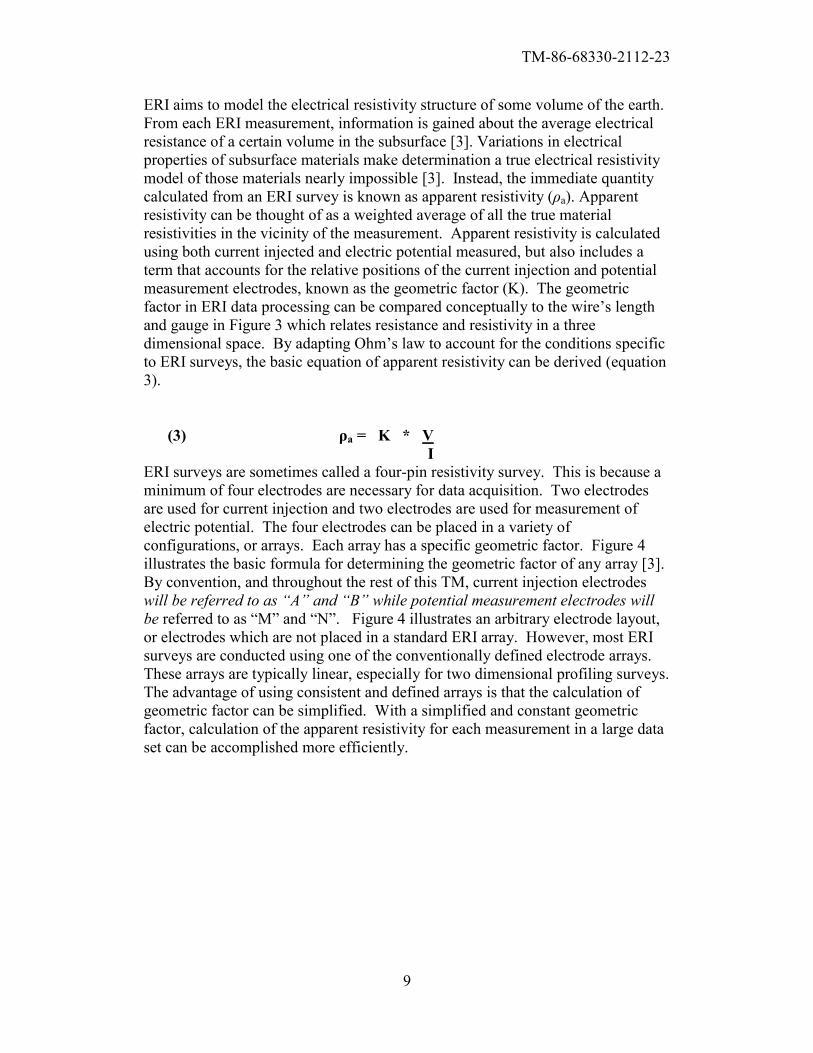
ERI surveys are sometimes called a four-pin resistivity survey. This is because a
minimum of four electrodes are necessary for data acquisition. Two electrodes
are used for current injection and two electrodes are used for measurement of
electric potential. The four electrodes can be placed in a variety of
configurations, or arrays. Each array has a specific geometric factor. Figure 4
illustrates the basic formula for determining the geometric factor of any array [3].
By convention, and throughout the rest of this TM, current injection electrodes
will be referred to as “A” and “B” while potential measurement electrodes will
be referred to as “M” and “N”. Figure 4 illustrates an arbitrary electrode layout,
or electrodes which are not placed in a standard ERI array. However, most ERI
surveys are conducted using one of the conventionally defined electrode arrays.
These arrays are typically linear, especially for two dimensional profiling surveys.
The advantage of using consistent and defined arrays is that the calculation of
geometric factor can be simplified. With a simplified and constant geometric
factor, calculation of the apparent resistivity for each measurement in a large data
set can be accomplished more efficiently.
TM-86-68330-2112-23
10
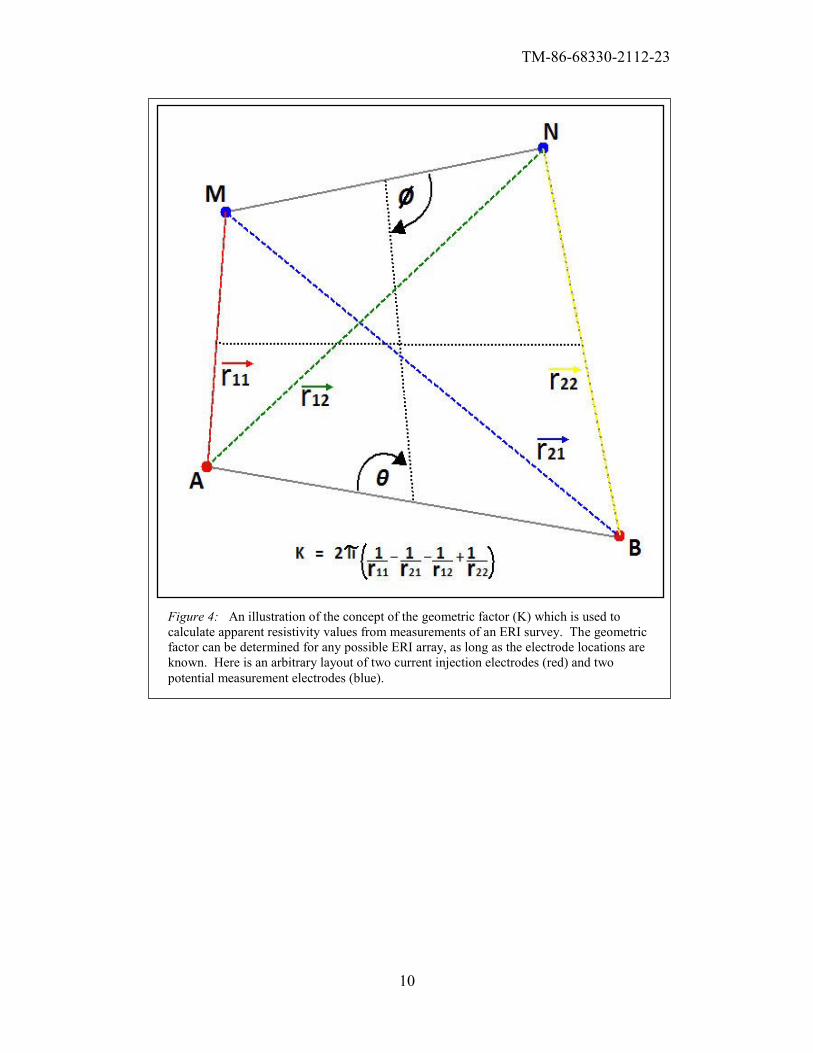
Figure 4: An illustration of the concept of the geometric factor (K) which is used to
calculate apparent resistivity values from measurements of an ERI survey. The geometric
factor can be determined for any possible ERI array, as long as the electrode locations are
known. Here is an arbitrary layout of two current injection electrodes (red) and two
potential measurement electrodes (blue).
TM-86-68330-2112-23
11
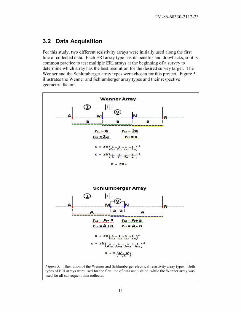
3.2 Data Acquisition
For this study, two different resistivity arrays were initially used along the first
line of collected data. Each ERI array type has its benefits and drawbacks, so it is
common practice to test multiple ERI arrays at the beginning of a survey to
determine which array has the best resolution for the desired survey target. The
Wenner and the Schlumberger array types were chosen for this project. Figure 5
illustrates the Wenner and Schlumberger array types and their respective
geometric factors.
Figure 5: Illustration of the Wenner and Schlumberger electrical resistivity array types. Both
types of ERI arrays were used for the first line of data acquisition, while the Wenner array was
used for all subsequent data collected.
TM-86-68330-2112-23
12
Both the Wenner and Schlumberger array types are relatively sensitive to vertical
variations in subsurface resistivity, but less sensitive to horizontal variations [4],
this tradeoff was considered beneficial for this survey location because semi-
lateral continuity of the geologic structure of the aquifer was expected. The
Wenner and Schlumberger arrays are generally known to have good signal
strength, because the electric potential measurement electrodes are located
between the current injection electrodes [4]. The time for data collection, as well
as data processing is generally greater for ERI data collected with the
Schlumberger array than the Wenner array. A field data quality comparison was
done for the data from the two different array types, and the Wenner array was
decided upon for data acquisition for the rest of the survey area.
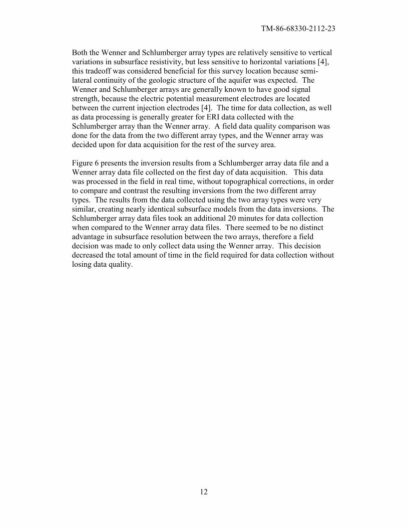
Figure 6 presents the inversion results from a Schlumberger array data file and a
Wenner array data file collected on the first day of data acquisition. This data
was processed in the field in real time, without topographical corrections, in order
to compare and contrast the resulting inversions from the two different array
types. The results from the data collected using the two array types were very
similar, creating nearly identical subsurface models from the data inversions. The
Schlumberger array data files took an additional 20 minutes for data collection
when compared to the Wenner array data files. There seemed to be no distinct
advantage in subsurface resolution between the two arrays, therefore a field
decision was made to only collect data using the Wenner array. This decision
decreased the total amount of time in the field required for data collection without
losing data quality.
TM-86-68330-2112-23
13
Figure 6: Field inversions of ERI data collected on the first day of geophysical data collection. The upper plot presents an inverted resistivity section of
data collected using the Schlumberger array while the results presented in the bottom plot utilized the Wenner array for data collection. More detail about
inverted resistivity sections is presented in section 3.0, data processing and interpretation. The two data files were collected at the same location using two
different array types. Both array types produced similar subsurface resistivity models. The Wenner array was chosen for this project because it had shorter
data acquisition time than the Schlumberger array.
TM-86-68330-2112-23
14
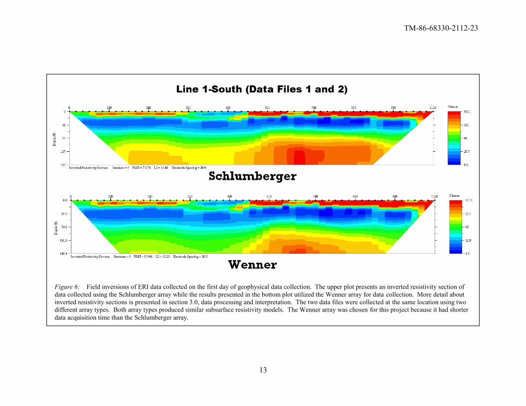
The ERI data at the Santee Basin Aquifer Recharge Study Site was acquired using
commercially available hardware, manufactured by Advanced Geosciences Inc.
(AGI), called a SuperSting™ Earth Resistivity Meter.* Positional data were
acquired at every other electrode location for all but one of the collected data
files. This data was acquired by IE Corporation, working under contract to Padre
Dam Water District.
The ERI surveys were conducted by installing a series of 56 stainless steel
electrodes into the ground. The electrodes are 18” long and generally installed to a
depth of one foot. The electrodes were connected by a cable to a computer-
controlled system unit. The computer was programmed with a file that designates
which electrodes to were used for current injection and which electrodes were
used for measurement of electrical potential difference. For any one data
measurement the system only uses four of the 56 electrodes. Figure 7 illustrates
instrumentation set-up for a typical ERI survey.
* Trade names and product names are given for information purposes only and do not constitute
endorsement by the U.S. Department of Interior – Bureau of Reclamation.
Figure 7: Illustration of ERI instrumentation set up for data collection.
TM-86-68330-2112-23
15
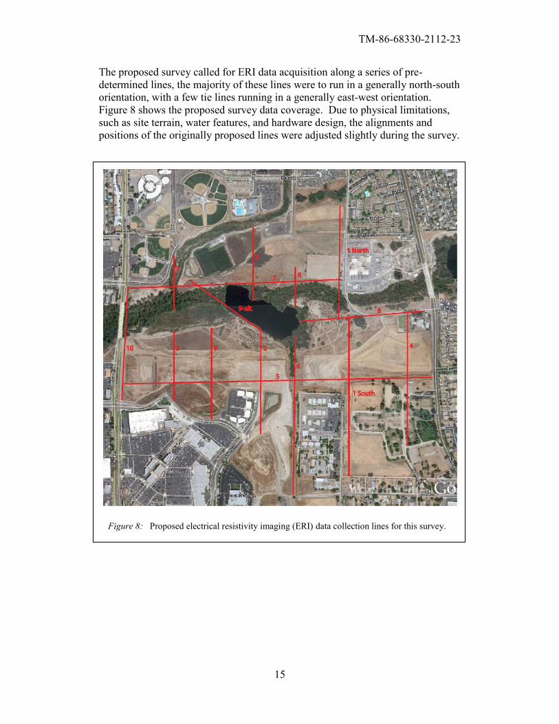
The proposed survey called for ERI data acquisition along a series of pre-
determined lines, the majority of these lines were to run in a generally north-south
orientation, with a few tie lines running in a generally east-west orientation.
Figure 8 shows the proposed survey data coverage. Due to physical limitations,
such as site terrain, water features, and hardware design, the alignments and
positions of the originally proposed lines were adjusted slightly during the survey.
Figure 8: Proposed electrical resistivity imaging (ERI) data collection lines for this survey.
TM-86-68330-2112-23
16
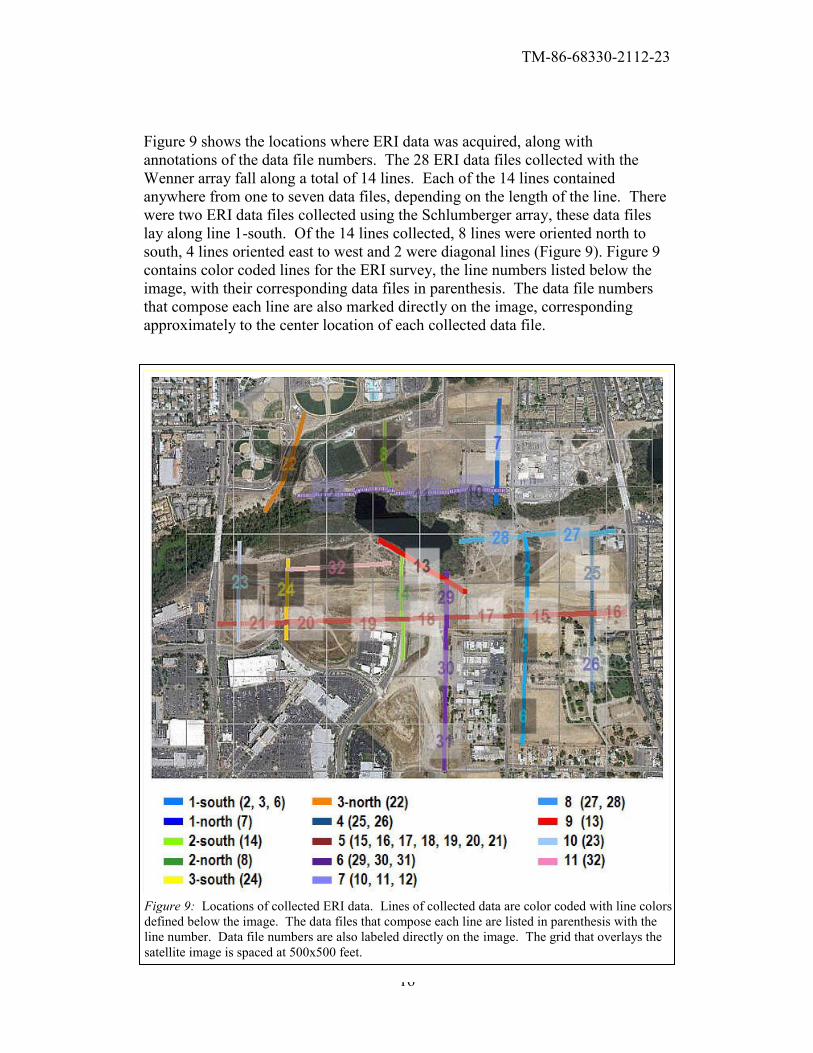
Figure 9 shows the locations where ERI data was acquired, along with
annotations of the data file numbers. The 28 ERI data files collected with the
Wenner array fall along a total of 14 lines. Each of the 14 lines contained
anywhere from one to seven data files, depending on the length of the line. There
were two ERI data files collected using the Schlumberger array, these data files
lay along line 1-south. Of the 14 lines collected, 8 lines were oriented north to
south, 4 lines oriented east to west and 2 were diagonal lines (Figure 9). Figure 9
contains color coded lines for the ERI survey, the line numbers listed below the
image, with their corresponding data files in parenthesis. The data file numbers
that compose each line are also marked directly on the image, corresponding
approximately to the center location of each collected data file.
Figure 9: Locations of collected ERI data. Lines of collected data are color coded with line colors
defined below the image. The data files that compose each line are listed in parenthesis with the
line number. Data file numbers are also labeled directly on the image. The grid that overlays the
satellite image is spaced at 500x500 feet.
TM-86-68330-2112-23
17
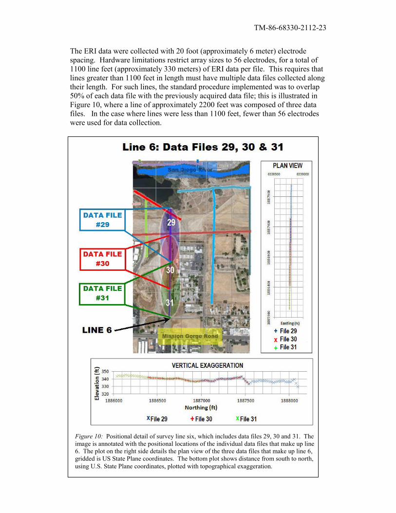
The ERI data were collected with 20 foot (approximately 6 meter) electrode
spacing. Hardware limitations restrict array sizes to 56 electrodes, for a total of
1100 line feet (approximately 330 meters) of ERI data per file. This requires that
lines greater than 1100 feet in length must have multiple data files collected along
their length. For such lines, the standard procedure implemented was to overlap
50% of each data file with the previously acquired data file; this is illustrated in
Figure 10, where a line of approximately 2200 feet was composed of three data
files. In the case where lines were less than 1100 feet, fewer than 56 electrodes
were used for data collection.
Figure 10: Positional detail of survey line six, which includes data files 29, 30 and 31. The
image is annotated with the positional locations of the individual data files that make up line
6. The plot on the right side details the plan view of the three data files that make up line 6,
gridded is US State Plane coordinates. The bottom plot shows distance from south to north,
using U.S. State Plane coordinates, plotted with topographical exaggeration.
TM-86-68330-2112-23
18
The data acquired for the Santee Basin Aquifer Recharge Study were “stacked”
three times. Stacking is a process in which multiple measurements of the same
quantity are taken at the same location and averaged together for a single data
point. In the case of this survey, the data were averaged and the standard
deviation of the three measurements were calculated and recorded by the ERI
instrument. A standard deviation threshold of 10% was set. If during data
collection, stacked data did not lie within this standard deviation threshold, the
measurement cycle was repeated. Measurement cycles are repeated a maximum
of three times. If an acceptable set of stacked measurements could not obtained
within three cycles, the data a point was skipped, and the ERI instrumentation
continued to the next data point in the file. The standard deviations of all data
points within a file were examined after data collection. If the deviations of a
single data point were much greater than those surrounding it, the data point was
classified as too noisy and eliminated from the data set prior to data processing.
The occurrence of noisy data was normally associated with near surface features.
Often only one electrode in a data file was affected. This caused multiple data
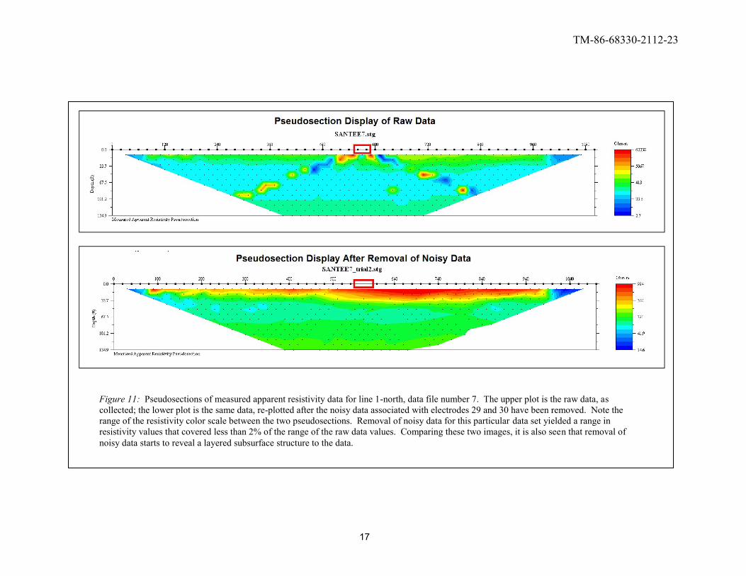
points from a file that shared a common electrode to be eliminated. Figure 11
shows two plots for data file number 7, line 1 north. Both plots in Figure 11 are
referred to as pseudosections. Pseudosections are a visual representation of
unprocessed apparent resistivity values. In this collected data file there were two
electrodes, numbers 29 and 30, which consistently measured noisy data. This
created resistivity artifacts in the pseudosection. The upper image is the raw data,
as collected, with very apparent noisy data. The lower image displays a
pseudosection of the data collected after removing the noisy data associated with
electrodes 29 and 30. Each data file was analyzed, and noisy data removed, prior
to data processing and interpretation.
TM-86-68330-2112-23
17
Figure 11: Pseudosections of measured apparent resistivity data for line 1-north, data file number 7. The upper plot is the raw data, as
collected; the lower plot is the same data, re-plotted after the noisy data associated with electrodes 29 and 30 have been removed. Note the
range of the resistivity color scale between the two pseudosections. Removal of noisy data for this particular data set yielded a range in
resistivity values that covered less than 2% of the range of the raw data values. Comparing these two images, it is also seen that removal of
noisy data starts to reveal a layered subsurface structure to the data.
TM-86-68330-2112-23
20
3.3 Data Processing and Interpretation There are two coupled techniques in geophysical data processing and
interpretation known as inversion and forward modeling. In order to perform one
process, the other process must also be performed. Therefore, the theoretical
basis of the two techniques is best understood when presented concurrently. Data
processing for the Santee Basin Aquifer Recharge Study involved the technique
of data inversion, and interpretation of the inversion results were aided by the use
of forward modeling. Both techniques aim to create an accurate model of a
physical property in the earth’s subsurface.
ERI data processing for this project consisted of performing two dimensional
inversions of the individually collected data files, usually 1100 feet in length.
Inversion is a mathematical process very common in geophysics by which
collected data of one parameter or more is used to formulate a model of the
physical parameter of interest. The collected data and the model parameter must
have some type of physical relation. In inverse and forward problems, there is a
mathematical relationship that links the measured quantities (data) to the
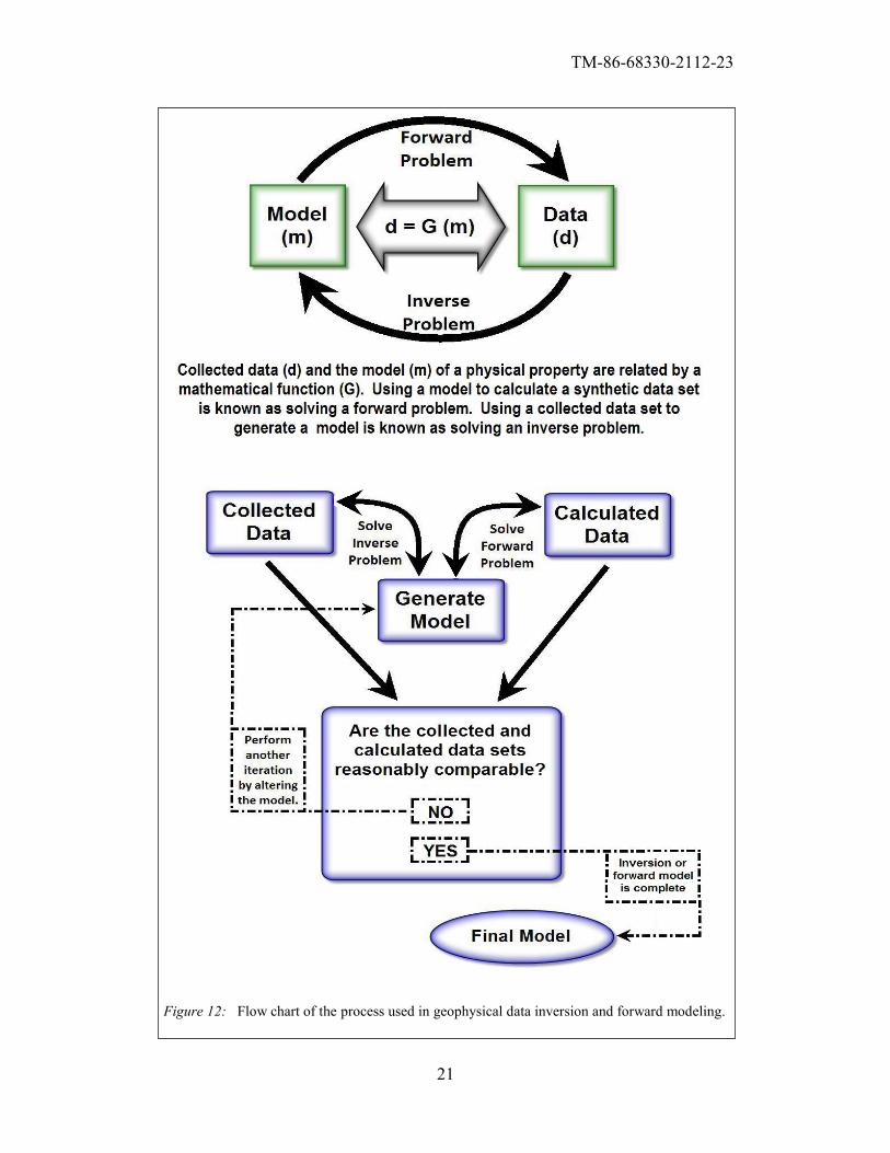
quantities of interest [5]. Figure 12 illustrates the relationship between data and
model, as well as forward modeling and inversion. In the inversion process a
generic model is generated, and through the forward modeling process a synthetic
data set is calculated. The collected and calculated data sets are compared for
equivalency. If the collected data and the calculated synthetic data sets do not
agree, the model is altered and another forward model is performed. Each time a
new synthetic data set is calculated and compared to a collected data set, it known
as an iteration of the inversion.
In the case of the ERI geophysical method, inversion of measured voltages creates
a model of earth resistivity. An important factor for the inversion of this data was
the manner in which the model was determined. These inversions used a finite
element model, which involved dividing the subsurface into cells, or blocks, and
determining the earth resistivity value of each cell [5]. The initial model for each
file inversion consisted of a homogeneous media with a resistivity value equal to
the average resistivity of all data points in the file. The initial models also begin
with the correct surface topography defined. The resistivity value of each cell in
the model was systematically adjusted until the model accurately reflected the
collected data. Each time the resistivity values of cells in the model are altered
and to the inversion of geophysical data is a computationally-intensive process,
involving numerous iterations and subsequent model adjustments. The specifics
of inversion theory are numerous and multi-faceted, and are discussed in detail in
the research literature for this topic [5].
TM-86-68330-2112-23
21
Figure 12: Flow chart of the process used in geophysical data inversion and forward modeling.
TM-86-68330-2112-23
22
Forward modeling is the theoretical inverse of the data inversion process, please
refer to Figure 12. The process can be utilized both prior to data collection and/or
after data inversion. For the Santee Basin Aquifer Recharge Study, the forward
modeling technique was used to aid in interpretation of collected ERI data. In
forward modeling, a subsurface model of the physical property of interest is
created. Based on that model, a synthetic data set is created with a defined
amount of random noise. That synthetic data set represents what would be the
expected data set from a geophysical survey conducted over a real earth structure
that mimics the created model. This synthetic data set may then go through the
data inversion process. The inversion resulting from the forward model can be
analyzed for survey planning, or compared to the inversion results from a
collected data set to aid in interpretation. Forward modeling is useful in both
survey planning and data interpretation as it allows for the effects that variations
in the subsurface will have on acquired data, and the resulting inversion of that
data. More information concerning specific forward modeling done for the
Santee Basin Aquifer Recharge Study is given in section 5.0.
Inversion and forward modeling of the data collected for the Santee Basin Aquifer
Recharge Study was done using commercially available software produced by the
manufacturers of the hardware used to collect the ERI data. Figures 13 and 14, on
the following pages, are examples of the output from the inversion (Figure 13)
and forward modeling (Figure 14) software. Throughout the rest of this TM,
inversion results and forward models will be presented in similar to format to
what is seen in Figures 13 and 14. The default graphical output from Earth
Imager™ always contains three plots in order to present the steps of the inversion
or forward modeling process. In most cases, all three Earth Imager™ plots are
presented. There are some instances in which individual plots from data
inversions and forward models are isolated and presented independently. In that
situation, please refer back to Figures 13 and 14 for clarification of plot axes,
color scales, figure annotations, etc.
TM-86-68330-2112-23
23
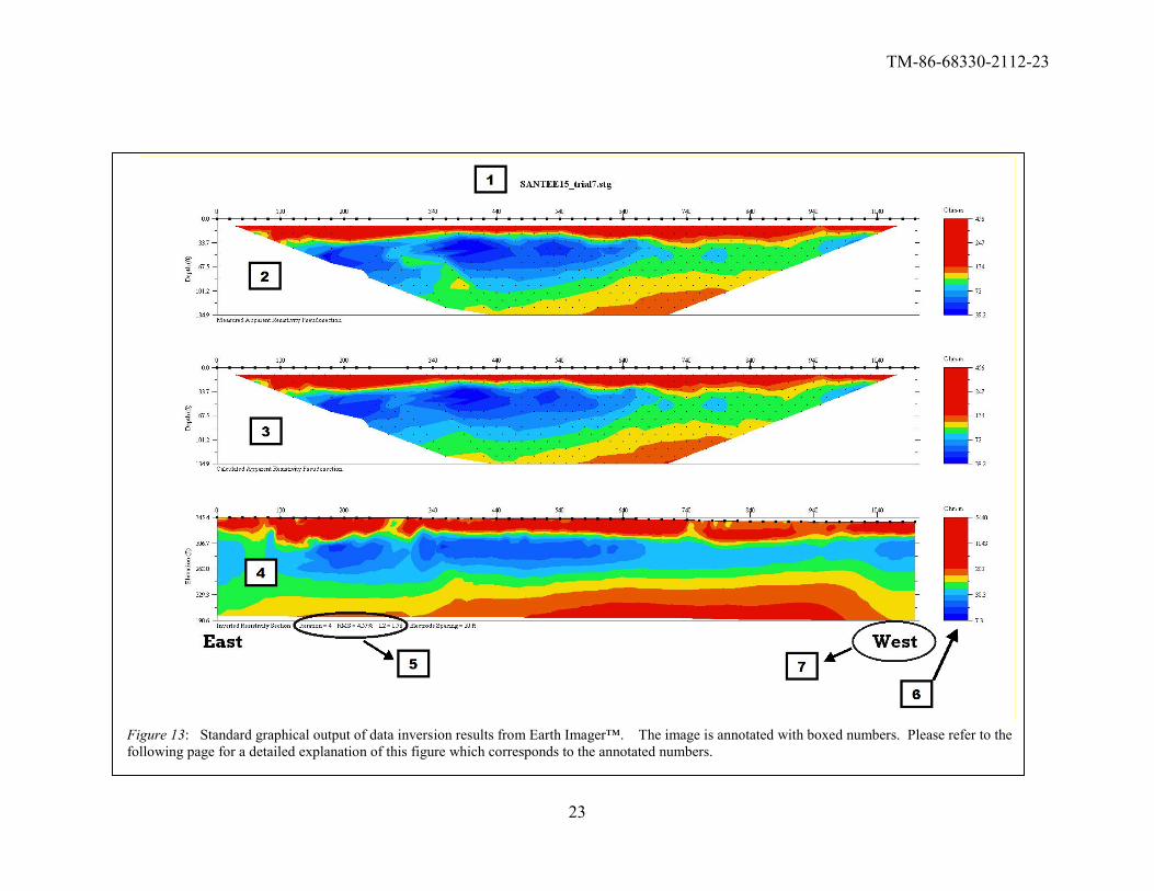
Figure 13: Standard graphical output of data inversion results from Earth Imager™. The image is annotated with boxed numbers. Please refer to the
following page for a detailed explanation of this figure which corresponds to the annotated numbers.
TM-86-68330-2112-23
24
Figure 13: Explanation of graphical standard output of inversion results from Earth Imager™.
1. Inversion titles for this project will always appear in this format:
SANTEE(data file number)_trial(number of times data set has been altered and saved).stg
2. Collected data set displayed as a pseudosection. Black dots are locations of individual data points. A color contour plot has been formatted for
the data set to display apparent resistivity values. The note at the lower left of this plot indicates it is a “Measured Apparent Resistivity
Pseudosection.” This note corresponds with a collected data. This plot is displayed with distance along the data file (in feet) for the horizontal
axis and depth (in feet) along the vertical axis.
3. Synthetic calculated data set displayed as a pseudosection. This plot presents the synthetic data set that is calculated from the final resulting
inversion. Black dots are locations of individual calculated data points. A color contour plot has been formatted for the data set to display
apparent resistivity values. The note at the lower left of this plot indicates it is a “Calculated Apparent Resistivity Pseudosection.” This note
corresponds with a synthetic calculated data set. This plot is displayed with distance along the data file (in feet) for the horizontal axis and depth
(in feet) along the vertical axis.
4. This plot is the final result of the inversion process. It is a model of subsurface electrical resistivity, and is the output from the inversion process
that is used for interpreting subsurface geologic structure. The note at the lower left of this plot indicates it is an “Inverted Resistivity Section.”
This note corresponds with a model of subsurface resistivity resulting from the inversion process. This plot is displayed with distance along the
data file (in feet) for the horizontal axis and elevation (in feet) along the vertical axis.
5. Inverted resistivity sections appear with calculation statistics listed below the plot. The iteration number refers to how many times the subsurface
was altered, a synthetic data set was calculated and the collected and calculated data sets were compared. The first iteration for all inversions done
for this project used a homogenous subsurface model with the resistivity equal to that of the average resistivity value of the data file. The RMS
stands for root mean square (in mathematics it is also known as the quadratic mean). The root mean square is a statistical measure of a varying
quantity. The RMS is calculated between the calculated data and the collected data and listed here. The lower the RMS percentage, the greater
equivalence there is between the collected and calculated data sets. The L2 number listed here is another measure of data misfit based on the
normalization of a least squares regression of the calculated data. When the L2 value is equal to, or less than 1.0, the inversion has converged,
meaning that the collected and calculated data sets are reasonable equivalent.
6. Each plot has its own color scale of resistivity values. Plots that occur in the same inversion figure will often have equal color scales for the
measured and calculated apparent resistivity pseudosections and a differing color scale for the inverted resistivity section. The color scales for this
project are all logarithmic, which yields greater color variation for more conductive values (cooler colors) and less color variation for highly
resistive values (warmer colors). All resistivity and apparent resistivity color scales are presented in ohm-meters, the SI unit for electrical
resistivity.
7. Inversion of collected data files for this project have been annotated with cardinal directions, so that the orientation of the data file may be
determined with respect to the survey area.
TM-86-68330-2112-23
25
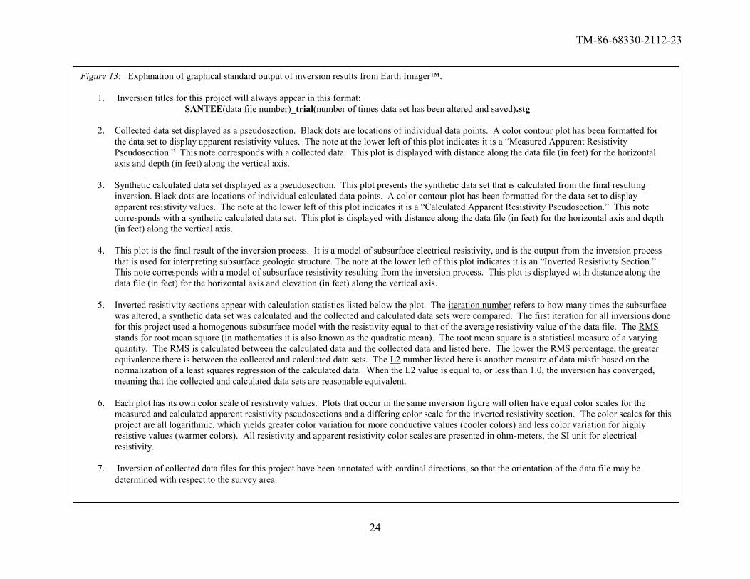
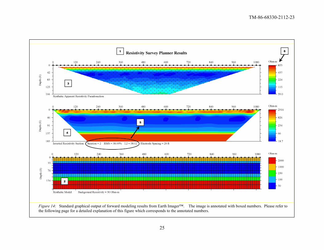
Figure 14: Standard graphical output of forward modeling results from Earth Imager™. The image is annotated with boxed numbers. Please refer to
the following page for a detailed explanation of this figure which corresponds to the annotated numbers.
TM-86-68330-2112-23
26
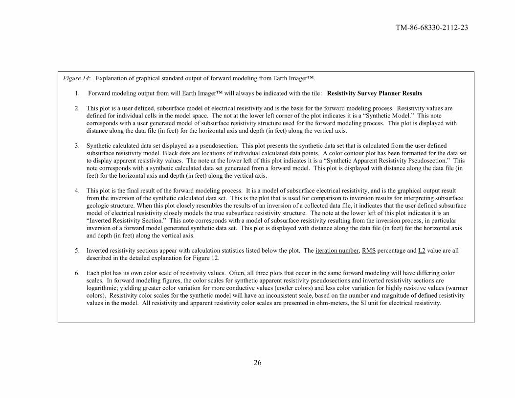
Figure 14: Explanation of graphical standard output of forward modeling from Earth Imager™.
1. Forward modeling output from will Earth Imager™ will always be indicated with the tile: Resistivity Survey Planner Results
2. This plot is a user defined, subsurface model of electrical resistivity and is the basis for the forward modeling process. Resistivity values are
defined for individual cells in the model space. The not at the lower left corner of the plot indicates it is a “Synthetic Model.” This note
corresponds with a user generated model of subsurface resistivity structure used for the forward modeling process. This plot is displayed with
distance along the data file (in feet) for the horizontal axis and depth (in feet) along the vertical axis.
3. Synthetic calculated data set displayed as a pseudosection. This plot presents the synthetic data set that is calculated from the user defined
subsurface resistivity model. Black dots are locations of individual calculated data points. A color contour plot has been formatted for the data set
to display apparent resistivity values. The note at the lower left of this plot indicates it is a “Synthetic Apparent Resistivity Pseudosection.” This
note corresponds with a synthetic calculated data set generated from a forward model. This plot is displayed with distance along the data file (in
feet) for the horizontal axis and depth (in feet) along the vertical axis.
4. This plot is the final result of the forward modeling process. It is a model of subsurface electrical resistivity, and is the graphical output result
from the inversion of the synthetic calculated data set. This is the plot that is used for comparison to inversion results for interpreting subsurface
geologic structure. When this plot closely resembles the results of an inversion of a collected data file, it indicates that the user defined subsurface
model of electrical resistivity closely models the true subsurface resistivity structure. The note at the lower left of this plot indicates it is an
“Inverted Resistivity Section.” This note corresponds with a model of subsurface resistivity resulting from the inversion process, in particular
inversion of a forward model generated synthetic data set. This plot is displayed with distance along the data file (in feet) for the horizontal axis
and depth (in feet) along the vertical axis.
5. Inverted resistivity sections appear with calculation statistics listed below the plot. The iteration number, RMS percentage and L2 value are all
described in the detailed explanation for Figure 12.
6. Each plot has its own color scale of resistivity values. Often, all three plots that occur in the same forward modeling will have differing color
scales. In forward modeling figures, the color scales for synthetic apparent resistivity pseudosections and inverted resistivity sections are
logarithmic; yielding greater color variation for more conductive values (cooler colors) and less color variation for highly resistive values (warmer
colors). Resistivity color scales for the synthetic model will have an inconsistent scale, based on the number and magnitude of defined resistivity
values in the model. All resistivity and apparent resistivity color scales are presented in ohm-meters, the SI unit for electrical resistivity.
TM-86-68330-2112-23
27
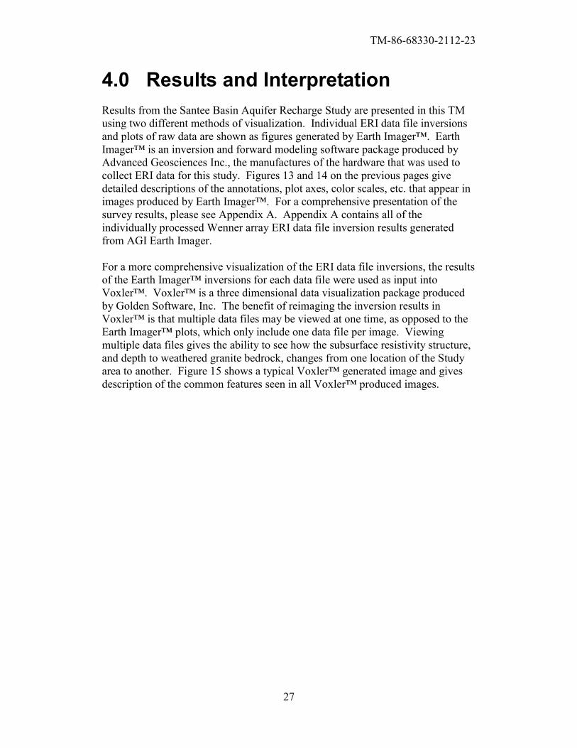
4.0 Results and Interpretation
Results from the Santee Basin Aquifer Recharge Study are presented in this TM
using two different methods of visualization. Individual ERI data file inversions
and plots of raw data are shown as figures generated by Earth Imager™. Earth
Imager™ is an inversion and forward modeling software package produced by
Advanced Geosciences Inc., the manufactures of the hardware that was used to
collect ERI data for this study. Figures 13 and 14 on the previous pages give
detailed descriptions of the annotations, plot axes, color scales, etc. that appear in
images produced by Earth Imager™. For a comprehensive presentation of the
survey results, please see Appendix A. Appendix A contains all of the
individually processed Wenner array ERI data file inversion results generated
from AGI Earth Imager.
For a more comprehensive visualization of the ERI data file inversions, the results
of the Earth Imager™ inversions for each data file were used as input into
Voxler™. Voxler™ is a three dimensional data visualization package produced
by Golden Software, Inc. The benefit of reimaging the inversion results in
Voxler™ is that multiple data files may be viewed at one time, as opposed to the
Earth Imager™ plots, which only include one data file per image. Viewing
multiple data files gives the ability to see how the subsurface resistivity structure,
and depth to weathered granite bedrock, changes from one location of the Study
area to another. Figure 15 shows a typical Voxler™ generated image and gives
description of the common features seen in all Voxler™ produced images.
TM-86-68330-2112-23
28
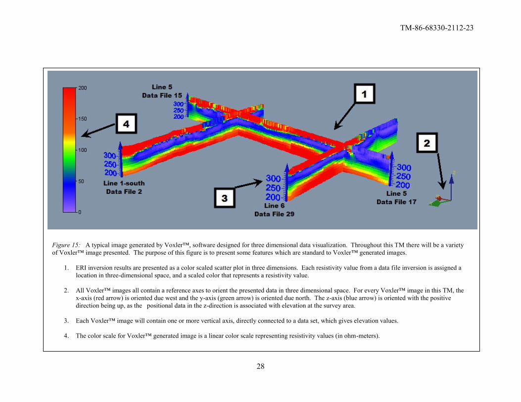
Figure 15: A typical image generated by Voxler™, software designed for three dimensional data visualization. Throughout this TM there will be a variety
of Voxler™ image presented. The purpose of this figure is to present some features which are standard to Voxler™ generated images.
1. ERI inversion results are presented as a color scaled scatter plot in three dimensions. Each resistivity value from a data file inversion is assigned a
location in three-dimensional space, and a scaled color that represents a resistivity value.
2. All Voxler™ images all contain a reference axes to orient the presented data in three dimensional space. For every Voxler™ image in this TM, the
x-axis (red arrow) is oriented due west and the y-axis (green arrow) is oriented due north. The z-axis (blue arrow) is oriented with the positive
direction being up, as the positional data in the z-direction is associated with elevation at the survey area.
3. Each Voxler™ image will contain one or more vertical axis, directly connected to a data set, which gives elevation values.
4. The color scale for Voxler™ generated image is a linear color scale representing resistivity values (in ohm-meters).
TM-86-68330-2112-23
29
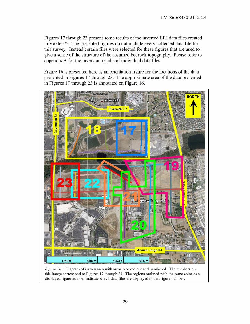
Figures 17 through 23 present some results of the inverted ERI data files created
in Voxler™. The presented figures do not include every collected data file for
this survey. Instead certain files were selected for these figures that are used to
give a sense of the structure of the assumed bedrock topography. Please refer to
appendix A for the inversion results of individual data files.
Figure 16 is presented here as an orientation figure for the locations of the data
presented in Figures 17 through 23. The approximate area of the data presented
in Figures 17 through 23 is annotated on Figure 16.
Figure 16: Diagram of survey area with areas blocked out and numbered. The numbers on
this image correspond to Figures 17 through 23. The regions outlined with the same color as a
displayed figure number indicate which data files are displayed in that figure number.
TM-86-68330-2112-23
30
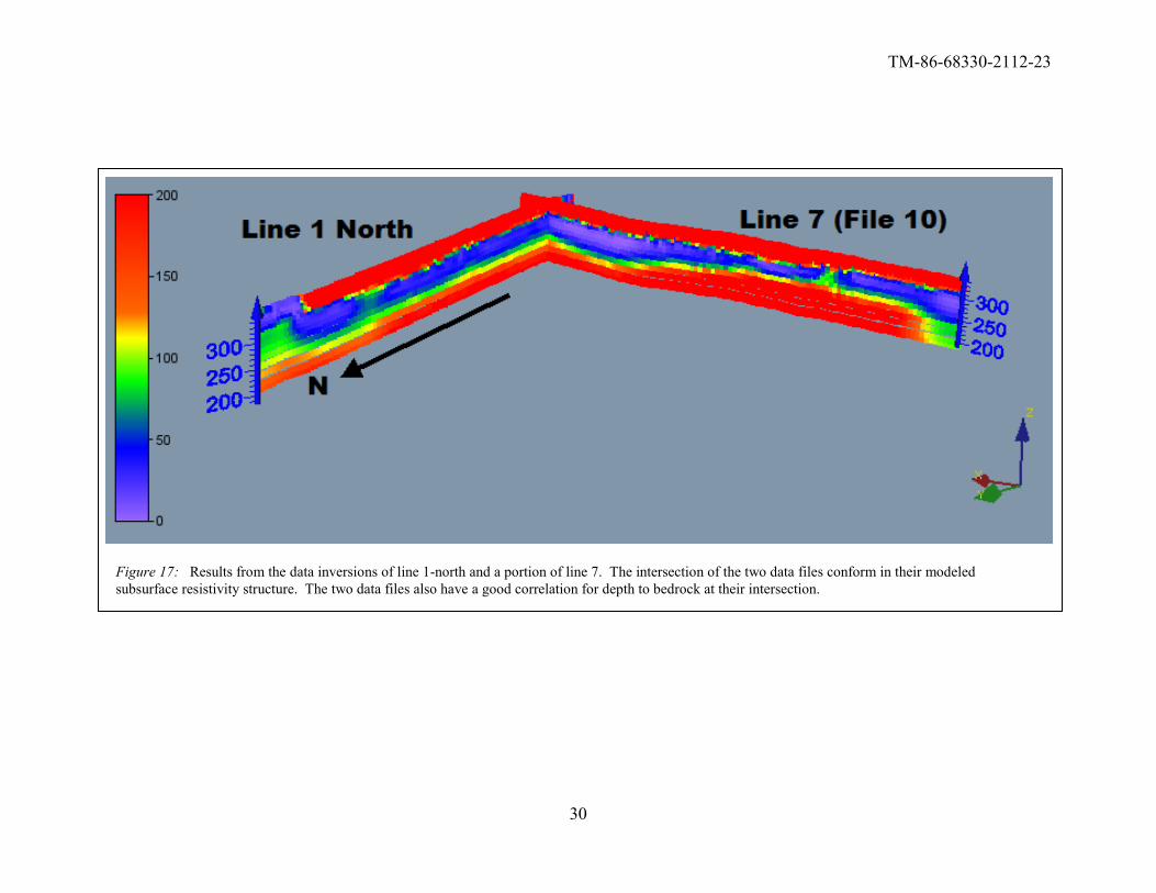
Figure 17: Results from the data inversions of line 1-north and a portion of line 7. The intersection of the two data files conform in their modeled
subsurface resistivity structure. The two data files also have a good correlation for depth to bedrock at their intersection.
TM-86-68330-2112-23
31
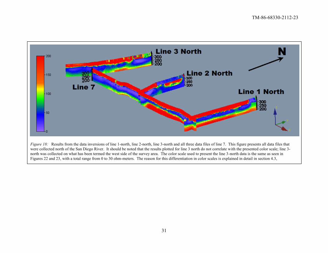
Figure 18: Results from the data inversions of line 1-north, line 2-north, line 3-north and all three data files of line 7. This figure presents all data files that
were collected north of the San Diego River. It should be noted that the results plotted for line 3 north do not correlate with the presented color scale; line 3-
north was collected on what has been termed the west side of the survey area. The color scale used to present the line 3-north data is the same as seen in
Figures 22 and 23, with a total range from 0 to 30 ohm-meters. The reason for this differentiation in color scales is explained in detail in section 4.3,
TM-86-68330-2112-23
32
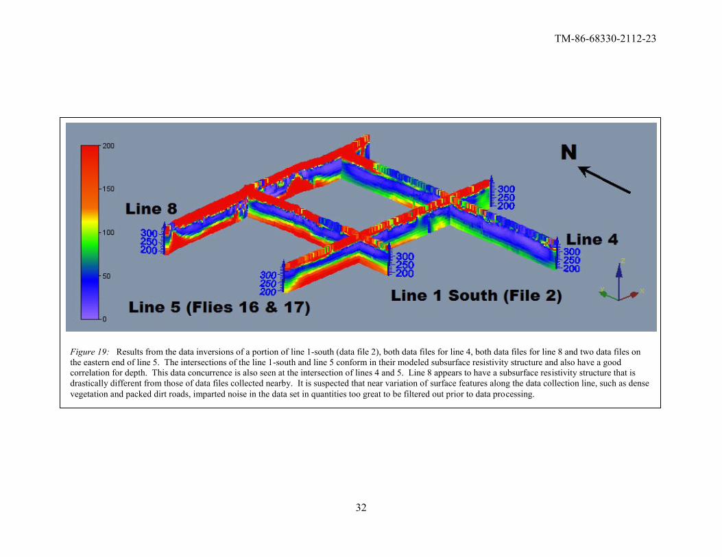
Figure 19: Results from the data inversions of a portion of line 1-south (data file 2), both data files for line 4, both data files for line 8 and two data files on
the eastern end of line 5. The intersections of the line 1-south and line 5 conform in their modeled subsurface resistivity structure and also have a good
correlation for depth. This data concurrence is also seen at the intersection of lines 4 and 5. Line 8 appears to have a subsurface resistivity structure that is
drastically different from those of data files collected nearby. It is suspected that near variation of surface features along the data collection line, such as dense
vegetation and packed dirt roads, imparted noise in the data set in quantities too great to be filtered out prior to data processing.
TM-86-68330-2112-23
33
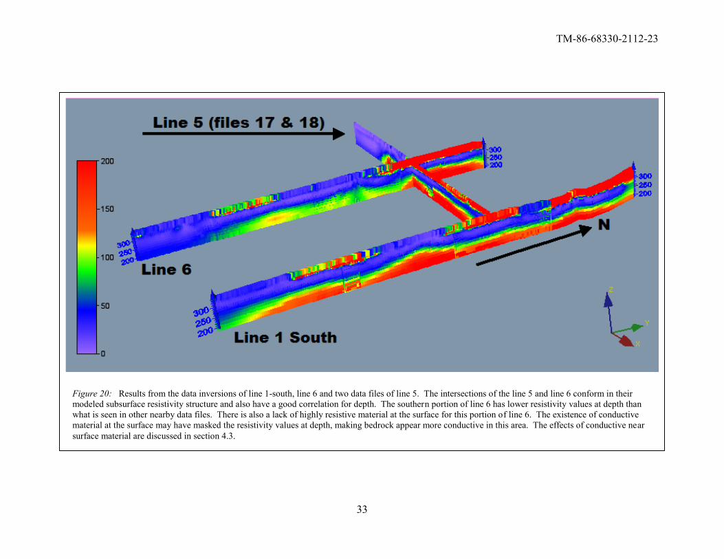
Figure 20: Results from the data inversions of line 1-south, line 6 and two data files of line 5. The intersections of the line 5 and line 6 conform in their
modeled subsurface resistivity structure and also have a good correlation for depth. The southern portion of line 6 has lower resistivity values at depth than
what is seen in other nearby data files. There is also a lack of highly resistive material at the surface for this portion of line 6. The existence of conductive
material at the surface may have masked the resistivity values at depth, making bedrock appear more conductive in this area. The effects of conductive near
surface material are discussed in section 4.3.
TM-86-68330-2112-23
34
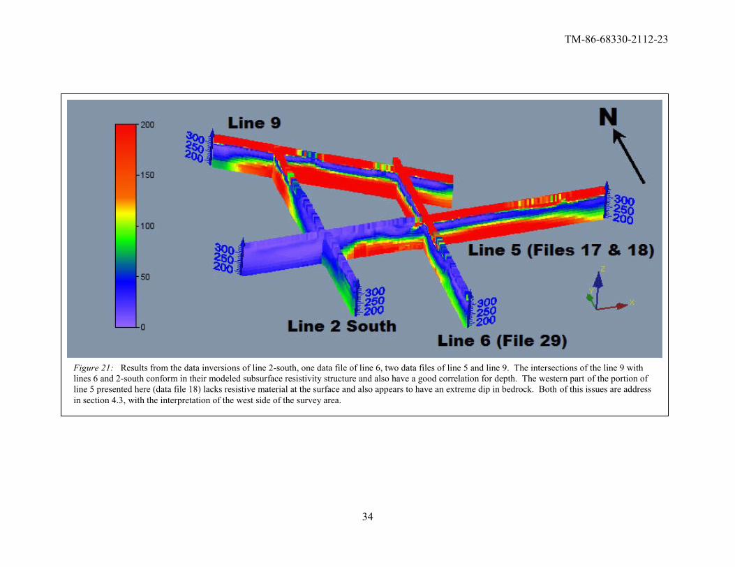
Figure 21: Results from the data inversions of line 2-south, one data file of line 6, two data files of line 5 and line 9. The intersections of the line 9 with
lines 6 and 2-south conform in their modeled subsurface resistivity structure and also have a good correlation for depth. The western part of the portion of
line 5 presented here (data file 18) lacks resistive material at the surface and also appears to have an extreme dip in bedrock. Both of this issues are address
in section 4.3, with the interpretation of the west side of the survey area.
TM-86-68330-2112-23
35
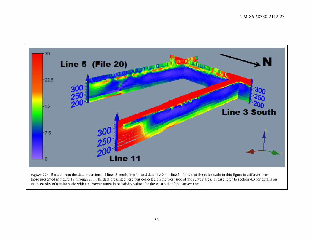
Figure 22: Results from the data inversions of lines 3-south, line 11 and data file 20 of line 5. Note that the color scale in this figure is different than
those presented in figure 17 through 21. The data presented here was collected on the west side of the survey area. Please refer to section 4.3 for details on
the necessity of a color scale with a narrower range in resistivity values for the west side of the survey area.
TM-86-68330-2112-23
36
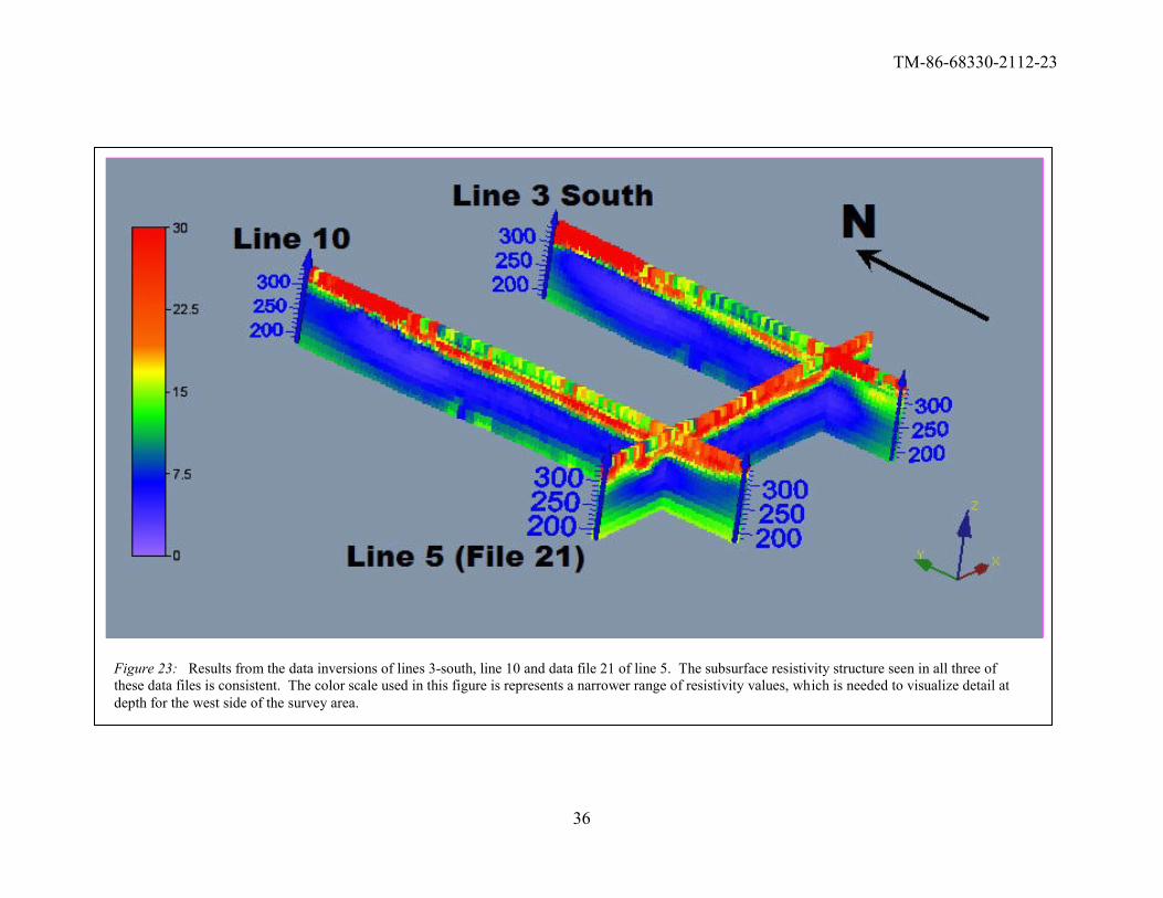
Figure 23: Results from the data inversions of lines 3-south, line 10 and data file 21 of line 5. The subsurface resistivity structure seen in all three of
these data files is consistent. The color scale used in this figure is represents a narrower range of resistivity values, which is needed to visualize detail at
depth for the west side of the survey area.
TM-86-68330-2112-23
37
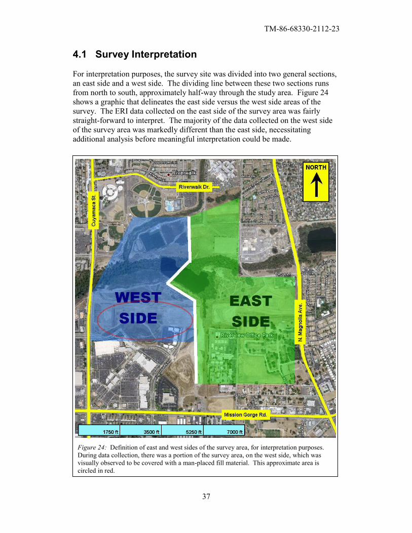
4.1 Survey Interpretation
For interpretation purposes, the survey site was divided into two general sections,
an east side and a west side. The dividing line between these two sections runs
from north to south, approximately half-way through the study area. Figure 24
shows a graphic that delineates the east side versus the west side areas of the
survey. The ERI data collected on the east side of the survey area was fairly
straight-forward to interpret. The majority of the data collected on the west side
of the survey area was markedly different than the east side, necessitating
additional analysis before meaningful interpretation could be made.
Figure 24: Definition of east and west sides of the survey area, for interpretation purposes.
During data collection, there was a portion of the survey area, on the west side, which was
visually observed to be covered with a man-placed fill material. This approximate area is
circled in red.
TM-86-68330-2112-23
38
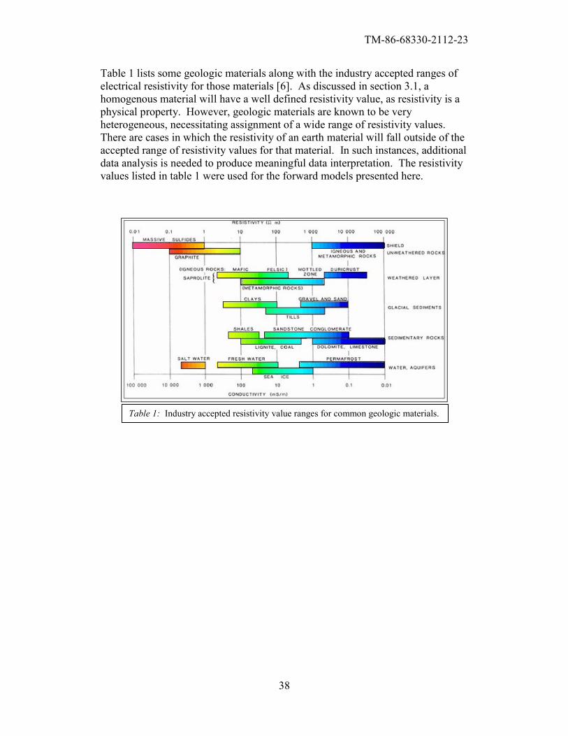
Table 1 lists some geologic materials along with the industry accepted ranges of
electrical resistivity for those materials [6]. As discussed in section 3.1, a
homogenous material will have a well defined resistivity value, as resistivity is a
physical property. However, geologic materials are known to be very
heterogeneous, necessitating assignment of a wide range of resistivity values.
There are cases in which the resistivity of an earth material will fall outside of the
accepted range of resistivity values for that material. In such instances, additional
data analysis is needed to produce meaningful data interpretation. The resistivity
values listed in table 1 were used for the forward models presented here.
Table 1: Industry accepted resistivity value ranges for common geologic materials.
TM-86-68330-2112-23
39
4.2 East Side Interpretation
Data collection on the east side of the survey site tended to be in areas covered by
sediments that appeared to be minimally altered from their natural depositional
environment. This produced inversion results which were interpreted as being
close to true earth resistivity values. The inversion results from the east side
produced subsurface models with resistivity values that fell within the range of
industry accepted resistivity values for the interpreted geologic materials.
For interpretation of the ERI inversion results, forward modeling was done using
AGI Earth Imager. The east side of the survey was generally interpreted as
consisting of three layer geologic model. This model consisted of near surface,
unsaturated alluvial sediments, underlain by sediments of similar composition, yet
completely saturated, and bounded at the bottom by the granitic bedrock structure
known to exist in the area. Figure 25 presents the resulting forward model for this
geologic structure. Please refer to Figure 13, in section 3.3, for display details of
forward modeling plots.
TM-86-68330-2112-23
40
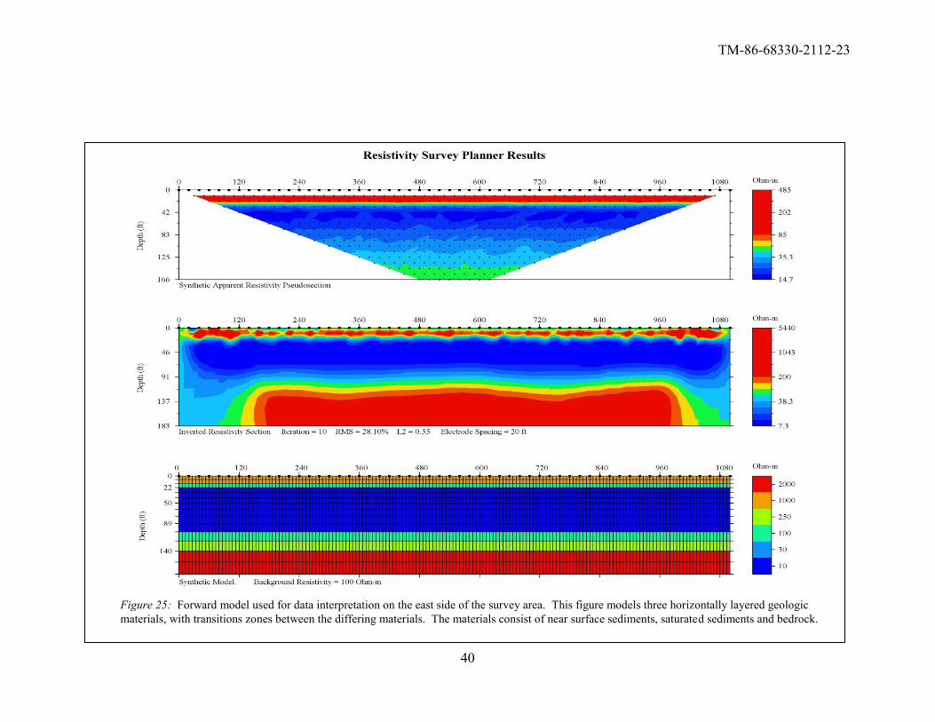
Figure 25: Forward model used for data interpretation on the east side of the survey area. This figure models three horizontally layered geologic
materials, with transitions zones between the differing materials. The materials consist of near surface sediments, saturated sediments and bedrock.
TM-86-68330-2112-23
41
The geologic model, the resulting synthetic data set and the forward model
inversion that is used for interpretation of the east side of the survey area is
presented in Figure 25. The uppermost 15 feet are modeled using a resistivity of
1000 ohm-meters; this layer is used to represent unsaturated alluvial sediments.
The resistivity value of 1000 ohm-meters lies towards higher end of the range of
industry accepted values of unsaturated, sandy sediments. A thin transition layer
was modeled between the upper unsaturated sediments and the top of the water
table. This thin layer is used to represent the vadose zone, and is modeled from
15 to 22 feet in depth, at 100 ohm-meters. The saturated sediments within the
water table are modeled with a resistivity value of 10 ohm-meters, this value lies
at the conductive end of industry accepted range of resistivity values for fresh
water aquifers. Below the saturated sediments in the water table there is a gradual
transition in resistivity values from the more conductive water table into the more
resistive bedrock. This transition zone is modeled with two layers; the top layer
has a resistivity of 100 ohm-meters, and occurs from roughly 100 to 120 feet in
depth. Below that, a layer from roughly 120 to 140 feet in depth is modeled at
250 ohm-meters. This transition zone is included in order to more accurately
model the subsurface conditions noted on drill logs from area wells. Bedrock is
described as weathered granitic boulders and cobbles at its uppermost extent, and
transitioning into a more competent granitic structure with depth. Weathered
granite will have a lower resistivity value than that of competent granite due to a
combination of factors. The increased fracturing encountered in weathered
granite allows for penetration of ground water. Additionally, granite decomposes
into clay-rich sediments, which are more electrically conductive than sandy
sediments. Below the saturated, weathered granite transition zone is the modeled
bedrock layer. The competent granitic bedrock layer is modeled with a resistivity
of 2000 ohm-meters with its upper extent occurring at a depth of approximately
140 feet.
The synthetic data set generated from the model included the addition of 5%
random noise. The pseudosection of the synthetic data generated from the
geologic model is included in the top plot of Figure 25. The center plot of Figure
25 is the resulting inversion of the forward model generated synthetic data. To
demonstrate the validity of the geologic model used for the east side of the survey
area the inversion results from several data files collected on the east side are
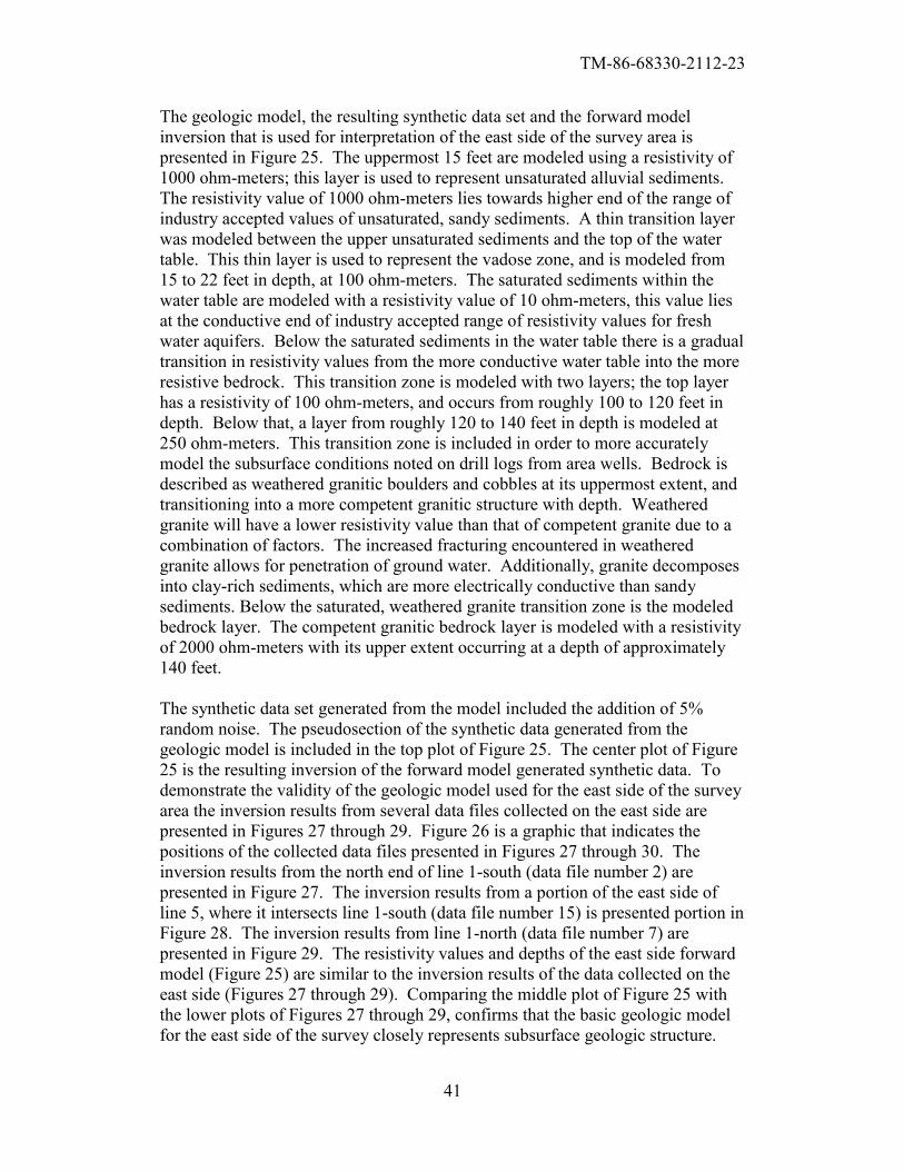
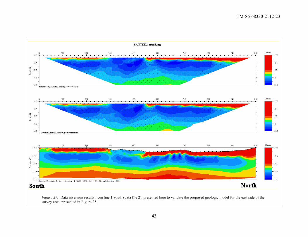
presented in Figures 27 through 29. Figure 26 is a graphic that indicates the
positions of the collected data files presented in Figures 27 through 30. The
inversion results from the north end of line 1-south (data file number 2) are
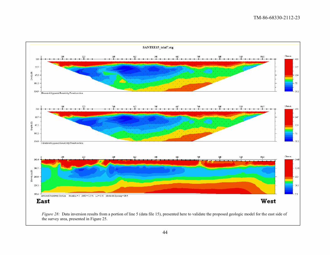
presented in Figure 27. The inversion results from a portion of the east side of
line 5, where it intersects line 1-south (data file number 15) is presented portion in
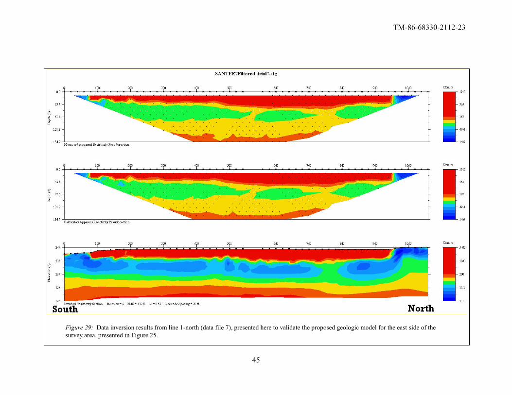
Figure 28. The inversion results from line 1-north (data file number 7) are
presented in Figure 29. The resistivity values and depths of the east side forward
model (Figure 25) are similar to the inversion results of the data collected on the
east side (Figures 27 through 29). Comparing the middle plot of Figure 25 with
the lower plots of Figures 27 through 29, confirms that the basic geologic model
for the east side of the survey closely represents subsurface geologic structure.
TM-86-68330-2112-23
42
Figure 26: Location map of data presented in Figures 27 through 29. The
inversion results from these data files confirm the subsurface resistivity
structure proposed for the east side of the survey area, as presented in the
forward model from Figure 25.
TM-86-68330-2112-23
43
Figure 27: Data inversion results from line 1-south (data file 2), presented here to validate the proposed geologic model for the east side of the
survey area, presented in Figure 25.
TM-86-68330-2112-23
44
Figure 28: Data inversion results from a portion of line 5 (data file 15), presented here to validate the proposed geologic model for the east side of
the survey area, presented in Figure 25.
TM-86-68330-2112-23
45
Figure 29: Data inversion results from line 1-north (data file 7), presented here to validate the proposed geologic model for the east side of the
survey area, presented in Figure 25.
TM-86-68330-2112-23
46
4.3 West Side Interpretation
Data collection on the west side of the survey site tended to occur over near
surface sediments that appeared directly man-placed, and thus not in their natural
geologic depositional environments. Of particular interest on the west side of the
survey area was the placed fill to the north of the shopping and office
developments at the corner of Cuyamaca Street and Mission Gorge Road. This
area is encircled with a red oval in Figure 24.
The initial ERI data inversion results on the west side of the survey area are all
much more electrically conductive than the inversion results from the data
collected on the east side of the survey area. The highest resistivity value
observed in a data file that was collected on the west side of the survey was often
less than 100 ohm-meters. This is at least an order of magnitude less than the
high resistivity values collected on the east side of the survey area, where the
highest resistivity within a data set is often greater than 1000 ohm-meters. The
most apparent reason for this variation in subsurface resistivity values was
attributed to a man-placed fill material observed on site. During data collection, it
was noted that data files collected over this man-placed fill contained a much
narrower range in resistivity values, with the highest collected resistivity values
being comparable to the lower resistivity values seen on the east side of the
survey area.
The initial ERI data inversion results on the west side of the survey area appeared
to have a greater depth to the top of bedrock than what was seen on the east side
of the survey area. This variation in depth to bedrock from the east side to the
west side could be attributed to either the resistivity masking from the highly
conductive overburden or to an actual trend in the bedrock surface topography, or
a combination of both of these factors.
For interpretation of the data collected over the observed, highly conductive fill
material and apparent increase in depth to bedrock, a different subsurface
geologic model was created. This model was generated on the assumption that
the man-placed conductive fill material was directly overlying the assumed three
layer model used for interpretation of data collected in the east side of the survey
area. This assumption lead to the generation of a forward model that could
account for the effects this man-placed fill would have on the collection of ERI
data. This assumption was verified by using a forward model that includes a layer
of highly conductive fill on top of what is basically the same geologic model used
on the east side. An increased depth to bedrock was also accounted for in the
forward model for the west side of the survey area. Figure 30 presents the
geologic structure that was used as the basis for data interpretation on the west
side of the survey area. Figure 30 also presents the resulting synthetic data set
from said model, with 5% random noise added, and the inversion results of the
forward modeled data set. There are a few differences between the geologic
models in Figures 25 and 30. The most obvious difference is the upper 20 feet of
TM-86-68330-2112-23
47
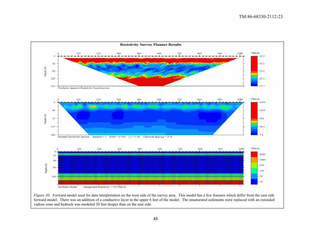
the model. A highly conductive (10 ohm-meter) layer was placed on the upper 6
feet of the model to account for the conductive man placed fill. The unsaturated
sediments from the east side geologic model were replaced with a 100 ohm-meter
layer (depths 6 to 15 feet). The removal of the unsaturated sediments was done
because the man-placed fill likely acts as an evaporative barrier for the water
table, this layer essentially extends the vadose zone close to the ground surface.
The final variation between the east side and west side forward models is the
depth at which decomposed granite is modeled. For the west side forward model
the transition zone layers start at 100 ohm-meter from depths 120 to 140 feet, and
a 250 ohm-meter layer from 140 to 160 feet in depth. Competent granite,
modeled at 2000 ohm-meters, begins at a depth of 160 feet; this is 20 feet deeper
than what was modeled on the east side of the survey area. Figure 30 was re-
plotted at a different color scale and re-represented as Figure 31. The rationale
behind re-scaling the plot is discussed further in this section.
TM-86-68330-2112-23
48
Figure 30: Forward model used for data interpretation on the west side of the survey area. This model has a few features which differ from the east side
forward model. There was an addition of a conductive layer in the upper 6 feet of the model. The unsaturated sediments were replaced with an extended
vadose zone and bedrock was modeled 20 feet deeper than on the east side.
TM-86-68330-2112-23
49
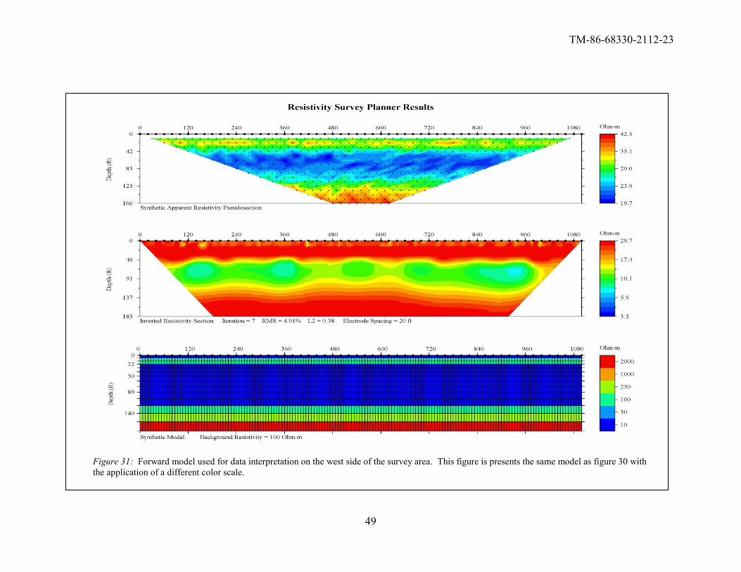
Figure 31: Forward model used for data interpretation on the west side of the survey area. This figure is presents the same model as figure 30 with
the application of a different color scale.
TM-86-68330-2112-23
50
Figure 30 utilizes the same color scale that was presented in Figures 25, and 27
through 29. This color scale ranges from a lower limit of 7.3 ohm-meters to an
upper limit of 5440 ohm-meters. The range of this color scale is much larger than
what is needed to display the data from the files that were collected over the man-
placed conductive fill material on the west side of the survey area. The results of
the forward model for the conductive fill over the basic three layer geologic
model were plotted again using a color scale with a much narrower range in
resistivity values. This re-scaled version of Figure 30 is presented in Figure 31.
Note that the color scale for Figure 31 ranges from a lower limit of 3.5 ohm-
meters to an upper limit of 29.3 ohm-meters. It should be noted that the created
geologic model, which is the basis for the forward model that accounts for the
effects of the conductive man-placed fill material and a greater depth to top of
bedrock, in Figures 30 and 31 are identical. Altering the color scale does not have
any effect on the created model. It also has no effect on the numerical values of
synthetic data set generated by the model or the resulting inversion of that
synthetic data. The purpose of re-scaling the color range is so that more detail can
be visually recovered in the resulting inversion of the forward model. Comparing
the middle plots of Figures 30 and 31, it can be seen that the color scale which
represents a narrower range in resistivity values yields visualization of the
inversion results which more closely reflect the suspected subsurface geologic
structure.
Much of the data collected on the west side of the survey area had a near surface,
conductive overburden that was not present on the east side of the survey.
Narrowing the range of resistivity values presented on the color scale for data
collected on the west side of the survey area allowed for the recovery of geologic
detail at depth. The presence of this conductive top layer had a masking affect on
the collected data, which made it difficult to determine true earth resistivity values
at depth. The physical result of this geologic model was that the conductive
overburden trapped the injected current so that less electrical current penetrated to
depth. This “current trapping” phenomena occurred when the current injection
electrodes were located in this man-placed fill material. Refer to Figure 2, in
section 2.1, case A, for an illustration of the concept that describes what occurs
with the injected electrical current on the west side of the survey area.
The inversion results of three of the data files collected directly over the
conductive man-placed fill, on the west side of the survey area, are presented in
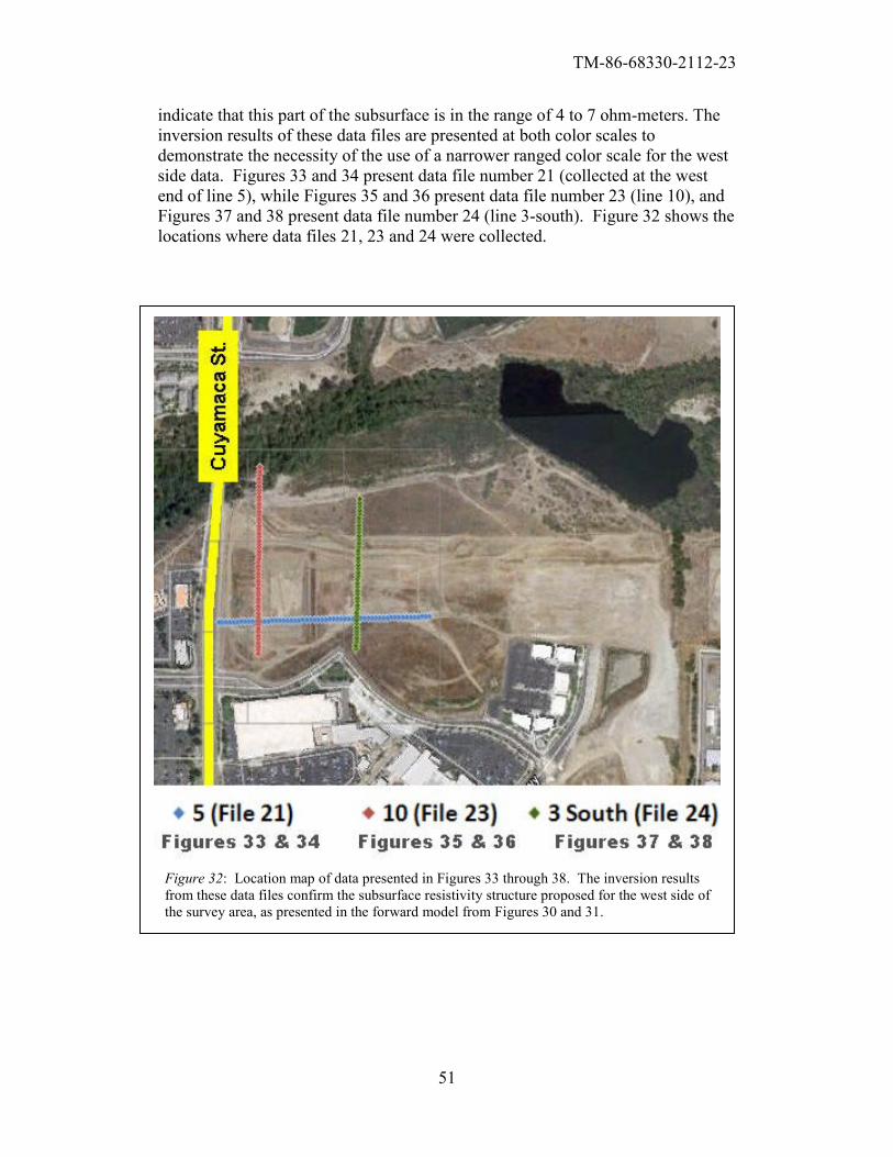
Figures 33 through 38; a location map for these figures is presented in Figure 32.
These figures are presented in order to demonstrate the validity of, and the effects
caused by, the geologic model that accounts for the conductive man-placed fill
that overburdens a larger portion of the west side of the survey area as well as an
increased depth to bedrock on the west side of the survey area. It should be noted
that the forward model presented in Figures 30 and 31 was not able to recover the
saturated sediments of the water table at values as conductive as the ERI data
inversions from the west side present. The forward model values the resistivity of
the water table in the 8 to 12 ohm-meter range and the ERI data inversion results
TM-86-68330-2112-23
51
indicate that this part of the subsurface is in the range of 4 to 7 ohm-meters. The
inversion results of these data files are presented at both color scales to
demonstrate the necessity of the use of a narrower ranged color scale for the west
side data. Figures 33 and 34 present data file number 21 (collected at the west
end of line 5), while Figures 35 and 36 present data file number 23 (line 10), and
Figures 37 and 38 present data file number 24 (line 3-south). Figure 32 shows the
locations where data files 21, 23 and 24 were collected.
Figure 32: Location map of data presented in Figures 33 through 38. The inversion results
from these data files confirm the subsurface resistivity structure proposed for the west side of
the survey area, as presented in the forward model from Figures 30 and 31.
TM-86-68330-2112-23
52
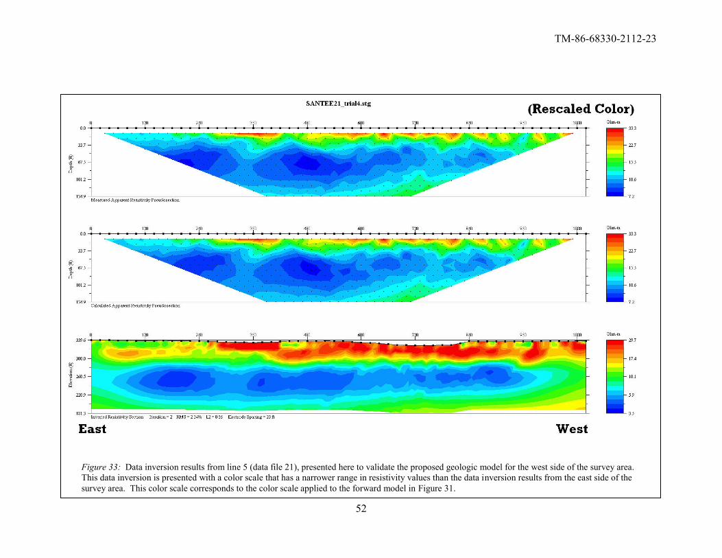
Figure 33: Data inversion results from line 5 (data file 21), presented here to validate the proposed geologic model for the west side of the survey area.
This data inversion is presented with a color scale that has a narrower range in resistivity values than the data inversion results from the east side of the
survey area. This color scale corresponds to the color scale applied to the forward model in Figure 31.
TM-86-68330-2112-23
53
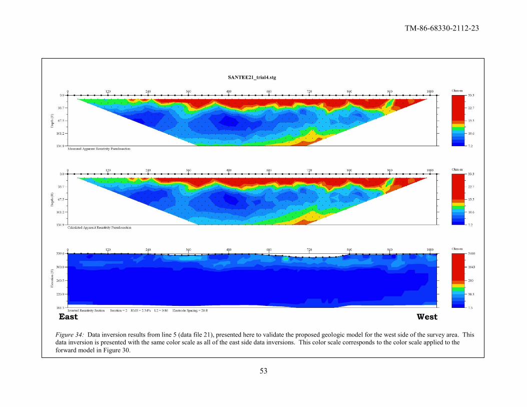
Figure 34: Data inversion results from line 5 (data file 21), presented here to validate the proposed geologic model for the west side of the survey area. This
data inversion is presented with the same color scale as all of the east side data inversions. This color scale corresponds to the color scale applied to the
forward model in Figure 30.
TM-86-68330-2112-23
54
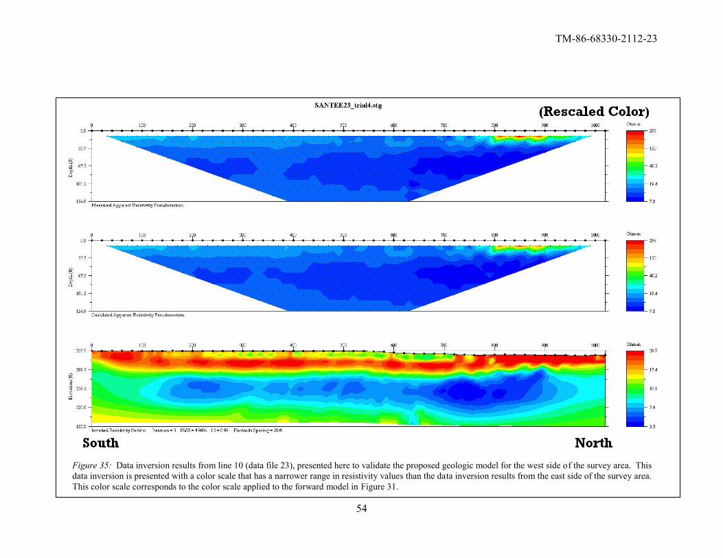
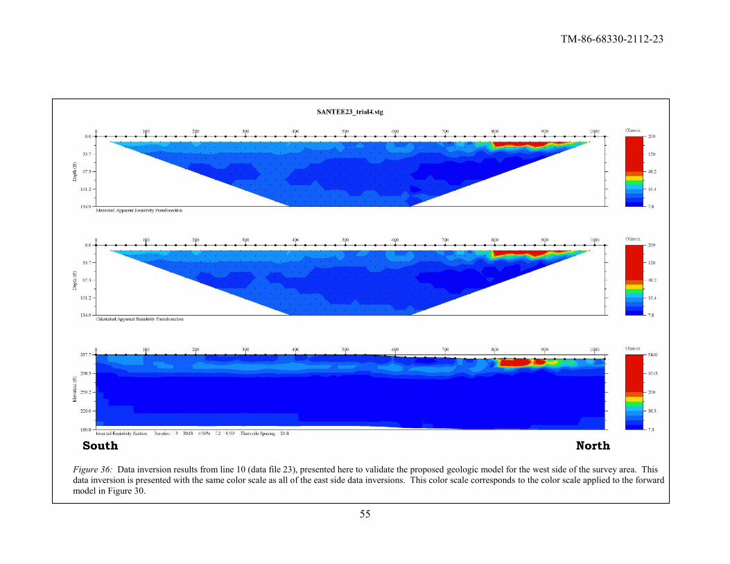
Figure 35: Data inversion results from line 10 (data file 23), presented here to validate the proposed geologic model for the west side of the survey area. This
data inversion is presented with a color scale that has a narrower range in resistivity values than the data inversion results from the east side of the survey area.
This color scale corresponds to the color scale applied to the forward model in Figure 31.
TM-86-68330-2112-23
55
Figure 36: Data inversion results from line 10 (data file 23), presented here to validate the proposed geologic model for the west side of the survey area. This
data inversion is presented with the same color scale as all of the east side data inversions. This color scale corresponds to the color scale applied to the forward
model in Figure 30.
TM-86-68330-2112-23
56
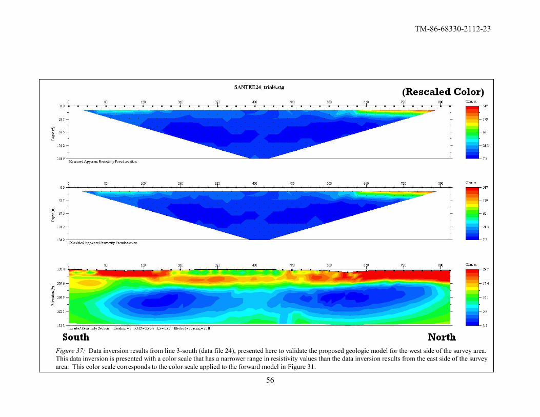
Figure 37: Data inversion results from line 3-south (data file 24), presented here to validate the proposed geologic model for the west side of the survey area.
This data inversion is presented with a color scale that has a narrower range in resistivity values than the data inversion results from the east side of the survey
area. This color scale corresponds to the color scale applied to the forward model in Figure 31.
TM-86-68330-2112-23
57
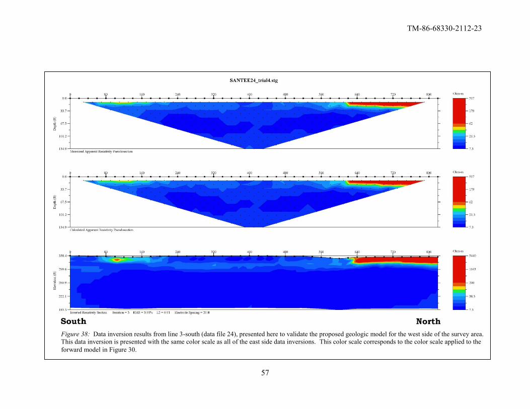
Figure 38: Data inversion results from line 3-south (data file 24), presented here to validate the proposed geologic model for the west side of the survey area.
This data inversion is presented with the same color scale as all of the east side data inversions. This color scale corresponds to the color scale applied to the
forward model in Figure 30.
TM-86-68330-2112-23
58
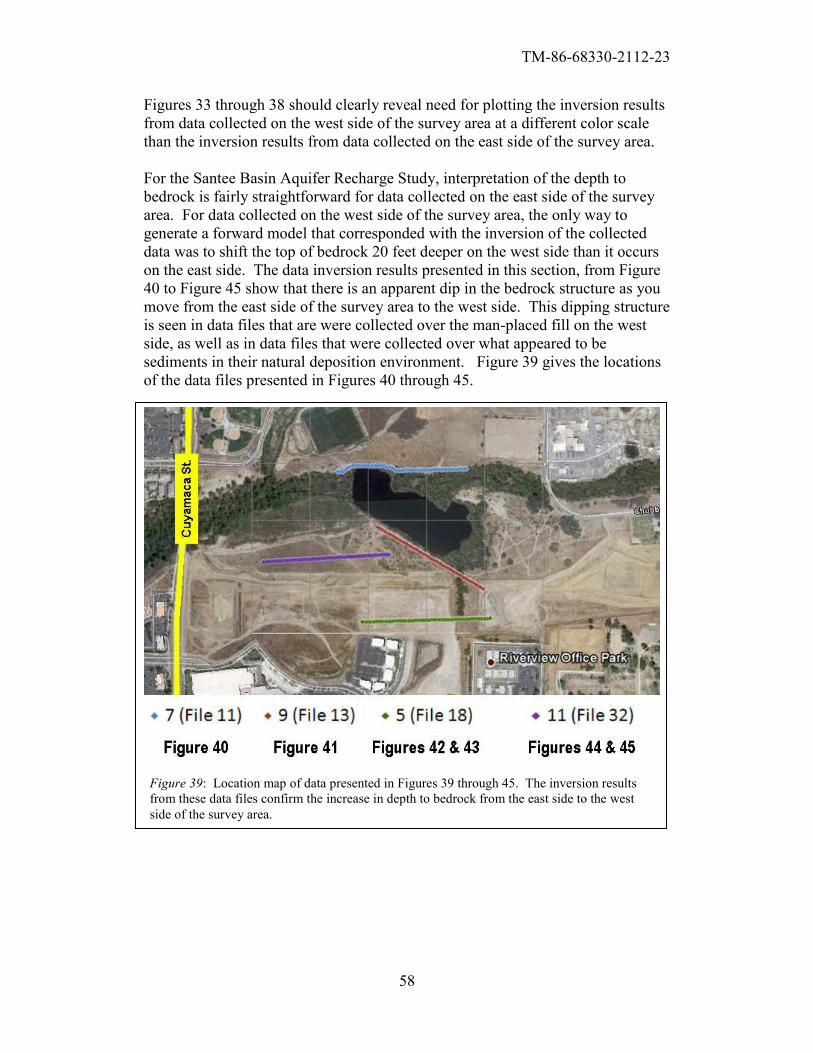
Figures 33 through 38 should clearly reveal need for plotting the inversion results
from data collected on the west side of the survey area at a different color scale
than the inversion results from data collected on the east side of the survey area.
For the Santee Basin Aquifer Recharge Study, interpretation of the depth to
bedrock is fairly straightforward for data collected on the east side of the survey
area. For data collected on the west side of the survey area, the only way to
generate a forward model that corresponded with the inversion of the collected
data was to shift the top of bedrock 20 feet deeper on the west side than it occurs
on the east side. The data inversion results presented in this section, from Figure
40 to Figure 45 show that there is an apparent dip in the bedrock structure as you
move from the east side of the survey area to the west side. This dipping structure
is seen in data files that are were collected over the man-placed fill on the west
side, as well as in data files that were collected over what appeared to be
sediments in their natural deposition environment. Figure 39 gives the locations
of the data files presented in Figures 40 through 45.
FIGURE 39 – location map
Figure 39: Location map of data presented in Figures 39 through 45. The inversion results
from these data files confirm the increase in depth to bedrock from the east side to the west
side of the survey area.
TM-86-68330-2112-23
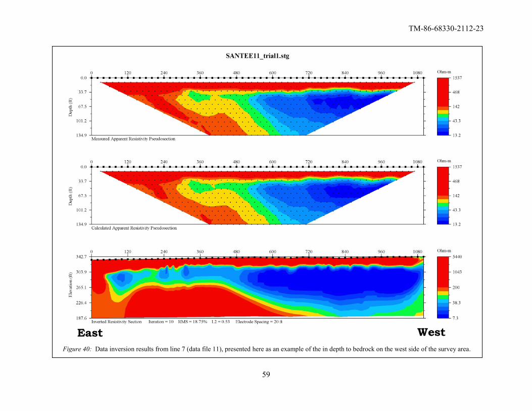
59
Figure 40: Data inversion results from line 7 (data file 11), presented here as an example of the in depth to bedrock on the west side of the survey area.
TM-86-68330-2112-23
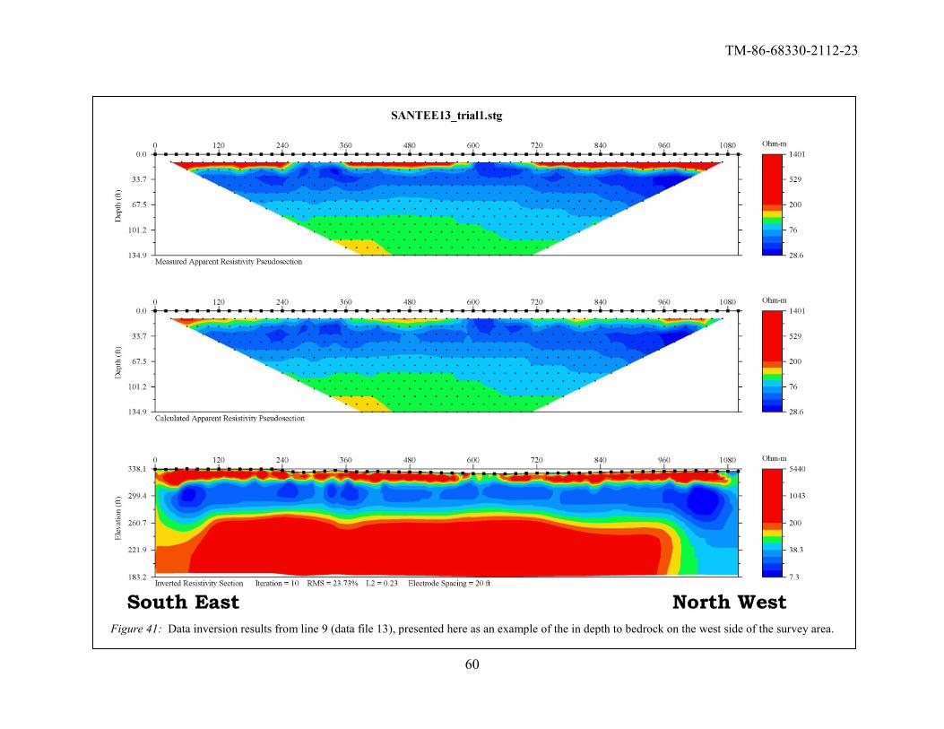
60
Figure 41: Data inversion results from line 9 (data file 13), presented here as an example of the in depth to bedrock on the west side of the survey area.
TM-86-68330-2112-23
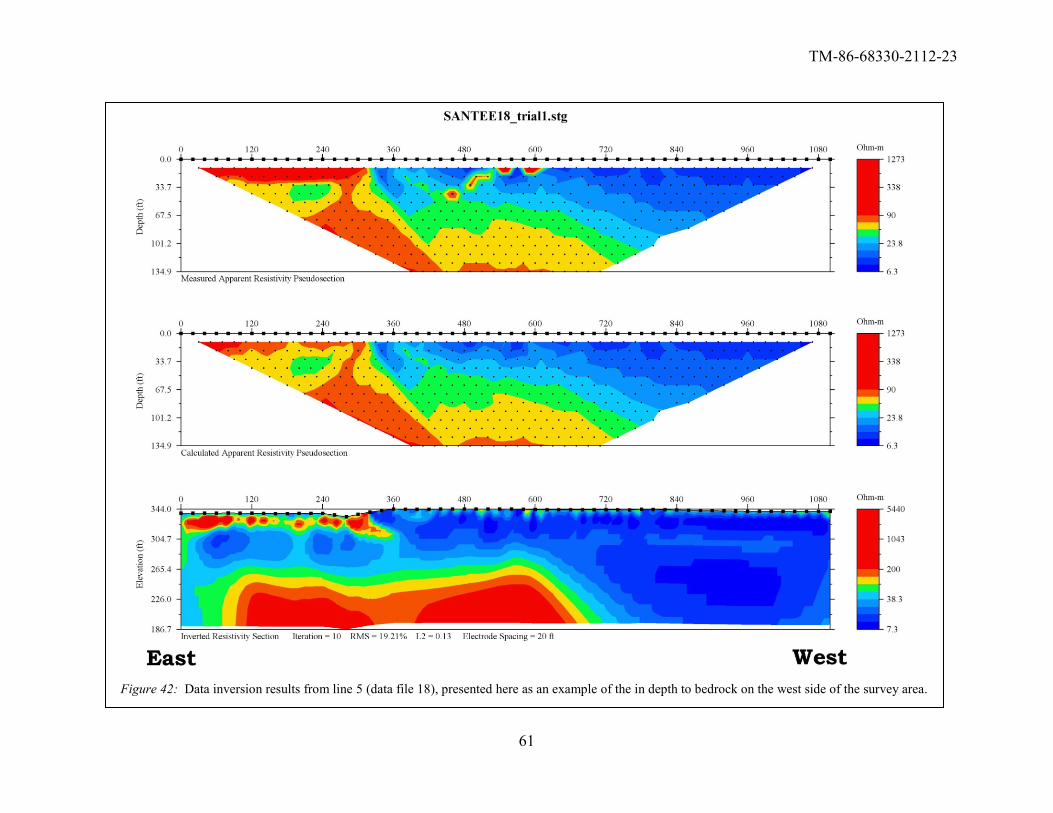
61
Figure 42: Data inversion results from line 5 (data file 18), presented here as an example of the in depth to bedrock on the west side of the survey area.
TM-86-68330-2112-23
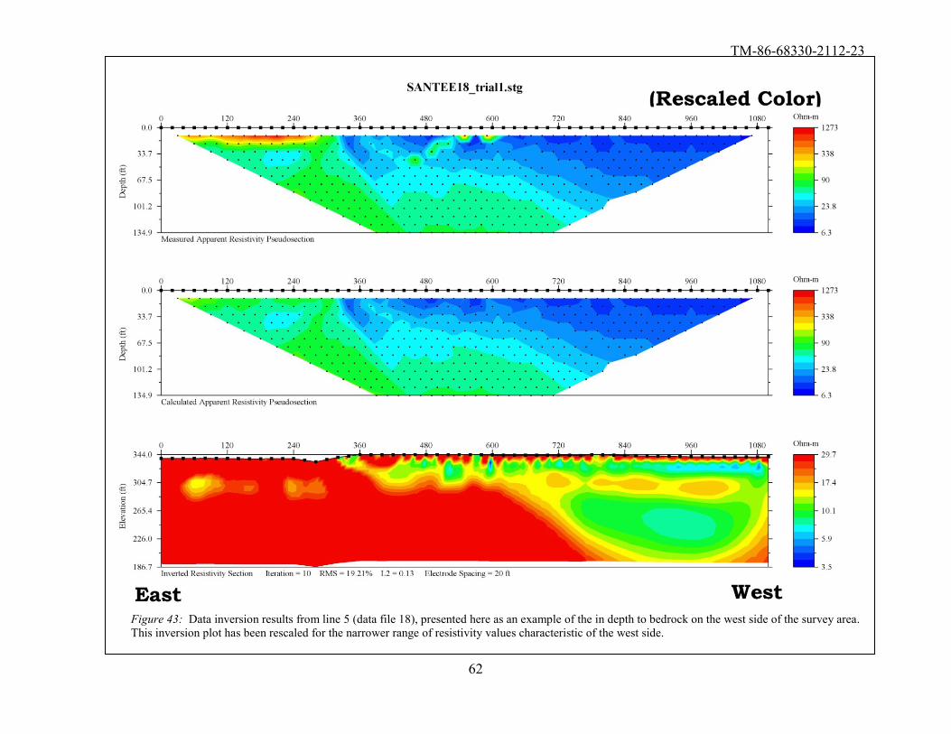
62
Figure 43: Data inversion results from line 5 (data file 18), presented here as an example of the in depth to bedrock on the west side of the survey area.
This inversion plot has been rescaled for the narrower range of resistivity values characteristic of the west side.
TM-86-68330-2112-23
63
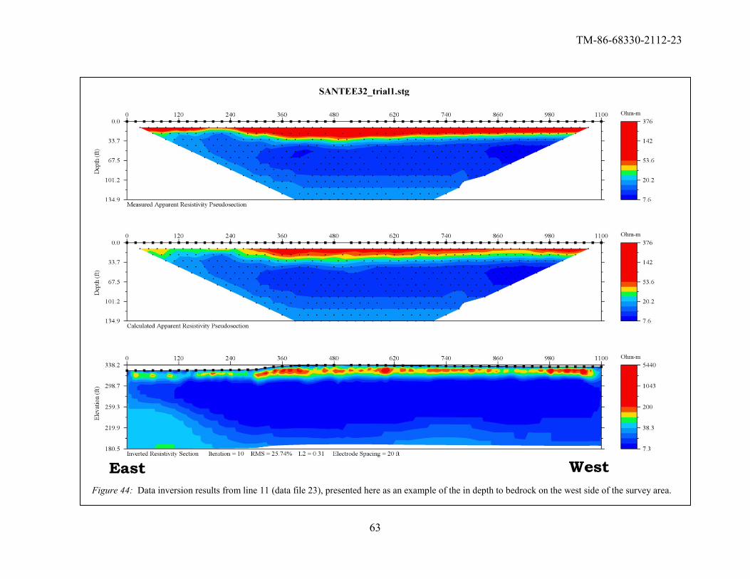
Figure 44: Data inversion results from line 11 (data file 23), presented here as an example of the in depth to bedrock on the west side of the survey area.
TM-86-68330-2112-23
64
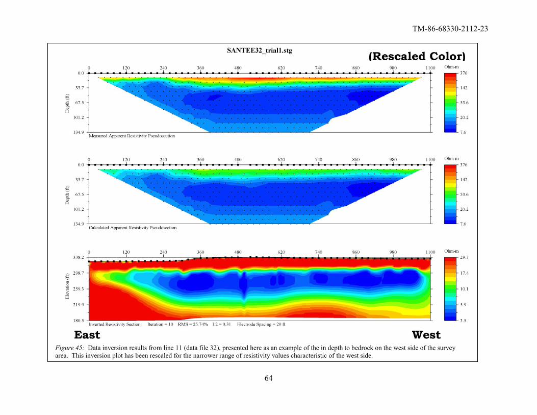
Figure 45: Data inversion results from line 11 (data file 32), presented here as an example of the in depth to bedrock on the west side of the survey
area. This inversion plot has been rescaled for the narrower range of resistivity values characteristic of the west side.
TM-86-68330-2112-23
65
4.4 Three-Dimensional Visualization
To better visualize the top of bedrock across the entire project site, three
dimensional data gridding and visualization software was utilized to interpolate an
interpreted elevation of the top-of-bedrock surface across multiple data files. This
task was achieved through the following steps:
1) Plot each 2D resistivity profile in absolute elevation versus line-distance.
2) Interpret and manually pick/digitize the top of bedrock (TOB) along each
2D resistivity cross-section based on the resistivity distribution along each
line to obtain elevation and line-distance coordinates for each pick of
TOB. (Interpretation is qualitative and based on resistivity distributions
and gradients along each profile and is not based on a single contour or
value of resistivity assumed for bedrock across the entire site).
3) Convert the line-distance values for each TOB pick to Northing and
Easting coordinates based on GPS survey data for each resistivity profile.
4) Interpolate TOB picks across the entire survey area using a three-
dimensional Kriging interpolation method to obtain a 3D surface
representing the interpreted top of bedrock.
5) Generate 3D images where the 2D resistivity profiles are plotted along
with the final 3D interpolated TOB surface.
Any interpolation process can introduce artifacts into the interpolated data when
there are drastically different input data values close to each other in space, where
the interpolant is required to honor each input datum. However, the resistivity
data presented herein are generally very good quality, and modeled resistivity
distributions and interpreted TOB picks are in very good agreement at line
intersection points. Therefore, the resultant interpretation and visualization of the
resistivity data clearly shows a relatively smooth trend in the TOB, where depth to
TOB generally increases as you go from the east side to the west side of the
survey area.
Figures 46 through 49 are presented for data visualization purposes only, and
bedrock depths should only be inferred at locations that lie close to a resistivity
profile. A vertical exaggeration factor of 2 has been used in Figures 46 through
49 for visualization purposes. In addition to the 3D visualization of the interpreted
TOB presented in Figures 46-49, Figure 50 provides a 2D shaded relief map and
contour plot of the interpreted TOB elevations in map-view. Here, the shaded
relief map has no vertical exaggeration and utilizes a grey-scale to represent TOB
elevations. Labeled elevation contours have been added at a 5-foot contour
interval. Lastly, we recommend that the interpretation and developed TOB
surface be verified by drilling near several resistivity survey lines.
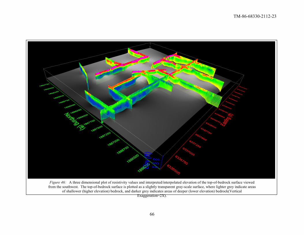
TM-86-68330-2112-23
66
Figure 46: A three dimensional plot of resistivity values and interpreted/interpolated elevation of the top-of-bedrock surface viewed
from the southwest. The top-of-bedrock surface is plotted as a slightly transparent gray-scale surface, where lighter grey indicate areas
of shallower (higher elevation) bedrock, and darker grey indicates areas of deeper (lower elevation) bedrock(Vertical
Exaggeration=2X).
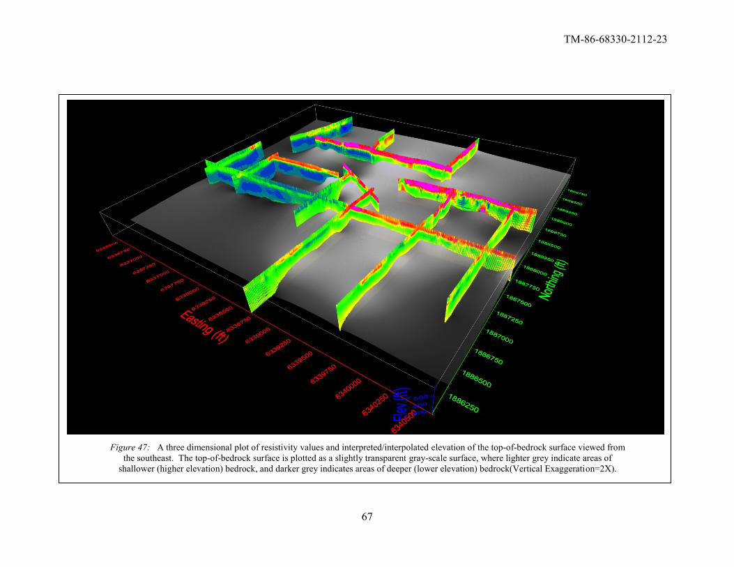
TM-86-68330-2112-23
67
Figure 47: A three dimensional plot of resistivity values and interpreted/interpolated elevation of the top-of-bedrock surface viewed from
the southeast. The top-of-bedrock surface is plotted as a slightly transparent gray-scale surface, where lighter grey indicate areas of
shallower (higher elevation) bedrock, and darker grey indicates areas of deeper (lower elevation) bedrock(Vertical Exaggeration=2X).
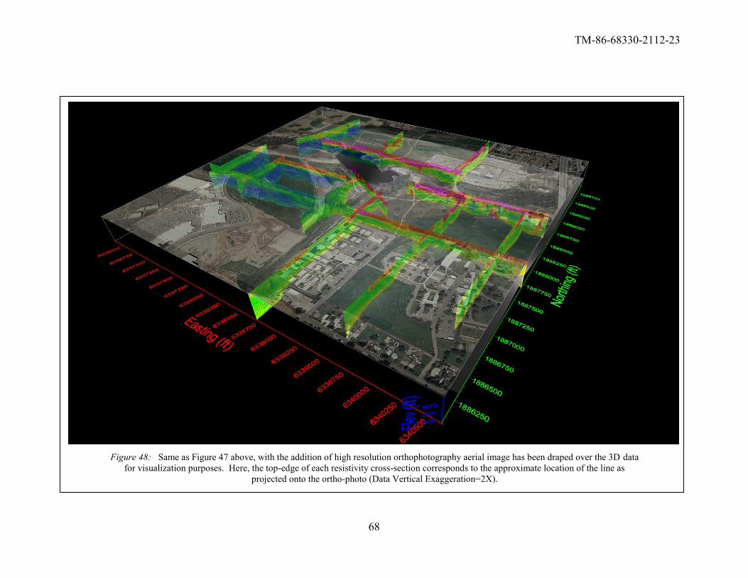
TM-86-68330-2112-23
68
Figure 48: Same as Figure 47 above, with the addition of high resolution orthophotography aerial image has been draped over the 3D data
for visualization purposes. Here, the top-edge of each resistivity cross-section corresponds to the approximate location of the line as
projected onto the ortho-photo (Data Vertical Exaggeration=2X).
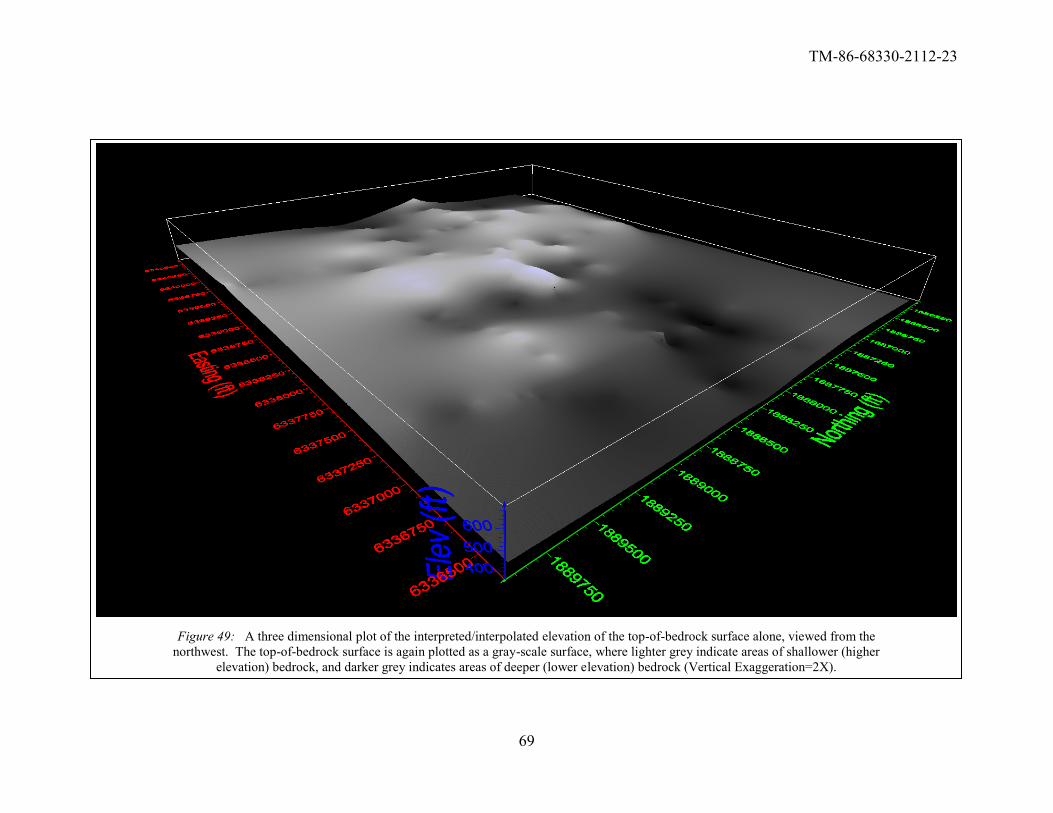
TM-86-68330-2112-23
69
Figure 49: A three dimensional plot of the interpreted/interpolated elevation of the top-of-bedrock surface alone, viewed from the
northwest. The top-of-bedrock surface is again plotted as a gray-scale surface, where lighter grey indicate areas of shallower (higher
elevation) bedrock, and darker grey indicates areas of deeper (lower elevation) bedrock (Vertical Exaggeration=2X).
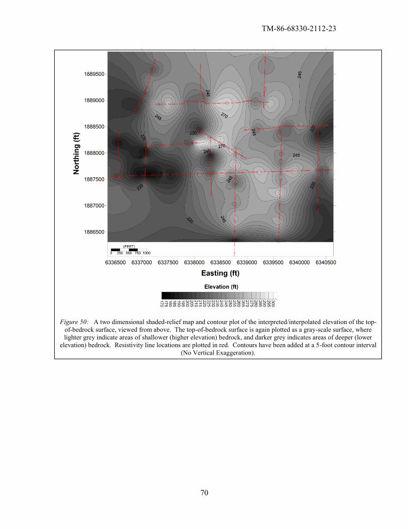
TM-86-68330-2112-23
70
Figure 50: A two dimensional shaded-relief map and contour plot of the interpreted/interpolated elevation of the top-
of-bedrock surface, viewed from above. The top-of-bedrock surface is again plotted as a gray-scale surface, where
lighter grey indicate areas of shallower (higher elevation) bedrock, and darker grey indicates areas of deeper (lower
elevation) bedrock. Resistivity line locations are plotted in red. Contours have been added at a 5-foot contour interval
(No Vertical Exaggeration).
TM-86-68330-2112-23
71
References
1. Blatchford, Douglas B.; Santee Basin Aquifer Recharge Study; US Bureau
of Reclamation Technical Memorandum; February 2011
2. Morgan, Frank Dale; Self Potential and Resistivity for the Detection and
Monitoring of Earthen Dam Seepage; Massachusetts Institute of
Technology: Department of Earth, Atmospheric and Planetary Sciences,
Earth Resources Laboratory; March 2001
3. Sjödahl, Pontus; Resistivity investigation and monitoring for detection of
internal erosion and anomalous seepage in embankment dams; Lund
University: Doctoral Thesis; March 2006
4. Aizebeokhai, Ahzegbobor Philips; 2D and 3D geoelectrical resistivity
imaging: Theory and field design; Scientific Research and Essays Vol.
5(23), pp. 3592-3605; December, 2010
5. Ganse, Andrew A.; A Geophysical Inverse Theory Primer; University of
Washington: Applied Physics Laboratory and Department of Earth and
Space Sciences; March 2008
6 Palacky, G.J.; Resistivity Characteristics of Geologic Targets in M.N.
Nabighian; ed. Electromagnetic methods in applied Geophysics, vol. 1,
SEG Investigations in Geophysics Series Number 3.1897
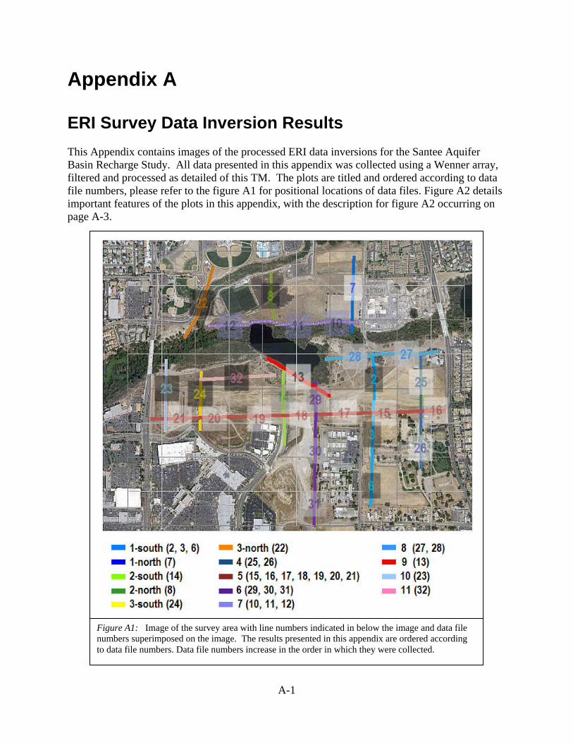
Appendix A ERI Survey Data Inversion Results This Appendix contains images of the processed ERI data inversions for the Santee Aquifer Basin Recharge Study. All data presented in this appendix was collected using a Wenner array, filtered and processed as detailed of this TM. The plots are titled and ordered according to data file numbers, please refer to the figure A1 for positional locations of data files. Figure A2 details important features of the plots in this appendix, with the description for figure A2 occurring on page A-3.
Figure A1: Image of the survey area with line numbers indicated in below the image and data file numbers superimposed on the image. The results presented in this appendix are ordered according to data file numbers. Data file numbers increase in the order in which they were collected.
A-1
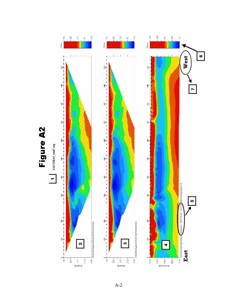
A-2

Figure A2: Explanation of graphical standard output of inversion results from Earth Imager™.
1. Inversion titles for this project will always appear in this format: SANTEE(data file number)_trial(number of times data set has been altered and saved).stg
2. Collected data set displayed as a pseudosection. Black dots are locations of individual data points. A color contour plot has been formatted for
the data set to display apparent resistivity values. The note at the lower left of this plot indicates it is a “Measured Apparent Resistivity Pseudosection.” This note corresponds with a collected data. This plot is displayed with distance along the data file (in feet) for the horizontal axis and depth (in feet) along the vertical axis.
3. Synthetic calculated data set displayed as a pseudosection. This plot presents the synthetic data set that is calculated from the final resulting inversion. Black dots are locations of individual calculated data points. A color contour plot has been formatted for the data set to display apparent resistivity values. The note at the lower left of this plot indicates it is a “Calculated Apparent Resistivity Pseudosection.” This note corresponds with a synthetic calculated data set. This plot is displayed with distance along the data file (in feet) for the horizontal axis and depth (in feet) along the vertical axis.
4. This plot is the final result of the inversion process. It is a model of subsurface electrical resistivity, and is the output from the inversion process that is used for interpreting subsurface geologic structure. The note at the lower left of this plot indicates it is an “Inverted Resistivity Section.” This note corresponds with a model of subsurface resistivity resulting from the inversion process. This plot is displayed with distance along the data file (in feet) for the horizontal axis and elevation (in feet) along the vertical axis.
5. Inverted resistivity sections appear with calculation statistics listed below the plot. The iteration number refers to how many times the subsurface was altered, a synthetic data set was calculated and the collected and calculated data sets were compared. The first iteration for all inversions done for this project used a homogenous subsurface model with the resistivity equal to that of the average resistivity value of the data file. The RMS stands for root mean square (in mathematics it is also known as the quadratic mean). The root mean square is a statistical measure of a varying quantity. The RMS is calculated between the calculated data and the collected data and listed here. The lower the RMS percentage, the greater equivalence there is between the collected and calculated data sets. The L2 number listed here is another measure of data misfit based on the normalization of a least squares regression of the calculated data. When the L2 value is equal to, or less than 1.0, the inversion has converged, meaning that the collected and calculated data sets are reasonable equivalent.
6. Each plot has its own color scale of resistivity values. Plots that occur in the same inversion figure will often have equal color scales for the measured and calculated apparent resistivity pseudosections and a differing color scale for the inverted resistivity section. The color scales for this project are all logarithmic, which yields greater color variation for more conductive values (cooler colors) and less color variation for highly resistive values (warmer colors). All resistivity and apparent resistivity color scales are presented in ohm-meters, the SI unit for electrical resistivity.
7. Inversion of collected data files for this project have been annotated with cardinal directions, so that the orientation of the data file may be determined with respect to the survey area.
A-3
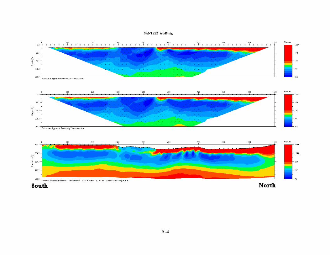
A-4
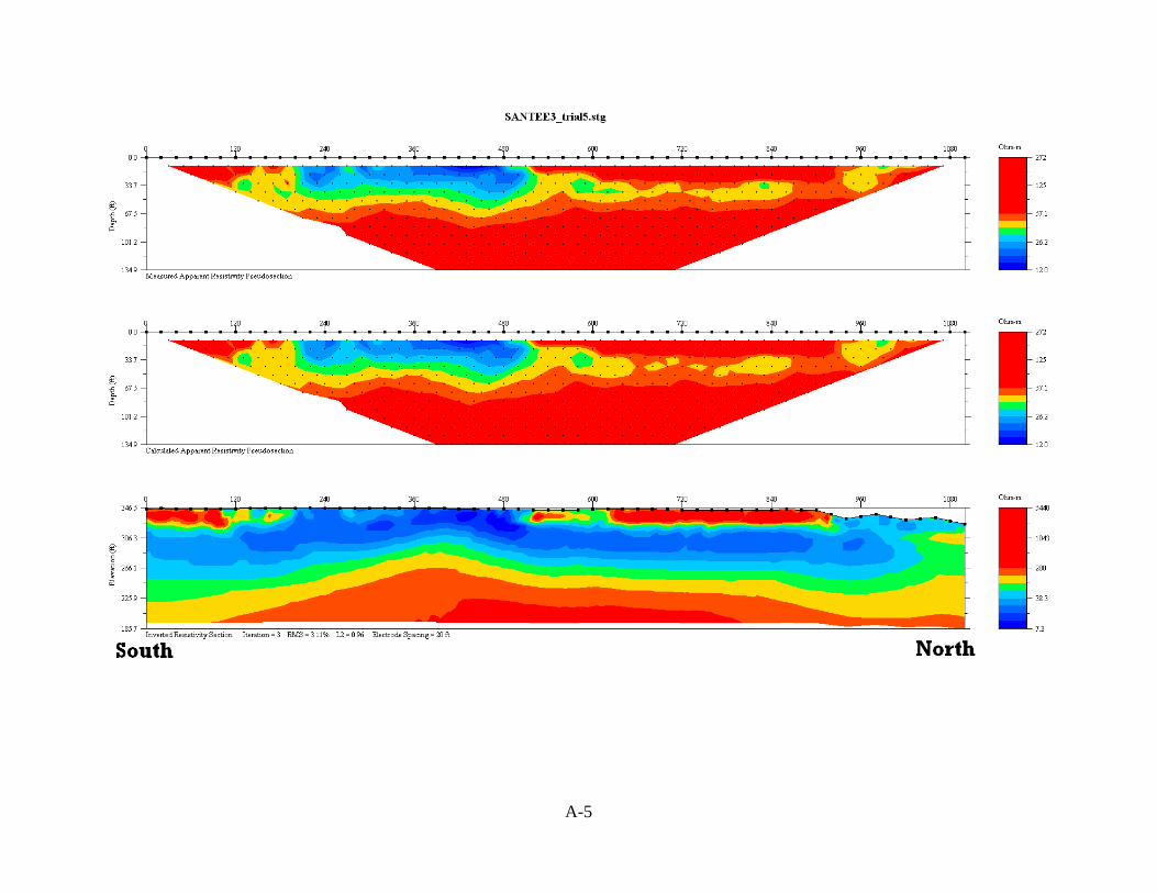
A-5
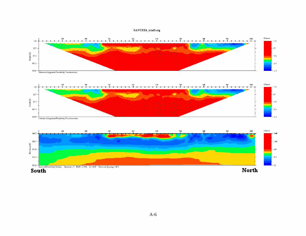
A-6
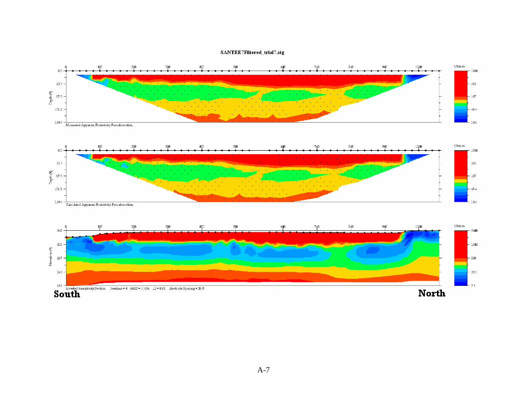
A-7
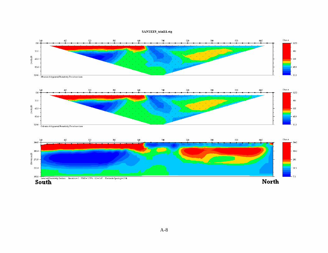
A-8
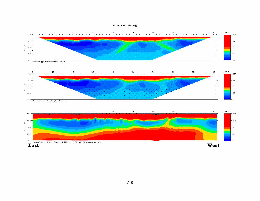
A-9
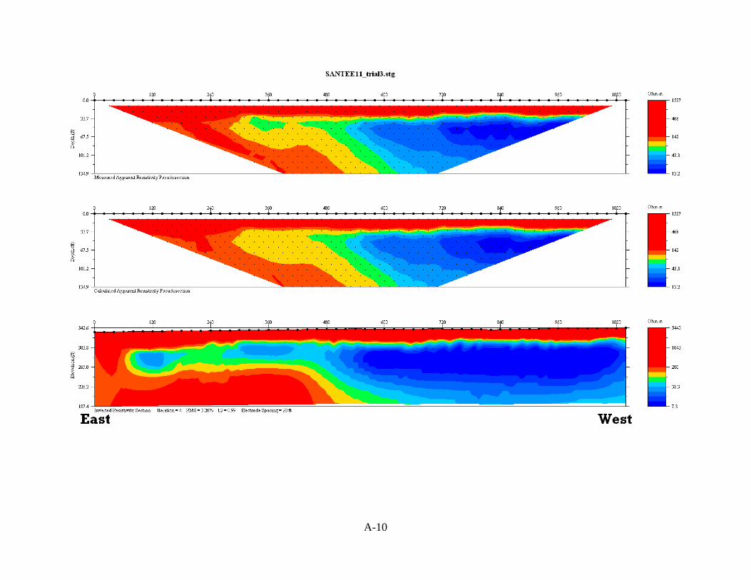
A-10
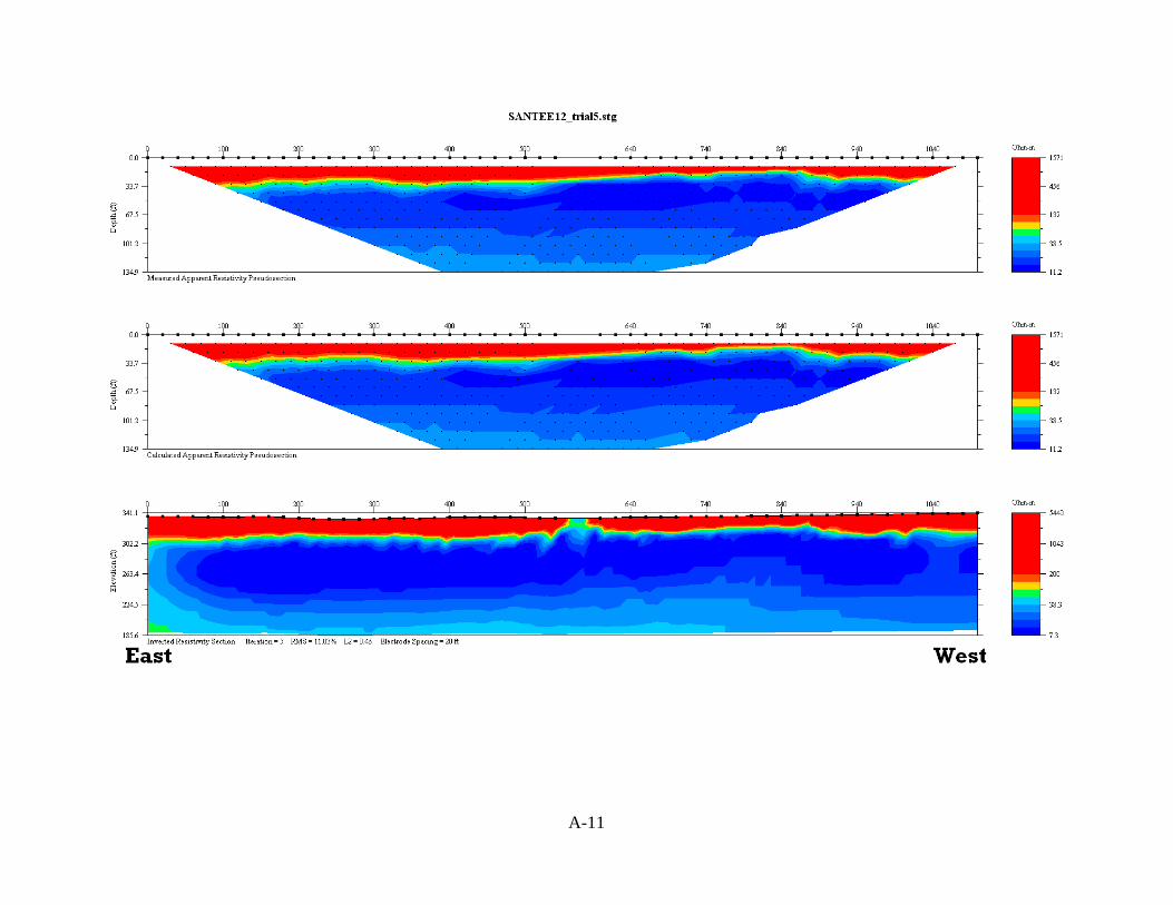
A-11
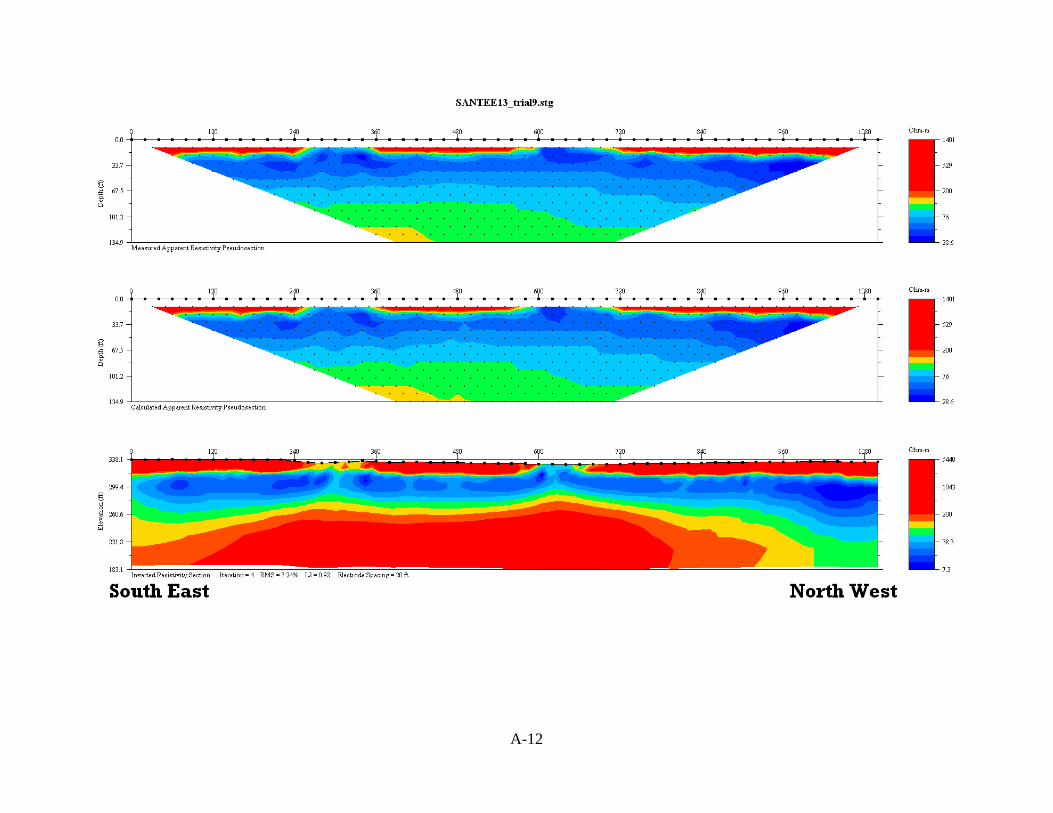
A-12
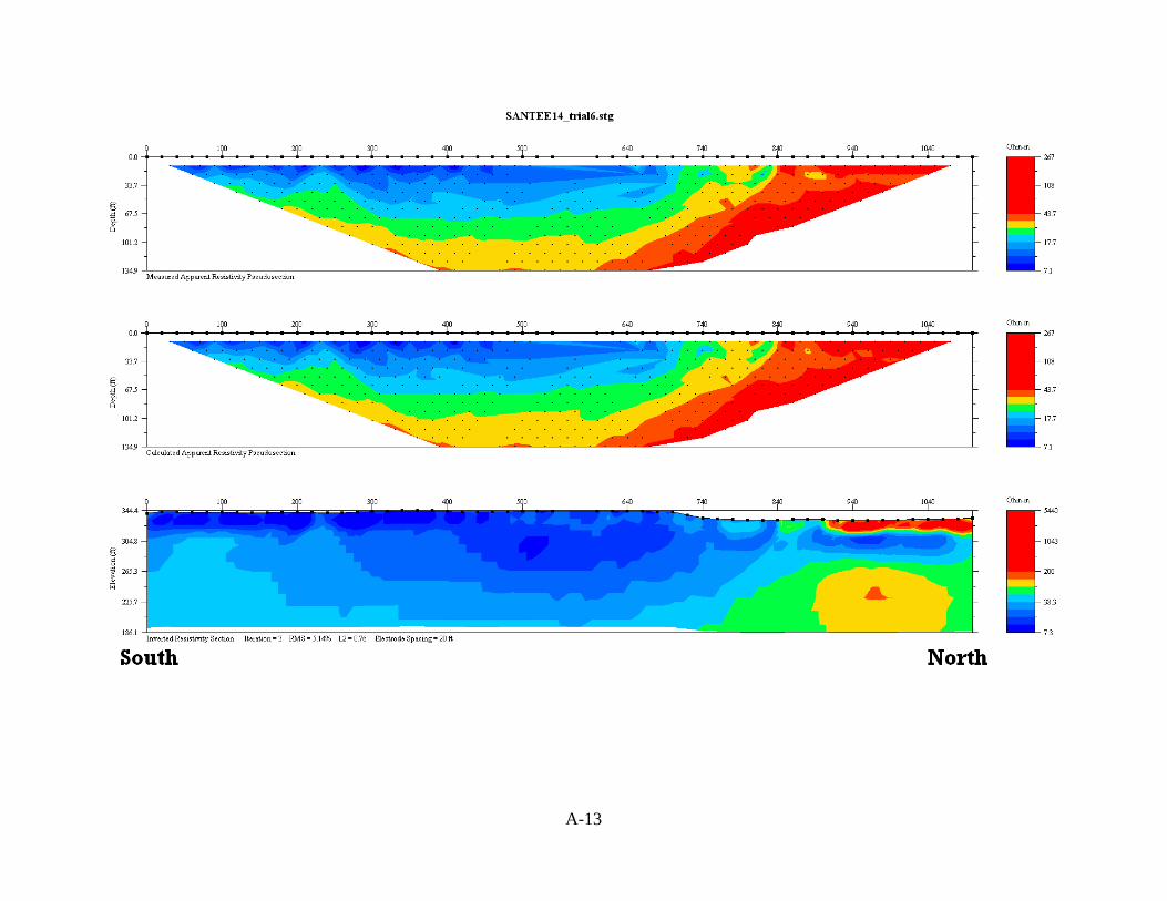
A-13
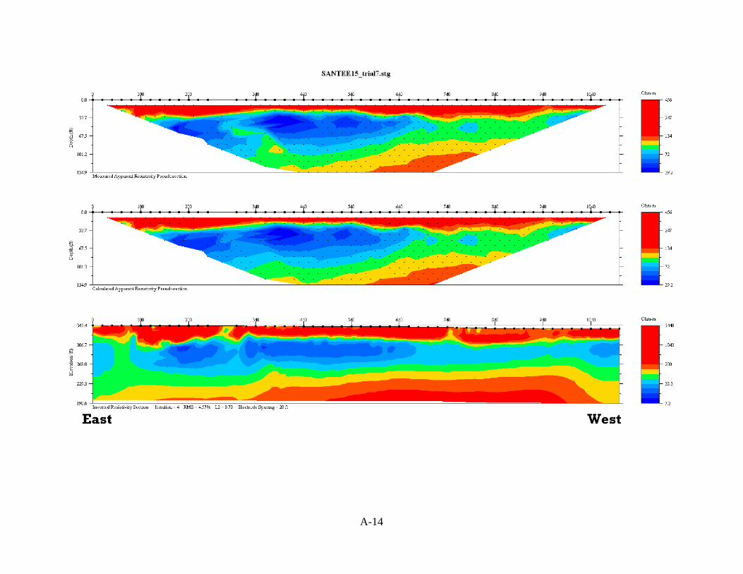
A-14
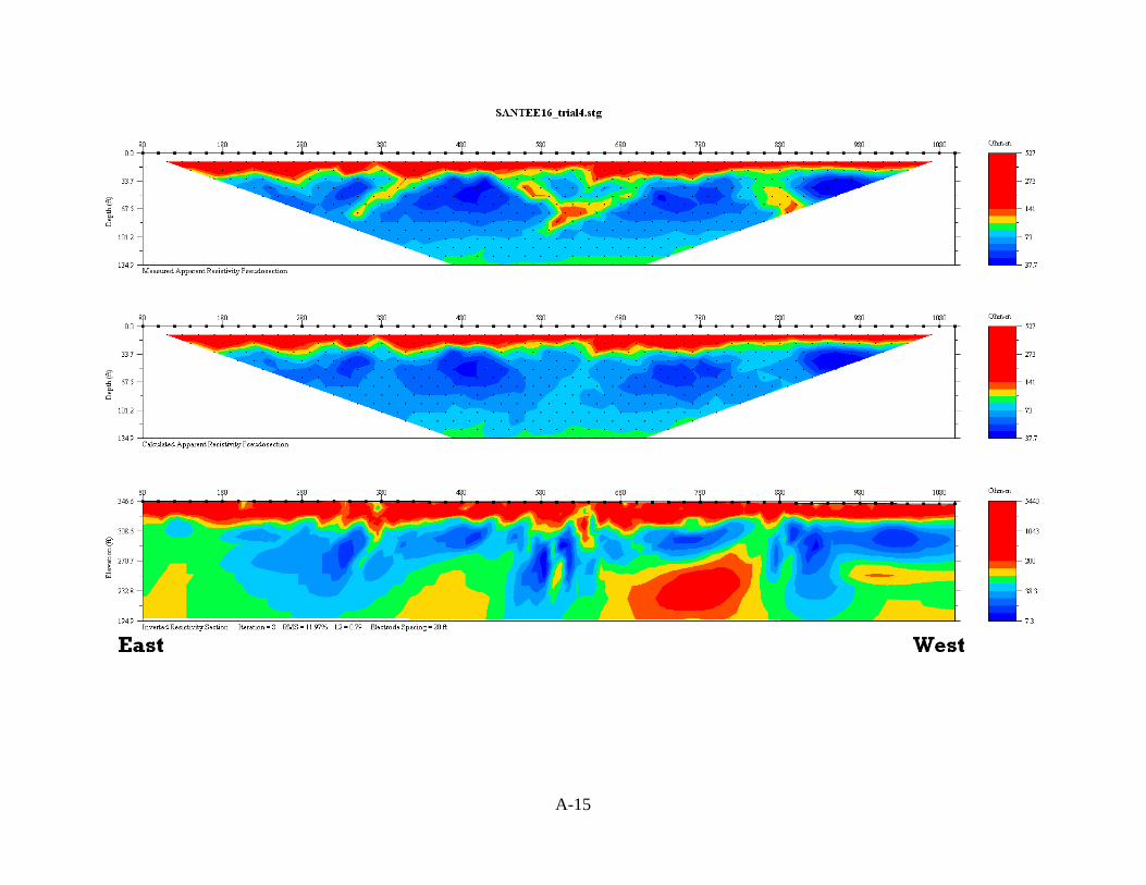
A-15
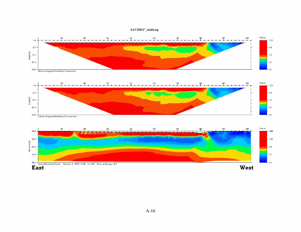
A-16
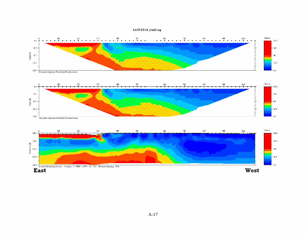
A-17
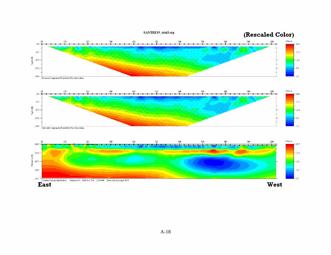
A-18
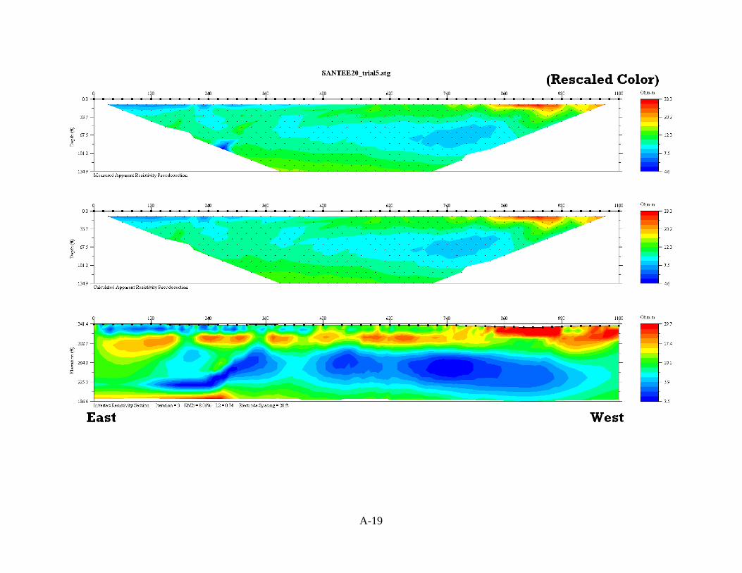
A-19
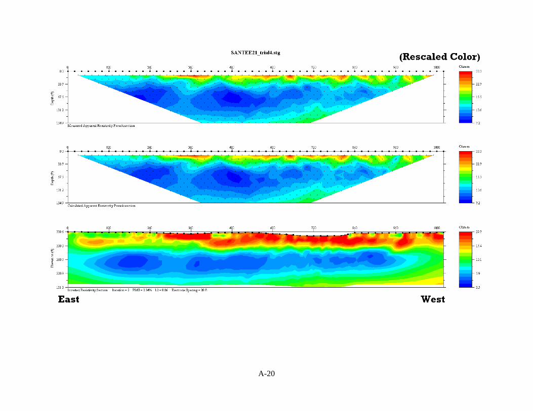
A-20
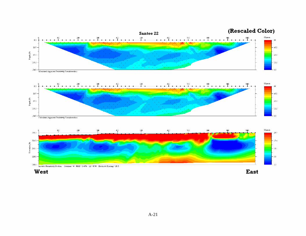
A-21
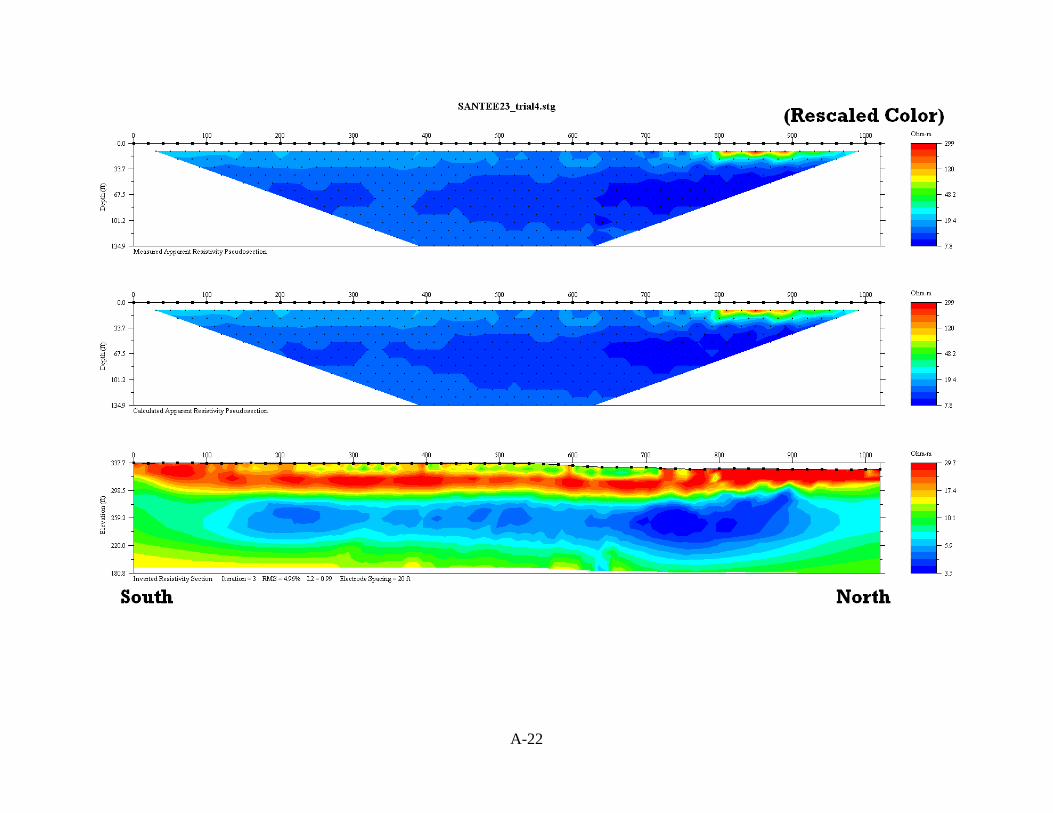
A-22
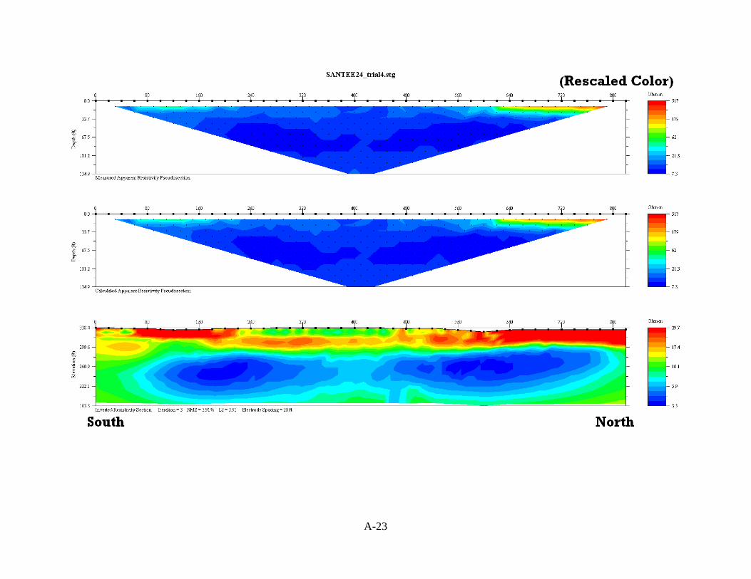
A-23
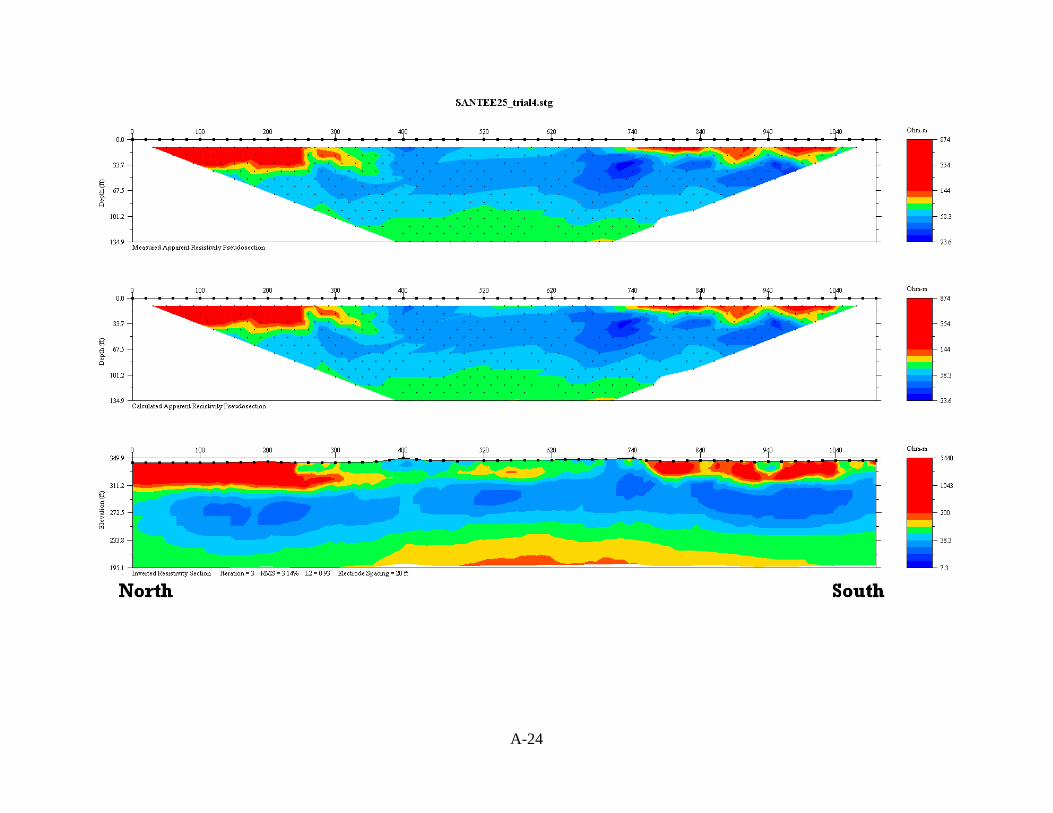
A-24
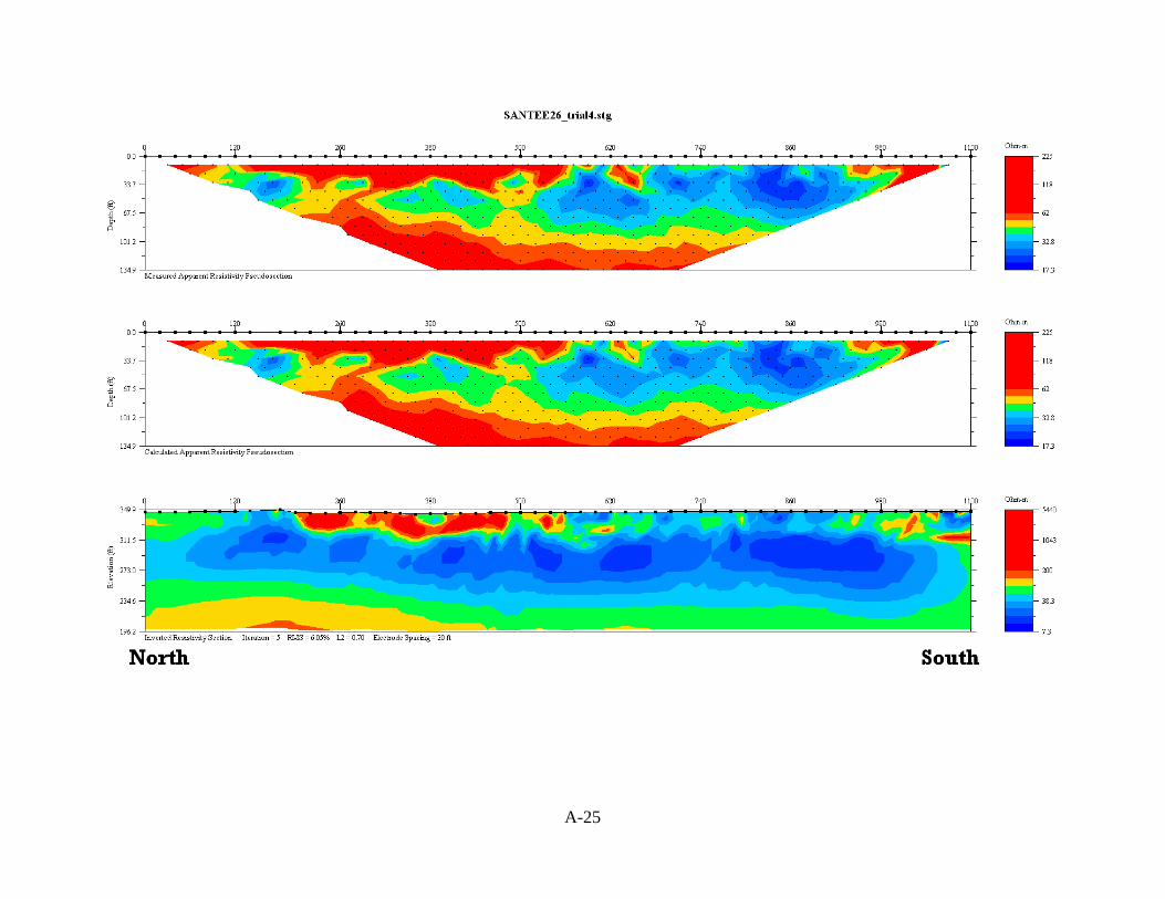
A-25
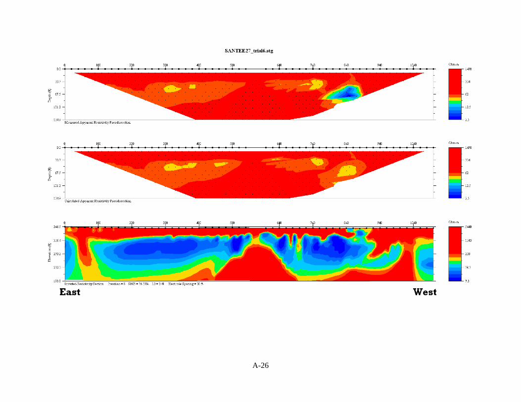
A-26
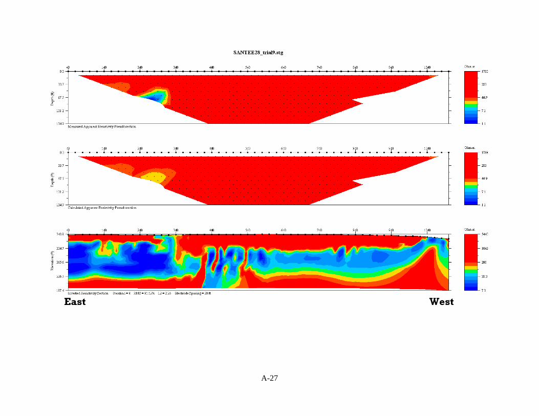
A-27
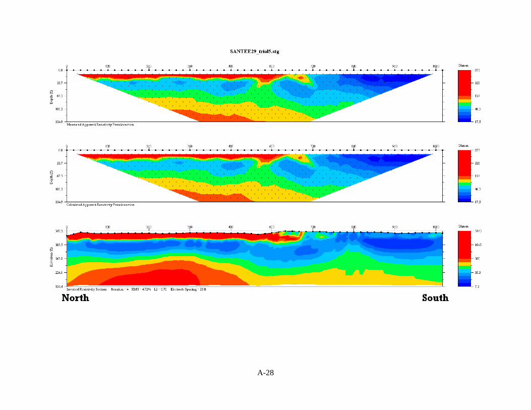
A-28
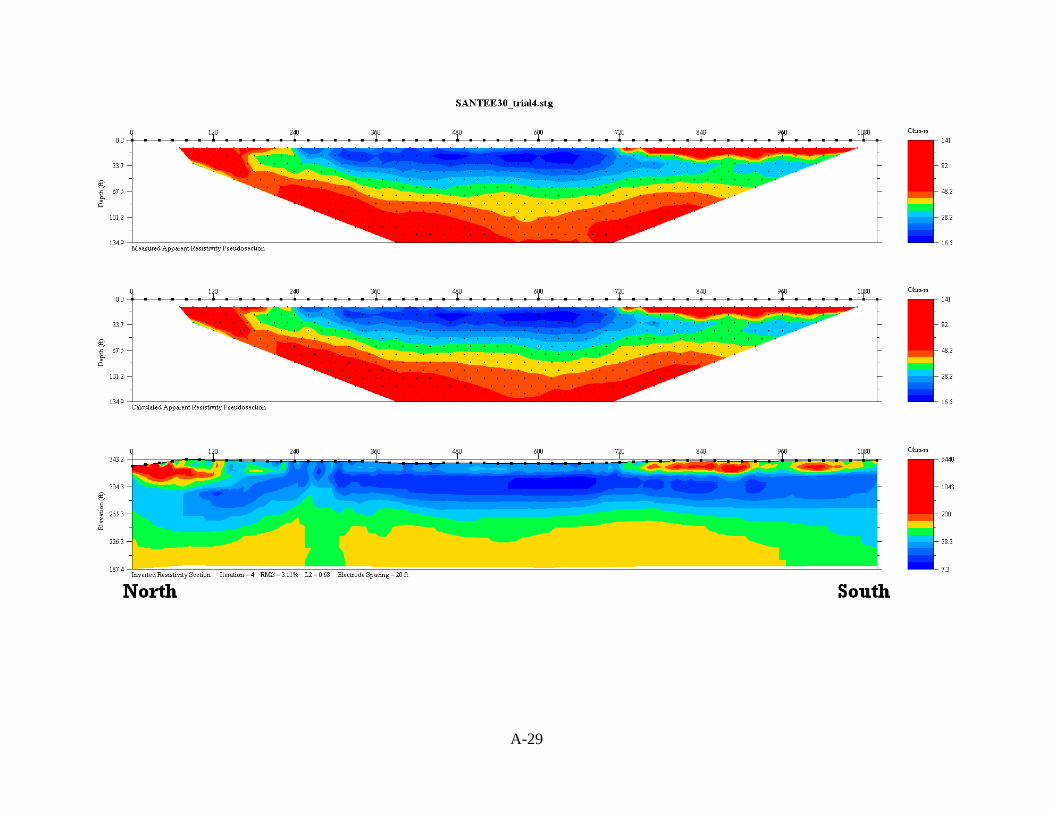
A-29
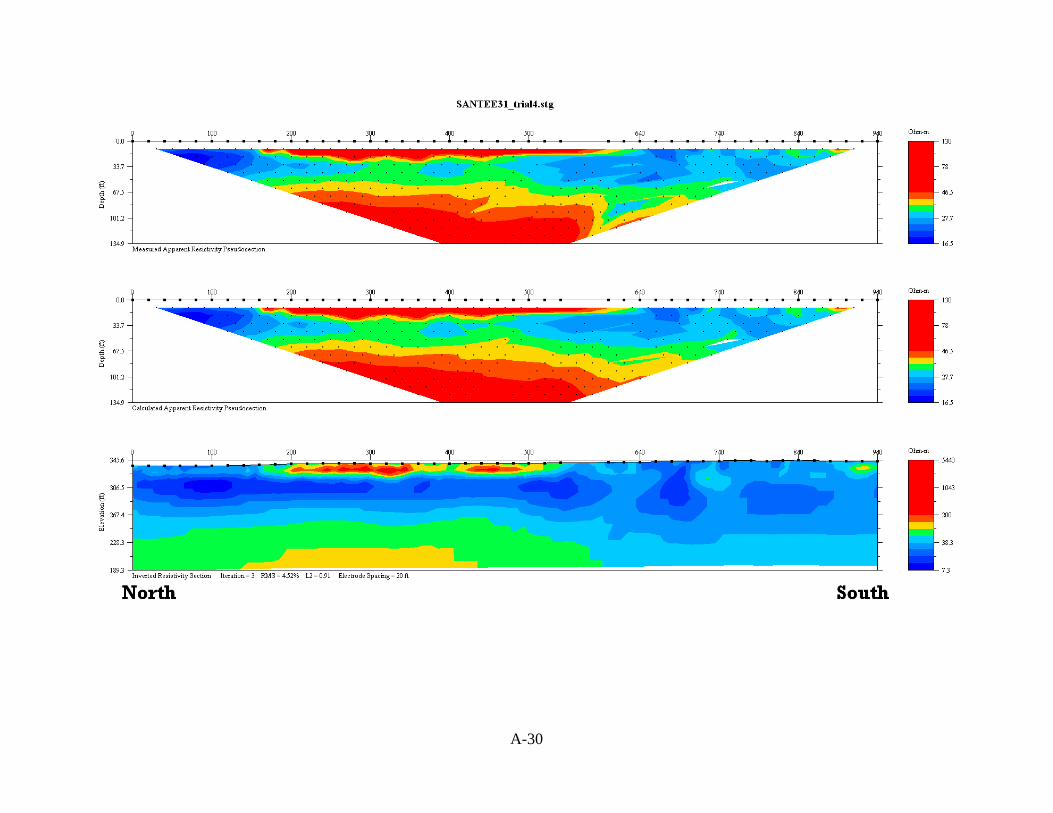
A-30
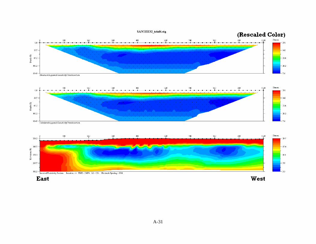
A-31
B-1
Appendix B
Glossary of Selected Geophysical Terms
Apparent resistivity – The resistivity of homogenous, isotropic ground which would give the same
voltage-current relationship as measured.
Array – In resistivity, an array is the arrangement of electrodes, also called configuration.
Competent (geologic) – A bed which retains its stratigraphic thickness under stress. It folds or breaks
under stress, in comparison with adjacent incompetent beds which tend to flow.
Conductive material (electrical) – Any material which allows the passage of electric current through its
volume.
Electric Current – Is a flow of electric charge through a medium. Types of electric circuits encountered
in geophysics include conduction currents (flow of electrons), electrolytic conduction (flow of ions), and
di-electric conduction (currents involved in capacitive storage of electric charge).
Electric Potential – The electric potential (a scalar quantity denoted by φ, φE or V and also called the
electric field potential or the electrostatic potential) at a point is equal to the electric potential energy
(measured in joules) of a charged particle at that location divided by the charge (measured in coulombs)
of the particle. Electric potentials involved in geophysics include the zeta potential, liquid junction and
shale potentials, electrolytic contact potential, electrokinetic potential, and polarization potentials.
Electrical Resistance – The opposition to the passage of an electric current through that element.
Electrical Resistivity – The electrical resistance per unit length of a unit cross-sectional area of a
material. The unit of electrical resistivity is the ohm⋅metre (Ω⋅m).
Electrodes – A piece of metallic material that is used as an electric contact with a nonmetal. Can refer
to a grounding contact, to metallic minerals in a rock, or to electric contacts in laboratory equipment.
Four-pin resistivity survey – Also known as the Wenner Method, involves placing 4 probes in the earth
at equal spacing. The probes are connected with wires to the ground resistance test set. The test set
passes a known amount of current through the outer two probes and measures the voltage drop
between the inner two probes. Using ohms law it will output a resistance value, which can then be
converted to a resistivity value.
Forward Model – The technique of determining what a given survey would measure in a given
formation and environment by applying a set of theoretical equations for the survey response.
B-2
Geometric factor (K) – A numerical factor used to multiply the voltage-to-current ratio from
measurements between electrodes to give apparent resistivity. Geometric factor is dependent on the
type of electrode array and spacing used.
Geophysical – Study of the Earth by quantitative physical methods.
Half-space – A mathematical model bounded only by one plane surface, i.e., the model is so large in
other dimensions that only the one boundary affects the results. Properties within the model are usually
assumed to be homogenous and isotropic, though other models are also used.
Heterogeneous – Lack of spatial uniformity.
Homogeneous – The same throughout; uniformity of a physical property throughout the material.
Inversion – Deriving from field data a model to describe the subsurface that is consistent with the data.
Determining the cause from observation of effects.
Masked – The effect whereby a highly conductive layer near the surface dominates resistivity
measurements so as to make undetectable the effects of deeper resistivity variations.
Noisy – Noise in electrical surveying can be due to interference from power lines, motor-generator or
electric components, atmospheric electrical discharges (sferics), or low-frequency magnetotelluric
phenomena. Even near surface elements such as vegetation, saturated sediments, underground utility
pipes, etc. can create noise in electrical surveys.
Ohm’s Law – The current (I) through a conductor between two points is directly proportional to the
potential difference (V) across the two points, introducing the constant of proportionality, resistance (R).
Ohm-meter – A unit of resistivity, measuring the extent to which a substance offers resistance to
passage of an electric current. The resistivity of a conductor in ohm meters is defined to be its resistance
(in ohms) multiplied by its cross-sectional area (in square meters) divided by its length (in meters).
Physical material property – Any property that is measurable whose value describes a physical system's
state. It is an intensive, often quantitative property of a material, usually with a unit that may be used
as a metric of value to compare the benefits of one material versus another to aid in materials selection.
The value of a physical property depends upon material type (rock, soil, etc), alteration or weathering,
how different components are mixed, texture, grain size, porosity, connectivity of fluid pathways, types
of interstitial fluids etc. Thus the physical property value is situation dependent. Ideally, geophysical
surveys using samples or borehole techniques can be carried out to determine the relationship between
the different components of the earth and the physical property value. It is often possible to use
information in the literature or from previous case histories to estimate a likely range for a physical
B-3
property associated with a particular rock or soil unit. The main quantity to be ascertained is whether
there is a significant contrast of the property for the target and host. For instance, if you are looking for
a buried pipe, you know that its conductivity is substantially greater than the host ground and hence
electrical conductivity will be a diagnostic physical property.
Psuedosection – A plot of electrical measurements or calculations as a function of position and
electrode separation. A psuedosection indicates how the parameter varies with location and depth, but
it can only be converted with a two-dimensional model by inversion.
Resistive material (electrical) – Any material which opposes the passage of electric current through its
volume.
Resistivity value – The property of a material which resists the flow of electrical current. Also called
specific resistance. The ratio of electric-field intensity to current density.
Stacked –Stacked data is used to attenuate noise by effectively averaging multiple measurements in the
stacking operation.
Vadose zone – A subsurface zone containing water under pressure less than that of the atmosphere,
including water held by capillarity; and containing air or gases generally under atmospheric pressure.
This zone is limited above by the land surface and below by the surface of the zone of saturation, i.e. the
water table.