Geophysical Investigation of the T and T Mine Complex, Preston County,West Virginia

Jennifer S. Mabie

Thesis submitted to the College of Arts andSciences at West Virginia University

in partial fulfillment of the requirementsfor the degree of

Master of Sciencein

Geology

Committee Members:

Dr. Thomas H. Wilson, chair

Dr. Timothy Warner

Mr. Richard Hammack, USDOE

Department of Geology and Geography

Morgantown, WV

2003

Keywords: Geophysics, Airborne Geophysics, Remote Sensing, Terrain Conductivity,

Resistivity, Soundings, Preston County

ABSTRACT

Geophysical Investigations of the T and T Mine Complex, Preston County, WestVirginia

Jennifer S. Mabie

The U.S. Department of Energy National Energy and Technology Laboratory have utilizedan airborne platform with remote sensing technologies consisting of a multi-spectral scannerand airborne electromagnetic conductivity technologies to provide a rapid reconnaissance ofwatershed areas. Airborne surveys were flown over the T&T Mine Complex, located inPreston County, West Virginia. The electromagnetic and thermal anomalies observed in theairborne data were compared to mine maps to correlate anomalous features with mine poolsand ground water discharge points that may represent acid mine drainage (AMD). Surfacegeophysical studies were performed to delineate the conductivity anomalies observed in theairborne data. The geophysical surveys were not able to resolve the mine pool at a depth of90 meters; however, there was resolution between airborne and ground survey results up to adepth of 40 meters. The thermal data was not able to resolve groundwater discharge pointsthat may represent AMD.

iii

Acknowledgements

I would like to thank many of the individuals and organizations that helped to make

this work possible. I would like the thank Terry Ackman and Richard Hammack from the

USDOE/NETL, Clean Water Team for the providing me with an opportunity to participate in

the University-Partnership Program, allowing me to use the data, facilities, and equipment

belonging to the DOE. Thanks, Rick, for keeping me on task. I would also like to thank

Garret “The Fabric” Veloski and Jim Sams and other members of the Clean Water Team for

all of your help. I would like to thank Tim Warner for his time and interest in the thermal

aspects of this research project. I would like to give a special thanks to my advisor, Tom

Wilson, for the continuous support, encouragement, and patience throughout the duration of

this project and for giving me the University Partnership opportunity. Finally, I would like

to thank my family and friends who have helped me physically, emotionally, spiritually, and

financially over the years.

iv

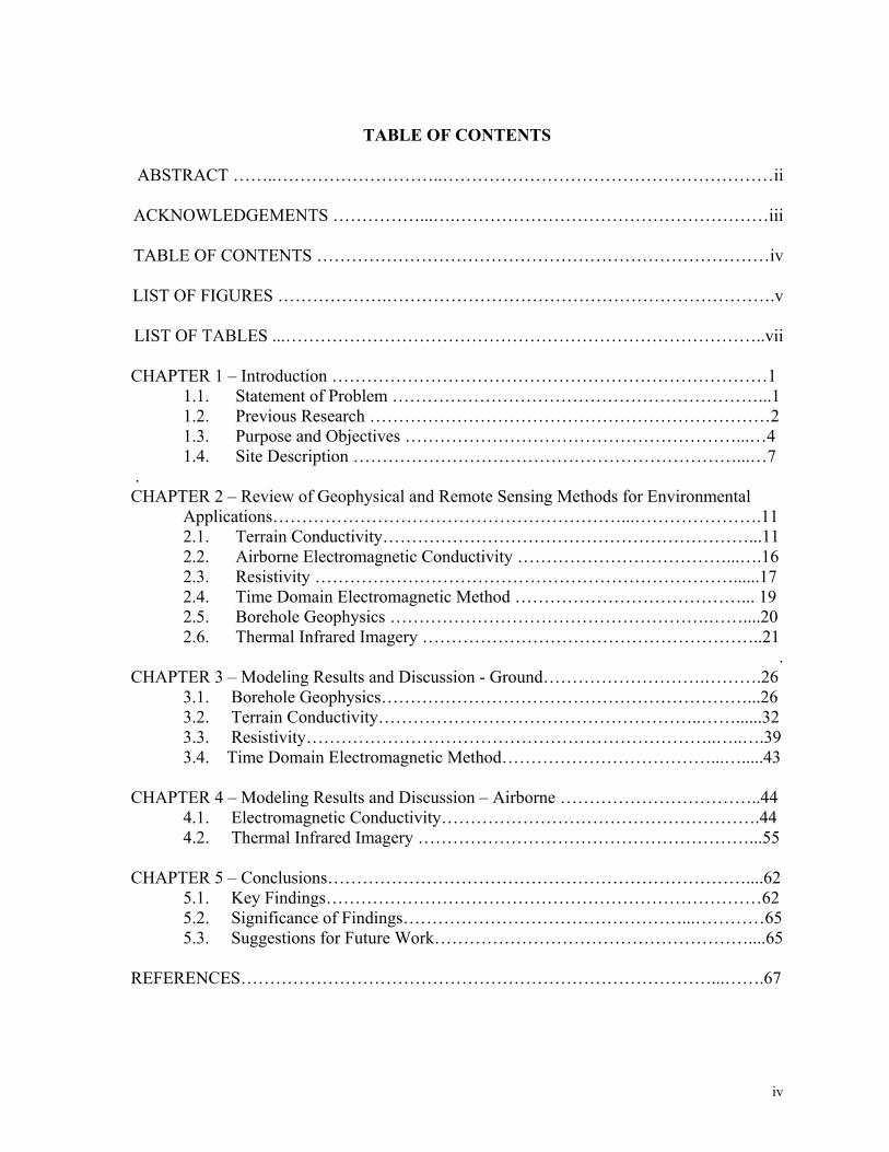
TABLE OF CONTENTS

ABSTRACT ……..………………………..…………………………………………………ii

ACKNOWLEDGEMENTS ……………...….………………………………………………iii

TABLE OF CONTENTS ……………………………………………………………………iv

LIST OF FIGURES ……………….………………………………………………………….v

LIST OF TABLES ...………………………………………………………………………..vii

CHAPTER 1 – Introduction …………………………………………………………………11.1. Statement of Problem ………………………………………………………...11.2. Previous Research ……………………………………………………………21.3. Purpose and Objectives …………………………………………………...…41.4. Site Description …………………………………………………………...…7

.CHAPTER 2 – Review of Geophysical and Remote Sensing Methods for Environmental

Applications……………………………………………………...………………….112.1. Terrain Conductivity………………………………………………………...112.2. Airborne Electromagnetic Conductivity ………………………………...….162.3. Resistivity ………………………………………………………………......172.4. Time Domain Electromagnetic Method …………………………………... 192.5. Borehole Geophysics ……………………………………………….……....202.6. Thermal Infrared Imagery …………………………………………………..21

.CHAPTER 3 – Modeling Results and Discussion - Ground……………………….……….26

3.1. Borehole Geophysics………………………………………………………...263.2. Terrain Conductivity………………………………………………..……......323.3. Resistivity……………………………………………………………..…..….393.4. Time Domain Electromagnetic Method………………………………...….....43

CHAPTER 4 – Modeling Results and Discussion – Airborne ……………………………..444.1. Electromagnetic Conductivity……………………………………………….444.2. Thermal Infrared Imagery …………………………………………………...55

CHAPTER 5 – Conclusions………………………………………………………………....625.1. Key Findings…………………………………………………………………625.2. Significance of Findings…………………………………………...…………655.3. Suggestions for Future Work………………………………………………....65

REFERENCES………………………………………………………………………...…….67

v

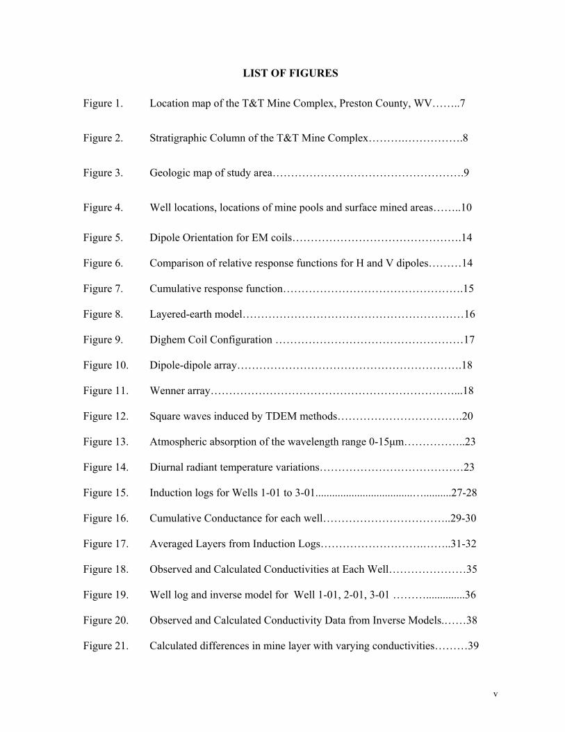
LIST OF FIGURES

Figure 1. Location map of the T&T Mine Complex, Preston County, WV……..7

Figure 2. Stratigraphic Column of the T&T Mine Complex……….…………….8

Figure 3. Geologic map of study area…………………………………………….9

Figure 4. Well locations, locations of mine pools and surface mined areas……..10

Figure 5. Dipole Orientation for EM coils……………………………………….14

Figure 6. Comparison of relative response functions for H and V dipoles………14

Figure 7. Cumulative response function………………………………………….15

Figure 8. Layered-earth model……………………………………………………16

Figure 9. Dighem Coil Configuration ……………………………………………17

Figure 10. Dipole-dipole array…………………………………………………….18

Figure 11. Wenner array…………………………………………………………...18

Figure 12. Square waves induced by TDEM methods…………………………….20

Figure 13. Atmospheric absorption of the wavelength range 0-15µm……………..23

Figure 14. Diurnal radiant temperature variations…………………………………23

Figure 15. Induction logs for Wells 1-01 to 3-01...................................…..........27-28

Figure 16. Cumulative Conductance for each well……………………………..29-30

Figure 17. Averaged Layers from Induction Logs……………………….……..31-32

Figure 18. Observed and Calculated Conductivities at Each Well…………………35

Figure 19. Well log and inverse model for Well 1-01, 2-01, 3-01 ………..............36

Figure 20. Observed and Calculated Conductivity Data from Inverse Models.……38

Figure 21. Calculated differences in mine layer with varying conductivities………39

vi

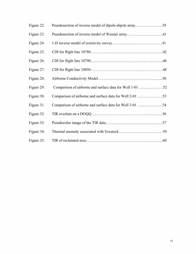
Figure 22. Psuedosection of inverse model of dipole-dipole array…………………39

Figure 23. Psuedosection of inverse model of Wenner array……………………….41

Figure 24. 1-D inverse model of resistivity survey…………………………………41

Figure 25. CDI for flight line 10780………………………………………...……....42

Figure 26. CDI for flight line 10790…………………………………….…..….…...46

Figure 27. CDI for flight line 10850…………………………………...….….….….48

Figure 28. Airborne Conductivity Model………………………………….…..…....50

Figure 29. Comparison of airborne and surface data for Well 1-01 …….…………52

Figure 30. Comparison of airborne and surface data for Well 2-01 ……….……….53

Figure 31. Comparison of airborne and surface data for Well 3-01 ………………..54

Figure 32. TIR overlain on a DOQQ…………………………………………….….56

Figure 33. Pseudocolor image of the TIR data……………………………….……..57

Figure 34. Thermal anomaly associated with livestock………………………..……59

Figure 35. TIR of reclaimed area…………………………………………….……...60

vii

LIST OF TABLES

Table 1. Skin depths for various airborne frequencies………………………….13

Table 2. GIS layer information………………………………………………….57

1

CHAPTER 1 – Introduction

1.1. Statement of Problem

The production of acid mine drainage (AMD) from coal mining sites in the

Appalachian area of the United States is a major environmental issue that receives much

attention in affected communities. Remedial procedures are often initiated in response to the

need to be in compliance with Surface Mining Control and Reclamation Act water quality

standards. However, reclamation efforts are usually based on very little subsurface

information. In most cases, geophysical assessment of the area is not available. Lack of

site-specific subsurface information often limits the effectiveness and increases the cost of

remedial action.

Acid mine drainage is generally associated with an increase in concentration of heavy

metals and other ionic species that increase specific conductance of ground and surface

waters. This increase in conductance makes mapping of AMD ground water contamination

using geophysical methods a low cost alternative to collecting subsurface data. Acid mine

drainage has had a significant impact on water quality in the Appalachian region for decades

and will continue to adversely affect these areas unless effective and comprehensive

remedial actions can be designed and applied.

The U. S. Department of Energy National Energy Technology Lab's (NETL) Clean

Water Team utilizes an airborne platform with four different technologies consisting of a

multi-spectral scanner (MSS) equipped with dual infrared sensors, and three geophysical

technologies: terrain conductivity, very low frequency, and magnetometry (Ackman et al.,

2000). The airborne approach identifies potential problem areas over whole watershed areas

2

in a short period of time and helps identify possible relationships between polluted areas that

might otherwise be missed by limited surface investigations.

1.2. Previous Research

Traditionally, airborne geophysical surveys have been used for the detection of

conductive ore bodies and geologic mapping. However, in recent years, studies have

demonstrated the effectiveness of airborne geophysics and remote sensing for environmental

purposes.

King and Hynes (1994) used geophysical methods to monitor acid mine drainage at

the Sudbury Igneous Complex. High quality airborne geophysical data was acquired with a

multi-coil, multi-frequency helicopter electromagnetic system over tailings areas, which are

thought to be source areas of AMD seeps. The airborne data results indicated that

anomalous areas coincided with the tailings. The airborne surveys were verified by ground-

based geophysical surveys performed with Geonics EM-31 and EM-34 terrain conductivity

instruments. Additionally, borehole electromagnetic surveys were conducted to locate the

source of the anomalous conductivity within the tailings piles. The electromagnetic

conductivity data was correlated with previously acquired resistivity data. The study showed

that the combination of airborne and ground-based geophysical investigations characterize

the three-dimensional distribution of acid-producing materials within the tailings piles.

Torgerson, et al. (2001) was successful in monitoring stream and river temperature

using an airborne thermal infrared platform developed to measure spatially continuous

patterns of water temperature in streams. High-resolution imagery was recorded for the

streams and adjacent areas from a helicopter platform. The geo-referenced images made it

possible to map large-scale changes in the stream temperatures and to identify fine details,

3

which contribute to the stream’s overall temperature. Thermal stratification in the stream

and reflective long wave radiation are causes for erroneous measurements in remote sensing

data. Ground surveys were performed to verify the results of the airborne remote sensing

data. The airborne data were consistently within ±0.5°C when compared to the ground-

based results.

The US Department of Energy has used airborne and ground geophysical surveys to

identify and map groundwater flow paths and recharge and discharge locations that may be

related to acid mine drainage (AMD). Airborne surveys have been completed over the

Yellow Creek Watershed Area, Sulphur Bank Mercury Mine, and Kettle Creek Basin.

The Yellow Creek watershed area is located in Hammondsville, OH. Thermal

infrared data was collected over the Yellow Creek watershed area where an AMD “blowout”

occurred in the stream (Mabie et al., 2001). The study used nighttime thermal infrared

imagery to identify areas where groundwater discharges to the surface as mine discharges,

seeps, and springs. A terrain conductivity survey was employed to map a contaminated

surface and groundwater plume between a known mine adit, or mine shaft, and the North

Fork of Yellow Creek to ensure that the AMD discharging from the adit was not the source

of the “blowout” in the stream. The EM survey showed that the adit was probably not the

source of contaminated water at the “blowout” area because both the surface water and

groundwater from this mine entered the North Fork of Yellow Creek below the impacted

area (Mabie, Hammack, Veloski, 2001).

Another study focused on the Sulphur Bank Mercury Mine, located in Clear Lake,

California (Hammack and Mabie, 2002). Areas of high conductivity identified in the

airborne electromagnetic conductivity survey results were corroborated with ground-based

4

geophysical surveys. Anomalies identified in the waste rock dam were interpreted as flow

paths for conductive, mercury-bearing water from the Herman Impoundment, a flooded open

pit mine, into Clear Lake. Additionally, the airborne geophysical results were used to map

fault zones, which may also act as conduits for groundwater flow (Hammack and Mabie,

2002).

Nighttime high-resolution airborne thermal infrared imagery data were collected over

the Kettle Creek and Cooks Run watersheds, tributaries of the West Branch of the

Susquehanna River. The purpose of this investigation was to evaluate the effectiveness of

thermal infrared (TIR) data for identifying sources of acid mine drainage (AMD) from

abandoned coal mines. Coal mining from the late 1800’s resulted in many AMD sources

from abandoned coal mines in the Lower Kettle Creek and Cooks Run Basin. Potential AMD

sources were identified from airborne TIR data employing custom image processing

algorithms and GIS data analysis. Based on field reconnaissance of TIR anomalies, 51 %

were classified as AMD (Sams, J. and Veloski, G, 2003, unpublished data).

1.3. Purpose and Objectives

The United States Department of Energy National Energy and Technology

Laboratory’s (NETL) Clean Water Team has conducted several airborne surveys of

watersheds in northern West Virginia to detect potential pollution sources. The airborne

approach provides a rapid reconnaissance of the geophysical characteristics of potential

contamination sites (Ackman and Cohen, 1994). The airborne surveys are followed by

surface geophysical surveys to better delineate the conductivity anomalies observed in the

airborne data. The various ground-based geophysical methods that are used at ground survey

locations include terrain conductivity, borehole geophysical surveys, and resistivity.

5

The purpose of this research project is to investigate the significance of

electromagnetic and thermal infrared anomalies observed in airborne surveys of the T and T

Mine Complex located in Preston County, West Virginia (Figure 1). The airborne

conductivity surveys were acquired using an electromagnetic system that utilizes five sets of

horizontal coplanar coil-pairs with frequencies ranging from 390 Hz to 102,680 Hz. Two

bands of nighttime airborne thermal infrared imagery were acquired with spectral sensitivity

range of 3-5µm and 8.5-12µm, respectively. Electromagnetic and thermal anomalies

observed in these data will be compared to mine maps in order to correlate the anomalous

features with mine pools and ground water discharge points, which may represent acid mine

drainage.

The study will use surface and borehole geophysics to corroborate the results of the

airborne surveys and to provide higher resolution mapping of the areal extents of

electromagnetic anomalies. While airborne surveys can provide a rapid reconnaissance of an

area, ground-based surveys can provide high-resolution views of the anomalous features.

The results of this study should help design efficient ground-based geophysical

investigations to quickly survey areas and compare results between airborne and ground-

based surveys.

Data manipulation includes a combination of forward and inverse modeling of results

obtained from both the airborne and ground geophysical surveys and analysis of the thermal

infrared data. The purpose of the modeling is to resolve the underground mine pool and the

possible extent of acid mine waters.

6

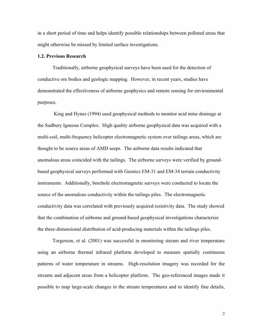
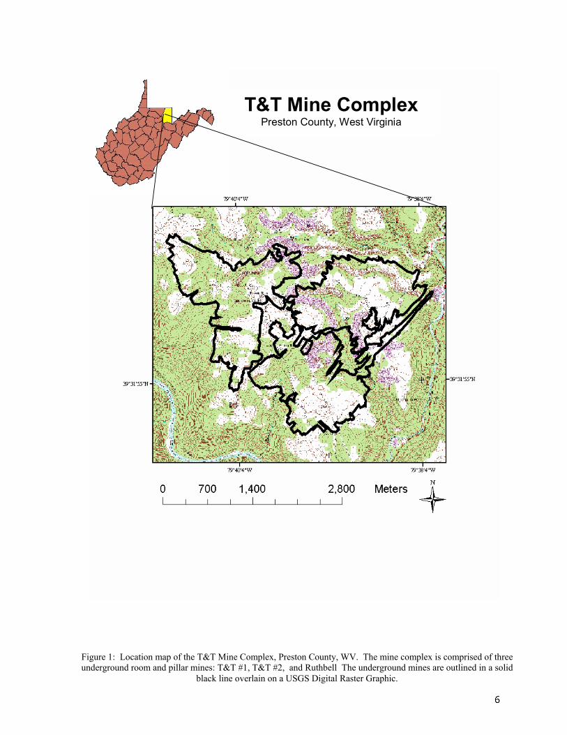
Figure 1: Location map of the T&T Mine Complex, Preston County, WV. The mine complex is comprised of threeunderground room and pillar mines: T&T #1, T&T #2, and Ruthbell The underground mines are outlined in a solid

black line overlain on a USGS Digital Raster Graphic.

T&T Mine Complex Preston County, West Virginia

7

1.4. Site Description

The T&T Mine Complex is located in near Albright, Preston County, West Virginia

(Figure 1). The complex is comprised of three underground, room and pillar mines: T&T #1,

T&T #2, and the Ruthbell Mine. The mines are situated in the Pennsylvanian Conemaugh

Group and Allegheny Formation, and are located at a depth approximately 85-90 meters

below the surface. The target coal seam was the Upper Freeport Coal, a multiple-bedded

coal seam ranging in thickness from 0 to 3 meters, and marks the boundary between the

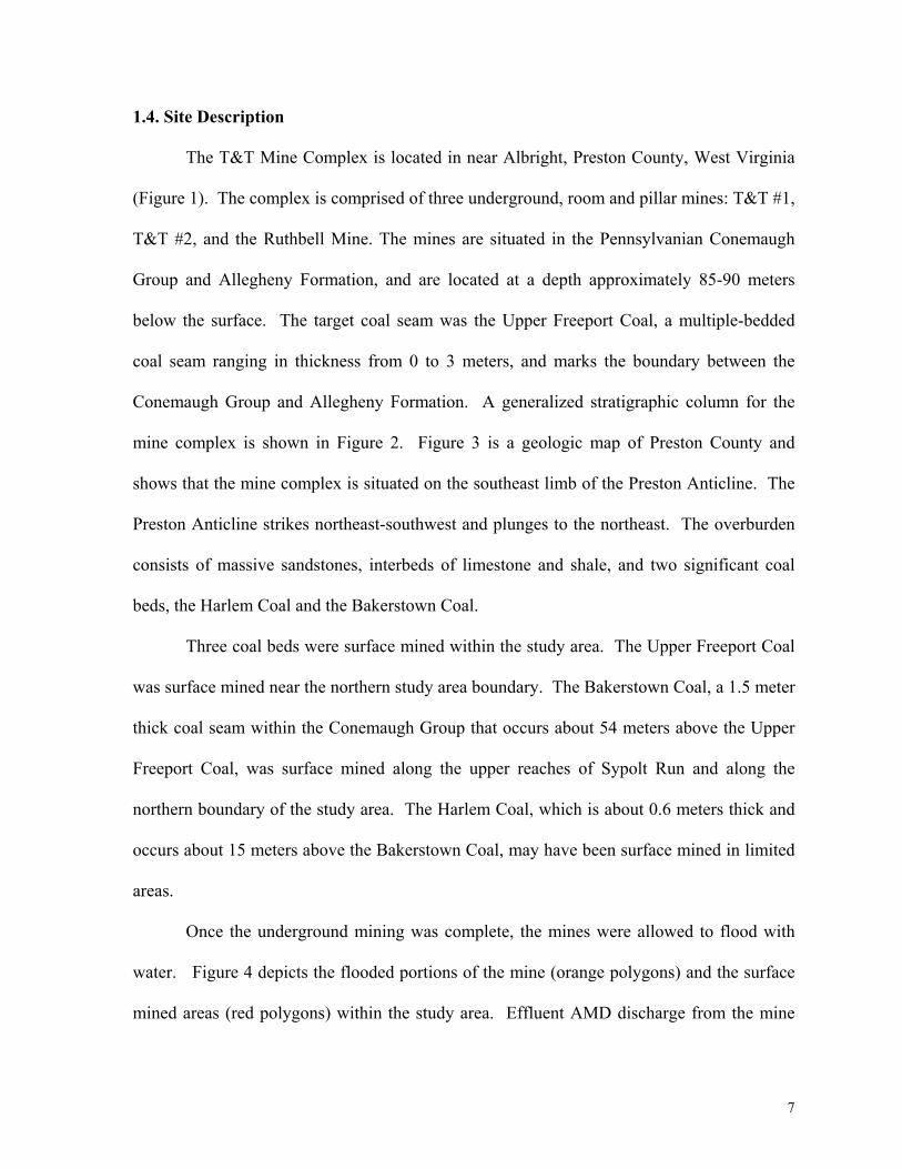
Conemaugh Group and Allegheny Formation. A generalized stratigraphic column for the

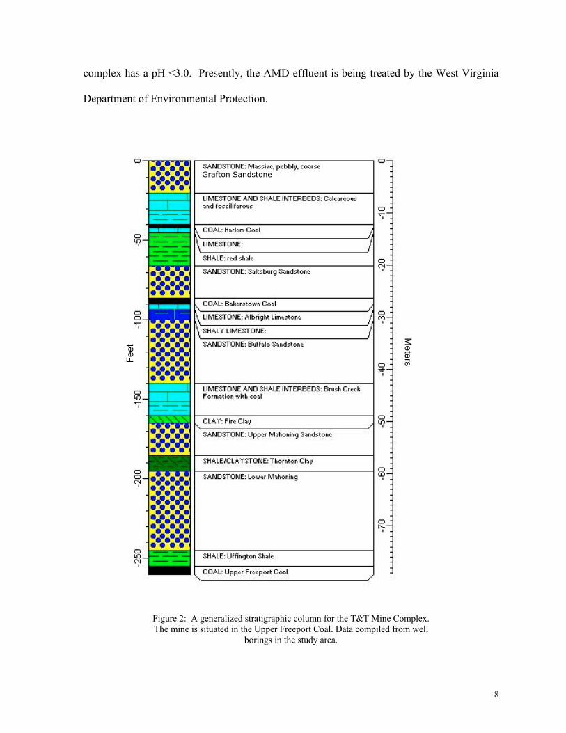
mine complex is shown in Figure 2. Figure 3 is a geologic map of Preston County and

shows that the mine complex is situated on the southeast limb of the Preston Anticline. The

Preston Anticline strikes northeast-southwest and plunges to the northeast. The overburden

consists of massive sandstones, interbeds of limestone and shale, and two significant coal

beds, the Harlem Coal and the Bakerstown Coal.

Three coal beds were surface mined within the study area. The Upper Freeport Coal

was surface mined near the northern study area boundary. The Bakerstown Coal, a 1.5 meter

thick coal seam within the Conemaugh Group that occurs about 54 meters above the Upper

Freeport Coal, was surface mined along the upper reaches of Sypolt Run and along the

northern boundary of the study area. The Harlem Coal, which is about 0.6 meters thick and

occurs about 15 meters above the Bakerstown Coal, may have been surface mined in limited

areas.

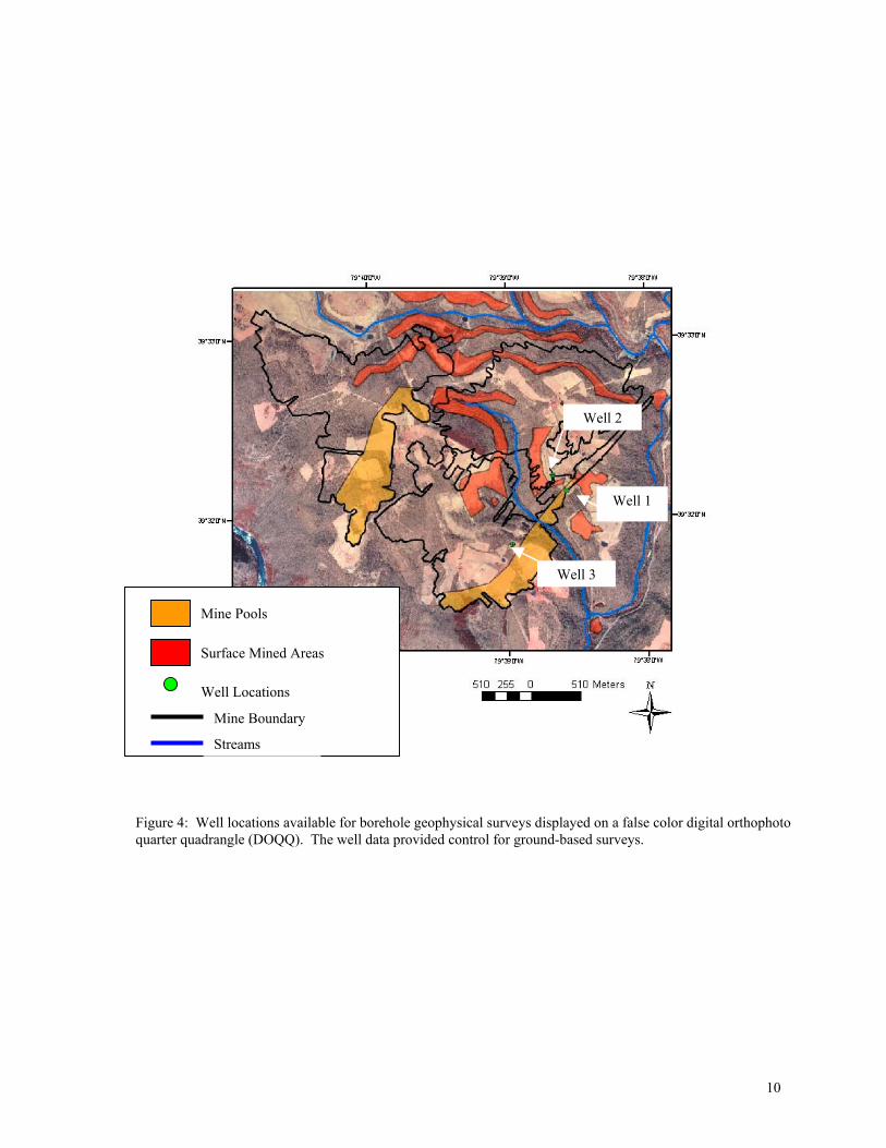
Once the underground mining was complete, the mines were allowed to flood with

water. Figure 4 depicts the flooded portions of the mine (orange polygons) and the surface

mined areas (red polygons) within the study area. Effluent AMD discharge from the mine

8

complex has a pH <3.0. Presently, the AMD effluent is being treated by the West Virginia

Department of Environmental Protection.

Feet

Meters

Figure 2: A generalized stratigraphic column for the T&T Mine Complex.The mine is situated in the Upper Freeport Coal. Data compiled from well

borings in the study area.

Grafton Sandstone

9

Figure 3: Geologic map of study area. The mine complex is situated on the southeast limb of the Prestonanticline.

Legend

Preston Anticline

Kingwood Syncline

Mine Boundary

Alluvium

Monongalia Series

Conemaugh Series

Allegheny Series

Pottsville Series

Mauch Chunk Series

Greenbrier Series

Pocono Series

Catskill Series

Chemung Series

Alluvium

Monongalia Series

Conemaugh Series

Allegheny Series

Pottsville Series

Mauch Chunk Series

Greenbrier Series

Pocono Series

Catskill Series

Alluvium

Monongalia Series

Conemaugh Series

Allegheny Series

Pottsville Series

Mauch Chunk Series

Greenbrier Series

Pocono Series

Alluvium

Monongalia Series

Conemaugh Series

Allegheny Series

Pottsville Series

Mauch Chunk Series

Greenbrier Series

Alluvium

Monongalia Series

Conemaugh Series

Allegheny Series

Pottsville Series

Mauch Chunk Series

Alluvium

Monongalia Series

Conemaugh Series

Allegheny Series

Pottsville Series

Alluvium

Monongalia Series

Conemaugh Series

Allegheny Series

Alluvium

Monongalia Series

Conemaugh Series

Alluvium

Monongalia Series

AlluviumAlluvium

Monongalia Series

Conemaugh Series

Allegheny SeriesAllegheny Series

Pottsville SeriesPottsville Series

Mauch Chunk SeriesMauch Chunk Series

Greenbrier SeriesGreenbrier Series

Pocono Series

Catskill Series

Chemung Series

10

Mine Pools

Surface Mined Areas

Well Locations

Streams

Mine Boundary

Well 1

Well 2

Well 3

Figure 4: Well locations available for borehole geophysical surveys displayed on a false color digital orthophotoquarter quadrangle (DOQQ). The well data provided control for ground-based surveys.

11

CHAPTER 2 – Review of Geophysical and Remote Sensing Methods forEnvironmental Applications

2.1. Terrain Conductivity

Conductivity varies within the earth and is controlled by the rocks and soil that make

up the subsurface. Factors controlling the conductivity of a given area are: porosity,

moisture content, dissolved electrolyte content, temperature and phase state of pore water,

and the amount and composition of colloids (McNeill, 1980-a).

The terrain conductivity method uses a transmitter coil that produces a primary

electromagnetic wave that travels through the ground. The alternating electric current

produces an alternating magnetic field that induces current flow through the earth. Current

flow in the receiver coil is induced in response to the electromagnetic fields generated by the

transmitter and the induced secondary ground currents.

The strength of the secondary field is dependent on intercoil spacing, frequency of

the primary field, and ground conductivity. As described by McNeill, there is a simple

relationship between the primary and secondary fields when the operation frequency of the

terrain conductivity meter is confined to the constraints of a low induction number. The

terrain conductivity has a linear relationship with the ratio of the primary and secondary

magnetic fields. McNeill (1980-b) gives the relationship:

Hs = iωµ0σs2

Hp 4

Where Hs is the secondary magnetic field at the receiver coil

Hp is the primary magnetic field at the receiver coil

ω is equal to 2πf

(1)

12

f is the frequency of alternating current in transmitter coil

µ0 is permeability of free space

σ is ground conductivity

s is the intercoil spacing

i is square root of -1.

The instrument directly measures the primary and secondary fields and the ratio is known;

therefore, the apparent conductivity is also known (McNeill, 1980-b).

A low induction number makes the general relationship between the ratio of the

primary and secondary and terrain conductivity possible. The induction number, B, is

dependent on the intercoil spacing and the skin depth:

B = s δ

Where s is the intercoil spacing and δ is the skin depth (McNeill, 1980-b). The skin depth is

described as the depth at which the amplitude of the electromagnetic field drops to 1/e of the

source amplitude (e being the natural base). Skin depth is a function of the operating

frequency and the ground conductivity (McNeill, 1980). The skin depth is given by the

following relationship:

δ = 500(1/σf)1/2

As implied by this relationship, increases in ground conductivity and frequency will decrease

the skin depth, and therefore, decrease the depth of investigation.

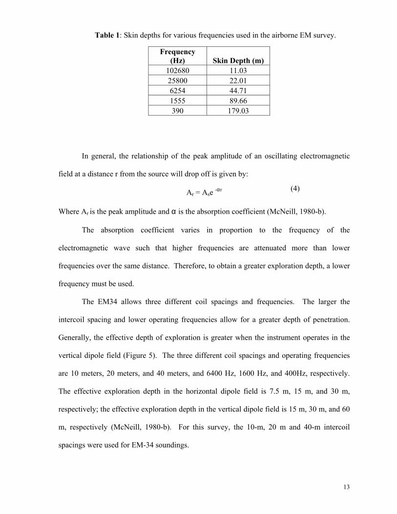
The average conductivity, as calculated from the induction logs at the mine complex,

is approximately 20 millimhos per meter (mmhos/m). Using equation 3, the skin depths for

the various airborne frequencies were calculated (Table 1).

(3)

(2)

13

Frequency(Hz) Skin Depth (m)

102680 11.0325800 22.016254 44.711555 89.66390 179.03

In general, the relationship of the peak amplitude of an oscillating electromagnetic

field at a distance r from the source will drop off is given by:

Ar = Ase -αr

Where Ar is the peak amplitude and α is the absorption coefficient (McNeill, 1980-b).

The absorption coefficient varies in proportion to the frequency of the

electromagnetic wave such that higher frequencies are attenuated more than lower

frequencies over the same distance. Therefore, to obtain a greater exploration depth, a lower

frequency must be used.

The EM34 allows three different coil spacings and frequencies. The larger the

intercoil spacing and lower operating frequencies allow for a greater depth of penetration.

Generally, the effective depth of exploration is greater when the instrument operates in the

vertical dipole field (Figure 5). The three different coil spacings and operating frequencies

are 10 meters, 20 meters, and 40 meters, and 6400 Hz, 1600 Hz, and 400Hz, respectively.

The effective exploration depth in the horizontal dipole field is 7.5 m, 15 m, and 30 m,

respectively; the effective exploration depth in the vertical dipole field is 15 m, 30 m, and 60

m, respectively (McNeill, 1980-b). For this survey, the 10-m, 20 m and 40-m intercoil

spacings were used for EM-34 soundings.

(4)

Table 1: Skin depths for various frequencies used in the airborne EM survey.

14

The apparent conductivity measured at the surface by the conductivity meter is a

composite response of the contributions from the entire subsurface medium. The relative

contribution of a given interval at arbitrary depths to measure terrain conductivity is defined

by the relative response function Φ(z), where z is the depth divided by the intercoil spacing

and Φ(z) quantifies the relative contribution to the secondary magnetic field arising from a

thin layer at any depth z (McNeill, 1980-b). Figure 6 depicts the relative response function

for the vertical and horizontal dipole modes of operation. Note how each dipole responds to

materials at depth. The horizontal dipole is much more sensitive to near surface materials

and drops off significantly at depth. The vertical dipole exhibits little or no response to near

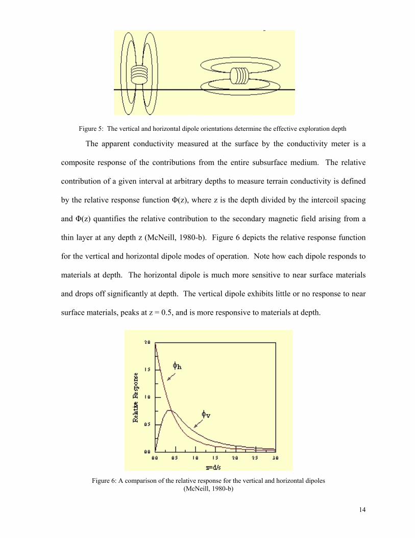
surface materials, peaks at z = 0.5, and is more responsive to materials at depth.

Figure 5: The vertical and horizontal dipole orientations determine the effective exploration depth

Figure 6: A comparison of the relative response for the vertical and horizontal dipoles(McNeill, 1980-b)

15

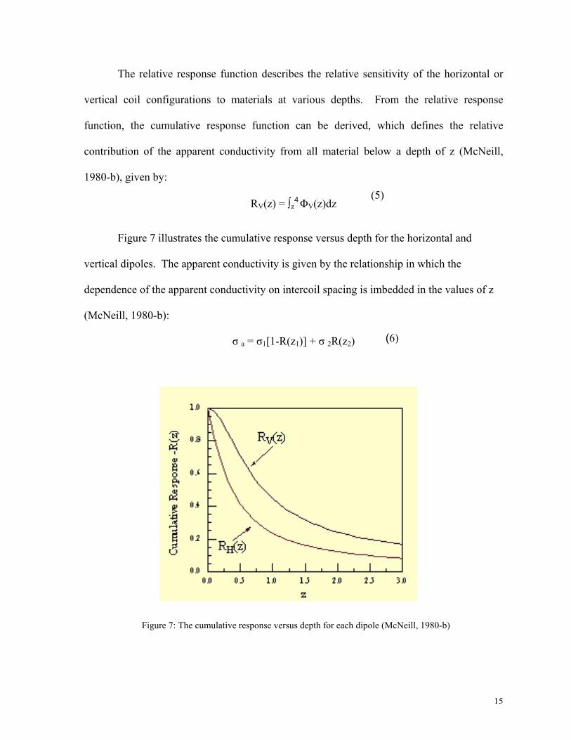
Figure 7: The cumulative response versus depth for each dipole (McNeill, 1980-b)

The relative response function describes the relative sensitivity of the horizontal or

vertical coil configurations to materials at various depths. From the relative response

function, the cumulative response function can be derived, which defines the relative

contribution of the apparent conductivity from all material below a depth of z (McNeill,

1980-b), given by:

RV(z) = ∫z4 ΦV(z)dz

Figure 7 illustrates the cumulative response versus depth for the horizontal and

vertical dipoles. The apparent conductivity is given by the relationship in which the

dependence of the apparent conductivity on intercoil spacing is imbedded in the values of z

(McNeill, 1980-b):

σ a = σ1[1-R(z1)] + σ 2R(z2)

(5)

(6)

16

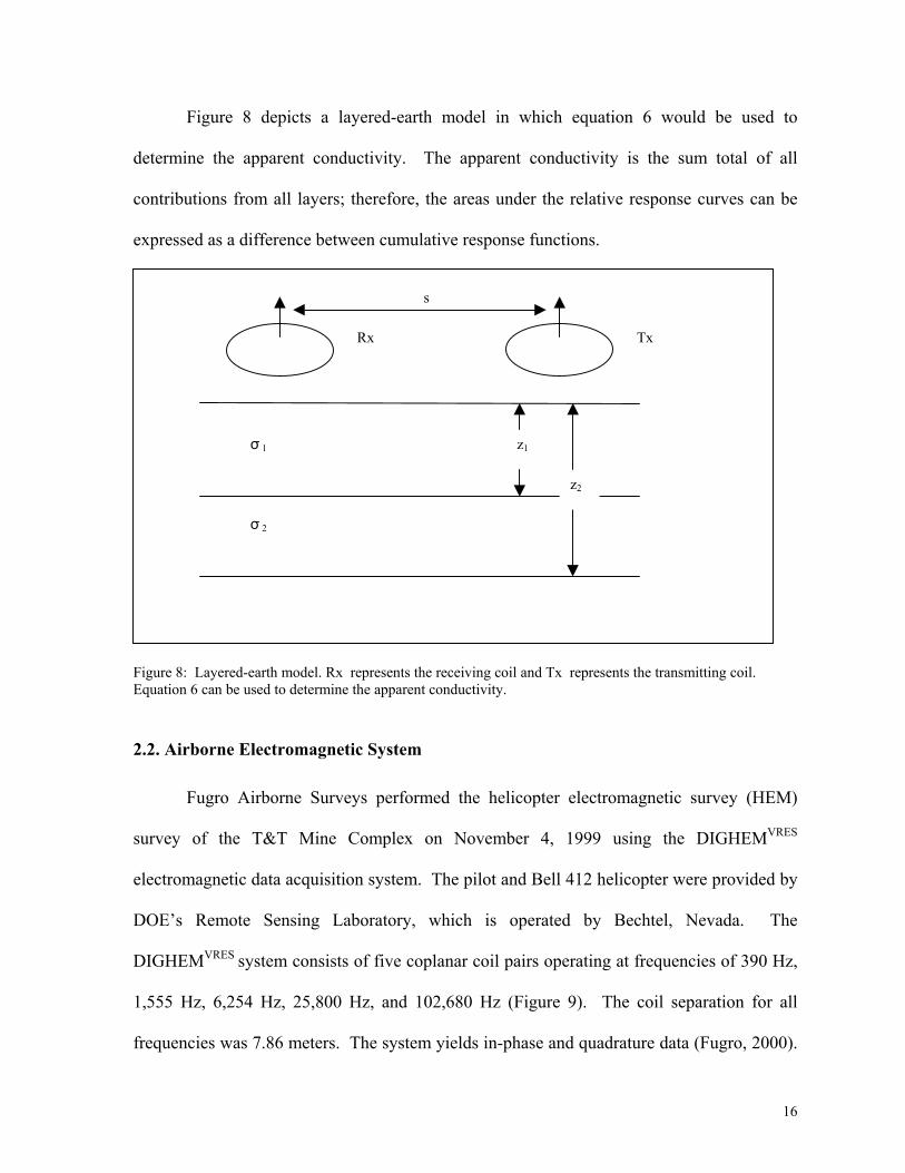
Figure 8 depicts a layered-earth model in which equation 6 would be used to

determine the apparent conductivity. The apparent conductivity is the sum total of all

contributions from all layers; therefore, the areas under the relative response curves can be

expressed as a difference between cumulative response functions.

Figure 8: Layered-earth model. Rx represents the receiving coil and Tx represents the transmitting coil.Equation 6 can be used to determine the apparent conductivity.

2.2. Airborne Electromagnetic System

Fugro Airborne Surveys performed the helicopter electromagnetic survey (HEM)

survey of the T&T Mine Complex on November 4, 1999 using the DIGHEMVRES

electromagnetic data acquisition system. The pilot and Bell 412 helicopter were provided by

DOE’s Remote Sensing Laboratory, which is operated by Bechtel, Nevada. The

DIGHEMVRES system consists of five coplanar coil pairs operating at frequencies of 390 Hz,

1,555 Hz, 6,254 Hz, 25,800 Hz, and 102,680 Hz (Figure 9). The coil separation for all

frequencies was 7.86 meters. The system yields in-phase and quadrature data (Fugro, 2000).

s

Rx Tx

z1

z2

σ 1

σ 2

17

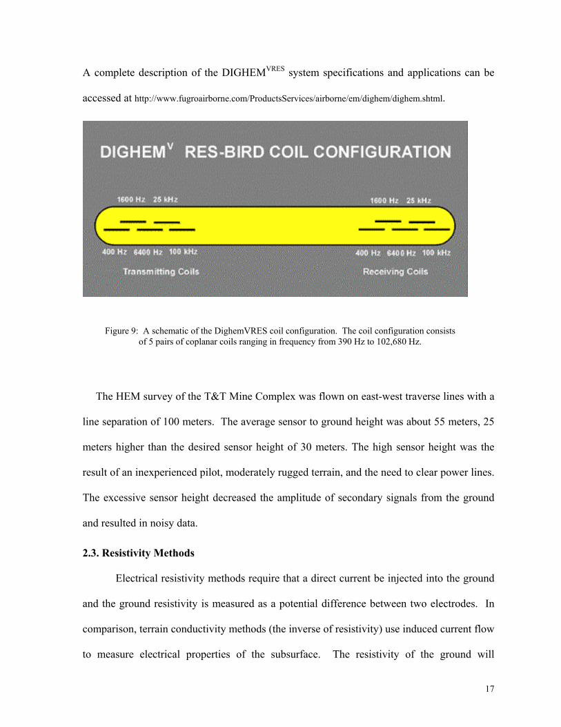
A complete description of the DIGHEMVRES system specifications and applications can be

accessed at http://www.fugroairborne.com/ProductsServices/airborne/em/dighem/dighem.shtml.

The HEM survey of the T&T Mine Complex was flown on east-west traverse lines with a

line separation of 100 meters. The average sensor to ground height was about 55 meters, 25

meters higher than the desired sensor height of 30 meters. The high sensor height was the

result of an inexperienced pilot, moderately rugged terrain, and the need to clear power lines.

The excessive sensor height decreased the amplitude of secondary signals from the ground

and resulted in noisy data.

2.3. Resistivity Methods

Electrical resistivity methods require that a direct current be injected into the ground

and the ground resistivity is measured as a potential difference between two electrodes. In

comparison, terrain conductivity methods (the inverse of resistivity) use induced current flow

to measure electrical properties of the subsurface. The resistivity of the ground will

Figure 9: A schematic of the DighemVRES coil configuration. The coil configuration consistsof 5 pairs of coplanar coils ranging in frequency from 390 Hz to 102,680 Hz.

18

correspond to true resistivity if the ground is homogenous and isotropic (Yazicigil and

Sendlein, 1982). However, this is seldom the case. The measured resistivity is apparent

resistivity, given by the equation (Burger, 1992):

ρ = 2πV (1 – 1 – 1 + 1)-1

i d1 d 2 d 3 d 4 (7)

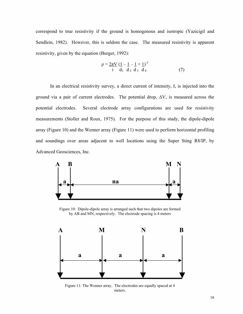
In an electrical resistivity survey, a direct current of intensity, I, is injected into the

ground via a pair of current electrodes. The potential drop, ∆V, is measured across the

potential electrodes. Several electrode array configurations are used for resistivity

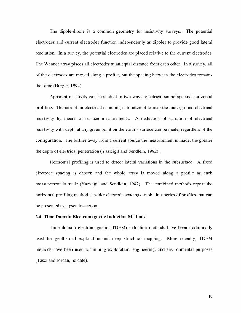
measurements (Stoller and Roux, 1975). For the purpose of this study, the dipole-dipole

array (Figure 10) and the Wenner array (Figure 11) were used to perform horizontal profiling

and soundings over areas adjacent to well locations using the Super Sting R8/IP, by

Advanced Geosciences, Inc.

a ana

A B M N

Figure 10: Dipole-dipole array is arranged such that two dipoles are formedby AB and MN, respectively. The electrode spacing is 4 meters

a a a

A M N B

Figure 11: The Wenner array. The electrodes are equally spaced at 4meters.

19

The dipole-dipole is a common geometry for resistivity surveys. The potential

electrodes and current electrodes function independently as dipoles to provide good lateral

resolution. In a survey, the potential electrodes are placed relative to the current electrodes.

The Wenner array places all electrodes at an equal distance from each other. In a survey, all

of the electrodes are moved along a profile, but the spacing between the electrodes remains

the same (Burger, 1992).

Apparent resistivity can be studied in two ways: electrical soundings and horizontal

profiling. The aim of an electrical sounding is to attempt to map the underground electrical

resistivity by means of surface measurements. A deduction of variation of electrical

resistivity with depth at any given point on the earth’s surface can be made, regardless of the

configuration. The further away from a current source the measurement is made, the greater

the depth of electrical penetration (Yazicigil and Sendlein, 1982).

Horizontal profiling is used to detect lateral variations in the subsurface. A fixed

electrode spacing is chosen and the whole array is moved along a profile as each

measurement is made (Yazicigil and Sendlein, 1982). The combined methods repeat the

horizontal profiling method at wider electrode spacings to obtain a series of profiles that can

be presented as a pseudo-section.

2.4. Time Domain Electromagnetic Induction Methods

Time domain electromagnetic (TDEM) induction methods have been traditionally

used for geothermal exploration and deep structural mapping. More recently, TDEM

methods have been used for mining exploration, engineering, and environmental purposes

(Tasci and Jordan, no date).

20

TDEM methods are those in which time-dependent magnetic fields are created by

inducing square waves of current through a grounded wire source. Passing a step current

through the cable generates an electromagnetic field. There are two parts to this magnetic

field; one from the current flowing through the cable, and the other from the return currents

flowing through the Earth (Keller, 1997).

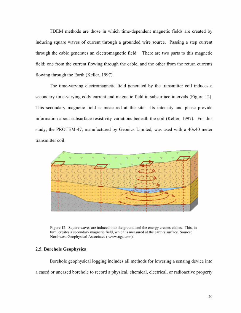
The time-varying electromagnetic field generated by the transmitter coil induces a

secondary time-varying eddy current and magnetic field in subsurface intervals (Figure 12).

This secondary magnetic field is measured at the site. Its intensity and phase provide

information about subsurface resistivity variations beneath the coil (Keller, 1997). For this

study, the PROTEM-47, manufactured by Geonics Limited, was used with a 40x40 meter

transmitter coil.

2.5. Borehole Geophysics

Borehole geophysical logging includes all methods for lowering a sensing device into

a cased or uncased borehole to record a physical, chemical, electrical, or radioactive property

Figure 12: Square waves are induced into the ground and the energy creates eddies. This, inturn, creates a secondary magnetic field, which is measured at the earth’s surface. Source:Northwest Geophysical Associates ( www.nga.com).

21

along the well bore. Traditionally used by the petroleum industry, the properties useful for

determining oil and gas prospects can also be used in environmental and hydrological

investigations associated with ground water pollution.

Three wells on the study site were available for borehole geophysics (see Figure 4).

Each well was drilled into a known mine void by Coastal Coal Company in order to inject a

neutralizing lime slurry into the flooded portion of the underground mine. The mine is

situated on the east limb of a plunging anticline; the wells were drilled up-gradient of

inferred mine pools for the lime slurry injection. Each well was drilled to an approximate

depth of 80 meters below the surface. The suite of geophysical logs completed in each well

includes an induction log to measure electrical conductivity, and neutron, natural gamma,

and gamma-gamma logs.

Neutron logs use a radioactive source that releases neutrons into a formation. The

neutrons cause formations to emit gamma rays which are proportional to hydrogen content.

The gamma radiation is recorded by the logging instrument. Neutron logs are often used to

determine porosity, water content, and moisture content within a formation (Keys, 1988).

Natural gamma logs record the amount of naturally occurring gamma radiation in the

borehole vicinity. Clay-bearing rocks naturally emit a high amount of gamma radiation due

the abundance of potassium in clays and micas (Keys, 1988).

The gamma-gamma log, or density log, measures density through gamma radiation.

The logging tool emits gamma radiation and records the amount of gamma radiation that

returns from the formation surrounding the borehole area (Keys, 1988). The logs are

calibrated such that bulk density is calculated.

22

2.6. Thermal Infrared Imagery

Temperature can be described two ways: kinetic temperature or radiant

temperature. Kinetic temperature is the internal manifestation of the average energy of the

molecules which make up the body. Radiant temperature can be described as an object’s

external manifestation of molecular energy states. It is the external manifestation of an

object’s energy state that is remotely sensed (Lillesand and Kiefer, 2000).

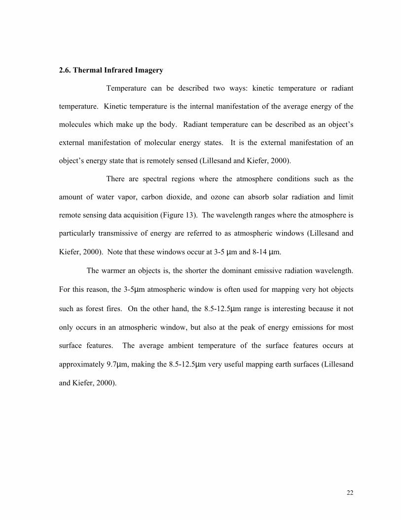
There are spectral regions where the atmosphere conditions such as the

amount of water vapor, carbon dioxide, and ozone can absorb solar radiation and limit

remote sensing data acquisition (Figure 13). The wavelength ranges where the atmosphere is

particularly transmissive of energy are referred to as atmospheric windows (Lillesand and

Kiefer, 2000). Note that these windows occur at 3-5 µm and 8-14 µm.

The warmer an objects is, the shorter the dominant emissive radiation wavelength.

For this reason, the 3-5µm atmospheric window is often used for mapping very hot objects

such as forest fires. On the other hand, the 8.5-12.5µm range is interesting because it not

only occurs in an atmospheric window, but also at the peak of energy emissions for most

surface features. The average ambient temperature of the surface features occurs at

approximately 9.7µm, making the 8.5-12.5µm very useful mapping earth surfaces (Lillesand

and Kiefer, 2000).

23

0 4 8 12 16 20 24

Midnight MidnightNoon

Rad

iant

Tem

pera

ture

DAW

N SUN

SET

Water

Soils and Rocks

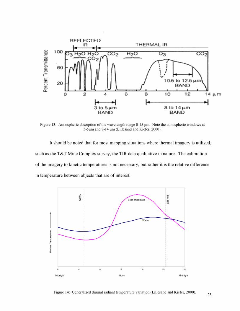
Figure 14: Generalized diurnal radiant temperature variation (Lillesand and Kiefer, 2000).

It should be noted that for most mapping situations where thermal imagery is utilized,

such as the T&T Mine Complex survey, the TIR data qualitative in nature. The calibration

of the imagery to kinetic temperatures is not necessary, but rather it is the relative difference

in temperature between objects that are of interest.

Figure 13: Atmospheric absorption of the wavelength range 0-15 µm. Note the atmospheric windows at3-5µm and 8-14 µm (Lillesand and Kiefer, 2000).

24

Diurnal variations must be considered when acquiring thermal data. The comparison

between the diurnal temperatures of water with that of soils and rock is shown in Figure 14.

Note that the highest contrast between the ground and water occurs a few hours past solar

noon and cooling takes place thereafter. Nighttime imagery is preferred because daylight

data is dominated by variations in solar heating due to topography. The temperature curve

for water is quite distinctive because the diurnal temperature range of water is very small

compared to the ground temperature range, and water reaches its maximum temperature at a

delayed time compared to the other materials. It can be concluded from the graph that the

ground surface temperature is higher during the day and lower during the night than water

temperature. The two points where the line crosses are called crossovers and they indicate

no difference between the ground surface temperature and the water temperatures (Lillesand

and Kiefer, 2000).

Two channels of nighttime thermal infrared imagery (TIR) were acquired at the T&T

Mine Complex as part of a survey of the Muddy Creek/Roaring Creek Watershed. The

thermal sensor was a Daedalus AADS 1268 multi-spectral line scanner (MSS) coupled to a

position and orientation system (POS). The MSS was configured for nighttime thermal

operation with a spectral sensitivity range of 3-5µm (band 1) and 8.5-12.5µm (band 2). A

GPS navigation system was used to plot the planned survey route. A minimum 30% overlap

was specified between adjacent flight lines. The POS consisted of a Litton LN-200 inertial

measurement unit (IMU), which provided trajectory data that was used to record orientation

of the sensor head on the MSS. This instrument configuration allows data to be geo-rectified

for distortions brought about by aircraft attitude (pitch, roll, and yaw) (Brewster, 1999). The

25

data is corrected for geometric distortion using a combination of inertial measurements and

Differential Global Positioning System (DGPS) navigation data collected in the air. The final

corrected positional accuracy was found to be approximately ± 1 meter. The data were also

radiometrically corrected.

The thermal data were acquired between 3:00 am and 6:00 am to ensure optimal

thermal contrast between cold surface water and warmer ground water from mine discharges,

seeps, and springs. This time window allows objects heated by sunlight during the day to

reach temperature equilibrium with the surroundings.

26

CHAPTER 3 – Modeling Results and Discussion

3.1. Borehole Geophysics

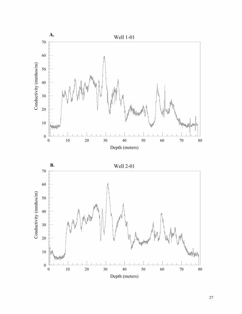
Three wells were available to perform borehole geophysical surveys. The suite of

geophysical logs completed in each well included induction, gamma-gamma, natural gamma,

and neutron. The results of the induction logs are shown in Figure 15. In order to determine

a starting model for the terrain conductivity modeling, the induction logs were averaged into

geoelectric layers, which are not necessarily geologic layers (Keller and Frischknecht, 1966).

As defined by Keller and Frischknecht (1966), a geoelectric layer is bounded by changes in

electrical properties of the rocks and can contain many geologic layers or reside inside a

single geologic layer. The geoelectric layered models contain layers of relatively similar

electrical conductivity, not constant geology as the geology is more complicated than models

in this project can represent.

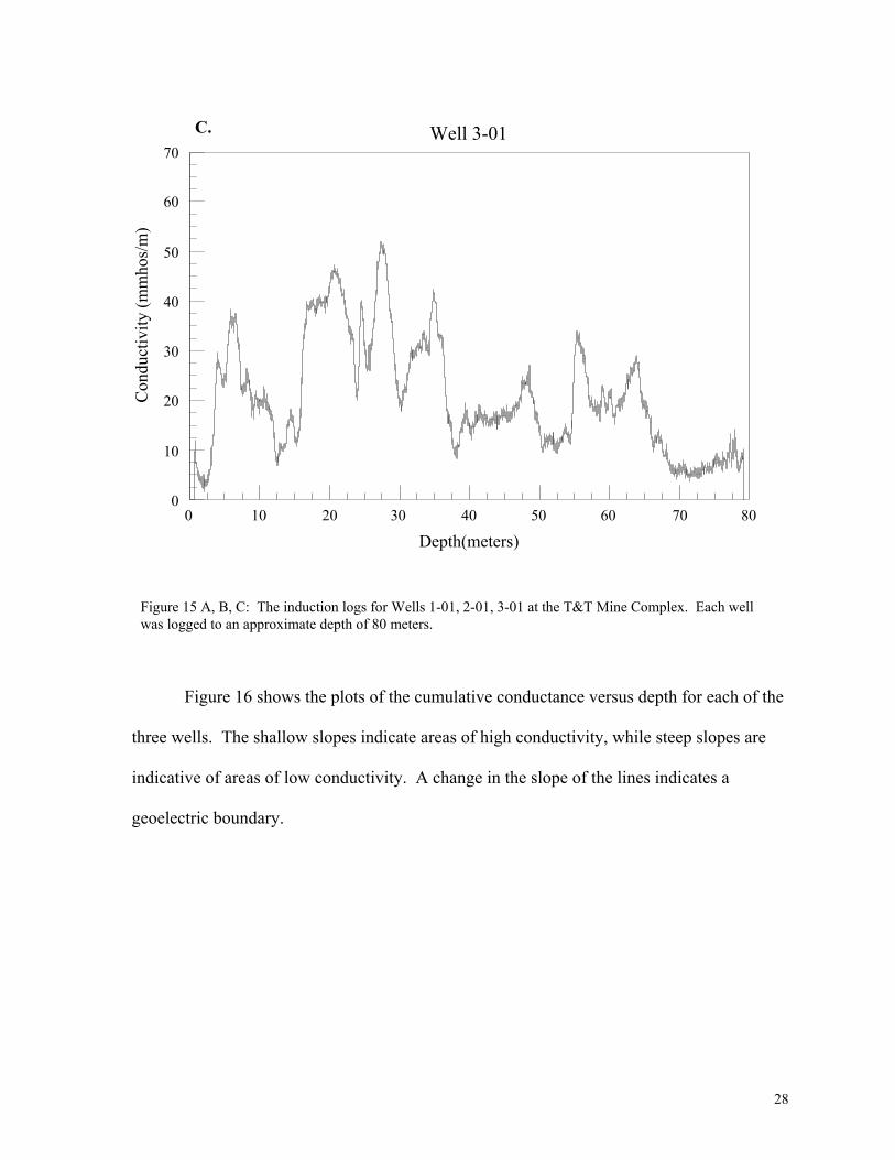
The results of the induction logs are blocked into intervals of similar conductivity. In

order to determine where boundaries should be placed to make a multi-layered conductivity

model, the cumulative conductance is calculated and plotted against depth for each well

(Stoyer, 1998). Cumulative conductance is calculated by summing the longitudinal

conductance of each of the many thin layers from the well log and is calculated by dividing

resistance (ρ) of each layer by layer thickness (h):

S cum = ∑ hi/ρi(8)

27

Depth (meters)0 10 20 30 40 50 60 70 80

Con

duct

ivity

(mm

hos/

m)

0

10

20

30

40

50

60

70Well 1-01A.

Depth (meters)0 10 20 30 40 50 60 70 80

Con

duct

ivity

(mm

hos/

m)

0

10

20

30

40

50

60

70Well 2-01B.

28

Depth(meters)0 10 20 30 40 50 60 70 80

Con

duct

ivity

(mm

hos/

m)

0

10

20

30

40

50

60

70Well 3-01C.

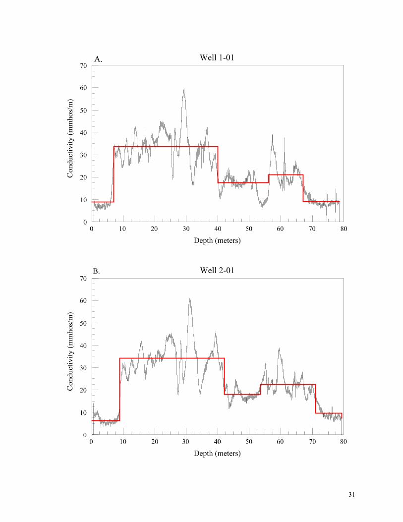
Figure 16 shows the plots of the cumulative conductance versus depth for each of the

three wells. The shallow slopes indicate areas of high conductivity, while steep slopes are

indicative of areas of low conductivity. A change in the slope of the lines indicates a

geoelectric boundary.

Figure 15 A, B, C: The induction logs for Wells 1-01, 2-01, 3-01 at the T&T Mine Complex. Each wellwas logged to an approximate depth of 80 meters.

29

Cumulative Conductance0.00 0.50 1.00 1.50 2.00

Dep

th (m

eter

s)0

10

20

30

40

50

60

70

80

Well 1-01Layer 1

Layer 2

Layer 3

Layer 4

Layer 5

A.

Cumulative Conductance0.00 0.50 1.00 1.50 2.00

Dep

th (m

eter

s)

0

10

20

30

40

50

60

70

80

Well 2-01

Layer 1

Layer 2

Layer 3

Layer 4

Layer 5

B.

30

Cumulative Conductance0.00 0.50 1.00 1.50 2.00

Dep

th(m

eter

s)0

10

20

30

40

50

60

70

80

Well 3-01C.Layer 1

Layer 2

Layer 3

Layer 4

Layer 5

Layer 6

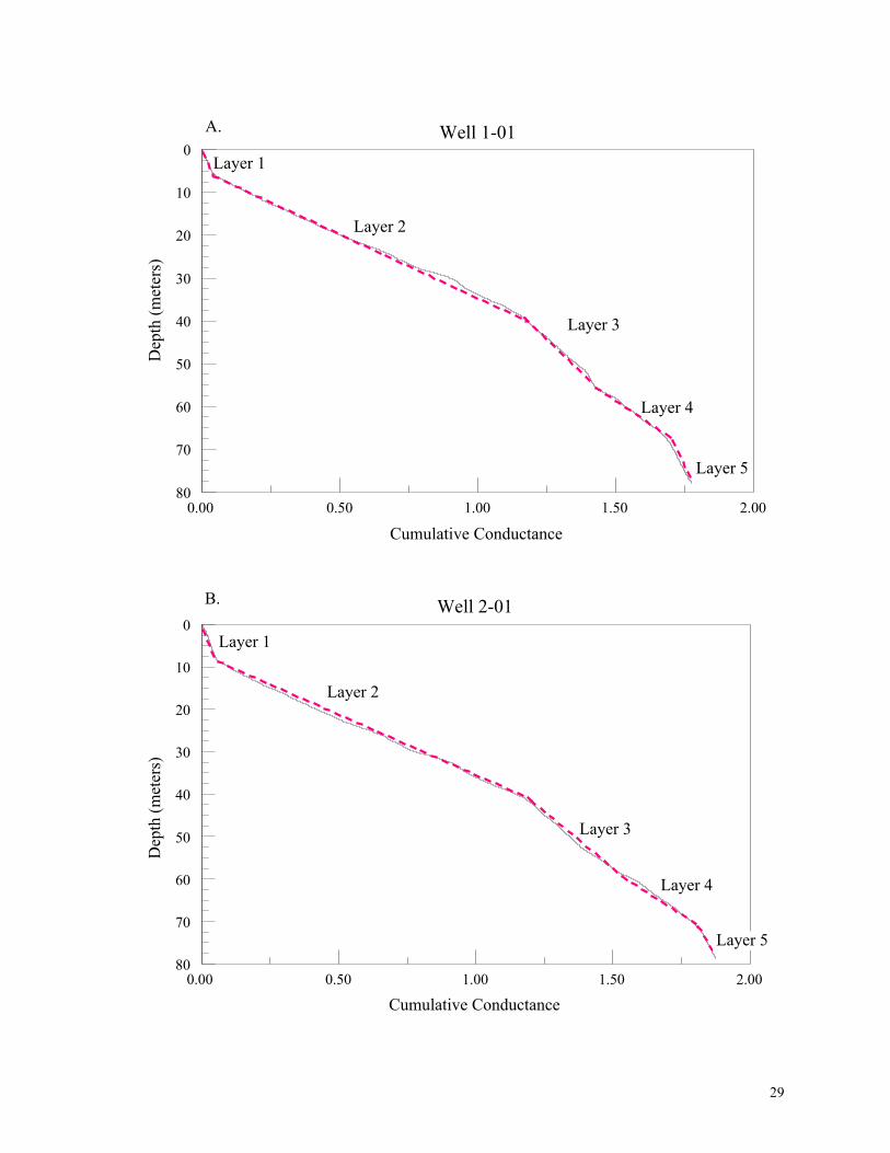
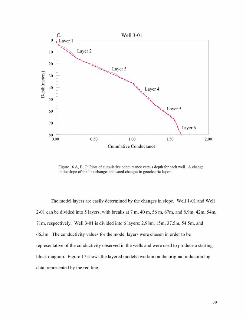
The model layers are easily determined by the changes in slope. Well 1-01 and Well

2-01 can be divided into 5 layers, with breaks at 7 m, 40 m, 56 m, 67m, and 8.9m, 42m, 54m,

71m, respectively. Well 3-01 is divided into 6 layers: 2.98m, 15m, 37.5m, 54.5m, and

66.3m. The conductivity values for the model layers were chosen in order to be

representative of the conductivity observed in the wells and were used to produce a starting

block diagram. Figure 17 shows the layered models overlain on the original induction log

data, represented by the red line.

Figure 16 A, B, C: Plots of cumulative conductance versus depth for each well. A changein the slope of the line changes indicated changes in geoelectric layers.

31

Depth (meters)0 10 20 30 40 50 60 70 80

Con

duct

ivity

(mm

hos/

m)

0

10

20

30

40

50

60

70Well 1-01A.

Depth (meters)0 10 20 30 40 50 60 70 80

Con

duct

ivity

(mm

hos/

m)

0

10

20

30

40

50

60

70Well 2-01B.

32

Depth(meters)0 10 20 30 40 50 60 70 80

Con

duct

ivity

(mm

hos/

m)

0

10

20

30

40

50

60

70Well 3-01C.

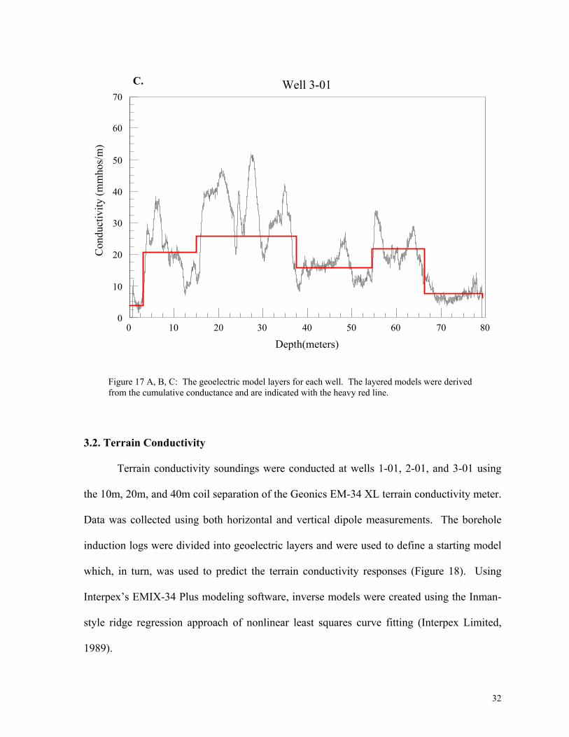
3.2. Terrain Conductivity

Terrain conductivity soundings were conducted at wells 1-01, 2-01, and 3-01 using

the 10m, 20m, and 40m coil separation of the Geonics EM-34 XL terrain conductivity meter.

Data was collected using both horizontal and vertical dipole measurements. The borehole

induction logs were divided into geoelectric layers and were used to define a starting model

which, in turn, was used to predict the terrain conductivity responses (Figure 18). Using

Interpex’s EMIX-34 Plus modeling software, inverse models were created using the Inman-

style ridge regression approach of nonlinear least squares curve fitting (Interpex Limited,

1989).

Figure 17 A, B, C: The geoelectric model layers for each well. The layered models were derivedfrom the cumulative conductance and are indicated with the heavy red line.

33

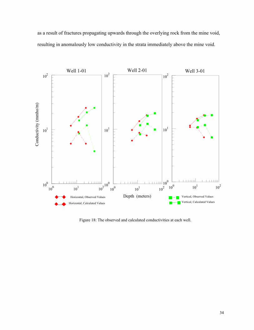
Figure 18 is a graphical representation of the field observations and calculated

conductivities from the starting model for three intercoil spacings. These three-point

soundings consist of measurements made at the 10, 20, and 40 meter intercoil spacings. For

each sounding, the calculated and observed data show similar increasing values at the 10 m

and 20 m coil separation; however, at the 40 m intercoil spacing, the match between the

observed and calculated data drops off significantly. Models were generated in order to

investigate possible ways in which these differences could be explained and to minimize the

great disparity between the calculated and observed data.

The simplified induction logs (Figure 17) served as starting models for the forward

and inverse modeling process. In the modeling effort, the thickness of layers observed in the

borehole remained fixed during the inversion; only layer conductivity was allowed to vary,

meaning that the values of layer conductivity parameters could be varied during the

inversion process to minimize differences between the calculated response and field

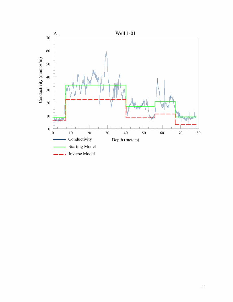
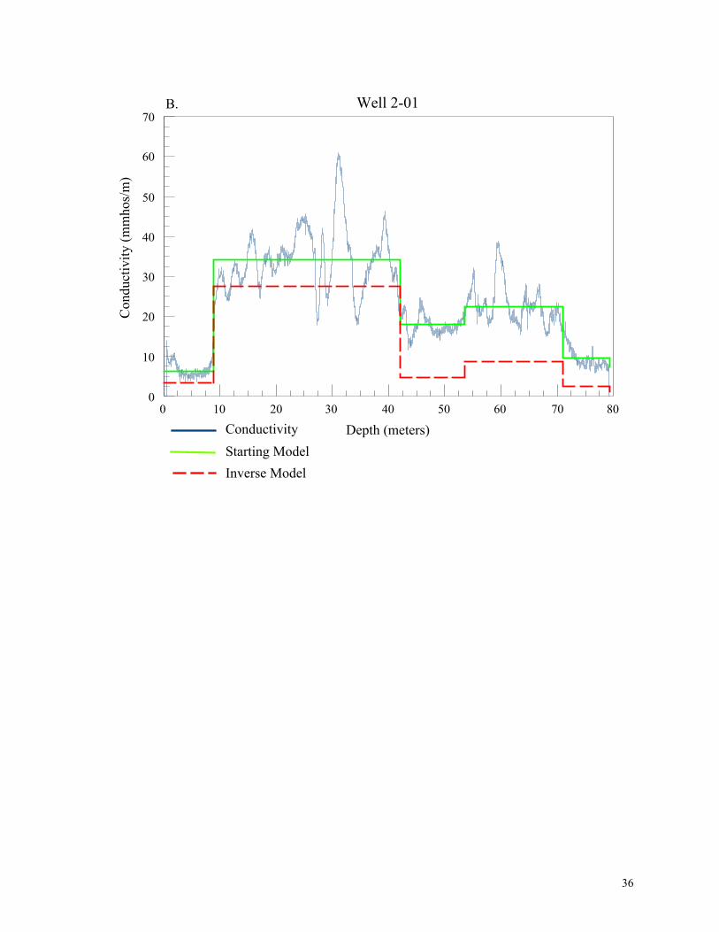
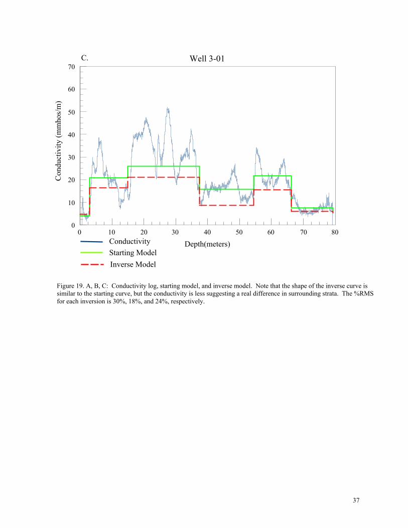
observations. Inverse models are shown in Figure 19 A-C. Notice that the general

conductivities derived by modeling are similar to the conductivities portrayed in the initial

starting models. However, the layer conductivities derived by inversion are lower than those

observed in the wells logs. The calculated and observed conductivities for the inverse model

are shown in Figure 20. The anomalously low apparent conductivity observed at the 40-

meter coil separation suggests the presence of a real difference between the conductivity in

the immediate vicinity of the borehole and the associated larger volume of surrounding strata

which define the surface measurements. One reason could be lateral variations in the strata.

The differences could also be attributed to the dewatering of strata overlying the mine pool

34

as a result of fractures propagating upwards through the overlying rock from the mine void,

resulting in anomalously low conductivity in the strata immediately above the mine void.

100 101 102

Con

duct

ivity

(mm

ho/m

)

100

101

102Well 1-01

Depth (meters)100 101 102100

101

102Well 2-01

100 101 102100

101

102Well 3-01

Horizontal, Observed Values

Horizontal, Calculated Values Vertical, Calculated Values

Vertical, Observed Values

Figure 18: The observed and calculated conductivities at each well.

35

Depth (meters)0 10 20 30 40 50 60 70 80

Con

duct

ivity

(mm

hos/

m)

0

10

20

30

40

50

60

70Well 1-01A.

ConductivityStarting ModelInverse Model

36

Depth (meters)0 10 20 30 40 50 60 70 80

Con

duct

ivity

(mm

hos/

m)

0

10

20

30

40

50

60

70Well 2-01B.

Inverse ModelStarting ModelConductivity

37

Depth(meters)0 10 20 30 40 50 60 70 80

Con

duct

ivity

(mm

hos/

m)

0

10

20

30

40

50

60

70Well 3-01

ConductivityStarting ModelInverse Model

C.

Figure 19. A, B, C: Conductivity log, starting model, and inverse model. Note that the shape of the inverse curve issimilar to the starting curve, but the conductivity is less suggesting a real difference in surrounding strata. The %RMSfor each inversion is 30%, 18%, and 24%, respectively.

38

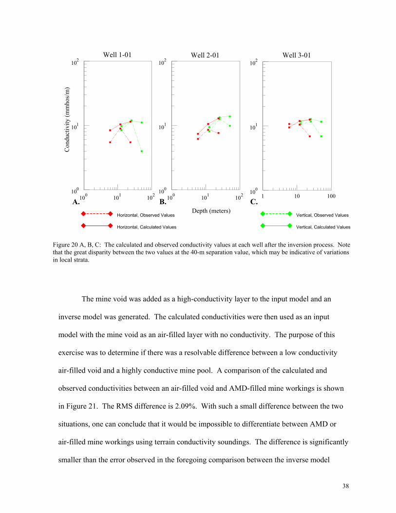
Figure 20 A, B, C: The calculated and observed conductivity values at each well after the inversion process. Notethat the great disparity between the two values at the 40-m separation value, which may be indicative of variationsin local strata.

The mine void was added as a high-conductivity layer to the input model and an

inverse model was generated. The calculated conductivities were then used as an input

model with the mine void as an air-filled layer with no conductivity. The purpose of this

exercise was to determine if there was a resolvable difference between a low conductivity

air-filled void and a highly conductive mine pool. A comparison of the calculated and

observed conductivities between an air-filled void and AMD-filled mine workings is shown

in Figure 21. The RMS difference is 2.09%. With such a small difference between the two

situations, one can conclude that it would be impossible to differentiate between AMD or

air-filled mine workings using terrain conductivity soundings. The difference is significantly

smaller than the error observed in the foregoing comparison between the inverse model

Depth (meters)

100 101 102

Con

duct

ivity

(mm

hos/

m)

100

101

102Well 1-01

100 101 102100

101

102Well 2-01

1 10 100100

101

102Well 3-01

Horizontal, Observed Values

Horizontal, Calculated Values

Vertical, Observed Values

Vertical, Calculated Values

A. B. C.

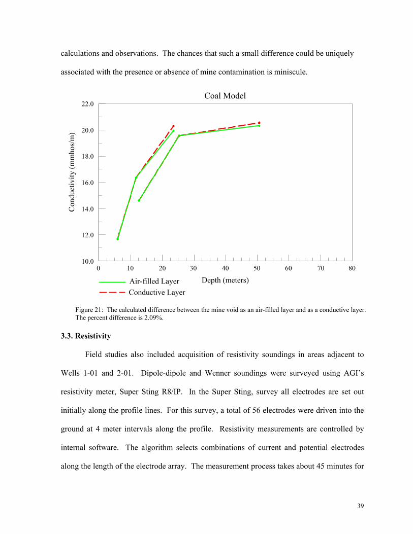
39

calculations and observations. The chances that such a small difference could be uniquely

associated with the presence or absence of mine contamination is miniscule.

Depth (meters)0 10 20 30 40 50 60 70 80

Con

duct

ivity

(mm

hos/

m)

10.0

12.0

14.0

16.0

18.0

20.0

22.0Coal Model

Air-filled Layer Conductive Layer

3.3. Resistivity

Field studies also included acquisition of resistivity soundings in areas adjacent to

Wells 1-01 and 2-01. Dipole-dipole and Wenner soundings were surveyed using AGI’s

resistivity meter, Super Sting R8/IP. In the Super Sting, survey all electrodes are set out

initially along the profile lines. For this survey, a total of 56 electrodes were driven into the

ground at 4 meter intervals along the profile. Resistivity measurements are controlled by

internal software. The algorithm selects combinations of current and potential electrodes

along the length of the electrode array. The measurement process takes about 45 minutes for

Figure 21: The calculated difference between the mine void as an air-filled layer and as a conductive layer.The percent difference is 2.09%.

40

the dipole-dipole survey and 2 hours for the Wenner survey. Data from the resistivity

soundings are then imported into Microsoft’s Excel to extract individual soundings. The

soundings were imported into RES2DINV (www.geoelectrical.com), a program which

generates a 2-D inverse resistivity model using a smoothness-constrained least-squared

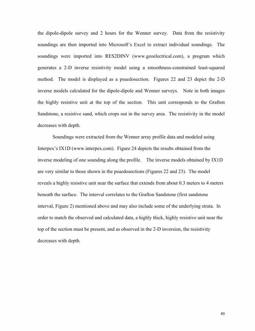
method. The model is displayed as a psuedosection. Figures 22 and 23 depict the 2-D

inverse models calculated for the dipole-dipole and Wenner surveys. Note in both images

the highly resistive unit at the top of the section. This unit corresponds to the Grafton

Sandstone, a resistive sand, which crops out in the survey area. The resistivity in the model

decreases with depth.

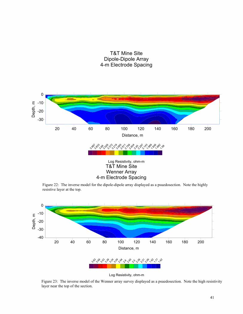
Soundings were extracted from the Wenner array profile data and modeled using

Interpex’s IX1D (www.interpex.com). Figure 24 depicts the results obtained from the

inverse modeling of one sounding along the profile. The inverse models obtained by IX1D

are very similar to those shown in the psuedosections (Figures 22 and 23). The model

reveals a highly resistive unit near the surface that extends from about 0.3 meters to 4 meters

beneath the surface. The interval correlates to the Grafton Sandstone (first sandstone

interval, Figure 2) mentioned above and may also include some of the underlying strata. In

order to match the observed and calculated data, a highly thick, highly resistive unit near the

top of the section must be present, and as observed in the 2-D inversion, the resistivity

decreases with depth.

41

1.58

1.682

1.836

1.989

2.143

2.297

2.45

2.604

2.758

2.911

3.065

3.219

3.372

3.526

3.68

3.833

3.987

20 40 60 80 100 120 140 160 180 200Distance, m

-30

-20

-10

0

Dep

th, m

T&T Mine SiteDipole-Dipole Array

4-m Electrode Spacing

Log Resistivity, ohm-m

1.62

1.77

1.92

2.06

2.21

2.36

2.52.65

2.82.94

3.09

3.24

3.38

3.53

3.68

3.83

20 40 60 80 100 120 140 160 180 200Distance, m

-40

-30

-20

-10

0

Dep

th, m

Log Resistivity, ohm-m

T&T Mine SiteWenner Array

4-m Electrode SpacingFigure 22: The inverse model for the dipole-dipole array displayed as a psuedosection. Note the highlyresistive layer at the top.

Figure 23: The inverse model of the Wenner array survey displayed as a psuedosection. Note the high resistivitylayer near the top of the section.

42

The results of resistivity modeling indicate that the highly resistive layer near the top

of the section serves as a barrier to current flow into the deeper section. A high resistivity

interval (low conductivity) also appears in each of the terrain conductivity models.

However, in the case of terrain conductivity surveys, the propagation of transmitted

electromagnetic waves is not impeded by the presence of a low conductivity interval.

Figure 24: The graph on the left is the observed and calculated resistivity data from the sounding performed inareas adjacent to Wells 1-01 and 2-01. Note the high data point has been masked and not included in thecalculations. The graph on the right is layered inversion of the resistivity data. The high resistivity intervalcorrelated with the Grafton Sandstone. The RMS difference between the calculated and observed resistivity data is16.77%.

1 10 100

100

1000

4

10

T and T M ine - W enner A r

Appa

rent R

esisti

vity

(ohm-

m)

Spacing (m )

JenniferM abie

0.1 1 10 100 1000

4

10

0 .1

1

10

1 00

1 000

Depth

(m)

R esistiv ity (ohm -m )

43

Problems in resistivity surveys can arise when highly resistive units are present in the

subsurface. The resistivity response at target depths cannot be measured in when overlying

highly resistive zones inhibit current flow to the target interval (Merkel, 1972). The high

resistive near surface layer observed in this study prevents measurements of meaningful

apparent resistivity from depths below approximately 10 meters. Layers in the models

appearing below a depth of a few meters appear to have a lower resistivity and are most

likely due to limited current flow through deeper intervals.

3.4. Time Domain Electromagnetic Methods

Two time domain electromagnetic (TDEM) surveys were completed in areas adjacent

to Wells 1-01, 2-01, and 3-01. Due to improper instrument configuration and possible

instrument failure, no useful data was collected. Another survey with proper instrument

configuration would be useful as TDEM soundings are able to resolve conductors at depths

greater than those obtained with terrain conductivity soundings. Other methods, such as

controlled-source audio frequency magneto-telluric (CSAMT), which have been used for

groundwater exploration and monitoring, are being investigated by the US Department of

Energy in order to determine if such technology is applicable in an environmental

application.

44

Chapter 4 - Airborne Analysis Results and Discussion

4.1. Airborne Electromagnetic Conductivity

Five frequencies of airborne electromagnetic data were collected over the T&T Mine

Complex as part of the Muddy Creek/Roaring Creek Watershed airborne survey. The data

were collected using Fugro’s DIGHEMVRES electromagnetic data acquisition system. The

frequencies ranged from 390 Hz to 102,680 Hz. The flight lines over the T&T mine site

were extracted and imported into EM Flow, an airborne electromagnetic (EM) modeling

program (Macnae, 2001).

EM Flow, developed by CRCAMET, an Australian minerals exploration research

organization, uses theoretically defined EM system waveforms to deconvolve measured EM

multi-component, multi-channel line data. The software is designed to operate on large EM

datasets such as the T&T data set and provide conductivity-depth images (CDI), plus

anomaly identification and modeling tools (Macnae, 2001).

Conversion of observed EM data to time constant (Tau) domain is achieved by

deconvolving the input data with a pre-computed ideal waveform (Macnae, 2001). A typical

modeling operation involves analysis of one or a select group of traverse lines and their

acquired EM data. The appropriate Tau analysis range is defined, the controlling parameters

are selected, and then the deconvolution and the CDI creation process can be applied to the

selected dataset and allowed to operate in a batch style of operation (Macnae, 2001).

Topography is taken into account for depth solutions and will form the upper surface of the

CDI’s. All flight lines for the T&T Mine Complex were processed, but for the purpose of

this study, only the flight lines that corresponded with well location are considered.

45

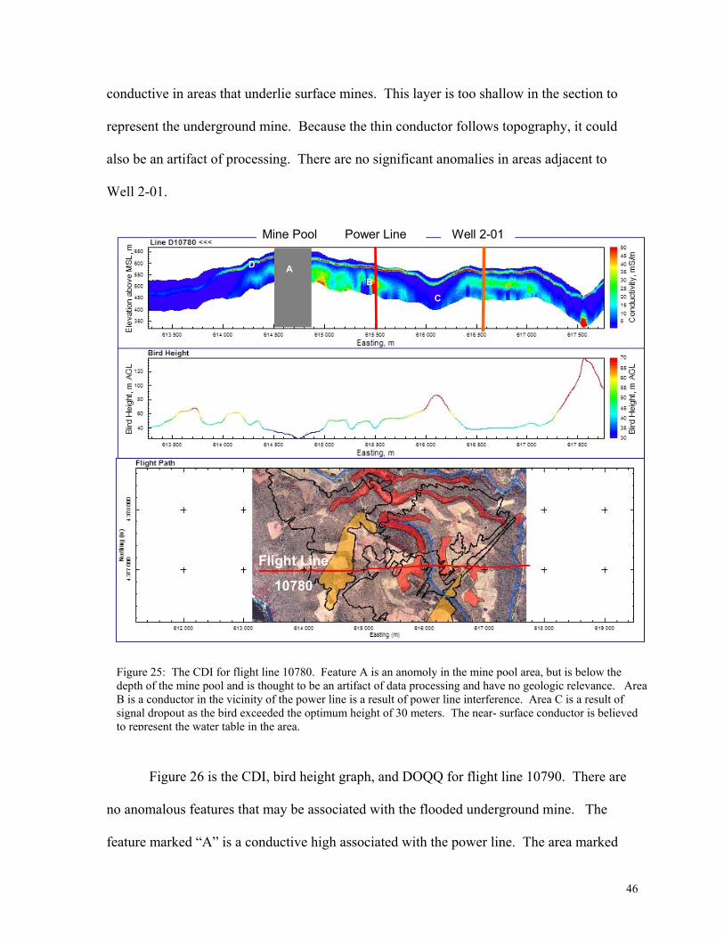
Figures 25, 26, and 27 are conductivity-depth images (CDI) for flight lines 10780,

1790, and 10850, which are in close proximity to wells 1-01, 2-01, and 3-01 from the T&T

Mine Complex. A digital orthophoto quarter quadrangle (DOQQ) is coupled with each CDI

in order to indicate the flight line location, shown by a heavy red line, in relation to the wells.

Portions of these flight lines overlie approximately 90-m deep, partially flooded, mine

workings indicated in orange on Figures 25-27. The water in the flooded mine is known to

be conductive (>500 mS/m). The elevation (in meters) is indicated on the side of the CDI

and represents topography. Information included on each CDI are the corresponding flooded

mine areas (orange shading), the power line locations (vertical red lines), and well locations

(vertical orange lines).

Figure 25 is the CDI and DOQQ for flight line 10780. The feature marked “A”

represents an unknown anomaly of high conductivity. The depth of this conductive area is

about 160 meters below the surface – too deep in the section to be considered for the flooded

mine. The feature marked “B” is an anomaly associated with the power line. The deep

anomaly in the vicinity of the power line is the result of interference. The area marked “C”

is a topographic low. In this area, the bird height greatly exceeded the optimum bird height

of 30 meters, resulting in a signal dropout. No useful data can be obtained from this low

area. Additionally, the flying height of the bird exceeded 30 meters at the end of each flight

line, making data obtained at flight line ends of no value. There are several deep, conductive

features that were identified below the exploration depth for the frequencies used and also

below the depth of the mine pool. These conductors are believed to be artifacts of data

processing and have no geological relevance. The feature marked “D” is a near-surface

conductor (appears as a thin, yellow band) that could represent the water table; it is more

46

conductive in areas that underlie surface mines. This layer is too shallow in the section to

represent the underground mine. Because the thin conductor follows topography, it could

also be an artifact of processing. There are no significant anomalies in areas adjacent to

Well 2-01.

Figure 26 is the CDI, bird height graph, and DOQQ for flight line 10790. There are

no anomalous features that may be associated with the flooded underground mine. The

feature marked “A” is a conductive high associated with the power line. The area marked

Figure 25: The CDI for flight line 10780. Feature A is an anomoly in the mine pool area, but is below thedepth of the mine pool and is thought to be an artifact of data processing and have no geologic relevance. AreaB is a conductor in the vicinity of the power line is a result of power line interference. Area C is a result ofsignal dropout as the bird exceeded the optimum height of 30 meters. The near- surface conductor is believedto represent the water table in the area.

Flight Line

10780

Mine Pool Power Line Well 2-01

CB

AD

Flight Line

10780

Mine Pool Power Line Well 2-01

Flight Line

10780

Mine Pool Power Line Well 2-01

CB

AD

47

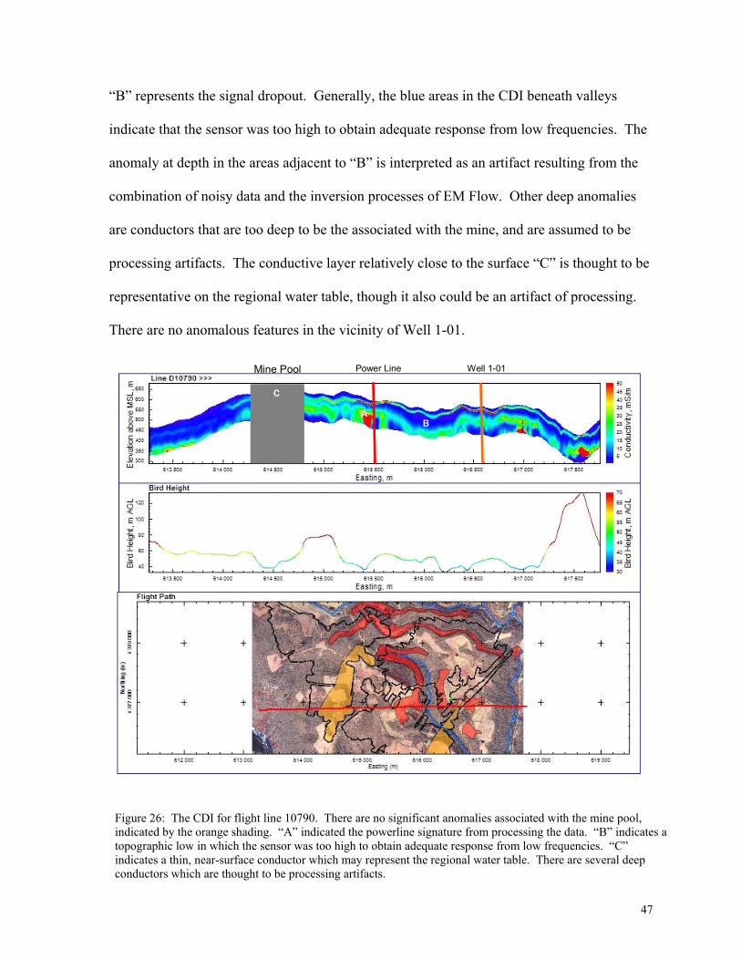
“B” represents the signal dropout. Generally, the blue areas in the CDI beneath valleys

indicate that the sensor was too high to obtain adequate response from low frequencies. The

anomaly at depth in the areas adjacent to “B” is interpreted as an artifact resulting from the

combination of noisy data and the inversion processes of EM Flow. Other deep anomalies

are conductors that are too deep to be the associated with the mine, and are assumed to be

processing artifacts. The conductive layer relatively close to the surface “C” is thought to be

representative on the regional water table, though it also could be an artifact of processing.

There are no anomalous features in the vicinity of Well 1-01.

AB

Power Line Well 1-01Mine Pool

C

AB

Power Line Well 1-01Mine Pool

C

Figure 26: The CDI for flight line 10790. There are no significant anomalies associated with the mine pool,indicated by the orange shading. “A” indicated the powerline signature from processing the data. “B” indicates atopographic low in which the sensor was too high to obtain adequate response from low frequencies. “C”indicates a thin, near-surface conductor which may represent the regional water table. There are several deepconductors which are thought to be processing artifacts.

48

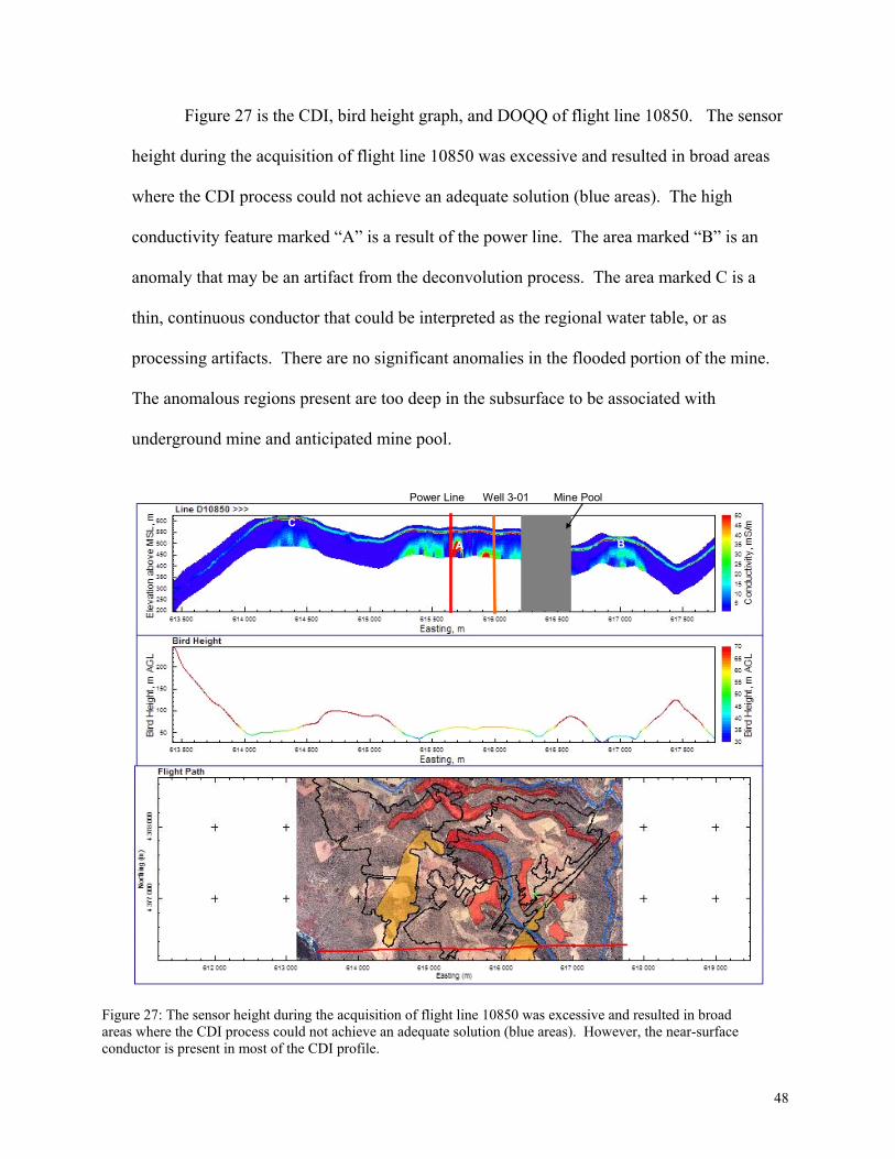
Figure 27 is the CDI, bird height graph, and DOQQ of flight line 10850. The sensor

height during the acquisition of flight line 10850 was excessive and resulted in broad areas

where the CDI process could not achieve an adequate solution (blue areas). The high

conductivity feature marked “A” is a result of the power line. The area marked “B” is an

anomaly that may be an artifact from the deconvolution process. The area marked C is a

thin, continuous conductor that could be interpreted as the regional water table, or as

processing artifacts. There are no significant anomalies in the flooded portion of the mine.

The anomalous regions present are too deep in the subsurface to be associated with

underground mine and anticipated mine pool.

Figure 27: The sensor height during the acquisition of flight line 10850 was excessive and resulted in broadareas where the CDI process could not achieve an adequate solution (blue areas). However, the near-surfaceconductor is present in most of the CDI profile.

Well 3-01Power Line

A B

C

Mine PoolWell 3-01Power Line

A B

C

Mine Pool

49

No CDI indicated a conductive anomaly at the depth and location of the mine pool.

The average depth to the mine pool is about 90 m along the flight lines, which is near the

calculated exploration depth for the 390-Hz frequency. However, the 390 Hz data could not

be used in the construction of CDI profiles because of excessive noise. Some of the noise

can be attributed to the high-voltage power line that extends across the site perpendicular to

flight lines, and was therefore unavoidable. Additional noise occurred as a result of excessive

sensor height and the swinging of the bird, which can be attributed to an inexperienced pilot.

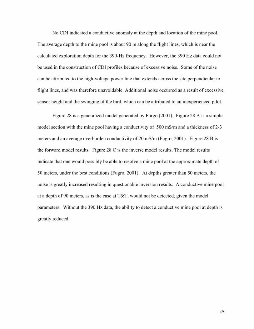
Figure 28 is a generalized model generated by Furgo (2001). Figure 28 A is a simple

model section with the mine pool having a conductivity of 500 mS/m and a thickness of 2-3

meters and an average overburden conductivity of 20 mS/m (Fugro, 2001). Figure 28 B is

the forward model results. Figure 28 C is the inverse model results. The model results

indicate that one would possibly be able to resolve a mine pool at the approximate depth of

50 meters, under the best conditions (Fugro, 2001). At depths greater than 50 meters, the

noise is greatly increased resulting in questionable inversion results. A conductive mine pool

at a depth of 90 meters, as is the case at T&T, would not be detected, given the model

parameters. Without the 390 Hz data, the ability to detect a conductive mine pool at depth is

greatly reduced.

50

Figure 28 A, B, C, D: Forward model constructed using a 2-m thick mine pool by Fugro (2001). Figure A is the model frequency data. All five frequencies were used and noise was introduced into the data. Figure B is a simple model section with the mine pool having a conductivity of 500 mS/m and an average overburden conductivity of 20 mS/m (Fugro, 2001). Figure C is the forward model results. Figure D is the inverse model results.

B.

C.

D.

A.

B.

C.

Figure 28 A, B, C: Forward model constructed using a 2-m thick mine pool by Fugro (2001). FigureA is a simple model section with the mine pool having a conductivity of 500 mS/m and an averageoverburden conductivity of 20 mS/m (Fugro, 2001). Figure B is the forward model result. Figure Cis the inverse model result.

51

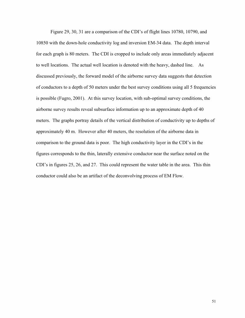
Figure 29, 30, 31 are a comparison of the CDI’s of flight lines 10780, 10790, and

10850 with the down-hole conductivity log and inversion EM-34 data. The depth interval

for each graph is 80 meters. The CDI is cropped to include only areas immediately adjacent

to well locations. The actual well location is denoted with the heavy, dashed line. As

discussed previously, the forward model of the airborne survey data suggests that detection

of conductors to a depth of 50 meters under the best survey conditions using all 5 frequencies

is possible (Fugro, 2001). At this survey location, with sub-optimal survey conditions, the

airborne survey results reveal subsurface information up to an approximate depth of 40

meters. The graphs portray details of the vertical distribution of conductivity up to depths of

approximately 40 m. However after 40 meters, the resolution of the airborne data in

comparison to the ground data is poor. The high conductivity layer in the CDI’s in the

figures corresponds to the thin, laterally extensive conductor near the surface noted on the

CDI’s in figures 25, 26, and 27. This could represent the water table in the area. This thin

conductor could also be an artifact of the deconvolving process of EM Flow.

52

Descriptor - include initials, /org#/date

Well 1-01

CDI Induction Log Inversion ModelD

epth (meters)

0

10

20

30

40

50

60

70

80

Conductivity (mmhos/m)0 10 20 30 40 50 60 70

Well 1-01

Depth (m

eters)

0

10

20

30

40

50

60

70

80

Conductivity (mmhos/m)0 10 20 30 40 50 60 70

Well 1-01

Figure 29 A, B, C: A comparison of the airborne, borehole induction log, and the inverse model for Well1-01. The well location is denoted with a black dashed line on Figure A. The elevation is located on theleft of figure A, the conductivity (mS/m) is denoted with the color bar on the right of Figure A. Figure Bis the conductivity log. Figure C is the starting model (green line) and the inverse model (red, dashedline) for the EM-34 soundings at Well 1.

53

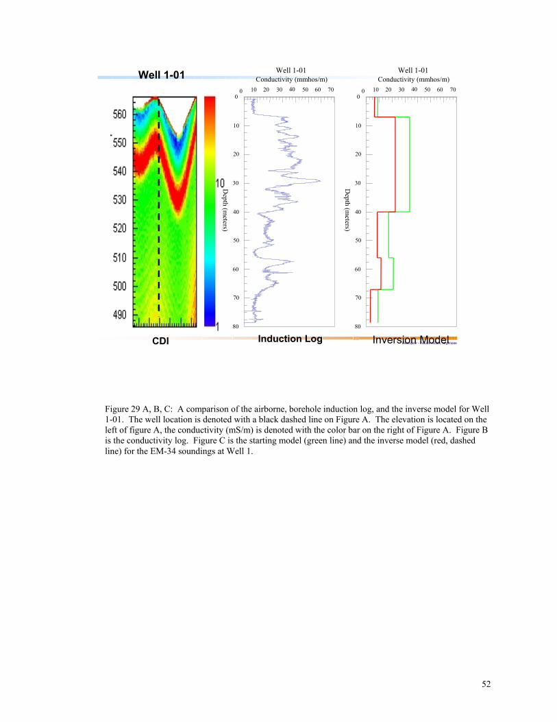
Figure 30 A, B, C: A comparison of the airborne, borehole induction log, and the inverse model for Well2-01. The well location is denoted with a black dashed line on Figure A. The elevation is located on theleft of figure A, the conductivity (mS/m) is denoted with the color bar on the right of Figure A. Figure Bis the conductivity log. Figure C is the starting model (green line) and the inverse model (red, dashedline) for the EM-34 soundings at Well 2.

Descriptor - include initials, /org#/date

Induction Log CDI Inversion Model

Well 2-01

Depth (m

eters)

0

10

20

30

40

50

60

70

80

Conductivity (mmhos/m)0 10 20 30 40 50 60 70

Well 2-01

Depth (m

eters)

0

10

20

30

40

50

60

70

80

Conductivity (mmhos/m)0 10 20 30 40 50 60 70

Well 2-01

54

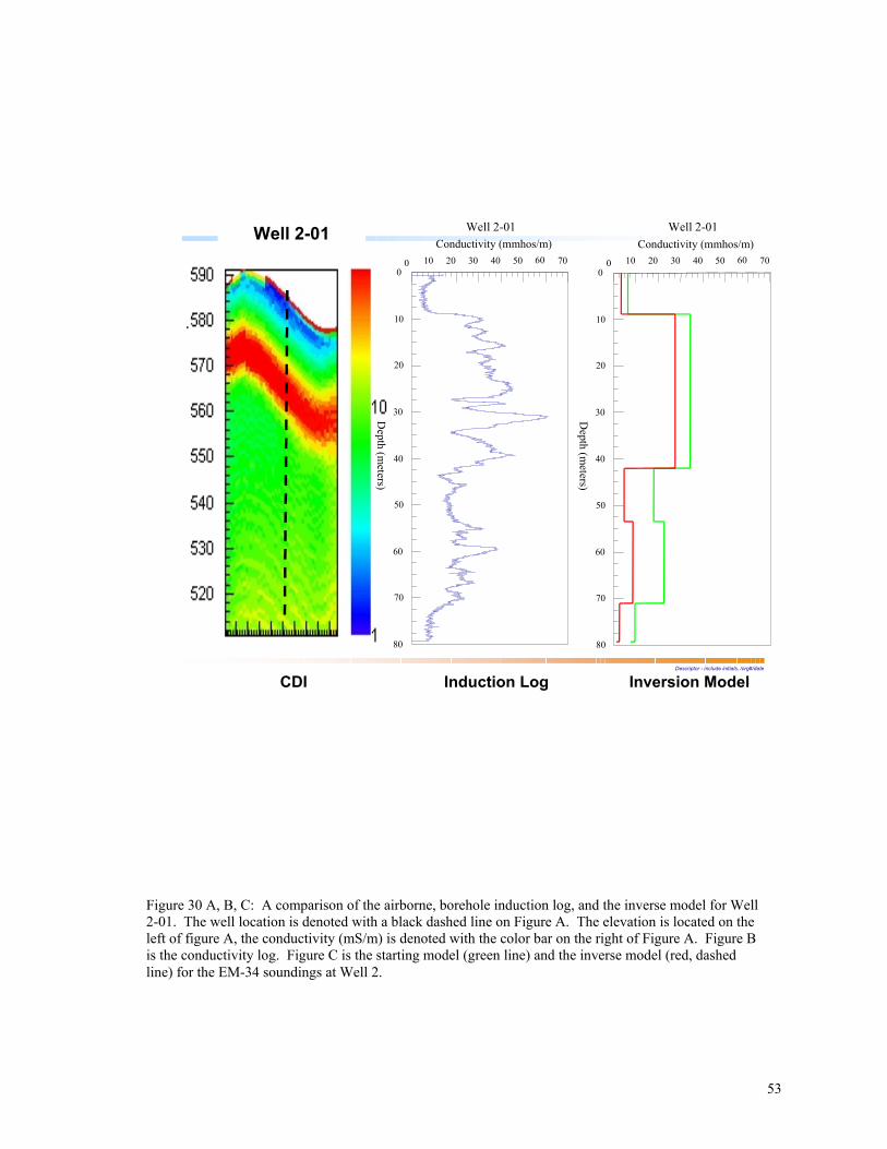
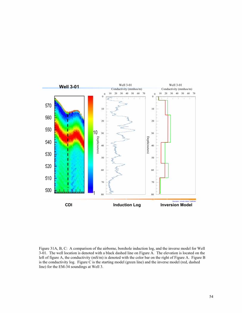
Figure 31A, B, C: A comparison of the airborne, borehole induction log, and the inverse model for Well3-01. The well location is denoted with a black dashed line on Figure A. The elevation is located on theleft of figure A, the conductivity (mS/m) is denoted with the color bar on the right of Figure A. Figure Bis the conductivity log. Figure C is the starting model (green line) and the inverse model (red, dashedline) for the EM-34 soundings at Well 3.

Descriptor - include initials, /org#/date

Well 3-01

CDI Induction Log Inversion Model

Depth(m

eters)

0

10

20

30

40

50

60

70

80

Conductivity (mmhos/m)0 10 20 30 40 50 60 70

Well 3-01

Depth(m

eters)0

10

20

30

40

50

60

70

80

Conductivity (mmhos/m)0 10 20 30 40 50 60 70

Well 3-01

55

4.2. Thermal Infrared Imagery

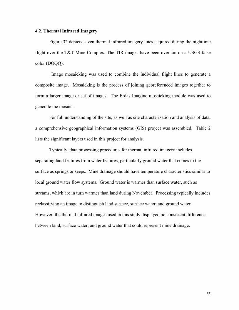
Figure 32 depicts seven thermal infrared imagery lines acquired during the nighttime

flight over the T&T Mine Complex. The TIR images have been overlain on a USGS false

color (DOQQ).

Image mosaicking was used to combine the individual flight lines to generate a

composite image. Mosaicking is the process of joining georeferenced images together to

form a larger image or set of images. The Erdas Imagine mosaicking module was used to

generate the mosaic.

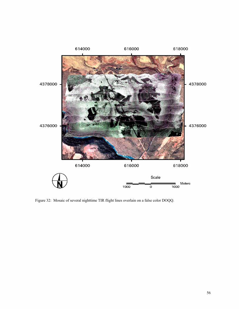
For full understanding of the site, as well as site characterization and analysis of data,

a comprehensive geographical information systems (GIS) project was assembled. Table 2

lists the significant layers used in this project for analysis.

Typically, data processing procedures for thermal infrared imagery includes

separating land features from water features, particularly ground water that comes to the

surface as springs or seeps. Mine drainage should have temperature characteristics similar to

local ground water flow systems. Ground water is warmer than surface water, such as

streams, which are in turn warmer than land during November. Processing typically includes

reclassifying an image to distinguish land surface, surface water, and ground water.

However, the thermal infrared images used in this study displayed no consistent difference

between land, surface water, and ground water that could represent mine drainage.

56

Figure 32: Mosaic of several nighttime TIR flight lines overlain on a false color DOQQ.

57

Theme Type DescriptionTIR_image (lines

3-10) raster Thermal Infrared Image by LineStudy_Area_DEM raster Study Area, USGS Digital Elevation ModelStudy_Area_DRG raster Study Area, USGS Digital Raster GraphicStudy_Area_DOQ raster Study Area, USGS Digital Ortho Quarter Quad

Upper FreeportStruct raster

Study Area, Structure contours of UpperFreeport Coal

Con_102K raster Apparent Conductivity Map, 102680 HzCon_25K raster Apparent Conductivity Map, 25800 HzCon_6200 raster Apparent Conductivity Map, 6254 HzCon_1500 raster Apparent Conductivity Map,1555 HzCon_380 raster Apparent Conductivity Map, 380 Hz

Mine Boundary polygon Extent of Underground MineMine_Pools polygon Extent of Mine Pools

Surface_Mined polygon Extent of Surface Mined AreasPreston County polygon Boundary of Preston County

Preston Anticine line Preston AnticlineKingwood Syncline line Kingwood Syncline

Mine_streams line Streams near mining areaWell_location point Well locations in mine area

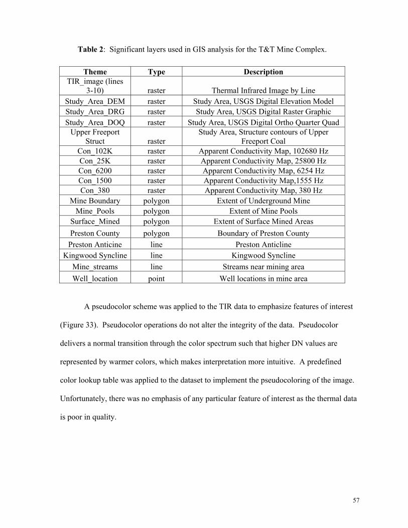
A pseudocolor scheme was applied to the TIR data to emphasize features of interest

(Figure 33). Pseudocolor operations do not alter the integrity of the data. Pseudocolor

delivers a normal transition through the color spectrum such that higher DN values are

represented by warmer colors, which makes interpretation more intuitive. A predefined

color lookup table was applied to the dataset to implement the pseudocoloring of the image.

Unfortunately, there was no emphasis of any particular feature of interest as the thermal data

is poor in quality.

Table 2: Significant layers used in GIS analysis for the T&T Mine Complex.

58

Erdas Imagine has a swipe tool, which allows the user to view two overlain images in

a single viewer at the same time. Using this tool, thermal anomalies were located and

interpreted. Figure 34 depicts a cluster of thermal anomalies that appear to be livestock.

Figure 33: A pseudocolor image of the thermal data. Pseudocoloring was applied in order to highlightpossible areas of interest. The applied color scheme is intuitive in nature; red colors are the warmest, bluecolors are coolest.

59

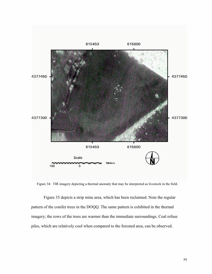
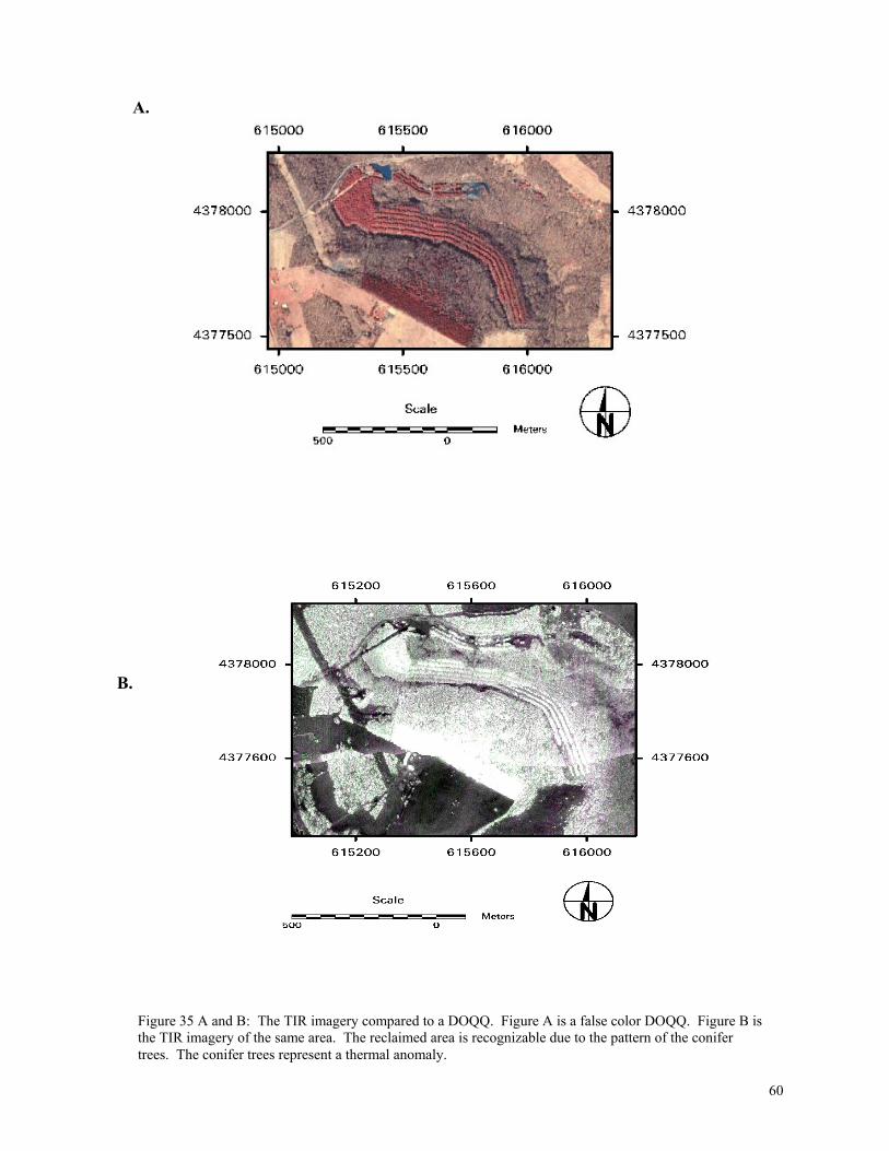
Figure 35 depicts a strip mine area, which has been reclaimed. Note the regular

pattern of the conifer trees in the DOQQ. The same pattern is exhibited in the thermal

imagery; the rows of the trees are warmer than the immediate surroundings. Coal refuse

piles, which are relatively cool when compared to the forested area, can be observed.

Figure 34: TIR imagery depicting a thermal anomaly that may be interpreted as livestock in the field.

60

Figure 35 A and B: The TIR imagery compared to a DOQQ. Figure A is a false color DOQQ. Figure B isthe TIR imagery of the same area. The reclaimed area is recognizable due to the pattern of the conifertrees. The conifer trees represent a thermal anomaly.

B.

A.

61

Although TIR has been found to be successful in locating AMD in previous studies (Sams

and Velsoski, 2003), several environmental conditions can limit the effectiveness of using

thermal infrared as a method for locating potential mine drainage source areas. First, the

path between the source and the airborne sensor must be unobstructed. In forested areas, a

leaf-off period is usually selected for data collection. Under normal circumstances in the

deciduous temperate forested areas of the same latitude (39°N) and elevation range (950-

2000 feet) of this study, this period ranges from late October to early April. However, the

T&T Mine Complex survey was performed at the beginning of a leaf-off period (November),

and it is possible that some trees had not yet lost all of their leaves. In addition, even areas

heavily forested with deciduous trees may be obstructed by tree trunks and branches.

Furthermore, evergreen species were a problem for this study, particulary those species

planted in the reclamation of the T&T mine site. In most instances, the coniferous trees

obscured thermal emissions from the ground, precluding the possibility of locating features

that would otherwise be expected to exhibit strong thermal responses such as a possible mine

drainage seep. Additionally, the leaves of coniferous trees exhibit a relatively high radiant

temperature due to the thermal storage and emissive properties of the leaves. These warm

temperatures associated with conifer trees can be confused with the warm temperatures of

the mine drainage.

62

Chapter 5 – Conclusions and Significance

5.1. Key Findings

Ground Surveys

Terrain conductivity and resistivity soundings were acquired at the T&T mine

complex to determine whether they might prove useful for detecting and mapping

underground mine pools. The inverse modeling of the terrain conductivity soundings

indicates that the mine pool could not be resolved at it’s depth of 90 meters. The differences

between the observed conductivities and the calculated conductivities could be attributed to

local variations in the strata. Another explanation for the differences between the observed

and calculated conductivities could be a result of dewatering of upper aquifers via fractures

propagating upward from the mine. As the overlying strata subside into the mine void,

extension fractures develop. These fractures extend upward into the shallower strata and

may penetrate aquifers, allowing for dewatering of the aquifer into lower strata.

Forward conductivity models show that at the depth of 90 meters, the anomaly

produced by the mine interval is too small to be detected. Useful information was obtained

from the terrain conductivity surveys on the properties of strata in the upper 40 meters.

The resistivity surveys were also unable to resolve resistivity variations associated

with the mine workings. Observation of layer resistivities at depths below approximately 10

meters was obscured by the presence of the near-surface highly resistive Grafton Sandstone.

This high resistivity layer inhibits electric current flow into deeper formations, making the

resistivity survey ineffective. Resistivity models derived from the individual resistivity

sounding yielded results similar to those obtained from 2-D inversion of the entire profile.

63

Airborne Surveys

An airborne electromagnetic and thermal infrared imaging survey was conducted

over the T&T Mine Complex to detect potential pollution sources in the Roaring

Creek/Muddy Creek watershed area. Another objective of the airborne EM survey was to

determine whether these airborne surveys could be used to characterize the near-surface

hydrology in coal mining areas. The ability to detect abandoned flooded mine workings in

the vicinity of active mines would help avoid accidental breakthrough into the old mine

systems.

The airborne conductivity data was deconvolved using EM Flow (Macnae, 2001).

CDI’s were generated for all the flight lines over the T&T mining area, but for the purpose

of the study, only flight lines that corresponded to well locations were presented. When

computing models for the airborne data, the 390 Hz data had to be excluded due to excessive

power line noise. The comparison of airborne CDI’s with down-hole induction logs and EM

34 soundings show some agreement. The thin, near-surface conductor could be a result of

the deconvolving process. However, the airborne data results do not corroborate ground

survey results.

As projected by the forward model of the airborne conductivity data, a conductive

mine pool may be detected under optimal conditions at depth of approximately 40 meters.

Therefore, there was little chance that the survey at the T&T Mine Complex could detect

conductive mine pools at 90-m depth. Furthermore, the execution of this survey was sub-

optimal. Should the airborne survey be conducted such that the bird maintained the optimal

height above ground (30m) and the study area had minimal powerline and cultural

64

interference, the HEM survey results may have detected mine pools up to a depth of

approximately 40 meters.

The CDI’s do not indicate a conductive anomaly at the depth and location of the

known conductive mine pool. There is a conductive layer near the surface that roughly

follows topography. This conductive layer is thought to correspond with the highly

conductive layer observed in the well logs, and could be the local water table. The

conductive anomalous regions observed at depth are much deeper than the mine pools and

are thought to be a result of noise. Distinctive anomalous regions at depth are associated

with power line location and areas in which the maximum sensor height was greatly

exceeded.

The average depth to the mine pool is about 90 m along the flight lines, which is

much greater than the depth limit for detection under optimal conditions. However,

correctable problems with this survey may have been responsible for the non-detection of the

mine pool. The 390 Hz data could not be used in forward modeling calculations due to noisy

data because the external noise precluded the depth advantage. Some noise can be attributed

to the high-voltage power line that extends across the site and is unavoidable. Rugged

topography, an inexperienced helicopter pilot, excessive sensor height, swinging of the bird,

and interference from power lines resulted in sub-optimal survey execution and noisy data.

The mine pools were not detected.

Thermal imagery has been successfully used to detect groundwater discharging at the

surface in mining areas in the Appalachian region in order to further characterize

watersheds. However, the thermal infrared imagery collected at the T&T Mine Complex

was not useful in determining potential acid mine drainage discharge points. The survey

65

was undertaken during the leaf-off period, however, the numerous coniferous trees obscured

the ground thermal patterns. Anomalies present in the TIR images of the T and T Mine

Complex are not associated with groundwater discharge, but rather cultural features and

forested areas, including both natural forestlands and reclaimed areas.

5.2. Significance of Findings

This study provided an opportunity to evaluate the use of airborne and ground

geophysical and remote sensing techniques to detect mine pools and possible acid mine

drainage source areas in an area with both underground and surface mine sites. This study

served as a benchmark for the potential of geophysical methods for mine site evaluation.

Though the surveys did not successfully delineate the mined areas, they should serve as a

starting point for further investigations for the use of geophysical methods in an

environmental application. Previous studies have shown that airborne and ground-based

geophysics and remote sensing can be successfully employed to delineate vertical and

horizontal extents of mined areas. This study shows the potential and limitations of

geophysical survey methods conducted to resolve near surface conductivity and resistivity

variations over underground mine complexes.

5.3. Suggestions for Future Work

Future geophysical efforts at such sites should utilize modeling efforts before

geophysical surveys are planned in order to determine if areas of interest can be detected

using this methodology.

For airborne geophysical surveys, planners should if possible avoid areas with

significant sources of cultural interferences such as power lines, towns, and pipelines. A

pilot who is comfortable and experienced flying a sling load in rugged terrain should be

66

employed for such survey endeavors. When considering a nighttime thermal infrared survey,

planners should ensure that the flight takes place in a leaf-off period and in an area that is not

dominated with coniferous trees.

Ground surveys should be strategically located to minimize depth to the target

intervals. Mine pool depth at the T&T Mine Complex exceeded 80 meters at ground survey

locations, a depth too great to be accurately sensed using the geophysical methods employed

in this study.

67

References

Ackman, T.E., G.A. Veloski, R.A. Dotson, Jr., R.W. Hammack. An Evaluation of

Remote Sensing Technologies for Watershed Assessment. U.S.

Department of Energy, National Energy Technology Laboratory,

Pittsburgh, PA.

Ackman, T.E., and K.K. Cohen, 1994. Geophysical Methods: Remote

Techniques Applied to Mining-related Environmental and

Engineering Problems. U.S. Department of Energy, National Energy

Technology Laboratory, Pittsburgh, PA.

Burger, Robert H. 1992. Exploration Geophysics of the Shallow Subsurface.

pp. 310,405.

Brewster, S. B. 1999. Geometric Correction System Capabilities, Processing, and

Applications, Fourth International Airborne Remote Sensing Conference and

Exhibition/21st Canadian Symposium

Fugro-Geoterrex Dighem, Inc., 2000. Report for US Dept. of Energy, Federal

Energy and Technology Center over the Cheat River Watershed,

#996004.

Hammack, R. W., and Mabie, J.S., 2002. The Use of Airborne EM Conductivity to Locate

Contaminant Flow Paths at the Sulphur Bank Mercury Mine Superfund

Site. Proceedings for the Symposium on the Application of Geophysics to

Environmental and Engineering Problems, Feb 10-14.

Keller, George V., 1997. Principles of Time-Domain Electromagnetic (TDEM)

Sounding. The Leading Edge, April: 355-357.

Keller, George V. and Frischknecht, Frank C., 1966. Electrical Methods in Geophysical

Prospecting. Oxford, New York, Pergamon Press.

Keys, S.W., 1988. Borehole Geophysics Applied to Groundwater Investigations.

Techniques of Water Resource Investigations of U.S. Geological Survey,

Book 2, Chapter E2: 1-105.

King, A.R. and Hynes, T., 1994. Application of Geophysical Methods for

Monitoring Acid Mine Drainage. Proceedings for International Land

Reclamation and Mine Drainage Conference, April 24-29: 317-326.

68

Interpex Limited, 2001. www.interpex.com/em.htm

Ladwig, Kenneth, 1983. Electromagnetic Induction Methods for Monitoring

Acid Mine Drainage. Ground Water Monitoring Review. Winter: 46-51.

Lillesand, T. M. and Kiefer, R. W. (1994), Remote Sensing and Image Interpretation, New York: John Wiley & Sons, Inc. 3rd Ed.

McNeill, J.D. 1980-a. Electrical Conductivity of Soils and Rocks. Geonics

Limited, TN-5.

McNeill, J.D. 1980-b. Electromagnetic Terrain Conductivity Measurements at Low

Induction Numbers. Geonics Limited, TN-6.

McNeill, J.D., 1980-c. Application of Transient Electromagnetic Techniques.

Geonics Limited, TN-7.

McNeill, J.D. and V.F. Labson. Geologic Mapping using VLF Radio Fields

pp.521-640.

McNeill, J.D., 1990. Use of Electromagnetic Methods for Groundwater

Exploration in Geotechnical and Environmental Geophysics.

Investigations in Geophysics, S.H. Ward (ed.), no. 5: 191-218.

Mabie, J.S., Hammack, R.W., and Veloski, G.A., 2002. Airborne and

Ground-Based Investigations of the North Fork of Yellow Creek, Jefferson County,

Ohio. Proceedings for the Acid Mine Drainage Task Force, April.

Macnae, James, 2001. EM Flow Experienced User Manual, Version 5.10

http://www.encom.com.au/pages/swef.htm

Merkel, R.H., 1972. The Use of Resistivity Techniques to Delineat Acid Mine

Drainage in Ground Water. Ground Water, 10 (5): 38-42.

Tasci, M.T. and Jordan, J.M. Case Histories Using the Time Domain

Electromagnetic Sounding Method in Oil and Gas Exploration.

Submitted to Geophysics, Journal of Society of Exploration

Geophysicists.

www.geotech.org/survey/stratas/casehist/casehist.htm

Torgerson, C., Faux, R.N., McIntosh, B.A., Poage, N.J., Norton, D.J., 2001.

Airborne Thermal Remote Sensing for Water Temperature Assesement

in Rivers and Streams. Remote Sensing of the Environment, 76:386-398.

Sams, J. and Veloski, G, 2003, USDOE Report. Anaylsis of TIR data acquired for Kettle

69

Creek Watershed. Unpublished.

Stoller, R.L., and Roux, P., 1975. Earth Resistivity Surveys – A Method for

Defining Ground Water Contamination. Ground Water, 13(2): 145-150.

Stoyer, C.H., 1998. Vertical Resolution and Equivalence in EM Soundings. Interpex

Limited, SAGEEP Workshop.

Yazicigil, H. and Sendlein, V.A., 1982. Surface Geophysical Techniques in

Groundwater Monitoring Part II. Ground Water Monitoring Review, Winter.