NRL Report 7725

Geophysical Aspects of Atmospheric Refraction

CHARLES G. PURVES

Aerospace Systems BranchSpace Systems Division

June 7, 1974

NAVAL RESEARCH LABORATORYWashington, D.C.

Approved for public release; distribution unlimited.

SECURITY CLASSIFICATION OF THIS PAGE (When Data Entered)

READ INSTRUCTIONSREPORT DOCUMENTATION PAGE BEFORE COMPLETING FORM

I. REPORT NUMBER 2, GOVT ACCESSION NO. 3. RECIPIENT'S CATALOG NUMBER

NRL Report 77254. TITLE (and Subtitle) S. TYPE OF REPORT & PERIOD COVERED

Final report on one phase of aGEOPHYSICAL ASPECTS OF ATMOSPHERIC continuing NRL Problem.REFRACTION 6. PERFORMING ORG. REPORT NUMBER

7, AUTHOR(s) S. CONTRACT OR GRANT NUMBER(s)

Charles G. Purves

9. PERFORMING ORGANIZATION NAME AND ADDRESS 10. PROGRAM ELEMENT, PROJECT, TASKAREA & WORK UNIT NUMBERS

Naval Research Laboratory NRL Problem R07-20Washington, D.C. 20375 RE 12-151-402-4024

II. CONTROLLING OFFICE NAME AND ADDRESS 12. REPORT DATEDepartment of the Navy June 7, 1974Office of Naval Research 13. NUMBER OF PAGES

Arlington, Va. 22217 4414. MONITORING AGENCY NAME & ADDRESS(If different from Controlling Office) IS. SECURITY CLASS. (of this report)

Unclassified

ISa. DECLASSIFICATION/DOWNGRADINGSCHEDULE

16. DISTRIBUTION STATEMENT (of this Report)

Approved for public release; distribution unlimited.

17. DISTRIBUTION STATEMENT (of the abstract enteredin Block 20, if different from Report)

18. SUPPLEMENTARY NOTES

19. KEY WORDS (Continue on reverse side if necessary and identify by block number)Anomalous radar propagation Electromagnetic waves Ray tracingCloud correlations Haze layers Refractive index forecastsCloud mosaic Microwave refractometer Refractive index profilesConvective cloud cells Radar horizon Satellite cloud photographyDucting gradients Radios (Continued)

20. ABSTRACT (Continue on reverse aide if necessary and identify by block number)

Considerable interest is being generated by the Navy on ways of improving the stateof the art in providing better refractive index forecasts (RIF's) needed to upgrade theNavy's capabilities in radar target detection, communication, and other significant propa-gation effects where atmospheric refraction poses a real concern during naval operations.For a decade during the late 1950's and early 1960's, personnel of the Naval ResearchLaboratory (NRL) conducted many radar meteorological research flights throughout theworld and especially in trade wind regions where anomalous propagation conditions are

(Continued)

DD 'JAN 73 1473 EDITION OF I NOV 65 IS OBSOLETE

S/N 0102-014- 6601 I ISECURITY CLASSIFICATION OF THIS PAGE (When Data ffntared)

C=

C-`�r-�;1111

-7

r1r

..LLIJRITY CLASSIFICATION OF THIS PAGE(Wh.n Data Entered)

19. Keywords (continued)

Temperature inversionTiros 3Experiments I-IV

20. Abstract (continued)

typically associated with a persistent temperature inversion. The intent of this reportis to compile many of the significant findings obtained by the NRL research flights sothat the geophysical aspects of atmospheric refraction can be viewed from both thetheoretical and practical points of view.

From a theoretical point of view a review of the literature is included to provide ageneral background covering such aspects as the wavelength dependence of atmosphericducts, the accepted equation for refractive index of air in terms of meteorological param-eters, refraction and reflection at a surface of discontinuity, ray path curvature relative tothe surface of earth, and the accepted Navy system for classifying refractive indexgradients.

From a practical point of view a significant departure from the standard atlas con-cept, which uses radiosonde data, is presented to show worldwide oceanic regions ofpersistent atmospheric duct layers. Examples of anomalous propagation in the form ofradar scope pictures, cloud diagrams, ray tracing, and radar signal-strength measurementsthat are typically associated with elevated duct layers that extend normal radar rangeshundreds of miles beyond the radar horizon are shown. Significant correlations that linktemperature inversion magnitude with cloud type and the extent of continuous ductlayers with cloud and haze layers are shown. The use of satellite cloud photographyfor making propagation forecasts is discussed. The state of the art in making a RIF isdiscussed, and recommendations on improving the Navy's present radar forecastingcapabilities are made.

iiSECURITY CLASSIFICATION OF THIS PAGE(When Data Entered)

CONTENTS

INTRODUCTION ...................................................... 1

WAVELENGTH DEPENDENCE OF DUCTS .................................. 1

THE RELATIONSHIP OF VELOCITY AND REFRACTIVE INDEX ................ 3

REFRACTION AND REFLECTION AT A SURFACE OF DISCONTINUITY .... ..... 4

THE REFRACTIVE INDEX EQUATION .................................... 6

RAY PATH CURVATURE RELATIVE TO THE SURFACE OF EARTH .... ........ 8

A CLASSIFICATION SYSTEM FOR REFRACTION ............................ 11

AREAS OF THE WORLD WITH PERSISTENT OCEANIC DUCTING CONDITIONS ... 12

ANOMALOUS PROPAGATION ............................................ 15

CORRELATION OF ELEVATED DUCTS WITH CONTINUOUS CLOUD HAZELAYERS ........................................................... 22

CORRELATION OF CLOUD TYPES WITH SIZE OF TEMPERATURE INVERSION ... 25

CONVECTIVE CLOUD CELLS ............ ................................ 28

RAY TRACING USED TO EVALUATE ANOMALOUS RADAR PROPAGATIONEFFECTS...............................31SATELLITE CLOUD PHOTOGRAPHY USED FOR REFRACTIVE INDEX

FORECASTING ...................................................... 32

THE STATE OF THE ART IN MAKING A REFRACTIVE INDEX FORECAST ...... 38

RECOMMENDATIONS .............. .................................... 38

REFERENCES ......................................................... 40

iii

GEOPHYSICAL ASPECTS OF ATMOSPHERIC REFRACTION

INTRODUCTION

Today's Navy has an increasing demand to gain a better understanding of anomalouspropagation effects on operational radars. The need exists to develop operational refrac-tive index forecasts (RIF's) that can be used by the fleet. The state of the art in pro-viding reliable RIF's seriously lags the development of highly sophisticated radars. In theSpring of 1972 the Joint Chiefs of Staff took action with its Interservice Committee onMeteorological Products and Services to appoint a triservice working group to discuss andtake action on the need for RIF's. This committee met on May 22 and 23, 1972, andinitiated a triservice Joint Refractive Radio/Radar Index Forecast Working Group. Morerecently, in May 1973, the Navy sponsored a 3-day conference on Refractive Effects onElectromagnetic Propagation in San Diego. This conference was well attended by manykey naval, military and civilian, operational and scientific, personnel. Subjects reviewedwere the current state of the art in obtaining RIF's; fleet requirements concerning theeducational, research and development, and operational efforts needed to improve theNavy's capabilities in radar target detection; communication; and other significantanomalous propagation effects where atmospheric refraction poses a real concern duringnaval combat operations. As can be seen, considerable interest by the Navy, and theother military services, is being generated at this time to bring to light the militarysignificance that anomalous atmospheric propagation has on radars.

The purpose of this paper is to discuss some of the geophysical aspects of atmosphericrefraction and its effect on radars. Of special concern will be the cause-and-effectrelationships associated with the trapping of electromagnetic energy into atmosphericduct layers that result in anomalous propagation conditions and extend radar ranges farbeyond the normal radar horizon.

WAVELENGTH DEPENDENCE OF DUCTS

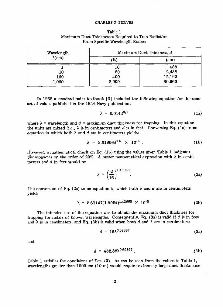
As early as 1948, Dr. H. G. Booker [1], an English scientist, gave an indication thatthere was a wavelength dependence for trapping radio energy into an elevated duct layer.However, no general equations were given at that time to show a mathematical relation-ship. In general, Dr. Booker's observation was that the greater the wavelength, thegreater the depth of the duct layer for trapping. In 1954, a U.S. Navy meteorologicalpublication [2] contained a table, consisting of four entries, that gave the maximumwavelength as a function of duct height, but again no general equation was given tosatisfy the entries in the table (Table 1 of this report).

Note: Manuscript submitted January 29, 1974.

1

CHARLES G. PURVES

Table 1Maximum Duct Thicknesses Required to Trap Radiation

From Specific Wavelength Radars

Wavelength Maximum Duct Thickness, d

X(cm) (ft) | (cm)

1 16 48810 80 2,438

100 400 12,1921,000 2,000 60,960

In 1965 a standard radar textbook [3] included the following equation for the sameset of values published in the 1954 Navy publication:

X = 0.014d3/ 2 (la)

where X = wavelength and d = maximum duct thickness for trapping. In this equationthe units are mixed (i.e., X is in centimeters and d is in feet. Converting Eq. (la) to anequation in which both X and d are in centimeters yields:

X = 8.31966d'-5 X 10-5 . (lb)

However, a mathematical check on Eq. (lb) using the values given Table 1 indicatesdiscrepancies on the order of 20%. A better mathematical expression with X in centi-meters and d in feet would be

d 1.43068

\=16 . (2a)

The conversion of Eq. (2a) to an equation in which both X and d are in centimetersyields

X = 5.67147(1.905d)A 4 30 68 X 10-5 (2b)

The intended use of the equation was to obtain the maximum duct thickness fortrapping for radars of known wavelengths. Consequently, Eq. (3a) is valid if d is in feetand X is in centimeters, and Eq. (3b) is valid when both d and X are in centimeters:

d = 16X0.6 9 8 9 7 (3a)

and

d = 482.88X 0.6 9 8 9 7 . (3b)

Table 1 satisfies the conditions of Eqs. (3). As can be seen from the values in Table 1,wavelengths greater than 1000 cm (10 m) would require extremely large duct thicknesses

2

NRL REPORT 7725

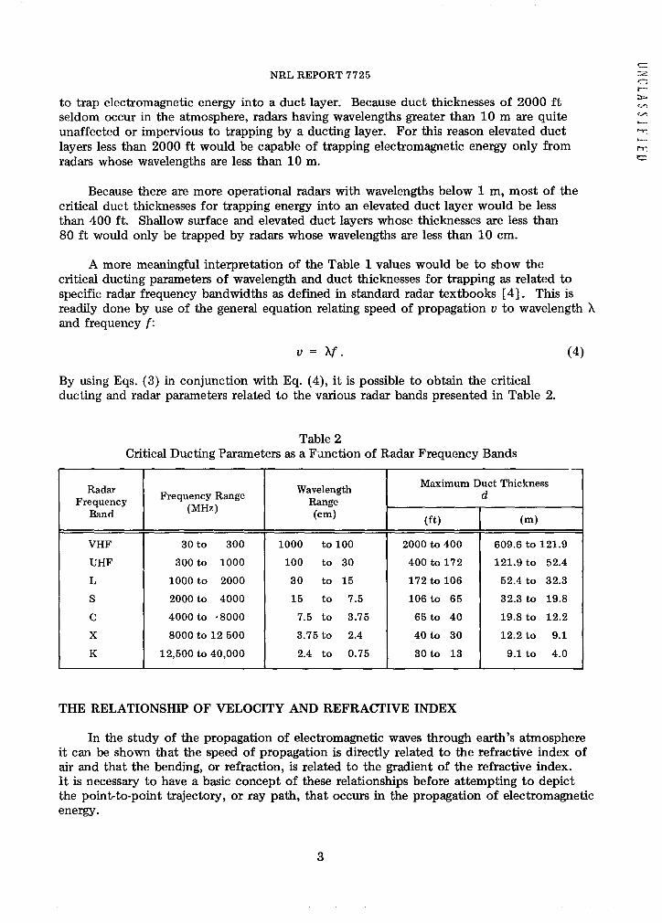
to trap electromagnetic energy into a duct layer. Because duct thicknesses of 2000 ftseldom occur in the atmosphere, radars having wavelengths greater than 10 m are quiteunaffected or impervious to trapping by a ducting layer. For this reason elevated ductlayers less than 2000 ft would be capable of trapping electromagnetic energy only fromradars whose wavelengths are less than 10 m.

Because there are more operational radars with wavelengths below 1 m, most of thecritical duct thicknesses for trapping energy into an elevated duct layer would be lessthan 400 ft. Shallow surface and elevated duct layers whose thicknesses are less than80 ft would only be trapped by radars whose wavelengths are less than 10 cm.

A more meaningful interpretation of the Table 1 values would be to show thecritical ducting parameters of wavelength and duct thicknesses for trapping as related tospecific radar frequency bandwidths as defined in standard radar textbooks [4]. This isreadily done by use of the general equation relating speed of propagation v to wavelength Xand frequency f:

v= V. (4)

By using Eqs. (3) in conjunction with Eq. (4), it is possible to obtain the criticalducting and radar parameters related to the various radar bands presented in Table 2.

Table 2Critical Ducting Parameters as a Function of Radar Frequency Bands

Maximum Duct ThicknessRadar Frequency Range Wavelength dFrequency 'z'Range_______

Band (MHz) (cm)

VHF 30 to 300 1000 to 100 2000 to 400 609.6 to 121.9

UHF 300 to 1000 100 to 30 400 to 172 121.9 to 52.4

L 1000 to 2000 30 to 15 172 to 106 52.4 to 32.3

S 2000 to 4000 15 to 7.5 106 to 65 32.3 to 19.8

C 4000 to -8000 7.5 to 3.75 65 to 40 19.8 to 12.2

X 8000 to 12 500 3.75 to 2.4 40 to 30 12.2 to 9.1

K 12,500 to 40,000 2.4 to 0.75 30 to 13 9.1 to 4.0

THE RELATIONSHIP OF VELOCITY AND REFRACTIVE INDEX

In the study of the propagation of electromagnetic waves through earth's atmosphereit can be shown that the speed of propagation is directly related to the refractive index ofair and that the bending, or refraction, is related to the gradient of the refractive index.It is necessary to have a basic concept of these relationships before attempting to depictthe point-to-point trajectory, or ray path, that occurs in the propagation of electromagneticenergy.

3

CHARLES G. PURVES

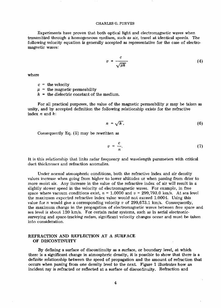
Experiments have proven that both optical light and electromagnetic waves whentransmitted through a homogeneous medium, such as air, travel at identical speeds. Thefollowing velocity equation is generally accepted as representative for the case of electro-magnetic waves:

cv = N/p-k (4)

where

c = the velocityp = the magnetic permeabilityk = the dielectric constant of the medium.

For all practical purposes, the value of the magnetic permeability p may be taken asunity, and by accepted definition the following relationship exists for the refractiveindex n and k:

n = A4F. (6)

Consequently Eq. (5) may be rewritten as

c=. (7)n

It is this relationship that links radar frequency and wavelength parameters with criticalduct thicknesses and refraction anomalies.

Under normal atmospheric conditions, both the refractive index and air densityvalues increase when going from higher to lower altitudes or when passing from drier tomore moist air. Any increase in the value of the refractive index of air will result in aslightly slower speed in the velocity of electromagnetic waves. For example, in freespace where vacuum conditions exist, n = 1.0000 and v = 299,793.0 km/s. At sea levelthe maximum expected refractive index value would not exceed 1.0004. Using thisvalue for n would give a corresponding velocity v of 299,673.1 km/s. Consequently,the maximum change in the propagation of electromagnetic waves between free space andsea level is about 120 km/s. For certain radar systems, such as in aerial electronic-surveying and space-tracking radars, significant velocity changes occur and must be takeninto consideration.

REFRACTION AND REFLECTION AT A SURFACEOF DISCONTINUITY

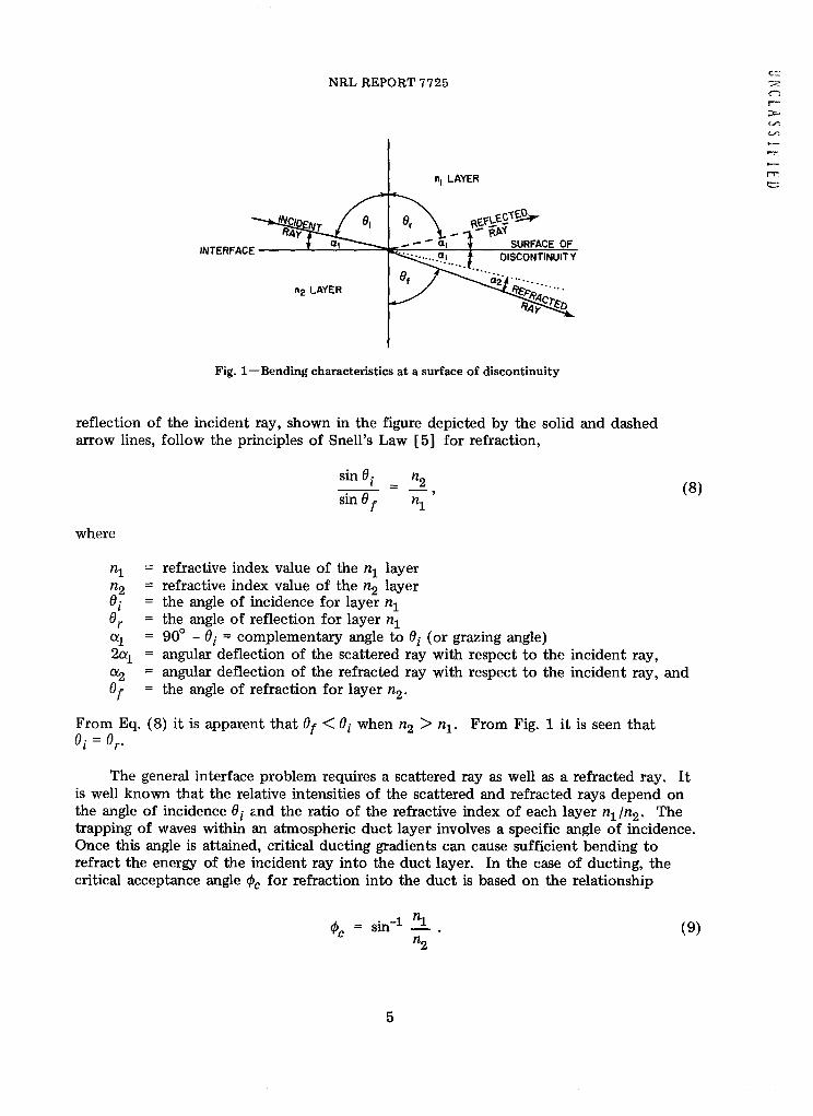
By defining a surface of discontinuity as a surface, or boundary level, at whichthere is a significant change in atmospheric density, it is possible to show that there is adefinite relationship between the speed of propagation and the amount of refraction thatoccurs when passing from one density level to the next. Figure 1 illustrates how anincident ray is refracted or reflected at a surface of discontinuity. Refraction and

4

NRL REPORT 7725

n, LAYER

INTERFACE '. ~ ~ ~ ~DISCONTINUITY

n2 LAYER

Fig. 1-Bending characteristics at a surface of discontinuity

reflection of the incident ray, shown in the figure depicted by the solid and dashedarrow lines, follow the principles of Snell's Law [5] for refraction,

sin Oi n2(8)

sin 0 nj

where

nj = refractive index value of the n1 layern2 = refractive index value of the n2 layerOi = the angle of incidence for layer njOr = the angle of reflection for layer n1a, = 900 - Oi = complementary angle to Oi (or grazing angle)2a, = angular deflection of the scattered ray with respect to the incident ray,% = angular deflection of the refracted ray with respect to the incident ray, andOf = the angle of refraction for layer n2.

From Eq. (8) it is apparent that Of < Oi when n2 > n1. From Fig. 1 it is seen thatOi = or.

The general interface problem requires a scattered ray as well as a refracted ray. Itis well known that the relative intensities of the scattered and refracted rays depend onthe angle of incidence Oi and the ratio of the refractive index of each layer nl /n2 . Thetrapping of waves within an atmospheric duct layer involves a specific angle of incidence.Once this angle is attained, critical ducting gradients can cause sufficient bending torefract the energy of the incident ray into the duct layer. In the case of ducting, thecritical acceptance angle kc for refraction into the duct is based on the relationship

a = sin-' nj (9)

5

CHARLES G. PURVES

For all practical considerations the ratio nj /n2 t 1; therefore, the critical acceptanceangle Oc ; 10. In terms of the diagram in Fig. 1, trapping occurs when the grazing anglea, is equal to Oc Therefore the critical incidence angle Oi to refract the incident rayinto the duct is the complement of the critical grazing angle a, is 890. Consequently,only rays launched nearly parallel (within 10) of the duct interface level, or duct axis,are trapped. Therefore, the amount of refraction, or bending, to get into the duct layeris not very large. Once ducting occurs, the rays will continue to remain in the ductlayer as long as a ducting gradient exists between layers n1 and n2. After trapping occurs,the principal relationship that keeps the ray path in the n2 layer where ducting occursis primarily governed by the laws of reflection.

According to total reflection theory, radiation in a more dense medium (n2 layer)meeting the boundary of a less dense medium (n1 layer) at an angle greater than thecritical angle will be totally reflected back into the more dense medium where n2 > n1 .For this reason, once the radient energy is refracted into the more dense n2 layer,the rays are continually contained in the duct layer by reflection at the duct interfaceas long as a trapping refractive index gradient exists. The principles of total reflectiontheory help to explain why low-energy output transmitters are capable of transmittingmeasurable signals via an elevated duct layer for hundreds and at times thousands ofmiles beyond the normal radar horizon ranges with virtually no signal losses.

The speed of electromagnetic wave propagation in layers n1 and n2 is

cV, = - (10)

nl

and

cv -* (11)2 n2

THE REFRACTIVE INDEX EQUATION

The magnitude of the refractive index of air n has a rather small range of fromunity, in free space, to approximately 1.0004 at sea level. In radar meteorology it ismore convenient to facilitate numerical computations of n as follows:

N = (n - 1)106 . (12)

This version is sometimes referred to as the "refractivity" index; computed values of Nare commonly referred to as N units. Values of N units can be numerically computedas a function of standard meteorological parameters where the general equation for Ntakes the form

N = A (P + Be) (13)

6

NRL REPORT 7725

where

T = Kelvin temperatureP = total atmospheric pressure (in millibars)e = vapor pressure (in millibars).

The values of constants A and B have been investigated many times by scientificexperiments. The National Bureau of Standards endorses the statistical evaluation ofSmith and Weintraub [6], as published in 1953, where A = 77.6 and B = 4810. In-sertion of these constants into the general equation for N gives

N = 77.6 - + (3.73 X >( 5) e (14)

where the first term is generally referred to as the "dry" air term and the second termthe "moist" or "wet" air term of the refractive index equation.

The refractive index equation N as shown in Eq. (14) has the general mathematicalform of a second-degree polynominal equation. To visualize the effect each of the meteoro-logical parameters P, T, and e has on the refractive index equation N, it is necessary todetermine their respective partial differential equations. The following set of partial differ-ential equations is presented to show how a unit change in pressure P, temperature T, andvapor pressure e affects the value of N:

aN 77.6 (15)aJP T'(5

aN _ -77.6 (p 9613.4e\aT T2 '(6

and

3N 373 000-e (17)

In the above equations it can be seen that all of the partial derivatives have a temperaturedependence. The partial derivatives of Eqs. (15) and (17) depend only upon the temperature,whereas in Eq. (16) the partial derivative aN/3T is a function of all three meteorological pa-rameters P. T, and e. Table 3 is presented to show the respective N unit changes that occurdue to a unit change in arbitrarily selected values of pressure, temperature and vapor pressure.The tabular values presented in Table 3 are representative of typical maximum and minimumatmospheric conditions one would expect in regions where ducting normally occurs. Inspec-tion of the partial derivatives obtained for the representative maximum and minimum casesindicates negligible differences of less than 1 N unit. Consequently, the average derivativescan be evaluated to see what significant relationship exists between them. For example,the approximate average value of

7

CHARLES G. PURVES

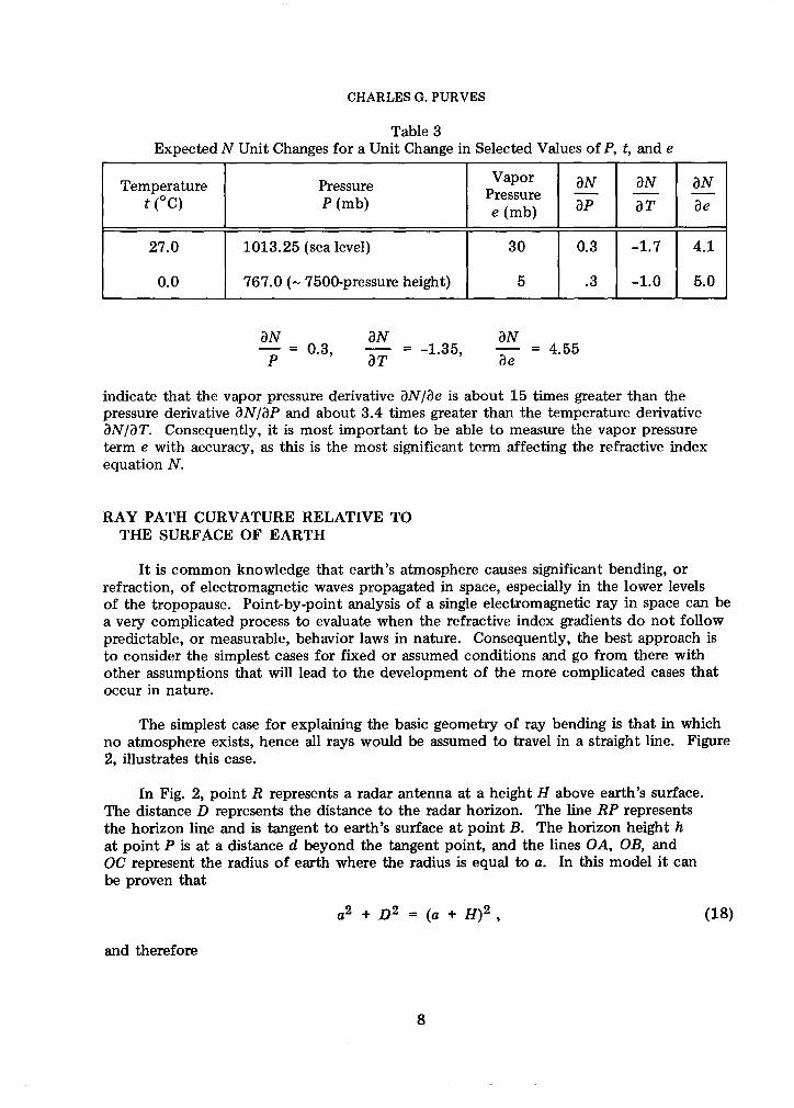
Table 3Expected N Unit Changes for a Unit Change in Selected Values of P, t, and e

Temperature Pressure Vapor 3N I aN aNt (0C) P (mb) e (mb) aP aT ae

27.0 1013.25 (sea level) 30 0.3 -1.7 4.1

0.0 767.0 (- 7500-pressure height) 5 .3 -1.0 5.0

aN aN aNN = 0.3,' aN = -1.35, aN = 4.55

indicate that the vapor pressure derivative aNlae is about 15 times greater than thepressure derivative aN/aP and about 3.4 times greater than the temperature derivativeaNlaT. Consequently, it is most important to be able to measure the vapor pressureterm e with accuracy, as this is the most significant term affecting the refractive indexequation N.

RAY PATH CURVATURE RELATIVE TOTHE SURFACE OF EARTH

It is common knowledge that earth's atmosphere causes significant bending, orrefraction, of electromagnetic waves propagated in space, especially in the lower levelsof the tropopause. Point-by-point analysis of a single electromagnetic ray in space can bea very complicated process to evaluate when the refractive index gradients do not followpredictable, or measurable, behavior laws in nature. Consequently, the best approach isto consider the simplest cases for fixed or assumed conditions and go from there withother assumptions that will lead to the development of the more complicated cases thatoccur in nature.

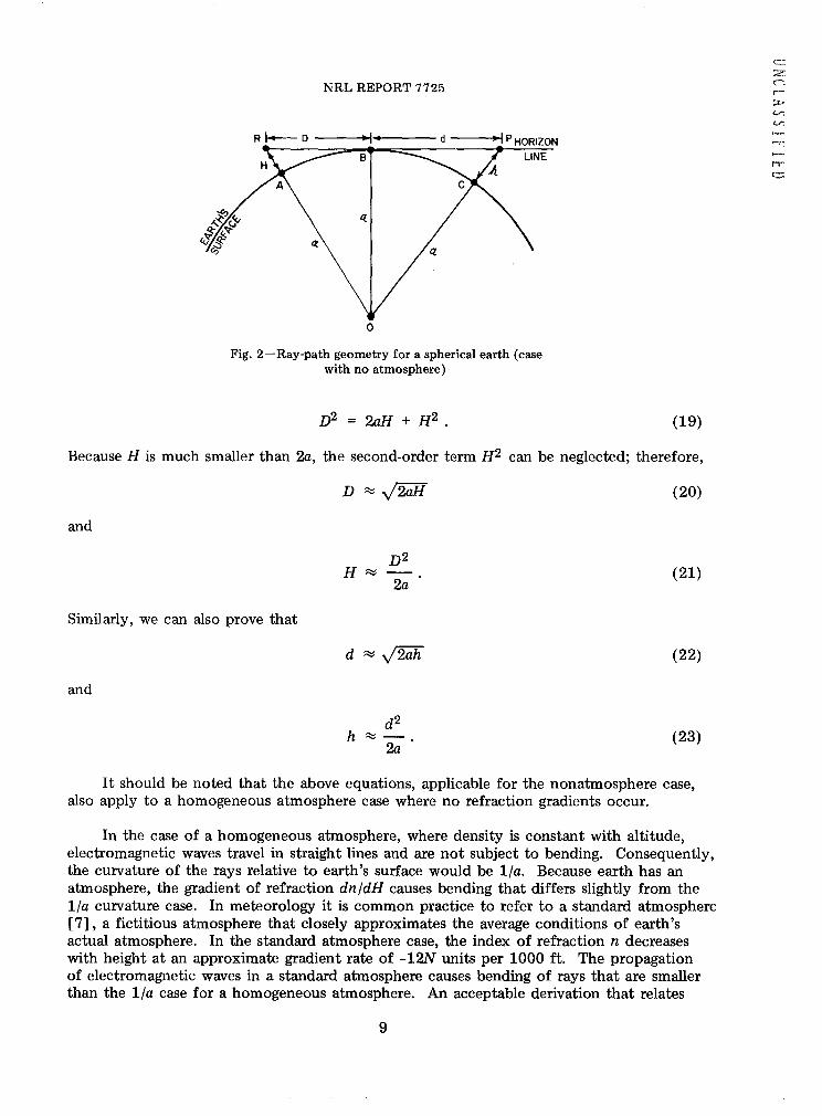
The simplest case for explaining the basic geometry of ray bending is that in whichno atmosphere exists, hence all rays would be assumed to travel in a straight line. Figure2, illustrates this case.

In Fig. 2, point R represents a radar antenna at a height H above earth's surface.The distance D represents the distance to the radar horizon. The line RP representsthe horizon line and is tangent to earth's surface at point B. The horizon height hat point P is at a distance d beyond the tangent point, and the lines OA, OB, andOC represent the radius of earth where the radius is equal to a. In this model it canbe proven that

a2 + D2 = (a + H)2 (18)

and therefore

8

NRL REPORT 7725

0

Fig. 2-Ray-path geometry for a spherical earth (casewith no atmosphere)

D2 = 2aH + H2 . (19)

Because H is much smaller than 2a, the second-order term H2 can be neglected; therefore,

D -/-fa (20)

and

D2H -- . (21)

2a

Similarly, we can also prove that

d e/-2a (22)

d2h ;t-2.2a

(23)

It should be noted that the above equations, applicable for the nonatmosphere case,also apply to a homogeneous atmosphere case where no refraction gradients occur.

In the case of a homogeneous atmosphere, where density is constant with altitude,electromagnetic waves travel in straight lines and are not subject to bending. Consequently,the curvature of the rays relative to earth's surface would be 1/a. Because earth has anatmosphere, the gradient of refraction dn/dH causes bending that differs slightly from the1/a curvature case. In meteorology it is common practice to refer to a standard atmosphere[7], a fictitious atmosphere that closely approximates the average conditions of earth'sactual atmosphere. In the standard atmosphere case, the index of refraction n decreaseswith height at an approximate gradient rate of -12N units per 1000 ft. The propagationof electromagnetic waves in a standard atmosphere causes bending of rays that are smallerthan the 1/a case for a homogeneous atmosphere. An acceptable derivation that relates

9

C=

:2-1

r-:;r-I-, �,1_`�

rr.cl_-

and

CHARLES G. PURVES

the curvature of a ray relative to earth's surface for actual atmospheric conditions in-dicates that the bending relationship adheres to the following equation [8]:

dq5 1 dn-= - + d (24)ds R dh

where

0 = the bending angles = distanceR = radius of earth, a.

From Eq. (24) it can be shown that in the actual atmosphere where dn/dhdecreases with height, a ray path that is concentric, or parallel, to earth's curvature meetsthe criteria

1 -dna = h - '(25)a Ah

Under actual refraction conditions in the atmosphere, trapping (or ducting) conditionsoccur only when the angle of the ray is within 10 of being parallel to earth's curvature.Rays whose angles are greater than 10 from earth's horizon normally penetrate rightthrough a ducting layer. Consequently, for trapping to occur, both the magnitude of thebending angle 0 and the refractive index gradient dn/dh must adhere to critical limits.The critical angle q5 has already been defined as being about 10. Equation (25) alsosatisfies the conditions for the critical refractive index gradient dn/dh that would causetrapping and cause the ray path to parallel earth's curvature. For convenience, we expressearth's curvature in feet, refractive index as N, and the gradient dN/dh in N units per1000 ft, where

dN =Nh2 Nhi (26)

and

dh = hi. (27)

Standard Mathematical Tables [9] gives the mean radius of earth as 3959 mi. The con-version from miles to feet would give the mean radius of earth as

-20.9 X 106 ft, or a : 20.9 X 106 ft. (28)

Because N has been defined as being equal to (n - 1)106, the conversion of the refrac-tive index gradient in terms of N units becomes

dn -dN_n = _N 1O-6 (29)

If Eqs. (26) through (29) are used, Eq. (25) can be rewritten as

10

NRL REPORT 7725

1 tNh Nh\1 = _ h2 hi) 10-6 (30)

20.9(10)6 \ h2 - h(

or

Nh2 Nh 1 = -0.04785. (31)h2 hi al20.9

Equation (31) now represents the critical refractive index gradient (dN/dh) for trappingwhere

/ dN\d)- 0.048. (32)dh /

For convenience, when this gradient is expressed in terms of N units per 1000 ft, wehave

(dN) - -48N units per 1000 ft. (33)

Consequently, whenever a negative refractive index gradient of 48N units per 1000 ftoccurs, trapping can be expected for the rays within 10 of the layer of discontinuity.

A CLASSIFICATION SYSTEM FOR REFRACTION

The gradient change of the index of refraction N under normal atmospheric con-ditions can be evaluated in both the horizontal and vertical directions. The most persis-tent and strongest gradients are normally associated with the vertical profiles of N, if oneconsiders the mesoscale or macroscale fields. However, it should be noted that whenstrong ducting gradients of dN/dh are observed, there may be a flat wavy undulation ofthe duct layer. Consequently, strong refractive gradients, normally associated with agradient height relationship, cap also be measured in the horizontal field if one takes themicroscale field into account.

The Navy has adopted a general classification system [10] of identifying atmosphericrefractive index gradients, mainly for forecasting and climatological purposes. The sys-tem identifies four separate categories of refractive index gradients:

1. Subrefraction-N increases with height. Rays curve upward with reference to astraight line (opposite in direction to the curvature of earth's surface). Radioand radar ranges are significantly reduced; occurrence is quite rare.

2. Normal-N decreases with height; the range of dN/dh per 1000 ft is from 0 to24. Rays curve downward (in the same direction as the curvature of earth'ssurface) but not as sharply as those in the superrefraction case. Radio andradar performance is generally undisturbed.

11

CHARLES G. PURVES

3. Superrefraction-N decreases with height; the range of dN/dh per 1000 ft isfrom 24 to 48. Rays curve downward (in the same direction as the curvatureof earth's surface) more sharply than those in the normal refraction case butnot as sharply as earth's surface. Radio and radar ranges are significantly ex-tended; occurrence is quite frequent.

4. Trapping-N decreases with height; the range of dN/dh per 1000 ft is greaterthan 48. Rays curve downward more sharply than the curvature of earth'ssurface. Radio and radar performance is greatly disturbed (e.g., ranges areextended greatly and radar holes appear); occurrence is not frequent.

AREAS OF THE WORLD WITH PERSISTENTOCEANIC DUCTING CONDITIONS

The two most significant large-scale meteorological phenomena that cause thetrapping of electromagnetic waves into an effective atmospheric waveguide are related tothe trade wind temperature inversion and large-scale subsidence. Strong and persistentelevated duct layers over at least one-third of the surface of the oceans are commonlyobserved throughout the year.

The principal source region of the trade wind inversion is normally on the westcoast side of continents, usually close to mountain ranges. Enhancement of the strengthof the temperature inversion is related to the downslope gravity winds that heat and drythe air as it flows from the mountains to the seas. Such winds are sometimes locallyreferred to by such names as Foehn, Santa Ana and Chinook winds. Within severalhundred miles of coastal areas such as California, Chile, Southwest Africa, and Angola,where the trade wind inversion originates, the normally elevated duct layers associatedwith the temperature inversion layer may at times extend to the surface. In all of theseprincipal source regions of the trade wind inversion, the large-scale flow follows thecoastline toward the Equator and then flows from the continents in an easterly directionon both sides of the Equator. This easterly trade wind circulation follows the bottomside of large oceanic high-pressure cells in the Northern Hemisphere and the top side ofhighs in the Southern Hemisphere. The strength of the trade wind inversion weakensin the downstream direction. As it weakens it also rises. Consequently, there normallyis a relationship between temperature inversion height and the magnitude of the tradewind inversion.

Large-scale subsidence is associated with high-pressure areas. Large, permanent-high-pressure cells dominate the surfaces of the oceans in both hemispheres between the 150and 450 latitude belts. In the summer months, in both hemispheres, there is a 50 to100 poleward shift of these large oceanic high-pressure cells. These cells play a majorrole in the steerage of global frontal weather storm systems in that they block and deterthe penetration of frontal weather, which keeps the major storm tracks to the polewardside of the high. The statistically stable characteristics normally associated with highpressures are those of good weather conditions, generally weak winds and clear skies inthe center, and low stratus clouds around the peripheral regions. These characteristics arethe result of large-scale subsidence, which produces significant temperature inversionsand results in strong ducting gradients to form above the base of the inversion.

12

NRL REPORT 7725

Standard worldwide atlas presentations of radio refractivity conditions are generallybased on radiosonde measurements of pressure, temperature, and humidity. The slowresponse time of these instruments masks the full-scale detection of these parameters,which limits the interpretation of refractive index gradients. As a result, the statisticalanalysis portraying the frequency of occurrences for ducting gradients in the atmospherecontains values that are far too low, perhaps by as much as a factor of 5 to 10. Toshow appropriate statistics, the observed data must be measured by fast-response instru-ments whose lag times are on the order of 0.01 s or faster. The microwave refractometeris a fast-response instrument that measures the refractive index of air directly, rather thandetermining it indirectly through measurements of P, t, and e and allows for reliablemeasurements of the significant ducting refractive index gradients.

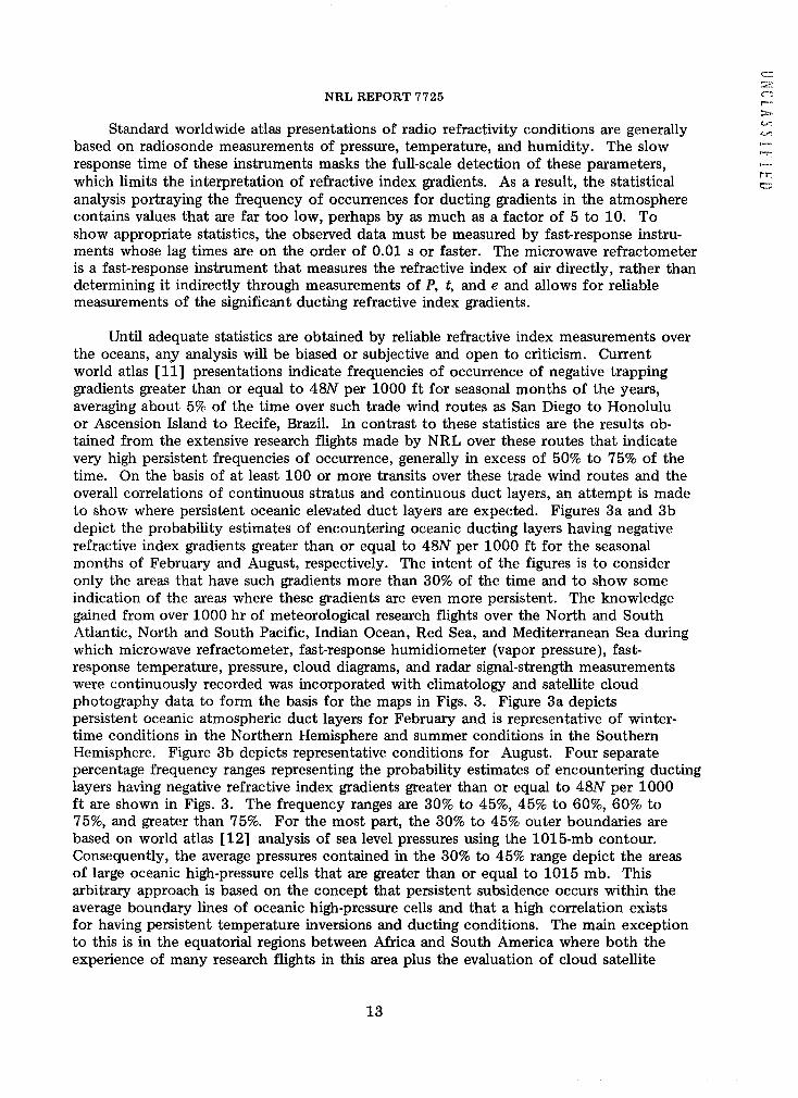
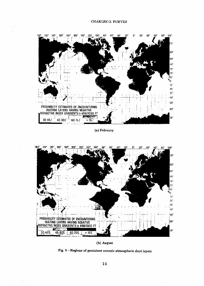
Until adequate statistics are obtained by reliable refractive index measurements overthe oceans, any analysis will be biased or subjective and open to criticism. Currentworld atlas [11] presentations indicate frequencies of occurrence of negative trappinggradients greater than or equal to 48N per 1000 ft for seasonal months of the years,averaging about 5% of the time over such trade wind routes as San Diego to Honoluluor Ascension Island to Recife, Brazil. In contrast to these statistics are the results ob-tained from the extensive research flights made by NRL over these routes that indicatevery high persistent frequencies of occurrence, generally in excess of 50% to 75% of thetime. On the basis of at least 100 or more transits over these trade wind routes and theoverall correlations of continuous stratus and continuous duct layers, an attempt is madeto show where persistent oceanic elevated duct layers are expected. Figures 3a and 3bdepict the probability estimates of encountering oceanic ducting layers having negativerefractive index gradients greater than or equal to 48N per 1000 ft for the seasonalmonths of February and August, respectively. The intent of the figures is to consideronly the areas that have such gradients more than 30% of the time and to show someindication of the areas where these gradients are even more persistent. The knowledgegained from over 1000 hr of meteorological research flights over the North and SouthAtlantic, North and South Pacific, Indian Ocean, Red Sea, and Mediterranean Sea duringwhich microwave refractometer, fast-response humidiometer (vapor pressure), fast-response temperature, pressure, cloud diagrams, and radar signal-strength measurementswere continuously recorded was incorporated with climatology and satellite cloudphotography data to form the basis for the maps in Figs. 3. Figure 3a depictspersistent oceanic atmospheric duct layers for February and is representative of winter-time conditions in the Northern Hemisphere and summer conditions in the SouthernHemisphere. Figure 3b depicts representative conditions for August. Four separatepercentage frequency ranges representing the probability estimates of encountering ductinglayers having negative refractive index gradients greater than or equal to 48N per 1000ft are shown in Figs. 3. The frequency ranges are 30% to 45%, 45% to 60%, 60% to75%, and greater than 75%. For the most part, the 30% to 45% outer boundaries arebased on world atlas [12] analysis of sea level pressures using the 1015-mb contour.Consequently, the average pressures contained in the 30% to 45% range depict the areasof large oceanic high-pressure cells that are greater than or equal to 1015 mb. Thisarbitrary approach is based on the concept that persistent subsidence occurs within theaverage boundary lines of oceanic high-pressure cells and that a high correlation existsfor having persistent temperature inversions and ducting conditions. The main exceptionto this is in the equatorial regions between Africa and South America where both theexperience of many research flights in this area plus the evaluation of cloud satellite

13

CHARLES G. PURVES

100° 120 140° 160° 180° 160° 1408

P~ROBABILITY ESTIMATES OF ENCOUNTERINGDUCTING LAYERS HAVING NEGATIVE

REREFRACTIVEIINEX GRADIENTS >48N/1000 FT

30 45 4560 60) ',I 7

(a) February

140° 160° 180° 160° 140° 120°

PROBABILITY ESTIMATES OF ENCOUNTERING__j DUCTING LAYERS HAVING NEGATIVE -

REFRACTIVE INDEX GRADIENTS ~ 48N/1000 FT 4

Ft --- ____ 3 -~

3bO46i 456D _ 5

. ..... &P ......__q..75%

(b) August

Fig. 3-Regions of persistent oceanic atmospheric duct layers

14

A, H,,..

J~~~~~~A I_ ~~~~~~~~30

- . . . . . . . .

- ^- I- '-^----^ - 150,T1 -u- 60° i~

,�. , . I I I � Ii I II--al. - ; I� I (

I,-----"- I 'iI

A 7_

NRL REPORT 7725

photography gave indications of high persistent trapping layers. The analysis of theprobability estimates greater than 50% is subjective and is based on the interpretation ofcloud satellite photography data gathered over a period of more than 4 years and the highcorrelation of cloud-type and ducting conditions observed during extensive researchinvestigations in trade wind areas.

ANOMALOUS PROPAGATION

Refraction effects, such as those associated with an elevated duct layer, especiallyfor radars scanning within a few degrees of the horizon, have both favorable andunfavorable military operational significance. The extended ranges resulting from ducting,at times hundreds of miles beyond the normal radar horizon, can be useful in the earlydetection of targets that under normal refraction conditions would not be seen. Thisfavorable aspect of early target detection via an elevated duct layer is also characterizedby a radar hole above the duct; consequently, radar targets within the radar hole goundetected. The presence of a radar hole can be either favorable or unfavorable from amilitary point of view. The favorable aspect is the ability to stay in the radar hole toavoid detection by enemy radars. The most important factor, from a strategic combatpoint of view, is to be aware that both a duct layer and a radar hole exist and to usethis knowledge advantageously whenever possible. Many military operational radar sys-tems scan at preset ranges; the operator can switch from say a 200-mi sweep display to a100-, 50-, and 10-mi display and follow the target as it moves closer to the observingradar. This aspect is fine in terms of giving an enlarged display much like a zoom cameralens. However, under ducting conditions, targets may be coming from multiple distancesbeyond that indicated on a fixed-sweep display scope. When this happens, false interpreta-tion of the individual radar target returns occurs, which in the past has caused mockbattle situations where long-range naval guns have fired at nonexistent targets beyond thevisual line-of-sight ranges. To avoid such situations, a radar must be able to discriminatebetween real and false ranges, a task that can only be done by measuring the travel timeto each target and showing the true ranges of each target displayed on the radar scopewithout ambiguity.

When anomalous propagation conditions such as ducting occur, it has been shownthat a negative refractive index gradient greater than or equal to 48N units per 1000 ftexists. What has not been discussed are examples in nature that cause the trappinggradients. In general, when there is a significant moisture discontinuity, temperatureinversion, or a combination of both, a corresponding density and refractive index gradientresults. Meteorological conditions that cause trapping gradients are often related to suchthings as large-scale subsidence, cloud formations, haze layers, divergence, gravity winds,advection, and evaporation.

Large-scale subsidence, or slow sinking of air, is associated with high-pressure areas.Over the oceans, large high-pressure cells may remain stationary for long periods of time.Typical weather associated with the center of large oceanic high-pressure cells is usuallyclear skies, light winds, and good visibilities except in low-level haze or fog layers. Thegeneral sinking of air from high altitudes results in adiabatic heating due to compression,and a decrease in moisture content. Normally, air temperature decreases with height at anapproximate rate of 20 C per 1000 ft. The adiabatic heating produced by the sinking air

15

CHARLES G. PURVES

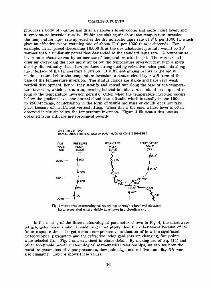
produces a body of warmer and drier air above a lower cooler and more moist layer, anda temperature inversion results. Within the sinking air above the temperature inversionthe temperature lapse rate approaches the dry adiabatic lapse rate of 30C per 1000 ft, whichgives an effective excess warming rate of about 10 C per 1000 ft as it descends. Forexample, an air parcel descending 10,000 ft at the dry adiabatic lapse rate would be 100warmer than a similar air parcel that descended at the standard lapse rate. A temperatureinversion is characterized by an increase of temperature with height. The warmer anddrier air overriding the cool moist air below the temperature inversion results in a sharpdensity discontinuity that often produces strong ducting refractive index gradients alongthe interface of the temperature inversion. If sufficient mixing occurs in the moistmarine stratum below the temperature inversion, a stratus cloud layer will form at thebase of the temperature inversion. The stratus clouds are stable and have very weakvertical development; hence, they stratify and spread out along the base of the tempera-ture inversion, which acts as a suppressing lid that inhibits vertical cloud development aslong as the temperature inversion persists. Often when the temperature inversion occursbelow the gradient level, the normal cloud-base altitude, which is usually in the 1500-to 2500-ft range, condensation in the form of visible moisture or clouds does not takeplace because of insufficient vertical lifting. When this is the case, a haze layer is oftenobserved in the air below the temperature inversion. Figure 4 illustrates this case asobtained from airborne meteorological records.

DATE: 19 DEC 1960RANGE: ABOUT 186 n.mi. WSW OF POINT MUGU AT 0049 Z (1649 PST)

TIME PRESSURE REFRACTIVE TEMPERATURESCALE HEIGHT INDEX SCALE(min) SCALE SCALE (IC)

(ft) (N)21.20

0050- 600 275

20.5'1600 4276

0049- 400 28

f 250 13.8 33114.0

100 X3410048-

Fig. 4-Airborne meteorological recordings through a low-level elevatedlayer associated with a visible haze layer in a cloudless sky

In the sensing of the three meteorological parameters shown in Fig. 4, the microwaverefractometer trace is much broader and more jittery than the other traces because of itsfaster response time. To get a more comprehensive evaluation of how the significantmeteorological parameters and the refractive index gradients are changing, five pointswere selected from Fig. 4 and examined in closer detail. By making use of Eq. (14) andother acceptable proven meteorological mathematical relationships, we can see how themoisture parameters of vapor pressure e, dew point tDp, and relative humidity RH werealso changing. Table 4 shows these values.

16

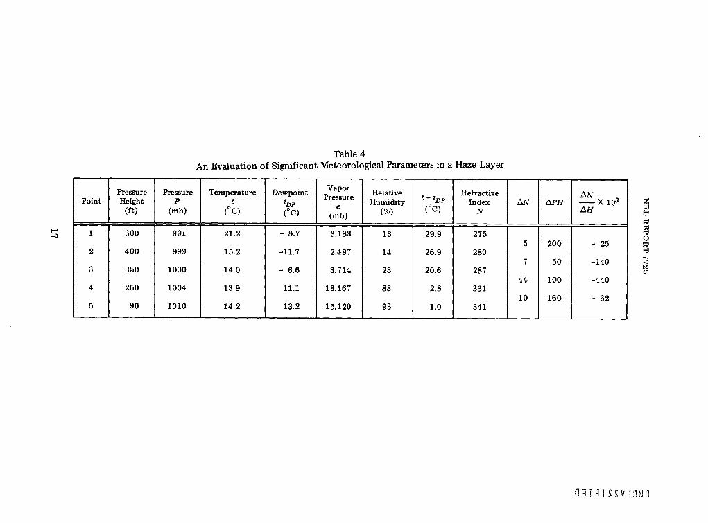
Table 4An Evaluation of Significant Meteorological Parameters in a Haze Layer

Pressure Pressure Temperature Dewpoint Vapor Relative t t Refractive ANPoint Height P t tDP e Humidity 'DP Index AN APHX 103

(ft) (mb) (0C) (C) (mb) ( ( C) N AH

1 600 991 21.2 - 8.7 3.183 13 29.9 275

2 400 999 15.2 -11.7 2.497 14 26.9 280

7 50 -1403 350 1000 14.0 - 6.6 3.714 23 20.6 287

44 100 -4404 250 1004 13.9 11.1 13.167 83 2.8 331

10 160 - 625 90 1010 14.2 13.2 15.120 93 1.0 341

I-'

z

10

01

C14 ' i IJ S s Y I1 N n

CHARLES G. PURVES

As can be seen from Table 4, the temperature inversion was over 70 C. The dramaticchange in relative humidity from 83% at the base of the temperature inversion (250 ft)to 23% at 100 ft above and to 13% at the 600 ft PH level illustrates how much the sub-siding air is dried out as it descends. The lower marine stratum, characterized by thevisible haze layer, has relative humidity values in the 83% to 93% range. The temperaturedepression difference t - tDp between the dry air temperature and the dewpoint tempera-ture has a minimum of 1.00 C in the haze and reaches a maximum of 29.90 C just a fewhundred feet above the base of the temperature inversion. From 400 to 600-ft PH asuperrefractive index gradient of -25 N per 1000 ft is observed. Below 400-ft PH, anegative trapping refractive gradient greater than 48N per 1000 ft is observed. Unfortunately,the aircraft could not safely go lower than 90-ft PH, so the refractive index gradient below90-ft PH is unobtainable. However, the evaluation of the haze layer from 250- to 90-ftPH implies that a trapping gradient may well exist. This gives rise to the general hypothesisthat oceanic evaporation (surface) ducts, which are generally believed to be quite shallowand normally less than 100 ft thick, may feed or be part of a low elevated duct layerthat is sometimes characterized by visible haze. The general ducting concept for surfaceoceanic evaporation ducts is that it is not particularly effective in extending the coverageof most shipboard radars because it is too shallow to trap most radar frequencies below3000 MHz, or wavelengths greater than 10 cm. As can be seen by the wavelengthdependence criteria for trapping shown in Table 2, most shipboard operational radars havingfrequencies greater than 300 MHz, or wavelengths less than 100 cm, would have beenable to trap energy into this duct layer.

On this particular research flight to observe meteorological and refraction conditionsalong the route from Honolulu to Point Mugu, the pilot's VOR was tuned to SantaCatalina on a VHF setting of 111.6 MHz at a range of 900 n.mi. Loud and clear audiosignals were received, indicating the existence of a strong elevated duct layer. The bestreception of the audio signal was received from an altitude just skimming the cloud topsto one 100 to 200 ft below the cloud tops. At the center of the interface of the tempera-ture inversion, which occurred about 100 ft above the cloud tops, the audio signals wouldcut out sharply. Several probes above and below the overcast stratus cloud layer, whosecloud tops were at 4300-ft PH and bases were at 3300-ft PH, resulted in loss of signal justabove the cloud tops and again at the cloud-base level. This showed agreement with themeteorological data because the duct and cloud thicknesses were both about 1000 ft. Theuse of the audio VOR signal is an independent verification that reliable deductions can bemade concerning expected duct heights, ranges, and thicknesses.

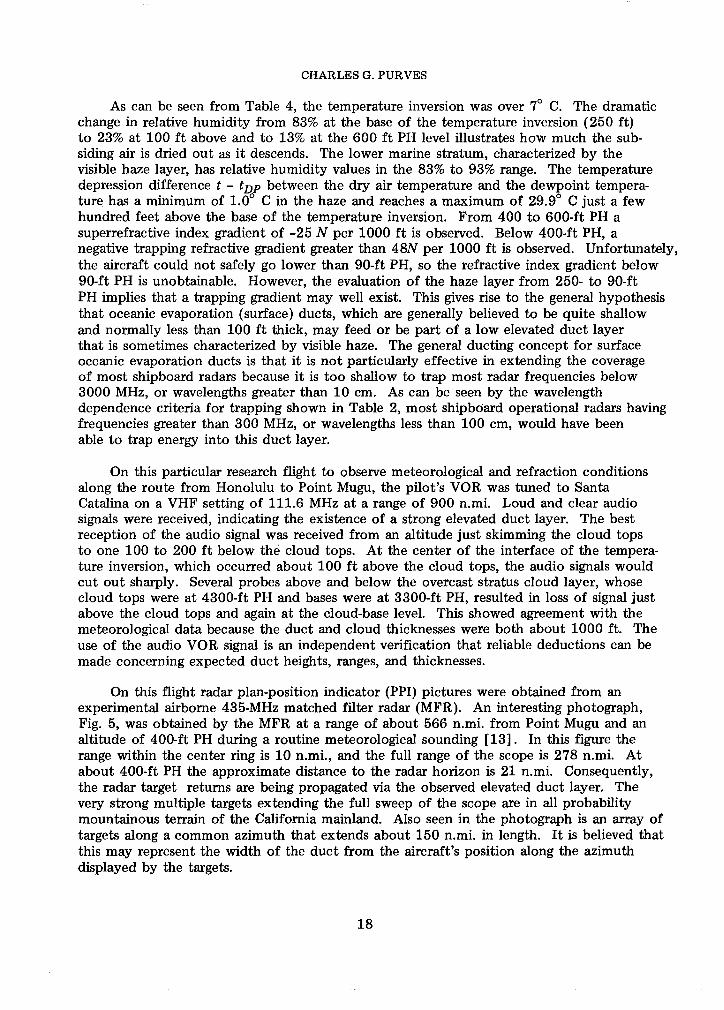
On this flight radar plan-position indicator (PPI) pictures were obtained from anexperimental airborne 435-MHz matched filter radar (MFR). An interesting photograph,Fig. 5, was obtained by the MFR at a range of about 566 n.mi. from Point Mugu and analtitude of 400-ft PH during a routine meteorological sounding [13]. In this figure therange within the center ring is 10 n.mi., and the full range of the scope is 278 n.mi. Atabout 400-ft PH the approximate distance to the radar horizon is 21 n.mi. Consequently,the radar target returns are being propagated via the observed elevated duct layer. Thevery strong multiple targets extending the full sweep of the scope are in all probabilitymountainous terrain of the California mainland. Also seen in the photograph is an array oftargets along a common azimuth that extends about 150 n.mi. in length. It is believed thatthis may represent the width of the duct from the aircraft's position along the azimuthdisplayed by the targets.

18

NRL REPORT 7725

Fig. 5-Target returns from beyond the radarhorizon via an elevated duct layer using a

~~ ~~ - .. , ~~~~ 435-MHz MFR system [13]

At 566 n.mi., a target on the MFR scope could appear either at the maximum rangelimit of 278 n.mi., which is the end of the second repetition period, or on the centercircle ring, at the start of the third repetition period (i.e., 10 + 278 + 278 = 566). Con-sequently the position of targets in close proximity of 566 n.mi. on the MFR scope maybe erroneously interpreted. For example, consider the case of two targets, A and B, thatare actually only 20 n.mi. apart where target A is at a true range from the aircraft of 550n.mi. and target B is 570 n.mi. from the aircraft along the same azimuth. The representa-tion of target A would then appear on the MFR scope at a range of 262 n.mi. andwould be in the second repetition period (i.e., 10 + 278 + 262 = 550). Target B wouldappear at an apparent range of 4 n.mi. from the 10-n.mi. center circle on the MFR scopeand would be in the third repetition period (i.e., 10 + 278 + 278 + 4 = 570). Con-sequently, the representation of targets A and B on the scope would falsely indicate therange difference between them as being 258 n.mi. when in reality they are 20 n.mi.apart. Other range ambiguities may also result when target reception occurs from anyother possible repetition period.

An NRL aircraft, during a 1960 Tradewinds III experiment, successfully recordedcontinuous signal-strength measurements via an elevated duct layer from a ground-basedradar at San Diego for a range of 2400 n.mi. to a point about 150 n.mi. past Honolulu,where the flight was terminated because of the range of the aircraft. The significance ofthis particular flight is to show that certain geographic regions of the world, wherepersistent ducts are observed, are capable of trapping electromagnetic waves and trans-porting them in an effective atmospheric waveguide, not for a few hundred miles beyondthe normal radar horizon but for several thousands of miles.

Detection of an atmospheric duct layer by audio VOR signals, when beyond thenormal radar horizon range for reception, can be correlated with visual cloud and hazelayer conditions and can be used to obtain independent estimates of duct height, range,and thickness. By using more than one VOR station, if possible, further estimates of

19

CHARLES G. PURVES

duct widths may be made. In the absence of meteorological refractive index data, itappears that audio VOR signals can provide an independent means for locating anddescribing significant characteristics of a duct layer. The same can be said of certainairborne radar systems such as the MFR.

It should be noted that most radar systems were designed to take into considerationthe estimated range to the horizon for normal atmospheric conditions and normalaircraft ceilings. For example, an aircraft at 40,000 ft would expect to have a radarhorizon range of about 213 n.mi. This explains why the typical range of operationalradars is about 200 n.mi. One approach to remove target range ambiguities in surfaceand elevated duct regions where the target return ranges exceed one repetition periodwould be to change the pulse repetition frequency (PRF) slightly. A switching back andforth at different PRFs would see no range changes of targets in the first repetitionperiod. For targets beyond the first repetition period, the change in PRF would helpidentify targets of ambiguous ranges as they would not appear at common ranges foreach of the PRF switch settings.

Until now the approach in obtaining a RIF has been by use of existing synopticmeteorological services where a forecaster would use whatever atmospheric data isavailable to him and by standard procedures make a forecast. This approach is stilldesirable; however, there are many additional aids to obtaining a RIF such as from air-craft radars, as already mentioned, plus the use of satellite cloud photographs where acorrelation of clouds and ducting layers may exist. By bringing to light some of thealternative methods not readily found in the literature of obtaining a RIF, we hope thatit may be possible for operational personnel in the field to obtain a RIF when thestandard forecasting service approach is unobtainable.

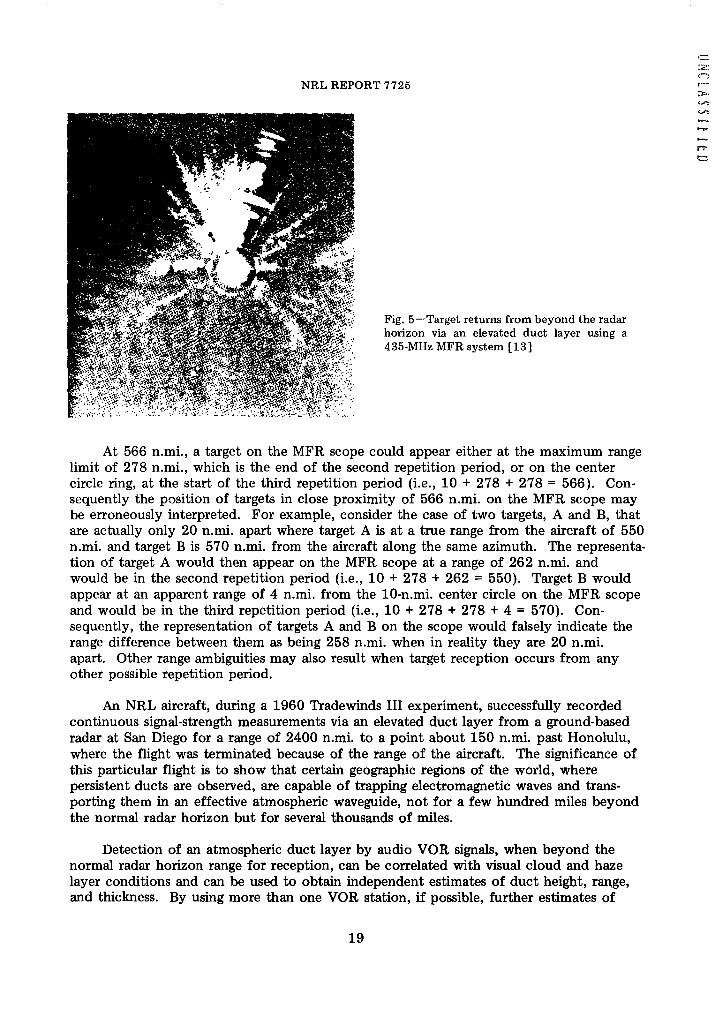
During a February 1961 Tradewind IV meteorological research flight over theHonolulu to San Diego route, a series of photographs of the MFR scope was obtainedabove, in, and below an elevated duct layer. A selection of 12 radar scope photographs[14] showing transhorizon radar returns associated with an elevated duct layer is presentedin Fig. 6.

During the 4.5-min span of the 12 photographs, the aircraft descended from 2660-to 560-ft PH and the range from San Diego changed from about 542 to 527 n.mi. Theradar scope pictures not only substantiate the presence of an elevated duct layer butclearly illustrate how target reception is affected in close proximity of the elevated ductlayer. During this flight the Navy Electronic Laboratory (NEL) at San Diego recordedsignal-strength measurements of the aircraft's 435-MHz MFR. A continuous duct layer,associated with a strong haze and thin scattered-to-broken stratus cloud layer, showedexcellent correlation with the microwave refractive index measurements and the recordingof the radar signal-strength measurements. The first detection of this continuous ductlayer by the NEL measurements occurred at a range of 1320 n.mi. In the last 550 n.mi.of this flight there was nearly lossless propagation with peak signals measured in the 25-to 30-dBm range. Photograph 1 in Fig. 6 was taken about 600 ft above the cloud topsand about 450 ft above the top of the duct as determined by refractometer data andvisual cloud observations. Here a faint but persistent target in the direction of flight(2 o'clock) is seen coming, presumably from the San Diego area. In the remainingphotographs the returns at 11 o'clock are presumed to be coming from the SanFrancisco area and the returns at 4 o'clock from Guadalupe Island. The azimuth spread

20

NRL REPORT 7725

1 2 3 4TIME 2306-10 TIME 2306-45 TIME 2307-13 TIME 2307-25

ALT 2660 ALT 2540 ALT 2375 ALT 2250RANGE 541.6 RANGE 540 RANGE 538 RANGE 537

5 6 7 8TIME 2308-05 TIME 2308-32 TIME 2308-57 TIME 2309-24

ALT 1880 ALT 1690 ALT 1500 ALT 1300RANGE 535 RANGE 534 RANGE 533 RANGE 531.5

9 10 11 12TIME 2309-36 TIME 2309-48 TIME 2310-28 TIME 2310-40

ALT 1200 ALT 1100 ALT 670 ALT 560RANGE 531 RANGE 530.5 RANGE 528 RANGE 5275

Fig. 6-Radar scope pictures associated with an elevated duct

of these targets is an indication that the duct is quite broad. Photographs 2 and 3 showslightly brighter illumination of the San Diego area targets and detection of targets fromthe San Francisco area. At the time of these photographs the aircraft was in clear airabout 200 to 300 ft above the duct base. Photograph 4, taken within 50 ft of the ducttop, shows many more returns from the San Diego area and a significant increase inillumination. Photographs 5, 6, and 7 were obtained within the duct layer, and thetargets show a high illumination, which indicates that the signal strength is greatestwithin the duct layer. This agrees with the recorded signal-strength measurements thatgave a peak reception power of 25 to 26 dBm when the aircraft was between 1900 and1000 ft. Photograph 10 was taken at 1100 ft, about 1150 ft below the duct top, andshows the San Diego returns to be fain although the San Francisco and GuadalupeIsland returns are somewhat stronger. Photograph 12 was taken at 560 ft, or about1700 ft below the duct top, and shows no target returns. The minimum detectablesignal-strength level for the 435-MHz MFR occurs near 100 dBm. Consequently a dropof about 80 dB, or more, is associated with the change from the peak signal strengthswithin the duct layer to the loss of signal below the duct layer.

21

CHARLES G. PURVES

CORRELATION OF ELEVATED DUCTS WITHCONTINUOUS CLOUD HAZE LAYERS

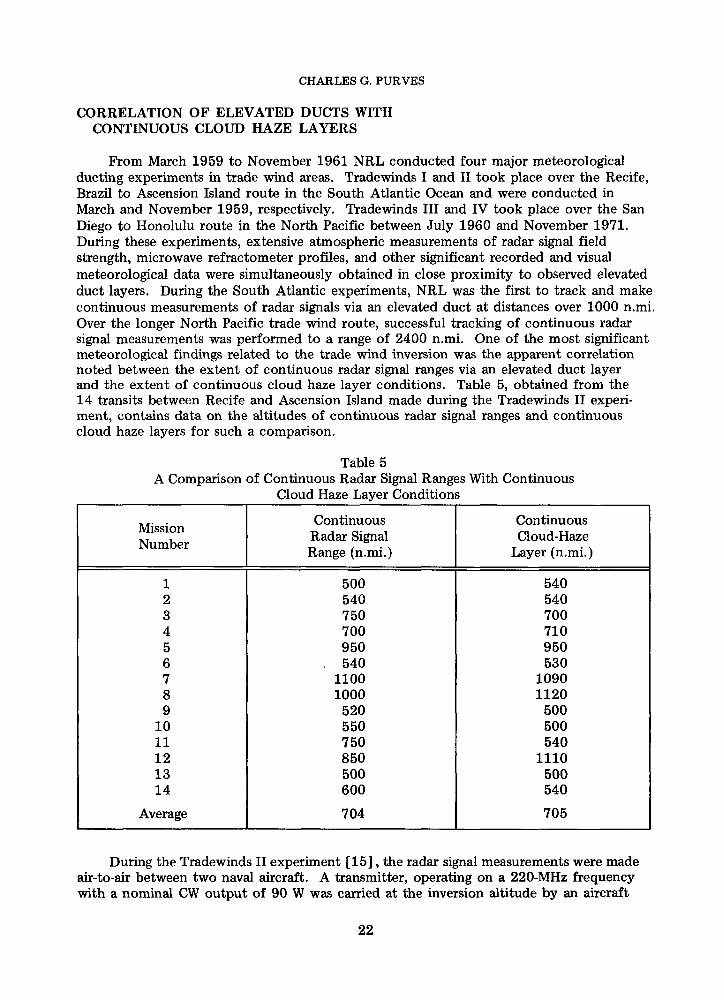
From March 1959 to November 1961 NRL conducted four major meteorologicalducting experiments in trade wind areas. Tradewinds I and II took place over the Recife,Brazil to Ascension Island route in the South Atlantic Ocean and were conducted inMarch and November 1959, respectively. Tradewinds III and IV took place over the SanDiego to Honolulu route in the North Pacific between July 1960 and November 1971.During these experiments, extensive atmospheric measurements of radar signal fieldstrength, microwave refractometer profiles, and other significant recorded and visualmeteorological data were simultaneously obtained in close proximity to observed elevatedduct layers. During the South Atlantic experiments, NRL was the first to track and makecontinuous measurements of radar signals via an elevated duct at distances over 1000 n.mi.Over the longer North Pacific trade wind route, successful tracking of continuous radarsignal measurements was performed to a range of 2400 n.mi. One of the most significantmeteorological findings related to the trade wind inversion was the apparent correlationnoted between the extent of continuous radar signal ranges via an elevated duct layerand the extent of continuous cloud haze layer conditions. Table 5, obtained from the14 transits between Recife and Ascension Island made during the Tradewinds II experi-ment, contains data on the altitudes of continuous radar signal ranges and continuouscloud haze layers for such a comparison.

Table 5A Comparison of Continuous Radar Signal Ranges With

Cloud Haze Layer ConditionsContinuous

During the Tradewinds II experiment [15], the radar signal measurements were madeair-to-air between two naval aircraft. A transmitter, operating on a 220-MHz frequencywith a nominal CW output of 90 W was carried at the inversion altitude by an aircraft

22

Mission Continuous Continuous

Number Radar Signal Cloud-HazeRange (n.mi.) Layer (n.mi.)

1 500 5402 540 5403 750 7004 700 7105 950 9506 . 540 5307 1100 10908 1000 11209 520 500

10 550 50011 750 54012 850 111013 500 50014 600 540

Average 704 705

NRL REPORT 7725

that flew a racetrack pattern 100 n.mi. off the beach at Recife. The receiver was carriedat the inversion level by another aircraft flying along the 1200-n.mi. route to AscensionIsland. It is interesting to note that the transmitted air-to-air signals were propagated themaximum range between the two aircraft on 3 of the 14 flights. Using the range valuesshown in Table 5 results in a high correlation of r = 0.92 when comparing the ranges ofthe continuous radar signals with the continuous cloud haze layers.

Further data that correlated the extent of radio signal experiments with the extent ofcontinuous cloud haze layers was noted during the North Pacific Tradewinds III and IVexperiments. These experiments were conducted between San Diego and Honolulu during1960 and 1961 in a trade wind area where temperature inversions are persistantly foundstronger than those measured along the Recife to Ascension Island route. Data from 41flights between San Diego and Honolulu indicated that the average range for both the con-tinuous radar signals and continuous stratus clouds and haze layers was about 1000 n.mi.From a climatological point of view, it is interesting to note that continuous stratus cloudformations extend as far as they do. During the summer months the average extent ofcontinuous stratus clouds was about 1280 n.mi. compared with the annual average of about905 n.mi. The statistics using the 41 North Pacific flights gave the same correlation of r =0.92 that was obtained in the South Atlantic.

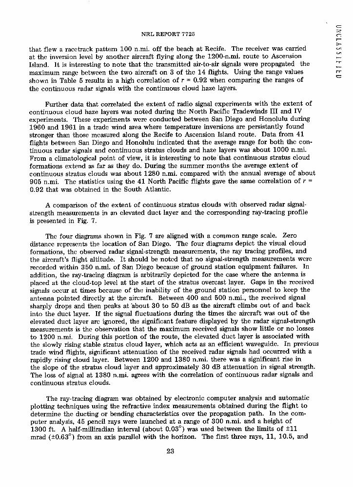
A comparison of the extent of continuous stratus clouds with observed radar signal-strength measurements in an elevated duct layer and the corresponding ray-tracing profileis presented in Fig. 7.

The four diagrams shown in Fig. 7 are aligned with a common range scale. Zerodistance represents the location of San Diego. The four diagrams depict the visual cloudformations, the observed radar signal-strength measurements, the ray tracing profiles, andthe aircraft's flight altitude. It should be noted that no signal-strength measurements wererecorded within 350 n.mi. of San Diego because of ground station equipment failures. Inaddition, the ray-tracing diagram is arbitrarily depicted for the case where the antenna isplaced at the cloud-top level at the start of the stratus overcast layer. Gaps in the receivedsignals occur at times because of the inability of the ground station personnel to keep theantenna pointed directly at the aircraft. Between 400 and 500 n.mi., the received signalsharply drops and then peaks at about 30 to 50 dB as the aircraft climbs out of and backinto the duct layer. If the signal fluctuations during the times the aircraft was out of theelevated duct layer are ignored, the significant feature displayed by the radar signal-strengthmeasurements is the observation that the maximum received signals show little or no lossesto 1200 n.mi. During this portion of the route, the elevated duct layer is associated withthe slowly rising stable stratus cloud layer, which acts as an efficient waveguide. In previoustrade wind flights, significant attenuation of the received radar signals had occurred with arapidly rising cloud layer. Between 1200 and 1380 n.mi. there was a significant rise inthe slope of the stratus cloud layer and approximately 30 dB attenuation in signal strength.The loss of signal at 1380 n.mi. agrees with the correlation of continuous radar signals andcontinuous stratus clouds.

The ray-tracing diagram was obtained by electronic computer analysis and automaticplotting techniques using the refractive index measurements obtained during the flight todetermine the ducting or bending characteristics over the propagation path. In the com-puter analysis, 45 pencil rays were launched at a range of 300 n.mi. and a height of1300 ft. A half-milliradian interval (about 0.030) was used between the limits of ±11mrad (±0.630) from an axis parallel with the horizon. The first three rays, 11, 10.5, and

23

CHARLES G. PURVES

0 200 400 600 800 1000 1200 1400 1600 1800RANGE (n.mi)

Fig. 7 -Comparison of the extent of stratus clouds with radio signal measurements andray-tracing analysis (Tradewinds IV, mission 5, February 21, 1961)

24

Ein

a£fl0-

Ia.

NRL REPORT 7725

10 mrad (+ 0.630 to + 0.570), were too steep to be trapped in the duct. The last ninerays launched between -7.0 and -11.0 mrad (-0.400 to -0.630) were also too steep to betrapped in the duct layer. The first ray trapped in the duct was launched at an angle of9.5 mrad (+0.540), and the last ray trapped in the duct layer was launched at an angle of-6.5 mrad (-0.370). Therefore, the angular spread for the 33 rays trapped in the duct was0.91°. Consequently, of the 45 rays launched, only 33 were trapped in the elevated ductlayer. If one considers the number of rays lost or escaping the duct layer as being pro-portional to the power lost, then the following mathematical relationship should exist:

total rays trapped - total rays lostthe total decibel loss = 10 log10 toa astapd. (34)

0 10 10 - total rays trapped

For the example in Fig. 7 where 33 of the 45 launched rays were trapped in theelevated duct layer, two rays escaped at 225 n.mi. from the launch point (525 n.mi. onthe range scale) and eight more rays leaked out between 300 and 250 n.mi. from thelaunch point (600 to - 650 n.mi. on the range scale). Consequently, the decibel lossfor the case of 33 trapped rays when 10 rays escaped the duct, as determined by Eq.(34), would be -1.8 dB. This loss rate shows excellent agreement with the measuredsignals for the 900 n.mi. between the 300-n.mi. launch point and the 1200-n.mi. pointwhere the stratus layer and duct interface layer immediately above the cloud tops wererising very uniformly. The resultant 30-dB peak power loss from 1200 n.mi. to 1380n.mi. is associated with the sharp rise in the slope of the stratus cloud layer and the endof the continuous stratus cloud and related elevated duct layer.

CORRELATION OF CLOUD TYPES WITH SIZE OFTEMPERATURE INVERSION

The trade wind inversion, perhaps the most important regulating valve of the generalcirculation, was first discovered in 1856 by C. Piazzi-Smyth during an astronomicalexpedition in the Canary Islands. His detailed measurements taken while climbing up anddown a mountain peak revealed a marked temperature inversion associated with a sharpdecrease in moisture content. Also noted at the time was a visual correlation betweenthe tops of the cloud layer and the temperature inversion. The first large-scale atmosphericexploration of the trade wind inversion occurred in 1926 during the 2-year GermanMeteor Expedition in the cold-water strip near the African West Coast. From numerouskite soundings taken in the North and South Atlantic trade wind areas, the Germanscientist Von Ficker [16] published what is now considered the classical treatise on tradewind inversion. Some of the more significant findings of the expedition concern theareal distribution of the heights and magnitude of the temperature inversions. Theextensive worldwide aircraft radar meteorological investigations of elevated duct layersin trade wind areas conducted by NRL between 1959 and 1962 represent a major con-tribution to knowledge of the causes and effects of trade wind inversions, about whichmuch is still to be learned.

A better understanding of radar atmospheric propagation effects caused by thetrade wind inversion is obtained by evaluating some of its significant large-scale features.From the German Meteor Expedition and NRL experiments, one of the key observationsis the relationship that exists between the height and size of the temperature inversion.These two factors have a direct relationship to visual cloud patterns and continuous

25

CHARLES G. PURVES

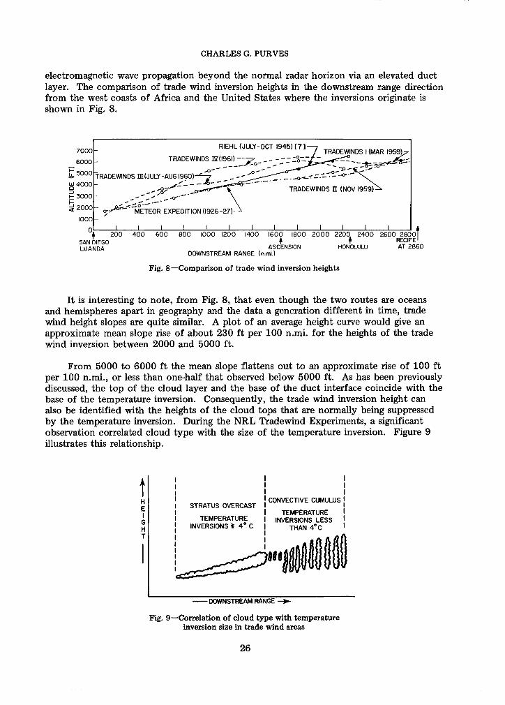
electromagnetic wave propagation beyond the normal radar horizon via an elevated ductlayer. The comparison of trade wind inversion heights in the downstream range directionfrom the west coasts of Africa and the United States where the inversions originate isshown in Fig. 8.

7000 - RIEHL (JULY-OCT 1945) [7] TRADEWINDS I (MAR 1959>

6000 _ TRADEWINDS I-961) --- _ -_0-- - _,6000 -~ ~~~~-- o

L 5000 TRADEWINDS M (JULY -AUG 1960)_7_ _-UJ 4000 --- ~ f

4 3000 o-' - 8 - _ TRADEWINDS H (NOV 1959)

2000< 2000 -;>b METEOR EXPEDITION (1926-27)1000 _

o I l l I l l I I I I I I I i* 200 400 600 800 1000 1200 1400 1600 1800 2000 2200 2400 2600 2800

SAN DIEGO * RECIFELUANDA ASCENSION HONOLULU AT 2860

DOWNSTREAM RANGE (n.mi.)

Fig. 8-Comparison of trade wind inversion heights

It is interesting to note, from Fig. 8, that even though the two routes are oceansand hemispheres apart in geography and the data a generation different in time, tradewind height slopes are quite similar. A plot of an average height curve would give anapproximate mean slope rise of about 230 ft per 100 n.mi. for the heights of the tradewind inversion between 2000 and 5000 ft.

From 5000 to 6000 ft the mean slope flattens out to an approximate rise of 100 ftper 100 n.mi., or less than one-half that observed below 5000 ft. As has been previouslydiscussed, the top of the cloud layer and the base of the duct interface coincide with thebase of the temperature inversion. Consequently, the trade wind inversion height canalso be identified with the heights of the cloud tops that are normally being suppressedby the temperature inversion. During the NRL Tradewind Experiments, a significantobservation correlated cloud type with the size of the temperature inversion. Figure 9illustrates this relationship.

tH | CONVECTIVE CUMULUS IE I STRATUS OVERCAST I. I|I TEMPERATURE IG I TEMPERATURE I INVERSIONS LESS IH INVERSIONS 2 4° C I THAN 40CT I

DOWNSTREAM RANGE --

Fig. 9-Correlation of cloud type with temperatureinversion size in trade wind areas

26

NRL REPORT 7725

The last 10 flights of the Tradewinds IV San Diego to Honolulu route were carefullyexamined to determine the validity of the critical temperature inversion relationship tocloud type as depicted in Fig. 9. To remove ambiguity, only soundings or probes thatwent 1000 ft above the cloud tops were evaluated because during straight and level flightit is not possible to determine the full value of the temperature inversion size.

Out of 53 cases, 49 showed agreement with the critical 40 C temperature inversion-cloud type correlation. Three of the four cases that did not conform were within 400 miof the California coast where the cloud tops were less than 2000 ft. These cases can belinked to large-scale meteorological conditions that create exceptions to the generalcorrelation between cloud type and size of temperature inversion.

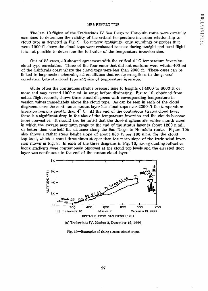
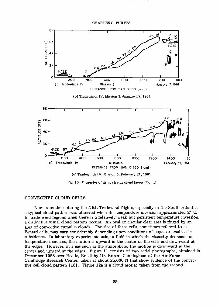
Quite often the continuous stratus overcast rises to heights of 4000 to 6000 ft ormore and may exceed 1000 n.mi. in range before dissipating. Figure 10, obtained fromactual flight records, shows three cloud diagrams with corresponding temperature in-version values immediately above the cloud tops. As can be seen in each of the clouddiagrams, once the continuous stratus layer has cloud tops over 2000 ft the temperatureinversion remains greater than 40 C. At the end of the continuous stratus cloud layerthere is a significant drop in the size of the temperature inversion and the clouds becomemore convective. It should also be noted that the three diagrams are winter month casesin which the average maximum range to the end of the stratus layer is about 1200 n.mi.,or better than one-half the distance along the San Diego to Honolulu route. Figure 10balso shows a rather steep height slope of about 833 ft per 100 n.mi. for the cloudtop level, which is about three times steeper than the mean slope of the trade wind inver-sion shown in Fig. 8. In each of the three diagrams in Fig. 10, strong ducting refractiveindex gradients were continuously observed at the cloud top levels and the elevated ductlayer was continuous to the end of the stratus cloud layer.

8K _ I I

0.8

wL 66 3 0

4K

I-2K

HAZE 88 104'

0-200 400 600 800 1000 1200

(a) Tradewinds IV Mission 2 December 19, 1960

DISTANCE FROM SAN DIEGO (n.mi)

(a) Tradewinds IV, Mission 2, December 19, 1960

Fig. 10-Examples of rising stratus cloud layers

27

CHARLES G. PURVES

8K

200(b) Tradewinds IV

400 600Mission 3

DISTANCE FROM

800

SAN DIEGO (n.mi)

(b) Tradewinds IV, Mission 3, January 17, 1961

0

I-

-j

200 400 600 800 1000 1200 1400 16((c) Tradewinds IV Mission 5 February 21,1961

DISTANCE FROM SAN DIEGO (n.mi.)

(c) Tradewinds IV, Mission 5, February 21, 1961

Fig. 10-Examples of rising stratus cloud layers (Cont.)

CONVECTIVE CLOUD CELLS

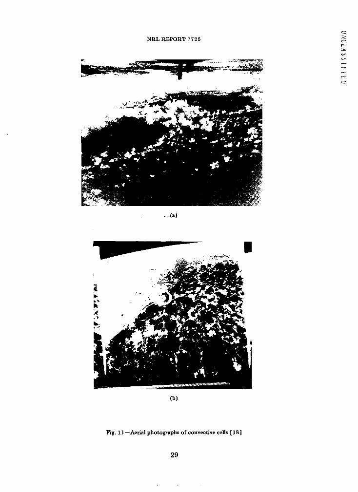
Numerous times during the NRL Tradewind flights, especially in the South Atlantic,a typical cloud pattern was observed when the temperature inversion approximated 20 C.In trade wind regions when there is a relatively weak but persistent temperature inversion,a distinctive visual cloud pattern occurs. An oval or circular clear area is ringed by anarea of convective cumulus clouds. The size of these cells, sometimes referred to asBenard cells, may vary considerably depending upon conditions of large- or small-scalesubsidence. In laboratory experiments using a fluid in which the viscosity decreases astemperature increases, the motion is upward in the center of the cells and downward atthe edges. However, in a gas such as the atmosphere, the motion is downward in thecenter and upward at the edges. Figure 11 consists of two aerial photographs, obtained inDecember 1958 over Recife, Brazil by Dr. Robert Cunningham of the Air ForceCambridge Research Center, taken at about 25,000 ft that show evidence of the convec-tive cell cloud pattern [18]. Figure 12a is a cloud mosiac taken from the second

28

0I-

I-

6K

4K

2K

-I?, ~~~0

2.5 910.4 amp#

HAZE 7/ HZI e"l I I I I0

1000 1200 1400January 17, 1961

NRL REPORT 7725

or. PT;w x~l~~~~~~~~~~~~~~~~~~~~~~~~ -1

. (a)

I

(b)

Fig. 11-Aerial photographs of convective cells [18]

29

r-.* _v - - :- .-

CHARLES G. PURVES

) 20 40 60 80(b) DISTANCE (n.mi.)

20 40 60 80DISTANCE (n.mi.)

7tD W(a) Cloud mosaic from second54 photograph in Fig. 11

I

,(b) Path A-route of minimum cloudiness

(c) Path B-route of maximum cloudiness

100 120

Fig. 12-Routes of minimum and maximum cloudiness in convective cell areas [18]

30

8000

6000ILU-

0D 4000I--

2000

8000 r-

6000 H

4000 I0I-,

2000

LIzb ttlttltll~tt, " I 00 CLEAR

3 5 7 4 3 5 7 4 < 2 410 10 1I I1 0 10 10 10

I I I I IU ).0

(c)

A\

NRL REPORT 7725

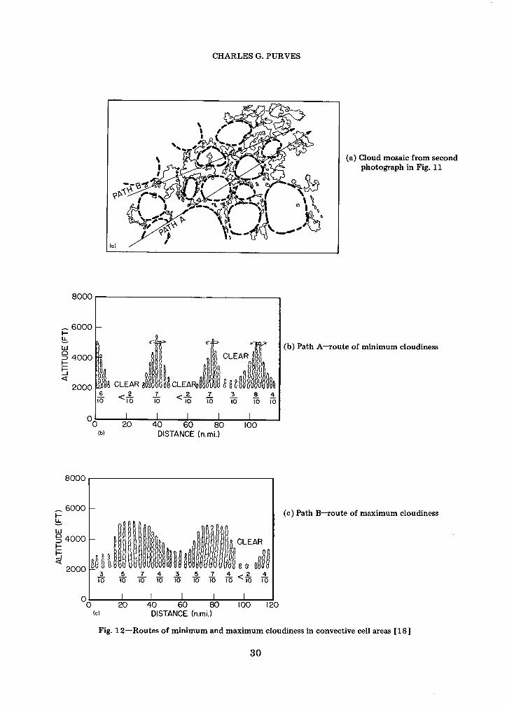
photograph in Fig. 11. Figures 12b and 12c illustrate the significant differences in cloudstructure that exist along two adjacent paths [18]. Figures 11 and 12 illustrate thesignificant characteristics of convective cell clouds as related to electromagnetic wavepropagation.

In Fig. 12, path A represents a route of minimum cloudiness and path B a route ofmaximum cloudiness close to path A. A typical cloud diagram depicting these two pathsis shown in Figs. 12b and 12c. The ranges indicated on the cloud cross-section diagramsare based on visual observations and are considered to be representative. The areas ofmaximum cloudiness are related to areas of convergence resulting in vertical updraftmotions. The clear areas are the result of subsidence and divergence and are related tosinking air from aloft, which causes the air to be warmer and drier than the surroundingair. Frequently these clear cells extend down to the sea surface, and it is interestingto note that the cloud heights are visually related to the inverted bulges, or clear cells, thatpermeate the area. When flying at low altitudes, it is very difficult to recognize theseconvective cells, as they must be seen from a high vantage point to be recognized as such.Compared to the continuous stratus cloud layers, propagation conditions through areaswhere convective cells commonly occur cannot be statistically documented in terms ofthe predicability of continuous propagation. However, the overall high frequencies ofcontinuous and intermittent long stretches of received air-to-air radar signals observedover the Recife to Ascension Island route were many times propagated through large-scale areas of convective cells. In all probability it is reasonable to assume that betterpropagation conditions would result in a route of minimum cloudiness because a morecloudy route, such as path B in Fig. 12a, is subject to more unstable air, which becauseof increased vertical development is dissipating the intensity of the temperature inversion.

RAY TRACING USED TO EVALUATE ANOMALOUSRADAR PROPAGATION EFFECTS

There is little question that the state of the art in providing RIF's will be greatlyenhanced by the use of digital and analog computers. Additional research is needed toprovide adequately acceptable atmospheric models to improve the Navy's forecastcapabilities. A graphic display of a family of rays emanating from a radar transmitter,showing the behavior of each pencil ray as it travels through space, certainly gives theoperational analyst a more realistic picture of the causes and effects associated withanomalous radar propagation. Simple usable models have existed for over a generationthat show very complex cross-sectional diagrams when using refractive index profilesobtained in nonstandard atmospheric conditions. With the advent of satellite photography,the meteorologists and cloud physicists are gaining a much better understanding of therelationship between basic cloud types and synoptic weather conditions. The use of thecomputer allows both the hypothetical and actual complex measured cases to beevaluated. Many aspects of radar propagation, such as ducting, radar holes, antiholes,irregularities in signal fluctuation, range and elevation angle errors, and the effects causedby the changing height of a radar transmitter are more readily evaluated by electroniccomputers.

During the NRL Pacific Tradewinds flights, there were cases in which a continuousstratus layer in the downstream direction would have gradual, steady, evenly rising slopes,

31

CHARLES G. PURVES

sudden abrupt increases in slope rates, no rise in cioud-top levels, and a decrease in cloud-top levels. As previously discussed, the more typical case was slowly rising cloud height,with a gradual increase in the downstream direction. The sudden abrupt increases in thecloud-top level were often associated with cases of either small- or large-scale convergence,such as those experienced when the strength of the temperature inversion weakened toless than 40 C and convective cumulus clouds pushed upward because of increased verticalmotion as the trade wind inversion weakened. Another meteorological factor related to asharp rise in cloud tops was associated with a high-pressure ridge. A leveling of the cloudtops was usually an indication of increasing subsidence, which would normally result inan increase in the size of the temperature inversion. The times that the cloud heightswere decreasing in the downstream direction were usually when the stratus cloud tops werebelow 2000 ft, very thin in depth, and within a few hundred miles of the Californiacoast. Usually in these instances the size of the temperature inversion was quite large,perhaps in excess of 100 C, and multiple haze layers were present above the cloud tops.

Several years after the NRL Pacific Tradewinds propagation experiments, an NRLReport 6253 [19] was published that showed ray-tracing examples for cases of risingand falling duct layers. The mathematic model used for the computer plots of the ray-tracing examples is fully explained in the report. Figures 13 to 16, published in Ref. 19as Fig. 8 to 11, are presented to illustrate the value of using ray-tracing profiles inareas where anomalous radar propagation effects are associated with elevated duct layers.

SATELLITE CLOUD PHOTOGRAPHY USED FORREFRACTIVE INDEX FORECASTING

French scientists Schereschewsky and Wehrle are noted for their analysis of weatherbased solely on cloud observations [20]. They developed a mapping of cloud systems inFrance as early as 1923. A correlation of visual cloud observations with frontal synopticweather conditions, especially in areas where standard weather stations are very sparcesuch as in Africa, was successfully used as a supplemental forecasting technique. In morerecent times a number of meteorologists have used correlation methods involving cloudpatterns to explain large-scale synoptic weather. Today's professional forecasters arefinding more ways of utilizing cloud information in local and large-scale weather fore-casting.

The NRL Tradewinds experiments clearly indicate that a correlation exists betweencloud types, temperature inversion magnitude, and propagation conditions via an elevatedduct layer. Additional research of this type in other than trade-wind areas is needed tohave a better understanding of this subject.

In the past, the visual observing of cloud information normally recorded on synopticweather charts was far from ideal. However, the gross cloud picture could usually beidentified with large synoptic weather patterns. The current weather satellite programoffers a new observation technique capable of giving worldwide synoptic coverage ofweather conditions. The continuing use of satellite cloud photography is resulting inmore reliable and detailed cloud charts, which are helping to improve the state of the artin local weather forecasts. Satellite cloud photographs already give evidence of morelarge-scale organization of cloud patterns than previously had been conceived. Theorientation of frontal bands, cyclonic swirls, and other organized patterns is so pronounced

32

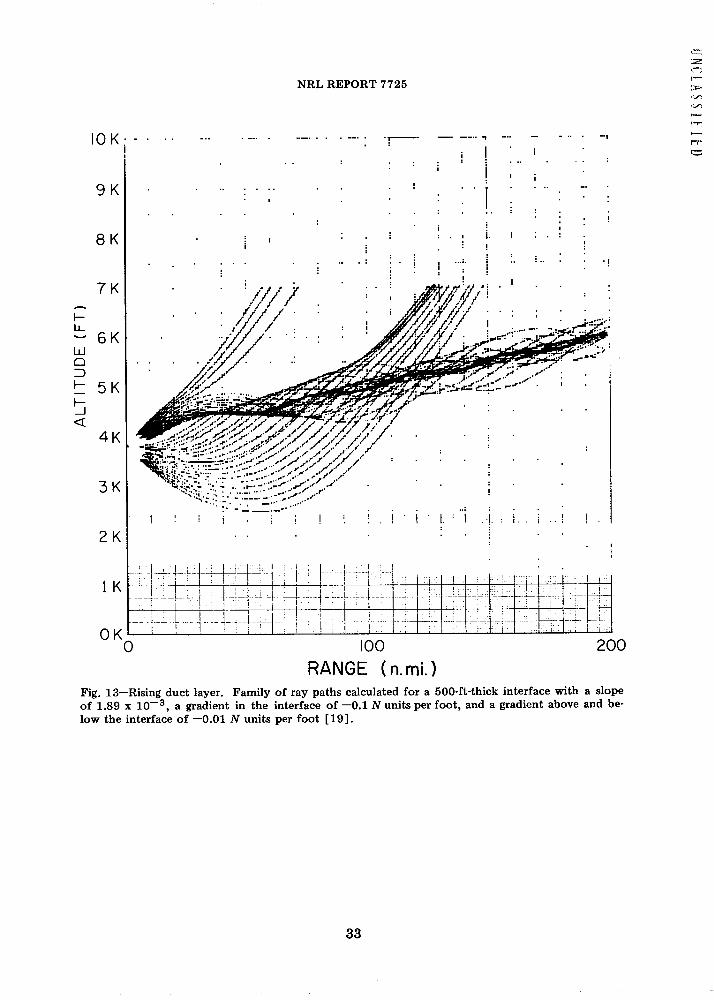
NRL REPORT 7725

10K

9 K

8 K

7 K

6 K

5 K

4K

3 K

2 K

1 K

0 K0

' IL 1I 1_ ' - ]. -A- rL -__! I-I :111 ___

-t �-TTA?-�V 1 <� -

100 200RANGE (n.mi.)

Fig. 13-Rising duct layer. Family of ray paths calculated for a 500-ft-thick interface with a slopeof 1.89 x 10-3, a gradient in the interface of -0.1 N units per foot, and a gradient above and be-low the interface of -0.01 N units per foot [19].

33

LL

UJ

D

I-

iI

A_

I

S i

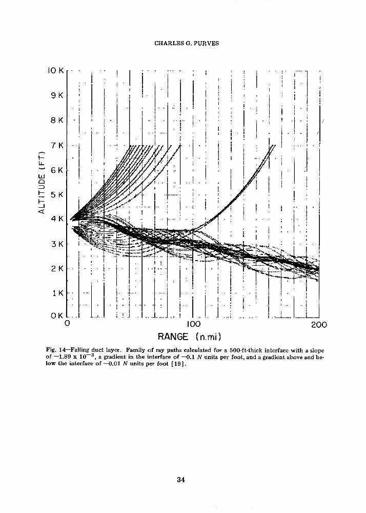
CHARLES G. PURVES

10K .

9K

8K

7K ..i .

- 6KILI

<4 K .4

a

3LK

2K ..

-J -

OK ..0

1%,I 'AK/1

II

* . ~~~. ....* I

. .I

*: ' i

: !F~~~.

I* *

100

RANGE (n.mi)Fig. 14-Falling duct layer. Family of ray paths calculated for a 500-ft-thick interface with a slopeof -1.89 x 10-3, a gradient in the interface of -0.1 N units per foot, and a gradient above and be-low the interface of -0.01 N units per foot [19].

34

/

200

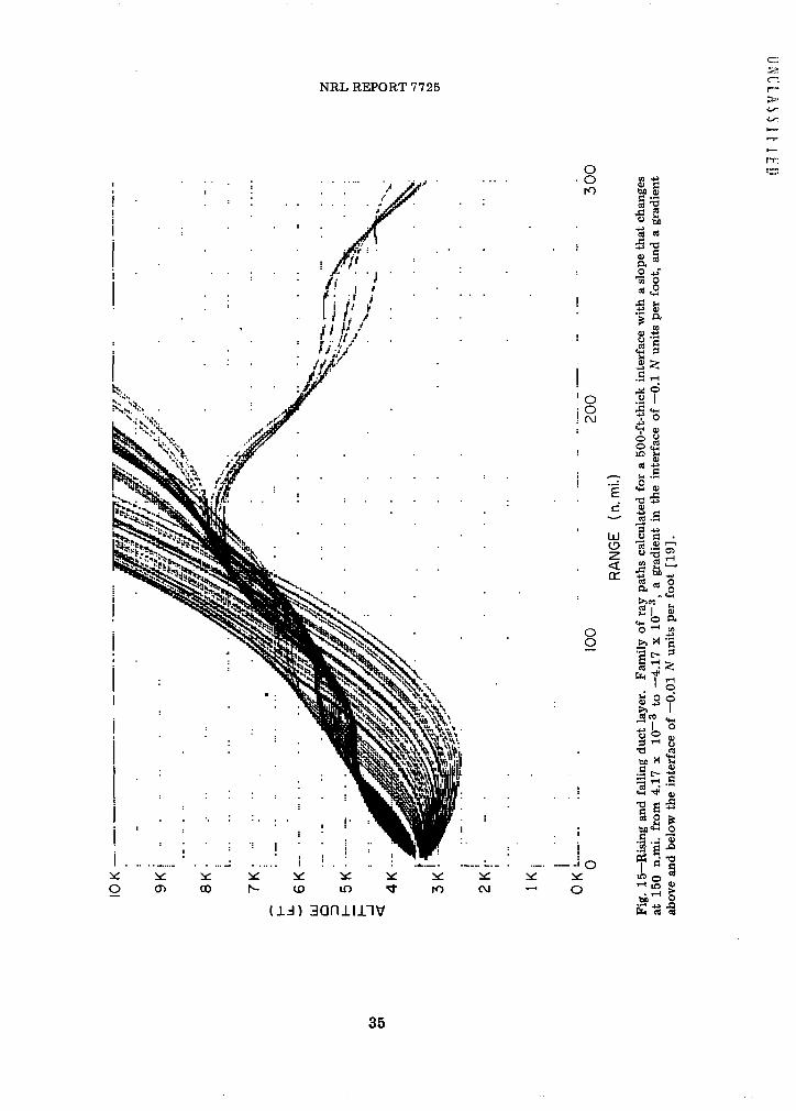
II .

I . . ..

i ..... . . ... .. ...Y Y Y Y Yo u) OD) N- 3L

(IA) I

NRL REPORT 7725

rr0

* o3 cCd

/1' ~ ~ ~ ~ ~ 1

'0Cjooj y/. .... ..! 8 -~~~~~~. 4

tos

4) Q (I °~

~K. 8

CZ

0 _

2~~~~~~z~~~~~~~ r b

;) 'V ;o 0. - C)'ortn liL OV

3anlllnu N Y n~~~~~~~~~~~~~~~~~~~~~T

35

i

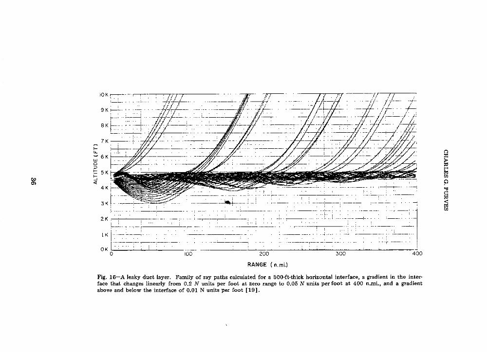
9 K - 77 *X A- l

.. . . . ........ .- ..

9 K j -- -----------...--__... ___

O K I . . . . - ' - '--- - -- - - - - - .. - .. _ . .

6 K~~~~~~~~~~~~~~~~~~~~~~~~~~~~~~~~~~~~~~~~~~~

O . 0 200 300.40

5 KrCAD /

4KC~

2 K

OKL . ...... _________________

0 100~~b - 200 300 400

RANGE (n. mi.)

Fig. 16-A leaky duct layer. Family of ray paths calculated for a 500-ft-thick horizontal interface, a gradient in the inter-face that changes linearly from 0.2 N units per foot at zero range to 0.05 N units per foot at 400 n.mi., and a gradientabove and below the interface of 0.01 N units per foot [19].

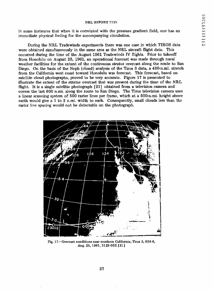
NRL REPORT 7725

in some instances that when it is correlated with the pressure gradient field, one has animmediate physical feeling for the accompanying circulation.

During the NRL Tradewinds experiments there was one case in which TIROS datawere obtained simultaneously in the same area as the NRL aircraft flight data. Thisoccurred during the time of the August 1961 Tradewinds IV flights. Prior to takeofffrom Honolulu on August 25, 1961, an operational forecast was made through navalweather facilities for the extent of the continuous stratus overcast along the route to SanDiego. On the basis of the Neph (cloud) analysis of the Tiros 3 data, a 400-n.mi. stretchfrom the California west coast toward Honolulu was forecast. This forecast, based onsatellite cloud photographs, proved to be very accurate. Figure 17 is presented toillustrate the extent of the stratus overcast that was present during the time of the NRLflight. It is a single satellite photograph [21] obtained from a television camera andcovers the last 600 n.mi. along the route to San Diego. The Tiros television camera usesa linear scanning system of 500 raster lines per frame, which at a 500-n.mi. height aboveearth would give a 1 to 3 n.mi. width to each. Consequently, small clouds less than theraster line spacing would not be detectable on the photograph.

iI

I

I

Fig. 17-Overcast conditions near southern California; Tiros 3, 638-8,Aug. 25, 1961, 2123-05Z [21]

37

CHARLES G. PURVES

A cloud mosiac showing the areas covered by clouds on both sides of the aircrafttrack for over one-half the route is presented in Fig. 18. The cloud mosaic is madefrom a compilation of individual satellite cloud photographs. Hourly positions of theaircraft are shown for the last 7 hr of flight. A confident prediction of a continuouselevated duct for any of the continuous stratus overcast areas shown in the cloud mosaicfrom the California coast to approximately 1250 W longitude can be made on the basisof previously observed radar signal measurements over this route. The use of similarsatellite cloud photographs is a definite aid in predicting large-scale propagation conditions.

THE STATE OF THE ART IN MAKING AREFRACTIVE INDEX FORECAST

The ability to make an accurate real-time RIF for specific oceanic regions on aglobal basis is of special concern to naval operations. At best this service is very limitedor nonexistent. To make reliable forecasts it is necessary to have a network of observingstations that can measure refractive indexes accurately. It is also essential to have astockpile of climatological records that would give local geographic summaries of what isstatistically expected in terms of refractive index profiles. Having such information wouldgive fleet commanders and other naval operational personnel a better background knowledgeof what to expect in strategic areas on a monthly or seasonal basis. Present-day globalsynoptic meteorological and oceanographic forecasting services are enhanced by theutilization of computerized forecasting techniques. Short-range forecasts (less than a day)and long-range surface and upper-air forecasts of 5 days or more are routinely suppliedfor almost any geographic region in the world. Where atmospheric forecasts are needed,the prime source of measuring the significant meteorological parameters of pressure,temperature, and humidity for the past generation comes from an international globalnetwork of weather stations that makes use of atmospheric profiles obtained from ascend-ing balloonborne radiosonde measurements.

The radiosonde is a slow-response instrument that measures temperature, pressure,and moisture content of the air while being carried aloft by a lighter-than-air balloon,which eventually bursts, often above 100,000 ft. Most computer forecasts using radiosondedata make use of smoothing, or averaging, techniques that do not require fast-response-timeinstruments to get desired forecast results. A RIF, however, requires both accurate andfast-response measuring instruments, especially for the vapor pressure and temperatureparameters. Consequently, the use of radiosonde data seriously limits the ability to detectaccurately the significant refractive index gradients needed to obtain a reliable RIF. Cur-rently, the best instrument for obtaining an atmospheric profile of refractive indexes is anairborne microwave refractometer, which has been used only sparsely since the 1950's,mainly by research and reconnaissance type aircraft.

RECOMMENDATIONS

Action should be initiated to establish a central depositor for the collection andfiling, in a computerized system, of all refractive index profile measurements obtained bymicrowave refractometers and to require all commands to forward routinely all such datato the designated record center within a reasonable time. In this manner a stockpile ofreference material would be available eventually for statistical summary and use by those

38

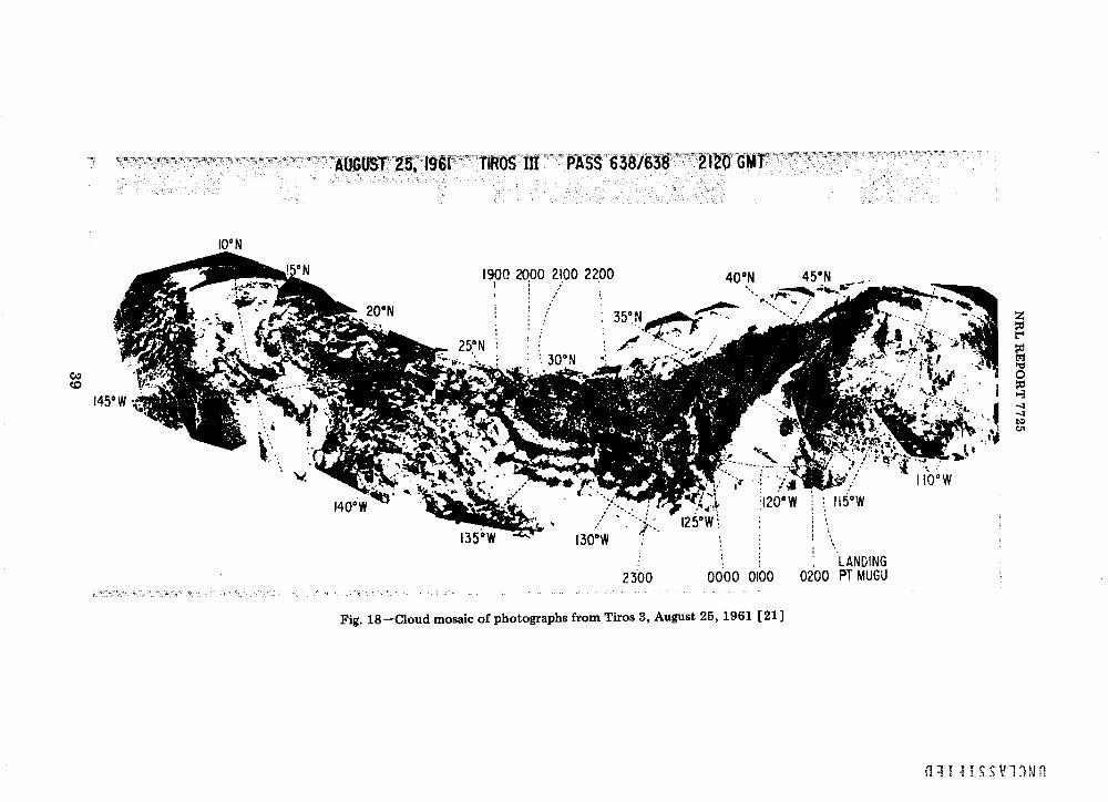
AU'<S' 25, 19' 1 tIROS m At 6 /63P i:GT;

10 N

20°N

1900

_ 250 N:

2000 2100 2200 40°N 45°N30° x 1- .

; : .350 N -

. * -

: 00,N Ar--."

140 0W

. .130OW 'I

2300 0000 0100

Fig. 18-Cloud mosaic of photographs from Tiros 3, August 25, 1961 [21]

-,., ,. -:-

Y. '. 115°W

LANDING0200 PT MUGU

_i J. i M I f lyni

CoCd

!45° W

I

i z1 kx * ds .:]

-- -..- ,. 4

J i- -I. I ..

.120° W, .4- A,

. .!v

I 10OW

.W.�

I -.4J.

-i

*t. ;- .

i

CHARLES G. PURVES

having a need for such data. In this respect, it would also be advisable for the Navy,where possible, to collect all known past microwave refractometer records because thecost to resurrect and use this type of data would be nominal when compared to the costof obtaining similar records by performing new flights in the areas where the data werefirst observed.

A computerized ray-tracing capability should be developed by means of which a shipcommander could obtain the best available forecast in the area of concern by making useof on-the-spot data to generate a two-dimensional computerized family of ray paths thatwould best describe the presence of anomalous propagation conditions.

Other methods should be developed, such as satellite cloud photography, that wouldallow cloud correlation techniques to give a secondary forecast capability on a global real-time basis from existing forecast centers via Teletype or satellite communication iinks.

More atmospheric model cases should be developed that could possibly be used inconjunction with satellite cloud coverage photography, large-scale synoptic weather patterns,weather reconnaissance data, or any other significant weather relationship that can becorrelated to give a RIF.

A reference atlas of ray-tracing profiles should be compiled that could be used tocharacterize, or correlate, typical past weather conditions with present synoptic weather.

A committee of naval civilian and military scientists experienced in the field ofelectromagnetic wave propagation should be established to review and update the presentknowledge of anomalous propagation so that this information can be more advantageouslyused to improve the state of the art of making a RIF.

New research programs that would enhance the state of the art of making a RIF,should be initiated.

REFERENCES

1. H.G. Booker, "Some Problems in Radio Meteorology," Quart. J. Roy. Meteorol. Soc.74, 277-307 (1948).

2. D.R. Jones, "Meteorological Refractive Effects Upon Radar Wave Propagation,"NAVAER 50-1 P-527, July 1, 1954, p. 8; prepared at Project AROWA, U.S. FleetWeather Control, Norfolk, Va.

3. D.E. Kerr, editor, Propagation of Short Radio Waves, Dover Publications, Inc., NewYork, 1965, p. 21.

4. M.I. Skolnik, Introduction to Radar Systems, McGraw-Hill, New York, 1962, p. 8.

5. W.F. Freiberger, editor, International Dictionary of Applied Mathematics, VanNostrand, Princeton, N.J., 1960, pp. 851-852.

6. E.K. Smith, Jr., and S. Weintraub, "The Constants in the Equation for AtmosphericRefractive Index at Radio Frequencies," Proc. IRE 41, No. 8, 1035-1037 (Aug.1953).

40

NRL REPORT 7725

7. F.A. Berry, Jr., E. Bollay, and N.R. Beers, editors, Handbook of Meteorology,McGraw-Hill, New York, 1945, p. 373.

8. L.B. Battan, Radar Meteorology, 2d impression, The University of Chicago Press,Chicago, 1960, p. 18.

9. CRC Standard Mathematical Tables, 10th ed., Chemical Rubber Publishing Co.,Cleveland, 1954, p. 15.

10. NWRF 31-0660-035, "Meteorological Aspects of Radio-Radar Propagation," U.S.Navy Weather Research Facility, Norfolk, Va., 1960, pp. 46-69.

11. B.R. Bean, B.A. Cahoon, C.A. Sampson, and G.D. Thayer, A World Atlas of Atmos-pheric Radio Refractivity, U.S. Department of Commerce Environmental ScienceServices Administration, U.S. Government Printing Office, Washington, D.C., 1966.

12. H.L. Crutcher and O.M. Davis, "U.S. Navy Marine Climatic Atlas of the World,"Volume VIII in The World, NAVAIR 50-1C-54, Mar. 1, 1969.

13. C.G. Purves, "'Synopsis of December 1960 Flight of Project Tradewinds IV," NRLLtr. Rept. 5270-32, NRL Problem R07-05, Aug. 23, 1961.

14. C.G. Purves, "Synopsis of February 1961 Flight of Project Tradewinds IV," NRL Ltr.Rept. 5270-34, NRL Problem R07-05, Aug. 23, 1961.

15. Wave Propagation Branch Rept. "220-Mc Propagation in an Elevated Duct," Reportof NRL Progress, Washignton, D.C., May 1960, pp. 1-15.

16. H. Ficker, Ver6ff. Meteor. Inst. Berlin I, No. 4 (1936).

17. H. Riehl, Tropical Meteorology, McGraw-Hill, New York, 1954, pp 63, 65-66.

18. C.G. Purves, "Meteorological Aspects of Radio Propagation in Tradewind Areas," inProceedings of the Fifth Navy Science Symposium, ONR-9, Vol. 3, pp. 812-822,Office of Naval Research, Washington, D.C., 1961.

19. N.W. Guinard, M.B. Laing, and K. Morin, "Ray Tracing in Rising and Falling Ducts,"NRL Rept. 6253, June 22, 1965.

20. P.L. Shereschewsky and P. Wehrle, "Les Systems Nuageau," Off. Nat. Meteor. Memo.No. 1, Paris, 1923.

21. C.G. Purves, "A Month-by-Month Study of the Elevated Duct Between San Diego andHawaii," NRL Memorandum Report 1416, Apr. 3, 1963.

41