Embed Size (px)
Citation preview

Advances in Engineering Software xxx (2011) xxx–xxx
Contents lists available at ScienceDirect
Advances in Engineering Software
journal homepage: www.elsevier .com/locate /advengsoft
GeoPDEs: A research tool for Isogeometric Analysis of PDEs
C. de Falco a,⇑, A. Reali b,c,d, R. Vázquez c
a MOX-Modeling and Scientific Computing, Dipartimento di Matematica, Politecnico di Milano, Piazza Leonardo da Vinci, 32, 20133 Milano, Italyb Dipartimento di Meccanica Strutturale, Università degli Studi di Pavia, Via Ferrata, 1, 27100 Pavia, Italyc Istituto di Matematica Applicata e Tecnologie Informatiche del CNR, Via Ferrata, 1, 27100 Pavia, Italyd EUCENTRE, via Ferrata, 1, 27100 Pavia, Italy
a r t i c l e i n f o
Article history:Received 27 October 2010Received in revised form 5 May 2011Accepted 22 June 2011Available online xxxx
Keywords:Isogeometric AnalysisFinite element methodNURBSB-SplinesMatlabOctave
0965-9978/$ - see front matter � 2011 Elsevier Ltd. Adoi:10.1016/j.advengsoft.2011.06.010
⇑ Corresponding author.E-mail addresses: [email protected] (C. de Fal
(A. Reali), [email protected] (R. Vázquez).
Please cite this article in press as: de Falco Cj.advengsoft.2011.06.010
a b s t r a c t
GeoPDEs (http://geopdes.sourceforge.net) is a suite of free software tools for applications on Isogeomet-ric Analysis (IGA). Its main focus is on providing a common framework for the implementation of themany IGA methods for the discretization of partial differential equations currently studied, mainly basedon B-Splines and Non-Uniform Rational B-Splines (NURBS), while being flexible enough to allow users toimplement new and more general methods with a relatively small effort. This paper presents the philos-ophy at the basis of the design of GeoPDEs and its relation to a quite comprehensive, abstract definitionof IGA.
� 2011 Elsevier Ltd. All rights reserved.
1. Introduction
Isogeometric Analysis (IGA) is a (relatively) recent technique forthe discretization of Partial Differential Equations (PDEs), intro-duced by Hughes et al. in [1]. The main feature of the method isthe ability to maintain the same exact description of the computa-tional domain geometry throughout the analysis process, includingrefinement. In the original presentation of IGA as described in [1](where one of the main focuses is on structural analysis), the exactgeometry representation is obtained by invoking the isoparametricconcept, that is, by using the same class of functions most com-monly used for geometry parameterization in Computer AidedGeometric Design (CAGD), namely Non-Uniform Rational B-Splines(NURBS), for the PDE solution space. As NURBS spaces include as aspecial case the piece-wise polynomial spaces commonly used inthe Finite Element Method (FEM), IGA can be understood as a gen-eralization of standard FEMs where more regular functions are em-ployed. This higher regularity has been shown to lead to variousadvantages of IGA over FEM in addition to the better handling ofCAGD geometries, e.g., better convergence on a per-degree-of-freedom basis, better approximation of the the eigenspectrum of
ll rights reserved.
co), [email protected]
et al. GeoPDEs: A research too
the Laplacian and biharmonic operators [2] or the ability to dealwith higher order differential operators [3,4].
Since its introduction, IGA has evolved along different direc-tions. On one hand, function spaces other than NURBS or B-Splineshave been considered, such as T-Splines [5,6], which allow for localrefinement, or so-called generalized B-Splines [7,8], that allow tobetter handle important classes of curves and surfaces. On theother hand, especially for applications where the propertiesdescending from a strictly isoparametric approach are not of suchparamount importance as for structural analysis, the isoparametricconstraint has been relaxed in order to produce B-Spline general-izations of edge and face finite elements [9] which have been suc-cessfully applied to problems in electromagnetism [9,10] andincompressible fluid dynamics [11]. A comprehensive referenceon IGA advantages and successful applications is the recent bookby Cottrell et al. [12].
IGA is indeed a powerful method, which has been shown to out-perform FEM in every numerical test we have tried so far. The largenumber of papers, presentations and dedicated symposia at inter-national conferences on the topic clearly indicate the great interestthat IGA has has been drawing from the PDE discretization andCAGD research communities. Nonetheless, researchers from bothsuch areas often refrain from getting directly involved in IGA be-cause of their reluctance to invest the time and effort required toget acquainted with the basics of each other’s field. Furthermore,for those working on complex engineering applications, theamount of work required to adapt their existing codes to the IGA
l for Isogeometric Analysis of PDEs. Adv Eng Softw (2011), doi:10.1016/
2 C. de Falco et al. / Advances in Engineering Software xxx (2011) xxx–xxx
framework would need to be carefully estimated before undertak-ing such a task.1
Bearing in mind the above-mentioned considerations, we havedecided to implement and distribute the GeoPDEs software suite[15] with multiple objectives. First, it is meant to serve as an entrypoint for researchers who wish to get acquainted with the practicalissues that implementing an IGA code involves. Furthermore, bydecoupling as much as possible the various aspects of IGA-relatedalgorithms (e.g., basis function definition and evaluation, differen-tial operator discretization, choice of function spaces, numericalquadrature, etc.), it intends to allow the users mainly interestedin one of such aspects to test their ideas in a complete solver envi-ronment while having to deal as little as possible with issues thatfall outside their area of expertise. Finally, it is meant to be used asa rapid prototyping and testing tool for new IGA algorithms.
The design of the GeoPDEs suite descends directly from theobjectives stated above, in particular the decision to implementit as an open and free software platform is driven by the intentionto use it as a way to communicate and share ideas related to IGAamong researchers from different areas; similarly, to allow itsuse as a fast prototyping tool, it has been implemented mainly inan interpreted language, the particular language of choice beingMatlab which is a de facto standard for prototyping of numericalalgorithms. Finally, to maximize its accessibility and availability,GeoPDEs has been especially optimized to work in the free GNU/Octave interpreter [16].
The present paper is not expected to be a full user guide toGeoPDEs. Rather, it is intended to explain its architecture, its de-sign and its main features, and to provide various examples ofhow to use and extend it. Furthermore, as in the implementationof GeoPDEs, given its design objectives, properties such as codeclarity, generality and extensibility have been often favored overefficiency and scalability, we will, at times, explain how some ofthe current speed or memory bottlenecks may be avoided.
The paper is structured as follows. In Section 2 we present anoverview on IGA, and in Section 3 we focus on its application tothe particular case of Poisson’s problem. The backbone of the codeis presented in Section 4, with a detailed description of its maindata structures and the help of a simple example. The way to mod-ify the code for developing new methods is explained in Section 5,and in particular we show modified versions to solve linear elastic-ity, Stokes, and Maxwell’s equations. Finally, in Section 6 we showthe extension of the code to problems on NURBS multipatchgeometries.
2. A brief overview on Isogeometric Analysis
As stated in the introduction, the initial concept of IGA has beenextended and generalized in many ways. In this paper, we intendto demonstrate the ability of GeoPDEs to accommodate withinits framework various different IGA formulations. To this end, wefind it convenient to briefly present, in the next section, the mainconcepts of IGA in a general framework. To introduce some usefulnotation, we will as well introduce, in Section 2.2 NURBS and B-Splines, which have been the first and simplest (and, so far, mostsuccessful) functions adopted in IGA.
2.1. Isogeometric Analysis: a general framework
The goal of IGA, as it is also for FEM, is the numerical approxi-mation of the solution of PDEs. In both approaches the PDEs arenumerically solved using a Galerkin procedure, i.e., the equations
1 Techniques meant to ease the adaptation of existing FEM software to the IGAsetting have been presented in [13,14].
Please cite this article in press as: de Falco C et al. GeoPDEs: A research tooj.advengsoft.2011.06.010
are written in their equivalent variational formulations, and a solu-tion is sought in a finite dimensional space with good approxima-tion properties. The main difference between the twomethodologies is that in FEM the basis functions and the computa-tional geometry (i.e., the mesh) are defined using piecewise poly-nomials, whereas in IGA the computational geometry is definedexactly from the information and the basis functions (e.g., NURBS,T-Splines, or generalized B-Splines) given by CAD.
Let us consider a three-dimensional case, where we assume thatthe physical domain X � R3 is open, bounded and Lipschitz. Wealso assume that such a domain can be exactly described througha parameterization of the form
F : bX ! X; ð1Þ
where bX is some parametric domain (e.g., the unit cube), and thevalue of the parameterization can be computed with the informa-tion given by the CAD software. The parameterization F is assumedto be smooth with piecewise smooth inverse.
Now, let V be a Hilbert space of functions defined in X, and let V0
be its dual. We denote by (�, �) the scalar product in V, and by h�, �ithe duality pairing between V0 and V. We study now the followingsource and eigenvalue problems. Given the bilinear forma : V � V ! R and the linear functional l 2 V0, the variational for-mulation of the source problem reads:
Find u 2 V such that
aðu;vÞ ¼ hl;vi 8v 2 V ; ð2Þ
whereas the variational formulation of the eigenvalue problem is:Find k 2 R n f0g, and u 2 V, u – 0, such that
aðu;vÞ ¼ kðu;vÞ 8v 2 V : ð3Þ
The Galerkin procedure, then, consists of approximating the infi-nite-dimensional space V by a finite-dimensional space Vh, and tosolve the corresponding discrete source problem:
Find uh 2 Vh such that
aðuh;vhÞ ¼ hl;vhi 8vh 2 Vh; ð4Þ
or discrete eigenvalue problem:Find k 2 R n f0g, and uh 2 V, uh – 0, such that
aðuh;vhÞ ¼ kðuh;vhÞ 8vh 2 Vh: ð5Þ
In standard FEM, the space Vh is a space of piecewise polynomials.In an IGA context, as introduced in [1], this space is formed by,e.g., NURBS functions. In our framework we prefer to define thisspace in the following general way
Vh :¼ vh 2 V : vh ¼ iðvhÞ 2 bV h
n o� vh 2 V : vh ¼ i�1ðvhÞ; vh 2 bV h
n o;
where i is a proper pull-back, defined from the parameterization (1)(see [9] and references therein), and bV h is a discrete space defined inthe parametric domain bX.
Finally, it is worth to remind how problem (4) is solved. Letfv jgj2J be a basis for Vh, with J a proper set of indices. With theassumptions made on F, the set fi�1ðv jÞgj2J � fv jgj2J is a basisfor Vh. Hence, the discrete solution of problem (4) can be written as
uh ¼Xj2J
ajv j ¼Xj2J
aji�1ðv jÞ:
Substituting this expression into (4), and testing against every basisfunction vi 2 Vh, we obtain a linear system of equations where thecoefficients aj are the unknowns, and the entries of the matrixand the right-hand side are a(vi,vj) and hl,vii, respectively. Theseterms have to be computed using suitable quadrature rules fornumerical integration.
l for Isogeometric Analysis of PDEs. Adv Eng Softw (2011), doi:10.1016/

C. de Falco et al. / Advances in Engineering Software xxx (2011) xxx–xxx 3
2.2. Definition of B-Splines and NURBS
We now propose a brief introduction on B-Splines and NURBS,with the only aim of showing some notations and the most basicconcepts. A more detailed treatment of this topic can be found,for instance, in [17,18] for B-Splines, and in [19] for NURBS func-tions and geometric entities.
Given two positive integers p and n, we introduce the (non-decreasing) knot vector N := {0 = n1,n2, . . . ,nn+p+1 = 1}. We alsointroduce the vector {f1, . . . ,fm} of knots without repetitions, andthe vector {r1, . . . ,rm} of their corresponding multiplicities, suchthat
N ¼ ff1; . . . ; f1|fflfflfflfflfflffl{zfflfflfflfflfflffl}r1times
; f2; . . . ; f2|fflfflfflfflfflffl{zfflfflfflfflfflffl}r2times
; . . . ; fm; . . . ; fm|fflfflfflfflfflfflffl{zfflfflfflfflfflfflffl}rmtimes
g;
withPm
i¼1ri ¼ nþ pþ 1. Univariate B-Spline basis functions are de-fined from N starting from piecewise constants as:
Bi;0ðxÞ ¼1; if ni 6 x < niþ1;
0; otherwise;
�ð6Þ
and then, for a degree p > 0, they are defined recursively as follows([17, Chapter IX]):
Bi;pðxÞ ¼x� ni
niþp � niBi;p�1ðxÞ þ
niþpþ1 � xniþpþ1 � niþ1
Biþ1;p�1ðxÞ: ð7Þ
We remark that, in the expression above, whenever one of thedenominators is zero, the corresponding function Bi, p�1, given by(6) or (7), is also zero, and no contribution is added. These n B-Spline functions form a partition of unity and they are linearly inde-pendent. We will denote the space they span by Sp
aðNÞ, or simply Spa,
with a = {a1, . . . ,am}, with ai := p � ri. This is the space of piecewisepolynomials of degree p with ai continuous derivatives at thebreakpoints.
In the following, we always assume that the knot vector N is‘‘open’’, that is, the first and last knots appear exactly p + 1 times.In this case the first and last basis functions are interpolatory atthe parametric coordinates 0 and 1, respectively. Moreover, wehighlight that the maximum allowed multiplicity for the internalknots is r = p + 1, corresponding to the case of discontinuous func-tions, that is, ai = �1.
Remark 2.1. The use of discontinuous B-Splines (or NURBS) maynot be very interesting from the point of view of CAD, but, in fact,they have been already successfully used in the simulation ofgeometries with cracks [20].
The previous definition is easily generalized to the two- andthree-dimensional cases by means of tensor products. For instance,in the trivariate case, given the degrees pd, the integers nd and theknot vectors Nd (d = 1,2,3), the B-Spline basis functions are definedas
BiðxÞ � Bi1 i2 i3 ðxÞ ¼ Bi1 ;p1ðxÞBi2 ;p2
ðyÞBi3 ;p3ðzÞ;
where i � (i1, i2, i3) is a multi-index that belongs to the set
J :¼ fj ¼ ðj1; j2; j3Þ : 1 6 jd 6 nd;d ¼ 1;2;3g:
Notice that the knot vectors Nd define a Cartesian partition Qh of theunit cube bX ¼ ð0;1Þ3, and the multiplicity of the knots defines theregularity across the knot spans. This space of B-Splines will be de-noted by Sp1 ;p2 ;p3
a1 ;a2 ;a3ðQhÞ, or simply Sp1 ;p2 ;p3
a1 ;a2 ;a3. We refer the reader to
[17,18] for exhaustive studies on B-Splines and their approximationproperties.
NURBS basis functions and geometric entities are then immedi-ately obtained from the previous B-Spline spaces. In brief, a posi-tive weight wi can be associated to each B-Spline basis functionBi, and the corresponding NURBS basis function is defined as
Please cite this article in press as: de Falco C et al. GeoPDEs: A research tooj.advengsoft.2011.06.010
NiðxÞ ¼wiBiðxÞ
w; with w ¼
Xj2J
wjBj;
both i and j being multi-indices. The space of NURBS is denoted byNp1 ;p2 ;p3 ðQh; wÞ, or just Np1 ;p2 ;p3 for simplicity. Notice that this spacedepends on the weight function w, and, when all the weights wj
are equal, it simply reduces to a B-Spline space, due to the partitionof unity property.
In order to describe the domain geometry, a control pointCi 2 R3 is then associated to each NURBS (or B-Spline) basis func-tion and the domain is defined by the parameterizationF : bX ! X
x#x ¼ FðxÞ :¼Pj2J
NjðxÞCj:ð8Þ
Finally, B-Splines and NURBS allow to easily reproduce both FEMtypical refinement strategy, namely, h- and p-refinements, bymeans of knot insertion and degree elevation procedures, respec-tively. Moreover, a third particularly effective option is offered bythe so-called k-refinement, and consists of an high-regularityrefinement strategy (see [1,21]).
Further details on NURBS and on their use in CAD can be foundin [19], along with several algorithms to handle basis functions andgeometric entities. We also refer the reader to [1,12] for more de-tails and examples on the subject.
3. A model problem: Poisson
We now specialize the general framework of Section 2.1 to theparticular case of the Poisson’s problem, defined in a physical do-main described with NURBS and discretized either with NURBSor B-Splines. This constitutes the model problem on which weshow in detail the basic features and possibilities of the code.
Let us assume that the computational domain is constructed asa single NURBS patch, such that the parameterization F is given by(8). The assumptions on F of Section 2.1 are here supposed to bevalid. A Poisson’s problem with mixed boundary conditions is thenconsidered. Therefore, the boundary oX is split into two disjointparts, oX = CN [ CD (with CN \CD = ;, and CD – ;), and the equa-tions of the source problem read
�divðkðxÞgraduÞ ¼ f in X;
kðxÞ @u@n ¼ g on CN ;
u ¼ 0 on CD;
8><>: ð9Þ
where n is the unit normal vector exterior to X, and, for simplicity,f 2 L2(X) and g 2 L2(CN). Again for the sake of simplicity, homoge-neous Dirichlet boundary conditions are assumed.
The eigenvalue problem consists instead of finding u – 0 and ksuch that
�divðkðxÞgraduÞ ¼ k�ðxÞu in X;
kðxÞ @u@n ¼ 0 on CN ;
u ¼ 0 on CD:
8><>:These problems in their variational formulation, as in (2) and (3),read as:
Find u 2 H10;CDðXÞ such thatZ
XkðxÞgradu � gradv dx ¼
ZX
f v dxþZ
CN
gv dC 8v 2 H10;CDðXÞ;
and:Find k 2 R n f0g, and u 2 H10;CDðXÞ; u – 0, such thatZ
XkðxÞgradu � gradv dx ¼ k
ZX�ðxÞuv dx 8v 2 H1
0;CDðXÞ;
with H10;CD
:¼ fv 2 H1ðXÞ : v ¼ 0 on CDg the space of functions withvanishing trace on CD. The variational formulations of the discreteproblems are:
l for Isogeometric Analysis of PDEs. Adv Eng Softw (2011), doi:10.1016/

4 C. de Falco et al. / Advances in Engineering Software xxx (2011) xxx–xxx
Find uh 2 Vh such thatZX
kðxÞgraduh � gradvh dx ¼Z
Xf vh dxþ
ZCN
gvhdC 8vh
2 Vh; ð10Þ
and:Find k 2 R n f0g, and uh 2 Vh, uh – 0 such thatZX
kðxÞgraduh � gradvh dx ¼Z
X�ðxÞuhvh dx 8vh 2 Vh; ð11Þ
where the discrete space Vh is defined as
Vh ¼ vh 2 H10;CD
: vh ¼ vh � F�1; vh 2 bV h
n o;
and bV h is the discrete space in the parametric domain, that has to bechosen.
Let us denote by
Nh ¼ dimðbV hÞ ¼ dimðVhÞ;
the dimension of our finite dimensional spaces, and let
fv igNhi¼1;
be a basis for bV h. Then, due to the assumptions on the parameteri-zation F, we can define a basis for Vh as follows
v i ¼ v i � F�1n oNh
i¼1: ð12Þ
Having introduced these bases, we can rewrite equations (10) and(11), where the trial functions can now be expressed as
uh ¼XNh
j¼1
ajv j ¼XNh
j¼1
ajðv j � F�1Þ ð13Þ
and their gradients as
graduh ¼XNh
j¼1
aj gradv j ¼XNh
j¼1
ajðDFÞ�Tðgrad v j � F�1Þ; ð14Þ
where DF is the Jacobian matrix of the parameterization F, and(DF)�T denotes its inverse transposed. It is sufficient that the equa-tions are verified for any test function of the basis (12), which yieldsthe source problem
XNh
j¼1
Aijaj ¼Z
XkðxÞ
XNh
j¼1
aj gradv j � gradv i dx
¼Z
Xf v i dxþ
ZCN
gv idC ¼ fi þ gi; for i ¼ 1; . . . ;Nh; ð15Þ
and the eigenvalue problem
XNh
j¼1
Aijaj ¼ kZ
X�ðxÞ
XNh
j¼1
ajv jv i dx ¼ kXNh
j¼1
Mijaj; for i
¼ 1; . . . ;Nh; ð16Þ
where Aij and Mij are the coefficients of the stiffness and mass matri-ces, and fi and gi are the coefficients of the right-hand side contribu-tions from the source and the boundary terms, respectively.
All these coefficients are given by the values of the integrals in(15) and (16), that are numerically approximated by a suitablequadrature rule. In order to describe this rule, let us introducecKh :¼ fbK kgNe
k¼1, that is a partition of the parametric domain bX intoNe non-overlapping subregions, that henceforth we refer to as ele-ments. The assumptions on the parameterization F ensure that thephysical domain X can be partitioned as
X ¼[Ne
k¼1
FðbK kÞ;
Please cite this article in press as: de Falco C et al. GeoPDEs: A research tooj.advengsoft.2011.06.010
and the corresponding elements Kk :¼ FðbK kÞ are also non-overlap-ping. We denote this partition by Kh :¼ fKkgNe
k¼1.For the sake of generality, let us assume that a quadrature rule
is defined on every element bK k. Each of these quadrature rules isdetermined by a set of nk nodes
fxl;kg � bK k; l ¼ 1; . . . ;nk
and by their corresponding weights
fwl;kg � R; l ¼ 1; . . . ;nk:
After introducing a change of variables, the integral of a genericfunction / 2L1ðKkÞ can be approximated as followsZ
Kk
/dx ¼ZbK k
/ðFðxÞÞ detðDFðxÞÞj jdx ’Xnk
l¼1
wl;k /ðxl;kÞ detðDFðxl;kÞÞ�� ��;
where xl;k :¼ Fðxl;kÞ are the images of the quadrature nodes in thephysical domain.
Using the quadrature rule, the coefficients Aij of the stiffnessmatrix are numerically computed as
Aij ’XNe
k¼1
Xnk
l¼1
kðxl;kÞwl;k gradv jðxl;kÞ
� gradv iðxl;kÞ detðDFðxl;kÞÞ�� ��; ð17Þ
while the coefficients fi of the right-hand side vector are approxi-mated as
fi ’XNe
k¼1
Xnk
l¼1
f ðxl;kÞwl;k v iðxl;kÞ detðDFðxl;kÞÞ�� ��: ð18Þ
Finally, for the eigenvalue problem the coefficients Mij of the massmatrix are numerically computed as
Mij ’XNe
k¼1
Xnk
l¼1
�ðxl;kÞwl;kv jðxl;kÞv iðxl;kÞ detðDFðxl;kÞÞ�� ��: ð19Þ
In order to treat the boundary terms, let us first define the mappingFb: (0,1) ? CN for 2D geometries, and Fb: (0,1)2 ? CN for 3D geom-etries. Notice that for B-Splines and NURBS, assuming that each sideof the parametric domain is completely mapped into CN or CD, thismapping could be taken (roughly speaking) as the restriction of F tothe boundary.
To numerically compute the boundary term in (15) a quadra-ture rule is defined on the boundaries (mostly, inherited fromthe one defined on the whole domain). We denote the quadraturenodes in the reference interval (or square) by their parametriccoordinates tl,k (or (sl,k, tl,k)), and for the rest we use the same nota-tion as before, with a superscript b. The boundary line integrals, for2D geometries, are then approximated as followsZ
Kbk
/dC ¼ZbK b
k
/ðFbðtÞÞ F0bðtÞ�� ��dt ’
Xnbk
l¼1
wbl;k/ðxb
l;kÞ F0bðtl;kÞ�� ��;
which gives the Neumann term in (15)
gi ’XNe
k¼1
Xnk
l¼1
gðxbl;kÞwb
l;k v iðxbl;kÞ F0bðtl;kÞ�� ��: ð20Þ
In the 3D case, the surface integrals of the boundary terms are com-puted asZ
Kbk
/dC ¼ZbK b
k
/ðFbðs; tÞÞ@Fb
@sðs; tÞ � @Fb
@tðs; tÞ
���� ����dsdt
’Xnb
k
l¼1
wbl;k /ðxb
l;kÞ@Fb
@sðsl;k; tl;kÞ �
@Fb
@tðsl;k; tl;kÞ
���� ����;
l for Isogeometric Analysis of PDEs. Adv Eng Softw (2011), doi:10.1016/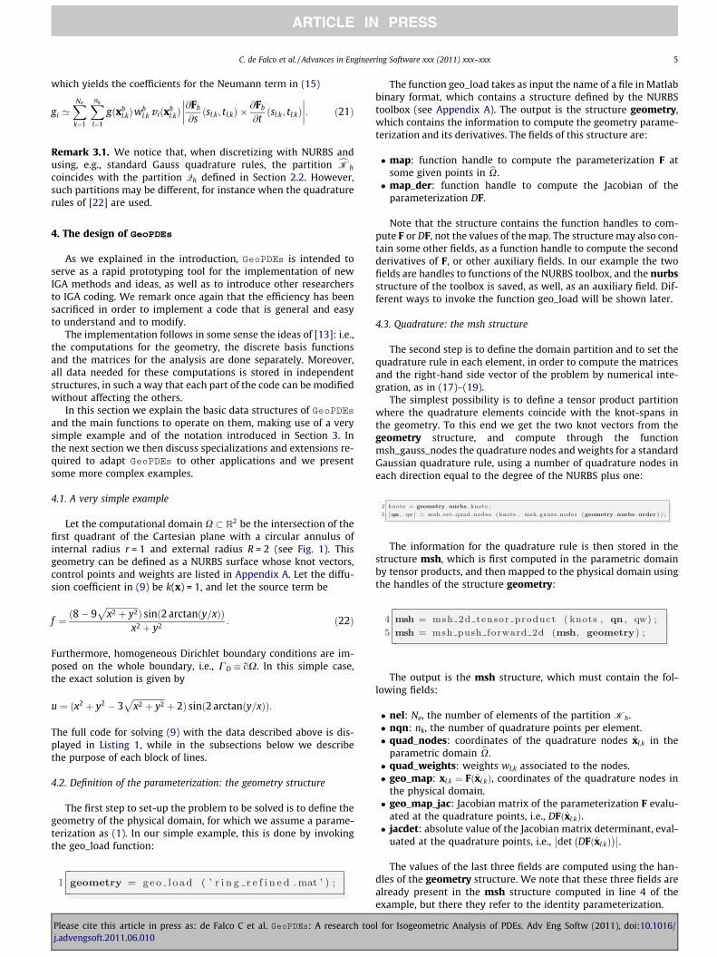
C. de Falco et al. / Advances in Engineering Software xxx (2011) xxx–xxx 5
which yields the coefficients for the Neumann term in (15)
gi ’XNe
k¼1
Xnk
l¼1
gðxbl;kÞwb
l;k v iðxbl;kÞ
@Fb
@sðsl;k; tl;kÞ �
@Fb
@tðsl;k; tl;kÞ
���� ����: ð21Þ
Remark 3.1. We notice that, when discretizing with NURBS andusing, e.g., standard Gauss quadrature rules, the partition cKh
coincides with the partition Qh defined in Section 2.2. However,such partitions may be different, for instance when the quadraturerules of [22] are used.
4. The design of GeoPDEs
As we explained in the introduction, GeoPDEs is intended toserve as a rapid prototyping tool for the implementation of newIGA methods and ideas, as well as to introduce other researchersto IGA coding. We remark once again that the efficiency has beensacrificed in order to implement a code that is general and easyto understand and to modify.
The implementation follows in some sense the ideas of [13]: i.e.,the computations for the geometry, the discrete basis functionsand the matrices for the analysis are done separately. Moreover,all data needed for these computations is stored in independentstructures, in such a way that each part of the code can be modifiedwithout affecting the others.
In this section we explain the basic data structures of GeoPDEsand the main functions to operate on them, making use of a verysimple example and of the notation introduced in Section 3. Inthe next section we then discuss specializations and extensions re-quired to adapt GeoPDEs to other applications and we presentsome more complex examples.
4.1. A very simple example
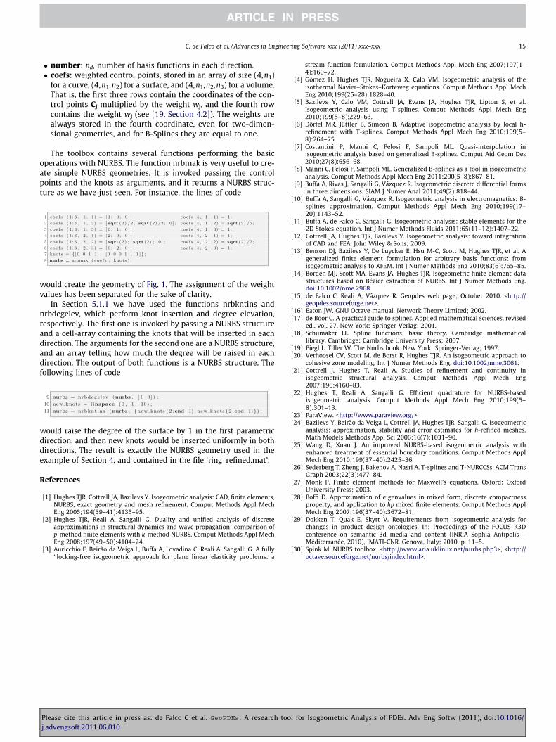
Let the computational domain X � R2 be the intersection of thefirst quadrant of the Cartesian plane with a circular annulus ofinternal radius r = 1 and external radius R = 2 (see Fig. 1). Thisgeometry can be defined as a NURBS surface whose knot vectors,control points and weights are listed in Appendix A. Let the diffu-sion coefficient in (9) be k(x) = 1, and let the source term be
f ¼ ð8� 9ffiffiffiffiffiffiffiffiffiffiffiffiffiffiffix2 þ y2
pÞ sinð2 arctanðy=xÞÞ
x2 þ y2 : ð22Þ
Furthermore, homogeneous Dirichlet boundary conditions are im-posed on the whole boundary, i.e., CD � oX. In this simple case,the exact solution is given by
u ¼ ðx2 þ y2 � 3ffiffiffiffiffiffiffiffiffiffiffiffiffiffiffix2 þ y2
pþ 2Þ sinð2 arctanðy=xÞÞ:
The full code for solving (9) with the data described above is dis-played in Listing 1, while in the subsections below we describethe purpose of each block of lines.
4.2. Definition of the parameterization: the geometry structure
The first step to set-up the problem to be solved is to define thegeometry of the physical domain, for which we assume a parame-terization as (1). In our simple example, this is done by invokingthe geo_load function:
Please cite this article in press as: de Falco C et al. GeoPDEs: A research tooj.advengsoft.2011.06.010
The function geo_load takes as input the name of a file in Matlabbinary format, which contains a structure defined by the NURBS
toolbox (see Appendix A). The output is the structure geometry,which contains the information to compute the geometry parame-terization and its derivatives. The fields of this structure are:� map: function handle to compute the parameterization F atsome given points in bX.� map_der: function handle to compute the Jacobian of the
parameterization DF.
Note that the structure contains the function handles to com-pute F or DF, not the values of the map. The structure may also con-tain some other fields, as a function handle to compute the secondderivatives of F, or other auxiliary fields. In our example the twofields are handles to functions of the NURBS toolbox, and the nurbsstructure of the toolbox is saved, as well, as an auxiliary field. Dif-ferent ways to invoke the function geo_load will be shown later.
4.3. Quadrature: the msh structure
The second step is to define the domain partition and to set thequadrature rule in each element, in order to compute the matricesand the right-hand side vector of the problem by numerical inte-gration, as in (17)–(19).
The simplest possibility is to define a tensor product partitionwhere the quadrature elements coincide with the knot-spans inthe geometry. To this end we get the two knot vectors from thegeometry structure, and compute through the functionmsh_gauss_nodes the quadrature nodes and weights for a standardGaussian quadrature rule, using a number of quadrature nodes ineach direction equal to the degree of the NURBS plus one:
The information for the quadrature rule is then stored in the
structure msh, which is first computed in the parametric domainby tensor products, and then mapped to the physical domain usingthe handles of the structure geometry:The output is the msh structure, which must contain the fol-lowing fields:
� nel: Ne, the number of elements of the partition Kh.� nqn: nk, the number of quadrature points per element.� quad_nodes: coordinates of the quadrature nodes xl;k in the
parametric domain bX.� quad_weights: weights wl,k associated to the nodes.� geo_map: xl;k ¼ Fðxl;kÞ, coordinates of the quadrature nodes in
the physical domain.� geo_map_jac: Jacobian matrix of the parameterization F evalu-
ated at the quadrature points, i.e., DFðxl;kÞ.� jacdet: absolute value of the Jacobian matrix determinant, eval-
uated at the quadrature points, i.e., det DFðxl;kÞ� ��� ��.
The values of the last three fields are computed using the han-dles of the geometry structure. We note that these three fields arealready present in the msh structure computed in line 4 of theexample, but there they refer to the identity parameterization.
l for Isogeometric Analysis of PDEs. Adv Eng Softw (2011), doi:10.1016/

6 C. de Falco et al. / Advances in Engineering Software xxx (2011) xxx–xxx
4.4. The discrete space: the space structure
The most important structure of our implementation is the onereferred to as space. This contains the information regarding thebasis functions of the discrete space Vh, and their evaluation atthe quadrature nodes in order to numerically compute the inte-grals of the problem.
In our example we are invoking the isoparametric paradigm,which means that the space of the geometry and the discrete spaceof the shape functions coincide. Hence, the information for the dis-crete space is already contained in the nurbs structure of theNURBS toolbox, that we stored as a field in geometry. The newstructure is computed using this information and the msh struc-ture with the command:
As in FEM, the basis functions in IGA are locally supported, thusthe integrals on each element of the partition are only computed
for a reduced number of basis functions. Accordingly, only the val-ues of some basis functions are stored on each element. Analo-gously to what is done in FEM, a global numbering of the basisfunctions is introduced. Then, for each element of the quadraturepartition we give its connectivity, that is, the number associatedto the basis functions whose support intersects the element. There-fore, the information contained in the structure is the following:� ndof: Nh, total number of degrees of freedom, which is equal tothe dimension of the space Vh.� nsh: Ns, number of non-vanishing basis functions in each
element.� connectivity: numbers associated to the basis functions that do
not vanish on each element. It has size Ns � Ne, where Ne is thenumber of elements.� shape_functions: evaluation of the basis functions at the quad-
rature points, that is, the quantities vi(xl,k) in Eq. (19). In ourmodel problem, its size is nk � Ns � Ne, where nk is the numberof quadrature points.� spfun: function handle to evaluate the fields above at the points
given in a msh structure, this is used when evaluating at points dif-ferent from the quadrature points is required, e.g. for visualization.
Some optional fields may also appear, depending on the problemto be solved. For instance, in our model problem we also need the field
Fig. 1. Solution of the model problem.
Please cite this article in press as: de Falco C et al. GeoPDEs: A research tooj.advengsoft.2011.06.010
� shape_function_gradients: gradient of the basis functionsevaluated at the quadrature points, that is, grad vi(xl,k). In ourmodel problem it has size d � nk � Ns � Ne, where d is the dimen-sion of the problem.
In the example, the values of the shape functions and their gra-dients are first computed in the parametric domain, making use ofsome functions of the NURBS toolbox. The values of the gradientsin the physical domain are then computed by applying the push-forward, using the information contained in msh.
We will see later other examples where fields for the divergenceor the curl are also computed. Moreover, we notice that the struc-ture contains another field called boundary, that will be explainedin Section 4.6.
4.5. Matrix and vector construction
Once the three basic data structures have been initialized, thenext step is to assemble the stiffness matrix and the right-handside of the linear system. GeoPDEs provides several functions thatallow to compute the matrices and right-hand sides for differentPDE problems, starting from the msh and space structures intro-duced above. These functions all have a very similar structure,which may be adapted with very little changes to handle differentdifferential problems.
Recalling that in our problem k(x) = 1, and the source function fis given by (22), the stiffness matrix and the right-hand side arecomputed with the commands
where the last input arguments in lines 8 and 9 are the coefficientsk(x) and f(x), respectively, evaluated at the quadrature points. Inline 8 the space structure is passed twice, because the function isprepared to use different spaces for trial and test functions.
Remark 4.1. In line 7, two rather advanced commands of theMatlab programming language appear: the function deal is used tocompactly do multiple assignments in one single line, and thefunction squeeze to remove the singleton dimensions of multi-dimensional arrays. Although we have tried to keep the program-ming style of GeoPDEs as simple as possible, the extensive use ofmulti-dimensional arrays and tensor-product meshes and spaceshas made it necessary to resort to other advanced constructs (e.g.,repmat or reshape). However, the detailed description of suchcommands is beyond the scope of the present paper and we referthe interested reader to the Matlab or Octave manuals.
The separation of the matrix assembly stage from that of basisfunction definition and evaluation is one of the main features ofour code, which directly descends from its design objectives. Inchoosing to evaluate and store all the values of the basis functionsat time of initialization of the space structure we have clearly fa-vored speed in the trade-off with memory consumption. Althoughthis choice limits the maximum size of problems that GeoPDEs canhandle, the actual limit being dependent on available hardware,this bottleneck may be overcome, e.g., by changing the fields ofspace structure to be function handles rather than arrays. Anyway,since the handling of problems of such size is beyond the scope ofthis presentation we do not further pursue this issue here.
l for Isogeometric Analysis of PDEs. Adv Eng Softw (2011), doi:10.1016/

C. de Falco et al. / Advances in Engineering Software xxx (2011) xxx–xxx 7
To show how our approach simplifies the implementation, wereport below (Listing 2) a simple Octave function to compute themass matrix in (16), using Eq. (19). It takes as arguments the spaceand msh structures, and the coefficient � already evaluated at thequadrature points. The function basically consists of a cycle overthe elements, two cycles over the basis functions, and a final cycleover the quadrature points of each element.
Remark 4.2. The function of Listing 2 slightly differs from the oneactually present in the package. The latter, in fact, allows the use ofdifferent spaces for trial and test functions, and is valid for bothscalar and vectorial problems. Other minor changes were done tomake the function faster in Matlab.
4.6. The treatment of boundary conditions: the boundarysubstructures
The imposition of homogeneous boundary conditions in IGA isstraightforward. In fact, homogeneous Neumann conditions areautomatically imposed without any change in the arrays (as inFEM). For homogeneous Dirichlet conditions, as in our example,we first need to identify the boundary degrees of freedom corre-sponding to functions that do not vanish on the boundary, and sep-arate them from the internal degrees of freedom. This is done inthe code with the commands
Then, the coefficients aj in (14) for the internal degrees of free-
dom are computed as the solution of the linear system, whereas forthe boundary ones they are set to zero:For the implementation of boundary conditions, both the mshand the space structures are enriched with a field called bound-
ary. In order to define these fields we first divide the boundaryListing 2. Matlab function to c
Please cite this article in press as: de Falco C et al. GeoPDEs: A research tooj.advengsoft.2011.06.010
of the parametric domain bX into a certain number of sides.Then, the boundary field is defined as an array that contains,for each side, a msh or a space structure, similar to the onespreviously defined: msh.boundary contains a partition of eachboundary side in order to perform numerical integration (mostlyinherited from the one defined on the whole domain), whilespace.boundary contains information about the boundary basisfunctions, and their values at the quadrature points given bymsh.boundary.
There are, however, small differences with respect to the origi-nal structures we introduced before. In the msh.boundary struc-ture, the field jacdet does not longer contain the determinant ofthe Jacobian. Instead, it contains the norm of the differential ofthe boundary parameterization Fb, which is the term F0bðtl;kÞ
�� �� in(20) or @Fb
@s ðsl;k; tl;kÞ � @Fb@t ðsl;k; tl;kÞ
��� ��� in (21). The structure also containsthe field normal, with the value of the unit normal exterior vectorat the boundary quadrature points.
In space.boundary the ndof and connectivity fields refer to alocal numbering of the basis functions actually supported on eachboundary side. Therefore, it is also necessary to include the fielddofs, which relates this local numbering to the global numberingin the whole domain. This field is in fact the one we have used inthe example to determine which degrees of freedom had to beset to zero.
Obviously, an example with homogeneous boundary conditionsis not the best suited to explain the boundary substructures, butits use will be made clearer in Section 5.1.4, where we solve a mod-el problem with non-homogeneous boundary conditions.
4.7. Postprocessing: visualization and computation of the error
Once the linear system has been solved, the last step is to visu-alize the computed solution. As IGA is seen as a tool to improve thecommunication between CAD software and PDE discrete solvers,the same holds for the communication between the solvers andthe visualization software. We are far from being experts on thematter, so our immediate goal is not to implement new techniquesto do it. Instead, we have decided to use an already existing soft-ware (namely, ParaView [23]) and prepare a function to visualizeour solution data with it.
ompute the mass matrix.
l for Isogeometric Analysis of PDEs. Adv Eng Softw (2011), doi:10.1016/

Listing 1. Solving the model problem with GeoPDEs.
8 C. de Falco et al. / Advances in Engineering Software xxx (2011) xxx–xxx
The following command evaluates the solution of the problemat the points given by a 20 � 20 grid, uniform in the parametric do-main, and saves the results in a vtk structured data file format,that can be visualized with ParaView.
The resulting plot is reported in Fig. 1. Other examples provided
with the package also show how to plot the solution in Octave orMatlab using sp_eval_2d.This handle allows to evaluate the shape functions of the dis-crete space, and also their gradients, at a set of given points (notnecessarily being the quadrature points). The same function is usedwhenever the solution must be computed at a set of points. For in-stance, in academical cases in which we know the exact solution,the L2–norm of the error is computed as
where the last argument is a function handle to compute the exact
solution. The function sp_l2_error also makes use of the handlespfun mentioned above.5. Applying GeoPDEs to more complex problems
The sequence of steps of the previous section represents the ba-sic structure of a script to solve a PDE problem with GeoPDEs. Inthe first part of this section we show possible modifications of thisstructure, to tackle more complex and interesting examples. In thesecond part of the section we show the main modifications thathave to be done in order to solve problems in linear elasticity, fluidmechanics and electromagnetism.
5.1. Modifications of the model problem
We start by introducing minor modifications to Listing 1, in or-der to solve the same problem with different approaches. This willallow us to show how the code can be easily modified.
5.1.1. Introducing h-, p- and k-refinementIn the simple example of the previous section we solved the
problem by loading a geometry from the NURBS toolbox, and then
Please cite this article in press as: de Falco C et al. GeoPDEs: A research tooj.advengsoft.2011.06.010
performed the discretization of the problem exactly in the samespace in which the geometry was defined. But for real problemsit is necessary to introduce a refined discrete space in order toget accurate numerical solutions. One of the advantages of IGAwith respect to FEM is that the refinement can be done withoutaffecting the geometry, and for NURBS and B-Splines it is imple-mented in an easy manner. In this section we explain how the h-, p- and k-refinements are treated in GeoPDEs. In all the three caseswe make use of functions contained in the NURBS toolbox (seeAppendix A). We refer the reader to the ‘‘help’’ of these functionsfor more details, and to [19] for the definition of the concepts of de-gree elevation and knot insertion that are used in what follows.
The case of p-refinement is the easiest to explain. In this casethe refinement consists on applying degree elevation, which isdone by invoking the nrbdegelev function of the toolbox. For in-stance, in order to solve with NURBS of degree 5, the followingcommands should be added between lines 1 and 2 of Listing 1:
The purpose of the second line is to avoid executing degree ele-
vation when the desired degree is lower than the actual one of thegeometry, a useful check when automatic refinement proceduresare implemented.h-refinement is instead obtained by knot insertion, which is easilycomputed using the function nrbkntins of the toolbox. The importantthing is to determine which knots one would like to insert. A simpleand classical strategy is to add new knots uniformly, for which thefunction kntrefine of the toolbox can be helpful. For instance, substi-tuting the lines 2 and 3 of the p-refinement example by:
would insert two new knots in each subinterval of the original knot
vectors. The last argument is used to specify the desired continuity,so in this case the new knots are added with the right multiplicity toget a discrete space of C0 continuity.l for Isogeometric Analysis of PDEs. Adv Eng Softw (2011), doi:10.1016/

C. de Falco et al. / Advances in Enginee
Finally, k-refinement consists of performing first a degree eleva-tion, and then a knot insertion with the lowest multiplicity for thenew knots, in order to have higher regularity of the basis functions.The implementation is an easy combination of what is done for p-and h-refinement. In the following example the problem is besolved with NURBS of degree 3, and each interval of the originalknot vector is refined by inserting one new knot without repeti-tions, which yields C2 continuity at these knots:
Notice that in these examples the function geo_load is invokedwith a NURBS structure, rather than with a binary file. In the next
section we will give more details about this function.5.1.2. Implementation of the non-isoparametric approachOne of the main features of GeoPDEs is the fact that the geom-
etry and the discrete space are treated independently. This allowsto solve problems using non-isoparametric approaches, where thesolution space does not coincide with the geometry space.
The computation with B-Spline spaces is easily implemented,and very similar to NURBS. In order to solve with a NURBS geom-etry but with a spline discretization, the example given in Listing 1is modified by substituting line 6 with
where 4 is the degree of the B-Spline space associated to the knot
vectors. In fact, the knot vectors for the geometry and for the discretespace are not necessarily the same, which means that geometryrefinement can be avoided. We however remark that the continuityof the B-Spline space must be related to the continuity of the geom-etry in order to obtain optimal convergence rates (see [10,24]).Since the geometry and the discrete space are unrelated, differ-ent ways of representing the geometry can be considered, as far asthe geometry is given by a parameterization in the form of (1), anda geometry structure as that described in Section 4 can be defined.The function geo_load is prepared to create the structure for geom-etries defined in the following ways:
� As a structure of the NURBS toolbox, either from a file or from avariable.� As an affine transformation, defined by a 4x4 matrix.� As a function handle explicitly defined by the user.
In this latter case the user must provide the Matlab functions tocompute the parameterization and its derivatives. Let us show thiswith an example. We consider the same problem as in Section 4,but with the domain defined by F(u,v) = ((u + 1)cos (pv/2), (u + 1)sin(pv/2)), with 0 < u, v < 1. Accordingly, the parameteri-zation is defined through the following Matlab function:
Please cite this article in press as: de Falco C et al. GeoPDEs: A research tooj.advengsoft.2011.06.010
and its Jacobian matrix by:
Then, the geometry structure may be computed using the fol-
ring Software xxx (2011) xxx–xxx 9
lowing command:
As the knot vector for the solution B-Spline space cannot in this
case be taken from the geometry, the user must generate one, be-fore calling the msh and space constructors. As an example, the fol-lowing call uses the kntuniform function from the nurbs toolbox togenerate a uniform knot vector with nine knotspans (ten breaks)for basis functions of degree two and regularity one:Apart from the modifications above the rest of the script re-
mains identical to that of Listing 1.5.1.3. Introducing other modifications: a different quadrature ruleAs already noted in Remark 3.1, although in many cases they
coincide, the partition of the domain bX used for quadrature, cKh,and the Cartesian partition Qh induced by the knot vectors of thesolution function space Vh are, in general, different. One simpleyet notable example where selecting the elements of cKh so thatthey do not coincide with those of Qh is the case where the quad-rature rules on macro–elements introduced in [22] are used to re-duce the total number of quadrature nodes by exploiting thehigher smoothness of the B-Spline basis functions. In this particu-lar case, each element of cKh is the union of a few neighboring cellsin Qh. Implementing this approach is particularly simple in GeoP-
DEs where the definition of the domain partition is independent ofthe definition of the function space. To clarify this with an example,we solve the same problem as in Section 5.1.2 using a quadraturerule that integrates exactly functions of ðS4
0Þ2 on 3 neighboring knot
spans (this rule is given in Table 9 of [22] and is reported in Table 1below for convenience). The nodes and weights of the quadraturerule need to be stored in the rows of a matrix as:
Using the same knot vector as in Section 5.1.2 above, we can de-fine the breaks for the partition cKh simply eliminating the redun-
dant ones:We can then proceed to assemble the msh structure with the
following linel for Isogeometric Analysis of PDEs. Adv Eng Softw (2011), doi:10.1016/
10 C. de Falco et al. / Advances in Engineering Software xxx (2011) xxx–xxx
where the last input argument specifies that the quadrature
rule is defined on the interval [0, 1]. Again, apart from themodifications above, the rest of the script remains identical to thatof Listing 1.5.1.4. Implementation of non-homogeneous boundary conditionsThe previous examples had the only purpose of explaining the
code and the construction of the different structures on which itis based, but we only considered a problem with homogeneousboundary conditions. We now address how to implement non-homogeneous boundary conditions of both Neumann and Dirichlettype using the boundary substructures of Section 4.6.
Let us consider the same domain X of Section 4, with theboundary parts CN = {(x,y): 0 6 x 6 1,y = 0} and CD = @XnCN. Letus assume that the coefficient k(x) is constant and equal to one.Then, the problem
�Du ¼ 0 in X;@u@n ¼ g ¼ �ex cosðyÞ on CN ;
u ¼ h ¼ ex sinðyÞ on CD;
8><>: ð23Þ
has exact solution u = ex sin(y). Since the source term is equal tozero, the first modification to introduce in Listing 1 is to substituteline 9 by:
The exact solution has to be changed as well, so the line 15 now
reads:In order to apply the boundary conditions it is necessary to
determine which kind of condition has to be applied on each sideof the domain. This is done through the arrays nmnn_sides anddrchlt_sides, that must be supplied by the user. Then we recall thatthe structure msh.boundary contains all the information for aquadrature rule defined on the boundary, and that space.bound-ary contains the information about the boundary functions andtheir values at the quadrature points. Using these structures, thecomputation of the Neumann condition is included after line 9 ofListing 1 as follows:That is, for each boundary with a Neumann condition, we first
evaluate the function g at the quadrature points of the boundarypartition. Then, the boundary term appearing in (10) is computedusing the function op_f_v, which is the same as for the source term,but is invoked here with the fields defined on the boundary. Final-ly, the assembling of the global right-hand side is done by using thefield dofs, already explained in Section 4.6.The implementation of the Dirichlet boundary condition in IGAis not trivial, and it is still a matter of research (see [7,25]). For ourexamples we have imposed the condition by means of an L2–pro-jection of the boundary data. The method is neither local nor effi-
Please cite this article in press as: de Falco C et al. GeoPDEs: A research tooj.advengsoft.2011.06.010
cient, but it provides a good example to show how the structures ofthe code can be used. The following piece of code should substitutelines from 10 to 12 in Listing 1:
The first four lines identify the degrees of freedom on the Dirich-
let boundary, and provide the needed initializations. Lines 6 and 7are inserted only for the sake of clarity. Then, for each Dirichletboundary we compute the value of the function h at the quadraturepoints, by using the information of the boundary fields. From lines11 to 14 the matrix and the right-hand side are assembled to com-pute the L2–projection, which is done in line 17. Finally, the right-hand side of the problem is corrected on line 18.5.2. Linear elasticity
The present section is devoted to discussing how GeoPDEs canbe utilized to solve structural mechanics problems, which repre-sent one of the first and, up to now, most prominent applicationsof IGA.
As in the sections above, we choose a reference problem and gothrough the steps to solve it with GeoPDEs. In particular, let usconsider the case of a linear, elastic, isotropic body filling the re-gion X � Rd; d ¼ 2;3, with a part CD of its boundary being keptfixed while a distributed load g is applied on the remaining partof the boundary CN. The displacement u of the elastic body is givenby the solution of the problem:
Find u 2 V ¼ H10;CDðXÞ
� dsuch thatZ
X2l�ðuÞ : �ðvÞ þ kdivðuÞdivðvÞð Þ ¼
ZX
f � v þZ
CN
g � v 8v 2 V ;
ð24Þ
where k and l are the Lamé parameters of the material and �(u) isthe strain tensor, which is the symmetric part of the displacementgradients. For d = 2, this represents a problem in the plane strainregime.
The main peculiarity of (24) in comparison to the model prob-lem considered up to now is that the space V, and its finite dimen-sional approximant Vh, are now spaces of vector-valued functions.Constructing a vector-valued function space in GeoPDEs is quitestraightforward. For example, in the case d = 3 one first computes,in the same manner we have seen in Section 4, the msh structureand the space structures spx, spy and spz, to which the compo-nents of the displacement belong. The vector-valued space struc-ture is then computed as
The main difference of the new structure sp with the one we
have seen in Section 4.4, is that the fields sp.shape_functionsand sp.shape_function_gradients have size d � nk � Ns � Ne, andd � d � nk � Ns � Ne, respectively. Each basis function in the new spacel for Isogeometric Analysis of PDEs. Adv Eng Softw (2011), doi:10.1016/
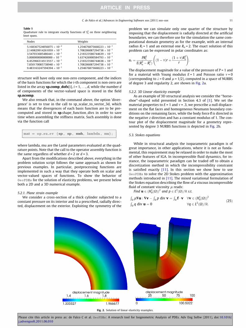
Table 1Quadrature rule to integrate exactly functions of S4
0 on three neighboringknot spans.
Nodes Weights
5.168367524056075 � 10�2 1.254676875668223 � 10�1
2.149829914261059 � 10�1 1.708286087294738 � 10�1
3.547033685486441 � 10�1 1.218323586744639 � 10�1
5.000000000000000 � 10�1 1.637426900584793 � 10�1
6.452966314513557 � 10�1 1.218323586744638 � 10�1
7.850170085738940 � 10�1 1.708286087294738 � 10�1
9.483163247594394 � 10�1 1.254676875668223 � 10�1
C. de Falco et al. / Advances in Engineering Software xxx (2011) xxx–xxx 11
structure will have only one non-zero component, and the indicesof the basis functions for which the i-th component is non-zero arelisted in the array sp.comp_dofs{i}, i = 1, . . ., d, while the number dof components of the vector-valued space is stored in the fieldsp.ncomp.
We also remark that, in the command above, the option ’diver-gence’ is set to true in the call to sp_scalar_to_vector_3d, whichmeans that the divergences of each basis function are to be pre-computed and stored in sp.shape_function_divs in order to savetime when assembling the stiffness matrix. Such assembly is donevia the function call
where lambda, mu are the Lamé parameters evaluated at the quad-
rature points. Note that the call to the operator assembly function isthe same regardless of whether d = 2 or d = 3.Apart from the modifications described above, everything in theproblem solution script follows the same approach as shown forprevious examples. In particular, postprocessing functions areimplemented in such a way that they operate both on scalar andvector-valued spaces of functions. To show the behavior ofGeoPDEs for the solution of elasticity problems, we present belowboth a 2D and a 3D numerical example.
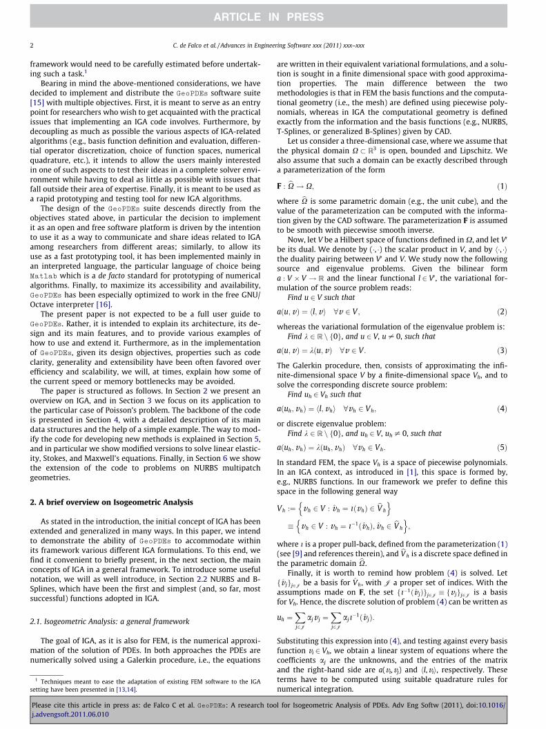
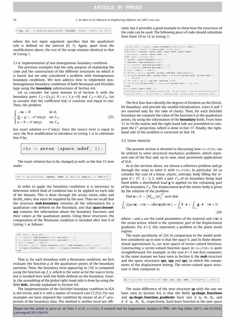
5.2.1. Plane strain exampleWe consider a cross-section of a thick cylinder subjected to a
constant pressure on its interior and to a prescribed, radially direc-ted, displacement on the exterior. Exploiting the symmetry of the
Fig. 2. Solution of linear
Please cite this article in press as: de Falco C et al. GeoPDEs: A research tooj.advengsoft.2011.06.010
problem we can simulate only one quarter of the structure byimposing that the displacement is radially directed at the artificialboundaries, we can therefore use for the simulation the same com-putational domain geometry as for the example, with an internalradius Ri = 1 and an external one Ro = 2. The exact solution of thisproblem can be expressed in polar coordinates as:
ur ¼PR2
i
EðR2o � R2
i Þð1� mÞr þ ð1þ mÞR2
o
r
!:
The displacement magnitude for a value of the pressure of P = 1 andfor a material with Young modulus E = 1 and Poisson ratio m = 0(corresponding to k = 0 and l = 1/2), computed in a space of NURBSof degree 3 and regularity 2, are shown in Fig. 2a.
5.2.2. 3D Linear elasticity exampleAs an example of 3D structural analysis we consider the ‘‘horse-
shoe’’-shaped solid presented in Section 4.3 of [1]. We set thematerial properties to E = 1 and m = .3, we prescribe a null displace-ment on the flat faces and homogeneous Neumann boundary con-ditions on the remaining faces, while the body force f is directed inthe negative z direction and has a constant modulus of 1. The con-tour plot of the displacement magnitude for a geometry repre-sented by degree 3 NURBS functions is depicted in Fig. 2b.
5.3. Stokes equations
While in structural analysis the isoparametric paradigm is ofgreat importance, in other applications, where it is not as funda-mental, this requirement may be relaxed in order to make the mostof other features of IGA. In incompressible fluid dynamics, for in-stance, the isoparametric paradigm can be traded off to obtain adiscretization method in which the incompressibility constraintis satisfied exactly [11]. In this section we show how to useGeoPDEs to solve the 2D Stokes problem with the approximationmethods introduced in [11]. The mixed variational formulation ofthe Stokes equation describing the flow of a viscous incompressiblefluid of constant viscosity l reads:
Find u 2 ðH10ðXÞÞ
2 and p 2 L2ðXÞ=R s.t.RX l$u : $v �
RX p div v ¼
RX f � v 8v 2 ðH1
0ðXÞÞ2R
X q div u ¼ 0 8q 2 L2ðXÞ=R:ð25Þ
elasticity examples.
l for Isogeometric Analysis of PDEs. Adv Eng Softw (2011), doi:10.1016/
(a) (b) (c)Fig. 3. Removal of redundant degrees of freedom of bQ RT
h .
12 C. de Falco et al. / Advances in Engineering Software xxx (2011) xxx–xxx
Three compatible pairs of discretization spaces are considered in[11] in which the discrete counterpart of (25) can be set. Recallingthe notation of Section 2.2, and assuming for simplicity that the reg-ularity a is the same at all knots, we first define a B-Spline space forthe pressure in the parametric domain as bQ h � bQ hðp;aÞ ¼ Sp;p
a;a,which will be the same for the three pairs. The discrete spaces forthe velocity are then defined, in the parametric domain, asbV TH
h ¼ Spþ1;pþ1a;a � Spþ1;pþ1
a;a ;bV RTh ¼ Spþ1;p
aþ1;a � Sp;pþ1a;aþ1;bV NDL
h ¼ Spþ1;pþ1aþ1;a � Spþ1;pþ1
a;aþ1 :
Here TH, RT and NDL stand for Taylor-Hood, Raviart-Thomas andNédélec (of the second kind) respectively, as these B-Spline spacesare consistent generalizations of the well-known finite elementspaces known by these names. As explained in [11], the way to mapthe spaces to the physical domain is different in each case. In partic-ular the TH spaces can be mapped to the physical domain X by thesame ‘‘component-wise’’ mapping used in the previous section, i.e.
VTHh ¼ v : v � F 2 bV TH
h
n o; Qh ¼ q : q � F 2 bQ h
n o: ð26Þ
The same mapping for the pressure space is used in the two otherpairs. On the other hand, to get stable discretizations, the velocityspaces for RT and NDL are transformed via a Piola-type mapping, i.e.
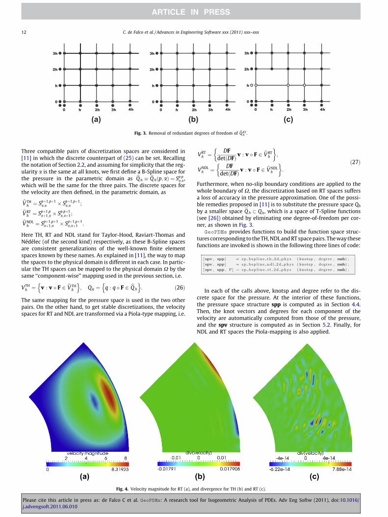
Fig. 4. Velocity magnitude for RT (a), an
Please cite this article in press as: de Falco C et al. GeoPDEs: A research tooj.advengsoft.2011.06.010
VRTh ¼
DFdetðDFÞv : v � F 2 bV RT
h
� ;
VNDLh ¼ DF
detðDFÞv : v � F 2 bV NDLh
� :
ð27Þ
Furthermore, when no-slip boundary conditions are applied to thewhole boundary of X, the discretization based on RT spaces suffersa loss of accuracy in the pressure approximation. One of the possi-ble remedies proposed in [11] is to substitute the pressure space Qh
by a smaller space eQ h � Qh, which is a space of T-Spline functions(see [26]) obtained by eliminating one degree-of-freedom per cor-ner, as shown in Fig. 3.
GeoPDEs provides functions to build the function space struc-tures corresponding to the TH, NDL and RT space pairs. The way thesefunctions are invoked is shown in the following three lines of code:
In each of the calls above, knotsp and degree refer to the dis-crete space for the pressure. At the interior of these functions,the pressure space structure spp is computed as in Section 4.4.Then, the knot vectors and degrees for each component of thevelocity are automatically computed from those of the pressure,and the spv structure is computed as in Section 5.2. Finally, forNDL and RT spaces the Piola-mapping is also applied.
d divergence for TH (b) and RT (c).
l for Isogeometric Analysis of PDEs. Adv Eng Softw (2011), doi:10.1016/

C. de Falco et al. / Advances in Engineering Software xxx (2011) xxx–xxx 13
Of particular interest is the additional output P given by the RTspace constructor, which is a matrix that operates the change of basisfrom the B-Spline space Qh to the T-Spline space eQ h. The purpose forcomputing P is that it allows to work with functions in eQ h withoutthe need of implementing a constructor for general T-Spline spaces.
As an example we consider a problem set on one eighth of anannulus, described through a NURBS parameterization, with no-slip boundary conditions on the whole domain boundary. The ex-act solution and right-hand side can be found in the filetest_stokes_annulus of the package. In Fig. 4a we show the velocitycomputed with RT elements for p = 3 and a = 1, while in Fig. 4b andc we compare the divergence of the velocity field obtained by theTH discretization scheme with that of a RT scheme with the samedegree and regularity for the pressure component of the solution.
5.4. Maxwell equations
The main interest for using IGA in electromagnetism, apart fromthe exact description of geometry, is the higher regularity of thesolution with respect to finite elements. For edge finite elements,spreadly used in computational electromagnetims, the normal com-ponent of the computed solution is discontinuous. This property isuseful to simulate problems with several materials, since the normalcomponent of the physical solution is also discontinuous, but withineach material higher regularity may be desirable. The B-Spline-based discretization introduced in [9,10], besides maintaining exactgeometry, provides more regular solutions than edge elements. Wenow show how these methods are implemented in GeoPDEs,explaining the main modifications that have to be done in order tosolve Maxwell’s eigenvalue problem. The explanation of the discret-ization scheme is extensively described in the aforementionedpapers, along with several numerical examples.
We focus here on the 3D Maxwell eigenproblem. Let X � R3 bedefined as in (1) and let its boundary be split into two disjoint parts,@X = CD [ CN. The problem with mixed boundary conditions reads:
curlðl�1curlEÞ ¼ k�E in X;
E� n ¼ 0 on CD;
l�1curlE� n ¼ 0 on CN:
8><>:The equivalent weak problem is to find an electric fieldE 2 H0;CD ðcurl; XÞ such thatZ
Xl�1curlE � curlv ¼ k
ZX�E � v 8v 2 H0;CD ðcurl; XÞ;
with H0;CD ðcurl; XÞ the space of square integrable vectorial func-tions in X such that their curl is also square integrable, and theirtangential components are null on the boundary CD.
Fig. 5. Magnitude of the second and fifth eigen
Please cite this article in press as: de Falco C et al. GeoPDEs: A research tooj.advengsoft.2011.06.010
Using the notation of Section 2.2, and assuming again that themultiplicity is the same for all internal knots, the discrete spacein the parametric domain bX is taken equal tobV h :¼ Sp1�1;p2 ;p3
a1�1;a2 ;a3� Sp1 ;p2�1;p3
a1 ;a2�1;a3� Sp1 ;p2 ;p3�1
a1 ;a2 ;a3�1:
This belongs to a sequence of discrete spaces that, along with theircontinuous counterparts, form a commuting De Rham diagram (see[9]). The discrete space in the physical domain is then defined byusing a curl conserving transformation [27, Section 3.9], in the form
Vh ¼ u : ðDFÞTðu � FÞ 2 bV h
n o:
For the implementation, the geometry and msh structures are com-puted exactly as in all the previous problems. The only differences ap-pear in the structure space. This is constructed with the commands:
where the first line automatically constructs the knot vectors and
degrees for every component of the product space Vh, and the sec-ond one constructs the new space structure. Internally, this func-tion first builds the structure in the parametric domain in thesame fashion we explained in Section 5.2, and then applies thecurl-conserving transform, similarly to what done in Section 5.3for the Piola transform.The resulting structure is roughly the same we have seen for theother vectorial problems, the main difference being that it includesthe field shape_function_curls, which has size equal to3 � nk � Ns � Ne. The second important difference is that, since theboundary conditions just involve the tangential components ofthe solution, only the shape functions for the tangential compo-nents are stored in the boundary field.
After the construction of the structure, the matrices are assem-bled in the same manner we have seen for previous problems,using the commands
where mu and epsilon are the values of the physical parameters
evaluated at the quadrature points. The eigenvalue problem is thensolved by using the eig command from Matlab or Octave.The postprocessing part is also analogous to what we have ex-plained before. In Fig. 5 we show the magnitude of the secondand fifth eigenfunctions in a three quarters of the cylinder, with
functions in three quarters of the cylinder.
l for Isogeometric Analysis of PDEs. Adv Eng Softw (2011), doi:10.1016/

14 C. de Falco et al. / Advances in Engineering Software xxx (2011) xxx–xxx
@X = CD. In this case the geometry is exactly constructed with onlythree elements.
Finally, we would like to remark that the code includes exam-ples for different formulations of the eigenvalue problem (see[28]), and for the source problem with non-homogeneous bound-ary conditions.
Remark 5.1. The 2D and the 3D cases are a little bit different, sincein the former we have two different differential operators: curl andcurl. The operator curl acts on scalar variables and returns vector-fields, whereas the operator curl acts on vector-fields and returnsscalar variables. Something similar occurs with the tangentialboundary conditions. For this reason, some functions have differ-ent versions for the 2D and the 3D cases.
6. The treatment of NURBS multipatch conforming geometries
We have included in the code a small package to deal with mul-tipatch geometries. For this we have always assumed that thepatches are compatible, in the sense that the meshes and controlpoints must coincide on the interface, even after refinement. Moresophisticated approaches, allowing for different refinements oneach patch, can be found in [12, Chapter 3].
Let us assume that the domain X is formed by the union of np
disjoint subdomains, or patches, in the form X ¼ [np
l¼1Xl, withXl \Xl0 ¼ ;;8l – l0. Each patch is defined, analogously to (8), asFl : bX ! Xl, with bX being always the unit square or cube. We re-quire that the patches match conformingly, in the sense that, ifXi and Xj are two patches with a common interfaceCij ¼ Xi \Xj – ;, and Qi
h; Qjh are their respective meshes, then they
must coincide on the interface, i.e., QihjCij¼ Qj
hjCij, with the same
multiplicity for the corresponding knots.Since the meshes are the same, the basis functions are also the
same for both patches. Hence, it is sufficient to define a connectiv-ity array, which identifies the matching basis functions on eachpatch with one single function in the global domain (see [12]). Inorder to define this connectivity, we have made use of the data for-mat for multipatch geometries proposed in [29].
Let us start with the 2D case. For each interface we must know:the number of the two patches, the numbers of the coincidingboundary surfaces on each patch, and a flag telling if the paramet-ric direction on the first patch coincides with the parametric direc-tion on the second. The first numbers let us know, for each patch,which degrees of freedom do not vanish on the interface (stored inboundary.dofs). The flag tells us whether the degrees of freedommatch automatically, or if those of the second patch must be reor-dered (using the fliplr command).
In the 3D case, instead, the information we need for each inter-face is the following: the number of the two patches, and of theirmatching boundaries, a flag telling if the first parametric coordinateon the first surface coincides with the first parametric coordinate ofthe second surface, and two flags telling if each parametric directioncoincides. Using the first numbers, we recover the degrees of free-dom for each patch from boundary.dofs, and rewrite them in theform of two matrices. The first flag tells if the second matrix shouldbe transposed, whereas the two other flags let us know if the degreesof freedom in this matrix should be reordered, one with the fliplrcommand and the other with the flipud command.
Remark 6.1. Dealing with multipatch geometries for vector fieldapproximations is a little bit more complicated. In particular, whenapplying the curl-conserving or Piola transforms, it is necessary todefine an orientation for the tangential and the normal compo-nents, respectively. However, this is not much different from whatis done for edge and face finite elements.
Please cite this article in press as: de Falco C et al. GeoPDEs: A research tooj.advengsoft.2011.06.010
7. Conclusion
In this paper, we have presented the design philosophy andmain features of GeoPDEs, a suite of free software tools for appli-cations on Isogeometric Analysis. A first goal of GeoPDEs is to con-stitute an entry point for researchers interested in the practicalissues related to the implementation of an IGA code, while anotherimportant aim is to provide a rapid prototyping and testing tool forthe development of novel IGA algorithms.
With these main objectives in mind, we have tried to explain allbasic features and capabilities of GeoPDEs on a simple model prob-lem (i.e., Poisson), showing also how to use the code as a startingpoint to develop new IGA methods to be applied to different engi-neering fields. For instance, applications to elasticity, Stokes andMaxwell problems have been discussed and the solution of somenumerical examples has been shown. Moreover, among the differ-ent topics related to the use and possible extension of GeoPDEscovered in this paper, we have considered in particular some deli-cate issues such as h–, p–, or k–refinement strategies, boundarycondition imposition, implementation of non-isoparametric meth-ods, use of different quadrature strategies, treatment of multipatchgeometries.
As a conclusion, we believe that the present work, along withthe release of the GeoPDEs suite, may complement the literatureon IGA (see, e.g., [12] and references therein), constituting on onehand an important tool for people meeting IGA for the first timeand on the other hand the basis for the rapid development ofnew IGA ideas and applications.
Acknowledgments
The authors were partially supported by the European ResearchCouncil through the FP7 Ideas Starting Grant 205004: GeoPDEs –Innovative compatible discretization techniques for Partial DifferentialEquations. A. Reali was partially supported by the European Re-search Council through the FP7 Ideas Starting Grant 259229: ISOBIO– Isogeometric Methods for Biomechanics. This support is gratefullyacknowledged. The authors also wish to thank M. Bercovier,A. Buffa, T.J.R. Hughes and G. Sangalli, for many fruitful discussionsduring the preparation of this work.
Appendix A. The NURBS toolbox
For the description of NURBS geometric entities, and also for thecomputation of the shape functions, we use the NURBS toolbox,originally implemented in MATLAB by Mark Spink [30]. The originaltoolbox was mainly developed for the construction of NURBScurves and surfaces, based on the algorithms of [19]. In order todeal with three-dimensional problems in IGA, we have extendedsome of the basic algorithms to trivariate NURBS. The new versioncan be found in the svn repository of the Octave-Forge (http://octave.sourceforge.net) project, and it is still compatible with Matlab. We give now ashort explanation of the main features of the toolbox, and refer thereader to [30] for more detailed documentation.
The geometric entities in the NURBS toolbox are described by astructure, that contains all the necessary information. The mainfields of this structure are listed below, and explained using thesame notation as in Section 2.2:
� order: a vector with the order in each direction. In the splinesliterature, the B-Splines of degree p are said to have orderk = p + 1. Thus, it stores the values pd + 1.� knots: knot vectors Nd, stored as a cell array.
l for Isogeometric Analysis of PDEs. Adv Eng Softw (2011), doi:10.1016/
C. de Falco et al. / Advances in Engineering Software xxx (2011) xxx–xxx 15
� number: nd, number of basis functions in each direction.� coefs: weighted control points, stored in an array of size (4,n1)
for a curve, (4,n1,n2) for a surface, and (4,n1,n2,n3) for a volume.That is, the first three rows contain the coordinates of the con-trol points Cj multiplied by the weight wj, and the fourth rowcontains the weight wj (see [19, Section 4.2]). The weights arealways stored in the fourth coordinate, even for two-dimen-sional geometries, and for B-Splines they are equal to one.
The toolbox contains several functions performing the basicoperations with NURBS. The function nrbmak is very useful to cre-ate simple NURBS geometries. It is invoked passing the controlpoints and the knots as arguments, and it returns a NURBS struc-ture as we have just seen. For instance, the lines of code
would create the geometry of Fig. 1. The assignment of the weight
values has been separated for the sake of clarity.In Section 5.1.1 we have used the functions nrbkntins andnrbdegelev, which perform knot insertion and degree elevation,respectively. The first one is invoked by passing a NURBS structureand a cell-array containing the knots that will be inserted in eachdirection. The arguments for the second one are a NURBS structure,and an array telling how much the degree will be raised in eachdirection. The output of both functions is a NURBS structure. Thefollowing lines of code
would raise the degree of the surface by 1 in the first parametric
direction, and then new knots would be inserted uniformly in bothdirections. The result is exactly the NURBS geometry used in theexample of Section 4, and contained in the file ‘ring_refined.mat’.References
[1] Hughes TJR, Cottrell JA, Bazilevs Y. Isogeometric analysis: CAD, finite elements,NURBS, exact geometry and mesh refinement. Comput Methods Appl MechEng 2005;194(39–41):4135–95.
[2] Hughes TJR, Reali A, Sangalli G. Duality and unified analysis of discreteapproximations in structural dynamics and wave propagation: comparison ofp-method finite elements with k-method NURBS. Comput Methods Appl MechEng 2008;197(49–50):4104–24.
[3] Auricchio F, Beirão da Veiga L, Buffa A, Lovadina C, Reali A, Sangalli G. A fully‘‘locking-free isogeometric approach for plane linear elasticity problems: a
Please cite this article in press as: de Falco C et al. GeoPDEs: A research tooj.advengsoft.2011.06.010
stream function formulation. Comput Methods Appl Mech Eng 2007;197(1–4):160–72.
[4] Gómez H, Hughes TJR, Nogueira X, Calo VM. Isogeometric analysis of theisothermal Navier–Stokes–Korteweg equations. Comput Methods Appl MechEng 2010;199(25–28):1828–40.
[5] Bazilevs Y, Calo VM, Cottrell JA, Evans JA, Hughes TJR, Lipton S, et al.Isogeometric analysis using T-splines. Comput Methods Appl Mech Eng2010;199(5–8):229–63.
[6] Dörfel MR, Jüttler B, Simeon B. Adaptive isogeometric analysis by local h-refinement with T-splines. Comput Methods Appl Mech Eng 2010;199(5–8):264–75.
[7] Costantini P, Manni C, Pelosi F, Sampoli ML. Quasi-interpolation inisogeometric analysis based on generalized B-splines. Comput Aid Geom Des2010;27(8):656–68.
[8] Manni C, Pelosi F, Sampoli ML. Generalized B-splines as a tool in isogeometricanalysis. Comput Methods Appl Mech Eng 2011;200(5–8):867–81.
[9] Buffa A, Rivas J, Sangalli G, Vázquez R. Isogeometric discrete differential formsin three dimensions. SIAM J Numer Anal 2011;49(2):818–44.
[10] Buffa A, Sangalli G, Vázquez R. Isogeometric analysis in electromagnetics: B-splines approximation. Comput Methods Appl Mech Eng 2010;199(17–20):1143–52.
[11] Buffa A, de Falco C, Sangalli G. Isogeometric analysis: stable elements for the2D Stokes equation. Int J Numer Methods Fluids 2011;65(11–12):1407–22.
[12] Cottrell JA, Hughes TJR, Bazilevs Y. Isogeometric analysis: toward integrationof CAD and FEA. John Wiley & Sons; 2009.
[13] Benson DJ, Bazilevs Y, De Luycker E, Hsu M-C, Scott M, Hughes TJR, et al. Ageneralized finite element formulation for arbitrary basis functions: fromisogeometric analysis to XFEM. Int J Numer Methods Eng 2010;83(6):765–85.
[14] Borden MJ, Scott MA, Evans JA, Hughes TJR. Isogeometric finite element datastructures based on Bézier extraction of NURBS. Int J Numer Methods Eng.doi:10.1002/nme.2968.
[15] de Falco C, Reali A, Vázquez R. Geopdes web page; October 2010. <http://geopdes.sourceforge.net>.
[16] Eaton JW. GNU Octave manual. Network Theory Limited; 2002.[17] de Boor C. A practical guide to splines. Applied mathematical sciences, revised
ed., vol. 27. New York: Springer-Verlag; 2001.[18] Schumaker LL. Spline functions: basic theory. Cambridge mathematical
library. Cambridge: Cambridge University Press; 2007.[19] Piegl L, Tiller W. The Nurbs book. New York: Springer-Verlag; 1997.[20] Verhoosel CV, Scott M, de Borst R, Hughes TJR. An isogeometric approach to
cohesive zone modeling, Int J Numer Methods Eng. doi:10.1002/nme.3061.[21] Cottrell J, Hughes T, Reali A. Studies of refinement and continuity in
isogeometric structural analysis. Comput Methods Appl Mech Eng2007;196:4160–83.
[22] Hughes T, Reali A, Sangalli G. Efficient quadrature for NURBS-basedisogeometric analysis. Comput Methods Appl Mech Eng 2010;199(5–8):301–13.
[23] ParaView. <http://www.paraview.org/>.[24] Bazilevs Y, Beirão da Veiga L, Cottrell JA, Hughes TJR, Sangalli G. Isogeometric
analysis: approximation, stability and error estimates for h-refined meshes.Math Models Methods Appl Sci 2006;16(7):1031–90.
[25] Wang D, Xuan J. An improved NURBS-based isogeometric analysis withenhanced treatment of essential boundary conditions. Comput Methods ApplMech Eng 2010;199(37–40):2425–36.
[26] Sederberg T, Zheng J, Bakenov A, Nasri A. T-splines and T-NURCCSs. ACM TransGraph 2003;22(3):477–84.
[27] Monk P. Finite element methods for Maxwell’s equations. Oxford: OxfordUniversity Press; 2003.
[28] Boffi D. Approximation of eigenvalues in mixed form, discrete compactnessproperty, and application to hp mixed finite elements. Comput Methods ApplMech Eng 2007;196(37–40):3672–81.
[29] Dokken T, Quak E, Skytt V. Requirements from isogeometric analysis forchanges in product design ontologies. In: Proceedings of the FOCUS K3Dconference on semantic 3d media and content (INRIA Sophia Antipolis –Méditerranée, 2010), IMATI-CNR, Genova, Italy; 2010. p. 11–5.
[30] Spink M. NURBS toolbox. <http://www.aria.uklinux.net/nurbs.php3>, <http://octave.sourceforge.net/nurbs/index.html>.
l for Isogeometric Analysis of PDEs. Adv Eng Softw (2011), doi:10.1016/
![Shape Error Analysis of Functional Surface Based on ... · Isogeometric analysis (IGA) [18] is a method aimed at avoiding the discretization errors by using the same basis for analysis](https://img.pdfslide.us/doc/110x75/5e7b6bd3d7c5e65f99083e7a/shape-error-analysis-of-functional-surface-based-on-isogeometric-analysis-iga.jpg)


![ICES REPORT 13-03 Isogeometric Collocation: Cost ... › media › reports › 2013 › 1303.pdf · Isogeometric analysis (IGA) was introduced by Hughes and coworkers [1, 2] to bridge](https://img.pdfslide.us/doc/110x75/5f03982d7e708231d409d2ec/ices-report-13-03-isogeometric-collocation-cost-a-media-a-reports-a-2013.jpg)