Embed Size (px)
Citation preview
TECHNICAL UNIVERSITY OF DENMARK
DEPARTMENT OF MATHEMATICS
Isogeometric Analysis and Shape Optimization
in Electromagnetism
Ph.D. Thesis
Nguyen Dang Manh
February 2012


Isogeometric Analysis and Shape Optimizationin Electromagnetism
Nguyen Dang Manh
Department of Mathematics
Technical University of Denmark

Title of Thesis:Isogeometric Analysis and Shape Optimization in Electromagnetism
Ph.D. student:Nguyen Dang ManhDepartment of MathematicsTechnical University of DenmarkAddress: Matematiktorvet, Building 303S, DK-2800 Lyngby, DenmarkE-mail: [email protected]
Supervisors:Jens GravesenDepartment of MathematicsTechnical University of DenmarkAddress: Matematiktorvet, Building 303S, DK-2800 Lyngby, DenmarkE-mail: [email protected]
Anton EvgrafovDepartment of MathematicsTechnical University of DenmarkAddress: Matematiktorvet, Building 303S, DK-2800 Lyngby, DenmarkE-mail: [email protected]
Summary
In this thesis a recently proposed numerical method for solving partial differential equations,isogeometric analysis (IGA), is utilized for the purpose of shape optimization, with a particularemphasis on applications to two-dimensional design problems arising in electromagnetic appli-cations. The study is motivated by the fact that in contrast with most commonly utilized finiteelement approximations, IGA allows one to exactly represent geometries arising in computeraided design applications with relatively few variables using splines.
The following problems coming from theoretical considerations or engineering applicationsare solved in the thesis utilizing IGA:
• finding a shape having a few prescribed eigenvalues of the Laplace operator;
• shape optimization of sub-wavelength micro-antennas for energy concentration;
• shape optimization of nano-antennas for field enhancement;
• economical design of magnetic density separators.
From the point of view of method development, several heuristic approaches for extending avalid parametrization of the boundary onto the domain’s interior are examined in the thesis. Theparametrization approaches and a method for validating a spline parametrization are combinedinto an iterative algorithm for shape optimization of two dimensional electromagnetic problems.The algorithm may also be relevant for problems in other engineering disciplines.
Using the methods developed in this thesis, remarkably we have obtained antennas thatperform one million times better than an earlier topology optimization result. This shows agreat potential of shape optimization using IGA in the area of electromagnetic antenna designin particular, and for electromagnetic problems in general. Our conclusion is that IGA is wellsuited for shape optimization.
iii

Resume (in Danish)
I denne afhandling bliver en ny numerisk metode til løsning af partielle differentialligninger, iso-geometrisk analyse (IGA), benyttet til formoptimering, specielt med henblik pa to-dimensionelledesign problemer der optrder i elektromagnetiske anvendelser.
Studiet er motiveret af den kendsgerning, at i modstning til traditionelle finite elementer,tillader IGA ved brug af splines, at reprsenterer de geometrier, der optrder i “computer aideddesign” systemer eksakt og med relativ fa variable.
De følgende problemer, der dels kommer fra teoretiske overvejelser og dels fra konkreteingeniørvidenskabelige anvendelser, bliver i afhandlingen løst ved brug af IGA:
• bestem en form der har et lille antal givne værdier af Laplace operatoren;
• formoptimering af mikroantenner til energikoncentration pa omrader der er mindre endbølgelængden;
• formoptimering af nanoantenner til forstærkning af det elektromagnetisk felt;
• økonomisk design af magnetisk densitet separatorer.
Fra et metode udviklings synspunkt, bliver flere heuristiske fremgangsmader til at udvide enparametrisering fra randen til det indre af et omrade undersøgt i denne afhandling.
Disse parametriserings metoder og en metode til sikring af gyldigheden en spline parametris-ering bliver kombineret til en itterativ algoritme til formoptimering af to-dimensionele elek-tromagnetiske problemer. Algoritmen kan ogsa være relevant i andre ingeniørvidenskabeligediscipliner.
Blandt de nævnte problemer opnar vi bemærkelsesværdig nok, en antenne der er en mil-lion gange bedre end tidligere resultater af topologioptimering. Dette viser det store potentialefor brugen af IGA i formoptimering, af specielt antenner; men ogsa indenfor generelle elektro-magnetiske problemer. Vores konklusion er, at isogeometrisk analyse er særdeles velegnet tilformoptimering.
v

Preface
This thesis is submitted in partial fulfillment of the requirements for obtaining the degree ofPh.D. at the Technical University of Denmark. The Ph.D. project was funded by the TechnicalUniversity of Denmark and carried out at the Department of Mathematics during the periodFebruary 15th 2009 - February 14st 2012. Supervisors on the project were Associate ProfessorJens Gravesen and Associate Professor Anton Evgrafov from the Department of Mathematics.During the first year of the study period, Allan Roulund Gersborg from the Department of Me-chanical Engineering also acted as a supervisor for this project.
List of publications
The following research papers and manuscripts have been written during the three years of thePh.D. study
1. Nguyen D. M., A. Evgrafov, A.R. Gersborg, J. Gravesen, Isogeometric shape optimization ofvibrating membranes, Computer Methods in Applied Mechanics and Engineering, vol. 200,pp. 1343-1353, 2011.
2. J. Gravesen, A. Evgrafov, Nguyen D. M., On the sensitivities of multiple eigenvalues, Struc-tural and Multidisciplinary Optimization, vol. 44, pp. 583-587, 2011.
3. Nguyen D. M., A. Evgrafov, J. Gravesen, Shape optimization of sub-wavelength antennausing isogeometric analysis, in submission, August, 2011.
4. Nguyen D. M., A. Evgrafov, J. Gravesen, D. Lahaye, Economical designs of magnetic densityseparators using isogeometric analysis and shape optimization, in preparation, 2012.
Other publications by the author
1. Nguyen D. M., A. Evgrafov, J. Gravesen, J. S. Jensen, Isogeometric analysis toward shapeoptimization in electromagnetics, Proceedings of NSCM-23: the 23rd Nordic Seminar onComputational Mechanics, A. Erikson and G. Tibert eds., pp. 18-21, 2010.
2. J. Gravesen, A. Evgrafov, A.R. Gersborg, Nguyen D.M., P. N. Nielsen, Isogeometric analysisand shape optimization, Proceedings of NSCM-23: the 23rd Nordic Seminar on Computa-tional Mechanics, A. Erikson and G. Tibert eds., pp. 14-17, 2010.
Acknowledgments
First of all, I would like to deliver my sincere thanks to my supervisors for leading me instruc-tively to my present research field. In particular, I would like to express my deep gratitude toJens Gravesen for giving me the opportunity to develop my career at DTU and guiding me grad-ually to the world of splines, isogeometric analysis and shape optimization; from him I have
vii

learned, indeed, invaluable mathematical knowledge. Furthermore, I am grateful to Anton Ev-grafov, who has always helped me a lot from a scientific issue to a matter of the real life, andwith whom I alway enjoy every discussion. And, I would like to give special thanks to AllanR. Gersborg for conveying his enthusiasm to me and always looking after me even he has notworking at DTU recently.
Moreover, I would like to sincerely thank Sergey I. Bozhevolnyi and Morten Willatzen, Uni-versity of Southern Denmark, for teaching me further electromagnetic knowledge and encour-aging me a lot during the working period on the nano-antenna problem. I truly want to continueour collaboration in future.
Next, I would like to gratefully thank Domenico Lahaye, Delft University of Technology, forhis wonderful support to me during the time I visited the Delft University of Technology. Besidesthe scientific support in the magnetic density separator problem, I have also received invaluablehelps from him in other matters, especially his introduction of me to several post-doc positionsfrom his collaborators.
During the three years of my Ph.D. study, my work has been done with lots of helps from mycolleagues. In particular, I would like to give many thanks to my officemate Peter N. Nielsen forhelping me many times with his fluent or even expert knowledge of UNIX, FORTRAN, LATEX,English and for exchanging our daily stories. I would like to thank Vagn L. Hansen, SteenMarkvorsen, Peter Røgen, David Brander, Martin Carlsen for helping me on many occasions andcollaborating with me in teaching activities. I have received great helps from Poul-Erik Madsenwith my constant use of the department’s clusters. I would like to thank him a lot. Furthermore,I would like to thank Ole Christensen, Tom Høholdt, Peter Beelen, Ulla Louring, Wanja Andersenand Dorte Lundsgaard for making my administrative activities easier. And, my special thanksare given to all players of the department’s indoor football group who have helped me to refreshmy brain quickly.
I would like to thank all members of the TopOpt group for creating a scientifically andfriendlily “optimized” atmosphere. I especially thank Ole Sigmund, Jakob S. Jensen and MathiasStolpe for fruitful discussions on my antenna problem. In particular, I would like to thank NielsAage, DTU-Mechanics, for helping me get acquainted with the antenna problem and for hiseffort on validating one of our resulting antennas with his code. Furthermore, I would like tothank Julia Borghoff and Oded Amir for assisting me with some latex data and techniques forme to write this thesis.
I would like to use this opportunity to say that I am grateful: to my high school advisor ViDuc Cuong, High School of Bac Son, Lang Son; to my undergraduate advisor Tran Duc Long,Hanoi University of Science; to my graduate advisor Do Ngoc Diep, Institute of Mathematics,Vietnam, for building up the base for my future career.
Finally, I would like to send my deep gratitude: to my father Nguyen Dang Hieu, to mymother Le Thi Thiem and to my sister Nguyen Thi Hong for their lifetime supports to me; toDinh Thi Thao for helping me overcome many stressful occasions with her love and her dreamof a future happy family.
Kgs. Lyngby, February 2011
Nguyen Dang Manh
Contents
Summary iii
Resume (in Danish) v
Preface viiList of publications . . . . . . . . . . . . . . . . . . . . . . . . . . . . . . . . . . . . . . vii
Contents xi
Notation and abbreviation 1
Introduction 3Structure of the thesis . . . . . . . . . . . . . . . . . . . . . . . . . . . . . . . . . . . . 4
I Isogeometric analysis and shape optimization 5
1 Isogeometric analysis 71.1 B-splines . . . . . . . . . . . . . . . . . . . . . . . . . . . . . . . . . . . . . . . . . 7
1.1.1 Definition and basis properties . . . . . . . . . . . . . . . . . . . . . . . . 71.1.2 Polar form of a polynomial . . . . . . . . . . . . . . . . . . . . . . . . . . . 91.1.3 B-splines in terms of polar forms and their further properties . . . . . . . 10
1.2 Isogeometric analysis . . . . . . . . . . . . . . . . . . . . . . . . . . . . . . . . . . 131.2.1 Isogeometric analysis: Basis functions for analysis . . . . . . . . . . . . . . 131.2.2 Multiple patches: Enforcement of the C0-continuity of the numerical so-
lution . . . . . . . . . . . . . . . . . . . . . . . . . . . . . . . . . . . . . . 13
2 Shape optimization using isogeometric analysis 192.1 B-spline parametrization . . . . . . . . . . . . . . . . . . . . . . . . . . . . . . . . 19
2.1.1 Jacobian determinant of a parametrization as a spline . . . . . . . . . . . 192.1.2 Obtaining a B-spline parametrization . . . . . . . . . . . . . . . . . . . . . 202.1.3 Linearized Winslow functional . . . . . . . . . . . . . . . . . . . . . . . . 212.1.4 The quasi-conformal deformation . . . . . . . . . . . . . . . . . . . . . . . 222.1.5 Multiple patches . . . . . . . . . . . . . . . . . . . . . . . . . . . . . . . . 23
2.2 Shape optimization algorithm . . . . . . . . . . . . . . . . . . . . . . . . . . . . . 232.3 Multiple methods of extending parametrization from boundary to interior . . . . 242.4 Sensitivity analysis . . . . . . . . . . . . . . . . . . . . . . . . . . . . . . . . . . . 24
II Prescription for first few eigenvalues of the Laplacian operator 27
3 Isogeometric shape optimization of vibrating membranes 293.1 Introduction . . . . . . . . . . . . . . . . . . . . . . . . . . . . . . . . . . . . . . . 29
ix
3.2 Physical problem . . . . . . . . . . . . . . . . . . . . . . . . . . . . . . . . . . . . 313.2.1 Governing equation . . . . . . . . . . . . . . . . . . . . . . . . . . . . . . 313.2.2 Weak form and discretization . . . . . . . . . . . . . . . . . . . . . . . . . 31
3.3 Isogeometric Analysis . . . . . . . . . . . . . . . . . . . . . . . . . . . . . . . . . 323.3.1 Isogeometric analysis model . . . . . . . . . . . . . . . . . . . . . . . . . . 323.3.2 Validating a spline parametrization . . . . . . . . . . . . . . . . . . . . . . 333.3.3 Extending a spline parametrization from the boundary to the interior do-
main . . . . . . . . . . . . . . . . . . . . . . . . . . . . . . . . . . . . . . . 333.3.4 Improving a spline parametrization . . . . . . . . . . . . . . . . . . . . . . 34
3.4 Isogeometric shape optimization problem . . . . . . . . . . . . . . . . . . . . . . 353.4.1 Problem formulation . . . . . . . . . . . . . . . . . . . . . . . . . . . . . . 353.4.2 Sensitivity analysis . . . . . . . . . . . . . . . . . . . . . . . . . . . . . . . 36
3.5 Numerical examples . . . . . . . . . . . . . . . . . . . . . . . . . . . . . . . . . . 373.5.1 Solution strategy . . . . . . . . . . . . . . . . . . . . . . . . . . . . . . . . 373.5.2 Pear-shaped region . . . . . . . . . . . . . . . . . . . . . . . . . . . . . . . 373.5.3 Harmonic drums . . . . . . . . . . . . . . . . . . . . . . . . . . . . . . . . 393.5.4 CEG drums . . . . . . . . . . . . . . . . . . . . . . . . . . . . . . . . . . . 44
3.6 Conclusions . . . . . . . . . . . . . . . . . . . . . . . . . . . . . . . . . . . . . . . 46
4 On the sensitivities of multiple eigenvalues 474.1 Introduction . . . . . . . . . . . . . . . . . . . . . . . . . . . . . . . . . . . . . . . 474.2 Sensitivity of symmetric polynomials of eigenvalues . . . . . . . . . . . . . . . . . 494.3 Application to shape optimization . . . . . . . . . . . . . . . . . . . . . . . . . . . 51
III Shape optimization of sub-wavelength antennas 55
5 Shape optimization of sub-wavelength antennas using isogeometric analysis 575.1 Introduction . . . . . . . . . . . . . . . . . . . . . . . . . . . . . . . . . . . . . . . 575.2 Physical problem . . . . . . . . . . . . . . . . . . . . . . . . . . . . . . . . . . . . 59
5.2.1 Electromagnetic scattering problem . . . . . . . . . . . . . . . . . . . . . . 595.2.2 Shape optimization problem . . . . . . . . . . . . . . . . . . . . . . . . . . 61
5.3 Isogeometric analysis . . . . . . . . . . . . . . . . . . . . . . . . . . . . . . . . . . 615.3.1 B-splines . . . . . . . . . . . . . . . . . . . . . . . . . . . . . . . . . . . . 625.3.2 Basis functions for analysis . . . . . . . . . . . . . . . . . . . . . . . . . . 625.3.3 spline parametrization . . . . . . . . . . . . . . . . . . . . . . . . . . . . . 63
5.4 Isogeometric shape optimization modeling . . . . . . . . . . . . . . . . . . . . . . 665.4.1 Non self-intersection constraint . . . . . . . . . . . . . . . . . . . . . . . . 665.4.2 Discretization . . . . . . . . . . . . . . . . . . . . . . . . . . . . . . . . . . 685.4.3 Formulation of the optimization problem and sensitivity analysis . . . . . 685.4.4 Shape optimization strategy . . . . . . . . . . . . . . . . . . . . . . . . . . 69
5.5 Numerical examples . . . . . . . . . . . . . . . . . . . . . . . . . . . . . . . . . . 705.5.1 Technical remarks and optimization parameters . . . . . . . . . . . . . . . 705.5.2 Initial shape and its parametrization . . . . . . . . . . . . . . . . . . . . . 715.5.3 The first shape optimization result . . . . . . . . . . . . . . . . . . . . . . 725.5.4 Optimization with a finer mesh . . . . . . . . . . . . . . . . . . . . . . . . 74
5.6 Conclusions . . . . . . . . . . . . . . . . . . . . . . . . . . . . . . . . . . . . . . . 755.7 Appendix: spline approximation of a circular arc . . . . . . . . . . . . . . . . . . 75
6 Isogeometric shape optimization of nano-antennas for field enhancement 816.1 Physical problem . . . . . . . . . . . . . . . . . . . . . . . . . . . . . . . . . . . . 81
6.1.1 Numerical modeling . . . . . . . . . . . . . . . . . . . . . . . . . . . . . . 816.1.2 Shape optimization problem for field enhancement . . . . . . . . . . . . . 82
6.2 Isogeometric shape optimization setting . . . . . . . . . . . . . . . . . . . . . . . 836.2.1 Constraining the thickness of an antenna . . . . . . . . . . . . . . . . . . . 836.2.2 Parametrization of a given domain . . . . . . . . . . . . . . . . . . . . . . 856.2.3 Discretization . . . . . . . . . . . . . . . . . . . . . . . . . . . . . . . . . . 866.2.4 Formulation of the optimization problem and sensitivity analysis . . . . . 86
6.3 Numerical results . . . . . . . . . . . . . . . . . . . . . . . . . . . . . . . . . . . . 886.3.1 Technical remarks . . . . . . . . . . . . . . . . . . . . . . . . . . . . . . . 886.3.2 Using the impedance boundary condition . . . . . . . . . . . . . . . . . . 886.3.3 Inclusion of the antenna interior in the computational domain . . . . . . . 89
IV Economical designs of magnetic density separators 95
7 Economical designs of magnetic density separators using isogeometric analysis andshape optimization 977.1 Introduction . . . . . . . . . . . . . . . . . . . . . . . . . . . . . . . . . . . . . . . 977.2 Physical problem . . . . . . . . . . . . . . . . . . . . . . . . . . . . . . . . . . . . 99
7.2.1 Magnetic density separator: Governing equation . . . . . . . . . . . . . . 997.2.2 Numerical modeling . . . . . . . . . . . . . . . . . . . . . . . . . . . . . . 1007.2.3 Optimization problem . . . . . . . . . . . . . . . . . . . . . . . . . . . . . 101
7.3 Isogeometric analysis . . . . . . . . . . . . . . . . . . . . . . . . . . . . . . . . . . 1017.3.1 B-splines . . . . . . . . . . . . . . . . . . . . . . . . . . . . . . . . . . . . 1027.3.2 Basis functions for analysis . . . . . . . . . . . . . . . . . . . . . . . . . . 1027.3.3 Parametrization of a given domain . . . . . . . . . . . . . . . . . . . . . . 105
7.4 Shape optimization using isogeometric analysis . . . . . . . . . . . . . . . . . . . 1067.4.1 Spline parametrization . . . . . . . . . . . . . . . . . . . . . . . . . . . . . 1067.4.2 Shape optimization algorithm . . . . . . . . . . . . . . . . . . . . . . . . . 1097.4.3 Multiple methods of extending parametrization from boundary to interior 110
7.5 Discretization and sensitivity analysis . . . . . . . . . . . . . . . . . . . . . . . . . 1117.5.1 Discretization . . . . . . . . . . . . . . . . . . . . . . . . . . . . . . . . . . 1117.5.2 Sensitivity analysis . . . . . . . . . . . . . . . . . . . . . . . . . . . . . . . 111
7.6 Numerical experiments . . . . . . . . . . . . . . . . . . . . . . . . . . . . . . . . . 1127.6.1 A test problem . . . . . . . . . . . . . . . . . . . . . . . . . . . . . . . . . 1127.6.2 Main results . . . . . . . . . . . . . . . . . . . . . . . . . . . . . . . . . . . 1137.6.3 Comparison with a reference design . . . . . . . . . . . . . . . . . . . . . 115
7.7 Conclusions . . . . . . . . . . . . . . . . . . . . . . . . . . . . . . . . . . . . . . . 115
Conclusions and future work 121


Notation and abbreviations
Cr : Continuously differentiable r times
d : The vector that contains all coordinates of design control points
d : The vector that contains all coordinates of the parametrization control points
int(Ω) : The interior of the domain Ω
N : The set of natural numbers which does not contain 0
N0 : The set of natural numbers which contains 0
R : The set of real numbers
2D : 2-dimensional Euclidean space
3D : 3-dimensional Euclidean space
CAD : Computer-aided design
EM : Electromagnetic
FEA : Finite element analysis
FEM : Finite element method
FESO : Finite element method-based shape optimization
IGA : Isogeometric analysis
IBC : Impedance boundary condition
IGSO : Isogeometric shape optimization
MDS : Magnetic density separator
NURBS : Non-uniform rational B-splines
PDE : Partial differential equation
1

Introduction
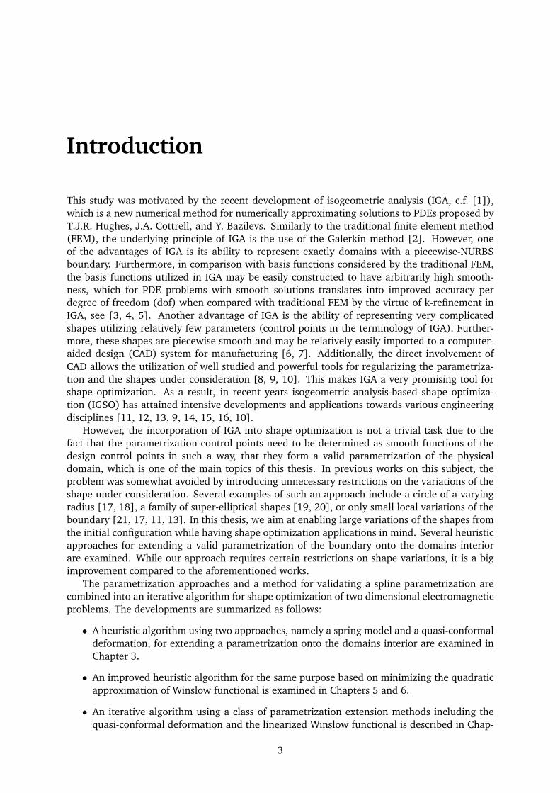
This study was motivated by the recent development of isogeometric analysis (IGA, c.f. [1]),which is a new numerical method for numerically approximating solutions to PDEs proposed byT.J.R. Hughes, J.A. Cottrell, and Y. Bazilevs. Similarly to the traditional finite element method(FEM), the underlying principle of IGA is the use of the Galerkin method [2]. However, oneof the advantages of IGA is its ability to represent exactly domains with a piecewise-NURBSboundary. Furthermore, in comparison with basis functions considered by the traditional FEM,the basis functions utilized in IGA may be easily constructed to have arbitrarily high smooth-ness, which for PDE problems with smooth solutions translates into improved accuracy perdegree of freedom (dof) when compared with traditional FEM by the virtue of k-refinement inIGA, see [3, 4, 5]. Another advantage of IGA is the ability of representing very complicatedshapes utilizing relatively few parameters (control points in the terminology of IGA). Further-more, these shapes are piecewise smooth and may be relatively easily imported to a computer-aided design (CAD) system for manufacturing [6, 7]. Additionally, the direct involvement ofCAD allows the utilization of well studied and powerful tools for regularizing the parametriza-tion and the shapes under consideration [8, 9, 10]. This makes IGA a very promising tool forshape optimization. As a result, in recent years isogeometric analysis-based shape optimiza-tion (IGSO) has attained intensive developments and applications towards various engineeringdisciplines [11, 12, 13, 9, 14, 15, 16, 10].
However, the incorporation of IGA into shape optimization is not a trivial task due to thefact that the parametrization control points need to be determined as smooth functions of thedesign control points in such a way, that they form a valid parametrization of the physicaldomain, which is one of the main topics of this thesis. In previous works on this subject, theproblem was somewhat avoided by introducing unnecessary restrictions on the variations of theshape under consideration. Several examples of such an approach include a circle of a varyingradius [17, 18], a family of super-elliptical shapes [19, 20], or only small local variations of theboundary [21, 17, 11, 13]. In this thesis, we aim at enabling large variations of the shapes fromthe initial configuration while having shape optimization applications in mind. Several heuristicapproaches for extending a valid parametrization of the boundary onto the domains interiorare examined. While our approach requires certain restrictions on shape variations, it is a bigimprovement compared to the aforementioned works.
The parametrization approaches and a method for validating a spline parametrization arecombined into an iterative algorithm for shape optimization of two dimensional electromagneticproblems. The developments are summarized as follows:
• A heuristic algorithm using two approaches, namely a spring model and a quasi-conformaldeformation, for extending a parametrization onto the domains interior are examined inChapter 3.
• An improved heuristic algorithm for the same purpose based on minimizing the quadraticapproximation of Winslow functional is examined in Chapters 5 and 6.
• An iterative algorithm using a class of parametrization extension methods including thequasi-conformal deformation and the linearized Winslow functional is described in Chap-
3
4 Preface
ters 2 and 7. We recommend interested readers to use this algorithm if they are to choosebetween the listed options.
Structure of the thesis
This thesis is organized as follows
• Part I: In this part we present the necessary mathematical background for the rest of thethesis. In Chapter 1 we recall some important properties of spline curves that are oftenutilized in the thesis. In Chapter 2, we outline our shape optimization algorithm.
• Part II: In this part we consider a model problem of shape optimization of vibrating mem-branes using IGA. On this model problem, we examine two numerical methods, a springmodel and a quasi-conformal deformation, for extending a parametrization onto the do-mains interior. The examination is presented in Chapter 3. Some issues arising from theneed for dealing with double eigenvalues are discussed in Chapter 4.
• Part III: In this part we consider the problem of designing the shapes of electromagneticantennas toward different engineering applications, from micro-antennas for energy con-centration presented in Chapter 5 to nano-antennas for field enhancement presented inChapter 6. In this part we also experiment with the use of a heuristic algorithm for shapeoptimization using IGA.
• Part IV: In this part we improve the efficiency of a device called a magnetic density sepa-rator. The IGA-based modeling of the device and an improved algorithm for performingshape optimization on the problem are presented in Chapter 7.
Part I
Isogeometric analysis and shapeoptimization
5

Chapter 1
Isogeometric analysis
Isogeometric analysis (IGA) has been recently introduced by Hughes et al. [6] and has alreadyfound many applications in a variety of engineering disciplines [7]. The original paper of IGA [6]and the textbook [7] are the recommended materials for readers who would like to study IGA.In this chapter, we rather focus on utilization of B-splines for IGA. To this end, let us first recallthe concept of B-splines and their basic properties.
1.1 B-splines
In this section, we define B-splines via a recursive formula, which requires no advanced knowl-edge and is straightforward to implement. For further properties of B-splines, we recall polarforms of polynomials. The notation used in this section, e.g., p for the degree of a B-spline,n+ p+ 1 for the number of knots in a knot vector, is borrowed from [6, 7]; in our experience, itsimplifies the indexing process in the implementation of IGA. The main reference for the sectionis [22]; see also [23, 24].
1.1.1 Definition and basis properties
Definition 1. A sequence of real numbers Ξ = t1, . . . , tn+p+1 is called a knot vector if itselements form a monotonically non-decreasing sequence
t1 ≤ . . . ≤ tp+1 < tp+2 ≤ . . . ≤ tn < tn+1 ≤ . . . ≤ tn+p+1.
Each element of the knot vector is called a knot. A knot tr is said to have multiplicity ν iftr−1 < tr = . . . = tr+ν−1 < tr+ν .
Definition 2. B-splines of degree p with the knot vector Ξ = t1, . . . , tn+p+1 are the functionsNp
1 , . . . , Npn defined recursively as follows: for i = 1, . . . , n+ p we put
N0i (t) =
1 if t ∈ [ti, ti+1[,
0 otherwise,(1.1)
and for 1 ≤ k ≤ p, i = 1, . . . , n+ p− k
Nki (t) =
t− titi+k − ti
Nk−1i (t) +
ti+k+1 − tti+k+1 − ti+1
Nk−1i+1 (t), t ∈ [ti, ti+1[. (1.2)
Definition 3. Let Np1 , . . . , N
pn be the B-splines with a knot vector Ξ = t1, . . . , tn+p+1. Further,
let c1, . . . , cn be points in Rd. The following parametrized curve
r : [tp+1, tn+1] 3 t 7→ c1Np1 (t) + . . . cnN
pn(t) ∈ Rd
is called a spline curve with control points c1, . . . , cn.
7
8 Isogeometric analysis
Remark 1. It is straightforward from (1.2) that
(i) B-splines are piecewise polynomials of degree p.
(ii) B-splines are non-negative.
(iii) B-splines are compactly supported. To be precise, the support of Npi is [ti, ti+p+2], i =
1, . . . , n. Consequently, for p + 1 ≤ r ≤ n, only the B-splines Npr−p, . . . , N
pr are supported
on [tr, tr+1].
To present further important properties of B-splines, let us first derive the fundamental de Boor’salgorithm. Let r(t) = c1N
p1 (t) + . . . cnN
pn(t) be a spline curve, with t ∈ [tr, tr+1], p + 1 ≤ r ≤ n.
Utilizing Remark 1(iii) and Equation (1.2) we have the following equalities
r(t) =r∑
i=r−pciN
pi (t) (1.3)
=
r∑
i=r−p+1
((1− t− ti
ti+p − ti
)ci−1 +
t− titi+p − ti
ci
)Np−1i (t) =
r∑
i=r−p+1
c(1)i Np−1
i (t)
= . . .
=r∑
i=r−p+k
((1− t− ti
ti+p−k+1 − ti
)c
(k−1)i−1 +
t− titi+p−k+1 − ti
c(k−1)i
)Np−ki (t) =
r∑
i=r−p+kc
(k)i Np−k
i (t)
= . . .
= c(p)r N0
r (t) = c(p)r . (1.4)
In (1.4), the intermediate control points c(k)i are given by
c(0)i = ci, i = r − p, . . . , r (1.5a)
c(k)i = (1− α(k)
i )c(k−1)i−1 + α
(k)i c
(k−1)i , r = 1, . . . , p, i = r − p− r, . . . , r, (1.5b)
where α(k)i = t−ti
ti+p−k+1−ti . Note that 1 − α(k)i and α
(k)i are barycentric coordinates of t in the
interval [ti, ti+p−k+1], i.e., t = (1−α(k)i )ti+α
(k)i ti+p−k+1. By (1.5), we have derived the de Boor’s
algorithm.
Remark 2. With the help of de Boor algorithm (1.5), we can now prove other important proper-ties of B-splines:
(i) The point r(t) with t ∈ [tr, tr+1], p + 1 ≤ r ≤ n, always belongs to the convex hull of thecontrol points cr−p, . . . , cr, and consequently a spline curve is completely contained in theconvex hull of its control points. This is due to the fact that in the kth step of de Boor’salgorithm (1.5), a new control point c
(k)i is a convex combination of the control points
c(k−1)i from the previous step.
(ii) Letting all control points in the de Boor’s algorithm (1.5) equal to 1, it follows that theB-splines form a partition of unity. That is
N1(t) + . . .+Nn(t) = 1, for all t ∈ [tp+1, tn+1[.
Note that if the knot tn+1 of the knot vector Ξ has multiplicity p + 1 then it is straight-forward from Definition 2 that all the B-splines Np
i vanish at the knot. An example is thecase where Ξ is an open knot vector, i.e., the knots tp+1 and tn+1 have multiplicity p + 1.
1.1 B-splines 9
However, this does not cause any problem for isogeometric analysis if the numerical in-tegrations under considerations are calculated using the Gaussian quadratures [25]. Thisis owing to the fact that the quadratures only require the values of the B-splines at theinteriors of knot intervals.
However, from the definition 2, it is not straightforward to explain, why a B-spline is Cp−ν at aninner knot with multiplicity ν, or what new control points are if one extra knot is inserted. Tothis end, let us invoke the following concept of polar forms.
1.1.2 Polar form of a polynomial
We shall see that each polynomial can be put into 1 : 1 correspondence with a mapping called thepolar form (also known as the blossom). This provides a powerful tool for exploring B-splines.
Definition 4. The polar form f of a polynomial F of degree p is a mapping f : Rp → R satisfyingthe following conditions
(i) f is symmetric, that is, f is invariant under any permutation of its arguments.
(ii) f is p-affine, i.e., f is affine with respect to each variable.
(iii) The restriction of f to the diagonal of Rn is F , i.e., f(t, . . . , t) = F (t).
By looking at the Taylor expansion of F (t) at a point t0 ∈ R
F (t) =
p∑
k=0
F (k)(t0)
k!(t− t0)k,
one can find a polar form of F , thereby proving the existence of the polar form, as follow
ft0(t1, . . . , tp) =
p∑
k=0
F (k)(t0)
k!
(p
k
)−1 ∑
(i1,...,ik)∈Ik
(ti1 − t0) . . . (tik − t0), (1.6)
where Ik = (i1, . . . , ik) ⊂ 1, . . . , p : i1 < . . . < ik. The uniqueness of the polar form followsfrom the following theorem
Theorem 1 (de Boor’s algorithm). Let f : Rp → R be symmetric and p-affine, and let s1 ≤. . . ≤ s2p be real numbers satisfying sp < sp+1. Then f is determined uniquely by the valuesf(si+1, . . . , si+p), i = 0, . . . , p. Furthermore, for given t1, . . . , tp, f(t1, . . . , tp) is determined by thefollowing recursive de Boor’s algorithm: for 1 ≤ k ≤ p and k ≤ i ≤ p
f(t1, . . . , tk, si+1, . . . , si+p−k) = (1− α(k)i )f(t1, . . . , tk−1, si, . . . , si+p−k)
+α(k)i f(t1, . . . , tk−1, si+1, . . . , si+p−k+1), (1.7)
where α(k)i = tk−si
si+p−k+1−si .
Proof. For each 1 ≤ k ≤ p, (1.7) is obtained by utilizing the hypothesis for f and using theexpression tk = (1− α(k)
i )si + α(k)i si+p−k+1. In the recursive formula (1.7), if we let k run from
1 to p, we end up with f(t1, . . . , tp).
We will now address the relations of the degree of continuity at a joint point between twopolynomials to their polar forms.
Theorem 2. Given two polynomials f and g of degree p, let F and G be their polar forms. Thenfor t ∈ R and r ∈ N0, the following two statements are equivalent
10 Isogeometric analysis
(i) F (k)(t) = G(k)(t), k = 0, . . . , r.
(ii) f(t, . . . , t, t1, . . . , tr) = g(t, . . . , t, t1, . . . , tr), for all t1, . . . , tr ∈ R.
Proof. Applying the chain rule to the Taylor expansion-based polar form (1.6), we arrive at theequality
F ′(t) =p
b− a(f(t, . . . , t, b)− f(t, . . . , t, a)
), (1.8)
where a 6= b are arbitrary real numbers. Differentiating both sides of (1.8) k − 1 times withrespect to t results in the following equality
F (k)(t) =k∑
i=0
Ci(p, k, a, b)f(t, . . . , t, t1, . . . , tk), (1.9)
where t1, . . . , tk ∈ a, b and Ci(p, k, a, b) are coefficients which only depend on p, k, a, and b.The equation (1.9) clearly still holds if F and f are substituted by G and g respectively, andtherefore the theorem is proven.
We are now ready to explain afore mentioned properties of B-splines.
1.1.3 B-splines in terms of polar forms and their further properties
The following theorem provides a powerful tool for establishing further properties of B-splines.
Theorem 3 (Alternative definition for B-splines). Let r(t) be a spline curve with knot vectorΞ = t1, . . . , tn+p+1 and control points c1, . . . , cn. On each knot span [tr, tr+1] with tr < tr+1, letfr be the symmetric and p-affine mapping defined by assigning its values to each of the p+ 1 sets ofp consecutive knots in the sequence of 2p knots tr−p+1, . . . , tr, tr+1, . . . , tn+r as follows
fr(tr−p+i, . . . , tr−1+i) = cr−p+i−1, i = 1, . . . , p+ 1. (1.10)
Then in [tr, tr+1], fr is the polar form of r. That is
r(t) = fr(t, . . . , t) for all t ∈ [tr, tr+1]. (1.11)
Proof. If we put
c(0)i = ci, i = r − p, . . . , r
c(k)i = fr(t, . . . , t︸ ︷︷ ︸
k times
, ti+1, . . . , ti+p−k), k = 1, . . . , p, i = k, . . . , p,
then the de Boor’s algorithm given by (1.7) gives the same relations of the intermediate controlpoints c
(k)i as given in (1.5). The former results in the right-hand side of (1.11), while the later
leads to the left-hand side of (1.11).
Remark 3. As a consequence of Theorem 3, each B-spline Npi , i = 1, . . . , n, can be defined in
terms of polar forms by using the set of control points cj = δij , j = 1, . . . , n.
We will now present one of the most important properties of B-splines.
Corollary 1. Let tr be an inner knot, i.e., p+ 2 ≤ r ≤ n, with multiplicity ν. Then any spline curveof degree p is Cn−ν at tr.
1.1 B-splines 11
Proof. Assume thattr−ν < t = tr−ν+1 = . . . = tr < tr+1.
If we let fr−ν and fr be polar forms of the spline curve in the intervals [tr−ν , t] and [t, tr+1]respectively, then fr−ν and fr have the same values at every sets of p consecutive knots of the 2p-knot sequence tr−p+1, . . . , tr−ν , t, . . . , t, tr+1, . . . , tr−ν+p. That is, at every set of p consecutiveknots containing i knots in front of t = tr−ν+1 and containing p − ν − i knots after t = tr,i = 0, . . . , p− ν, fr−ν and fr satisfy the following equalities
fr−ν(tr−ν−i+1, . . . , tr−ν , t, . . . , t,tr+1, . . . , tr+p−ν−i) =
fr(tr−ν−i+1, . . . , tr−ν , t, . . . , t, tr+1, . . . , tr+p−ν−i). (1.12)
If we put
gr−ν(s1, . . . , sp−ν) = fr−ν(t, . . . , t, s1, . . . , sp−ν) (1.13)
gr(s1, . . . , sp−ν) = fr(t, . . . , t, s1, . . . , sp−ν), (1.14)
for s1, . . . , sp−ν ∈ R, then gr−ν and gr are symmetric and (p − ν)-affine. By Theorem 1, gr−νand gr are uniquely determined by their values at all sets of p − ν consecutive knots of the settr−ν+1, . . . , tr−ν , tr+1, . . . , tr+p. Therefore, the equalities given by (1.12) ensure that gr−ν =gr. That is
fr−ν(t, . . . , t, s1, . . . , sp−ν) = fr(t, . . . , t, s1, . . . , sp−ν), for all s1, . . . , sp−ν ∈ R.
By Theorem 2, we conclude that the spline curve is Cn−ν at t = tr.
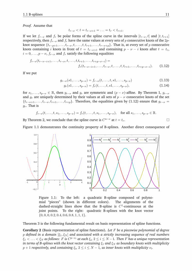
Figure 1.1 demonstrates the continuity property of B-splines. Another direct consequence of
0 0.2 0.4 0.6 0.8 10
0.1
0.2
0.3
0.4
0.5
0.6
0.7
0.8
0.9
1
N21
N22
N23
N24
N25
N26
N27
Figure 1.1: To the left: a quadratic B-spline composed of polyno-mial “pieces” (shown in different colors). The alignments of thedashed-straight lines show that the B-spline is C1-continuous at thejoint points. To the right: quadratic B-splines with the knot vector0, 0, 0, 0.2, 0.4, 0.6, 0.8, 1, 1, 1.
Theorem 3 is the following fundamental result on basis representation of spline functions.
Corollary 2 (Basis representation of spline functions). Let F be a piecewise polynomial of degreep defined in a domain [ξ1, ξN ] and associated with a strictly increasing sequence of real numbersξ1 < . . . < ξN as follows: F is Cp−νi at each ξi, 2 ≤ i ≤ N−1. Then F has a unique representationin terms of B-splines with the knot vector containing ξ1 and ξN as boundary knots with multiplicityp+ 1 respectively, and containing ξi, 2 ≤ i ≤ N − 1, as inner knots with multiplicity νi.
12 Isogeometric analysis
With the help of polar forms, it is now easy to derive the knot insertion rule.
Corollary 3 (Knot insertion). Let c1, . . . , cn be the control points of a spline curve of degree p withknot vector Ξ = t1, . . . , tn+p+1. If one extra knot t∗ ∈ [tr, tr+1], with tp+1 ≤ tr < tr+1 ≤ tn+1,is inserted to the knot sequence then the spline curve with the new knot vector is represented by thefollowing new control points
c∗i =
ci i = 1, . . . , r − p (1.15)
(1− αi)ci−1 + αici i = r − p+ 1, . . . , r (1.16)
ci−1 i = r + 1, . . . , n+ 1, (1.17)
where αi =t∗ − titi+p − ti
.
Proof. As only B-splines Npr−p, . . . , N
pr are supported on [tr, tr+1], all the control points except
cr−p, . . . , cr are unchanged. Furthermore, cr−p and cr are associated to the sets of p consecutiveknots tr−p+1, . . . , tr and tr+1, . . . , tr+p, respectively. The sets of knots are not affected by theknot insertion, thus cr−b and cr are unchanged as well. Therefore, (1.15) and (1.17) hold. Itnow remains (1.16) to be determined.
Let fr be the polar form of the spline curve defined in the interval [tr, tr+1]. For each set of pconsecutive knots containing i knots in front of t∗ and p− i− 1 knots after t∗, 0 ≤ i ≤ p− 1,
c∗r−i = fr(tr−i+1, . . . , tr, t∗, tr+1, . . . , tr+p−i−1). (1.18)
Expressing t∗ = (1− αr−i)tr−i + αr−itr+p−i, where αr−i = t∗−tr−itr+p−i−tr−i , and utilizing the p-affine
and symmetric property of fr, (1.18) becomes
c∗r−i = (1− αr−i)cr−i−1 + αr−icr−i, 0 ≤ i ≤ p− 1. (1.19)
Substituting r − i by i in (1.19), we reach the conclusion (1.16), thereby completing the proof.
Finally, let us discuss the B-spline representation of the derivative of a spline curve.
Corollary 4 (Derivative of B-splines). Let r be a spline curve of degree p with knot vector Ξ =t1, . . . , tn+p+1 and control points c1, . . . , cn. Then the derivative r′ is a spline curve of degreep− 1 with the same knot vector and the following control points
c′i =p
ti+p − ti(ci − ci−1), i = 1, . . . , n+ 1. (1.20)
Consequently, the derivatives of B-splines are given by
d
dtNpi =
p
ti+p − tiNp−1i − p
ti+p+1 − ti+1Np−1i+1 , i = 1, . . . , n. (1.21a)
Proof. By Corollary 2, r′ is a spline curve of degree p − 1 with, for convenience, the same knotvector Ξ. Let us now determine the control points c′i, 1 ≤ i ≤ n− 1. Let fr be the polar form ofr in the interval [tr, tr+1], where r satisfies i + 1 ≤ r ≤ i + p. From the Taylor expansion-basedrepresentation of a polar form (1.6), it follows that the polar form gr of r′ in [tr, tr+1] is given by
gr(ξ1, . . . , ξp−1) =p
b− a(fr(ξ1, . . . , ξp−1, b)− fr(ξ1, . . . , ξp−1, a)
), (1.22)
for all ξ1, . . . , ξp−1 ∈ R and real numbers a 6= b. Substituting (ξ1, . . . , ξp−1) = (ti+1, . . . , ti+p−1),b = ti+p, and a = ti to (1.22), we arrive at the conclusion (1.20).
For each 1 ≤ i ≤ n, applying (1.20) to the set of control points ck = δik, k = 1, . . . , n, (1.21)is established.
1.2 Isogeometric analysis 13
1.2 Isogeometric analysis
In this section, we first state IGA precisely. Enforcement of C0-continuity of the numericalsolution when using a model with multiple IGA patches is then discussed.
1.2.1 Isogeometric analysis: Basis functions for analysis
Let us again consider a simply connected open domain Ω ⊂ R2. We are looking for a B-splineparametrization of Ω, that is, for a bijective map F : [0, 1]2 → Ω of the form
F(u, v) =(x(u, v), y(u, v)
)=
m∑
i=1
n∑
j=1
di,jMpi (u)N q
j (v), (1.23)
where Mpi and N q
i are B-splines of degree p and q with knot vectors Ξu and Ξv, respectively.By composing the inverse F−1 with some basis functions on the parameter (reference) domain]0, 1[2 we obtain basis functions defined on the physical domain Ω.
We let M pi , i = 1, . . . , m and N q
j , j = 1, . . . , n be B-splines of degree p and q (not necessary
equal to p and q) with knot vector Ξu and Ξv, respectively. The basis functions on the parameterdomain are defined as the tensor product splines
Rp,qk (u, v) = M pi (u)N q
j (v), k = (n− 1)i+ j. (1.24)
Thus, the basis functions on the physical domain Ω are given as
φk(x, y) = (Rp,qk F−1)(x, y), k = 1, . . . , mn. (1.25)
An integral over Ω can be now transformed to an integral over ]0, 1[2 as∫∫
Ω
f(x, y) dx dy =
∫∫
]0,1[2
f(x(u, v), y(u, v)) det(J) dudv, (1.26)
where J is the Jacobian of the variable transformation F, and we have assumed that det(J) > 0.Furthermore, to ensure that we can approximate any function in H1(Ω) [26] sufficiently
well, we may want to use an even finer (when compared to Ξu and Ξv) pair of knot vectors Ξu
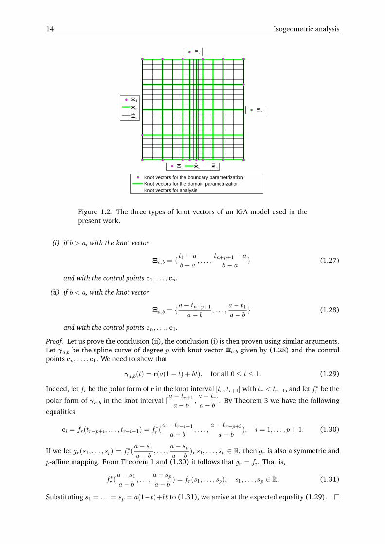
and Ξv for the analysis, see Fig. 1.2.
Remark 4. As a consequence of the formula (1.26), one may evaluate integrals over Ω enteringa variational form of a given boundary value problem by computing the integrals over the pa-rameter domain instead. Thus an “IGA assembly routine” may be implemented as a loop overelements defined by the knot vectors Ξu and Ξv, see Fig. 1.2.
1.2.2 Multiple patches: Enforcement of the C0-continuity of the numerical solu-tion
1.2.2.1 Theory
Often, it is convenient or even necessary to consider domains subdivided into several patches.Examples include non-simply connected domains or physical models involving several materials.For enforcing the C0-continuity of the numerical solution across patch boundaries, we need thefollowing property of spline curves.
Lemma 1. Let r be a spline curve of degree p with knot vector Ξ = t1, . . . , tn+p+1 and controlpoints c1, . . . , cn. Then the following curve
[0, 1] 3 t 7→ r(a(1− t) + bt) ∈ Rd, tp+1 ≤ a 6= b ≤ tn+1,
is a spline curve,
14 Isogeometric analysis
Ξ1 Ξu Ξu
Ξ3
Ξ2
Ξ4
Ξv
Ξv
Knot vectors for the boundary parametrizationKnot vectors for the domain parametrizationKnot vectors for analysis
Figure 1.2: The three types of knot vectors of an IGA model used in thepresent work.
(i) if b > a, with the knot vector
Ξa,b = t1 − ab− a , . . . ,
tn+p+1 − ab− a (1.27)
and with the control points c1, . . . , cn.
(ii) if b < a, with the knot vector
Ξa,b = a− tn+p+1
a− b , . . . ,a− t1a− b (1.28)
and with the control points cn, . . . , c1.
Proof. Let us prove the conclusion (ii), the conclusion (i) is then proven using similar arguments.Let γa,b be the spline curve of degree p with knot vector Ξa,b given by (1.28) and the controlpoints cn, . . . , c1. We need to show that
γa,b(t) = r(a(1− t) + bt), for all 0 ≤ t ≤ 1. (1.29)
Indeed, let fr be the polar form of r in the knot interval [tr, tr+1] with tr < tr+1, and let f∗r be the
polar form of γa,b in the knot interval [a− tr+1
a− b ,a− tra− b ]. By Theorem 3 we have the following
equalities
ci = fr(tr−p+i, . . . , tr+i−1) = f∗r (a− tr+i−1
a− b , . . . ,a− tr−p+ia− b ), i = 1, . . . , p+ 1. (1.30)
If we let gr(s1, . . . , sp) = f∗r (a− s1
a− b , . . . ,a− spa− b ), s1, . . . , sp ∈ R, then gr is also a symmetric and
p-affine mapping. From Theorem 1 and (1.30) it follows that gr = fr. That is,
f∗r (a− s1
a− b , . . . ,a− spa− b ) = fr(s1, . . . , sp), s1, . . . , sp ∈ R. (1.31)
Substituting s1 = . . . = sp = a(1−t)+bt to (1.31), we arrive at the expected equality (1.29).
1.2 Isogeometric analysis 15
The C0-continuity of the numerical solution across boundaries between patches can be en-forced as follows
• We parametrize all patches in the counter-clockwise fashion, i.e., a valid parametrizationof this type has positive Jacobian determinant everywhere.
• At a boundary Γ between two patches, let spline curves ri with knot vectors Ξi = t(i)1 , . . . ,
t(i)ni+p+1 and control points ci1, . . . , c
ini , i = 1, 2, be the induced parametrizations of the
two parametrizations of the two patches of Γ, respectively. According to the direction ofincreasing parameter of the induced parametrizations, there are two cases, see Fig. 7.6 forillustrations,
(i) r′1(t) · r′2(t) > 0 for all 0 < t < 1, i.e., r1 and r2 have co-directional tangent vectors.The criteria for the numerical solution to be continuous across Γ are1. The two parametrizations are continuous across Γ, i.e., r1(t) = r2(t) for all t ∈
F−1i(Γ). This criterion is formulated as follows. First we find the “union” knot
vector Ξ of Ξ1 and Ξ2, i.e., the knot vector whose inner knots are all innerknots of both knot vectors with maximum multiplicity. Let Ri be the refinementmatrices [24] obtained when inserting knots into Ξi to have Ξ, i = 1, 2. The C0-continuity of the parametrizations now can be enforced by the following linearconstraints on the control points
R1[x11, . . . , x
1n1
]T = R2[x21, . . . , x
2n2
]T , (1.32)
where xij is one of the coordinates of the control points cij .2. The same conditions as in (1.32) are enforced for the state variables, i.e., the
coefficients of the representation of the numerical solution in terms of the basisfunctions given by (1.25).
(ii) r′1(t) · r′2(t) < 0 for all 0 < t < 1, i.e., the tangent vectors of r1 and r2 are the vectorswith opposite directions. The criteria for the numerical solution to be continuousacross Γ are1. The two parametrizations are “continuous” across Γ, i.e., r1(1 − t) = r2(t) for all
t ∈ F−1i (Γ). This criterion is formulated as follows. Applying Lemma 1 with a = 1
and b = 0 for r1 to get the new knot vector Ξ1,1,0 = 1 − t(1)ni+p+1, . . . , 1 − t
(1)1 .
Then similar to the previous case, we find the “union” knot vector Ξ of Ξ1,1,0
and Ξ2. Let R1 and R2 be the refinement matrices obtained when insertingknots into Ξ1,1,0 and Ξi to have Ξ, respectively. The linear constraints for the“C0-continuity” of the parametrizations are
R1[x1n1, . . . , x1
1]T = R2[x21, . . . , x
2n2
]T , (1.33)
where xij is one of the coordinates of the control points cij .2. The same conditions as in (1.33) are enforced for the state variables.
• Let Ch = c be the constraints, discussed above, on state variables h. Let Kh = f bethe global discretization of the linear system, resulting from assembling matrices from allpatches. Then h can be determined via the stationary point of the following Lagrangefunction with Lagrange multipliers λ [27]
Λ(h,λ) =1
2hTKh− hT f + λT (Ch− c). (1.34)
That is, [K CT
C 0
] [hλ
]=
[fc
]. (1.35)
16 Isogeometric analysis
∂F2
∂uF3
∂F3
∂u
∂F2
∂v
∂F1
∂u
∂F1
∂v
∂F3
∂v
F2
24
3
face edge
1
2
34
F1 ∂F2
∂u · ∂F3
∂v < 0
1
∂F1
∂v · ∂F2
∂v > 0
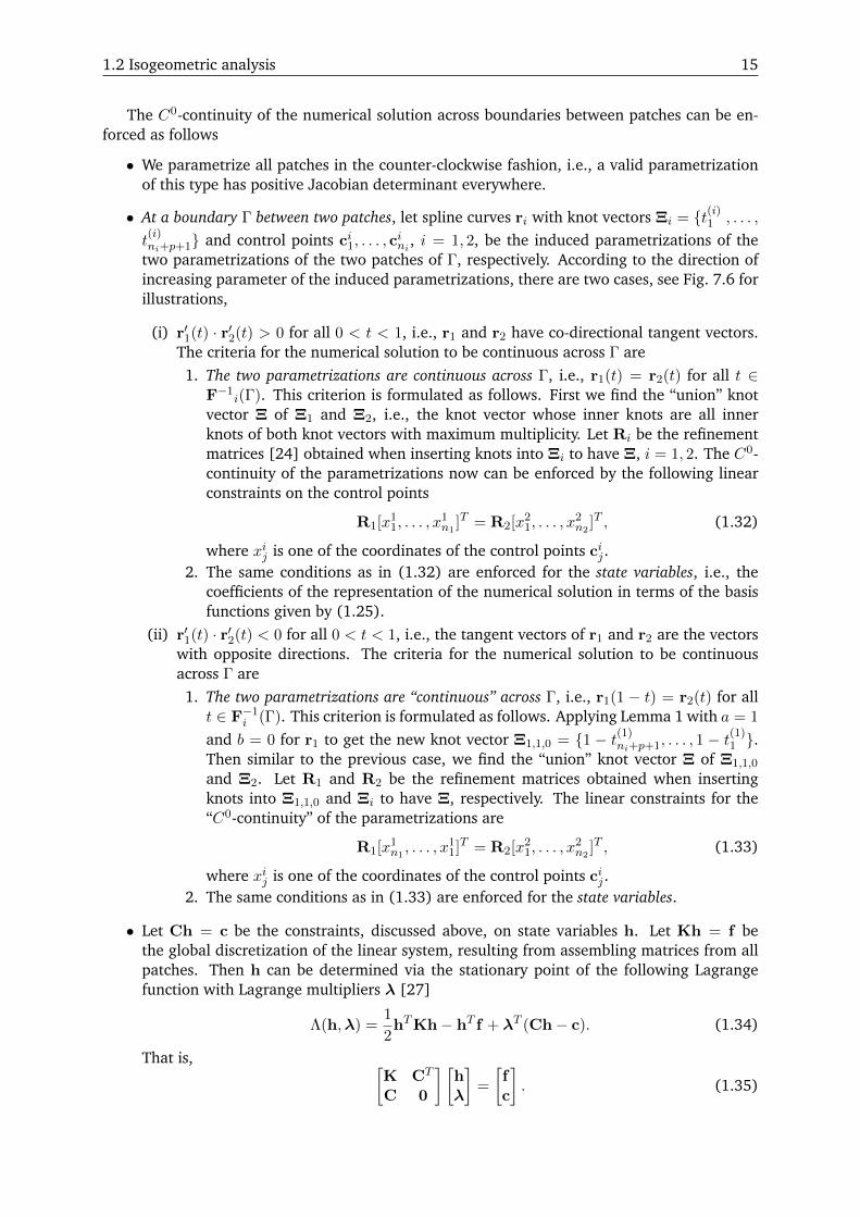
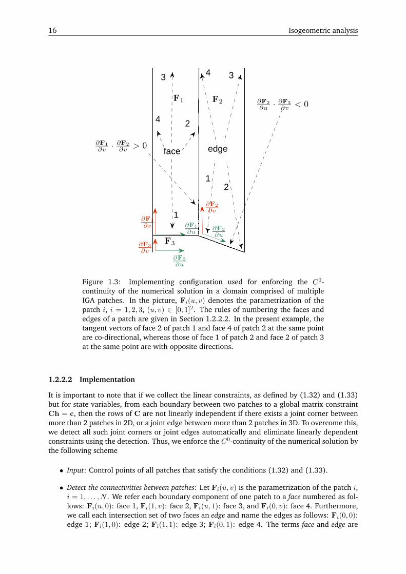
Figure 1.3: Implementing configuration used for enforcing the C0-continuity of the numerical solution in a domain comprised of multipleIGA patches. In the picture, Fi(u, v) denotes the parametrization of thepatch i, i = 1, 2, 3, (u, v) ∈ [0, 1]2. The rules of numbering the faces andedges of a patch are given in Section 1.2.2.2. In the present example, thetangent vectors of face 2 of patch 1 and face 4 of patch 2 at the same pointare co-directional, whereas those of face 1 of patch 2 and face 2 of patch 3at the same point are with opposite directions.
1.2.2.2 Implementation
It is important to note that if we collect the linear constraints, as defined by (1.32) and (1.33)but for state variables, from each boundary between two patches to a global matrix constraintCh = c, then the rows of C are not linearly independent if there exists a joint corner betweenmore than 2 patches in 2D, or a joint edge between more than 2 patches in 3D. To overcome this,we detect all such joint corners or joint edges automatically and eliminate linearly dependentconstraints using the detection. Thus, we enforce the C0-continuity of the numerical solution bythe following scheme
• Input: Control points of all patches that satisfy the conditions (1.32) and (1.33).
• Detect the connectivities between patches: Let Fi(u, v) is the parametrization of the patch i,i = 1, . . . , N . We refer each boundary component of one patch to a face numbered as fol-lows: Fi(u, 0): face 1, Fi(1, v): face 2, Fi(u, 1): face 3, and Fi(0, v): face 4. Furthermore,we call each intersection set of two faces an edge and name the edges as follows: Fi(0, 0):edge 1; Fi(1, 0): edge 2; Fi(1, 1): edge 3; Fi(0, 1): edge 4. The terms face and edge are
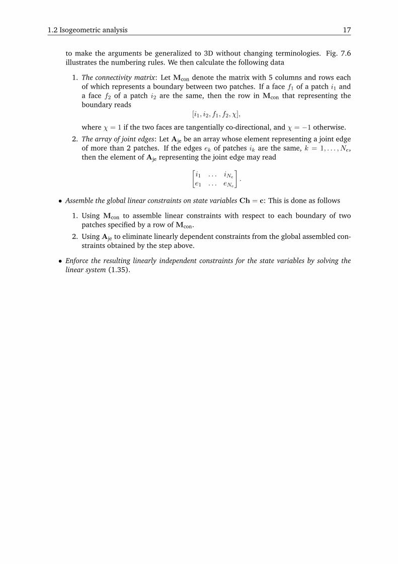
1.2 Isogeometric analysis 17
to make the arguments be generalized to 3D without changing terminologies. Fig. 7.6illustrates the numbering rules. We then calculate the following data
1. The connectivity matrix: Let Mcon denote the matrix with 5 columns and rows eachof which represents a boundary between two patches. If a face f1 of a patch i1 anda face f2 of a patch i2 are the same, then the row in Mcon that representing theboundary reads
[i1, i2, f1, f2, χ],
where χ = 1 if the two faces are tangentially co-directional, and χ = −1 otherwise.
2. The array of joint edges: Let Aje be an array whose element representing a joint edgeof more than 2 patches. If the edges ek of patches ik are the same, k = 1, . . . , Ne,then the element of Aje representing the joint edge may read
[i1 . . . iNee1 . . . eNe
].
• Assemble the global linear constraints on state variables Ch = c: This is done as follows
1. Using Mcon to assemble linear constraints with respect to each boundary of twopatches specified by a row of Mcon.
2. Using Aje to eliminate linearly dependent constraints from the global assembled con-straints obtained by the step above.
• Enforce the resulting linearly independent constraints for the state variables by solving thelinear system (1.35).

Chapter 2
Shape optimization using isogeometricanalysis
In this chapter, we first describe techniques for handling spline parametrizations. We thenpresent an iterative algorithm for incorporating isogeometric analysis into shape optimizationthat has been tested with the design problem of magnetic density separators in Chapter 7 andwith the antenna design problem in Part III. A parametrization setting and sensitivity analysisfor a general shape optimization problem are described afterwards.
2.1 B-spline parametrization
In this section, we recall techniques for handling B-spline parametrizations in isogeometric anal-ysis while having their utilizations for shape optimization in mind. For more details, see [28,29, 30, 10].
2.1.1 Jacobian determinant of a parametrization as a spline
In order to ensure the validity of a parametrization of Ω when some of the control points di,j , i =1, . . . , n, j = 1, . . . , m are design variables, we employ the following approach. The determinantof the Jacobian of F given by (1.23) is computed as
det(J) =
m,n∑
i,j=1
m,n∑
k,`=1
det[di,j , dk,`]dMp
i (u)
duN qj (v) Mp
k (u)dN q
` (v)
dv, (2.1)
where det[di,j , dk,`] is the determinant of the 2×2 matrix with columns di,j , dk,`. Equation (2.1)defines a piecewise polynomial of degree 2p − 1 in u and degree 2q − 1 in v, with the differen-tiability at a knot lower by 1 in u and also lower by 1 in v. Such a map can be written in termsof B-splinesM2p−1
k and N 2q−1` of degree 2p− 1 and 2q − 1 with the knot vectors obtained from
Ξu and Ξv by raising the multiplicities of the inner u-knots and v-knots by p and q, respectively.That is
det(J) =
M,N∑
k,`=1
ck,`M2p−1k (u)N 2q−1
` (v). (2.2)
As B-splines are non-negative, the positivity of the determinant can be ensured by the positivityof the coefficients ck,`. Let (N 2q−1
` )∗ be a function having the following form
(N 2q−1` )∗ = α1N 2q−1
1 + . . . αNN 2q−1N , (2.3)
19
20 Shape optimization using isogeometric analysis
and satisfying the conditions
〈(N 2q−1` )∗,N 2q−1
j 〉 =
N∑
i=1
αk
∫ 1
0N 2q−1i (v)N 2q−1
j (v) dv = δ`,j , j = 1, . . . , N. (2.4)
(N 2q−1` )∗ is called the dual functional of N 2q−1
` , and may be determined by solving the systemof linear equations (2.4) for unknowns α1, . . . , αN . Utilizing the fact that (M2p−1
k N 2q−1` )∗ =
(M2p−1k )∗(N 2q−1
` )∗, and substituting (2.1) to the relation ck,` = 〈(M2p−1k N 2q−1
` )∗, det(J)〉 wearrive at the following
ck,` =
m,n∑
i,j=1
m,n∑
α,β=1
det[di,j , dα,β] 〈 (M2p−1k )∗ ,
dMpi
duMpα 〉 〈 (N 2q−1
` )∗ , N qj
dN qβ
dv〉. (2.5)
If we let d denote the vector containing coordinates of the control points di,j , then (2.5) showsthat ck,` are quadratic forms of d. The equation (2.5) also specifies coefficients of the matrices,denoted by Qk,`, of the quadratic forms. Thus we can write
ck,` = dTQk,`d. (2.6)
We now look for a linear method for extending a spline parametrization of the boundary ofthe physical domain onto the domain interior. By the term linear, we mean that that the resultinginner control points from the method are affine mappings of boundary control points. The linearmethod used in this work does not only depend on the knot vectors for the domain parametriza-tion Ξu and Ξv but also depends on a reference parametrization of the domain. We obtainthe reference parametrization by a minimization problem related to a so-called the Winslowfunctional [31]. We then “linearize” the Winslow functional to obtain the linear method. Theapproach for obtaining a reference parametrization of the domain and the derivation of thelinear method are presented as follows.
2.1.2 Obtaining a B-spline parametrization
None of the linear methods presented in [29, 30] for extending the parametrization of theboundary into the interior of the domain can in general guarantee that the resulting map F willsatisfy det(J) > 0 everywhere on [0, 1]2. Therefore, during some shape optimization iterationswe have to utilize a more expensive non-linear method for improving the distribution of theinterior control points di,j . In a view of (2.2), a natural approach to ensure that det(J) isbounded away from zero is to solve the following optimization problem:
maximizedi,j ,z
z,
subject to ck,`(di,j)≥ z,
(2.7)
where di,j are inner control points as stated in (1.23), ck,` are given by (2.2), and z is an auxiliaryoptimization variable. If z resulting from approximately solving (2.7) to local optimality ispositive then we are guaranteed to have a valid parametrization. Unfortunately, the quality ofthe parametrization obtained in this fashion needs not to be very high. We can further improvethe parametrization by trying to approximate a conformal map. That is, ideally we would likeg = JTJ to be an identically diagonal matrix (e.g., see [32]).
Let λ1 and λ2 be the eigenvalues of the matrix g. Then g satisfies the ideal condition if andonly if λ1 = λ2. The identity
(√λ1 −
√λ2)2
√λ1λ2
=λ1 + λ2√λ1λ2
− 2 (2.8)
2.1 B-spline parametrization 21
initialize a control net
solve (2.7) to finda parametrization
z0 ≤ 0?
minimize Winslowfunctional, see (2.10)
If ck` ≤ 0 re-fine the supportof Mk(u)N`(v)
∃ck` < 0?
stop
yes
no
yes
no
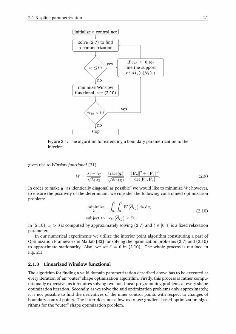
Figure 2.1: The algorithm for extending a boundary parametrization to theinterior.
gives rise to Winslow functional [31]
W =λ1 + λ2√λ1λ2
=trace(g)√
det(g)=‖Fu‖2 + ‖Fv‖2
det[Fu,Fv]. (2.9)
In order to make g “as identically diagonal as possible” we would like to minimize W ; however,to ensure the positivity of the determinant we consider the following constrained optimizationproblem:
minimizedi,j
∫ 1
0
∫ 1
0W(di,j)
dudv,
subject to ck`(di,j)≥ δz0.
(2.10)
In (2.10), z0 > 0 is computed by approximately solving (2.7) and δ ∈ [0, 1] is a fixed relaxationparameter.
In our numerical experiments we utilize the interior point algorithm constituting a part ofOptimization Framework in Matlab [33] for solving the optimization problems (2.7) and (2.10)to approximate stationarity. Also, we set δ = 0 in (2.10). The whole process is outlined inFig. 2.1.
2.1.3 Linearized Winslow functional
The algorithm for finding a valid domain parametrization described above has to be executed atevery iteration of an “outer” shape optimization algorithm. Firstly, this process is rather compu-tationally expensive, as it requires solving two non-linear programming problems at every shapeoptimization iteration. Secondly, as we solve the said optimization problems only approximately,it is not possible to find the derivatives of the inner control points with respect to changes ofboundary control points. The latter does not allow us to use gradient based optimization algo-rithms for the “outer” shape optimization problem.
22 Shape optimization using isogeometric analysis
To avoid this difficulty, we linearize the process of computing a domain parametrization.Namely, we can Taylor-expand the Winslow functional as
W(d) =
∫∫
ΩW (d) dudv ≈ W(d0) + (d− d0)T G(d0) +
1
2(d− d0)T H(d0) (d− d0), (2.11)
where d is a vector with all control points di,j , d0 is the control points for a reference parametriza-tion obtained by solving (2.10), and G and H are the gradient and Hessian of W respectively.If we split the control points d = (d1 d2)T into the part d2 that is given (typically the boundarycontrol points) and the part d1 that has to be determined (typically the inner control points),then we can write (2.11) as
W(d) ≈ W(d0) +(d1 − d1,0 d2 − d2,0
)(G1
G2
)
+1
2
(d1 − d1,0 d2 − d2,0
)(H11 H12
H21 H22
)(d1 − d1,0
d2 − d2,0
). (2.12)
The minimum of the right hand side of (2.12) is obtained when d1 satisfies the linear equation
H11(d1 − d1,0) = −G1 −H12(d2 − d2,0). (2.13)
This gives us a fast method for computing the domain parametrization and its derivatives withrespect to the boundary control points. We use this method as long as we obtain a validparametrization, but if the parametrization at some point fails the test described in Section 2.1.1then we restart the “outer” shape optimization algorithm with a new reference parametrizationd0 found by the method described in Section 2.1.2.
The given control points d2 can further be split into the set of fixed control points df andcontrol points Rd obtained from the design variables (control points) d by knot insertion (re-finement).
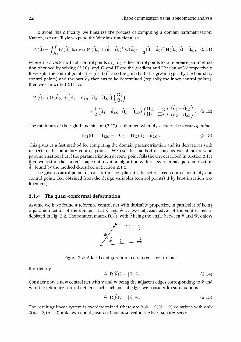
2.1.4 The quasi-conformal deformation
Assume we have found a reference control net with desirable properties, in particular of beinga parametrization of the domain. Let v and w be two adjacent edges of the control net asdepicted in Fig. 2.2. The rotation matrix R(θ), with θ being the angle between v and w, enjoys
v
wθ
Figure 2.2: A local configuration in a reference control net
the identity‖w‖R(θ)v = ‖v‖w. (2.14)
Consider now a new control net with v and w being the adjacent edges corresponding to v andw of the reference control net. For each such pair of edges we consider linear equations
‖w‖R(θ)v = ‖v‖w. (2.15)
The resulting linear system is overdetermined (there are 8(m − 2)(n − 2) equations with only2(m− 2)(n− 2) unknown nodal positions) and is solved in the least squares sense.
2.2 Shape optimization algorithm 23
2.1.5 Multiple patches
Let us discuss the case where a physical domain is configured by several patches. In any case, theparametrization of the domain boundary is given. Thus, the task of extending the parametriza-tion into the interior is the same as in the one patch case except the parametrizations of innerpatch boundaries are unknown. For such a domain, the optimization problems (2.7), (2.10),and the linear system (2.13) should account for the control points with respect to the innerboundaries as design variables while maintaining C0-continuities across the boundaries by lin-ear constraints on the control points. The constraints are obtained using the approach discussedin Section 1.2.2.1.
2.2 Shape optimization algorithm
Let us consider the following shape optimization problem using isogeometric analysis
minimized∈Ωd
f(d) (2.16)
where Ωd ⊂ Rn is the space of design variables, and d are typically coordinates of boundarycontrol points of spline patches. We solve the problem by the following iterative algorithm
• Start the algorithm with a guess d0 ∈ int(Ωd).
• Let Ad0 and Bd0 be the matrices of an affine mapping that represent an approach forextending a parametrization of the boundary of the physical domain under considerationonto the domain interior. That is, the approach results in all control points d from daccording to the following relation
d(d) = Ad0d + Bd0 , d ∈ Ωd. (2.17)
Assume Ad0 and Bd0 satisfy the condition that d(d0) = Ad0d0+Bd0 corresponds to a validparametrization. Thus with a sufficient subdivision of the Jacobian determinant surface,c.f. (2.1), its representing control points ck,` given by (2.2) are positive. For simplicity letus assume that without further subdivision, the control points ck,` are positive. Accordingto (2.6)
ck,`(d) = (Ad0d + Bd0)TQk,`(Ad0d + Bd0). (2.18)
The control points ck,` are obviously continuous functions of d, thus there exists a neigh-borhood Bd0 ⊂ Ωd0 of d0 such that
ck,`(d) > 0 ∀d ∈ Bd0 , ∀k, `. (2.19)
• We then would like to solve the following sub-optimization problem
d1 = argmind∈Bd0
f(d), (2.20)
where argmin denotes the argument of the minimum of a function. In practice, it is difficultto determine Bd0 , especially the “maximal” one, i.e., the largest neighborhood satisfying(2.19). Instead, we find d1 as the solution to the following problem
minimized∈Ωd
f(d), (2.21a)
such that ck,`(d) ≥ ε, (2.21b)
where ε is some positive constant. Note that the values and sensitivities of the constraints(2.21b) are very easy to compute using (2.18).
24 Shape optimization using isogeometric analysis
• Repeat the steps above by replacing d0 with d1, and stop when convergence.
Remark 5. We note that
(i) The linearized Winslow functional presented in Section 2.1.3 and the quasi-conformaldeformation presented in Section 2.1.4 are among the methods that fulfill the conditionrelated to (2.17).
(ii) In J. Gravesen et al. [28], any parametrization of a 2D B-spline patch with a corner havingangle more than π is invalid. Therefore, it is necessary to constrain the angles. Fortunately,they are already included in the constraints (2.21b) as those on the corner control pointsof the Jacobian determinant ensure the “validity” of the corresponding angles.
(iii) One problem of shape optimization using isogeometric analysis has been encounteredin fluid mechanics is the clustering of control points [28]. This requires some specialtreatment [28]. Interestingly, without extra efforts the algorithm above avoids this issue.Indeed, since the the boundary control points of the Jacobian determinant are constrainedto be positive, the boundary parametrization must be locally regular.
2.3 Multiple methods of extending parametrization from boundaryto interior
For some problems, there are regions which can be parametrized in a simple and effective way.For such a case, it is not necessary to employ more complicated and expensive methods to extendthe parametrization from the boundaries to the interiors of those regions. Thus in general wecan have different parametrization extension methods for different regions. See Fig. 7.10 andFig. 7.13 for illustrations of the argument.
For the sake of deriving sensitivity later on and implementation, let us formulate the gen-eral configuration. Let Ω be a connected domain. Assume that according to parametrizationextension, Ω can be partitioned into N sub-domains Ωk, k = 1, . . . , N . Each sub-domains arecomprised of several spline patches. Let d be the design variable vector and dk be the controlpoint vector of ∂Ωk. The first task for the algorithm is to determine affine maps that sending dto dk as
dk = akd + bk. (2.22)
The next task will be to derive affine transformations that map dk to unknown inner controlpoints of Ωk, and therefore to the control point vector dk of Ωk
dk = Akdk + Bk = Akakd + Akbk + Bk. (2.23)
Note that the refinement matrices [24] obtained when inserting knots into the boundary knotvectors to have parametrization knot vectors are already taken into account in Ak. If for somesub-domain Ωk, the parametrization extension method used in this domain is guaranteed toresult in a valid parametrization then the constraints (2.21b) with respect to this domain shouldbe removed to reduce computational time consume.
2.4 Sensitivity analysis
Let the governing system of linear algebraic equations for the numerical model under consider-ation be the following
Kh = f , (2.24)
where h is the vector of state variables, i.e., the coefficients of the representation of the nu-merical solution in terms of the basis functions given by (1.25). If the objective function or a
constraint of the considered shape optimization relates to an integral over a domain Ω0, thenvery often we can keep the parametrization of Ω0 fixed, i.e., independent from changes of de-sign control points, e.g., see Fig. 7.11. Thus to determine the partial derivative of a functionwith respect to a design variable di, we only need to determine ∂h
∂di. Differentiating both sides
of (2.24), the partial derivative is in turn the solution to the following linear system
K∂h
di= −∂K
dih +
∂f
di. (2.25)
In (2.25), the partial derivatives of K and f with respect to di can often be calculated straightfor-wardly. Finally, as we employ linear parametrization methods formulated in (2.23), the desiredsensitivities are
∂I
∂d= aT1 AT
1
∂I
∂d1
+ . . .+ aTNATN
∂I
∂dN. (2.26)
25

Part II
Prescription for first few eigenvalues ofthe Laplacian operator
27

Chapter 3
Isogeometric shape optimization ofvibrating membranes
Nguyen D. M., A. Evgrafov, A.R. Gersborg, J. Gravesen, Isogeometric shape optimization of vi-brating membranes, Computer Methods in Applied Mechanics and Engineering, vol. 200, pp. 1343-1353, 2011.
Abstract. We consider a model problem of isogeometric shape optimization of vibrating mem-branes whose shapes are allowed to vary freely. The main obstacle we face is the need forrobust and inexpensive extension of a spline parametrization from the boundary of a domainonto its interior, a task which has to be performed in every optimization iteration. We experi-ment with two numerical methods (one is based on the idea of constructing a quasi-conformalmapping, whereas the other is based on a spring-based mesh model) for carrying out this task,which turn out to work sufficiently well in the present situation. We perform a number of nu-merical experiments with our isogeometric shape optimization algorithm and present smooth,optimized membrane shapes. Our conclusion is that isogeometric analysis fits well with shapeoptimization.
Keywords: Isogeometric analysis, shape optimization, spline parametrization, vibrating mem-brane, eigenvalue.
3.1 Introduction
Shape optimization is a classical mathematical problem with a multitude of applications in engi-neering disciplines; see for example the monographs [34, 35] and references therein. From thetheoretical perspective, the most interesting cases occur when the shapes under considerationare not restricted to be diffeomorphic to each other, that is, when changes in the topology are al-lowed. Such problems are often treated by parametrizing the shape indirectly, using for examplethe coefficients of the partial differential equation governing an engineering model under con-sideration (control in the coefficients, homogenization, or topology optimization approaches,see [36, 37]) or auxiliary surfaces such as in level-set methods, see [38]. All the mentionedmethods gain their computational efficiency from the fact that they are based on fixed grids,which provides a tremendous advantage particularly in 3D.
Having industrial applications in mind, it would be convenient to integrate geometry opti-mization into CAD environments. For this to be possible one needs to utilize a direct CAD-likerepresentations of the boundary. Such a representation should be maintained at every opti-mization iteration by shape optimization methods at the expense of needing to re-generate or
29
to update frequently the volumetric mesh, which is needed for solving equations governing agiven system. This expense imposes a computational penalty on the total performance of shapeoptimization methods.
One promising method of combining the efficiency of the computations on a fixed grid withthe demand of a direct CAD-like parametrization of the boundary within the shape optimiza-tion framework is utilizing isogeometric analysis (IGA) for numerically solving the equationsgoverning a given engineering system [6, 39, 40, 41, 11, 18, 42, 13]. In this way one keepsall the computations on a fixed mesh on a parameter domain while gaining the advantage thatoptimized geometries can be easily processed in CAD systems for manufacturing [6, 7].
In the present paper we utilize isogeometric analysis-based shape optimization (IGSO) fordesigning vibrating membranes with prescribed eigenvalues. We treat vibrating membranes asas a model problem for more general spectral shape optimization problems of systems governedby elliptic operators [43, 44]. It is also closely related to eigenfrequency optimization problemsof vibrating plates with holes [19, 20, 45]. The problem of designing vibrating membranesis by no means a novel one: for example Hutchinson and Niordson [46] computed shapes ofdrums where the first few eigenvalues were prescribed. In particular, they considered the designproblem of a harmonic drum, namely, a membrane whose first four eigenfrequencies form a ratioof 2:3:3:4. (The reason for the double eigenvalues is that it seems impossible to design a drumwith frequencies 2:3:4 [47, 43, 48]). The idea in [46] was to use a conformal map from thecircular domain to the domain occupied by the drum and to perform the eigenfrequency analysison the former domain. Note that this idea is similar to IGA in the sense that a parametrizationof the domain is utilized. Kane and Schoenauer [49] later attacked the problem by geneticalgorithms, while in the present work we utilize gradient-based algorithms within the IGSOframework. We emphasize that we consider the problem as a model on which we can illustratevarious re-parametrization strategies within IGSO context.
In the present work, the only generic requirement we place on a family of candidate feasibleshapes in the shape optimization problems we consider is that they are diffeomorphic to eachother. Whereas this requirement may be viewed as a restrictive one from the theoretical per-spective, it is much more general than what is often considered within the shape optimizationframework and leads to certain computational challenges. This is in a stark contrast with thesituations when domain families parametrized by only a few variables are consedered (such as,for example, a circle of a varying radius [17, 18], or a family of super-elliptical shapes [19, 20]),or when only certain parts of the boundary are allowed to vary locally [21, 17, 11, 13]. Restric-tions on the variations of the shape simplify significantly the task of remeshing in a FEM-basedshape optimization, or the task of extending the parametrization from the boundary into theinterior of the domain in IGSO-based shape optimization.
Owing to the richness of the family of shapes which we allow, constructing the expensionof parametrization from the boundary into the interior of the domain becomes a non-trivialtask in the present situation. We experiment with two linear methods for computing such anextension numerically: one is based on a spring model of the mesh and the other one is basedon the idea of a quasi-conformal deformation. The former method is inspired by ideas comingfrom linear elasticity and works well for problems with convex domains. The strategy for thelatter method is to find a well-behaving spline parametrization of an initial reference shape bysolving auxiliary optimization problems, and then generate the inner control points by “quasi-conformally deforming” the reference shape into the resulting configuration. The procedure isrepeated if an invalid parametrization appears at some shape optimization iteration.
The remainder of this paper is organized as follows. In Section 2, we briefly recall theequations governing vibrating membranes and their Galerkin discretization. The IGA modelused in the present work and necessary techniques of handling a spline parametrization arepresented in Section 3. In Section 4, we state the IGSO problem formulation and its sensitivity
30
analysis. Our numerical experiments with IGSO are reported in Section 5. We conclude thepaper with a summary of the results.
3.2 Physical problem
In this section we briefly recall the partial differential equations governing harmonic oscillationsof a membrane and their Galerkin discretization.
3.2.1 Governing equation
Let Ω be a membrane whose circumference Γ is constrained to be motionless. The out-of-planedisplacement U(x, t) of a point x ∈ Ω at time t obeys the wave equation with homogeneousDirichlet boundary condition
∂2U(x, t)
∂t2= c2∆U(x, t) ∀x ∈ Ω (3.1)
U(x, t) = 0 ∀x ∈ Γ (3.2)
where ∆ is the spatial Laplacian operator and c is the wave speed, depending on the tensionand the surface density of the membrane (c.f. [50]). Without losing generality, in what followswe assume that c = 1.
The time-harmonic solutions to (3.1) having the form
U(x, t) = u(x)ei√λt, (3.3)
where i2 = −1 and λ = (2πf)2 with f being the vibration frequency, are the pure tones themembrane is capable of producing (c.f. [51, 46]).
Substituting (3.3) into (3.1) and (3.2) we recover Helmholtz equation with Dirichlet bound-ary condition
∆u+ λu = 0 in Ω (3.4)
u = 0 on Γ. (3.5)
The eigenfunctions u are customarily normalized so that∫Ω
u2 dV = 1.
3.2.2 Weak form and discretization
Let H10 (Ω) be the subspace of the Sobolev space H1(Ω) (c.f. [26]) containing functions which
vanish on the boundary. In its weak form, the homogeneous boundary value problem (3.4),(3.5) can be stated as follows: find u ∈ H1
0 (Ω) such that for every v ∈ H10 (Ω) it holds that
∫
Ω
∇u · ∇v dV = λ
∫
Ω
uv dV . (3.6)
Applying the Galerkin method (c.f. [2]) to (3.6) by approximatingH10 (Ω) with conforming finite-
dimensional subspaces to be described in Section 3.3.1 one arrives at the following generalizedeigenvalue problem:
Ku = λMu (3.7)
where K and M, are the stiffness and the mass matrices, respectively. The eigenvectors in (3.7)are customarily normalized as
uTMu = 1. (3.8)
Later on, components of u will be referred to as the state variables to distinguish them fromdesign variables.
31
3.3 Isogeometric Analysis
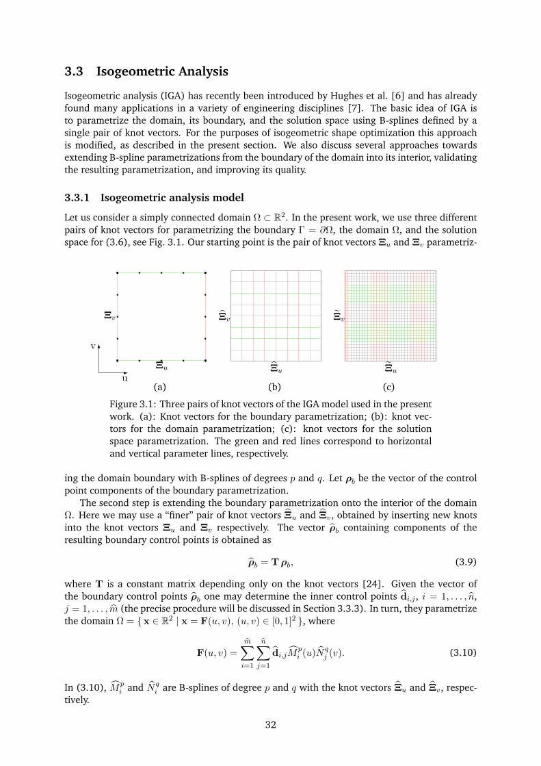
Isogeometric analysis (IGA) has recently been introduced by Hughes et al. [6] and has alreadyfound many applications in a variety of engineering disciplines [7]. The basic idea of IGA isto parametrize the domain, its boundary, and the solution space using B-splines defined by asingle pair of knot vectors. For the purposes of isogeometric shape optimization this approachis modified, as described in the present section. We also discuss several approaches towardsextending B-spline parametrizations from the boundary of the domain into its interior, validatingthe resulting parametrization, and improving its quality.
3.3.1 Isogeometric analysis model
Let us consider a simply connected domain Ω ⊂ R2. In the present work, we use three differentpairs of knot vectors for parametrizing the boundary Γ = ∂Ω, the domain Ω, and the solutionspace for (3.6), see Fig. 3.1. Our starting point is the pair of knot vectors Ξu and Ξv parametriz-
Ξu
Ξv
Ξu
Ξv
Ξu
Ξv
-
6
u
v
(a) (b) (c)
Figure 3.1: Three pairs of knot vectors of the IGA model used in the presentwork. (a): Knot vectors for the boundary parametrization; (b): knot vec-tors for the domain parametrization; (c): knot vectors for the solutionspace parametrization. The green and red lines correspond to horizontaland vertical parameter lines, respectively.
ing the domain boundary with B-splines of degrees p and q. Let ρb be the vector of the controlpoint components of the boundary parametrization.
The second step is extending the boundary parametrization onto the interior of the domainΩ. Here we may use a “finer” pair of knot vectors Ξu and Ξv, obtained by inserting new knotsinto the knot vectors Ξu and Ξv respectively. The vector ρb containing components of theresulting boundary control points is obtained as
ρb = Tρb, (3.9)
where T is a constant matrix depending only on the knot vectors [24]. Given the vector ofthe boundary control points ρb one may determine the inner control points di,j , i = 1, . . . , n,j = 1, . . . , m (the precise procedure will be discussed in Section 3.3.3). In turn, they parametrizethe domain Ω = x ∈ R2 | x = F(u, v), (u, v) ∈ [0, 1]2 , where
F(u, v) =
m∑
i=1
n∑
j=1
di,jMpi (u)N q
j (v). (3.10)
In (3.10), Mpi and N q
i are B-splines of degree p and q with the knot vectors Ξu and Ξv, respec-tively.
32
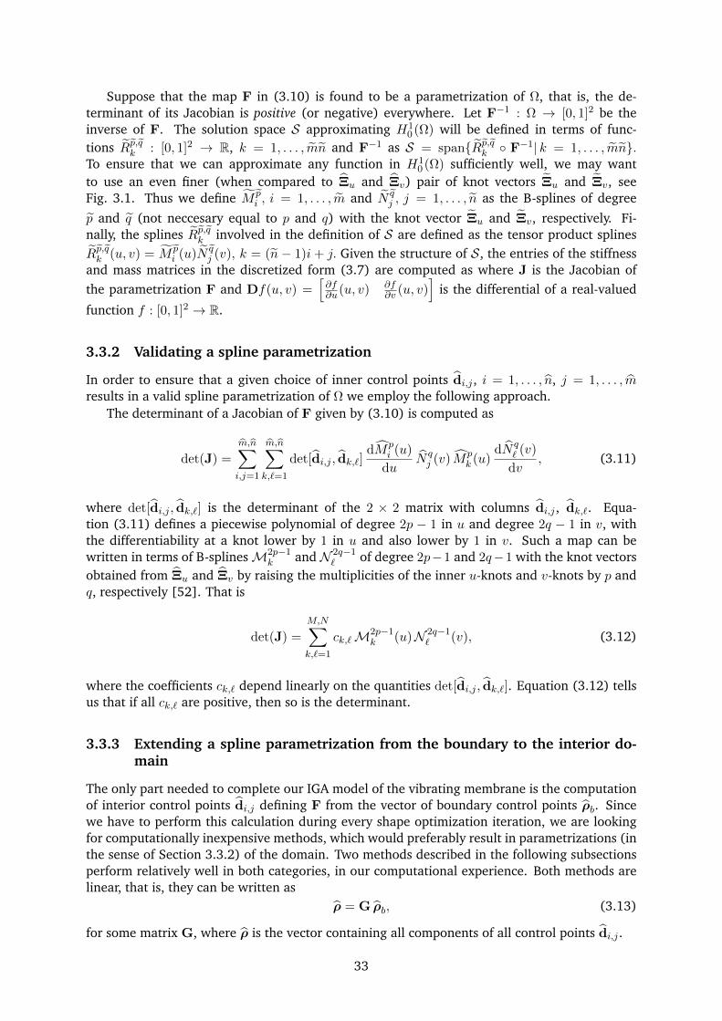
Suppose that the map F in (3.10) is found to be a parametrization of Ω, that is, the de-terminant of its Jacobian is positive (or negative) everywhere. Let F−1 : Ω → [0, 1]2 be theinverse of F. The solution space S approximating H1
0 (Ω) will be defined in terms of func-tions Rp,qk : [0, 1]2 → R, k = 1, . . . , mn and F−1 as S = spanRp,qk F−1| k = 1, . . . , mn.To ensure that we can approximate any function in H1
0 (Ω) sufficiently well, we may wantto use an even finer (when compared to Ξu and Ξv) pair of knot vectors Ξu and Ξv, seeFig. 3.1. Thus we define M p
i , i = 1, . . . , m and N qj , j = 1, . . . , n as the B-splines of degree
p and q (not neccesary equal to p and q) with the knot vector Ξu and Ξv, respectively. Fi-nally, the splines Rp,qk involved in the definition of S are defined as the tensor product splinesRp,qk (u, v) = M p
i (u)N qj (v), k = (n− 1)i+ j. Given the structure of S, the entries of the stiffness
and mass matrices in the discretized form (3.7) are computed as where J is the Jacobian ofthe parametrization F and Df(u, v) =
[∂f∂u(u, v) ∂f
∂v (u, v)]
is the differential of a real-valued
function f : [0, 1]2 → R.
3.3.2 Validating a spline parametrization
In order to ensure that a given choice of inner control points di,j , i = 1, . . . , n, j = 1, . . . , mresults in a valid spline parametrization of Ω we employ the following approach.
The determinant of a Jacobian of F given by (3.10) is computed as
det(J) =
m,n∑
i,j=1
m,n∑
k,`=1
det[di,j , dk,`]dMp
i (u)
duN qj (v) Mp
k (u)dN q
` (v)
dv, (3.11)
where det[di,j , dk,`] is the determinant of the 2 × 2 matrix with columns di,j , dk,`. Equa-tion (3.11) defines a piecewise polynomial of degree 2p − 1 in u and degree 2q − 1 in v, withthe differentiability at a knot lower by 1 in u and also lower by 1 in v. Such a map can bewritten in terms of B-splinesM2p−1
k and N 2q−1` of degree 2p−1 and 2q−1 with the knot vectors
obtained from Ξu and Ξv by raising the multiplicities of the inner u-knots and v-knots by p andq, respectively [52]. That is
det(J) =
M,N∑
k,`=1
ck,`M2p−1k (u)N 2q−1
` (v), (3.12)
where the coefficients ck,` depend linearly on the quantities det[di,j , dk,`]. Equation (3.12) tellsus that if all ck,` are positive, then so is the determinant.
3.3.3 Extending a spline parametrization from the boundary to the interior do-main
The only part needed to complete our IGA model of the vibrating membrane is the computationof interior control points di,j defining F from the vector of boundary control points ρb. Sincewe have to perform this calculation during every shape optimization iteration, we are lookingfor computationally inexpensive methods, which would preferably result in parametrizations (inthe sense of Section 3.3.2) of the domain. Two methods described in the following subsectionsperform relatively well in both categories, in our computational experience. Both methods arelinear, that is, they can be written as
ρ = G ρb, (3.13)
for some matrix G, where ρ is the vector containing all components of all control points di,j .
33
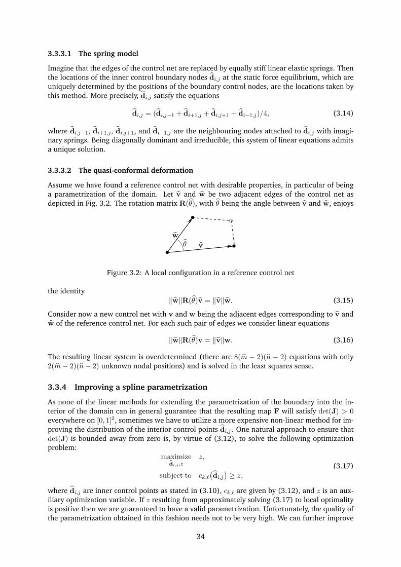
3.3.3.1 The spring model
Imagine that the edges of the control net are replaced by equally stiff linear elastic springs. Thenthe locations of the inner control boundary nodes di,j at the static force equilibrium, which areuniquely determined by the positions of the boundary control nodes, are the locations taken bythis method. More precisely, di,j satisfy the equations
di,j = (di,j−1 + di+1,j + di,j+1 + di−1,j)/4, (3.14)
where di,j−1, di+1,j , di,j+1, and di−1,j are the neighbouring nodes attached to di,j with imagi-nary springs. Being diagonally dominant and irreducible, this system of linear equations admitsa unique solution.
3.3.3.2 The quasi-conformal deformation
Assume we have found a reference control net with desirable properties, in particular of beinga parametrization of the domain. Let v and w be two adjacent edges of the control net asdepicted in Fig. 3.2. The rotation matrix R(θ), with θ being the angle between v and w, enjoys
v
wθ
Figure 3.2: A local configuration in a reference control net
the identity‖w‖R(θ)v = ‖v‖w. (3.15)
Consider now a new control net with v and w being the adjacent edges corresponding to v andw of the reference control net. For each such pair of edges we consider linear equations
‖w‖R(θ)v = ‖v‖w. (3.16)
The resulting linear system is overdetermined (there are 8(m − 2)(n − 2) equations with only2(m− 2)(n− 2) unknown nodal positions) and is solved in the least squares sense.
3.3.4 Improving a spline parametrization
As none of the linear methods for extending the parametrization of the boundary into the in-terior of the domain can in general guarantee that the resulting map F will satisfy det(J) > 0everywhere on [0, 1]2, sometimes we have to utilize a more expensive non-linear method for im-proving the distribution of the interior control points di,j . One natural approach to ensure thatdet(J) is bounded away from zero is, by virtue of (3.12), to solve the following optimizationproblem:
maximizedi,j ,z
z,
subject to ck,`(di,j)≥ z,
(3.17)
where di,j are inner control points as stated in (3.10), ck,` are given by (3.12), and z is an aux-iliary optimization variable. If z resulting from approximately solving (3.17) to local optimalityis positive then we are guaranteed to have a valid parametrization. Unfortunately, the quality ofthe parametrization obtained in this fashion needs not to be very high. We can further improve
34
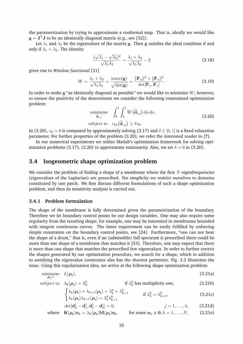
the parametrization by trying to approximate a conformal map. That is, ideally we would likeg = JTJ to be an identically diagonal matrix (e.g., see [32]).
Let λ1 and λ2 be the eigenvalues of the matrix g. Then g satisfies the ideal condition if andonly if λ1 = λ2. The identity
(√λ1 −
√λ2)2
√λ1λ2
=λ1 + λ2√λ1λ2
− 2 (3.18)
gives rise to Winslow functional [31]
W =λ1 + λ2√λ1λ2
=trace(g)√
det(g)=‖Fu‖2 + ‖Fv‖2
det[Fu,Fv]. (3.19)
In order to make g “as identically diagonal as possible” we would like to minimize W ; however,to ensure the positivity of the determinant we consider the following constrained optimizationproblem:
minimizedi,j
∫ 1
0
∫ 1
0W(di,j)
dudv,
subject to ck`(di,j)≥ δz0.
(3.20)
In (3.20), z0 > 0 is computed by approximately solving (3.17) and δ ∈ [0, 1] is a fixed relaxationparameter. For further properties of the problem (3.20), we refer the interested reader to [?].
In our numerical experiments we utilize Matlab’s optimization framework for solving opti-mization problems (3.17), (3.20) to approximate stationarity. Also, we set δ = 0 in (3.20).
3.4 Isogeometric shape optimization problem
We consider the problem of finding a shape of a membrane where the first N eigenfrequencies(eigenvalues of the Laplacian) are prescribed. For simplicity we restrict ourselves to domainsconstituted by one patch. We first discuss different formulations of such a shape optimizationproblem, and then its sensitivity analysis is carried out.
3.4.1 Problem formulation
The shape of the membrane is fully determined given the parametrization of the boundary.Therefore we let boundary control points be our design variables. One may also require someregularity from the resulting shape; for example, one may be interested in membranes boundedwith tangent continuous curves. The latter requirement can be easily fulfilled by enforcingsimple constraints on the boundary control points, see [24]. Furthermore, “one can not hearthe shape of a drum,” that is, even if an (admissible) full spectrum is prescribed there could bemore than one shape of a membrane that matches it [53]. Therefore, one may expect that thereis more than one shape that matches the prescribed few eigenvalues. In order to further restrictthe shapes generated by our optimization procedure, we search for a shape, which in additionto satisfying the eigenvalue constraints also has the shortest perimeter. Fig. 3.3 illustrates theissue. Using this regularization idea, we arrive at the following shape optimization problem:
minimizeρb,z
L(ρb), (3.21a)
subject to λk(ρb) = λ0k, if λ0
k has multiplicity one, (3.21b)λk(ρb) + λk+1(ρb) = λ0
k + λ0k+1
λk(ρb)λk+1(ρb) = λ0kλ
0k+1
if λ0k = λ0
k+1, (3.21c)
det[dj2 − dj1,dj2 − dj3] = 0, j = 1, . . . , 4, (3.21d)
where K(ρb)uk = λk(ρb)M(ρb)uk, for some uk 6= 0, k = 1, . . . , N, (3.21e)
35
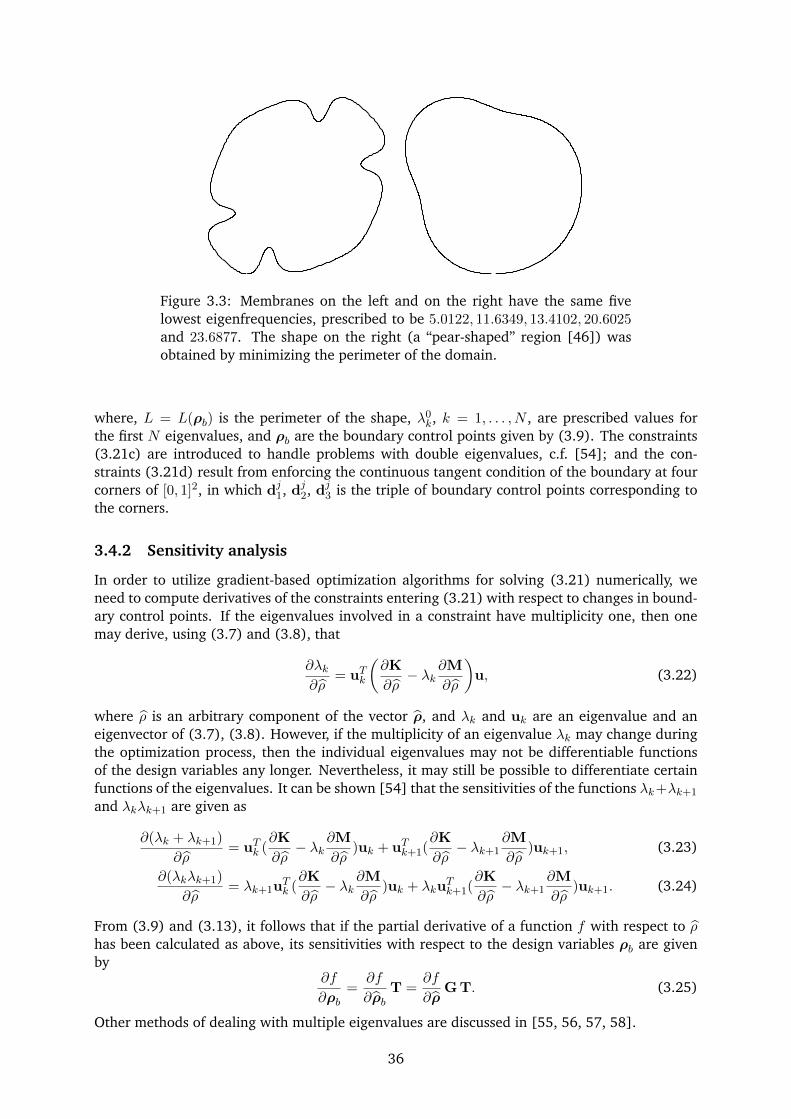
Figure 3.3: Membranes on the left and on the right have the same fivelowest eigenfrequencies, prescribed to be 5.0122, 11.6349, 13.4102, 20.6025and 23.6877. The shape on the right (a “pear-shaped” region [46]) wasobtained by minimizing the perimeter of the domain.
where, L = L(ρb) is the perimeter of the shape, λ0k, k = 1, . . . , N , are prescribed values for
the first N eigenvalues, and ρb are the boundary control points given by (3.9). The constraints(3.21c) are introduced to handle problems with double eigenvalues, c.f. [54]; and the con-straints (3.21d) result from enforcing the continuous tangent condition of the boundary at fourcorners of [0, 1]2, in which dj1, dj2, dj3 is the triple of boundary control points corresponding tothe corners.
3.4.2 Sensitivity analysis
In order to utilize gradient-based optimization algorithms for solving (3.21) numerically, weneed to compute derivatives of the constraints entering (3.21) with respect to changes in bound-ary control points. If the eigenvalues involved in a constraint have multiplicity one, then onemay derive, using (3.7) and (3.8), that
∂λk∂ρ
= uTk
(∂K
∂ρ− λk
∂M
∂ρ
)u, (3.22)
where ρ is an arbitrary component of the vector ρ, and λk and uk are an eigenvalue and aneigenvector of (3.7), (3.8). However, if the multiplicity of an eigenvalue λk may change duringthe optimization process, then the individual eigenvalues may not be differentiable functionsof the design variables any longer. Nevertheless, it may still be possible to differentiate certainfunctions of the eigenvalues. It can be shown [54] that the sensitivities of the functions λk+λk+1
and λkλk+1 are given as
∂(λk + λk+1)
∂ρ= uTk (
∂K
∂ρ− λk
∂M
∂ρ)uk + uTk+1(
∂K
∂ρ− λk+1
∂M
∂ρ)uk+1, (3.23)
∂(λkλk+1)
∂ρ= λk+1u
Tk (∂K
∂ρ− λk
∂M
∂ρ)uk + λku
Tk+1(
∂K
∂ρ− λk+1
∂M
∂ρ)uk+1. (3.24)
From (3.9) and (3.13), it follows that if the partial derivative of a function f with respect to ρhas been calculated as above, its sensitivities with respect to the design variables ρb are givenby
∂f
∂ρb=
∂f
∂ρbT =
∂f
∂ρG T. (3.25)
Other methods of dealing with multiple eigenvalues are discussed in [55, 56, 57, 58].
36
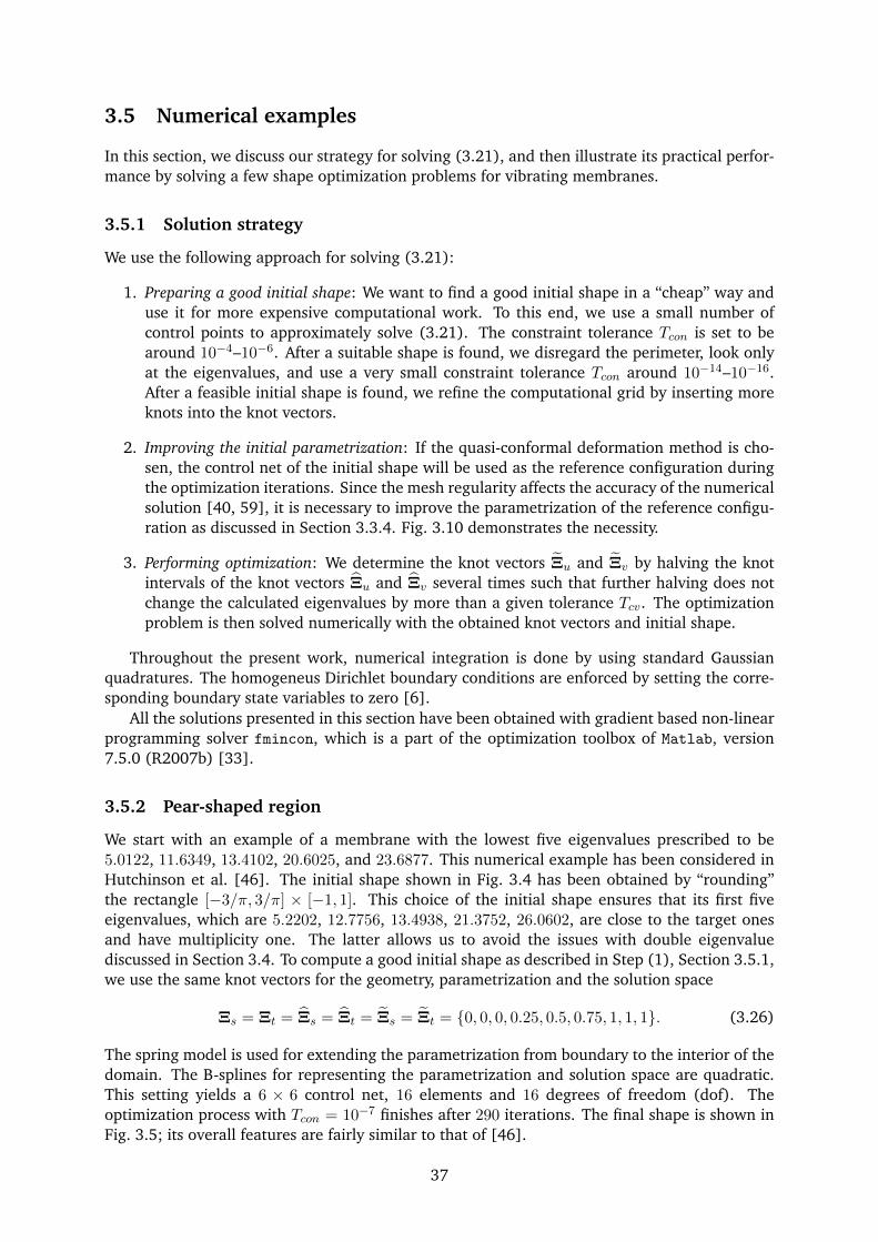
3.5 Numerical examples
In this section, we discuss our strategy for solving (3.21), and then illustrate its practical perfor-mance by solving a few shape optimization problems for vibrating membranes.
3.5.1 Solution strategy
We use the following approach for solving (3.21):
1. Preparing a good initial shape: We want to find a good initial shape in a “cheap” way anduse it for more expensive computational work. To this end, we use a small number ofcontrol points to approximately solve (3.21). The constraint tolerance Tcon is set to bearound 10−4–10−6. After a suitable shape is found, we disregard the perimeter, look onlyat the eigenvalues, and use a very small constraint tolerance Tcon around 10−14–10−16.After a feasible initial shape is found, we refine the computational grid by inserting moreknots into the knot vectors.
2. Improving the initial parametrization: If the quasi-conformal deformation method is cho-sen, the control net of the initial shape will be used as the reference configuration duringthe optimization iterations. Since the mesh regularity affects the accuracy of the numericalsolution [40, 59], it is necessary to improve the parametrization of the reference configu-ration as discussed in Section 3.3.4. Fig. 3.10 demonstrates the necessity.
3. Performing optimization: We determine the knot vectors Ξu and Ξv by halving the knotintervals of the knot vectors Ξu and Ξv several times such that further halving does notchange the calculated eigenvalues by more than a given tolerance Tcv. The optimizationproblem is then solved numerically with the obtained knot vectors and initial shape.
Throughout the present work, numerical integration is done by using standard Gaussianquadratures. The homogeneus Dirichlet boundary conditions are enforced by setting the corre-sponding boundary state variables to zero [6].
All the solutions presented in this section have been obtained with gradient based non-linearprogramming solver fmincon, which is a part of the optimization toolbox of Matlab, version7.5.0 (R2007b) [33].
3.5.2 Pear-shaped region
We start with an example of a membrane with the lowest five eigenvalues prescribed to be5.0122, 11.6349, 13.4102, 20.6025, and 23.6877. This numerical example has been considered inHutchinson et al. [46]. The initial shape shown in Fig. 3.4 has been obtained by “rounding”the rectangle [−3/π, 3/π] × [−1, 1]. This choice of the initial shape ensures that its first fiveeigenvalues, which are 5.2202, 12.7756, 13.4938, 21.3752, 26.0602, are close to the target onesand have multiplicity one. The latter allows us to avoid the issues with double eigenvaluediscussed in Section 3.4. To compute a good initial shape as described in Step (1), Section 3.5.1,we use the same knot vectors for the geometry, parametrization and the solution space
Ξs = Ξt = Ξs = Ξt = Ξs = Ξt = 0, 0, 0, 0.25, 0.5, 0.75, 1, 1, 1. (3.26)
The spring model is used for extending the parametrization from boundary to the interior of thedomain. The B-splines for representing the parametrization and solution space are quadratic.This setting yields a 6 × 6 control net, 16 elements and 16 degrees of freedom (dof). Theoptimization process with Tcon = 10−7 finishes after 290 iterations. The final shape is shown inFig. 3.5; its overall features are fairly similar to that of [46].
37
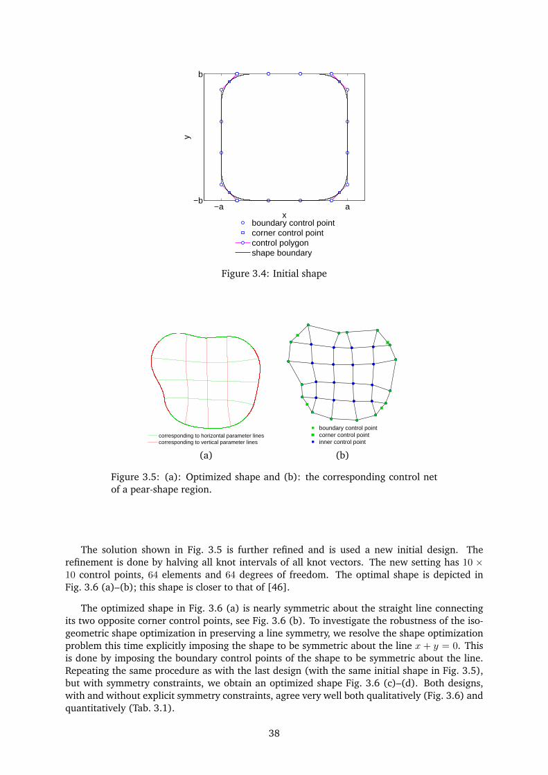
−a a−b
b
x
y
boundary control pointcorner control pointcontrol polygonshape boundary
Figure 3.4: Initial shape
corresponding to horizontal parameter linescorresponding to vertical parameter lines
boundary control pointcorner control pointinner control point
(a) (b)
Figure 3.5: (a): Optimized shape and (b): the corresponding control netof a pear-shape region.
The solution shown in Fig. 3.5 is further refined and is used a new initial design. Therefinement is done by halving all knot intervals of all knot vectors. The new setting has 10 ×10 control points, 64 elements and 64 degrees of freedom. The optimal shape is depicted inFig. 3.6 (a)–(b); this shape is closer to that of [46].
The optimized shape in Fig. 3.6 (a) is nearly symmetric about the straight line connectingits two opposite corner control points, see Fig. 3.6 (b). To investigate the robustness of the iso-geometric shape optimization in preserving a line symmetry, we resolve the shape optimizationproblem this time explicitly imposing the shape to be symmetric about the line x + y = 0. Thisis done by imposing the boundary control points of the shape to be symmetric about the line.Repeating the same procedure as with the last design (with the same initial shape in Fig. 3.5),but with symmetry constraints, we obtain an optimized shape Fig. 3.6 (c)–(d). Both designs,with and without explicit symmetry constraints, agree very well both qualitatively (Fig. 3.6) andquantitatively (Tab. 3.1).
38
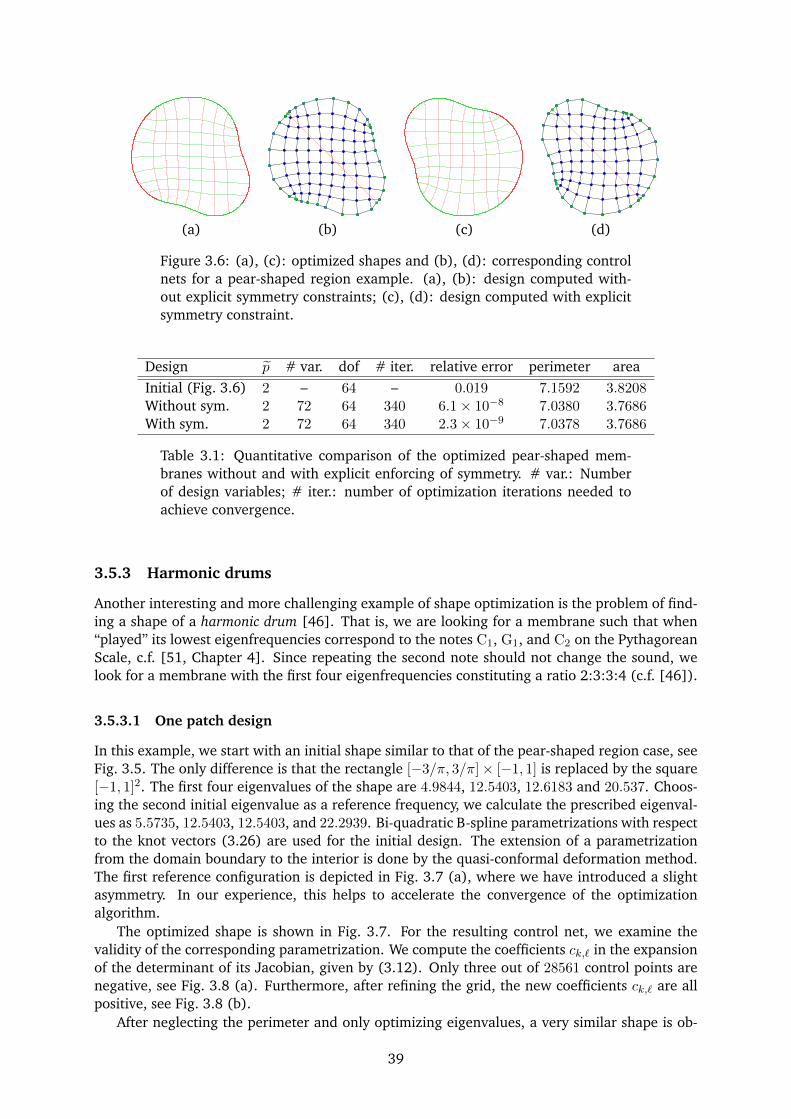
(a) (b) (c) (d)
Figure 3.6: (a), (c): optimized shapes and (b), (d): corresponding controlnets for a pear-shaped region example. (a), (b): design computed with-out explicit symmetry constraints; (c), (d): design computed with explicitsymmetry constraint.
Design p # var. dof # iter. relative error perimeter areaInitial (Fig. 3.6) 2 – 64 – 0.019 7.1592 3.8208Without sym. 2 72 64 340 6.1× 10⁻⁸ 7.0380 3.7686With sym. 2 72 64 340 2.3× 10⁻⁹ 7.0378 3.7686
Table 3.1: Quantitative comparison of the optimized pear-shaped mem-branes without and with explicit enforcing of symmetry. # var.: Numberof design variables; # iter.: number of optimization iterations needed toachieve convergence.
3.5.3 Harmonic drums
Another interesting and more challenging example of shape optimization is the problem of find-ing a shape of a harmonic drum [46]. That is, we are looking for a membrane such that when“played” its lowest eigenfrequencies correspond to the notes C1, G1, and C2 on the PythagoreanScale, c.f. [51, Chapter 4]. Since repeating the second note should not change the sound, welook for a membrane with the first four eigenfrequencies constituting a ratio 2:3:3:4 (c.f. [46]).
3.5.3.1 One patch design
In this example, we start with an initial shape similar to that of the pear-shaped region case, seeFig. 3.5. The only difference is that the rectangle [−3/π, 3/π]× [−1, 1] is replaced by the square[−1, 1]2. The first four eigenvalues of the shape are 4.9844, 12.5403, 12.6183 and 20.537. Choos-ing the second initial eigenvalue as a reference frequency, we calculate the prescribed eigenval-ues as 5.5735, 12.5403, 12.5403, and 22.2939. Bi-quadratic B-spline parametrizations with respectto the knot vectors (3.26) are used for the initial design. The extension of a parametrizationfrom the domain boundary to the interior is done by the quasi-conformal deformation method.The first reference configuration is depicted in Fig. 3.7 (a), where we have introduced a slightasymmetry. In our experience, this helps to accelerate the convergence of the optimizationalgorithm.
The optimized shape is shown in Fig. 3.7. For the resulting control net, we examine thevalidity of the corresponding parametrization. We compute the coefficients ck,` in the expansionof the determinant of its Jacobian, given by (3.12). Only three out of 28561 control points arenegative, see Fig. 3.8 (a). Furthermore, after refining the grid, the new coefficients ck,` are allpositive, see Fig. 3.8 (b).
After neglecting the perimeter and only optimizing eigenvalues, a very similar shape is ob-
39
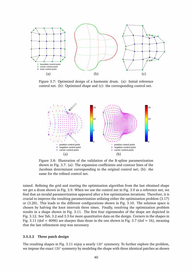
boundary control pointcorner control pointinner control point
(a) (b) (c)
Figure 3.7: Optimized design of a harmonic drum. (a): Initial referencecontrol net. (b): Optimized shape and (c): the corresponding control net.
positive control pointnegative control pointcorner control point
0
5
10
15
positive control pointnegative control pointcorner control point
0
5
10
15
@@@I
(a) (b)
Figure 3.8: Illustration of the validation of the B-spline parametrizationshown in Fig. 3.7. (a): The expansion coefficients and contour lines of theJacobian determinant corresponding to the original control net; (b): thesame for the refined control net.
tained. Refining the grid and starting the optimization algorithm from the last obtained shapewe get a drum shown in Fig. 3.9. When we use the control net in Fig. 3.9 as a reference net, wefind that an invalid parametrization appeared after a few optimization iterations. Therefore, it iscrucial to improve the resulting parametrization utilizing either the optimization problem (3.17)or (3.20). This leads to the different configurations shown in Fig. 3.10. The solution space ischosen by halving the knot intervals three times. Finally, resolving the optimization problemresults in a shape shown in Fig. 3.11. The first four eigenmodes of the shape are depicted inFig. 3.12. See Tab. 3.2 and 3.3 for more quantitative data on the design. Corners in the shapes inFig. 3.11 (dof = 4096) are sharper than those in the one shown in Fig. 3.7 (dof = 16), meaningthat the last refinement step was necessary.
3.5.3.2 Three patch design
The resulting shapes in Fig. 3.11 enjoy a nearly 120 symmetry. To further explore the problem,we impose the exact 120 symmetry by modeling the shape with three identical patches as shown
40
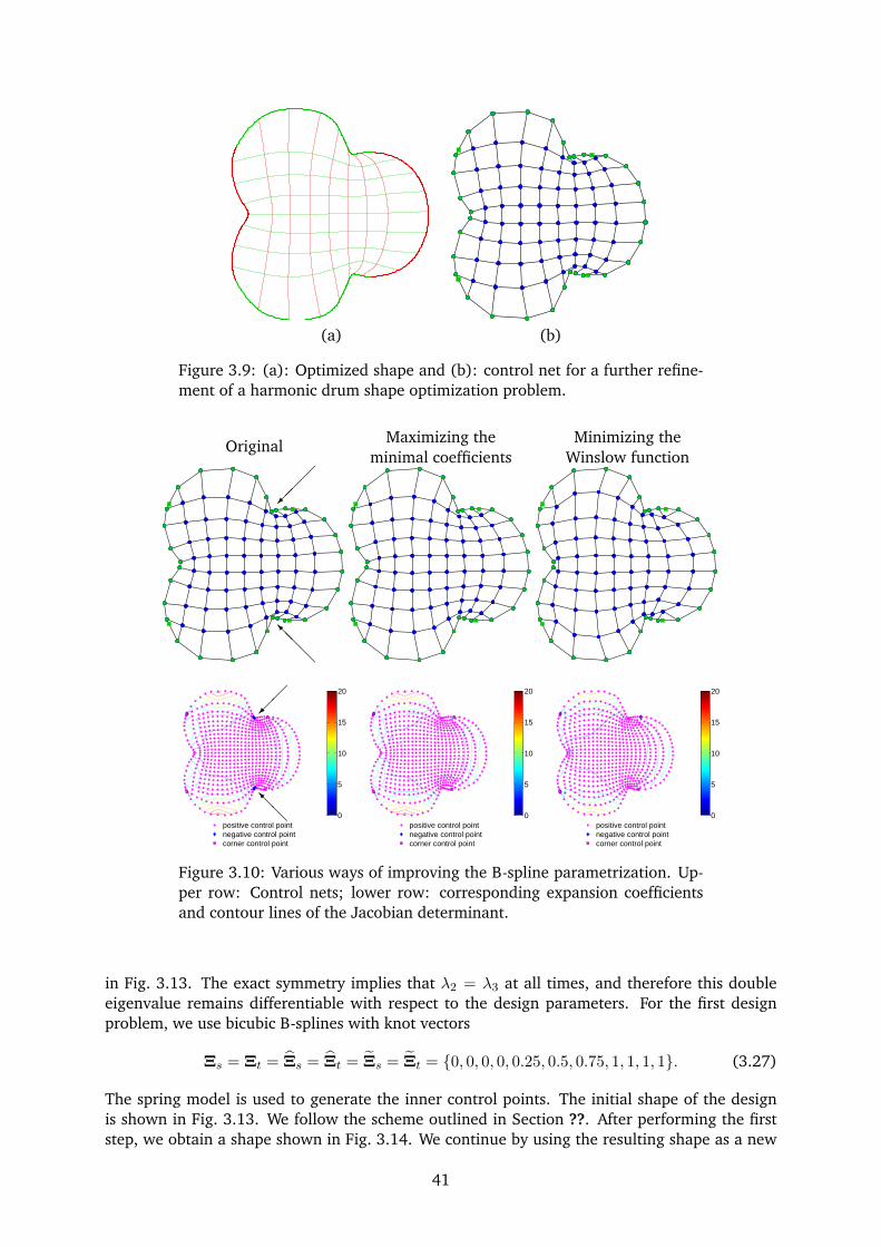
(a) (b)
Figure 3.9: (a): Optimized shape and (b): control net for a further refine-ment of a harmonic drum shape optimization problem.
Original Maximizing theminimal coefficients
Minimizing theWinslow function
positive control pointnegative control pointcorner control point
0
5
10
15
20
positive control pointnegative control pointcorner control point
0
5
10
15
20
positive control pointnegative control pointcorner control point
0
5
10
15
20
@@I
@@@I
Figure 3.10: Various ways of improving the B-spline parametrization. Up-per row: Control nets; lower row: corresponding expansion coefficientsand contour lines of the Jacobian determinant.
in Fig. 3.13. The exact symmetry implies that λ2 = λ3 at all times, and therefore this doubleeigenvalue remains differentiable with respect to the design parameters. For the first designproblem, we use bicubic B-splines with knot vectors
Ξs = Ξt = Ξs = Ξt = Ξs = Ξt = 0, 0, 0, 0, 0.25, 0.5, 0.75, 1, 1, 1, 1. (3.27)
The spring model is used to generate the inner control points. The initial shape of the designis shown in Fig. 3.13. We follow the scheme outlined in Section ??. After performing the firststep, we obtain a shape shown in Fig. 3.14. We continue by using the resulting shape as a new
41
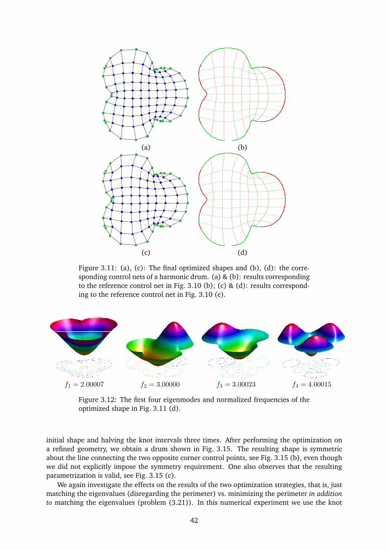
(a) (b)
(c) (d)
Figure 3.11: (a), (c): The final optimized shapes and (b), (d): the corre-sponding control nets of a harmonic drum. (a) & (b): results correspondingto the reference control net in Fig. 3.10 (b); (c) & (d): results correspond-ing to the reference control net in Fig. 3.10 (c).
f1 = 2.00007 f2 = 3.00000 f3 = 3.00023 f4 = 4.00015
Figure 3.12: The first four eigenmodes and normalized frequencies of theoptimized shape in Fig. 3.11 (d).
initial shape and halving the knot intervals three times. After performing the optimization ona refined geometry, we obtain a drum shown in Fig. 3.15. The resulting shape is symmetricabout the line connecting the two opposite corner control points, see Fig. 3.15 (b), even thoughwe did not explicitly impose the symmetry requirement. One also observes that the resultingparametrization is valid, see Fig. 3.15 (c).
We again investigate the effects on the results of the two optimization strategies, that is, justmatching the eigenvalues (disregarding the perimeter) vs. minimizing the perimeter in additionto matching the eigenvalues (problem (3.21)). In this numerical experiment we use the knot
42
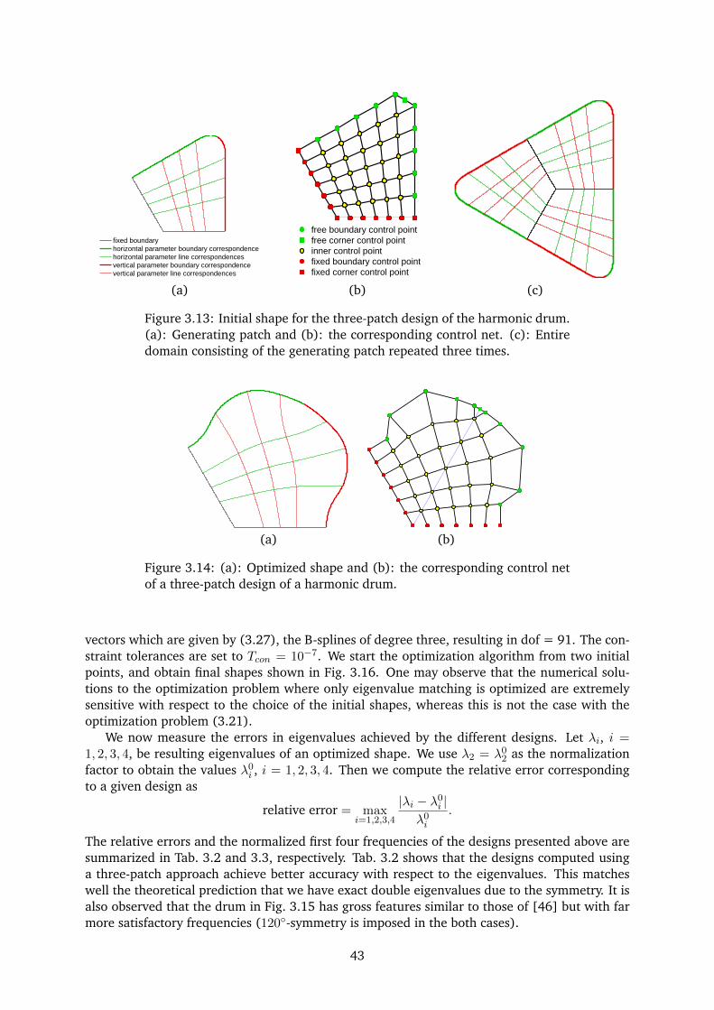
fixed boundaryhorizontal parameter boundary correspondencehorizontal parameter line correspondencesvertical parameter boundary correspondencevertical parameter line correspondences
free boundary control pointfree corner control pointinner control pointfixed boundary control pointfixed corner control point
(a) (b) (c)
Figure 3.13: Initial shape for the three-patch design of the harmonic drum.(a): Generating patch and (b): the corresponding control net. (c): Entiredomain consisting of the generating patch repeated three times.
(a) (b)
Figure 3.14: (a): Optimized shape and (b): the corresponding control netof a three-patch design of a harmonic drum.
vectors which are given by (3.27), the B-splines of degree three, resulting in dof = 91. The con-straint tolerances are set to Tcon = 10−7. We start the optimization algorithm from two initialpoints, and obtain final shapes shown in Fig. 3.16. One may observe that the numerical solu-tions to the optimization problem where only eigenvalue matching is optimized are extremelysensitive with respect to the choice of the initial shapes, whereas this is not the case with theoptimization problem (3.21).
We now measure the errors in eigenvalues achieved by the different designs. Let λi, i =1, 2, 3, 4, be resulting eigenvalues of an optimized shape. We use λ2 = λ0
2 as the normalizationfactor to obtain the values λ0
i , i = 1, 2, 3, 4. Then we compute the relative error correspondingto a given design as
relative error = maxi=1,2,3,4
|λi − λ0i |
λ0i
.
The relative errors and the normalized first four frequencies of the designs presented above aresummarized in Tab. 3.2 and 3.3, respectively. Tab. 3.2 shows that the designs computed usinga three-patch approach achieve better accuracy with respect to the eigenvalues. This matcheswell the theoretical prediction that we have exact double eigenvalues due to the symmetry. It isalso observed that the drum in Fig. 3.15 has gross features similar to those of [46] but with farmore satisfactory frequencies (120-symmetry is imposed in the both cases).
43
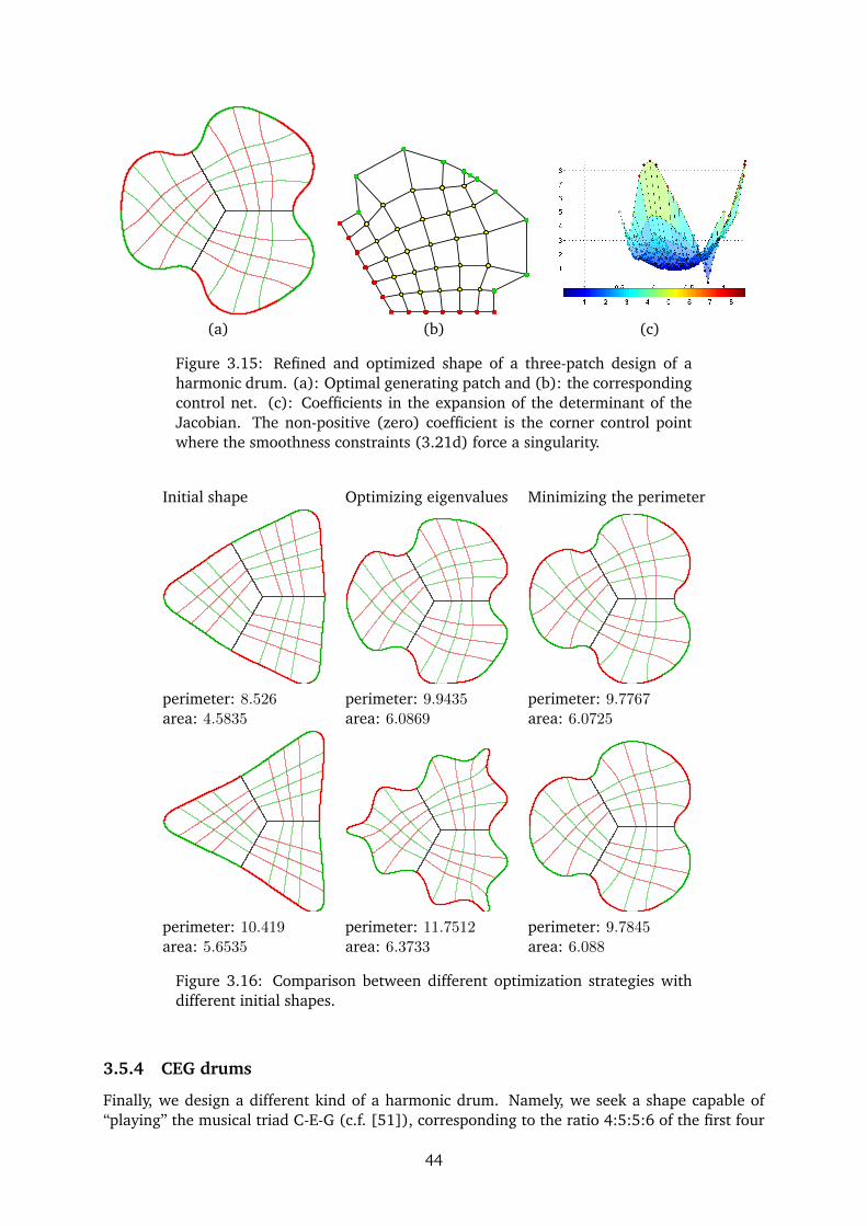
(a) (b) (c)
Figure 3.15: Refined and optimized shape of a three-patch design of aharmonic drum. (a): Optimal generating patch and (b): the correspondingcontrol net. (c): Coefficients in the expansion of the determinant of theJacobian. The non-positive (zero) coefficient is the corner control pointwhere the smoothness constraints (3.21d) force a singularity.
Initial shape Optimizing eigenvalues Minimizing the perimeter
perimeter: 8.526 perimeter: 9.9435 perimeter: 9.7767area: 4.5835 area: 6.0869 area: 6.0725
perimeter: 10.419 perimeter: 11.7512 perimeter: 9.7845area: 5.6535 area: 6.3733 area: 6.088
Figure 3.16: Comparison between different optimization strategies withdifferent initial shapes.
3.5.4 CEG drums
Finally, we design a different kind of a harmonic drum. Namely, we seek a shape capable of“playing” the musical triad C-E-G (c.f. [51]), corresponding to the ratio 4:5:5:6 of the first four
44
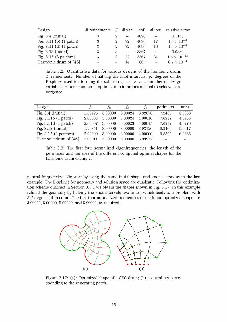
Design # refinements p # var. dof # iter. relative errorFig. 3.4 (initial) 3 2 – 4096 – 0.1148Fig. 3.11 (b) (1 patch) 3 2 72 4096 17 1.6× 10⁻⁴
Fig. 3.11 (d) (1 patch) 3 2 72 4096 16 1.6× 10⁻⁴
Fig. 3.13 (initial) 3 3 – 3367 – 0.0380Fig. 3.15 (3 patches) 3 3 22 3367 31 1.5× 10⁻¹³
Harmonic drum of [46] – – 14 60 – 0.7× 10⁻⁴
Table 3.2: Quantitative data for various designs of the harmonic drum.# refinements: Number of halving the knot intervals; p: degrees of theB-splines used for forming the solution space; # var.: number of designvariables; # iter.: number of optimization iterations needed to achieve con-vergence.
Design f1 f2 f3 f4 perimeter areaFig. 3.4 (initial) 1.89426 3.00000 3.00024 3.82078 7.2465 3.8333Fig. 3.11b (1 patch) 2.00008 3.00000 3.00024 4.00016 7.6232 4.0255Fig. 3.11d (1 patch) 2.00007 3.00000 3.00023 4.00015 7.6232 4.0276Fig. 3.13 (initial) 1.96351 3.00000 3.00000 3.93126 9.3460 5.0617Fig. 3.15 (3 patches) 2.00000 3.00000 3.00000 4.00000 9.8592 6.0686Harmonic drum of [46] 2.00011 3.00000 3.00000 3.99972 – –
Table 3.3: The first four normalized eigenfrequencies, the length of theperimeter, and the area of the different computed optimal shapes for theharmonic drum example.
natural frequencies. We start by using the same initial shape and knot vectors as in the lastexample. The B-splines for geometry and solution space are quadratic. Following the optimiza-tion scheme outlined in Section 3.5.1 we obtain the shapes shown in Fig. 3.17. In this examplerefined the geometry by halving the knot intervals two times, which leads to a problem with817 degrees of freedom. The first four normalized frequencies of the found optimized shape are3.99999, 5.00000, 5.00000, and 5.99999, as required.
(a) (b)
Figure 3.17: (a): Optimized shape of a CEG drum; (b): control net corre-sponding to the generating patch.
45
3.6 Conclusions
We have applied isogeometric analysis towards shape optimization problems of vibrating mem-branes, where we allow the shape of the domain to experience very large deformations. We haveused three different spline parametrizations for the boundary and the interior of the domains,as well as for the approximate solution space for the governing boundary value problem. Thisallows us to independently vary the number of control points for the shape parametrization andthe approximation properties of the discretization of the governing equations.
We have carried out numerical studies of several techniques for extending the domain parametriza-tion from the boundary to the interior and improving the quality of the domain parametrization.As a result, we have presented solutions to several eigenvalue optimization problems for theLaplace equation. Due to the properties of B-splines, some nice shapes have been obtained witha relatively small number of design variables. The problems have been solved numerically in anumber of different ways (for example, without and with explicit constraints ensuring certainsymmetries) yet they yielded the same optimal solutions, thus supporting the robustness of ourapproach.
46
Chapter 4
On the sensitivities of multipleeigenvalues
J. Gravesen, A. Evgrafov, Nguyen D. M., On the sensitivities of multiple eigenvalues, Structuraland Multidisciplinary Optimization, vol. 44, pp. 583-587, 2011.
Abstract. We consider the generalized symmetric eigenvalue problem where matrices dependsmoothly on a parameter. It is well known that in general individual eigenvalues, when sorted inaccordance with the usual ordering on the real line, do not depend smoothly on the parameter.Nevertheless, symmetric polynomials of a number of eigenvalues, regardless of their multiplicity,which are known to be isolated from the rest depend smoothly on the parameter. We presentexplicit readily computable expressions for their first derivatives. Finally, we demonstrate theutility of our approach on a problem of finding a shape of a vibrating membrane with a smallestperimeter and with prescribed four lowest eigenvalues, only two of which are have algebraicmultiplicity one.
Keywords: Multiple eigenvalues; sensitivity analysis.
4.1 Introduction
Consider a function A : R → S2 mapping a parameter t into a set of 2 × 2 symmetric matrices.Even when entries aij(t), i, j = 1, 2 depend smoothly on the parameter, the eigenvalues λ1(t) ≤λ2(t) may be non-smooth functions at points where their multiplicity changes. Nevertheless,both their sum λ1(t) + λ2(t) = trace A(t) = a11(t) + a22(t) and their product λ1(t)λ2(t) =det A(t) = a11(t) a22(t)− a12(t) a21(t) clearly remain smooth functions. This knowledge may beused to, for example, replace potentially non-smooth pair of constraints λ1(t) = λ1, λ2(t) = λ2,with a pair of smooth ones: trace A(t) = λ1 + λ2, det A(t) = λ1 λ2, see [9].
For 2 × 2 matrices explicit expressions for [trace A(t)]′ and [det A(t)]′, where with primethroughout the paper we denote differentiation with respect to t, may be easily obtained interms of aij(t), i, j = 1, 2, and their derivatives. However, we seek an alternative representationof these quantities, which remain valid for higher-dimensional problems. To this end, let u1 :R → R2, u2 : R → R2 be the normalized eigenvectors corresponding to λ1(t), λ2(t). Weassume a computationally realistic situation, when the vectors u1(t) and u2(t) are not necessarilycontinuous for t ∈ R such that λ1(t) = λ2(t). (Indeed, in our simple two-dimensional example anarbitrary pair of non-zero vectors u1(t) and u2(t) constitutes a pair of eigenvectors for t ∈ R suchthat λ1(t) = λ2(t).) However, we do assume that these vectors are chosen to be orthonormal forall t ∈ R. Whenever the function λi(t), i = 1, 2, is differentiable at a point t0 ∈ R, its derivative
47
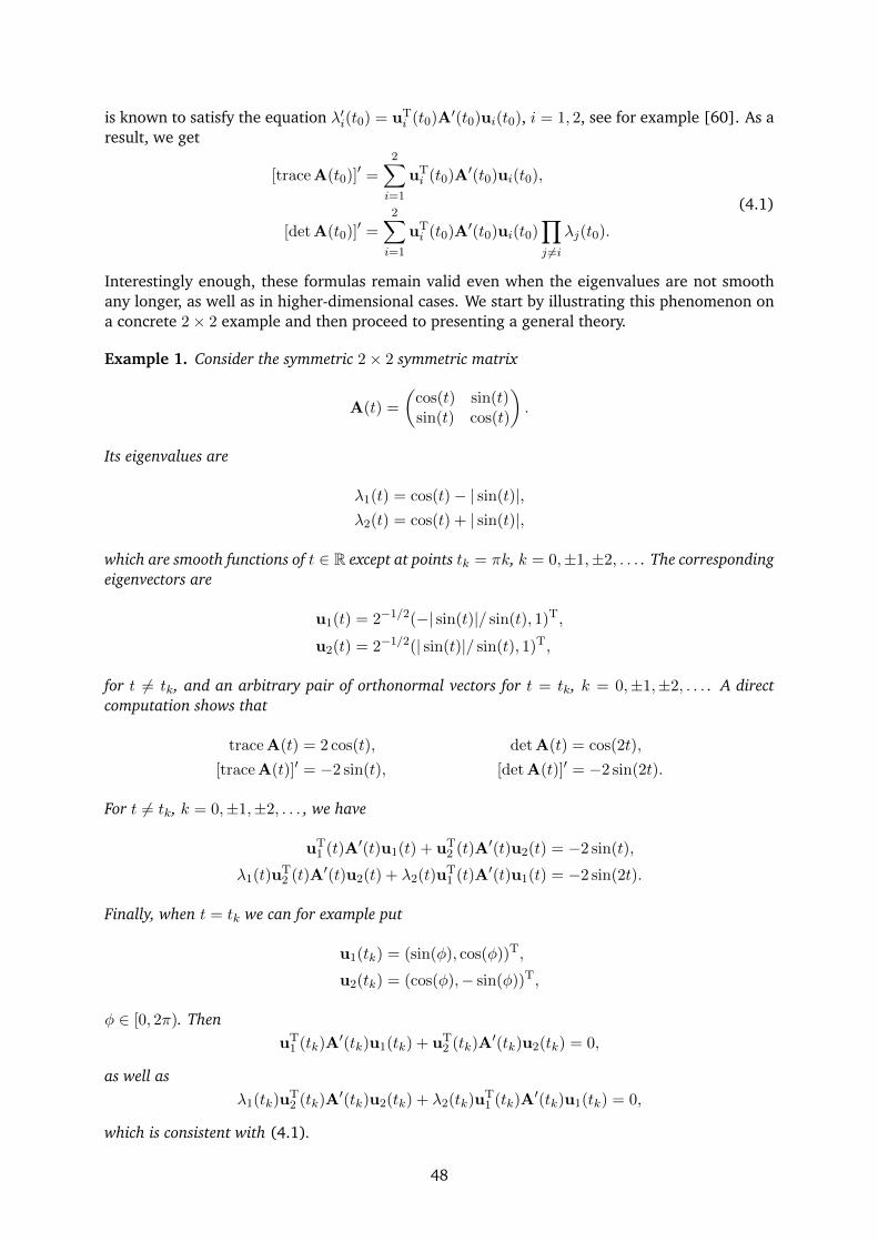
is known to satisfy the equation λ′i(t0) = uTi (t0)A′(t0)ui(t0), i = 1, 2, see for example [60]. As a
result, we get
[trace A(t0)]′ =2∑
i=1
uTi (t0)A′(t0)ui(t0),
[det A(t0)]′ =2∑
i=1
uTi (t0)A′(t0)ui(t0)
∏
j 6=iλj(t0).
(4.1)
Interestingly enough, these formulas remain valid even when the eigenvalues are not smoothany longer, as well as in higher-dimensional cases. We start by illustrating this phenomenon ona concrete 2× 2 example and then proceed to presenting a general theory.
Example 1. Consider the symmetric 2× 2 symmetric matrix
A(t) =
(cos(t) sin(t)sin(t) cos(t)
).
Its eigenvalues are
λ1(t) = cos(t)− | sin(t)|,λ2(t) = cos(t) + | sin(t)|,
which are smooth functions of t ∈ R except at points tk = πk, k = 0,±1,±2, . . . . The correspondingeigenvectors are
u1(t) = 2−1/2(−| sin(t)|/ sin(t), 1)T,
u2(t) = 2−1/2(| sin(t)|/ sin(t), 1)T,
for t 6= tk, and an arbitrary pair of orthonormal vectors for t = tk, k = 0,±1,±2, . . . . A directcomputation shows that
trace A(t) = 2 cos(t), det A(t) = cos(2t),
[trace A(t)]′ = −2 sin(t), [det A(t)]′ = −2 sin(2t).
For t 6= tk, k = 0,±1,±2, . . . , we have
uT1 (t)A′(t)u1(t) + uT
2 (t)A′(t)u2(t) = −2 sin(t),
λ1(t)uT2 (t)A′(t)u2(t) + λ2(t)uT
1 (t)A′(t)u1(t) = −2 sin(2t).
Finally, when t = tk we can for example put
u1(tk) = (sin(φ), cos(φ))T,
u2(tk) = (cos(φ),− sin(φ))T,
φ ∈ [0, 2π). ThenuT
1 (tk)A′(tk)u1(tk) + uT
2 (tk)A′(tk)u2(tk) = 0,
as well asλ1(tk)u
T2 (tk)A
′(tk)u2(tk) + λ2(tk)uT1 (tk)A
′(tk)u1(tk) = 0,
which is consistent with (4.1).
48
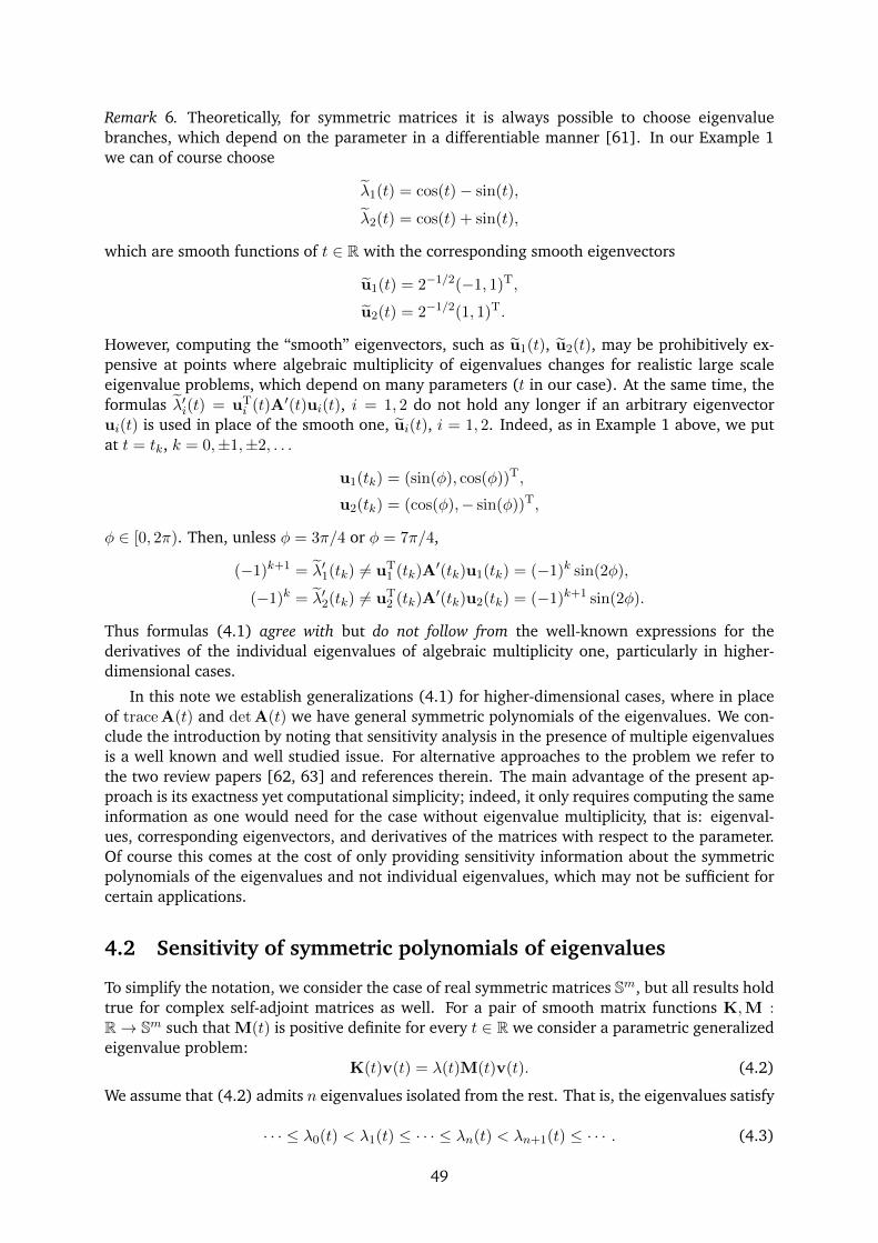
Remark 6. Theoretically, for symmetric matrices it is always possible to choose eigenvaluebranches, which depend on the parameter in a differentiable manner [61]. In our Example 1we can of course choose
λ1(t) = cos(t)− sin(t),
λ2(t) = cos(t) + sin(t),
which are smooth functions of t ∈ R with the corresponding smooth eigenvectors
u1(t) = 2−1/2(−1, 1)T,
u2(t) = 2−1/2(1, 1)T.
However, computing the “smooth” eigenvectors, such as u1(t), u2(t), may be prohibitively ex-pensive at points where algebraic multiplicity of eigenvalues changes for realistic large scaleeigenvalue problems, which depend on many parameters (t in our case). At the same time, theformulas λ′i(t) = uT
i (t)A′(t)ui(t), i = 1, 2 do not hold any longer if an arbitrary eigenvectorui(t) is used in place of the smooth one, ui(t), i = 1, 2. Indeed, as in Example 1 above, we putat t = tk, k = 0,±1,±2, . . .
u1(tk) = (sin(φ), cos(φ))T,
u2(tk) = (cos(φ),− sin(φ))T,
φ ∈ [0, 2π). Then, unless φ = 3π/4 or φ = 7π/4,
(−1)k+1 = λ′1(tk) 6= uT1 (tk)A
′(tk)u1(tk) = (−1)k sin(2φ),
(−1)k = λ′2(tk) 6= uT2 (tk)A
′(tk)u2(tk) = (−1)k+1 sin(2φ).
Thus formulas (4.1) agree with but do not follow from the well-known expressions for thederivatives of the individual eigenvalues of algebraic multiplicity one, particularly in higher-dimensional cases.
In this note we establish generalizations (4.1) for higher-dimensional cases, where in placeof trace A(t) and det A(t) we have general symmetric polynomials of the eigenvalues. We con-clude the introduction by noting that sensitivity analysis in the presence of multiple eigenvaluesis a well known and well studied issue. For alternative approaches to the problem we refer tothe two review papers [62, 63] and references therein. The main advantage of the present ap-proach is its exactness yet computational simplicity; indeed, it only requires computing the sameinformation as one would need for the case without eigenvalue multiplicity, that is: eigenval-ues, corresponding eigenvectors, and derivatives of the matrices with respect to the parameter.Of course this comes at the cost of only providing sensitivity information about the symmetricpolynomials of the eigenvalues and not individual eigenvalues, which may not be sufficient forcertain applications.
4.2 Sensitivity of symmetric polynomials of eigenvalues
To simplify the notation, we consider the case of real symmetric matrices Sm, but all results holdtrue for complex self-adjoint matrices as well. For a pair of smooth matrix functions K,M :R→ Sm such that M(t) is positive definite for every t ∈ R we consider a parametric generalizedeigenvalue problem:
K(t)v(t) = λ(t)M(t)v(t). (4.2)
We assume that (4.2) admits n eigenvalues isolated from the rest. That is, the eigenvalues satisfy
· · · ≤ λ0(t) < λ1(t) ≤ · · · ≤ λn(t) < λn+1(t) ≤ · · · . (4.3)
49
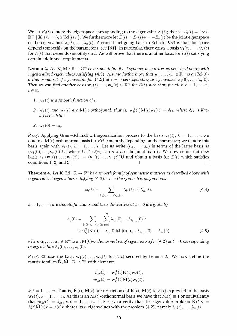
We let Ei(t) denote the eigenspace corresponding to the eigenvalue λi(t); that is, Ei(t) = v ∈Rm | K(t)v = λi(t)M(t)v . We furthermore letE(t) = E1(t)+· · ·+En(t) be the joint eigenspaceof the eigenvalues λ1(t), . . . , λn(t). A crucial fact going back to Rellich 1953 is that this spacedepends smoothly on the parameter t, see [61]. In particular, there exists a basis v1(t), . . . ,vn(t)for E(t) that depends smoothly on t. We will prove that there is another basis for E(t) satisfyingcertain additional requirements.
Lemma 2. Let K,M : R→ Sm be a smooth family of symmetric matrices as described above withn generalized eigenvalues satisfying (4.3). Assume furthermore that u1, . . . ,un ∈ Rm is an M(0)-orthonormal set of eigenvectors for (4.2) at t = 0 corresponding to eigenvalues λ1(0), . . . , λn(0).Then we can find another basis w1(t), . . . ,wn(t) ∈ Rm for E(t) such that, for all k, ` = 1, . . . , n,t ∈ R:
1. wk(t) is a smooth function of t;
2. wk(t) and w`(t) are M(t)-orthogonal, that is, wTk (t)M(t)w`(t) = δk`, where δk` is Kro-
necker’s delta;
3. wk(0) = uk.
Proof. Applying Gram–Schmidt orthogonalization process to the basis vk(t), k = 1, . . . , n weobtain a M(t)-orthonormal basis for E(t) smoothly depending on the parameter; we denote thisbasis again with vk(t), k = 1, . . . , n. Let us write (u1, . . . ,un) in terms of the latter basis as(v1(0), . . . ,vn(0))U, where U ∈ O(n) is a n × n orthogonal matrix. We now define out newbasis as (w1(t), . . . ,wn(t)) := (v1(t), . . . ,vn(t))U and obtain a basis for E(t) which satisfiesconditions 1, 2, and 3.
Theorem 4. Let K,M : R→ Sm be a smooth family of symmetric matrices as described above withn generalized eigenvalues satisfying (4.3). Then the symmetric polynomials
sk(t) =∑
1≤i1<···<ik≤nλi1(t) · · ·λik(t), (4.4)
k = 1, . . . , n are smooth functions and their derivatives at t = 0 are given by
s′k(0) =∑
1≤i1<···ik≤n
k∑
`=1
λi1(0) · · ·λi`−1(0)×
× uTi`
[K′(0)− λi`(0)M′(0)]ui` · λi`+1(0) · · ·λik(0), (4.5)
where u1, . . . ,un ∈ Rm is an M(0)-orthonormal set of eigenvectors for (4.2) at t = 0 correspondingto eigenvalues λ1(0), . . . , λn(0).
Proof. Choose the basis w1(t), . . . ,wn(t) for E(t) secured by Lemma 2. We now define thematrix families K, M : R→ Sn with elements
kk`(t) = wTk (t)K(t)w`(t),
mk`(t) = wTk (t)M(t)w`(t),
k, ` = 1, . . . , n. That is, K(t), M(t) are restrictions of K(t), M(t) to E(t) expressed in the basiswk(t), k = 1, . . . , n. As this is an M(t)-orthonormal basis we have that M(t) ≡ I or equivalentlythat mk`(t) = δk`, k, ` = 1, . . . , n. It is easy to verify that the eigenvalue problem K(t)v =λ(t)M(t)v = λ(t)v shares its n eigenvalues with the problem (4.2), namely λ1(t), . . . , λn(t).
50
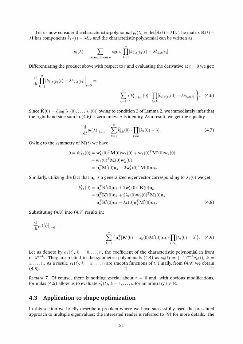
Let us now consider the characteristic polynomial pt(λ) = det[K(t)−λI]. The matrix K(t)−λI has components kk`(t)− λδk` and the characteristic polynomial can be written as
pt(λ) =∑
permutations σ
sgnσ
n∏
k=1
[kk,σ(k)(t)− λδk,σ(k)].
Differentiating the product above with respect to t and evaluating the derivative at t = 0 we get:
d
dt
n∏
k=1
[kk,σ(k)(t)− λδk,σ(k)]
∣∣∣∣t=0
=
n∑
k=1
k′k,σ(k)(0) ·
∏
`6=k[k`,σ(`)(0)− λδ`,σ(`)]
. (4.6)
Since K(0) = diag[λ1(0), . . . , λn(0)] owing to condition 3 of Lemma 2, we immediately infer thatthe right hand side sum in (4.6) is zero unless σ is identity. As a result, we get the equality
d
dtpt(λ)
∣∣t=0
=
n∑
k=1
k′kk(0) ·∏
`6=k[λ`(0)− λ]. (4.7)
Owing to the symmetry of M(t) we have
0 = m′kk(0) = w′k(0)TM(0)wk(0) + wk(0)TM′(0)wk(0)
+ wk(0)TM(0)w′k(0)
= uTkM′(0)uk + 2w′k(0)TM(0)uk.
Similarly, utilizing the fact that uk is a generalized eigenvector corresponding to λk(0) we get
k′kk(0) = uTkK′(0)uk + 2w′k(0)TK(0)uk
= uTkK′(0)uk + 2λk(0)w′k(0)TM(0)uk
= uTkK′(0)uk − λk(0)uTkM′(0)uk. (4.8)
Substituting (4.8) into (4.7) results in:
d
dtpt(λ)
∣∣t=0
=
n∑
k=1
uTk [K′(0)− λk(0)M′(0)]uk ·
∏
`6=k[λ`(0)− λ]
. (4.9)
Let us denote by ak(t), k = 0, . . . , n, the coefficient of the characteristic polynomial in frontof λn−k. They are related to the symmetric polynomials (4.4) as sk(t) = (−1)n−kak(t), k =1, . . . , n. As a result, sk(t), k = 1, . . . , n are smooth functions of t. Finally, from (4.9) we obtain(4.5).
Remark 7. Of course, there is nothing special about t = 0 and, with obvious modifications,formulas (4.5) allow us to evaluate s′k(t), k = 1, . . . , n for an arbitrary t ∈ R.
4.3 Application to shape optimization
In this section we briefly describe a problem where we have successfully used the presentedapproach to multiple eigenvalues; the interested reader is referred to [9] for more details. The
51
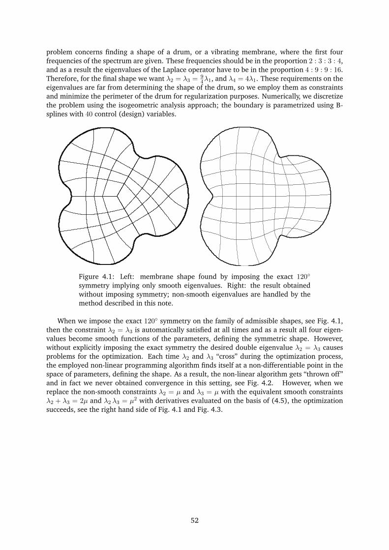
problem concerns finding a shape of a drum, or a vibrating membrane, where the first fourfrequencies of the spectrum are given. These frequencies should be in the proportion 2 : 3 : 3 : 4,and as a result the eigenvalues of the Laplace operator have to be in the proportion 4 : 9 : 9 : 16.Therefore, for the final shape we want λ2 = λ3 = 9
4λ1, and λ4 = 4λ1. These requirements on theeigenvalues are far from determining the shape of the drum, so we employ them as constraintsand minimize the perimeter of the drum for regularization purposes. Numerically, we discretizethe problem using the isogeometric analysis approach; the boundary is parametrized using B-splines with 40 control (design) variables.
Figure 4.1: Left: membrane shape found by imposing the exact 120
symmetry implying only smooth eigenvalues. Right: the result obtainedwithout imposing symmetry; non-smooth eigenvalues are handled by themethod described in this note.
When we impose the exact 120 symmetry on the family of admissible shapes, see Fig. 4.1,then the constraint λ2 = λ3 is automatically satisfied at all times and as a result all four eigen-values become smooth functions of the parameters, defining the symmetric shape. However,without explicitly imposing the exact symmetry the desired double eigenvalue λ2 = λ3 causesproblems for the optimization. Each time λ2 and λ3 “cross” during the optimization process,the employed non-linear programming algorithm finds itself at a non-differentiable point in thespace of parameters, defining the shape. As a result, the non-linear algorithm gets “thrown off”and in fact we never obtained convergence in this setting, see Fig. 4.2. However, when wereplace the non-smooth constraints λ2 = µ and λ3 = µ with the equivalent smooth constraintsλ2 + λ3 = 2µ and λ2 λ3 = µ2 with derivatives evaluated on the basis of (4.5), the optimizationsucceeds, see the right hand side of Fig. 4.1 and Fig. 4.3.
52
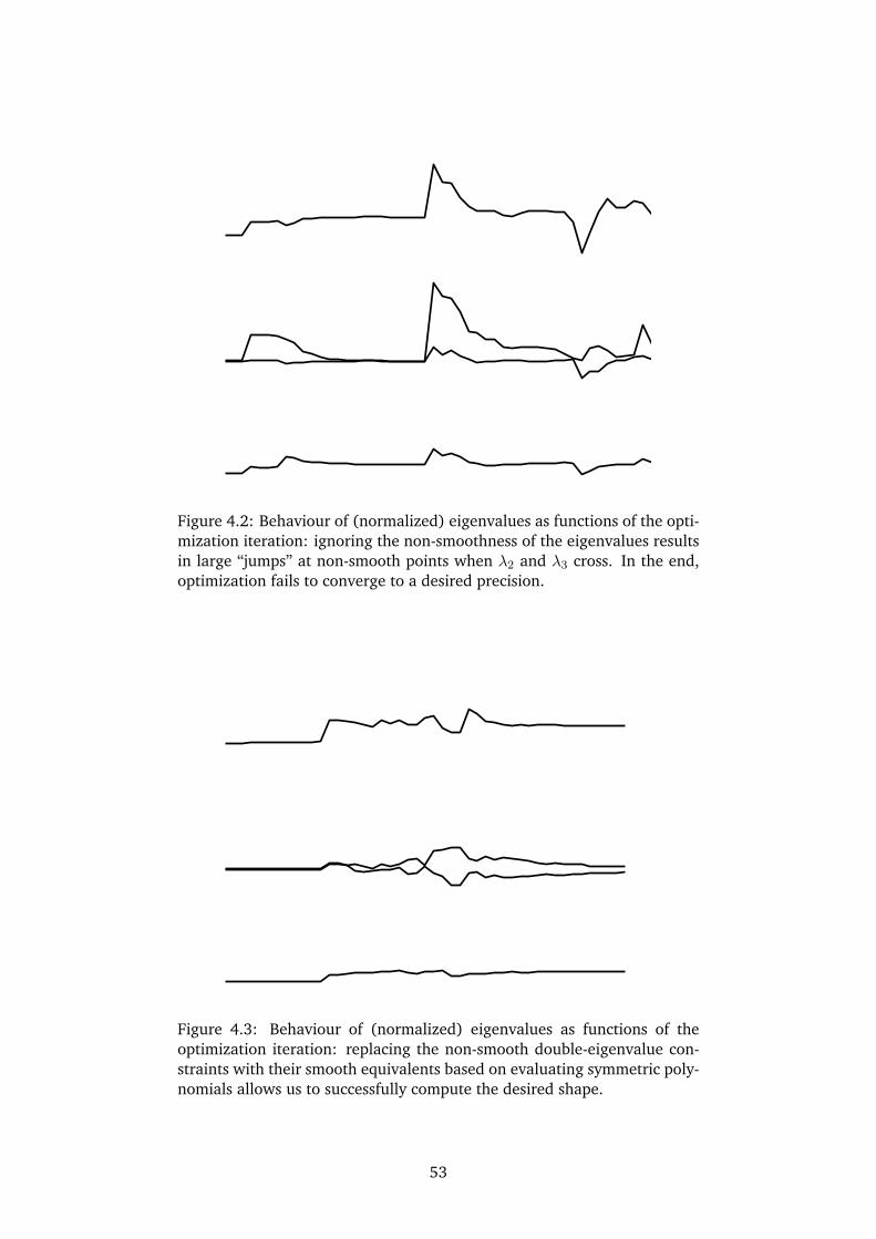
Figure 4.2: Behaviour of (normalized) eigenvalues as functions of the opti-mization iteration: ignoring the non-smoothness of the eigenvalues resultsin large “jumps” at non-smooth points when λ2 and λ3 cross. In the end,optimization fails to converge to a desired precision.
Figure 4.3: Behaviour of (normalized) eigenvalues as functions of theoptimization iteration: replacing the non-smooth double-eigenvalue con-straints with their smooth equivalents based on evaluating symmetric poly-nomials allows us to successfully compute the desired shape.
53

Part III
Shape optimization of sub-wavelengthantennas
55

Chapter 5
Shape optimization of sub-wavelengthantennas using isogeometric analysis
Nguyen D. M., A. Evgrafov, J. Gravesen, Shape optimization of sub-wavelength antenna usingisogeometric analysis, in submission, August, 2011.
Abstract. We consider a problem of designing an antenna that concentrates the magnetic en-ergy of an incoming electromagnetic wave in a small spatial region, having in mind potentialapplications for wireless energy transfer. For this purpose we utilize shape optimization andisogeometric analysis. In order to make such a combination of methods work successfully forthis problem, we propose an inexpensive linear method for re-parametrizing the computationaldomain after each shape update by the optimization algorithm. Our method is based on aquadratic programming approximation of a minimization problem of Winslow functional. Thissimple idea works rather well in our numerical tests. Indeed, we benchmark our shape opti-mization algorithm against earlier attempts of antenna design based on topology optimization,and quite remarkably, our design improves the performance by a factor of one million.
Keywords: shape optimization; isogeometric analysis; spline parametrization; wireless energytransfer; sub-wavelength antennas.
5.1 Introduction
Shape optimization has been a subject of a great interest in the past decades, see for exam-ple [17, 34, 35], and the references therein. Such an interest is fueled by many importantand direct applications of shape optimization in various engineering disciplines, and the subjecthas seen many advances during these years. In this paper, we concentrate on utilizing shapeoptimization techniques to facilitate optimal design of sub-wavelength antennas. As a modelproblem we consider that of focusing the incoming electromagnetic energy into a given smallspatial area, which has immediate applications for wireless energy transfer [64, 65]. Due toa variety of potential industrial applications, such as wireless charging of portable electronicdevices [66] and electric commuter vehicles [67], the problem has attracted a lot of atten-tion. One of the major issues remaining to be resolved is improving the efficiency of the pro-cess [68, 69, 70, 71, 72, 73]. The idea of employing a systematic design procedure such as shapeoptimization for this purpose arises quite naturally.
Many shape optimization approaches continue to rely on polygonal grids inherited from theunderlying numerical methods used for numerical approximation of partial differential equa-tions (PDEs) governing a given physical system under consideration, Maxwell’s equations in our
57
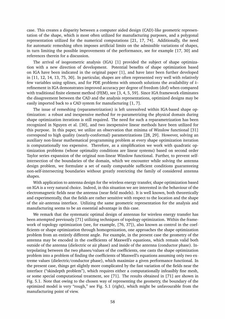
case. This creates a disparity between a computer aided design (CAD)-like geometric represen-tation of the shape, which is most often utilized for manufacturing purposes, and a polygonalrepresentation utilized for the numerical computations [21, 17, 74]. Additionally, the needfor automatic remeshing often imposes artificial limits on the admissible variations of shapes,in turn limiting the possible improvements of the performance, see for example [17, 30] andreferences therein for a discussion.
The arrival of isogeometric analysis (IGA) [1] provided the subject of shape optimiza-tion with a new direction of development. Potential benefits of shape optimization basedon IGA have been indicated in the original paper [1], and have later been further developedin [11, 12, 14, 13, 75, 30]. In particular, shapes are often represented very well with relativelyfew variables using splines, and for PDE problems with smooth solutions the availability of k-refinement in IGA demonstrates improved accuracy per degree of freedom (dof) when comparedwith traditional finite element method (FEM), see [3, 4, 5, 59]. Since IGA framework eliminatesthe disagreement between the CAD and the analysis representations, optimized designs may beeasily imported back to a CAD system for manufacturing [1, 7].
The issue of remeshing (reparametrization) is left unresolved within IGA-based shape op-timization: a robust and inexpensive method for re-parametrizing the physical domain duringshape optimization iterations is still required. The need for such a reparametrization has beenrecognized in Nguyen et al. [30], and two inexpensive linear methods have been utilized forthis purpose. In this paper, we utilize an observation that minima of Winslow functional [31]correspond to high quality (nearly-conformal) parametrizations [28, 29]. However, solving anauxiliary non-linear mathematical programming problem at every shape optimization iterationis computationally too expensive. Therefore, as a simplification we work with quadratic op-timization problems (whose optimality conditions are linear systems) based on second orderTaylor series expansion of the original non-linear Winslow functional. Further, to prevent self-intersection of the boundaries of the domain, which we encounter while solving the antennadesign problem, we formulate a set of easily computable sufficient conditions guaranteeingnon-self-intersecting boundaries without greatly restricting the family of considered antennashapes.
With application to antenna design for the wireless energy transfer, shape optimization basedon IGA is a very natural choice. Indeed, in this situation we are interested in the behaviour of theelectromagnetic fields near the antenna (near field models). It is well known, both theoreticallyand experimentally, that the fields are rather sensitive with respect to the location and the shapeof the air-antenna interface. Utilizing the same geometric representation for the analysis andmanufacturing seems to be an essential advantage in this case.
We remark that the systematic optimal design of antennas for wireless energy transfer hasbeen attempted previously [71] utilizing techniques of topology optimization. Within the frame-work of topology optimization (see, for example, [76, 37]), also known as control in the coef-ficients or shape optimization through homogenization, one approaches the shape optimizationproblem from an entirely different angle. For example, in the present case the geometry of theantenna may be encoded in the coefficients of Maxwell’s equations, which remain valid bothoutside of the antenna (dielectric or air phase) and inside of the antenna (conductor phase). In-terpolating between the two phases/values of the coefficients, one casts the shape optimizationproblem into a problem of finding the coefficients of Maxwell’s equations assuming only two ex-treme values (dielectric/conductor phase), which maximize a given performance functional. Inthe present case, things get slightly more complicated by the fast variation of the fields near theinterface (“skindepth problem”), which requires either a computationally infeasibly fine mesh,or some special computational treatment, see [71]. The results obtained in [71] are shown inFig. 5.1. Note that owing to the chosen way of representing the geometry, the boundary of theoptimized model is very “rough,” see Fig. 5.1 (right), which might be unfavourable from themanufacturing point of view.
58
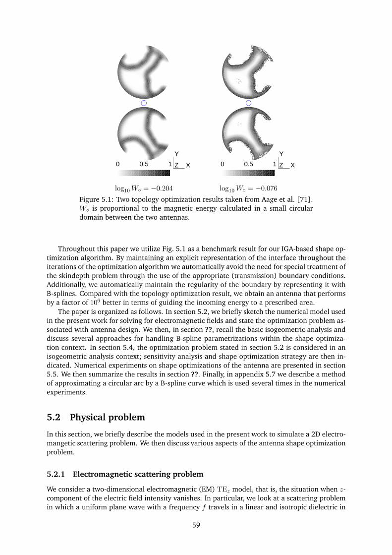
0 0.5 1
Y
XZ 0 0.5 1
Y
XZ
log10W = −0.204 log10W = −0.076
g g
Figure 5.1: Two topology optimization results taken from Aage et al. [71].W is proportional to the magnetic energy calculated in a small circulardomain between the two antennas.
Throughout this paper we utilize Fig. 5.1 as a benchmark result for our IGA-based shape op-timization algorithm. By maintaining an explicit representation of the interface throughout theiterations of the optimization algorithm we automatically avoid the need for special treatment ofthe skindepth problem through the use of the appropriate (transmission) boundary conditions.Additionally, we automatically maintain the regularity of the boundary by representing it withB-splines. Compared with the topology optimization result, we obtain an antenna that performsby a factor of 106 better in terms of guiding the incoming energy to a prescribed area.
The paper is organized as follows. In section 5.2, we briefly sketch the numerical model usedin the present work for solving for electromagnetic fields and state the optimization problem as-sociated with antenna design. We then, in section ??, recall the basic isogeometric analysis anddiscuss several approaches for handling B-spline parametrizations within the shape optimiza-tion context. In section 5.4, the optimization problem stated in section 5.2 is considered in anisogeometric analysis context; sensitivity analysis and shape optimization strategy are then in-dicated. Numerical experiments on shape optimizations of the antenna are presented in section5.5. We then summarize the results in section ??. Finally, in appendix 5.7 we describe a methodof approximating a circular arc by a B-spline curve which is used several times in the numericalexperiments.
5.2 Physical problem
In this section, we briefly describe the models used in the present work to simulate a 2D electro-mangetic scattering problem. We then discuss various aspects of the antenna shape optimizationproblem.
5.2.1 Electromagnetic scattering problem
We consider a two-dimensional electromagnetic (EM) TEz model, that is, the situation when z-component of the electric field intensity vanishes. In particular, we look at a scattering problemin which a uniform plane wave with a frequency f travels in a linear and isotropic dielectric in
59
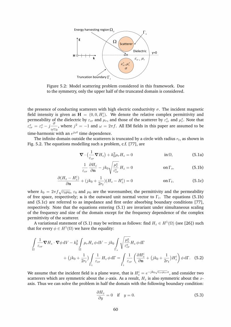
Scatterer
Energy harvesting region
k H
E
.
Truncation boundary
Dielectric
crε , rµ
,s scr rε µ
Ω
sΓ
tΓ
Ω
y=0
σ
Figure 5.2: Model scattering problem considered in this framework. Dueto the symmetry, only the upper half of the truncated domain is considered.
the presence of conducting scatterers with high electric conductivity σ. The incident magneticfield intensity is given as H = (0, 0, H i
z). We denote the relative complex permittivity andpermeability of the dielectric by εcr and µr, and those of the scatterer by εscr and µsr. Note thatεscr = εsr − j
σ
ωε0, where j2 = −1 and ω = 2πf . All EM fields in this paper are assumed to be
time-harmonic with an ejωt time dependence.The infinite domain outside the scatterers is truncated by a circle with radius rt, as shown in
Fig. 5.2. The equations modelling such a problem, c.f. [77], are
∇ ·( 1
εcr∇Hz
)+ k2
0µrHz = 0 in Ω, (5.1a)
1
εcr
∂Hz
∂n− jk0
õsr
εscr
Hz = 0 on Γs, (5.1b)
∂(Hz −H iz)
∂n+ (jk0 +
1
2rt)(Hz −H i
z) = 0 on Γt, (5.1c)
where k0 = 2πf√ε0µ0, ε0 and µ0 are the wavenumber, the permittivity and the permeability
of free space, respectively; n is the outward unit normal vector to Γt. The equations (5.1b)and (5.1c) are referred to as impedance and first order absorbing boundary conditions [77],respectively. Note that the equations entering (5.1) are invariant under simultaneous scalingof the frequency and size of the domain except for the frequency dependence of the complexpermittivity of the scatterer.
A variational statement of (5.1) may be written as follows: find Hz ∈ H1(Ω) (see [26]) suchthat for every φ ∈ H1(Ω) we have the equality:
∫
Ω
1
εcr∇Hz ·∇φ dV − k2
0
∫
Ω
µrHz φ dV − jk0
∫
Γs
õsr
εscr
Hz φ dΓ
+(jk0 +
1
2rt
) ∫
Γt
1
εcrHz φ dΓ =
∫
Γt
1
εcr
(∂H i
z
∂n+(jk0 +
1
2rt
)H iz
)φ dΓ. (5.2)
We assume that the incident field is a plane wave, that is H iz = e−jk0
√εcrµcrx, and consider two
scatterers which are symmetric about the x-axis. As a result, Hz is also symmetric about the x-axis. Thus we can solve the problem in half the domain with the following boundary condition:
∂Hz
∂y= 0 if y = 0. (5.3)
60
Figure 5.3: An optimization result in which no regularity conditions areimposed. Note that the boundary of the antenna approaches the truncationboundaries and also self-intersects.
5.2.2 Shape optimization problem
We consider the problem of finding shapes of antennas depicted in Fig. 5.2 in order to maximizethe following quantity, which is proportional to the magnetic energy
W = 2
∫
Ω
|Hz|2 dV (5.4)
where Hz is the solution to the equations (5.1). The domain Ω in (5.4) is a relatively smallregion of space between the two antennas, see in Fig. 5.2. In (5.4), the factor 2 accounts forthe fact that we integrate only over a half of a symmetric domain. The only difference betweenthe problem studied in Aage et al. [71] and the one studied in this paper is that we maximizemagnetic energy in a small rectangular region and not in a small circular region. However, inorder to compare the efficiency of our antenna design with the one found in Aage et al. [71] welater evaluate the magnetic energy in the circular region as well.
We now look at whether and which regularization conditions and/or constraints are neededfor this problem. Having applications for wireless energy transfers in mind, a space betweenthe two antennas is needed for placing an energy harvesting device. Therefore, it is necessaryto introduce a lower bound on the position of the antenna guaranteeing the existence of sucha space. We also observe that, unless prevented from doing so the resonator tends to growwithout bound and its boundary tends to self-intersect, see Fig. 5.3. Therefore, we also introducean upper bound on resonator’s volume and a set of conditions to prevent the shape from self-intersecting.
5.3 Isogeometric analysis
In this section we recall the basic two-dimensional B-spline based isogeometric analysis (IGA).Similarly to the standard FEM, the underlying principle of IGA is the use of the Galerkinmethod [2]. Thus we approximate a weak solution to a given boundary value problem asso-ciated with Maxwell’s equations in a finite-dimensional space spanned by certain basis (shape)functions. In the present case, the basis functions are defined indirectly via a spline parametriza-tion of the physical domain and bivariate B-spline tensor products in the parameter domain[0, 1]2.
61
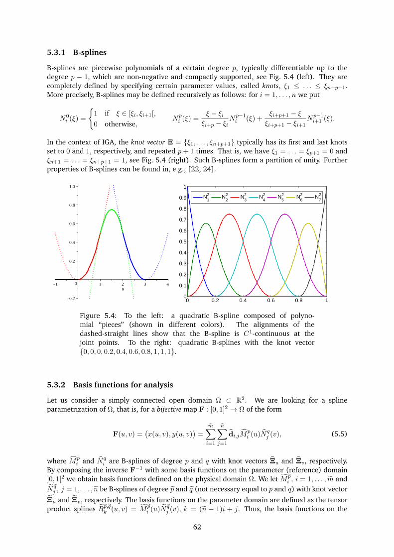
5.3.1 B-splines
B-splines are piecewise polynomials of a certain degree p, typically differentiable up to thedegree p − 1, which are non-negative and compactly supported, see Fig. 5.4 (left). They arecompletely defined by specifying certain parameter values, called knots, ξ1 ≤ . . . ≤ ξn+p+1.More precisely, B-splines may be defined recursively as follows: for i = 1, . . . , n we put
N0i (ξ) =
1 if ξ ∈ [ξi, ξi+1[,
0 otherwise,Npi (ξ) =
ξ − ξiξi+p − ξi
Np−1i (ξ) +
ξi+p+1 − ξξi+p+1 − ξi+1
Np−1i+1 (ξ).
In the context of IGA, the knot vector Ξ = ξ1, . . . , ξn+p+1 typically has its first and last knotsset to 0 and 1, respectively, and repeated p+ 1 times. That is, we have ξ1 = . . . = ξp+1 = 0 andξn+1 = . . . = ξn+p+1 = 1, see Fig. 5.4 (right). Such B-splines form a partition of unity. Furtherproperties of B-splines can be found in, e.g., [22, 24].
0 0.2 0.4 0.6 0.8 10
0.1
0.2
0.3
0.4
0.5
0.6
0.7
0.8
0.9
1
N21
N22
N23
N24
N25
N26
N27
Figure 5.4: To the left: a quadratic B-spline composed of polyno-mial “pieces” (shown in different colors). The alignments of thedashed-straight lines show that the B-spline is C1-continuous at thejoint points. To the right: quadratic B-splines with the knot vector0, 0, 0, 0.2, 0.4, 0.6, 0.8, 1, 1, 1.
5.3.2 Basis functions for analysis
Let us consider a simply connected open domain Ω ⊂ R2. We are looking for a splineparametrization of Ω, that is, for a bijective map F : [0, 1]2 → Ω of the form
F(u, v) =(x(u, v), y(u, v)
)=
m∑
i=1
n∑
j=1
di,jMpi (u)N q
j (v), (5.5)
where Mpi and N q
i are B-splines of degree p and q with knot vectors Ξu and Ξv, respectively.By composing the inverse F−1 with some basis functions on the parameter (reference) domain]0, 1[2 we obtain basis functions defined on the physical domain Ω. We let M p
i , i = 1, . . . , m andN qj , j = 1, . . . , n be B-splines of degree p and q (not necessary equal to p and q) with knot vector
Ξu and Ξv, respectively. The basis functions on the parameter domain are defined as the tensorproduct splines Rp,qk (u, v) = M p
i (u)N qj (v), k = (n − 1)i + j. Thus, the basis functions on the
62
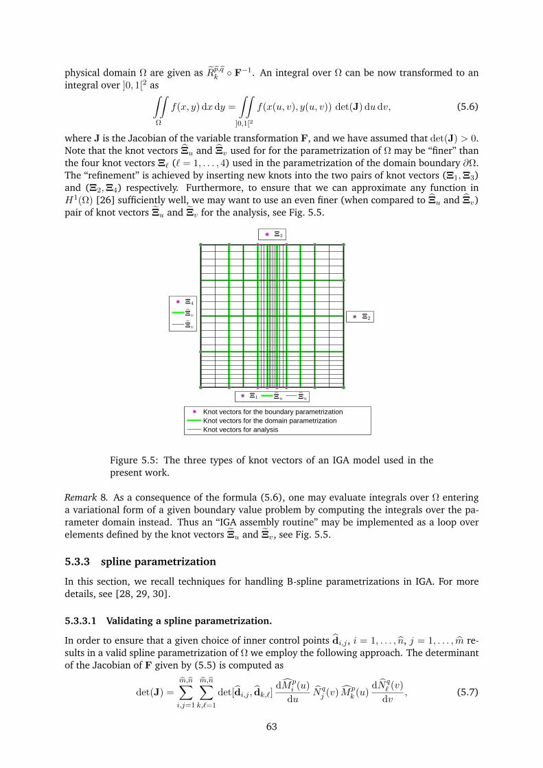
physical domain Ω are given as Rp,qk F−1. An integral over Ω can be now transformed to anintegral over ]0, 1[2 as
∫∫
Ω
f(x, y) dx dy =
∫∫
]0,1[2
f(x(u, v), y(u, v)) det(J) dudv, (5.6)
where J is the Jacobian of the variable transformation F, and we have assumed that det(J) > 0.Note that the knot vectors Ξu and Ξv used for for the parametrization of Ω may be “finer” thanthe four knot vectors Ξ` (` = 1, . . . , 4) used in the parametrization of the domain boundary ∂Ω.The “refinement” is achieved by inserting new knots into the two pairs of knot vectors (Ξ1,Ξ3)and (Ξ2,Ξ4) respectively. Furthermore, to ensure that we can approximate any function inH1(Ω) [26] sufficiently well, we may want to use an even finer (when compared to Ξu and Ξv)pair of knot vectors Ξu and Ξv for the analysis, see Fig. 5.5.
Ξ1 Ξu Ξu
Ξ3
Ξ2
Ξ4
Ξv
Ξv
Knot vectors for the boundary parametrizationKnot vectors for the domain parametrizationKnot vectors for analysis
Figure 5.5: The three types of knot vectors of an IGA model used in thepresent work.
Remark 8. As a consequence of the formula (5.6), one may evaluate integrals over Ω enteringa variational form of a given boundary value problem by computing the integrals over the pa-rameter domain instead. Thus an “IGA assembly routine” may be implemented as a loop overelements defined by the knot vectors Ξu and Ξv, see Fig. 5.5.
5.3.3 spline parametrization
In this section, we recall techniques for handling B-spline parametrizations in IGA. For moredetails, see [28, 29, 30].
5.3.3.1 Validating a spline parametrization.
In order to ensure that a given choice of inner control points di,j , i = 1, . . . , n, j = 1, . . . , m re-sults in a valid spline parametrization of Ω we employ the following approach. The determinantof the Jacobian of F given by (5.5) is computed as
det(J) =
m,n∑
i,j=1
m,n∑
k,`=1
det[di,j , dk,`]dMp
i (u)
duN qj (v) Mp
k (u)dN q
` (v)
dv, (5.7)
63
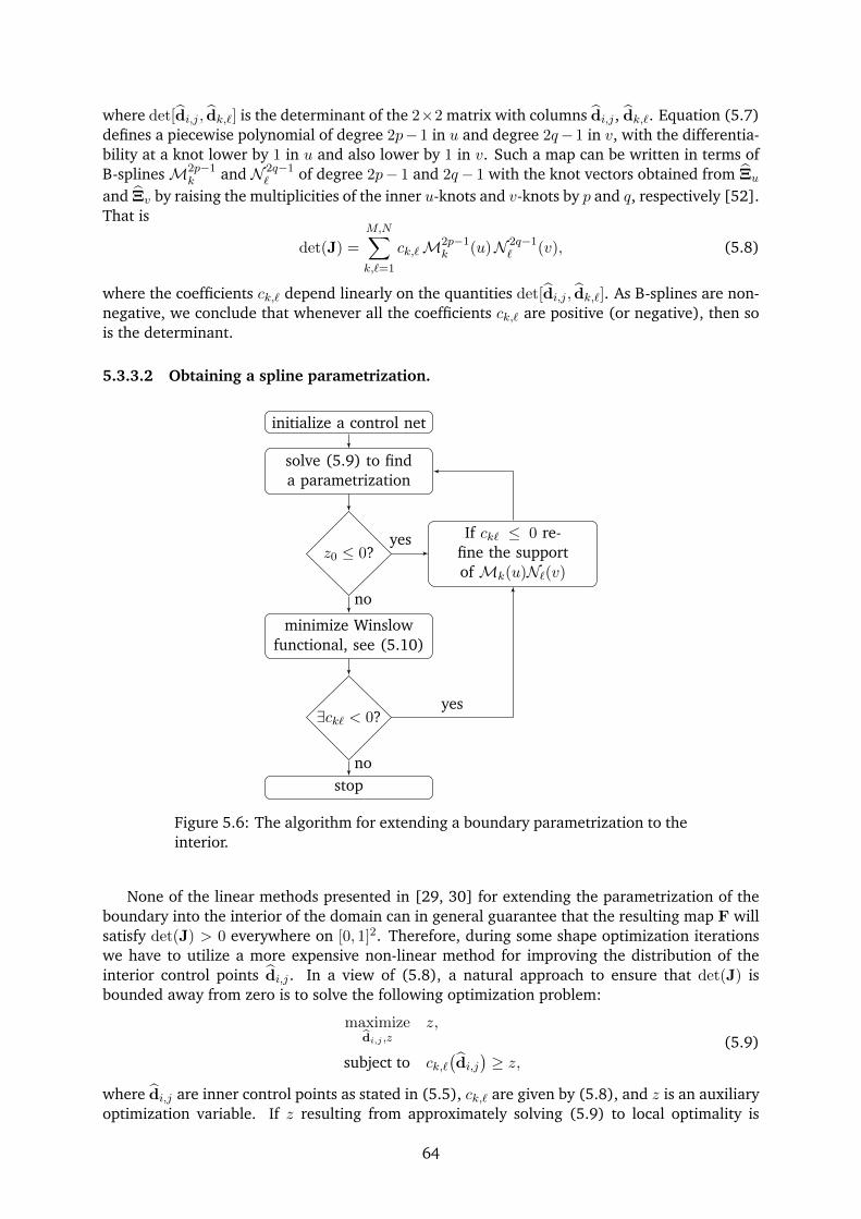
where det[di,j , dk,`] is the determinant of the 2×2 matrix with columns di,j , dk,`. Equation (5.7)defines a piecewise polynomial of degree 2p−1 in u and degree 2q−1 in v, with the differentia-bility at a knot lower by 1 in u and also lower by 1 in v. Such a map can be written in terms ofB-splinesM2p−1
k and N 2q−1` of degree 2p− 1 and 2q− 1 with the knot vectors obtained from Ξu
and Ξv by raising the multiplicities of the inner u-knots and v-knots by p and q, respectively [52].That is
det(J) =
M,N∑
k,`=1
ck,`M2p−1k (u)N 2q−1
` (v), (5.8)
where the coefficients ck,` depend linearly on the quantities det[di,j , dk,`]. As B-splines are non-negative, we conclude that whenever all the coefficients ck,` are positive (or negative), then sois the determinant.
5.3.3.2 Obtaining a spline parametrization.
initialize a control net
solve (5.9) to finda parametrization
z0 ≤ 0?
minimize Winslowfunctional, see (5.10)
If ck` ≤ 0 re-fine the supportof Mk(u)N`(v)
∃ck` < 0?
stop
yes
no
yes
no
Figure 5.6: The algorithm for extending a boundary parametrization to theinterior.
None of the linear methods presented in [29, 30] for extending the parametrization of theboundary into the interior of the domain can in general guarantee that the resulting map F willsatisfy det(J) > 0 everywhere on [0, 1]2. Therefore, during some shape optimization iterationswe have to utilize a more expensive non-linear method for improving the distribution of theinterior control points di,j . In a view of (5.8), a natural approach to ensure that det(J) isbounded away from zero is to solve the following optimization problem:
maximizedi,j ,z
z,
subject to ck,`(di,j)≥ z,
(5.9)
where di,j are inner control points as stated in (5.5), ck,` are given by (5.8), and z is an auxiliaryoptimization variable. If z resulting from approximately solving (5.9) to local optimality is
64
positive then we are guaranteed to have a valid parametrization. Unfortunately, the quality ofthe parametrization obtained in this fashion needs not to be very high. Thus, we improve theparametrization by looking at the following constrained optimization problem:
minimizeinner control points di,j
∫ 1
0
∫ 1
0W (di,j) dudv,
subject to ck`(di,j)≥ δz0
(5.10)
where W (di,j) = (‖Fu‖2 + ‖Fv‖2)/ det[Fu,Fv] is referred to as the Winslow functional [31].In (5.10), z0 > 0 is computed by approximately solving (5.9) and δ ∈ [0, 1] is a fixed relaxationparameter.
In our numerical experiments we utilize the interior point algorithm constituting a part ofOptimization Framework in Matlab [33] for solving the optimization problems (5.9) and (5.10)to approximate stationarity. Also, we set δ = 0 in (5.10). The whole process is outlined inFig. 5.6.
5.3.3.3 Linearized Winslow functional.
The algorithm for finding a valid domain parametrization described above has to be carriedout at every iteration of an “outer” shape optimization algorithm. Firstly, this process is rathercomputationally expensive, as it requires solving two non-linear programming problems at ev-ery shape optimization iteration. Secondly, as we solve the said optimization problems onlyapproximately, it is not possible to find the derivatives of the inner control points with respectto changes of boundary control points. The latter does not allow us to use gradient based opti-mization algorithms for the “outer” shape optimization problem.
To avoid this difficulty, we linearize the process of computing a domain parametrization.Namely, we can Taylor-expand the Winslow functional as
W(d) =
∫∫
ΩW (d) dudv ≈ W(d0) + (d− d0)T G(d0) +
1
2(d− d0)T H(d0) (d− d0), (5.11)
where d is a vector with all control points di,j , d0 is the control points for a referenceparametrization obtained by solving (5.10), and G and H are the gradient and Hessian ofW re-spectively. If we split the control points d = (d1 d2)T into the part d2 that is given (typically theboundary control points) and the part d1 that has to be determined (typically the inner controlpoints), then we can write (5.11) as
W(d) ≈ W(d0) +(d1 − d1,0 d2 − d2,0
)(G1
G2
)
+1
2
(d1 − d1,0 d2 − d2,0
)(H11 H12
H21 H22
)(d1 − d1,0
d2 − d2,0
). (5.12)
The minimum of the right hand side of (5.12) is obtained when d1 satisfies the linear equation
H11(d1 − d1,0) = −G1 −H12(d2 − d2,0). (5.13)
This gives us a fast method for computing the domain parametrization and its derivativeswith respect to the boundary control points. We use this method as long as we obtain avalid parametrization, but if the parametrization at some point fails the test described in Sec-tion 5.3.3.1 then we restart the “outer” shape optimization algorithm with a new referenceparametrization d0 found by the method described in Section 5.3.3.2.
The given control points d2 can further be split into the set of fixed control points df andcontrol points Rd obtained from the design variables (control points) d by knot insertion (re-finement).
65
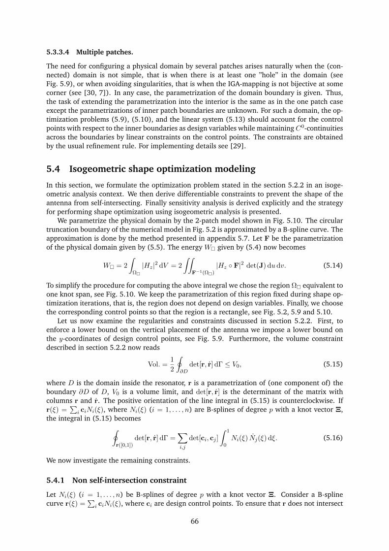
5.3.3.4 Multiple patches.
The need for configuring a physical domain by several patches arises naturally when the (con-nected) domain is not simple, that is when there is at least one ”hole” in the domain (seeFig. 5.9), or when avoiding singularities, that is when the IGA-mapping is not bijective at somecorner (see [30, 7]). In any case, the parametrization of the domain boundary is given. Thus,the task of extending the parametrization into the interior is the same as in the one patch caseexcept the parametrizations of inner patch boundaries are unknown. For such a domain, the op-timization problems (5.9), (5.10), and the linear system (5.13) should account for the controlpoints with respect to the inner boundaries as design variables while maintaining C0-continuitiesacross the boundaries by linear constraints on the control points. The constraints are obtainedby the usual refinement rule. For implementing details see [29].
5.4 Isogeometric shape optimization modeling
In this section, we formulate the optimization problem stated in the section 5.2.2 in an isoge-ometric analysis context. We then derive differentiable constraints to prevent the shape of theantenna from self-intersecting. Finally sensitivity analysis is derived explicitly and the strategyfor performing shape optimization using isogeometric analysis is presented.
We parametrize the physical domain by the 2-patch model shown in Fig. 5.10. The circulartruncation boundary of the numerical model in Fig. 5.2 is approximated by a B-spline curve. Theapproximation is done by the method presented in appendix 5.7. Let F be the parametrizationof the physical domain given by (5.5). The energy W given by (5.4) now becomes
W = 2
∫
Ω
|Hz|2 dV = 2
∫∫
F−1(Ω)|Hz F|2 det(J) dudv. (5.14)
To simplify the procedure for computing the above integral we chose the region Ω equivalent toone knot span, see Fig. 5.10. We keep the parametrization of this region fixed during shape op-timization iterations, that is, the region does not depend on design variables. Finally, we choosethe corresponding control points so that the region is a rectangle, see Fig. 5.2, 5.9 and 5.10.
Let us now examine the regularities and constraints discussed in section 5.2.2. First, toenforce a lower bound on the vertical placement of the antenna we impose a lower bound onthe y-coordinates of design control points, see Fig. 5.9. Furthermore, the volume constraintdescribed in section 5.2.2 now reads
Vol. =1
2
∮
∂Ddet[r, r] dΓ ≤ V0, (5.15)
where D is the domain inside the resonator, r is a parametrization of (one component of) theboundary ∂D of D, V0 is a volume limit, and det[r, r] is the determinant of the matrix withcolumns r and r. The positive orientation of the line integral in (5.15) is counterclockwise. Ifr(ξ) =
∑i ciNi(ξ), where Ni(ξ) (i = 1, . . . , n) are B-splines of degree p with a knot vector Ξ,
the integral in (5.15) becomes∮
r([0,1])det[r, r] dΓ =
∑
i,j
det[ci, cj ]
∫ 1
0Ni(ξ) Nj(ξ) dξ. (5.16)
We now investigate the remaining constraints.
5.4.1 Non self-intersection constraint
Let Ni(ξ) (i = 1, . . . , n) be B-splines of degree p with a knot vector Ξ. Consider a B-splinecurve r(ξ) =
∑i ciNi(ξ), where ci are design control points. To ensure that r does not intersect
66
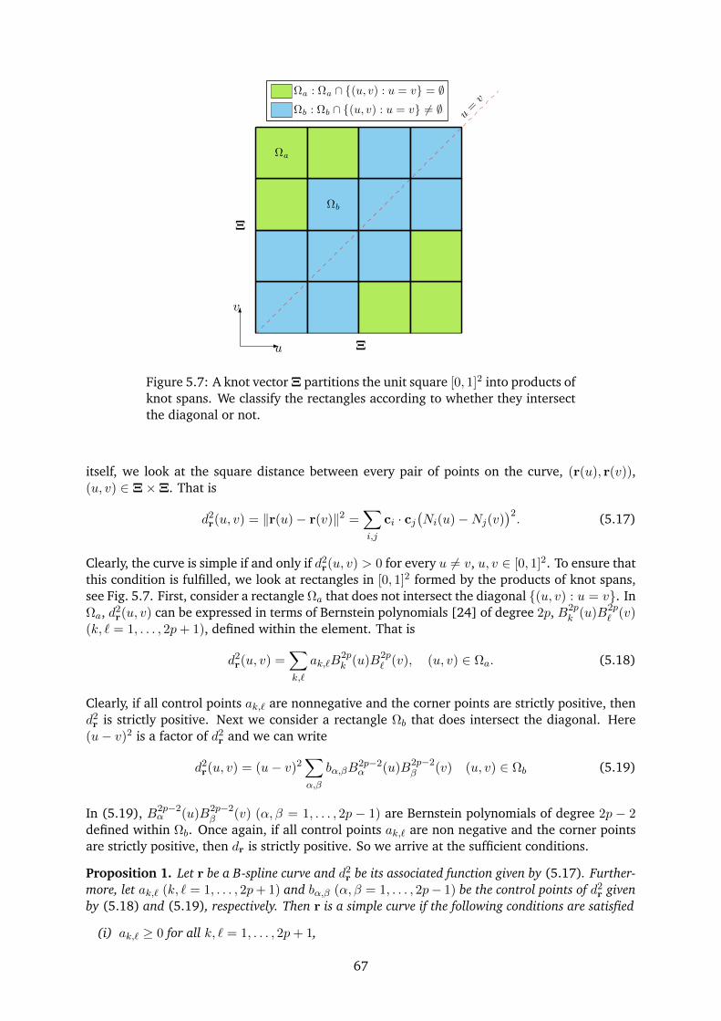
u=v
Ωa
Ωb
Ωa : Ωa ∩ (u, v) : u = v = ∅Ωb : Ωb ∩ (u, v) : u = v 6= ∅
-
6
u
v
Ξ
Ξ
Figure 5.7: A knot vector Ξ partitions the unit square [0, 1]2 into products ofknot spans. We classify the rectangles according to whether they intersectthe diagonal or not.
itself, we look at the square distance between every pair of points on the curve, (r(u), r(v)),(u, v) ∈ Ξ×Ξ. That is
d2r(u, v) = ‖r(u)− r(v)‖2 =
∑
i,j
ci · cj(Ni(u)−Nj(v)
)2. (5.17)
Clearly, the curve is simple if and only if d2r(u, v) > 0 for every u 6= v, u, v ∈ [0, 1]2. To ensure that
this condition is fulfilled, we look at rectangles in [0, 1]2 formed by the products of knot spans,see Fig. 5.7. First, consider a rectangle Ωa that does not intersect the diagonal (u, v) : u = v. InΩa, d2
r(u, v) can be expressed in terms of Bernstein polynomials [24] of degree 2p, B2pk (u)B2p
` (v)(k, ` = 1, . . . , 2p+ 1), defined within the element. That is
d2r(u, v) =
∑
k,`
ak,`B2pk (u)B2p
` (v), (u, v) ∈ Ωa. (5.18)
Clearly, if all control points ak,` are nonnegative and the corner points are strictly positive, thend2r is strictly positive. Next we consider a rectangle Ωb that does intersect the diagonal. Here
(u− v)2 is a factor of d2r and we can write
d2r(u, v) = (u− v)2
∑
α,β
bα,βB2p−2α (u)B2p−2
β (v) (u, v) ∈ Ωb (5.19)
In (5.19), B2p−2α (u)B2p−2
β (v) (α, β = 1, . . . , 2p − 1) are Bernstein polynomials of degree 2p − 2defined within Ωb. Once again, if all control points ak,` are non negative and the corner pointsare strictly positive, then dr is strictly positive. So we arrive at the sufficient conditions.
Proposition 1. Let r be a B-spline curve and d2r be its associated function given by (5.17). Further-
more, let ak,` (k, ` = 1, . . . , 2p+ 1) and bα,β (α, β = 1, . . . , 2p− 1) be the control points of d2r given
by (5.18) and (5.19), respectively. Then r is a simple curve if the following conditions are satisfied
(i) ak,` ≥ 0 for all k, ` = 1, . . . , 2p+ 1,
67
(ii) bα,β ≥ 0 for all α, β = 1, . . . , 2p− 1,
(iii) d2r(ξi, ξj) ≥ δ, i, j = 1, . . . , n, for some positive δ.
Note that utilizing the symmetry in (5.17) about the line u = v, only one half of the con-ditions are needed. Also, similarly to (5.31), the coefficients ak,` in (5.18) and bα,β in (5.19)may be explicitly represented as quadratic forms of the design control points ci. For the currentoptimization problem, the antenna boundary is composed of two B-spline curves. Proposition 1can be straightforwardly extended to a piecewise B-spline curve. Finally, knot insertions may beneeded in order to obtain tighter conditions for the sufficiency.
5.4.2 Discretization
An approximation to the solution Hz to (5.1) is expanded in terms of the basis functions (seeSection 5.3.2) as Hz =
∑k hk (Rp,qk F−1) =
[Rp,q1 F−1, . . . , Rp,qmn F−1
]h, where h contains
all the coordinates of Hz with respect to the selected basis. Substituting this expression into theweak form (??) and utilizing the basis functions as the test functions, we arrive at the followingset of linear algebraic equations:
(K + M + S + T) h = f . (5.20)
Entries of the matrices entering (5.20) are with the help of (5.6) calculated as:
Kk` =
∫∫
[0,1]2
1
εcr
(DRp,qk (u, v) J−1
)TDRp,q` (u, v) J−1 det(J) dudv, (5.21a)
Mk` = −k20
∫∫
[0,1]2
µr Rp,qk (u, v) Rp,q` (u, v) det(J) dudv, (5.21b)
Sk` = −jk0
∫
F−1(Γs)
µsrεscr
Rp,qk (u, v) Rp,q` (u, v) ds, (5.21c)
Tk` =(jk0 +
1
2rt
) ∫
F−1(Γt)
1
εcrRp,qk (u, v) Rp,q` (u, v) ds, (5.21d)
f` =
∫
F−1(Γt)
1
εcr
(∂H i
z
∂n+(jk0 +
1
2rt
)H iz
)Rp,q` (u, v) ds, (5.21e)
k, ` = 1, . . . , mn. In the equations (5.21), J is the Jacobian of the parametrization F andDf(u, v) =
[∂f∂u(u, v) ∂f
∂v (u, v)]
is the differential of a real-valued function f : [0, 1]2 → R.
5.4.3 Formulation of the optimization problem and sensitivity analysis
Recall that d is the vector containing components of design control points, see Fig. 5.9.Taking the constraints discussed above into account and noting that in (5.14), Hz F =[Rp,q1 , . . . , Rp,qmn
]h, we arrive at the following shape optimization problem:
maximized∈RN
log10(W) = log10
(2
∫∫
F−1(Ω)
∣∣[Rp,q1 , . . . , Rp,qmn]h∣∣2 det(J) dudv
), (5.22a)
such that yd ≥ y0, (5.22b)
Vol. =1
2
∮
∂Ddet(r, r) dΓ ≤ V0, (5.22c)
ak,` ≥ 0, bα,β ≥ 0, d2r(ξi, ξj) ≥ δ, (c.f. proposition 1) (5.22d)
(K + M + S + T) h = f , (5.22e)
68
where yd are the y-coordinates of the design control points, and y0 is a lower bound.Let us now find first order derivatives of functions involved in (5.22). First, consider the
constraints (5.22d). As noted in subsection 5.4.1 the quantities ak,`, bα,β, and dr(ξi, ξj) in (i−iii)of Proposition 1 are quadratic forms of the design control point vector d, therefore evaluatingtheir gradients with respect to d is a straightforward calculation. The same holds for (5.22c)owing to (5.16). On the other hand, the objective function in (5.22) depends implicitly on dthrough the discretized Maxwell’s equations (5.22e). Consider the partial derivative of W withrespect to a component di of d. Rewriting (5.14) asW = 2
∫∫F−1(Ω)HzFHz F det(J) dudv,
and noting that F−1(Ω) and consequently J∣∣F−1(Ω)
is independent from di, we have
∂W
∂di= 4
∫∫
F−1(Ω)Re
(∂(Hz F)
diHz F
)det(J) dudv. (5.23)
Since we clearly have∂(Hz F)
di=[Rp,q1 , . . . , Rp,qmn
]∂h
di, (5.24)
it remains to determine ∂hdi
. Differentiating the two sides of (5.20) and utilizing the fact that∂Tdi
= ∂fdi
= 0, the partial derivative is in turn the solution to the following linear system
(K + M + S + T)∂h
di= −∂(K + M + S)
dih. (5.25)
In (5.25), the partial derivatives of K, M, and S are calculated straightforwardly by differ-entiating (5.21). Finally, as we employ a linear parametrization method discussed in Subsec-tion 5.3.3.3, d is an affine function of d. That is
d = Ad + B, (5.26)
where the matrices A and B can be explicitly determined from (2.13). Note that the refine-ment matrices [24] obtained when inserting knots into the boundary knot vectors to haveparametrization knot vectors are already taken into account in A. Therefore, the desired sensi-tivities are
∂W
∂d= AT∂W
∂d. (5.27)
5.4.4 Shape optimization strategy
The optimization strategy is outlined in Fig. 5.8. It should be noted that the step “make smalleroptimization step” is inefficient if the number of design variables is relatively large. Neverthe-less, within isogeometric shape optimization we usually have relatively small number of designvariables, and consequently the relative computational cost of such a step is tolerable. Also, bythe step “update analysis and truncation boundar” the correctness of solution as well as trunca-tion boundary approximation is improved towards the end of optimization.
Let us now elaborate on a few steps in the diagram in Fig. 5.8. Verifying whether “thecurrent parametrization is valid” is done by dividing every knot interval of the parametrizationknot vectors uniformly N times. The parametrization is valid if all the control points in (5.8)satisfy the inequalities ck,` ≥ δc, and det(J)(at Gaussian net) ≥ δJ, where δc and δJ are smallnumbers relatively to the volume of the checked patch. Finally, in the step “n times in a row,”one could alternatively check whether the magnitude of the stepsize from the current designvariables to that of the reference parametrization exceeds a given parameter.
69
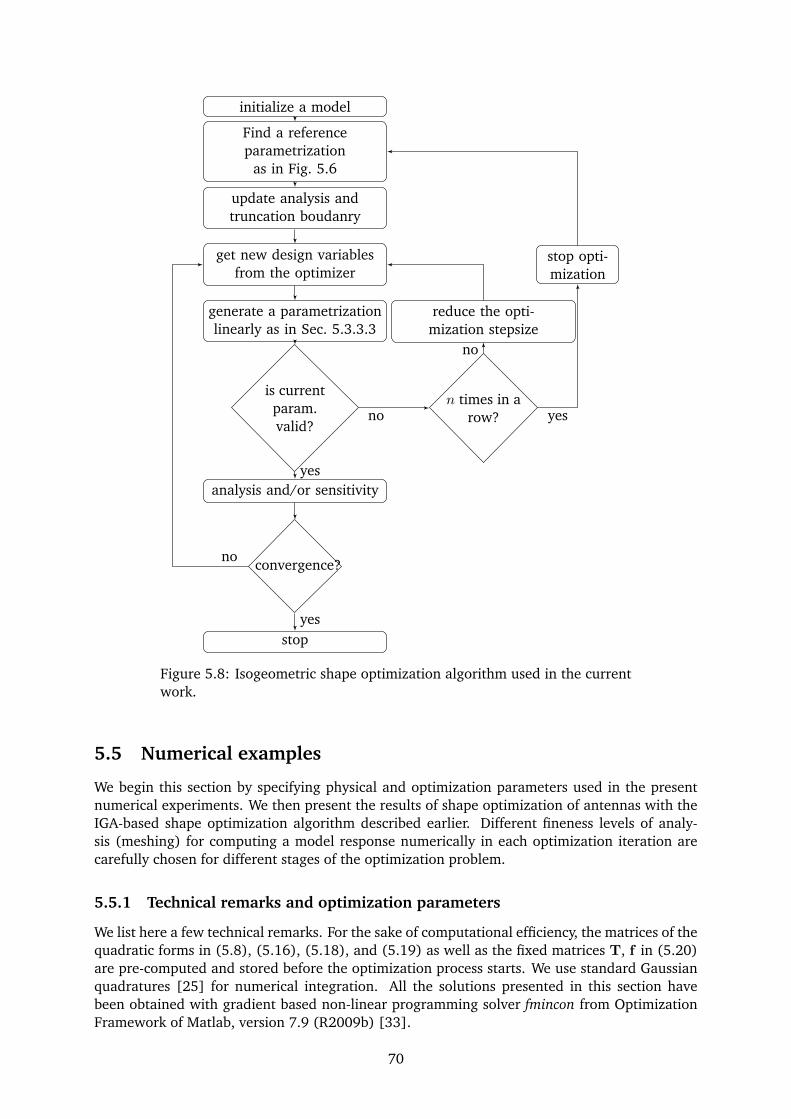
initialize a model
Find a referenceparametrization
as in Fig. 5.6
update analysis andtruncation boudanry
get new design variablesfrom the optimizer
generate a parametrizationlinearly as in Sec. 5.3.3.3
is currentparam.valid?
reduce the opti-mization stepsize
n times in arow?
stop opti-mization
analysis and/or sensitivity
convergence?
stop
yes
no
no
yes
yes
no
Figure 5.8: Isogeometric shape optimization algorithm used in the currentwork.
5.5 Numerical examples
We begin this section by specifying physical and optimization parameters used in the presentnumerical experiments. We then present the results of shape optimization of antennas with theIGA-based shape optimization algorithm described earlier. Different fineness levels of analy-sis (meshing) for computing a model response numerically in each optimization iteration arecarefully chosen for different stages of the optimization problem.
5.5.1 Technical remarks and optimization parameters
We list here a few technical remarks. For the sake of computational efficiency, the matrices of thequadratic forms in (5.8), (5.16), (5.18), and (5.19) as well as the fixed matrices T, f in (5.20)are pre-computed and stored before the optimization process starts. We use standard Gaussianquadratures [25] for numerical integration. All the solutions presented in this section havebeen obtained with gradient based non-linear programming solver fmincon from OptimizationFramework of Matlab, version 7.9 (R2009b) [33].
70
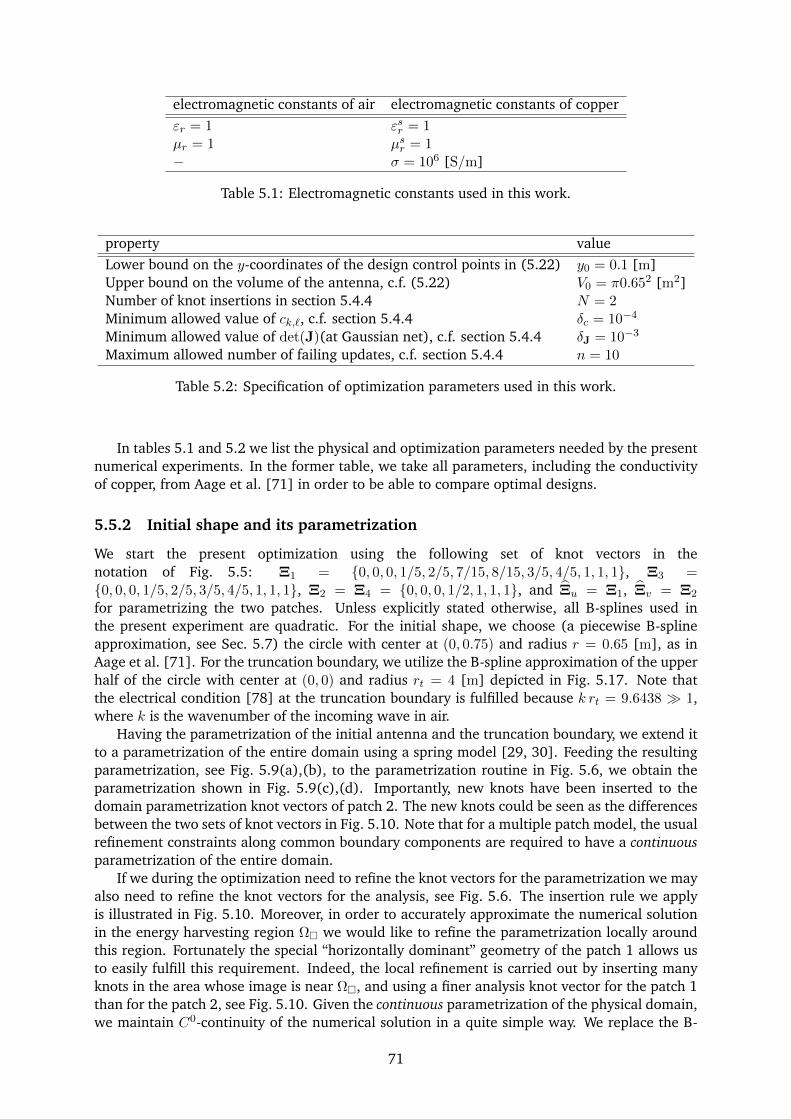
electromagnetic constants of air electromagnetic constants of copperεr = 1 εsr = 1µr = 1 µsr = 1− σ = 106 [S/m]
Table 5.1: Electromagnetic constants used in this work.
property valueLower bound on the y-coordinates of the design control points in (5.22) y0 = 0.1 [m]Upper bound on the volume of the antenna, c.f. (5.22) V0 = π0.652 [m2]Number of knot insertions in section 5.4.4 N = 2Minimum allowed value of ck,`, c.f. section 5.4.4 δc = 10−4
Minimum allowed value of det(J)(at Gaussian net), c.f. section 5.4.4 δJ = 10−3
Maximum allowed number of failing updates, c.f. section 5.4.4 n = 10
Table 5.2: Specification of optimization parameters used in this work.
In tables 5.1 and 5.2 we list the physical and optimization parameters needed by the presentnumerical experiments. In the former table, we take all parameters, including the conductivityof copper, from Aage et al. [71] in order to be able to compare optimal designs.
5.5.2 Initial shape and its parametrization
We start the present optimization using the following set of knot vectors in thenotation of Fig. 5.5: Ξ1 = 0, 0, 0, 1/5, 2/5, 7/15, 8/15, 3/5, 4/5, 1, 1, 1, Ξ3 =0, 0, 0, 1/5, 2/5, 3/5, 4/5, 1, 1, 1, Ξ2 = Ξ4 = 0, 0, 0, 1/2, 1, 1, 1, and Ξu = Ξ1, Ξv = Ξ2
for parametrizing the two patches. Unless explicitly stated otherwise, all B-splines used inthe present experiment are quadratic. For the initial shape, we choose (a piecewise B-splineapproximation, see Sec. 5.7) the circle with center at (0, 0.75) and radius r = 0.65 [m], as inAage et al. [71]. For the truncation boundary, we utilize the B-spline approximation of the upperhalf of the circle with center at (0, 0) and radius rt = 4 [m] depicted in Fig. 5.17. Note thatthe electrical condition [78] at the truncation boundary is fulfilled because k rt = 9.6438 1,where k is the wavenumber of the incoming wave in air.
Having the parametrization of the initial antenna and the truncation boundary, we extend itto a parametrization of the entire domain using a spring model [29, 30]. Feeding the resultingparametrization, see Fig. 5.9(a),(b), to the parametrization routine in Fig. 5.6, we obtain theparametrization shown in Fig. 5.9(c),(d). Importantly, new knots have been inserted to thedomain parametrization knot vectors of patch 2. The new knots could be seen as the differencesbetween the two sets of knot vectors in Fig. 5.10. Note that for a multiple patch model, the usualrefinement constraints along common boundary components are required to have a continuousparametrization of the entire domain.
If we during the optimization need to refine the knot vectors for the parametrization we mayalso need to refine the knot vectors for the analysis, see Fig. 5.6. The insertion rule we applyis illustrated in Fig. 5.10. Moreover, in order to accurately approximate the numerical solutionin the energy harvesting region Ω we would like to refine the parametrization locally aroundthis region. Fortunately the special “horizontally dominant” geometry of the patch 1 allows usto easily fulfill this requirement. Indeed, the local refinement is carried out by inserting manyknots in the area whose image is near Ω, and using a finer analysis knot vector for the patch 1than for the patch 2, see Fig. 5.10. Given the continuous parametrization of the physical domain,we maintain C0-continuity of the numerical solution in a quite simple way. We replace the B-
71
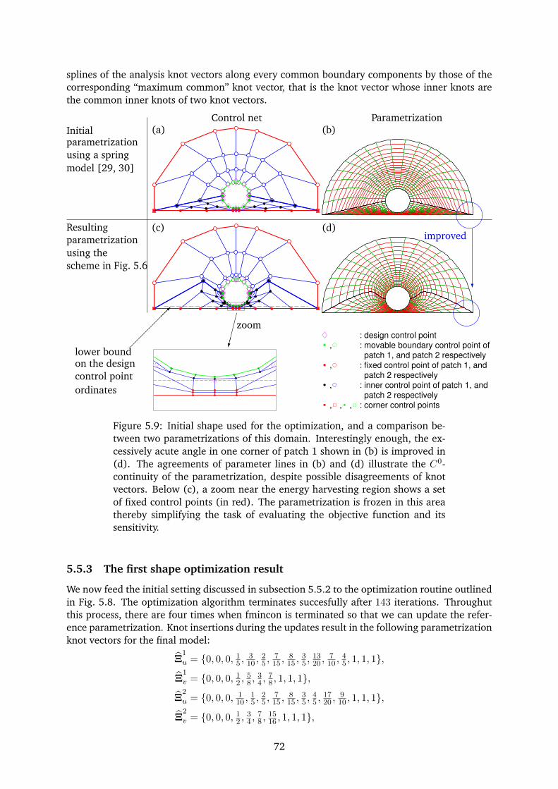
splines of the analysis knot vectors along every common boundary components by those of thecorresponding “maximum common” knot vector, that is the knot vector whose inner knots arethe common inner knots of two knot vectors.
: design control point
, : movable boundary control point of
patch 1, and patch 2 respectively
, : fixed control point of patch 1, and
patch 2 respectively
, : inner control point of patch 1, and
patch 2 respectively
, , , : corner control points
Control net Parametrization
Resultingparametrizationusing thescheme in Fig. 5.6
Initialparametrizationusing a springmodel [29, 30]
zoom
(a) (b)
(c) (d)
?
improved
lower boundon the designcontrol pointordinates
Figure 5.9: Initial shape used for the optimization, and a comparison be-tween two parametrizations of this domain. Interestingly enough, the ex-cessively acute angle in one corner of patch 1 shown in (b) is improved in(d). The agreements of parameter lines in (b) and (d) illustrate the C0-continuity of the parametrization, despite possible disagreements of knotvectors. Below (c), a zoom near the energy harvesting region shows a setof fixed control points (in red). The parametrization is frozen in this areathereby simplifying the task of evaluating the objective function and itssensitivity.
5.5.3 The first shape optimization result
We now feed the initial setting discussed in subsection 5.5.2 to the optimization routine outlinedin Fig. 5.8. The optimization algorithm terminates succesfully after 143 iterations. Throughutthis process, there are four times when fmincon is terminated so that we can update the refer-ence parametrization. Knot insertions during the updates result in the following parametrizationknot vectors for the final model:
Ξ1
u = 0, 0, 0, 15 ,
310 ,
25 ,
715 ,
815 ,
35 ,
1320 ,
710 ,
45 , 1, 1, 1,
Ξ1
v = 0, 0, 0, 12 ,
58 ,
34 ,
78 , 1, 1, 1,
Ξ2
u = 0, 0, 0, 110 ,
15 ,
25 ,
715 ,
815 ,
35 ,
45 ,
1720 ,
910 , 1, 1, 1,
Ξ2
v = 0, 0, 0, 12 ,
34 ,
78 ,
1516 , 1, 1, 1,
72
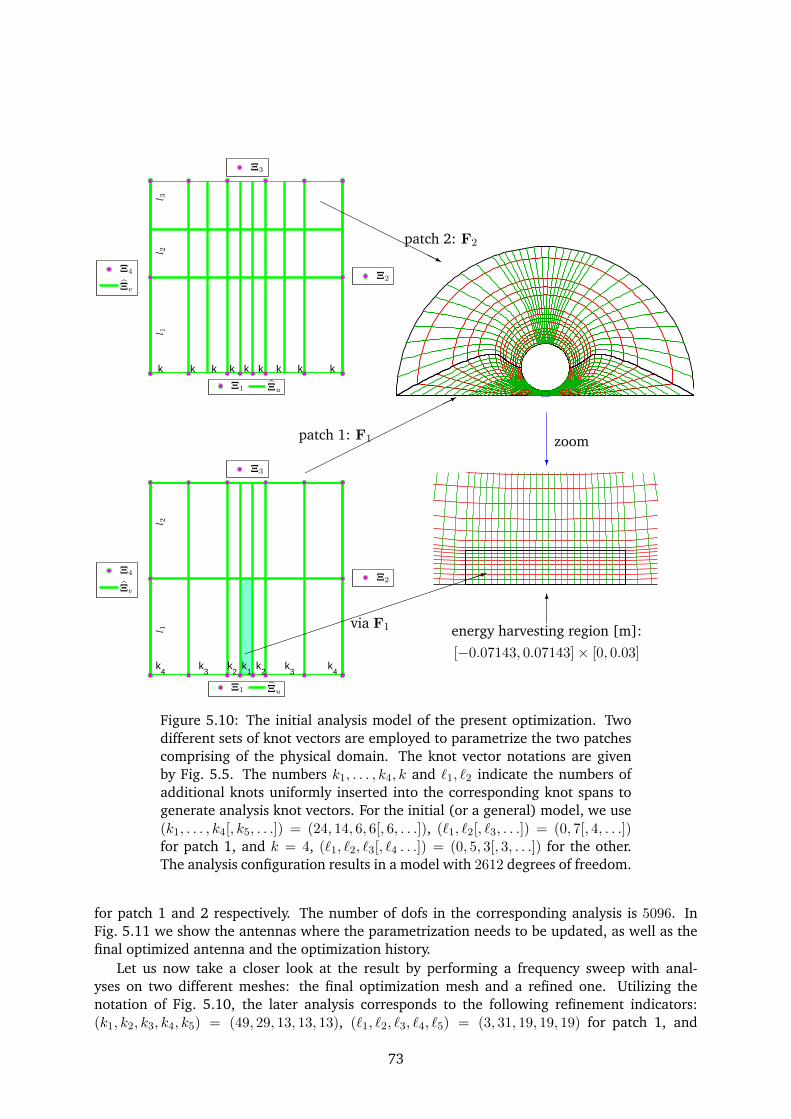
Ξ1 Ξu
Ξ3
Ξ2
k k k k k k k k k
l 1l 2
l 3
Ξ4
Ξv
Ξ1 Ξu
Ξ3
Ξ2
k4
k3
k2
k1
k2
k3
k4
l 1l 2
Ξ4
Ξv
patch 1: F1
*
patch 2: F2
HHHH
HHHHHHj
zoom?
1
via F1
6
energy harvesting region [m]:[−0.07143, 0.07143]× [0, 0.03]
Figure 5.10: The initial analysis model of the present optimization. Twodifferent sets of knot vectors are employed to parametrize the two patchescomprising of the physical domain. The knot vector notations are givenby Fig. 5.5. The numbers k1, . . . , k4, k and `1, `2 indicate the numbers ofadditional knots uniformly inserted into the corresponding knot spans togenerate analysis knot vectors. For the initial (or a general) model, we use(k1, . . . , k4[, k5, . . .]) = (24, 14, 6, 6[, 6, . . .]), (`1, `2[, `3, . . .]) = (0, 7[, 4, . . .])for patch 1, and k = 4, (`1, `2, `3[, `4 . . .]) = (0, 5, 3[, 3, . . .]) for the other.The analysis configuration results in a model with 2612 degrees of freedom.
for patch 1 and 2 respectively. The number of dofs in the corresponding analysis is 5096. InFig. 5.11 we show the antennas where the parametrization needs to be updated, as well as thefinal optimized antenna and the optimization history.
Let us now take a closer look at the result by performing a frequency sweep with anal-yses on two different meshes: the final optimization mesh and a refined one. Utilizing thenotation of Fig. 5.10, the later analysis corresponds to the following refinement indicators:(k1, k2, k3, k4, k5) = (49, 29, 13, 13, 13), (`1, `2, `3, `4, `5) = (3, 31, 19, 19, 19) for patch 1, and
73
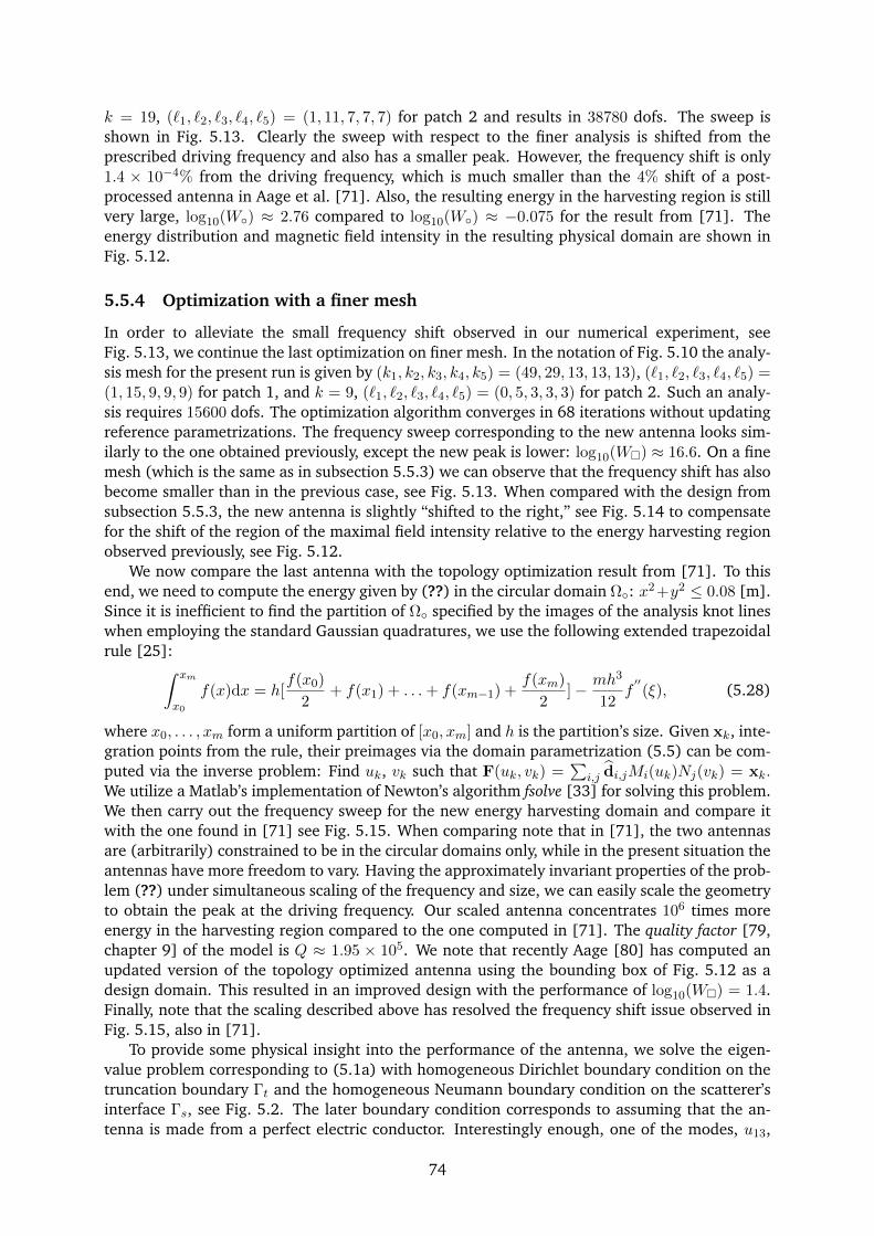
k = 19, (`1, `2, `3, `4, `5) = (1, 11, 7, 7, 7) for patch 2 and results in 38780 dofs. The sweep isshown in Fig. 5.13. Clearly the sweep with respect to the finer analysis is shifted from theprescribed driving frequency and also has a smaller peak. However, the frequency shift is only1.4 × 10−4% from the driving frequency, which is much smaller than the 4% shift of a post-processed antenna in Aage et al. [71]. Also, the resulting energy in the harvesting region is stillvery large, log10(W) ≈ 2.76 compared to log10(W) ≈ −0.075 for the result from [71]. Theenergy distribution and magnetic field intensity in the resulting physical domain are shown inFig. 5.12.
5.5.4 Optimization with a finer mesh
In order to alleviate the small frequency shift observed in our numerical experiment, seeFig. 5.13, we continue the last optimization on finer mesh. In the notation of Fig. 5.10 the analy-sis mesh for the present run is given by (k1, k2, k3, k4, k5) = (49, 29, 13, 13, 13), (`1, `2, `3, `4, `5) =(1, 15, 9, 9, 9) for patch 1, and k = 9, (`1, `2, `3, `4, `5) = (0, 5, 3, 3, 3) for patch 2. Such an analy-sis requires 15600 dofs. The optimization algorithm converges in 68 iterations without updatingreference parametrizations. The frequency sweep corresponding to the new antenna looks sim-ilarly to the one obtained previously, except the new peak is lower: log10(W) ≈ 16.6. On a finemesh (which is the same as in subsection 5.5.3) we can observe that the frequency shift has alsobecome smaller than in the previous case, see Fig. 5.13. When compared with the design fromsubsection 5.5.3, the new antenna is slightly “shifted to the right,” see Fig. 5.14 to compensatefor the shift of the region of the maximal field intensity relative to the energy harvesting regionobserved previously, see Fig. 5.12.
We now compare the last antenna with the topology optimization result from [71]. To thisend, we need to compute the energy given by (??) in the circular domain Ω: x2+y2 ≤ 0.08 [m].Since it is inefficient to find the partition of Ω specified by the images of the analysis knot lineswhen employing the standard Gaussian quadratures, we use the following extended trapezoidalrule [25]:
∫ xm
x0
f(x)dx = h[f(x0)
2+ f(x1) + . . .+ f(xm−1) +
f(xm)
2]− mh3
12f′′(ξ), (5.28)
where x0, . . . , xm form a uniform partition of [x0, xm] and h is the partition’s size. Given xk, inte-gration points from the rule, their preimages via the domain parametrization (5.5) can be com-puted via the inverse problem: Find uk, vk such that F(uk, vk) =
∑i,j di,jMi(uk)Nj(vk) = xk.
We utilize a Matlab’s implementation of Newton’s algorithm fsolve [33] for solving this problem.We then carry out the frequency sweep for the new energy harvesting domain and compare itwith the one found in [71] see Fig. 5.15. When comparing note that in [71], the two antennasare (arbitrarily) constrained to be in the circular domains only, while in the present situation theantennas have more freedom to vary. Having the approximately invariant properties of the prob-lem (??) under simultaneous scaling of the frequency and size, we can easily scale the geometryto obtain the peak at the driving frequency. Our scaled antenna concentrates 106 times moreenergy in the harvesting region compared to the one computed in [71]. The quality factor [79,chapter 9] of the model is Q ≈ 1.95 × 10⁵. We note that recently Aage [80] has computed anupdated version of the topology optimized antenna using the bounding box of Fig. 5.12 as adesign domain. This resulted in an improved design with the performance of log10(W) = 1.4.Finally, note that the scaling described above has resolved the frequency shift issue observed inFig. 5.15, also in [71].
To provide some physical insight into the performance of the antenna, we solve the eigen-value problem corresponding to (5.1a) with homogeneous Dirichlet boundary condition on thetruncation boundary Γt and the homogeneous Neumann boundary condition on the scatterer’sinterface Γs, see Fig. 5.2. The later boundary condition corresponds to assuming that the an-tenna is made from a perfect electric conductor. Interestingly enough, one of the modes, u13,
74
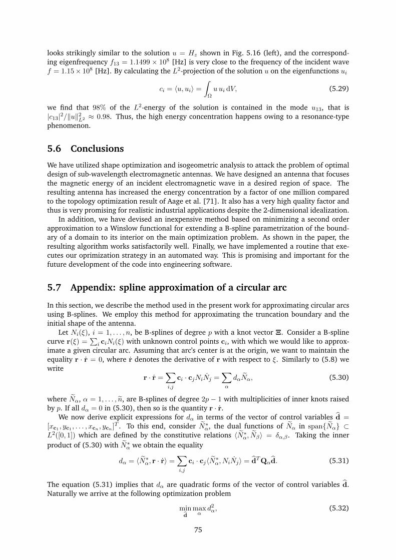
looks strikingly similar to the solution u = Hz shown in Fig. 5.16 (left), and the correspond-ing eigenfrequency f13 = 1.1499 × 10⁸ [Hz] is very close to the frequency of the incident wavef = 1.15× 10⁸ [Hz]. By calculating the L2-projection of the solution u on the eigenfunctions ui
ci = 〈u, ui〉 =
∫
Ωuui dV, (5.29)
we find that 98% of the L2-energy of the solution is contained in the mode u13, that is|c13|2/‖u‖2L2 ≈ 0.98. Thus, the high energy concentration happens owing to a resonance-typephenomenon.
5.6 Conclusions
We have utilized shape optimization and isogeometric analysis to attack the problem of optimaldesign of sub-wavelength electromagnetic antennas. We have designed an antenna that focusesthe magnetic energy of an incident electromagnetic wave in a desired region of space. Theresulting antenna has increased the energy concentration by a factor of one million comparedto the topology optimization result of Aage et al. [71]. It also has a very high quality factor andthus is very promising for realistic industrial applications despite the 2-dimensional idealization.
In addition, we have devised an inexpensive method based on minimizing a second orderapproximation to a Winslow functional for extending a B-spline parametrization of the bound-ary of a domain to its interior on the main optimization problem. As shown in the paper, theresulting algorithm works satisfactorily well. Finally, we have implemented a routine that exe-cutes our oprimization strategy in an automated way. This is promising and important for thefuture development of the code into engineering software.
5.7 Appendix: spline approximation of a circular arc
In this section, we describe the method used in the present work for approximating circular arcsusing B-splines. We employ this method for approximating the truncation boundary and theinitial shape of the antenna.
Let Ni(ξ), i = 1, . . . , n, be B-splines of degree p with a knot vector Ξ. Consider a B-splinecurve r(ξ) =
∑i ciNi(ξ) with unknown control points ci, with which we would like to approx-
imate a given circular arc. Assuming that arc’s center is at the origin, we want to maintain theequality r · r = 0, where r denotes the derivative of r with respect to ξ. Similarly to (5.8) wewrite
r · r =∑
i,j
ci · cjNiNj =∑
α
dαNα, (5.30)
where Nα, α = 1, . . . , n, are B-splines of degree 2p − 1 with multiplicities of inner knots raisedby p. If all dα = 0 in (5.30), then so is the quantity r · r.
We now derive explicit expressions for dα in terms of the vector of control variables d =[xc1 , yc1 , . . . , xcn , ycn ]T . To this end, consider N∗α, the dual functions of Nα in spanNα ⊂L2([0, 1]) which are defined by the constitutive relations 〈N∗α, Nβ〉 = δα,β. Taking the innerproduct of (5.30) with N∗α we obtain the equality
dα = 〈N∗α, r · r〉 =∑
i,j
ci · cj〈N∗α, NiNj〉 = dTQαd. (5.31)
The equation (5.31) implies that dα are quadratic forms of the vector of control variables d.Naturally we arrive at the following optimization problem
mind
maxα
d2α, (5.32)
75

which can be numerically solved to approximate stationarity using the same approach as theoptimization problem (5.9). Utilizing (5.32), we obtain a good approximation for the circulartruncation boundary, see Fig. 5.17.
76
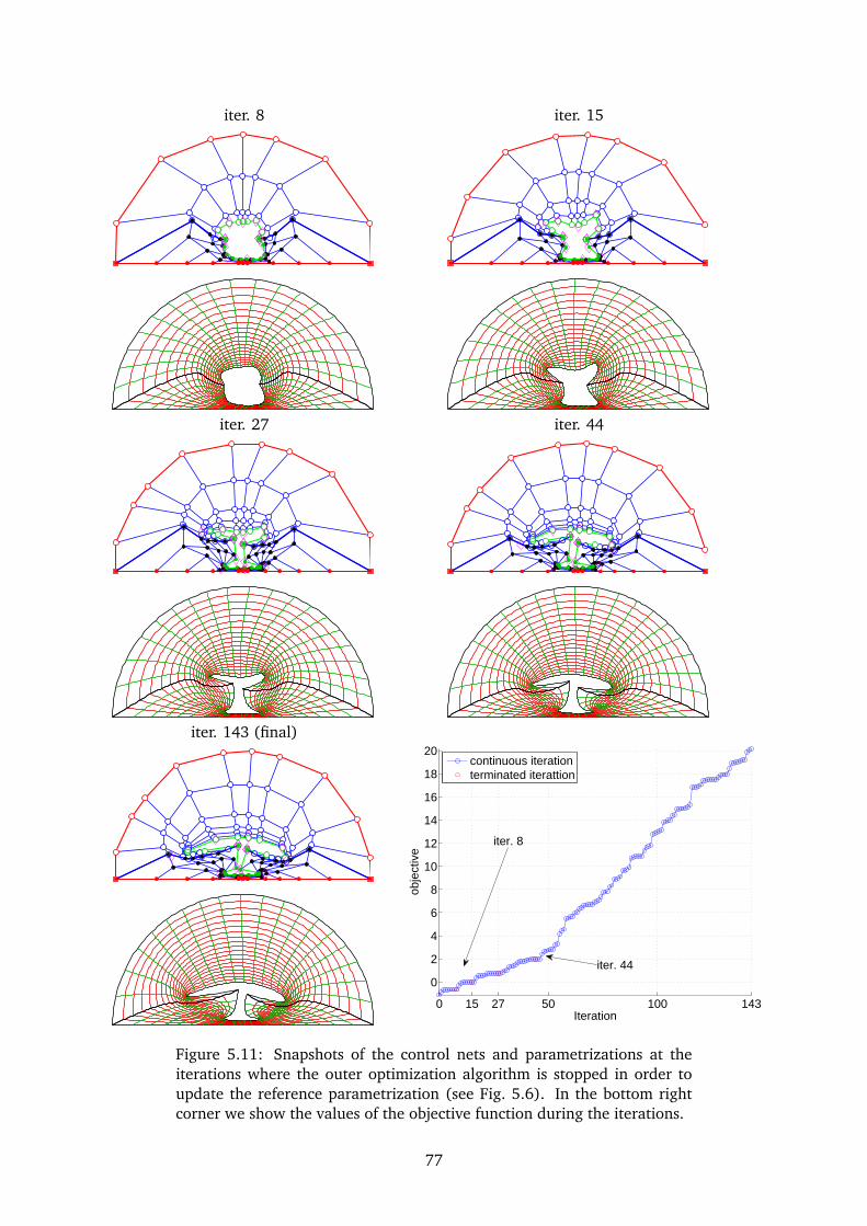
iter. 8 iter. 15
iter. 27 iter. 44
iter. 143 (final)
0 15 27 50 100 143
0
2
4
6
8
10
12
14
16
18
20
Iteration
obje
ctiv
e
continuous iterationterminated iterattion
iter. 8
iter. 44
Figure 5.11: Snapshots of the control nets and parametrizations at theiterations where the outer optimization algorithm is stopped in order toupdate the reference parametrization (see Fig. 5.6). In the bottom rightcorner we show the values of the objective function during the iterations.
77
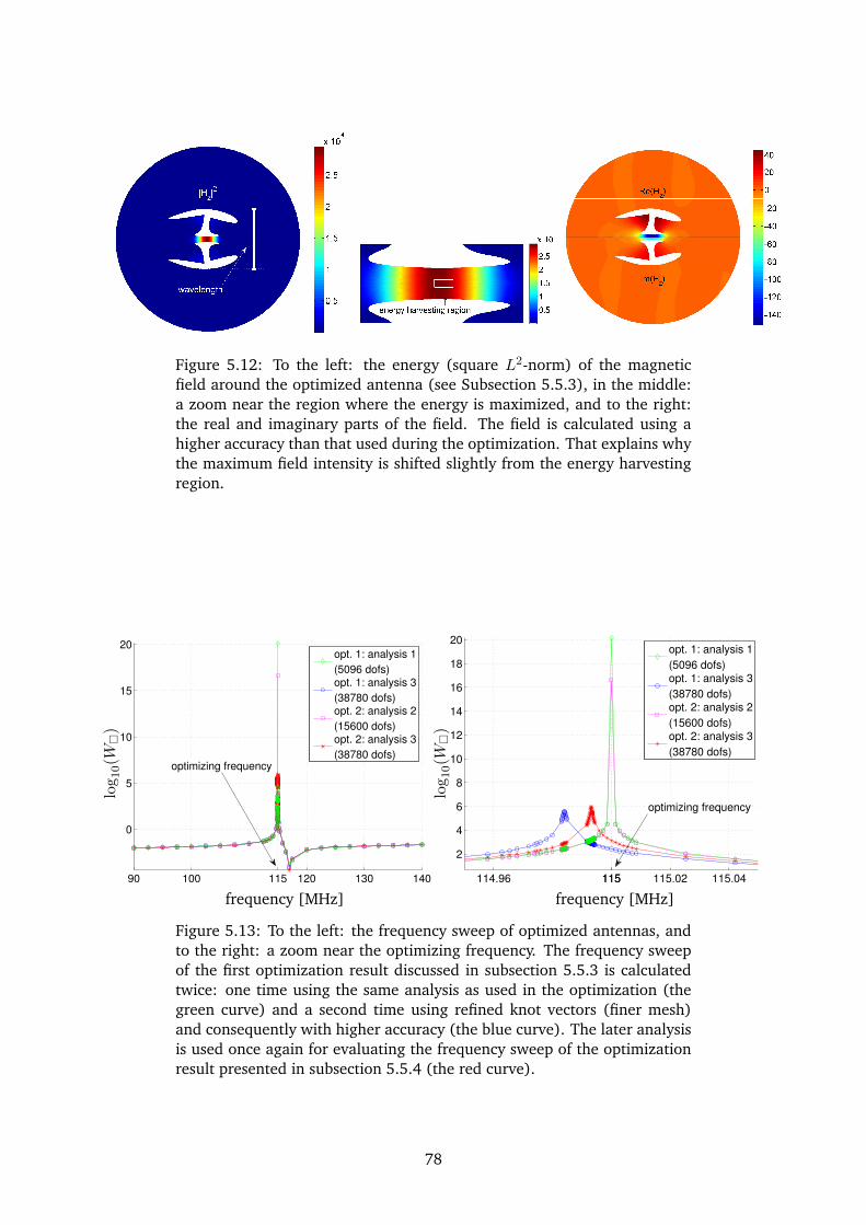
Figure 5.12: To the left: the energy (square L2-norm) of the magneticfield around the optimized antenna (see Subsection 5.5.3), in the middle:a zoom near the region where the energy is maximized, and to the right:the real and imaginary parts of the field. The field is calculated using ahigher accuracy than that used during the optimization. That explains whythe maximum field intensity is shifted slightly from the energy harvestingregion.
90 100 115 120 130 140
0
5
10
15
20
opt. 1: analysis 1
(5096 dofs)
opt. 1: analysis 3
(38780 dofs)opt. 2: analysis 2
(15600 dofs)
opt. 2: analysis 3
(38780 dofs)optimizing frequency
114.96 115115 115.02 115.04
2
4
6
8
10
12
14
16
18
20
opt. 1: analysis 1
(5096 dofs)
opt. 1: analysis 3
(38780 dofs)opt. 2: analysis 2
(15600 dofs)
opt. 2: analysis 3
(38780 dofs)
optimizing frequency
frequency [MHz]
log
10(W
)
frequency [MHz]
log
10(W
)
Figure 5.13: To the left: the frequency sweep of optimized antennas, andto the right: a zoom near the optimizing frequency. The frequency sweepof the first optimization result discussed in subsection 5.5.3 is calculatedtwice: one time using the same analysis as used in the optimization (thegreen curve) and a second time using refined knot vectors (finer mesh)and consequently with higher accuracy (the blue curve). The later analysisis used once again for evaluating the frequency sweep of the optimizationresult presented in subsection 5.5.4 (the red curve).
78
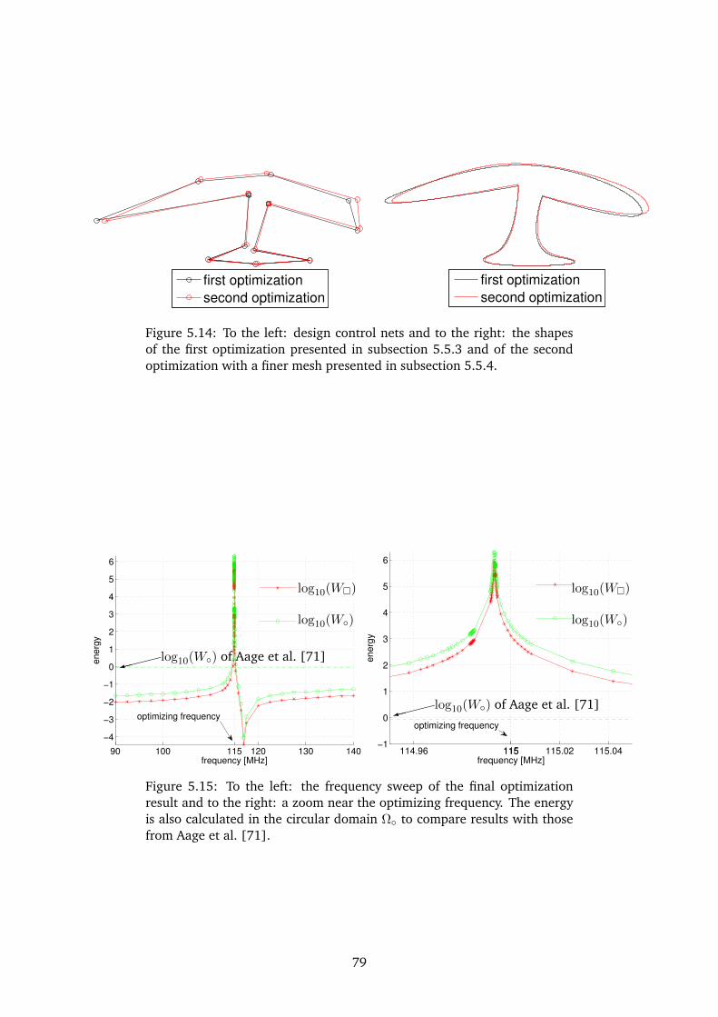
first optimization
second optimization
first optimization
second optimization
Figure 5.14: To the left: design control nets and to the right: the shapesof the first optimization presented in subsection 5.5.3 and of the secondoptimization with a finer mesh presented in subsection 5.5.4.
90 100 115 120 130 140
−4
−3
−2
−1
0
1
2
3
4
5
6
frequency [MHz]
en
erg
y
optimizing frequency
114.96 115115 115.02 115.04−1
0
1
2
3
4
5
6
frequency [MHz]
en
erg
y
optimizing frequency
log10(W)
log10(W)
log10(W)
log10(W)
log10(W) of Aage et al. [71]9
log10(W) of Aage et al. [71]9
Figure 5.15: To the left: the frequency sweep of the final optimizationresult and to the right: a zoom near the optimizing frequency. The energyis also calculated in the circular domain Ω to compare results with thosefrom Aage et al. [71].
79
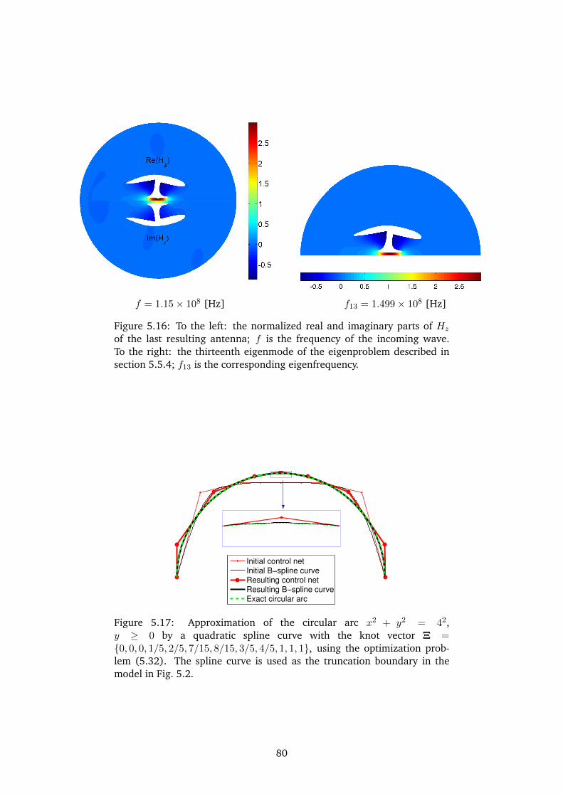
f = 1.15× 10⁸ [Hz] f13 = 1.499× 10⁸ [Hz]
Figure 5.16: To the left: the normalized real and imaginary parts of Hz
of the last resulting antenna; f is the frequency of the incoming wave.To the right: the thirteenth eigenmode of the eigenproblem described insection 5.5.4; f13 is the corresponding eigenfrequency.
Initial control net
Initial B−spline curve
Resulting control net
Resulting B−spline curve
Exact circular arc
?
Figure 5.17: Approximation of the circular arc x2 + y2 = 42,y ≥ 0 by a quadratic spline curve with the knot vector Ξ =0, 0, 0, 1/5, 2/5, 7/15, 8/15, 3/5, 4/5, 1, 1, 1, using the optimization prob-lem (5.32). The spline curve is used as the truncation boundary in themodel in Fig. 5.2.
80
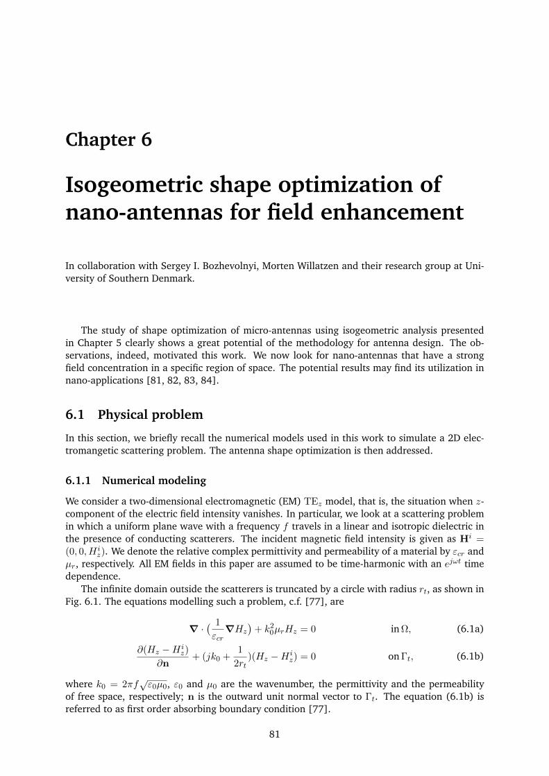
Chapter 6
Isogeometric shape optimization ofnano-antennas for field enhancement
In collaboration with Sergey I. Bozhevolnyi, Morten Willatzen and their research group at Uni-versity of Southern Denmark.
The study of shape optimization of micro-antennas using isogeometric analysis presentedin Chapter 5 clearly shows a great potential of the methodology for antenna design. The ob-servations, indeed, motivated this work. We now look for nano-antennas that have a strongfield concentration in a specific region of space. The potential results may find its utilization innano-applications [81, 82, 83, 84].
6.1 Physical problem
In this section, we briefly recall the numerical models used in this work to simulate a 2D elec-tromangetic scattering problem. The antenna shape optimization is then addressed.
6.1.1 Numerical modeling
We consider a two-dimensional electromagnetic (EM) TEz model, that is, the situation when z-component of the electric field intensity vanishes. In particular, we look at a scattering problemin which a uniform plane wave with a frequency f travels in a linear and isotropic dielectric inthe presence of conducting scatterers. The incident magnetic field intensity is given as Hi =(0, 0, H i
z). We denote the relative complex permittivity and permeability of a material by εcr andµr, respectively. All EM fields in this paper are assumed to be time-harmonic with an ejωt timedependence.
The infinite domain outside the scatterers is truncated by a circle with radius rt, as shown inFig. 6.1. The equations modelling such a problem, c.f. [77], are
∇ ·( 1
εcr∇Hz
)+ k2
0µrHz = 0 in Ω, (6.1a)
∂(Hz −H iz)
∂n+ (jk0 +
1
2rt)(Hz −H i
z) = 0 on Γt, (6.1b)
where k0 = 2πf√ε0µ0, ε0 and µ0 are the wavenumber, the permittivity and the permeability
of free space, respectively; n is the outward unit normal vector to Γt. The equation (6.1b) isreferred to as first order absorbing boundary condition [77].
81
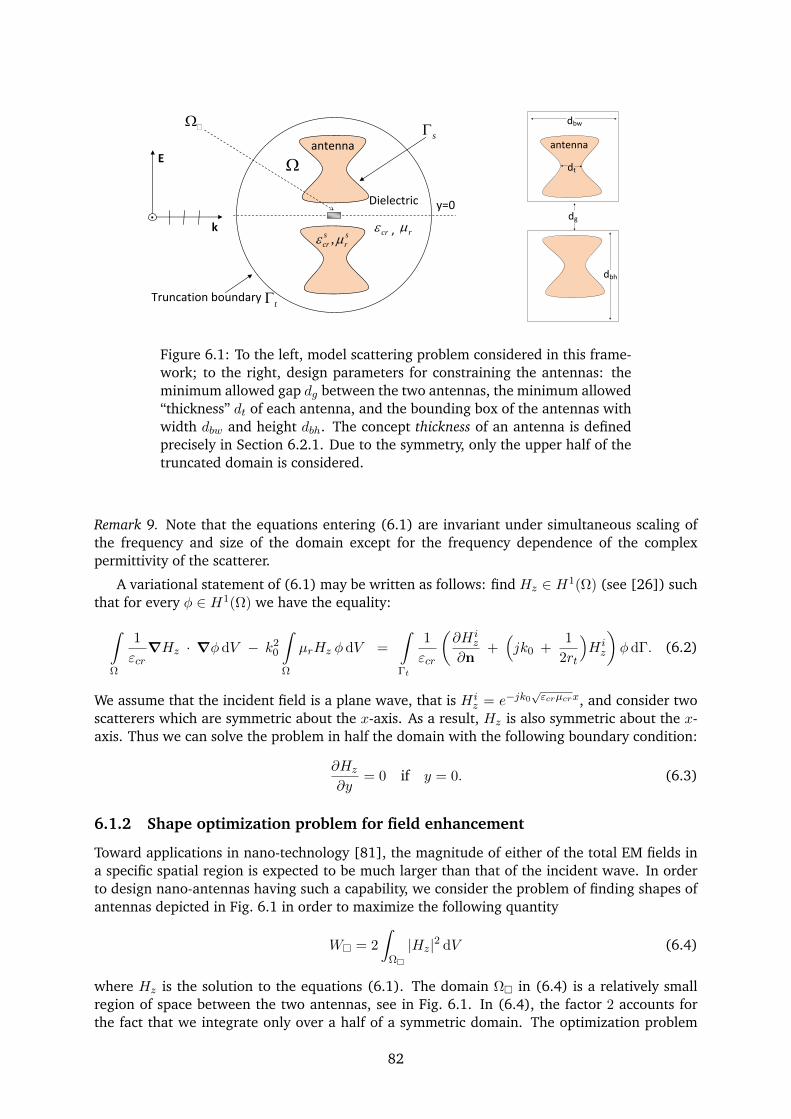
antenna
k H
E
.
Truncation boundary
Dielectric
cr , r ,s s
cr r
s
t
y=0
dg
dbw
dt
dbh
antenna
Figure 6.1: To the left, model scattering problem considered in this frame-work; to the right, design parameters for constraining the antennas: theminimum allowed gap dg between the two antennas, the minimum allowed“thickness” dt of each antenna, and the bounding box of the antennas withwidth dbw and height dbh. The concept thickness of an antenna is definedprecisely in Section 6.2.1. Due to the symmetry, only the upper half of thetruncated domain is considered.
Remark 9. Note that the equations entering (6.1) are invariant under simultaneous scaling ofthe frequency and size of the domain except for the frequency dependence of the complexpermittivity of the scatterer.
A variational statement of (6.1) may be written as follows: find Hz ∈ H1(Ω) (see [26]) suchthat for every φ ∈ H1(Ω) we have the equality:
∫
Ω
1
εcr∇Hz · ∇φ dV − k2
0
∫
Ω
µrHz φ dV =
∫
Γt
1
εcr
(∂H i
z
∂n+(jk0 +
1
2rt
)H iz
)φ dΓ. (6.2)
We assume that the incident field is a plane wave, that is H iz = e−jk0
√εcrµcrx, and consider two
scatterers which are symmetric about the x-axis. As a result, Hz is also symmetric about the x-axis. Thus we can solve the problem in half the domain with the following boundary condition:
∂Hz
∂y= 0 if y = 0. (6.3)
6.1.2 Shape optimization problem for field enhancement
Toward applications in nano-technology [81], the magnitude of either of the total EM fields ina specific spatial region is expected to be much larger than that of the incident wave. In orderto design nano-antennas having such a capability, we consider the problem of finding shapes ofantennas depicted in Fig. 6.1 in order to maximize the following quantity
W = 2
∫
Ω
|Hz|2 dV (6.4)
where Hz is the solution to the equations (6.1). The domain Ω in (6.4) is a relatively smallregion of space between the two antennas, see in Fig. 6.1. In (6.4), the factor 2 accounts forthe fact that we integrate only over a half of a symmetric domain. The optimization problem
82
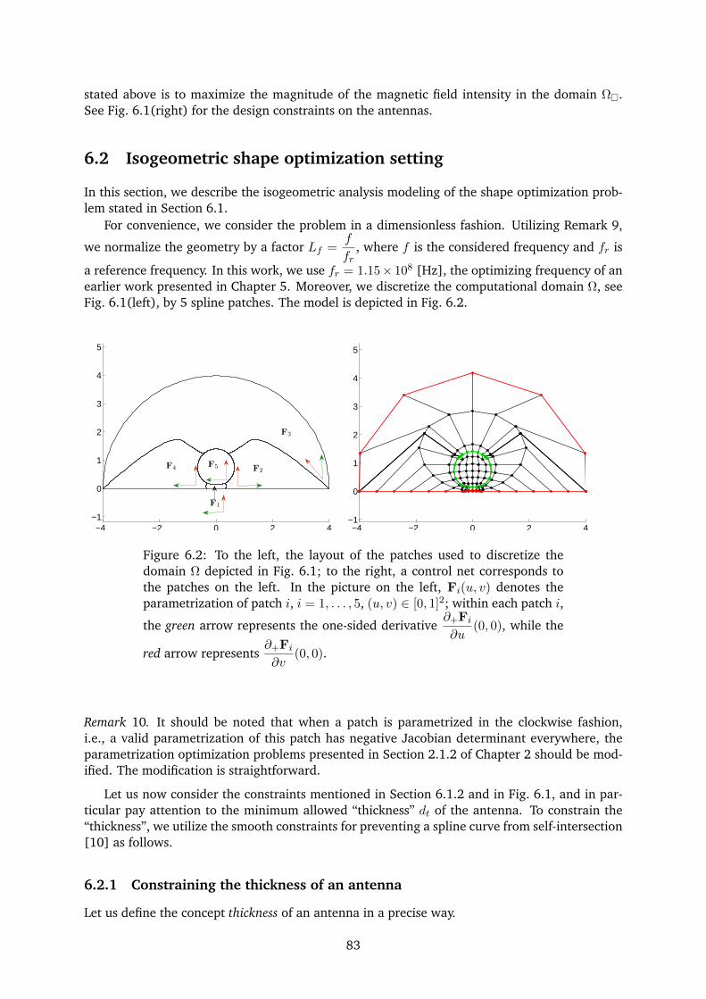
stated above is to maximize the magnitude of the magnetic field intensity in the domain Ω.See Fig. 6.1(right) for the design constraints on the antennas.
6.2 Isogeometric shape optimization setting
In this section, we describe the isogeometric analysis modeling of the shape optimization prob-lem stated in Section 6.1.
For convenience, we consider the problem in a dimensionless fashion. Utilizing Remark 9,
we normalize the geometry by a factor Lf =f
fr, where f is the considered frequency and fr is
a reference frequency. In this work, we use fr = 1.15× 10⁸ [Hz], the optimizing frequency of anearlier work presented in Chapter 5. Moreover, we discretize the computational domain Ω, seeFig. 6.1(left), by 5 spline patches. The model is depicted in Fig. 6.2.
−4 −2 0 2 4−1
0
1
2
3
4
5
F2F4
F1
F3
F5
−4 −2 0 2 4−1
0
1
2
3
4
5
Figure 6.2: To the left, the layout of the patches used to discretize thedomain Ω depicted in Fig. 6.1; to the right, a control net corresponds tothe patches on the left. In the picture on the left, Fi(u, v) denotes theparametrization of patch i, i = 1, . . . , 5, (u, v) ∈ [0, 1]2; within each patch i,
the green arrow represents the one-sided derivative∂+Fi
∂u(0, 0), while the
red arrow represents∂+Fi
∂v(0, 0).
Remark 10. It should be noted that when a patch is parametrized in the clockwise fashion,i.e., a valid parametrization of this patch has negative Jacobian determinant everywhere, theparametrization optimization problems presented in Section 2.1.2 of Chapter 2 should be mod-ified. The modification is straightforward.
Let us now consider the constraints mentioned in Section 6.1.2 and in Fig. 6.1, and in par-ticular pay attention to the minimum allowed “thickness” dt of the antenna. To constrain the“thickness”, we utilize the smooth constraints for preventing a spline curve from self-intersection[10] as follows.
6.2.1 Constraining the thickness of an antenna
Let us define the concept thickness of an antenna in a precise way.
83
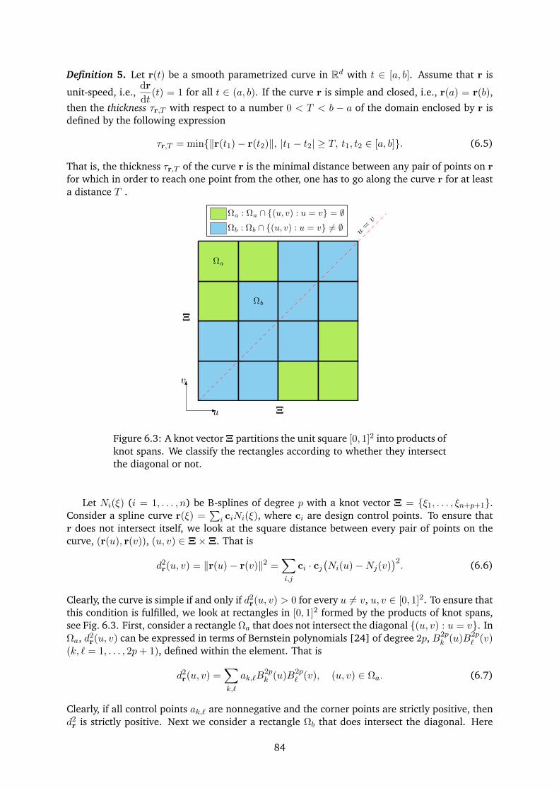
Definition 5. Let r(t) be a smooth parametrized curve in Rd with t ∈ [a, b]. Assume that r is
unit-speed, i.e.,dr
dt(t) = 1 for all t ∈ (a, b). If the curve r is simple and closed, i.e., r(a) = r(b),
then the thickness τr,T with respect to a number 0 < T < b − a of the domain enclosed by r isdefined by the following expression
τr,T = min‖r(t1)− r(t2)‖, |t1 − t2| ≥ T, t1, t2 ∈ [a, b]. (6.5)
That is, the thickness τr,T of the curve r is the minimal distance between any pair of points on rfor which in order to reach one point from the other, one has to go along the curve r for at leasta distance T .
u=v
Ωa
Ωb
Ωa : Ωa ∩ (u, v) : u = v = ∅Ωb : Ωb ∩ (u, v) : u = v 6= ∅
-
6
u
v
Ξ
Ξ
Figure 6.3: A knot vector Ξ partitions the unit square [0, 1]2 into products ofknot spans. We classify the rectangles according to whether they intersectthe diagonal or not.
Let Ni(ξ) (i = 1, . . . , n) be B-splines of degree p with a knot vector Ξ = ξ1, . . . , ξn+p+1.Consider a spline curve r(ξ) =
∑i ciNi(ξ), where ci are design control points. To ensure that
r does not intersect itself, we look at the square distance between every pair of points on thecurve, (r(u), r(v)), (u, v) ∈ Ξ×Ξ. That is
d2r(u, v) = ‖r(u)− r(v)‖2 =
∑
i,j
ci · cj(Ni(u)−Nj(v)
)2. (6.6)
Clearly, the curve is simple if and only if d2r(u, v) > 0 for every u 6= v, u, v ∈ [0, 1]2. To ensure that
this condition is fulfilled, we look at rectangles in [0, 1]2 formed by the products of knot spans,see Fig. 6.3. First, consider a rectangle Ωa that does not intersect the diagonal (u, v) : u = v. InΩa, d2
r(u, v) can be expressed in terms of Bernstein polynomials [24] of degree 2p, B2pk (u)B2p
` (v)(k, ` = 1, . . . , 2p+ 1), defined within the element. That is
d2r(u, v) =
∑
k,`
ak,`B2pk (u)B2p
` (v), (u, v) ∈ Ωa. (6.7)
Clearly, if all control points ak,` are nonnegative and the corner points are strictly positive, thend2r is strictly positive. Next we consider a rectangle Ωb that does intersect the diagonal. Here
84
(u− v)2 is a factor of d2r and we can write
d2r(u, v) = (u− v)2
∑
α,β
bα,βB2p−2α (u)B2p−2
β (v) (u, v) ∈ Ωb (6.8)
In (6.8), B2p−2α (u)B2p−2
β (v) (α, β = 1, . . . , 2p − 1) are Bernstein polynomials of degree 2p − 2defined within Ωb. Once again, if all control points ak,` are non negative and the corner pointsare strictly positive, then dr is strictly positive. So we arrive at the sufficient conditions: Thecurve r is a simple curve if the following conditions are satisfied
(i) ak,` ≥ 0 for all k, ` = 1, . . . , 2p+ 1,
(ii) bα,β ≥ 0 for all α, β = 1, . . . , 2p− 1,
(iii) d2r(ξi, ξj) ≥ δ, i, j = 1, . . . , n, for some positive δ.
To further constrain the minimum allowed thickness dt of the antenna, inspired by Definition6.5, we replace the constraints (i) above with the following
(i-1) ak1,`1 ≥ 0 for all k1, `1 = 1, . . . , 2p + 1, if the corresponding supporting domain Ωa =[ξr, ξr+1]× [ξs, ξs+1] are with |r − s| < nk,
(i-2) ak2,`2 ≥ d2t for all k2, `2 = 1, . . . , 2p + 1,if the corresponding supporting domain Ωa =
[ξr, ξr+1]× [ξs, ξs+1] are with |r − s| ≥ nk,
where nk ∈ N is the difference in the ordering of the knot intervals [ξr, ξr+1] and [ξs, ξs+1] in allknot intervals with respect to the knot vector Ξ. In this work, we use nk = 3.
Note that utilizing the symmetry in (6.6) about the line u = v, only one half of the condi-tions are needed. Also, similarly to (2.6), the coefficients ak,` in (6.7) and bα,β in (6.8) may beexplicitly represented as quadratic forms of the design control points ci. For the current opti-mization problem, the antenna boundary is composed of two spline curves. Proposition 1 can bestraightforwardly extended to a piecewise spline curve. Finally, knot insertions may be neededin order to obtain tighter conditions for the sufficiency.
6.2.2 Parametrization of a given domain
In an optimization problem using IGA, often the objective function is given by the integral overa given domain in the physical space. To simplify the implementation of IGA when the standardGaussian quadratures [25] are used for numerical integrations, we would like the boundaryof the domain to be the images of knot lines in the parameter space via a parametrization ofthe physical space. This leads to the standard interpolation problem [23] and can be solved asfollows.
Let r(u) = c1N1(u) + . . . + cnNn(u) be a B-spline curve of degree p, where Nk are B-splinewith knot vector Ξ = u1, . . . , uN and ck ∈ Rd, k = 1, . . . , n. For simplicity, assume that allinner knots of Ξ have multiplicity 1. Note that the image of any knot uk via r is a convexcombination of the control points whose corresponding B-splines do not vanish at the knot.Indeed, if we repeat inserting uk into Ξ in p − 1 times, then the resulting control point withrespect to the B-spline defined by the knots
uk−1, uk, . . . , uk︸ ︷︷ ︸p times
, uk+1
must be r(uk). By that way, we can formulate explicitly the weights of the convex combination.For instance if p = 2 we have
r(uk) = (1− αk)ck−2 + αkck−1, k = p+ 1, . . . , n+ 1, (6.9)
85
where αk =uk − uk−1
uk+1 − uk−1. If r(uk), k = p + 1, . . . , n + 1, are given, then (6.9) are a system of
d(n− p+ 1) linear equations of dn unknowns, the coordinates of the control points ck. Thus thecurve r is completely defined if r(uk), k = p+ 1, . . . , n+ 1 are given together with other d(p− 1)linear equations. In this work, the remaining conditions are chosen to be p−1 predefined controlpoints c2, . . . , cp.
6.2.3 Discretization
An approximation to the solution Hz to (6.1) is expanded in terms of the basis functions (seeSection 1.2.1) as Hz =
∑k hk (Rp,qk F−1) =
[Rp,q1 F−1, . . . , Rp,qmn F−1
]h, where h contains
all the coordinates of Hz with respect to the selected basis. Substituting this expression into theweak form (6.2) and utilizing the basis functions as the test functions, we arrive at the followingset of linear algebraic equations:
(K + M + T) h = f . (6.10)
Entries of the matrices entering (6.10) are calculated as:
Kk` =
∫∫
[0,1]2
1
εcr
(DRp,qk (u, v) J−1
)TDRp,q` (u, v) J−1 det(J) dudv, (6.11a)
Mk` = −k20
∫∫
[0,1]2
µr Rp,qk (u, v) Rp,q` (u, v) det(J) dudv, (6.11b)
Tk` =(jk0 +
1
2rt
) ∫
F−1(Γt)
1
εcrRp,qk (u, v) Rp,q` (u, v) ds, (6.11c)
f` =
∫
F−1(Γt)
1
εcr
(∂H i
z
∂n+(jk0 +
1
2rt
)H iz
)Rp,q` (u, v) ds, (6.11d)
k, ` = 1, . . . , mn. In the equations (6.11), J is the Jacobian of the parametrization F andDf(u, v) =
[∂f∂u(u, v) ∂f
∂v (u, v)]
is the differential of a real-valued function f : [0, 1]2 → R.
6.2.4 Formulation of the optimization problem and sensitivity analysis
Recall that d is the vector containing components of design control points, see Fig. 6.4. Takingthe constraints discussed above into account and noting that in (6.4), HzF =
[Rp,q1 , . . . , Rp,qmn
]h,
we arrive at the following shape optimization problem:
maximized∈RN
log10(W) = log10
(2
∫∫
F−1(Ω)
∣∣[Rp,q1 , . . . , Rp,qmn]h∣∣2 det(J) dudv
), (6.12a)
such that yd ≥ y0, (6.12b)
ak1,`1 ≥ 0, ak2,`2 ≥ d2t , bα,β ≥ 0, d2
r(ξi, ξj) ≥ δ, (c.f. Section 6.2.1) (6.12c)
(K + M + T) h = f , (6.12d)
where yd are the y-coordinates of the design control points, and y0 is a lower bound.Let us now find first order derivatives of functions involved in (6.12). First, consider the con-
straints (6.12c). As noted in subsection 6.2.1 the quantities ak,`, bα,β, and dr(ξi, ξj) in (i− iii) ofProposition 1 are quadratic forms of the design control point vector d, therefore evaluating theirgradients with respect to d is a straightforward calculation. On the other hand, the objectivefunction in (6.12) depends implicitly on d through the discretized Maxwell’s equations (6.12d).
86
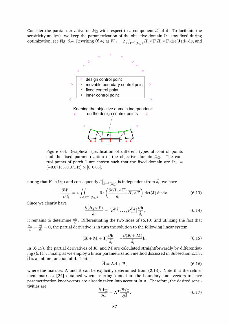
Consider the partial derivative of W with respect to a component di of d. To facilitate thesensitivity analysis, we keep the parametrization of the objective domain Ω stay fixed duringoptimization, see Fig. 6.4. Rewriting (6.4) as W = 2
∫∫F−1(Ω)Hz FHz F det(J) du dv, and
design control pointmovable boundary control pointfixed control pointinner control point
Keeping the objective domain independenton the design control points
Figure 6.4: Graphical specification of different types of control pointsand the fixed parametrization of the objective domain Ω. The con-trol points of patch 1 are chosen such that the fixed domain are Ω =[−0.07143, 0.07143]× [0, 0.03].
noting that F−1(Ω) and consequently J∣∣F−1(Ω)
is independent from di, we have
∂W
∂di= 4
∫∫
F−1(Ω)Re
(∂(Hz F)
diHz F
)det(J) dudv. (6.13)
Since we clearly have∂(Hz F)
di=[Rp,q1 , . . . , Rp,qmn
]∂h
di, (6.14)
it remains to determine ∂hdi
. Differentiating the two sides of (6.10) and utilizing the fact that∂Tdi
= ∂fdi
= 0, the partial derivative is in turn the solution to the following linear system
(K + M + T)∂h
di= −∂(K + M)
dih. (6.15)
In (6.15), the partial derivatives of K, and M are calculated straightforwardly by differentiat-ing (6.11). Finally, as we employ a linear parametrization method discussed in Subsection 2.1.3,d is an affine function of d. That is
d = Ad + B, (6.16)
where the matrices A and B can be explicitly determined from (2.13). Note that the refine-ment matrices [24] obtained when inserting knots into the boundary knot vectors to haveparametrization knot vectors are already taken into account in A. Therefore, the desired sensi-tivities are
∂W
∂d= AT∂W
∂d. (6.17)
87
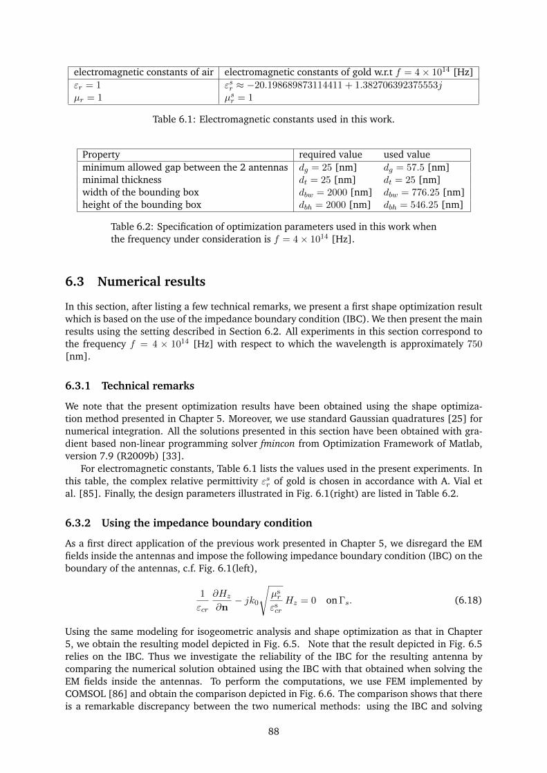
electromagnetic constants of air electromagnetic constants of gold w.r.t f = 4× 10¹⁴ [Hz]εr = 1 εsr ≈ −20.198689873114411 + 1.382706392375553jµr = 1 µsr = 1
Table 6.1: Electromagnetic constants used in this work.
Property required value used valueminimum allowed gap between the 2 antennas dg = 25 [nm] dg = 57.5 [nm]minimal thickness dt = 25 [nm] dt = 25 [nm]width of the bounding box dbw = 2000 [nm] dbw = 776.25 [nm]height of the bounding box dbh = 2000 [nm] dbh = 546.25 [nm]
Table 6.2: Specification of optimization parameters used in this work whenthe frequency under consideration is f = 4× 10¹⁴ [Hz].
6.3 Numerical results
In this section, after listing a few technical remarks, we present a first shape optimization resultwhich is based on the use of the impedance boundary condition (IBC). We then present the mainresults using the setting described in Section 6.2. All experiments in this section correspond tothe frequency f = 4 × 10¹⁴ [Hz] with respect to which the wavelength is approximately 750[nm].
6.3.1 Technical remarks
We note that the present optimization results have been obtained using the shape optimiza-tion method presented in Chapter 5. Moreover, we use standard Gaussian quadratures [25] fornumerical integration. All the solutions presented in this section have been obtained with gra-dient based non-linear programming solver fmincon from Optimization Framework of Matlab,version 7.9 (R2009b) [33].
For electromagnetic constants, Table 6.1 lists the values used in the present experiments. Inthis table, the complex relative permittivity εsr of gold is chosen in accordance with A. Vial etal. [85]. Finally, the design parameters illustrated in Fig. 6.1(right) are listed in Table 6.2.
6.3.2 Using the impedance boundary condition
As a first direct application of the previous work presented in Chapter 5, we disregard the EMfields inside the antennas and impose the following impedance boundary condition (IBC) on theboundary of the antennas, c.f. Fig. 6.1(left),
1
εcr
∂Hz
∂n− jk0
õsr
εscr
Hz = 0 on Γs. (6.18)
Using the same modeling for isogeometric analysis and shape optimization as that in Chapter5, we obtain the resulting model depicted in Fig. 6.5. Note that the result depicted in Fig. 6.5relies on the IBC. Thus we investigate the reliability of the IBC for the resulting antenna bycomparing the numerical solution obtained using the IBC with that obtained when solving theEM fields inside the antennas. To perform the computations, we use FEM implemented byCOMSOL [86] and obtain the comparison depicted in Fig. 6.6. The comparison shows that thereis a remarkable discrepancy between the two numerical methods: using the IBC and solving
88
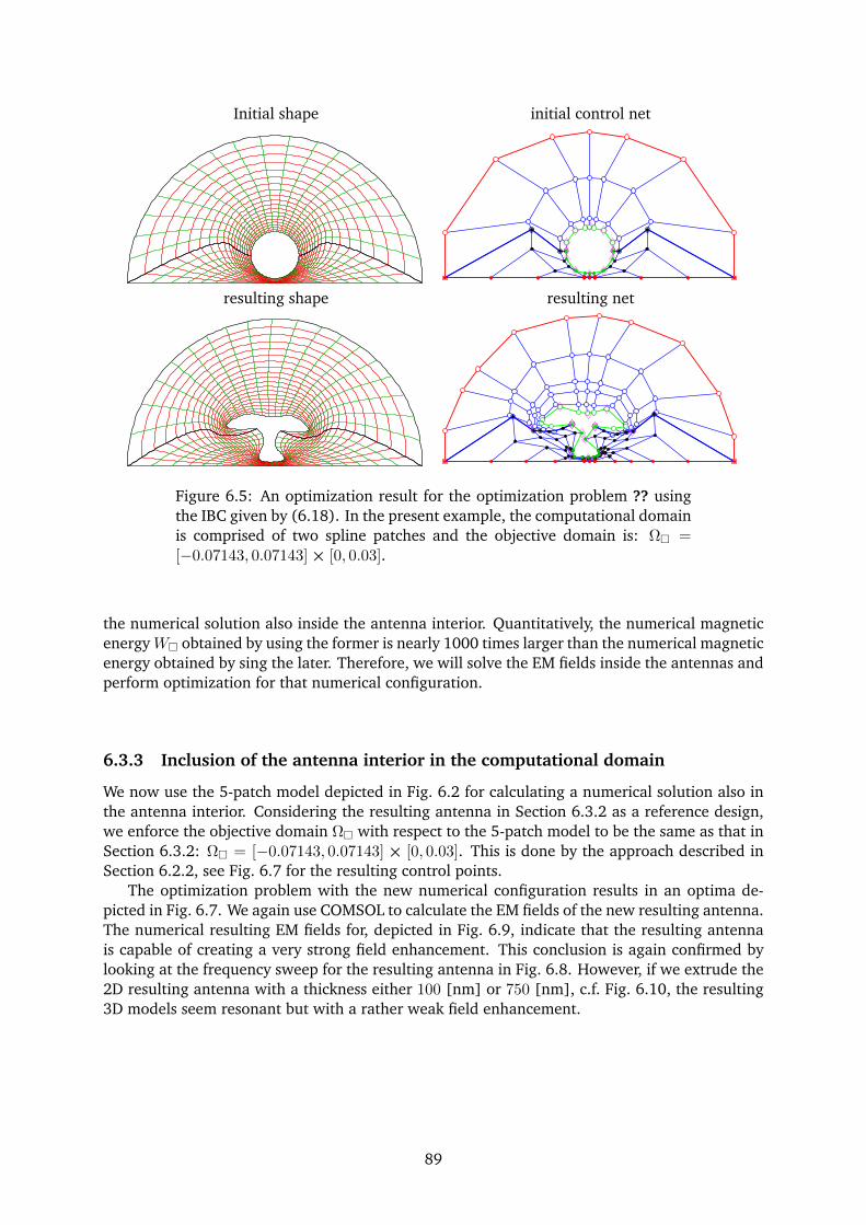
Initial shape initial control net
resulting shape resulting net
Figure 6.5: An optimization result for the optimization problem ?? usingthe IBC given by (6.18). In the present example, the computational domainis comprised of two spline patches and the objective domain is: Ω =[−0.07143, 0.07143]× [0, 0.03].
the numerical solution also inside the antenna interior. Quantitatively, the numerical magneticenergyW obtained by using the former is nearly 1000 times larger than the numerical magneticenergy obtained by sing the later. Therefore, we will solve the EM fields inside the antennas andperform optimization for that numerical configuration.
6.3.3 Inclusion of the antenna interior in the computational domain
We now use the 5-patch model depicted in Fig. 6.2 for calculating a numerical solution also inthe antenna interior. Considering the resulting antenna in Section 6.3.2 as a reference design,we enforce the objective domain Ω with respect to the 5-patch model to be the same as that inSection 6.3.2: Ω = [−0.07143, 0.07143]× [0, 0.03]. This is done by the approach described inSection 6.2.2, see Fig. 6.7 for the resulting control points.
The optimization problem with the new numerical configuration results in an optima de-picted in Fig. 6.7. We again use COMSOL to calculate the EM fields of the new resulting antenna.The numerical resulting EM fields for, depicted in Fig. 6.9, indicate that the resulting antennais capable of creating a very strong field enhancement. This conclusion is again confirmed bylooking at the frequency sweep for the resulting antenna in Fig. 6.8. However, if we extrude the2D resulting antenna with a thickness either 100 [nm] or 750 [nm], c.f. Fig. 6.10, the resulting3D models seem resonant but with a rather weak field enhancement.
89
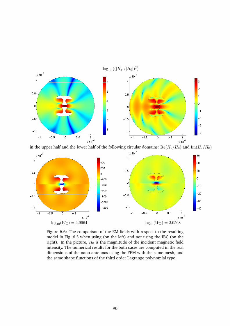
log10
((|Hz|/|H0|)2
)
in the upper half and the lower half of the following circular domains: Re(Hz/H0) and Im(Hz/H0)
log10(W) = 4.9964 log10(W) = 2.0568
Figure 6.6: The comparison of the EM fields with respect to the resultingmodel in Fig. 6.5 when using (on the left) and not using the IBC (on theright). In the picture, H0 is the magnitude of the incident magnetic fieldintensity. The numerical results for the both cases are computed in the realdimensions of the nano-antennas using the FEM with the same mesh, andthe same shape functions of the third order Lagrange polynomial type.
90
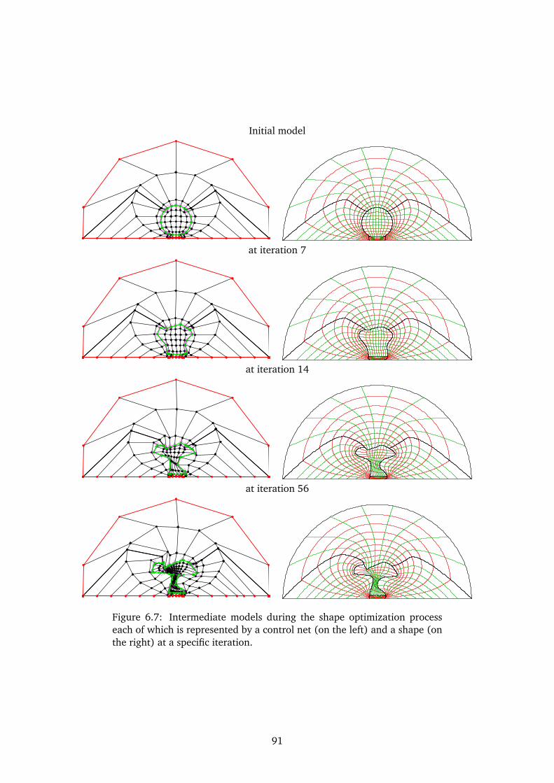
Initial model
at iteration 7
at iteration 14
at iteration 56
Figure 6.7: Intermediate models during the shape optimization processeach of which is represented by a control net (on the left) and a shape (onthe right) at a specific iteration.
91
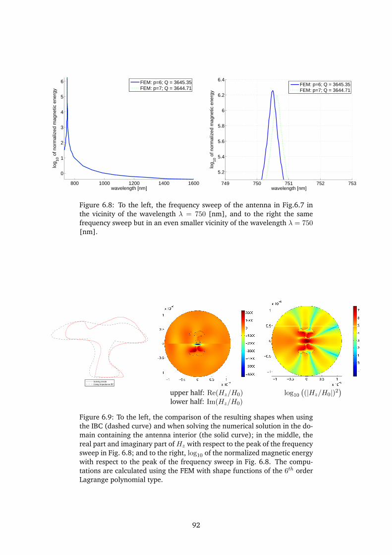
800 1000 1200 1400 1600
0
1
2
3
4
5
6
wavelength [nm]
log 10
of n
orm
aliz
ed m
agne
tic e
nerg
y
FEM: p=6; Q = 3645.35FEM: p=7; Q = 3644.71
749 750 751 752 753
5.2
5.4
5.6
5.8
6
6.2
6.4
wavelength [nm]
log 10
of n
orm
aliz
ed m
agne
tic e
nerg
y
FEM: p=6; Q = 3645.35FEM: p=7; Q = 3644.71
Figure 6.8: To the left, the frequency sweep of the antenna in Fig.6.7 inthe vicinity of the wavelength λ = 750 [nm], and to the right the samefrequency sweep but in an even smaller vicinity of the wavelength λ = 750[nm].
Solving insideUsing Impedance BC
upper half: Re(Hz/H0) log10
((|Hz/H0|)2
)
lower half: Im(Hz/H0)
Figure 6.9: To the left, the comparison of the resulting shapes when usingthe IBC (dashed curve) and when solving the numerical solution in the do-main containing the antenna interior (the solid curve); in the middle, thereal part and imaginary part ofHz with respect to the peak of the frequencysweep in Fig. 6.8; and to the right, log10 of the normalized magnetic energywith respect to the peak of the frequency sweep in Fig. 6.8. The compu-tations are calculated using the FEM with shape functions of the 6th orderLagrange polynomial type.
92
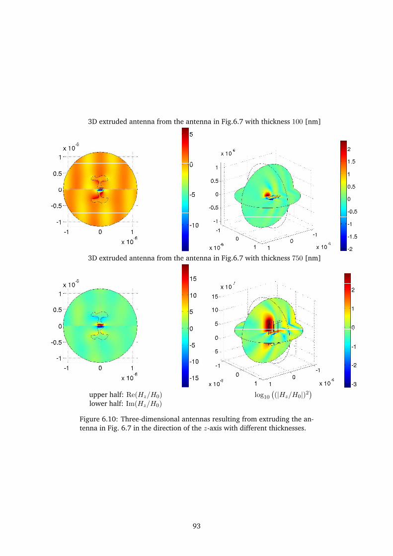
3D extruded antenna from the antenna in Fig.6.7 with thickness 100 [nm]
3D extruded antenna from the antenna in Fig.6.7 with thickness 750 [nm]
upper half: Re(Hz/H0) log10
((|Hz/H0|)2
)
lower half: Im(Hz/H0)
Figure 6.10: Three-dimensional antennas resulting from extruding the an-tenna in Fig. 6.7 in the direction of the z-axis with different thicknesses.
93

Part IV
Economical designs of magneticdensity separators
95

Chapter 7
Economical designs of magneticdensity separators using isogeometricanalysis and shape optimization
Nguyen D. M., A. Evgrafov, J. Gravesen, D. Lahaye, Economical designs of magnetic densityseparators using isogeometric analysis and shape optimization, in submission, 2012.
Abstract. We study the use of isogeometric analysis-based shape optimization for improvingan emerging magnetic density separation device. In particular, we look at a recently proposeddesign of such a device, which reduces the number of used electromagnets by a factor of twoor three compared to conventional designs. The use of a systematic design approach based onshape optimization allows us to further improve the performance of a known analytical design.The obtained results also show that the shapes of iron components have a very pronouncedeffect on the magnetic fields inside the device, which can be effectively utilized in differentengineering applications as well.
Keywords: Magnetic density separator; waste separator; shape optimization; isogeometric anal-ysis.
In collaboration with Domenico Lahaye, Delft Institute for Applied Mathematics, Delft Universityof Technology, Mekelweg 4, 2628 CD Delft, The Netherlands.
7.1 Introduction
In recent years, isogeometric analysis-based shape optimization (IGSO) has witnessed intensivedevelopments and has been applied in various engineering disciplines [11, 12, 9, 15, 16, 10].Such an interest is fueled by the fact that the incorporation of isogeometric analysis (IGA) into ashape optimization workflow allows one to represent complicated shapes with spline boundariesexactly and with relatively few parameters (control points), and perhaps even more importantly,import the optimized shapes back into a CAD system for manufacturing purposes [6, 7]. Theinvolvement of CAD systems also allows the utilizations of several well-studied and powerfultools for regularizing the shape parametrization and the geometries under consideration [8, 9,10].
Unfortunately, the incorporation of IGA into a shape optimization framework is not trivialdue to the fact that the parametrization control points need to be determined as smooth func-
97
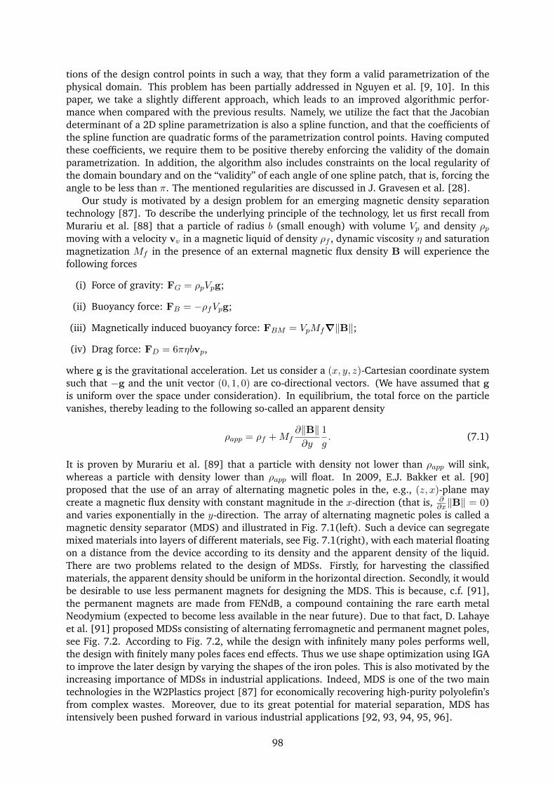
tions of the design control points in such a way, that they form a valid parametrization of thephysical domain. This problem has been partially addressed in Nguyen et al. [9, 10]. In thispaper, we take a slightly different approach, which leads to an improved algorithmic perfor-mance when compared with the previous results. Namely, we utilize the fact that the Jacobiandeterminant of a 2D spline parametrization is also a spline function, and that the coefficients ofthe spline function are quadratic forms of the parametrization control points. Having computedthese coefficients, we require them to be positive thereby enforcing the validity of the domainparametrization. In addition, the algorithm also includes constraints on the local regularity ofthe domain boundary and on the “validity” of each angle of one spline patch, that is, forcing theangle to be less than π. The mentioned regularities are discussed in J. Gravesen et al. [28].
Our study is motivated by a design problem for an emerging magnetic density separationtechnology [87]. To describe the underlying principle of the technology, let us first recall fromMurariu et al. [88] that a particle of radius b (small enough) with volume Vp and density ρpmoving with a velocity vv in a magnetic liquid of density ρf , dynamic viscosity η and saturationmagnetization Mf in the presence of an external magnetic flux density B will experience thefollowing forces
(i) Force of gravity: FG = ρpVpg;
(ii) Buoyancy force: FB = −ρfVpg;
(iii) Magnetically induced buoyancy force: FBM = VpMf∇‖B‖;
(iv) Drag force: FD = 6πηbvp,
where g is the gravitational acceleration. Let us consider a (x, y, z)-Cartesian coordinate systemsuch that −g and the unit vector (0, 1, 0) are co-directional vectors. (We have assumed that gis uniform over the space under consideration). In equilibrium, the total force on the particlevanishes, thereby leading to the following so-called an apparent density
ρapp = ρf +Mf∂‖B‖∂y
1
g. (7.1)
It is proven by Murariu et al. [89] that a particle with density not lower than ρapp will sink,whereas a particle with density lower than ρapp will float. In 2009, E.J. Bakker et al. [90]proposed that the use of an array of alternating magnetic poles in the, e.g., (z, x)-plane maycreate a magnetic flux density with constant magnitude in the x-direction (that is, ∂
∂x‖B‖ = 0)and varies exponentially in the y-direction. The array of alternating magnetic poles is called amagnetic density separator (MDS) and illustrated in Fig. 7.1(left). Such a device can segregatemixed materials into layers of different materials, see Fig. 7.1(right), with each material floatingon a distance from the device according to its density and the apparent density of the liquid.There are two problems related to the design of MDSs. Firstly, for harvesting the classifiedmaterials, the apparent density should be uniform in the horizontal direction. Secondly, it wouldbe desirable to use less permanent magnets for designing the MDS. This is because, c.f. [91],the permanent magnets are made from FENdB, a compound containing the rare earth metalNeodymium (expected to become less available in the near future). Due to that fact, D. Lahayeet al. [91] proposed MDSs consisting of alternating ferromagnetic and permanent magnet poles,see Fig. 7.2. According to Fig. 7.2, while the design with infinitely many poles performs well,the design with finitely many poles faces end effects. Thus we use shape optimization using IGAto improve the later design by varying the shapes of the iron poles. This is also motivated by theincreasing importance of MDSs in industrial applications. Indeed, MDS is one of the two maintechnologies in the W2Plastics project [87] for economically recovering high-purity polyolefin’sfrom complex wastes. Moreover, due to its great potential for material separation, MDS hasintensively been pushed forward in various industrial applications [92, 93, 94, 95, 96].
98
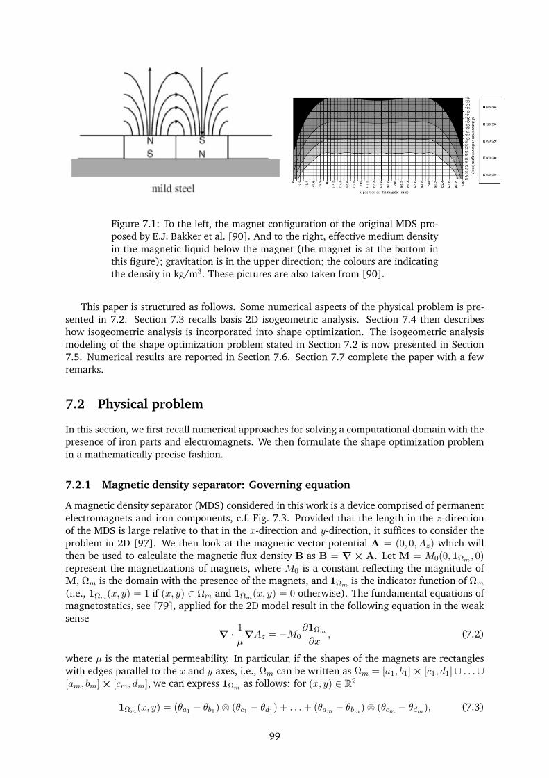
Figure 7.1: To the left, the magnet configuration of the original MDS pro-posed by E.J. Bakker et al. [90]. And to the right, effective medium densityin the magnetic liquid below the magnet (the magnet is at the bottom inthis figure); gravitation is in the upper direction; the colours are indicatingthe density in kg/m3. These pictures are also taken from [90].
This paper is structured as follows. Some numerical aspects of the physical problem is pre-sented in 7.2. Section 7.3 recalls basis 2D isogeometric analysis. Section 7.4 then describeshow isogeometric analysis is incorporated into shape optimization. The isogeometric analysismodeling of the shape optimization problem stated in Section 7.2 is now presented in Section7.5. Numerical results are reported in Section 7.6. Section 7.7 complete the paper with a fewremarks.
7.2 Physical problem
In this section, we first recall numerical approaches for solving a computational domain with thepresence of iron parts and electromagnets. We then formulate the shape optimization problemin a mathematically precise fashion.
7.2.1 Magnetic density separator: Governing equation
A magnetic density separator (MDS) considered in this work is a device comprised of permanentelectromagnets and iron components, c.f. Fig. 7.3. Provided that the length in the z-directionof the MDS is large relative to that in the x-direction and y-direction, it suffices to consider theproblem in 2D [97]. We then look at the magnetic vector potential A = (0, 0, Az) which willthen be used to calculate the magnetic flux density B as B = ∇×A. Let M = M0(0,1Ωm , 0)represent the magnetizations of magnets, where M0 is a constant reflecting the magnitude ofM, Ωm is the domain with the presence of the magnets, and 1Ωm is the indicator function of Ωm
(i.e., 1Ωm(x, y) = 1 if (x, y) ∈ Ωm and 1Ωm(x, y) = 0 otherwise). The fundamental equations ofmagnetostatics, see [79], applied for the 2D model result in the following equation in the weaksense
∇ · 1
µ∇Az = −M0
∂1Ωm
∂x, (7.2)
where µ is the material permeability. In particular, if the shapes of the magnets are rectangleswith edges parallel to the x and y axes, i.e., Ωm can be written as Ωm = [a1, b1]× [c1, d1] ∪ . . . ∪[am, bm]× [cm, dm], we can express 1Ωm as follows: for (x, y) ∈ R2
1Ωm(x, y) = (θa1 − θb1)⊗ (θc1 − θd1) + . . .+ (θam − θbm)⊗ (θcm − θdm), (7.3)
99
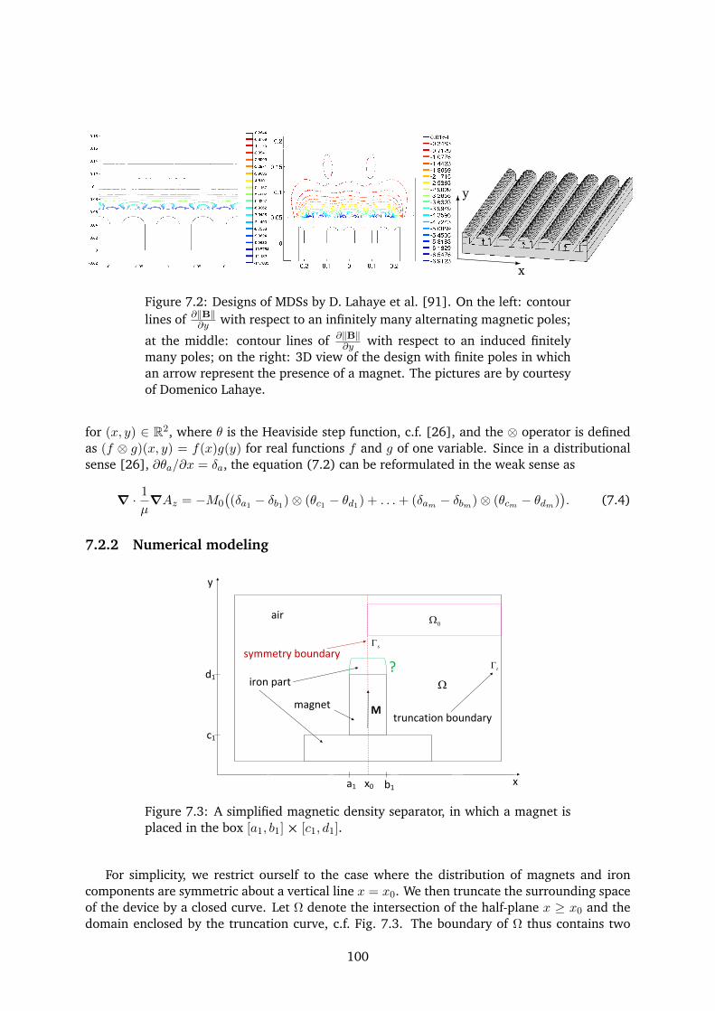
-
6
x
y
Figure 7.2: Designs of MDSs by D. Lahaye et al. [91]. On the left: contourlines of ∂‖B‖∂y with respect to an infinitely many alternating magnetic poles;
at the middle: contour lines of ∂‖B‖∂y with respect to an induced finitely
many poles; on the right: 3D view of the design with finite poles in whichan arrow represent the presence of a magnet. The pictures are by courtesyof Domenico Lahaye.
for (x, y) ∈ R2, where θ is the Heaviside step function, c.f. [26], and the ⊗ operator is definedas (f ⊗ g)(x, y) = f(x)g(y) for real functions f and g of one variable. Since in a distributionalsense [26], ∂θa/∂x = δa, the equation (7.2) can be reformulated in the weak sense as
∇ · 1
µ∇Az = −M0
((δa1 − δb1)⊗ (θc1 − θd1) + . . .+ (δam − δbm)⊗ (θcm − θdm)
). (7.4)
7.2.2 Numerical modeling
a1 b1
c1
d1
M
s
t
iron part
magnet
symmetry boundary
truncation boundary
?
air0
x0 x
y
Figure 7.3: A simplified magnetic density separator, in which a magnet isplaced in the box [a1, b1]× [c1, d1].
For simplicity, we restrict ourself to the case where the distribution of magnets and ironcomponents are symmetric about a vertical line x = x0. We then truncate the surrounding spaceof the device by a closed curve. Let Ω denote the intersection of the half-plane x ≥ x0 and thedomain enclosed by the truncation curve, c.f. Fig. 7.3. The boundary of Ω thus contains two
100
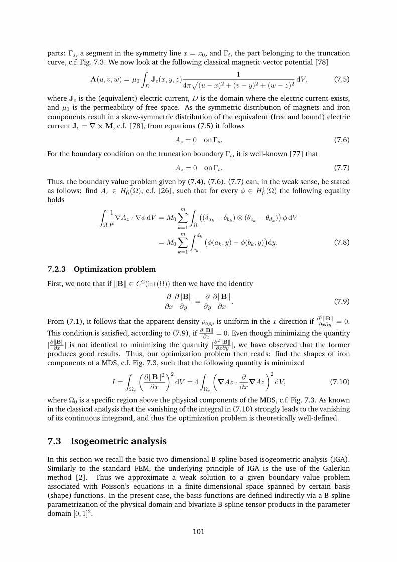
parts: Γs, a segment in the symmetry line x = x0, and Γt, the part belonging to the truncationcurve, c.f. Fig. 7.3. We now look at the following classical magnetic vector potential [78]
A(u, v, w) = µ0
∫
DJe(x, y, z)
1
4π√
(u− x)2 + (v − y)2 + (w − z)2dV, (7.5)
where Je is the (equivalent) electric current, D is the domain where the electric current exists,and µ0 is the permeability of free space. As the symmetric distribution of magnets and ironcomponents result in a skew-symmetric distribution of the equivalent (free and bound) electriccurrent Je = ∇×M, c.f. [78], from equations (7.5) it follows
Az = 0 on Γs. (7.6)
For the boundary condition on the truncation boundary Γt, it is well-known [77] that
Az = 0 on Γt. (7.7)
Thus, the boundary value problem given by (7.4), (7.6), (7.7) can, in the weak sense, be statedas follows: find Az ∈ H1
0 (Ω), c.f. [26], such that for every φ ∈ H10 (Ω) the following equality
holds∫
Ω
1
µ∇Az · ∇φ dV = M0
m∑
k=1
∫
Ω
((δak − δbk)⊗ (θck − θdk)
)φ dV
= M0
m∑
k=1
∫ dk
ck
(φ(ak, y)− φ(bk, y)
)dy. (7.8)
7.2.3 Optimization problem
First, we note that if ‖B‖ ∈ C2(int(Ω)) then we have the identity
∂
∂x
∂‖B‖∂y
=∂
∂y
∂‖B‖∂x
. (7.9)
From (7.1), it follows that the apparent density ρapp is uniform in the x-direction if ∂2‖B‖∂x∂y = 0.
This condition is satisfied, according to (7.9), if ∂‖B‖∂x = 0. Even though minimizing the quantity
|∂‖B‖∂x | is not identical to minimizing the quantity |∂2‖B‖∂x∂y |, we have observed that the formerproduces good results. Thus, our optimization problem then reads: find the shapes of ironcomponents of a MDS, c.f. Fig. 7.3, such that the following quantity is minimized
I =
∫
Ωo
(∂‖B‖2∂x
)2
dV = 4
∫
Ωo
(∇Az · ∂
∂x∇Az
)2
dV, (7.10)
where Ω0 is a specific region above the physical components of the MDS, c.f. Fig. 7.3. As knownin the classical analysis that the vanishing of the integral in (7.10) strongly leads to the vanishingof its continuous integrand, and thus the optimization problem is theoretically well-defined.
7.3 Isogeometric analysis
In this section we recall the basic two-dimensional B-spline based isogeometric analysis (IGA).Similarly to the standard FEM, the underlying principle of IGA is the use of the Galerkinmethod [2]. Thus we approximate a weak solution to a given boundary value problemassociated with Poisson’s equations in a finite-dimensional space spanned by certain basis(shape) functions. In the present case, the basis functions are defined indirectly via a B-splineparametrization of the physical domain and bivariate B-spline tensor products in the parameterdomain [0, 1]2.
101
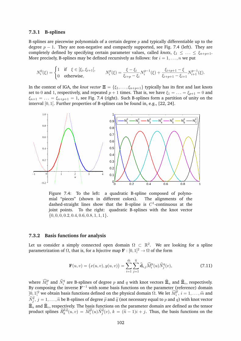
7.3.1 B-splines
B-splines are piecewise polynomials of a certain degree p and typically differentiable up to thedegree p − 1. They are non-negative and compactly supported, see Fig. 7.4 (left). They arecompletely defined by specifying certain parameter values, called knots, ξ1 ≤ . . . ≤ ξn+p+1.More precisely, B-splines may be defined recursively as follows: for i = 1, . . . , n we put
N0i (ξ) =
1 if ξ ∈ [ξi, ξi+1[,
0 otherwise,Npi (ξ) =
ξ − ξiξi+p − ξi
Np−1i (ξ) +
ξi+p+1 − ξξi+p+1 − ξi+1
Np−1i+1 (ξ).
In the context of IGA, the knot vector Ξ = ξ1, . . . , ξn+p+1 typically has its first and last knotsset to 0 and 1, respectively, and repeated p+ 1 times. That is, we have ξ1 = . . . = ξp+1 = 0 andξn+1 = . . . = ξn+p+1 = 1, see Fig. 7.4 (right). Such B-splines form a partition of unity on theinterval [0, 1[. Further properties of B-splines can be found in, e.g., [22, 24].
0 0.2 0.4 0.6 0.8 10
0.1
0.2
0.3
0.4
0.5
0.6
0.7
0.8
0.9
1
N21
N22
N23
N24
N25
N26
N27
Figure 7.4: To the left: a quadratic B-spline composed of polyno-mial “pieces” (shown in different colors). The alignments of thedashed-straight lines show that the B-spline is C1-continuous at thejoint points. To the right: quadratic B-splines with the knot vector0, 0, 0, 0.2, 0.4, 0.6, 0.8, 1, 1, 1.
7.3.2 Basis functions for analysis
Let us consider a simply connected open domain Ω ⊂ R2. We are looking for a splineparametrization of Ω, that is, for a bijective map F : [0, 1]2 → Ω of the form
F(u, v) =(x(u, v), y(u, v)
)=
m∑
i=1
n∑
j=1
di,jMpi (u)N q
j (v), (7.11)
where Mpi and N q
i are B-splines of degree p and q with knot vectors Ξu and Ξv, respectively.By composing the inverse F−1 with some basis functions on the parameter (reference) domain]0, 1[2 we obtain basis functions defined on the physical domain Ω. We let M p
i , i = 1, . . . , m andN qj , j = 1, . . . , n be B-splines of degree p and q (not necessary equal to p and q) with knot vector
Ξu and Ξv, respectively. The basis functions on the parameter domain are defined as the tensorproduct splines Rp,qk (u, v) = M p
i (u)N qj (v), k = (n − 1)i + j. Thus, the basis functions on the
102
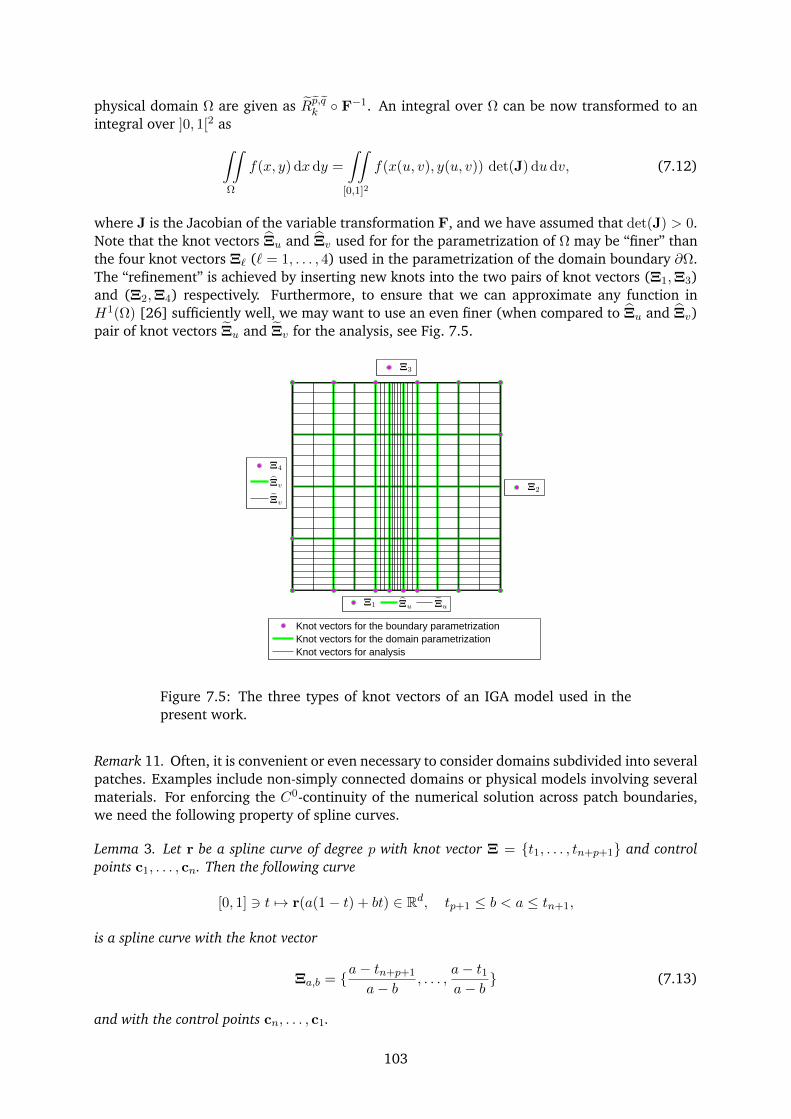
physical domain Ω are given as Rp,qk F−1. An integral over Ω can be now transformed to anintegral over ]0, 1[2 as
∫∫
Ω
f(x, y) dx dy =
∫∫
[0,1]2
f(x(u, v), y(u, v)) det(J) dudv, (7.12)
where J is the Jacobian of the variable transformation F, and we have assumed that det(J) > 0.Note that the knot vectors Ξu and Ξv used for for the parametrization of Ω may be “finer” thanthe four knot vectors Ξ` (` = 1, . . . , 4) used in the parametrization of the domain boundary ∂Ω.The “refinement” is achieved by inserting new knots into the two pairs of knot vectors (Ξ1,Ξ3)and (Ξ2,Ξ4) respectively. Furthermore, to ensure that we can approximate any function inH1(Ω) [26] sufficiently well, we may want to use an even finer (when compared to Ξu and Ξv)pair of knot vectors Ξu and Ξv for the analysis, see Fig. 7.5.
Ξ1 Ξu Ξu
Ξ3
Ξ2
Ξ4
Ξv
Ξv
Knot vectors for the boundary parametrizationKnot vectors for the domain parametrizationKnot vectors for analysis
Figure 7.5: The three types of knot vectors of an IGA model used in thepresent work.
Remark 11. Often, it is convenient or even necessary to consider domains subdivided into severalpatches. Examples include non-simply connected domains or physical models involving severalmaterials. For enforcing the C0-continuity of the numerical solution across patch boundaries,we need the following property of spline curves.
Lemma 3. Let r be a spline curve of degree p with knot vector Ξ = t1, . . . , tn+p+1 and controlpoints c1, . . . , cn. Then the following curve
[0, 1] 3 t 7→ r(a(1− t) + bt) ∈ Rd, tp+1 ≤ b < a ≤ tn+1,
is a spline curve with the knot vector
Ξa,b = a− tn+p+1
a− b , . . . ,a− t1a− b (7.13)
and with the control points cn, . . . , c1.
103
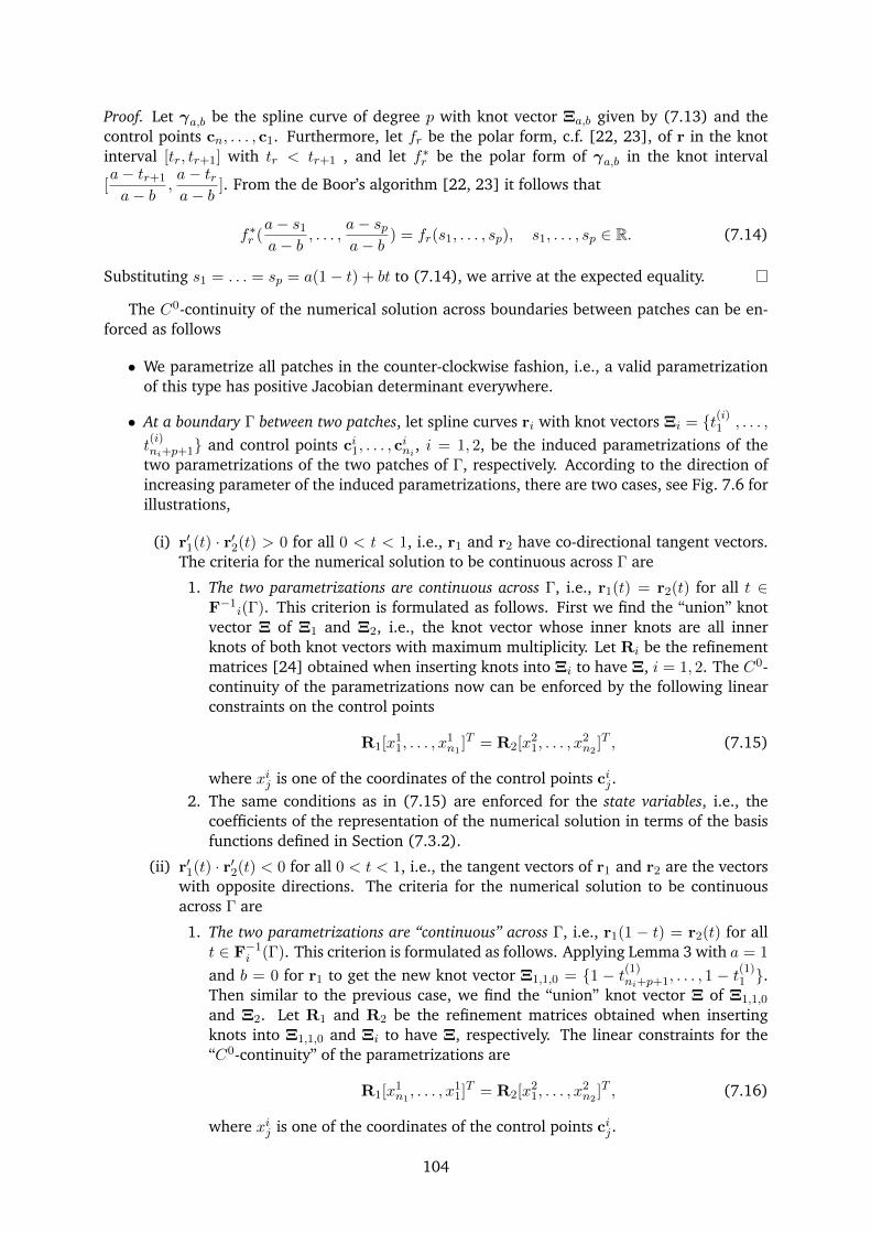
Proof. Let γa,b be the spline curve of degree p with knot vector Ξa,b given by (7.13) and thecontrol points cn, . . . , c1. Furthermore, let fr be the polar form, c.f. [22, 23], of r in the knotinterval [tr, tr+1] with tr < tr+1 , and let f∗r be the polar form of γa,b in the knot interval
[a− tr+1
a− b ,a− tra− b ]. From the de Boor’s algorithm [22, 23] it follows that
f∗r (a− s1
a− b , . . . ,a− spa− b ) = fr(s1, . . . , sp), s1, . . . , sp ∈ R. (7.14)
Substituting s1 = . . . = sp = a(1− t) + bt to (7.14), we arrive at the expected equality.
The C0-continuity of the numerical solution across boundaries between patches can be en-forced as follows
• We parametrize all patches in the counter-clockwise fashion, i.e., a valid parametrizationof this type has positive Jacobian determinant everywhere.
• At a boundary Γ between two patches, let spline curves ri with knot vectors Ξi = t(i)1 , . . . ,
t(i)ni+p+1 and control points ci1, . . . , c
ini , i = 1, 2, be the induced parametrizations of the
two parametrizations of the two patches of Γ, respectively. According to the direction ofincreasing parameter of the induced parametrizations, there are two cases, see Fig. 7.6 forillustrations,
(i) r′1(t) · r′2(t) > 0 for all 0 < t < 1, i.e., r1 and r2 have co-directional tangent vectors.The criteria for the numerical solution to be continuous across Γ are
1. The two parametrizations are continuous across Γ, i.e., r1(t) = r2(t) for all t ∈F−1
i(Γ). This criterion is formulated as follows. First we find the “union” knotvector Ξ of Ξ1 and Ξ2, i.e., the knot vector whose inner knots are all innerknots of both knot vectors with maximum multiplicity. Let Ri be the refinementmatrices [24] obtained when inserting knots into Ξi to have Ξ, i = 1, 2. The C0-continuity of the parametrizations now can be enforced by the following linearconstraints on the control points
R1[x11, . . . , x
1n1
]T = R2[x21, . . . , x
2n2
]T , (7.15)
where xij is one of the coordinates of the control points cij .2. The same conditions as in (7.15) are enforced for the state variables, i.e., the
coefficients of the representation of the numerical solution in terms of the basisfunctions defined in Section (7.3.2).
(ii) r′1(t) · r′2(t) < 0 for all 0 < t < 1, i.e., the tangent vectors of r1 and r2 are the vectorswith opposite directions. The criteria for the numerical solution to be continuousacross Γ are
1. The two parametrizations are “continuous” across Γ, i.e., r1(1 − t) = r2(t) for allt ∈ F−1
i (Γ). This criterion is formulated as follows. Applying Lemma 3 with a = 1
and b = 0 for r1 to get the new knot vector Ξ1,1,0 = 1 − t(1)ni+p+1, . . . , 1 − t
(1)1 .
Then similar to the previous case, we find the “union” knot vector Ξ of Ξ1,1,0
and Ξ2. Let R1 and R2 be the refinement matrices obtained when insertingknots into Ξ1,1,0 and Ξi to have Ξ, respectively. The linear constraints for the“C0-continuity” of the parametrizations are
R1[x1n1, . . . , x1
1]T = R2[x21, . . . , x
2n2
]T , (7.16)
where xij is one of the coordinates of the control points cij .
104
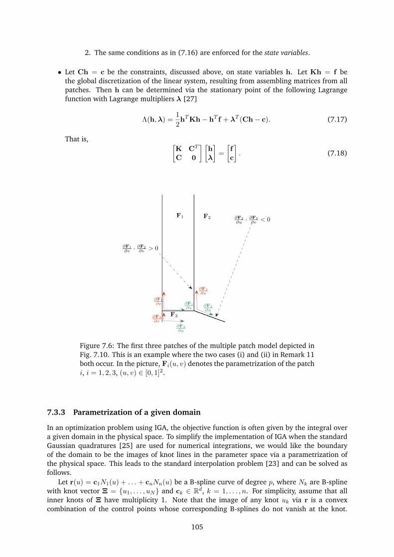
2. The same conditions as in (7.16) are enforced for the state variables.
• Let Ch = c be the constraints, discussed above, on state variables h. Let Kh = f bethe global discretization of the linear system, resulting from assembling matrices from allpatches. Then h can be determined via the stationary point of the following Lagrangefunction with Lagrange multipliers λ [27]
Λ(h,λ) =1
2hTKh− hT f + λT (Ch− c). (7.17)
That is, [K CT
C 0
] [hλ
]=
[fc
]. (7.18)
∂F2
∂uF3
∂F3
∂u
∂F2
∂v
∂F1
∂u
∂F1
∂v
∂F3
∂v
F2F1 ∂F2
∂u · ∂F3
∂v < 0
∂F1
∂v · ∂F2
∂v > 0
Figure 7.6: The first three patches of the multiple patch model depicted inFig. 7.10. This is an example where the two cases (i) and (ii) in Remark 11both occur. In the picture, Fi(u, v) denotes the parametrization of the patchi, i = 1, 2, 3, (u, v) ∈ [0, 1]2.
7.3.3 Parametrization of a given domain
In an optimization problem using IGA, the objective function is often given by the integral overa given domain in the physical space. To simplify the implementation of IGA when the standardGaussian quadratures [25] are used for numerical integrations, we would like the boundaryof the domain to be the images of knot lines in the parameter space via a parametrization ofthe physical space. This leads to the standard interpolation problem [23] and can be solved asfollows.
Let r(u) = c1N1(u) + . . . + cnNn(u) be a B-spline curve of degree p, where Nk are B-splinewith knot vector Ξ = u1, . . . , uN and ck ∈ Rd, k = 1, . . . , n. For simplicity, assume that allinner knots of Ξ have multiplicity 1. Note that the image of any knot uk via r is a convexcombination of the control points whose corresponding B-splines do not vanish at the knot.
105
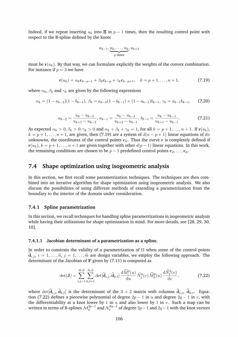
Indeed, if we repeat inserting uk into Ξ in p − 1 times, then the resulting control point withrespect to the B-spline defined by the knots
uk−1, uk, . . . , uk︸ ︷︷ ︸p times
, uk+1
must be r(uk). By that way, we can formulate explicitly the weights of the convex combination.For instance if p = 3 we have
r(uk) = αkck−p−1 + βkck−p + γkck−p+1, k = p+ 1, . . . , n+ 1, (7.19)
where αk, βk and γk are given by the following expressions
αk = (1− ak−2)(1− bk−1), βk = ak−2(1− bk−1) + (1− ak−1)bk−1, γk = ak−1bk−1, (7.20)
ak−2 =uk − uk−2
uk+1 − uk−2, ak−1 =
uk − uk−1
uk+2 − uk−1, bk−1 =
uk − uk−1
uk+1 − uk−1. (7.21)
As expected αk > 0, βk > 0, γk > 0 and αk + βk + γk = 1, for all k = p + 1, . . . , n + 1. If r(uk),k = p + 1, . . . , n + 1, are given, then (7.19) are a system of d(n − p + 1) linear equations of dnunknowns, the coordinates of the control points ck. Thus the curve r is completely defined ifr(uk), k = p+ 1, . . . , n+ 1 are given together with other d(p− 1) linear equations. In this work,the remaining conditions are chosen to be p− 1 predefined control points c2, . . . , cp.
7.4 Shape optimization using isogeometric analysis
In this section, we first recall some parametrization techniques. The techniques are then com-bined into an iterative algorithm for shape optimization using isogeometric analysis. We alsodiscuss the possibilities of using different methods of extending a parametrization from theboundary to the interior of the domain under consideration.
7.4.1 Spline parametrization
In this section, we recall techniques for handling spline parametrizations in isogeometric analysiswhile having their utilizations for shape optimization in mind. For more details, see [28, 29, 30,10].
7.4.1.1 Jacobian determinant of a parametrization as a spline.
In order to constrain the validity of a parametrization of Ω when some of the control pointsdi,j , i = 1, . . . , n, j = 1, . . . , m are design variables, we employ the following approach. Thedeterminant of the Jacobian of F given by (7.11) is computed as
det(J) =
m,n∑
i,j=1
m,n∑
k,`=1
det[di,j , dk,`]dMp
i (u)
duN qj (v) Mp
k (u)dN q
` (v)
dv, (7.22)
where det[di,j , dk,`] is the determinant of the 2 × 2 matrix with columns di,j , dk,`. Equa-tion (7.22) defines a piecewise polynomial of degree 2p − 1 in u and degree 2q − 1 in v, withthe differentiability at a knot lower by 1 in u and also lower by 1 in v. Such a map can bewritten in terms of B-splinesM2p−1
k and N 2q−1` of degree 2p−1 and 2q−1 with the knot vectors
106
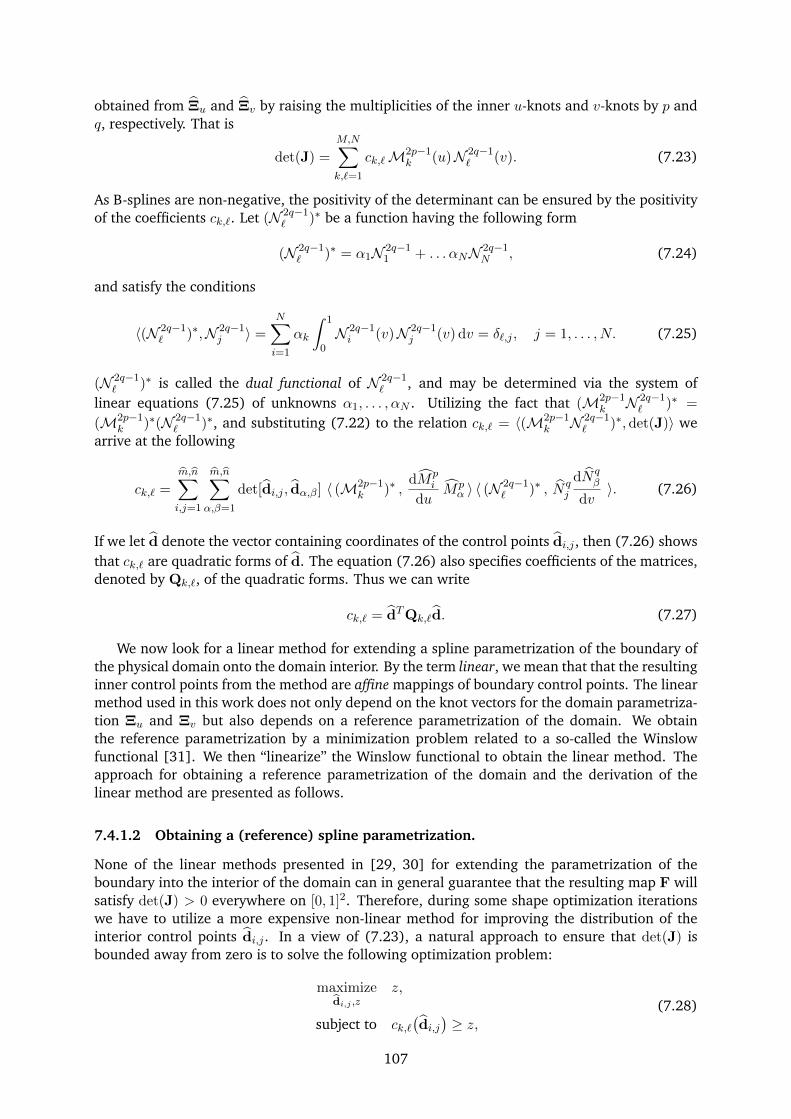
obtained from Ξu and Ξv by raising the multiplicities of the inner u-knots and v-knots by p andq, respectively. That is
det(J) =
M,N∑
k,`=1
ck,`M2p−1k (u)N 2q−1
` (v). (7.23)
As B-splines are non-negative, the positivity of the determinant can be ensured by the positivityof the coefficients ck,`. Let (N 2q−1
` )∗ be a function having the following form
(N 2q−1` )∗ = α1N 2q−1
1 + . . . αNN 2q−1N , (7.24)
and satisfy the conditions
〈(N 2q−1` )∗,N 2q−1
j 〉 =N∑
i=1
αk
∫ 1
0N 2q−1i (v)N 2q−1
j (v) dv = δ`,j , j = 1, . . . , N. (7.25)
(N 2q−1` )∗ is called the dual functional of N 2q−1
` , and may be determined via the system oflinear equations (7.25) of unknowns α1, . . . , αN . Utilizing the fact that (M2p−1
k N 2q−1` )∗ =
(M2p−1k )∗(N 2q−1
` )∗, and substituting (7.22) to the relation ck,` = 〈(M2p−1k N 2q−1
` )∗, det(J)〉 wearrive at the following
ck,` =
m,n∑
i,j=1
m,n∑
α,β=1
det[di,j , dα,β] 〈 (M2p−1k )∗ ,
dMpi
duMpα 〉 〈 (N 2q−1
` )∗ , N qj
dN qβ
dv〉. (7.26)
If we let d denote the vector containing coordinates of the control points di,j , then (7.26) showsthat ck,` are quadratic forms of d. The equation (7.26) also specifies coefficients of the matrices,denoted by Qk,`, of the quadratic forms. Thus we can write
ck,` = dTQk,`d. (7.27)
We now look for a linear method for extending a spline parametrization of the boundary ofthe physical domain onto the domain interior. By the term linear, we mean that that the resultinginner control points from the method are affine mappings of boundary control points. The linearmethod used in this work does not only depend on the knot vectors for the domain parametriza-tion Ξu and Ξv but also depends on a reference parametrization of the domain. We obtainthe reference parametrization by a minimization problem related to a so-called the Winslowfunctional [31]. We then “linearize” the Winslow functional to obtain the linear method. Theapproach for obtaining a reference parametrization of the domain and the derivation of thelinear method are presented as follows.
7.4.1.2 Obtaining a (reference) spline parametrization.
None of the linear methods presented in [29, 30] for extending the parametrization of theboundary into the interior of the domain can in general guarantee that the resulting map F willsatisfy det(J) > 0 everywhere on [0, 1]2. Therefore, during some shape optimization iterationswe have to utilize a more expensive non-linear method for improving the distribution of theinterior control points di,j . In a view of (7.23), a natural approach to ensure that det(J) isbounded away from zero is to solve the following optimization problem:
maximizedi,j ,z
z,
subject to ck,`(di,j)≥ z,
(7.28)
107
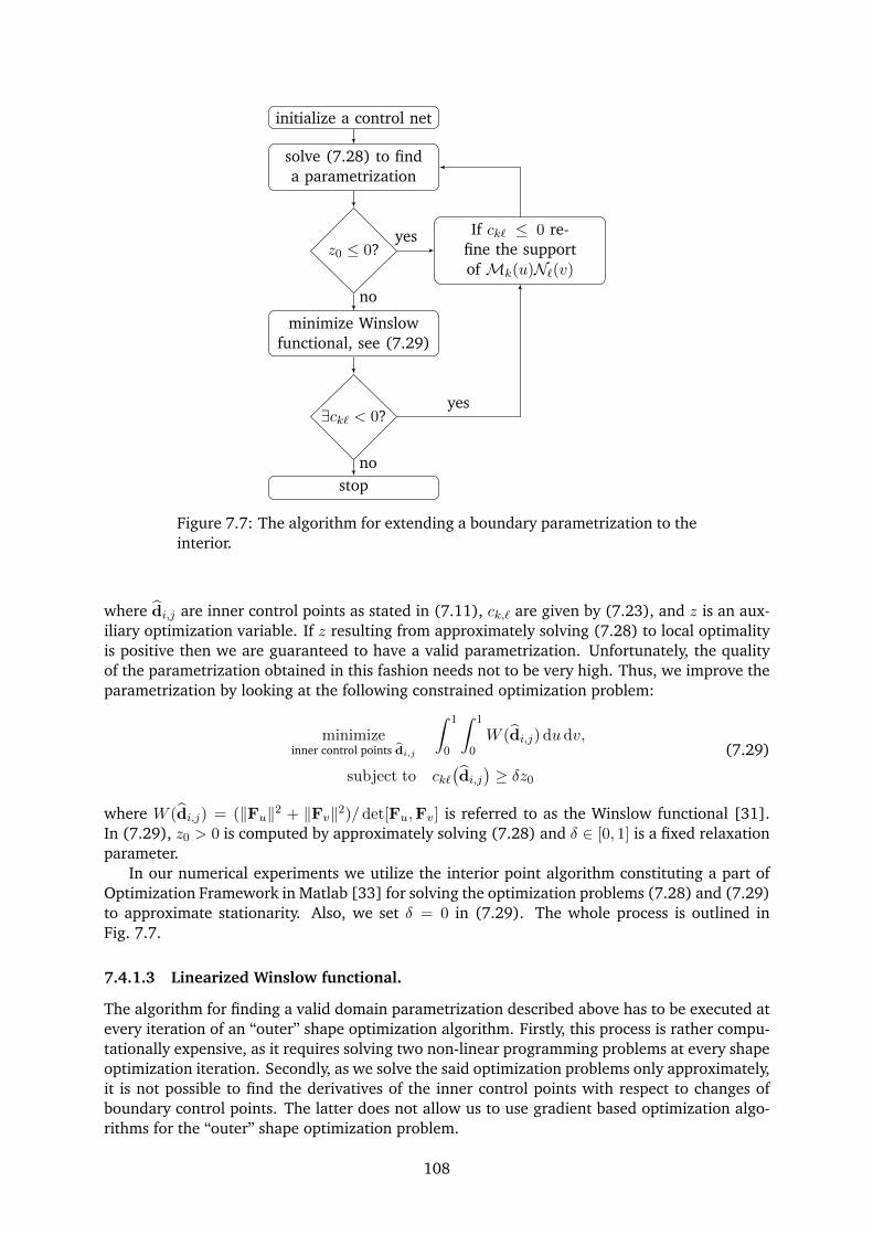
initialize a control net
solve (7.28) to finda parametrization
z0 ≤ 0?
minimize Winslowfunctional, see (7.29)
If ck` ≤ 0 re-fine the supportof Mk(u)N`(v)
∃ck` < 0?
stop
yes
no
yes
no
Figure 7.7: The algorithm for extending a boundary parametrization to theinterior.
where di,j are inner control points as stated in (7.11), ck,` are given by (7.23), and z is an aux-iliary optimization variable. If z resulting from approximately solving (7.28) to local optimalityis positive then we are guaranteed to have a valid parametrization. Unfortunately, the qualityof the parametrization obtained in this fashion needs not to be very high. Thus, we improve theparametrization by looking at the following constrained optimization problem:
minimizeinner control points di,j
∫ 1
0
∫ 1
0W (di,j) dudv,
subject to ck`(di,j)≥ δz0
(7.29)
where W (di,j) = (‖Fu‖2 + ‖Fv‖2)/ det[Fu,Fv] is referred to as the Winslow functional [31].In (7.29), z0 > 0 is computed by approximately solving (7.28) and δ ∈ [0, 1] is a fixed relaxationparameter.
In our numerical experiments we utilize the interior point algorithm constituting a part ofOptimization Framework in Matlab [33] for solving the optimization problems (7.28) and (7.29)to approximate stationarity. Also, we set δ = 0 in (7.29). The whole process is outlined inFig. 7.7.
7.4.1.3 Linearized Winslow functional.
The algorithm for finding a valid domain parametrization described above has to be executed atevery iteration of an “outer” shape optimization algorithm. Firstly, this process is rather compu-tationally expensive, as it requires solving two non-linear programming problems at every shapeoptimization iteration. Secondly, as we solve the said optimization problems only approximately,it is not possible to find the derivatives of the inner control points with respect to changes ofboundary control points. The latter does not allow us to use gradient based optimization algo-rithms for the “outer” shape optimization problem.
108
To avoid this difficulty, we linearize the process of computing a domain parametrization.Namely, we can Taylor-expand the Winslow functional as
W(d) =
∫∫
ΩW (d) dudv ≈ W(d0) + (d− d0)T G(d0) +
1
2(d− d0)T H(d0) (d− d0), (7.30)
where d is a vector with all control points di,j , d0 is the control points for a referenceparametrization obtained by solving (7.29), and G and H are the gradient and Hessian ofW re-spectively. If we split the control points d = (d1 d2)T into the part d2 that is given (typically theboundary control points) and the part d1 that has to be determined (typically the inner controlpoints), then we can write (7.30) as
W(d) ≈ W(d0) +(d1 − d1,0 d2 − d2,0
)(G1
G2
)
+1
2
(d1 − d1,0 d2 − d2,0
)(H11 H12
H21 H22
)(d1 − d1,0
d2 − d2,0
). (7.31)
The minimum of the right hand side of (7.31) is obtained when d1 satisfies the linear equation
H11(d1 − d1,0) = −G1 −H12(d2 − d2,0). (7.32)
This gives us a fast method for computing the domain parametrization and its derivativeswith respect to the boundary control points. We use this method as long as we obtain avalid parametrization, but if the parametrization at some point fails the test described in Sec-tion 7.4.1.1 then we restart the “outer” shape optimization algorithm with a new referenceparametrization d0 found by the method described in Section 7.4.1.2.
The given control points d2 can further be split into the set of fixed control points df andcontrol points Rd obtained from the design variables (control points) d by knot insertion (re-finement).
7.4.2 Shape optimization algorithm
Let us consider the following shape optimization problem using isogeometric analysis
minimized∈Ωd
f(d) (7.33)
where Ωd ⊂ Rn is the space of design variables, and d are typically coordinates of boundarycontrol points of spline patches. We solve the problem by the following iterative algorithm
• Start the algorithm with a guess d0 ∈ int(Ωd).
• Let Ad0 and Bd0 be the matrices of an affine mapping that represent a linear method ofextending the parametrization from the boundary to the interior of the physical domain,i.e., it generates all control points d from d by the following relation
d(d) = Ad0d + Bd0 , d ∈ Ωd. (7.34)
Assume Ad0 and Bd0 satisfy the condition that d(d0) = Ad0d0+Bd0 corresponds to a validparametrization. Thus with a sufficient subdivision of the Jacobian determinant surface,c.f. (7.22), its representing control points ck,` given by (7.23) are positive. For simplicity letus assume that without further refinement, the control points ck,` are positive. Accordingto (7.27)
ck,`(d) = (Ad0d + Bd0)TQk,`(Ad0d + Bd0). (7.35)
The control points ck,` are obviously continuous functions of d, thus there exists a neigh-borhood Bd0 ⊂ Ωd0 of d0 such that
ck,`(d) > 0 ∀d ∈ Bd0 , ∀k, `. (7.36)
109
• We then would like to solve the following sub-optimization problem
d1 = argmind∈Bd0
f(d), (7.37)
where argmin denotes the argument of the minimum of a function. In practice, it is difficultto determine Bd0 , especially the “maximal” one, i.e., the largest neighborhood satisfying(7.36). Instead, we find d1 as the solution to the following problem
minimized∈Ωd
f(d), (7.38a)
such that ck,`(d) ≥ ε, (7.38b)
where ε is some positive constant. Note that the values and sensitivities of the constraints(7.38b) are very easy to compute using (7.35).
• Repeat the steps above by replacing d0 with d1, and stop when convergence.
Remark 12. We note that
(i) The linearized Winslow functional presented in Section 7.4.1.3 and the quasi-conformaldeformation [30] are among the methods that fulfill the condition related to (7.34).
(ii) In J. Gravesen et al. [28], any parametrization of a 2D B-spline patch with a corner havingangle more than π is invalid. Therefore, it is necessary to constrain the angles. Fortunately,they are already included in the constraints (7.38b) as those on the corner control pointsof the Jacobian determinant ensure the “validity” of the corresponding angles.
(iii) One problem of shape optimization using isogeometric analysis has been encounteredin fluid mechanics is the clustering of control points [28]. This requires some specialtreatment [28]. Interestingly, without extra efforts the algorithm above avoids this issue.Indeed, since the the boundary control points of the Jacobian determinant are constrainedto be positive, the boundary parametrization must be locally regular.
7.4.3 Multiple methods of extending parametrization from boundary to interior
For some problems, there are regions which can be parametrized in a simple and effective way.For such a case, it is not necessary to employ more complicated and expensive methods to extendthe parametrization from the boundaries to the interiors of those regions. Thus in general wecan have different linear parametrization extension methods for different regions. See Fig. 7.10and Fig. 7.13 for illustrations of the argument.
For the sake of deriving sensitivity later on and implementation, let us formulate the gen-eral configuration. Let Ω be a connected domain. Assume that according to parametrizationextension, Ω can be partitioned into N sub-domains Ωk, k = 1, . . . , N . Each sub-domains arecomprised of several B-spline patches. Let d be the design variable vector and dk be the controlpoint vector of ∂Ωk. The first task for the algorithm is to determine affine maps that sending dto dk as
dk = akd + bk. (7.39)
The next task will be to derive affine transformations that map dk to unknown inner controlpoints of Ωk, and therefore to the control point vector dk of Ωk
dk = Akdk + Bk = Akakd + Akbk + Bk. (7.40)
Note that the refinement matrices [24] obtained when inserting knots into the boundary knotvectors to have parametrization knot vectors are already taken into account in Ak. If for somesub-domain Ωk, the parametrization extension method used in this domain is guaranteed toresult in a valid parametrization then the constraints (7.38b) with respect to this domain shouldbe removed to reduce computational time consume.
110
7.5 Discretization and sensitivity analysis
Formulation of the discretization using isogeometric analysis are first presented. The sensitivityanalysis are then derived precisely.
7.5.1 Discretization
An approximation to the solution Az to the boundary value problem given by (7.4), (7.6), (7.7)is expanded in terms of the basis functions (see Section 7.3.2) as
Az =∑
k
hk (Rp,qk F−1) =[Rp,q1 F−1, . . . , Rp,qmn F−1
]h, (7.41)
where h contains all the coordinates of Az with respect to the selected basis. Substituting thisexpression into the weak form (7.8) and utilizing the basis functions as the test functions, wearrive at the following set of linear algebraic equations:
K h = f . (7.42)
Entries of the matrices entering (7.42) are with the help of (7.12) calculated as:
Kk` =
∫∫
[0,1]2
1
µ
(∇Rp,qk (u, v) J−1
)T ∇Rp,q` (u, v) J−1 det(J) dudv, (7.43a)
f` = M0
m∑
i=1
(∫
F−1(ai×[ci,di])Rp,q` ds−
∫
F−1(bi×[ci,di])Rp,q` ds
), (7.43b)
k, ` = 1, . . . , mn. In (7.43), J denotes the Jacobian of the parametrization F.
7.5.2 Sensitivity analysis
For convenience, let us first introduce the basis notations: F(u, v) = (x(u, v), y(u, v)) andF−1(x, y) = (u(x, y), v(x, y)). Let us now formulate the objective function given by (7.10).Differentiation of (7.41) gives
∇Az =[J−1 (∇Rp,q1 F−1), . . . ,J−1 (∇Rp,qmn F−1)
]h. (7.44)
Furthermore, note that by differentiating the identity J−1J = I, where I is the 2-by-2 identitymatrix, we get
∂
∂xJ−1 = −J−1
(∂J
∂uux +
∂J
∂vvx)J−1. (7.45)
Thus again from differentiating (7.44) with respect to x, it follows
∂
∂x∇Az =
[g1 F−1, . . . ,gmn F−1
]h, (7.46)
where
gk =J−1
det(J)
(H(Rp,qk )
[yv−yu
]− J−1
(∂J
∂uyv −
∂J
∂vyu)J−1∇Rp,qk
). (7.47)
In (7.47), H(f) is the Hessian of a real-valued function f : [0, 1]2 7→ R. The objective functionnow can be written as
I = 4
∫∫
F−1(Ω0)
([J−1∇Rp,q1 , . . . ,J−1∇Rp,qmn
]h ·[g1, . . . ,gmn
]h
)2
det(J) dudv. (7.48)
111
To facilitate sensitivity analysis, we keep the parametrization of Ω0 fixed, i.e., independent fromchanges of design control points, see Fig. 7.11. Thus to calculate the sensitivity ∂I
∂diof I, given
by (7.48), with respect to a design control point coordinate di, we only need to determine ∂h∂di
.
Differentiating both sides of (7.42) and utilizing the fact that ∂f∂di
= 0, the partial derivative isin turn the solution to the following linear system
K∂h
di= −∂K
dih. (7.49)
In (7.49), the partial derivatives of K are calculated straightforwardly by differentiating (7.43).Finally, as we employ linear parametrization methods formulated in (7.40), the desired sensitiv-ities are
∂I
∂d= aT1 AT
1
∂I
∂d1
+ . . .+ aTNATN
∂I
∂dN. (7.50)
7.6 Numerical experiments
It has been noted in [91] that complex geometries of the design iron components make it diffi-cult to remove magnetic contaminants attracted to the device. We therefore only consider theordinates of the control points of the iron poles as design variables. Furthermore, as a standardin engineering, we consider log10(I) as the objective function for the shape optimization insteadof I given by (7.10). The relative permeabilities of air and iron are 1 and 1000, respectively. Themagnitude of the magnetization of the magnets is M0 = 106 [A/m].
For the content of this section, we first test all numerical settings including the shape opti-mization algorithm presented in Section 7.4.2, the choice of the fixed domain for optimizationand the choice of the objective function given by (7.10) in an example with known analyticalsolution. Then then perform shape optimization on different configurations.
7.6.1 A test problem
In this section we consider a simple shape optimization problem that inspired by D. Lahaye etal. [91]. For this, let us first look at the following harmonic function
u(x, y) = u0 cos(πx
λ)e−πyλ , u0 > 0, λ > 0. (7.51)
The geometry that adapts the above function to its solution should be the optimum of the opti-mization problem (7.10) since
∂
∂x‖B‖ =
∂
∂x‖(∂u∂y,−∂u
∂y, 0)‖ =
∂
∂x
(u0π
λe−πyλ)
= 0. (7.52)
Interestingly, the geometry can be derived analytically by observing that we can write the explicitformula for the level set of u with respect to a positive constant c, u(x, y) = c as
y =λ
πln cos(
πx
λ) +
λ
πlnu0
c, −λ
2< −(
λ
2− ε) ≤ x < λ
2− ε ≤ λ
2. (7.53)
In (7.53), as x approaches −λ2 or λ
2 , y approaches −∞, a positive constant ε is introduced totruncate the two singularities. That is, u(x, y) given by (7.51) is the solution to the followingDirichlet boundary value problem on a domain D with boundary components Γb, Γr, Γt, and Γlas depicted in Fig. 7.8
∆u = 0 in D (7.54a)
u = c on Γb (7.54b)
u = u0 cos(πx
λ)e−πyλ on Γl, Γr, and Γt (7.54c)
112
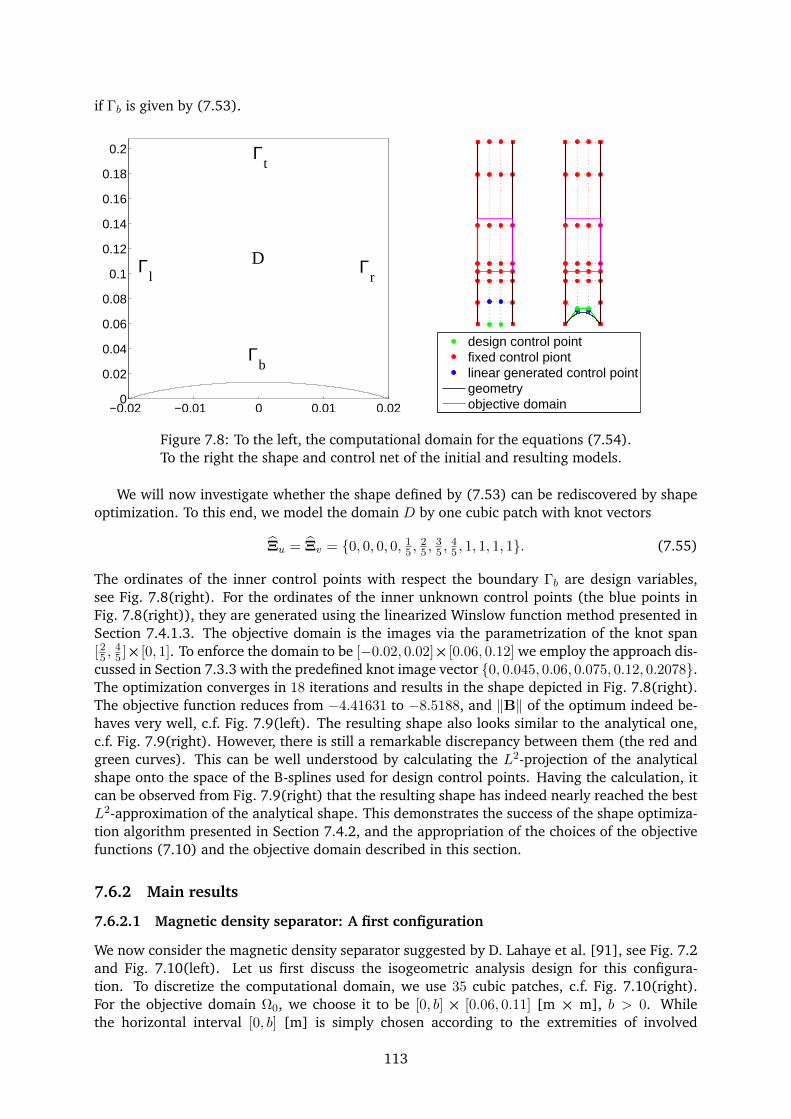
if Γb is given by (7.53).
−0.02 −0.01 0 0.01 0.020
0.02
0.04
0.06
0.08
0.1
0.12
0.14
0.16
0.18
0.2 Γt
Γl
Γr
Γb
D
design control pointfixed control piontlinear generated control pointgeometryobjective domain
Figure 7.8: To the left, the computational domain for the equations (7.54).To the right the shape and control net of the initial and resulting models.
We will now investigate whether the shape defined by (7.53) can be rediscovered by shapeoptimization. To this end, we model the domain D by one cubic patch with knot vectors
Ξu = Ξv = 0, 0, 0, 0, 15 ,
25 ,
35 ,
45 , 1, 1, 1, 1. (7.55)
The ordinates of the inner control points with respect the boundary Γb are design variables,see Fig. 7.8(right). For the ordinates of the inner unknown control points (the blue points inFig. 7.8(right)), they are generated using the linearized Winslow function method presented inSection 7.4.1.3. The objective domain is the images via the parametrization of the knot span[25 ,
45 ]×[0, 1]. To enforce the domain to be [−0.02, 0.02]×[0.06, 0.12] we employ the approach dis-
cussed in Section 7.3.3 with the predefined knot image vector 0, 0.045, 0.06, 0.075, 0.12, 0.2078.The optimization converges in 18 iterations and results in the shape depicted in Fig. 7.8(right).The objective function reduces from −4.41631 to −8.5188, and ‖B‖ of the optimum indeed be-haves very well, c.f. Fig. 7.9(left). The resulting shape also looks similar to the analytical one,c.f. Fig. 7.9(right). However, there is still a remarkable discrepancy between them (the red andgreen curves). This can be well understood by calculating the L2-projection of the analyticalshape onto the space of the B-splines used for design control points. Having the calculation, itcan be observed from Fig. 7.9(right) that the resulting shape has indeed nearly reached the bestL2-approximation of the analytical shape. This demonstrates the success of the shape optimiza-tion algorithm presented in Section 7.4.2, and the appropriation of the choices of the objectivefunctions (7.10) and the objective domain described in this section.
7.6.2 Main results
7.6.2.1 Magnetic density separator: A first configuration
We now consider the magnetic density separator suggested by D. Lahaye et al. [91], see Fig. 7.2and Fig. 7.10(left). Let us first discuss the isogeometric analysis design for this configura-tion. To discretize the computational domain, we use 35 cubic patches, c.f. Fig. 7.10(right).For the objective domain Ω0, we choose it to be [0, b] × [0.06, 0.11] [m × m], b > 0. Whilethe horizontal interval [0, b] [m] is simply chosen according to the extremities of involved
113
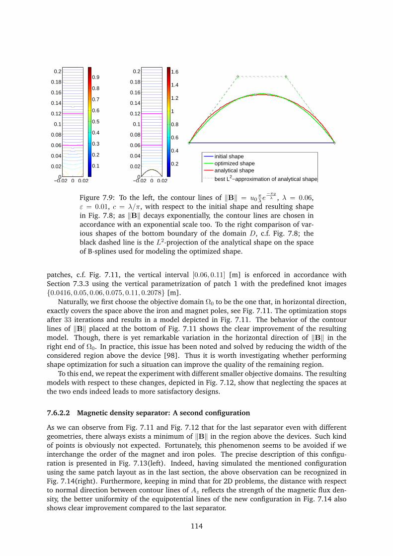
−0.02 0 0.020
0.02
0.04
0.06
0.08
0.1
0.12
0.14
0.16
0.18
0.2
0.1
0.2
0.3
0.4
0.5
0.6
0.7
0.8
0.9
−0.02 0 0.020
0.02
0.04
0.06
0.08
0.1
0.12
0.14
0.16
0.18
0.2
0.2
0.4
0.6
0.8
1
1.2
1.4
1.6
initial shapeoptimized shapeanalytical shape
best L2−approximation of analytical shape
Figure 7.9: To the left, the contour lines of ‖B‖ = u0πλe−πyλ , λ = 0.06,
ε = 0.01, c = λ/π, with respect to the initial shape and resulting shapein Fig. 7.8; as ‖B‖ decays exponentially, the contour lines are chosen inaccordance with an exponential scale too. To the right comparison of var-ious shapes of the bottom boundary of the domain D, c.f. Fig. 7.8; theblack dashed line is the L2-projection of the analytical shape on the spaceof B-splines used for modeling the optimized shape.
patches, c.f. Fig. 7.11, the vertical interval [0.06, 0.11] [m] is enforced in accordance withSection 7.3.3 using the vertical parametrization of patch 1 with the predefined knot images0.0416, 0.05, 0.06, 0.075, 0.11, 0.2078 [m].
Naturally, we first choose the objective domain Ω0 to be the one that, in horizontal direction,exactly covers the space above the iron and magnet poles, see Fig. 7.11. The optimization stopsafter 33 iterations and results in a model depicted in Fig. 7.11. The behavior of the contourlines of ‖B‖ placed at the bottom of Fig. 7.11 shows the clear improvement of the resultingmodel. Though, there is yet remarkable variation in the horizontal direction of ‖B‖ in theright end of Ω0. In practice, this issue has been noted and solved by reducing the width of theconsidered region above the device [98]. Thus it is worth investigating whether performingshape optimization for such a situation can improve the quality of the remaining region.
To this end, we repeat the experiment with different smaller objective domains. The resultingmodels with respect to these changes, depicted in Fig. 7.12, show that neglecting the spaces atthe two ends indeed leads to more satisfactory designs.
7.6.2.2 Magnetic density separator: A second configuration
As we can observe from Fig. 7.11 and Fig. 7.12 that for the last separator even with differentgeometries, there always exists a minimum of ‖B‖ in the region above the devices. Such kindof points is obviously not expected. Fortunately, this phenomenon seems to be avoided if weinterchange the order of the magnet and iron poles. The precise description of this configu-ration is presented in Fig. 7.13(left). Indeed, having simulated the mentioned configurationusing the same patch layout as in the last section, the above observation can be recognized inFig. 7.14(right). Furthermore, keeping in mind that for 2D problems, the distance with respectto normal direction between contour lines of Az reflects the strength of the magnetic flux den-sity, the better uniformity of the equipotential lines of the new configuration in Fig. 7.14 alsoshows clear improvement compared to the last separator.
114
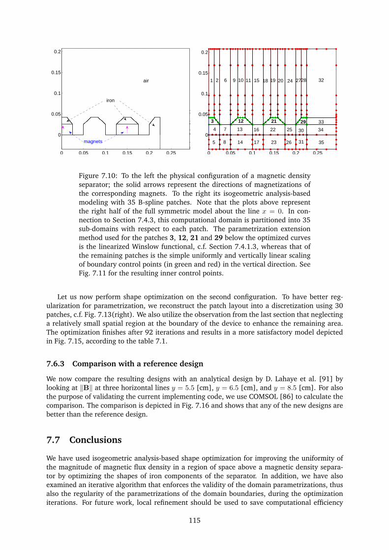
0 0.05 0.1 0.15 0.2 0.25
0
0.05
0.1
0.15
0.2
magnets
iron
air
0 0.05 0.1 0.15 0.2 0.25
0
0.05
0.1
0.15
0.2
1
3
4 7
292112
102 6 9 11 15 18 19 20 24 2728 32
33
13 16
171485 23
22
26
25 30
31
34
35
Figure 7.10: To the left the physical configuration of a magnetic densityseparator; the solid arrows represent the directions of magnetizations ofthe corresponding magnets. To the right its isogeometric analysis-basedmodeling with 35 B-spline patches. Note that the plots above representthe right half of the full symmetric model about the line x = 0. In con-nection to Section 7.4.3, this computational domain is partitioned into 35sub-domains with respect to each patch. The parametrization extensionmethod used for the patches 3, 12, 21 and 29 below the optimized curvesis the linearized Winslow functional, c.f. Section 7.4.1.3, whereas that ofthe remaining patches is the simple uniformly and vertically linear scalingof boundary control points (in green and red) in the vertical direction. SeeFig. 7.11 for the resulting inner control points.
Let us now perform shape optimization on the second configuration. To have better reg-ularization for parametrization, we reconstruct the patch layout into a discretization using 30patches, c.f. Fig. 7.13(right). We also utilize the observation from the last section that neglectinga relatively small spatial region at the boundary of the device to enhance the remaining area.The optimization finishes after 92 iterations and results in a more satisfactory model depictedin Fig. 7.15, according to the table 7.1.
7.6.3 Comparison with a reference design
We now compare the resulting designs with an analytical design by D. Lahaye et al. [91] bylooking at ‖B‖ at three horizontal lines y = 5.5 [cm], y = 6.5 [cm], and y = 8.5 [cm]. For alsothe purpose of validating the current implementing code, we use COMSOL [86] to calculate thecomparison. The comparison is depicted in Fig. 7.16 and shows that any of the new designs arebetter than the reference design.
7.7 Conclusions
We have used isogeometric analysis-based shape optimization for improving the uniformity ofthe magnitude of magnetic flux density in a region of space above a magnetic density separa-tor by optimizing the shapes of iron components of the separator. In addition, we have alsoexamined an iterative algorithm that enforces the validity of the domain parametrizations, thusalso the regularity of the parametrizations of the domain boundaries, during the optimizationiterations. For future work, local refinement should be used to save computational efficiency
115
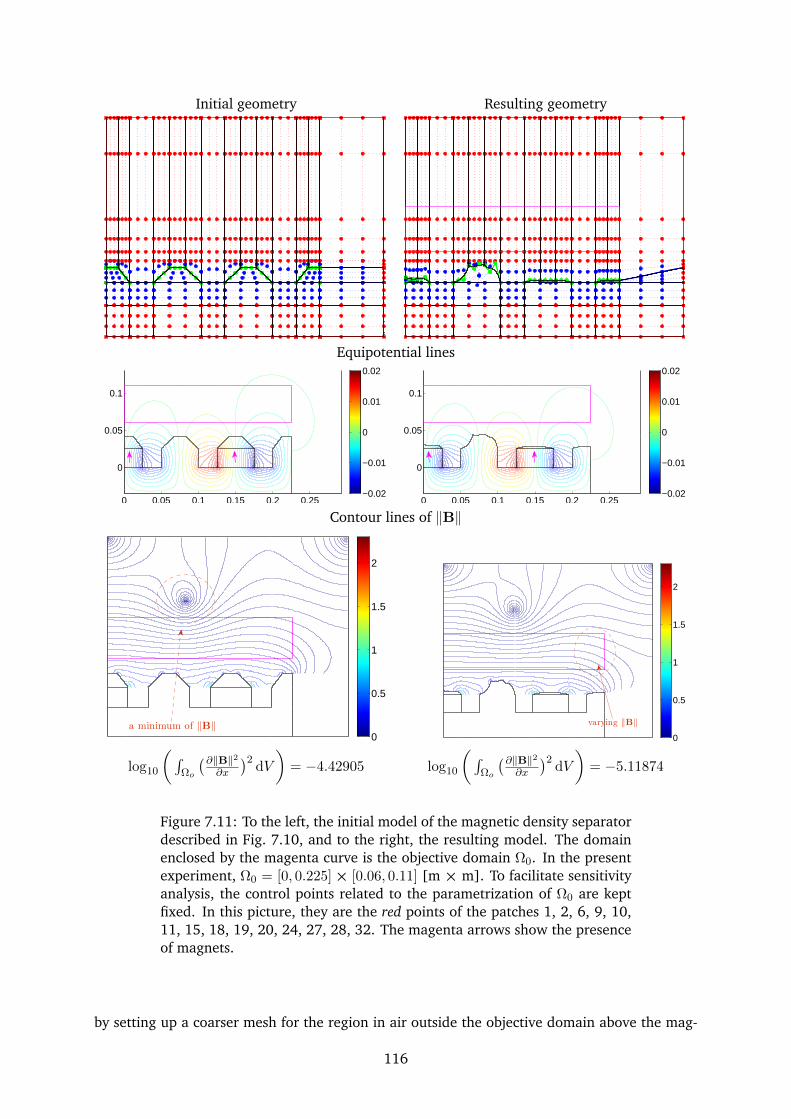
Initial geometry Resulting geometry
Equipotential lines
0 0.05 0.1 0.15 0.2 0.25
0
0.05
0.1
−0.02
−0.01
0
0.01
0.02
0 0.05 0.1 0.15 0.2 0.25
0
0.05
0.1
−0.02
−0.01
0
0.01
0.02
Contour lines of ‖B‖
0
0.5
1
1.5
2
a minimum of ‖B‖
0
0.5
1
1.5
2
varying ‖B‖
log10
(∫Ωo
(∂‖B‖2∂x
)2dV
)= −4.42905 log10
(∫Ωo
(∂‖B‖2∂x
)2dV
)= −5.11874
Figure 7.11: To the left, the initial model of the magnetic density separatordescribed in Fig. 7.10, and to the right, the resulting model. The domainenclosed by the magenta curve is the objective domain Ω0. In the presentexperiment, Ω0 = [0, 0.225]× [0.06, 0.11] [m × m]. To facilitate sensitivityanalysis, the control points related to the parametrization of Ω0 are keptfixed. In this picture, they are the red points of the patches 1, 2, 6, 9, 10,11, 15, 18, 19, 20, 24, 27, 28, 32. The magenta arrows show the presenceof magnets.
by setting up a coarser mesh for the region in air outside the objective domain above the mag-
116
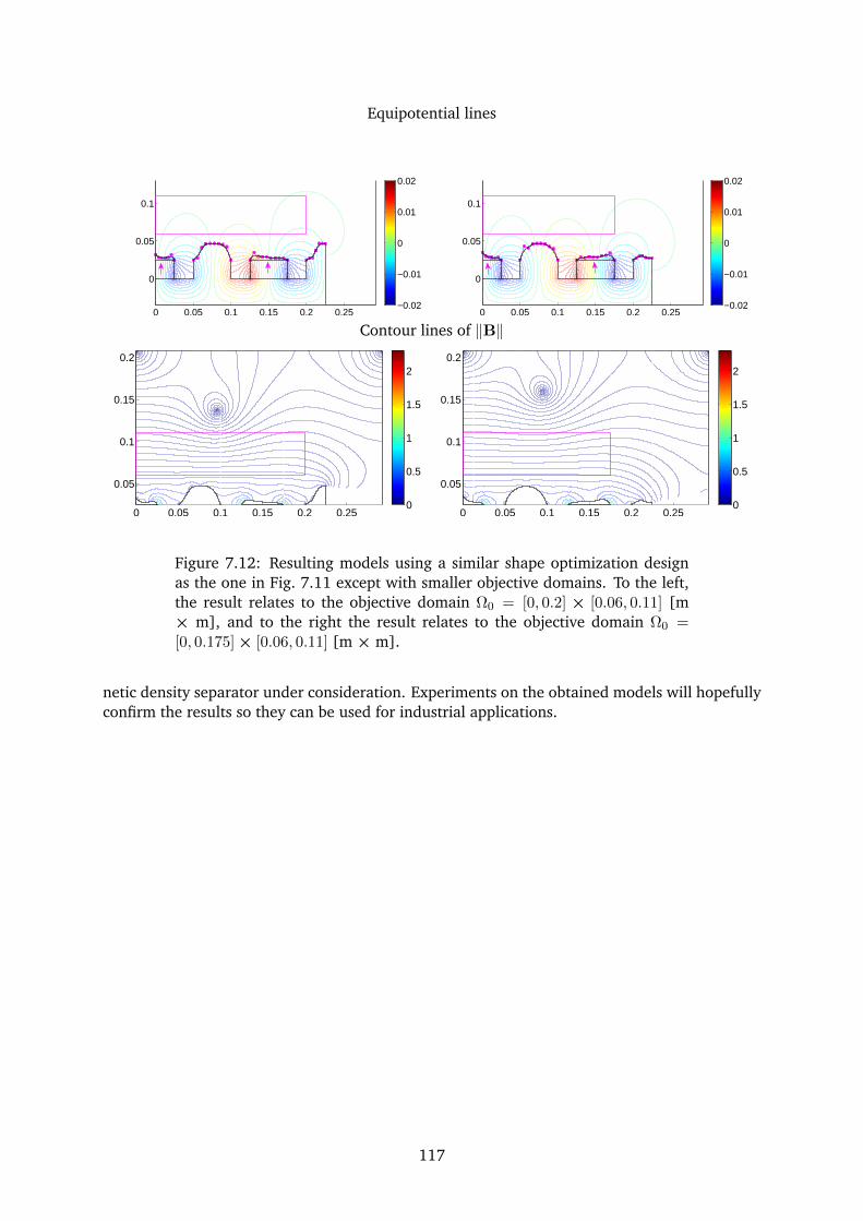
Equipotential lines
0 0.05 0.1 0.15 0.2 0.25
0
0.05
0.1
−0.02
−0.01
0
0.01
0.02
0 0.05 0.1 0.15 0.2 0.25
0
0.05
0.1
−0.02
−0.01
0
0.01
0.02
Contour lines of ‖B‖
0 0.05 0.1 0.15 0.2 0.25
0.05
0.1
0.15
0.2
0
0.5
1
1.5
2
0 0.05 0.1 0.15 0.2 0.25
0.05
0.1
0.15
0.2
0
0.5
1
1.5
2
Figure 7.12: Resulting models using a similar shape optimization designas the one in Fig. 7.11 except with smaller objective domains. To the left,the result relates to the objective domain Ω0 = [0, 0.2] × [0.06, 0.11] [m× m], and to the right the result relates to the objective domain Ω0 =[0, 0.175]× [0.06, 0.11] [m × m].
netic density separator under consideration. Experiments on the obtained models will hopefullyconfirm the results so they can be used for industrial applications.
117
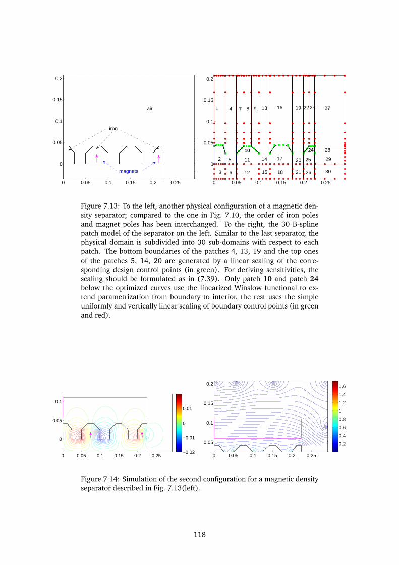
0 0.05 0.1 0.15 0.2 0.25
0
0.05
0.1
0.15
0.2
iron
magnets
air
0 0.05 0.1 0.15 0.2 0.25
0
0.05
0.1
0.15
0.2
1
30
29
28
27
26
25
24
2322
21
20
19
18
17
16
15
14
13
12
11
10
987
6
5
4
2
3
Figure 7.13: To the left, another physical configuration of a magnetic den-sity separator; compared to the one in Fig. 7.10, the order of iron polesand magnet poles has been interchanged. To the right, the 30 B-splinepatch model of the separator on the left. Similar to the last separator, thephysical domain is subdivided into 30 sub-domains with respect to eachpatch. The bottom boundaries of the patches 4, 13, 19 and the top onesof the patches 5, 14, 20 are generated by a linear scaling of the corre-sponding design control points (in green). For deriving sensitivities, thescaling should be formulated as in (7.39). Only patch 10 and patch 24below the optimized curves use the linearized Winslow functional to ex-tend parametrization from boundary to interior, the rest uses the simpleuniformly and vertically linear scaling of boundary control points (in greenand red).
0 0.05 0.1 0.15 0.2 0.25
0
0.05
0.1
−0.02
−0.01
0
0.01
0 0.05 0.1 0.15 0.2 0.25
0.05
0.1
0.15
0.2
0.2
0.4
0.6
0.8
1
1.2
1.4
1.6
Figure 7.14: Simulation of the second configuration for a magnetic densityseparator described in Fig. 7.13(left).
118
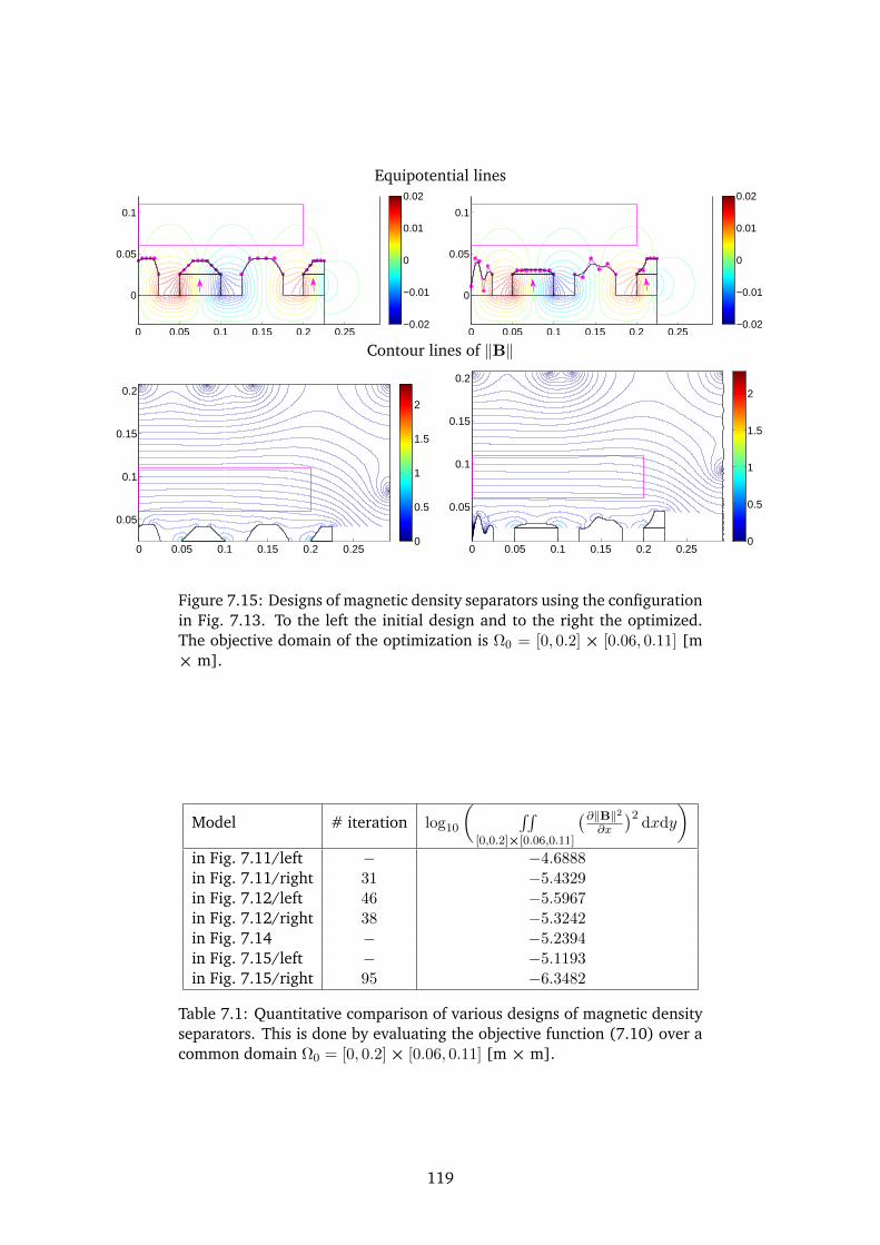
Equipotential lines
0 0.05 0.1 0.15 0.2 0.25
0
0.05
0.1
−0.02
−0.01
0
0.01
0.02
0 0.05 0.1 0.15 0.2 0.25
0
0.05
0.1
−0.02
−0.01
0
0.01
0.02
Contour lines of ‖B‖
0 0.05 0.1 0.15 0.2 0.25
0.05
0.1
0.15
0.2
0
0.5
1
1.5
2
0 0.05 0.1 0.15 0.2 0.25
0.05
0.1
0.15
0.2
0
0.5
1
1.5
2
Figure 7.15: Designs of magnetic density separators using the configurationin Fig. 7.13. To the left the initial design and to the right the optimized.The objective domain of the optimization is Ω0 = [0, 0.2]× [0.06, 0.11] [m× m].
Model # iteration log10
( ∫∫[0,0.2]×[0.06,0.11]
(∂‖B‖2∂x
)2dxdy
)
in Fig. 7.11/left − −4.6888in Fig. 7.11/right 31 −5.4329in Fig. 7.12/left 46 −5.5967in Fig. 7.12/right 38 −5.3242in Fig. 7.14 − −5.2394in Fig. 7.15/left − −5.1193in Fig. 7.15/right 95 −6.3482
Table 7.1: Quantitative comparison of various designs of magnetic densityseparators. This is done by evaluating the objective function (7.10) over acommon domain Ω0 = [0, 0.2]× [0.06, 0.11] [m × m].
119
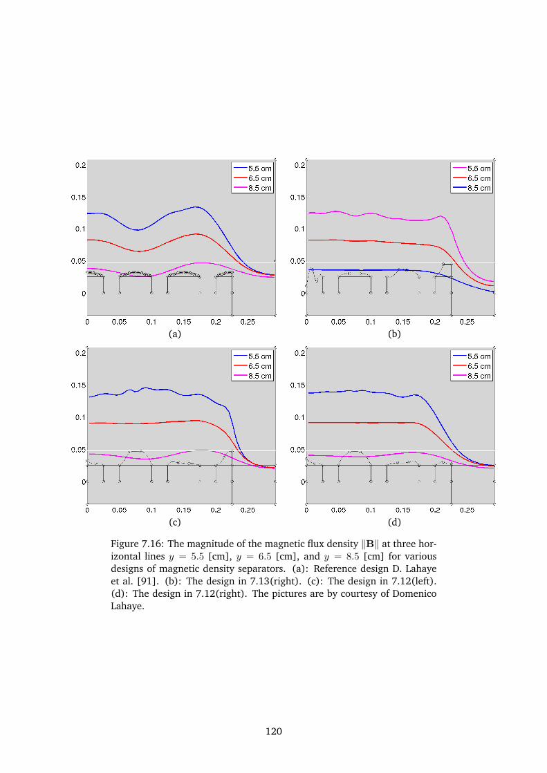
(a) (b)
(c) (d)
Figure 7.16: The magnitude of the magnetic flux density ‖B‖ at three hor-izontal lines y = 5.5 [cm], y = 6.5 [cm], and y = 8.5 [cm] for variousdesigns of magnetic density separators. (a): Reference design D. Lahayeet al. [91]. (b): The design in 7.13(right). (c): The design in 7.12(left).(d): The design in 7.12(right). The pictures are by courtesy of DomenicoLahaye.
120
Conclusions and future work
In this thesis, we have investigated the utilization of isogeometric analysis for shape optimizationfor several two dimensional electromagnetic problems. Within the problems, we have observedthat, when unphysical restrictions on the variation of the shape under consideration are avoidedas much as possible, a resulting design often outperforms an existing design. Thus they areworth considering for real engineering applications. Inspired by this observation:
• The resulting nano-antennas presented in Chapter 6 are being built and experimented.This is done by Sergey I. Bozhevolnyi, Morten Willatzen and their research group at Uni-versity of Southern Denmark.
• The resulting magnetic density separators presented in Chapter 7 are potentially built andexperimentally measured by Domenico Lahaye and his research group at Delft Universityof Technology.
Further potential future work are
1. Utilization of a local refinement method: It is important in many parts of the work pre-sented in this thesis to call in the utilization of a local refinement method. First, in theminimization problem of the Winslow functional presented in Fig. 2.1, each time there isa need to refine a knot interval tensor product [ui, ui+1]× [vj , vj+1], the present code willinsert a new knot to each dimension and the insertion will effect all other knot interval.Thus a local refinement method would certainly improve the computational efficiency ofthe code. Moreover, for the design problem of antennas discussed in Part III, in particular,when the size of the antennas are equivalent to several wavelength, it is very computa-tional beneficial or even necessary to use a local refinement along the interfaces of theantennas to capture the skindepth. Also in the space where the magnetic energy is con-centrated. Finally, for the design of magnetic density separators described in Part IV, alocal refinement is also important to save computational efficiency for a relatively large airregion above the objective domain.
2. Three-dimensional shape optimization of nano-antennas for field enhancement: It has beenpointed out in Fig. 6.10 that the 2D assumption for the design problem of nano-antennaspresented in Chapter 6 is insufficient for designing realistic 3D nano-antennas. Due tothe importance of such nano-antennas in nano-applications [81], it is very meaningfulfor investigating shape optimization of 3D nano-antennas. It may suffice to consider acylindrical antenna and perform shape optimization on its 2D cross-section while solvingthe numerical solution in 3D. Again, as the size of the antenna may be equivalent to severalwavelengths, a local refinement method is very important to save computational efficiencywhen dealing with 3D analysis.
3. Utilization of the manifold mapping method [99, 100, 101]: In the shape optimization prob-lem of antennas in Part III, we have observed that the optimal shape with respect to a meshand that with respect to a finer mesh are remarkably different, c.f. Fig. 5.14. Especially, ananalysis with very fine mesh and basis functions of high order is required to gain sufficient
121

accuracy for the numerical solution with respect to an optimal shape, c.f. Fig. 6.8. Thusit is too computational expensive to use such an analysis to calculate numerical values ina complete optimization process. Meanwhile, the manifold mapping method is capable offinding the optimum with respect to a finer mesh while mostly using the computationaleffort in evaluating numerical values with respect to a coarser mesh. Therefore, the uti-lization of the manifold method, also with possibly a combination with a local refinementmethod, for the shape optimization problem of antennas is worth investigating.
122
References
[1] T.J.R. Hughes, J.A. Cottrell, and Y. Bazilevs. Isogeometric analysis: CAD, finite elements,NURBS, exact geometry and mesh refinement. Comput. Methods Appl. Mech. Engrg.,194(39-41):4135–4195, 2005.
[2] O.C. Zienkiewicz and R.L. Taylor. The finite element method. Vol. 1. The basis. Butterworth-Heinemann, Oxford, fifth edition, 2000.
[3] J.A. Cottrell, A. Reali, Y. Bazilevs, and T.J.R. Hughes. Isogeometric analysis of structuralvibrations. Comput. Methods Appl. Mech. Engrg., 195(41-43):5257–5296, 2006.
[4] Y. Bazilevs, L. Beirao da Veiga, J.A. Cottrell, T.J.R. Hughes, and G. Sangalli. Isogeometricanalysis: approximation, stability and error estimates for h-refined meshes. Math. ModelsMethods Appl. Sci., 16(7):1031–1090, 2006.
[5] T.J.R. Hughes, A. Reali, and G. Sangalli. Duality and unified analysis of discrete ap-proximations in structural dynamics and wave propagation: comparison of p-methodfinite elements with k-method NURBS. Comput. Methods Appl. Mech. Engrg., 197(49-50):4104–4124, 2008.
[6] T.J.R. Hughes, J.A. Cottrell, and Y. Bazilevs. Isogeometric analysis: CAD, finite elements,NURBS, exact geometry and mesh refinement. Comput. Methods Appl. Mech. Engrg.,194(39-41):4135–4195, 2005.
[7] Yuri Bazilevs J.A. Cottrell, T.J.R. Hughes. Isogeometric Analysis: Toward Integration ofCAD and FEA. J. Wiley., West Sussex, 2009.
[8] Les Piegl and Wayne Tiller. The NURBS book. Monographs in Visual Communication.Berlin: Springer-Verlag. xiv, 646 p. DM 129.00; oS 941.70; sFr 124.00 , 1995.
[9] D.M. Nguyen, A. Evgrafov, A.R. Gersborg, and J. Gravesen. Isogeometric shape optimiza-tion of vibrating membranes. Computer Methods in Applied Mechanics and Engineering,200(13-16):1343 – 1353, 2011.
[10] D.M. Nguyen, A. Evgrafov, and J. Gravesen. Shape optimization of sub-wavelength an-tennas using isogeometric analysis. International Journal for numerical methods in engi-neering, submitted, 2011.
[11] W.A. Wall, M.A. Frenzel, and C. Cyron. Isogeometric structural shape optimization. Com-put. Methods Appl. Mech. Engrg., 197(33-40):2976–2988, 2008.
[12] Seonho Cho and Seung-Hyun Ha. Isogeometric shape design optimization: exact geom-etry and enhanced sensitivity. Struct. Multidiscip. Optim., 38(1):53–70, 2009.
[13] Xiaoping Qian. Full analytical sensitivities in nurbs based isogeometric shape optimiza-tion. Computer Methods in Applied Mechanics and Engineering, 199(29-32):2059 – 2071,2010.
123
[14] A.P. Nagy, M.M. Abdalla, and Z. Gurdal. Isogeometric sizing and shape optimisation ofbeam structures. Comput. Methods Appl. Mech. Engrg., 199(17-20):1216–1230, 2010.
[15] Attila P. Nagy, Mostafa M. Abdalla, and Zafer Gurdal. Isogeometric design of elasticarches for maximum fundamental frequency. Structural and Multidisciplinary Optimiza-tion, 43(1):135–149, 2011.
[16] Xiaoping Qian and Ole Sigmund. Isogeometric shape optimization of photonic crystalsvia Coons patches. Computer Methods in Applied Mechanics and Engineering, 200(25-28):2237–2255, 2011.
[17] Y. Ding. Shape optimization of structures: a literature survey. Computers & Structures,24(6):985 – 1004, 1986.
[18] Seonho Cho and Seung-Hyun Ha. Isogeometric shape design optimization: exact geom-etry and enhanced sensitivity. Struct. Multidiscip. Optim., 38(1):53–70, 2009.
[19] N.L. Pedersen. Optimization of holes in plates for control of eigenfrequencies. Struct.Multidiscip. Optim., 28(1):1–10, AUG 2004.
[20] N.L. Pedersen. On simultaneous shape and orientational design for eigenfrequency opti-mization. Struct. Multidiscip. Optim., 33(4-5):387–399, APR 2007.
[21] V. Braibant and C. Fleury. Shape optimal design using B-splines. Comput. Methods Appl.Mech. Engrg., 44(3):247 – 267, 1984.
[22] Jens Gravesen. Differential Geometry and Design of Shape and Motion. Department ofMathematics, Technical University of Denmark, 2002.
[23] Hartmut Prautzsch, Wolfgang Boehm, and Marco Paluszny. Bezier and B-spline techniques.Mathematics and Visualization. Springer-Verlag, Berlin, 2002.
[24] Les Piegl and Wayne Tiller. The NURBS book. Monographs in Visual Communication.Berlin: Springer-Verlag. xiv, 646 p. DM 129.00; oS 941.70; sFr 124.00 , 1995.
[25] Milton Abramowitz and Irene A. Stegun. Handbook of Mathematical Functions with For-mulas, Graphs, and Mathematical Tables. Dover, New York, 1964.
[26] R.A. Adams. Sobolev spaces. Pure and Applied Mathematics, Vol. 65. Academic Press, NewYork-London, 1975.
[27] R. D. Cook, D. S. Malkus, M. E. Plesha, and R. J. Witt. Concepts and applications of finiteelement analysis. John Wiley and Sons. Inc., fourth edition, 2002.
[28] J. Gravesen, A. Evgrafov, A.R. Gersborg, D.M. Nguyen, and P.N. Nielsen. Isogeometricanalysis and shape optimisation. Proceedings of NSCM-23: the 23rd Nordic Seminar onComputational Mechanics, 23:14–17, 2010.
[29] J. Gravesen, A. Evgrafov, and D. M. Nguyen. Parametrisation in 2-dimensional isogeo-metric analysis. in preparation.
[30] D.M. Nguyen, A. Evgrafov, A.R. Gersborg, and J. Gravesen. Isogeometric shape optimiza-tion of vibrating membranes. Computer Methods in Applied Mechanics and Engineering,200(13-16):1343 – 1353, 2011.
[31] P. Knupp and S. Steinberg. Fundamentals of Grid Generation. CRC Press, Boca Ranton,1993.
124
[32] L.V. Ahlfors. Complex analysis. An introduction to the theory of analytic functions of onecomplex variable, International Series in Pure and Applied Mathematics. McGraw-Hill BookCo., New York, third edition, 1978.
[33] MathWorks Inc.
[34] M.C. Delfour and J.P. Zolesio. Shapes and geometries. Analysis, differential calculus, andoptimization, volume 4 of Advances in Design and Control. Society for Industrial andApplied Mathematics (SIAM), Philadelphia, PA, 2001.
[35] B. Mohammadi and O. Pironneau. Applied Shape Optimization for Fluids. Oxford Univer-sity Press, 2001.
[36] Gregoire Allaire. Shape optimization by the homogenization method, volume 146 of Ap-plied Mathematical Sciences. Springer-Verlag, New York, 2002.
[37] M.P. Bendsøe and O. Sigmund. Topology optimization. Theory, methods and applications.Springer-Verlag, Berlin, 2003.
[38] J.A. Sethian. Level Set Methods and Fast Marching Methods : Evolving Interfaces in Com-putational Geometry, Fluid Mechanics, Computer Vision, and Materials Science. CambridgeUniversity Press, 1999.
[39] J.A. Cottrell, A. Reali, Y. Bazilevs, and T.J.R. Hughes. Isogeometric analysis of structuralvibrations. Comput. Methods Appl. Mech. Engrg., 195(41-43):5257–5296, 2006.
[40] Y. Bazilevs, L. Beirao da Veiga, J.A. Cottrell, T.J.R. Hughes, and G. Sangalli. Isogeometricanalysis: approximation, stability and error estimates for h-refined meshes. Math. ModelsMethods Appl. Sci., 16(7):1031–1090, 2006.
[41] T.J.R. Hughes, A. Reali, and G. Sangalli. Duality and unified analysis of discrete ap-proximations in structural dynamics and wave propagation: comparison of p-methodfinite elements with k-method NURBS. Comput. Methods Appl. Mech. Engrg., 197(49-50):4104–4124, 2008.
[42] A.P. Nagy, M.M. Abdalla, and Z. Gurdal. Isogeometric sizing and shape optimisation ofbeam structures. Comput. Methods Appl. Mech. Engrg., 199(17-20):1216–1230, 2010.
[43] Antoine Henrot. Minimization problems for eigenvalues of the Laplacian. J. Evol. Equ.,3(3):443–461, 2003.
[44] Zakaria Belhachmi, Dorin Bucur, Giuseppe Buttazzo, and Jean-Marc Sac-Epee. Shapeoptimization problems for eigenvalues of elliptic operators. ZAMM Z. Angew. Math. Mech.,86(3):171–184, 2006.
[45] Zhixue Wu. Optimal hole shape for minimum stress concentration using parameterizedgeometry models. Struct. Multidiscip. Optim., 37(6):625–634, FEB 2009.
[46] J.W. Hutchinson and F.I. Niordson. Designing vibrating membranes. In Continuummechanics and related problems of analysis (Russian), pages 581–590. Izdat. “Nauka”,Moscow, 1972.
[47] S.A. Wolf and J.B. Keller. Range of the first two eigenvalues of the laplacian. Proceedings:Mathematical and Physical Sciences, 447(1930):397–412, 1994.
[48] Dorin Bucur. Do optimal shapes exist? Milan J. Math., 75:379–398, 2007.
125
[49] Couro Kane and Marc Schoenauer. A drum shape optimisation by genetic algorithms.Complexity International, 2, 1995.
[50] L.E. Kinsler, A.R. Frey, A.B. Coppens, and J.V. Sanders. Fundamentals of Acoustics. JohnWiley & Sons, Singapore, 1982.
[51] D.R. Lapp. The Physics of Music and Musical Instruments. Wright Center for InnovativeScience Education, Tufts University, Medford, Massachusetts, 2003.
[52] C. de Boor and G.J. Fix. Spline approximation by quasiinterpolants. J. ApproximationTheory, 8:19–45, 1973.
[53] C. Gordon, D.L. Webb, and S. Wolpert. One cannot hear the shape of a drum. Bull. Amer.Math. Soc. (N.S.), 27(1):134–138, 1992.
[54] Jens Gravesen, Anton Evgrafov, and Nguyen Dang Manh. On the sensitivities of multipleeigenvalues. Structural and Multidisciplinary Optimization, 44(4):583–587, 2011.
[55] A.P. Seyranian, E. Lund, and N. Olhoff. Multiple eigenvalues in structural optimizationproblems. Structural Optimization, 8:207–227, 1994.
[56] N.L. Pedersen and A.K. Nielsen. Optimization of practical trusses with constraints oneigenfrequencies, displacements, stresses, and buckling. Struct. Multidiscip. Optim., 25(5-6):436–445, DEC 2003.
[57] J.S. Jensen and N.L. Pedersen. On maximal eigenfrequency separation in two-materialstructures: the 1D and 2D scalar cases. J. of Sound and Vibration, 289(4-5):967–986,FEB 7 2006.
[58] Jianbin Du and Niels Olhoff. Topological design of freely vibrating continuum structuresfor maximum values of simple and multiple eigenfrequencies and frequency gaps. Struct.Multidiscip. Optim., 34(2):91–110, AUG 2007.
[59] A. Buffa, G. Sangalli, and R. Vazquez. Isogeometric analysis in electromagnetics: B-splines approximation. Comput. Methods Appl. Mech. Engrg., 199(17-20):1143–1152,2010.
[60] M.P. Bendsøe and O. Sigmund. Topology optimization. Theory, methods and applications.Springer-Verlag, Berlin, 2003.
[61] Tosio Kato. Perturbation for Linear Operators. Springer, Germany, 1995.
[62] F. van Keulen, R.T. Haftka, and N.H. Kim. Review of options for structural design sen-sitivity analysis. part 1: Linear systems. Computer Methods in Applied Mechanics andEngineering, 194:3213–3243, 2005.
[63] A.P. Seyranian, E. Lund, and N. Olhoff. Multiple eigenvalues in structural optimizationproblems. Structural Optimization, 8:207–227, 1994.
[64] Andre Kurs, Aristeidis Karalis, Robert Moffatt, J. D. Joannopoulos, Peter Fisher, and MarinSoljacic. Wireless power transfer via strongly coupled magnetic resonances. Science,317(5834):83–86, 2007.
[65] Aristeidis Karalis, J. D. Joannopoulos, and Marin Soljacic. Efficient wireless non-radiativemid-range energy transfer. Annals of Physics, 323(1):34–48, 2008.
[66] Witricity corp.
126
[67] Bombardier corp.
[68] Leixiang Bian, Yumei Wen, Ping Li, Qiuling Gao, and Min Zheng. Magnetoelectric trans-ducer with high quality factor for wireless power receiving. Sensors and Actuators A:Physical, 150(2):207 – 211, 2009.
[69] B.L. Cannon, J.F. Hoburg, D.D. Stancil, and S.C. Goldstein. Magnetic resonant couplingas a potential means for wireless power transfer to multiple small receivers. Power Elec-tronics, IEEE Transactions on, 24(7):1819 –1825, july 2009.
[70] J. Choi and C. Seo. High-efficiency wireless energy transmission using magnetic reso-nance based on metamaterial with relative permeability equal to -1. Progress in electro-magnetics research-pier, 106:33–47, 2010.
[71] N. Aage, N.A. Mortensen, and O. Sigmund. Topology optimization of metallic devicesfor microwave applications. International Journal for numerical methods in engineering,83(2):228–248, 2010.
[72] L. Peng, O. Breinbjerg, and N.A. Mortensen. Wireless energy transfer through non-resonant magnetic coupling. Journal of Electromagnetic Waves and Applications, 24:1587–1598(12), July 2010.
[73] Aycan Erentok and Ole Sigmund. Topology Optimization of Sub-Wavelength Antennas.IEEE transactions on antennas and propagation, 59(1):58–69, 2011.
[74] N. Olhoff, M. P. Bendsøe, and J. Rasmussen. CAD-integrated structural topology anddesign optimization. In Shape and layout optimization of structural systems and optimalitycriteria methods, volume 325 of CISM Courses and Lectures, pages 171–197. Springer,Vienna, 1992.
[75] Yu-Deok Seo, Hyun-Jung Kim, and Sung-Kie Youn. Shape optimization and its extensionto topological design based on isogeometric analysis. International Journal of Solids andStructures, 47(11-12):1618 – 1640, 2010.
[76] G. Allaire. Conception optimale de structures, volume 58 of Mathematiques et Applications.Springer, 2007.
[77] Jianming Jin. The finite element method in electromagnetics. John Wiley & Sons, NewYork, 2002.
[78] Constantine A. Balanis. Advanced engineering electromagnetics. Wiley, New York, 2005.
[79] David K. Cheng. Fundamentals of engineering electromagnetics. Addison-Wesley, Reading,Massachusetts, 1993.
[80] N. Aage. Personal communication, 2011.
[81] G. Della Valle, T. Søndergaard, and S. I. Bozhevolnyi. High-q plasmonic resonators basedon metal split nanocylinders. Phys. Rev. B, 80:235405, 2009.
[82] Seungchul Kim, Jonghan Jin, Young-Jin Kim, In-Yong Park, Yunseok Kim, and Seung-Woo Kim. High-harmonic generation by resonant plasmon field enhancement. Nature,453:757–760, 2008.
[83] Daniel R. Ward, Falco Huser, Fabian Pauly, and Douglas Cuevas, Juan Carlos Natelson.Optical rectification and field enhancement in a plasmonic nanogap. Nat Nature, 5:732–736, 2010.
127
[84] Alexandre Aubry, Dang Yuan Lei, Antonio I. Fernandez-Domnguez, Yannick Sonnefraud,Stefan A. Maier, and J. B. Pendry. Plasmonic light-harvesting devices over the wholevisible spectrum. Nano Letters, 10(7):2574–2579, 2010.
[85] Alexandre Vial, Anne-Sophie Grimault, Demetrio Macıas, Dominique Barchiesi, andMarc Lamy de la Chapelle. Improved analytical fit of gold dispersion: application tothe modeling of extinction spectra with a finite-difference time-domain method. Phys.Rev. B, 71, 2005.
[86] COMSOL Inc.
[87] F. Di Maio, P. Rem, S. Serranti, and G. Bonifazi. The W2Plastics Project: Exploring theLimits of Polymer Separation. The Open Waste Management Journal, 3:90–98, 2010.
[88] V. Murariu, J. Svoboda, and P. Sergeant. The modelling of the separation process in aferrohydrostatic separator. Minerals Engineering, 18(4):449–457, 2005.
[89] V. Murariu and J. Svoboda. The effect of magnetic susceptibility on the motion of particlesin a ferrohydrostatic separator. Magnetic and Electrical Separation, 11:51–61, 2002.
[90] E. J. Bakker, P. C. Rem, and N. Fraunholcz. Upgrading mixed polyolefin waste withmagnetic density separation. Waste Management, 29(5):1712–1717, 2009.
[91] D. Lahaye, H. Polinder, and P. Rem. Magnet designs for magnetic density separation ofpolymers. The Journal of Solid Waste Technology and Management, 26:977–983, 2011.
[92] F. Weijmans, E. Bakker, and P.C. Rem. Magnetic density separation of diamonds fromgangue. Environmental Engineering and Management Journal, 8(4):981–984, 2009.
[93] L. Muchova and P. Rem. Precious metals in municipal solid waste incineration bottomash. Magnetic density separation, 39(9):107–116, 2009.
[94] J.R.A. de Koning, E.J. Bakker, and P. Rem. Sorting of vegetable seeds by magnetic densityseparation in comparison with liquid density separation. Seed Science and Technology ,39(3):593–603, 2011.
[95] B. Hu, F. Di Maio, P. Rem, G. Houzeaux, H. Calmet, and H. Owen. Development of inversemagnetic density separation of polyolefin mixtures. The Journal of Solid Waste Technologyand Management, 26:968–976, 2011.
[96] S. Serranti, A. Gargiulo, and G. Bonifazi. The use of hyperSpectral imaging for qualitycontrol in the MDS-based recycling process of polyolefins. The Journal of Solid WasteTechnology and Management, 26:952–967, 2011.
[97] P. P. Sylvester and R. L. Ferrari. Finite Elements for Electrical Engineers. Cambridge Uni-versity Press, New York, third edition, 1996.
[98] Personal communication of Domenico Lahaye with Peter Rem and his group at the DelftUniversity of Technology, 2012 .
[99] D. Echeverria, D. Lahaye, L. Encica, E.A. Lomonova, P.W. Hemker, and A.J.A. Vanden-put. Manifold-mapping optimization applied to linear actuator design. Magnetics, IEEETransactions on, 42(4):1183 –1186, april 2006.
[100] D. Lahaye, A. Canova, G. Gruosso, and M. Repetto. Adaptive manifold-mapping us-ing multiquadric interpolation applied to linear actuator design. COMPEL-The Interna-tional Journal for Computation and Mathematics in Electrical and Electronic Engineering,26(2):225–235, 2007.
128

[101] Anders A. Larsen, Martin Bendsøe, Jesper Hattel, and Henrik Schmidt. Optimizationof friction stir welding using space mapping and manifold mapping-an initial study ofthermal aspects. Structural and Multidisciplinary Optimization, 38(3):289–299, 2009.
129


![Shape Error Analysis of Functional Surface Based on ... · Isogeometric analysis (IGA) [18] is a method aimed at avoiding the discretization errors by using the same basis for analysis](https://img.pdfslide.us/doc/110x75/5e7b6bd3d7c5e65f99083e7a/shape-error-analysis-of-functional-surface-based-on-isogeometric-analysis-iga.jpg)