Embed Size (px)
Citation preview
University of Uppsala
Master Thesis
Geometry of BV Quantization andMathai-Quillen Formalism
Author:Luigi Tizzano
Supervisor:Maxim Zabzine
1
Abstract. Mathai-Quillen (MQ) formalism is a prescription to con-struct a Gaussian shaped Thom form for a vector bundle. The aimof this master thesis is to formulate a new Thom form representativeusing geometrical aspects of Batalin-Vilkovisky (BV) quantization. Inthe first part of the work we review the BV and MQ formalisms bothin finite dimensional setting. Finally, to achieve our purpose, we willexploit the odd Fourier transform considering the MQ representativeas a function over the appropriate graded manifold.
Contents
Chapter 1. Introduction 4
Chapter 2. Super Linear Algebra 72.1. Super Vector Spaces 72.2. Superalgebras 92.3. Berezin Integration 132.4. Change of Coordinates 142.5. Gaussian Integration 17
Chapter 3. Supermanifolds 213.1. Presheaves and Sheaves 213.2. Integration Theory 24
Chapter 4. Graded Geometry 284.1. Graded Linear Algebra 284.2. Graded Manifolds 29
Chapter 5. Odd Fourier transform and BV-formalism 315.1. Odd Fourier Transform 315.2. Integration Theory 345.3. Algebraic Aspects of Integration 375.4. Geometry of BV Quantization 41
Chapter 6. The Mathai-Quillen Formalism 456.1. General Remarks on Topological Quantum Field Theories 456.2. Euler Class 476.3. Thom Class 496.4. Equivariant Cohomology 536.5. Universal Thom Class 556.6. Mathai-Quillen Representative of the Thom Class 57
Chapter 7. BV representative of the Thom Class 637.1. Geometry of T [1]E 637.2. Odd Fourier Transform Revisited 647.3. Analysis of the BV Representative 66
2

CONTENTS 3
Chapter 8. Conclusions 69
Bibliography 71
CHAPTER 1
Introduction
The Batalin-Vilkovisky (BV) formalism is widely regarded as themost powerful and general approach to the quantization of gauge the-ories. The physical novelty introduced by BV formalism is to makepossible the quantization of gauge theories that are difficult to quantizewith the Fadeev-Popov method. In particular, it offers a prescriptionto perform path integrals for these theories. In quantum field theorythe path integral is understood as some sort of integral over infinite di-mensional functional space. Up to now there is no suitable definition ofthe path integral and in practice all heuristic understanding of the pathintegral is done by mimicking the manipulations of finite dimensionalintegrals. Thus, a proper understanding of the formal algebraic manip-ulations with finite dimensional integrals is crucial for a better insightto the path integrals. Such formalism firstly appeared in the papersof Batalin and Vilkovisky [6, 7] while a clear geometric interpretationwas given by Schwarz in [11, 14]. This thesis will largely follow thespirit of [15] where the authors described some geometrical propertiesof BV formalism related to integration theory on supermanifolds. Onthe odd tangent bundle there is a canonical way to integrate a functionof top degree while to integrate over the odd cotangent bundle we al-ways have to pick a density. Although the odd cotangent bundle doesnot have a nice integration property, it is however interesting becauseof his algebraic property due to the BV structure on it.
Characteristic classes play an essential role in the study of global prop-erties of vector bundles. Consider a vector bundle over a certain basemanifold, we would like to relate differential forms on the total spaceto differential forms on the basis, to do that we would like to integrateover the fiber and this is what the Thom class allows us. Basically theThom class can be thought as a gaussian shaped differential form oftop degree which has indices in the vertical direction along the fiber.Mathai and Quillen [17] obtained an explicit construction of the Thomclass using Berezin integration, a technique widely used in physics lit-erature. The physical significance of this construction was first pointed
4
1. INTRODUCTION 5
out, in an important paper of Atiyah and Jeffrey [22]. They discoveredthat the path integrals of a topological field theory of the Witten type[25] are integral representations of Thom classes of vector bundles ininfinite dimensional spaces. In his classic work [18] Witten showed thata topological gauge theory can be constructed by twisting N = 2 su-persymmetric Yang-Mills theory. Correlation functions of the twistedtheory are non other than Donaldson invariants of four-manifolds andcertain quantities in the supersymmetric gauge theory considered aredetermined solely by the topology, eliminating the necessity of com-plicated integrals. In this way topological field theories are convenienttesting grounds for subtle non perturbative phenomena appearing inquantum field theory.
Understanding the dynamical properties of non-abelian gauge fieldsis a very difficult problem, probably one of the most important andchallenging problem in theoretical physics. Infact the Standard Modelof fundamental interactions is based on non-abelian quantum gaugefield theories. A coupling constant in such theories usually decreasesat high energies and blows up at low energies. Hence, it is easy andvalid to apply perturbation theory at high energies. However, as theenergy decreases the perturbation theory works worse and completelyfails to give any meaningful results at the energy scale called Λ. There-fore, to understand the Λ scale physics, such as confinement, hadronmass spectrum and the dynamics of low-energy interactions, we neednon-perturbative methods. The main such methods are based on su-persymmetry and duality. Like any symmetry, supersymmetry imposessome constraints on the dynamics of a physical system. Then, the dy-namics is restricted by the amount of supersymmetry imposed, but westill have a very non-trivial theory and thus interesting for theoreticalstudy. Duality means an existence of two different descriptions of thesame physical system. If the strong coupling limit at one side of theduality corresponds to the weak coupling limit at the other side, suchduality is especially useful to study the theory. Indeed, in that casedifficult computations in strongly coupled theory can be done pertur-batively using the dual weakly coupled theory.
The aim of this master thesis is to establish a relationship betweengeometrical aspects of BV quantization and the Mathai-Quillen for-malism for vector bundle. We will formulate a new representative ofthe Thom class, called BV representative. To reach this goal we will usethe odd Fourier transform as explained in [15]. However, we will gen-eralize this construction to the case of differential forms over a vector
1. INTRODUCTION 6
bundle. Lastly, we will show that our BV representative is authenti-cally a Thom class and that our procedure is consistent.
The outline of the thesis is as follows. In section 2 we discuss somebasic notions of super linear algebra. We pay particular attention tothe Berezinian integration in all its details, by giving detailed proofsof all our statements. In section 3 we treat the differential geometryof supermanifolds. As main examples we discuss the odd tangent andodd cotangent bundles. We also review the integration theory froma geometric point of view, following the approach of [1]. In section 4we briefly illustrate the Z-graded refinement of supergeometry, knownas graded geometry. In section 5 we define the odd Fourier transformwhich will be an object of paramount importance trough all the the-sis. Then, the BV structure on the odd cotangent bundle is introducedas well as a version of the Stokes theorem. Finally, we underline thealgebraic aspects of integration within BV formalism. In section 6 weexplain the Mathai-Quillen (MQ) formalism. Firstly, we describe topo-logical quantum field theories, then we introduce the notions of Thomclass and equivariant cohomology and eventually we give an explicitproof of the Poincare-Hopf theorem using the MQ representative. Insection 7 it is contained the original part of this work. Here, we discussour procedure to create a BV representative of the Thom class andobtain the desired relationship between BV quantization and Mathai-Quillen formalism. Section 8 is the conlusive section of this thesis wherewe summarize our results and discuss open issues.
CHAPTER 2
Super Linear Algebra
Our starting point will be the construction of linear algebra in thesuper context. This is an important task since we need these conceptsto understand super geometric objects. Super linear algebra deals withthe category of super vector spaces over a field k. In physics k is R orC. Much of the material described here can be found in books such as[2, 4, 5, 8, 12].
2.1. Super Vector Spaces
A super vector space V is a vector space defined over a field K witha Z2 grading. Usually in physics K is either R or C. V has the followingdecomposition
V = V0 ⊕ V1 (2.1)
the elements of V0 are called even and those of V1 odd. If di is thedimension of Vi we say that V has dimension d0|d1. Consider twosuper vector spaces V , W , the morphisms from V toW are linear mapsV → W that preserve gradings. They form a linear space denoted byHom(V,W ). For any super vector space the elements in V0 ∪ V1 arecalled homogeneous, and if they are nonzero, their parity is defined tobe 0 or 1 according as they are even or odd. The parity function isdenoted by p. In any formula defining a linear or multilinear objectin which the parity function appears, it is assumed that the elementsinvolved are homogeneous.If we take V = Kp+q with its standard basis ei with 1 ≤ i ≤ p + q ,and we define ei to be even if i ≤ p or odd if i > p, then V becomes asuper vector space with
V0 =p
i=1
Kei V1 =q
i=p+1
Kei (2.2)
then V will be denoted Kp|q.The tensor product of super vector spaces V and W is the tensor prod-uct of the underlying vector spaces, with the Z2 grading
(V ⊗W )k = ⊕i+j=k
Vi ⊗Wj (2.3)
7
2.1. SUPER VECTOR SPACES 8
where i, j, k are in Z2. Thus
(V ⊗W )0 = (V0 ⊗W0)⊕ (V1 ⊗W1)
(V ⊗W )1 = (V0 ⊗W1)⊕ (V1 ⊗W0)(2.4)
For super vector spaces V,W , the so called internal Hom , denoted byHom(V,W ), is the vector space of all linear maps from V to W . Inparticular we have the following definitions
Hom(V,W )0 = T : V → W |T preserves parity (= Hom(V,W ));
Hom(V,W )1 = T : V → W |T reverses parity
For example if we take V = W = K1|1 and we fix the standard basis,we have that
Hom(V,W ) =
a 00 d
|a, d ∈ K
;
Hom(V,W ) =
a bc d
|a, b, c, d ∈ K
(2.5)
If V is a super vector space, we write End(V ) for Hom(V, V ).
Example 2.1.1. Consider purely odd superspace ΠRq = R0|q overthe real number of dimension q. Let us pick up the basis θi, i =1, 2, ..., q and define the multiplication between the basis elements sat-isfying θiθj = −θjθi. The functions C∞(R0|q) on R0|q are given by thefollowing expression
f(θ1, θ2, ..., θq) =q
l=0
1
l!fi1i2...ilθ
i1θi2 ...θil (2.6)
and they correspond to the elements of exterior algebra ∧•(Rq)∗. Theexterior algebra
∧• (Rq)∗ = (∧even(Rq)∗)
∧
odd(Rq)∗
(2.7)
is a supervector space with the supercommutative multiplications givenby wedge product. The wedge product of the exterior algebra correspondsto the function multiplication in C∞(R0|q).
2.2. SUPERALGEBRAS 9
2.1.1. Rule of Signs. The ⊗ in the category of vector spaces isassociative and commutative in a natural sense. Thus, for ordinaryvector spaces U, V,W we have the natural associativity isomorphism
(U ⊗ V )⊗W U ⊗ (V ⊗W ), (u⊗ v)⊗ w −→ u⊗ (v ⊗ w) (2.8)
and the commutativity isomorphism
cV,W : V ⊗W W ⊗ V, v ⊗ w −→ w ⊗ v (2.9)
For the category of super vector spaces the associativity isomorphismremains the same, but the commutativity isomorphism is subject tothe following change
cV,W : V ⊗W W ⊗ V, v ⊗ w −→ (−1)p(v)p(w)w ⊗ v (2.10)
This definition is the source of the rule of signs, which says that when-ever two terms are interchanged in a formula a minus sign will appearif both terms are odd.
2.2. Superalgebras
In the ordinary setting, an algebra is a vector space A with a mul-tiplication which is bilinear. We may therefore think of it as a vectorspace A together with a linear map A⊗A → A, which is the multipli-cation. Let A be an algebra , K a field by which elements of A can bemultiplied. In this case A is called an algebra over K.Consider a set Σ ⊂ A, we will denote by A(Σ) a collection of all possiblepolynomials of elements of Σ. If f ∈ A(Σ) we have
f = f0 +
k≥1
i1,...,ik
fi1,...,ikai1 ...aik , ai ∈ Σ, fi1,...,ik ∈ K (2.11)
Of course A(Σ) is a subalgebra of A, called a subalgebra generated bythe set Σ. If A(Σ) = A, the set Σ is called a system of generators ofalgebra A or a generating set.
Definition 2.2.1. A superalgebra A is a super vector space A, givenwith a morphism , called the product: A ⊗ A → A. By definition ofmorphisms, the parity of the product of homogeneous elements of A isthe sum of parities of the factors.
The superalgebra A is associative if (xy)z = x(yz) ∀ x, y, z ∈ A. Aunit is an even element 1 such that 1x = x1 = x ∀x ∈ A. By now wewill refer to superalgebra as an associative superalgebra with the unit.
2.2. SUPERALGEBRAS 10
Example 2.2.2. If V is a super vector space, End(V ) is a superal-gebra. If V = Kp|q we write M(p|q) for End(V ). Using the standardbasis we have the usual matrix representations for elements of M(p|q)in the form
A BC D
(2.12)
where the letters A,B,C,D denotes matrices respectively of orders p×p, p × q, q × p, q × q and where the even elements the odd ones are,respectively, of the form.
A 00 D
,
0 BC 0
(2.13)
A superalgebra is said to be commutative if
xy = (−1)p(x)p(y)yx , ∀x, y ∈ A ; (2.14)
commutative superalgebra are often called supercommutative.
2.2.1. Supertrace. Let V = V0 ⊕ V1 a finite dimensional supervector space, and let X ∈ End(V ). Then we have
X =
X00 X01
X10 X11
(2.15)
where Xij is the linear map from Vj to Vi such that Xijv is the pro-jection onto Vi of Xv for v ∈ Vj. Now the supertrace of X is definedas
str(X) = tr(X00)− tr(X11) (2.16)
Let Y, Z be rectangular matrices with odd elements, we have the fol-lowing result
tr(Y Z) = −tr(ZY ) (2.17)
to prove this statement we denote by yik, zik the elements of matricesY and Z respectively then we have
tr(Y Z) =
yikzki = −
zkiyik = −tr(ZY ) (2.18)
notice that anologous identity is known for matrices with even elementsbut without the minus sign. Now we can claim that
str(XY ) = (−1)p(X)p(Y )str(Y X), X, Y ∈ End(V ) (2.19)
2.2. SUPERALGEBRAS 11
2.2.2. Berezinian. Consider a super vector space V , we can writea linear transformation of V in block form as
W =
A BC D
(2.20)
where here A and D are respectively p× p and q× q even blocks, whileB and C are odd. An explicit formula for the Berezinian is
Ber(W ) = det(A− BD−1C) det(D)−1 (2.21)
notice that the Berezinian is defined only for matrices W such that Dis invertible. As well as the ordinary determinant also the Berezinianenjoys the multiplicative property, so if we consider two linear trans-formations W1 and W2, like the ones that we introduced above , suchthat W = W1W2 we will have
Ber(W ) = Ber(W1)Ber(W2) (2.22)
To prove this statement firstly we define the matrices W1 and W2 toget
W1 =
A1 B1
C1 D1
, W2 =
A2 B2
C2 D2
=⇒ W =
A1A2 +B1C2 A1B2 +B1D2
C1A2 +D1C2 C1B2 +D1D2
(2.23)
Using matrix decomposition we can write for W1
W1 =
1 B1D
−11
0 1
A1 − B1D
−11 C1 0
0 D1
1 0
D−11 C1 1
= X+1 X
01X
−1
(2.24)
obviously this is true also for W2. So now we want to compute thefollowing Berezinian
Ber(W ) = Ber(X+1 X
01X
−1 X
+2 X
02X
−2 ) (2.25)
As a first step we consider two block matrices X and Y such that
X =
1 A0 1
, Y =
B CD E
(2.26)
we can see that X resembles the form of X+1 . Computing the Berezini-
ans we get
Ber(X)Ber(Y ) = det(B − CE−1D) det(E)−1 (2.27)
while
Ber(XY ) = det(B + AD − (C + AE)E−1D) det(E)−1 (2.28)
2.2. SUPERALGEBRAS 12
after this first check we can safely write that
Ber(W ) = Ber(X+1 )Ber(X
01X
−1 X
+2 X
02X
−2 ) (2.29)
As a second step we consider once again two block matrices X and Ynow defined as
X =
A 00 B
, Y =
C DE F
(2.30)
clearly now X resembles the form of X01 . Computing the Berezinians
we get
Ber(X)Ber(Y ) = det(A) det(B)−1 det(C −DF−1E) det(F )−1
= det(AC − ADF−1E) det(BF )−1(2.31)
while
Ber(XY ) = det(AC − ADF−1B−1BE) det(BF )−1 (2.32)
so after this second step we conlude that
Ber(W ) = Ber(X+1 )Ber(X
01 )Ber(X
−1 X
+2 X
02X
−2 ) (2.33)
Now repeating two times more the procedure done in the first two stepswe get the following result
Ber(W ) = Ber(X+1 )Ber(X
01 )Ber(X
−1 X
+2 )Ber(X
02 )Ber(X
−2 ) (2.34)
Now we want to show the multiplicativity of Ber(X−1 X
+2 ) but we can’t
proceed as in the previous steps. In fact if we consider once again twomatrices X and Y such that
X =
1 0C 1
, Y =
1 B0 1
(2.35)
we have thatBer(X)Ber(Y ) = 1
Ber(XY ) = det(1− B(1 + CB)−1C) det(1 + CB)−1 (2.36)
To guarantee the multiplicative property also in this case we have toprove that
det(1− B(1 + CB)−1C) det(1 + CB)−1 = 1 (2.37)
We may assume that B is an elementary matrix, which it means thatall but one entry of B are 0, and that one is an odd element b. By thisproperty we see that (CB)2 = 0, consequently
(1 + CB)−1 = 1− CB (2.38)
and hence
1− B(1 + CB)−1C = 1− B(1− CB)C = 1− BC (2.39)
2.3. BEREZIN INTEGRATION 13
Now we can use the general formula
det(1− BC) =∞
k=0
1
k!
∞
j=1
(−1)2j+1
jtr((BC)j)
k
= 1− tr(BC)
(2.40)Using the same formula we get the following result
det(1 + CB)−1 = (1 + tr(CB))−1 = (1− tr(BC))−1 (2.41)
where in the last passage we used (2.18). Eventually we can easilyverify that
det(1−B(1 + CB)−1C) det(1 + CB)−1
= (1− tr(BC))(1− tr(BC))−1 = 1(2.42)
At this point we may write
Ber(W ) = Ber(X+1 )Ber(X
01 )Ber(X
−1 )Ber(X
+2 )Ber(X
02 )Ber(X
−2 )
= Ber(X+1 X
01X
−1 )Ber(X
+2 X
02X
−2 )
= Ber(W1)Ber(W2)(2.43)
If we use another matrix decomposition for the matrix W defined in(2.20) we get an equivalent definition of the Berezinian which is
Ber(W ) = det(A) det(D − CA−1B)−1 (2.44)
2.3. Berezin Integration
Consider the super vector space Rp|q, it admits a set of generatorsΣ = (t1 . . . tp|θ1 . . . θq) with the properties
titj = tjti 1 ≤ i, j ≤ p (2.45)
θiθj = −θjθi 1 ≤ i, j ≤ q (2.46)
in particular (θi)2 = 0. We will referer to the (t1 . . . tp) as the even(bosonic)coordinates and to the (θ1 . . . θq) as the odd(fermionic) coordinates. OnRp|q, a general function g can be expanded as a polynomial in the θ’s:
g(t1 . . . tp|θ1 . . . θq) = g0(t1 . . . tp)+· · ·+θqθq−1 . . . θ1gq(t
1 . . . tp). (2.47)
The basic rules of Berezin integration are the following
dθ = 0
dθ θ = 1 (2.48)
2.4. CHANGE OF COORDINATES 14
by these rules, the integral of g is defined as
Rp|q[dt1 . . . dtp|dθ1 . . . dθq]g(t1 . . . tp|θ1 . . . θq) =
Rp
dt1 . . . dtpgq(t1 . . . tp)
(2.49)Since we require that the formula (2.49) remains true under a changeof coordinates, we need to obtain the transformation rule for the inte-gration form [dt1 . . . dtp|dθ1 . . . dθq]. In fact, although we know how thethings work in the ordinary(even) setting, we have to understand thebehavior of the odd variables in this process.
2.4. Change of Coordinates
Consider the simplest transformation for an odd variables
θ −→ θ = λθ, λ constant. (2.50)
then the equations (2.48) imply
dθ θ =
dθ θ = 1 ⇐⇒ dθ = λ−1dθ (2.51)
as we can see dθ is multiplied by λ−1, rather than by λ as one wouldexpect.Now we consider the case of Rq, where q denotes the number of oddvariables, and perform the transformation
θi −→ θi = f i(θ1 . . . θq) (2.52)
where f is a general function. Now we can expand f i in the followingmanner
f i(θ1 . . . θq) = θkf ik + θkθlθmf i
klm + . . . (2.53)
since the θi variables has to respect the anticommuting relation (2.46),the function f imust have only odd numbers of the θi variables in eachfactor. Now we compute the product
θq . . . θ1 = (θkqf qkq+ . . . )(θkq−1f q−1
kq−1+ . . . ) . . . . . . (θk1f 1
k1 + . . . )
= θkqθkq−1 . . . θk1f qkqf q−1kq−1
. . . f 1k1
= θqθq−1 . . . θ1εkq ...k1f qkqf q−1kq−1
. . . f 1k1
= θqθq−1 . . . θ1 det(F )
(2.54)
where in the last passage we used the usual formula for the determinantof the F matrix. We are ready to perform the Berezin integral in thenew variables θ
dθ1 . . . dθq θq . . . θ1 =
dθ1 . . . dθq θqθq−1 . . . θ1 det(F ) (2.55)
2.4. CHANGE OF COORDINATES 15
preserving the validity of (2.48) implies
dθ1 . . . dθq = det(F )−1dθ1 . . . dθq (2.56)
Using this result it is possible to define the transformation rule forBerezin integral under this transformation
t −→ t = t(t1 . . . tp)
θ −→ θ = θ(θ1 . . . θq)(2.57)
which is
Rp|q[dt1 . . . dtp|dθ1 . . . dθq]g(t1 . . . tp|θ1 . . . θq)
=
Rp|q[dt 1 . . . dtp|dθ 1 . . . dθq] det
∂t
∂t
det
∂θ
∂θ
−1
g(t 1 . . .tp|θ 1 . . . θq)
(2.58)
From this formula is clear that the odd variables transforms with theinverse of the Jacobian matrix determinant; the inverse of what happenin the ordinary case. At this point a question naturally arises: providedthat we are respecting the original parity of the variables, what doesit happen if the new variables undergo a mixed transformation ? Toanswer at this question we have to study a general change of coordinatesof the form
t −→ t = t(t1 . . . tp|θ1 . . . θq)
θ −→ θ = θ(t1 . . . tp|θ1 . . . θq)(2.59)
The Jacobian of this transformation will be a block matrix
W =
A BC D
=
1 0
CA−1 D
A 00 D−1
1 A−1B0 D − CA−1B
= W+W 0W−(2.60)
where A =∂t
∂tand D =
∂θ
∂θare the even blocks while B =
∂t
∂θand
C =∂θ
∂tare the odd ones. The matrix decomposition suggests that
we can think at the general change of coordinates as the product ofthree distinct transformations represented by the three block matricesin the right hand side of (2.60). At the moment we only know how todeal with a transformation of the type (2.57) which have a Jacobianmatrix like W 0. To proceed further we have to analyze the remaining

2.4. CHANGE OF COORDINATES 16
transformations
t −→ t = t(t1 . . . tp)
θ −→ θ = θ(t1 . . . tp|θ1 . . . θq)(2.61)
t −→ t = t(t1 . . . tp|θ1 . . . θq)
θ −→ θ = θ(θ1 . . . θq)(2.62)
Consider the case (2.61) then we rewrite the transformation as
t −→ t = h(t1 . . . tp)
θ −→ θ = g(t1 . . . tp|θ1 . . . θq)(2.63)
where f and g are general functions. By formula (2.49) we know how toperform the Berezin integration for a function F (t1 . . . | . . . θq). Usingthe new variables will give
[dt 1 . . . dt p|dθ1 . . . dθq]F (t 1 . . . | . . . θq)
=
[dt 1 . . . dt p|dθ1 . . . dθq]
F0(t 1 . . .t p)+ · · ·+θq . . . θ1 Fq(t 1 . . .t p)
(2.64)
where we used (2.47). As we did in (2.53) we expand g as
gi(t1 . . . | . . . θq) = θkqgikq(t1 . . . tp) + θkqθlqθmqgikqlqmq
(t1 . . . tp) + . . .(2.65)
and similary to (2.54) we get
θq . . . θ1 = θq . . . θ1 det[G(t1 . . . tp)] (2.66)
Inserting this result inside (2.64) we obtain[dt 1 . . . | . . . dθq]F (t 1 . . . | . . . θq) =
=
[dt 1 . . . | . . . dθq]
F0(t 1 . . .t p)+
· · ·+ θq . . . θ1 det[G(t1 . . . tp)] Fq(t 1 . . .t p)
(2.67)
as seen before if we want to achieve the same conclusion of (2.49) wedemand that
[dt 1 . . . | . . . dθq] = det[H(t1 . . . tp)] det[G(t1 . . . tp)]−1[dt1 . . . | . . . dθq](2.68)
The matrix W+ in equation (2.60) is the Jacobian of a change of coor-dinates which is a special case of the one that we studied in (2.63). In(2.68) we found that for this type of transformations, the integration
2.5. GAUSSIAN INTEGRATION 17
form behaves exaclty as in (2.58). A similiar argument can be usedfor transformations like (2.62) and consequently for W−. Finally, wediscovered the complete picture for the mixed change of coordinateswhich is
[dt 1 . . . | . . . dθq] = det(A) det(D − CA−1B)−1[dt1 . . . | . . . dθq]
= Ber(W )[dt1 . . . | . . . dθq](2.69)
where in the last passage we used the definition given in (2.44). Equa-tion (2.69) gives rise to the rule for the change of variables in Rp|q.In fact, if we express the integral of a function g(t1 . . . | . . . tp) definedon a coordinate system T = t1 . . . | . . . θq in a new coordinate systemT = t 1 . . . | . . . θq the relation is
[dt1 . . . | . . . dθq]g(t1 . . . | . . . θq)
=
Ber
∂T
∂ T
[dt 1 . . . | . . . dθq]g(t 1 . . . | . . . θq).
(2.70)
2.5. Gaussian Integration
Prior to define how to perform Gaussian integration with odd vari-ables we will recall some results using even variables. For example con-sider a p×p symmetric and real matrix A, then it is well known that wecan always find a matrix R ∈ SO(p) such that RAR = diag(λ1 . . .λp),where λi are the real eigenvalue of the matrix A. As a consequence weget
Z(A) =
dt1 . . . dtp exp
−
1
2tAt
=
dy1 . . . dyp exp
−
1
2(Ry)A(Ry)
=
dy1 . . . dyp exp
−
1
2
p
i=1
λi(yi)2
=p
i=1
+∞
−∞dyi exp
−
1
2λi(y
i)2
=p
i=1
2π
λi
12
= (2π)p2 (detA)−
12
(2.71)
Moreover if we consider the case of 2p integration variables xi andyi,i = 1 . . . p, and we assume that the integrand is invariant under
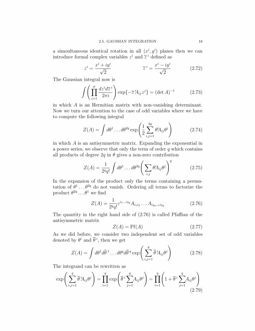
2.5. GAUSSIAN INTEGRATION 18
a simoultaneous identical rotation in all (xi, yi) planes then we canintroduce formal complex variables zi and z i defined as
zi =xi + iyi√2
z i =xi − iyi√2
(2.72)
The Gaussian integral now is
p
i=1
dzidz i
2πi
exp−z iAijz
j = (detA)−1 (2.73)
in which A is an Hermitian matrix with non-vanishing determinant.Now we turn our attention to the case of odd variables where we haveto compute the following integral
Z(A) =
dθ1 . . . dθ2q exp
1
2
2q
i,j=1
θiAijθj
(2.74)
in which A is an antisymmetric matrix. Expanding the exponential ina power series, we observe that only the term of order q which containsall products of degree 2q in θ gives a non-zero contribution
Z(A) =1
2qq!
dθ1 . . . dθ2q
i,j
θiAijθj
q
(2.75)
In the expansion of the product only the terms containing a permu-tation of θ1 . . . θ2q do not vanish. Ordering all terms to factorize theproduct θ2q . . . θ1 we find
Z(A) =1
2qq!εi1...i2qAi1i2 . . . Ai2q−1i2q (2.76)
The quantity in the right hand side of (2.76) is called Pfaffian of theantisymmetric matrix
Z(A) = Pf(A) (2.77)
As we did before, we consider two independent set of odd variablesdenoted by θi and θ i, then we get
Z(A) =
dθ1dθ 1 . . . dθqdθ q exp
q
i,j=1
θ iAijθj
(2.78)
The integrand can be rewritten as
exp
q
i,j=1
θ iAijθj
=
q
i=1
exp
θ i
q
j=1
Aijθj
=
q
i=1
1 + θ i
q
j=1
Aijθj
(2.79)

2.5. GAUSSIAN INTEGRATION 19
Expanding the product, we see that
Z(A) = εj1...jqAqjqAq−1jq−1 . . . A1j1 = det(A) (2.80)
which is,once again, the inverse of what happen in the ordinary case.As a final example in which the superdeterminant makes its appearancewe shall evaluate the Gaussian integral
Z(M) =
dt1 . . . | . . . dθq
exp
−
1
2
t1 . . . | . . . θq
M
t1...−
...θq
(2.81)here M is a block matrix of dimension (p, q) like
M =
A CC B
(2.82)
where A = A and B = −B are the even blocks and C the odd one.The first step is to carry out the change of coordinates
ti −→ t i = ti + A−1 ijCjkθk
θi −→ θ i = θi(2.83)
this is a transformation of (2.61) type with a unit Berezinian. Now theintegral takes the form
Z(M) =
dt 1 . . . | . . . dθ q
exp
−
1
2
t 1 . . . | . . . θ q
M
t 1...−
...θ q
(2.84)
where M has the diagonal block form
M =
A 00 B + CA−1C
(2.85)
We assume that the matrices A and B−CA−1C are nonsingular withA and B respectively symmetric and antisymmetric matrices. Thenthere exist real orthogonal matrices O1 and O2, of determinant +1,
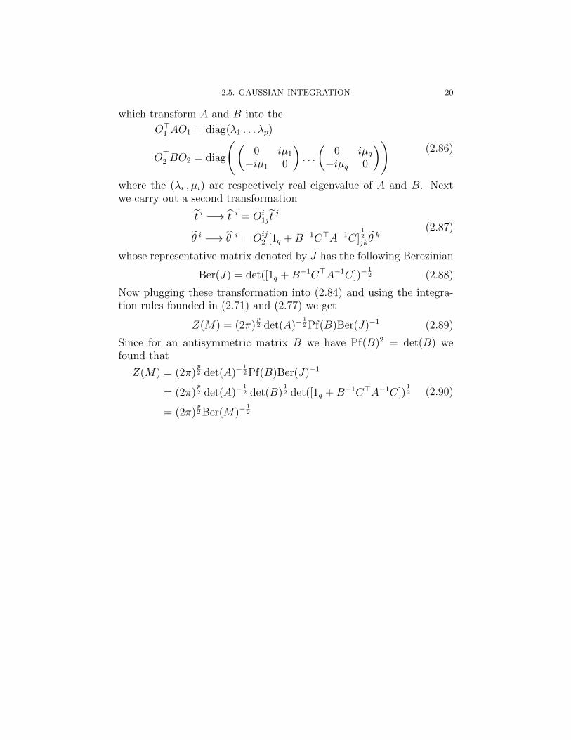
2.5. GAUSSIAN INTEGRATION 20
which transform A and B into the
O1 AO1 = diag(λ1 . . .λp)
O2 BO2 = diag
0 iµ1
−iµ1 0
. . .
0 iµq
−iµq 0
(2.86)
where the (λi , µi) are respectively real eigenvalue of A and B. Nextwe carry out a second transformation
t i −→ t i = Oi1jt j
θ i−→ θ i = Oij
2 [1q +B−1CA−1C]12jkθ k
(2.87)
whose representative matrix denoted by J has the following Berezinian
Ber(J) = det([1q +B−1CA−1C])−12 (2.88)
Now plugging these transformation into (2.84) and using the integra-tion rules founded in (2.71) and (2.77) we get
Z(M) = (2π)p2 det(A)−
12Pf(B)Ber(J)−1 (2.89)
Since for an antisymmetric matrix B we have Pf(B)2 = det(B) wefound that
Z(M) = (2π)p2 det(A)−
12Pf(B)Ber(J)−1
= (2π)p2 det(A)−
12 det(B)
12 det([1q +B−1CA−1C])
12
= (2π)p2Ber(M)−
12
(2.90)
CHAPTER 3
Supermanifolds
Roughly speaking, a supermanifold M of dimension p|q (that is,bosonic dimension p and fermionic dimension q) can be described lo-cally by p bosonic coordinates t1 . . . tp and q fermionic coordinatesθ1 . . . θq. We cover M by open sets Uα each of which can be describedby coordinates t1α . . . | . . . θ
qα. On the intersection Uα ∩ Uβ, the tiα are
even functions of t1β . . . | . . . θqβ and the θsα are odd functions of the same
variables. We call these functions gluing functions and denote them asfαβ and ψαβ:
tiα = f iαβ(t
1β . . . | . . . θ
qβ)
θsα = ψsαβ(t
1β . . . | . . . θ
qβ). (3.1)
On the intersection Uα ∩ Uβ, we require that the gluing map definedby f 1
αβ . . . | . . .ψqαβ is inverse to the one defined by f 1
βα . . . | . . .ψqβα, and
we require a compatibility of the gluing maps on triple intersectionsUα ∩ Uβ ∩ Uγ. Thus formally the theory of supermanifolds mimics thestandard theory of smooth manifolds. However, some of the geometricintuition fails due to the presence of the odd coordinates and a rigorousdefinition of supermanifold require the use of sheaf theory. Of course,there is a huge literature on supermanifolds and it is impossible to givecomplete references, nevertheless we suggest [1–5].
3.1. Presheaves and Sheaves
Let M be a topological space.
Definition 3.1.1. We define a presheaf of rings on M a rule R whichassigns a ring R(U) to each open subset U of M and a ring morphism(called restriction map) ϕU,V : R(U) → R(V ) to each pair V ⊂ U suchthat
• R(∅) = 0• ϕU,U is the identity map• if W ⊂ V ⊂ U are open sets, then ϕU,W = ϕV,W ϕU,V
21
3.1. PRESHEAVES AND SHEAVES 22
The elements s ∈ R(U) are called sections of the presheaf R onU . If s ∈ R(U) is a section of R on U and V ⊂ U , we shall write s|Vinstead of ϕU,V (s).
Definition 3.1.2. A sheaf on a topological space M is a presheaf Fon M which fulfills the following axioms for any open subset U of Mand any cover Ui of U
• If two sections s ∈ F(U),s ∈ F(U) coincide when restricted toany Ui, s|Ui = s|Ui, they are equal, s = s
• Given sections si ∈ F(Ui) which coincide on the intersections,si|Ui∩Uj = sj|Ui∩Uj for every i, j there exist a section s ∈ F(U)whose restriction to each Ui equals si, s|Ui = si
Naively speaking sheaves are presheaves defined by local conditions.As a first example of sheaf let’s consider CM(U) the ring of real-valuedfunctions on an open set U of M , then CM is the sheaf of continuousfunctions on M . In the same way we can define C∞
M and ΩpM which
are respectively the sheaf on differentiable functions and the sheaf ofdifferential p-forms on a differentiable manifold M . At this point it isinteresting to underline the difference between sheaves and presheavesand to do that we will use the familiar context of de-Rham theory. LetM be a differentiable manifold, and let d : Ω•
M → Ω•M be the de-Rham
differential. We can define the presheaves ZpM of closed differential p-
forms, and BpM of exact p-forms. Z
pM is a sheaf, since the condition
of being closed is local: a differential form is closed if and only if itis closed in a neighbourhood of each point of M . Conversely B
pM it’s
not a sheaf in fact if we consider M = R2, the presheaf B1M of exact
1-forms does not satisfy the second sheaf axiom. This situation arisewhen we consider the form
ω =xdy − ydx
x2 + y2
which is defined on the open subset U = R2−(0, 0). Since ω is closedon U , there is an open cover Ui of U where ω is an exact form, ω|Ui ∈
B1M(Ui) (Poincare Lemma). But ω it’s not an exact form on U since its
integral along the unit circle is different from zero. In the interestingreference [34] there is a more complete description of sheaf theory, aswell of other concepts of algebraic geometry, aimed to physicists. Rightnow we are ready to define precisely what a supermanifold is by meansof the sheaf theory.
Definition 3.1.3. A real smooth supermanifold M of dimension p|qis a pair (M,OM), where M is a real smooth manifold of dimension p,
3.1. PRESHEAVES AND SHEAVES 23
OM is a sheaf of commutative superalgebra such that locally
OM(U) C∞M (U)⊗ ∧
•(Rq)∗ (3.2)
where U ⊂ M is an open subset and ∧•(Rq)∗ as defined in Example2.1.1.
Although this statement is precise, it is not as much useful whenwe are dealing with computations, let’s follow the approach of [15] andillustrate this formal definition with a couple of concrete examples.
Example 3.1.4. Assume that M is smooth manifold then we can as-sociate to it the supermanifold ΠTM called odd tangent bundle, whichis defined by the gluing rule
t µ = t µ(t) , θ µ =∂t µ
∂t νθ ν , (3.3)
where t’s are local coordinates on M and θ’s are glued as dtµ. Here weconsider the fiber directions of the tangent bundle to be fermionic ratherthan bosonic. The symbol Π stands for reversal of statistics in the fiberdirections; in the literature, this is often called reversal of parity. Thefunctions on ΠTM have the following expansion
f(t, θ) =dimM
p=0
1
p!fµ1µ2...µp(t)θ
µ1θµ2 ...θµp (3.4)
and thus they are naturally identified with the differential forms,C∞(ΠTM) = Ω•(M).
Example 3.1.5. Again let M be a smooth manifold and now we asso-ciate to it another supermanifold ΠT ∗M called odd cotangent bundle,which has the following local description
t µ = t µ(t) , θµ =∂t ν
∂t µθν , (3.5)
where t’s are local coordinates on M and θ’s transform as ∂µ. Thefunctions on ΠT ∗M have the expansion
f(t, θ) =dimM
p=0
1
p!fµ1µ2...µp(t)θµ1θµ2 ...θµp (3.6)
and thus they are naturally identified with multivector fields,C∞(ΠT ∗M) = Γ(∧•TM).
The use of local coordinates is extremely useful and sufficient formost purposes and we will follow this approach troughout this notes.
3.2. INTEGRATION THEORY 24
3.2. Integration Theory
A proper integration theory on supermanifold requires the explana-tion of what sort of object can be integrated. To achieve this result itwill be useful to reinterpret some result from sections (2.3 ,2.4) follow-ing a geometrical approach [1]. Now let M be a compact supermanifoldof dimension p|q, as described in section 3.1. We introduce on M a linebundle called Berezinian line bundle Ber(M). Ber(M) is defined bysaying that every local coordinate system T = t1 . . . | . . . θq on M deter-mines a local trivialization of Ber(M) that we denote
dt1 . . . | . . . dθq
.
Moreover, if T = t1 . . . | . . . θq is another coordinate system, then thetwo trivializations of Ber(M) are related by
dt1 . . . | . . . dθq
= Ber
∂T
∂ T
dt 1 . . . | . . . dθq
. (3.7)
see the analogy with formula (2.70). What can be naturally integratedover M is a section of Ber(M). To show this, first let s be a sectionof Ber(M) whose support is contained in a small open set U ⊂ Mon which we are given local coordinates t1 . . . | . . . θq, establishing anisomorphism of U with an open set in Rp|q. This being so, we can views as a section of the Berezinian of Rp|q. This Berezinian is trivializedby the section [dt1 . . . | . . . dθq] and s must be the product of this timessome function g:
s = [dt1 . . . | . . . dθqg(t1 . . . | . . . θq). (3.8)
So we define the integral of s to equal the integral of the right handside of equation (3.8):
M
s =
Rp|q
dt1 . . . | . . . dθq
g(t1 . . . | . . . θq). (3.9)
The integral on the right is the naive Berezin integral (2.49). For thisdefinition to make sense, we need to check that the result does notdepend on the coordinate system t1 . . . | . . . θq on Rp|q that was used inthe computation. This follows from the rule (3.7) for how the sym-bol
dt1 . . . | . . . dθq
transforms under a change of coordinates. The
Berezinian in this formula is analogous to the usual Jacobian in thetransformation law of an ordinary integral under a change of coordi-nates as we have seen in section (2.4). Up to now, we have defined theintegral of a section of Ber(M) whose support is in a sufficiently smallregion inM . To reduce the general case to this, we pick a cover ofM bysmall open sets Uα, each of which is isomorphic to an open set in Rp|q,and we use the existence of a partition of unity. On a smooth manifold,one can find smooth functions hα on M such that each hα is supported
3.2. INTEGRATION THEORY 25
in the interior of Uα and
α hα = 1. Then we write s =
α sα wheresα = shα. Each sα is supported in Uα, so its integral can be defined asin (3.9). Then we define
M s =
α
M sα. To show that this doesn’t
depend on the choice of the open cover or the partition of unity wecan use the same kind of arguments used to define the integral of adifferential form on an ordinary manifold. The way to integrate over asupermanifold M is found by noting this basic difference: on M , thereis not in general a natural way to have a section of the Berezinian,on ΠTM the natural choice is always possible because of the of thebehaviour of the variables in pairs. Let’s study the integration on oddtangent and odd cotangent bundles.
Example 3.2.1. On ΠTM the even part of the measure transformsin the standard way
[dt 1 . . . dt n] = det
∂t∂t
[dt1 . . . dtn] (3.10)
while the odd part transforms according to the following property
[dθ 1 . . . dθ n] = det
∂t∂t
−1
[dθ1 . . . dθn] (3.11)
where this transormation rules are obtained from Example 3.1.4. Aswe can see the transformation of even and odd parts cancel each otherand thus we have
[dt 1 . . . | . . . dθq] =
[dt1 . . . | . . . dθq] (3.12)
which corresponds to the canonical integration on ΠTM . Any functionof top degree on ΠTM can be integrated canonically.
Example 3.2.2. On ΠT ∗M the even part transforms as before
[dt 1 . . . dt n] = det
∂t∂t
[dt1 . . . dtn] (3.13)
while the odd part transforms in the same way as the even one
[dθ 1 . . . dθ n] = det
∂t∂t
[dθ1 . . . dθn] (3.14)
where this transormation rule are obtained from Example 3.1.5. Weassume that M is orientiable and choose a volume form
vol = ρ(t) dt1 ∧ ... ∧ dtn (3.15)
3.2. INTEGRATION THEORY 26
ρ transforms as a densitity
ρ = det
∂t∂t
−1
ρ (3.16)
Now we can define the following invariant measure
[dt 1 . . . | . . . dθq]ρ 2 =
[dt1 . . . | . . . dθq]ρ2 (3.17)
Thus to integrate the multivector fields we need to pick a volume formon M .
Remark: A naive generalization of differential forms to the case ofsupermanifold with even coordinates tµ and odd coordinates θµ leadsto functions F (t, θ|dt, dθ) that are homogeneous polynomials in (dt, dθ)(note that dt is odd while dθ is even) and such forms cannot be inte-grated over supermanifolds. In the pure even case, the degree of theform can only be less or equal than the dimension of the manifold andthe forms of the top degree transform as measures under smooth coor-dinate transformations. Then, it is possible to integrate the forms ofthe top degree over the oriented manifolds and forms of lower degreeover the oriented subspaces. On the other hand, forms on a supermani-fold may have arbitrary large degree due to the presence of commutingdθµ and none of them transforms as a Berezinian measure. The cor-rect generalization of the differential form that can be integrated oversupermanifold is an object ω on M called integral form defined as arbi-trary generalized function ω(x, dx) onΠTM , where we abbreviated thewhole set of coordinates t1 . . . | . . . θq on M as x. Basically we requirethat in its dependence on dθ1 . . . dθq, ω is a distribution supported atthe origin. We define the integral of ω over M as Berezin integral overΠTM
M
ω =
ΠTM
D(x, dx)ω(x, dx) (3.18)
where D(x, dx) is an abbreviation for [dt1 . . . d(dθq)|dθ1 . . . d(dtp)]. Theintegral on the right hand side of equation (3.18) does not depend on thechoice of coordinates in fact as we have seen before the two Berezinians,one from the change of x and the other from the change of dx canceleach other due to the twist of parity on ΠTM . On the left hand sideof equation (3.18) it’s crucial that ω is an integral form rather thana differential form. Because ω(x) has compact support as a functionof even variables dθ1 . . . dθq the integral over those variables makessense. A similar approach to integrating a differential form on M wouldnot make sense, since if ω(x) is a differential form, it has polynomial

3.2. INTEGRATION THEORY 27
dependence on dθ1 . . . dθq and the integral over those variables does notconverge.

CHAPTER 4
Graded Geometry
Graded geometry is a generalization of supergeometry. Here weare introducing a Z-grading instead of a Z2-grading and many defi-nitions from supergeometry have a related analog in the graded case.References [32, 38] are standard introductions to the subject.
4.1. Graded Linear Algebra
A graded vector space V is a collection of vector spaces Vi with thedecomposition
V =
i∈Z
Vi (4.1)
If v ∈ Vi we say that v is a homogeneous element of V with degree|v| = i. Any element of V can be decomposed in terms of homogeneouselements of a given degree. A morphism f : V → W of graded vectorspaces is a collection of linear maps
(fi : Vi → Wi)i∈Z (4.2)
The morphisms between graded vector spaces are also referred to asgraded linear maps i.e. linear maps which preserves the grading. Thedual V ∗ of a graded vector space V is the graded vector space (V ∗
−i)i∈Z.Moreover,V shifted by k is the graded vector space V [k] given by(Vi+k)i∈Z. By definition, a graded linear map of degree k betweenV and W is a graded linear map between V and W [k]. If the gradedvector space V is equipped with an associative product which respectsthe grading then we call V a graded algebra. If for a graded algebra Vand any homogeneous elements v, v ∈ V we have the relation
vv = (−1)|v||v|vv (4.3)
then we call V a graded commutative algebra. A significant exampleof graded algebra is given by the graded symmetric space S(V ).
Definition 4.1.1. Let V be a graded vector space over R or C. Wedefine the graded symmetric algebra S(V ) as the linear space spanned
28
4.2. GRADED MANIFOLDS 29
by polynomial functions on V
l
fa1a2...al va1va2 ...val (4.4)
wherevavb = (−1)|v
a||vb|vbva (4.5)
with va and vb being homogeneous elements of degree |va| and |vb| re-spectively. The functions on V are naturally graded and multiplicationof function is graded commutative. Therefore the graded symmetricalgebra S(V ) is a graded commutative algebra.
4.2. Graded Manifolds
To introduce the notion of graded manifold we will follow closelywhat we have done for the supermanifolds.
Definition 4.2.1. A smooth graded manifold M is a pair (M,OM),where M is a smooth manifold and OM is a sheaf of graded commuta-tive algebra such that locally
OM(U) C∞M (U)⊗ S(V ) (4.6)
where U ⊂ M is an open subset and V is a graded vector space.
The best way to clarify this definition is by giving explicit examples.
Example 4.2.2. Let us introduce the graded version of the odd tangentbundle. We denote the graded tangent bundle as T [1]M and we havethe same coordinates tµ and θµ as in Example 3.1.4, with the sametransformation rules. The coordinate t is of degree 0 and θ is of de-gree 1 and the gluing rules respect the degree. The space of functionsC∞(T [1]M) = Ω•(M) is a graded commutative algebra with the sameZ-grading as the differential forms.
Example 4.2.3. Moreover, we can introduce the graded version T ∗[−1]Mof the odd cotangent bundle following Example 3.1.5. We allocate thedegree 0 for t and degree −1 for θ. The gluing preserves the degrees.The functions C∞(T ∗[−1]M) = Γ(∧•TM) is graded commutative alge-bra with degree given by minus of degree of multivector field.
A big part of differential geometry can be readily generalized to thegraded case. Integration theory for graded manifolds is the same towhat we already introduced in (3.2) since we look at the underlyingsupermanifold structure. A graded vector fields on a graded mani-fold can be identified with graded derivations of the algebra of smoothfunctions.
4.2. GRADED MANIFOLDS 30
Definition 4.2.4. A graded vector field on M is a graded linear map
X : C∞(M) → C∞(M)[k] (4.7)
which satisfies the graded Leibniz rule
X(fg) = X(f)g + (−1)k|f |fX(g) (4.8)
for all homogeneous smooth functions f, g. The integer k is called de-gree of X.
A graded vector field of degree 1 which commutes with itself iscalled a cohomological vector field. If we denote this cohomologicalvector field with D we say that D endows the graded commutativealgebra of functions C∞(M) with the structure of differential complex.Such graded commutative algebra with D is called a graded differentialalgebra or simply a dg-algebra. A graded manifold endowed with acohomological vector field is called dg-manifold.
Example 4.2.5. Consider the shifted tangent bundle T [1]M , whosealgebra of smooth functions is equal to the algebra of differential formsΩ(M). The de Rham differential on Ω(M) corresponds to a cohomo-logical vector field D on T [1]M . The cohomological vector field D iswritten in local coordinates as
D = θµ∂
∂tµ(4.9)
In this setting C∞(T [1]M) is an example of dg-algebra.

CHAPTER 5
Odd Fourier transform and BV-formalism
In this section we will derive the BV formalism via the odd Fouriertransformation which provides a map from C∞(T [1]M) to C∞(T ∗[−1]M).As explained in [15] the odd cotangent bundle C∞(T ∗[−1]M) has aninteresting algebraic structure on the space of functions and employingthe odd Fourier transform we will obtain the Stokes theorem for theintegration on T ∗[−1]M . The power of the BV formalism is based onthe algebraic interpretation of the integration theory for odd cotangentbundle.
5.1. Odd Fourier Transform
Let’s consider a n-dimensional orientable manifoldM , we can choosea volume form
vol = ρ(t) dt1 ∧ · · · ∧ dtn =1
n!Ωµ1...µn(t) dt
µ1 ∧ · · · ∧ dtµn (5.1)
which is a top degree nowhere vanishing form, where
ρ(t) =1
n!εµ1...µnΩµ1...µn(t) (5.2)
Since we have the volume form, we can define the integration only alongthe odd direction on T [1]M in the following manner
[dθ 1 . . . dθ n]ρ −1 =
[dθ1 . . . dθn]ρ−1 (5.3)
The odd Fourier transform is defined for f(t, θ) ∈ C∞(T [1]M) as
F [f ](t,ψ) =
[dθ1 . . . dθn]ρ−1eψµθµf(t, θ) (5.4)
To make sense globally of the transformation (5.4) we assume that thedegree of ψ is −1. Additionally we require that ψµ transforms as ∂µ(dual to θµ). Thus F [f ](t,ψ) ∈ C∞(T ∗[−1]M) and the odd Fouriertransform maps functions on T [1]M to functions on T ∗[−1]M . Theexplicit computation of the integral in the right hand side of equation
31
5.1. ODD FOURIER TRANSFORM 32
(5.4) leads to
F [f ](t,ψ) =(−1)(n−p)(n−p+1)/2
p!(n− p)!fµ1...µpΩ
µ1...µpµp+1...µn∂µp+1 ∧ · · · ∧ ∂µn
(5.5)where Ωµ1...µn is defined as components of a nowhere vanishing topmultivector field dual to the volume form (5.1)
vol−1 = ρ−1(t) ∂1 ∧ · · · ∧ ∂n =1
n!Ωµ1...µn(t) ∂µ1 ∧ · · · ∧ ∂µn (5.6)
Equation (5.5) needs a comment, indeed the factor (−1)(n−p)(n−p+1)/2
appearing here is due to conventions for θ-terms ordering in the Berezinintegral; as we can see the odd Fourier transform maps differentialforms to multivectors. We can also define the inverse Fourier transformF−1 which maps the functions on T ∗[−1]M to functions on T [1]M
F−1[ f ](t, θ) = (−1)n(n+1)/2
[dψ1 . . . dψn]ρ
−1e−ψµθµ f(t,ψ) (5.7)
where f(t,ψ) ∈ C∞(T ∗[−1]M). Equation (5.7) can be also seen as acontraction of a multivector field with a volume form. To streamlineour notation we will denote all symbols without tilde as functions onT [1]M and all symbols with tilde as functions on T ∗[−1]M . Under theodd Fourier transform F the differential D defined in (4.9) transformsto bilinear operation ∆ on C∞(T ∗[−1]M) as
F [Df ] = (−1)n∆F [f ] (5.8)
and from this we get
∆ =∂2
∂xµ∂ψµ+ ∂µ(log ρ)
∂
∂ψµ(5.9)
By construction ∆2 = 0 and degree of ∆ is 1. To obtain formula (5.9)we need to plug the expression for D, found in (4.9), into (5.4) and tobring out the two derivatives from the Fourier transform. The algebraof smooth functions on T ∗[−1]M is a graded commutative algebra withrespect to the ordinary multiplication of functions, but ∆ it’s not aderivation of this multiplication since
∆( f g ) = ∆( f )g + (−1)|f | f∆(g ) (5.10)
We define the bilinear operation which measures the failure of ∆ to bea derivation as
f, g = (−1)|f |∆( f g )− (−1)|
f |∆( f)g − f∆(g) (5.11)
5.1. ODD FOURIER TRANSFORM 33
A direct calculation gives
f, g =∂ f∂xµ
∂g∂ψµ
+ (−1)|f | ∂ f∂ψµ
∂g∂xµ
(5.12)
which is very reminiscent of the standard Poisson bracket for the cotan-gent bundle, but now with the odd momenta.
Definition 5.1.1. A graded commutative algebra V with the odd bracket , satisfying the following axioms
v, w = −(−1)(|v|+1)(|w|+1)w, v
v, w, z = v, w, z+ (−1)(|v|+1)(|w|+1)w, v, z
v, wz = v, wz + (−1)(|v|+1)|w|wv, z
(5.13)
is called a Gerstenhaber algebra [9].
It is assumed that the degree of bracket , is 1.
Definition 5.1.2. A Gerstenhaber algebra (V, ·, , ) together with anodd, anticommuting, R-linear map which generates the bracket ,
according to
v, w = (−1)|v|∆(vw)− (−1)|v|(∆v)w − v(∆w) (5.14)
is called a BV algebra [10]. ∆ is called the odd Laplace operator (oddLaplacian).
It is assumed that degree of∆ is 1. Here we are not showing that thebracket (5.14) respect all axioms (5.13), however to reach this result isalso necessary to understand that the BV bracket enjoys a generalizedLeibniz rule
∆v, w = ∆v, w− (−1)|v|v,∆w (5.15)
Summarizing, upon a choice of a volume form on M the space of func-tions C∞(T ∗[−1]M) is a BV algebra with ∆ defined in (5.9). Thegraded manifold T ∗[−1]M is called a BV manifold. A BV manifoldcan be defined as a graded manifold M such that the space of functionC∞(M) is endowed with a BV algebra structure. As a final commentwe will give an alternative definition of BV algebra.
Definition 5.1.3. A graded commutative algebra V with an odd, an-ticommuting, R-linear map satisfying
∆(vwz) = ∆(vw)z + (−1)|v|v∆(wz) + (−1)(|v|+1)|w|w∆(vz)
−∆(v)wz − (−1)|v|v∆(w)z − (−1)|v|+|w|vw∆(z)(5.16)
is called a BV algebra.
5.2. INTEGRATION THEORY 34
An operator ∆ with these properties gives rise to the bracket (5.14)which satisfies all axioms in (5.13). This fact can be seen easily inthe following way: using the definition (5.14), to show that the secondequation in (5.13) holds, we discover the relation (5.16). For a betterunderstanding of the origin of equation (5.16) let’s consider the func-tions f(t), g(t) and h(t) of one variable and the second derivative whichsatisfies the following property
d2(fgh)
dt2+
d2f
dt2gh+ f
d2g
dt2h+ fg
d2h
dt2=
d2(fg)
dt2h+
d2(fh)
dt2g + f
d2(gh)
dt2(5.17)
This result can be regarded as a definition of second derivative. Basi-cally the property (5.16) is just the graded generalization of the secondorder differential operator. In the case of C∞(T ∗[−1]M), the ∆ as in(5.9) is of second order.
5.2. Integration Theory
Previously we discussed different algebraic aspects of graded man-ifolds T [1]M and T ∗[−1]M which can be related by the odd Fouriertransformation upon the choice of a volume form on M . T ∗[−1]M hasa quite interesting algebraic structure since C∞(T ∗[−1]M) is a BV al-gebra. At the same time T [1]M has a very natural integration theory.The goal of this section is to mix the algebraic aspects of T ∗[−1]Mwith the integration theory on T [1]M using the odd Fourier transformdefined in (5.1). The starting point is a reformulation of the Stokes the-orem in the language of the graded manifolds. For this purpose it is use-ful to review a few facts about standard submanifolds. A submanifoldC of M can be described in algebraic language as follows. Consider theideal IC ⊂ C∞(M) of functions vanishing on C. The functions on sub-manifold C can be described as quotient C∞(C) = C∞(M)/IC . Locallywe can choose coordinates tµ adapted to C such that the submanifoldC is defined by the conditions tp+1 = 0, tp+2 = 0 , . . . , tn = 0 (dimC = pand dimM = n) while the rest t1, t2, . . . , tp may serve as coordinates forC. In this local description IC is generated by tp+1, tp+2, . . . , tn. Thesubmanifolds can be defined purely algebraically as ideals of C∞(M)with certain regularity condition. This construction leads to a general-ization for the graded settings. Let’s collect some particular exampleswhich are relevant to fulfill our task.
5.2. INTEGRATION THEORY 35
Example 5.2.1. T [1]C is a graded submanifold of T [1]M if C is sub-manifold of M . In local coordinates T [1]C is described by
tp+1 = 0, tp+2 = 0 , . . . , tn = 0 , θp+1 = 0 , θp+2 = 0 , . . . , θn = 0(5.18)
thus tp+1, ..., tn, θp+1, ..., θn generate the corresponding ideal IT [1]C.
Functions on the submanifold C∞(T [1]C) are given by the quotientC∞(T [1]M)/IT [1]C . Moreover the above conditions define a naturalembedding i : T [1]C → T [1]M of graded manifolds and thus we candefine properly the pullback of functions from T [1]M to T [1]C.
Example 5.2.2. There is another interesting class of submanifolds,namely odd conormal bundle N∗[−1]C viewed as graded submanifold ofT ∗[−1]M . In local coordinate N∗[−1]C is described by the conditions
tp+1 = 0, tp+2 = 0 , . . . , tn = 0 , ψ1 = 0 , ψ2 = 0 , . . . , ψp = 0(5.19)
thus tp+1, . . . , tn,ψ1, . . . ,ψp generate the ideal IN∗[−1]C.
All functions on C∞(N∗[−1]C) can be described by the quotientC∞(T ∗[−1]M)/IN∗[−1]C . The above conditions define a natural embed-ding j : N∗[−1]C → T ∗[−1]M and thus we can define properly thepullback of functions from T ∗[−1]M to N∗[−1]C. At this point we canrelate the following integrals over different manifolds by means of theFourier transform
T [1]C
[dt1 . . . dtp|dθ1 . . . dθp] i∗ (f(t, θ)) =
= (−1)(n−p)(n−p+1)/2
N∗[−1]C
[dt1 . . . dtp|dψ1 . . . dψn−p] ρ j∗ (F [f ](t,ψ))
(5.20)
Equation (5.20) needs some comments. On the left hand side we areintegrating the pullback of f ∈ C∞(T [1]M) over T [1]C using the wellknown integration rules defined troughout section (3.2). On the righthand side we are integrating the pullback of F [f ] ∈ C∞(T ∗[−1]M) overN∗[−1]C. We have to ensure that the measure [dt1 . . . dtp|dψ1 . . . dψn−p] ρis invariant under a change of coordinates which preserve C.
Proof. Let’s consider the adapted coordinates tµ = (ti, tα) suchthat ti (i, j, k = 1, 2, . . . , p) are the coordinates along C and tα (α, β, γ =
5.2. INTEGRATION THEORY 36
p+1, . . . , n) are coordinates transverse to C. A generic change of vari-ables has the form
t i = t i(tj, tβ) t α = t α(tj, tβ) (5.21)
then all the transformations preserving C have to satisfy
∂t α
∂tk(tj, 0) = 0
∂t i
∂tβ(tj, 0) = 0 (5.22)
These conditions follow from the general transformation of differentials
dt α =∂t α
∂t k(tj, tγ)dtk +
∂t α
∂t β(tj, tγ)dtβ (5.23)
dt i = ∂t i
∂t k(tj, tγ)dtk +
∂t i
∂t β(tj, tγ)dtβ (5.24)
in fact if we want that adapted coordinates transform to adapted coor-dinates we have to impose equations (5.22). On N∗[−1]C we have thefollowing transformations of odd conormal coordinate ψα
ψα =∂tβ
∂t α(ti, 0)ψβ (5.25)
Note that ψα is a coordinate on N∗[−1]C not a section, and the invari-ant object will be ψαdtα. Under the above transformations restrictedto C our measure transforms canonically
[dt1 . . . dtp|dψ1 . . . dψn−p] ρ(ti, 0) = [dt 1 . . . dt p|d ψ 1 . . . d ψ n−p] ρ(t i, 0)(5.26)
where ρ transforms as (3.16). The pullback of functions on the left and right hand side con-
sists in imposing conditions (5.18) and (5.19) respectively. Since alloperations in (5.20) are covariant, (respecting the appropriate gluingrule), the equation is globally defined and independent from the choiceof adapted coordinates. Let’s recap two important corollaries of theStokes theorem for differential forms emerging in the context of ordi-nary differential geometry. The first corollary is that the integral of anexact form over a closed submanifold C is zero and the second one isthat the integral over closed form depends only on the homology classof C
C
dω = 0
C
α =
C
α (5.27)
where α and ω are differential forms, dα = 0, C and C are closedsubmanifolds in the same homology class. These two statements can
5.3. ALGEBRAIC ASPECTS OF INTEGRATION 37
be rewritten in the graded language
T [1]C
[dt1 . . . dtp|dθ1 . . . dθp] Dg = 0 (5.28)
T [1]C
[dt1 . . . dtp|dθ1 . . . dθp] f =
T [1] C
[dt1 . . . dtp|dθ1 . . . dθp] f (5.29)
where Df = 0 and we are working with pullbacks of f, g ∈ C∞(T [1]M)to the submanifolds. Next we can combine the formula (5.20) with(5.28) and (5.29). Then we get the following properties to which wewill refer as Ward identities
N∗[−1]C
[dt1 . . . dtp|dψ1 . . . dψn−p] ρ ∆g = 0 (5.30)
N∗[−1]C
[dt1 . . . dtp|dψ1 . . . dψn−p] ρ f =
N∗[−1] C
[dt1 . . . dtp|dψ1 . . . dψn−p] ρ f
(5.31)where∆ f = 0 and we are dealing with the pullbacks of f, g ∈ C∞(T ∗[−1]M)to N∗[−1]C. We can interpret these statements as a version of Stokestheorem for the cotangent bundle.
5.3. Algebraic Aspects of Integration
On the graded cotangent bundle T ∗[−1]M there is a BV algebrastructure defined on C∞(T ∗[−1]M) with an odd Lie bracket definedin (5.12) and an analog of Stokes theorem introduced in section (5.2).The natural idea here is to combine the algebraic structure on T ∗[−1]Mwith the integration and understand what an integral is in this setting.On a Lie algebra g we can define the space of k-chains ck as an elementof ∧kg. This space is spanned by
ck = T1 ∧ T2 · · · ∧ Tk (5.32)
where Ti ∈ g and the boundary operator can be defined as
∂(T1∧T2∧...∧Tk) =
1≤i<j≤k
(−1)i+j+1[Ti, Tj]∧T1∧...∧ Ti∧...∧ Tj∧...∧Tn
(5.33)where Ti denotes the omission of argument Ti. The usual Jacobi iden-tity guarantee that ∂2 = 0. A dual object called k-cochain ck also
5.3. ALGEBRAIC ASPECTS OF INTEGRATION 38
exist, it is a multilinear map ck : ∧kg → R such that the coboundaryoperator δ is defined like
δck(T1 ∧ T2 ∧ · · · ∧ Tk) = ck (∂(T1 ∧ T2 ∧ · · · ∧ Tk)) (5.34)
where δ2 = 0. This gives rise to what is usually called Chevalley-Eilenberg complex. If δck = 0 we call ck a cocycle. If there exist abk−1 such that ck = δbk−1 then we call ck a coboundary. In this waywe can define a Lie algebra cohomology Hk(g,R) which consists of co-cycles modulo coboundaries. We are interested in the generalization ofChevalley-Eilenberg complex for the graded Lie algebras. Let’s intro-duce W = V [1], the graded vector space with a Lie bracket of degree1. The k-cochain is defined as a multilinear map ck(w1, w2, . . . wk) withthe property
ck(w1, . . . , wi, wi+1, . . . , wk) = (−1)|wi||wi+1|ck(w1, . . . , wi+1, wi, . . . , wk)(5.35)
The coboundary operator δ is acting as follows
δck(w1, . . . , wk+1)
=
(−1)sijck(−1)|wi|+1[wi, wj], w1, . . . , wi, ..., wj, ..., wk+1
(5.36)
where sij is defined as
sij = |wi|(|w1|+ · · ·+ |wi−1|)+ |wj|(|w1|+ · · ·+ |wj−1|)+ |wi||wj| (5.37)
The sign factor sij is called the Koszul sign; it appear when we movewi, wj at the beginning of the right hand side of equation (5.36). Thecocycles, coboundaries and cohomology are defined as before. Nowwe introduce an important consequence of the Stokes theorem for themultivector fields (5.30) and (5.31).
Theorem 5.3.1. Consider a collection of functions f1, f2 . . . fk ∈
C∞(T ∗[−1]M) such that ∆fi = 0 for each i. Define the integral
ck(f1, f2, . . . fk;C) =
N∗[−1]C
[dt1 . . . dtp|dψ1 . . . dψn−p] ρ f1(t,ψ) . . . fk(t,ψ)
(5.38)where C is a closed submanifold of M . Then ck(f1, f2, . . . fk) is a co-cycle i.e.
δck(f1, f2, . . . fk) = 0 (5.39)
Additionally ck(f1, f2, . . . fk;C) differs from ck(f1, f2, . . . fk; C) by acoboundary if C is homologous to C, i.e.
ck(f1, f2, . . . fk;C)− ck(f1, f2, . . . fk; C) = δbk−1 (5.40)
5.3. ALGEBRAIC ASPECTS OF INTEGRATION 39
where bk−1 is some (k − 1)-cochain.
This theorem is based on the observation by A. Schwarz in [40] andthe proof given here can be found in [15].
Proof. Equation (5.38) defines properly a k-cochain for odd Liealgebra in fact
ck(f1, . . . , fi, fi+1, . . . , fk;C) = (−1)|fi||fi+1|ck(f1, . . . , fi+1, fi, . . . , fk;C)(5.41)
this follows from the graded commutativity of C∞(T ∗[−1]M). Equation(5.30) implies that
0 =
N∗[−1]C
[dt1 . . . dtp|dψ1 . . . dψn−p] ρ ∆(f1(t,ψ) . . . fk(t,ψ)) (5.42)
Iterating the ∆ operator property (5.11), we obtain the following for-mula
∆(f1f2...fk) =
i<j
(− 1)sij(−1)|fi|fi, fjf1 . . . fi . . . fj . . . fk
sij = (−1)(|f1|+···+|fi−1|)|fi|+(|f1|+···+|fj−1|)|fj |+|fi||fj |(5.43)
where we used ∆fi = 0. Combining (5.42) and (5.43) we discover thatck defined in (5.38) is a cocycle
δck(f1, ..., fk+1;C)
=
N∗[−1]C
[dt1 . . . dtp|dψ1 . . . dψn−p] ρ ∆(f1(t,ψ) . . . fk(t,ψ)) = 0
(5.44)
where we have adopted the definition for the coboundary operator(5.36). Next we have to exhibit that the cocycle (5.38) changes bya coboundary when C is deformed continuously. Consider an infinites-imal transformation of C parametrized by
δCtα = εα(ti) δCψi = − ∂iε
α(ti)ψα (5.45)
where the index convention is the same of section (5.2). In this way afunction f ∈ C∞(T ∗[−1]M) changes as
δCf(t,ψ)N∗[−1]C
= εα∂αf − ∂iεα(ti)ψα∂ψjf
N∗[−1]C
= − εα(ti)ψα, fN∗[−1]C
(5.46)
5.3. ALGEBRAIC ASPECTS OF INTEGRATION 40
Using ∆ we can rewrite equation (5.46) as
δCf(x,ψ)N∗[−1]C
= ∆(εα(xi)ψαf) + εα(xi)ψα∆(f)N∗[−1]C
(5.47)
The first term vanishes under the integral. If we look at the infinitesi-mal deformation of f1 · · · fk, we have
δC ck(f1, . . . , fk;C) = δbk−1(f1, . . . , fk) (5.48)
where
bk−1(f1, · · · fk−1;C) =
N∗[−1]C
[dt1 . . . dtp|dψ1 . . . dψn−p] ρ εα(xi)ψα f1 · · · fk−1
(5.49)Under an infinitesimal change of C, ck changes by a coboundary. If welook now at finite deformations of C, we can parameterize the defor-mation as a one-parameter family C(t). Thus, for every t, we have theidentity
d
dtck(f1, . . . , fk;C(t)) = δbk−1(f1, . . . , fk;C(t)) (5.50)
integrating both sides we get the formula for the finite change of C
ck(f1, . . . , fk;C(1))− ck(f1, . . . , fk;C(0)) = δ
1
0
dt bk−1C(t) (5.51)
This concludes the proof of Theorem 5.3.1. At this point we can perform the integral (5.38) in an explicit way.
We assume that the functions fi are of fixed degree and we will use thesame notation for the corresponding multivector fi ∈ Γ(∧•TM). If wepull back the functions, the odd integration in (5.38) gives
ck(f1, . . . , fk;C) =
C
if1if2 · · ·fk vol (5.52)
where if is the usual contraction of a differential form with a multivec-tor. Note that the volume form in (5.52) it is originated by the productof the density ρ with the total antisymmetric tensor ε coming from theψ-term ordering in the integral. In our computation we also assumedthat all vector fields are divergenceless. Only if n− p = |f1|+ · · ·+ |fk|the integral gives rise to cocycle on Γ(∧•TM) otherwise the integralis identically zero due to the property of Berezin integration. In ourcombination of algebraic and integration aspects on T ∗[−1]M we sawthat BV integral produces cocycle with a specific dependence on C.This result can be used also as a definition for those kind of integrals.
5.4. GEOMETRY OF BV QUANTIZATION 41
5.4. Geometry of BV Quantization
The physical motivation for the introduction of BV formalism isto make possible the quantization of field theories that are difficult toquantize by means of the Fadeev-Popov method. In fact in the lastyears there has been the emergence of many gauge-theoretical modelsthat exhibit the so called open gauge algebra. These models are char-acterized by the fact that the gauge transformation only close on-shellwhich means that if we compute the commutator of two infinitesimalgauge transformation we will find a transformation of the same typeonly modulo the equation of motion. Models with an open gauge alge-bra include supergravity theories, the Green-Schwarz superstring andthe superparticle, among others. This formalism firstly appeared in thepapers of Batalin and Vilkovisky [6, 7] while a clear geometric interpre-tation was given by Schwarz in [11, 14]. A short but nice descriptionof BV formalism can also be found in [13]. Here we will try to resumesome aspects of the Schwarz approach in a brief way. Let’s review somefacts about symplectic geometry that will be useful in the sequel.
Definition 5.4.1. Let w be a 2-form on a manifold M , for each p ∈ Mthe map wp : TpM × TpM → R is skew-symmetric bilinear on thetangent space to M at p. The 2-form w is said symplectic if w is closedand wp is symplectic for all p ∈ M i.e. it is nondegenerate , in otherwords if we define the subspace U = u ∈ TpM |wp(u, v) = 0, ∀ v ∈
TpM then U = 0.
The skew-symmetric condition restrict M to be even dimensionalotherwise w would not be invertible.
Definition 5.4.2. A symplectic manifold is a pair (M,w) where M isa manifold and w is a symplectic form. If dimM = 2n we will say thatM is an (n|n)-dimensional manifold.
The most important example of symplectic manifold is a cotangentbundle M = T ∗Q. This is the traditional phase space of classicalmechanics, Q being known as the configuration space in that context.
Example 5.4.3. A cotangent bundle T ∗Q has a canonical symplectic2-form w which is globally exact
w = dθ (5.53)
and hence closed. Any local coordinate system qk on Q can be ex-tended to a coordinate system qk, pk on T ∗Q such that θ and w arelocally given by
θ = pkdqk w = dqk ∧ dpk (5.54)
5.4. GEOMETRY OF BV QUANTIZATION 42
On any symplectic manifold it’s always possible to choose a localcoordinate system such that w takes the form (5.54). This property isknown as Darboux’s theorem. Using a general local coordinate system(z1, . . . , z2n) on M we can write the Poisson bracket as
F,G =∂F
∂ziwij(z)
∂G
∂zj(5.55)
where wij(z) is an invertible matrix and its inverse wij(z) determines
w = dziwijdzj (5.56)
which is exactly the symplectic form.
Definition 5.4.4. A submanifold L ⊂ M is called isotropic if
tiwij(x)t j = 0 (5.57)
for every pair of tangent vectors t,t ∈ TxL.
Definition 5.4.5. Assuming that dimL = (k|k) we define a Lagrangianmanifold as an isotropic manifold of dimension (k|n − k) where 0 ≤
k ≤ n.
Now we will drag this concepts in the supergeometry framework.
Definition 5.4.6. Let’s consider an (n|n)-dimensional supermanifoldM equipped with an odd symplectic form w. We will refer to M as aP -manifold.
If the P -manifold M is also equipped with a volume, by means ofdensity ρ, we can define an odd second order differential operator ∆which is related to the divergence of a vector field onM . If the operator∆ satisfy ∆2 = 0 we will refer to M as an SP -manifold.
Example 5.4.7. Following the spirit of this approach let’s consider theodd Laplacian (5.9), basically the SP -manifold just described is exactlythe same of what we called a BV manifold in section (5.1).
Example 5.4.8. If L is a Lagrangian submanifold of an SP -manifoldit is singled out by the equation
tk+1 = · · · = tn = 0 ψ1 = · · · = ψk = 0 (5.58)
see the analogy with equation (5.19). The odd conormal bundle N∗[−1]Cdescribed in section (5.2) is a Lagrangian submanifold.
Let’s consider a function f defined on a compact SP -manifold Msatisfying ∆f = 0. The following expression
L
fdσ (5.59)
5.4. GEOMETRY OF BV QUANTIZATION 43
where L is a Lagrangian submanifold of M and dσ the volume elementupon it, does not change by continuous variations of L; moreover, Lcan be replaced by any other Lagrangian submanifold L which is inthe same homology class. In the case when f = ∆g the integral (5.59)vanishes. Sometimes this result is called Schwarz theorem and it’sexactly the geometric counterpart of what we described in (5.2) and(5.3).
5.4.1. The BV Gauge Fixing. The problem of quantization inquantum field theory is to make sense of certain path integrals of theform
Z =
Me−S/ (5.60)
where M is the manifolds where the fields are evaluated and thereexist a Lie group G , which is the gauge symmetry group, acting onM. S is the action of the gauge theory considered and it can be seenas a function on S ∈ Fun(M/G). Gauge symmetry of S implies thatthe Hessian of action in any stationary point is degenerate and theperturbative expansion is not well-defined. The quantization in BVformalism is done by computing the partition function Z of (5.60) ona Lagrangian submanifold L instead of M
Z =
L
e−S/ (5.61)
What we usually call gauge fixing here is just the choice of a specificLagrangian submanifold, the gauge invariance of the theory is guaran-teed by the invariance of the partition function Z under the change ofgauge fixing condition as stated by the Schwarz theorem. Thus, thepartition function Z has to be invariant under deformations of the La-grangian submanifold L in the space of fields. For any function f , theintegral
L f is invariant under such deformations if ∆f = 0. Taking
f = e−S/, we obtain the BV quantum master equation ∆e−S/ = 0that leads to
− ∆S +1
2S, S = 0 (5.62)
Eventually we can resume in its entirely the BV quantization proce-dure: the starting point is considering a classical action functional andconstructing a solution to (5.62); we will call a function f , defined onan SP -manifold M , a quantum observables if it obeys to
− ∆f +1
2f, S = 0 (5.63)
5.4. GEOMETRY OF BV QUANTIZATION 44
and the expression
f =
L
fe−S/ (5.64)
has the meaning of the expectation value of f and it depends onlyon the homology class of L. Essentially we obtain all the expecta-tion values for the physical observables in terms of deformation ofthe action. The choice of a Lagrangian submanifold corresponds toa gauge fixing for the theory. Certainly in the quantization procedurewe should consider ill-defined infinite-dimensional integrals however allthe statements about integral (5.59) are proved rigorously only in thefinite-dimensional case. In addition it is very difficult to define the no-tion of infinite-dimensional SP -manifold and to construct the operator∆. Nevertheless we can use the framework of perturbation theory toquantize gauge theories using the BV formalism.
CHAPTER 6
The Mathai-Quillen Formalism
The Mathai-Quillen formalism, introduced in [17], provides a par-ticular representative of the Thom class, using differential forms on thetotal space of a vector bundle. Characteristic classes are essential inthe study of global properties of a vector bundle, for this reason theexplicit construction given by Mathai and Quillen by means of Berezinintegration, it’s a higly important mathematical discovery.However, in this section, we would like to stress the physical relevanceof this formalism which is closely related to topological quantum fieldtheories.
6.1. General Remarks on Topological Quantum FieldTheories
Let’s consider a quantum field theory defined over a manifold Xequipped with a Riemannian metric gµν . In general the partition func-tion and correlation functions of this theory will depend on the back-ground metric. We will say that a quantum field theory is topologicalif there exists a set of operators in the theory, known as topologicalobservables, such that their correlation functions do not depend on themetric. If we denote these operators by Oi then
δ
δgµνOi1 . . .Oin = 0 (6.1)
Topological quantum field theories (TQFT), largely introduced by E.Witten, may be grouped into two classes. The Schwarz type [20] the-ories have the action and the observables which are metric indepen-dent. This guarantees topological invariance as a classical symmetryof the theory and hence the quantum theory is expected to be topo-logical. The most important example of a TQFT of Schwarz type is3D Chern-Simons gauge theory. The Witten type [25] theories (alsocalled cohomological TQFTs) have the action and the observables thatmay depend on the metric, but the theory has an underlying scalarsymmetry carried by an odd nilpotent operator Q acting on the fieldsin such a way that the correlation functions of the theory do not de-pend on the background metric. In a cohomological theory physical
45
6.1. GENERAL REMARKS ON TOPOLOGICAL QUANTUM FIELD THEORIES46
observables are Q-cohomology classes. The path integrals of a coho-mological topological field theory are integral representations of Thomclasses of vector bundles in infinite dimensional spaces. This was firstpointed out in an important paper of Atiyah and Jeffrey [22] wherethey generalized the Mathai-Quillen formalism to the infinite dimen-sional case. Adopting this point of view gives some advantages. Firstof all, it provides a proof that finite dimensional topological invariantscan be represented by functional integrals, the hallmark of topologicalfield theories. Moreover, it offers some insight into the mechanism oflocalization of path integrals in supersymmetric quantum field theory;a very pervasive technique in modern theoretical physics.In his classic works [18, 19] Witten showed that by changing the cou-pling to gravity of the fields in an N = 2 supersymmetric theory intwo or four dimensions, a TQFT theory of cohomological type was ob-tained. This redefinition of the theory is called twisting. We suggest tothe reader the reference [29] which works out in detail all this procedure.For a brief review look at [28]. The interesting idea in supersymmet-ric quantum field theory is that fermionic degrees of freedom cancelbosonic degrees of freedom to such extent that the infinite dimensionalpath integral of the QFT reduces to a finite dimensional integral overcertain geometrical spaces called moduli spaces. Now, from anotherpoint of view we know [25] that all the topologically twisted QFTs fitin the following paradigm
(1) Fields: Represented by φi. These might be, for example, con-nections on a principal bundle.
(2) Equations: We are interested in some equations on the fieldss(φi), where s is a generic section. Usually these are partialdifferential equations.
(3) Symmetries: Typically the equations have a gauge symmetry.
The main statement, as before, is that the path integral localizes to
M = Z(s)/G (6.2)
where M is what we called moduli space, Z(s) = φ : s(φ) = 0 and G
is the group of symmetry. These kind of spaces are all of the form (6.2)and they share three properties. They are finite dimensional, gener-ically noncompact and generically singular. The last two propertiespose technical problems that we will not discuss.
Example 6.1.1. As an example of what we discussed let’s consider theYang-Mills gauge theory with the following basic data
(1) A closed, oriented , Riemannian 4-manifold (X, gµν).
6.2. EULER CLASS 47
(2) A principal bundle P → X for a compact Lie group G withLie algebra g.
(3) An action of the form
S =
X
tr(F ∧ ∗F ) (6.3)
Here our fields φi will be A ∈ A = Conn(P ). In D = 4, ∗ : Ω2(X) →Ω2(X) and ∗2 = 1|Ω2(X), so that we may define the eigenspaces Ω2,+(X)and Ω2,−(X) with eigenvalues under ∗ of +1 and 1, respectively:
Ω2(X) = Ω2,−(X)⊕ Ω2,+(X) (6.4)
Our bundle of equations will be
E = A× Ω2,+(X, ad g) (6.5)
where Ω2,+(X, ad g) is the space of self-dual two forms with values inthe adjoint of the Lie algebra g. Then our section will be
s(A) = F+A = F + ∗F (6.6)
Notice that F+A = 0 is one of the possible extremal configurations of
(6.3). Eventually our group of symmetry will be
G = Aut(P ) ∼ Map(X,G) (6.7)
In this particular example the path integral of the theory localizes to themoduli space of istantons MSD defined as
MSD = A ∈ A |F+A = 0/G (6.8)
The lesson that we learn here is that certain versions of QFTs canbe used to study the geometry of certain geometrical spaces using pathintegrals, from a mathematical point of view we are studying intersec-tion theory in moduli spaces applying the language of physics. Let’ssee how mathematicians looks at path integrals in this context. Here,of course, we just considered an infinite dimensional situation, we hadan infinite dimensional space A, an infinite dimensional bundle E overit and a quotient over an infinite dimensional group G. Anyway, justto understand the concepts, we will forget for the moment about theinfinite dimensional case to avoid further technicalities.
6.2. Euler Class
Definition 6.2.1. Consider a real vector bundle π : E → X overa manifold X. We will assume that E and X are orientable, X isclosed and the rank (fiber dimension) of E satisfies rk(E) = 2m ≤
dim(X) = n. The Euler class of E is an integral cohomology classe(E) ∈ H2m(X).
6.2. EULER CLASS 48
For m = 1 the Euler class can be defined easily, see [16], but forhigher rank bundle a similar construction, although possible in princi-ple, becomes unwieldy. For an extensive discussion of the Euler classof a vector bundle we suggest [35]. In spite of this circumstance thereare other three ways to compute the Euler class of a vector bundle.The first of these is done by counting the zeros of a certain section ofthe bundle, this is known as Hopf theorem. The second makes use ofthe theory of characteristic classes producing an explicit representativee∇(E) of e(E) which depends on the curvature Ω∇ of a connection ∇
on E. This explicit representative have the following form
e∇(E) = PfΩ∇
2π
(6.9)
Finally, the third way is in terms of the Thom class of E which wewill describe in the following section. When rk(E) = dim(X), e.g ifE = TX, then H2m(X) = Hn(X) and we can consider, instead ofe(E), its evaluation on the fundamental class [X]
χ(E) = e(E)[X] (6.10)
χ(E) is called Euler number and we can think to the pairing withfundamental class [X] as the concept of integrating over the manifoldX. Let’s obtain the Euler number in terms of the first two descriptionsof e(E) that we had given before. Looking to the Hopf theorem fromthis perspective we can obtain the Euler number as the signed sumover the zeros of a generic section s of E
χ(E) =
xk : s(xk)=0
degs(xk) (6.11)
Moreover we can obtain it also from the integral
χ(E) =
X
e∇(E) (6.12)
If we match the formulae (6.11) and (6.12) we can realize that theHopf theorem is basically an example of localization, by localizationwe mean that the integral of a differential form of top degree on themanifold X, in this case e∇(E), it’s converted to a sum of a discreteset of points as in (6.11).
Example 6.2.2. In Yang-Mills Example 6.1.1 we took the space ofsolutions of the self-dual equation MSD, which is a quotient of a subsetof the space of all connections A, and the path integral over the spaceof all connections localizes just to the path integral over the space ofself-dual connections.
6.3. THOM CLASS 49
To prove that (6.11) and (6.12) are basically the same thing we needthe Mathai-Quillen representative of the Thom class which is roughlyspeaking a generalization of (6.9) that depends also on a generic sections of E. Thus, making the appropriate choice of a section, it’s possible toshow that the Mathai-Quillen representative gives a formula for χ(E)that smoothly interpolates between (6.11) and (6.12).
6.3. Thom Class
Given a vector bundle π : E → X we can define the cohomologyclass of the total space H•(E) and the cohomology class of the basemanifold H•(X).The Thom class of a vector bundle allows us to relatethis cohomology classes. Typically we are used to consider the standardde Rham cohomologyH•(E) but in this situation is better to adopt, forreasons that we will see soon, the cohomology with compact supportH•
c (E) which in a very natural way is defined for differential formswith compact support. In physics a more natural notion than compactsupport is rapid decrease: i.e., Gaussian decay at infinity. Cohomologyfor forms with rapid decrease is the same as cohomology with compactsupport [17]. From now on we will always refer to the rapid decreasecohomology group H•
rd(E). For forms with rapid decrease there exista push-forward map π∗ called integration along the fibers. In localcoordinates and for trivial bundle, this is the operation of integratingalong the fibers the part of α ∈ Ω•
rd(E) which contains a vertical 2m-form (remember that rk(E) = 2m) and considering the outcome as adifferential form on X. In this way we have a globally well definedoperation
π∗ : Ω•rd(E) → Ω•−2m(X) (6.13)
From this result, we can understand that there is a Poincare lemmaalso for the rapid decrease cohomology
π∗ : H•rd(E) H•−2m(M) (6.14)
This correspondence leads to the introduction of the so called Thomisomorphism, which is the inverse of π∗
T : H•(X) −→ H•+2mrd (E) (6.15)
Definition 6.3.1. The image of 1 ∈ H0(X) under the Thom isomor-phism determines a cohomology class Φ(E) ∈ H2m
rd (E), called the Thomclass of the oriented vector bundle E.
Clearly π∗Φ(E) = 1 and if we take a differential form α ∈ H•(X)the Thom isomorphism is explicitly realized as
T (α) = π∗(α) ∧ Φ(E) (6.16)
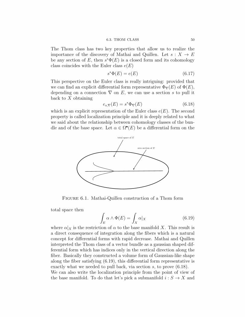
6.3. THOM CLASS 50
The Thom class has two key properties that allow us to realize theimportance of the discovery of Mathai and Quillen. Let s : X → Ebe any section of E, then s∗Φ(E) is a closed form and its cohomologyclass coincides with the Euler class e(E)
s∗Φ(E) = e(E) (6.17)
This perspective on the Euler class is really intriguing: provided thatwe can find an explicit differential form representative Φ∇(E) of Φ(E),depending on a connection ∇ on E, we can use a section s to pull itback to X obtaining
es,∇(E) = s∗Φ∇(E) (6.18)
which is an explicit representation of the Euler class e(E). The secondproperty is called localization principle and it is deeply related to whatwe said about the relationship between cohomology classes of the bun-dle and of the base space. Let α ∈ Ω•(E) be a differential form on the
Figure 6.1. Mathai-Quillen construction of a Thom form
total space then
E
α ∧ Φ(E) =
X
α|X (6.19)
where α|X is the restriction of α to the base manifold X. This result isa direct consequence of integration along the fibers which is a naturalconcept for differential forms with rapid decrease. Mathai and Quilleninterpreted the Thom class of a vector bundle as a gaussian shaped dif-ferential form which has indices only in the vertical direction along thefiber. Basically they constructed a volume form of Gaussian-like shapealong the fiber satisfying (6.19), this differential form representative isexactly what we needed to pull back, via section s, to prove (6.18).We can also write the localization principle from the point of view ofthe base manifold. To do that let’s pick a submanifold i : S → X and
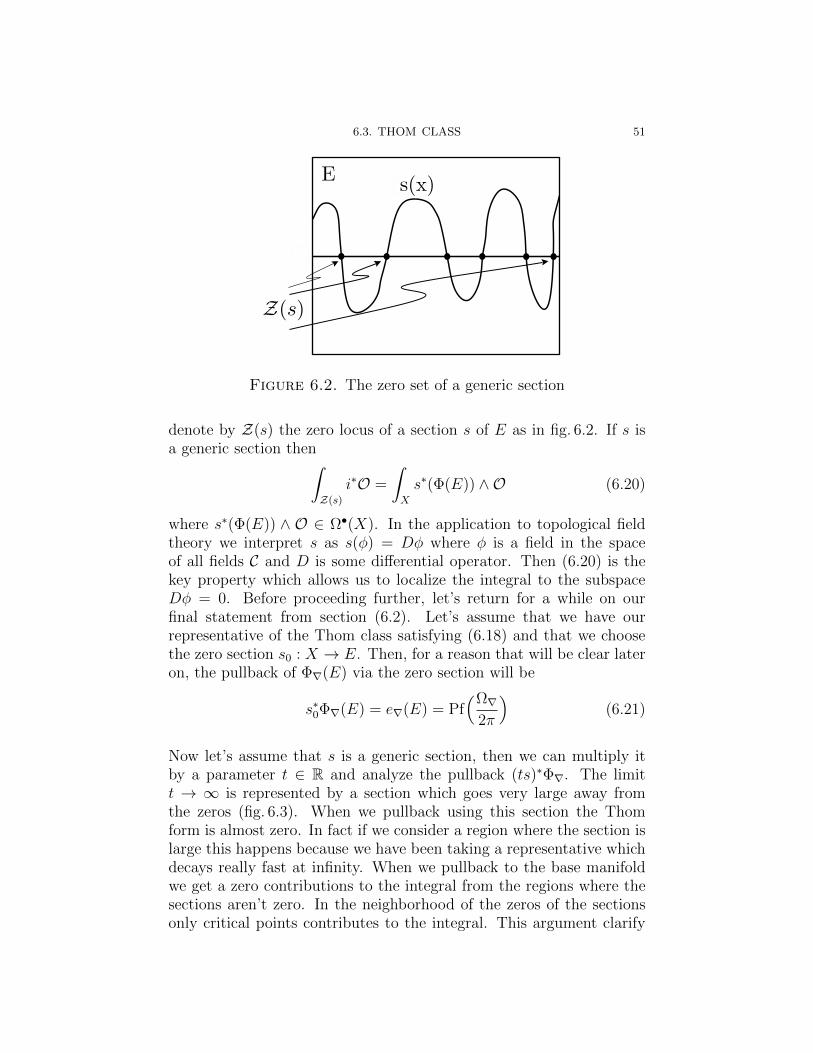
6.3. THOM CLASS 51
Figure 6.2. The zero set of a generic section
denote by Z(s) the zero locus of a section s of E as in fig. 6.2. If s isa generic section then
Z(s)
i∗O =
X
s∗(Φ(E)) ∧O (6.20)
where s∗(Φ(E)) ∧ O ∈ Ω•(X). In the application to topological fieldtheory we interpret s as s(φ) = Dφ where φ is a field in the spaceof all fields C and D is some differential operator. Then (6.20) is thekey property which allows us to localize the integral to the subspaceDφ = 0. Before proceeding further, let’s return for a while on ourfinal statement from section (6.2). Let’s assume that we have ourrepresentative of the Thom class satisfying (6.18) and that we choosethe zero section s0 : X → E. Then, for a reason that will be clear lateron, the pullback of Φ∇(E) via the zero section will be
s∗0Φ∇(E) = e∇(E) = PfΩ∇
2π
(6.21)
Now let’s assume that s is a generic section, then we can multiply itby a parameter t ∈ R and analyze the pullback (ts)∗Φ∇. The limitt → ∞ is represented by a section which goes very large away fromthe zeros (fig. 6.3). When we pullback using this section the Thomform is almost zero. In fact if we consider a region where the section islarge this happens because we have been taking a representative whichdecays really fast at infinity. When we pullback to the base manifoldwe get a zero contributions to the integral from the regions where thesections aren’t zero. In the neighborhood of the zeros of the sectionsonly critical points contributes to the integral. This argument clarify
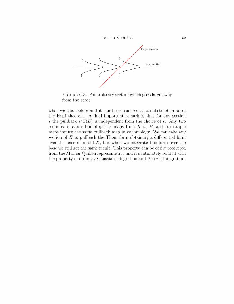
6.3. THOM CLASS 52
Figure 6.3. An arbitrary section which goes large awayfrom the zeros
what we said before and it can be considered as an abstract proof ofthe Hopf theorem. A final important remark is that for any sections the pullback s∗Φ(E) is independent from the choice of s. Any twosections of E are homotopic as maps from X to E, and homotopicmaps induce the same pullback map in cohomology. We can take anysection of E to pullback the Thom form obtaining a differential formover the base manifold X, but when we integrate this form over thebase we still get the same result. This property can be easily recoveredfrom the Mathai-Quillen representative and it’s intimately related withthe property of ordinary Gaussian integration and Berezin integration.
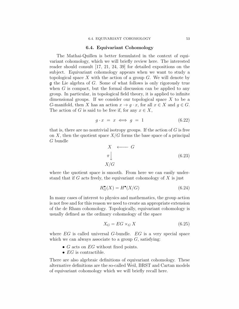
6.4. EQUIVARIANT COHOMOLOGY 53
6.4. Equivariant Cohomology
The Mathai-Quillen is better formulated in the context of equi-variant cohomology, which we will briefly review here. The interestedreader should consult [17, 21, 24, 39] for detailed expositions on thesubject. Equivariant cohomology appears when we want to study atopological space X with the action of a group G. We will denote byg the Lie algebra of G. Some of what follows is only rigorously truewhen G is compact, but the formal discussion can be applied to anygroup. In particular, in topological field theory, it is applied to infinitedimensional groups. If we consider our topological space X to be aG-manifold, then X has an action x → g · x, for all x ∈ X and g ∈ G.The action of G is said to be free if, for any x ∈ X,
g · x = x ⇐⇒ g = 1 (6.22)
that is, there are no nontrivial isotropy groups. If the action of G is freeon X, then the quotient space X/G forms the base space of a principalG bundle
X ←−−− G
π
X/G
(6.23)
where the quotient space is smooth. From here we can easily under-stand that if G acts freely, the equivariant cohomology of X is just
H•G(X) = H•(X/G) (6.24)
In many cases of interest to physics and mathematics, the group actionis not free and for this reason we need to create an appropriate extensionof the de Rham cohomology. Topologically, equivariant cohomology isusually defined as the ordinary cohomology of the space
XG = EG×G X (6.25)
where EG is called universal G-bundle. EG is a very special spacewhich we can always associate to a group G, satisfying:
• G acts on EG without fixed points.• EG is contractible.
There are also algebraic definitions of equivariant cohomology. Thesealternative definitions are the so-called Weil, BRST and Cartan modelsof equivariant cohomology which we will briefly recall here.
6.4. EQUIVARIANT COHOMOLOGY 54
6.4.1. Weil Model. In the study of the differential geometry ofa principal bundle P with Lie algebra g we encounter the so-calledWeil algebra W(g). Let us recall its definition; for more details see,for example, [21]. The Weil algebra is a dg-algebra, see (4.2), withg-valued generators ω,φ of degrees 1 and 2 respectively. We define adifferential operator dW which acts on the generators as
dWω = φ−1
2[ω,ω] dWφ = −[ω,φ] (6.26)
It may be seen that dW is nilpotent, d2W = 0. These are the relationsthat are valid for a connection ω and curvature φ on a principal bundleP . Basically we can interpret φ and ω as algebraic counterparts of thecurvature and the connection. Moreover, we can define a connectionsimply as a homomorphism W(g) → Ω•(P ). We can also introduce twoderivations of the Weil algebra: the interior derivative or contraction
ιaωb = δba ιaφ
b = 0 (6.27)
(where ω = ωaea,φ = φaea, with ea a basis for g) and the Lie derivative
La = ιadW + dWιa (6.28)
For the Weil model of equivariant cohomology we consider the algebraW(g)⊗Ω•(X). Algebraically, the replacement X → EG×X is analo-gous to Ω(X) → W(g)⊗ Ω(X). On this algebra we have the action ofthe operators ιa and La, now defined as ιa = ιa ⊗ 1 + 1⊗ ιa etc. Herewe write ιa = ι(Va), with Va the vector field on X corresponding to theLie algebra element ea. One then restricts to the so-called basic formsη ∈ W(g)⊗ Ω∗(X) which satisfy ιaη = Laη = 0. Basic forms are hori-zontal and G-invariant differential forms. The equivariant cohomologygroups are then defined as
H•G(X) = H•((W(g)⊗ Ω•(X))basic, dT ) (6.29)
wheredT = dW ⊗ 1 + 1⊗ d (6.30)
is the differential.
6.4.2. Cartan Model. Following what we did previously, we startby defining the Cartan algebra C(g) which is obtained by simply puttingω = 0 in the Weil algebra and is generated by the single variable φof degree two. The Cartan model is a simpler model of equivariantcohomology based on the Cartan algebra C(g) = S(g∗). The startingpoint is now the algebra S(g∗)⊗ Ω•(X), but as differential we choose
dC = 1⊗ d− φa⊗ ιa. (6.31)
6.5. UNIVERSAL THOM CLASS 55
This operator satisfies (dC)2 = −φa⊗La and thus only defines a complexon theG-invariant forms. The Cartan model of equivariant cohomologyis now defined as
H•G(X) = H•((S(g∗)⊗ Ω•(X))G, dC). (6.32)
It is possible to show that the definitions (6.29) and (6.32) are equiv-alent and agree with the topological definition. This last statement isbest understood in the context of the so-called BRST model of equi-variant cohomology and it was originally shown by Kalkman in [23, 24].
6.5. Universal Thom Class
We will now show how to construct a nice explicit representativefor Φ(E) by first constructing a “universal” representative [17]. WhileE might be twisted and difficult to work with, we can replace construc-tions on E by equivariant constructions on a trivial bundle. Let E bean orientable real vector bundle such that rk(E) = 2m, with standardfiber V . Since E is orientable the structure group G of the bundle canbe reduced to SO(V ) and we will denote its Lie algebra by gs. We canidentify E as a bundle associated to a principal SO(V ) bundle P → X,where P is the SO(V ) bundle of all orthonormal oriented frames on E
π : P × V → E =P × V
G(6.33)
Recall that when given a principal G-bundle π : P → X, a differentialform α on P descends to a form on X if the following two conditions aresatisfied: first, given vector fields Vi , α(V1, . . . , Vq) = 0 whenever oneof the Vi is vertical. In this case α is said to be horizontal. Second, α isinvariant under the G action. The forms that satisfy both conditionsare called basic. We already encountered basic differential forms in(6.4.1). In particular, if we consider the principal bundle (6.33) wehave an isomorphism
Ω•(P ×G V ) Ω•(P × V )basic (6.34)
Suppose now that P is endowed with a connection A ∈ Ω1(P, gs) andassociated curvature Ω ∈ Ω2(P, gs), and consider the Weil algebra,W(gs). As gs = so(2m) the generators are antisymmetric matricesAab (of degree 1) and Ωab (of degree 2). The property that W(g)provides a universal realization of the relations defining the curvatureand connection on P gives the Chern-Weil homomorphism
w : W(g) → Ω•(P ) (6.35)

6.5. UNIVERSAL THOM CLASS 56
defined in a natural way through the expansions
A = AαTα Ω = ΩαTα (6.36)
where Tαα=1,...,dim(G) is a basis of g, and Aα ∈ Ω1(P ), Ωα ∈ Ω2(P ).For G = SO(2m), the map w is just the correspondence between thegenerators of W(gs) and the entries of the antisymmetric matrices forthe curvature and connection in P . The Chern-Weil homomorphismmaps the universal connection and curvature in the Weil algebra tothe actual connection and curvature in P . Combined with the liftingof forms from V to P × V , we obtain another homomorphism
w ⊗ π∗2 : W(g)⊗ Ω•(V ) → Ω•(P × V ) (6.37)
where π2 : P × V → V is the projection on the second factor. This isthe geometric context of the Mathai-Quillen construction and the cor-respondence between the de Rham theory on P and the Weil algebra,W(gs), suggests the following definition.
Definition 6.5.1. A form U ∈ W(gs) ⊗ Ωrd(V ) will be called a uni-versal Thom form (in the Weil model) if it satisfies:
(i) U is basic(ii) QU = 0, where Q = dW + d(iii)
V U = 1
The reason U is useful is that if we choose a connection ∇ on Ecompatible with the fiber metric, then we can obtain a representativeΦ∇(E) of the Thom class as follows. As we have noted, a connectionon E, (equivalently, a connection on P ) is the same thing as a choiceof Weil homomorphism w : W(gs) → Ω•(P ). We then have a diagram:
W(gs)⊗ Ω•(V )w⊗π∗
2 > Ω•(P × V )
(W(gs)⊗ Ω•(V ))basic
∧
w⊗π∗2
> Ω•(P × V )basic
∧
Ω•(E)
π∗∧
w>
(6.38)
Applying the Weil homomorphism combined with the lifting of forms,w ⊗ π∗
2, to U ∈ W(gs)⊗ Ω•(V ) gives (w ⊗ π∗2)(U) ∈ Ω•(P × V ). This
form is then a basic closed differential form which descends to a formin Ω•(E) , that is,
Φ∇(E) = w(U) (6.39)
6.6. MATHAI-QUILLEN REPRESENTATIVE OF THE THOM CLASS 57
for some form Φ∇(E) ∈ H2mrd (E). Using the defining properties of the
Thom class of E described in (6.3), we see that properties (i), (ii) and(iii) suffice to prove that w(U) represents the Thom class of E. Finally,we have used here the Weil model of equivariant cohomology but it isalso possible to construct a universal class in the Cartan or BRSTmodel. For more details, see [21].
6.6. Mathai-Quillen Representative of the Thom Class
The universal Thom form U of Mathai and Quillen is an elementin W(gs)⊗ Ω•(V ) given by
U = (2π)−mPf(Ω) exp
−
1
2ξ2 −
1
2∇ξa(Ω−1)ab∇ξb
(6.40)
In this expression the ξa are fiber coordinates on V , ∇ξa is the exteriorcovariant derivative of ξa such that ∇ξa = dξa + Aa
bξb and Ωab, Aab
are the antisymmetric matrices of generators in W(gs). As we can see,U is SO(V ) invariant, then a necessary condition for (i) is that U behorizontal. This is achieved by inserting the covariant derivative, infact ∇ξ is horizontal
ι(Va)∇ξa = 0 (6.41)
so U is horizontal. Thus, U is basic, checking property (i). In theuniversal Thom form the Ω−1 is slightly formal, but makes perfectlysense if we expand the exponential and we combine with the Pfaffian.In this way we get a volume form on the fiber which is what we need tointegrate. As stated in [17] the curvature matrix is never invertible in ageometric situation. Nevertheless, by introducing the Weil algebra andequivariant forms, we can obtain a universal algebraic situation wherethe curvature matrix can be assumed invertible. To prove the remaingproperties it’s convenient to take into account another representationof the universal Thom form based on Berezin integration. The Pfaffianof a real antisymmetric matrix Kab can be written as
Pf(K) =
dχ expχaK
abχb/2 (6.42)
where χa is a real odd variable. See section (2.5). It is easy to writethe universal Thom form as
U = (2π)−m
dχ exp−ξ2/2 + χaΩ
abχb/2 + i∇ξaχa (6.43)
and the expansion of this expression leads precisely to (6.40). Fromthis representation it is obvious that
V U = 1. The reason is that to
get a top form on V we have to take the term in the exponential with
6.6. MATHAI-QUILLEN REPRESENTATIVE OF THE THOM CLASS 58
the top degree of dξ. This also pulls off the top form in χ. Then, sincethe χ and dξa anticommute
V
U =1
(2π)m
V
dχ e−ξ2/2 i2m
(2m)!
dξaχa
2m
=1
(2π)m
V
dξ1 ∧ · · · ∧ dξ2m e−ξ2/2 = 1
(6.44)
It remains to show that U is closed. In order to write a manifestly closedexpression for U we enlarge the equivariant cohomology complex to
W(gs)⊗ Ω•(V )⊗ Ω•(ΠV ∗) (6.45)
and consider the following differential
QW = dW ⊗ 1⊗ 1 + 1⊗ d⊗ 1 + 1⊗ 1⊗ δ (6.46)
dW is the Weil differential defined in (6.4.1), while δ is the de Rhamdifferential in ΠV ∗. To do that we first introduce an auxiliary bosonicfield Ba, which has the meaning of a basis of differential forms for thefiber. In this way we have a pair of fields (χa, Ba) associated to thefiber V . The action of δ on this fields is explicitly
δ
χa
Ba
=
0 10 0
χa
Ba
(6.47)
Notice that Q2W = 0. Expanding the action and doing the Gaussian
integral on B leads to the representation
U =1
(2π)2m
dχdBe−QW (Ψ) (6.48)
where the so called “gauge fermion” is given by
Ψ = χa(iξa +
1
4Aabχb +
1
2Ba) (6.49)
Acting with δ on Ψ we get
δΨ = Ba∂Ψ
∂χa(6.50)
then
QWΨ = (dW + d)Ψ+Ba∂Ψ
∂χa(6.51)
We can get rid of the δ-action on Ψ because it produces a term whichis a total derivative with respect to χ and this term integrates to zero
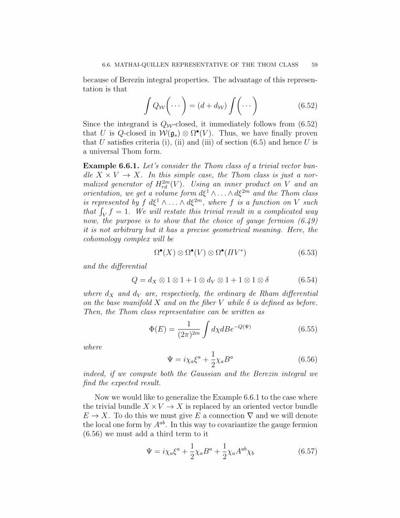
6.6. MATHAI-QUILLEN REPRESENTATIVE OF THE THOM CLASS 59
because of Berezin integral properties. The advantage of this represen-tation is that
QW
· · ·
= (d+ dW)
· · ·
(6.52)
Since the integrand is QW-closed, it immediately follows from (6.52)that U is Q-closed in W(gs) ⊗ Ω•(V ). Thus, we have finally proventhat U satisfies criteria (i), (ii) and (iii) of section (6.5) and hence U isa universal Thom form.
Example 6.6.1. Let’s consider the Thom class of a trivial vector bun-dle X × V → X. In this simple case, the Thom class is just a nor-malized generator of H2m
rd (V ). Using an inner product on V and anorientation, we get a volume form dξ1 ∧ . . .∧ dξ2m and the Thom classis represented by f dξ1 ∧ . . . ∧ dξ2m, where f is a function on V suchthat
V f = 1. We will restate this trivial result in a complicated way
now, the purpose is to show that the choice of gauge fermion (6.49)it is not arbitrary but it has a precise geometrical meaning. Here, thecohomology complex will be
Ω•(X)⊗ Ω•(V )⊗ Ω•(ΠV ∗) (6.53)
and the differential
Q = dX ⊗ 1⊗ 1 + 1⊗ dV ⊗ 1 + 1⊗ 1⊗ δ (6.54)
where dX and dV are, respectively, the ordinary de Rham differentialon the base manifold X and on the fiber V while δ is defined as before.Then, the Thom class representative can be written as
Φ(E) =1
(2π)2m
dχdBe−Q(Ψ) (6.55)
where
Ψ = iχaξa +
1
2χaB
a (6.56)
indeed, if we compute both the Gaussian and the Berezin integral wefind the expected result.
Now we would like to generalize the Example 6.6.1 to the case wherethe trivial bundle X×V → X is replaced by an oriented vector bundleE → X. To do this we must give E a connection ∇ and we will denotethe local one form by Aab. In this way to covariantize the gauge fermion(6.56) we must add a third term to it
Ψ = iχaξa +
1
2χaB
a +1
2χaA
abχb (6.57)
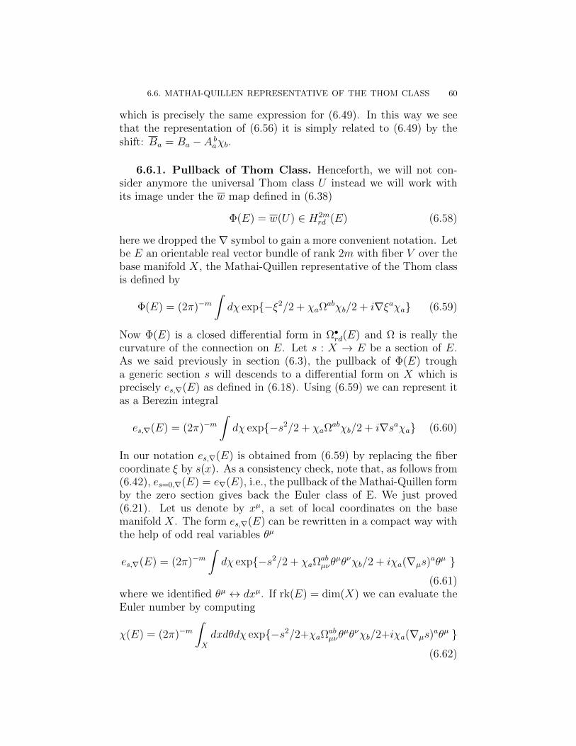
6.6. MATHAI-QUILLEN REPRESENTATIVE OF THE THOM CLASS 60
which is precisely the same expression for (6.49). In this way we seethat the representation of (6.56) it is simply related to (6.49) by theshift: Ba = Ba − A b
aχb.
6.6.1. Pullback of Thom Class. Henceforth, we will not con-sider anymore the universal Thom class U instead we will work withits image under the w map defined in (6.38)
Φ(E) = w(U) ∈ H2mrd (E) (6.58)
here we dropped the ∇ symbol to gain a more convenient notation. Letbe E an orientable real vector bundle of rank 2m with fiber V over thebase manifold X, the Mathai-Quillen representative of the Thom classis defined by
Φ(E) = (2π)−m
dχ exp−ξ2/2 + χaΩ
abχb/2 + i∇ξaχa (6.59)
Now Φ(E) is a closed differential form in Ω•rd(E) and Ω is really the
curvature of the connection on E. Let s : X → E be a section of E.As we said previously in section (6.3), the pullback of Φ(E) trougha generic section s will descends to a differential form on X which isprecisely es,∇(E) as defined in (6.18). Using (6.59) we can represent itas a Berezin integral
es,∇(E) = (2π)−m
dχ exp−s2/2 + χaΩ
abχb/2 + i∇saχa (6.60)
In our notation es,∇(E) is obtained from (6.59) by replacing the fibercoordinate ξ by s(x). As a consistency check, note that, as follows from(6.42), es=0,∇(E) = e∇(E), i.e., the pullback of the Mathai-Quillen formby the zero section gives back the Euler class of E. We just proved(6.21). Let us denote by xµ, a set of local coordinates on the basemanifold X. The form es,∇(E) can be rewritten in a compact way withthe help of odd real variables θµ
es,∇(E) = (2π)−m
dχ exp−s2/2 + χaΩ
abµνθ
µθνχb/2 + iχa(∇µs)aθµ
(6.61)where we identified θµ ↔ dxµ. If rk(E) = dim(X) we can evaluate theEuler number by computing
χ(E) = (2π)−m
X
dxdθdχ exp−s2/2+χaΩabµνθ
µθνχb/2+iχa(∇µs)aθµ
(6.62)
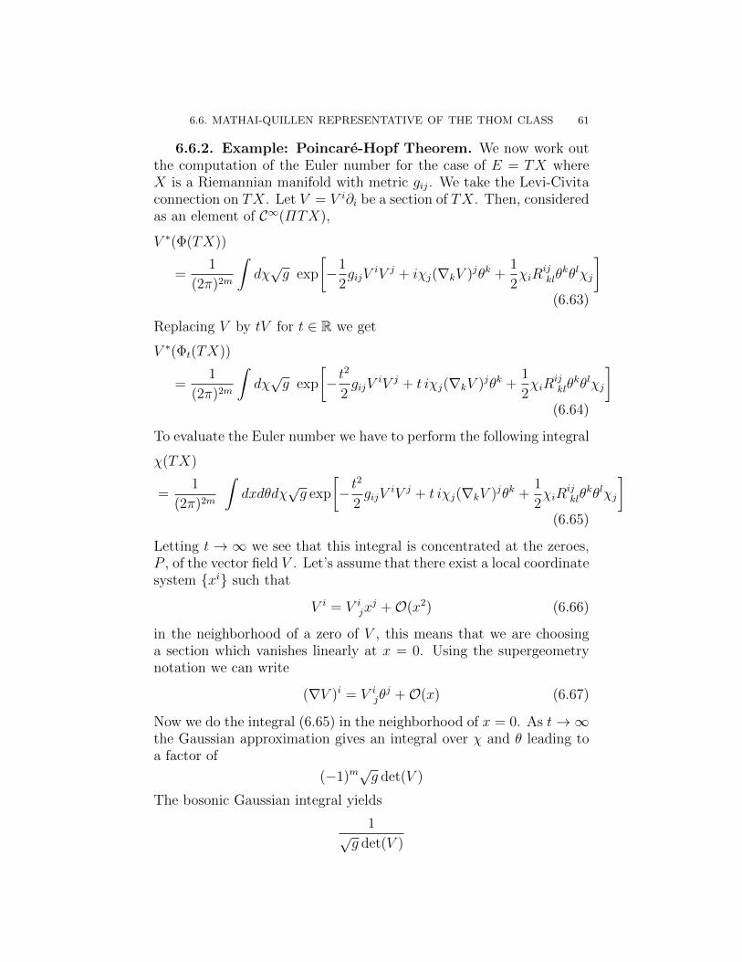
6.6. MATHAI-QUILLEN REPRESENTATIVE OF THE THOM CLASS 61
6.6.2. Example: Poincare-Hopf Theorem. We now work outthe computation of the Euler number for the case of E = TX whereX is a Riemannian manifold with metric gij. We take the Levi-Civitaconnection on TX. Let V = V i∂i be a section of TX. Then, consideredas an element of C∞(ΠTX),
V ∗(Φ(TX))
=1
(2π)2m
dχ
√g exp
−1
2gijV
iV j + iχj(∇kV )jθk +1
2χiR
ijklθ
kθlχj
(6.63)
Replacing V by tV for t ∈ R we get
V ∗(Φt(TX))
=1
(2π)2m
dχ
√g exp
−t2
2gijV
iV j + t iχj(∇kV )jθk +1
2χiR
ijklθ
kθlχj
(6.64)
To evaluate the Euler number we have to perform the following integral
χ(TX)
=1
(2π)2m
dxdθdχ
√g exp
−t2
2gijV
iV j + t iχj(∇kV )jθk +1
2χiR
ijklθ
kθlχj
(6.65)
Letting t → ∞ we see that this integral is concentrated at the zeroes,P , of the vector field V . Let’s assume that there exist a local coordinatesystem xi such that
V i = V ijx
j +O(x2) (6.66)
in the neighborhood of a zero of V , this means that we are choosinga section which vanishes linearly at x = 0. Using the supergeometrynotation we can write
(∇V )i = V ijθ
j +O(x) (6.67)
Now we do the integral (6.65) in the neighborhood of x = 0. As t → ∞
the Gaussian approximation gives an integral over χ and θ leading toa factor of
(−1)m√g det(V )
The bosonic Gaussian integral yields
1√g det(V )
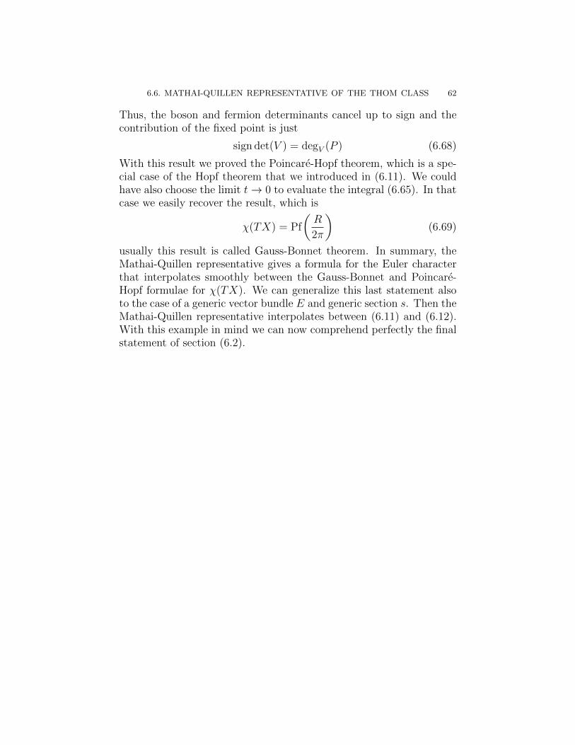
6.6. MATHAI-QUILLEN REPRESENTATIVE OF THE THOM CLASS 62
Thus, the boson and fermion determinants cancel up to sign and thecontribution of the fixed point is just
sign det(V ) = degV (P ) (6.68)
With this result we proved the Poincare-Hopf theorem, which is a spe-cial case of the Hopf theorem that we introduced in (6.11). We couldhave also choose the limit t → 0 to evaluate the integral (6.65). In thatcase we easily recover the result, which is
χ(TX) = Pf
R
2π
(6.69)
usually this result is called Gauss-Bonnet theorem. In summary, theMathai-Quillen representative gives a formula for the Euler characterthat interpolates smoothly between the Gauss-Bonnet and Poincare-Hopf formulae for χ(TX). We can generalize this last statement alsoto the case of a generic vector bundle E and generic section s. Then theMathai-Quillen representative interpolates between (6.11) and (6.12).With this example in mind we can now comprehend perfectly the finalstatement of section (6.2).
CHAPTER 7
BV representative of the Thom Class
The goal of this section is to formulate a new representative ofthe Thom class using the ideas of BV formalism. In particular, toachieve this result, we will apply the odd Fourier transform definedin (5.1). From a mathematical point of view, we are defining the oddFourier transform for differential forms on vector bundles and obtainingconsequently representatives for the Thom class of arbitrary vectorbundles. This problem was raised in a paper by Kalkman [23] and thissection can be seen as a solution to that.
7.1. Geometry of T [1]E
Let be E an orientable real vector bundle of rank 2m with fiber Vover the base manifold X, as we already seen in (6.6.1) the Mathai-Quillen representative of the Thom class is defined by
Φ(E) = (2π)−m
dχ exp−ξ2/2 + χaΩ
abχb/2 + i∇ξaχa (7.1)
where ξ’s are fiber coordinates, χ’s are fermionic variables and ∇ξa
is the exterior covariant derivative of ξa. The presence of covariantderivative may sound strange since to integrate Φ(E) along the fiberswe just need to put a term of the form dξaχa in the exponential inorder to get a top form on Ω•(V ). The problem of a term like this, inthe formula above, is that it will affect the covariance. Both ξ and χtransforms as a section but dξ not, in fact
ξa = tab (x)ξb⇒ dξa = ∂µt
ab (x)dx
µξb + tab (x)dξb (7.2)
Before proceeding further, we have to clarify one point. In the studyof differential geometry on total space of a vector bundle E → X wewould like to divide up the coordinates into two sets: basic coordinatesxµ and fiber coordinates ξa. Similarly, the anticommuting variablesseparate into θµ = dxµ and λa = dξa. At this point it is very con-venient to employ the extra data of a connection ∇ on E to restorethe covariance for the action of the differential d on T [1]E. In thiscontext T [1]E is the graded manifold that we can naturally associateto E and following Example 4.2.2 we will identify smooth functions on
63
7.2. ODD FOURIER TRANSFORM REVISITED 64
T [1]E with differential forms on E, C∞(T [1]E) = Ω•(E). Using theconnection ∇ we can establish the following isomorphism
T [1]E E ⊕ E[1] ⊕ T [1]M
(xµ, ξa)∨
λa∨
θµ∨
(7.3)
where λa is the new anticommuting fiber coordinates that transformsas a section of E. Following [27], what we just did is a reduction ofthe structure group of the sheaf of functions on T [1]E by means of aconnection. In this way, our sheaf of functions will be generated by vari-ables (xµ, θµ; ξa,λa) with (θµ; ξa,λa) transforming linearly across patchboundaries on the base manifold X. So, we can write out explicitly theaction of the differential on the variables as
dxµ = θµ
dθµ = 0
∇ξa ≡ λa = dξa + Aaµ bθ
µξb
∇λa = dλa + Aaµ bθ
µλb = 12Ω
abµνθ
µθνξb
(7.4)
where Aaµ b is the local expression for the connection 1-form and Ωa
bµν
is the local expression for the curvature 2-form. Summarizing, we dis-covered that in the case of the total space of a vector bundle, the fibervariable λa should be considered as the covariant differential ∇ξa.
7.2. Odd Fourier Transform Revisited
Let’s consider all the notations introduced in (7.1), the form Φ(E)can be rewritten as
Φ(E) = (2π)−m
dχ exp−ξ2/2 + χaΩ
abµνθ
µθνχb/2 + iλaχa (7.5)
It is helpful to consider also the following notation
Φ(E) = (2π)−m
dχ exp(Ψ) (7.6)
whereΨ = −ξ2/2 + χaΩ
abµνθ
µθνχb/2 + iλaχa (7.7)
From the point of view of the base manifold X, the odd Fourier trans-form is a way to relate T [1]X and T ∗[−1]X, see (5.1). In this sub-section, we would like to look at the odd Fourier transform from thepoint of view of total space E and think of it as a tool to relate T [1]Eand T ∗[−1]E. Again, in the study of T ∗[−1]E it is useful to reducethe structure group of the the sheaf of functions using the extra data
7.2. ODD FOURIER TRANSFORM REVISITED 65
of the connection previously introduced. We create the following iso-morphism
T ∗[−1]E E ⊕ E∗[−1] ⊕ T ∗[−1]M
(xµ, ξa)∨
σa
∨ψµ
∨(7.8)
where σa is the dual variable with respect to λa introduced in (7.1). Itis important to stress that (7.3) and (7.8) are examples of non canon-ical splitting, these splittings are possible only upon the choice of aconnection ∇. Thus, the generalization of odd Fourier transform fordifferential forms on a vector bundle will maps functions on T [1]E tofunctions on T ∗[−1]E
F : C∞(T [1]E) → C∞(T ∗[−1]E) (7.9)
and the corresponding action on the coordinates will be
(xµ, θµ; ξa,λa)F−→ (xµ,ψµ; ξ
a, σa) (7.10)
Being a differential forms on E, the Mathai-Quillen representative (7.5)can be identified with a smooth functions on T [1]E
Φ(E) ∈ C∞(T [1]E) (7.11)
then it is natural to ask how it would look the odd Fourier transformof Φ(E). Precisely, we have
F [Φ(E)] = ΦBV (E) = (2π)−m
dθρ(x)−1
dλρ(ξ)−1
dχ expΨ
(7.12)where Ψ is expressed as
Ψ = −ξ2/2 + 12χaΩab
µνθµθνχb − iχaλa + ψµθµ + σaλa (7.13)
After some manipulation, it is possible to show that
ΦBV (E) = (2π)−m
dθρ−1
x ρ−1ξ exp−ξ2/2 + σaΩ
abµνθ
µθνσb/2 + ψµθµ
(7.14)From now on, we will refer to ΦBV (E) as the BV representative for theThom class of the vector bundle E which should be considered as asmooth functions on T ∗[−1]E. The expression (7.13) transforms nicelybecause of the covariantization procedure that we adopted. In conclu-sion, we have seen that providing a generalization of the odd Fouriertransform to the case of a vector bundle we can define a new Thomclass representative which is the BV representative ΦBV (E) defined in(7.12).
7.3. ANALYSIS OF THE BV REPRESENTATIVE 66
7.3. Analysis of the BV Representative
Looking at the explicit expression for ΦBV (E) it appears clearlythat we have a rapid decay object, which integrates to 1 upon properBerezin integrations. However, to be sure that the procedure that wefollowed to contruct this new representative is correct we have to checkall the properties in the definition of the Thom class i.e. we have tocheck that ΦBV (E) is closed which is less evident. At this stage it isworth to spend some words to prove that also the MQ representativeΦ(E) is closed.
Proof. The standard exterior derivative, acting on Ω(E), will looklike
D = dxµ ∂
∂xµ+ dξa
∂
∂ξa(7.15)
Observing what we described in (7.1), the convenient way to expressD is really
D = θµ∂
∂xµ− Aa
µ bθµξb
∂
∂ξa+ λa ∂
∂ξa= ∇+ λa ∂
∂ξa(7.16)
where ∇ is the usual covariant derivative. In this way we get
DΦ(E) = (2π)−m
dχ exp(Ψ)
∇Ψ+ λa ∂Ψ
∂ξa
(7.17)
then
λa ∂Ψ
∂ξa= −ξaλ
a
∇Ψ = +i∇νAaµ bθ
µθνξbχa = −iξaΩabµνθ
µθνχb
(7.18)
and
∇Ψ+ λa ∂Ψ
∂ξa= −ξaλ
a− iξaΩ
abµνθ
µθνχb (7.19)
where we used the Bianchi identities ∇Ω = 0,∇A = Ω and the anti-symmetry of Ωab. Using the properties of Berezin integration we canalways write
Φ(E) = (2π)−m
dχ exp(Ψ) + (2π)−m
dχ
∂
∂χexp(Ψ) (7.20)
since the last term integrates to zero. At this point we can express(7.17) as
DΦ(E) = (2π)−m
dχ exp(Ψ)
− ξaλ
a− iξaΩ
abµνθ
µθνχb + iξa∂Ψ
∂χa
= 0(7.21)
7.3. ANALYSIS OF THE BV REPRESENTATIVE 67
indeed
iξa∂Ψ
∂χa= ξaλ
a + iξaΩabµνθ
µθνχb (7.22)
In this way we proved that Φ(E) is a closed differential form, as itshould be, since this is a defining property for the Thom class.
To show that ΦBV (E) is closed we cannot simply apply the operatorD but we have to transform it to get the proper differential operator onT ∗[−1]E. Doing that, we will obtain an odd Laplacian operator thatwe will denote ∆BV . The Fourier transformation for (7.16) will be
∆BV =∂2
∂xµ∂ψµ− Aa
µ bξb ∂2
∂ψµ∂ξa+
∂2
∂ξa∂σa(7.23)
It is not difficult to understand how we got this formula indeed wefollowed the same considerations of (5.1). However, for the sake ofsimplicity, here we assumed that all the ρ’s are constant. Thus, alsoΦBV (E) is closed in fact
Proof. By (5.8) we know that
∆BV F [Φ(E)] = F [DΦ(E)] (7.24)
To verify this statement we firstly calculate the following expression
∆BV exp(Ψ) = exp(Ψ)
∂Ψ∂xµ
∂Ψ∂ψµ
− Aaµ bξ
b ∂Ψ∂ξa
∂Ψ∂ψµ
+∂Ψ∂ξa
∂Ψ∂σa
= exp(Ψ)
θµ
∂Ψ∂xµ
− Aaµ bθ
µξb∂Ψ∂ξa
+ λa ∂Ψ∂ξa
= exp(Ψ)(DΨ)
(7.25)
then we have
∆BV F [Φ(E)] = (2π)−m
dθρ(x)−1
dλρ(ξ)−1
dχ∆BV exp(Ψ)
= (2π)−m
dθρ(x)−1
dλρ(ξ)−1
dχ exp(Ψ)(DΨ)
= F [DΦ(E)] = 0(7.26)
where the last equality follows from (7.21). Finally, the BV representative ΦBV (E) is effectively a representa-
tive for the Thom class of E. In the language of BV quantization,introduced in (5.4.1), the fact that ΦBV (E) is closed mean that wehave found a solution to the master equation. The outcome of this sec-tion is that we have found a nice relationship between two seemingly

7.3. ANALYSIS OF THE BV REPRESENTATIVE 68
unrelated subjects such as the BV formalism and the Mathai-Quillenformalism.
CHAPTER 8
Conclusions
The focus of this thesis was the construction of a new representative,for the Thom class of a vector bundle, called BV representative. Thisrepresentative has been constructed using the odd Fourier transformdeveloped in [15, 23]. In (7.1) and (7.2) we shown how it is possibleto generalize the odd Fourier transform to the case of a vector bundle.Considering the MQ Thom form as a smooth function over T [1]E, weobtained the corresponding BV representative defined over T ∗[−1]E.In (7.3) we also shown that our BV representative is closed under theaction of a suitable differential operator, this means that the BV rep-resentative is a solution to the BV master equation. In view of theseresults, chapter 7 is a proof for the following theorem
Theorem 8.0.1. The BV representative ΦBV (E) is a multivectorfield representative for the Thom class of a vector bundle and it is asolution to the BV master equation.
The present work can be seen as a first step in the process of un-derstanding BV quantization from the point of view of Mathai-Quillenformalism. Indeed, on one hand we have the MQ construction whichis a concrete prescription that can be used to calculate Euler class andits infinite dimensional generalization is very well understood, beingthe basis of all cohomological topological field theories. On the otherhand we have the BV quantization which is, algebraically, a very pow-erful technique but we still have a lack of knowledge on what we areeffectively computing in this formalism. Moreover, the path integralmanipulations in BV formalism are understood only formally and thefinite dimensional setting provides only a good heuristically compre-hension of the problem. Understanding completely BV quantization isa very deep problem, far beyond the aim of this thesis, but it is also afertile ground for future investigations and interesting discoveries.
69
8. CONCLUSIONS 70
Acknowledgments There are a lot of people to thank. First of all, Iwant to express my gratitude to my supervisor Maxim Zabzine. It wasa great pleasure to learn from him. Not only because of his ability toexplain difficult things in an easy way, but also experiencing his wayof thinking, has been very stimulating. Likewise, it is a pleasure tothank my official supervisor Roberto Zucchini. Thanks for always be-ing interested in my progress, for helpful discussions and for the recom-mendation letters. Moreover, thanks to Francesco Bonechi for takingthe time to read my thesis and to answer my questions. More gener-ally, thanks to all the people who contributed to my understanding ofmathematics and physics. Of course, I would also like to thank Da-vide Bianchini, Luca Zambelli, Luca Boccioletti, Stefano Evangelisti,Luca Taddia, Lorenzo Cevolani, Paolo Mattioli, Riccardo Colabraro,Jacob Winding, Anton Nedelin, Giuseppe Dibitetto and Raul Pereira.I greatly benefited from all our discussions. Finally, my gratitude goesout to my family, who always have encouraged and supported me inmy education, and my friends. Thank you all!
Bibliography
[1] E. Witten, “Notes On Supermanifolds and Integration,”arXiv:1209.2199 [hep-th].
[2] F. A. Berezin, Introduction To Superanalysis, A. A. Kirillov, ed.(D. Reidel, 1987).
[3] Yu. I. Manin, Gauge Field Theory And Complex Geometry(Springer-Verlag, 1988).
[4] B. DeWitt, Supermanifolds, second edition (Cambridge UniversityPress, 1992).
[5] P. Deligne and J. W. Morgan, “Notes On Supersymmetry (follow-ing Joseph Bernstein),” in P. Deligne et. al., eds., Quantum FieldsAnd Strings: A Course For Mathematicians, Vol. 1 (AmericanMathematical Society, 1999).
[6] I. A. Batalin and G. A. Vilkovisky, “Gauge Algebra And Quanti-zation,” Phys. Lett. B 102 (1981) 27.
[7] I. A. Batalin and G. A. Vilkovisky, “Quantization Of Gauge The-ories With Linearly Dependent Generators,” Phys. Rev. D 28(1983) 2567 [Erratum-ibid. D 30 (1984) 508].
[8] C. Carmeli, L. Caston and R. Fioresi, “Mathematical Foundationof Supersymmetry,” with an appendix with I. Dimitrov, EMS Ser.Lect. Math., European Math. Soc., Zurich 2011.
[9] A. S. Cattaneo, D. Fiorenza, R. Longoni, “Graded Poisson Alge-bras,” Encyclopedia of Mathematical Physics, eds. J.-P. Francoise,G.L. Naber and Tsou S.T. , vol. 2, p. 560-567 (Oxford: Elsevier,2006).
[10] E. Getzler, “Batalin-Vilkovisky algebras and two-dimensionaltopological field theories,” Commun. Math. Phys. 159 (1994) 265[arXiv:hep-th/9212043].
[11] A. S. Schwarz, “Geometry of Batalin-Vilkovisky quantization,”Commun. Math. Phys. 155 (1993) 249 [arXiv:hep-th/9205088].
[12] V. S. Varadarajan, “Supersymmetry for mathematicians: an intro-duction,” Courant Lecture Notes Series, AMS, New York, 2004.
[13] V. Pestun, “Topological strings in generalized complex space,”Adv. Theor. Math. Phys. 11 (2007) 399 [hep-th/0603145].
71

Bibliography 72
[14] A. S. Schwarz, “Topological quantum field theories,” hep-th/0011260.
[15] J. Qiu and M. Zabzine, “Introduction to Graded Geometry,Batalin-Vilkovisky Formalism and their Applications,” ArchivumMath. 47 (2011) 143 [arXiv:1105.2680 [math.QA]].
[16] M. Blau, “The Mathai-Quillen formalism and topological field the-ory,” J. Geom. Phys. 11, 95 (1993) [hep-th/9203026].
[17] V. Mathai and D. G. Quillen, “Superconnections, Thom classesand equivariant differential forms,” Topology 25 (1986) 85.
[18] E. Witten, “Topological Quantum Field Theory,” Commun. Math.Phys. 117 (1988) 353.
[19] E. Witten, “Topological Sigma Models,” Commun. Math. Phys.118 (1988) 411.
[20] E. Witten, “Quantum Field Theory and the Jones Polynomial,”Commun. Math. Phys. 121 (1989) 351.
[21] S. Cordes, G. W. Moore and S. Ramgoolam, “Lectures on 2-d Yang-Mills theory, equivariant cohomology and topologicalfield theories,” Nucl. Phys. Proc. Suppl. 41 (1995) 184 [hep-th/9411210].
[22] M. F. Atiyah and L. Jeffrey, “Topological Lagrangians and coho-mology,” J. Geom. Phys. 7 (1990) 119.
[23] J. Kalkman, “BRST model for equivariant cohomology and repre-sentatives for the equivariant Thom class,” Commun. Math. Phys.153 (1993) 447.
[24] J. Kalkman, “BRST model applied to symplectic geometry,” hep-th/9308132.
[25] E. Witten, “Introduction to cohomological field theories,” Int. J.Mod. Phys. A 6 (1991) 2775.
[26] G.W. Moore, “A very long lecture on the physical approachto Donaldson and Seiberg-Witten invariants of four-manifolds,”http://www.physics.rutgers.edu/~gmoore/.
[27] R. Dijkgraaf and G. W. Moore, “Balanced topological field theo-ries,” Commun. Math. Phys. 185 (1997) 411 [hep-th/9608169].
[28] R. Dijkgraaf, “Lectures on four-manifolds and topological gaugetheories,” Nucl. Phys. Proc. Suppl. 45B (1996) 29.
[29] J. Labastida and M. Marino, “Topological quantum field theoryand four manifolds,” (Mathematical physics studies 25)
[30] M. Marino, “The Geometry of supersymmetric gauge theories infour-dimensions,” hep-th/9701128.
[31] P. Mnev, “Discrete BF theory,” arXiv:0809.1160 [hep-th].[32] A. S. Cattaneo and F. Schaetz, “Introduction to supergeometry,”
arXiv:1011.3401 [math-ph].
Bibliography 73
[33] D. Fiorenza, “An Introduction to the Batalin-Vilkovisky formal-ism,” [math/0402057 [math-qa]].
[34] U. Bruzzo, “Introduction to algebraic topology and al-gebraic geometry,” http://people.sissa.it/~bruzzo/notes/IATG/notes.pdf.
[35] R. Bott and L. Tu, “Differential forms in algebraic topology,”Springer Verlag, 1982.
[36] M. Henneaux, “Lectures on the Antifield-BRST Formalism forGauge Theories,” Nucl. Phys. Proc. Suppl. 18A (1990) 47.
[37] F. Bonechi, P. Mnev and M. Zabzine, “Finite dimensional AKSZ-BV theories,” Lett. Math. Phys. 94 (2010) 197 [arXiv:0903.0995[hep-th]].
[38] D. Roytenberg, “AKSZ-BV Formalism and Courant Algebroid-induced Topological Field Theories,” Lett. Math. Phys. 79 (2007)143 [hep-th/0608150].
[39] V. W. Guillemin and S. Sternberg, “Supersymmetry and equivari-ant de Rham theory,” Berlin, Germany: Springer (1999)
[40] A. S. Schwarz, “Quantum observables, Lie algebra homology andTQFT,” Lett. Math. Phys. 49 (1999) 115 [hep-th/9904168].