Embed Size (px)
Citation preview
E extracta mathematicae Vol. 24, Num. 1, 55 – 97 (2009)
Quillen-Suslin Rings
O. Lezama ∗, V. Cifuentes, W. Fajardo, J. MontanoM. Pinto, A. Pulido, M. Reyes †
Grupo de Algebra Conmutativa Computacional - SAC 2, Departamento de MatematicasUniversidad Nacional de Colombia, Bogota, Colombia, [email protected]
Presented by Antonio M. Cegarra Received September 22, 2008
Abstract : In this paper we introduce the Quillen-Suslin rings and investigate its relationwith some other classes of rings as Hermite rings (each stably free module is free), PSF rings(each finitely generated projective module is stably free), PF rings (each finitely generatedprojective module is free), etc. Quillen-Suslin rings are induced by the famous Serre’s prob-lem formulated by J.P. Serre in 1955 ([30]) and solved independently by Quillen ([28]) andSuslin ([31]) in 1976. The solution is known as the Quillen-Suslin theorem and states thatevery finitely generated projective module over the polynomial ring K[x1, . . . , xn] is free,where K is a field. There are algorithmic proofs and some generalizations of this importanttheorem that we will also study in this paper. In particular, we will consider extendedmodules and rings, and the Bass-Quillen conjecture.
Key words: Quillen-Suslin theorem, Hermite rings, extended modules and rings, Bass-Quillen conjecture.
AMS Subject Class. (2000): 13C10, 13B25, 13E15.
1. Introduction
The present paper is divided in four sections. The second section is ded-icated to define the Quillen-Suslin rings (QS ) and present some other ringsclose related with them (see [18]); in particular, we will prove a theorem aboutsome matrix characterizations of Hermitian rings that could help to study anold conjecture about polynomial rings over Hermitian rings. The third sec-tion is focused into computational aspects of QS rings. In particular, we willdiscuss the most recent algorithmic proofs of the Quillen-Suslin theorem (see[10], [11], [12], [21], [22], [24] and [27]). There are many generalizations ofthe Quillen-Suslin theorem that we will also study in this paper. In particu-lar, we will consider in the last section extended modules and rings and theBass-Quillen conjecture.
∗ The first author was partially supported by DIB-UN, research project 8003130.† Students of the Msc. Program in Mathematics.
55
56 o. lezama et al.
2. QS rings and some related properties
From now on, S represents an arbitrary commutative ring, S[x1, . . . , xn]is the polynomial ring over S in n ≥ 1 variables, and GLn(S) is the generallinear group of invertible matrices over S of size n× n.
Definition 1. Let S be a commutative ring.
(i) S is a PF ring if every finitely generated projective S-module is free (amodule M is projective if M is a direct summand of a S-free module).
(ii) S is a PSF ring if every finitely generated projective S-module is stablyfree (a module M is stably free if there exist integers r, s ≥ 0 such thatSr ∼= Ss ⊕M).
(iii) S is a FFR ring (finite free resolutions) if each f.g. S-module has a finitefree resolution
0 → Stk Fk−−→ Stk−1Fk−1−−−→ · · · F1−−→ St0 F0−−→ M → 0 ,
for some k ≥ 0.
(iv) S is an Hermite ring, denoted H, if any stably free S-module is free.
(v) Let n ≥ 1, S is a QSn ring if S[x1, . . . , xn] is PF.
(vi) S is a Quillen-Suslin ring, denoted QS, if S is QSn for each n ≥ 1.
From the above definition is obvious that
PSF ∩H = PF , (2.1)
QS =⋂
n≥1
QSn . (2.2)
Examples 2. (i) Any principal ideal domain (PID ) is PF (see [29]).(ii) Any Bezout domain is PF (a domain D is Bezout if any f.g. ideal of
D is principal, see [4]).(iii) Any local ring is PF.(iv) Semilocal rings (ring with finite many maximal ideals) are not always
PF. In fact, Z6 is a semilocal ring and Z6 = 〈3〉 ⊕ 〈4〉. Thus, 〈3〉 is a finitelygenerated projective Z6-module, but is not free. Since 6 is square free, Z6 issemisimple; thus, semisimple rings are not always PF. We observe that thisexample illustrate also that hereditary rings (each ideal is projective) are notalways PF, and consequently, semihereditary rings (each finitely generatedideal is projective) are not always PF (see [29]).
quillen-suslin rings 57
In the next theorem we present some characterizations of stably free mod-ules that we will use later for proving some interesting results about PSFrings (compare with [19] and [24]). We start recalling the definition of Fittingideals of a matrix and also the concept of unimodular matrix.
Definition 3. Let S be a commutative ring and F a matrix over S ofsize n×m. For each integer r, the r-th Fitting ideal of F , denoted by FS
r (F ),is defined in the following way:
(i) FSr (F ) is the ideal of S generated by all minors of F of size (n−r)×(n−r),
if 1 ≤ n− r ≤ min{n,m}.(ii) FS
r (F ) := S, if n− r ≤ 0.
(iii) FSr (F ) := 0, if n− r > min{n,m}.
Definition 4. Let S be a commutative ring and F a matrix over S ofsize r × s. F is unimodular if FS
t (F ) = S with t = r −min{r, s}.Thus, F is unimodular if and only if the maximal minors of the matrix F
generate the unit ideal in S (see [24]). Unimodular matrices can be charac-terized in the following way.
Proposition 5. Let S be a commutative ring and F a matrix over S ofsize r × s. Then,
(i) Let s ≥ r. F is unimodular if and only if F has a right inverse.
(ii) Let r ≥ s. F is unimodular if and only if F has a left inverse.
Proof. (i) We note that min{r, s} = r. If F is unimodular, then FS0 (F ) =
S and it is well known that the linear system FX = e i, for 1 ≤ i ≤ r, hassolution C(i) ∈ Ss, where e i is the canonical basis column vector of Sr (see[5, Corollary 5.35]). Hence the matrix C =
[C(1) · · · C(r)
]satisfies AC = Ir.
Conversely, if C is a matrix over S of size s × r such that AC = Ir, then bythe Binet-Cauchy theorem (see [25]) we conclude that the ideal generated byall minors of size r × r of F is S, i.e., FS
0 (F ) = S, so F is unimodular.(ii) In this case min{r, s} = s, F is unimodular if and only if F T is
unimodular if and only if F T has a right inverse (by (i)), if and only if F hasa left inverse.
Theorem 6. Let S be a commutative ring and M an S-module. Then,the following conditions are equivalent
58 o. lezama et al.
(i) M is stably free.
(ii) M is projective and has a finite free resolution.
(iii) There exist matrices P of size s× r and Q of size r× s such that r ≥ s,PQ = Is and M ∼= ker(P ), i.e., M is isomorphic to the kernel of anunimodular matrix. In other words, M is isomorphic to the kernel of anS-module epimorphism of free modules of finite dimension.
(iv) M is projective and has a finite presentation Ss F1−−→ Sr F0−−→ M → 0where ker(F0) is stably free.
(v) M is projective and has a finite presentation Ss F1−−→ Sr F0−−→ M → 0where r ≥ s and F1 has a left inverse.
(vi) M is projective and has a finite presentation Ss F1−−→ Sr F0−−→ M → 0where r ≥ s and F1 is unimodular.
Proof. (i) ⇒ (ii) : If Sr ∼= Ss ⊕M for some integers r, s ≥ 0, then M isprojective and we have the finite free resolution
0 → Ss ι−→ Sr π−→ M → 0 ,
where ι is the canonical inclusion and π is the canonical projection on M .(ii) ⇒ (i) : Let
0 → Stk Fk−−→ Stk−1Fk−1−−−→ · · · F2−−→ St1 F1−−→ St0 F0−−→ M → 0
be a finite free resolution of M . By induction on k we will prove that M isstably free.
If k = 0 then M is free of finite dimension, and hence, stably free. Letk ≥ 1 and let M1 = ker(F0). We get the exact sequence
0 → M1ι−→ St0 F0−−→ M → 0 ,
and hence St0 ∼= M ⊕M1 since M is a projective module. This implies thatM1 is also projective and then we have the finite free resolution of M1
0 → Stk Fk−−→ Stk−1Fk−1−−−→ · · · F2−−→ St1 F1−−→ M1 → 0 .
By induction, there exist integers p, q ≥ 0 such that Sp ∼= Sq⊕M1, and hence,St0 ⊕ Sq ∼= M ⊕M1 ⊕ Sq ∼= M ⊕ Sp, i.e., St0+q ∼= M ⊕ Sp.
quillen-suslin rings 59
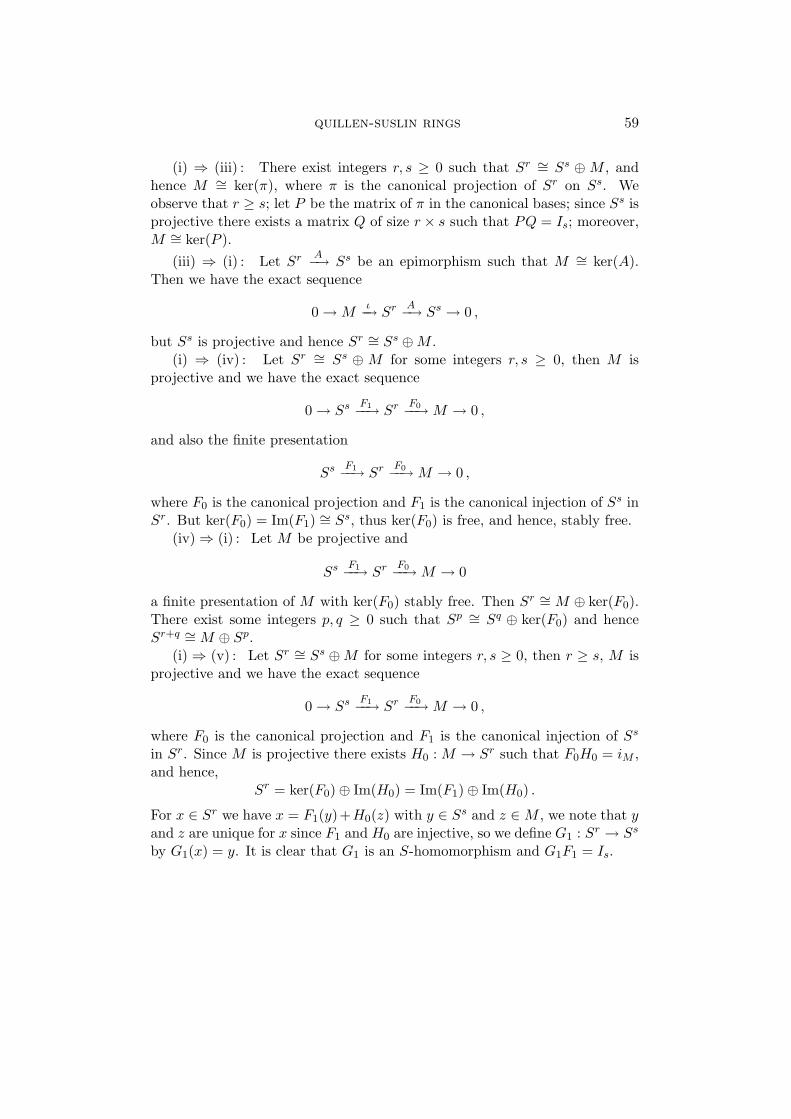
(i) ⇒ (iii) : There exist integers r, s ≥ 0 such that Sr ∼= Ss ⊕ M , andhence M ∼= ker(π), where π is the canonical projection of Sr on Ss. Weobserve that r ≥ s; let P be the matrix of π in the canonical bases; since Ss isprojective there exists a matrix Q of size r × s such that PQ = Is; moreover,M ∼= ker(P ).
(iii) ⇒ (i) : Let Sr A−→ Ss be an epimorphism such that M ∼= ker(A).Then we have the exact sequence
0 → Mι−→ Sr A−→ Ss → 0 ,
but Ss is projective and hence Sr ∼= Ss ⊕M .(i) ⇒ (iv) : Let Sr ∼= Ss ⊕ M for some integers r, s ≥ 0, then M is
projective and we have the exact sequence
0 → Ss F1−−→ Sr F0−−→ M → 0 ,
and also the finite presentation
Ss F1−−→ Sr F0−−→ M → 0 ,
where F0 is the canonical projection and F1 is the canonical injection of Ss inSr. But ker(F0) = Im(F1) ∼= Ss, thus ker(F0) is free, and hence, stably free.
(iv) ⇒ (i) : Let M be projective and
Ss F1−−→ Sr F0−−→ M → 0
a finite presentation of M with ker(F0) stably free. Then Sr ∼= M ⊕ ker(F0).There exist some integers p, q ≥ 0 such that Sp ∼= Sq ⊕ ker(F0) and henceSr+q ∼= M ⊕ Sp.
(i) ⇒ (v) : Let Sr ∼= Ss ⊕M for some integers r, s ≥ 0, then r ≥ s, M isprojective and we have the exact sequence
0 → Ss F1−−→ Sr F0−−→ M → 0 ,
where F0 is the canonical projection and F1 is the canonical injection of Ss
in Sr. Since M is projective there exists H0 : M → Sr such that F0H0 = iM ,and hence,
Sr = ker(F0)⊕ Im(H0) = Im(F1)⊕ Im(H0) .
For x ∈ Sr we have x = F1(y)+H0(z) with y ∈ Ss and z ∈ M , we note that yand z are unique for x since F1 and H0 are injective, so we define G1 : Sr → Ss
by G1(x) = y. It is clear that G1 is an S-homomorphism and G1F1 = Is.
60 o. lezama et al.
(v) ⇒ (i) : Let G1 : Sr → Ss such that G1F1 = Is, then F1 is injectiveand M has the finite free resolution
0 → Ss F1−−→ Sr F0−−→ M → 0 .
By (ii) and (i) M is stably free.(v) ⇔ (vi) : This is a direct consequence of Proposition 5.
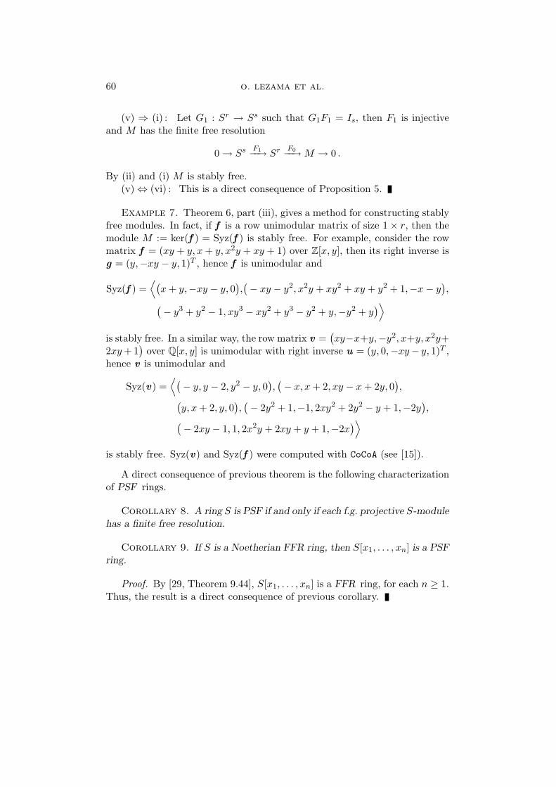
Example 7. Theorem 6, part (iii), gives a method for constructing stablyfree modules. In fact, if f is a row unimodular matrix of size 1× r, then themodule M := ker(f ) = Syz(f ) is stably free. For example, consider the rowmatrix f = (xy + y, x + y, x2y + xy + 1) over Z[x, y], then its right inverse isg = (y,−xy − y, 1)T , hence f is unimodular and
Syz(f ) =⟨(
x + y,−xy − y, 0),(− xy − y2, x2y + xy2 + xy + y2 + 1,−x− y
),
(− y3 + y2 − 1, xy3 − xy2 + y3 − y2 + y,−y2 + y)⟩
is stably free. In a similar way, the row matrix v =(xy−x+y,−y2, x+y, x2y+
2xy + 1)
over Q[x, y] is unimodular with right inverse u = (y, 0,−xy− y, 1)T ,hence v is unimodular and
Syz(v) =⟨(− y, y − 2, y2 − y, 0
),(− x, x + 2, xy − x + 2y, 0
),
(y, x + 2, y, 0
),(− 2y2 + 1,−1, 2xy2 + 2y2 − y + 1,−2y
),
(− 2xy − 1, 1, 2x2y + 2xy + y + 1,−2x)⟩
is stably free. Syz(v) and Syz(f ) were computed with CoCoA (see [15]).
A direct consequence of previous theorem is the following characterizationof PSF rings.
Corollary 8. A ring S is PSF if and only if each f.g. projective S-modulehas a finite free resolution.
Corollary 9. If S is a Noetherian FFR ring, then S[x1, . . . , xn] is a PSFring.
Proof. By [29, Theorem 9.44], S[x1, . . . , xn] is a FFR ring, for each n ≥ 1.Thus, the result is a direct consequence of previous corollary.
quillen-suslin rings 61
Corollary 10. (Serre’s theorem) If K is a field, then for each n ≥ 1,K[x1, . . . , xn] is PSF.
Proof. In [1, Theorem 3.10.4], there is a constructive proof (using Grobnerbases) of Hilbert’s Syzygy theorem that says that K[x1, . . . , xn] is FFR. Thus,Serre’s theorem is a direct consequence of previous corollary.
Matrix descriptions of H rings are presented in the following theorem(compare with [6], [18] and [24]).
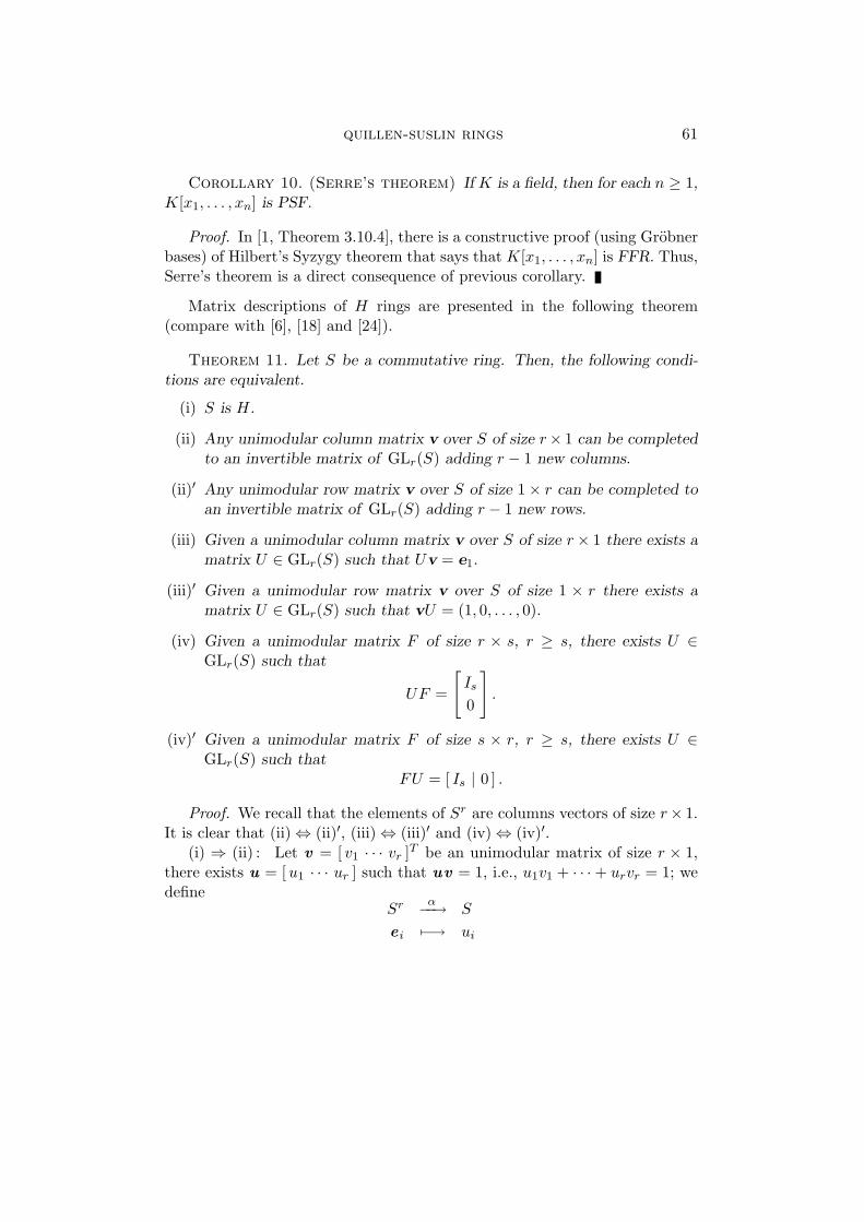
Theorem 11. Let S be a commutative ring. Then, the following condi-tions are equivalent.
(i) S is H.
(ii) Any unimodular column matrix v over S of size r× 1 can be completedto an invertible matrix of GLr(S) adding r − 1 new columns.
(ii)′ Any unimodular row matrix v over S of size 1× r can be completed toan invertible matrix of GLr(S) adding r − 1 new rows.
(iii) Given a unimodular column matrix v over S of size r× 1 there exists amatrix U ∈ GLr(S) such that Uv = e1.
(iii)′ Given a unimodular row matrix v over S of size 1 × r there exists amatrix U ∈ GLr(S) such that vU = (1, 0, . . . , 0).
(iv) Given a unimodular matrix F of size r × s, r ≥ s, there exists U ∈GLr(S) such that
UF =
[Is
0
].
(iv)′ Given a unimodular matrix F of size s × r, r ≥ s, there exists U ∈GLr(S) such that
FU = [ Is | 0 ] .
Proof. We recall that the elements of Sr are columns vectors of size r× 1.It is clear that (ii) ⇔ (ii)′, (iii) ⇔ (iii)′ and (iv) ⇔ (iv)′.
(i) ⇒ (ii) : Let v = [ v1 · · · vr ]T be an unimodular matrix of size r × 1,there exists u = [u1 · · · ur ] such that uv = 1, i.e., u1v1 + · · ·+ urvr = 1; wedefine
Sr α−−→ S
e i 7−→ ui
62 o. lezama et al.
where {e1, . . . , er} is the canonical basis of Sr. We observe that α is a sur-jective homomorphism since α(v) = 1. There exists β : S → Sr such thatαβ = iS and Sr = Im(β)⊕ ker(α); in fact, we define β(1) := v and β is injec-tive, so Im(β) ∼= S is free with basis {v}. This implies that Sr ∼= S ⊕ ker(α),i.e., ker(α) is stably free, so by hypothesis, ker(α) is free of dimension r − 1;let {x 1, . . . ,x r−1} be a basis of ker(α), then {v ,x 1, . . . ,x r−1} is a basis of Sr.This means that [ v x 1 · · · x r−1 ] ∈ GLr(S).
(ii) ⇒ (i) : Let M be an stably free S-module, then there exist integersr, s ≥ 0 such that Sr ∼= Ss ⊕ M . It is enough to prove that M is free forthe case when s = 1. In fact, Ss ⊕ M = S ⊕ (Ss−1 ⊕ M) is free and henceSs−1 ⊕M is free; repeating this reasoning we conclude that S ⊕M is free, soM is free.
Let r ≥ 1 such that Sr ∼= S⊕M , let π : Sr → S be the canonical projectionwith kernel isomorphic to M and let {e1, . . . , er} be the canonical basis ofSr; there exists µ : S → Sr such that πµ = iS and Sr = ker(π)⊕ Im(µ). Letµ(1) = v = [ v1 · · · vr ]T ∈ Sr, then π(v) = 1 = v1π(e1) + · · · + vrπ(er), i.e.,v is a unimodular matrix over S of size r × 1, moreover Sr = ker(π) ⊕ 〈v〉.By hypothesis, there exists U ∈ GLr(S) such that Ue1 = v .
Let f : Sr → Sr be the isomorphism defined by U in the canonical basisof Sr, then f(e1) = v and f(e i) = v i, i ≥ 2, where v2, . . . , v r are the otherscolumns of U .
If we prove that f(e i) ∈ ker(π) for each i ≥ 2, then ker(π) is free, andconsequently, M is free. In fact, let f ′ be the restriction of f to 〈e2, . . . , er〉,i.e., f ′ : 〈e2, . . . , er〉 → ker(π). Then f ′ is bijective: of course f ′ is injective;let w be any vector of Sr, then there exists x ∈ Sr such that f(x ) = w , wewrite x = (x1, x2, . . . , xr) = x1e1 + z , with z = x2e2 + · · · + xrer. We havef(x ) = f(x1e1 + z ) = x1f(e1) + f(z ) = x1v + f(z ) = w . In particular,if w ∈ ker(π), then w − f(z ) ∈ ker(π) ∩ 〈v〉 = 0, so w = f(z ) and hencew = f ′(z ), i.e., f ′ is surjective.
In order to conclude the proof we will show that f(e i) ∈ ker(π) for eachi ≥ 2. Since f was defined by U , the idea is to change U in a such way that itsfirst column was v and for the others columns were v i ∈ ker(π), 2 ≤ i ≤ r. Letπ(v i) = ri ∈ S, i ≥ 2 and v ′i = v i−riv ; then adding to column i of U the firstcolumn multiplied by −ri we get a new matrix U such that its first column isagain v and for the others we have π(v ′i) = π(v i)− riπ(v) = ri − ri = 0, i.e.,v ′i ∈ ker(π).
(ii) ⇒ (iii) : v can be completed to an invertible matrix of GLr(S) if andonly if there exists V ∈ GLr(S) such that V e1 = v if and only if e1 = V −1v ;
quillen-suslin rings 63
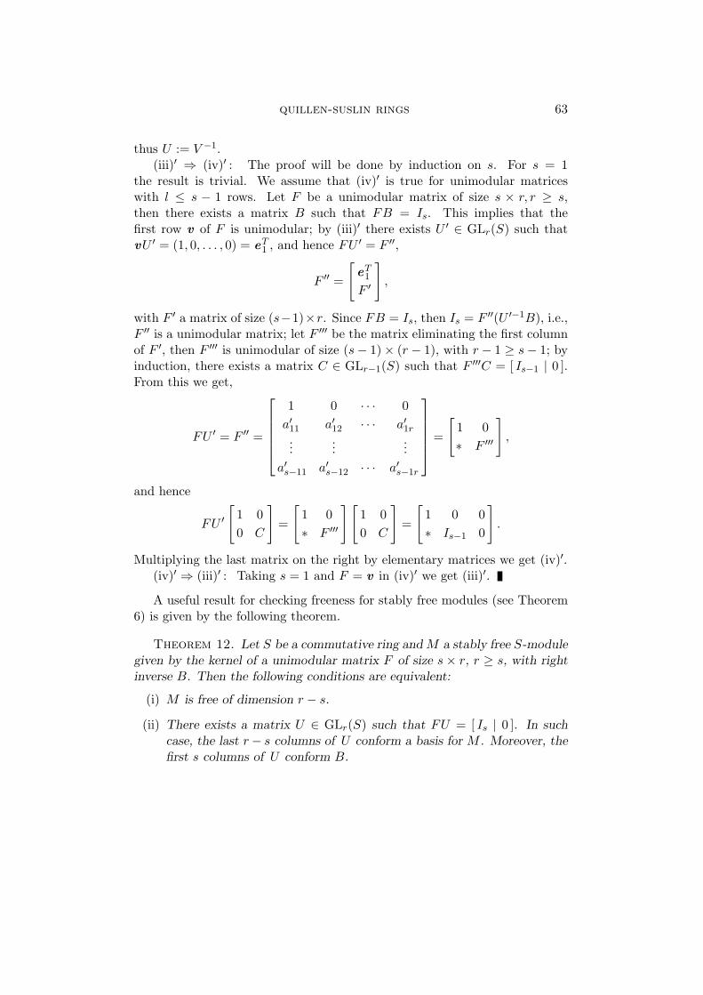
thus U := V −1.(iii)′ ⇒ (iv)′ : The proof will be done by induction on s. For s = 1
the result is trivial. We assume that (iv)′ is true for unimodular matriceswith l ≤ s − 1 rows. Let F be a unimodular matrix of size s × r, r ≥ s,then there exists a matrix B such that FB = Is. This implies that thefirst row v of F is unimodular; by (iii)′ there exists U ′ ∈ GLr(S) such thatvU ′ = (1, 0, . . . , 0) = eT
1 , and hence FU ′ = F ′′,
F ′′ =
[eT
1
F ′
],
with F ′ a matrix of size (s−1)×r. Since FB = Is, then Is = F ′′(U ′−1B), i.e.,F ′′ is a unimodular matrix; let F ′′′ be the matrix eliminating the first columnof F ′, then F ′′′ is unimodular of size (s− 1)× (r − 1), with r − 1 ≥ s− 1; byinduction, there exists a matrix C ∈ GLr−1(S) such that F ′′′C = [ Is−1 | 0 ].From this we get,
FU ′ = F ′′ =
1 0 · · · 0a′11 a′12 · · · a′1r
......
...a′s−11 a′s−12 · · · a′s−1r
=
[1 0∗ F ′′′
],
and hence
FU ′[
1 00 C
]=
[1 0∗ F ′′′
][1 00 C
]=
[1 0 0∗ Is−1 0
].
Multiplying the last matrix on the right by elementary matrices we get (iv)′.(iv)′ ⇒ (iii)′ : Taking s = 1 and F = v in (iv)′ we get (iii)′.
A useful result for checking freeness for stably free modules (see Theorem6) is given by the following theorem.
Theorem 12. Let S be a commutative ring and M a stably free S-modulegiven by the kernel of a unimodular matrix F of size s× r, r ≥ s, with rightinverse B. Then the following conditions are equivalent:
(i) M is free of dimension r − s.
(ii) There exists a matrix U ∈ GLr(S) such that FU = [ Is | 0 ]. In suchcase, the last r− s columns of U conform a basis for M . Moreover, thefirst s columns of U conform B.
64 o. lezama et al.
(iii) There exists a matrix V ∈ GLr(S) such that F coincides with the first srows of V , i.e., F can be completed to an invertible matrix V of GLr(S).
Proof. (i) ⇒ (ii) : Let B be a matrix of size r × s such that FB = Is,moreover let Sr F−→ Ss, then Sr = Im(B) ⊕ ker(F ), thus, we are assumingthat ker(F ) is free. If s = r then F is invertible and U = F−1 = B and theresult is trivially true. Let r > s and let { v1, . . . , vp} be a basis of ker(F )with p := r− s. If {e1, . . . , es} is the canonical basis of Ss, then {u1, . . . ,us}is basis of Im(B) with u i := Be i, 1 ≤ i ≤ s, thus {v1, . . . , vp,u1, . . . ,us} is a
basis of Sr. We define Sr U−→ Sr by U e i := u i for 1 ≤ i ≤ s, and Ues+j := v j
for 1 ≤ j ≤ p. Clearly U is bijective; moreover, FUe i = Fu i = FBe i = e i
and FUes+j = Av j = 0, i.e., FU = [ Is | 0 ]. Additionally, by the definitionof U we observe that the first s columns of U form the matrix B.
(ii) ⇒ (i) : Let U (k) the k-th column of U , then FU = F [ U (1) · · · U (s) · · ·U (r)] = [ Is | 0 ], so FU (i) = e i, 1 ≤ i ≤ s, FU (s+j) = 0, 1 ≤ j ≤ p withp := r − s. This means that U (s+j) ∈ ker(F ) and hence
⟨U (s+j) : 1 ≤ j ≤
p⟩ ⊆ ker(F ). On the other hand, let c ∈ ker(F ) ⊆ Sr, then F c = 0 and
FUU−1c = 0, thus [ Is | 0 ]U−1c = 0 and hence U−1c ∈ ker([ Is | 0 ]); letd = [d1, . . . , dr]T ∈ ker( Is | 0 ]), then [ Is | 0 ]d = 0 and from this we concludethat d1 = · · · = ds = 0, i.e., ker([ Is | 0 ]) = 〈es+1, es+2, . . . , es+p〉, in otherwords, ker([ Is | 0 ]) coincides with the column module of the matrix
[0Ip
].
From U−1c ∈ ker([ Is | 0 ]) we get that c is in the column module of matrix
U
[0Ip
]=
[U (s+1) · · · U (s+p)
].
This proves that ker(F ) =⟨U (s+j) : 1 ≤ j ≤ p
⟩; but since U is invertible,
then ker(F ) ∼= M is free of dimension p = r− s. We also has proved that thelast r − s columns of U conform a basis for M .
(ii) ⇔ (iii) : FU = [ Is | 0 ] if and only if F = [ Is | 0 ]U−1, but the first srows of [ Is | 0 ]U−1 coincides with the first s rows of U−1; taking V := U−1
we get the result.
Some examples of H rings are presented next.
quillen-suslin rings 65
Example 13. Semilocal rings are H. This can be proved in the followingway: finite product of H rings is a H ring; S is a H ring if and only ifS/Rad(S) is a H ring (Rad(S) is the Jacobson radical of S ); any field is a Hring, so we conclude the proof applying the chinese remainder theorem. Onthe other hand, from (iv) of Example 2 we get that
PF $ H .
Moreover, from Examples 2 and (2.1) we get that semilocals rings are notalways PSF.
Examples 14. (i) If R is a Dedekind domain (hereditary integral do-main), then R[x1, . . . , xn] is H, for any n ≥ 1 (see [18, Theorem V.2.11]).
(ii) If S is a commutative ring of Krull dimension 0, then S[x1, . . . , xn] isH, for any n ≥ 1 (see [18, Proposition V.2.13]).
(iii) If S is a local ring, in [3] Bhatwadekar and Rao have proved that S[x]is H if and only if S〈x〉 is H, where S〈x〉 is the localization of S[x] at themultiplicative set of monic polynomials (see also [18, Theorem 5.9]).
Example 15. Now we will exhibit a ring that is not H (see [6]); thisexample also shows that if S is H not always S/I is H, where I is a properideal of S: let S := R[x, y, z]/I and I := 〈x2 + y2 + z2− 1〉, then f := (x, y, z)is unimodular with right inverse f T , however f cannot be completed to aunimodular matrix.
Related with the H condition there are two well known conjectures (see[18]), probably not solved yet, that could be investigated with the results ofTheorem 11:
Conjectures 16. (i) If S is H, then S[x] is H.(ii) If S is local, then S[x] is H.
3. A constructive proof of the Quillen-Suslin’s theorem
The most famous example of QS ring is given by the Quillen-Suslin the-orem proved not only for coefficients in a field but also for coefficients in aPID :
Let D be a PID, then for n ≥ 1 every finitely generated projectiveD[x1, . . . , xn]-module is free, i.e., D[x1, . . . , xn] is PF.
66 o. lezama et al.
Thus, the Quillen-Suslin theorem stays that any PID is QS. A complete studyof the Quillen-Suslin’s theorem could be found in [18]. A non-algorithmic proofof this key theorem could be found in [28], [31], [17], [18], [19] and [29].
In this section we present a clear and constructive proof of the theoremin the classical case, i.e., when the coefficients are in a field (compare with[24]). More exactly, if M ⊆ (K[x1, . . . , xn])m is a f.g. projective module, Ka field, the procedure that will exhibit in the following two theorems showshow to construct a free basis for M . For this purpose we will adapt theLogar-Sturmfels’ algorithm of [24] and also the ideas in [27].
The first theorem (Theorem 20) proves that K[x1, . . . , xn] is an Hermitering; the second theorem (Theorem 21) constructs a finite free basis for M .In order to prove these two theorems we need some preliminary lemmas.
Lemma 17. (Noether normalization) Let p(x1, . . . , xn) ∈ K[x1,. . . , xn] and m := deg(p(x1, . . . , xn)) + 1, where deg(p(x1, . . . , xn)) is thetotal degree of p(x1, . . . , xn). Consider the following automorphism ofK[x1, . . . , xn]
yn := xn , yi := xi − xmn−i
n , 1 ≤ i ≤ n− 1 .
Then, p(y1, . . . , yn) = aq(yn), where a ∈ K − {0} and q(yn) ∈ R[yn] is monic,with R := K[y1, . . . , yn−1]. In the case where K is an infinite field, the auto-morphism could be taken linear, i.e., yi :=
∑nj=1 mijxj , where M = [mij ] is
an invertible matrix over K.
Proof. See [29, Lemma 4.58] and [13, Theorem 3.4.1].
Lemma 18. Let S be a commutative ring and let f1, f2, b, d ∈ S[x]. Lets := Resx(f1, f2) ∈ S be the resultant of f1 and f2 with respect to x. Then,there exists U ∈ GL2(S[x]) such that
[f1(b) f2(b)
]U =
[f1(b + sd) f2(b + sd)
].
Proof. The proof in [27] of this lemma is constructive and we will include it.For the resultant of two polynomials consult [5] or [19]. Using Grobner baseswe can find p1, p2 ∈ S[x] such that s = f1p1 +f2p2. Let s1, s2, t1, t2 ∈ S[x, y, z]
quillen-suslin rings 67
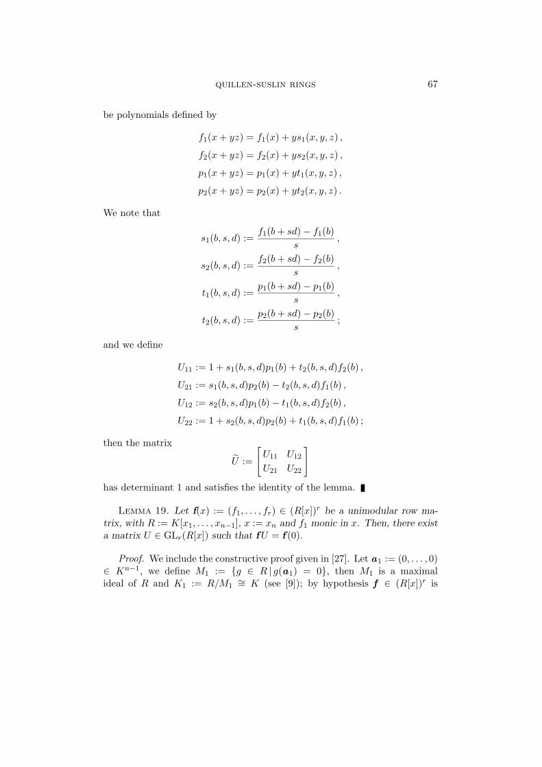
be polynomials defined by
f1(x + yz) = f1(x) + ys1(x, y, z) ,
f2(x + yz) = f2(x) + ys2(x, y, z) ,
p1(x + yz) = p1(x) + yt1(x, y, z) ,
p2(x + yz) = p2(x) + yt2(x, y, z) .
We note that
s1(b, s, d) :=f1(b + sd)− f1(b)
s,
s2(b, s, d) :=f2(b + sd)− f2(b)
s,
t1(b, s, d) :=p1(b + sd)− p1(b)
s,
t2(b, s, d) :=p2(b + sd)− p2(b)
s;
and we define
U11 := 1 + s1(b, s, d)p1(b) + t2(b, s, d)f2(b) ,
U21 := s1(b, s, d)p2(b)− t2(b, s, d)f1(b) ,
U12 := s2(b, s, d)p1(b)− t1(b, s, d)f2(b) ,
U22 := 1 + s2(b, s, d)p2(b) + t1(b, s, d)f1(b) ;
then the matrix
U :=
[U11 U12
U21 U22
]
has determinant 1 and satisfies the identity of the lemma.
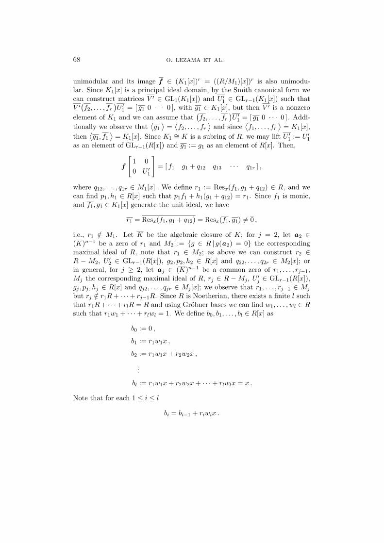
Lemma 19. Let f(x) := (f1, . . . , fr) ∈ (R[x])r be a unimodular row ma-trix, with R := K[x1, . . . , xn−1], x := xn and f1 monic in x. Then, there exista matrix U ∈ GLr(R[x]) such that fU = f (0).
Proof. We include the constructive proof given in [27]. Let a1 := (0, . . . , 0)∈ Kn−1, we define M1 := {g ∈ R | g(a1) = 0}, then M1 is a maximalideal of R and K1 := R/M1
∼= K (see [9]); by hypothesis f ∈ (R[x])r is
68 o. lezama et al.
unimodular and its image f ∈ (K1[x])r = ((R/M1)[x])r is also unimodu-lar. Since K1[x] is a principal ideal domain, by the Smith canonical form wecan construct matrices V ′ ∈ GL1(K1[x]) and U ′
1 ∈ GLr−1(K1[x]) such thatV ′(f2, . . . , fr
)U ′
1 = [ g1 0 · · · 0 ], with g1 ∈ K1[x], but then V ′ is a nonzeroelement of K1 and we can assume that
(f2, . . . , fr
)U ′
1 = [ g1 0 · · · 0 ]. Addi-tionally we observe that
⟨g1
⟩=
⟨f2, . . . , fr
⟩and since
⟨f1, . . . , fr
⟩= K1[x],
then⟨g1, f1
⟩= K1[x]. Since K1
∼= K is a subring of R, we may lift U ′1 := U ′
1
as an element of GLr−1(R[x]) and g1 := g1 as an element of R[x]. Then,
f
[1 00 U ′
1
]= [ f1 g1 + q12 q13 · · · q1r ] ,
where q12, . . . , q1r ∈ M1[x]. We define r1 := Resx(f1, g1 + q12) ∈ R, and wecan find p1, h1 ∈ R[x] such that p1f1 + h1(g1 + q12) = r1. Since f1 is monic,and f1, g1 ∈ K1[x] generate the unit ideal, we have
r1 = Resx(f1, g1 + q12) = Resx(f1, g1) 6= 0 ,
i.e., r1 /∈ M1. Let K be the algebraic closure of K; for j = 2, let a2 ∈(K)n−1 be a zero of r1 and M2 := {g ∈ R | g(a2) = 0} the correspondingmaximal ideal of R, note that r1 ∈ M2; as above we can construct r2 ∈R − M2, U ′
2 ∈ GLr−1(R[x]), g2, p2, h2 ∈ R[x] and q22, . . . , q2r ∈ M2[x]; orin general, for j ≥ 2, let a j ∈ (K)n−1 be a common zero of r1, . . . , rj−1,Mj the corresponding maximal ideal of R, rj ∈ R −Mj , U ′
j ∈ GLr−1(R[x]),gj , pj , hj ∈ R[x] and qj2, . . . , qjr ∈ Mj [x]; we observe that r1, . . . , rj−1 ∈ Mj
but rj /∈ r1R + · · ·+ rj−1R. Since R is Noetherian, there exists a finite l suchthat r1R + · · ·+ rlR = R and using Grobner bases we can find w1, . . . , wl ∈ Rsuch that r1w1 + · · ·+ rlwl = 1. We define b0, b1, . . . , bl ∈ R[x] as
b0 := 0 ,
b1 := r1w1x ,
b2 := r1w1x + r2w2x ,
...
bl := r1w1x + r2w2x + · · ·+ rlwlx = x .
Note that for each 1 ≤ i ≤ l
bi = bi−1 + riwix .
quillen-suslin rings 69
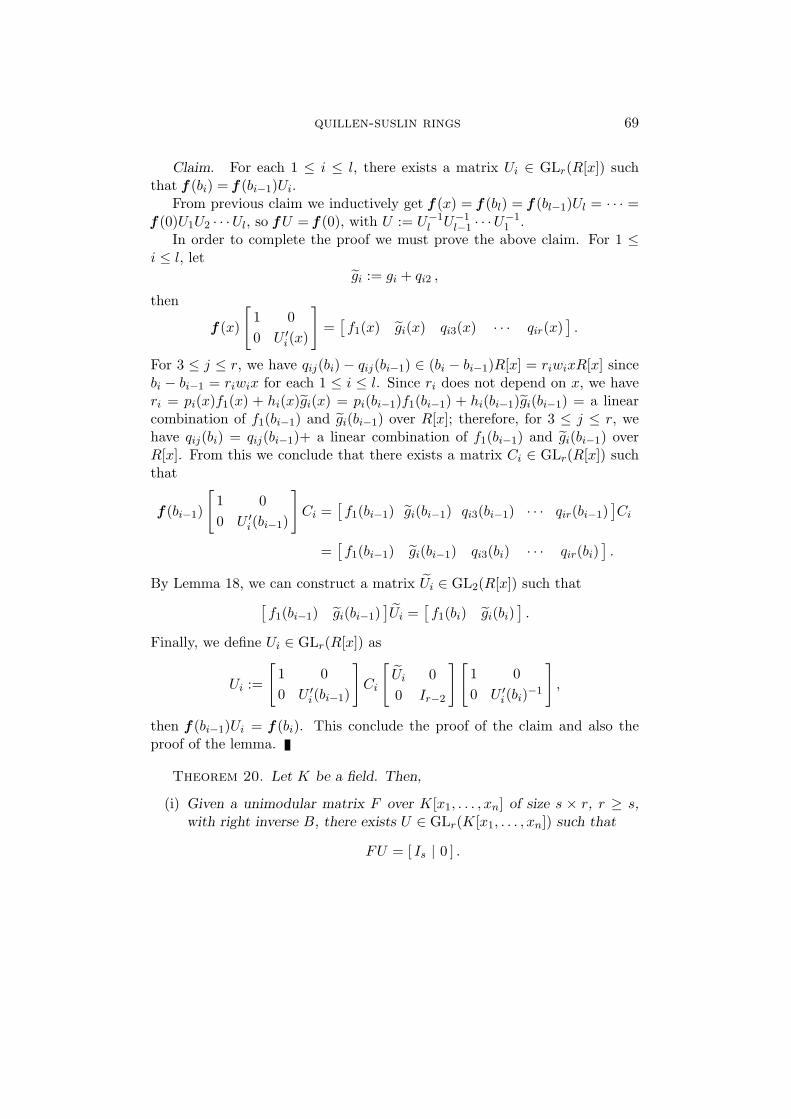
Claim. For each 1 ≤ i ≤ l, there exists a matrix Ui ∈ GLr(R[x]) suchthat f (bi) = f (bi−1)Ui.
From previous claim we inductively get f (x) = f (bl) = f (bl−1)Ul = · · · =f (0)U1U2 · · ·Ul, so f U = f (0), with U := U−1
l U−1l−1 · · ·U−1
1 .In order to complete the proof we must prove the above claim. For 1 ≤
i ≤ l, letgi := gi + qi2 ,
then
f (x)
[1 00 U ′
i(x)
]=
[f1(x) gi(x) qi3(x) · · · qir(x)
].
For 3 ≤ j ≤ r, we have qij(bi)− qij(bi−1) ∈ (bi − bi−1)R[x] = riwixR[x] sincebi − bi−1 = riwix for each 1 ≤ i ≤ l. Since ri does not depend on x, we haveri = pi(x)f1(x) + hi(x)gi(x) = pi(bi−1)f1(bi−1) + hi(bi−1)gi(bi−1) = a linearcombination of f1(bi−1) and gi(bi−1) over R[x]; therefore, for 3 ≤ j ≤ r, wehave qij(bi) = qij(bi−1)+ a linear combination of f1(bi−1) and gi(bi−1) overR[x]. From this we conclude that there exists a matrix Ci ∈ GLr(R[x]) suchthat
f (bi−1)
[1 00 U ′
i(bi−1)
]Ci =
[f1(bi−1) gi(bi−1) qi3(bi−1) · · · qir(bi−1)
]Ci
=[f1(bi−1) gi(bi−1) qi3(bi) · · · qir(bi)
].
By Lemma 18, we can construct a matrix Ui ∈ GL2(R[x]) such that[f1(bi−1) gi(bi−1)
]Ui =
[f1(bi) gi(bi)
].
Finally, we define Ui ∈ GLr(R[x]) as
Ui :=
[1 00 U ′
i(bi−1)
]Ci
[Ui 00 Ir−2
][1 00 U ′
i(bi)−1
],
then f (bi−1)Ui = f (bi). This conclude the proof of the claim and also theproof of the lemma.
Theorem 20. Let K be a field. Then,
(i) Given a unimodular matrix F over K[x1, . . . , xn] of size s × r, r ≥ s,with right inverse B, there exists U ∈ GLr(K[x1, . . . , xn]) such that
FU = [ Is | 0 ] .
70 o. lezama et al.
In such case, the last r − s columns of U conform a basis for ker(F ).Moreover, the first s columns of U conform B.
(ii) Given a unimodular matrix F over K[x1, . . . , xn] of size r × s, r ≥ s,with left inverse B, there exists U ∈ GLr(K[x1, . . . , xn]) such that
UF = [ Is | 0 ] .
In such case, the last r− s rows of U conform a basis for ker(F ). More-over, the first s rows of U conform B.
Proof. Taking the transposes of matrices involved we observe that (i) and(ii) are equivalent, so we only need to prove (i). The second part of (i) wasproven in Theorem 12. Moreover, by induction, we only need to consider thecase s = 1 (see also the proof of Theorem 11).
Thus, given a unimodular row matrix f = (f1, . . . , fr) over K[x1, . . . , xn]of size 1 × r we will construct a matrix U ∈ GLr(K[x1, . . . , xn]) such thatf U = (1, 0 . . . , 0).
Case 1. For r = 1 the property is trivially true. For r = 2 the propertyis valid for any commutative ring R: in fact, let g = (g1, g2) ∈ R2 such thatf gT = [1], i.e., f1g1 + f2g2 = 1, then in this case the matrix U is
U :=
[g1 −f2
g2 f1
]
since det(U) = 1 and f U = (1, 0).Case 2. We can assume that r ≥ 3. For n = 1 the matrix U is computable
since K[x1] is a principal ideal domain: in fact, by the Smith canonical formwe can construct matrices V ∈ GL1(K[x1]) and U ∈ GLr(K[x1]) such thatV f U = [ d 0 · · · 0 ], with d ∈ K[x1], but then V is a nonzero elementof K and we can assume that f U = [ d 0 · · · 0 ]. Since U is invertible〈d〉 = 〈f1, . . . , fr〉 = K[x1] and hence d is a nonzero constant of K, so we canassume that d = 1 and f U = [ 1 0 · · · 0 ].
The rest of the proof is as in [27]. We assume that the result is true fork ≤ n−1 variables and let R := K[x1, . . . , xn−1] and x := xn; let f (x) := f =(f1, . . . , fr) ∈ K[x1, . . . , xn] = R[x] be a unimodular row matrix. Permutingsome columns of f (if it is necessary) and by Lemma 17 we can assume thatf1 is monic. By Lemma 19 we can construct a matrix U ′ ∈ GLr(R[x]) suchthat
f U ′ = f (0) ∈ R .
quillen-suslin rings 71
Since f (0) is unimodular over R, by induction there exists a matrix U ′′ ∈GLr(R) such that f (0)U ′′ = (1, 0, . . . , 0), and then, f U = (1, 0, . . . , 0), withU := U ′U ′′ ∈ GLr(R[x]).
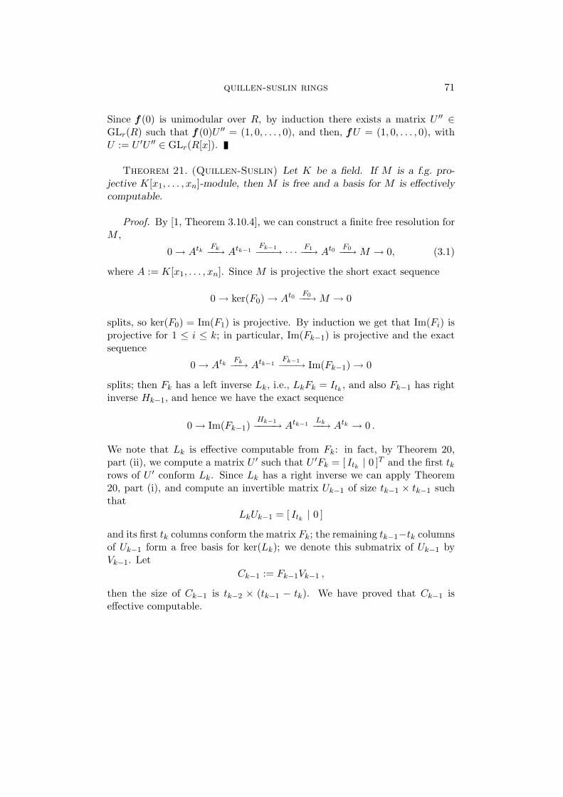
Theorem 21. (Quillen-Suslin) Let K be a field. If M is a f.g. pro-jective K[x1, . . . , xn]-module, then M is free and a basis for M is effectivelycomputable.
Proof. By [1, Theorem 3.10.4], we can construct a finite free resolution forM ,
0 → Atk Fk−−→ Atk−1Fk−1−−−→ · · · F1−−→ At0 F0−−→ M → 0, (3.1)
where A := K[x1, . . . , xn]. Since M is projective the short exact sequence
0 → ker(F0) → At0 F0−−→ M → 0
splits, so ker(F0) = Im(F1) is projective. By induction we get that Im(Fi) isprojective for 1 ≤ i ≤ k; in particular, Im(Fk−1) is projective and the exactsequence
0 → Atk Fk−−→ Atk−1Fk−1−−−→ Im(Fk−1) → 0
splits; then Fk has a left inverse Lk, i.e., LkFk = Itk , and also Fk−1 has rightinverse Hk−1, and hence we have the exact sequence
0 → Im(Fk−1)Hk−1−−−−→ Atk−1
Lk−−→ Atk → 0 .
We note that Lk is effective computable from Fk: in fact, by Theorem 20,part (ii), we compute a matrix U ′ such that U ′Fk = [ Itk | 0 ]T and the first tkrows of U ′ conform Lk. Since Lk has a right inverse we can apply Theorem20, part (i), and compute an invertible matrix Uk−1 of size tk−1 × tk−1 suchthat
LkUk−1 = [ Itk | 0 ]
and its first tk columns conform the matrix Fk; the remaining tk−1−tk columnsof Uk−1 form a free basis for ker(Lk); we denote this submatrix of Uk−1 byVk−1. Let
Ck−1 := Fk−1Vk−1 ,
then the size of Ck−1 is tk−2 × (tk−1 − tk). We have proved that Ck−1 iseffective computable.
72 o. lezama et al.
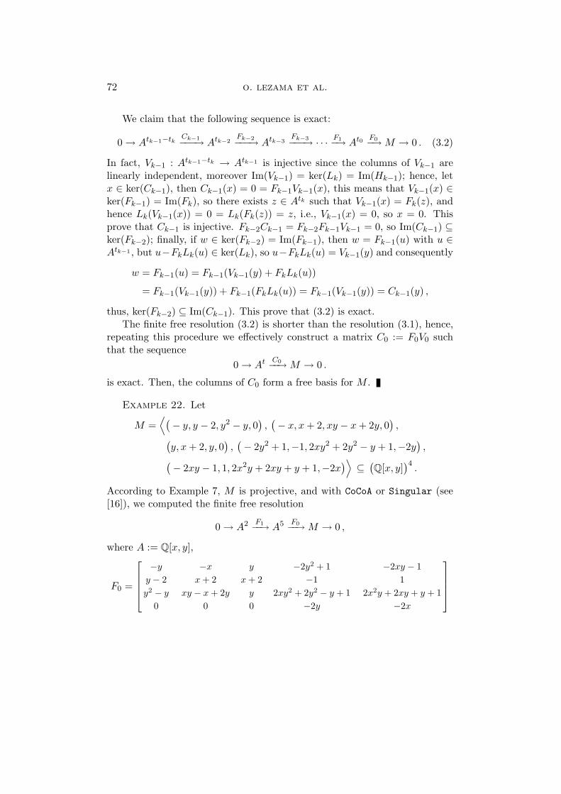
We claim that the following sequence is exact:
0 → Atk−1−tkCk−1−−−→ Atk−2
Fk−2−−−→ Atk−3Fk−3−−−→ · · · F1−→ At0 F0−→ M → 0 . (3.2)
In fact, Vk−1 : Atk−1−tk → Atk−1 is injective since the columns of Vk−1 arelinearly independent, moreover Im(Vk−1) = ker(Lk) = Im(Hk−1); hence, letx ∈ ker(Ck−1), then Ck−1(x) = 0 = Fk−1Vk−1(x), this means that Vk−1(x) ∈ker(Fk−1) = Im(Fk), so there exists z ∈ Atk such that Vk−1(x) = Fk(z), andhence Lk(Vk−1(x)) = 0 = Lk(Fk(z)) = z, i.e., Vk−1(x) = 0, so x = 0. Thisprove that Ck−1 is injective. Fk−2Ck−1 = Fk−2Fk−1Vk−1 = 0, so Im(Ck−1) ⊆ker(Fk−2); finally, if w ∈ ker(Fk−2) = Im(Fk−1), then w = Fk−1(u) with u ∈Atk−1 , but u−FkLk(u) ∈ ker(Lk), so u−FkLk(u) = Vk−1(y) and consequently
w = Fk−1(u) = Fk−1(Vk−1(y) + FkLk(u))
= Fk−1(Vk−1(y)) + Fk−1(FkLk(u)) = Fk−1(Vk−1(y)) = Ck−1(y) ,
thus, ker(Fk−2) ⊆ Im(Ck−1). This prove that (3.2) is exact.The finite free resolution (3.2) is shorter than the resolution (3.1), hence,
repeating this procedure we effectively construct a matrix C0 := F0V0 suchthat the sequence
0 → At C0−−→ M → 0 .
is exact. Then, the columns of C0 form a free basis for M .
Example 22. Let
M =⟨(− y, y − 2, y2 − y, 0
),(− x, x + 2, xy − x + 2y, 0
),
(y, x + 2, y, 0
),(− 2y2 + 1,−1, 2xy2 + 2y2 − y + 1,−2y
),
(− 2xy − 1, 1, 2x2y + 2xy + y + 1,−2x)⟩ ⊆ (
Q[x, y])4
.
According to Example 7, M is projective, and with CoCoA or Singular (see[16]), we computed the finite free resolution
0 → A2 F1−−→ A5 F0−−→ M → 0 ,
where A := Q[x, y],
F0 =
−y −x y −2y2 + 1 −2xy − 1y − 2 x + 2 x + 2 −1 1y2 − y xy − x + 2y y 2xy2 + 2y2 − y + 1 2x2y + 2xy + y + 1
0 0 0 −2y −2x
quillen-suslin rings 73
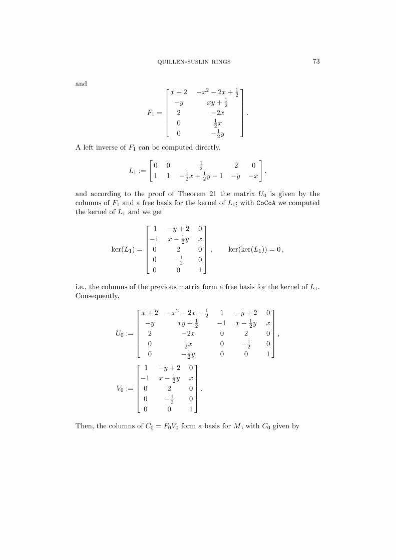
and
F1 =
x + 2 −x2 − 2x + 12
−y xy + 12
2 −2x
0 12x
0 −12y
.
A left inverse of F1 can be computed directly,
L1 :=
[0 0 1
2 2 01 1 −1
2x + 12y − 1 −y −x
],
and according to the proof of Theorem 21 the matrix U0 is given by thecolumns of F1 and a free basis for the kernel of L1; with CoCoA we computedthe kernel of L1 and we get
ker(L1) =
1 −y + 2 0−1 x− 1
2y x
0 2 00 −1
2 00 0 1
, ker(ker(L1)) = 0 ,
i.e., the columns of the previous matrix form a free basis for the kernel of L1.Consequently,
U0 :=
x + 2 −x2 − 2x + 12 1 −y + 2 0
−y xy + 12 −1 x− 1
2y x
2 −2x 0 2 00 1
2x 0 −12 0
0 −12y 0 0 1
,
V0 :=
1 −y + 2 0−1 x− 1
2y x
0 2 00 −1
2 00 0 1
.
Then, the columns of C0 = F0V0 form a basis for M , with C0 given by
74 o. lezama et al.
C0 =
x− y −x2 + 12xy + 2y2 − 1
2 −x2 − 2yx− 1y − x− 4 x2 − 1
2xy + 4x− y2 + 3y + 12 x2 + 2x + 1
α β γ
0 y −2x
,
where
α = x− 3y − xy + y2 ,
β = x2y − x2 − 32xy2 +
52xy − y3 + y2 +
12y − 1
2,
γ = y + 3x2y + 4xy − x2 + 1 .
With CoCoA we checked that ker(C0) = 0 and M coincides with the columnmodule of C0:
UseR ::= Q[x, y];
Syz([V ector(x− y, y − x− 4, x− 3y − xy + y2, 0),
V ector(−x2 + 1/2xy + 2y2 − 1/2, x2 − 1/2xy + 4x− y2 + 3y + 1/2,
x2y − x2 − 3/2xy2 + 5/2xy − y3 + y2 + 1/2y − 1/2, y),
V ector(−x2 − 2yx− 1, x2 + 2x + 1, y + 3x2y + 4xy − x2 + 1,−2x)]);
Module([0])
UseR ::= Q[x, y];
G := ReducedGBasis(Module(V ector(x− y, y − x− 4, x− 3y − xy + y2, 0),
V ector(−x2 + 1/2xy + 2y2 − 1/2, x2 − 1/2xy + 4x− y2 + 3y + 1/2,
x2y − x2 − 3/2xy2 + 5/2xy − y3 + y2 + 1/2y − 1/2, y),
V ector(−x2 − 2yx− 1, x2 + 2x + 1, y + 3x2y + 4xy − x2 + 1,−2x)));
G;
[V ector(y, x + 2, y, 0), V ector(−x− y, 0, xy − x + y, 0),
V ector(x2 − 1/2, 1/2, x2 + 1/2y + 1/2,−x), V ector(−y, y − 2, y2 − y, 0),
V ector(xy + x + y + 1/2,−1/2, x− 3/2y + 1/2,−y)]
quillen-suslin rings 75
UseR ::= Q[x, y];
G := ReducedGBasis(Module(V ector(−y, y − 2, y2 − y, 0),
V ector(−x, x + 2, xy − x + 2y, 0),
V ector(y, x + 2, y, 0), V ector(−2y2 + 1,−1, 2xy2 + 2y2 − y + 1,−2y),
V ector(−2xy − 1, 1, 2x2y + 2xy + y + 1,−2x)));
G;
[V ector(−y, y − 2, y2 − y, 0),
V ector(xy + x + y + 1/2,−1/2, x− 3/2y + 1/2,−y),
V ector(x2 − 1/2, 1/2, x2 + 1/2y + 1/2,−x), V ector(y, x + 2, y, 0),
V ector(−x− y, 0, xy − x + y, 0)]
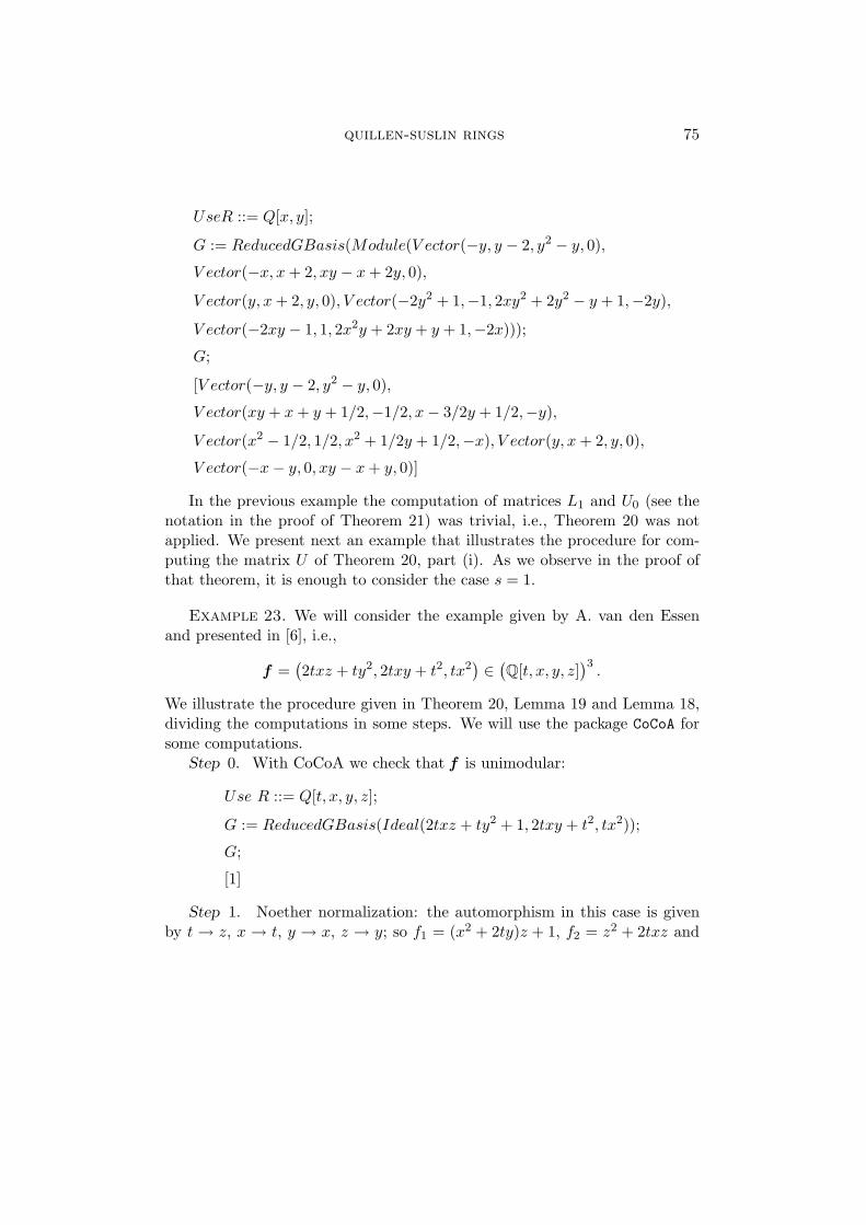
In the previous example the computation of matrices L1 and U0 (see thenotation in the proof of Theorem 21) was trivial, i.e., Theorem 20 was notapplied. We present next an example that illustrates the procedure for com-puting the matrix U of Theorem 20, part (i). As we observe in the proof ofthat theorem, it is enough to consider the case s = 1.
Example 23. We will consider the example given by A. van den Essenand presented in [6], i.e.,
f =(2txz + ty2, 2txy + t2, tx2
) ∈ (Q[t, x, y, z]
)3.
We illustrate the procedure given in Theorem 20, Lemma 19 and Lemma 18,dividing the computations in some steps. We will use the package CoCoA forsome computations.
Step 0. With CoCoA we check that f is unimodular:
Use R ::= Q[t, x, y, z];
G := ReducedGBasis(Ideal(2txz + ty2 + 1, 2txy + t2, tx2));
G;
[1]
Step 1. Noether normalization: the automorphism in this case is givenby t → z, x → t, y → x, z → y; so f1 = (x2 + 2ty)z + 1, f2 = z2 + 2txz and
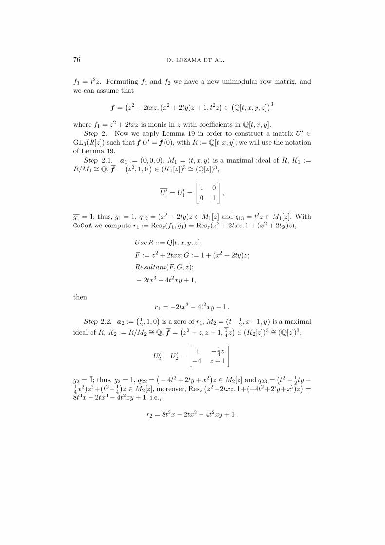
76 o. lezama et al.
f3 = t2z. Permuting f1 and f2 we have a new unimodular row matrix, andwe can assume that
f =(z2 + 2txz, (x2 + 2ty)z + 1, t2z
) ∈ (Q[t, x, y, z]
)3
where f1 = z2 + 2txz is monic in z with coefficients in Q[t, x, y].Step 2. Now we apply Lemma 19 in order to construct a matrix U ′ ∈
GL3(R[z]) such that f U ′ = f (0), with R := Q[t, x, y]; we will use the notationof Lemma 19.
Step 2.1. a1 := (0, 0, 0), M1 = 〈t, x, y〉 is a maximal ideal of R, K1 :=R/M1
∼= Q, f =(z2, 1, 0
) ∈ (K1[z])3 ∼= (Q[z])3,
U ′1 = U ′
1 =
[1 00 1
],
g1 = 1; thus, g1 = 1, q12 = (x2 + 2ty)z ∈ M1[z] and q13 = t2z ∈ M1[z]. WithCoCoA we compute r1 := Resz(f1, g1) = Resz(z2 + 2txz, 1 + (x2 + 2ty)z),
Use R ::= Q[t, x, y, z];
F := z2 + 2txz; G := 1 + (x2 + 2ty)z;
Resultant(F,G, z);
− 2tx3 − 4t2xy + 1,
thenr1 = −2tx3 − 4t2xy + 1 .
Step 2.2. a2 :=(
12 , 1, 0
)is a zero of r1, M2 =
⟨t− 1
2 , x−1, y⟩
is a maximalideal of R, K2 := R/M2
∼= Q, f =(z2 + z, z + 1, 1
4z) ∈ (K2[z])3 ∼= (Q[z])3,
U ′2 = U ′
2 =
[1 −1
4z
−4 z + 1
]
g2 = 1; thus, g2 = 1, q22 =(− 4t2 + 2ty + x2
)z ∈ M2[z] and q23 =
(t2− 1
2 ty−14x2)z2+(t2− 1
4
)z ∈ M2[z], moreover, Resz
(z2+2txz, 1+(−4t2+2ty+x2)z
)=
8t3x− 2tx3 − 4t2xy + 1, i.e.,
r2 = 8t3x− 2tx3 − 4t2xy + 1 .
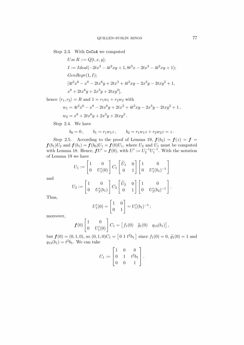
quillen-suslin rings 77
Step 2.3. With CoCoA we computed
Use R ::= Q[t, x, y];
I := Ideal(−2tx3 − 4t2xy + 1, 8t3x− 2tx3 − 4t2xy + 1);
GenRepr(1, I);
[4t2x6 − x8 − 2tx6y + 2tx3 + 4t2xy − 2x3y − 2txy2 + 1,
x8 + 2tx6y + 2x3y + 2txy2],
hence 〈r1, r2〉 = R and 1 = r1w1 + r2w2 with
w1 = 4t2x6 − x8 − 2tx6y + 2tx3 + 4t2xy − 2x3y − 2txy2 + 1 ,
w2 = x8 + 2tx6y + 2x3y + 2txy2 .
Step 2.4. We have
b0 = 0 , b1 = r1w1z , b2 = r1w1z + r2w2z = z .
Step 2.5. According to the proof of Lemma 19, f (b2) = f (z) = f =f (b1)U2 and f (b1) = f (b0)U1 = f (0)U1, where U2 and U1 must be computedwith Lemma 18. Hence, f U ′ = f (0), with U ′ := U−1
2 U−11 . With the notation
of Lemma 19 we have
U1 :=
[1 00 U ′
1(0)
]C1
[U1 00 1
][1 00 U ′
1(b1)−1
]
and
U2 :=
[1 00 U ′
2(b1)
]C2
[U2 00 1
][1 00 U ′
2(b2)−1
].
Thus,
U ′1(0) =
[1 00 1
]= U ′
1(b1)−1 ;
moreover,
f (0)
[1 00 U ′
1(0)
]C1 =
[f1(0) g1(0) q13(b1)
],
but f (0) = (0, 1, 0), so (0, 1, 0)C1 =[0 1 t2b1
]since f1(0) = 0, g1(0) = 1 and
q13(b1) = t2b1. We can take
C1 :=
1 0 00 1 t2b1
0 0 1
.
78 o. lezama et al.
Moreover, for U1 we have[f1(0) g1(0)
]=
[f1(b1) g1(b1)
],
Lemma 18 gives a procedure for computing U1, let
U1 =
[u11 u12
u21 u22
];
using the proof of Lemma 18 with b = b0 = 0, s = r1, d = w1z, we have
u11 = 1 + s1(0, r1, w1z)p1(0) + t2(0, r1, w1z)g1(0) ,
u21 = s1(0, r1, w1z)h1(0)− t2(0, r1, w1z)f1(0) ,
u12 = s2(0, r1, w1z)p1(0)− t1(0, r1, w1z)g1(0) ,
u22 = 1 + s2(0, r1, w1z)h1(0) + t1(0, r1, w1z)f1(0) ,
where p1f1 + h1(g1 + q12) = r1 and p1, h1, s1, s2, t1, t2 are some polynomialsthat we must compute. With CoCoA we computed
p1 = x4 + 4tx2y + 4t2y2
h1 = −2tx3 − 4t2xy − x2z − 2tyz + 1 .
Since g1(0) = 1, f1(0) = 0, p1(0) = p1 and h1(0) = r1, by Lemma 18
s1 =f1(b1)− f1(b0)
r1= w1z(r1w1z + 2tx) ,
s2 =g1(b1)− g1(b0)
r1= w1z(x2 + 2ty) ,
t1 =p1(b1)− p1(b0)
r1= 0 ,
t2 =h1(b1)− h1(b0)
r1= −w1z(x2 + 2ty) .
From all of these computations we conclude that
u11 = 1 + w1z(r1w1z + 2tx)(x2 + 2ty)2 − w1z(x2 + 2ty) ,
u21 = r1w1z(r1w1z + 2tx) ,
u12 = w1z(x2 + 2ty)3 ,
u22 = 1 + r1w1z(x2 + 2ty) ,
quillen-suslin rings 79
and
U1 =
u11 u12 0u21 u22 t2b1
0 0 1
;
we observe that det(U1) = 1 and
U−11 =
u22 −u12 u12t2b1
−u21 u11 −u11t2b1
0 0 1
.
Now we will compute U−12 . We start with C2, we have
[f1(b1) g2(b1) q23(b1)
]C2 =
[f1(b1) g2(b1) q23(b2)
];
since q23(b2) = q23(b1)+ a linear combination of f1(b1) and g2(b1) over R[z],we conclude that the form of C2 is
C2 =
1 0 p
0 1 q
0 0 1
,
where p, q are polynomials that we must compute; we get that
q23(b2) = pf1(b1) + qg2(b1) + q23(b1) .
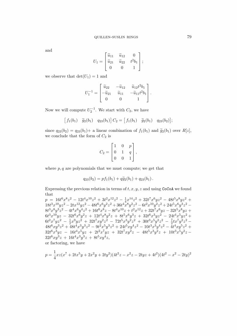
Expressing the previous relation in terms of t, x, y, z and using CoCoA we foundthatp = 16t6x8z2 − 12t4x10z2 + 3t2x12z2 − 1
4x14z2 + 32t7x6yz2 − 48t5x8yz2 +18t3x10yz2− 2tx12yz2− 48t6x6y2z2 + 36t4x8y2z2− 6t2x10y2z2 + 24t5x6y3z2−8t3x8y3z2 − 4t4x6y4z2 + 16t6x8z − 8t4x10z + t2x12z + 32t7x6yz − 32t5x8yz +6t3x10yz − 32t6x6y2z + 12t4x8y2z + 8t5x6y3z + 32t6x3yz2 − 24t4x5yz2 +6t2x7yz2 − 1
2x9yz2 + 32t7xy2z2 − 72t5x3y2z2 + 30t3x5y2z2 − 72 tx7y2z2−
48t6xy3z2 + 48t4x3y3z2 − 9t2x5y3z2 + 24t5xy4z2 − 10t3x3y4z2 − 4t4xy5z2 +32t6x3yz − 16t4x5yz + 2t2x7yz + 32t7xy2z − 48t5x3y2z + 10t3x5y2z−32t6xy3z + 16t4x3y3z + 8t5xy4z,or factoring, we have
p =14xz(x7 + 2tx5y + 2x2y + 2ty2)(4t2z − x2z − 2tyz + 4t2)(4t2 − x2 − 2ty)2
80 o. lezama et al.
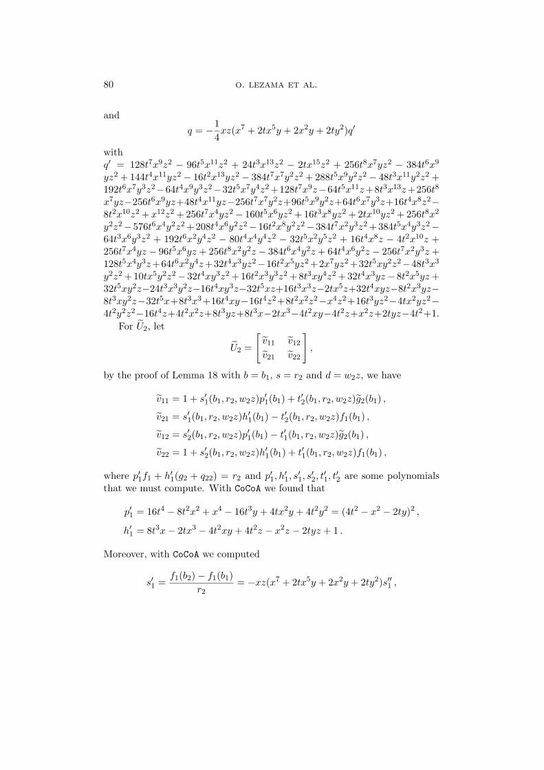
andq = −1
4xz(x7 + 2tx5y + 2x2y + 2ty2)q′
withq′ = 128t7x9z2 − 96t5x11z2 + 24t3x13z2 − 2tx15z2 + 256t8x7yz2 − 384t6x9
yz2 + 144t4x11yz2 − 16t2x13yz2 − 384t7x7y2z2 + 288t5x9y2z2 − 48t3x11y2z2 +192t6x7y3z2−64t4x9y3z2−32t5x7y4z2 +128t7x9z−64t5x11z+8t3x13z+256t8
x7yz−256t6x9yz+48t4x11yz−256t7x7y2z+96t5x9y2z+64t6x7y3z+16t4x8z2−8t2x10z2 + x12z2 + 256t7x4yz2− 160t5x6yz2 + 16t3x8yz2 + 2tx10yz2 + 256t8x2
y2z2−576t6x4y2z2 +208t4x6y2z2−16t2x8y2z2−384t7x2y3z2 +384t5x4y3z2−64t3x6y3z2 + 192t6x2y4z2 − 80t4x4y4z2 − 32t5x2y5z2 + 16t4x8z − 4t2x10z +256t7x4yz − 96t5x6yz + 256t8x2y2z − 384t6x4y2z + 64t4x6y2z − 256t7x2y3z +128t5x4y3z+64t6x2y4z+32t4x3yz2−16t2x5yz2 +2x7yz2 +32t5xy2z2−48t3x3
y2z2 +10tx5y2z2− 32t4xy3z2 +16t2x3y3z2 +8t3xy4z2 +32t4x3yz− 8t2x5yz +32t5xy2z−24t3x3y2z−16t4xy3z−32t5xz+16t3x3z−2tx5z+32t4xyz−8t2x3yz−8t3xy2z−32t5x+8t3x3+16t4xy−16t4z2+8t2x2z2−x4z2+16t3yz2−4tx2yz2−4t2y2z2−16t4z+4t2x2z+8t3yz+8t3x−2tx3−4t2xy−4t2z+x2z+2tyz−4t2+1.
For U2, let
U2 =
[v11 v12
v21 v22
],
by the proof of Lemma 18 with b = b1, s = r2 and d = w2z, we have
v11 = 1 + s′1(b1, r2, w2z)p′1(b1) + t′2(b1, r2, w2z)g2(b1) ,
v21 = s′1(b1, r2, w2z)h′1(b1)− t′2(b1, r2, w2z)f1(b1) ,
v12 = s′2(b1, r2, w2z)p′1(b1)− t′1(b1, r2, w2z)g2(b1) ,
v22 = 1 + s′2(b1, r2, w2z)h′1(b1) + t′1(b1, r2, w2z)f1(b1) ,
where p′1f1 + h′1(g2 + q22) = r2 and p′1, h′1, s
′1, s
′2, t
′1, t
′2 are some polynomials
that we must compute. With CoCoA we found that
p′1 = 16t4 − 8t2x2 + x4 − 16t3y + 4tx2y + 4t2y2 = (4t2 − x2 − 2ty)2 ,
h′1 = 8t3x− 2tx3 − 4t2xy + 4t2z − x2z − 2tyz + 1 .
Moreover, with CoCoA we computed
s′1 =f1(b2)− f1(b1)
r2= −xz(x7 + 2tx5y + 2x2y + 2ty2)s′′1 ,
quillen-suslin rings 81
where
s′′1 := 8t3x9z − 2tx11z + 16t4x7yz − 8t2x9yz − 8t3x7y2z + x8z
+ 16t3x4yz − 2tx6yz + 16t4x2y2z − 12t2x4y2z
− 8t3x2y3z + 2x3yz + 2txy2z − 2tx− 2z .
In a similar way we get that
s′2 =g2(b2)− g2(b1)
r2= −xz(x7 + 2tx5y + 2x2y + 2ty2)(4t2 − x2 − 2ty) ,
t′1 =p′1(b2)− p′1(b1)
r2= 0 ,
t′2 =h′1(b2)− h′1(b1)
r2= xz(x7 + 2tx5y + 2x2y + 2ty2)(4t2 − x2 − 2ty) .
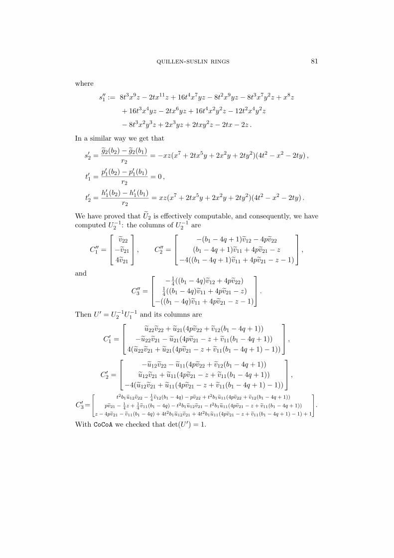
We have proved that U2 is effectively computable, and consequently, we havecomputed U−1
2 : the columns of U−12 are
C ′′1 =
v22
−v21
4v21
, C ′′
2 =
−(b1 − 4q + 1)v12 − 4pv22
(b1 − 4q + 1)v11 + 4pv21 − z
−4((b1 − 4q + 1)v11 + 4pv21 − z − 1)
,
and
C ′′3 =
−14((b1 − 4q)v12 + 4pv22)
14((b1 − 4q)v11 + 4pv21 − z)
−((b1 − 4q)v11 + 4pv21 − z − 1)
.
Then U ′ = U−12 U−1
1 and its columns are
C ′1 =
u22v22 + u21(4pv22 + v12(b1 − 4q + 1))−u22v21 − u21(4pv21 − z + v11(b1 − 4q + 1))
4(u22v21 + u21(4pv21 − z + v11(b1 − 4q + 1)− 1))
,
C ′2 =
−u12v22 − u11(4pv22 + v12(b1 − 4q + 1))u12v21 + u11(4pv21 − z + v11(b1 − 4q + 1))
−4(u12v21 + u11(4pv21 − z + v11(b1 − 4q + 1)− 1))
,
C ′3 =
t2b1u12v22 − 14v12(b1 − 4q)− pv22 + t2b1u11(4pv22 + v12(b1 − 4q + 1))
pv21 − 14z + 1
4v11(b1 − 4q)− t2b1u12v21 − t2b1u11(4pv21 − z + v11(b1 − 4q + 1))
z − 4pv21 − v11(b1 − 4q) + 4t2b1u12v21 + 4t2b1u11(4pv21 − z + v11(b1 − 4q + 1)− 1) + 1
.
With CoCoA we checked that det(U ′) = 1.
82 o. lezama et al.
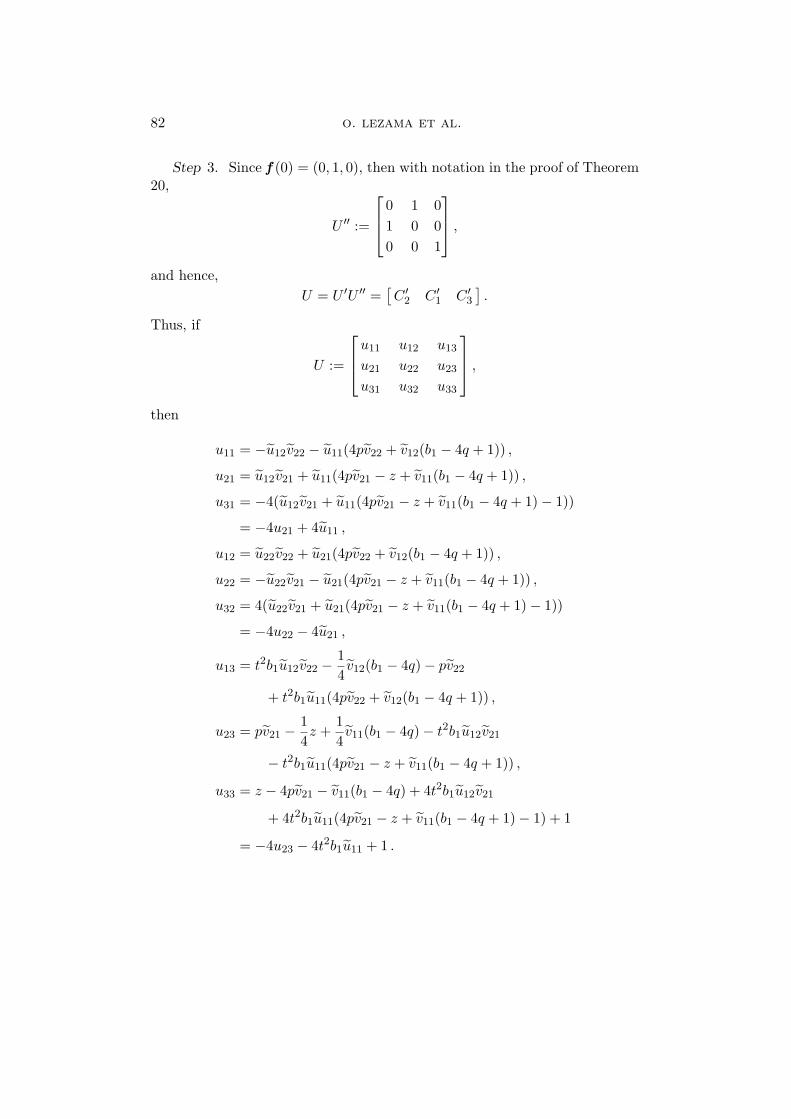
Step 3. Since f (0) = (0, 1, 0), then with notation in the proof of Theorem20,
U ′′ :=
0 1 01 0 00 0 1
,
and hence,U = U ′U ′′ =
[C ′
2 C ′1 C ′
3
].
Thus, if
U :=
u11 u12 u13
u21 u22 u23
u31 u32 u33
,
then
u11 = −u12v22 − u11(4pv22 + v12(b1 − 4q + 1)) ,
u21 = u12v21 + u11(4pv21 − z + v11(b1 − 4q + 1)) ,
u31 = −4(u12v21 + u11(4pv21 − z + v11(b1 − 4q + 1)− 1))
= −4u21 + 4u11 ,
u12 = u22v22 + u21(4pv22 + v12(b1 − 4q + 1)) ,
u22 = −u22v21 − u21(4pv21 − z + v11(b1 − 4q + 1)) ,
u32 = 4(u22v21 + u21(4pv21 − z + v11(b1 − 4q + 1)− 1))
= −4u22 − 4u21 ,
u13 = t2b1u12v22 − 14v12(b1 − 4q)− pv22
+ t2b1u11(4pv22 + v12(b1 − 4q + 1)) ,
u23 = pv21 − 14z +
14v11(b1 − 4q)− t2b1u12v21
− t2b1u11(4pv21 − z + v11(b1 − 4q + 1)) ,
u33 = z − 4pv21 − v11(b1 − 4q) + 4t2b1u12v21
+ 4t2b1u11(4pv21 − z + v11(b1 − 4q + 1)− 1) + 1
= −4u23 − 4t2b1u11 + 1 .
quillen-suslin rings 83
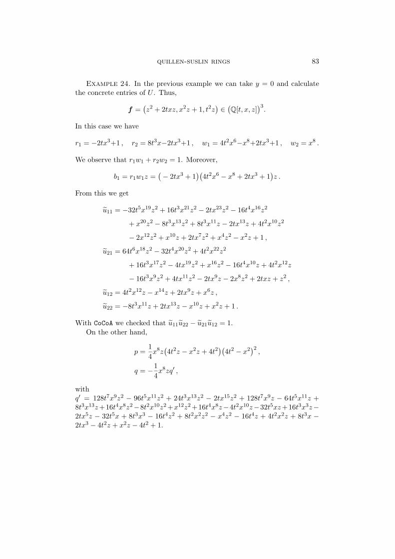
Example 24. In the previous example we can take y = 0 and calculatethe concrete entries of U . Thus,
f =(z2 + 2txz, x2z + 1, t2z
) ∈ (Q[t, x, z]
)3.
In this case we have
r1 = −2tx3+1 , r2 = 8t3x−2tx3+1 , w1 = 4t2x6−x8+2tx3+1 , w2 = x8 .
We observe that r1w1 + r2w2 = 1. Moreover,
b1 = r1w1z =(− 2tx3 + 1
)(4t2x6 − x8 + 2tx3 + 1
)z .
From this we get
u11 = −32t5x19z2 + 16t3x21z2 − 2tx23z2 − 16t4x16z2
+ x20z2 − 8t3x13z2 + 8t3x11z − 2tx13z + 4t2x10z2
− 2x12z2 + x10z + 2tx7z2 + x4z2 − x2z + 1 ,
u21 = 64t6x18z2 − 32t4x20z2 + 4t2x22z2
+ 16t3x17z2 − 4tx19z2 + x16z2 − 16t4x10z + 4t2x12z
− 16t3x9z2 + 4tx11z2 − 2tx9z − 2x8z2 + 2txz + z2 ,
u12 = 4t2x12z − x14z + 2tx9z + x6z ,
u22 = −8t3x11z + 2tx13z − x10z + x2z + 1 .
With CoCoA we checked that u11u22 − u21u12 = 1.On the other hand,
p =14x8z
(4t2z − x2z + 4t2
)(4t2 − x2
)2,
q = −14x8zq′ ,
withq′ = 128t7x9z2 − 96t5x11z2 + 24t3x13z2 − 2tx15z2 + 128t7x9z − 64t5x11z +8t3x13z+16t4x8z2−8t2x10z2 +x12z2 +16t4x8z−4t2x10z−32t5xz+16t3x3z−2tx5z − 32t5x + 8t3x3 − 16t4z2 + 8t2x2z2 − x4z2 − 16t4z + 4t2x2z + 8t3x −2tx3 − 4t2z + x2z − 4t2 + 1.
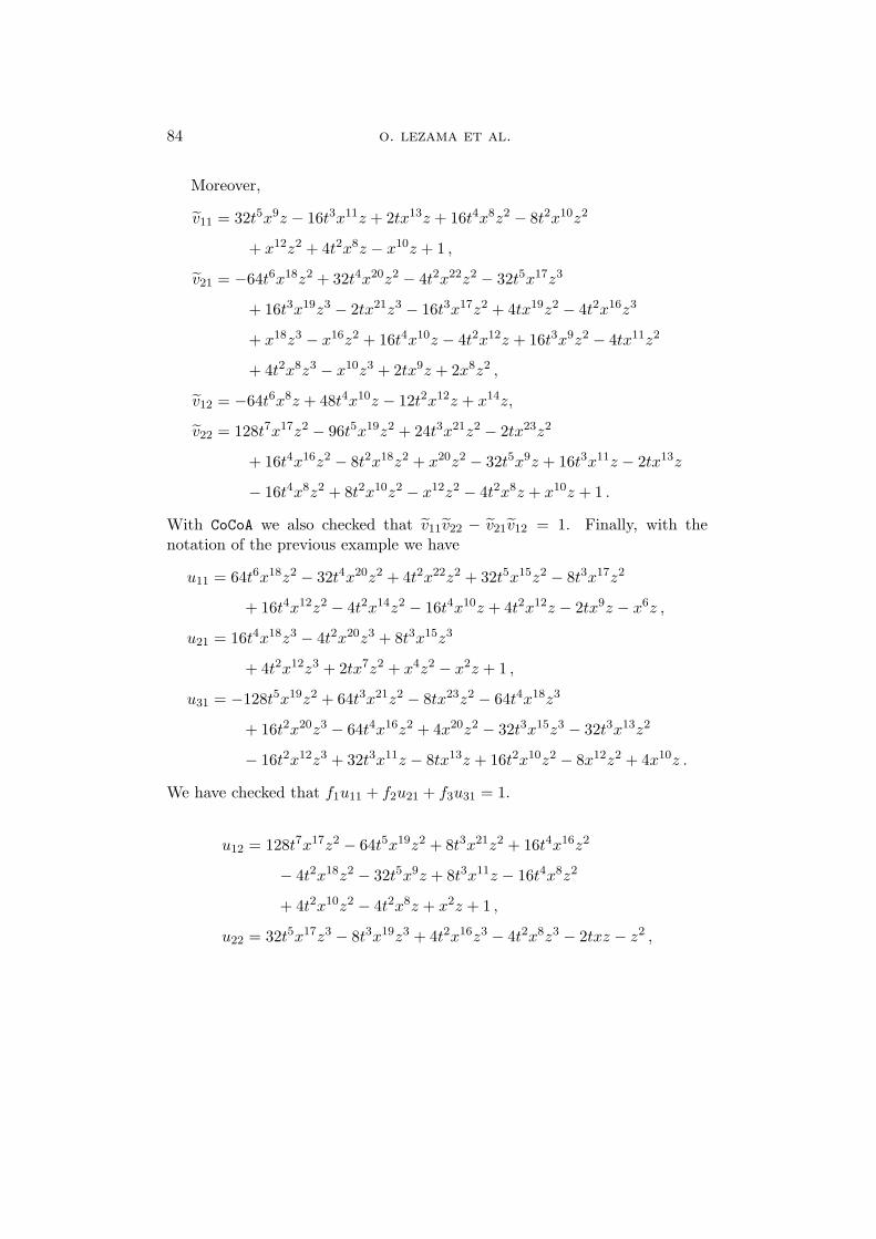
84 o. lezama et al.
Moreover,
v11 = 32t5x9z − 16t3x11z + 2tx13z + 16t4x8z2 − 8t2x10z2
+ x12z2 + 4t2x8z − x10z + 1 ,
v21 = −64t6x18z2 + 32t4x20z2 − 4t2x22z2 − 32t5x17z3
+ 16t3x19z3 − 2tx21z3 − 16t3x17z2 + 4tx19z2 − 4t2x16z3
+ x18z3 − x16z2 + 16t4x10z − 4t2x12z + 16t3x9z2 − 4tx11z2
+ 4t2x8z3 − x10z3 + 2tx9z + 2x8z2 ,
v12 = −64t6x8z + 48t4x10z − 12t2x12z + x14z,
v22 = 128t7x17z2 − 96t5x19z2 + 24t3x21z2 − 2tx23z2
+ 16t4x16z2 − 8t2x18z2 + x20z2 − 32t5x9z + 16t3x11z − 2tx13z
− 16t4x8z2 + 8t2x10z2 − x12z2 − 4t2x8z + x10z + 1 .
With CoCoA we also checked that v11v22 − v21v12 = 1. Finally, with thenotation of the previous example we have
u11 = 64t6x18z2 − 32t4x20z2 + 4t2x22z2 + 32t5x15z2 − 8t3x17z2
+ 16t4x12z2 − 4t2x14z2 − 16t4x10z + 4t2x12z − 2tx9z − x6z ,
u21 = 16t4x18z3 − 4t2x20z3 + 8t3x15z3
+ 4t2x12z3 + 2tx7z2 + x4z2 − x2z + 1 ,
u31 = −128t5x19z2 + 64t3x21z2 − 8tx23z2 − 64t4x18z3
+ 16t2x20z3 − 64t4x16z2 + 4x20z2 − 32t3x15z3 − 32t3x13z2
− 16t2x12z3 + 32t3x11z − 8tx13z + 16t2x10z2 − 8x12z2 + 4x10z .
We have checked that f1u11 + f2u21 + f3u31 = 1.
u12 = 128t7x17z2 − 64t5x19z2 + 8t3x21z2 + 16t4x16z2
− 4t2x18z2 − 32t5x9z + 8t3x11z − 16t4x8z2
+ 4t2x10z2 − 4t2x8z + x2z + 1 ,
u22 = 32t5x17z3 − 8t3x19z3 + 4t2x16z3 − 4t2x8z3 − 2txz − z2 ,
quillen-suslin rings 85
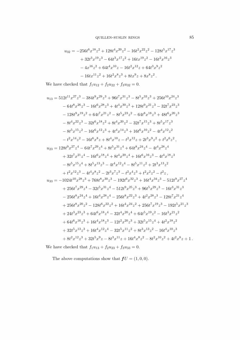
u32 = −256t6x18z2 + 128t4x20z2 − 16t2x22z2 − 128t5x17z3
+ 32t3x19z3 − 64t3x17z2 + 16tx19z2 − 16t2x16z3
− 4x16z2 + 64t4x10z − 16t2x12z + 64t3x9z2
− 16tx11z2 + 16t2x8z3 + 8tx9z + 8x8z2 .
We have checked that f1u12 + f2u22 + f3u32 = 0.
u13 = 512t11x27z3 − 384t9x29z3 + 96t7x31z3 − 8t5x33z3 + 256t10x24z3
− 64t8x26z3 − 16t6x28z3 + 4t4x30z3 + 128t9x21z3 − 32t7x23z3
− 128t9x19z2 + 64t7x21z2 − 8t5x23z2 − 64t8x18z3 + 48t6x20z3
− 8t4x22z3 − 32t6x18z2 + 8t4x20z2 − 32t7x15z3 + 8t5x17z3
− 8t5x15z2 − 16t6x12z3 + 4t4x14z3 + 16t6x10z2 − 4t4x12z2
− t2x14z2 − 16t6x8z + 8t4x10z − t2x12z + 2t3x9z2 + t2x6z2 ,
u23 = 128t9x27z4 − 64t7x29z4 + 8t5x31z4 + 64t8x24z4 − 4t4x28z4
+ 32t7x21z4 − 16t6x18z4 + 8t4x20z4 + 16t6x16z3 − 4t4x18z3
− 8t5x15z4 + 8t5x13z3 − 4t4x12z4 − 8t5x11z2 + 2t3x13z2
+ t2x12z3 − 4t4x8z2 − 2t3x7z3 − t2x4z3 + t2x2z2 − t2z ,
u33 = −1024t10x28z3 + 768t8x30z3 − 192t6x32z3 + 16t4x34z3 − 512t9x27z4
+ 256t7x29z4 − 32t5x31z4 − 512t9x25z3 + 96t5x29z3 − 16t3x31z3
− 256t8x24z4 + 16t4x28z4 − 256t8x22z3 + 4t2x28z3 − 128t7x21z4
+ 256t8x20z2 − 128t6x22z2 + 16t4x24z2 + 256t7x19z3 − 192t5x21z3
+ 24t3x23z3 + 64t6x18z4 − 32t4x20z4 + 64t5x19z2 − 16t3x21z2
+ 64t6x16z3 + 16t4x18z3 − 12t2x20z3 + 32t5x15z4 + 4t2x18z2
+ 32t5x13z3 + 16t4x12z4 − 32t5x11z2 + 8t3x13z2 − 16t4x10z3
+ 8t2x12z3 + 32t5x9z − 8t3x11z + 16t4x8z2 − 8t2x10z2 + 4t2x8z + 1 .
We have checked that f1u13 + f2u23 + f3u33 = 0.
The above computations show that f U = (1, 0, 0).
86 o. lezama et al.
Remark 25. In [7] has been recently implemented the packageQUILLENSUSLIN developed in the computer algebra system MAPLE, that willappear soon. The main functions of the package QUILLENSUSLIN are: computea unimodular matrix U which transforms a row vector admitting a right-inverse into a matrix of the form [ I 0 ]; complete a matrix admitting a right-inverse to a unimodular matrix; compute a basis of a free module finitelypresented by a given matrix.
We conclude this section commenting some recent generalizations of theQuillen-Suslin theorem: Gago-Vargas in [11] extended the algorithmic proofsof the Quillen-Suslin theorem to coefficients in a PID with some additionalcomputational conditions. In [14] Gubeladze presented a non algorithmicproof that the monoid ring D[M ] is PF, where D is a PID and M is a certaintype of commutative monoid; in [22] is presented an algorithmic proof of theGubeladze’s generalization for fields. In [20] is presented an algorithmic prooffor quotients rings of K[x1, . . . , xn] by monomials ideals. When D is a PID,quotients rings of D[M ] by monomials ideals are also PF. A non algorithmicproof of this fact is given in [32]. According to these results arise the followingproblem-conjecture.
Conjecture 26. The constructive proofs in [11] and [20] can be extendedto D[M ]/I, where D is a PID and M is a commutative, seminormal, finitelygenerated monoid, which is torsion free, cancellative, and has no nontrivialunits.
4. Extended rings and the Bass-Quillen conjecture
If we consider finitely generated projective modules over arbitrary com-mutative polynomial rings, is natural to ask if the Quillen-Suslin theorem alsoholds, i.e., if S is an arbitrary commutative ring, we ask if S is a QS ring.Related with this question are defined the extended modules and the corre-spondent extended rings (see [18]). In this section we will study these topicsand some related conjectures.
Definition 27. Let S be a commutative ring and B a S-algebra. Let Mbe a B-module, M es extended from S if there exists a S-module M0 suchthat M ∼= M0 ⊗S B.
With the notation of the previous definition and setting
S[X] := S[x1, . . . , xn] and 〈X〉 := 〈x1, . . . , xn〉 ,
quillen-suslin rings 87
we have the following properties.
Proposition 28. (i) If M is free over B, then M is extended from S.
(ii) If B = S[X] and M is extended from S, then
M0∼= M/〈X〉M .
Moreover, if M is finitely generated (projective) as B-module, then M0
is finitely generated (projective) as S-module.
Proof. (i) If M ∼= B(Y ), then M ∼= S(Y ) ⊗S B.(ii) If M ∼= M0 ⊗S S[X] then
M ⊗S[X] S[X]/〈X〉 ∼= M0 ⊗S S[X]⊗S[X] S[X]/〈X〉 ,M/〈X〉M ∼= M0 ⊗S S[X]/〈X〉 ,M/〈X〉M ∼= M0 ⊗S S ,
M/〈X〉M ∼= M0 .
Let M = 〈z1, . . . , zt〉 and w ∈ M0, then w = z with z ∈ M ; there exist poly-nomials p1(X), . . . , pt(X) ∈ S[X] such that w = z = z1p1(X) + · · ·+ ztpt(X)= z1p01 + · · · + ztp0t, where p0i is the independent term of pi(X), 1 ≤ i ≤ t.Hence, M0 = 〈z1, . . . , zt〉.
Finally, let M ⊕M ′ = (S[X])(Y ), then
(M ⊕M ′)⊗S[X] S[X]/〈X〉 ∼= (S[X])(Y ) ⊗S[X] S[X]/〈X〉 ,
M0 ⊕M ′/〈X〉M ′ ∼= S(Y ) .
Extended modules are close related with QS rings as is showed in thefollowing results (see [18]).
Definition 29. Let S be a commutative ring.
(i) Let n ≥ 1, S is a En ring if every f.g. projective S[x1, . . . , xn]-module isextended from S.
(ii) S is an extended ring E, if S is En for each n ≥ 1.
88 o. lezama et al.
From Proposition 28 we get the following consequences:
E =⋂
n≥1
En , (4.1)
QSn ⊆ En for each n ≥ 1 , (4.2)
QS ⊆ E . (4.3)
The following results are announced without proof in [18, p. 166].
Theorem 30. (i) QS = PF ∩ E = PSF ∩H ∩ E.
(ii) Let S a PF ring. Then, for each n ≥ 1, S is En if and only if S[x1, . . . , xn]is PF. In other words, for PF rings En = QSn for each n ≥ 1, andconsequently, E = QS.
(iii) For each n ≥ 1, if S is En+1, then S and S[x] are En.
(iv) E ⊆ · · · ⊆ En+1 ⊆ En ⊆ · · · ⊆ E1.
Proof. (i) First we will prove that QS ⊆ PF ∩ E. By (4.3), QS ⊆ E; letM be a S-f.g. projective module, then M ⊕M ′ ∼= Sm and hence
(M ⊕M ′)⊗S S[X] ∼= Sm ⊗S S[X] ,
(M ⊗S S[X]⊕M ′ ⊗S S[X]) ∼= (S ⊗S S[X])m ∼= S[X]m ;
this means that M ⊗S S[X] is a S[X]-f.g. projective module, so by the hy-pothesis M ⊗S S[X] is a S[X]-free module, i.e., M ⊗S S[X] ∼= S[X]k, for somek ≥ 0. From this we get
M ⊗S S[X]⊗S[X] S[X]/〈X〉 ∼= S[X]k ⊗S[X] S[X]/〈X〉 ,
M ⊗S (S[X]⊗S[X] S[X]/〈X〉) ∼= (S[X]⊗S[X] S[X]/〈X〉)k ,
M ⊗S S[X]/〈X〉 ∼= (S[X]/〈X〉)k ,
M ⊗S S ∼= M ∼= Sk .
This means that S is PF. Thus, QS ⊆ PF, and hence, QS ⊆ PF ∩ E.Now we will prove that PF ∩ E ⊆ QS: let M be a S[X]-f.g. projective
module, then M is extended from S and there exists a S-f.g. projective moduleM0 such that M ∼= M0⊗SS[X]. By the hypothesis, M is S-free, i.e., M0
∼= Sm,
quillen-suslin rings 89
for some m ≥ 0. Hence, M ∼= Sm ⊗S S[X] ∼= S[X]m, i.e., M is S[X]-free.This prove that S is QS.
The second equality follows from (2.1).(ii) “⇒” Let M be a f.g. projective S[X]-module, then M is extended from
S and theres exists a f.g. projective S-module M0 such that M ∼= M0⊗S S[X].We are assuimng that S is PF, then M0 is S-free, and hence, M is S[X]-free.This proves that En ⊆ QSn for each n ≥ 1. The converse is thrue becauseof (4.2).
(iii) Let M be a f.g. projective S[X]-module, the there exists a S[X]-module M ′ such that M ⊕ M ′ ∼= (S[X])m for some m ≥ 1. From this weget
(M ⊕M ′)⊗S[X] S[X, xn+1] ∼= S[X]m ⊗S[X] S[X,xn+1] ,
M ⊗S[X] S[X, xn+1]⊕M ′ ⊗S[X] S[X, xn+1] ∼= S[X, xn+1]m .
This means that M⊗S[X]S[X, xn+1] is a f.g. projective S[X, xn+1]-module;since S is En+1, there exists a S-module M0 such that
M ⊗S[X] S[X,xn+1] ∼= M0 ⊗S S[X, xn+1] ,
and from this we get
M ⊗S[X] S[X, xn+1]⊗S[X,xn+1] S[X, xn+1]/〈xn+1〉∼= M0 ⊗S S[X, xn+1]⊗S[X,xn+1] S[X, xn+1]/〈xn+1〉 ,
M ⊗S[X]
(S[X, xn+1]⊗S[X,xn+1] S[X, xn+1]/〈xn+1〉
)
∼= M0 ⊗S
(S[X,xn+1]⊗S[X,xn+1] S[X,xn+1]/〈xn+1〉
),
i.e.,M ⊗S[X] S[X] ∼= M ∼= M0 ⊗S S[X] .
This means that M is extended from S, and hence, S is En.Now let B := S[x] and M be a f.g. projective B[X]-module, the there
exists a B[X]-module M ′ such that M ⊕ M ′ ∼= (B[X])m for some m ≥ 1.From this we get
(M ⊕M ′)⊗B[X] S[X, x] ∼= B[X]m ⊗B[X] S[X,x] ,
M ⊗B[X] S[X,x]⊕M ′ ⊗B[X] S[X, x] ∼=(B[X]⊗B[X] S[X,x]
)m ∼= S[X, x]m .
90 o. lezama et al.
But B[X] = S[X, x], soM ⊕M ′ ∼= S[X,x]m ,
i.e., M is a f.g. projective S[X, x]-module. This implies that M is extendedfrom S; thus, there exists M0 a f.g. projective S-module such that M ∼=M0 ⊗S S[X, x]. Hence,
M ∼= M0 ⊗S
(S[x]⊗S[x] S[X, x]
),
M ∼=(M0 ⊗S S[x]
)⊗S[x] S[x][X] ,
M ∼= M ′0 ⊗B B[X] ,
with M ′0 := M0 ⊗S S[x] = M0 ⊗S B.
(iv) This is consequence of (iii) and (4.1).
From this theorem arise the following conjectures.
Conjectures 31. (i) For each n ≥ 1, if S is En, then S[x] is En.(ii) If S is E, then S[x] is E.(iii) E1 = E2.(iv) E1 = Em for some m ≥ 2.(v) E1 = E.
Related with these questions are the following properties (see [18]).
Proposition 32. For a fixed integer n ≥ 1, the following four statementsare equivalent:
(i) Any ring satisfying En also satisfies En+1.
(ii) Any ring satisfying En also satisfies En+r for all r ≥ 1.
(iii) If a ring S satisfies En, then so does S[x].
(iv) If a ring S satisfies En, then so does S[x1, . . . , xr] for all r ≥ 1.
Proof. (i) ⇒ (iii) : Let S be an En ring, then S is an En+1 ring. Thus,any f.g. projective S[x][X]-module is extended from S, so S[x] is En.
(iii) ⇒ (i) : Let S be an En ring, and let M be an S[x1, . . . , xn+1]-f.g.proyective module; since S[x1] is En, then M is extended from S[x1], i.e.,
M ∼= M1 ⊗S[x1] S[x1][x2, . . . , xn+1] ,
quillen-suslin rings 91
where M1 is a f.g. projective S[x1]-module. Since S is En, so by Theorem 30(iv), S is E1, hence M1 is extended form S, and consequently, M is extendedfrom S. This means that S is En+1.
(i) ⇒ (ii) : Let S ∈ En, then S ∈ En+1, thus the result is obvious for r = 1.Since S ∈ En+1, by Theorem 30, S[x1] ∈ En and again by (i), S[x1] ∈ En+1.We have proved (iii) for n + 1, but (iii) is equivalent to (i) for a fixed integer,in this case for the integer n + 1, then by (i) S ∈ En+2. Thus, we have provedthat En+1 = En+2. Since S ∈ En+2, then by Theorem 30, S[x] ∈ En+1, soS[x] ∈ En+2. We have proved (iii) for n + 2, but (iii) is equivalent to (i) for afixed integer, in this case for the integer n + 2, then by (i) S ∈ En+3. We canrepeat this reasoning and we get that S ∈ En+r, for each r ≥ 1.
(ii) ⇒ (i) : Obvious.(iii) ⇒ (iv) : If S ∈ En then by (iii) S[x1] ∈ En, and again by (iii)
S[x1, x2] ∈ En. By induction on r we complete the proof of this part.(iv) ⇒ (iii) : Obvious.
Corollary 33. With the notation of Conjectures 31, it holds:
(a) (iii) ⇔ (iv) ⇔ (v).(b) (v) ⇒ (i) ⇒ (ii).
Proof. (a) (iii) ⇒ (iv) : It is clear that Em ⊆ E1; let S ∈ E1, then by(iii), S ∈ E2. Using Proposition 32 with n = 1, we get that S ∈ Er for r ≥ 1,i.e., S ∈ Em.
(iv) ⇒ (iii) : It is clear that E2 ⊆ E1; let S ∈ E1, then by (iv), S ∈ Em
⊆ E2.(iii) ⇒ (v) : This proof is similar to previous proof.(b) (v) ⇒ (i) : Let S ∈ En, then S ∈ E1 = E, so S ∈ En+1; by Proposition
32, S[x] ∈ En.(i) ⇒ (ii) : Obvious.
Some non trivial examples of E rings are the followings.
Examples 34. (i) Any Prufer domain (every f.g. ideal is projective) isa E ring (see [23] and [8]). We observe that the Quillen-Suslin theorem is aconsequence of this result: in fact, if D is a PID, then D is a Prufer domain;let M be a f.g. projective D[X]-module, by the result M is extended from D,i.e., M ∼= M0 ⊗D D[X], where M0 is a f.g. projective D-module. But since Dis a PID, M0 is D-free, and consequently, M is D[X]-free.
92 o. lezama et al.
(ii) Bezout domains are Prufer domains. Thus, Bezout domains are E;however, if D is a Bezout domain, any f.g. projective D[X]-module is free,i.e., the Bezout domains are QS (see [26]).
(iii) Let S be a commutative ring of Krull dimension 0. Then, S is E(see [18])
(iv) A Noetherian generalization of the Quillen-Suslin theorem has beengiven also by Quillen and Suslin (see [18]). Let S be a commutative regularring of Krull dimension ≤ 2. Then, S is E. We note that the Quillen-Suslintheorem is a consequence of this result. In fact, any PID satisfies the con-ditions of the result: we recall that a commutative ring S is regular if S isNoetherian and the global dimension of S is finite (see [18] and [29]). But anyPID is Noetherian and any PID has global dimension ≤ 1. Thus, any PIDis regular; moreover, the Krull dimension of any PID is ≤ 1. Thus, if D isa PID, then every finitely generated projective D[X]-module M is extendedfrom D, and as we saw above, this implies that M is D[X]-free.
Related with the results of previous example, Bass ([2]) and Quillen ([28])formulated the following conjecture.
Conjecture 35. (BQd: The Bass-Quillen conjecture) Let S be acommutative regular ring of Krull dimension ≤ d. Then, every finitely gener-ated projective S[X]-module is extended from S, i.e., S is E.
The H property and the BQd conjecture are related in the following way.
Theorem 36. The following conjectures are equivalent:
(C1) If S is H then S[x] is H.
(C2) If S is local, then S[x] is H.
(C3) If S is a commutative ring and M is a stably free S[x]-module, then Mis extended from S.
(C4) If S is local and M is a stably free S[x]-module, then M is extendedfrom S.
(C5) If S is a commutative ring and f = (f1(x), . . . , fn(x))T is an unimodularcolumn matrix over S[x] such that f(0) can be completed to a matrix ofGLn(S), then f can be completed to a matrix of GLn(S[x]).
(C6) If S is local and f = (f1(x), . . . , fn(x))T is an unimodular column matrixover S[x] such that f(0) can be completed to a matrix of GLn(S), thenf can be completed to a matrix of GLn(S[x]).
quillen-suslin rings 93
Morever, the truth of any of these conjectures will imply the truth of BQd
for all d.
Proof. (C1) ⇒ (C2) : Let M be a stably free S-module, then M is a f.g.projective S-module, but since S is local then M is S-free. Thus, S has theH property. By (C1), S[x] is H.
(C2) ⇒ (C4) : Let M be a stably free S[x]-module, with S local; by(C2), S[x] is H, then M is S[x]-free, and hence, M is extended from S (seeProposition 28).
(C4) ⇒ (C2) : Let M be a stably free S[x]-module, then M is a f.g.projective S[x]-module; by (C4), M is extended from S, M ∼= M0 ⊗S S[x],where M0 is a f.g. projective S-module. But since S is local, then M0 is S-free,so M is S[x]-free.
(C4) ⇒ (C3) : This is a consequence of the Quillen Patching theorem: LetS be a commutative ring. Let M be a finitely presented S[X]-module. Then,M is extended from S if and only if for every maximal ideal P ∈ Max(S), MP
is extended from SP (see [18]). In fact, let M be a stably free S[x]-module,then M is a finitely presented module; moreover, MP is a stably free SP [x]-module for each maximal ideal P of S: S[x]m ∼= M ⊕S[x]n for some m,n ≥ 0,then Sp[x]m ∼= Mp ⊕ Sp[x]n. By (C4), MP is extended from SP , and by theQuillen Patching theorem, M is extended from S.
(C3) ⇒ (C1) : Let S be a H ring; let M be a stably free S[x]-module; by(C3), M is extended from S, M ∼= M0 ⊗S S[x], where M0 is a f.g. projectiveS-module. We need to prove that M is S[x]-free. We have S[x]p ∼= M ⊕S[x]q
for some p, q ≥ 0; then
S[x]p ∼= (M0 ⊗S S[x])⊕ S[x]q ,
and hence
S[x]p ⊗S[x] S[x]/〈x〉 ∼= (M0 ⊗S S[x])⊗S[x] S[x]/〈x〉 ⊕ S[x]q ⊗S[x] S[x]/〈x〉 ,i.e.,
Sp ∼= M0 ⊕ Sq ,
This means that M0 is a stably free S-module, but since S is H, then M0 isS-free, and hence, M is S[x]-free.
(C3) ⇒ (C5) : There exists g = (g1(x), . . . , gn(x)) such that g1(x)f1(x) +· · ·+ gn(x)fn(x) = 1, we define
S[x]n α−−→ S[x]e i 7−→ gi(x)

94 o. lezama et al.
where {e1, . . . , en} is the canonical basis of S[x]n. We observe that α in asurjective homomorphism since α(f ) = 1. There exists β : S[x] → S[x]n
such that αβ = iS[x] and S[x]n = Im(β) ⊕ ker(α). In fact, β is defined byβ(1) := f and β is injective, hence, Im(β) ∼= S[x] is free with basis {f }.This implies that ker(α) is stably free, and by hypothesis, ker(α) is extendedfrom S. So, there exists a S-module K0 such that ker(α) ∼= K0 ⊗S S[x],moreover K0
∼= ker(α)/〈x〉 ker(α). If we prove that ker(α)/〈x〉 ker(α) is S-free, then ker(α) is S[x]-free, and consequently, {f ,h1, . . . ,hn−1} is a basisif S[x]n, where {h1, . . . ,hn−1} is a basis of ker(α). This means that B :=[f h1 · · ·hn−1] ∈ GLn(S[x]) and (C5) holds.
Thus, we must prove that ker(α)/〈x〉 ker(α) is S-free. We define
Sn α0−−→ S
e i 7−→ gi(0)
where {e1, . . . , en} is the canonical basis of Sn. There exists β0 : S → Sn
such that α0β0 = iS and Sn = Im(β0) ⊕ ker(α0). In fact, β0 is defined byβ0(1) := f (0) and β0 is injective, hence, Im(β0) ∼= S is free with basis {f (0)}.Thus,
Sn = ker(α0)⊕ 〈f (0)〉 ;but by hypothesis f (0) is completable to a square matrix of GLn(S), then aswe saw in the proof of Theorem 11, ker(α0) ∼= Sn−1. The idea is to prove thatker(α)/〈x〉 ker(α) ∼= ker(α0). We have the following commutative diagram:
S[x]n ⊗ (S[x]/〈x〉) α⊗i−−−−→ S[x]⊗ (
S[x]/〈x〉)
φ
yyϕ
Sn α0−−−−→ S
where i is the identical map of S[x]/〈x〉 and the vertical arrows φ and ϕ arethe natural isomorphisms defined by
φ((h1(x), . . . , hn(x))⊗ 1
)= (h1(0), . . . , hn(0)) ,
ϕ(h(x)⊗ 1
)= h(0) .
Then we have
ker(α0) ∼= ker(α⊗ i) = ker(α)⊗ (S[x]/〈x〉) = ker(α)/〈x〉 ker(α) .
(C5) ⇒ (C6) : Obvious.
quillen-suslin rings 95
(C6) ⇒ (C2) : We will apply again Theorem 11. If f = (f1(x), . . . , fn(x))T
is an unimodular column matrix over R[x], then there exists gi(x) ∈ S[x],1 ≤ i ≤ n, such that g1(x)f1(x) + · · ·+ gn(x)fn(x) = 1, so g1(0)f1(0) + · · ·+gn(0)fn(0) = 1. Since S is local there exists i such that fi(0) ∈ S∗, andhence, by elementary operations on the rows of f (0) we find an invertiblematrix B ∈ GLn(S) such that Bf(0) = e1, i.e., f (0) can be completed to aninvertible matrix of GLn(S). By (C6), f can be completed to an invertiblematrix of GLn(S[x]).
The proof of the second part of theorem is very extensive and need manypreliminaries; this proof can be read in [18].
According to previous theorem, if the conjecture (C6) is true then theBass-Quillen conjecture is true, and also, the Conjecture 16. The conjec-ture (C6) can be formulated in the following way: in a local ring S if f =(f1(x), . . . , fn(x))T is an unimodular column matrix over R[x], then
f1(0)...
fn(0)
= Be1 ⇒
f1(x)...
fn(x)
= Be1 ,
where B ∈ GLn(S) and B ∈ GLn(S[x]).
References
[1] W.W. Adams, P. Loustaunau, “An Introduction to Grobner Bases ”,Graduate Studies in Mathematics, No. 3, AMS, Providence, RI, 1994.
[2] H. Bass, Some Problems in “classical” algebraic K-theory, in “ AlgebraicK-Theory, II ”, Lecture Notes in Math., Vol. 342, Springer, Berlin, 1973,3 – 73.
[3] S. Bhatwadekar, R. Rao, On a question of Quillen, Trans. Amer. Math.Soc. 279 (1983), 801 – 810.
[4] J. Brewer, J. Bunce, F. Van Vleck, “Linear Systems over Commu-tative Rings ”, Lecture Notes in Pure and Applied Mathematics, No. 104.Marcel Dekker, Inc., New York, 1986.
[5] W. Brown, “Matrices over Commutative Rings ”, Marcel Dekker, Inc., NewYork, 1993.
[6] A. Fabianska, A. Quadrat, Applications of the Quillen-Suslin theoremto multidimensional systems theory, in “Grobner Bases in Control Theoryand Signal Processing ”, Radon Ser. Comput. Appl. Math., 3, Walter deGruyter, Berlin, 2007, 23 – 106.
[7] A. Fabianska, QuillenSuslin project: A package for computing bases offree modules over commutative polynomial rings :http://wwwb.math.rwth-aachen.de/QuillenSuslin
96 o. lezama et al.
[8] M. Fontana, J.A. Huckaba, I.J. Papick, “ Prufer Domains ”, Monogr.Textbooks Pure Appl. Math., No. 203, Marcel Dekker, Inc., New York,1997.
[9] W. Fulton, “Algebraic Curves. An Introduction to Algebraic Geometry ”,W.A. Benjamin, Inc., New York-Amsterdam, 1969.
[10] J. Gago-Vargas, Bases for projective modules in An(k), J. Symbolic Com-put. 36 (2003), 845 – 853.
[11] J. Gago-Vargas, Constructions in R[x1, . . . , xn]: applications to K-theory,J. Pure Appl. Algebra 171 (2002), 185 – 196.
[12] J. Gago-Vargas, On Suslin’s stability theorem for R[x1, . . . , xm], in “ RingTheory and Algebraic Geometry (Leon, 1999) ”, Lecture Notes in Pure andApplied Mathematics, No. 221, Dekker, New York, 2001, 203 – 210.
[13] G. Greuel, G. Pfister, “A Singular Introduction to Commutative Alge-bra, 2nd edition ”, Springer, Berlin, 2007.
[14] I. Gubeladze, The Anderson conjecture and a maximal class of monoidsover which projective modules are free, Math. USSR Sb. 63 (1989), 165 –180.
[15] http://CoCoA.dima.unige.it
[16] http://www.singular.uni-kl.de
[17] E. Kunz, “ Introduction to Commutative Algebra and Algebraic Geometry “,Birkhauser Boston, Inc., Boston, MA, 1985.
[18] T.Y. Lam, “ Serre’s Problem on Projective Modules ”, Springer Monogr.Math., Springer-Verlag, Berlin, 2006.
[19] S. Lang, “Algebra ”, Grad. Texts in Math., No. 211, Springer-Verlag, NewYork, 2002.
[20] R.C. Laubenbacher, K. Schlauch, An algorithm for the Quillen-Suslintheorem for quotients of polynomial rings by monomial ideals, J. SymbolicComput. 30 (2000), 555 – 571.
[21] R.C. Laubenbacher, C. Woodburn, A new algorithm for the Quillen-Suslin theorem, Beitrage Algebra Geom. 41 (2000), 23 – 31.
[22] R.C. Laubenbacher, C. Woodburn, An algorithm for the Quillen-Suslin theorem for monoid rings, J. Pure Appl. Algebra 117-118 (1997),395 – 429.
[23] Y. Lequain, A. Simis, Projective modules over R[x1, . . . , xn], R a Pruferdomain, J. Pure Appl. Algebra 18 (1980), 165 – 171.
[24] A. Logar, B. Sturmfels, Algorithms for the Quillen-Suslin theorem, J.Algebra 145 (1) (1992), 231 – 239.
[25] B. McDonald, “Linear Algebra over Commutative Rings ”, Monogr. Text-books Pure Appl. Math., No. 87, Marcel Dekker, 1984.
[26] P. Maroscia, Modules projectifs sur certains anneaux de polynomes, C.R.Acad. Sci. Paris, Ser. A-B 285 (4) (1977), A183 – A185.
[27] H. Park, C. Woodburn, An algorithmic proof of Suslin’s stability theo-rem for polynomial rings, J. Algebra 178 (1995), 277 – 298.
quillen-suslin rings 97
[28] D. Quillen, Proyective modules over polynomial rings, Invent. Math. 36(1976), 167 – 171.
[29] J.J. Rotman, “An Introduction to Homological Algebra ”, Pure Appl.Math., No. 85, Academic Press, Inc., New York-London, 1979.
[30] J.P. Serre, Faisceaux algebriques coherents, Ann. of Math. 61 (1955), 197 –278.
[31] A.A. Suslin, Proyective modules over polynomial rings are free, Soviet Math.Dokl. 17 (1976), 1160 – 1164.
[32] R.G. Swan, Gubeladze’s proof of Anderson’s conjecture, in “ Azumaya Al-gebras, Actions and Modules (D. Haile and J. Osterburg eds.) ”, Contemp.Math., No. 124 , Amer. Math. Soc., Providence, RI, 1992, 215 – 250


![The Quillen-Suslin Theoremdiposit.ub.edu/dspace/bitstream/2445/125803/2/memoria.pdf · proved, just three years later, that projective modules over k[x1,. . ., xn] are stably free](https://img.pdfslide.us/doc/110x75/5f15ae38e9258750663f7d32/the-quillen-suslin-proved-just-three-years-later-that-projective-modules-over.jpg)