GEOMETRIC MECHANICS, DYNAMICS, AND CONTROLOF FISHLIKE SWIMMING IN A PLANAR IDEAL FLUID

SCOTT DAVID KELLY∗, PARTHESH PUJARI† , AND HAILONG XIONG‡

Abstract. We summarize the geometric treatment of locomotion in an ideal fluidin the absence of vorticity and link this work to a planar model incorporating localizedvortex shedding evocative of vortex shedding from the caudal fin of a swimming fish.We present simulations of open-loop and closed-loop navigation and energy-harvestingby a Joukowski foil with variable camber shedding discrete vorticity from its trailing tip.

Key words. Geometric mechanics, vortex dynamics, locomotion.

AMS(MOS) subject classifications. Primary 70H33, 76B47, 93C10

1. Introduction. In this paper, we present an idealized model for pla-nar fishlike swimming and explore the dynamics and control of this model.The model represents the synthesis of two lines of research pertaining toideal hydrodynamics, one addressing the locomotion of free deformablebodies in the absence of vorticity and the other addressing the interactionof free rigid bodies with systems of discrete vorticity. The paper beginswith a survey of concepts arising in this earlier work, focused in particularon the realization of locomotion problems in terms of analytical mechan-ics and nonlinear control systems on differentiable manifolds. The lattersections of the paper focus on the computational study of idealized fishlikeswimming with an eye toward simple feedback control design for navigationand energy harvesting.

2. The Geometric View of Locomotion. A mathematical frame-work for modeling the locomotion of a deformable body can be derived fromthe geometry of the space in which the variables parametrizing the problemreside. Implicit in the following discussion are the smoothness assumptionsneeded to justify our regarding this space and various subspaces thereof asdifferentiable manifolds. The material that follows has been addressed inmathematical detail elsewhere [4]; we endeavor to summarize the essentialconcepts with only as much detail as is needed for practical calculations.

2.1. Configuration Space as a Principal Fiber Bundle. We re-fer to a time-parametrized curve in a manifold as a trajectory and the imageof this curve — in other words, the sequential locus of points it comprises,

∗Department of Mechanical Engineering and Engineering Science, University of NorthCarolina at Charlotte, Charlotte, North Carolina 28205.†Department of Mechanical Engineering and Engineering Science, University of North

Carolina at Charlotte, Charlotte, North Carolina 28205.‡Quantitative Risk Management, Inc., Chicago, Illinois 60602. The work of all three

authors was supported in part by NSF grant CMMI 04-49319.

1

2 SCOTT DAVID KELLY, PARTHESH PUJARI, and HAILONG XIONG

without regard to time parametrization — as a path. We regard the in-stantaneous shape of a deformable body — distinct from its position ororientation relative to a frame of reference affixed to its environment —as corresponding to a point in a shape manifold. We assume that a bodychanging shape for the sake of locomotion has direct authority over its tra-jectory in its shape manifold; we forego analysis of the forces or momentsneeded to assert this authority. Our focus will be the manner in whichprescribed changes in shape generate locomotion. We refer to a periodicchange in a body’s shape, corresponding to a closed path in the shapemanifold, as a gait. The variability in a body’s shape may be infinite-dimensional, but the concrete examples we describe will focus on bodieswith finitely many internal degrees of freedom, and for simplicity’s sake wewill assume a finite-dimensional shape manifold for the remainder of thediscussion. We use the symbol M to denote a body’s shape manifold andthe symbol r to denote a point in M corresponding to a particular shape.

As a rigid body moves through ambient space, its position and ori-entation may be specified relative to a reference configuration, perhapscorresponding to the body’s position and orientation at some initial time.In the case of a deformable body, such a comparison requires that a methodbe specified for affixing a preferred frame of reference to the body — hence-forth the body frame — in each of its different shapes. With such a methodin place, we may identify each position and orientation of a deformable bodywith an element of a Lie group G of rigid motions relative to the body’s ref-erence configuration. In general, this group is the Euclidean group SE(3)comprising displacements and rotations in three spatial dimensions, butcertain locomotion problems require only strict Lie subgroups of SE(3) tobe considered. We will describe problems in planar locomotion for whichG = SE(2) and problems in rectilinear locomotion for which G = (R,+).In every case, we use the symbol g to denote an arbitrary element in the rel-evant group G, and the symbol e to denote the identity element associatedwith the reference configuration.

The locomotion of a deforming body may thus be described in terms ofa trajectory in M ×G, resulting from dynamics influenced by the prespeci-fied projection of this trajectory into M alone. It may be the case that thepath in M is sufficient to determine the corresponding path in M×G, or itmay not. It may be the case that coordinates on M×G, together with theirtime derivatives, furnish sufficiently many variables to model the govern-ing dynamics, or it may not. In particular, when a deforming body swimsthrough a fluid, additional variables are generally needed to represent thedynamics of the fluid. Only under special circumstances is the evolution ofa fluid determined uniquely by the motion of a body through it, obviating— or formally eliminating via dynamic reduction [9] — additional variablesto represent the fluid’s internal degrees of freedom. Section 2.3 examinesthe locomotion of deforming bodies through irrotational ideal flows andthrough Stokes flows, representing precisely these special circumstances.

FISHLIKE SWIMMING IN A PLANAR IDEAL FLOW 3

vertical

horizontal

r1

(r1, g1)

(r2, g2)

Tr1M

r2

horizontal

M (body shapes)

G (positions, orientations)

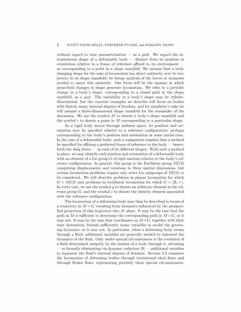
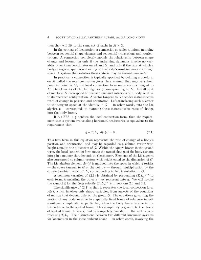
Fig. 1. A principal fiber bundle M ×G. The base manifold M is shown with twodimensions and the group G with one. A connection defines a horizontal subspace ofeach tangent space T(r,g)(M × G), isomorphic to the tangent space TrM and comple-mentary to the vertical subspace of T(r,g)(M ×G). The curve in M passing through r1has a unique horizontal lift passing through (r1, g1).

Section 3 summarizes a model in which a finite collection of point vorticesis used to represent additional degrees of freedom in the fluid surroundinga planar swimmer.

The product M ×G may be regarded as a fiber bundle over M . Eachbase point corresponds to a particular body shape; the points comprisingthe fiber over this base point represent the various ways of situating andorienting the body in its environment. Since G is a Lie group, the bundleover M is a principal bundle [7], accommodating the constructions definedbelow.

2.2. Principal Connections and Driftless Locomotion. A con-nection on the principal fiber bundle M ×G specifies a manner in which apath in M passing through the point r may be identified with a unique pathin M ×G passing through a given point in the fiber over r. A connectioncorresponds to a splitting of the tangent space at each point in M ×G intohorizontal and vertical subspaces. The horizontal subspace at each point inthe fiber over r is isomorphic to TrM . The vertical subspace has dimensionequal to the dimension of G; identifying T(r,g)(M × G) with TrM × TgGwe regard the vertical subspace as comprising vectors in TrM ×TgG of theform (0, ·). See Figure 1.

A trajectory in M ×G is said to be horizontal relative to a given con-nection if every vector tangent to the trajectory is horizontal. A horizontallift of a trajectory in M is a horizontal trajectory in M ×G that projectsonto the trajectory in M . If two trajectories in M correspond to the samepath — in other words, they differ only in their time-parameterizations —

4 SCOTT DAVID KELLY, PARTHESH PUJARI, and HAILONG XIONG

then they will lift to the same set of paths in M ×G.

In the context of locomotion, a connection specifies a unique mappingbetween sequential shape changes and sequential translations and reorien-tations. A connection completely models the relationship between shapechange and locomotion only if the underlying dynamics involve no vari-ables other than coordinates on M and G, and only if the rate at which abody changes shape has no bearing on the body’s resulting motion throughspace. A system that satisfies these criteria may be termed kinematic.

In practice, a connection is typically specified by defining a one-formon M called the local connection form. In a manner that may vary frompoint to point in M , the local connection form maps vectors tangent toM into elements of the Lie algebra g corresponding to G. Recall thatelements in G correspond to translations and rotations of a body relativeto its reference configuration. A vector tangent to G encodes instantaneousrates of change in position and orientation. Left-translating such a vectorto the tangent space at the identity in G — in other words, into the Liealgebra g — corresponds to mapping these instantaneous rates of changeinto the body frame.

If A : TM → g denotes the local connection form, then the require-ment that a system evolve along horizontal trajectories is equivalent to therequirement that

g + TeLg [A(r)r] = 0. (2.1)

This first term in this equation represents the rate of change of a body’sposition and orientation, and may be regarded as a column vector withheight equal to the dimension of G. Within the square braces in the secondterm, the local connection form maps the rate of change of the body’s shapeinto g in a manner that depends on the shape r. Elements of the Lie algebraalso correspond to column vectors with height equal to the dimension of G.The Lie algebra element A(r)r is mapped into the space in which g resides— the space tangent to G at the point g — through multiplication by thesquare Jacobian matrix TeLg corresponding to left translation in G.

A common variation of (2.1) is obtained by prepending (TeLg)−1 to

each term, translating the objects they represent into g. We will invokethe symbol ξ for the body velocity (TeLg)

−1g in Sections 2.4 and 3.2.

The significance of (2.1) is that it separates the local connection formA(r), which involves only shape variables, from aspects of the equationsof motion that depend only on the group G. The equations governing themotion of any body relative to a spatially fixed frame of reference inheritsignificant complexity, in particular, when the body frame is able to ro-tate relative to the spatial frame. This complexity is generic to the choiceof spatial frame, however, and is completely encoded in the matrix rep-resenting TeLg. The distinctions between two different kinematic systemsfor locomotion in the same ambient space — in other words, involving the

FISHLIKE SWIMMING IN A PLANAR IDEAL FLOW 5

2 4 6 8 10 12

inviscid

Stokes

ab

x

0

1

-1

0

0

0.05

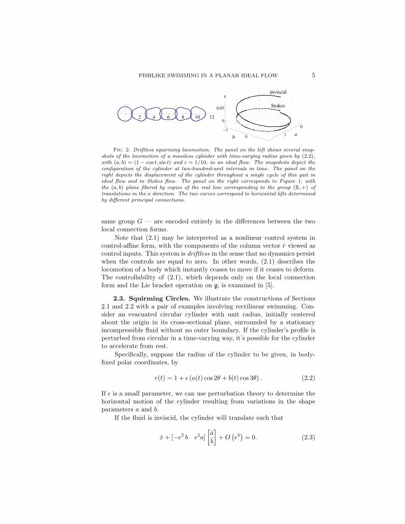
Fig. 2. Driftless squirming locomotion. The panel on the left shows several snap-shots of the locomotion of a massless cylinder with time-varying radius given by (2.2),with (a, b) = (1 − cos t, sin t) and ε = 1/10, in an ideal flow. The snapshots depict theconfiguration of the cylinder at two-hundred-unit intervals in time. The panel on theright depicts the displacement of the cylinder throughout a single cycle of this gait inideal flow and in Stokes flow. The panel on the right corresponds to Figure 1, withthe (a, b) plane fibered by copies of the real line corresponding to the group (R,+) oftranslations in the x direction. The two curves correspond to horizontal lifts determinedby different principal connections.

same group G — are encoded entirely in the differences between the twolocal connection forms.

Note that (2.1) may be interpreted as a nonlinear control system incontrol-affine form, with the components of the column vector r viewed ascontrol inputs. This system is driftless in the sense that no dynamics persistwhen the controls are equal to zero. In other words, (2.1) describes thelocomotion of a body which instantly ceases to move if it ceases to deform.The controllability of (2.1), which depends only on the local connectionform and the Lie bracket operation on g, is examined in [5].

2.3. Squirming Circles. We illustrate the constructions of Sections2.1 and 2.2 with a pair of examples involving rectilinear swimming. Con-sider an evacuated circular cylinder with unit radius, initially centeredabout the origin in its cross-sectional plane, surrounded by a stationaryincompressible fluid without no outer boundary. If the cylinder’s profile isperturbed from circular in a time-varying way, it’s possible for the cylinderto accelerate from rest.

Specifically, suppose the radius of the cylinder to be given, in body-fixed polar coordinates, by

r(t) = 1 + ε (a(t) cos 2θ + b(t) cos 3θ) . (2.2)

If ε is a small parameter, we can use perturbation theory to determine thehorizontal motion of the cylinder resulting from variations in the shapeparameters a and b.

If the fluid is inviscid, the cylinder will translate such that

x+ [−ε2 b ε2a]

[a

b

]+O

(ε3)

= 0. (2.3)

6 SCOTT DAVID KELLY, PARTHESH PUJARI, and HAILONG XIONG

Compare this equation to (2.1). The group G comprises only translationsin the x direction, and the Jacobian TeLg is the one-by-one identity ma-trix. The local connection form is represented (to order ε2) by the matrix[−ε2 b ε2a].

If Stokes flow is assumed instead of ideal flow, the cylinder will trans-late such that

x+

[ε2b

4

ε2a

2

] [a

b

]+O

(ε3)

= 0. (2.4)

Figure 2 illustrates the difference between swimming in ideal flow and swim-ming in Stokes flow with a gait that favors the former. In either case,the displacement of the cylinder after a single cyclic deformation may beregarded as the geometric phase or holonomy associated with the corre-sponding closed path in the shape manifold with coordinates a and b.

The local connection form in (2.3) encodes the fact that the Kelvinimpulse [8] in the system — effectively the total momentum — must re-main zero even after the cylinder begins to deform, requiring that certaindeformations be accompanied by translation. The conservation of impulsein the horizontal direction is equivalent, via Noether’s theorem [9], to aone-dimensional symmetry manifest in the invariance of the system’s ki-netic energy under horizontal translations of the spatial frame of reference.Formally, we derive the local connection form — following a procedureoutlined in [4] — by constructing the momentum map associated with thissymmetry. In the context of the inviscid swimmer in Figure 2, the mo-mentum map corresponds to the component of impulse in the horizontaldirection, which is related to the left-hand side of (2.3) by a nonzero mul-tiplicative factor.1 The impulse, initially zero, is conserved if and only ifthe left-hand side of (2.3) equals zero.

This procedure applies to inviscid swimming in three dimensions aswell, involving rotation as well as translation. In the most general case, thesymmetry group is all of SE(3), and the momentum map has six compo-nents corresponding to linear and angular impulse. The local connectionform in this case — taking values in se(3) — has six components as well,specifying the linear and angular velocity of the swimmer relative to thebody frame such that all components of impulse remain zero.

Significantly, the same procedure is used to derive the local connec-tion form governing locomotion in three-dimensional Stokes flow.2 In thiscase, the relevant symmetry is the invariance not of the kinetic energy butof the rate of energy dissipation — the Rayleigh dissipation function —under translations and rotations of the spatial reference frame. Specifyingthat the corresponding momentum map remain zero is equivalent to speci-fying that the net force and moment on a swimmer remain zero in the low

1Specifically, the swimmer’s effective mass in the horizontal direction.2Planar Stokes flow requires a modified treatment due to Stokes’ paradox [1].

FISHLIKE SWIMMING IN A PLANAR IDEAL FLOW 7

Reynolds number limit, consistent with the negation of inertial phenomenaby viscous effects.

2.4. Extensions to Systems with Drift. In certain cases, the no-tion of a connection on the bundle M ×G over M may assist in the math-ematical description of locomotion even when trajectories in M do not liftuniquely. Suppose, for instance, that a system is governed by Lagrange’sequations subject to viscous dissipation, and that both the Lagrangian —generalizing the role played by kinetic energy in Section 2.3 — and thedissipation function are invariant under transformations in G. In such acase, a deforming body may accumulate momentum through cyclic defor-mation, translating or rotating to different degrees during successive cycles.The position and orientation of the body evolve dynamically in a mannercoupled to the dynamics of the corresponding components of momentum.

If Amech and AStokes denote the local connection forms derived from theLagrangian and the dissipation function, respectively, then the dynamicsof the system may be expressed in the form

g = TeLg(−Amechr + I−1 p

)p = V (AStokes −Amech) r + V I−1 p+ ad∗ξ p.

(2.5)

Here p, a vector in the space g∗ dual to g, comprises the components ofthe momentum map derived from the Lagrangian — in other words, thelinear and angular momentum or impulse — expressed in the body frame.If the momentum map is conserved, its representation in the body framewill change as the body frame does; the final term in the second line tracksthis change. The local locked inertia tensor I expresses the body’s shape-dependent inertia, and V the body’s shape-dependent directional viscousresistance, in the body frame.

Observe that if V = 0 and if p = 0 initially — in other words, if alldissipation is removed from the system and the system is initially at rest— then (2.5) simplifies to (2.1) with Amech as the local connection form.The significance of inertial effects relative to viscous effects is representedby IV −1. Prepending this tensor term-by-term to the second line in (2.5)and letting IV −1 → 0, we recover (2.1) with AStokes as the local connectionform.3

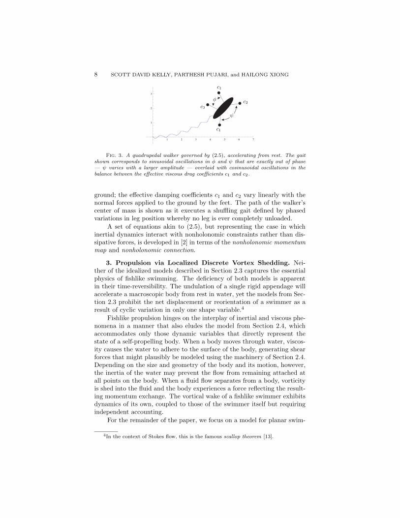
Figure 3 depicts a system described by equations of the form (2.5). Asimple walker with a uniformly dense elliptical body makes contact with theground at four points, each at the end of a rigidly pivoting leg. The angles φand ψ specify the shape of the walker as viewed from above. An additionalparameter, representing the walker’s ability to lift its legs in opposite pairs,specifies the distribution of the walker’s weight on its four feet. Each footis assumed to experience isotropic viscous resistance to sliding along the

3Compare the role of of IV −1 here to that of the Reynolds number in the Navier-Stokes equations, which become the equations for creeping flow as Re→ 0 [3].

8 SCOTT DAVID KELLY, PARTHESH PUJARI, and HAILONG XIONG

1 2 3 4 5 6 7

1

2

3

φ

ψ

c1

c1

c2c2

Fig. 3. A quadrupedal walker governed by (2.5), accelerating from rest. The gaitshown corresponds to sinusoidal oscillations in φ and ψ that are exactly out of phase— ψ varies with a larger amplitude — overlaid with cosinusoidal oscillations in thebalance between the effective viscous drag coefficients c1 and c2.

ground; the effective damping coefficients c1 and c2 vary linearly with thenormal forces applied to the ground by the feet. The path of the walker’scenter of mass is shown as it executes a shuffling gait defined by phasedvariations in leg position whereby no leg is ever completely unloaded.

A set of equations akin to (2.5), but representing the case in whichinertial dynamics interact with nonholonomic constraints rather than dis-sipative forces, is developed in [2] in terms of the nonholonomic momentummap and nonholonomic connection.

3. Propulsion via Localized Discrete Vortex Shedding. Nei-ther of the idealized models described in Section 2.3 captures the essentialphysics of fishlike swimming. The deficiency of both models is apparentin their time-reversibility. The undulation of a single rigid appendage willaccelerate a macroscopic body from rest in water, yet the models from Sec-tion 2.3 prohibit the net displacement or reorientation of a swimmer as aresult of cyclic variation in only one shape variable.4

Fishlike propulsion hinges on the interplay of inertial and viscous phe-nomena in a manner that also eludes the model from Section 2.4, whichaccommodates only those dynamic variables that directly represent thestate of a self-propelling body. When a body moves through water, viscos-ity causes the water to adhere to the surface of the body, generating shearforces that might plausibly be modeled using the machinery of Section 2.4.Depending on the size and geometry of the body and its motion, however,the inertia of the water may prevent the flow from remaining attached atall points on the body. When a fluid flow separates from a body, vorticityis shed into the fluid and the body experiences a force reflecting the result-ing momentum exchange. The vortical wake of a fishlike swimmer exhibitsdynamics of its own, coupled to those of the swimmer itself but requiringindependent accounting.

For the remainder of the paper, we focus on a model for planar swim-

4In the context of Stokes flow, this is the famous scallop theorem [13].

FISHLIKE SWIMMING IN A PLANAR IDEAL FLOW 9

-2 -1 1 2

-1.0

-0.5

0.5

1.0

-2 -1 1 2

-1.0

-0.5

0.5

1.0

-2 -1 1 2

-1.0

-0.5

0.5

1.0

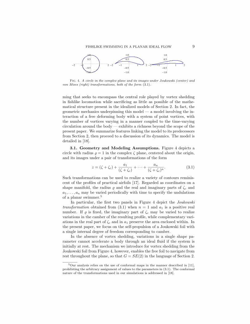
Fig. 4. A circle in the complex plane and its images under Joukowski (center) andvon Mises (right) transformations, both of the form (3.1).

ming that seeks to encompass the central role played by vortex sheddingin fishlike locomotion while sacrificing as little as possible of the mathe-matical structure present in the idealized models of Section 2. In fact, thegeometric mechanics underpinning this model — a model involving the in-teraction of a free deforming body with a system of point vortices, withthe number of vortices varying in a manner coupled to the time-varyingcirculation around the body — exhibits a richness beyond the scope of thepresent paper. We summarize features linking the model to its predecessorsfrom Section 2, then proceed to a discussion of its dynamics. The model isdetailed in [18].

3.1. Geometry and Modeling Assumptions. Figure 4 depicts acircle with radius % = 1 in the complex ζ plane, centered about the origin,and its images under a pair of transformations of the form

z = (ζ + ζc) +a1

(ζ + ζc)+ · · ·+ an

(ζ + ζc)n. (3.1)

Such transformations can be used to realize a variety of contours reminis-cent of the profiles of practical airfoils [17]. Regarded as coordinates on ashape manifold, the radius % and the real and imaginary parts of ζc anda1, . . . , an may be varied periodically with time to specify the undulationsof a planar swimmer.5

In particular, the first two panels in Figure 4 depict the Joukowskitransformation obtained from (3.1) when n = 1 and a1 is a positive realnumber. If % is fixed, the imaginary part of ζc may be varied to realizevariations in the camber of the resulting profile, while complementary vari-ations in the real part of ζc and in a1 preserve the area enclosed within. Inthe present paper, we focus on the self-propulsion of a Joukowski foil witha single internal degree of freedom corresponding to camber.

In the absence of vortex shedding, variations in a single shape pa-rameter cannot accelerate a body through an ideal fluid if the system isinitially at rest. The mechanism we introduce for vortex shedding from theJoukowski foil from Figure 4, however, enables the free foil to navigate fromrest throughout the plane, so that G = SE(2) in the language of Section 2.

5Our analysis relies on the use of conformal maps in the manner described in [11],prohibiting the arbitrary assignment of values to the parameters in (3.1). The conformalnature of the transformations used in our simulations is addressed in [18].

10 SCOTT DAVID KELLY, PARTHESH PUJARI, and HAILONG XIONG

The body frame is affixed to the deforming foil so that its coordinate axescoincide with the real and imaginary axes of the complex plane in whichthe foil’s shape is obtained from the Joukowski map.

Adopting the perspective of [16] and significant subsequent literature,we focus on vortex shedding from the sharp trailing tip of the foil — mod-eling the caudal fin of a fish viewed in cross-section — as a mechanismfor propulsion. We assume the fluid surrounding the foil to be ideal, andconfine the representation of viscous phenomenology to the time-periodicenforcement of a Kutta condition [3] at this single point.

The Kutta condition compels smooth flow separation from the foil’strailing tip by requiring that the preimage of the tip in the ζ plane corre-spond to a stagnation point for the preimage of the flow. This conditioncan be enforced continuously through the continuous introduction of vor-ticity to the fluid, but we amend the flow only at regular instants in timeby introducing discrete vortices near the foil’s tip. Given the freedom tochoose both the location and the strength of a newly introduced vortex,we can enforce the Kutta condition in more than one way. The simulationsdepicted below rely on a method adapted from [15] whereby the locationof each new vortex is specified before its strength, and shed vortices neednot have the same strength. A comparison of alternate methods appearsin [18]. Once shed, each vortex in our model remains constant in strength.

New vortices are introduced to the fluid in a manner that respects twoconservation laws, each of which can be traced to a symmetry of the fluid-foil system. Consistent with Kelvin’s circulation theorem [3], the circulationaround the foil changes discretely with the shedding of each new vortexto ensure that the circulation around any contour enclosing the foil andits wake remain zero. Changes in the circulation around the foil may beattributed to the introduction of image vortices [11] within the foil. Therelationship between Kelvin’s theorem and the invariance of kinetic energyunder fluid particle relabeling is discussed in [10].

Consistent with the conservation of total impulse in the system, thelinear and angular momenta of the foil must also change discretely withthe introduction of each new vortex. Note that changes in the foil’s veloc-ity affect the fluid velocity, requiring the simultaneous application of theconstraints imposed on shed vortex strength and placement by the Kuttacondition and by impulse conservation.

3.2. Hamiltonian Structure. The interaction of a free solid bodywith a finite collection of point vortices in an infinite ideal fluid is governedby a system of ordinary differential equations exhibiting a non-canonicalHamiltonian structure. This is demonstrated in [14] for the case in whichthe body is rigid. We summarize the extension in [18] to the case in whichthe body deforms as the image of a circle with radius %, centered aboutthe origin in the complex ζ plane, under a time-varying transformationz = F (ζ). We assume z = F (ζ) to be parametrized by coordinates rj

FISHLIKE SWIMMING IN A PLANAR IDEAL FLOW 11

on the appropriate shape manifold. Between vortex-shedding events, theswimming foil in our model interacts with ambient vortices — whether pre-viously shed by the foil or present initially — according to these equations.

The phase space in question is the product of g∗ — elements p in whichencode the linear and angular impluse in the system — and the space ofcoordinate pairs (xi, yi) specifying the positions of the vortices relative tothe body frame. If n denotes the total number of vortices at a given timeand γi the strength of the ith vortex, we may define a Hamiltonian of theform

H(p, x1, y1, . . . , xn, yn) = H0 − 2πH1 (3.2)

relative to which the fluid impulse evolves according to the Lie-Poissonequation

p = ad∗δH/δp p

and the positions of the vortices evolve according to the equations

−2πγixi =∂H

∂yi, −2πγiyi = −∂H

∂xi.

The significance of the Lie-Poisson equation in Hamiltonian mechanics isdetailed in [9].

While expressible in terms of the phase variables named above, thefirst term in the Hamiltonian (3.2) is most easily understood as

H0 =1

2ξT Iξ,

where ξ and I are the body velocity vector and locked inertia tensor fromSection 2. The second term in the Hamiltonian is proportional to

H1 =∑i

γi∑j

rjψj(xi, yi)−1

2

∑i

γ2i(log∣∣ζiζi − %2∣∣+ log |F ′(ζi)|

)+

1

2

∑i

∑i 6=j

γiγj(log |ζi − ζj | − log

∣∣ζk ζj − %2∣∣) ,where ζi denotes the preimage of the location of the ith vortex in the ζplane and rjψj is the component of the stream function in the ζ plane dueto variations in the shape parameter rj .

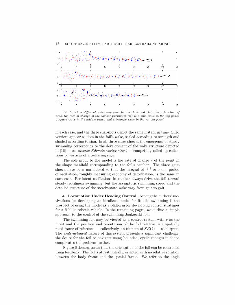
3.3. Steady Swimming. Vortex shedding from the trailing tip ofa free Joukowski foil serves to rectify oscillations in the foil’s camber togenerate locomotion. Figure 5 depicts snapshots from simulations of threedifferent swimming gaits corresponding to different cyclic variations in cam-ber over time. The foil begins at rest and oscillates at the same frequency

12 SCOTT DAVID KELLY, PARTHESH PUJARI, and HAILONG XIONG

Fig. 5. Three different swimming gaits for the Joukowski foil. As a function oftime, the rate of change of the camber parameter r(t) is a sine wave in the top panel,a square wave in the middle panel, and a triangle wave in the bottom panel.

in each case, and the three snapshots depict the same instant in time. Shedvortices appear as dots in the foil’s wake, scaled according to strength andshaded according to sign. In all three cases shown, the emergence of steadyswimming corresponds to the development of the wake structure depictedin [16] — an inverse Karman vortex street — comprising rolled-up collec-tions of vortices of alternating sign.

The sole input to the model is the rate of change r of the point inthe shape manifold corresponding to the foil’s camber. The three gaitsshown have been normalized so that the integral of |r|2 over one periodof oscillation, roughly measuring economy of deformation, is the same ineach case. Persistent oscillations in camber always drive the foil towardsteady rectilinear swimming, but the asymptotic swimming speed and thedetailed structure of the steady-state wake vary from gait to gait.

4. Locomotion Under Heading Control. Among the authors’ mo-tivations for developing an idealized model for fishlike swimming is theprospect of using the model as a platform for developing control strategiesfor a fishlike robotic vehicle. In the remaining pages, we outline a simpleapproach to the control of the swimming Joukowski foil.

The swimming foil may be viewed as a control system with r as theinput and the position and orientation of the foil relative to a spatiallyfixed frame of reference — collectively, an element of SE(2) — as outputs.The underactuated nature of this system presents a significant challenge;the desire for the foil to navigate using bounded, cyclic changes in shapecomplicates the problem further.

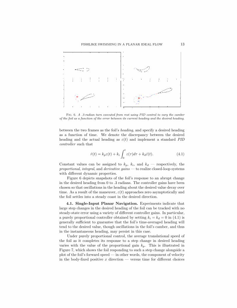
Figure 6 demonstrates that the orientation of the foil can be controlledusing feedback. The foil is at rest initially, oriented with no relative rotationbetween the body frame and the spatial frame. We refer to the angle

FISHLIKE SWIMMING IN A PLANAR IDEAL FLOW 13

Fig. 6. A .3-radian turn executed from rest using PID control to vary the camberof the foil as a function of the error between its current heading and the desired heading.

between the two frames as the foil’s heading, and specify a desired headingas a function of time. We denote the discrepancy between the desiredheading and the actual heading as ε(t) and implement a standard PIDcontroller such that

r(t) = kpε(t) + ki

∫ t

0

ε(τ)dτ + kdε(t). (4.1)

Constant values can be assigned to kp, ki, and kd — respectively, theproportional, integral, and derivative gains — to realize closed-loop systemswith different dynamic properties.

Figure 6 depicts snapshots of the foil’s response to an abrupt changein the desired heading from 0 to .3 radians. The controller gains have beenchosen so that oscillations in the heading about the desired value decay overtime. As a result of the maneuver, ε(t) approaches zero asymptotically andthe foil settles into a steady coast in the desired direction.

4.1. Single-Input Planar Navigation. Experiments indicate thatlarge step changes in the desired heading of the foil can be tracked with nosteady-state error using a variety of different controller gains. In particular,a purely proportional controller obtained by setting ki = kd = 0 in (4.1) isgenerally sufficient to guarantee that the foil’s time-averaged heading willtend to the desired value, though oscillations in the foil’s camber, and thusin the instantaneous heading, may persist in this case.

Under purely proportional control, the average translational speed ofthe foil as it completes its response to a step change in desired headingvaries with the value of the proportional gain kp. This is illustrated inFigure 7, which shows the foil responding to such a step change alongside aplot of the foil’s forward speed — in other words, the component of velocityin the body-fixed positive x direction — versus time for different choices

14 SCOTT DAVID KELLY, PARTHESH PUJARI, and HAILONG XIONG

longitudinal

velocity

time

kp = 8

kp = 12

Fig. 7. Left: A directional change under proportional heading control, leading tosteady average translation at a speed determined by the proportional gain kp. Right:The longitudinal velocity of the foil as it executes such a maneuver, as a function oftime, for two different values of kp.

of kp. The foil begins not at rest but coasting steadily from left to right,parallel with the bottom of the figure.

Proportional heading control thus forms the basis for a simple methodwhereby the foil can navigate throughout the plane. Desired changes inswimming direction are achieved through feedback between heading andcamber; changes in the steady-state swimming speed are achieved throughchanges in the feedback gain.

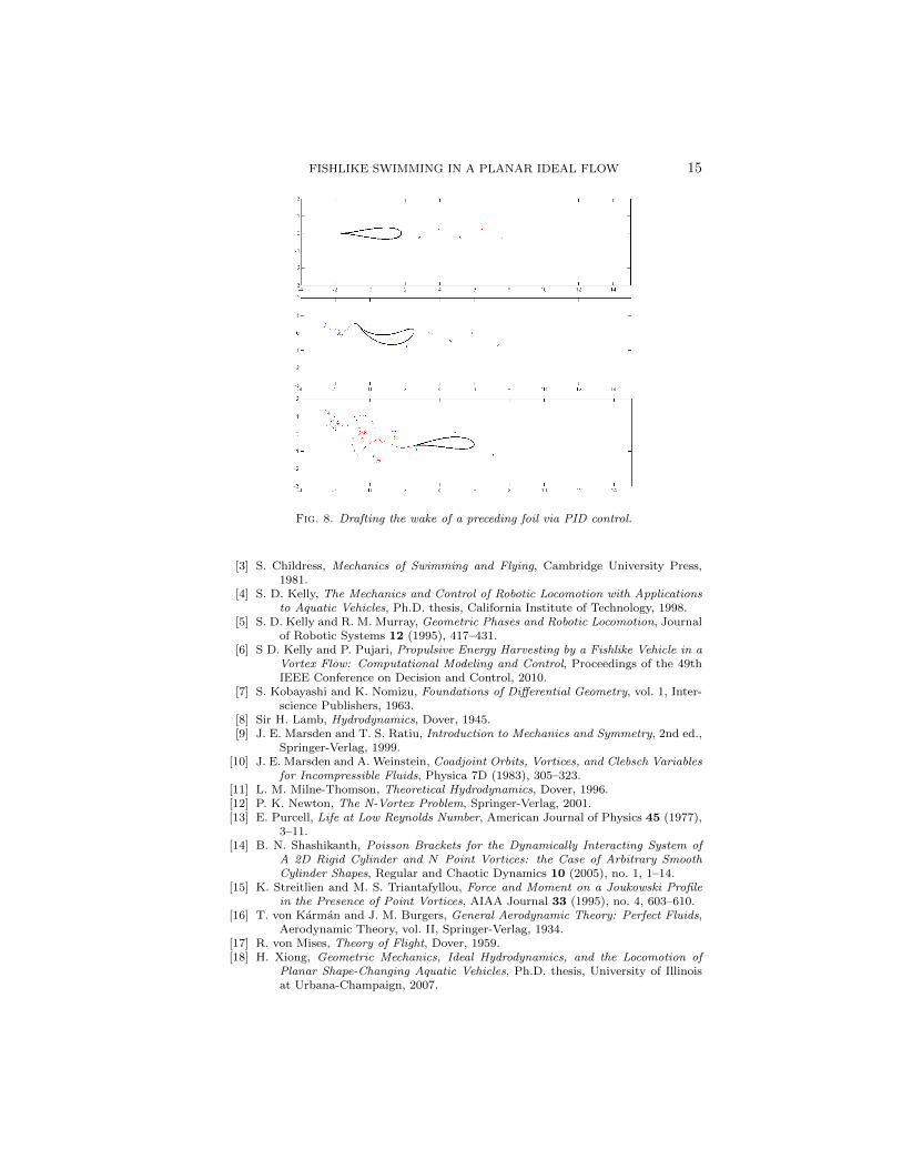
4.2. Energy Harvesting. A nonzero background flow can compli-cate the variations in camber required for the foil to track a desired head-ing, but need not increase the control effort required to attain a desiredheading and asymptotic speed. Figure 8 illustrates the use of PID controlfor energy harvesting from an array of vortices corresponding to the fullyrolled-up wake of a foil executing the sinusoidal gait from Figure 5.

The controller gains are chosen to damp oscillations in the foil’s camberand the desired heading remains equal to the foil’s initial heading. As theambient vortices begin to rotate the foil, it responds in a manner that sta-bilizes its motion through the middle of the street. Without deformation,the foil would be ejected laterally [6]. With control, it attains a transla-tional kinetic energy greater than that achievable with the same economyof deformation in a quiescent fluid, while the total interaction energy [12]among vortices decreases.

REFERENCES

[1] G. Birkhoff, Hydrodynamics: A Study in Logic, Fact, and Similitude, GreenwoodPublishing Group, 1978.

[2] A. M. Bloch, P. S. Krishnaprasad, J. E. Marsden, and R. M. Murray, Nonholo-nomic Mechanical Systems with Symmetry, Archive for Rational Mechanicsand Analysis 136 (1996), 21–99.

FISHLIKE SWIMMING IN A PLANAR IDEAL FLOW 15

Fig. 8. Drafting the wake of a preceding foil via PID control.

[3] S. Childress, Mechanics of Swimming and Flying, Cambridge University Press,1981.

[4] S. D. Kelly, The Mechanics and Control of Robotic Locomotion with Applicationsto Aquatic Vehicles, Ph.D. thesis, California Institute of Technology, 1998.

[5] S. D. Kelly and R. M. Murray, Geometric Phases and Robotic Locomotion, Journalof Robotic Systems 12 (1995), 417–431.

[6] S D. Kelly and P. Pujari, Propulsive Energy Harvesting by a Fishlike Vehicle in aVortex Flow: Computational Modeling and Control, Proceedings of the 49thIEEE Conference on Decision and Control, 2010.

[7] S. Kobayashi and K. Nomizu, Foundations of Differential Geometry, vol. 1, Inter-science Publishers, 1963.

[8] Sir H. Lamb, Hydrodynamics, Dover, 1945.[9] J. E. Marsden and T. S. Ratiu, Introduction to Mechanics and Symmetry, 2nd ed.,

Springer-Verlag, 1999.[10] J. E. Marsden and A. Weinstein, Coadjoint Orbits, Vortices, and Clebsch Variables

for Incompressible Fluids, Physica 7D (1983), 305–323.[11] L. M. Milne-Thomson, Theoretical Hydrodynamics, Dover, 1996.[12] P. K. Newton, The N-Vortex Problem, Springer-Verlag, 2001.[13] E. Purcell, Life at Low Reynolds Number, American Journal of Physics 45 (1977),

3–11.[14] B. N. Shashikanth, Poisson Brackets for the Dynamically Interacting System of

A 2D Rigid Cylinder and N Point Vortices: the Case of Arbitrary SmoothCylinder Shapes, Regular and Chaotic Dynamics 10 (2005), no. 1, 1–14.

[15] K. Streitlien and M. S. Triantafyllou, Force and Moment on a Joukowski Profilein the Presence of Point Vortices, AIAA Journal 33 (1995), no. 4, 603–610.

[16] T. von Karman and J. M. Burgers, General Aerodynamic Theory: Perfect Fluids,Aerodynamic Theory, vol. II, Springer-Verlag, 1934.

[17] R. von Mises, Theory of Flight, Dover, 1959.[18] H. Xiong, Geometric Mechanics, Ideal Hydrodynamics, and the Locomotion of

Planar Shape-Changing Aquatic Vehicles, Ph.D. thesis, University of Illinoisat Urbana-Champaign, 2007.