Symplectic Topology and Geometric Quantum Mechanics

by

Barbara Sanborn

A Dissertation Presented in Partial Fulfillmentof the Requirements for the Degree

Doctor of Philosophy

Approved July 2011 by theGraduate Supervisory Committee:

Sergei Suslov, ChairDonald Jones

Jose MenendezJohn Quigg

John Spielberg

ARIZONA STATE UNIVERSITY

August 2011

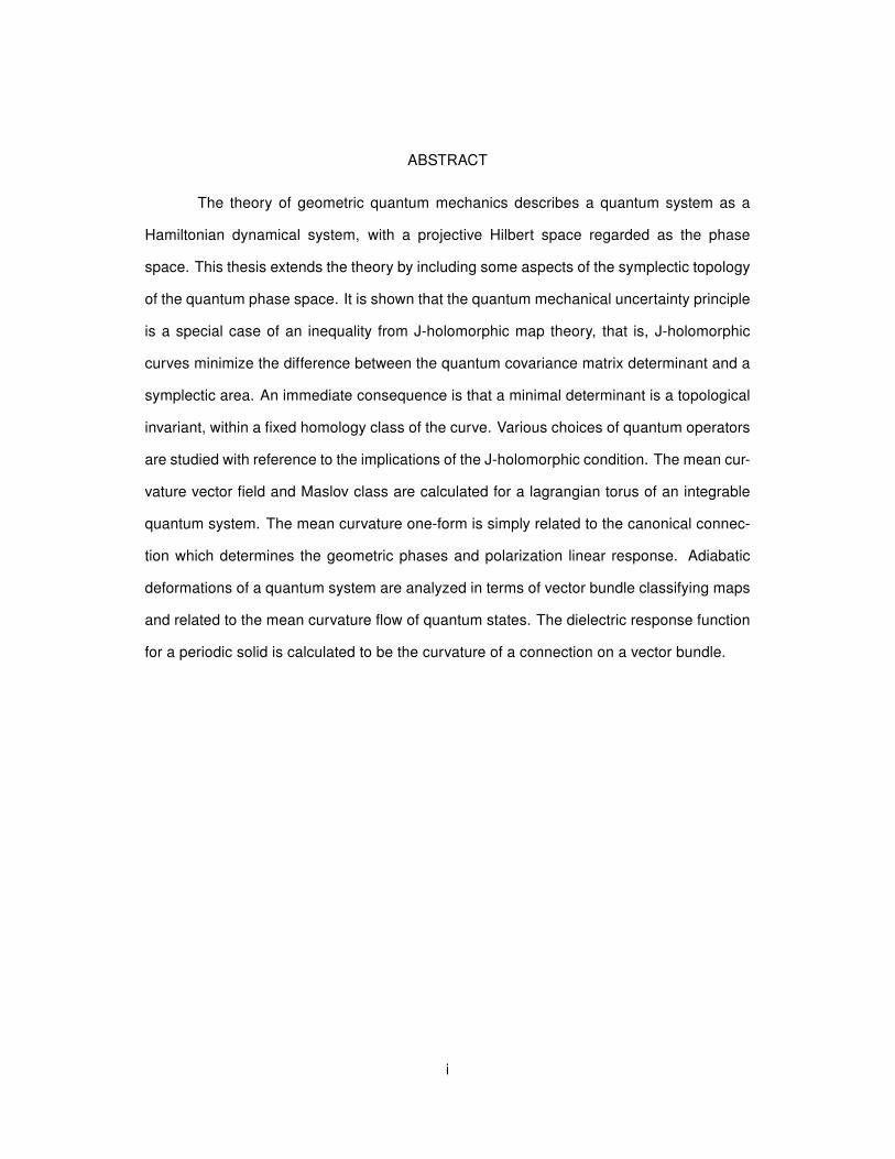
ABSTRACT

The theory of geometric quantum mechanics describes a quantum system as a

Hamiltonian dynamical system, with a projective Hilbert space regarded as the phase

space. This thesis extends the theory by including some aspects of the symplectic topology

of the quantum phase space. It is shown that the quantum mechanical uncertainty principle

is a special case of an inequality from J-holomorphic map theory, that is, J-holomorphic

curves minimize the difference between the quantum covariance matrix determinant and a

symplectic area. An immediate consequence is that a minimal determinant is a topological

invariant, within a fixed homology class of the curve. Various choices of quantum operators

are studied with reference to the implications of the J-holomorphic condition. The mean cur-

vature vector field and Maslov class are calculated for a lagrangian torus of an integrable

quantum system. The mean curvature one-form is simply related to the canonical connec-

tion which determines the geometric phases and polarization linear response. Adiabatic

deformations of a quantum system are analyzed in terms of vector bundle classifying maps

and related to the mean curvature flow of quantum states. The dielectric response function

for a periodic solid is calculated to be the curvature of a connection on a vector bundle.

i

TABLE OF CONTENTS

Page

TABLE OF CONTENTS . . . . . . . . . . . . . . . . . . . . . . . . . . . . . . . . . ii

CHAPTER . . . . . . . . . . . . . . . . . . . . . . . . . . . . . . . . . . . . . . . . . 1

1 INTRODUCTION . . . . . . . . . . . . . . . . . . . . . . . . . . . . . . . . . . . 1

2 A GEOMETRIC VIEW OF QUANTUM MECHANICS . . . . . . . . . . . . . . . . 6

2.1 Hamiltonian Dynamics . . . . . . . . . . . . . . . . . . . . . . . . . . . . . 6

2.2 Quantum Mechanics as a Hamiltonian Dynamical System . . . . . . . . . . 9

2.3 The Uncertainty Principle in Terms of the Kähler Structure . . . . . . . . . . 13

2.4 The Role of the Principal Connection . . . . . . . . . . . . . . . . . . . . . 16

2.5 Quantum Mechanics as an Integrable System . . . . . . . . . . . . . . . . 21

3 J-HOLOMORPHIC MAPS AND THE UNCERTAINTY PRINCIPLE . . . . . . . . . 24

3.1 Introduction . . . . . . . . . . . . . . . . . . . . . . . . . . . . . . . . . . . 24

3.2 The Covariance Matrix Determinant . . . . . . . . . . . . . . . . . . . . . . 25

3.3 J -Holomorphic Maps . . . . . . . . . . . . . . . . . . . . . . . . . . . . . . 26

3.4 Minimal Uncertainty and the Holomorphic Condition . . . . . . . . . . . . . 28

3.5 Examples . . . . . . . . . . . . . . . . . . . . . . . . . . . . . . . . . . . . 31

4 DEFORMATIONS OF A QUANTUM SYSTEM . . . . . . . . . . . . . . . . . . . . 35

4.1 Symplectic and Hamiltonian Deformations . . . . . . . . . . . . . . . . . . 35

4.2 Mean Curvature and the Maslov Class . . . . . . . . . . . . . . . . . . . . 38

4.3 Berry’s Phase and Mean Curvature Flow . . . . . . . . . . . . . . . . . . . 41

4.4 The Vector Bundle Classification Theorem . . . . . . . . . . . . . . . . . . 45

4.5 The Adiabatic Theorem . . . . . . . . . . . . . . . . . . . . . . . . . . . . . 49

5 ADIABATIC CURVATURE AND THE RESPONSE OF A CRYSTALLINE SOLID . 55

5.1 Symplectic Structure of the Periodic Solid . . . . . . . . . . . . . . . . . . . 55

5.2 The Spectral Bundle and the One-Band Subbundle . . . . . . . . . . . . . 57

5.3 The Current-Current Correlation Function . . . . . . . . . . . . . . . . . . . 61

6 FUNDAMENTALS AND EXAMPLES . . . . . . . . . . . . . . . . . . . . . . . . . 65

6.1 Vector Fields, Lie Groups, and Homogeneous Spaces . . . . . . . . . . . . 65ii

Chapter Page

6.2 Principal Bundles and Connections . . . . . . . . . . . . . . . . . . . . . . 72

6.3 Horizontal Lifts and Holonomy . . . . . . . . . . . . . . . . . . . . . . . . . 76

6.4 Associated Bundles and the Covariant Derivative . . . . . . . . . . . . . . . 81

6.5 Metrics, Symplectic Manifolds, and Hamiltonian Vector Fields . . . . . . . . 83

REFERENCES . . . . . . . . . . . . . . . . . . . . . . . . . . . . . . . . . . . . . . 89

iii

Chapter 1

INTRODUCTION

The primary objective of this thesis is to describe an approach to quantum mechanics that is

based in a framework of differential geometry and Hamiltonian dynamical systems. Topol-

ogy and geometry of symplectic manifolds are fundamental to this approach. The guiding

purpose of the thesis is to formulate a geometric description of condensed matter physics

by application of geometric quantum mechanics to many-body systems. The project was

originally motivated by developments in condensed matter physics that involve a geometric

perspective on the electronic properties of matter, particularly where holonomy and charac-

teristic classes arise. An important feature to understand in this perspective is the geometric

phase appearing in theories of the polarization and transport properties of matter.[95, 82]

According to the modern theory of polarization,[82, 88] the information about the macro-

scopic polarization of an extended insulating system such as a periodic crystalline solid, is

not in the charge density, but in the wave function. Also related to the geometric underpin-

nings of our understanding of interactions in matter, is pre-metric electromagnetism which

features the significance of the constitutive relation.[47, 46, 35, 36]

During the same period of time that intrinsic geometric structures of matter have

been recognized in physics, a new field of mathematics has emerged: symplectic topology,

which is the study of the global structure of a symplectic manifold.[62] A foundational re-

sult is Gromov’s[43] nonsqueezing theorem, which states that if there is an embedding

of the closed symplectic Euclidean ball B2n(r) of radius r into the symplectic cylinder

B2(R)×R2n−2 that preserves the symplectic form, then r ≤ R. It shows that there is a ba-

sic property of the ball and the cylinder that is invariant under symplectomorphisms, which

is two-dimensional. The symplectic capacities[50, 62] are defined to describe this symplec-

tic area invariance. New methods have been developed to study the group of symplec-

tomorphisms of a symplectic manifold, and its relation to the group of volume-preserving

diffeomorphisms. The method of J -holomorphic curves, introduced by Gromov[43], has

proved to be an especially powerful and useful tool.1

The importance of symplectic geometry as a key to understanding the dynamics of

physical systems is well established.[6, 61] Could the new insights and methods of symplec-

tic topology be applied to the recent physical theories of matter that emphasize a synthesis

of topological and geometric perspectives? This question, and the attempt to answer it,

permeate the present work.

Quantum mechanics has traditionally been considered from an algebraic point of

view. In this view, a quantum system is described with a complex separable Hilbert space

H. The observables, or measurable quantities of the system, are represented by self-adjoint

linear operators on H, while the dynamics of the system is given by a family of unitary op-

erators. In contrast, classical mechanics is often described within a geometric perspective.

The states of a classical mechanical system are elements of a symplectic manifold, Mcl,

called the phase space of the system. The classical observables are functions on Mcl,

while the dynamics is governed by the symplectic form and a preferred Hamiltonian vector

field on Mcl. The counterintuitive observation that such a nonlinear description of me-

chanics arises in the classical approximation to purely linear interactions within the more

accurate quantum theory has prompted investigations into a more unified geometric view

of mechanics; one of the goals of such an approach is to clarify the relationship between

the classical and quantum theories. This approach has come to be known as geometric

quantum mechanics. Its foundations were laid in early work by Chernoff and Marsden[24]

and by Kibble[55] and was developed by others[8, 22, 13, 28, 48, 61, 83].

These investigations resulted in a geometric view of quantum mechanics that shows

it to be a Hamiltonian dynamical system on a symplectic manifold; the phase space is the

projective Hilbert space, P (H). Schrödinger’s equation on P (H) is equivalent to Hamilton’s

equations, determined by the natural symplectic structure arising from the Hermitian scalar

product on H. The geometric point of view emphasizes that the quantum phase space is

endowed with an extra structure not found in classical mechanics. The Kähler structure of

P (H) furnishes the space of quantum states with a Riemannian metric in addition to the

symplectic structure characteristic of Hamiltonian mechanics. This additional structure can

2

be viewed as the source of features in the quantum theory that are distinctly different from

classical mechanics.

One of the aims of geometric quantum theory has been to describe a quantum sys-

tem entirely on the Kähler manifold P (H) ∼= CP∞ without resource to the Hilbert space

H at all, and this effort has been largely successful. On the other hand, it is commonly

known that macroscopic quantum effects can arise as manifestations of the geometric

phase, which is the holonomy of a closed path in the space of states P (H). The rela-

tionship of vectors in H to quantum states in P (H) can be viewed in terms of the principal

bundle U(1) → S(H) → P (H), where S(H) = ψ ∈ H : |ψ|2 = 1. A distinguished

connection on this bundle defines the horizontal subspace of the tangent space Tψ(H) at

a point ψ ∈ H to be the orthogonal complement to the fiber at [ψ] ∈ P (H), where or-

thogonality is determined by the given Hermitian scalar product on H. The curvature of

this connection is directly related to the symplectic form Ω on P (H) which is determined

as the imaginary part of the Fubini-Study Hermitian metric. The cohomology information

contained in the expanded view which includes this extra bundle structure is somehow em-

bodied in the special structure of the quantum phase space as a homogeneous (Hermitian

symmetric) space.

An aspect of the special structure of quantum mechanics is evident in the following

notable feature. A dynamical system on P (H) determined by a time-independent Hamil-

tonian function is completely integrable. In the finite-dimensional case, the expectation

values of the eigenspace projection operators Pj are n constants of the motion. This fact

is equivalent to the existence of a torus action on P (H), providing a foliation of the quan-

tum phase space by tori L = Tn ⊂ P (H) with the lagrangian property that the symplectic

form vanishes on L, that is, Ω|L = 0. Moreover, if we define a certain symplectic vector

bundle π : E → P (H), the Lagrangian subbundle LE → P (H) is a flat bundle, that is, the

curvature of the connection vanishes on LE .

The space Λ(L) of lagrangian submanifolds of P (H) may be associated with a

family of integrable systems. Moreover, the dynamics determined by a Hamiltonian function

3

on P (H) that depends adiabatically on time can be viewed as a path in Λ(L).

The mean curvature vector field Hi of an immersion i : L → M of a lagrangian

submanifoldL inM is the trace of the second fundamental form ofL. As such, it is a section

of the normal bundle to L inM, and generates a local flow on L. A family of submanifolds

evolves under mean curvature flow if the velocity at each point of the submanifold is given by

the mean curvature vector at that point. In addition, the mean curvature one-form αHi :=

1π ιHiΩ represents the Maslov class µ ∈ H1(L,Z).[64] Since the quantum phase space

P (H) is Einstein-Kähler, the one form αHi on L = Tn ⊂ P (H) is closed[31], and so

defines a real cohomology class in H1(L,R). In particular, this means that lagrangian

submanifolds stay lagrangian under the mean curvature flow on P (H). Moreover, in this

case, under global Hamiltonian isotopy, the one forms αHi represent the same cohomology

class.

A central theme of the thesis is the study of deformations of a quantum system; one

type of such a deformation is time evolution. The investigation proceeds within an extended

framework for geometric quantum mechanics that incorporates some recent developments

in the emerging field of symplectic topology, which allows clarification of the relationship

between the notions of symplectic capacitance, the geometric phase, and the uncertainty

principle.

Chapter 2 provides a review of the theory of geometric quantum mechanics. Chap-

ter 3 shows that the quantum mechanical uncertainty principle is a special case of an in-

equality from J -holomorphic map theory. The inequality can be viewed as a comparison of

metric and symplectic areas. It is shown that the quantum covariance matrix determinant

D(A, B, z) = (∆A)2z (∆B)2

z − (C(A, B)z)2 is equal to the harmonic energy of a complex

map u : Σ → H. Moreover, J -holomorphic curves minimize the difference between the

quantum covariance matrix determinant D(A, B, z) and the square of the symplectic area

Ω(Az, Bz). When equality is achieved, the off-diagonal part C(A, B)z of the covariance

matrix vanishes and the product of the variances (∆A)z (∆B)z is a topological invariant,

within a fixed homology class of the curve. Among the examples considered is the choice

4

of A = X and B = P , the position and momentum operators. In this case, Ω(Az, Bz) = ~

represents a symplectic area in the quantum phase space.

In Chapter 4, the mean curvature vector field is calculated for a finite dimensional

quantum system, viewed as a Hamiltonian dynamical system on P (H), the Maslov class

representative is thereby determined and related to the connection one form and holonomy

group on U(1) → S(H) → P (H). Of interest is the time evolution problem determined by

the mean curvature flow of the quantum system. If the initial state is a lagrangian immer-

sion, then the closedness of the mean curvature form guarantees that the deformation is

lagrangian; that is, the mean curvature flow may be regarded as a smooth family of inte-

grable systems. The relationship between adiabatic time evolution and the mean curvature

flow of a quantum system is studied and compared to the isodrastic condition of stationary

action given by Weinstein [93].

In Chapter 5, a study of the symplectic structure of a periodic solid is begun, and

the dielectric function for a periodic solid is calculated to be the curvature of a connection

on a vector bundle. Chapter 6 serves as an appendix to provide fundamentals of differential

and symplectic geometry and includes the numbered examples.

5

Chapter 2

A GEOMETRIC VIEW OF QUANTUM MECHANICS

2.1 Hamiltonian Dynamics

A Hamiltonian dynamical system consists of a phase space, which is a smooth manifoldM

equipped with a symplectic form, and a Hamiltonian vector field XE :M→ T (M).

Recall that a two-form ω onM is symplectic if ω is closed and nondegenerate. That

is, 1) dω = 0 and 2) for each p ∈ M, ω : Tp(M) × Tp(M) → R such that ω(u, v) = 0 for

all v ∈ TpM only when u = 0.

Nondegeneracy of ω implies that the contraction map of a vector field X ∈ X(M)

with ω

ι : Tp(M)→ T ∗p (M) X 7→ ιXω defined by ιX(·) = ω(X, ·) (2.1)

is injective.

A vector field X on M is called symplectic if ιXω is closed. A vector field X on

M is called hamiltonian if iXω is exact. Equivalently, a vector field X : M → T (M) is

hamiltonian if there is a C1 function E :M→ R such that

ιXω = dE . (2.2)

Locally on every contractible open set, every symplectic vector field is hamiltonian. If the

first de Rham cohomology group is trivial, then globally every symplectic vector field is

hamiltonian. When (2.2) holds, we write X = XE and call E an energy function for the

vector field XE . (M, ω,XE) is called a Hamiltonian system.

A hamiltonian vector field XF generates the one-parameter group of diffeomor-

phisms φFt : R×M→M, where φFt ∈ DiffM satisfies ddtφ

Ft = XF φFt , φF0 = id. In

addition, as a one-parameter group φFt satisfies the flow property

φFt+s(p) = φFt (φFs (p)) for all t, s ∈ R and p ∈M . (2.3)

6

Now consider the dynamics of the Hamiltonian system (M, ω,XE). Each point

of the symplectic manifold M corresponds to a state of the system, and M is called the

state space or the phase space. The observables, or measurable quantities, in Hamiltonian

mechanics are real-valued functions onM. Any function G : M → M is constant along

the orbits of the flow of XF if and only if the Poisson bracket

G,Fz := ωz(XG, XF ) = dG(XF )(z) (2.4)

vanishes for all z ∈M.

We assume that, with respect to a given choice of time axis, the time evolution

of each state can be represented by a path in M. Let m ∈ M and let t 7→ φt be the

local 1-parameter group generated by the vector field XE in a neighborhood of m. If the

initial state is m, then the state follows the orbit zm : R → M defined by zm(t) = φt(m)

with zm(0) = m. When M is compact, the path zm is an integral curve of XE starting

at m. In other words, given the Hamiltonian vector field XE on M and a specified initial

condition zm(0) = m, the trajectory zm(t) is uniquely determined by Hamilton’s equations,

z′ = XE(z), or

z′m(t) = (XE)zm(t) . (2.5)

The flow property of φt says that zp(t+ s) = φt(zp(s)). φt preserves the symplectic struc-

ture: φ∗tω = ω, since

LXEω = ιXEdω + d(ιXEω) = 0 + ddE = 0 , (2.6)

where LXE is the Lie derivative with respect to XE .

Observe that XE is tangent to the level sets of E, since dE(XE) = ιXEω(XE) =

ω(XE , XE) = 0.

Theorem 1 (conservation of energy) If (M, ω,XE) is a Hamiltonian system and α(t) is an

integral curve of XE , then E(α(t)) is constant for all t ∈ I. If φt denotes the flow of E, then

E φt = E.

7

Proof: By using the chain rule, Hamilton’s equations (2.5), and the definition (2.2), we have

d

dtE(α(t)) = dEα(t)(α

′(t)) = dEα(t)((XE)α(t))

= ω((XE)α(t), (XE)α(t)) = 0 . (2.7)

ut

When the Hamiltonian function depends on time, H : M× [0, 1] → R, H(z, t) =

Ht(z), one can define the time dependent vector field,XHt as above. A Hamiltonian isotopy

is a family of symplectomorphisms φEt with φE0 = id, which satisfies

d

dt(φEt (z)) = XEt(φ

Et (z)) , (2.8)

which are tangent to XHt at z(t). In the time-dependent case, the family φEt will not

generally satisfy the flow property (2.3).

Let (V, ω) be a 2n-dimensional vector space and let

(q, p) = (q1, · · · , qn, p1, · · · , pn) (2.9)

be canonical coordinates with respect to which Ω has matrix J as in (6.21). In this coordi-

nate system, XH : V → V is given by

XH = (∂H

∂pi,−∂H

∂qi) = J · ∇H . (2.10)

ω =

n∑i=1

dqi ∧ dpi , (2.11)

and the solution curves (qi(t), pi(t)) = φt((q(0), p(0)) satisfy Hamilton’s equations are

dqidt

=∂H

∂pi,dpidt

= −∂H∂qi

. (2.12)

Examples include classical dynamics on the cotangent bundle of space or spacetime.

By Darboux’s theorem, ifM is a 2n-dimensional symplectic manifold, then one can

choose local coordinates in some neighborhood of each point ofM as in (2.9), so that the

symplectic form takes the canonical form (2.11).

8

Solutions to Hamilton’s equations z = XH(t, z) obey a variational principle known

as the principle of stationary action. In classical mechanics, the variational problem is often

expressed in terms of a Lagrangian function, L, defined on a configuration space, C (usually

isomorphic to Rn); the Euler-Lagrange solutions correspond to critical points of an integral

of L for variations over a set of paths [t0, t1] → C. When a Legendre transformation of

variables is made, the variational problem can be expressed in terms of a particular 1-form

on the phase space M = T ∗(C). Let z : [t0, t1] → M ∼= R2n with z(t) = (x(t), y(t)).

Define the action form as

λH =

n∑j=1

yjdxj −Hdt (2.13)

and the action integral as

ΦH(z) =

∫ t1

t0

(〈y, x〉 −H(t, x, y)) dt . (2.14)

The following well known lemma[62] shows that the Euler-Lagrange equations of the action

integral are the Hamilton equations.

Lemma 2 A curve z : [t0, t1]→ R2n is a critical point of ΦH (with respect to fixed endpoints)

if and only if it satisfies Hamilton’s equations.

2.2 Quantum Mechanics as a Hamiltonian Dynamical System

To see how quantum mechanics may be viewed as a Hamiltonian system, we must show

the equivalence to the traditional algebraic point of view. In this view, a quantum system is

described with a complex separable Hilbert spaceH, while the observables, or measurable

quantities of the system, are represented by self-adjoint linear operators on H. A special

role is played by the linear self-adjoint operator H , known as the Hamiltonian operator,

whose eigenvalues are the energies of the system: Hψλ = Eλψλ. The dynamics of the

elements of H is governed by solutions of Schrödinger’s equation,

i~∂ψ(t)

∂t= Hψ(t) . (2.15)

To compare with Hamiltonian dynamics, let us first identify the phase space. Ob-

serve that the result of a measurement of an operator O on ψ ∈ H is given by the ex-9

pectation value 〈ψ, Oψ〉/〈ψ,ψ〉, where 〈·, ·〉 denotes the Hermitian scalar product on H.

Notice that, for any nonzero c ∈ C, cψ yields the same measured value as does ψ. A phys-

ical state at any time is determined by measuring a complete set of commuting elements

of the collection of (densely defined) self-adjoint linear operators on H, which defines a

one-dimensional subspace of H, called a ray. A ray is an equivalence class of vectors in

H: two vectors in H are equivalent if and only if one is a nonzero complex scalar multi-

ple of the other. As such, physical quantum states are elements of the complex projective

Hilbert space, P (H). Thus, a quantum system may be described with the principal bundle

C∗ → (H − 0) π−→ P (H) (Example 9), with state vectors in H and physical states in

P (H). Invariance under unitary transformations requires that state vectors be normalized

to unit length; hence we frequently restrict to the subbundle U(1) → S(H)π−→ P (H), where

S(H) = z ∈ H : |z|2 = 1 as in Example 10.

Recall from Example 19 that P (H) is a Kähler manifold with the Fubini-Study Her-

mitian metric. In particular, P (H) is equipped with a symplectic form which we denote

by ΩP (H). In the geometrical formulation of quantum mechanics,[8, 22, 55, 61] P (H) is re-

garded as the state space of a Hamiltonian system on the symplectic manifold (P (H),ΩP (H)).

In fact, within the geometric perspective taken by Kibble and others, the dynamics of a quan-

tum mechanical system may be described entirely in terms of the symplectic geometry of

the state manifold P (H) ∼= CPn (n may be ∞). Moreover, the Kähler structure on CPn

provides the state space of a quantum system with a Riemannian metric, which gives the

system the probabilistic character that distinguishes it from a classical one.

The dynamics on P (H) is related to the dynamics on H due to the fact that the

preferred Hamiltonian vector field on P (H) is the projection by π∗ of the corresponding

preferred Hamiltonian vector field on H. To see how this works, it is helpful to recognize

that the linear spaceH itself has a natural Kähler structure arising from the Hermitian inner

product; in particular, H has a symplectic structure. Begin by decomposing the Hermitian

inner product on H into real and imaginary parts.

〈ψ, φ〉 :=1

2~gH(ψ, φ) +

i

2~ΩH(ψ, φ) (2.16)

10

The real part gH is a Riemannian structure. Define the symplectic structure ΩH on H as in

(6.31):

(ΩH)p(vp, wp) := 2 Im〈v, w〉 , (2.17)

for each p ∈ H and vp, wp ∈ Tp(H). (needs more discussion in text.)(Track down 2~

needed to yield Schrödinger’s equation.)

The expectation value function A : H → R for the linear self-adjoint operator A on

H is defined by

A(ψ) :=〈ψ, Aψ〉〈ψ,ψ〉

. (2.18)

Since A(ψ) is real-valued,

A(ψ) =1

2~gH(ψ, Aψ) . (2.19)

(normalization?) Associated to the function A is the Hamiltonian vector field XA ∈ X(H)

defined by ιXAΩH = dA, where ιXA denotes contraction with XA, as in (2.1). By the

identification of Tp(H) with H for each p ∈ H (see Example 18), the definition of a vector

field X as a map H → Tp(H), p 7→ Xp reduces to a map X : H → H. In this way, a linear

operator acts like a vector field. As such, define

(XA)φ = − i~Aφ. (2.20)

Using the definitions in Example 18 gives for u ∈ Tz(H),

uA(z) = (dA)z(u) =d

dt〈z + tu, A(z + tu)〉|t=0

= 2Re〈u, Az〉 = ΩH(−iAz, u)

= (ιXAΩH)z(u) . (2.21)

Thus, each observable A = 〈·, A·〉, with A self-adjoint (possibly unbounded), gen-

erates the 1-parameter group φt : H → H with φt(z) = exp(iAt)z. The flow of a Hamilto-

nian vector field on H consists of linear symplectic transformations.

The quantum dynamics can be described in terms of the flow along the Hamiltonian

vector field XH defined by ιXHΩH = dH and (XH)ψ = −i~ Hψ. Thus, on the Hilbert space,

11

H, Schrödinger’s equation (2.15) take the form of Hamilton’s equations (2.5)

dψ(t)

dt= XHψ(t) . (2.22)

With z =(Re ψ,Im ψ) in (2.13), the action form λH ∈ T ∗(H)

λH =1

2

∑(ψ∗dψ − ψdψ∗)−Hdt . (2.23)

One can then show that Schrödinger’s equation arises from a variational principle, as in

[58].

To study the dynamics on the quantum phase space, it is helpful to make use of

the bijection between points of P (H) and rank one projection operators on H. For each

φ ∈ H−0, let [φ] be the one-dimensional subspace ofH generated by φ. Viewing [φ] as

an element of P (H), define

Vφ := [x] ∈ P (H) | 〈φ, x〉 6= 0; (2.24)

φ⊥ := x ∈ H | 〈φ, x〉 = 0 (2.25)

bφ : Vφ → φ⊥, [x] 7→ bφ([x]) :=x

〈φ, x〉− φ (2.26)

The collection Vφ, bφ, φ⊥(φ ∈ H, ||φ|| = 1) is a holomorphic atlas for P (H). Observe

that φ⊥ is a closed subspace of H, and inherits the Hermitian product from H. Thus to

each point [φ] ∈ P (H) is associated the orthogonal subspace φ⊥. The map bφ is, up to

a scale factor, the projection onto this orthogonal subspace. Identifying each [φ] ∈ P (H)

with the corresponding one-dimensional projection, P (H) becomes the boundary of the

positive part of the unit ball of the Banach space of trace class operators onH.[27] Technical

issues raised in the case of infinite dimensional H have been dealt with carefully in several

works.[28, 24]

One can obtain the Fubini-Study Hermitian metric on P (H) by pulling back the

Killing-Cartan metric: 〈A,B〉 := −12Tr(AB) for A,B ∈ u(H) by the map bφ[44, 13] or by

directly using the isomorphism discussed in Example 18.

〈V1, V2〉P (H) = 2~〈u1, u2〉〈z, z〉 − 〈u1, z〉〈z, u2〉

〈z, z〉2(2.27)

12

for any two vectors u1, u2 ∈ Tz(H) satisfying π∗uk = Vk ∈ Tπz(P (H)) for k = 1, 2.

With the normalization of the metric given in (2.27), the Riemannian scalar curvature

(holomorphic sectional curvature) is[28, 48]

c =2

~. (2.28)

Now consider the dynamics on the phase space P (H). Observe that the definition

(2.18) for A : H → R does not depend on the representative ψ ∈ [ψ], and thus provides

a definition of the function a : P (H) → R by a([ψ]) = A(ψ). The symplectic form ΩP (H)

which governs the dynamics on P (H) is defined the imaginary part of the Fubini-Study met-

ric (2.27) on P (H) ' CPn (see also (6.33). Thus, we may define the preferred Hamiltonian

vector field Xh on P (H) by ιXhΩP (H) = dh, where h([ψ]) = H(ψ). The vector field Xh

gives rise to Hamilton’s equations on P (H),

d[ψ](t)

dt= (Xh)[ψ(t)] . (2.29)

Show Xh = π∗XH (see [55]).

Thus, from the geometric point of view, quantum observables are represented by

real-valued functions on the quantum phase space P (H), and Schrödinger evolution can

be viewed as the symplectic flow of a Hamiltonian function on P (H). Unlike the linear space

H, P (H) is a (nonlinear) manifold, so that, as in classical mechanics, the flow generated

by an observable consists of nonlinear symplectic transformations. The geometric view of

quantum mechanics has this feature in common with the standard symplectic formulation

of classical mechanics. In addition to the symplectic structure ΩP (H), the quantum phase

space P (H) has the Riemannian metric gP (H) arising from the real part of the Fubini-Study

Kähler structure, which accounts for the uncertainty structure found in quantum mechanics.

The metric gP (H) also allows a description of transitions between states in the phase space

P (H).

13

2.3 The Uncertainty Principle in Terms of the Kähler Structure

The possible outcomes of measurement of a self-adjoint quantum operator A on the state

ψ ∈ H have a probability distribution with mean equal to the expectation value

〈A〉ψ := 〈ψ, Aψ〉

where 〈·, ·〉 is the Hermitian metric on H. The proof of the generalized Heisenberg uncer-

tainty principle given by Shankar[86] is suitable for adaptation to the setting of the quantum

phase space P (H), as shown below. Define the dispersion or uncertainty of the function

values as

(∆A)ψ := [〈ψ, (A− 〈A〉ψ)2ψ〉]1/2 . (2.30)

Observe that (∆A)ψ = 0 for eigenvectors of A. In the theory of geometric quantum me-

chanics, it is emphasized that the dispersion (∆A)ψ is directly related to the Riemannian

metric at [ψ] ∈ P (H).[5, 8, 28, 78] For two self-adjoint operators A and B on H, define the

covariance or correlation function as

C(A, B)ψ :=1

2〈ψ, (AB + BA)ψ〉 − 〈A〉ψ〈B〉ψ . (2.31)

In (2.31) and elsewhere throughout this thesis, as necessary, we assume that the operators

A and B have a common core, and that ψ is taken from the common core. In practice,

the operators commonly considered in quantum mechanics are differential operators and

multiplication (Töplitz) operators acting on L2(M,C), such as the momentum and position

operators. In these cases, the set of C∞ functions with compact support constitutes a

common core.

Lemma 3 The component of the vector Aψ ∈ H that is Hermitian orthogonal to ψ is

(A− 〈A〉ψ)ψ . (2.32)

If A is self-adjoint, then Aψ decomposes as

Aψ = 〈A〉ψψ + (∆A)ψχ , (2.33)14

where 〈χ, ψ〉 = 0 and 〈χ, χ〉 = 1. (Note: we have assumed that 〈ψ,ψ〉 = 1; if we do not

assume so, we must normalize.)

Proof: We can assume that Aψ = αψ + βχ, for some α, β ∈ C with 〈χ, ψ〉 = 0 and

〈χ, χ〉 = 1. Taking the scalar product of both sides of this equation with ψ gives 〈ψ, Aψ〉 =

α〈ψ,ψ〉 = α. To determine β, observe that βχ = Aψ−〈ψ, Aψ〉ψ. Then |β|2 = 〈βχ, βχ〉 =

〈Aψ − 〈ψ, Aψ〉ψ, Aψ − 〈ψ, Aψ〉ψ〉. If A is self-adjoint, then |β|2 = (∆A)2ψ. ut

Proposition 4 The Riemannian metric g : T (P (H))×T (P (H))→ R which is the real part

of the Fubini-Study Kähler metric on P (H) is

gψ(XA, XA) =2

~〈(A− 〈A〉ψ)ψ, (A− 〈A〉ψ)ψ〉 =

2

~(∆A)2

ψ (2.34)

gψ(XA, XB) =2

~C(A, B)ψ. (2.35)

The uncertainty principle gives a lower bound on the product (∆A)ψ (∆B)ψ. In

general, the lower bound depends on the operator and on the state, and in some cases,

the lower bound is independent of the state.

Theorem 5 (Uncertainty Principle) Let A and B be self-adjoint operators onH and ψ ∈ H.

Then

(∆A)2ψ (∆B)2

ψ − (C(A, B)ψ)2 ≥ 1

4~2Ω(Aψ, Bψ)2 , (2.36)

where Ω is the symplectic form on P (H).

Proof: By using the self-adjoint property, observe that the product of the dispersions takes

the form

(∆A)2ψ (∆B)2

ψ = |(A− 〈A〉ψ)ψ|2 |(B − 〈B〉ψ)ψ|2 . (2.37)

By applying the Schwartz inequality,

(∆A)2ψ (∆B)2

ψ ≥ |〈(A− 〈A〉ψ)ψ, (B − 〈B〉ψ)ψ〉|2 . (2.38)

15

Now use the fact that the Hermitian orthogonal part of Aψ is (A− 〈A〉ψ)ψ.

(∆A)2ψ (∆B)2

ψ ≥ 1

4~2|〈Aψ, Bψ〉P (H)|2 (2.39)

=1

4~2

(g(Aψ, Bψ)2 + Ω(Aψ, Bψ)2

), (2.40)

where g and Ω are the Riemannian metric and symplectic form on P (H). Finally, since g is

symmetric, we have g(Aψ, Bψ) = C(A, B)ψ, so the result follows. ut

Proposition 6 Suppose that ψ : [0, τ ] → H is an integral curve of the vector field XA on

H corresponding to the operator A. Let C be the projected curve π(ψ) ⊂ P (H). Then the

distance along the curve is

s =

∫C

(∆A)ψ(t) dt . (2.41)

Proof: If we use the condition 〈ψ(t), dψdt 〉 = 0 to define the horizontal subspace of Tψ(t)(S(H))

(see section 2.4), then we can decompose

d

dtψ(t) = iA(t)ψ(t) (2.42)

into horizontal and vertical parts.

dψ

dt= (

dψ

dt)vert + (

dψ

dt)horiz (2.43)

wheredψ

dt vert= 〈ψ, dψ

dt〉ψ

corresponds to the covariant derivative in the associated line bundle. Using the result of the

lemma, we have

(dψ

dt)vert = i〈A〉ψψ and (

dψ

dt)horiz = i(∆A)ψχ .

Hence, the distance along the curve C is

s =~2

∫C

(gψ(t)(XA, XA))1/2dt =

∫C〈(dψdt

)horiz, (dψ

dt)horiz〉1/2dt =

∫C

(∆A)ψ(t) dt

ut

16

2.4 The Role of the Principal Connection

The focus of this section is the connection on the principal bundle U(1) → S(H)π−→ P (H)

that is defined through the Hermitian scalar product on calH . The curvature of this connec-

tion pulls back to a 2-form on P (H) that is identical to the symplectic form ΩP (H) on P (H).

Thus, the holonomy of a curve in P (H) can be described as an integral of the symplectic

form ΩP (H).

The Hermitian inner product on H determines a natural principal connection on the

principal bundle U(1) → S(H)π−→ P (H). To see this, first note that, since S(H) ⊂ H, an

element z in S(H) is an element of H. Also, since H is a linear space, a tangent vector

v ∈ Tz(S(H)), also may be viewed as an element of H and thus the inner product (z, v) is

defined. We can use the requirement of hermitian orthogonality, that is, (z, v) = 0, to define

horizontal vectors as follows.[6] For z ∈ S(H), let x = π(z). The vector z is a euclidean

normal vector to the sphere S(H) at z and the fiber Fx = π−1(x) = z | π(z) = x is the

complex line determined by z. The idea is to decompose v ∈ Tz(S(H)) into horizontal and

vertical components: one in Fx and the other in the hermitian-orthogonal direction. The

component of v in Fx is the vertical part and is determined by the requirement that π∗v = 0.

Note that hermitian-orthogonal to the vector z means euclidean-orthogonal to the vectors

z and iz. The vector iz is a vector tangent to the circle in which the sphere intersects the

complex line passing through z, that is, iz is in Tz(Fx). Thus the component of the vector v

which is hermitian-orthogonal to z is tangent to the sphere S(H) and euclidean-orthogonal

to the circle in which the sphere intersects the line Fx. With this understanding, for each

z ∈ S(H), we define the horizontal subspace of Tz(S(H)) as the set of vectors tangent to

S(H) at z that are hermitian-orthogonal to z:

Hz(S(H)) = v ∈ Tz(S(H)) | 〈z, v〉 = 0 . (2.44)

Thus, a curve ψ : [0, 1] → S(H) is horizontal if 〈ψ(t), ψ′(t)〉 = 0, for all t ∈ [0, 1].

Since 〈ψ,ψ〉 = 1 for all ψ ∈ S(H), it is always true that Re 〈ψ(t), ψ′(t)〉 = 0. Hence, the

horizontal condition amounts to Im 〈ψ(t), ψ′(t)〉 = 0. So, define the connection 1-form ω17

on S(H) as

ωz(v) := i Im 〈z, v〉 for v ∈ Tz(S(H)) . (2.45)

Indeed, since the Lie algebra of U(1) is u(1) = iR, ω is a Lie-algebra valued 1-form, and it

can be shown that ω satisfies the conditions of a connection form.

In quantum mechanics, symmetry transformations of the system are determined

by unitary operators in order to guarantee invariance of the Hermitian form. The natural

connection on U(1) → S(H)π−→ P (H) determined by the Hermitian inner product as

described above is the unique connection that is invariant under the unitary groupU(H).[20]

Invariance of the connection under U(H) requires the horizontal subspace of Tz(H) to be

invariant under U(H′), whereH′ = z⊥ is the orthogonal complement to [z] inH, with the

result that this invariant subspace is orthogonal to the fiber.

If V is a trivializing neighborhood of P (H) and s : V → S(H) is a local section,

then, for x ∈ V , the pull-back A := s∗ω acts on a vector u ∈ Tx(P (H)) as

Au = ωs(x)(s∗x(u)) = i Im〈s(x), s∗x(u)〉 . (2.46)

Here s∗(u) = u(ds), is the directional derivative of the H valued function s in the direction

u, as in (6.30)

Recall that a connection 1-form on a principal bundle gives rise to the holonomy of

a closed path in the base of the bundle. For the case of the connection form ω (2.45) on

the principal bundle U(1) → S(H)π−→ P (H) the result takes the following form.

Proposition 7 For each z ∈ S(H), let the horizontal subspace of Tz(S(H)) be given as

Hz(S(H)) = v ∈ Tz(S(H)) | 〈z, v〉 = 0. If ψ : [0, 1]→ S(H) is any smooth closed curve

in S(H) which projects to a closed curve α in P (H), then

exp

(−∫ 1

0〈ψ(t), ψ′(t)〉 dt

)(2.47)

is the holonomy of the path α.

Proof: Let α : [0, 1] → P (H). Let ψ : [0, 1] → S(H) be any smooth lift of α, that is, ψ

has the property π(ψ(t)) = α(t) for all t ∈ [0, 1]. A horizontal lift of α must be of the form18

α↑(t) = ψ(t)g(t) for some curve g : [0, 1] → G. Since G = U(1), then g(t) = eiθ(t) with

θ : [0, 1]→ R. Hence, α↑(t) = ψ(t)eiθ(t) and the (horizontal) vector tangent to the curve at

α↑(t) is

(α↑)′(t) = iθ′(t)α↑(t) + eiθ(t)ψ′(t) . (2.48)

Next, take the inner product of both sides of Equation (2.48) on the left with α↑(t). Since α↑

is assumed to be horizontal, 〈α↑(t), (α↑)′(t)〉 = 0. Since α↑ ⊂ S(H), 〈α↑(t), α↑(t)〉 = 1.

Thus,

0 = iθ′(t) + 〈α↑(t), eiθ(t)ψ′(t)〉

−iθ′(t) = 〈ψ(t), ψ′(t)〉 , (2.49)

so that, by integrating along the path, we have

θ(1)− θ(0) = i

∫ 1

0〈ψ(t), ψ′(t)〉 dt (2.50)

= i

∫ 1

0ωψ(t)(ψ

′(t)) dt . (2.51)

where ω is the connection 1-form (2.45).

Now suppose that α is a closed curve in P (H) so that α(0) = α(1). As in the

proof of Theorem 3, without loss of generality we may suppose that α([0, 1]) is contained

in a trivializing neighborhood V ⊂ P (H) and that s is a local section defined on V . Then

a natural choice for a lift of the path α is ψ = s α. In this case, ψ(1) = ψ(0). Thus

α↑ = ψeiθ implies that α↑(1) = α↑(0)ei(θ(1)−θ(0)). Thus, (2.51) says that the difference in

phase between initial and final points on the horizontal lift of the loop α is equal to the line

integral of the connection 1-form along the closed lift ψ. Equation (2.51) may be written as

θ(1)− θ(0) = i

∫ 1

0A(α′(t)) dt , (2.52)

where A := s∗ω is the local 1-form on P (H) whose action on tangent vectors is given by

(2.46). By exponentiating both sides of (2.52), it may be seen that this statement is the

content of Corollary 32 (section 6.3) for the case of the connection on U(1) → S(H)π−→

P (H) induced by the Hermitian scalar product on H. ut

19

Now turn to the topic of time-dependent quantum mechanical systems. Michael

Berry[14] showed that, in a system with a parameter dependent Hamiltonian operator, the

cyclic adiabatic evolution of energy eigenfunctions contains a phase factor that depends

on the geometrical structure of the parameter space, and does not depend on the duration

of the evolution. Berry’s phase is discussed in Chapter 4 in the context of the adiabatic

approximation.

In the aftermath of Berry’s discovery, Aharonov and Anandan[3] found a geometric

phase that can be viewed as a generalization of Berry’s phase, since it does not require

any adiabatic approximation. A very interesting result is the equivalence of the geometric

phase factor and the holonomy (2.47). The relation between the geometric phase and the

holonomy of a connection was first pointed out by Simon[87] in the adiabatic context, to be

discussed in the next chapter.

Theorem 8 Let H be a complex Hilbert space. Let ω be the connection form on U(1) →

S(H)π−→ P (H) induced by the Hermitian scalar product given on H. Let α : [0, τ ]→ P (H)

be a closed path, and let β(τ) be given by

β(τ) = i

∫ τ

0〈ψ(t), ψ′(t)〉dt . (2.53)

with ψ a smooth closed lift of α (need a local trivialization here?). The Aharonov-Anandan

phase factor exp(iβ(τ)) defined for cyclic evolution of a quantum system is exactly the

holonomy (2.47) of the path α.

Proof: Following the original work[3], suppose that the curve ψ : [0, τ ] → S(H) satisfies

Schrödinger’s equation (2.15)with Hamiltonian H . Define φ ∈ R to be the phase difference

between initial and final state vectors: ψ(τ) = eiφψ(0). Now define ψ : [0, τ ] → S(H) by

ψ(t) = e−if(t)ψ(t) where f : [0, τ ]→ R so that f(τ)− f(0) = φ. Then ψ(τ) = ψ(0). From

(2.15), we havedf

dt=−1

~〈ψ(t), Hψ(t)〉+ i〈ψ(t), ψ′(t)〉 . (2.54)

20

Thus, integrating along the path ψ, we find that the total phase difference φ is decomposed

into two parts:

φ = f(τ)− f(0) = χ(τ) + β(τ) (2.55)

χ(τ) =−1

~

∫ τ

0〈ψ(t), Hψ(t)〉dt , (2.56)

and β(τ) is given by (2.53). The component χ(τ) is known as the dynamical phase and

β(τ) is known as the geometric phase.

Now observe that ψ may be written in terms of a section s : P (H)→ S(H), that is,

ψ(t) = (sπψ)(t), and that the same ψ(t) can be chosen for every curve γ : [0, τ ]→ S(H)

with the property π ψ = π γ by appropriate choice of f(t). Hence β is independent of φ

and H for a given closed curve α = π ψ in P (H). ut

As observed by Page[77], the curvature 2-form Ω of the connection form ω on

U(1) → S(H)π−→ P (H) is proportional to the Ricci curvature tensor for the Fubini-Study

metric, which (being Kähler-Einstein) is proportional to the Kähler form. Thus, the expres-

sion (6.16) for the holonomy in terms of the curvature Ω is equivalent to an integral of the

symplectic 2-form. That is, the geometric phase is equal to the symplectic area of the

surface spanned by the closed path in P (H). The symplectic structure of the Aharonov-

Anandan geometric phase was pointed out in [5, 22, 39].

Corollary 9 In the finite-dimensional case, we can choose local coordinates so that, by

using Stoke’s theorem, the geometric phase is

β =1

~

∮α

∑k

QkdPk =1

~

∫S

∑k

dPk ∧ dQk , (2.57)

where S is any two dimensional manifold whose boundary is α.

Proof: By Darboux’s theorem, locally there exist symplectic coordinates, that is, Qk and Pk

satisfy JQk = −Pk and JPk = Qk. As in [5], we can choose, for example, Qj = wj(1 +∑wkwk)

−1/2, and Pj =√−1Qj , where the wk are the "homogeneous" local coordinates

introduced in Example 9. ut21

The integral (2.57), known as the integral invariant of Poincaré-Cartan[6], is a

symplectic invariant. That is, for any symplectomorphism S of H, the geometric phase

β(S(C)) = β(C) for any closed curve C ∈ P (H). The invariant integral is related to

cHZ(U), the Hofer-Zehnder symplectic capacity[50]. Suppose that U is a bounded, con-

nected, open set in H, and the function A : H → R defined by A(ψ) = 〈A〉ψ has a regular

value 1 such that U = A−1([0, 1]) and ∂U = A−1(1). LetXA = J∇A be the corresponding

Hamiltonian vector field defined by iXAΩ = −dA. The images of the periodic solutions of

Hamilton’s equation, z′ = XA(z), are called the "closed characteristics" of ∂U . The capac-

ity cHZ(U) is defined as the minimum symplectic area β of all closed characteristics. We

know the value of cHZ(P (H))! It has been calculated to be the number π by Hofer and

Viterbo[49]. In the present context, we expect a factor of ~ to appear.

2.5 Quantum Mechanics as an Integrable System

Quantum mechanics as an infinite dimensional integrable system is discussed in [29]).

Here, we discuss only the finite-dimensional case. Let (M,Ω, XH) be a Hamiltonian sys-

tem with dim M = 2n. Then (M,Ω, XH) is integrable on N ⊂ M if there exist n inde-

pendent Poisson commuting functions Fi : M → R, i = 1, ..., n that also commute with

the Hamiltonian energy function H . That is, the differentials dFi(z), ..., dFn(z) are linearly

independent in some open dense subset of M, and Fi, Fj = Fi, E = 0, for each

i, j. Because the functions Fi commute with H , they are constant along the flow of XH ,

and are thus called constants of the motion. The level sets Tc = z ∈ N|Fi(z) = ci

form n-dimensional submanifolds invariant under the Hamiltonian flow of H and under the

Hamiltonian flows of the Fi. Observe that, at each point z ∈ M, the hamiltonian vec-

tor fields XFi generate a isotropic subspace of Tz(M): Ω(XFi , XFj ) = Fi, Fj = 0. A

finite-dimensional Hamiltonian system (M,Ω, XH) is integrable (or completely integrable)

if it admits n = 12 dim(M) independent constants of the motion which pairwise Poisson

commute.

Let (M,Ω, XH) be an integrable system of dimension 2n with integrals of the mo-

tion F1 = H, ..., Fn. Let c ∈ Rn be a regular value of F := (F1, ..., Fn). The corre-

22

sponding level set, F−1(c), is a lagrangian submanifold. Generally, a submanifold N of

a 2n-dimensional symplectic manifold (M,Ω) is lagrangian if it is n-dimensional and if

i∗Ω = 0 where i : N → M is the inclusion map. One can show that, if the level set

F−1(c) is compact and connected, then it is diffeomorphic to the n-torus, Tn = Rn/Zn.

Moreover, in a neighborhood of every such invariant torus, one can find action-angle co-

ordinates z = Φ(ξ, η), where ξ ∈ Tn and η ∈ Rn such that the Hamiltonian flow in the

coordinates (ξ, η) is given by ξ = ∂K∂η , η = 0. Thus, the Hamiltonian function K = H Φ

depends only on η and the space is foliated by invariant tori on which the Hamiltonian flow

is given by straight lines. The map F is a lagrangian fibration (or foliation); it is locally trivial

and its fibers are lagrangian submanifolds. The coordinates along the fibers are the angle

coordinates, ξ. The action coordinates, η, Poisson commute among themselves and satisfy

ξi, ηj = δij .

The authors of [13] have shown that geometric quantum mechanics naturally de-

scribes an integrable system, as follows. Let H be a complex separable Hilbert space

of dimension n + 1, and view (P (H),Ω, XH) as a Hamiltonian dynamical system on the

phase space P (H), equipped with symplectic form Ω arising from the Fubini-Study Hermi-

tian metric. Let H be the self-adjoint Hamiltonian operator for the system, and assume that

each eigenspace of H is one-dimensional. Choose an orthonormal basis e0, ..., en for H

consisting of eigenvectors of H . Define the projection operators P0, · · · , Pn by

Pj : H → H, v 7→ Pj(v) = 〈ej , v〉ej . (2.58)

Without loss of generality, set the lowest eigenvalue to be 0, so that

H =

n∑j=1

λjPj . (2.59)

Observe that the projectors Pj form a mutually commuting set of n operators on

H, and we can define the set of Hamiltonian functions Pj by

Pj : P (H)→ R, Pj([v]) =〈v, Pjv〉〈v, v〉

. (2.60)

The n functions P1, · · · , Pn are independent, Poisson commute among themselves, and

each are constants of the motion, since H,Pj = 0 for each j. The torus Tn+1 acts on23

ej ∈ H by ej 7→ eiβej , β ∈ [0, 2π), and this action descends to an effective action of

G := Tn on P (H). The orbits G · [v] are n-dimensional Lagrangian tori. In summary, the

toral action given by the projection operators is a Hamiltonian action, foliating P (H) into

Lagrangian tori.

Theorem 10 [13] Under the above assumptions, the Hamiltonian dynamical system (P (H),Ω, XH)

is integrable. The projection operators Pj are the generators of the torus action, and the

action variables Ij coincide with the transition probabilities, i.e., for v =∑n

k=0 αkek ∈ H,

the action variable Ij is |αj |2 = Pj([v]), j = 1, · · · , n.

The authors of [13] further extend the analogy between quantum dynamics and the

dynamics of a classical mechanical system by interpreting a cyclic adiabatic perturbation of

the Hamiltonian as a migration of the Lagrangian tori, and observing that the Berry phases

corresponds to the Hannay’s angles that characterize a classical integrable system.

24

Chapter 3

J-HOLOMORPHIC MAPS AND THE UNCERTAINTY PRINCIPLE

3.1 Introduction

This chapter revisits the quantum uncertainty principle discussed in section 2.3. As was

shown in (2.36), the uncertainty principle may be written in the form (with change of notation

ψ → z to avoid later notational confusions)

(∆A)2z (∆B)2

z − (C(A, B)z)2 ≥ 1

2~Ω(Az, Bz)2 , (3.1)

a relation between the dispersion, covariance and the symplectic form for the operators

A, B acting on z ∈ H. The central result of the chapter is that the quantum mechanical

uncertainty principle is a special case of an inequality from J -holomorphic map theory; this

result is used to show how the condition of minimum uncertainty is equivalent to the re-

quirement that a map u : Σ → H be J -holomorphic. We begin by writing the inequality

in terms of the symplectic area Ω(Az, Bz) and the determinant of the quantum covariance

matrix, D(A, B, z). Geometrically, D(A, B, z) represents the squared metric area of a par-

allelogram. Then it becomes clear that the uncertainty principle can be cast in a form that

compares a metric area to a symplectic area. It is shown that the quantum covariance

matrix determinant is equal to the harmonic energy of the map u. Moreover, requiring u

to be holomorphic minimizes the difference between the quantum covariance matrix de-

terminant D(A, B, z) and the square of the symplectic area Ω(Az, Bz). When equality is

achieved, the off-diagonal part C(A, B)z) of the covariance matrix vanishes and the prod-

uct of the variances (∆A)z (∆B)z is a topological invariant, within a fixed homology class

of the curve.

The inspiration for our idea to study the uncertainty principle from the standpoint of

symplectic topology comes from Oh’s lecture notes[74], wherein he suggests that Gromov’s

non-squeezing theorem is a classical analogue of the quantum mechanical uncertainty prin-

ciple. The literature on the uncertainty principle is extensive. (add references) The work of

Narcowich[66] on uncertainty and the covariance matrix for a Wigner distribution function is

25

relevant to the present study. Especially notable is the work of de Gosson and Luef[34, 33],

who have related the quantum covariance matrix and the uncertainty principle to symplec-

tic capacitance and Gromov’s non-squeezing theorem. Here, we focus on developing the

method of holomorphic curves as a tool for studying dispersion, minimality, and stability of

a quantum system under deformation.

3.2 The Covariance Matrix Determinant

The left hand side of (3.1) is equal to the square root of the determinant of the covariance

matrix. We show here that this determinant is also equal to the determinant of the Jacobian

matrix of an immersion map of a Riemann surface Σ into H. Immersions into P (H) or into

submanifolds of H or P (H) are expected to have a similar property.

Let z vary over H, define the vector fields

v, w : H → T (H)

v(z) = (A− 〈A〉z)z

w(z) = (B − 〈B〉z)z . (3.2)

Lemma 11 Let A and B be two self-adjoint, linear operators on H and let z ∈ H. Define

D(A, B, z) := (∆A)2z (∆B)2

z − (C(A, B)z)2 . (3.3)

D(A, B, z) represents the squared area of the parallelogram defined by the vectors v(z), w(z)

defined in (3.2), measured in the metric g on P (H).

D(A, B, z) = g(Az, Az) g(Bz, Bz)− g(Az, Bz) g(Bz, Az) (3.4)

Proof: Recalling the definitions of the dispersion (2.30) and the (2.31), observe that (∆A)2z =

cg(Az, Az), (∆B2z ) = cg(Bz, Bz), and C(A, B)z = cg(Az, Bz) = cg(Bz, Az), where

c = 14~2 . Recall a formula for the area of a parallelogram defined by two vectors v and w,

which are elements of a Hermitian vector space with scalar product 〈·, ·〉 = g(·, ·) + iω(·, ·).

The metric area of the parallelogram is A = |v| |w| | sin θ|, where θ is the angle between v

26

and w. So, we may write the square of that area as

A2 = |v|2|w|2(1− cos2 θ)

= g(v, v)g(w,w)− g(v, w)g(v, w) . (3.5)

It is now clear that (3.4)represents the squared area of a parallelogram defined by the

vectors Az and Bz in Cn+1. Note, however, that g here is the metric on CPn, not the metric

on Cn+1. ut

Proposition 12 The uncertainty principle (3.1) relates the metric and symplectic differential

areas defined by the vectors (3.2).√D(A, B, z) ≥ Ω(Az, Bz) . (3.6)

Proof: The symplectic form Ω also measures an area in CPn, since it is a volume form in

two dimensions. So, by the lemma, the uncertainty principle in the form (3.6) displays a

relation between the two 2-dimensional differential areas. ut

3.3 J -Holomorphic Maps

Consider a map between almost complex manifolds,

u : (Σ, j)→ (M, J) . (3.7)

where the targetM, J is an almost complex manifold we wish to study, and (Σ, j) is another

almost complex manifold with dim Σ = 2. Usually, Σ = S2 or D2. The condition for u to be

J -holomorphic is

J du = du j , (3.8)

where du is regarded as a vector-valued one-form with values in u∗T (M).

Decomposing into J -holomorphic and J -antiholomorphic parts,[63, 75]

du = ∂Ju+ ∂Ju , (3.9)

27

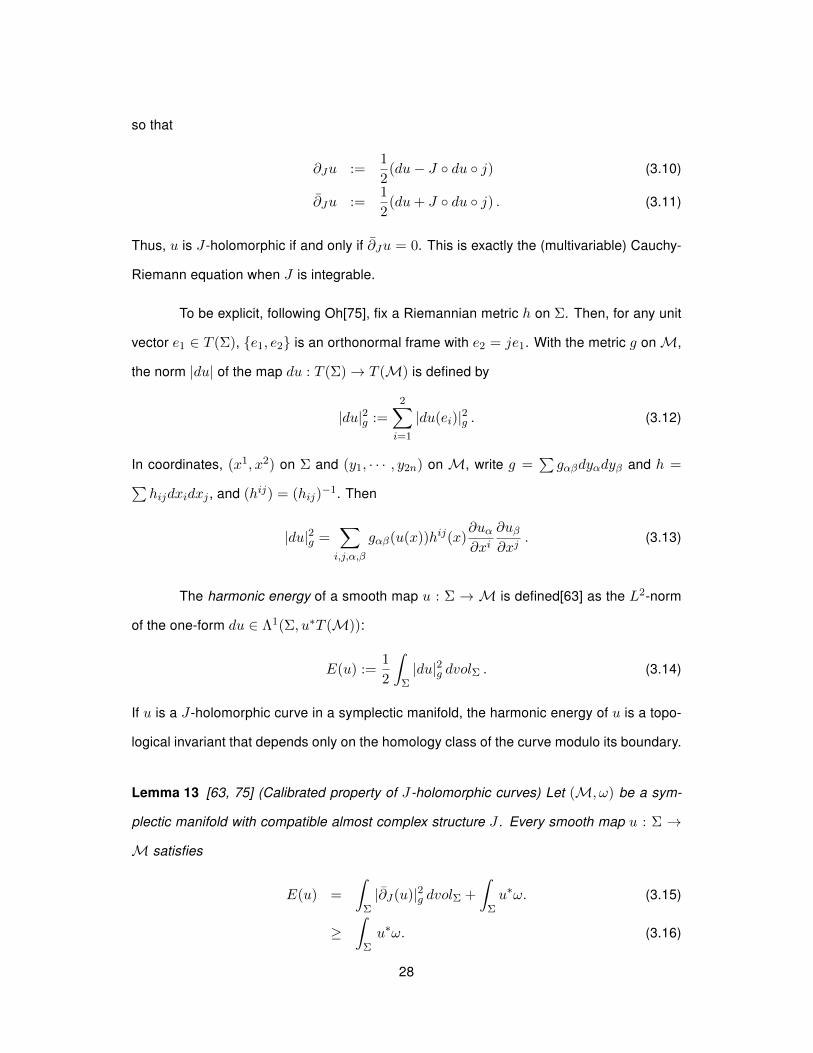
so that

∂Ju :=1

2(du− J du j) (3.10)

∂Ju :=1

2(du+ J du j) . (3.11)

Thus, u is J -holomorphic if and only if ∂Ju = 0. This is exactly the (multivariable) Cauchy-

Riemann equation when J is integrable.

To be explicit, following Oh[75], fix a Riemannian metric h on Σ. Then, for any unit

vector e1 ∈ T (Σ), e1, e2 is an orthonormal frame with e2 = je1. With the metric g onM,

the norm |du| of the map du : T (Σ)→ T (M) is defined by

|du|2g :=2∑i=1

|du(ei)|2g . (3.12)

In coordinates, (x1, x2) on Σ and (y1, · · · , y2n) on M, write g =∑gαβdyαdyβ and h =∑

hijdxidxj , and (hij) = (hij)−1. Then

|du|2g =∑i,j,α,β

gαβ(u(x))hij(x)∂uα∂xi

∂uβ∂xj

. (3.13)

The harmonic energy of a smooth map u : Σ →M is defined[63] as the L2-norm

of the one-form du ∈ Λ1(Σ, u∗T (M)):

E(u) :=1

2

∫Σ|du|2g dvolΣ . (3.14)

If u is a J -holomorphic curve in a symplectic manifold, the harmonic energy of u is a topo-

logical invariant that depends only on the homology class of the curve modulo its boundary.

Lemma 13 [63, 75] (Calibrated property of J -holomorphic curves) Let (M, ω) be a sym-

plectic manifold with compatible almost complex structure J . Every smooth map u : Σ →

M satisfies

E(u) =

∫Σ|∂J(u)|2g dvolΣ +

∫Σu∗ω. (3.15)

≥∫

Σu∗ω. (3.16)

28

and equality holds precisely when u is J -holomorphic. When Σ is a closed surface without

boundary (resp. with boundary fixed or with free boundary on a fixed lagrangian submani-

fold), then∫u∗ω is constant in a fixed homology class (resp. in a relative homology class).

In this case, if u is J -holomorphic map, then the metric area AreagJ (u) := E(u) depends

only on [u], the homology class represented by u:

AreagJ (u) = [ω]([u]) (3.17)

Corollary 14 [75] If u : Σ→M is a J -holomorphic map, then near each regular point of u

on Σ, the image of u is a minimal surface with respect to the metric gJ = ω(·, J ·).

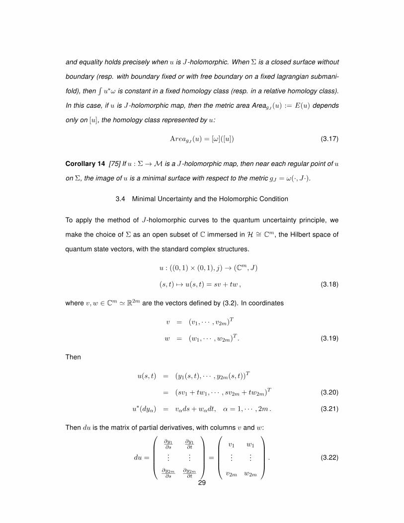
3.4 Minimal Uncertainty and the Holomorphic Condition

To apply the method of J -holomorphic curves to the quantum uncertainty principle, we

make the choice of Σ as an open subset of C immersed in H ∼= Cm, the Hilbert space of

quantum state vectors, with the standard complex structures.

u : ((0, 1)× (0, 1), j)→ (Cm, J)

(s, t) 7→ u(s, t) = sv + tw , (3.18)

where v, w ∈ Cm ' R2m are the vectors defined by (3.2). In coordinates

v = (v1, · · · , v2m)T

w = (w1, · · · , w2m)T . (3.19)

Then

u(s, t) = (y1(s, t), · · · , y2m(s, t))T

= (sv1 + tw1, · · · , sv2m + tw2m)T (3.20)

u∗(dyα) = vαds+ wαdt, α = 1, · · · , 2m. (3.21)

Then du is the matrix of partial derivatives, with columns v and w:

du =

∂y1∂s

∂y1∂t

......

∂y2m∂s

∂y2m∂t

=

v1 w1

......

v2m w2m

. (3.22)

29

Denote by G the flat metric on Cm; Gαβ = δαβ . Pulling back the metric G to get h

on Σ,

h = u∗G = u∗

(∑α

(dyα)2

)=∑α

(u∗(dyα))2

= |v|2ds2 + |w|2dt2 + 2〈v, w〉ds dt . (3.23)

Comparing to h =∑hijdsidtj gives h11 = |v|2, h22 = |w|2, and h12 = h21 = 〈v, w〉.

Inverting (hij) and using (3.13) we have

|du|2 =∑α,i,j

hij(s, t)(∂yα∂s

∂yα∂t

)ij

=1

det(hij)(2|v|2|w|2 − 2〈v, w〉2) = 2 . (3.24)

Hence, evaluating the harmonic energy (3.14), we find that

E(u) =

∫ΣdvolΣ =

∫Σ

√det(hij)ds ∧ dt

=√|v|2|w|2 − 〈v, w〉2 . (3.25)

Thus, looking back at (3.4), we see that E(u) is equal to the area of the parallelogram de-

fined by the vectors (3.2), as well as to the square root of the determinant of the covariance

matrix on the left hand side of the quantum uncertainty principle. We have shown

Lemma 15 The harmonic energy E(u) of the immersion u which maps the open unit

square into the parallelogram defined by the vectors (3.2) is equal to the area of the paral-

lelogram√D(A, B, z).

E(u) =

√(∆A)2

z (∆B)2z − (C(A, B)z)2 . (3.26)

Now let us specify the J -holomorphic condition for the map (3.18). Let

j =

0 −1

1 0

30

and let J be the 2m × 2m block diagonal matrix with each block equal to the 2 × 2 matrix

j. The J -holomorphic condition

∂Ju =1

2

v1 − w2 w1 + v2

v2 + w1 w2 − v1

v3 − w4 w3 + v4

v4 + w3 w4 − v3

......

= 0 (3.27)

is equivalent to the component-wise Cauchy-Riemann equations:

vα =∂yα∂s

=∂yα+1

∂t= wα+1

vα+1 =∂yα+1

∂s= −∂yα

∂t= −wα , (3.28)

Thus, we have the result:

Lemma 16 The map u defined in (3.18) is J -holomorphic if and only if vα + ivα+1 =

−i(wα + iwα+1) if and only if v = −Jw.

Now observe that the off-diagonal part C(A, B)z = g(Az, Bz) of the covariance matrix is

real and hence vanishes in the case that v = −Jw. Therefore, we have the following:

Corollary 17 When the map u defined in (3.18) is J -holomorphic, the covariance matrix

has vanishing off-diagonal components and minimum determinant. In this case, the unit

square is mapped to a square.

Now we can compare the uncertainty principle inequality and the minimal surface

inequality term by term. By the lemma, the left sides of (2.36) and (3.15) are equal, and

the right sides are each equal to the symplectic area of the parallelogram determined by

the vectors (3.2). This makes it possible to compare the additional terms that occur when

equality is not achieved, that is, the antiholomorphic part of the image of the map u on the

one hand, and orthogonal part lost when v is projected onto w on the other hand. It could

be illuminating to exhibit this comparison explicitly. Observe the topological invariant for QT.31

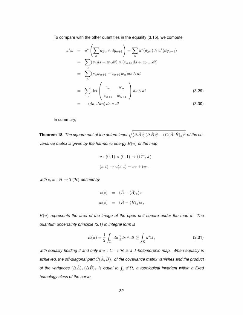
To compare with the other quantities in the equality (3.15), we compute

u∗ω = u∗

(∑α

dyα ∧ dyα+1

)=∑α

u∗(dyα) ∧ u∗(dyα+1)

=∑α

(vαds+ wαdt) ∧ (vα+1ds+ wα+1dt)

=∑α

(vαwα+1 − vα+1wα)ds ∧ dt

=∑α

det

vα wα

vα+1 wα+1

ds ∧ dt (3.29)

= −〈du, Jdu〉 ds ∧ dt (3.30)

In summary,

Theorem 18 The square root of the determinant√

(∆A)2z (∆B)2

z − (C(A, B)z)2 of the co-

variance matrix is given by the harmonic energy E(u) of the map

u : (0, 1)× (0, 1)→ (Cm, J)

(s, t) 7→ u(s, t) = sv + tw ,

with v, w : H → T (H) defined by

v(z) = (A− 〈A〉z)z

w(z) = (B − 〈B〉z)z ,

E(u) represents the area of the image of the open unit square under the map u. The

quantum uncertainty principle (3.1) in integral form is

E(u) =1

2

∫Σ|du|2gds ∧ dt ≥

∫Σu∗Ω , (3.31)

with equality holding if and only if u : Σ → H is a J -holomorphic map. When equality is

achieved, the off-diagonal part C(A, B)z of the covariance matrix vanishes and the product

of the variances (∆A)z (∆B)z is equal to∫

Σ u∗Ω, a topological invariant within a fixed

homology class of the curve.

32

3.5 Examples

By choosing the operators A and B judiciously, we can use the understanding of the un-

certainty principle gained from the holomorphic map approach by specific applications to

quantum systems. An obvious choice is X and P , the position and momentum operators,

since the uncertainty principle is most commonly couched in these terms. Moreover, in

analogy to the cotangent bundle phase space of classical mechanics, we can view (x, p)

as canonical coordinates on the quantum phase space P (H). Recall that taking the hori-

zontal component of Az, that is (A − 〈A〉)z, is equivalent to projection onto P (H). Thus,

by choosing A = X and B = P , the image of the surface Σ under the map u is a two-

dimensional region in P (H) and Ω(Xz, P z) represents its symplectic area. With these

coordinates, Ω = dx ∧ dp, so that Ω(Xz, P z) = Im〈z, [X, P ]z〉 = ~. We may interpret

the result of the theorem to mean that when the map u is J -holomorphic, the harmonic en-

ergy (a metric area) has the value ~. de Gosson and Leuf[34] have analyzed this example

in terms of the symplectic capacitance of the quantum phase space, and pointed out its

meaning in terms of Gromov’s nonsqueezing theorem.

If we allow the operators A and B to be related through time-dependence, as in

B(t) = U(t)BU(t)−1 for a family of unitaries U(t), we can study the linear response of a

quantum system to a perturbation by using a Kubo Formula,[38]

δ〈A〉 = 〈A〉 − 〈A〉0 =i

~

∫dt〈ψ, [B(t), A]ψ〉 (3.32)

We return to this example in Chapter 5, where it is shown that the dielectric response

function in the form (3.32) is equivalent to the curvature of a connection on a principal

bundle.

A closely related quantity derived from a cumulant generating function[88] is the

second cumulant average

〈XiXj〉c = 〈XiXj〉 − 〈Xi〉〈Xj〉 . (3.33)

For a finite system, X :=∑N

i=1 xi, so that X/N is the position operator for the center of33

mass of the N electrons in the finite volume. For an extended many-body system, similar

quantities are defined in [88] by using special "twisted" boundary conditions. These authors

find the second moment (3.33)

〈XiXj〉c =V

2π

3 ∫dkTij(k)

Tij(k) = 〈∂kiΦk, ∂kjΦk〉 − 〈∂kiΦk,Φk〉〈Φk, ∂kjΦk〉, (3.34)

where Φk is a many-body cell-periodic wave function, and Tij(k) is a gauge-invariant quan-

tity called the quantum geometric tensor.[15] Analysis of these results using holomorphic

maps could provide interesting and useful insights.

An important set of examples takes one of the operators in (3.1) to be the Hamil-

tonian energy operator, H . Viewing the quantum system as an integral dynamical system,

the system dynamics follows the flow of the associated vector field, as described in section

2.5. This flow is tangent to the lagrangian submanifolds defined as the intersection of the

level sets of the constants of the motion. If we choose a second vector field to be normal

to a lagrangian submanifold, the associated flow will take the system away from the one

determined by H , producing a variation or deformation of the dynamical flow. The mean

curvature vector field determines such a deforming flow, since it is normal to the immersed

submanifold. The choice of A as the Hamiltonian operator H , and B as a variation or defor-

mation of H is an instance of the energy-time uncertainty principle of quantum mechanics.

By choosing a family of immersion maps ut : Σ→M so that the boundary of the image of

u0 lies in a lagrangian submanifold of P (H) (or ofH), we can study these deformations and

gain information about topological invariants. In the next chapter, we study the mean curva-

ture flow and associated Maslov cohomology class, with particular interest in its relationship

to the geometric phase of an evolving quantum system.

As a specific example, consider the following J -map that could provide insight into

the problem of the intersection of Lagrangian tori, as in a family of integrable systems. We

can specify that the boundary of Σ maps into a torus which is a Lagrangian submanifold of

34

M , as follows.

u : ((0, 2π)× (0, 2π), j)→ (C, J)

(s, t) 7→ u(s, t) = vRs + wRt (3.35)

Rθ =

cos θ − sin θ

sin θ cos θ

with v = (v1, · · · , v2m)T , and w = (w1, · · · , w2m)T defined by (3.2) as before. Then

u(s, t) =

v1 cos s− v2 sin s+ w1 cos t− w2 sin t

v1 sin s+ v2 cos s+ w1 sin t+ w2 cos t

...

. (3.36)

Using the matrices j and J as before to compute ∂Ju = 12(du+J du j), we find that the

condition ∂J u = 0 for u to be J -holomorphic is−v1 sin s− v2 cos s− w1 cos s+ w2 sin s −w1 sin t− w2 cos t+ v1 cos t+ v2 sin t

v1 cos s− v2 sin s− w1 sin s− w2 cos s w1 cos t− w2 sin t− v1 sin t+ v2 cos t

......

= 0 ,

which holds for all s, t ∈ (0, 2π) if and only if v1 = w2, v2 = −w1 if and only if v = −Jw.

This is precisely the result found with the linear map (3.18). In the present context, we would

like to interpret the result as an equivalence between the holomorphic map condition and

the condition for transversality of two lagrangian tori corresponding to initial and deformed

integrable systems.

Pulling back the metric h = u∗g yields (after some algebra) h =∑2

i,j=1 hijdsidtj

with

h11 = |v|2 = g(v, v),

h22 = |w|2 = g(w,w),

h12 = h21 = g(v, w) cos(s− t) + g(v, Jw) sin(s− t) . (3.37)

35

Chapter 4

DEFORMATIONS OF A QUANTUM SYSTEM

Let us now consider deformations of an integrable quantum system. We would like to

compare two Lagrangian submanifolds L and L′ = φT (L) of a symplectic manifold M,

where φtTt=0 is a family of (Hamiltonian) symplectomorphisms parameterized by t. As we

study this question, keep in mind two perspectives:

1) Let u0 : Σ →M be a J -map that maps the boundary of Σ into L and similarly,

let uT : Σ →M map the boundary of Σ into L′. The pullback bundle u∗(TM) is a way to

get the Maslov classes for comparison[72]. Transversality is the key feature.

2) Consider the single map (3.35), where v := Az, w := U(T )AU(T )−1z, and U(t)

is the unitary operator corresponding to φt.

4.1 Symplectic and Hamiltonian Deformations

Let Diff(M) denote the group of diffeomorphisms of a smooth manifold M. An action of

a Lie group G on M is a group homomorphism ψ : G → Diff(M) defined by g 7→ ψg.

Let (M, ω) be a symplectic manifold and let Symp(M, ω) denote the (infinite dimensional)

group of symplectomorphisms ofM, that is, the group of diffeomorphisms ofM that pre-

serve ω: Symp(M, ω) = ψ ∈ Diff(M) |ψ∗ω = ω. The action ψ is a symplectic action

if

ψ : G→ Symp(M, ω) ⊂ Diff(M) .

Let G be a Lie group with action ψ : G→ Diff(M), and g the Lie algebra of G with dual g∗.

Then the action ψ is a hamiltonian action if there exists a map

µ :M→ g∗

that satisfies the following two conditions:

1. For each ξ ∈ g, let µξ : M → R, µξ(p) := 〈µ(p), ξ〉 be the component of µ along

ξ, and let ξ] be the fundamental vector field onM generated by the one-parameter36

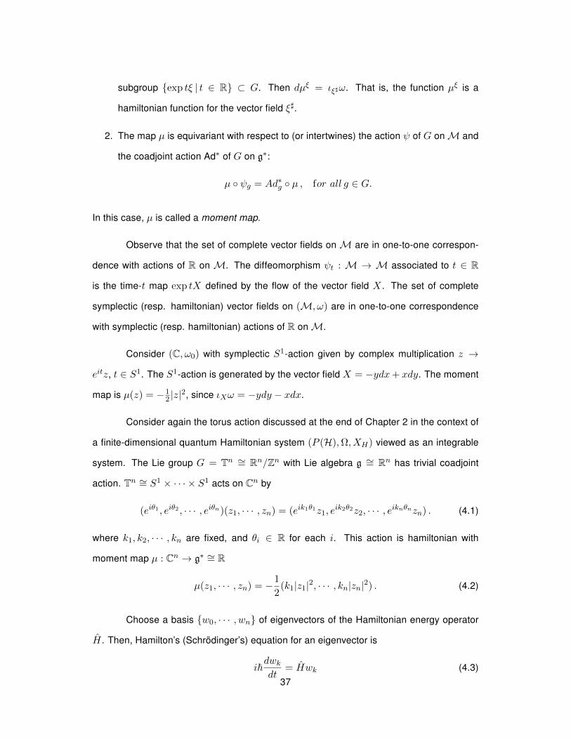
subgroup exp tξ | t ∈ R ⊂ G. Then dµξ = ιξ]ω. That is, the function µξ is a

hamiltonian function for the vector field ξ].

2. The map µ is equivariant with respect to (or intertwines) the action ψ of G onM and

the coadjoint action Ad∗ of G on g∗:

µ ψg = Ad∗g µ , for all g ∈ G.

In this case, µ is called a moment map.

Observe that the set of complete vector fields onM are in one-to-one correspon-

dence with actions of R on M. The diffeomorphism ψt : M → M associated to t ∈ R

is the time-t map exp tX defined by the flow of the vector field X. The set of complete

symplectic (resp. hamiltonian) vector fields on (M, ω) are in one-to-one correspondence

with symplectic (resp. hamiltonian) actions of R onM.

Consider (C, ω0) with symplectic S1-action given by complex multiplication z →

eitz, t ∈ S1. The S1-action is generated by the vector field X = −ydx+ xdy. The moment

map is µ(z) = −12 |z|

2, since ιXω = −ydy − xdx.

Consider again the torus action discussed at the end of Chapter 2 in the context of

a finite-dimensional quantum Hamiltonian system (P (H),Ω, XH) viewed as an integrable

system. The Lie group G = Tn ∼= Rn/Zn with Lie algebra g ∼= Rn has trivial coadjoint

action. Tn ∼= S1 × · · · × S1 acts on Cn by

(eiθ1 , eiθ2 , · · · , eiθn)(z1, · · · , zn) = (eik1θ1z1, eik2θ2z2, · · · , eiknθnzn) . (4.1)

where k1, k2, · · · , kn are fixed, and θi ∈ R for each i. This action is hamiltonian with

moment map µ : Cn → g∗ ∼= R

µ(z1, · · · , zn) = −1

2(k1|z1|2, · · · , kn|zn|2) . (4.2)

Choose a basis w0, · · · , wn of eigenvectors of the Hamiltonian energy operator

H . Then, Hamilton’s (Schrödinger’s) equation for an eigenvector is

i~dwkdt

= Hwk (4.3)

37

wk(t) = ei~λkwk (4.4)

Now consider parameterized families of R actions. A symplectic isotopy of M is

a smooth map [0, 1] ×M → M : (t, q) 7→ ψt(q) such that ψt ∈ Symp(M, ω) for each

t ∈ [0, 1] and ψ0 = id. Any such isotopy is generated by a unique family of vector fields

Xt :M→ T (M) such thatd

dtψt = Xt ψt. (4.5)

Since ψt is a symplectomorphism for every t, the vector fields Xt are symplectic and so,

each associated one-form is closed:

dιXtω = 0.

If all of these one-forms are exact, then there exists a smooth family of Hamiltonian functions

Ht :M→ R such that

ιXtω = dHt . (4.6)

In this case, the family ψt is a hamiltonian isotopy, and the family Ht is a time-dependent

Hamiltonian. If M is simply connected, then every symplectic isotopy is hamiltonian. Oh

studied isotopies of lagrangian submanifolds.[70, 71, 72, 73]

A symplectomorphism ψ ∈ Symp(M, ω) is called hamiltonian if there exists a

hamiltonian isotopy ψt ∈ Symp(M, ω) from ψ0 = id to ψ1 = ψ. The space of hamilto-

nian symplectomorphisms, denoted by Ham(M, ω), is a normal subgroup of Symp(M, ω),

and its Lie algebra is the algebra of all hamiltonian vector fields.[62]

The flux homomorphism[62] Flux : Symp0(M, ω)→ H1(M,R) is defined by

Flux(ψt) =

∫ 1

0[ι(Xt)ω]dt ∈ H1(M;R) (4.7)

where Xt is determined by (4.5).

Now consider the application of the concepts of symplectic and hamiltonian iso-

topies to the quantum dynamics of time-dependent Hamiltonians. Giavarini and Onofri[42]

studied Hamiltonians of the form

H(t) = U(t)H(0)U(t)† , (4.8)38

where U(t) takes values in a unitary irreducible representation of a Lie group, and H(0)

is a generator in its Lie algebra g. Applications include the geometric phase and coherent

states. It would be interesting to study these as examples of hamiltonian isotopies. Consider

the following conjectures for future study:

Conjecture 1: Lagrangian deformations correspond to coadjoint orbits of the symplectic

group.

Conjecture 2: Hamiltonian deformations correspond to coadjoint orbits of the unitary group.

The geometric phase is the holonomy of a curve (class) in the baseM of a principle

U(1) bundle. In the adiabatic case, there is a correspondence between each point in M

and a lagrangian submanifold, so that a path in M corresponds to a family of lagrangian

submanifolds.

4.2 Mean Curvature and the Maslov Class

Let us now consider the time evolution of quantum states, viewed as a Hamiltonian dynam-

ical system. For the initial system, take the example (P (H),Ω0, XH) with Hilbert space

H ∼= Cn+1 from section 2.5, and recall that the toral action of the projection operators Pj

foliates H into lagrangian tori of dimension n + 1, and foliates the phase space P (H) into

lagrangian tori of dimension n. The lagrangian condition means that means, in particular,

that Ω(u, v) = 0 for any u, v ∈ T (L).

There are many possibilities to consider: How does a system relax after an initial

perturbation? How do states of a perturbed system evolve to eigenstates of a future Hamil-

tonian? Will an unperturbed system initially in L evolve into another lagrangian submanifold

L′ of the same leaf and foliation? For now, we will not commit to any of these questions, but

instead ask: How do states initially in L evolve along the flow of the mean curvature vector

field determined by L? A nice property of the case of a lagrangian submanifold embedded

in a symplectic manifold is that the submanifold evolves under the mean curvature flow into

a lagrangian submanifold, so that the system remains integrable.

Furthermore, mean curvature plays an important role in the symplectic topology

39

of Lagrangian submanifolds.[73]. An enlightening discussion of the Maslov class may be

found in [12]. See also the paper by Cieliebak and Goldstein [26], in which they prove

the following relation between the symplectic area, Maslov class, and the mean curvature

one-form of a Lagrangian immersion in a Kähler-Einstein manifold.

λω(F ) = πµ(F ) + σL(∂F ) . (4.9)

Morvan[64] proved that the mean curvature vector Hi of the lagrangian immersion

i : L → Cn represents the Maslov cohomology class of i. More precisely, the one form

1παHi on L defined by

αHi : T (L)→ R,

αHi(v) = Ω(Hi, v)|T (L) (4.10)

represents the Maslov class µ ∈ H1(L,Z).

Next we show a calculation of the mean curvature vector Hi for the Lagrangian

immersion i : L = Tm → Cm.

LetG and Ω be the real and imaginary parts of the standard Hermitian inner product

on Cm. By the definition of a Lagrangian immersion, i∗(Ω) = 0 on all points of L. Putting

the metric i∗(G) on L makes i an isometric immersion. The normal bundle N(Tm) is the

orthogonal complement to T (Tm) in T (Cm).

Choose an orthonormal basis ψ0, ..., ψn for H consisting of eigenvectors of H .

Label the one-dimensional (circle) components of Tm as Sk, k = 1, · · · ,m, where Sk =

zk = xk + iyk : xk, yk ∈ Rx2k + y2

k = |rk|2.

The mean curvature vector Hi of the immersion i at z ∈ L is the normal vector

Hi(z) := Tr II =

m∑k=1

II(vk, vk) , (4.11)

where v1, · · · , vm is an orthonormal basis of Tz(Cm), and II is the second fundamental

40

form associated to i, defined as

II : T (Tm)⊗ T (Tm)→ N(Tm)

II(U, V ) = ∇UV −∇UV = pN (∇UV ) , (4.12)

where ∇ is the trivial metric on Cm, ∇ is the Levi-Civita connection on T (Tm), and pN is

the orthogonal projection onto N(Tm).

At a point z = (z1, · · · , zm) ∈ Tm, in coordinates zk = xk + iyk, the unit vector

tangent to the circle Sk with radius rk is

vk =1

rk

(yk

∂

∂xk− xk

∂

∂yk

). (4.13)

The connection ∇ corresponds to the flat metric on Cm. Then

∇vk(vk) = ∇( ykrk

∂

∂xk−xkrk

∂

∂yk

)(ykrk

∂

∂xk− xkrk

∂

∂yk

)(4.14)

(more here)

∇vk(vk) = − 1

r2k

(xk

∂

∂xk+ yk

∂

∂yk

). (4.15)

This vector is already along the normal direction (along the radial vector xk∂∂xk

+yk∂∂yk

), so

pN∇vk(vk) = − 1

r2k

(xk

∂

∂xk+ yk

∂

∂yk

), (4.16)

so that the mean curvature vector is

Hi = −m∑k=1

1

r2k

(xk

∂

∂xk+ yk

∂

∂yk

). (4.17)

In our coordinates, Ω =∑m

k=1 dxk ∧ dyk, so that the mean curvature one-form is

αHi :=1

πiHiΩ =

m∑k=1

1

πr2k

(ykdxk − xkdyk) . (4.18)

A theorem of Dazord[31] states that, on Kähler manifolds, the one-form αHi satisfies

dαHi = i∗ρ , (4.19)

where i : L → (M,Ω) and ρ is the Ricci form of the Kähler metric G. In, particular, if

(M,Ω, J) is Einstein-Kähler, that is, if ρ = cΩ for c ∈ R, then the one-form αHi on L is

closed and so defines a real cohomology class on L.41

Here we calculate the Maslov class for a typical generator of the homology basis

γk. For (xk, yk) = (rk cos(2πt), rk sin(2πt)), t ∈ [0, 1], define

γk(t) = (0, 0, · · · , rk cos(2πt), rk sin(2πt), 0, · · · ) . (4.20)

Then ∫γk

αHi =1

π

∫ 1

0

−2π

r2k

(r2k sin2(2πt) + r2

k cos2(2πt))dt = −2 . (4.21)

The Maslov class takes each of the generators to the number 2.

Taking the exterior derivative of the result (4.18) for the one-form αHi corresponding

to the immersion i : L = TN → CN gives

dαHi =m∑k=1

1

πr2k

dxk ∧ dyk . (4.22)

In summary, we have calculated the mean curvature vector fieldHi of an immersion

i : L →M of a lagrangian submanifold L inM; Hi is the trace of the second fundamental

form of L. As such, it is a section of the normal bundle to L inM, and generates a local flow

on L. A family of submanifolds evolves under mean curvature flow if the velocity at each

point of a submanifold is given by the mean curvature vector at that point. In addition, the

mean curvature one-form αHi := 1π ιHiΩ represents the Maslov class µ ∈ H1(L,Z).[64]

Since the quantum phase space P (H) is Einstein-Kähler, the one form αHi on L = Tn ⊂

P (H) is closed[31], and so defines a real cohomology class in H1(L,R). In particular,

this means that lagrangian submanifolds stay lagrangian under the mean curvature flow on

P (H). Moreover, in this case, under a Hamiltonian isotopy of the Lagrangian immersion

i : L →M, the one forms αHt represent the same cohomology class.

4.3 Berry’s Phase and Mean Curvature Flow

The original descriptions of the quantum geometric phase by Berry[14] and Simon[87] were

not in terms of the principal bundle U(1) → S(H)π−→ P (H) used to describe the geometric

phase in Chapter 2. Instead, Berry[14] considered a quantum system that can be described

in terms of a parameterized family of Hamiltonian operators H(r); the time evolution is

determined by smoothly varying the parameter. In this spirit, let the parameter space be an42

oriented, smooth, compact manifold, denoted byM. Suppose that, for each r ∈ M, H(r)

acts on elements of a complex Hilbert spaceH with inner product 〈, 〉. Berry assumed that,

for each r ∈M, H(r) has a purely discrete spectrum, and that the nth eigenvalue of H(r)

is nondegenerate (has multiplicity one). On a local chart domain V ⊂ M, define a map

sn : V → H so that, for each r ∈ V , sn(r) is an element of the nth eigenspace of H(r)

with 〈sn(r), sn(r)〉 = 1. The eigenvectors sn(r) of H(r) satisfy

H(r)sn(r) = En(r)sn(r) (4.23)

with energies En(r).

Let H(r)r∈M be a family of Hamiltonian operators parameterized by elements of

M and let C : [0, T ] → M, t 7→ r(t) be a path in M. Suppose that a quantum system

is prepared with state vector ψ0 = sn(r(0)). The state vector ψ(t) of the system evolves

according to Schrödinger’s equation

i~ψ′(t) = H(r(t))ψ(t) . (4.24)

If H is slowly altered by varying r, it follows from the quantum adiabatic theorem[53, 67, 11],

that the system will evolve with H and will remain in the nth eigenspace of H(r(t)) for all

t ∈ [0, T ]. Thus, the state vector ψ(t) equals sn(r(t)) modulo a phase factor and may be

written as

ψ(t) = exp(iχn(t)) exp(iβn(t))sn(r(t)) , (4.25)

where χn(t) = −1~∫ t

0 En(r(t′))dt′ is the dynamical phase. The phase function βn(t) is

determined by requiring that ψ(t) satisfy Schrödinger’s equation. Applying (4.24) to (4.25)

and using (4.23) yields

β′n(t)sn(r(t)) = i(sn r)′(t) = ir′(t)(sn(r(t))) = ids(r′(t)) (4.26)

β′n(t) = i〈sn(r(t)), ds(r′(t))〉 . (4.27)

Here, ds(r′(t)) is the derivative of s in the direction r′(t), as in (6.30). Now suppose that

the path C is closed, that is, r(0) = r(T ). In this case, ψ(T ) may differ from ψ(0) only by a

phase factor. The total phase factor change of ψ after traversing C is given by

ψ(T ) = ψ(0) exp(iχn(T )) exp(iβn(C)) , (4.28)43

where the geometrical phase change, known as Berry’s phase,

βn(C) = i

∮〈sn(r(t)), ds(r′(t))〉dt , (4.29)

depends on the geometry ofM and on the path C.

Note the similarity between the expressions (4.29) for Berry’s phase and (2.53)

or (2.52) for the AA phase. In fact, Aharonov and Anandan[3] showed that the AA phase

reduces to Berry’s phase in the adiabatic limit. Simon[87] observed that Berry’s phase could

be interpreted geometrically in terms of a holonomy of a connection in a complex line bundle

over the parameter space M. Wilczek and Zee[94] found a nonabelian generalization of

Berry’s phase for the case of a parameterized family of Hamiltonian operators, each with a

spectrum containing an eigenvalue of fixed multiplicity greater than one.

A goal for future work is to establish the relationship between Berry’s phase and the

mean curvature flow of a quantum system discussed in the prvious section. An outline of

the plan follows. Consider a time-dependent family of immersions,

f : L × [0, 1]→ H∂

∂tf(z, t) = H(z, t) z ∈ H, t ≥ 0 (4.30)

f(·, 0) = f0 , (4.31)

where H(z, t) is the mean curvature vector at z ∈ H, t ≥ 0. Since H(z, t) is an element

of the normal bundle N(L), the mean curvature flow is normal to the level surfaces of the

integrable system. We want to compare the initial and time-evolved states of the system.

A vector ψ ∈ H evolves according to ψt =∑n

k=0 λkPk(t), while the elements of

the phase space P (H) may be written as p(z, t). The following lemma makes it possible to

relate a flow direction (tangent vector) inH to the evolution of a point p(z, t) = |v(t)〉〈v(t)| ∈

P (H).

Lemma 19 [89] Let v, w ∈ H, |v|2 = 1, w := w1 + w2, with w1 ∈ [v], w2 ∈ v⊥. Set

44

v(t) := v + tw. Then

ddt

(〈v(t)|v(t)〉−1 |v(t)〉〈v(t)|

)|t=0 (4.32)

= |w2〉〈v|+ |v〉〈w2| . (4.33)

To compare the flows of a projector P and its variation ˆP , use the lemma to calculate

[ ˆP, P ] = [(|w2〉〈v|+ |v〉〈w2|), |v〉〈v|] = |w2〉〈v| − |v〉〈w2| , (4.34)

similar to multiplication by J . Moreover, Hex := [ ˆP, P ] plays the role of a perturbing Hamil-

tonian operator, since

[Hex, P ] = ˆP . (4.35)

The plan is to relate Hex to the deformation of a quantum integrable system, using the

geometric phase as a watermark.

In his paper[93], Weinstein considered the cyclic evolution of a lagrangian subman-

ifold of a symplectic manifold (M, ω), and presented a way to define a connection over a

foliation on the space Λ(M) of closed, embedded lagrangian submanifolds ofM. In order

to compare to the case of adiabatic motion studied by Berry[14], the evolution is restricted

to isodrastic deformations, which requires the (reduced) action integral

A =

∫Sω

to be constant. Denote by Γω the period group of the symplectic form ω onM , that is, the

subset of R consisting of the integrals of ω over all integer 2-cycles inM. If Γω is trivial or

cyclic, so that Gω := R/Γω is R or a circle, then there is a principal Gω bundle π : Q →M

with a connection form α whose curvature form is the symplectic structure, ω.[93] By Stokes

theorem, the action integral may be written as

A =

∫γα (4.36)

where γ is a loop in M enclosing the surface S. The action integral is thus equal to the

holonomy of the connection α around γ. The holonomy around a loop is unchanged when

the loop undergoes an isodrastic deformation.45

Isodrastic deformations are also called exact deformations, or hamiltonian defor-

mations, since they can be obtained by flowing along globally hamiltonian vector fields. In

particular, they are realized by the trajectories of adiabatically varying completely integrable

systems.

4.4 The Vector Bundle Classification Theorem

The applications to physics that we wish to describe rely heavily on the geometrical struc-

ture of a complex line bundle over a parameter space and the generalization to higher

dimensional spectral bundles, which are not principal bundles, but rather vector bundles.

Hence, this section begins by defining the relevant fiber bundles and the relationships be-

tween them. It is shown that the quantum adiabatic theorem can be viewed as a statement

relating isomorphisms of certain vector bundles to the adiabatic time evolution of a quantum

system.

Here we begin from more general definitions.[51] A bundle is a triple (E, π,B)

where π : E → B is a map. The space B is called the base space, the space E is called

the total space, and the map π is called the projection of the bundle. For each b ∈ B, the

space π−1(b) is called the fiber of the bundle over b.

A bundle map (or bundle morphism) between a pair of bundles (E, π,B) and

(E′, π′, B′) is a pair of maps (h, f) where h : E → E′ and f : B → B′ such that

π′ h = f π. Note that the last equality implies that, for all b ∈ B, h(π−1(b)) ⊂ π′−1(f(b)),

that is, the pair of maps (h, f) maps fibers into fibers. When π is surjective, the map f is

uniquely determined by the map h. If (E, π,B) and (E′, π′, B) are two bundles over B, a

bundle morphism over B (or B-morphism) u : (E, π,B)→ (E′, π′, B) is a map u : E → E′

such that π = π′ u.

If λ = (E, π,B) is a bundle and f is a map from another manifold B′ into the base

B, then the induced bundle or pull-back of λ is the bundle f∗(λ) over B′ with total space

E′ := (b′, p) ∈ B′×E | f(b′) = π(p) and with the projection map π′ : E′ → B′ defined by

π′(b′, p) = b′. There is a natural bundle map from the pull-back bundle f∗(λ) to the original

46

bundle λ, defined as the pair of maps (fλ, f), where fλ : E′ → E and fλ(b′, p) := p.

An n-dimensional complex vector bundle F → Eπ−→ B is a bundle together with the

structure of an n-dimensional complex vector space on each fiber π−1(b) ∼= F such that the

following local triviality condition is satisfied. For each b ∈ B, there exists a neighborhood

U ⊂ B of b and a U -isomorphism h : U × Cn → π−1(U) such that, for all y ∈ U , the

restriction y × Cn → π−1(y) is a vector space isomorphism.

Definition: Canonical vector bundle. The complex Grassmann manifold (or Grass-

mannian), GnN (C), is the set of n-dimensional complex subspaces in CN , provided with

the structure of a complex manifold.[57], p.133. In particular, the Grassmannian G1N (C) is

N -dimensional complex projective space CPN defined in Example 9 of the appendix and

used to describe physical states in quantum mechanics. There is a canonical vector bundle

En over GnN : any point x ∈ GnN is an n-dimensional subspace in CN , and the fiber Fnx over

x is this subspace itself. That is,

En = (v, w) | v ∈ w ⊂ CN ×GnN

π = En → GnN , π(v, w) := w . (4.37)

Example: Spectral line bundle. Let H be a separable Hilbert space. Suppose that

H(x)x∈M is a family of self-adjoint operators on H, and that the family is parameterized

by points x of a smooth manifoldM. Assume that for each x ∈M, H(x) has a multiplicity

one eigenvalue λ(x) that is separated from the rest of the spectrum by a gap, that is, there

exist two real-valued functions f and g on M such that dist[(g(x), h(x);λ(x)] > 0. Also

assume that the function λ : M → R is differentiable. Define a map P : M → CPN

such that Ran P (x) ∼= Vx where Vx is the one-dimensional eigenspace associated to λ(x).

The spectral line bundle F → Eπ−→ M is the one-dimensional vector bundle, with fibers

Fx = π−1(x) ∼= Vx and total space F =⊔x∈M = (x, v) | v ∈ Vx, isomorphic to the

pullback bundle P ∗(E1) of the canonical line bundle over CPN . The generalization to n-

dimensional vector spectral bundles, given in the next section, enables us to study systems

with Hamiltonians with more varied spectra.

47

Next we wish to discuss an important result that we will use to relate the theory of

vector bundles to the adiabatic theorem. That is, any n-dimensional complex vector bun-

dle is isomorphic to a pullback bundle of the canonical vector bundle over the Grassman-

nian GnN (C)[37]. Moreover, the n-dimensional vector bundles are sorted into isomorphism

classes by the homotopy classes of maps into GnN (C). In order to explain this construction,

we first recall some facts about projection operators.

Let N be a closed subspace of a Hilbert space H. The orthogonal complement of

N in H, denoted N⊥, is the set of vectors in H that are orthogonal to N , that is, N⊥ =

x ∈ H | (x, n) = 0 for all n ∈ N. The projection theorem states that every x ∈ H

can be written uniquely as x = z + w, where z ∈ N and w ∈ N⊥. Let P be a bounded

linear operator from H to H. If P 2 = P , then P is called a projector. If P = P ∗, then P

is called an orthogonal projector. The range of a projector P , denoted Ran P , is always

a closed subspace on which P acts as the identity. If P is orthogonal, then P acts as the

zero operator on (Ran P )⊥. In this case, for any x ∈ H, the projection theorem guarantees

the decomposition x = y + z, with y ∈ Ran P and z ∈ (Ran P )⊥. Then Px = y and P is

called the orthogonal projector onto Ran P . Thus, the projection theorem sets up a one to

one correspondence between orthogonal projectors and closed subspaces.[79]

Since the Grassmannian GnN (C) is the manifold of n-dimensional complex sub-

spaces in CN , the projection theorem provides a correspondence between the points of

GnN (C) and orthogonal projectors, as follows. Suppose that u1, · · · , un is a basis for

the closed subspace U ⊂ CN . In the case that N is a finite number, let M∗(N,n;C) be

the space of N × n complex matrices of rank n. Each element of M∗(N,n;C) may be

considered as a set of linearly independent vectors in CN , which, in turn, determines an n-

dimensional complex subspace in CN . Thus, we have the natural projectionM∗(N,n;C)→

GnN (C).[57] If A is the matrix with the vectors u1, · · · , un as columns, then the projection

is the n×N matrix PA = A(A†A)−1A†. Since the matrix P can be bordered by zeros, the

dimension N can be made arbitrarily large.

Two useful identities hold for any differentiable projector function P : [0, 1]→ L(H),

48

t 7→ P (t). By differentiating both sides of the statement P 2 = P , we have

P = PP + PP . (4.38)

Multiplying both sides of (4.38) by P on the right and using P 2 = P again gives

PPP = 0 . (4.39)

Now we can show that an n-dimensional vector bundle over a manifoldM is isomor-

phic to a pullback bundle by an orthogonal projector valued function onM.[37]. Let P (x) be

such a function onM, its values being N ×N matrices and suppose that rank(P (x)) = n,

for all x ∈ M. Then Ran P (x) ∈ GnN , P 2(x) = P (x), and tr P (x) = n. The function P (x)

defines a vector bundle, E , overM as follows. The bundle E overM induced by the map

f = RanP : M→ GnN . (4.40)

is defined as the pull-back of the canonical bundle En by the map f . The fiber Fx of the

bundle E overM is isomorphic to the range of P (x), a subspace in CN .

The GrassmanniansGnN are called classifying spaces for n-dimensional vector bun-

dles. The map (4.40) is called a characteristic map, or classifying map, and is used to state

and prove the classifying theorem of vector bundles. Recall that a homotopy is a continu-

ous one-parameter family of maps: ft : X → Y , t ∈ [0, 1] such that the associated map

F : X × I → Y given by F (x, t) = ft(x) is continuous. Two maps f and g : X → Y are

homotopic provided there is a homotopy ft with f = f0 and g = f1.

Theorem 20 [37, 51] (Classifying Theorem) Any n-dimensional vector bundle over a com-

pact base is isomorphic to a bundle, induced by (4.40) for N sufficiently large. Two such

bundles are isomorphic if and only if their characteristic maps are homotopic for a suffi-

ciently large N .

Fedosov[37] uses the following lemma to prove one implication of the second statement of

the classifying theorem, that is, that n-dimensional vector bundles with homotopic charac-

teristic maps are isomorphic.49

Lemma 21 [37] (Intertwining Lemma) Let P (x, t) be a smooth projector-valued function on

M× [0, 1]. Then there exists an invertible matrix function U(x, t) such that

P (x, t) = U(x, t)P (x, 0)U−1(x, t) . (4.41)

Proof: We fix x = x0 ∈ M and suppress the x-dependence of P and U . Define U(t) as

the solution of

UU−1 = [P , P ] (4.42)

with the initial condition U(0) = 1. (The solution exists since [P , P ] is bounded (Theorem

X.69 [80]).) Define P (t) = U(t)P (0)U−1(t). Then P (t) and the given function P (t) satisfy

the same differential equation

P (t) = [UU−1, P ] . (4.43)

Indeed, from (4.42), we have

[UU−1, P ] = [[P , P ], P ] = PP − PPP − PPP + PP = P (4.44)

by using (4.38) and (4.39). On the other hand,

[UU−1, P ] = UP (0)U−1 + UP (0)dU−1

dt= ˙P . (4.45)

Moreover, since U(0) = 1, P and P have the same initial value. Hence, P and P coincide

everywhere. Thus, we have shown that P (x0, t) = P (x0, t) for all t. The argument holds

for each x ∈M. We need to use joint smoothness in x and t here. ut

Given a homotopy Pt ≡ P (·, t) between the characteristic maps P0 and P1 of two vector

bundles over M, the result (4.41) means that the subspaces Ran P0 and Ran P1 are

isomorphic (and that they are isomorphic to all intermediate subspaces Ran Pt for all t ∈

[0, 1]). Hence the pullback bundles P ∗0 (En) and P ∗1 (En) are isomorphic to each other (and

to all of the intervening pullback bundles P ∗t (En) for t ∈ [0, 1]).

4.5 The Adiabatic Theorem

At first sight, it is perhaps remarkable that a version of the Intertwining Lemma is also

used in proofs[53, 67, 11] of the adiabatic theorem for quantum mechanics. The adiabatic50

theorem is a statement about the validity of an approximation to the dynamics generated by

Hamiltonians that vary slowly in time. Observe that, in general, the Schrödinger equation,

i~ψ = H(t)ψ, with time-dependent Hamiltonian operator H has no stationary states. The

theorem states that, if H(t) varies with t slowly enough, then a system initially in one part

of the spectrum of H(0) will pass through the corresponding part of the spectrum of H(t)

for all t.

To be more precise, let s = t/T , where T is the intrinsic time scale of the system.

In rescaled variables, the Schrödinger equation is

i~dψ(s)

ds= TH(s)ψ(s) , (4.46)

where s ∈ [0, 1]. Under general conditions on H ,[80, Thm. X.71] there exists a unitary

propagator UT on L2(Rn) which satisfies

i~∂UT (s; s′)

∂s= TH(s)UT (s; s′) , s ≥ s′ , UT (s′, s′) = 1 . (4.47)

so that ψ(s) = UT (s; s′)ψ(s′) satisfies (4.46). The adiabatic limit corresponds to the limit

T → ∞. Kato’s version[53] of the theorem assumes H(0) has an isolated eigenvalue,

whose multiplicity may be greater than one. Avron, Seiler, and Yaffe[11] and Nenciu[67]

give proofs under less restrictive assumptions about the spectrum of H , that is, H is only

required to satisfy the gap condition: a part of the spectrum of H is separated by an energy

gap from the other parts. Avron and Elgart[4] have proved a version of the theorem with-

out assuming the gap condition. All three proofs[53, 67, 11] of the theorem with the gap

assumption consist of two parts. In the first part, the lemma is used to obtain the unitary

evolution operator Ua representing an adiabatic transformation of the system. In the second

part, one shows that the true dynamic evolution operator determined by equation (4.47) ap-

proaches Ua as T → ∞. It is only for the second part that different proofs are required for

the different assumptions made about the spectra of the Hamiltonians H(t) in [53, 67, 11].

The adiabatic theorem can be understood in terms of a spectral vector bundle over

parameter space, which is a generalization of the spectral line bundle.

Example: Spectral vector bundle. As for the spectral line bundle, suppose that H(x)x∈M51

is a family of self-adjoint operators on a separable Hilbert space H, and that the family

is parameterized by points x of a smooth manifold M. For each x ∈ M, the spectral

theorem for self-adjoint operators associates with H(x) a set of projections that completely

determines H(x). Let P (x) be a map from M to rank n projectors onto a part of the

spectrum of H(x) that is separated from the rest by a gap. Let H → H×M→M be the

trivial bundle over M. Construct a sub-bundle whose fibers Fx are the vector subspaces

Vx = Ran P (x), that is, the fiber at x is Fx := Ran P (x) ⊂ H. We call the vector bundle

F → HP →M with total space HP :=⋃x∈M Fx a spectral bundle. Note that the spectral

bundle F → HP →M is isomorphic to the pullback bundle P ∗(En) and that

HP = (x, p) ∈M× En | RanP (x) = π(p) (4.48)

π = En → GnN , π(v, w) := w .

Now consider how the intertwining lemma serves to establish the existence of a

unitary propagator that determines adiabatic time-evolution of state vectors in HP . A path

[0, 1]→M in the space of parametersM gives rise to a path in the family of parameterized

Hamiltonians, that is, to a time-dependent Hamiltonian H(t) = H(x(t)). In turn, for each

t ∈ [0, 1], P (t) is defined as a projector onto one part of the spectrum σ(H(t)), separated

from the rest of the spectrum by a gap. If we begin the time evolution with a state vector

ψ(0) ∈ Ran P (0) ⊂ H, then P (0)ψ(0) = ψ(0). In the adiabatic approximation, at any later

time t of order T , the state vector ψ(t) is required to be an element of Ran P (t), that is,

P (t)ψ(t) = ψ(t). This requirement is satisfied if there exists a unitary operator Ua that time

evolves ψ:

ψ(t) = Ua(t)ψ(0) (4.49)

where Ua has the intertwining property

P (t) = Ua(t)P (0)U−1a (t) (4.50)

which is (4.41) of the lemma statement. Indeed, if (4.50) holds, then

P (t)Ua(t)ψ(0) = Ua(t)P (0)ψ(0)

= Ua(t)ψ(0) . (4.51)52

Then, by (4.49),

P (t)ψ(t) = ψ(t) . (4.52)

Observe that adiabatic time evolution can be viewed as parallel transport by lifting

a path inM to a path in a Hilbert bundle. If x ∈M is fixed, then Hx := H(x), regarded as

time-independent Hamiltonian, generates a one-parameter group Ux(t) := exp(−itHx) |

t ∈ R. Take a sequence of partitions of a given interval [s, t]

s ≡ t0 < t1 < · · · tn−1 < tn ≡ t, lim supn→∞

(tk−1 − tk) = 0 , (4.53)

we can represent a unitary propagator as a limit

U(t, s)ψ = limn→∞

Ux(tn)(tn − tn−1)Ux(tn−1)(tn−1 − tn−2) · · ·Ux(t1)(t1 − t0)ψ (4.54)

see [2, p.59]

From the proof of the lemma, it is clear that Ua satisfies (4.50) if Ua satisfies

i~dUa(s)

ds= THK(s)Ua(s) (4.55)

HK(s) :=i~T

[P , P ] . (4.56)

The solution Ua determined from (4.55) with the “Kato Hamiltonian” (4.56) is not unique.

Avron et al.[11] showed that the requirement that the adiabatic evolution approximates the

true physical evolution “as best as possible” determines it uniquely. This is the evolution

generated by

Ha(s, P ) := H(s) + i/τ [P ′(s), P (s)] . (4.57)

The crux of the adiabatic theorem is that the true time evolution operator UT , which solves

(4.47), is approximated by Ua in the adiabatic limit:

Theorem 22 [53, 67, 11](Adiabatic theorem) Let H(s) be a smooth family of Hamiltoni-

ans, s = t/T ∈ [0, 1], and let UT (s) be the true time evolution operator (4.47). Let P (s)

be the family of finite rank projectors onto a band of the spectrum σ(H(s)) separated by a

gap. Then

limT→∞

‖UT (s)P (0)− P (s)UT (s)‖ = 0 .

53

The line bundle over a parameter space,M, described by Simon[87] is a spectral

bundle that is constructed as follows. As in the discussion of Berry’s work, assume H(x)

is a Hermitian operator depending smoothly on the parameters x ∈ M, with an isolated

nondegenerate eigenvalue En(x) depending continuously on x. Then (x, ψ) | H(x)ψ =

En(x)ψ defines a spectral line bundle over parameter space. The fiber at x ∈ M is

the one-dimensional eigenspace Lx of H(x) corresponding to the eigenvalue En(x) and

associated eigenvector ψn(x): Lx = ψ ∈ S(H) | ψ = cψn(x), c ∈ C.

The spectral line bundle over parameter space can be related to the principal bundle

S(H) over P (H) as follows[21]. The principal bundle η : U(1) → S(H)π−→ P (H) used

to describe the Aharonov and Anandan phase is the universal classifying bundle for U(1)

principle fiber bundles and the classifying theorem states that any U(1) principle bundle

overM is isomorphic to the pull-back bundle f∗(η) for some continuous function f :M→

CP∞. The spectral line bundle is the associated bundle of this U(1) principal bundle.

In gauge field theory[18, 32, 65], there is a background field, such as the electro-

magnetic field, that is given by a connectionA defined on a principal bundle over spacetime,

M. The structure group of this bundle represents the internal symmetries of the background

field. The possible interactions of the background field with matter are determined by the

representations of the group. Each particle field ψ is a section of the vector bundle over

M associated to the principle bundle through a group representation. The Hilbert space H

in quantum mechanics is the space of sections of this vector bundle. For example, if the

structure group is U(1), then such a section is a function ψ :M→ C.

Simon[87] observed that the adiabatic theorem defines a connection on such a

vector bundle, which is the same as the Hermitian connection inherited from the embedding

of the total space of this bundle into the Hilbert space. The adiabatic evolution transports

state vectors from the range of the projector P (x) to the range of P (x′). The adiabatic

connection can be taken to be the operator-valued one-form[10]

A(P )(x) = −[(dP )(x), P (x)] , (4.58)

54

and the covariant derivative corresponding to the adiabatic connection is

∇ := d+A = Pd . (4.59)

In summary, we have given an interpretation of the adiabatic theorem in terms of

the intertwining lemma used to prove the vector bundle classifying theorem. To link the

discussion with Weinstein’s[93] interpretation of the adiabatic theorem in terms of cyclic

evolution of a lagrangian submanifold of a symplectic manifold, the lemma can be used

to define an isomorphism of lagrangian subbundles defined on the lagrangian tori corre-

sponding to an evolving integrable Hamiltonian system. For each lagrangian immersion

i : L → P (H) along a path in Λ(L), define a line bundle over L, determined by a one

dimensional eigenspace of the Hamiltonian operator H(t), and corresponding projection

operator, P (z, t), z ∈ L. The time evolution problem may be viewed as a homotopy of

classifying maps

P (z, t) = U(z, t)P (z, 0)U(z, t)−1 (4.60)

dU

dtU−1 =

[dP

dt, P

](4.61)

By the classifying theorem of vector bundles, the homotopy P (z, t) gives an isomorphism

of the line bundles. This is a plan for future work.

55

Chapter 5

ADIABATIC CURVATURE AND THE RESPONSE OF A CRYSTALLINE SOLID

This chapter discusses the curvature of the connection on a fiber bundle associated with

the energy spectrum of a periodic Schrödinger operator, and shows the relationship be-

tween this curvature and an electromagnetic linear response function. The curvature of the

connection of the spectral bundle is the pullback of the symplectic form on P (H). The first

Brillouin zone is a parameter space and a moduli space of connections on the space of

lattice periodic wave functions.

5.1 Symplectic Structure of the Periodic Solid

Let a1, · · · , aN ∈ RN be N linearly independent vectors. The set

Λ = a ∈ RN | a =N∑i=1

miai, mi ∈ Z (5.1)

is called the lattice generated by aiNi=1.

The set Λ is a normal subgroup of RN , viewed as a group under addition. The set

of equivalence classes under the equivalence relation x ∼ y if and only if x− y ∈ Λ is itself

a group, denoted by Rn/Λ. That is, the equivalence class of x ∈ RN is [x] = y ∈ RN |x ∼

y and RN/Λ = [x] |x ∈ RN. In addition to being a group, RN/Λ is a smooth manifold,

which is an N -dimensional torus, TN . Indeed, let Q denote the half open parallelepiped

spanned by the ai, that is,

Q := y ∈ RN | y = x1a1 + · · ·xNaN , 0 ≤ xi < 1 ∀i . (5.2)

The map Q → RN/Λ, x 7→ [x] is injective; its inverse is a coordinate map for RN/Λ. The

translates of Q cover RN in a space-filling, one-to-one manner:⋃a∈Λ aQ = RN . Hence,

Q is called a primitive cell of the lattice.

In this chapter, we are interested in functions that are periodic with respect to Λ. A

function f : RN → R is periodic with period a, if f(x + a) = f(x) whenever a ∈ Λ. For

example, the function f(x) = eig·x has period a if and only if eig·(x+a) = eig·a. This is true56

if and only if eig·a = 1, that is, if and only if g · a = 2πn, for some n ∈ Z. Thus, we are

interested in the set g ∈ RN | g · a ∈ 2πZ for all a ∈ Λ.

Let Λ be a lattice in RN . Define the dual basis gjN1 by aigj = 2πδij . The dual

lattice Λ∗ = g ∈ RN | g =∑N

j=1mjgj , mj ∈ Z is called the reciprocal lattice and

B := y ∈ RN | y = x1g1 + · · ·xNgN , 0 ≤ xi < 1 ∀i ∼= RN/Λ∗ (5.3)

is called the Brillouin zone.

Let us restrict our attention to the caseN = 3. We will show that the manifoldQ×B

is a symplectic manifold. Let a1, a2, a3 be a basis of primitive translation vectors of the

lattice, Λ. The volume of the 3d parallelepiped spanned by a1, a2, a3 may be written in

terms of the triple scalar product,

Vcell = a1 · (a2 × a3) (5.4)

The standard definition of the dual basis is

b1 =2π

Vcell(a2 × a3) , b2 =

2π

Vcell(a3 × a1) , b3 =

2π

Vcell(a1 × a2) . (5.5)

Viewing the triple scalar product as a volume form on the unit cell,

vol : TQ × TQ × TQ → R

vol(x1, x2, x3) = x1 · (x2 × x3) = Vcell (5.6)

Then the dual vector b1 is a map TQ → R,

b1(·) =2π

Vcellvol(·, a2, a3) (5.7)

that is, b1 is a one-form on Q, and similarly, so are b2 and b3. Define a two-form on Q× B

by

ω((s1, n1), (s2, n2)) = n2(s1)− n1(s2) . (5.8)

Compare to the canonical symplectic form on the cotangent bundle of a torus: ω =∑3

i=1 dri∧

dki. Here, b1 = kidri.

57

5.2 The Spectral Bundle and the One-Band Subbundle

Consider a single electron in RN subject to a periodic potential, V . The Hamiltonian for the

electron in the lattice is

H =p2

2m+ V , (5.9)

where p = −i~∇x. We assume here that V satisfies∫Q |V (x)|2dnx < ∞. The translation

operators Tj = exp(iaj · p/~), defined by their operation on wave functions ψ ∈ L2(RN ):

Tjψ(x) = ψ(x + aj), then commute with the Hamiltonian and with each other. Hence, H

has eigenfunctions which are simultaneously eigenfunctions of the translation operators.

The eigenvalues of Tj may be parameterized as λj = exp(ik ·aj) by the Bloch wave vector

k, which is an element of the reciprocal lattice. The Bloch wave functions ψ(x + aj) =

exp(ik · aj)ψ(x) are invariant if k is translated by a reciprocal lattice vector. Thus, it is

sufficient to restrict k to the first Brillouin zone.

Now consider the eigenvalue problem

Hψ = Eψ , (5.10)

for H given by (5.9). Since the Hamiltonian commutes with translations by lattice vectors,

we may choose the eigenvectors (weak eigensolutions) of H to be Bloch vectors ψnk with

eigenvalues Enk :

Hψnk = Enkψnk (5.11)

ψnk (x) = eikxunk(x) (5.12)

Here n labels a discrete set of finite-dimensional eigenspaces, and k is a continuous pa-

rameter. The unk are smooth functions with the same periodicity as the lattice. To see why

the result (5.11) with (5.12) is true, substitute (5.12) into (5.10) and find that, for any real

vector k, unk solves

Hkunk = Eku

nk (5.13)

where Hk = e−ikxHeikx.

58

For the Hamiltonian (5.9),

Hk =1

2m(p+ ~k)2 + V . (5.14)

Now solve the eigenvalue equation (5.13), imposing periodic boundary conditions on unk .

As discussed by Odeh and Keller in [69], Hk defines a symmetric operator in the space

of continuously differentiable functions whose first partial derivatives are absolutely contin-

uous. The smoothness conditions on the potential are sufficient to assure that there is a

unique self-adjoint extension of Hk in L2(Q), also denoted by Hk. This operator, being a

regular uniformly elliptic self-adjoint operator defined in a bounded domain, possesses a

discrete set of eigenvalues Enk ∞n=1, each of finite multiplicity, and corresponding eigen-

functions unk . By extending each unk to the whole space by periodicity, we obtain solutions

of the form (5.12).[69] The authors[69] showed that the set of Bloch waves ψnk, where k

ranges over B and n ranges over the integers, is complete in L2(R3) that is, complete in the

sense of eigenfunction expansions. Reed and Simon[81] attribute the following theorem to

Gel’fand[41].

Theorem 23 (Gelfand, Odeh-Keller) Let the map UB : L2(RN )→ L2(N× B) be given by

(UBf)(n, k) =

∫RN

ψnk(x)f(x)dNx . (5.15)

a) UB is an isometric isomorphism of L2(RN ) onto L2(N× B) with inverse given by

(U−1B F )(x) =

∫B

∞∑n=1

Fn(k)ψnk(x)dNk . (5.16)

b) UB diagonalizes the Hamiltonian (5.9), that is, for all F ∈ L2(N× B),

(UBHU−1B F )(n, k) = EnkFn(k) . (5.17)

Moreover, in the notation Enk for the nth isolated eigenvalue of the auxiliary problem

(5.13), Odeh and Keller[69] showed that En is an analytic, though not necessarily single-

valued, function of k. As k varies continuously over the Brillouin zone, the eigenvalues trace

out a set of energy bands.

59

Next construct a bundle of Hilbert spaces over the Brillouin zone.

Hilbert space bundle Definition[17, 40, 16]: Let (X,A, µ) be a measure space with a non-

negative σ-finite measure µ, and let R be a nonempty family of separable Hilbert spaces.

Consider the case in which all members of the familyR have the same dimension. To each

x ∈ X assign H(x) ∈ R, with norm | · |x and inner product ( , )x. This assignment is

a Hilbert space bundle with total space P = tx∈XH(x) and base space X. The fiber of

the bundle at x ∈ X is the Hilbert space H(x). A section of the bundle is then a function

F : X → P so that F (x) ∈ H(x). Accordingly, V := ×x∈X H(x) is the set of sections

of the bundle. The elements of V are called vector-valued functions and V becomes a

vector space when equipped with pointwise defined algebraic operations. A set En ⊂ V

is called a measurability basis if En(x) is an orthonormal basis in H(x) for any x ∈ X.

Given a measurability basis En, the set of measurable vector-valued functions in V is

defined as Vµ(En) := F ∈ V | x 7→ (En(x), F (x))x is measurable for all n. The map

x 7→ H(x) together with the subspace Vµ ⊂ V is called a measurable Hilbert space field

on (X,A, µ). Now define the direct integral of the measurable field (x 7→ H(x),Vµ) on

(X,A, µ) as

H =

∫ ⊕XH(x)dµ(x) := L2/L0 , (5.18)

where L2 := F ∈ Vµ |∫X |F (x)|2xdµ(x) < ∞ is the set of square-integrable sections

and L0 := F ∈ Vµ | F (x) = 0µa.e. is the set of null-sections. The inner product on H is

defined as

(F,G)H :=

∫X

(F (x), G(x))xdµ(x) . (5.19)

It can be shown that H defined in (5.18) and (5.19) is a separable Hilbert space[16], p.30.

For the case of identical summands considered here, H(x) = H′ for all x ∈ X. In this

case, H = L2(X, dµ;H′) and H is called a constant fiber direct integral.

This Hilbert bundle construction can be applied to the periodic Schrödinger operator

problem, as follows. The Brillouin zone with Lebesgue measure (B, dNk) plays the role of

the base space of the bundle. The elements k of B parameterize a family of self-adjoint op-

erators Hkk∈B as defined in (5.14); for each k, Hk is densely defined on L2(Q). Hence,

60

R = H(k) is a family of Hilbert spaces with H(k) = L2(Q) for each k. The sections

F : B → P := tk∈BL2(Q) comprise the set V . For each k, order the eigenvalues of Hk

as λ1k, λ

2k, · · · , λnk , · · · . Then, the eigenfunctions un,α(n)

k of Hk may be chosen to form an

orthonormal basis for H(k). Here, n indexes the eigenvalues and α(n) distinguishes the

eigenvectors corresponding to λnk . Then un,α(n) : B → P defined by un,α(n)(k) = un,α(n)k

is a section for each n, and un,α(n) is a measurability basis for the measurable sections:

F (k) =∑

n,α(n) Fn(k)unk where Fn(k) := (unk, F (k))L2(Q). This gives the constant fiber

direct integral

H :=

∫ ⊕B

L2(Q)dNk = L2(B, dNk;L2(Q)) . (5.20)

Also, it is straightforward to show thatH ∼= L2(N×B). A comparable approach[81, 9] uses

a constant fiber direct integral of the l2 Hilbert spaces for each k ∈ Q∗.

Gel’fand’s theorem may be used to expand elements of H in terms of Bloch waves

(Fourier-Bloch transform):

Corollary 24 Let F ∈ H. Then

Fn(k) = Fn(k) =

∫B

∞∑n=1

η(kn; k′n′)Fn(k′)dNk′ , (5.21)

η(kn; k′n′) =

∫RN

ψnk′(x)ψnk(x)dNx . (5.22)

Proof: By (5.15) and (5.16) of the theorem,

Fn(k) = (UBU−1B F )(n, k) (5.23)

=

∫RN

∫B

∞∑n′=1

Fn′(k′)ψk′n′(x)ψkn(x)dNk′dNx , (5.24)

ut

In the case of the periodic Schrödinger problem, we have seen that, for each real

vector k ∈ B, the Hilbert space Hk is isomorphic to a direct sum of finite-dimensional

eigenspaces of Hk, and the eigenvalues Enk are continuous in k. Now suppose that the

nth eigenvalue of Hk is isolated for each k. This means that there exists a band of the

spectrum of H that is isolated. Let σ(H) denote the spectrum of H . A bounded set σ0 ⊂ R61

is an isolated band of H if σ(H) = σ0⋃σ1, with dist(σ0, σ1) > 0. Define P (k) to be

the spectral projection of Hk corresponding to the isolated nth band. More precisely, for

each k ∈ B, select the nth eigenvalue Enk of Hk, and let P (k) be the associated spectral

projection operator:

P (k) =1

2πi

∮Γ

dz

z −Hk, (5.25)

where the contour Γ circles Enk in the complex z-plane.

The spectral projection operator Pn corresponding to the nth isolated band is con-

structed from the P (k)k∈B. This is a direct integral decomposition. Define a Hilbert space

Hn of sections of the spectral bundle for the nth band.

In the adiabatic approximation the gaps between eigenvalues En+1k − Enk are as-

sumed to be large compared to the quasiparticle excitation energies. For now, I assume

that each eigenspace is one-dimensional. Let Enk = unkeiα | α ∈ R. Hereafter, we focus

exclusively on the nth eigenspace by fixing n and dropping the index n. We then have

that the uk are eigenfunctions of a family of Hamiltonians Hk parameterized by k. Let

E =⊔Ek, where

⊔denotes a disjoint union and let π : E → B be defined by uk → k. Then

U(1) → E → B is a principal fiber bundle. The base space B is isomorphic to a torus and

is isomorphic to a subset of projective Hilbert space. The total space E of the bundle is a

subset of the full Hilbert space, and Hn = spanuk. The inner product on Hn is given by

〈uk, uk′〉 =1

v

∫Qu∗k(x)uk′(x) dx , (5.26)

and v denotes the volume of Q.

5.3 The Current-Current Correlation Function

The connection 1-form on the principal bundle U(1) → E → B is[96]

Auk = −Im〈uk,∂uk∂kµ〉dkµ . (5.27)

SinceU(1) is an abelian group, the curvature of the connection is given by Ωµν = −Im(∂µAν−

∂νAµ), or

Ωuk = −Im∑µ,ν

(〈∂uk∂kµ

,∂uk∂kν〉 − 〈∂uk

∂kν,∂uk∂kµ〉)dkµ ∧ dkν . (5.28)

62

This section relates the curvature Ω to the electromagnetic response function for the pe-

riodic solid, which may be written in terms of a correlation function. Thouless and others

have established the relation between Ω and the interband conductivity, which involves in-

ner products between vectors of different eigenspaces of the Hamiltonian H . In contrast,

for the intraband scattering problem considered here, one needs to consider a correlation

function involving inner products between different k values for a fixed eigenspace.

Using the corollary, insert

1Hn =

∫Q∗

dµk′ u∗k′ ⊗ uk′ , (5.29)

into (5.28). Then, the curvature takes the form

Ωuk = −Im

∫dµk′

(〈∂uk∂kµ

, uk′〉〈uk′ ,∂uk∂kν〉 − 〈∂uk

∂kν, uk′〉〈uk′ ,

∂uk∂kµ〉)dkµ ∧ dkν . (5.30)

Differentiating the eigenvalue equation (5.13) with respect to kµ and taking the inner product

with uk′ on the left yields

〈uk′ ,∂Hk

∂kµuk〉+ 〈uk′ , Hk

∂uk∂kµ〉 =

∂Ek∂kµ〈uk′ , uk〉+ Ek〈uk′ ,

∂uk∂kµ〉 . (5.31)

The calculation uses equation (5.31) to eliminate the factors of the form 〈uk′ , ∂uk∂ki〉 and their

conjugates in equation (5.30) in favor of terms involving 〈uk′ , ∂Hk∂kµuk〉. Dealing with the

second term on the left hand side of (5.31), a straightforward calculation shows that

Hkuk′ = Ek′uk′ + e−ikx[H, ei(k−k′)x]eik

′xuk′ . (5.32)

For the remainder of this work, we consider only the Hamiltonian (5.9) without spin-orbit

coupling. In this case,

Hkuk′ = Ek′uk′ +~2

2m(k2 − k′ 2)uk′ +

~m

(k − k′) · p uk′ . (5.33)

Now define

Ekk′ ≡ 〈(~2

2m(k2 − k′ 2)uk′ +

~m

(k − k′) · p uk′),∂uk∂kµ〉/〈uk′ ,

∂uk∂kµ〉 . (5.34)

Then, for k 6= k′, we have

〈uk′ ,∂uk∂kµ〉 =〈uk′ ,

(∂Hk∂kµ− ∂Ek

∂kµ

)uk〉

Ek − Ek′ − Ekk′. (5.35)

63

By equation (5.14), we have∂Hk

∂kµ=

~m

(p+ ~k)µ . (5.36)

Hence,

〈uk′ ,∂uk∂kµ〉 =〈uk′ , (pµm +

~kµm −

1~∂Ek∂kµ

)uk〉ωkk′

, (5.37)

where ωkk′ ≡ (Ek − Ek′ − Ekk′)/~. It may be important to keep in mind that ωkk′ is, in

general, complex.

We can write the matrix element in (5.37) in terms of the Bloch functions, as follows.

(Here I only show the one-dimensional argument.) We have uk(x) = uk(x + ma) and

∂uk∂xµ

(x) = ∂uk∂xµ

(x + ma) for any translation x → x + ma by integer multiple of the lattice

spacing a. Hence, assuming a finite lattice of 2N sites,

〈uk′ , (pµm

+~kµm− 1

~∂Ek∂kµ

)uk〉 =1

V

∫ Na

−Nau∗k′(x)(

pµm

+~kµm− 1

~∂Ek∂kµ

)uk(x) dx , (5.38)

where V = 2Nv is the volume of the lattice. Using uk(x) = e−ikxψk(x) yields

(pν + ~kν)uk(x) = e−ikxpνψk(x) . (5.39)

Thus,

〈uk′ , (pµm

+~kµm− 1

~∂Ek∂kµ

)uk〉 =1

V

∫ Na

−Naei(k−k

′)xψ∗k′(x)

(pµm− 1

~∂Ek∂kµ

)ψk(x) dx . (5.40)

Finally, defining

jµ(k) ≡ pµm− 1

~∂Ek∂kµ

(k) , (5.41)

〈jµ〉k′k ≡ 1

V

∫Solid

ei(k−k′)xψ∗k′(x)jµ(k)ψk(x) dx , (5.42)

the expression for the curvature Ω in equation (5.30) takes the form

Ωuk = −Im

∫dµk′

〈jµ〉k′k〈jν〉k′k − 〈jν〉k′k〈jµ〉k′k| ωkk′ |2

dkµ ∧ dkν . (5.43)

The frequency and wave-vector electrical conductivity tensor σµν describes the lin-

ear response of a solid to an applied electromagnetic field. The Kubo formula for the in-

traband conductivity is given in terms of a current-current correlation function. Mahan[59]64

writes

σµν(q, ω) =1

ωV

∫ t

−∞eiω(t−t′)〈ψ | [j†µ(q, t), jν(q, t′)] | ψ〉+

n0e2

mωiδµν . (5.44)

The first term on the right hand side of (5.44) may be compared to the expression (5.43). A

way to clarify the time-dependence is to use the identity

i

ω + iα=

∫ ∞0

ei(ω+iα)t dt (5.45)

(ω, α real) in (5.43) with ωkk′ = ω + iα. Then, write ei~ωkk′ t as a product of exponentials

and move a factor like ei(Ek−Ek′ )tinto the matrix element so that

jµ → jµ(t) = e−iHk′ tjµeiHkt . (5.46)

The dielectric tensor and the conductivity tensor are closely related. The conduc-

tivity σ is the current response to an EM field and the dielectric tensor ε−1 is the density

response to such a field. Hence, from the continuity equation, ε−1 corresponds to a time-

derivative of σ, giving an additional factor of frequency in the denominator.

A plan for future work is to make a generalization of an earlier paper[85] that used

the longitudinal ε−1 for the electron-phonon gas to derive the inelastic scattering term in

the Boltzmann equation. Instead, the new work would use the response function tensor for

the crystal and elucidate its geometric meaning in terms of the curvature of the connection

on the spectral bundle for the lattice. With this approach, I hope to study the anomalous

Hall effect which involves a transverse electrical response in the presence of perpendicular

electric and magnetic fields. I will also want to solve the case where spin-orbit coupling is

included. In that case, the Hamiltonian is

Hso =p2

2m+

e2

4m2c2p · σ ×∆V + V , (5.47)

where σ denotes the Pauli matrices.By including spin in the calculation, I hope to deal with

the spin Hall effect, which has generated much interest, both for theoretical and technolog-

ical reasons.

65

Chapter 6

FUNDAMENTALS AND EXAMPLES

6.1 Vector Fields, Lie Groups, and Homogeneous Spaces

Let M be a differentiable (smooth) manifold and let p ∈ M. Let F(p) be the algebra of

differentiable real-valued functions defined in a neighborhood of p, and let F(U) be the

algebra of such functions defined on U ⊆ M. If α : R →M is a differentiable curve such

that α(t0) = p, then the tangent vector to the curve α at p is a mapping α′(t0) : F(p)→ R

defined by

α′(t0)f :=df(α(t))

dt|t0 . (6.1)

That is, α′(t0)f is the derivative of f in the direction of the curve α at t = t0. A tangent

vector at pmay be defined as an equivalence class of curves inM: curves σ1, σ2 : R→M

are equivalent if σ1(t0) = σ2(t0) = p, and, in some local coordinate system (x1, · · · , xm)

around p, ddt(x

i σ1)|t0 = ddt(x

i σ2)|t0 for i = 1, · · · ,m. The set of tangent vectors at a

point p ∈ M is a vector space over R called the tangent space at p and denoted Tp(M).

The vector space dual to Tp(M) is called the cotangent space at p and is denoted T ∗p (M).

The collection of all tangent vectors to M itself forms a differentiable manifold T (M) :=⊔p∈M Tp(M); similarly T ∗(M) :=

⊔p∈M T ∗p (M) forms a differentiable manifold.

Given a mapping f of a manifoldM into another manifoldM′, the push forward or

derivative of f at p is the linear mapping f∗ of Tp(M) into Tf(p)(M′) defined as follows. For

v ∈ Tp(M), choose a curve α : R→M such that v is the tangent vector to α at p = α(t0).

Then f∗(v) is the tangent vector tangent to the curve f α at f(p) = f(α(t0)).

A vector field X on an open set U ⊂ M is an assignment of a tangent vector

Xp ∈ Tp(M) to each point p ∈ U , that is, X : U → T (M), p 7→ Xp. A 1-form α on

U is an assignment of a covector αp ∈ T ∗p (M) to each point p ∈ U . The dual pairing of

vector fields and 1-forms gives a real valued function onM : (α(X))p = αp(Xp) ∈ R. An

important example of a 1-form is the differential df of f ∈ F(U), which may be defined by

df(X) = X(f), for X ∈ X.

66

The set X(M) of differentiable vector fields onM forms a vector space over R. A

vector field X ∈ X(M) operates on functions in F(M) as follows. To each f ∈ F(M),

X assigns the real-valued function Xf on M defined by Xf(p) = Xpf for all p ∈ M.

The map X : F(M) → F(M) defined by f 7→ Xf has the properties of a derivation: for

f, g ∈ F(M) and a, b ∈ R,

1. X(af + bg) = aXf + bXg,

2. X(fg) = X(f)g + fX(g).

Conversely, any derivation on F(M) arises from a smooth vector field. The view of vector

fields as derivations yields the following bilinear operation on X(M). Let X,Y ∈ X(M).

Define the Lie bracket [X,Y ] ofX and Y by [X,Y ] : F(M)→ F(M), [X,Y ]f = X(Y f)−

Y (Xf). The bracket [X,Y ] is a derivation on F(M) that assigns to each p ∈ M the

tangent vector [X,Y ]p such that

[X,Y ]p(f) = Xp(Y f)− Yp(Xf) . (6.2)

The bracket operation satisfies

[X,Y ] = −[Y,X] (6.3)

and the Jacobi identity,

[[X,Y ], Z] + [[Y,Z], X] + [[Z,X], Y ] = 0 , (6.4)

for all X,Y, Z ∈ X(M).

A Lie algebra is a vector space with a bilinear operation [·, ·] satisfying (6.3) and

(6.4). Thus, X(M) is a Lie algebra (of infinite dimension).

A curve α : [a, b] → M for a, b ∈ R is called an integral curve of X ∈ X(M) if,

for every parameter value t ∈ [a, b], Xα(t) is the tangent vector to the curve α at t, that is,

Xα(t) = α′(t).

A one-parameter group of diffeomorphisms ofM is a mapping of R ×M intoM,

(t, p) 7→ φt(p) ∈ M such that for each t ∈ R, φt : p 7→ φt(p) is a diffeomorphism ofM,67

and

φt+s(p) = φt(φs(p)) for all t, s ∈ R and p ∈M . (6.5)

Thus, a one-parameter group of diffeomorphisms may be regarded as a family of diffeo-

morphisms φt of M satisfying (6.5). Each one-parameter group φt induces a vector

field X as follows. For every point p ∈ M, define the orbit of p as the curve xp : R →M

given by xp(t) = φt(p) with xp(0) = p. Define Xp to be the vector tangent to xp at t = 0,

that is, Xp = x′p(0). Then X : M → T (M), p 7→ Xp is a vector field onM and the orbit

xp is an integral curve of X starting at p.

A local one-parameter group of local diffeomorphisms (or, more briefly, a local one-

parameter group) is defined similarly except that φt(p) is defined only for t ∈ (−ε, ε) for

some ε < 0, and for p in an open set U ofM; the group homomorphism property (6.5) then

becomes

if t, s, t+ s ∈ (−ε, ε), and if p, φs(p) ∈ U, thenφt+s(p) = φt(φs(p)) . (6.6)

A local one-parameter group induces a vector field just as the global version does, except

defined only on U . The converse holds true as well [56, p.13]:

Proposition 25 LetX ∈ X(M). For each point p ofM, there exists ε > 0, a neighborhood

U of p, and a local one-parameter group of local diffeomorphisms φXt : U → M, t ∈

(−ε, ε), which induces the given X.

In this case, we say that X generates the local one-parameter group φXt , and φXt is

called the local flow of X. The proof uses the fundamental theorem for systems of linear

ordinary differential equations.

If there exists a global one-parameter group of diffeomorphisms of M which in-

duces a vector field X, then X is called complete. It can be shown that every vector field

on a compact manifold is complete.

Now consider how the local flow of a vector field onM is affected by a diffeomor-

phism ofM.68

Proposition 26 [56, p.14] Let ψ : M → M be a diffeomorphism. If a vector field X ∈

X(M) generates a local flow t 7→ φXt , then the vector field ψ∗X generates the local flow

t 7→ ψ φXt ψ−1.

Proof: Let p ∈ M and q = ψ−1(p). Proposition 1 guarantees that the vector field ψ∗X

generates a local flow. Since φXt induces X, the tangent vector Xq ∈ Tq(M) is tangent

to the curve xq : R → M defined by xq(t) = φXt (q) with xq(0) = q. Hence, (ψ∗X)p =

ψ∗(Xq) ∈ Tp(M) is tangent to the curve ψ φXt (q) = ψ φXt ψ−1(p). ut

We say that a vector field X is invariant under the diffeomorphism ψ if ψ∗X = X,

that is, if ψ∗(Xm) = Xψ(m) for all m ∈ M. Proposition 2 provides the following simple

criterion for invariance of vector fields:

Corollary 27 The vector field X induced by the local one-parameter group t 7→ φt is in-

variant under a diffeomorphism ψ if and only if ψ φt = φt ψ.

A Lie group G is a group which is at the same time a differentiable manifold such

that the group operations G×G→ G, (a, b) 7→ ab and G→ G, a 7→ a−1 are differentiable

mappings.

Example 1 Let MnC be the set of all n × n complex matrices, and associate the matrix

A = (aij) ∈ MnC to the point in Cn2whose coordinates are a11, a12, · · · , ann. Then MnC

is topologically equivalent to the Euclidean space Cn2.

a) Define the complex general linear group to be GLn(C) = A ∈ MnC | detA 6= 0

under the usual matrix multiplication. SinceGLn(C) is an open subset of a Euclidean

space, it is an n2-dimensional manifold, and the group operations (a, b) 7→ ab and

a 7→ a−1 are differentiable. Hence, GLn(C) is a Lie group.

b) The unitary group is U(n) = A ∈ GLn(C) | AA t= I. Since U(n) is a closed

subgroup of GLn(C), it is a submanifold of GLn(C), and hence a Lie subgroup of

GLn(C).69

c) Similarly, the special unitary group SU(n) = A ∈ U(n) | detA = 1 is a Lie subgroup

of U(n).

c) Define Diff(M), an infinite dimensional Lie group.

If G is a Lie group, we denote by La the left translation of G by an element a ∈ G,

that is, Lab = ab for every b ∈ G. For each a ∈ G, La is a diffeomorphism of G with inverse

La−1 . A vector field X on G is called left invariant if it is invariant by all left translations La,

a ∈ G, that is, if (La)∗(Xb) = Xab for all a, b ∈ G. We define the Lie algebra g of G to

be the set of all left invariant vector fields on G with the usual addition, scalar multiplication

and the Lie bracket operation (6.2). Then, g is a Lie subalgebra of the Lie algebra of

differentiable vector fields X(G). As a vector space, g is isomorphic to the tangent space

Te(G) at the identity, e ∈ G; the isomorphism is given by the mapping which sends A ∈ g

into Ae ∈ Te(G). The inverse of this mapping sends v ∈ Te(G) into A ∈ g defined by

Aa = (La)∗e(v). Hence, the dimension of g is equal to dim Te(G) = dim G.

A one-parameter subgroup of a Lie groupG is a smooth homomorphism γ mapping

the group R under addition intoG. This means that γ : R→ G is a curve with the properties

γ(s+ t) = γ(s)γ(t), γ(0) = e, and γ(−t) = [γ(t)]−1.

A key result in Lie group theory is that every left invariant vector field on a Lie

group G is complete, even if G is noncompact. That is, every A ∈ g generates a global

1-parameter group of diffeomorphisms φAt of G. This result may be proved as follows. By

Proposition 1, the vector field A ∈ X(G) generates a local one-parameter group t 7→ φAt in

a neighborhood U of e ∈ G, |t| < ε for some ε > 0. Since A is left-invariant, φAt commutes

with Lg for each g ∈ G (by Corollary 3). Hence, φAt (g) is defined for all g ∈ G and |t| < ε

by φAt (g) = φAt (Lg(e)) = Lg(φAt (e)). Since φAt (g) is defined for |t| < ε for every g ∈ G,

φAt (g) for |t| <∞ for every g ∈ G.

Thus there exists a unique integral curve of the vector field A ∈ g starting at e ∈ G

defined by ae : R → G, t 7→ ae(t) = φAt (e) with a′e(0) = Ae and ae(0) = e, defined for

all t ∈ R, with the property ae(s + t) = ae(s)ae(t) for all s, t ∈ R. Hence, ae is a one-

70

parameter subgroup of G; we call ae the one-parameter subgroup generated by A. Denote

ae(1) by exp(Ae). It follows that exp tAe = ae(t) for all t. The map exp : Te(G)→ G given

by Ae 7→ expAe := exp tAe |t=1 is called the exponential map. Conversely, all smooth

one-parameter subgroups of G are of the form exp tAe for some A ∈ g (see [61] p. 273).

In other words, there is a one-to-one correspondence between one-parameter subgroups

of G and elements of g.

Example 2 LetM be a differentiable manifold, let X ∈ X(M) be complete, and let φXt

be the flow of X onM. The map t 7→ φXt which defines a one-parameter group of diffeo-

morphisms ofM in (6.5) is a smooth isomorphism from the additive group of R into the Lie

group Diff(M). Thus, the collection φXt t∈R is a one-parameter subgroup of Diff(M), and

hence corresponds to an element of its Lie algebra. Thus, a complete vector field X onM

may be viewed as an element of Lie(Diff(M)).

The adjoint mapAdg : g→ g is basic to our discussions; it is defined as follows. For

g ∈ G, conjugation by g is the inner automorphism ag : G→ G defined by ag(h) = ghg−1.

That is, ag = Lg Rg−1 . The map ag is a diffeomorphism. Moreover, ag(e) = e, so that

(under the identification g = Ge) the derivative (ag)∗ e maps g isomorphically onto g; thus,

(ag)∗ e belongs to Aut(g). (ag)∗ e is denoted Adg and the assignment g 7→ Adg is called

the adjoint representation of G. If G is a matrix Lie Group, then Adg(A) = gAg−1, for

g ∈ G and A ∈ g Remark: Notice the equivalence of Ad-invariance and (Rg)∗-invariance:

for every g ∈ G and A ∈ g, we have Adg(A) = (Rg−1)∗A, because Adg(A) = (ag)∗A =

(Lg)∗(Rg−1)∗A and (Rg−1)∗A is left invariant.

Group Action Definition: Consider a Lie group G, a C∞ manifold M, and a C∞

map σ :M×G→M defined by σ(x, g) = x · g. We say that G acts onM on the right via

this map if

1. the map Rg :M→M defined by Rg(x) = x · g is a diffeomorphism for all g ∈ G,

2. x · (gh) = (x · g) · h for all x ∈M and g, h ∈ G.

71

In this case, M is called a right G-space. We say that G acts effectively if e is the only

element g with Rg the identity map of M, and we say that G acts freely (or without fixed

point) if the following stronger condition holds: if x · g = x for some x ∈M, then g = e. An

action of G is called transitive if, for any x, y ∈M, there exists a g ∈ G such that g · x = y.

If x ∈ M, the set Gx = g ∈ G | g · x = x is called the isotropy subgroup at x. The orbit

of a point x ∈M is the set G · x = g · x | g ∈ G.

A homogeneous space is a manifoldM with a transitive action of a Lie group G on

M. Equivalently, as the following proposition shows[7, p.66], it is a coset manifold of the

form G/K = gK | g ∈ G, where K is a closed subgroup of G.

Proposition 28 LetG×M→M be a transitive right action of a Lie groupG on a manifold

M, and let K = Gm be the isotropy subgroup of a point m ∈M. Then:

a) The subgroup K is a closed subgroup of G.

b) The natural map j : G/K →M defined by j(gK) = g ·m is a diffeomorphism. That is,

the orbit G ·m is diffeomorphic to G/K.

c) (If G is finite-dimensional) The dimension of G/K is dim G− dim K.

Example 3 (Pn(C) is a homogeneous space diffeomorphic to SU(n+ 1)/U(n)) Complex

projective space Pn(C) is the manifold of all complex lines in Cn+1 that pass through 0 ∈

Cn+1. More precisely, Pn(C) is the quotient space of Cn+1 − 0 under the equivalence

relation (z1, · · · , zn+1) ∼ (cz1, · · · , czn+1), c ∈ C∗, where C∗ is the multiplicative group of

complex numbers. Show transitive action: The unitary group U(n+1) acts on Cn+1 (how?)

and transforms complex subspaces into complex subspaces, in particular, lines into lines.

Hence, U(n+ 1) also acts on Pn(C).

Example 4 (The n-dimensional torus is diffeomorphic to Rn/Zn)

The action of a group G on a manifold M results in a homomorphism ] : g →

X(M), as follows. Suppose G acts on M on the right and let A ∈ g. The 1-parameter72

subgroup of G generated by A acts on M and thus induces a vector field, A], on M as

follows. Let x ∈M. Since the curve t 7→ exp tAe is in G, the curve cx(t) := x · (exp tAe) =

Rexp tAe(x) is inM. Define A]x = c′x(0). Then A] is a complete vector field on M. Note

that the map ] : g → X(M) defined by A 7→ A] may also be described as follows. For

x ∈ M, let σx : G → M be defined by σx(g) = x · g. Then A]x = (σx)∗(Ae). The map

given by A 7→ A] is a Lie algebra homomorphism [56, p.42]. If G acts effectively on M,

the map is actually an isomorphism onto its image. We will use this construction of vector

fields onM by the map ] : g→ X(M) in the context of principal bundles.

6.2 Principal Bundles and Connections

Principal Fiber Bundle Definition: Let B be a manifold andG be a Lie group. A differentiable

principal fiber bundle G → P π−→ B consists of a manifold P and an action of G on P

satisfying

1. G acts freely on P on the right: σ : P ×G→ P, σ(p, g) = p · g.

2. B is the quotient space of P by the equivalence relation induced by G, B = P/G,

and the canonical projection π : P → B is differentiable.

3. (Local triviality) For each x ∈ B there exists an open neighborhood U and a diffeomor-

phism Ψ : π−1(U) → U × G such that Ψ(p) = (π(p), φ(p)) where φ : π−1(U) → G

satisfies φ(p · g) = φ(p)g for all p ∈ π−1(U) and g ∈ G.

We call P the total space, B the base space, G the structure group, and π the projection.

One sometimes also says that P is a principal fiber bundle over B with group G, or that

π : P → B is a principal G-bundle. For each x ∈ B, π−1(x) is a closed submanifold of P ,

called the fiber over x. If p is a point of π−1(x), then π−1(x) is the set of points p · g, g ∈ G,

and hence is also called the fiber through p. Every fiber is diffeomorphic to G.

Example 5 (The trivial G-bundle over B) Let P be the product manifold, P = B × G,

let π be the projection onto the first factor π : B × G → B, and define the action to be

73

σ((x, h), g) = (x, h) · g = (x, hg). In this case, we may take the trivializing neighborhood

U to be all of B and Ψ to be the identity map on π−1(U) = π−1(B) = B ×G.

Example 6 (the tangent bundle and the cotangent bundle)

Example 7 (Homogeneous spaces: H → Gπ−→ G/H)

Example 8 (The complex Hopf bundle) Let G = U(1) and let P = S3, the unit 3-sphere

in C2 defined by (z1, z2) : |z1|2 + |z2|2 = 1. Define the action σ : S3 × U(1) → S3 by

σ(p, g) = (z1, z2) · g = (z1g, z2g). The orbit space is B = S2 and we let π : S3 → S2 be

the quotient map. (but see p. 30, NaberII on two inequivalent bundles defined in this way).

Example 9 (C∗ → (Cn+1−0)π−→ Pn(C) )The multiplicative group C∗ of non-zero complex

numbers acts freely on Cn+1 − 0 by σ : (Cn+1 − 0)× C∗ → (Cn+1 − 0), (z, c) 7→ zc = cz.

Define complex projective space, Pn(C) := (Cn+1 − 0)/C∗, that is, Pn(C) is the manifold

of all complex lines passing through the origin in Cn+1. Let π : (Cn+1 − 0) → Pn(C) be

the projection which takes a point z 6= 0 in Cn+1 to the complex line through 0 and z. Then

Cn+1 − 0 is a principal fiber bundle over Pn(C) with group C∗. To show local triviality, let

z0, z1, · · · , zn be the natural coordinate system in Cn+1. For j ∈ 0, 1, · · · , n, let V ∗j be

the set of points of Cn+1 − 0 where zj 6= 0 and let Vj = π(V ∗j ). Then Pn(C) ⊂ ∪nj=0Vj

and, for each j, the functions z0/zj , · · · , zj−1/zj , zj+1/zj , · · · , zn/zj provide a coordinate

system on Vj . Local triviality Ψj : π−1(Vj)'−→ Vj × C∗ is given by Ψj(z) = (π(z), zj) for

z = (z0, · · · , zn) ∈ Cn+1 − 0.

Example 10 (U(1) → S2n+1 π−→ Pn(C)) Let S2n+1 be the unit sphere (of real dimension

2n + 1) in Cn+1 defined by |z0|2 + · · · + |zn|2 = 1, and U(1) is the multiplicative group

of complex numbers of unit modulus. Let π : S2n+1 → Pn(C) be the bundle projection

map. Then S2n+1 is a principal fiber bundle over Pn(C) with group U(1). Local triviality ψj :

π−1(uj) ∼= uj × U(1) is given by ψ(j) = (π(z), z/|zj |) ∈ uj × U(1) for z = (z1, · · · , zn) ∈

S2n+1. Note that when n = 1, P1(C) can be identified with S2, and this case is the U(1)

bundle over S2 described in Example 8.74

If p is a point of π−1(x) and ı : π−1(x) → P is the inclusion map, then the image

of the tangent space ı∗(Tp(π−1(x))) is a subspace of Tp(P) called the vertical subspace

at p and denoted Vp(P). Tangent vectors in Vp(P) are tangent to the fiber through p and

are called vertical tangent vectors at p. It follows that v ∈ Tp(P) is vertical if and only if

π∗(v) = 0.

If P is a principal fiber bundle with group G, then the action of G on P induces the

homomorphism ] of the Lie algebra g of G into the Lie algebra X(P) of vector fields on P

(see Example 4). For each A ∈ g, A] is called the fundamental vector field corresponding

to A. Since the action of G sends each fiber into itself, A]p is tangent to the fiber at each

p ∈ P . Since the action of G on P is free, and the dimension of each fiber is equal to dim

g, the mapping given by A 7→ A]p is a linear isomorphism of g into the tangent space at p of

the fiber through p, that is, g is isomorphic to Vp(P), the set of vertical vectors at p.

The following result shows how the group action induced on Vp(P) appears in terms

of the adjoint map.[56, p.51]

Proposition 29 Let P be a principal fiber bundle with group G and let A] be the funda-

mental vector field corresponding to A ∈ g. For each g ∈ G, (Rg)∗A] is the fundamental

vector field corresponding to Adg−1(A) ∈ g.

Proof: Observe that A] generates the 1-parameter group of diffeomorphisms Rexp tAe.

Hence, by Proposition 2, the vector field (Rg)∗A] generates the 1-parameter group of diffeo-

morphisms RgRexp tAeRg−1 = Rg−1(exp tAe)g. Moreover, g−1(exp tAe)g is the 1-parameter

group generated by Adg−1(A) ∈ g. ut

We shall need to compare points of neighboring fibers of the total space P and

hence we seek vector fields with direction vectors that are not tangent to the fibers. Thus we

need the elements of Tp(P) that complement the vertical vectors in Vp(P). This motivates

the following definition of a connection on P .

Principal Connection Definition: LetG → P π−→ B be a principal fiber bundle over a manifold

75

B with group G. A principal connection Γ in P is an assignment of a subspace Hp(P) of

Tp(P) to each p ∈ P such that

1. Tp(P) = Vp(P)⊕Hp(P) (direct sum)

2. Hpg(P) = (Rg)∗Hp(P) for each p ∈ P and g ∈ G, where Rg : P → P is defined by

Rgp = p · g.

3. Hp depends differentiably on p.

A vector v ∈ Tp(P) is called horizontal if it lies in Hp(P). Condition 1 means that any

tangent vector v ∈ Tp(P) can be decomposed uniquely into a sum of vertical and horizontal

components lying in Vp(P) and Hp(P), respectively, and denoted by vert(v) and hor(v),

respectively. Similarly, a vector field X on P can be decomposed uniquely into a sum of

vector fields vert(X) and hor(X) on P with the property that for all p ∈ P , vert(X)p ∈

Vp(P) and hor(X)p ∈ Hp(P). Condition 2 means that the assignment p 7→ Hp(P) is

invariant by G. Equivalently, condition 2 means that, for every vector field X on P and for

every g ∈ G, hor(X) is invariant by (Rg)∗. Using left-invariance, condition 2 is equivalent

to hor(X) = (Lg−1)∗(Rg)∗hor(X) = Adg−1(hor(X)). In other words, hor(X) is Adg−1

invariant.

The device of a principal connection may also be viewed in terms of a 1-form on P

with values in g, as follows.

Connection Form Definition: Let Γ be a connection in the principal fiber bundleG → P π−→ B

and let Hp(P) denote the assigned horizontal subspace of Tp(P), for each p. For each

v ∈ Tp(P), define ωp(v) to be the unique A ∈ g such that A]p = vert(v). Since the map

A 7→ A]p is an isomorphism from g onto Vp(P), ωp(Tp(P)) is isomorphic to Vp(P). Thus,

it follows that v ∈ Hp(P) if and only if ωp(v) = 0. The g-valued 1-form ω is called the

connection form of Γ, and satisfies the following properties[56, p.64]:

1. ωp(A]p) = A for all p ∈ P, A ∈ g

76

2. (Rg)∗ω = Adg−1ω

(that is, ω((Rg)∗X) = Adg−1ω(X) for all g ∈ G, X ∈ X(P)).

Property 1 follows directly from the definition of ω. To verify Property 2, observe that every

X ∈ X(P)) can be decomposed uniquely into a sum of vert(X) and hor(X). Let g ∈ G.

Since hor(X) is horizontal, (Rg)∗(hor(X)) is horizontal, by condition 2 of the connection

definition. Hence, ω((Rg)∗(hor(X))) = 0 and Adg−1ω(hor(X)) = 0. Since vert(X) is

vertical, we may assume that vert(X) is a fundamental vector fieldA] corresponding toA ∈

g. Then, by Proposition 4, (Rg)∗(vert(X)) is the fundamental vector field corresponding

to Adg−1(A). Hence, ω((Rg)∗(vert(X))) = Adg−1(A) = Adg−1(ω(vert(X))). Hence,

Property 2 holds for all X ∈ X(P)).

Since the connection 1-form ω is a g-valued one-form on P , the exterior derivative

dω is a g-valued 2-form on P , that is, dω operates on pairs of tangent vectors to P and

produces elements of g.

Curvature Form Definition: The curvature Ω of a connection form ω on G → P π−→ B is

its covariant exterior derivative, defined by having dω operate only on horizontal parts, that

is, for each p ∈ P and for all v, w ∈ Tp(P), Ωp(v, w) = (dω)p(hor(v), hor(w)). If P is

a smooth principal bundle over B with group G, connection form ω, and curvature form

Ω, then the Cartan Structure Equation holds[56]: Ω = dω + 12ω ∧ ω. Because ω is g-

valued, the wedge product is the one determined by the Lie bracket pairing in g, that is,

(ω ∧ ω)p(v, w) = [ωp(v), ωp(w)] − [ωp(w), ωp(v)] = 2[ωp(v), ωp(w)]. For abelian groups,

ω ∧ ω = 0.

Example 11 Yang-Mills gauge theory of electrodynamics consists of a principal U(1)-bundle

over the manifold of space-time. A connection on this bundle corresponds to the electro-

magnetic vector potential, and the curvature of this connection corresponds to the electro-

magnetic field strength 2-form.

A homomorphism of a principal fiber bundle G′ → P ′ π′−→ B′ into another principal

fiber bundle G → P π−→ B consists of a map h : P ′ → P and a homomorphism f : G′ → G77

such that h(p′g′) = h(p′)f(g′) for all p′ ∈ P ′ and g′ ∈ G′. (more: p.53 and/or p.79ff of KN I)

An automorphism f of the bundle G → P π−→ B is called an automorphism of a connection

Γ in P if it maps Γ into Γ. In this case, we say that the connection Γ is invariant by f .

6.3 Horizontal Lifts and Holonomy

By definition, a connection on G → P π−→ B provides a decomposition Tp(P) = Vp(P) ⊕

Hp(P) at each point p ∈ P . From this decomposition, and the fact that Vp(P) is the kernel

of π∗ : Tp(P) → Tπ(p)(B), it follows that π∗ is an isomorphism of Hp(P) onto Tπ(p)(B) for

each p ∈ P . Hence, to each vector field X on B there exists a unique vector field, X↑, on

P such that for all p ∈ P , π∗(X↑p ) = Xπ(p) and vert(X↑p ) = 0. This vector field X↑ is called

the horizontal lift of the vector field X. A horizontal lift of a smooth curve α : [a, b]→ B is a

curve α↑ : [a, b]→ P such that π(α↑(t)) = α(t) and vert(α↑ ′(t)) = 0 for all t ∈ [a, b]. The

theorem of this section asserts that a connection onG → P π−→ B guarantees the existence

of a unique horizontal lift for a given curve in B. Horizontal lifting, in turn, well-defines the

parallel translation map between fibers π−1(α(0)) → π−1(α(1)), as well as the holonomy

group of the connection.

For the theorem proof, we shall need the notion of a section of a principal bundle.

A local section (or cross-section) of G → P π−→ B defined on an open set V ⊆ B is a

smooth map s : V → π−1(V ) that satisfies π s = idV , i.e., it is a smooth selection of an

element from each fiber above V . A section s on V gives rise to a local trivialization (V,Ψ),

where Ψ : π−1(V ) → V × G is given by Ψ(s(x) · g) = (x, g). Conversely, a trivialization

(V,Ψ) gives rise to a section called the canonical section s : V → π−1(V ) defined by

s(x) = Ψ−1(x, e) and this correspondence between trivializations and sections is bijective.

Now, let Ui be an open covering ofM and, for each i, let si be a local section defined on

Ui. If ω is a connection form on P , then the pull-back s∗iω is a g-valued one-form on Ui.

For the theorem proof, we shall also need the following result for differentials on

product spaces[56, p.11].

Lemma 30 (Leibniz’s formula) Let φ be a mapping of the product manifold M × N into

78

another manifold W . The differential φ∗ at (p, q) ∈M ×N can be expressed as follows. If

v ∈ T(p,q)(M ×N) corresponds to (vx, vy) ∈ Tp(M)× Tq(N), then

φ∗(v) = φ1∗(vx) + φ2∗(vy) ,

where φ1 : M →W and φ2 : N →W are defined by

φ1(p′) = φ(p′, q) for p′ ∈M andφ2(q′) = φ(p, q′) for q′ ∈ N .

Now we are ready to state and prove the horizontal lift theorem for principal bundles:

Theorem 31 Let G → P π−→ B be a differentiable principal bundle and ω a connection form

on P . Let α : [0, 1] → B be a piecewise C1 curve in B and let p0 ∈ π−1(α(0)). Then there

exists a unique horizontal lift α↑ in P such that α↑(0) = p0.

Proof: We may suppose without loss of generality that α is contained in a trivializing neigh-

borhood V and take a section s over V . Then γ : [0, 1] → P defined by γ(t) = (s α)(t)

is a curve in P such that π γ = α and we may suppose that γ(0) = p0. If it exists, the lift

α↑ of α must be of the form α↑(t) = γ(t) · g(t) for some curve g : [0, 1]→ G with g(0) = e.

Recalling that the action σ : P ×G→ P is defined by σ(p, g) = p · g, we have

α↑(t) = σ(γ(t), g(t)) = σ (γ, g)(t) ,

(α↑)′(τ) = (σ (γ, g))′(τ) = σ∗ (γ(τ),g(τ))(γ′(τ), g′(τ)) .

Since σ maps the product manifold P × G into P , we may apply the lemma (Leibniz’s

formula) with φ = σ by defining φ1 := Rg(τ) : P → P, p 7→ p · g(τ), defining φ2 := σγ(τ) :

G→ P, g 7→ γ(τ) · g, and (vx, vy) := (γ′(τ), g′(τ)). Thus,

(α↑)′(τ) = (Rg(τ))∗ γ(τ)(γ′(τ)) + (σγ(τ))∗ g(τ)(g

′(τ)) . (6.7)

Using the chain rule and recalling that γ(τ) · g(τ) = α↑(τ), the second term on the right

79

side is

(σγ(τ))∗ g(τ)(g′(τ)) = (γ(τ) · g(t))′(τ)

= (α↑(τ) [g(τ)−1 g(t)])′(τ)

= (σα↑(τ))∗ (g(τ)−1g(t))′(τ)

= (σα↑(τ )∗(Ae)

= A]α↑(τ)

,

where we have defined

Ae := (g(τ)−1g(t))′(τ) ∈ Te(G) , (6.8)

and, in the last step, we used (σp)∗Ae = A]p for any p ∈ P and A ∈ g. Next, apply the

connection form ω to both sides of Equation(6.7), using the fact that α↑ is horizontal on the

left side and properties 1) and 2) of the connection form on the right side to find

ωα↑(τ)((α↑)′(τ)) = ωα↑(τ)((Rg(τ))∗ γ(τ)(γ

′(τ)) + ωα↑(τ)(A]α↑(τ)

)

0 = Adg(τ)−1ωα↑(τ)(γ′(τ)) +A . (6.9)

Evaluating the vector fields at e ∈ G and assuming that G is a matrix group to rewrite Ad

yields,

Ae = −g(τ)−1(ωα↑(τ)(γ′(τ)))eg(τ) . (6.10)

Observe that, by (6.8), (Lg(τ)−1)∗ g′(τ) = Ae. Hence, with (6.10) we have

(Lg(τ)−1)∗ g′(τ) = −g(τ)−1(ωα↑(τ)(γ

′(τ)))eg(τ) . (6.11)

Since Lg(τ) is a linear operator, (Lg(τ))∗ = Lg(τ), so that it may be applied on the left to

both sides of the equation. Since the resulting equation holds for arbitrary τ ∈ [0, 1], we

obtain an ordinary differential equation for g.

g′(t) = −(ωα↑(t)(γ′(t)))eg(t) . (6.12)

Recalling that γ := s α, so that

ωα↑(t)(γ′(t)) = ωα↑(t)(s∗(α

′(t))) = (s∗ω)α(t)(α′(t)) ,

80

we have

g′(t) = −((s∗ω)α(t)(α′(t)))eg(t) = −(Aα(t)(α

′(t)))e g(t) , (6.13)

where we have defined A := s∗ω. The fundamental theorem of ordinary differential equa-

tions guarantees the existence and uniqueness of the solution. (Show global: use com-

pactness to get it over [0,1].) ut

The existence of horizontal lifts described in the theorem provides a way to relate

the fibers above any two points in B that can be joined by a smooth curve, as follows.

Suppose that x0, x1 ∈ B and α : [0, 1] → B is a smooth curve with α(0) = x0 and

α(1) = x1. Then, by the theorem, for any p0 ∈ π−1(x0) there exists a unique curve

α↑p0 : [0, 1] → P with initial point p0 that lifts α and has horizontal tangent vector at each

point. Since α↑p0(1) ∈ π−1(x1), this defines a map τα : π−1(x0)→ π−1(x1), called parallel

translation along α determined by the connection form ω, given by τα(p0) = α↑p0(1).

If α is a smooth loop in B with α(0) = α(1) = x0, then τα : π−1(x0)→ π−1(x0). In

this case, using the section s as in the proof, we have

τα(p0) = α↑p0(1) = s(α(1)) · g(1)

= s(α(0)) · g(1)

= α↑p0(0) · g(1) = p0 · g(1) . (6.14)

Thus, the horizontal lift of a closed path α in B is not, in general, closed. Instead, α↑p0(1)

differs from α↑p0(0) by the action of an element g(1) of G, called the holonomy of α, mea-

sured from p0. If G is abelian, one can solve Equation(6.13).[60, p.41] If α is a loop, one

obtains

g(1) = exp

(−∫ 1

0((s∗ω)α(t)(α

′(t)))e dt

)= exp

(−∫ ∫

s∗ dω

), (6.15)

where the last equality is obtained by Stoke’s Theorem (using ds∗ω = s∗dω) and the double

integral is taken over a two dimensional submanifold of B whose boundary is the loop α.

Such a surface may not always exist, in which case, the last equality is dropped. Recalling

that for abelian Lie groups, dω = Ω, where Ω is the curvature of the connection, we have

81

Corollary 32 If π : P → B is a principal G-bundle with G abelian, ω is a principal connec-

tion 1-form on P , and s is a local section over a trivializing neighborhood U ⊂ B, then the

holonomy of a closed path α in U is given by the group element

holonomy = exp

(−∮αs∗ω

)= exp

(−∫ ∫

s∗Ω

), (6.16)

where the double integral in the last expression is taken over any two-dimensional subman-

ifold in B whose boundary is α.

Since G acts transitively on the fibers of P , for each p0 ∈ π−1(x0) there exists a

unique g ∈ G such that τα(p0) = p0 · g, if α is closed. Holding p0 fixed, but letting α vary

over all smooth loops at x0 = π(p0) in B we obtain a subset H(p0) of G consisting of all

those g such that p0 is parallel transported to p0 · g over some smooth loop at π(p0) in B.

H(p0) is a subgroup of G called the holonomy group of the connection form ω at p0.

6.4 Associated Bundles and the Covariant Derivative

Consider the following way to construct a fiber bundle with base B that is associated in a

precise way with a specified principal bundle λ = G → P π−→ B having the same base

space.

Associated bundle Definition: Let F be a smooth manifold on which G acts smoothly on

the left: (g, f) ∈ G × F 7→ gf ∈ F . G acts on the product manifold P × F on the right as

follows: (p, f) · g 7→ (p · g, g−1 · f) ∈ P × F . An equivalence relation ∼ is then defined as:

(p1, f1) ∼ (p2, f2) if and only if there exists a g ∈ G such that (p2, f2) = (p1, f1) · g. The

equivalence class containing (p, f) is [p, f ] = (p · g, g−1 · f) | g ∈ G. The quotient space

of P × F by this group action is denoted by E = P ×G F . Now define πF : P ×G F → B

by πF ([p, f ]) = π(p). (differentiable structure) Then λ(F ) = F → P ×G FπF−−→ B is a fiber

bundle over B with fiber F that is called the fiber bundle associated with G → P π−→ B by

the given left action of G on F .

A vector bundle may be viewed as an example of an associated bundle, as follows.

Let F = V be a finite-dimensional vector space and ρ : G → Gl(V ) a smooth representa-

tion of G on V . Then ρ gives rise to a smooth left action of G on V , that is, g ·v = (ρ(g))(v).82

The fiber bundle associated with the principal bundle G → P π−→ B by this action is denoted

V → P ×ρ Vπρ−→ B and is called the vector bundle associated with G → P π−→ B by the

representation ρ. In this case, each fiber π−1ρ (x) = [p, v] | v ∈ V , p ∈ π−1(x), is a copy

of V .

Thus, a complex line bundle is the associated vector bundle of a principle U(1)

bundle. Let U(1) → P π−→ B be a principal U(1)-bundle and let V = C. If ρ : U(1)→ Gl(C)

is a representation of U(1) on C, then the associated vector bundle C → P ×ρ Cπρ−→ B

has fibers that are copies of C. The usual choice for the representation ρ is defined by

(ρ(g))(z) = gz. Then, for each θ ∈ [0, 2π), g = eiθ ∈ U(1), and ρ(g) is a rotation by θ.

The concepts of connections and parallel transport on principal bundles may be

extended to associated fiber bundles. Let ω be a connection in the principal bundle λ =

G → P π−→ B and let λ(F ) = F → P×GFπF−−→ B be the bundle associated to λ via the left

action of G on F . The vertical subspace of the tangent space Ty(P ×G F ), y ∈ P ×G F ,

is defined as Vy(P ×G F ) := w ∈ Ty(P ×G F ) | πF (w) = 0. Let kv : P → P ×G F ,

v ∈ F , be defined by kv(p) := [p, v]. Then the horizontal subspace of the tangent space

T[p,v](P ×G F ) is defined as H[p,v](P ×G F ) := kv ∗(Hp(P)). Let α : [a, b] → B and

let [p, v] be any point in π−1F (α(a)). Let α↑ be the unique horizontal lift of α to P such

that α↑(a) = p. Then the path α↑F (t) := kv(α↑(t)) = [α↑(t), v] is the horizontal lift of α

to P ×G F that passes through [p, v] at t = a. Thus, the parallel translation map in the

associated bundle is τF : π−1F (α(a)) → π−1

F (α(b)), y 7→ α↑F (b), where t 7→ α↑F (t) is the

horizontal lift of α to P ×G F that passes through y.

In order to define a derivative of a cross-section ψ : B → P×ρV of a vector bundle,

one needs to compare values of ψ at neighboring points in two different fibers of P ×ρ V .

When the bundle is equipped with a parallel translation τV the composition τV ψ provides

a way to make the necessary comparison. Equivalently, a connection on a principal bundle

induces a unique covariant derivative in each associated bundle.

Covariant Derivative Definition: Let λ = G → P π−→ B be a principal G-bundle and let V be

a vector space that carries a linear representation ρ of G. Let α : [0, ε] → B, ε > 0, be a

83

path in B with α(0) = x0 ∈ B, and let ψ : B 7→ P ×ρ V be a cross-section of the associated

vector bundle, E = λ(V ). Then the covariant derivative of ψ in the direction α at x0 is

∇α′(0)ψ := limt→0

(τ tV ψ(α(t))− ψ(x0)

t

)∈ π−1

ρ (x0) (6.17)

where τ tV is the (linear) parallel transport map from the vector space π−1ρ (α(t)) to the vector

space π−1ρ (x0).

For v ∈ Tx(M), the covariant derivative ∇vψ of ψ in the direction of v is defined by

letting α : [−ε, ε]→ B, ε > 0, be a path in B with v = α′(0). Then

∇vψ = ∇α′(0)ψ . (6.18)

A section ψ of E defined on an open subset U of B is parallel if and only if ∇vψ = 0 for all

v ∈ Tx(U), x ∈ U .

If X is a vector field on B, then the covariant derivative∇Xψ of ψ in the direction of

X is defined by

(∇Xψ)(x) = ∇Xxψ .

Thus, a covariant derivative is a map that associates to each vector field X on B a

linear map ∇X : Γ(E) → Γ(E). In a local trivialization, the section ψ is represented by a

function ψi : Ui → V and (∇X(ψ))i = dψx(Xx) +Ai(x)ψ(x), where Ai : Ui → End(V ).

6.5 Metrics, Symplectic Manifolds, and Hamiltonian Vector Fields

A classical Hamiltonian mechanical system is described in terms of a differentiable manifold

M called the phase space, or the space of states. This manifold is equipped with a sym-

plectic form, Ω, which plays a special role in determining the time-evolution of the states

of the system. This section defines symplectic manifolds and explains how Hamiltonian

dynamics is determined by a special class of vector fields that are related by Ω to functions

f :M→ R called observables.

Recall that an inner product on a real vector space is a symmetric and positive

definite bilinear form. A Riemannian metric on a differentiable manifoldM is an assignment84

to each p ∈M an inner product gp =< ·, · >p on the tangent space Tp(M), which depends

smoothly on the base point p. More precisely, the smoothness condition means that, for

every pair X,Y ∈ X(M) in a neighborhood of p ∈ M, the map p 7→< Xp, Yp >p is

smooth. A Riemannian manifold is a differentiable manifold, equipped with a Riemannian

metric. An isometry is a diffeomorphism h : M→ N between Riemannian manifolds that

preserves the Riemannian metric. That is, for p ∈M and u, v ∈ Tp(M),

< u, v >M=< h∗(u), h∗(v) >N , (6.19)

where < ·, · >M and < ·, · >N denote the inner products on Tp(M) and Th(p)(N ) re-

spectively. A Riemannian manifold is called symmetric if for each p ∈ M there exists an

isometry σp : M → M such that σp(p) = p and (σp)∗(v) = −v. An isometry with these

properties is also called an involution.

Let V be a real Banach space, possibly infinite-dimensional. A continuous bilinear

form B : V × V → R is called nondegenerate (or weakly nondegenerate) if it has the

following property: if B(u, v) = 0 for all v ∈ V , then u = 0. Define the associated linear

map B[ : V → V ∗ by B[(u)(v) := B(u, v). Nondegeneracy of B is equivalent to injectivity

of B[, that is, to the property: if B[(u) = 0, then u = 0. The form B is called strongly

nondegenerate if B[ is an isomorphism. If V is finite-dimensional, then weak degeneracy

and strong degeneracy are equivalent, since then B[ is injective if and only if it is onto.

A symplectic linear structure on V is a skew-symmetric and nondegenerate bilin-

ear form B on V . The pair (V,B) is called a symplectic vector space. If B is strongly

nondegenerate, (V,B) is called a strong symplectic vector space.

Example 12 (Standard symplectic linear structure on R2n) By an appropriate choice of

basis e1, e2, · · · , e2n with e∗1, e∗2, · · · , e∗2n as its dual, the standard symplectic form ω0

appears as

ω0 =

n∑i=1

e∗i ∧ e∗i+n , (6.20)

ω0(v, v′) =n∑i=1

(xiy′i − x′iyi) (6.21)

85

when v ∈ V has components v =∑n

i=1(xiei + yiei+n). Defining the matrix

J0 =

0 In

−In 0

(6.22)

and the column vectors v, v′ with vT = (x1, · · · , xn, y1, · · · , yn), the standard (or canonical)

symplectic form (6.21) is

ω0(v, v′) = vTJ0v′, . (6.23)

Example 13 (Inner product on CN ) Let z = (z1, · · · , zN ) and w = (w1, · · · , wN ) ∈ V =

CN . Define the inner product of z and w in the standard way:

〈z, w〉 =

N∑j=1

zjwj =

N∑j=1

(xjuj + yjvj) + i

N∑j=1

(ujyj − vjxj) , (6.24)

where zj = xj + iyj and wj = uj + ivj . Re 〈z, w〉 is a euclidean inner product and -Im

〈z, w〉 is a symplectic linear structure when CN is identified with RN × RN by mapping

(x1 + iy1, · · · , xN + iyN ) ∈ CN into (x1, · · · , xN , y1, · · · , yN ) ∈ RN × RN .

A linear endomorphism J of a real vector space V is called a complex structure if

J2 = −idV . If (V,B) is symplectic and J is a complex structure on V , then we say that J

is compatible with B if

B(Jv, Jw) = B(v, w) for all u, v ∈ V . (6.25)

If J is a complex structure compatible with the symplectic form B, then we may define

g(v, w) := B(v, Jw) for v, w ∈ V . (6.26)

Compatibility of J and B implies that

g(Jv,w) = B(v, w) . (6.27)

From J2 = −1 and the skew-symmetry of B, we also have

g(v, w) = g(w, v) , (6.28)

86

and

g(Jv, Jw) = g(v, w) . (6.29)

That is, g is a symmetric, bilinear form compatible with J . As B, g is also nondegenerate.

When g(v, v) ≥ 0 for all v ∈ V , g is a Riemannian metric and we call the triple (V,B, J) a

Kähler vector space.

Example 14 The matrix J0 defined in (6.22) has the property: J20 = −idR2n , so J0 is

a complex structure on R2n. t is straightforward to verify that J0 is compatible with the

standard symplectic form ω0, defined in (6.21). Then g0 defined by g0(v, v′) = ω0(v, J0v′) =

−v†v is the corresponding Riemannian metric.

Example 15 IfH is a complex Hilbert space, then J : H → H defined by J(v) = iv (where

i =√−1) is a complex structure on H. Moreover, this complex structure is compatible with

the symplectic linear structure defined in Example 13 so that, in particular, Re 〈iz, w〉 = −Im

〈z, w〉. That is, CN with the standard inner product and this J is a Kahler vector space.

Similarly, any complex Hilbert space can be given a Kahler structure.

LetM be a real smooth manifold, and denote by Λj(M) the set of j-forms onM

(α ∈ Λk(M) if and only if, for each x ∈ M, αx : Tx(M) × · · · × Tx(M) → R, such that

αx(X1, · · · , Xk) is antisymmetric in X1, · · · , Xk ∈ Tx(M)). Let Ω ∈ Λ2(M). Then, for

each m ∈ M, Ωm maps Tm(M) × Tm(M) into R. We say that Ω is nondegenerate if, for

eachm ∈M, Ωm is nondegenerate on Tm(M). Thus, Ω ∈ Λ2(M) is nondegenerate if, for

each m ∈ M, Ωm is a symplectic linear structure on Tm(M). If dΩ = 0, we say that Ω is

closed. A symplectic form Ω onM is a closed (weakly) nondegenerate 2-form onM. The

pair (M,Ω) is called a symplectic manifold. If Ω is strongly nondegenerate, then (M,Ω) is

called a strong symplectic manifold. IfM is a finite-dimensional symplectic manifold, then

dimM is even. Infinite dimensional symplectic manifolds are discussed in [24, 61, 55].

Example 16 Every cotangent bundle is a symplectic manifold. (Each has an invariant 1-

form.)87

Example 17 The electromagnetic field strength tensor is a symplectic form on space-time.

(Note that it is closed, since Fµν = dA, where A is the electromagnetic vector potential.)

As a manifold, a vector space, V , has a trivial tangent bundle. Thus, as in the

following example, one can identify the tangent space at any point of V with V itself. This

perspective enables us to define a symplectic form on a complex Hilbert spaceH by giving

H a symplectic linear structure.

Example 18 (Symplectic form on a complex Hilbert space) Let V be a real or complex

vector space. For each p ∈ V , the tangent space Tp(V ) can be identified with V , as

follows. For each v ∈ V , define vp ∈ Tp(V ) by vp := α′(0), where α : R → V is given by

α(t) = p + tv. Then v 7→ vp is the canonical isomorphism of V onto Tp(V ). Equivalently,

by the definition (6.1),

vpf(p) :=d

dtf(p+ tv) |t=0 (6.30)

for any f ∈ C∞(V ). Now, if V is a complex Hilbert space H, we may define the symplectic

2-form ΩH on H by using the symplectic structure in Example 6:

(ΩH)p(vp, wp) := 2 Im〈v, w〉 , (6.31)

for each p ∈ H and vp, wp ∈ Tp(H), with 〈 , 〉 denoting the Hermitian inner product on

H. The form (6.31) is used in Chapter 2 to show the symplectic character of quantum

dynamics.

An almost complex structure on a real differentiable manifold M is a tensor field

J which is, for each m ∈ M, an endomorphism of the tangent space Tm(M) such that

J2 = −1, where 1 denotes the identity transformation of Tm(M). A manifold with a fixed

almost complex structure is called an almost complex manifold.

Let M be an almost complex manifold with almost complex structure J and sup-

pose thatM is equipped with a symplectic form Ω. (M,Ω, J) is called a Kahler manifold

if, for every point m ∈M, the triple (Tm(M),Ωm, Jm) is a Kahler vector space.

88

Example 19 (Projective Hilbert space as a Kahler manifold) Let H be a complex Hilbert

space. We have remarked that the Hermitian inner product onH givesH a euclidean struc-

ture and a symplectic structure (as in Example 15) that are related by the complex structure.

Thus, by the canonical isomorphism of H onto Tp(H) for each p ∈ H (Example 18), H is

itself a (strong) Kahler manifold. Suppose that H is isomorphic to Cn+1. Projective Hilbert

space, P (H), is isomorphic to Pn(C) as defined in Example 9, with the added ingredient

that P (H) arises from H, which has a Hermitian inner product. It is possible to generalize

to infinite dimensional Hilbert spaces[24, 61]. Now observe that P (H) is endowed with a

Hermitian structure induced by the one on H, making P (H) a strong Kahler manifold as

well.[61] Indeed, let π : (H − 0) → P (H) denote the projection map that sends a vec-

tor ψ ∈ (H − 0) to the complex line [ψ]. The tangent space T[ψ](P (H)) is isomorphic

to (Cψ)⊥ = φ ∈ H|〈φ, ψ〉 = 0 and (π∗)ψ|(Cψ)⊥ is a complex linear isomorphism onto

T[ψ](P (H)). Note that (π∗)ψ|(Cψ)⊥ depends on the chosen representative ψ in [ψ] since

λ(π∗)λψ|(Cψ)⊥ = (π∗)ψ|(Cψ)⊥ . However, if we restrict to vectors of unit length, then we may

define an inner product on P (H) that does not depend on the choice of representative.

That is, if [ψ] ∈ P (H), |ψ| = 1, and φ1, φ2 ∈ (Cψ)⊥, then the formula

〈π∗(φ1), π∗(φ2)〉P (H) := 2~〈φ1, φ2〉H (6.32)

gives a well-defined Hermitian inner product on T[ψ](P (H)). Moreover,

Ω[ψ](π∗(φ1), π∗(φ2)) := −2~Im〈φ1, φ2〉 (6.33)

defines a strong symplectic form on P (H), and

g[ψ](π∗(φ1), π∗(φ2)) := −2~Re〈φ1, φ2〉 (6.34)

defines a strong Riemannian metric on P (H) called the Fubini-Study metric. Both Ω and g

are invariant under all transformations [U ], for all unitary operators U on H.

Let (M,Ω) and (M′,Ω′) be symplectic manifolds. A C∞ mapping φ :M→M′ is

called symplectic or canonical or a symplectomorphism if φ∗Ω′ = Ω, that is, if Ωz(v, w) =

Ω′φ(z)((φ∗)z(v), (φ∗)z(w)) for all z ∈ M and v, w ∈ Tz(M). In particular, if φ : M → M89

is an automorphism with this property, we say that Ω is invariant by φ. This property yields

Liouiville’s theorem, since ΩN is a volume form.

90

REFERENCES

[1] S.L. Adler, Quantum Theory of the Dielectric Constant in Real Solids, Phys. Rev. 126,(1962) 413-420.

[2] R. Alicki and M. Fannes, Quantum Dynamical Systems, (Oxford University Press, Ox-ford, 2001).

[3] Y. Aharonov and J. Anandan, Phase change during a cyclic quantum evolution, Phys.Rev. Lett. 58, (1987) 1593-1596.

[4] J.E. Avron and A. Elgart, Adiabatic Theorem without a gap condition, Commun. Math.Phys. 203, (1999) 445-463.

[5] J. Anandan, Geometric phase for cyclic motions and the quantum state space metric,Phys. Lett A 147, (1990) 3-8.

[6] V.I. Arnold, Mathematical Methods in Classical Mechanics, (Springer-Verlag, New York,1978).

[7] A. Arvanitoyeorgos, An Introduction to Lie Groups and the Geometry of HomogeneousSpaces, (American Mathematical Society, Providence, 2003).

[8] A. Ashtekar and T.A. Schilling, Geometrical Formulation of Quantum Mechanics,arxiv:gr-qc/9706069 v1 23Jun 1997.

[9] J. Avron, A. Grossman, and R. Rodriguez, Hamiltonians in one-electron theory ofsolids. I, Rep. Math. Phys. 5, (1974) 113-120; J.E. Avron, The determination of one-dimensional bands by fibres, J. Phys. A. 10, (1977) 339-342.

[10] J.E. Avron, L. Sadun, J. Segert, and B. Simon, Chern Numbers, Quaternions, andBerry’s Phases in Fermi Systems, Commun. Math. Phys. 124, (1989) 595-627.

[11] J.E. Avron, R. Seiler, and L.G. Yaffe, Adiabatic Theorems and Applications to theQuantum Hall Effect, Commun. Math. Phys. 110, (1987) 33-49.

[12] A. Banyaga, in Holomorphic curves in symplectic geometry, eds. M. Audin and J.Lafontaine(Birkhäuser Verlag, Basel, 1994).

[13] A. Benvegnù, N. Sansonetto, and M. Spera, Remarks on geometric quantum mechan-ics, J. Geom. Phys. 51, (2004) 229-243.

[14] M.V. Berry, Quantal phase factors accompanying adiabatic changes, Proc. Roy. Soc.London, Ser. A 392, (1984) 45-57.

91

[15] M.V. Berry, The quantum phase, five years after, in it Geometric phases in physics,eds. A. Shapere and F. Wilczek, (World Scientific, Singapore, 1989) 7-28.

[16] M.S. Birman and M.Z. Solomjak, Spectral Theory of Self-Adjoint Operators in HilbertSpace, (D. Reidel, Dordrecht, 1987).

[17] J. Blank, P. Exner, M. Havlícek, H ilbert Space Operators in Quantum Physics, (AIPPress, New York, 1994).

[18] D. Bleecker, Gauge Theory and Variational Principles, (Dover, Mineola, New York,2005).

[19] E.I. Blount, Formalisms of band theory, Solid State Phys. 13, (1991) 305-373.

[20] A. Bohm, L.J. Boya, and B. Kendrick, On the uniqueness of the Berry connection, J.Math. Phys. 33, (1992) 2528-2532.

[21] A. Bohm, L.J. Boya, A. Mostafazadeh, and G. Rudolph, Classification theorem forprinciple fibre bundles, Berry’s phase, and exact cyclic evolution, J. Geom. Phys. 12,(1993) 13-28.

[22] L.J. Boya, J.F. Carinena, and J.M. Gracia-Bondia, Symplectic structure of theAharonov-Anandan geometric phase, Physics Letters A 161, (1991) 30-34.

[23] H. Bruus and K. Flensberg, Many-Body Quantum Theory in Condensed MatterPhysics, (Oxford U. Press, New York, 2004), p. 210.

[24] P.R. Chernoff and J.E. Marsden, Properties of Infinite Dimensional Hamiltonian Sys-tems, (Springer-Verlag, New York, 1974).

[25] D. Chruscinski and A. Jamiołkowski, Geometric Phases in Classical and QuantumMechanics, (Birkhäuser, Boston, 2004).

[26] K. Cieliebak and E. Goldstein, A note on mean curvature, Maslov class and symplecticarea of Lagrangian immersions, J. Symp Geo. 2(2), (2004) 261-266.

[27] R. Cirelli, P. Lanzavecchia, and A. Manià, Normal Pure states of the Von Nuemannalgebra of bounded operators as Kähler manifold, J. Phys. A 16, (1983) 3829-3835.

[28] R. Cirelli, A. Manià, and L. Pizzocchero, Quantum mechanics as an infinite-dimensional Hamiltonian system with uncertainty structure, Parts I and II, J. Math. Phys.31, (1990) 2891-2897, 2898-2903.

92

[29] R. Cirelli and L. Pizzocchero, On the integrability of quantum mechanics as an infinite-dimensional Hamiltonian system, Nonlinearlity 3, (1990) 1057-1080.

[30] R. Cirelli, M. Gatti, and A. Mania, The pure state space of quantum mechanics asHermitian symmetric space, J. Geom. Phys. 45, (2003) 267-284.

[31] P. Dazord, Sur la géométrie des sous-fibrés et des feuilletages lagrangiens, Ann. sci-ent. Éc. Norm. Super. IV Sér. 13 (1981) 465-480.

[32] E. de Faria and W. de Melo, Mathematical aspects of quantum field theory, (Cam-bridge University Press, Cambridge, 2010).

[33] M. de Gosson and F. Luef, Quantum states and Hardy’s formulation of the uncertaintyprinciple: a symplectic approach, Lett. Math. Phys. 80, (2007) 69-82.

[34] M. de Gosson and F. Luef, Symplectic capacities and the geometry of uncertainty: Theirruption of symplectic topology in classical and quantum mechanics, Phys. Rep. 484,(2009) 131-179.

[35] D.H. Delphenich, On the axioms of topological electromagnetism, Ann. Phys.(8) 14(2005),no.6, 347-377.

[36] D.H. Delphenich, On linear electromagnetic constitutive laws that define almost-complex structures. Ann. Phys. (8) 16 (2007), no. 3, 207âAS217.

[37] B. Fedosov, Deformation Quantization and Index Theory, (Akademie Verlag, Berlin,1996).

[38] A.L. Fetter and J.D. Walecka, Quantum Theory of many-particle systems, (McGraw-Hill, New York, 1971).

[39] T.R. Field and J.S. Anandan, Geometric Phases and coherent states, J. Geom. Phys.50, (2004) 56-78.

[40] P. Garrett, A Good Spectral Theorem, http://www.math.umn.edu/∼garrett/m/fun/good-spectral.thm.pdf (1996).

[41] I.M. Gel’fand, Expansion in series of eigenfunctions of an equation with periodic coef-ficients, Dokl. Akad. Nauk SSSR 73, (1950) 1117-1120 (in Russian).

[42] G. Giavarini and E. Onofri, Generalized coherent states and Berry’s phase, J. Math.Phys. 30 (3), (1989) 659-663.

93

[43] M. Gromov, Pseudoholomorphic curves in symplectic manifolds, Invent. Math. 82 (2),(1989) 307-347.

[44] V. Guillemin and S. Sternberg, Symplectic Techniques in Physics, (Cambridge Univer-sity Press, Cambridge, 1984).

[45] F.D.M. Haldane, Berry Curvature on the Fermi Surface: Anomalous Hall Effect as aTopological Fermi-Liguid Property, Phys. Rev. Lett. 93, (2004) 206602.

[46] F.W. Hehl and Y.N. Obukhov, Foundations of Classical Electrodynamics: charge, flux,and metric, (Birkhäuser, Boston, 2003).

[47] F.W. Hehl and Y.N. Obukhov, To consider the electromagnetic field as fundamental,andthe metric only as a subsidiary field, Found. Phys. 35 (2005), no. 12, 2007-2025.

[48] A. Heslot, Quantum mechanics as a classical theory, Phys. Rev. D 31, (1985) 1341-1348.

[49] H. Hofer and C. Viterbo, The Weinstein conjecture in the presence of holomorphicsperes. Comm. Pure Appl. Math. 45(5), (1992) 583-622.

[50] H. Hofer and E. Zehnder, Symplectic Invariants and Hamiltonian Dynamics,(Birkhäuser Verlag, Basel, 1994).

[51] D. Husemoller, F ibre Bundles, 3nd edition, (Springer-Verlag, New York, 1994).

[52] C.J. Isham, Modern Differential Geometry for Physicists, 2nd ed. (World Scientific,Singapore, 2001).

[53] T. Kato, On the Adiabatic Theorem of Quantum Mechanics, J. Phys. Soc. Jpn. 5,(1950) 435-439.

[54] T. Kato, Perturbation theory of Linear Operators, (Springer-Verlag, Berlin, 1995), p.70.

[55] T.W.B. Kibble, Geometrization of Quantum Mechanics, Commun. Math. Phys. 65,(1979) 189-201.

[56] S. Kobayashi and K. Nomizu, Foundations of Differential Geometry, Vol. I (Inter-science, New York, 1963).

[57] S. Kobayashi and K. Nomizu, Foundations of Differential Geometry, Vol. II (Inter-science, New York, 1969).

94

[58] P. Kramer and M. Saraceno, Geometry of the time-dependent variational principle inquantum mechanics, (Springer-Verlag, Berlin,1981).

[59] G.D. Mahan, Many-Particle Physics, 2nd edition, (Plenum Press, New York, 1990), p.210.

[60] J.E. Marsden, R. Montgomery, and T. Ratiu, Reduction, symmetry, and phases inmechanics, (Am. Math. Soc., Providence, 1990).

[61] J.E. Marsden and T. Ratiu, Introduction to Mechanics and Symmetry, 2nd edition,(Springer, New York, 1999).

[62] D. McDuff and D. Salamon, Introduction to Symplectic Topology, (Oxford UniversityPress, Oxford, 1998).

[63] D. McDuff and D. Salamon, J-holomorphic curves and symplectic topology, (AmericanMathematical Society, Providence, 2004).

[64] J.-M. Morvan, Classe de Maslov d’une immersion lagrangienne et minimalité, C.R.Acad. Sci. 292, (1981) 633-636.

[65] G.L. Naber, Topology, Geometry, and Gauge Fields, Foundations, (Springer-Verlag,New York, 1997).

[66] F.J. Narcowich, Geometry and uncertainty, J. Math. Phys. 31(2), (1990) 354-364.

[67] G. Nenciu, On the adiabatic theorem of quantum mechanics, J. Phys. A: Math. Gen.13, (1980) L15-L18.

[68] R.G. Newton, S Matrix as Geometric Phase Factor, Phys. Rev. Lett. 72, (1994) 954-956.

[69] F. Odeh and J.D. Keller, Partial Differential Equations with Periodic Coefficients andBloch Waves in Crystals, J. Math. Phys. 5, (1964) 1499-1504.

[70] Y.-G. Oh, Second variation and stabilities of minimal lagrangian submanifolds in Kählermanifolds, Invent. math. 101, (1990) 501-519.

[71] Y.-G. Oh, Volume minimization of lagrangian submanifolds under hamiltonian defor-mations, Math. Z. 212, (1993) 175-192.

[72] Y.-G. Oh, Floer cohomology of lagrangian intersections and pseudo-holomorphic disksI, II, Comm. Pure Appl. Math. 46(7), (1993) 949-993, 995-1012.

95

[73] Y.-G. Oh, Mean curvature vector and symplectic topology of Lagrangian submanifoldsin Einstein-Kähler manifolds, Math. Z. 216, (1994) 471-482.

[74] Y.-G. Oh, Uncertainty principle, non-squeezing theorem and the symplectic rigid-ity, Proceedings for the 1995 Daewoo Workshop, –Topology and Geometry–, vol. 15, part III, 1995, 94–113, eds. by D. Lee and J. -S. Lee, GARC;http://www.math.wisc.edu/oh/daewo.pdf.

[75] Y.-G. Oh, Symplectic Topology and Floer Homology, unpublished book (Jan. 2011),viewed at http://www.math.wisc.edu/ oh/all.pdf.

[76] G. Ortiz and R.M. Martin, Macroscopic polarization as a geometric quantum phase:Many-body formulation, Phys. Rev. B, (1994) 14202-14210.

[77] D.N. Page, Geometrical description of Berry’s phase, Phys. Rev A 36, (1987) 3479-3481.

[78] J.P. Provost and G. Vallee, Riemannian structure on manifolds of quantum states,Comm. Math. Phys. 76, (1980) 289-301.

[79] M. Reed and B. Simon, Methods of Modern Matematical Physics I: Functional Analy-sis, (Academic Press, New York, 1980), p. 187f.

[80] M. Reed and B. Simon, Methods of Modern Matematical Physics I: Functional Analy-sis, (Academic Press, New York, 1975), Section X.12.

[81] M. Reed and B. Simon, Methods of Modern Matematical Physics IV: Analysis of Op-erators, (Academic Press, New York, 1978), Section XIII.16.

[82] R. Resta, Macroscopic polarization in crystalline dielectrics: the geometric phase ap-proach, Rev. Mod. Phys. 66 (1994) 899-915.

[83] D.J. Rowe, A. Ryman, and G. Rosensteel, Many-body quantum mechanics as a sym-plectic dynamical system, Phys. Rev A 22, (1980) 2362-2373.

[84] L. Sadun, J.E. Avron, Adiabatic Curvature and the S-Matrix, Commun. Math. Phys.181, (1996) 685-702.

[85] B.A. Sanborn, Nonequilibrium total-dielectric-function approach to the electron Boltz-mann equation for inelastic scattering in doped polar semiconductors, Phys. Rev. B 51,(1995) 14247-14255.

[86] R. Shankar, Principles of Quantum Mechanics, (Plenum Press, New York, 1980).96

[87] B. Simon, Holonomy, the quantum adiabatic theorem, and Berry’s phase, Phys. Rev.Lett, 51, (1983) 2167-2170.

[88] I. Souza, T. Wilkens, and R.M. Martin, Polarization and localization in insulators: gen-erating function approach, Phys. Rev. B., 62, (2000) 1666-1683.

[89] M. Spera, On a generalized Uncertainty Principle, coherent states, and the momentmap, J. Geom. Phys., 12, (1993) 165-182.

[90] M. Spivak, A Comprehensive Introduction to Differential Geometry, Vol. II (Publish orPerish, Inc., Houston, 1999).

[91] S. Sternberg, Minimal coupling and the symplectic mechanics of a classical particlein the presence of a Yang-Mills field, Proc. Natl. Acad. Sci. USA, 74(12), (1977) 5253-5254.

[92] D.J. Thouless, Quantization of particle transport, Phys. Rev. B 27, (1983) 6083-6087;D.J. Thouless, P. Ao, and Q. Niu, Transverse Force on a Quantized Vortex in a Super-fluid, Phys. Rev. Lett. 76, (1996) 3758-3761; D.J. Thouless, M. Kohmoto, M.P. Nightin-gale, and M. den Nijs, Quantized Hall Conductance in a Two-Dimensional PeriodicPotential, Phys. Rev. Lett. 49, (1982) 405-408.

[93] A. Weinstein, Connections of Berry and Hannay type for moving Lagrangian subman-ifolds, Adv. Math. 82, (1990) 133-159.

[94] F. Wilczek and A. Zee, Appearance of Gauge Structure in Simple Dynamical Systems,Phys. Rev. Lett, 52, (1984) 2111-2114.

[95] D. Xiao, M-C. Chang, and Q. Niu, Berry phase effects on electronic properties, Rev.Mod. Phys. 82, (2010) 1959-2007.

[96] J. Zak, Berry’s Phase for Energy Bands in Solids, Phys. Rev. Lett. 62, (1989) 2747-2750.

97