Applications of GeometricHashing to the Repair,Reconstruction, and Matching ofThree-Dimensional ObjectsThesis submitted for the degree of \Doctor of Philosophy"byGill BarequetSubmitted to the Senate of Tel-Aviv UniversitySeptember 1994a

The work on this thesis was carried out under the super-vision of Prof. Micha Sharir

iii

AbstractThis thesis presents solutions for three practical problems involving the manipulationof 3-dimensional objects, namely �lling gaps in the boundary of a polyhedron, piece-wise linear interpolation between polygonal slices, and partial surface and volumematching in three dimensions. These problems arise in CAD, in medical imaging, incomputer vision, and in molecular biology. All the three solutions primarily exploitthe geometric hashing technique, but also make use of other tools of computationalgeometry (e.g., range searching and optimal triangulation of a three-dimensional poly-gon), graph theory (e.g., minimumspanning tree), and others. We state each problem,describe an algorithm for solving it, and present a comprehensive experimentationwith software that we have developed and that implements the solution.The underlying technique for our three solutions is geometric hashing. This tech-nique was originally used in computer vision for automatic object recognition. Weuse the original variant for matching curves in two and three dimensions, and proposea generalization of it for matching surfaces and volumes in three dimensions.The �rst problem that we handle is �lling gaps in the boundary of a (\cracked")polyhedron. This is a practical problem in CAD systems, which frequently arisesin the approximation of smooth objects by polyhedra. Solving this problem helpsin interfacing between the CAD systems and other external systems, such as �nite-element analysis, rapid model prototyping, etc., which rely on the topological validityof the polyhedral description.Next, we develop an algorithm for reconstructing solid objects from a series ofparallel (polygonal) cross-sections. This is an important tool in medical imaging,as well as in other domains (e.g., topographic mapping), where the goal is to fullyreconstruct a 3-dimensional model of a human organ or of a terrain from partial data,consisting of parallel slices of the organ formed by MRI or CT imaging, or of elevationcontours of the terrain.Finally, we suggest a general partial surface- and volume-matching algorithm,which can be applied to any pair of objects in three dimensions. The underlyingassumption is that one can associate with each point of any such object a `footprint'that captures the shape of the object in the vicinity of the point, so that if the twoobjects partially match, then any pair of points matched to each other should havev

nearly equal footprints. The surface-matching problem arises in many applications,such as the registration of CAD models, of objects scanned by a range sensor, and ofbit-volumes of medical data, and the identi�cation of common motifs and docking ofmacromolecules.We have developed software that implements all the three solutions, and haveexperimented with a variety of input data obtained from di�erent sources. The un-derlying geometric hashing technique proved itself very robust in practice. That is,we obtained very good results in all our comprehensive experimentation, while thealgorithm was not too sensitive to the �ne-tuning of the control parameters.We plan to extend our research and experimentation with the reconstruction andthe matching algorithms. Speci�cally, we intend to develop a testbed for reconstruc-tion algorithms, and to concentrate on the application of our matching algorithmto the docking of proteins, enhancing the algorithm and tuning it for this specialpurpose.

vi

AcknowledgementsI wish to express my deep gratitude to my supervisor, Prof. Micha Sharir, for thegreat opportunity I was granted of being guided by him in my Ph.D. research. Prof.Sharir helped me a lot by his ability to analyze problems and to suggest ingenioussolutions or research directions. I was impressed by his wide and open-minded viewof this research, which directed me to use solutions or techniques from one area forattacking problems in a totally di�erent domain. I would like to thank Prof. Shariralso for his moral support during the research period, re ected in his continuousenthusiasm to always enhance and generalize our results, and in his sincere help inresolving non-academic di�culties which arose during this research.Part of the work on this thesis has been supported by a grant from the G.I.F.,the German-Israeli Foundation for Scienti�c Research and Development, and I amgreatful for this support.The exchange of ideas with Dr. Haim Wolfson from Tel Aviv University, Israel,with Dr. Andr�e Dolenc from Helsinki University of Technology, Finland, with BarbaraWolfers and Prof. Dr. Emo Welzl from the Freie Universit�at Berlin, Germany, andwith Prof. Joseph O'Rourke from Smith College at Northampton, Massachusetts, hasbeen helpful and inspiring. I would like to thank J. O'Rourke speci�cally for hisvery helpful comments on the interpolation algorithm. I would also like to thank Dr.David Steinberg from Tel Aviv University, Israel, for his advice concerning statisticaltheory and techniques.Many thanks are due to several institutions and individuals who contributed data�les, which served as instances of the problems discussed in this reserach. All thedata �les describing \cracked" models (mentioned in Chapter 2) were contributedby Cubital Ltd. Polygonal slices data (see Chapter 3) were supplied by several con-tributors. The description of the jaw bone was contributed by Steven Lobregt fromPhilips Medical Systems. The descriptions of the lungs and other human organs werecontributed by Jean-Daniel Boissonnat and Bernhard Geiger from INRIA at SophiaAntipolis. The description of the amacrine cell of the retina was contributed by AlexShrom from the David Mahoney Institute of Neurological Sciences at the Universityof Pennsylvania. The data describing the topographic terrain was contributed by P.Yoeli from the School of Geography at Tel Aviv University. Input data for the match-vii

ing algorithm (see Chapter 4) were obtained from several sources. The description ofthe Geneva mechanism was contributed by Cubital Ltd. The digitization �les of thecar were supplied by Sharnoa Ltd. The molecule descriptions were obtained from theBrookhaven Protein Data Bank (Brookhaven National Laboratory, Upton, NJ). Thebrain phantom data was supplied by K. Margolin from Algotec Systems Ltd.Finally, I wish to thank my wife Irina, without whom all this could not havehappened. She has been encouraging me all the way along, always giving me herongoing comprehension and support. My two children Ronnie and Dana, althoughthey don't know about it, have their shares too, so I thank them as well.

viii

Contents1 Introduction and Background 11.1 The Problems Studied in this Thesis : : : : : : : : : : : : : : : : : : 11.2 Model Based Object Recognition : : : : : : : : : : : : : : : : : : : : 31.3 Geometric Hashing : : : : : : : : : : : : : : : : : : : : : : : : : : : : 51.4 Organization of the Thesis : : : : : : : : : : : : : : : : : : : : : : : : 82 Filling Gaps in the Boundary of a Polyhedron 92.1 Introduction : : : : : : : : : : : : : : : : : : : : : : : : : : : : : : : : 92.2 De�nition of the Problem : : : : : : : : : : : : : : : : : : : : : : : : 112.3 Overview of the Algorithm : : : : : : : : : : : : : : : : : : : : : : : : 132.4 Data Acquisition : : : : : : : : : : : : : : : : : : : : : : : : : : : : : 142.5 Matching Border Portions : : : : : : : : : : : : : : : : : : : : : : : : 142.5.1 Border Discretization : : : : : : : : : : : : : : : : : : : : : : : 142.5.2 Voting for Border Matches : : : : : : : : : : : : : : : : : : : : 152.5.3 Pruning the Suggestions : : : : : : : : : : : : : : : : : : : : : 172.6 Filling the Gaps : : : : : : : : : : : : : : : : : : : : : : : : : : : : : : 212.6.1 Stitching the Matching Borders : : : : : : : : : : : : : : : : : 212.6.2 Filling the Holes : : : : : : : : : : : : : : : : : : : : : : : : : 222.7 Complexity Analysis : : : : : : : : : : : : : : : : : : : : : : : : : : : 242.8 Experimental Results : : : : : : : : : : : : : : : : : : : : : : : : : : : 262.9 Conclusion : : : : : : : : : : : : : : : : : : : : : : : : : : : : : : : : : 33ix

3 Piecewise-Linear Interpolation between Polygonal Slices 353.1 Introduction : : : : : : : : : : : : : : : : : : : : : : : : : : : : : : : : 353.1.1 Previous Work : : : : : : : : : : : : : : : : : : : : : : : : : : 373.1.2 Our Approach : : : : : : : : : : : : : : : : : : : : : : : : : : : 413.2 Statement of the Problem : : : : : : : : : : : : : : : : : : : : : : : : 433.3 Overview of the Algorithm : : : : : : : : : : : : : : : : : : : : : : : : 443.4 Data Acquisition : : : : : : : : : : : : : : : : : : : : : : : : : : : : : 453.5 Matching Contour Portions : : : : : : : : : : : : : : : : : : : : : : : 473.5.1 Contour Discretization : : : : : : : : : : : : : : : : : : : : : : 473.5.2 Voting for Contour Matches : : : : : : : : : : : : : : : : : : : 473.5.3 Accepting Match Candidates : : : : : : : : : : : : : : : : : : : 493.6 Reconstructing the Surface : : : : : : : : : : : : : : : : : : : : : : : : 503.6.1 Stitching the Matches : : : : : : : : : : : : : : : : : : : : : : 503.6.2 Filling the Clefts : : : : : : : : : : : : : : : : : : : : : : : : : 523.7 Complexity Analysis : : : : : : : : : : : : : : : : : : : : : : : : : : : 563.8 Experimental Results : : : : : : : : : : : : : : : : : : : : : : : : : : : 583.9 Conclusion : : : : : : : : : : : : : : : : : : : : : : : : : : : : : : : : : 704 Partial Surface and Volume Matching in Three Dimensions 754.1 Introduction : : : : : : : : : : : : : : : : : : : : : : : : : : : : : : : : 754.1.1 Previous Work : : : : : : : : : : : : : : : : : : : : : : : : : : 764.1.2 Our Approach : : : : : : : : : : : : : : : : : : : : : : : : : : : 814.2 Rationale: The 2-Dimensional Case : : : : : : : : : : : : : : : : : : : 834.2.1 Structure of Voting Tables : : : : : : : : : : : : : : : : : : : : 834.2.2 Choosing a Scoring Function : : : : : : : : : : : : : : : : : : : 864.2.3 Advancing Towards the Optimum : : : : : : : : : : : : : : : : 874.2.4 Finding the Correct Translation : : : : : : : : : : : : : : : : : 884.3 Overview of the Algorithm : : : : : : : : : : : : : : : : : : : : : : : : 884.4 Data Acquisition : : : : : : : : : : : : : : : : : : : : : : : : : : : : : 904.5 Scoring a Rotation : : : : : : : : : : : : : : : : : : : : : : : : : : : : 914.6 Finding the Best Transformation : : : : : : : : : : : : : : : : : : : : 93x

4.7 Determining the Correct Translation : : : : : : : : : : : : : : : : : : 964.8 An Alternative Statistical Approach : : : : : : : : : : : : : : : : : : : 974.8.1 Principal Components Analysis : : : : : : : : : : : : : : : : : 974.8.2 Finding the Axis of Rotation : : : : : : : : : : : : : : : : : : : 984.8.3 Finding the Angle of Rotation and the Overall Solution : : : : 994.8.4 Remarks on the Statistical Method : : : : : : : : : : : : : : : 994.9 Experimental Results : : : : : : : : : : : : : : : : : : : : : : : : : : : 1004.10 Conclusion : : : : : : : : : : : : : : : : : : : : : : : : : : : : : : : : : 1165 Concluding Remarks and Future Plans 119Bibliography 121

xi

List of Figures1.1 Gap �lling : : : : : : : : : : : : : : : : : : : : : : : : : : : : : : : : : 21.2 Reconstruction : : : : : : : : : : : : : : : : : : : : : : : : : : : : : : 21.3 Matching : : : : : : : : : : : : : : : : : : : : : : : : : : : : : : : : : 21.4 The geometric-hashing matching scheme : : : : : : : : : : : : : : : : 72.1 A cracked object : : : : : : : : : : : : : : : : : : : : : : : : : : : : : 102.2 Matches between borders : : : : : : : : : : : : : : : : : : : : : : : : : 162.3 Stitching a match : : : : : : : : : : : : : : : : : : : : : : : : : : : : : 222.4 Minimum area triangulation of a hole : : : : : : : : : : : : : : : : : : 242.5 A synthetic example : : : : : : : : : : : : : : : : : : : : : : : : : : : 272.6 A sphere with perforated poles : : : : : : : : : : : : : : : : : : : : : : 282.7 A real example : : : : : : : : : : : : : : : : : : : : : : : : : : : : : : 282.8 Three intersecting \drums" : : : : : : : : : : : : : : : : : : : : : : : 292.9 A complex of �ve open hollowed cylinders : : : : : : : : : : : : : : : 302.10 Three more real examples : : : : : : : : : : : : : : : : : : : : : : : : 312.11 A voting table of a typical match : : : : : : : : : : : : : : : : : : : : 333.1 Contour association and tiling : : : : : : : : : : : : : : : : : : : : : : 373.2 Bridges in simple branching cases : : : : : : : : : : : : : : : : : : : : 383.3 Matching contour portions : : : : : : : : : : : : : : : : : : : : : : : : 423.4 The di�erent steps of our algorithm (view from above) : : : : : : : : 463.5 Intersecting contours with no long matching portions : : : : : : : : : 503.6 Tiling a match : : : : : : : : : : : : : : : : : : : : : : : : : : : : : : 513.7 A short match and the clefts near an intersection of contours : : : : : 53xii

3.8 Opposite \U-turns" of matched contour portions : : : : : : : : : : : : 533.9 Cleft orientations : : : : : : : : : : : : : : : : : : : : : : : : : : : : : 543.10 Handling horizontal triangles : : : : : : : : : : : : : : : : : : : : : : : 573.11 A synthetic example : : : : : : : : : : : : : : : : : : : : : : : : : : : 593.12 A synthetic branching example : : : : : : : : : : : : : : : : : : : : : 593.13 Voting tables of the synthetic branching example of Figure 3.12 : : : 603.14 A synthetic complicated example : : : : : : : : : : : : : : : : : : : : 623.15 A simple case : : : : : : : : : : : : : : : : : : : : : : : : : : : : : : : 633.16 A complicated branching case : : : : : : : : : : : : : : : : : : : : : : 643.17 A multiple branching case : : : : : : : : : : : : : : : : : : : : : : : : 653.18 A composite case : : : : : : : : : : : : : : : : : : : : : : : : : : : : : 663.19 A fully reconstructed human jaw bone : : : : : : : : : : : : : : : : : 673.20 Fully reconstructed human lungs : : : : : : : : : : : : : : : : : : : : 683.21 A case with complex geometries : : : : : : : : : : : : : : : : : : : : : 693.22 An amacrine cell of the retina : : : : : : : : : : : : : : : : : : : : : : 713.23 A topographic terrain : : : : : : : : : : : : : : : : : : : : : : : : : : : 724.1 Synthetic 2-dimensional point set : : : : : : : : : : : : : : : : : : : : 844.2 Voting tables corresponding to few values of � : : : : : : : : : : : : : 854.3 Synthetic 3-dimensional point set and a voting table : : : : : : : : : : 944.4 A full volume matching of CAD data : : : : : : : : : : : : : : : : : : 1024.5 Three-dimensional voting tables of the Geneva case : : : : : : : : : : 1034.6 A partial surface matching of digitized objects : : : : : : : : : : : : : 1054.7 Three-dimensional voting tables of the Car case : : : : : : : : : : : : 1064.8 Full volume and partial surface matching of hemoglobin subunits : : : 1084.9 Docking of horse methemoglobin subunits : : : : : : : : : : : : : : : 1104.10 Docking of a ligand (heme) into a receptor (myoglobin) : : : : : : : : 1114.11 Surface matching of a functional brain phantom : : : : : : : : : : : : 112xiii

List of Tables2.1 Performance of the gap-�lling algorithm : : : : : : : : : : : : : : : : 323.1 Performance of the reconstruction algorithm : : : : : : : : : : : : : : 734.1 Performance of the matching algorithm : : : : : : : : : : : : : : : : : 1144.2 Performance of the matching algorithm on molecule docking : : : : : 115

xiv

Chapter 1Introduction and Background1.1 The Problems Studied in this ThesisIn this thesis we study three practical problems that involve the manipulation of3-dimensional objects. These problems are: (a) Filling gaps in the boundary of apolyhedron; (b) Piecewise-linear interpolation between polygonal slices; and (c) Par-tial surface and volume matching in three dimensions. These problems arise in sev-eral industrial, medical, and biological applications. We develop e�cient solutions tothese problems, and describe their implementation and experimentation. All thesesolutions exploit the so-called geometric-hashing technique, which was originally in-troduced and used in the context of automatic object recognition.Filling gaps in the boundary of a polyhedron. In this problem, the input isa \defected" polyhedral object, whose boundary is broken by long thin cracks, andthe goal is to \repair" the model so as to create a valid solid polyhedron. Such erro-neous polyhedra are often produced by current commercial CAD systems, when theyapproximate curved objects (built from smooth surfaces or solids) by polyhedra. Thisproblem spoils the interfacing between CAD systems and external systems which re-quire topologically-correct polyhedral input. Figures 1.1(a,b) show a synthetic objectwhose boundary is broken, before and after the repairing process, respectively.Piecewise-linear interpolation between polygonal slices. In this problem,the input consists of a series of polygonal (parallel) cross-sections of some unknown 3-dimensional object, and the goal is to reconstruct this object, by creating a polyhedronwhose intersections with the parallel planes containing the input slices coincide withthese slices. This is an important tool in understanding and reconstructing organsout of data obtained by medical scanners (such as CT, MRI, PET, etc.), and it is alsouseful for surface reconstruction from topographic data, as well as for other similarpurposes. Figures 1.2(a,b) show a typical `branching' case and the reconstructed solidbetween the slices, respectively. In this \pants" structure, the upper slice contains1

2 g Introduction and Background(a) Before curing (b) After curingFigure 1.1: Gap �lling

(a) Before reconstruction (b) After reconstructionFigure 1.2: Reconstruction(a) Original object (b) Rotated object (c) Superimposed objectsFigure 1.3: Matching

1.2 Model Based Object Recognition 3one contour, whereas the lower slice contains two contours.Partial surface and volumematching in three dimensions. In this problem,the input consists of two volumes (or two surfaces) between which we seek either aregistration (matching) or docking (complementary matching). In more detail, weseek a rigid motion of one object, so that a su�ciently large portion of its boundaryshould match a corresponding portion of the boundary of the other object, suchthat, in the vicinity of the matched boundaries, the volumes of the two objects eitheroverlap (in the case of registration) or complement each other (in the case of docking).This problem has a variety of applications, which include registration of medical dataobtained by multiple scanning of the same organ, registration of partial scans ofa mechanical object from di�erent view points (for obtaining its whole boundarysurface), docking proteins and �nding common structural motifs in macromolecules,and a lot of other important applications in diverse domains. Figures 1.3(a,b) show adiscretized CAD model and a rotated version of it, respectively. Figure 1.3(c) showsthe results of the matching process, displayed by superimposing the two copies of theobject after applying the computed relative transformation.These three works have been published in [BS1], [BS2], and in [BS3], respectively.In this introductory chapter we present some background material on object recog-nition, geometric hashing, and related material, and then give an overview of thethesis.1.2 Model Based Object RecognitionWe begin the presentation of background material with a review of model-basedobject recognition. This has direct relevance to the third problem (partial matchingof 3-dimensional objects) studied in this thesis, and it is also used for introducing thegeometric hashing technique, on which all our solutions rely.Object recognition is an important and extensively-studied problem in roboticsapplications of computer vision, including robot task and motion planning, and auto-matic image understanding and learning. Given a 2-dimensional or a 3-dimensionalimage of a scene, we wish to identify in it certain types of objects (which may be onlypartially visible), and for each identi�ed object we wish to determine its position andorientation in the scene.One of the basic approaches to this problem is model-based object recognition.In order to identify objects that participate in a given scene, this approach assumessome prior knowledge about them, already stored e�ciently in a model database. Thealgorithm �rst applies a `learning' process, in which the model objects are analyzedand preprocessed, which enables us to perform the recognition task online, and usuallyvery fast, so that its typical running time does not depend on the number of stored

4 g Introduction and Backgroundobjects and on their complexities, but only on the complexity of the given scene.The matching between a given image and a known (already processed) modelis carried out by comparing their features. The database contains for each modela set of features encoded by some function, which is invariant under the class oftransformations by which the model objects are assumed to be placed in the scene.Typical such classes include the classes of translations, of rigid motions, of rigidmotions and scalings, and of a�ne or perspective transformations. In order to identifythe query model, its features are encoded by the same function and compared tothe contents of the database. A database model matches the query model if theyhave a su�ciently large number of features in common and if these correspondingfeatures match each other under the same transformation. Many recognition systemsuse encoding functions that are invariant under rotation and translation, since theyaim to identify objects subject to rigid motions, but, as just noted, other classes oftransformations may also be considered.The recognition task usually requires the ability to perform only a partial matchingbetween objects. This is either because only portions of the objects may match, or,more typically, because the query object may be partially occluded in a compositescene. In addition, the recognition system is usually expected to tolerate some amountof noise, either because the input image is obtained with some inaccuracy, or becausethe objects to be matched are only similar but not identical to those in the modeldatabase, or simply because the encoding function is not a one-to-one mapping.Many approaches were developed for object recognition. These include pose clus-tering [St] (also known as transformation clustering and generalized Hough transform[Ba, LHD]), subgraph isomorphism [BC], alignment [HU1, HU2], iterative closest point[BM], and many indexing techniques (including geometric hashing). There is an enor-mously extensive literature on this subject. See, for example, the two comprehensivesurveys given by Besl and Jain [BJ1] and by Chin and Dyer [CD]. We present moredetails in Section 4.1.1.For solving the problems discussed in this thesis, we exploit the basic ingredient ofobject recognition: the detection of similar features of two entities. Although our goalis not the recognition of an object, the tool common in all our solutions is identifyingsimilar portions of curves or surfaces (in two or three dimensions). For this purposewe use the geometric hashing technique, which is discussed in detail below. In the�rst two problems that we investigate, we use local similarities between curves (intwo or three dimensions) for obtaining only a portion of the solution, while we treatthe remaining, nonsimilar, parts of the input in a postprocessing step. In the thirdproblem, the matching is the main part of the algorithm, but it is applied to surfaces(or volumes) in three dimensions, which is a considerably more di�cult problem.

1.3 Geometric Hashing g 51.3 Geometric HashingOne approach, in the �rst two problems, to identifyingmatching portions of the objectboundaries, uses a partial curve matching technique, which was �rst suggested byKalvin et al. [KSSS] and by Schwartz and Sharir [SS]. This technique, which uses theso-called Geometric Hashing method, originally solved the curve matching problemin the plane, under the restrictive assumption that one curve is a proper subcurveof the other one, namely: Given two curves in the plane, such that one is a (slightdeformation of a) proper subcurve of the other, �nd the translation and rotation ofthe subcurve that yields the best least-squares �t to the appropriate portion of thelonger curve.This technique was extended and used in computer vision for automatic identi�-cation of partially obscured objects in two or three dimensions. Hong and Wolfson[HW], Wolfson [Wo2], and Kishon, Hastie, and Wolfson [KHW] applied the geomet-ric hashing technique in various ways for identifying partial curve matches betweenan input scene boundary and a preprocessed set of known object boundaries. Thiswas used for the determination of the objects participating in the scene, and thecomputation of the position and orientation of each such object.The geometric hashing is a model-based recognition technique, which can e�-ciently identify partially occluded objects in a given scene with objects stored in amodel library. It is based on an o�-line model preprocessing step, where model fea-tures are encoded by some transformation-invariant function and stored in a hashingtable. This facilitates a particularly e�cient subsequent online recognition phase.This latter step is carried out by gathering evidence from the query scene using avoting scheme, described in more detail in a moment. The geometric hashing is ageneral technique that can be applied to recognition tasks in any dimension underdi�erent classes of transformations, such as rigid, a�ne, etc. In particular, we willconcentrate on the classes of rigid motions in two and three dimensions.There are three basic aspects to the geometric hashing technique:1. Representation of the object features using transformation invariants, to allowrecognition of an object subject to any allowed transformation.2. Storage of these invariants in a hashing table to allow e�cient matching, whichis (nearly) independent of the complexity of the model database.3. Robust matching scheme that guarantees reliable recognition even with rela-tively small overlap and in the presence of considerable noise.All these aspects are discussed below. We concentrate on the description of the origi-nal variant of this technique, which aims to �nd partial matches between curves in the

6 g Introduction and Backgroundplane. In this context we assume that some collection of \known" curves is prepro-cessed and stored in a database, and that the actual task is to �nd matches betweenportions of a composite query curve and portions of the curves in the database, sub-ject to a rigid motion in the plane. This original variant of geometric hashing, slightlymodi�ed, is what we have used for solving the problems discussed in Chapters 2 and 3.In Chapter 4 we present a three-dimensional generalization of the geometric hashingtechnique for partially matching surfaces and volumes in 3-space.In the preprocessing step, all the curves are processed so that their features aregenerated, encoded, and stored in a database. Each curve is scanned and footprintsare generated at equally spaced points along the curve. These points are naturallyordered along the curve, and each point is labeled by its sequential number (propor-tional to the arc length) along the curve. The footprint is chosen so that it is invariantunder a rigid motion of the curve. A typical (though certainly not exclusive) choice ofa footprint is the second derivative (with respect to arc length) of the curve function;that is, the change in the direction of the tangent line to the curve at each point.Each such footprint is used as a key to a hashing table, where we record the curveand the label of the point along the curve at which this footprint was generated.The (expected) complexity of the preprocessing step is linear in the total numberof sample points on the curves stored in the database. Since the processing of eachcurve is independent of the others, the given curves can be processed in parallel.Moreover, adding new curves to the database (or deleting curves from it) can alwaysbe performed without recomputing the whole hashing table. The construction of thedatabase is performed o�-line before the actual matching.In the recognition step, the query curve is scanned and footprints are computed atequally spaced points, with the same discretization parameter as for the preprocessedcurves. For each such footprint we locate the appropriate entry in the hashing table,and retrieve all the pairs (curve,label) stored in it. Each such pair contributes one votefor the model curve and for the relative shift between this curve and the query curve.The shift is simply the di�erence between the labels of the matched points. That is, ifa footprint of the ith sample point of the query curve is close enough to the footprintof the jth point of model curve c, then we add one vote to the curve c with the relativeshift j � i. In order to tolerate small deviations in the footprints, we do not fetchfrom the hashing table only entries with the same footprints as of the points along thequery curve, but also entries within some small neighborhood of the image footprint.In the actual implementation we used a range-searching mechanism for this purpose.The major assumption on which this voting mechanism relies is that real matchesbetween long portions of curves result in a large number of footprint similarities (andhence votes) between the appropriate model and query curves, with almost identicalshifts. By the end of this voting process we identify those (curve,shift) pairs that gotmost of the votes, and for each such pair we determine the approximate endpoints ofthe matched portions of the model and the query curves, under this shift. It is then

1.3 Geometric Hashing g 7Best

Candidates

Accurate

and

Registration

Matching

hash table:

DatabaseFootprint Generation

Votefor

(curve,shift)

* value: (object,* key: footprint

Preprocessing step Recognition step

Query Curve

ModelsAcquisition

Footprint

Generation label)Figure 1.4: The geometric-hashing matching schemestraightforward to compute the rigid transformation between the two curves, withaccuracy that increases with the length of the matched portions.The running time of the matching step is, on the average, linear in the number ofsample points generated along the query curve. This is based on the assumptions thateach access to the hashing table requires on the average constant time, and that theoutput of the corresponding range-searching queries has constant size on the average.Thus, the expected running time of this step does not depend on the total number ofpoints on (and on the number of) the curves stored in the database.The algorithm is schematically summarized in Figure 1.4 (several versions of this�gure appeared in papers of H. Wolfson et al., cited above).Several applications and generalizations of the geometric hashing technique haveappeared in the literature. These include di�erent choices of the allowed transforma-tions, speci�c domains in which the technique is used (e.g., locating an object in araster image, registration of medical images, molecule docking, etc.), generalizationsto higher dimensions, etc. We note that in most cases the key to success is de�n-ing a good footprint (in the sense detailed above), so that the amount of true votesdominates the number of false votes. In practice, every application of the geometrichashing technique has its own special footprint setting, which strongly depends onthe nature of the problem in question.We also note that the main problem in generalizing this technique to matchingsurfaces in three dimensions is the loss of linearity, which in two dimensions allowsus to vote directly for the shift between two curves. All the previous generalizationsto three dimensions that we are aware of de�ne the footprints in such a way thatthey can vote directly for the three-dimensional transformation between the matchedpoints. For example, one variant [NW] de�nes the footprint of each point as itscoordinates in systems de�ned by any other non-colinear triple of points. This causes

8 g Introduction and Backgroundan enormous increase in the number of footprints, but has the advantage that only asingle voting phase is required. Our generalization is inherently di�erent. We proposea \multi-voting" scheme, which monotonically converges to the correct transformationby invoking the voting step many times. Thus we trade the number of voting stepswith their (time) e�ciency.1.4 Organization of the ThesisThe three problems studied in this thesis, and their solutions, are presented in thethree following chapters. In Chapter 2 we present our solution to the problem of�lling gaps in the boundary of a polyhedron. In Chapter 3 we use a similar butextended approach for obtaining a piecewise-linear interpolation between polygonalslices. Our generalization of the geometric hashing technique to three dimensions, forcomputing partial matches between surfaces and volumes, is presented in Chapter 4.We terminate in Chapter 5 with some concluding remarks.

Chapter 2Filling Gaps in the Boundary of aPolyhedron2.1 IntroductionThe problem studied in this chapter is the detection and repair of \gaps" in the bound-ary of a polyhedron. This problem usually appears in polyhedral approximations ofCAD objects, whose boundaries are described using curved entities of higher levels(cf. [ST, DM, BW, MD]). In solid modeling the original boundary may be describedin terms of the unions and/or intersections of spheres, cones, etc., whereas in surfacemodeling it may be described by B�ezier surfaces, Nurbs, etc. Some of the gaps arecaused by missing surfaces, incorrect handling of adjacent patches within a surface,or (most commonly) incorrect handling of `trimming curves', which are de�ned by theintersections of adjacent surfaces. The mesh points (that is, the computed vertices ofthe polyhedral approximation) along an intersection curve between two such surfacesare often computed separately along each of its two incident surfaces, thereby creatingtwo di�erent copies of the same curve, causing a gap to appear between the copies.In the simple case, di�erent point sets might be produced but according to the samecurve equation; in the more complicated case, di�erent equations of the curve, onefor each surface containing it, are used for the mesh point evaluations.The e�ect of these approximation errors is invariably the same: the boundary ofthe resulting polyhedron contains edges which are incident to only one face (whereasin a valid, non-degenerate representation each edge should be incident to exactly twofaces), thereby creating gaps in the boundary and making the resulting representationinvalid. Such gaps may make parts of the boundary of the approximating polyhedrondisconnected from other parts, or may create small holes bounded by a cycle of invalidedges. In the extreme case, each connected component of the resulting polyhedralobject is the result of the polyhedral approximation of a single surface or part of a9

10 Filling Gaps in the Boundary of a PolyhedronFigure 2.1: A cracked objectsolid in the original representation. Figure 2.1 shows a typical example, where thincracks are curving between the surfaces of the cube-like model. This phenomenondoes not usually disturb graphics applications, where the gaps between the surfacesare often too small to be seen, or are handled straightforwardly [SW]. However, it maycause severe problems in applications which rely on the continuity of the boundary,such as �nite element analysis [YS, Ho1], rasterization algorithms [FD], etc.This problem arises frequently in CAD applications [ST, MD], and a signi�cantnumber of currently available commercial CAD packages produce these gaps. Ac-cording to our own practical experience, such gaps arise in almost every su�cientlylarge CAD �le, so their detection and elimination is indeed a rather acute practicalproblem, at least for the current batch of CAD systems. Sheng and Tucholke [ST]refer to these errors as one of the most severe software problems in rapid prototyping.Many authors, such as Dolenc and M�akel�a [DM] and Sheng and Hirsch [SH2], try toavoid it already in the surface �tting triangulation process.Traditional methods for closing gaps in edges and surfaces, mainly used in imageprocessing, assume that the input is given as binary raster images in two or threedimensions. Errors in edge detector output were dealt with extensively (cf. [Pr, x17]for a detailed discussion). Various morphological techniques were suggested in orderto �x these errors, such as the chamfer map used by Snyder et al. [SGHB].Previous attempts to solve this problem, based only on the polyhedral descriptionof a model, used only local information, and did not check for any global consistencyviolations. B�hn and Wozny [BW], treat only local gaps by iteratively triangulatingthem. They eliminate at each step the vertex which spans the smallest angle withits two neighboring vertices. Similarly, M�akel�a and Dolenc [MD] apply a minimumdistance heuristic in order to locally �ll cracks in the boundary of the polyhedron. We

2.2 Definition of the Problem g 11invoke a similar procedure (which uses a minimum area heuristic) at the second phaseof our algorithm (see Section 2.6.2). To the best of our knowledge, no e�ort to solvethis problem while considering the global consistency of the resulting polyhedron,based only on the polyhedral description of a model, was ever made.Let us denote the collection of cycles of invalid edges on the polyhedron boundaryby the term borders. The main problem that we face is to \stitch" these borderstogether, i.e. add new faces that close the gaps in the boundary such that the resultingpolyhedron is valid. New faces are added by connecting points along the same ordi�erent borders. To achieve this we �rst have to identify matching portions of theseborders (e.g. arcs pq and p0q0 in Figure 2.1), and then to choose the best globally-consistent set of matches, construct new facets (planar faces) connecting them, and �ll(by triangulation) the remaining holes. Successful solutions to all these subproblemsare described in detail in this chapter.For the purpose of identifying matching portions of the borders we use the partialcurve matching technique, based on the geometric hashing scheme, as described inSection 1.3. We use a simpli�ed variant of this technique, in which no motion of onecurve relative to the other is allowed. However, our variant matches 3-dimensionalcurves. Since the scope of our problem is wider, we have to further process theinformation obtained by the matching step. We use the matching results for repairingmost of the defects, and develop a 3-dimensional triangulation method for closing theremaining holes. This method is similar to the dynamic programming triangulationof simple polygons developed by Klincsek [Kl].This chapter is organized as follows. In Section 2.2 we give a more precise de�ni-tion of the problem. Section 2.3 presents an overview of the algorithm (more detailedthan the one sketched above). The later sections describe in detail the various phasesof the algorithm. Section 2.4 describes the data acquisition phase, Section 2.5 de-scribes the matching of border portions, and Section 2.6 describes the actual stitchingof the gaps. In Section 2.7 we analyze the complexity of the algorithm, and Section 2.8presents experimental results. We end in Section 2.9 with some concluding remarks.2.2 De�nition of the ProblemConsider the following description of the boundary of a polyhedron, where the bound-ary is represented by two lists: one contains all the vertices of the polyhedron, andthe other contains all the facets. A facet is a collection of one or more polygons, alllying in the same plane in 3-space. The �rst polygon is the envelope (outer boundary)of the facet, and the other polygons, if any, are windows in it (arising when the facetis not simply connected). Each polygon is speci�ed as a circular sequence of indicesin the vertex list. There is no restriction on the length of such an index sequence,hereafter referred to as the size of the polygon.

12 Filling Gaps in the Boundary of a PolyhedronAs input to our algorithm, there is no restriction on the directions of the poly-gons. Eventually, in order to form an oriented 2-manifold, they will have to obeya consistency rule. For example, we require that all the facet envelopes appear inthe clockwise direction when viewed from outside the polyhedron, and that all thewindow polygons appear in the counter-clockwise direction when viewed this way.Thus, the body of a polygon will always be on the right hand side of every directededge which belongs to it, when viewed from the outside. Since the directions of allthe input polygons are arbitrary, we have to orient them ourselves in these consistentdirections. Note that each valid edge appears in exactly two facets, and that thesetwo appearances are oppositely directed to each other.The main problem addressed in this chapter is the existence of gaps betweenand/or within parts of the polyhedron boundary. We want to identify correctly thematching portions of the borders, and �ll them with additional triangles, such that noholes remain. The output should be an orientable manifold which describes a closedvolume.As the previously suggested recipes cited above, we may also allow the resultingboundary to intersect itself near its original borders. This often happens anyway inCAD approximations of curved surfaces. The borders of the approximating poly-hedral surfaces are generated in very close locations (where they should really becoincident), potentially making the surfaces either totally disconnected or intersect-ing. We attempt to stitch together close borders, allowing the uni�ed boundary tointersect itself, as long as it remains oriented consistently. This means that, upon thetermination of the algorithm, each edge should appear in exactly two facets and inopposite directions. In practice, these self-intersections occur rather rarely, if at all.The fact that the resulting boundary may be self-intersecting can be regarded asa limitation of the proposed algorithm, in instances where the output should be freeof this phenomenon. We allow this for two practical reasons. First, the input mayalready have this property, and our algorithm does not attempt to �x that. (However,as just noted, in practice, our algorithm does not tend to create self-intersectionswhen they do not exist in the input.) Second, our algorithm is mainly intended forrepairing polyhedral boundary descriptions, to serve as input for other algorithms,which crucially rely on the continuity of the boundary. Usually, these algorithmsare very robust regarding the existence of small self-intersections. One example is theclass of scan-line rasterization algorithms, where the \inside" and the \outside" of therasterized object must be well de�ned. Self-intersections are easily handled by simplycounting the number of entrances to and exits from the object along a scanning line.Another example is the class of �nite element analysis algorithms, which are based onprocessing the boundary of the object. Usually, these algorithms are not even awarethat small self-intersections occur, and perform quite well in their presence.

2.3 Overview of the Algorithm g 132.3 Overview of the AlgorithmOur proposed algorithm consists of the following steps:1. Data acquisition:� Identify the connected components of the polyhedron boundary, and orientall the facets in each component with consistent directions.� Identify the border edges, each incident to only one face, and group theminto a collection of border polygons, each being a cycle of border edges.Each connected component of the polyhedron boundary is bounded byzero, one, or more border polygons. The components that are bounded byat least one such border polygon are those that need to be \repaired".2. Matching border portions:� Discretize each border polygon into a cyclic sequence of vertices, so thatthe arc length between each pair of consecutive vertices is equal to somegiven parameter.� Vote for border matches. Each pair of distinct vertices which belong tothe discretized borders and whose mutual distance is below some thresholdparameter, contributes one vote. The vote is for the match between thesetwo borders with the appropriate shift, which maps one of the vertices tothe other.� Transform the resulting votes into a collection of suggestions of partialborder matches, each given a score that measures the quality of the match.� Choose a consistent subset of the above collection whose score is maximal.This step turns out to be NP-Hard, so we implement it using a simpleapproximation scheme.3. Filling the gaps:� Stitch together each pair of border portions that have been matched inthe above step, by adding triangles which connect between these portions.The new triangles should be oriented consistently with the facets along theborders.� Identify the remaining holes (usually appearing at junctions of severalmatches).� Triangulate the holes, using a 3-D minimum area triangulation technique.The following three sections describe the algorithm steps in detail.

14 Filling Gaps in the Boundary of a Polyhedron2.4 Data AcquisitionThe description of the boundary of the polyhedron is typically given in a �le, outputof a CAD system. Our system allows several input formats, without any restrictionon the size of the polygons, and allowing facets to contain windows. Most of the�le formats used by commercial CAD systems do not include adjacency information(between facets). When the input does not specify this information, our systemgenerates it as a preprocessing step. For this purpose we sort the edges accordingto the id's of their endpoints, and transform every pair of two successive edges inthis order, which have the same endpoints, into an adjacency relation between facets.The same information is computed by M�akel�a and Dolenc [MD] using an Octree-like data structure, and by Rock and Wozny [RW] using an AVL tree. The internalrepresentation that our system actually uses in further steps is the quad-edge datastructure described by Guibas and Stol� [GS].The connected components of the (broken) boundary of the polyhedron are com-puted in a simple depth-�rst search on the dual graph of the boundary of the polyhe-dron. This process also allows us either to orient all the facet polygons with consistentdirections, or to detect that one or more components are not orientable. In the lattercase we may either ignore the problematic components or halt the algorithm.Locating the borders of the connected components of the boundary is straightfor-ward. We consider each oriented facet polygon as a formal sum of its directed edges,and add up all these facets, with the convention that ~e + (�~e) = 0. The resultingsum consists of all the border edges. Since each facet polygon is a directed cycle, theresulting sum is easily seen to represent a collection of pairwise edge disjoint directedcycles. For convenience, we break non-simple border cycles into simple ones. Eachconnected component may be bounded by any number of border polygons.Unlike previous related works on object recognition (see [KSSS, SS, HW, Wo2]),we do not smooth the borders. In our case, the data is not retrieved from a noisyraster image, and is assumed to be accurate enough, except for those computationerrors which were introduced in the polyhedral approximation and which caused thegaps.2.5 Matching Border Portions2.5.1 Border DiscretizationEach border polygon is discretized into a cyclic sequence of points. This is doneby choosing some su�ciently small arc length parameter s, and generating equally-spaced points, at distance s apart from each other (along the polygon boundary). In

2.5 Matching Border Portions g 15analogy with the works on object recognition cited in Section 1.3, we may regard theresulting discretization as footprints of the borders. In other words, the coordinatesof the points themselves serve as footprints, which is appropriate, given that the onlytransformation allowed for our matching is the identity.2.5.2 Voting for Border MatchesNaturally, two parts of the original object boundary, which should have shared acommon polygonal curve but were split apart in the approximation, must have similarsequences of footprints along their common curve (unless the approximation was verybad). This follows from our de�nition of the footprints as the 3-D coordinates ofthe points. Thus, our next goal is to search for pairs of su�ciently long subsequencesthat closely match each other. In our approach, two subsequences (pi; : : : ; pi+`�1) and(qj; : : : ; qj+`�1) are said to closely match each other, if, for some chosen parameter" > 0, the number of indices k for which kpi+k�qj+kk � " is su�ciently close to `. Weperform the following voting process, where votes are given to good point-to-pointmatches.The borders are given as cyclic ordered sequences of vertices. We break eachcycle at an arbitrary chosen vertex. Also, the direction of a border is implied bythe chosen orientation of its connected component. Had it been chosen the otherway, the border direction would have been reversed. A match between two bordersubsequences is called direct when the sequences of vertex indices of both borders arein the same (increasing or decreasing) order; a match is called inverted when one ofthe sequences is in an increasing order and the other is in a decreasing order.Note the following:� Adjacent components whose orientations are consistent should have an invertedmatch (between portions of their boundaries). This match, if accepted, givesthe combined component the same orientation as its two subparts (see Fig-ure 2.2(b)), or the opposite of these orientations.� A direct match implies that the orientations of the two components are notconsistent. Hence, if the match is accepted, exactly one of the components(i.e. all its facets) should invert its orientation before gluing together the twocomponents.� If two border portions that bound the same component are matched, thenonly inverted matches are acceptable, or else the component will become non-orientable after gluing.All the border vertices are preprocessed for range-searching, so that, for eachvertex v, we can e�ciently locate all the other vertices that lie in some "-neighborhood

16 Filling Gaps in the Boundary of a Polyhedron(a) (b) (c)Figure 2.2: Matches between bordersof v. We have used a simple heuristic projection method, which projects the verticesonto each of the x-, y- and z-axes, and sorts them along each axis. Given a query "-neighborhood, we also project it onto each axis, retrieve the three subsets of vertices,each being the set of vertices whose projections fall inside the projected neighborhoodon one of the axes, choose the subset of smallest size, and test each of its members foractual containment in the query neighborhood. While this method may be ine�cientin the worst case, it works very well in practice. Orthogonal range queries can beanswered with better asymptotic e�ciency by using the range tree data structure[Me2, p. 69], or by fractional cascading, as in [Ch].The positions along a border sequence b, whose length is `b, are numbered from0 to `b � 1. Assume that the querying vertex v is in position i of border sequence b1.Then, each vertex retrieved by the query, which is in position j in border sequenceb2, contributes a vote for the direct match between borders b1 and b2 with a shiftequals to (j � i) (mod `b2), and a vote for the match between the borders b1 (theinverted b1) and b2, with a shift equals to (j � (`b1 � 1 � i)) (mod `b2). (The latteris the inverted match between the borders b1 and b2, as de�ned above.) As notedabove, we allow only inverted matches between two portions of the same border orbetween borders which bound the same component; otherwise we would introduce atopological error by creating a non-orientable surface. Note that it is possible thatb2 = b1, but in this case only inverted matches are considered.All these cases are illustrated in Figure 2.2. Match (a) is direct, hence the ori-entation of one of the components should be inverted. The corresponding shift is(j � i). Match (b) is inverted, hence the two involved components are consistent.The corresponding shift is (j � ` + i + 5), where the small indices are those of theinverted top border. Finally, match (c) is between a border to itself, where the shift,

2.5 Matching Border Portions g 17when inverting the right portion, is (2i� `+ 9).Obviously, matches between long portions of borders are re ected by a large num-ber of votes for the appropriate shift between the matching borders. Since theremight be small mismatches between the two portions of the matching borders, or thearc length along one portion may not exactly coincide with the arc length along theother portion, it is most likely that a real match will be manifested by a signi�cantpeak of few successive shifts in the graph that plots the number of votes between twoborders (possibly the same one) as a function of the mutual shift. Note that theremight be several peaks in the same graph. This implies that there are several goodmatches with di�erent alignments between the same pair of borders.Keeping track (for each peak) of the portions of the borders which voted forthis alignment, we can infer the endpoints of the corresponding match (or matches)between these two borders. We extend the matches as much as possible, based onthe neighborhood of the peak, allowing sporadic mismatches, insertions or deletionsup to speci�ed limits.Each match is given a score. The score may re ect not only the number of votesfor the appropriate shift, but also the Euclidean length of the match and its quality(measured by the closeness of the vertices on its two sides). The score that we haveused in our experimentation is described in Section 2.8.Note that the " parameter for the range-searching queries is not a function of theinput. It is rather our a priori estimation of the physical size of the gaps createdbetween the original surfaces. Setting " to a value which is too small (or too large)may cause a degradation in the performance of the algorithm. In the �rst case, closepoints will not be matched, thus border matches will not be found. In the secondcase, too many \false" votes will result in losing the correct border matches amongtoo many incorrect matches. Note also that, due to the implementation, each point-to-point match actually contributes two votes, but this does not spoil the votingresults.In almost all the cases small portions of the borders are included in more thanone candidate match. This happens when several borders occur in close locations,usually at the junction of three or more cracks. We simply eliminate those portionscommon to more than one signi�cant candidate match, thereby slightly shorteningthese candidate matches.2.5.3 Pruning the SuggestionsThe result of the voting step is a set of suggestions for matches between portionsof borders. Our next goal is selecting a consistent subset of these suggestions withmaximal score. Accepting a direct match implies the inversion of exactly one of thetwo borders, whereas accepting an inverted match implies the inversion of both bor-

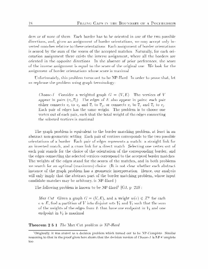
18 Filling Gaps in the Boundary of a Polyhedronders or of none of them. Each border has to be oriented in one of the two possibledirections, and, given an assignment of border orientations, we may accept only in-verted matches relative to these orientations. Each assignment of border orientationsis scored by the sum of the scores of the accepted matches. Naturally, for each ori-entation assignment there exists the inverse assignment, where all the borders areoriented in the opposite directions. In the absence of prior preferences, the scoreof the inverse assignment is equal to the score of the original one. We look for theassignment of border orientations whose score is maximal.Unfortunately, this problem turns out to be NP-Hard. In order to prove that, letus rephrase the problem using graph terminology:Choose-1. Consider a weighted graph G = (V;E). The vertices of Vappear in pairs (vi; vi). The edges of E also appear in pairs: each paireither connects vi to vj and vi to vj , or connects vi to vj and vi to vj.Each pair of edges has the same weight. The problem is to choose onevertex out of each pair, such that the total weight of the edges connectingthe selected vertices is maximal.The graph problem is equivalent to the border matching problem, at least in anabstract non-geometric setting. Each pair of vertices corresponds to the two possibleorientations of a border. Each pair of edges represents a match: a straight link foran inverted match, and a cross link for a direct match. Selecting one vertex out ofeach pair stands for the choice of the orientation of the corresponding border, andthe edges connecting the selected vertices correspond to the accepted border matches.The weights of the edges stand for the scores of the matches, and in both problemswe search for an optimal (maximum) choice. (It is not clear whether each abstractinstance of the graph problem has a geometric interpretation. Hence, our analysiswill only imply that the abstract part of the border matching problem, whose inputcandidate matches may be arbitrary, is NP-Hard.)The following problem is known to be NP-Hard1 [GJ, p. 210]:Max Cut. Given a graph G = (V;E), and a weight w(e) 2 Z+ for eache 2 E, �nd a partition of V into disjoint sets V1 and V2 such that the sumof the weights of the edges from E that have one endpoint in V1 and oneendpoint in V2 is maximal.Theorem 2.5.1 The Max Cut problem is NP-Hard.1Originally, it was stated as a decision problem which turned out to be NP-Complete. Similarreasoning to that in the proof given here shows that the decision version of Choose-1 is NP-Completetoo.

2.5 Matching Border Portions g 19Proof: By a reduction from Maximum 2-Satis�ability [Ka]. 2Theorem 2.5.2 The Choose-1 problem is NP-Hard.Proof: By a reduction from Max Cut. Given an instance graph G = (V;E) of theMax Cut problem, we build a graph G� for the Choose-1 problem. For each vertexvi 2 V , we construct a pair of vertices v1i and v2i in G�. For each edge e between twovertices vi and vj, we construct a pair of edges in G�, which connect v1i to v2j and v2ito v1j , and assign them the weight w(e). The construction is linear in the size of theinput. It is trivial to verify that a selection of vertices in the Choose-1 problem whichyields maximal weight of the corresponding selected edges implies optimal partitionof the vertices in the Max Cut problem (where V1 is the set of all vertices vi for whichv1i was selected, and V2 is the complementary set), and vice versa. 2It is important to note that relaxing the requirement that the weights of the twoedges of the same pair are equal does not make the problem any easier. Theorem 2.5.2implies that the relaxed problem is NP-Hard too, or else the original Choose-1 prob-lem would not have been NP-Hard. But even without Theorem 2.5.2 we could provethat the relaxed problem is NP-Hard, by a reduction from the problem of �nding anIndependent Set with a maximal size in a graph.In practice, though, getting an inconsistent collection of candidate matches is veryrare (provided that we do not accept matches that are too short). This is becausethe boundary of real models is always intended to be orientable. In the rare caseswhere our algorithm erroneously produces a match that is wrongly directed, thisusually happens when the match is very short, and then the two match orientationsare suggested, thus overlap, and are therefore eliminated.It is trivial to decide whether the set of suggested matches is consistent or not.We do that in a DFS-like process on another graph, whose vertices are the connectedcomponents of the polyhedron boundary, and whose edges are the suggested matchesbetween them. We arbitrarily choose a vertex (a component) as the start of thesearch, and assign to it an arbitrary orientation; each traversed edge (match) impliesa consistent orientation of the newly visited component. All we have to do is to checkconsistency of all pairs of vertices connected by back-edges of the DFS. This step isapplied for each connected component of the new graph.If the set of suggested matches is not consistent, we use the following simpleheuristic. We maintain a collection of pairwise-disjoint sets of connected componentsof the polyhedron boundary, where the components in each set have been stitchedtogether by already accepted matches and are consistently oriented. Initially, eachconnected component of the polyhedron is put in a separate singleton set. In eachstep we examine one match, in decreasing score order. If the match connects betweencomponents of di�erent such sets, then we merge the two sets, (and if necessary, invertthe orientation of all the components of one set), and accept the match. In case the

20 Filling Gaps in the Boundary of a Polyhedronmatch connects between components of the same set, we accept the match only if itis consistent with the current component orientations; otherwise it is rejected.We implemented this heuristic using a disjoint-set data structure, originally pro-posed by Galler and Fischer [GF]. The only operation we had to add is the inversionof orientation of all the members of one set, if necessary, in merging two sets. We dothat as part of the regular makeset, �nd and link operations (as is the terminology ofTarjan [Ta1]), without increasing their asymptotic e�ciency. Instead of maintainingthe orientation of a component, we indicate (using one bit) whether it is consistentwith the immediate ancestor component in the rooted tree, which implements theset of components. At the beginning, we perform all the makeset operations, creat-ing sets which all contain only one component consistent with itself. Processing amatch suggestion requires two �nd operations. During the traversal of the path froma component to the root of its set, we also compute the consistency state betweenthe component and the root. Thus, if the match connects components of the sameset, we can directly conclude whether the match is consistent with the previous onesor not, and accept only consistent matches. If the match connects components ofdi�erent sets, we link the two sets, and reset the consistency bit of the componentwhich ceases to be a root. It now points to the other root, which has just become theroot of the merged set.Finally, in case one connected component of the polyhedron boundary has severalborders, we must orient them with consistent directions. This can be done simply byadding arti�cial \matches" between these borders, with scores which dominate thoseof real matches. Thus, their acceptance is guaranteed.We summarize below the complete procedure for pruning match suggestions:1. Add new match suggestions for each connected component of the polyhedronboundary which has several borders. These matches should de�ne consistentdirections to all the borders of a component, and should be scored higher thanevery original match suggestion (the scores are needed only if the set of matchsuggestions is not consistent).2. Check whether all the match suggestions are consistent. For this purpose builda graph Gm, where each connected component of the polyhedron boundary is avertex in Gm, and each match suggestion is an edge in Gm. Choose arbitrarilya vertex of Gm and assign an arbitrary orientation to it. Perform a depth-�rstsearch in Gm. For every edge of the search, assign an orientation to the newlyvisited vertex according to the match corresponding to the edge. For every back-edge of the search, check whether its corresponding match is consistent with thealready assigned orientations of its two incident vertices. If all the back-edgesare consistent, then accept all the match suggestions and go to step 5. Otherwiseproceed to step 3.

2.6 Filling the Gaps g 213. Sort all the match suggestions according to their decreasing score order. Con-struct (makeset) a singleton set for each connected component Ci of the bound-ary, where i goes from 1 to the number of connected components. Maintainfor each connected component its inconsistency with the root of its set, repre-sented as an external ag, and initialize it to be false. (We use inconsistency ags rather than consistency ags in order to simplify the computation of therelative consistency between nodes in the structures.)4. Process sequentially all the match suggestions in their decreasing score order.For each match suggestion between components Ci and Cj do the following:� Find the set Ski (Skj ) which contains the connected component Ci (Cj).Denote its root by C�i (C�j ). Recompute the inconsistency of Ci (Cj)with respect to C�i (C�j ), as the exclusive or of the inconsistency agsencountered along the path from Ci (Cj) to C�i (C�j ).� If ki 6= kj then accept the match suggestion and link Ski and Skj . Assumewithout loss of generality that C�i now points to C�j as its parent. Resetthe inconsistency of C�i according to the accepted match.� If ki = kj and Ci and Cj are consistent (namely, their consistencies areeither both true or both false), then accept the match suggestion.� Otherwise, if ki = kj and Ci and Cj are not consistent , then reject thematch suggestion.5. Orient all the connected components in a way consistent with the acceptedmatches. Each connected component is now labeled to indicate whether itshould be inverted or not. If we reach this step from step 2, then each componentis classi�ed according to whether it is consistent with the root vertex of the DFSon Gm (or with its local root, if Gm is a forest). Otherwise, if we reach thisstep from step 4, then each component is classi�ed according to whether it isconsistent with the root of its set (again, there might be more than one set,if the accepted matches did not connect between all the components of thepolyhedron boundary). Inverting a component is performed by inverting thedirections of all the facets of the component.2.6 Filling the Gaps2.6.1 Stitching the Matching BordersEach match consists of two directed polygonal chains, which are very close to eachother in the three-dimensional space. We arbitrarily choose one end of the match,and \merge" the two chains as if they were sorted lists. In each step we have pointers

22 Filling Gaps in the Boundary of a PolyhedronFigure 2.3: Stitching a matchto the current vertices, u and v, in the two chains, and make a decision as to whichchain should be advanced, say v advances to a new vertex w. Then we add the newtriangle 4uvw to the boundary of the polyhedron (oriented consistently with theborders), and advance the current vertex (from v to w) along the appropriate chain.When we reach the last vertex of one chain, we may further advance only the otherone. This process terminates when we reach the last vertices of both chains.Several advancing rules were examined, and the following simplest one proved itselfthe best. Assume that the current vertices of the two chains are v1i and v2j , which arefollowed by v1i+1 and v2j+1, respectively. Then, if jv1i v1i+1j+jv2jv1i+1j < jv1i v2j+1j+jv2jv2j+1j,we advance the �rst chain; otherwise we advance the second chain. In other words,we advance so that the newly added triangle has smaller perimeter. Actually, we usedfor simplicity the squares of the distances, with equally good results. (This advancingrule is similar to that presented by Christiansen and Sederberg [CS].) This bears closeresemblance to the merging of two sorted lists, and turns out to produce reasonably-looking match triangulations. Figure 2.3 shows such a triangulation. We may furtherexamine the sequence of newly added triangles, and unify adjacent coplanar (or nearlycoplanar) triangles into polygons with larger sizes. Alternative advancing rules weredescribed by Ganapathy and Dennehy [GD] and by others.As an alternative to this merge simulation, we also examined match triangulationby the procedure described in the following Section 2.6.2. This method turned outto produce rather unaesthetic results, although it did yield a minimum-area triangu-lation.2.6.2 Filling the HolesAfter stitching the borders, we are likely to remain with small holes at the junctionsof cracks, as illustrated in Figure 2.5(g). These are 3-dimensional polygons, which

2.6 Filling the Gaps g 23are composed of portions of the borders that were not matched. This happens eitherbecause they do not meet the matching threshold, or because they belong to two ormore overlapping matches, and are thus removed.Identifying the holes is done in exactly the same way the original borders werelocated (see Section 2.4). In fact, these holes are the borders of the new boundaryafter the stitching phase. We found out that the best way to �x these holes was bya triangulation that minimizes the total area of the triangles. We, therefore, need tosolve the following problem:Given a 3-dimensional closed polygonal curve P , and an objective functionF de�ned on all triangles (called weight in the sequel), �nd the triangu-lation of P (i.e., a collection of triangles spanned by the vertices of P , sothat each edge of P is incident to only one triangle, and all other triangleedges are incident to two triangles each), which minimizes the total sumof F over its triangles.For this purpose, we closely follow the dynamic programming technique of Klincsek[Kl] for �nding a polygon triangulation in the plane, which minimizes the total sumof edge lengths. Let P = (v0; v1; : : : ; vn�1; vn = v0) be the given polygon. Let Wi;j(0 � i < j � n�1) denote the weight of the best triangulation of the polygonal chain(vi; : : : ; vj; vj+1 = vi). We apply the following procedure:1. For i = 0; 1; : : : ; n� 2, let Wi;i+1 := 0, and for i = 0; 1; : : : ; n � 3, let Wi;i+2 :=F(vi; vi+1; vi+2). Put j := 2.2. Put j := j + 1. For i = 0; 1; : : : ; n� j � 1 and k = i+ j letWi;k := mini<m<k[Wi;m +Wm;k + F(vi; vm; vk)]:Let Oi;k be the index m where the minimum is achieved.3. If j < n�1 then go to step 2; otherwise the weight of the minimal triangulationis W0;n�1.4. Let S := ;. Invoke the recursive function Trace with the parameters (0; n� 1).Function Trace (i; k):if i+ 2 = k thenS := S [ 4vivi+1vk;else do:a. let o := Oi;k;b. if o 6= i+ 1 then Trace (i; o);c. S := S [4vivovk;d. if o 6= k � 1 then Trace (o; k);od

24 Filling Gaps in the Boundary of a PolyhedronFigure 2.4: Minimum area triangulation of a holeAt the termination of the triangulation procedure, S contains the required trian-gulation of P . For our purposes, F(u; v; w) is taken to be the area of the triangle4uvw. In practice, in order not to totally ignore the aesthetics of the triangulation,we actually added a measure of \beauty" of a triangle to the weight function F , bymaking it slightly depend on the lengths of the triangle edges and on the spatialrelations between them. This avoided in most of the cases the creation of long skinnytriangles. Figure 2.4 shows an example of a triangulation of a hole.As in the stitching process, we may also test edges shared by newly added triangles,and unify groups of adjacent coplanar (or nearly coplanar) triangles into polygonswith larger sizes.2.7 Complexity AnalysisWe measure the complexity of the algorithm as a function of two variables: k, thesize of the input (say, the number of vertices of the original object), and n, the totalnumber of vertices along the border edges after the discretization. We denote thenumber of components by c, and the number of match suggestions by m. Naturally,c and m are expected to be signi�cantly smaller than n. We also denote the numberof triangulated holes by h, and the complexity (number of vertices) of the ith hole(i = 1; : : : ; h) by `i.We do not regard the computation of the connectivity (facets adjacency) infor-mation as part of our algorithm, since this should be part of the input. However, our

2.7 Complexity Analysis g 25preprocessing step generates this information, if needed, in O(k log k) time, whichis dictated by the sorting of the input vertices. The connected components of theboundary of the polyhedron can be found in time linear in k. The time needed for�nding their borders is also O(k). The discretization of the borders takes O(n) time.As in [HW], the voting step, if it uses a hash table, can be executed with expectedO(n) running time. This expected running time is due to the nature of hashing,and does not assume anything about the geometry of the input polyhedron to thealgorithm. Nevertheless, it assumes a reasonable choice of the proximity parameter", which should yield in average a constant number of output vertices for each range-searching query. Improper choice of ", say equal to the size of the whole object, willresult in �(n2) access operations to the hash table, but no matches will be identi�edin this case. (We could also achieve an O(n log2 n) deterministic running time byusing fractional cascading [Ch].) We infer the matches from the voting results also inO(n) time.Since choosing the maximal consistent set of matches is NP-Hard (at least in itsabstract non-geometric setting), we instead just check for consistency. As a DFS ina graph, it requires only O(m) time. If the collection of match suggestions is notconsistent, we invoke the heuristic described in Section 2.5.3, that takes O(m logm+m�(m; c)) time2. Stitching the borders, as merging sorted lists, is linear in theirsizes. Thus, the required time for all these operations is, again, O(n) (assuming thatm� n).Finding the remaining holes is now done in O(k+n) time, since this is the size ofthe new version of the object. The triangulation of each hole is done in time cubic in itssize. So the triangulation of all the holes requires O(Phi=1 `3i ) time. SincePhi=1 `i � n,it follows from the averages inequality that Phi=1 `3i � n3=h2. In the worst case, wherethere is a hole whose complexity is proportional to that of the whole input, this termis O(n3). Nevertheless, these cases are very unlikely in practice. Usually, the numberof holes is linear in the number of surfaces (and hence borders), and their sizes arevery small. The size of a hole is usually bounded by some constant (especially witha proper choice of the proximity parameters that control the voting process), so thisstep, although it is asymptotically ine�cient in the worst case, does not require morethan O(n) time in practice.To conclude, the whole algorithm runs on practical instances in average O(k +n) time, which is optimal. If we also count the connectivity computation in thepreprocessing, the algorithm runs in expectedO(k log k+n) time. In unrealistic cases,where the hole(s) are as complex as the polyhedral boundary itself, the running timemay climb to as high as O(k + n3) (or to O(k log k + n3), when we also compute theconnectivity).2�(m;n) is an extremely slowly growing functional inverse of Ackermann's function. For allpractical values of m and n, �(m;n) does not exceed a very small constant; cf. [Ta1].

26 Filling Gaps in the Boundary of a PolyhedronThe following section describes our rather comprehensive experimentation withthe algorithm. In all cases that we tried, the running time was indeed small, and thecost of the (theoretically expensive) hole-stitching step was invariably negligible.2.8 Experimental ResultsWe have implemented the whole algorithm on a Digital DECstation 5000/240 andon a Sun SparcStation II in C. The implementation took about two man months,and the software consisted of about 3,500 lines of code. We have experimented withdozens of CAD �les whose boundaries contained gaps, and obtained excellent resultsin most of the cases. These CAD �les were generated by various CAD systems,such as Euclid-IS (vendor: Matra Datavision), Unigraphics (McDonnell Douglas),Catia (IBM/Dassot), CADDS-4X (Computer Vision), ME (Hewlett Packard), Pro-Engineer (Parametric Technologies), and many others. We note that most of theproblems occurred when stand-alone computer programs translated curved objectsfrom neutral �le format, e.g. VDAFS [VDA] or IGES [NIST], into their polyhedralapproximations. Fewer problems appeared when the CAD systems performed thesame task, using a built-in function which converts the internal data into an output�le which contains a polyhedron description. The �les described industrial models,primarily parts and subunits of the automotive industry, which were extracted fromCAD systems for the fabrication of three dimensional prototypes. Most of the modelswere speci�ed in the STL [3DS] �le format, which is the de-facto standard in the rapidprototyping industry.The tuning of the parameters was very robust, and large parameter ranges pro-duced nearly identical results. We usually used 0.1 mm as the discretization parame-ter, and 0.5 mm for the voting threshold " (for models whose global size was between2 to 20 cm in all dimensions). We allowed up to two successive point mismatchesalong a match. A point-to-point match contributed the amount of 1=(d+ 0:1) to thematch score, where d was the distance between the two points. We considered onlymatch suggestions which received more than 10 votes and whose scores were above25:0. The triangle weight function F was taken to be 0:85A+ 0:05P + 0:10R, whereA was the area of the triangle, P was its perimeter, and R was the ratio between thelargest and the smallest of its three edges.All these parameters were user de�ned, but modifying them did not achieve anybetter results. Therefore, the program set these defaults for the parameters, exceptfor the voting threshold ". As noted above, this should be the user estimation of thephysical size of the gaps between the original surfaces. The success of the algorithmprimarily depended on a proper choice of ", which was rather simple, since a largeenough range of valid " setting produced adequate results. However, a too small "resulted in the loss of matches due to the lack of votes. On the other hand, a too large "

2.8 Experimental Results g 27(a) (b) (c) (d)(e) (f) (g) (h)Figure 2.5: A synthetic exampleresulted in a noisy voting table. This usually caused \intuitively-correct" matches notto have scores su�ciently larger than incorrect match suggestions. Even when suchintuitive matches were identi�ed, they overlapped with erroneous match suggestionsand were therefore eliminated. In all cases, too many unmatched border portionswere passed to the triangulation step. When the remaining holes were not local(with respect to the geometric features of the original model), their triangulationsconstructed new surfaces far beyond the intention of the model designer. Nevertheless,all these problems were eliminated by a proper choice of ".Figure 2.5(a) shows a synthetic example of an object similar to a cube, whoseboundary was broken into eight components, none of which is planar. Figure 2.5(b)shows the same object in a wire-frame representation. Figures 2.5(c,d) show theobject after the whole repairing process. Figures 2.5(e,f,g,h) show the di�erent stepsof the algorithm. The borders are shown in (e), the matches (after stitching theborders) are shown in (f), the remaining holes are shown (with the same perspectiveview) in (g), and their minimal area triangulations are shown in (h).Figure 2.6(a) shows another synthetic example, where a sphere contains very smallholes in the poles. Figures 2.6(b,c) show one of the poles, before and after triangu-lating the hole, respectively.Real examples turned out to be simpler, since the matching borders were muchlonger and closer than in the synthetic examples. Many polyhedral approximations ofsurface-modeling objects were repaired using the algorithm described in this chapter.A typical example (a hollowed trimmed box) is shown in Figure 2.7. The front

28 Filling Gaps in the Boundary of a Polyhedron(a) (b) (c)Figure 2.6: A sphere with perforated poles

(a) (b) (c)(d) (e)(f) (g)Figure 2.7: A real example

2.8 Experimental Results g 29(a) (b)Figure 2.8: Three intersecting \drums"side of the object is shown in Figure 2.7(a), whereas its bottom side is shown inFigure 2.7(b). The borders are shown in Figure 2.7(c), and all of them are matched,leaving only six holes. Since the holes are so small, they appear as dots in this scale.Figures 2.7(d,e) are closeups of the area near the left intersection of the two pairsof full circular borders (as seen in the lower part of (c)), before and after stitching,respectively. Figures 2.7(f,g) are closeups of a hole before and after its minimum-areatriangulation.Figures 2.8 and 2.9 show two more real cases. Figure 2.8(a) shows two intersecting\drums", where a third part protrudes out of the near drum. Figure 2.8(b) is a closeupof two tiled matches (from a di�erent point of view), in a wire-frame representation.Figure 2.9(a) shows a complex of �ve open hollowed cylinders. One long gap separatesbetween the inner and outer surfaces of the complex. Two portions of the singleborder, that completely bounds this gap, were fully matched and tiled. Figure 2.9(b,c)are closeups of the tiled match.Figure 2.10 shows three more real examples which our algorithm fully cured. Avoting table which corresponds to a typical match is shown in Figure 2.11. The solidcurve represents the number of votes (as a function of the shift); it is superimposedby the dotted curve, which represents (in a di�erent scale) the score of each shift.The two peaks in the graphs indicate two di�erent matches between portions of thesame pair of borders. We summarize the performance of our implementation on allthe examples described above in Table 2.1. All the time measurements were taken ona Digital DECstation 5000/240.

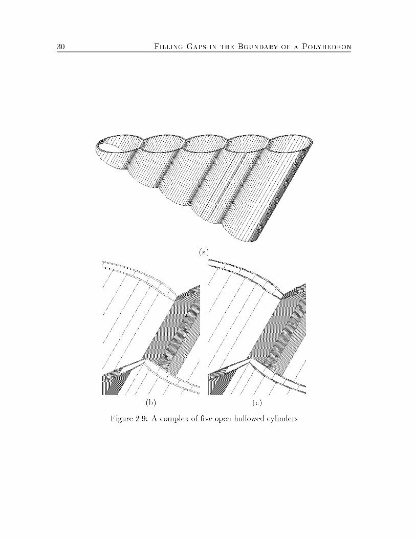
30 Filling Gaps in the Boundary of a Polyhedron

(a)(b) (c)Figure 2.9: A complex of �ve open hollowed cylinders

2.8 Experimental Results g 31

(a) Impeller (b) Drawer(c) AdapterFigure 2.10: Three more real examples

32 Filling Gaps in the Boundary of a PolyhedronComplexity Border HoleModel Vertices Edges Facets Borders Points Matches Holes PointsSynthetic 45 111 37 8 278 18 12 61Sphere 432 2,448 816 2 48 0 2 48Box 1,545 3,244 609 32 5,305 30 6 47Drums 826 1,712 372 19 3,106 35 22 233Cylinders 1,571 3,132 783 1 1,592 1 0 0Impeller 7,284 43,635 14,545 11 47 0 11 47Drawer 458 2,817 939 1 203 1 0 0Adapter 6,539 44,682 14,894 27 84 0 27 84Time (Seconds)Model Stitching Triangulation TotalSynthetic 0.48 0.20 0.68Sphere 0.13 0.06 0.19Box 10.14 0.60 10.74Drums 5.95 0.20 6.15Cylinders 3.60 0.00 3.60Impeller 1.12 0.35 1.47Drawer 0.24 0.00 0.24Adapter 2.48 0.06 2.54Table 2.1: Performance of the gap-�lling algorithm

2.9 Conclusion g 33Number of votes Score

0 3 6 9 12 15 18 21 24 27 30 33 36 39 42 45 48 51 54 57 60 63 66Shift

0

5

10

15

20

25

30

35

40

45

50

55

60

65

70

75

Vot

es &

Sco

re

Figure 2.11: A voting table of a typical match2.9 ConclusionWe have proposed in this chapter an algorithm for solving a practical problem, namelythe detection and repair of gaps in the boundary of a polyhedron. This problem arisesquite frequently in practice, during the computation of polyhedral approximations ofCAD models, whose boundaries are described using curved entities of higher levels.We applied several techniques in our solution. First, we used a partial curvematching technique, adapted from computer vision and based on geometric hashing,for identifying matching border portions. Then we chose a (nearly) maximal consis-tent set of match candidates, and stitched them together. Finally, we identi�ed theremaining holes and employed a minimum area triangulation of 3-D polygons in orderto �ll them.This method can be applied to other geometric problems, where portions of 3-dimensional polygonal curves should be matched. In the next chapter we presentan extension of it to the problem of piecewise linear interpolation between parallelpolygonal slices.

Chapter 3Piecewise-Linear Interpolationbetween Polygonal Slices3.1 IntroductionThe problem of reconstructing the boundary of a solid object from a series of parallelplanar cross-sections has attracted much attention in the literature during the pasttwo decades. The main motivation for this problem comes from medical imagingapplications, where cross-sections of human organs, such as bones, tumors and tissues,are obtained by CT (Computed Tomography) or MRI (Magnetic Resonance Imaging)apparata. These cross-sections, hereafter called slices, are the basis for interpolatingthe boundary surface of the organ. The interpolated object can then be displayed ingraphics applications, or (more recently) even manufactured by an NC (NumericallyControlled) or an RP (Rapid Prototyping) machine. Another motivation for thisproblem is the non-destructive digitization of objects: after an object is scanned by anecho-graphic or an X-ray apparatus, the obtained slices are used for the reconstructionof the original object. Yet another motivation is the reconstruction of a 3-dimensionalmodel of a terrain from topographic elevation contours.Many solutions were suggested for the pure raster interpolation. These usuallyhandle two raster images, where each pixel is either white or black, or assigned a greylevel taken from a �xed range. The interpolation produces one or more intermediateraster images, which smoothly and locally turn the �rst image into the second one.Then, the bounding surface is detected using other methods, such as edge detectiontechniques, for identifying places of transition from the inside to the outside of theobject. In the grey level case, these methods include some thresholding mechanismwhich decides which levels are `inside' the object and which are not. Cline et al.[CLLC, LC] attempted to convert directly the voxel data into a polyhedral surface,suggesting the marching cubes technique, which produced very small triangles whose35

36 Piecewise-Linear Interpolation between Polygonal Slicessize was roughly the same as that of the input voxels.Many other solutions, including the approach taken in this chapter, assume thatthe interpolation is preceded by an edge-detection process, which is invoked for eachof the slices. Thus, each slice is then assumed to be represented by a hierarchy ofnon-crossing contours, each being a closed simple Jordan curve, which represent theboundaries between \material" and \non-material" areas; in general, the depth andbreadth of this hierarchy is not restricted, and a contour may enclose any number ofother contours, which themselves may enclose other contours, and so on. In practice,each contour is given as a discrete circular sequence of points along it, and we canthus regard it as a simple closed polygonal curve, whose vertices are the given points.Finally, we may also assume that the exterior, unbounded region in each planar slicerepresents \non-material" (the model is assumed to be bounded).Thus the problem that we face is: Given a series of parallel planar slices (whichwe will assume to be parallel to the xy-plane), each consisting of a collection of non-crossing, but possibly nested, closed and simple polygonal curves, with the aboveproperties, we want to reconstruct a polyhedral solid model whose cross sectionsalong the given planes coincide with the input slices. A natural simpli�cation ofthe problem, also taken in most earlier works, is to consider only a single pair ofsuccessive parallel slices, and to construct a solid model within the layer delimitedby the planes of the slices, which interpolates between the given slices. The union(or, rather, concatenation) of these models will give us a solution model for the fullproblem. (Admittedly, some smoothness might be lost in this simpli�ed approach.This, however, does not seem to be a serious problem in medical imaging, where twoadjacent slices often di�er a lot from one another, so smoothness considerations donot seem to have much in uence on the solution. Also, even the reduced problem wastoo di�cult to solve in full generality in earlier works|see below.)Before continuing, we should remark that the solution is not uniquely de�ned, andthe measure of `goodness' of a proposed solution is rather subjective and intuitive. Ofcourse, if each of the two slices consists of a single contour, and these contours roughly`sit above each other', then we expect the solution to be a single `drum-like' polytopewhose boundary consists of a circular sequence of triangles `wrapping around' thetwo contours; see Figure 3.1(a). (Welzl and Wolfers [WW] have proposed anothercriterion, that if the two contours are convex, then the solution should coincide withtheir convex hull.) However, even in the simple case of one contour in each slice, ifthe xy-projections of the two contours are far away from each other, it is not clearwhich is a better solution: to construct a highly slanted `pipe' that connects betweenthese contours (as in Figure 3.1(b)), or to regard the lower contour as the top cover ofsome pillar-like solid, and the upper contour as the bottom cover of another pillar-likesolid (as in Figure 3.1(c)). The choice of a solution can become much more arbitraryin more involved cases.We thus consider the problem of interpolating between two successive slices, each

3.1 Introduction g 37Figure 3.1: Contour association and tilingconsisting of a collection of simple closed polygonal contours in any hierarchy ofnesting. We assume only that the data is valid, i.e. no two contours of the sameslice cross each other (but they may touch). Hence, we skip the usual step of edgedetection in raster images, and assume that detected contours are already available.3.1.1 Previous WorkWe �rst review the fairly extensive literature on this problem. Most of the earlierworks only studied the variant where each slice contains only one contour. In thesequel we denote it as the one-to-one case, as opposed to the one-to-many and themany-to-many cases. These studies either sought a global optimization of some ob-jective function, or settled with a local tiling-advancing rule, after the tiling startingpoints at the two contours were somehow determined, e.g. the closest pair of verticesbetween the contours.The �rst solutions for this problem (that we are aware of) were proposed by Keppel[Ke] and by Fuchs, Kedem, and Uselton [FKU]. Keppel dealt with the simple case,where each slice contains only one contour, and implicitly assumed a high degree ofresemblance between them. After restating the problem in graph terminology, Keppelsought a minimum path in a weighted toroidal graph, which represented the tilingwhich yields the interpolating polyhedron with maximumvolume. Similarly, Fuchs etal. also dealt with the simple one-to-one case, and obtained, using a similar reduction

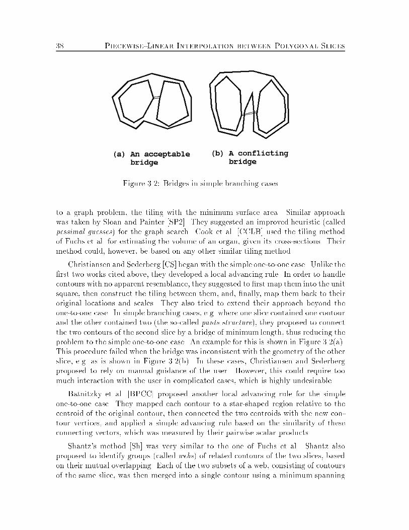
38 Piecewise-Linear Interpolation between Polygonal SlicesFigure 3.2: Bridges in simple branching casesto a graph problem, the tiling with the minimum surface area. Similar approachwas taken by Sloan and Painter [SP2]. They suggested an improved heuristic (calledpessimal guesses) for the graph search. Cook et al. [CCLB] used the tiling methodof Fuchs et al. for estimating the volume of an organ, given its cross-sections. Theirmethod could, however, be based on any other similar tiling method.Christiansen and Sederberg [CS] began with the simple one-to-one case. Unlike the�rst two works cited above, they developed a local advancing rule. In order to handlecontours with no apparent resemblance, they suggested to �rst map them into the unitsquare, then construct the tiling between them, and, �nally, map them back to theiroriginal locations and scales. They also tried to extend their approach beyond theone-to-one case. In simple branching cases, e.g. where one slice contained one contourand the other contained two (the so-called pants structure), they proposed to connectthe two contours of the second slice by a bridge of minimum length, thus reducing theproblem to the simple one-to-one case. An example for this is shown in Figure 3.2(a).This procedure failed when the bridge was inconsistent with the geometry of the otherslice, e.g. as is shown in Figure 3.2(b). In these cases, Christiansen and Sederbergproposed to rely on manual guidance of the user. However, this could require toomuch interaction with the user in complicated cases, which is highly undesirable.Batnitzky et al. [BPCC] proposed another local advancing rule for the simpleone-to-one case. They mapped each contour to a star-shaped region relative to thecentroid of the original contour, then connected the two centroids with the new con-tour vertices, and applied a simple advancing rule based on the similarity of theseconnecting vectors, which was measured by their pairwise scalar products.Shantz's method [Sh] was very similar to the one of Fuchs et al. Shantz alsoproposed to identify groups (called webs) of related contours of the two slices, basedon their mutual overlapping. Each of the two subsets of a web, consisting of contoursof the same slice, was then merged into a single contour using a minimum spanning

3.1 Introduction g 39tree of bridges. This method could also produce bridges that con icted with theother slice, as mentioned above. In those cases, Shantz proposed that the user directthe algorithm by adding arti�cial degenerate contours, that will force the minimumspanning tree to behave `nicely'. In addition, Shantz handled the cases where acontour of one slice did not appear to match any one of the other slice. This seemedto indicate the top cover or bottom cover of some feature of the solid, and thus thewhole contour was simply added to the construction as a new disconnected portion.Sloan and Hrechanyk [SH1] also dealt with the simple one-to-one case. Theircontribution was the suggestion to create arti�cial intermediate slices, in cases wherethe original ones were extremely di�erent. Then, each pair of successive slices wastreated by the previous algorithms. Ganapathy and Dennehy [GD] still dealt withthe one-to-one case. They proposed an advancing rule based on the so-called tensionof the surface.Wang and Aggarwal [WA] also dealt mainly with the simple one-to-one case.Based on the amount of contour overlapping, they decided whether to project acontour from one slice onto its matching counterpart from the other slice, connect thetwo contours, or none of these. The triangulation de�ning the reconstructed surfacebetween two contours was obtained using the known A� heuristic search algorithm.The underlying graph was similar to the graphs of Keppel and Fuchs et al., exceptthat the merit function used there aimed to minimize the total sum of edge lengths.Wang and Aggarwal also proposed to unify adjacent coplanar triangles, both in thesame layer (tiling between two slices) and in successive layers, in order to form fewerpolygons with larger complexities.A good survey on all the works cited so far is given by Sloan and Painter [SP1].They decompose each method into its building blocks, and compare the various meth-ods accordingly. They also describe a testbed for evaluating and comparing thesetechniques.Zyda, Jones, and Hogan [ZJH] made an attempt to handle the many-to-manycase. They attributed the contour interiors as high or low instead of specifyingtheir orientations. Their algorithm used these attributes, as well as bounding-boxoverlap analysis, in order to locate partial contour mapping. They tiled the matchingcontours the same way as Christiansen and Sederberg. The main limitations of theirmethod were its inability to handle any branching cases, and unsatisfactory results forpartially overlapping contours, as in Figure 3.5. Other limitations involved speci�cgeometries. However, they suggested solutions for these limitations, which might helpin certain cases, but which required some interaction with the user.Boissonnat [Bo1] presented a totally di�erent approach. He constructed the De-launay triangulation for each slice, projected one triangulation onto the other, andobtained a collection of tetrahedra, aiming to maximize the sum of their volumes.This was a considerable step towards handling the case where each slice has multiple

40 Piecewise-Linear Interpolation between Polygonal Slicescontours. Boissonnat mentioned three typical examples where his standard methodfailed to produce good results, thus requiring special treatment. The �rst examplecontained two overlapping contours but with considerable di�erences in their geom-etry. The second example consisted of two similar contours, where one of them alsocontained a hole polygon. And the last example showed a branching problem butwithout contour overlaps. Boissonnat suggested a correction scheme, which eitherchanged the geometry of one of the slices, or constructed one or two intermediateslices between the original ones. Boissonnat states [Bo1, p. 21]: \In our opinion, anymethod will fail when the measures are poorly conditioned", stipulating that no algo-rithm will be able to produce satisfactory results when the pair of slices are too muchdi�erent in the number of contours or in their geometries. Nevertheless, our algorithmhandles these cases (as well as considerably more complex ones) rather routinely andsuccessfully. Improvements and applications of the method of Boissonnat are givenby Boissonnat and Geiger in [BG, Ge].Kehtarnavaz and de Figueiredo [KD] �rst segmented the contours according tolocal curvature and torsion, and assigned characteristics values to the segments. Af-ter concatenating these segment characteristics into circular strings, they performedstring matching between these characteristic strings. Finally, they blended the con-tours by smooth functions, e.g. splines. They also dealt only with the simple one-to-one case. Similar ideas were presented by Kehtarnavaz, Simar, and De Figueiredo[KSD]. They used other features for contour segmentation, and used string matchingwith errors, allowing insertions and deletions in the matched strings.Ekoule, Peyrin, and Odet [EPO] developed special treatments for some of themultiple-contour cases. For the simple one-to-one case, where the two contours wereconvex, they suggested a local minimum edge-length heuristic as an advancing rule.When the contours were not convex, they �rst detected the convex and concaveportions of the contours, then projected the concave portions onto the convex hullsof the contours, and applied the previous method to the projections. This approachrelied on the hypothesis that the convex hulls of the two contours were similar in shapeand orientation. In the case of connecting one contour with multiple contours, theyproposed the creation of an intermediate slice, which contains only one contour|acombination of the convex hulls of the contours and edges connecting their centroids.This intermediate slice was then interpolated with the two original slices. Whenthe two slices contained more than one contour, they performed contour overlappinganalysis, and assumed that all the contours of every overlapping subset of contours,except one, were contained in one of the two slices, thus reducing to the previouscase.Meyers, Skinner, and Sloan [MSS] divided the problem into four subproblems,namely the correspondence problem, the tiling problem, the branching problem, andthe surface �tting problem. They focused their attention on the correspondenceand on the branching problems, and assumed that good solutions to the two other

3.1 Introduction g 41problems already existed. For the correspondence problem, Meyers et al. either usedoverlapping analysis based on the assembly of elliptical cylinders from the contours,or computed the Euclidean minimum spanning tree of the graph constructed for thecontours. For the branching problem, they formed a composite contour from thebranching contours, thus reducing to the simple one-to-one case. They also suggesteda special treatment of a canyon between contours, but did not specify how theyautomatically determined this case and identi�ed the canyon endpoints.Welzl and Wolfers [WW] provided an angle criterion for tiling between two poly-gons, with no branching. This criterion satis�es the following conditions: (i) if thetwo polygons are convex, then the reconstruction coincides with the convex hull oftheir union; and (ii) if one of the polygons is a homothetic copy of the other one(obtained by a parallel projection of the other polygon from some stationary pointp), then the reconstruction is the portion of the cone de�ned by either polygon withapex p, which lies between the two planes containing the polygons. We note thatour method does not necessarily satisfy any of the two conditions above. However,they are theoretical and are rarely practical. Welzl and Wolfers also showed that anysurface that violates their angle-consistency criterion must be self-intersecting.Finally, Gitlin, O'Rourke, and Subramanian [GOS] prove that it is not alwayspossible to �nd an interpolating polyhedron between two polygons, that lie in twoparallel planes. That is, any attempted interpolation produces a self-intersectingsurface. This result holds only when the interpolating triangles are all assumed toconnect between the two polygon vertices, i.e. to have two vertices taken from onepolygon and the third from the other polygon. We do not assume this in our approach,and we indeed get a non-intersecting interpolation when we apply our algorithm ontheir example.Two comprehensive reviews of many of the works on reconstructing 3-dimensionalobjects from cross-sections are given by Schumaker [Sc] and by M�uller and Klingert[MK, x7]. The �rst review is not restricted to piecewise-linear constructions based onpolygonal slices, but also refers to parametric and tensor representations of contours,and describes volumetric and surface approaches.3.1.2 Our ApproachWe propose a new approach to the interpolation problem. Our algorithm handleswell slices with multiple contours, and does not rely on any resemblance between theslices. We accept slices which contain any number of contours, arbitrarily di�erentin their geometries. The xy-projections of contours of di�erent slices may arbitrarilyoverlap; we do not make any distinction in the treatment of contours which fullyoverlap, partially overlap or do not overlap at all. Many of the previous works, suchas [Ke], [FKU], [SH1] and [GD], either prohibit the creation of triangles in the same

42 Piecewise-Linear Interpolation between Polygonal SlicesFigure 3.3: Matching contour portionsslice, or speci�cally de�ne steps where this action is allowed. We do not make adistinction between triangles which connect the two slices and those which totally liewithin a single slice. Generally speaking, our algorithm is based on an analysis of theresemblance between the two slices. Thus, we separately treat similar contour portionsthat are matched between the two slices, and then treat the remaining portions thatdo not match. We refrain from creating arti�cial bridges between contours that mightcon ict with the geometry of the other slice, as already noted in [Sh] and others. In theonly case where we construct such bridges, they are guaranteed not to con ict with thegeometry of the other slice, i.e. not to intersect the projection of any other contour.We do not have to introduce intermediate slices. As suggested in [WA], we mayoptionally unify adjacent coplanar triangles as they are produced, in order to remainwith fewer polygons, though with larger sizes. To recap, our algorithm appears toovercome most of the technical di�culties that hampered the performance of previoussolutions, it treats data in full generality, and the extensive experimentation that wehave conducted indicates that it performs very well on complicated large-size data.We regard our algorithm as a signi�cant step in the solution of this problem, especiallyin the multiple-contours case. For an illustration of the performance of our algorithmon real complex examples, see Figures 3.19, 3.20, 3.22, and 3.23.Here is a brief overview of our algorithm. We �rst match similar contour portionsbetween the two slices (e.g. the upper arcs pq and p0q0 in Figure 3.3). Then we`stitch' (or `tile') each pair of matched contour portions by a sequence of adjacenttriangles forming a `band' between the portions. With some care, if we take theunion of the original contours and new bands, and cancel out duplicate edges, weobtain a collection of closed spatial polygonal curves, each of which may be composedof pieces of contours on both slices and of some edges of the connecting triangles.Moreover, our matching procedure essentially guarantees that the xy-projections ofthese curves are pairwise disjoint, although they may be nested within each other.If no nesting occurs, we simply triangulate each of these spatial polygons, using asimple dynamic programming approach, which roughly aims to minimize the totalarea of the triangulation. If nesting occurs, we take one polygon P with all polygons

3.2 Statement of the Problem g 43P1; : : : ; Pk whose xy-projections are directly nested within that of P , and apply aminimum spanning tree procedure that introduces edges connecting between thesepolygons and yielding an xy-projection which is simply connected, so we can thenproceed to triangulate the resulting polygonal curve, as above. See Figure 3.4 for anillustration. More details of all these steps will be given later in this chapter.For the purpose of identifying matching portions of the contours we use (as foridentifying matching border portions in the gap-�lling problem|see Chapter 2) apartial curve matching technique, based on the geometric hashing scheme (see Sec-tion 1.3). In the gap-�lling variant no motion of one curve relative to the other wasallowed, and we had to match 3-dimensional curves. The matching that we needfor the current problem uses a similar technique, and is even simpler, because ourmatched curves lie on a pair of parallel planes.This chapter is organized as follows. In Section 3.2 we give a more precise de�ni-tion of the problem. Section 3.3 presents an overview of the algorithm (more detailedthan the one given above). The later sections describe in detail the various phases ofthe algorithm. Section 3.4 describes the data acquisition phase, Section 3.5 describesthe matching of contour portions, and Section 3.6 describes the actual surface recon-struction. In Section 3.7 we analyze the complexity of the algorithm, and Section 3.8presents experimental results. We end in Section 3.9 with some concluding remarks.3.2 Statement of the ProblemWe are given a pair of parallel planar slices, assumed, with no loss of generality, to beparallel to the xy-plane, and to lie at heights z = z1 and z = z2, respectively. Eachslice consists of a list of closed and simple polygonal contours, which do not intersecteach other, where each contour is given as a circular list of vertices, each speci�ed byits (x; y) coordinates.The containment hierarchy of the contours may be omitted; in this case we com-pute it ourselves. Contours of the root level (not contained in any other contour) areassigned level 0, their holes are assigned level 1, etc. Thus, every even level consistsof contours whose interior, in a su�ciently small neighborhood of the contour, is the\material", and every odd level consists of contours whose interior, su�ciently nearthem, is the \non-material" (this follows from the assumption that the solid to bereconstructed is bounded). We orient each contour so that, when viewing the contourfrom above, the material lies to the right of the contour (thus all even-level contoursare oriented in the clockwise direction, when viewed from above, and all odd-levelcontours are oriented in the counter-clockwise direction). Since the orientations ofthe input polygons are arbitrary, we may have to re-orient them in these consistentdirections. The construction of the hierarchy and of the contour orientations is easilyperformed, using e.g. a line-sweep procedure in each slice. We remark that we need to

44 Piecewise-Linear Interpolation between Polygonal Slicescompute the contour hierarchy only to obtain the consistent orientation of contours;the hierarchy itself is not used in the algorithm.The main problem addressed in this chapter is to construct a polyhedral solidobject K, bounded by an orientable manifold and contained in the layer z1 � z � z2,so that its intersection with the plane z = z1 coincides with the material regions ofthe corresponding slice, and similarly for z = z2. We have already remarked thatsuch a K, and even its topology, is not necessarily unique, and we require that thealgorithm produce a model that is intuitively `good'. It seems hard to come up witha rigorous formulation of `goodness', and so we will not attempt it. After presentingour algorithm, we will comment on its performance on certain examples, and try toconvince the reader that its output is indeed `good'.Note that, in order to construct a closed volume, we have to include in the bound-ary of K the material regions of the two slices. In the original problem we are usuallygiven a series of more than two parallel slices. In this case it su�ces to `close' K bythe material regions of only the highest and lowest slices; see below for a more preciseelaboration of this comment.3.3 Overview of the AlgorithmOur proposed algorithm consists of the following steps:1. Data acquisition:� Orient all the contours in each slice in consistent directions, as explainedabove. If the input does not include this information, compute the contournesting hierarchy in each slice, and use it to obtain the desired orientations.2. Matching contour portions:� Discretize each contour polygon into a cyclic sequence of vertices, so thatthe arc length between each pair of consecutive vertices is equal to some(small) given parameter.� Vote for contour matches. Each pair of distinct vertices of the discretizedcontours, one on each slice, whose mutual horizontal distance (that is, theirdistance after projecting one slice onto the other) is below some thresholdparameter, contributes one vote. The vote is for the match between thesetwo contours with the appropriate shift, which maps one of these verticesto the other.� Transform the resulting votes into a collection of candidates of partialcontour matches.

3.4 Data Acquisition g 45� [Optional ] Discard, for storage e�ciency, all the points added in the dis-cretization step, except for the endpoints of the matches.3. Reconstructing the surface:� Stitch together each pair of contour portions that have been matched inthe above step, by adding triangles that connect between these portions.The new triangles are oriented consistently with the contours.� Combine the remaining contour edges into spatial cycles (called clefts),obtained by taking the union of the contour edges in both slices and of theedges of the stitching triangles, and by canceling out duplicate, oppositely-oriented edges. When projected onto the xy-plane, these cycles do notintersect each other (except in very rare and unrealistic cases, which neverarose in our experimentation). Find their nesting hierarchy, and, for eachcleft C, construct, if necessary, a system of straight `bridges' that connectbetween C and its holes (immediate children in the hierarchy), so as toturn them into a single cycle, which now replaces the cleft C.� Triangulate the resulting 3-D clefts, using (a variant of) a 3-D minimumarea triangulation technique.The various steps of the algorithm are illustrated in Figure 3.4. Figure 3.4(a) showsa pair of slices in a branching situation. The lower slice contains one contour (denotedby S1), and the upper slice contains three contours (denoted by S2). Figure 3.4(b)shows the tiling of the three matches found between these two slices. Figure 3.4(c)shows the remaining clefts, which form a shallow hierarchy of nested polygons. Fig-ure 3.4(d) shows the clefts after the hole elimination step, and their minimum-areatriangulations are shown in Figure 3.4(e). The �nal surface reconstruction is shownin Figure 3.4(f).The following three sections describe the algorithm steps in detail.3.4 Data AcquisitionThis step has already been described in some detail earlier in the chapter. The actualdata consists of a sequence of slices, all in the same �le or each in a separate �le.Recall that each slice consists of a hierarchy of contours, i.e. a forest of closed simplepolygons, where a parent polygon fully encloses all its children, and no other contouris enclosed in the parent polygon and encloses one of its children. Each slice is alsomarked by its height along the z-axis; thus every vertex is speci�ed by its threecoordinates.We are not interested in the nesting hierarchy itself, but only in the consistentpolygon orientations that it implies, in the manner described above. In many cases,

46 Piecewise-Linear Interpolation between Polygonal Slices

Figure 3.4: The di�erent steps of our algorithm (view from above)

3.5 Matching Contour Portions g 47the preprocessing edge-detection algorithm already orients all the polygons in thecorrect directions. When we cannot rely on that, our system invokes a standard line-sweep algorithm, as a preprocessing step, for computing the hierarchy and re-orientingall the polygons in the correct directions.The internal representation of the contours that our system uses is the quad-edgedata structure described by Guibas and Stol� [GS]. This is done for maintaininge�ciently the constructed polyhedral boundary of the interpolating solid object.In what follows, unless otherwise speci�ed, we restrict our attention to a singlepair of successive slices, and describe the manner in which the algorithm constructsan interpolating solid within the layer delimited by the slices.3.5 Matching Contour Portions3.5.1 Contour DiscretizationThis step is identical to the one described in Section 2.5.1. Each contour polygon isre�ned and discretized into a cyclic sequence of points. This is done by choosing somesu�ciently small arc length parameter s, and by generating equally-spaced points,at distance s apart from each other (along the polygon boundary). In analogy withthe works on object recognition cited in Section 1.3, we may regard the resultingdiscretization as footprints of the contours. We need to choose s so that it is muchsmaller than (a) the length of any original edge of any contour, and (b) the minimumstraight distance between any pair of contour points which lie on di�erent contours(on the same slice) or lie on the same contour and their distance along the contour issu�ciently large.3.5.2 Voting for Contour MatchesThis step is very similar to the one described in Section 2.5.2. We �rst try to matchpairs of portions of contours, where each portion in a pair belongs to a di�erentslice. These matches aim to detect regions of similarity between the boundaries ofthe interpolating object along the two slices. Naturally, contour portions which aresimilar in the two slices must have similar sequences of footprints. Thus, our nextgoal is to search for pairs of su�ciently long subsequences that closely match eachother. In our approach, two subsequences (pi; : : : ; pi+`�1) and (qj; : : : ; qj+`�1) are saidto closely match each other, if, for some chosen parameter " > 0, the number ofindices k for which kpi+k � qj+kk � " is su�ciently close to `. (Here the norm k � kis the Euclidean distance between the xy-projections of the points.) We denote theterm (j � i) as the relative shift between the two contours, by which the indexing

48 Piecewise-Linear Interpolation between Polygonal Slicesof the appropriate portion of the �rst contour has to be aligned with its counterpartfrom the second contour. We perform the following voting process, where votes aregiven to good point-to-point matches.The contours are given as cyclic ordered sequences of vertices. We break each cycleat an arbitrary chosen vertex, thus making it a linear rather than cyclic sequence.All the vertices of the lower slice are preprocessed for range-searching, so that, foreach vertex v of the upper slice, we can e�ciently locate all the vertices of the lowerslice that lie in some "-neighborhood of (the xy-projections of) v. As in the gap-�llingproblem (see Section 2.5.2), we have used a simple heuristic projection method, whichprojects the vertices onto each of the x- and the y-axes, and sorts them along eachaxis. Given a query "-neighborhood, we also project it onto each axis, retrieve thetwo subsets of vertices, each being the set of vertices whose projections fall inside theprojected neighborhood on one of the axes, then choose the subset of smaller size, and�nally test each of its members for actual containment in the query neighborhood.Again, this method, while ine�cient in the worst case, works very well in practice.The positions along a contour sequence c, whose length is `c, are numbered from0 to `c� 1. Assume that the querying vertex v is in position i of contour sequence c1.Then, each vertex retrieved by the query, which is in position j of contour sequencec2, contributes a vote for the match between contours c1 and c2 with a shift equal tos = (j� i) (mod `c2 ). We compute the shift modulo the length of the second contourso that we can easily retrieve later also the matched vertex, which is in position (i+s)(mod `c2) of contour c2.Obviously, matches between long portions of contours are re ected by a largenumber of votes for the appropriate shift between the matching contours. Since theremight be small mismatches between the two portions of the matching contours, or thearc length along one portion may not exactly coincide with the arc length along theother portion, it is most likely that a real match will be manifested by a signi�cantpeak of few successive shifts in the graph that plots the number of votes betweentwo contours as a function of the mutual shift (the same approach was taken in thegap-�lling algorithm of Chapter 2). Figures 3.13(a,b) show two such graphs, whichcorrespond to the two matches in the example shown in Figure 3.12. The high peakscorrespond to the correct shift values of the matches. Note that there might beseveral peaks in the same graph. This implies that there are several good matches,with di�erent alignments, between the same pair of contours.Keeping track (for each peak) of the portions of the contours which voted forthis alignment, we can infer the endpoints of the corresponding match (or matches)between these two contours. We extend the matches as much as possible, based onthe neighborhood of the peak, allowing sporadic mismatches, insertions or deletionsof points within the matched portion, up to some speci�ed limits. We achieve this bymaintaining for each possible match candidate m = (c1; c2; s) (for a pair of contoursc1, c2 and a relative shift s between them) the closest pair of points (one of c1 and one

3.5 Matching Contour Portions g 49of c2), which voted for it. We consider m as a match candidate only if the numberof votes for it is larger than all the possible matches of the form m = (c1; c2; s+ n),where 1 � jnj � M . That is, s is the best shift in a 2M -neighborhood of itself. For�nding the endpoints of the match candidate, we start with the closest pair of points(one on each contour), and traverse c1 and c2 from these points in both directions,collecting other pairs of matching points (with the same shift), and stopping as soonas we encounter � successive mismatches, where � is typically a small constant. Notethat the match itself can be circular, on one or both contours.Note that this procedure will only match contour portions that are consistentlyoriented. This is important, since it guarantees that the material region lies on thesame side of the two contours, thus implying that if we stitch the gap between thesetwo contours, we get a proper portion of the boundary of a possible interpolatingsolid.Also note that, as in the gap-�lling algorithm of Chapter 2, the " parameter forthe range-searching queries is not a function of the input. It is rather our a prioriestimation of the physical size of the di�erence between similar contour portions ofthe two slices.In some cases small portions of the contours are included in more than one candi-date match. This usually happens at the connection between two di�erent matches,involving the same contour on one slice and di�erent contours on the other. We simplyeliminate those portions common to more than one signi�cant candidate match.3.5.3 Accepting Match CandidatesEach match is given a score. The score may also re ect, in addition to the number ofvotes for the appropriate shift, other quality measures (such as the closeness of thevertices on the two matching contour portions). We chose our scoring function to bePi 1=(di+0:1), where i runs over all the voting pairs of points given to the match, anddi is the horizontal distance between the two points (as de�ned in Section 3.3). Wealso set minimum values for the number of votes and for the score that an acceptedmatch should have. Our setting of these parameters is described in Section 3.8.Unlike our gap-�lling algorithm of Chapter 2, where a similar voting process hasbeen used, but in accordance with all the works on object recognition cited in Sec-tion 1.3, we do not have to ensure any global consistency of orientation between allthe candidate matches. This is already implied by having correct contour directionsin both slices. After discarding the small match overlaps, if any, we are left with acollection of matches between similar contour portions of the two slices.The most important goal, which we have to achieve when tuning the parameterswhich control the detection of matches, is that every intersection between the xy-projections of any pair of contours, one from each slice, will lead to a match between

50 Piecewise-Linear Interpolation between Polygonal SlicesFigure 3.5: Intersecting contours with no long matching portionsthe corresponding contours, although it might be very short. This will ensure thatthere will be at least one match between each pair of overlapping contours (namely,contours with intersecting xy-projections), even if the relative amount of overlap isvery small.This property is crucial for the successful performance of the second phase ofour algorithm, described in Section 3.6.2. It ensures that the xy-projections of theunmatched contour portions, hence also of the spatial cleft cycles formed in the secondphase, do not intersect anywhere.We achieve this by accepting very short match candidates (even of length 2 or 3),as long as their quality �ts our bounds. We have to make sure that the discretizationparameter is su�ciently small with respect to the voting threshold and with respectto the smallest contour feature size, as described above, in order not to miss contourintersections. An extreme example is shown in Figure 3.5, where four short matchesare indeed found between the two contours.3.6 Reconstructing the Surface3.6.1 Stitching the MatchesThe stitching method is basically the one described in Section 2.6.1 for the gap-�lling problem, except for minor di�erences. Each match consists of two directedpolygonal chains, whose xy-projections are very close to each other. We arbitrarilychoose one end of the match, and `merge' the two chains as if they were sorted lists

3.6 Reconstructing the Surface g 51Figure 3.6: Tiling a matchof numbers. In each step of the merge we have pointers to the current vertices, u andv, in the two chains, and make a decision as to which chain should be advanced, sayv advances to a new vertex w. Then we add the new triangle 4uvw to the boundaryof the constructed polyhedron, and advance the current vertex (from v to w) alongthe appropriate chain. When we reach the last vertex of one chain, we may furtheradvance only the other one. This process terminates when we reach the last verticesof both chains.The triangles that we create are oriented consistently with the contours. Toachieve this, we invert the orientation of all contour polygons of one slice, say thelower one. If the base of a triangle lies on the upper slice, the triangle is oriented sothat its base is oppositely directed to the upper contour direction, and if the base lieson the lower slice, the triangle is oriented so that its base is directed in the originalorientation of the lower contour, i.e. opposite to the inverted lower contour. Thus,every edge shared by two tiling triangles, or by a tiling triangle and a contour, appearsin opposite directions, as should be expected from the reconstructed boundary of thepolyhedron. (This contour-inversion step is also useful when we have more than twoslices and we need to concatenate the reconstructed polyhedra in the layers betweenthem. The inversion implies that each \material" polygon in any intermediate sliceappears twice, in opposite orientations, so that, by canceling out these appearances,we obtain an overall solid whose boundary is consistently oriented.) Figure 3.6 showsthe directions of the (bases of the) tiling triangles.As in the gap-�lling problem, several advancing rules were examined, and thesame rule used in Chapter 2 proved itself the best in this case too. Speci�cally,

52 Piecewise-Linear Interpolation between Polygonal Slicesassume that the current vertices of the two chains are v1i and v2j , which are followedby v1i+1 and v2j+1, respectively. Then, if jv1i v1i+1j + jv2jv1i+1j < jv1i v2j+1j + jv2jv2j+1j, weadvance the �rst chain; otherwise we advance the second chain. In other words,we advance so that the newly added triangle has smaller perimeter; actually, forprogram e�ciency, we eventually used the squares of the distances, with equallygood results. This bears close resemblance to the merging of two sorted lists, andturns out to produce reasonably looking triangulated boundary patches between thematched contour portions. Figure 3.6 shows such a triangulation. We may alsofurther examine the sequence of newly added triangles, and unify adjacent coplanar(or nearly coplanar) triangles into polygons with larger sizes.As an alternative to this merge simulation, we also examined, as in Chapter 2,match triangulation by the more involved procedure described in Section 3.6.2. Thismethod turned out to produce in practice rather unaesthetic results, although ityielded a minimum-area triangulation between the matched contours.3.6.2 Filling the CleftsAfter tiling the matching contour portions, we remain with the unmatched portions.These, combined with the extreme edges of the tiling sequences, form a collectionof closed 3-D polygons, which we refer to as clefts. These clefts are similar to theremaining holes in the gap-�lling problem (see Section 2.6.2), and indeed we treatthem in almost the same manner, as described below. Recall that we have alreadyinverted the orientation of all contour polygons of the lower slice. Then, using thesame convention used in Sections 2.4 and 2.6.2, we compute the formal sum of thecontour polygons of the two slices (the inverted lower slice and the upper slice) andthe tiling triangles, which results in a collection of pairwise edge-disjoint directedcycles.This collection of 3-D polygonal cleft cycles usually has the property that, whenprojected onto the xy-plane, no two cycles intersect. This is because we have alreadydetected all the projected contour intersections in the matching phase, and becausethe extreme tiling edges in the triangulation of a match are likely to degenerate oralmost degenerate in the projection. This situation is illustrated in Figure 3.7. Theonly way this property can be violated is when the xy-projections of an extremetiling edge and of another edge of a contour cross each other. For this to happen,we observe that either the extreme edge must be highly slanted, or the contour musthave very sharp turns. The �rst scenario is unlikely to happen since we tile betweensimilar portions of contours, which are assumed to be discretized densely enough.The second situation might in principle occur less rarely, e.g. when a pair of contourportions (one in each slice) follow each other, and suddenly make a \U-turn" but inopposite directions, remaining close enough for being matched; see Figure 3.8. Sincewe only match contours with consistent orientations, this can arise only when in one

3.6 Reconstructing the Surface g 53Figure 3.7: A short match and the clefts near an intersection of contours

Figure 3.8: Opposite \U-turns" of matched contour portions

54 Piecewise-Linear Interpolation between Polygonal SlicesFigure 3.9: Cleft orientationsslice we have a very narrow portion of the material, and in the other slice we have acorresponding narrow slit of non-material (see Figure 3.8). Such situations are ratherunlikely to arise in practice. At any rate, these problems can usually be avoided byan appropriate �ne tuning of the discretization and matching threshold parameters.In practice, we did not face any such bad situations, for which we could not tune theparameters, in any of our comprehensive experiments (which involved fairly complexand rather `adversary' data). To recap, while in rare, worst-case scenarios, projectedcleft cycles might intersect, we will assume in what follows that this does not occur.The xy-projections of these cleft polygons might again form a hierarchy of polygonnesting. We check this possibility by invoking again the same line-sweeping procedurementioned in Section 3.4. This time, all the polygons are guaranteed to be correctlyoriented. Figure 3.9 illustrates this situation. Figure 3.9(a) shows a branching case,where the lower slice contains one contour, and the upper slice contains two contours.After tiling the detected match, inverting the lower slice, and canceling out oppositeedge occurrences, two nested cleft cycles remain, already oriented consistently, asshown in Figure 3.9(b).Let C be a cleft whose immediate children in the hierarchy are C1; : : : ; Ck. Wede�ne an undirected weighted complete graph G, so that each vertex of G is one ofthese k + 1 cycles, and the weight of an edge connecting two cycles is the minimumdistance between the xy-projections of these cycles. (We assume that our contourdiscretization is dense enough, so that the minimum vertex-to-vertex distance, whichis what we actually computed, serves as a su�ciently good approximation of the actualminimum distance.) We now compute a minimum spanning tree T of G, and form abridge between each pair of cycles connected by an edge of T ; the bridge is a straightsegment connecting the two nearest vertices on these cycles. It is easily veri�ed thatthe xy-projections of the bridges do not cross each other, and also do not cross the

3.6 Reconstructing the Surface g 55xy-projection of any cycle (otherwise they could not belong to the Euclidean MST).We create two oppositely-oriented copies of each bridge and add them to the givencycles. This eliminates the `windows' C1; : : : ; Ck and replaces the whole con�gurationby a single composite, self-touching but otherwise simple polygonal cycle.We emphasize that bridge assembly was the most signi�cant obstacle in previousworks, which used this tool for reducing a branching situation to the simple one-to-one case. That was because a bridge in one slice could con ict with the geometry ofthe other slice, by having its projection intersect a contour, as shown in Figure 3.2(b).We do not face this problem, since, as already observed, the bridges we form in thisstep will not intersect the projection of any of the contours.We note that this procedure is required only in complicated cases (few of themare presented in Section 3.8); in most practical instances clefts do not tend to benested. In any case, after this hole elimination step, we are left with a collectionof closed polygonal cleft cycles, with the property that their xy-projections enclosepairwise-disjoint regions.Our next goal is to triangulate each cleft cycle. For this purpose we follow thesame dynamic programming approach as in the gap-�lling problem (see Section 2.6.2).In the interpolation problem, we face a di�culty that was not present in the gap-�lling problem. The triangulation step may produce horizontal triangles, which seemto be appropriate in practice, especially when a feature in one slice does not resembleany feature in the other slice. However, the existence of such triangles may causethe reconstructed boundary to have a degenerate portion, where the same horizontalregion is generated within some slice in the two successive interpolations that involvethat slice (see Figures 3.10(c,e)). Although this is topologically correct (with anappropriate interpretation of the resulting representation), it is still undesirable forseveral applications, such as visualization, analysis, manufacturing, etc.In order to solve this problem, we implemented the following two modi�cations:1. We give a higher weight to horizontal triangles, so that slanted triangles arepreferred by the triangulation algorithm.2. We remove horizontal triangles which are generated twice, in the two successivelayer reconstructions, in which the corresponding slice is involved. This removaldoes not violate the continuity of the boundary, since it always eliminates pairsof triangles in opposite orientations1 (since each of them must be both an upperand a lower cap of some zero-height feature).1Actually, we should compare planar xy-parallel regions and not only triangles, since the trian-gulation of a polygonal region is not unique. However, the choice of our weight function F impliesthat non-uniqueness of the minimum triangulation can occur only in highly-degenerate cases, whichare very unlikely to arise in practice.

56 Piecewise-Linear Interpolation between Polygonal SlicesFigure 3.10 demonstrates these modi�cations. Figures 3.10(a,b) show a top andan isometric view of a pair of slices. Figure 3.10(c) shows the interpolation betweenthe slices, in which a planar region is generated along the left extension of the lowercontour. When doubling the weight of horizontal triangles, we obtain the interpo-lation shown in Figure 3.10(d). Now assume that the slice immediately below thelower slice (as shown in Figure 3.10(b)) is identical to the upper slice. When weuse the original weight, a degenerate volume is produced along the left extension ofthe middle contour (Figure 3.10(e)), and is eliminated as shown in Figure 3.10(f).Figure 3.10(g) shows the reconstruction in case we use the modi�ed weight, where nodegenerate volume is produced.Note that the triangulation of a cleft, which fully lies in one of the slices, indicatesthat this is the beginning or the end of some feature of the interpolating object. Thishappens only when the cleft is actually a complete contour, or a hierarchy of nestedcontours, of one slice, which neither overlaps with any contour of the other slice,nor participates in any nesting of the cleft cycles, involving contour(s) of the otherslice. Indeed, if it overlaps with another contour of the other slice, small matchesshould be detected near the intersection points, and would cause the contour to forma cleft cycle with portions of the other crossing contour. Similarly, in the nestingcase, where contour(s) of the other slices are involved, the bridges would cause ourcontour to form a cleft cycle with the other enclosing or enclosed cycles, that alsoincludes contour portions from the other slice.As in the tiling phase, we may also test edges shared by newly added triangles, andunify groups of adjacent coplanar (or nearly coplanar) triangles into fewer polygonswith larger sizes.Finally, if the interpolation involves the uppermost or lowermost slice in the givensequence, we also have to add to the reconstructed object boundary the regions ofmaterial on that slice, so as to `close' the volume of that object, as already discussedabove.3.7 Complexity AnalysisAs in Chapter 2, we measure the complexity of the algorithm as a function of twovariables: k, the total number of input points along the contour edges of two con-secutive slices, and n, the total number of points after the arc length discretizationstep. We also denote the number of contours by c, the number of clefts by �, andthe complexity of the biggest cleft (after the hole-elimination step) by h. Usually, cis expected to be considerably smaller than k, which is considerably smaller than n.The number � of clefts could be in the worst case as large as �(k2), but in practice� is smaller than, or at least comparable with the number of contours c.

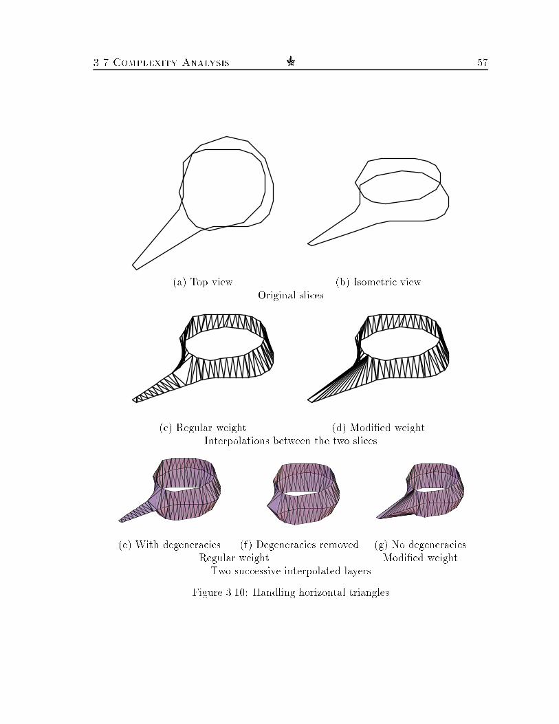
3.7 Complexity Analysis g 57(a) Top view (b) Isometric viewOriginal slices

(c) Regular weight (d) Modi�ed weightInterpolations between the two slices(e) With degeneracies (f) Degeneracies removed (g) No degeneraciesRegular weight Modi�ed weightTwo successive interpolated layersFigure 3.10: Handling horizontal triangles

58 Piecewise-Linear Interpolation between Polygonal SlicesComputing the contour nesting hierarchy in each slice and orienting the contoursin the correct directions takes O(k log k) time. This is performed by invoking a simpleline-sweep procedure.As in the gap-�lling problem (Chapter 2), the voting step, if it uses a hash table,can be executed with expected O(n) running time (assuming a reasonable choice ofthe proximity parameter "). Collecting the matches from the voting results and tilingthe matching contour portions require also O(n) time.Finding the remaining clefts can be done in O(n+ �) time. Finding their nestinghierarchy would take O((n + �) log(n+ �)) time, which is not desirable. Instead, weconsider only the original data points and the points of contour overlap, thus reducingthe time needed for this step to only O((k + �) log(k + �)). Finding the Euclideanminimumspanning trees for each cleft and its immediate children in the hierarchy canbe performed, using a naive brute-force technique (which works very well in practice),in overall O(�h2) time. The triangulation of each cleft is done in time cubic in its size,so this step requires a total of O(�h3) time, which is, theoretically, and in complexsituations also pragmatically, the most expensive part of our algorithm.To conclude, the entire algorithm runs on practical instances in average O((k +�) log(k + �) + n+ �h3) time.The following section describes our rather comprehensive experimentation withthe algorithm. In all cases that we tried, the running time was indeed small, andgenerally matched the bound given above.3.8 Experimental ResultsWe have implemented the whole algorithm in C on a Digital DECstation 5000/240, ona Sun SparcStation II, and on SGI Indigo and Indy workstations. The implementationtook about three man months, and the software consisted of about 5,000 lines of code.We have experimented with the algorithm on several data �les obtained by CT or MRIscanners, and obtained very good results in practically all cases. The input usuallyconsisted of about �fty to one hundred cross-sections, from 0.5 mm to 2.0 mm apart.The tuning of the parameters (discretization length and size of neighborhood in thegeometric hashing) was very robust, and large variation of these parameters producednearly identical results. We usually used 1.0 mm as the discretization parameter, and3.0 mm for the voting threshold (for human organs whose global size was between 5to 20 cm in all dimensions). For the voting step (see Section 3.5.2) we set M (halfof the width of the peak) to 7. We allowed up to two successive point mismatchesalong a match. A point-to-point match contributed the amount of 1=(d+ 0:1) to thematch score, where d was the horizontal distance between the two points (as de�nedin Section 3.3). We considered only match candidates which received 4 votes or more

3.8 Experimental Results g 59Figure 3.11: A synthetic example

Figure 3.12: A synthetic branching exampleand whose scores were above 15:0. (Our discretization was su�ciently dense so thatthis choice still captured all contour overlaps.) The objective function F for thecleft-triangulation was taken to be 0:85A+0:05P +0:10R, where A is the area of thetriangle, P is its perimeter, and R is the ratio between the largest and the smallestof its three edges. All these parameters were user de�ned, but modifying them didnot achieve any better results. (Recall that another possible �ne-tuning of F is toarti�cially increase the weight of horizontal triangles.)Here are some speci�c examples of the performance of the algorithm:Figure 3.11 shows a simple case, similar to the �rst problematic example of Bois-sonnat [Bo1]. Each slice in this example contains exactly one contour. The tiledmatch appears in white, whereas the triangulated cleft appears in black.Figure 3.12 shows a synthetic branching example, where the lower slice containstwo contours, whereas the upper slice contains only one contour. Two long matcheswere found and tiled by the white triangles. The remaining cleft appears in betweenthe two matches, and its triangulation appears in black. The two voting tables whichcorrespond to the matches are shown in Figure 3.13. The solid curves represent thenumber of votes (as functions of the shift); they are superimposed by the dotted

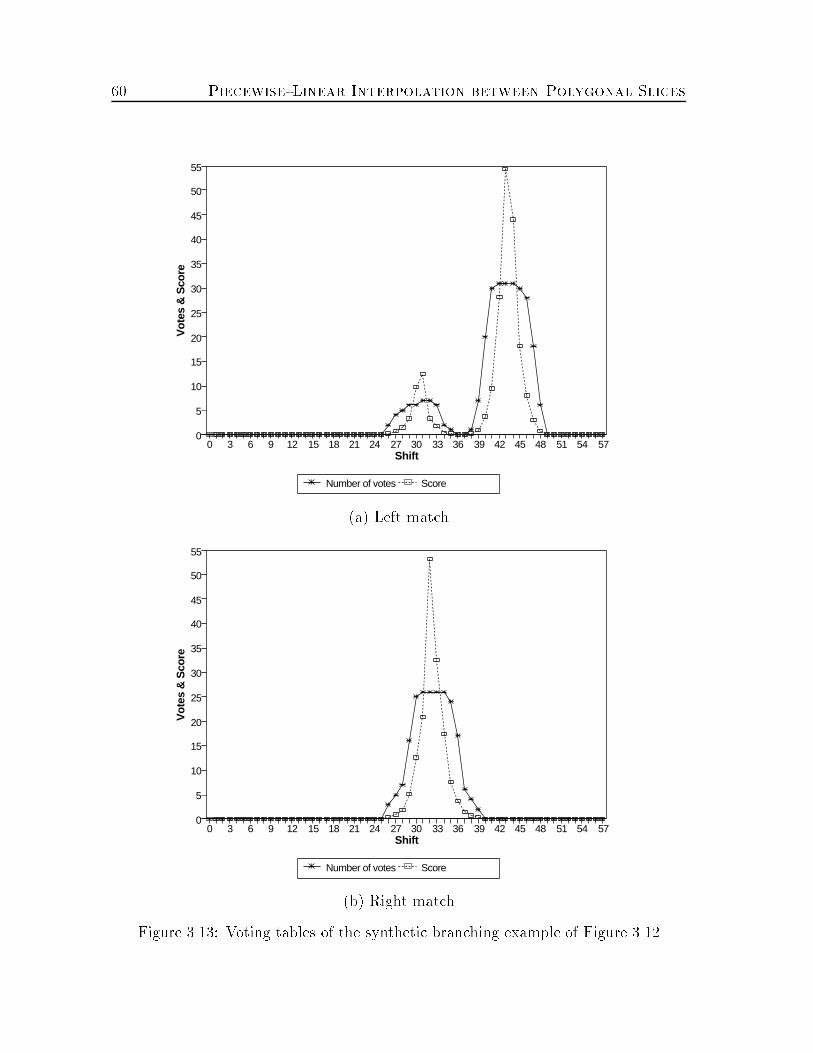
60 Piecewise-Linear Interpolation between Polygonal SlicesNumber of votes Score

0 3 6 9 12 15 18 21 24 27 30 33 36 39 42 45 48 51 54 57Shift

0

5

10

15

20

25

30

35

40

45

50

55V

otes

& S

core

(a) Left matchNumber of votes Score

0 3 6 9 12 15 18 21 24 27 30 33 36 39 42 45 48 51 54 57Shift

0

5

10

15

20

25

30

35

40

45

50

55

Vot

es &

Sco

re

(b) Right matchFigure 3.13: Voting tables of the synthetic branching example of Figure 3.12

3.8 Experimental Results g 61curves, which represent (in a di�erent scale) the score of each shift.Figure 3.14 shows a more complicated synthetic example, where the lower slicecontains one contour, and the upper slice contains three contours. Figure 3.14(a)shows a top view of this situation, whereas Figure 3.14(b) shows an isometric viewof it. Figure 3.14(c) shows the surface reconstruction. The tiling of the single matchappears in white. The remaining cleft consists of one cycle which encloses two othercycles. Two bridge constructions compose the three polygons into a single one, andits triangulation appears in black.The next several �gures show the typical performance of our algorithm, as ob-served from its execution on a series of cross-sections of a human jaw bone.Figure 3.15 shows the reconstructed surface between two slices. The tiles of thematches appear in white, and the triangulations of the two remaining clefts appearin black.Figure 3.16 presents a considerably more complicated situation, where the recon-struction turns out to be `intuitively correct'. Figure 3.16(a) shows that the lowerslice contains a contour with two hole contours, and the upper slice contains onlyone contour, which mostly lies above the \material" region of the lower slice. Thesurface reconstruction is shown in Figure 3.16(b). The three match tiles appear inwhite, and the cleft triangulations appear in black. The reader may verify that thetwo \non-material pillars" represented by the two hole contours in the lower slicewere connected to the unbounded \non-material" region in the upper slice.Figure 3.17 shows another multiple branching case which was resolved adequately.Besides the obvious contour matches, Figure 3.17(a) shows that the lower slice con-tains a single contour, which is split into four contours in the upper slice. Fig-ure 3.17(b) shows the reconstruction. The match tiles appear in white, whereas thecleft triangulations appear in black.Figure 3.18 presents a composite case. Figure 3.18(a) shows the two slices. Notethat the lower slice contains contours nested in three levels, that is, a \material"enclosed in a \non-material", which is in turn enclosed by \material" again. Fig-ure 3.18(b) shows the reconstruction. The match tiles appear in white, whereas thecleft triangulations appear in black. This interesting branching case consists of a holecontour (\non-material" region) in the lower slice, which encloses a \material" con-tour. These are transformed into one hole contour in the upper slice, which `bypasses'the inner \material" of the lower slice. The reader may verify again the intuitive cor-rectness of the reconstruction, which connects the inner \material" in the lower slicewith the outer (and only) \material" in the upper slice.The reconstruction of the whole jaw bone, whose input consisted of 96 slices, isshown in Figure 3.19. The result was a valid polyhedral description, which containedabout 60,000 triangles. The reconstructed jaw contained 209 3-D cavities (fully en-

62 Piecewise-Linear Interpolation between Polygonal Slices(a)

(b) Before reconstruction(c) After reconstructionFigure 3.14: A synthetic complicated example

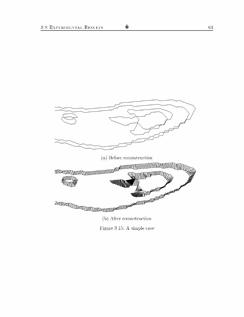
3.8 Experimental Results g 63

(a) Before reconstruction(b) After reconstructionFigure 3.15: A simple case

64 Piecewise-Linear Interpolation between Polygonal Slices

(a) Before reconstruction(b) After reconstructionFigure 3.16: A complicated branching case

3.8 Experimental Results g 65

(a) Before reconstruction(b) After reconstructionFigure 3.17: A multiple branching case

66 Piecewise-Linear Interpolation between Polygonal Slices

(a) Before reconstruction(b) After reconstructionFigure 3.18: A composite case

3.8 Experimental Results g 67

Figure 3.19: A fully reconstructed human jaw bone

68 Piecewise-Linear Interpolation between Polygonal Slices

Figure 3.20: Fully reconstructed human lungsclosed in the outer 3-D reconstructed boundary), each one described by a fully valid`anti-polyhedron', that is, a polyhedron whose boundary is oriented such that the`inside' of it is the unbounded space.The boundaries of other organs were also reconstructed successfully. An exampleof the reconstruction of a pair of lungs is shown in Figure 3.20. The input dataconsisted of 34 slices, and the reconstructed object contained about 8,400 triangles.The internal geometries of slices of the lungs were fairly complex. Figure 3.21shows the reconstruction between such a pair of slices. Figure 3.21(a) shows theoriginal slices, and the reconstruction is shown in Figure 3.21(b). The match tilesappear in white, whereas the cleft triangulations appear in grey. Figures 3.21(c,d)are closeups of the right cleft, in isometric and top views, respectively. The last two

3.8 Experimental Results g 69(a) Before reconstruction(b) After reconstruction

(c) Isometric view (d) Top viewCloseup of the right cleftFigure 3.21: A case with complex geometries

70 Piecewise-Linear Interpolation between Polygonal Slices�gures were rotated around the z-axis for a better view of the reconstruction.We have also reconstructed an amacrine cell of the retina (taken from an eyeof a Macaque monkey). The data contained 293 slices, obtained by an electronmicroscope. The 723 contours, which were made of 8,578 edges, were extremelydetailed. Figure 3.22 shows the full reconstruction of the cell, which consisted ofabout 24,000 triangles.Our experimentations were mostly performed on medical imaging data. However,as we mentioned in the introduction (Section 3.1), the reconstruction problem hasother applications as well. One such application is the reconstruction of a terrainfrom elevation contour data in topographic maps. This application is much simpler,because of the xy-monotonicity of terrains. For example, contours cannot overlap inthis case (although they can be nested).Figure 3.23 shows the reconstruction of a terrain in the Zikhron-Ya'akov area inIsrael. Figures 3.23(a,b) show the elevation contours (a top view and an isometricview). The data contained seventeen levels which are 10 meters apart, starting from20 and ending at 180 meters above see level. These levels consisted of 111 contoursmade of 5,329 edges. Figures 3.23(c,d) show the full reconstruction of the terrain(again, a top view and an isometric view).Table 3.1 summarizes the performance of our implementation on all the examplesdescribed above. All the time measurements were taken on a Digital DECstation5000/240 and on an SGI Indigo workstation. (Our SGI Indigo seems to be fasterthan our DECstation 5000/240 by a factor of roughly 3.) We note that in medicaldata, at least the data with which we experimented, successive slices tend to di�era lot in their geometries. Therefore, many clefts are created and their (relativelytime-consuming) triangulations a�ect the total running time of the algorithm. Thiswas not the case with the problem we investigated in the previous chapter, namelythe detection and repair of gaps in the boundary of a polyhedron. There we had holesinstead of clefts, whose size turned out to be bounded on the average by a constant,which was a function of the parameters given to the algorithm.3.9 ConclusionWe have proposed in this chapter an algorithm for solving the practical problem ofpolyhedral interpolation between parallel polygonal slices. This problem has manymedical and geographic applications, and also appears to be a fairly basic and inter-esting problem in computer graphics and solid modeling.We have combined several techniques to obtain our solution. First, we used a par-tial curve matching technique based on geometric hashing, adapted from computervision, for identifying matching contour portions. Then, we tiled the matching por-

3.9 Conclusion g 71

Figure 3.22: An amacrine cell of the retina

72 Piecewise-Linear Interpolation between Polygonal Slices

(a) (b)(c) (d)Figure 3.23: A topographic terrain

3.9 Conclusion g 73VerticesContours After DiscretizationModel Slices Layers Total Per Slice Original Total Per ContourSynthetic 2 1 3 1.5 50 143 47.7Jaw Bone 96 95 417 4.3 12,702 17,646 42.3Lungs 34 33 88 2.6 3,121 4,232 48.1Retina Cell 293 292 723 2.5 8,578 11,945 16.5Topog. Map 17 16 111 6.5 5,360 5,584 50.3Matches Clefts Cleft PointsModel Total Per Layer Total Per Layer Total Per CleftSynthetic 2 2.0 1 1.0 28 28.0Jaw Bone 330 3.5 275 2.9 3,592 13.1Lungs 89 2.7 39 1.2 821 21.1Retina Cell 701 2.4 105 0.4 1,041 9.9Topog. Map 69 4.3 131 8.2 3,015 23.0Time (Seconds)All Layers PerModel Machine Stitching Triangulation Total LayerSynthetic DEC 5000/240 0.07 0.13 0.20 0.20SGI Indigo 0.03 0.04 0.07 0.07Jaw Bone DEC 5000/240 12.50 37.12 49.62 0.52Lungs SGI Indigo 2.15 1.97 4.12 0.13Retina Cell SGI Indigo 14.60 3.38 17.98 0.06Topog. Map SGI Indigo 2.74 11.91 14.65 0.92Table 3.1: Performance of the reconstruction algorithm

74 Piecewise-Linear Interpolation between Polygonal Slicestions using a simple `merge-like' advancing rule. Finally, we identi�ed the remainingclefts and employed a minimum spanning-tree technique for simplifying the clefts,followed by a minimum-area triangulation of 3-D polygons in order to �ll them. Wealso used a line-sweep procedure to identify the hierarchy of contour nesting in a slice.Our method produces a relatively smooth boundary, due to the contour discretiza-tion. In situations where the addition of new vertices is not desired, e.g. due to dataexplosion, our system uses the discretization only for the matching step, but the tilingitself and the following minimum-area triangulation are performed on the contourscontaining only the original points.We feel that our technique reconstructed the boundary of various organs in anintuitively appealing manner; one might say that our algorithm demonstrated some`understanding' of the underlying problem. The results were more than adequateeven in extreme cases of tiling between two seemingly totally di�erent slices.We plan to continue the experimentation with our algorithm, to test its perfor-mance limits and see if there are data instances on which the algorithm might notperform well, thus requiring further calibrations and enhancements (in view of ourexperimentation so far, we doubt that anything really problematic will arise).

Chapter 4Partial Surface and VolumeMatching in Three Dimensions4.1 IntroductionThe problem of �nding a full or a partial match between three-dimensional objectsattracted considerable attention in the literature during the past decade. The mainmotivation for this problem comes from the object recognition problem in computervision (see Chapter 1). Partial matching, due to object occlusion or because a sensorusually cannot scan all sides of the object, is acknowledged by many researchers asa major problem in object recognition (cf. [BJ1, p. 137]). Another signi�cant moti-vation for the surface matching problem is docking of proteins in molecular biology,where a geometric �t between parts of the boundaries of two molecules (i.e., a partialsurface matching) is sought, requiring also that the molecules do not overlap nearthe matched boundaries. Important applications of molecule docking are the recogni-tion and binding of receptors and ligands, and synthetic drug design. Partial volumematching can also aid in the detection of structural motifs in proteins, thus adding tothe understanding in their role and functionality [AM2]. Yet another motivation is thecombination of several snapshots of the same object, taken from di�erent view points,in order to obtain a description of a bigger portion of its boundary. This has obviousindustrial, civil, and military applications (e.g. the decoding of aerial photographs),and is closely related to the �eld of active vision, which is currently an intensive topicof research (cf. [BY]). Another important motivation is the registration of medicalimages obtained from the same or di�erent modalities. In many cases, more than oneimaging technique is used in clinical diagnosis, therapy planning, and in evaluationof therapy. Integrating the complementary information obtained from several studiesof the same patient can be a valuable tool in the treatment of the patient. Notethat, in most of these applications, we are only seeking a partial match between the75

76 Partial Surface and Volume Matching in Three Dimensionsimage and the model objects, or between two protein molecules, or between di�erentviews of the same object. Medical image matching, however, usually involves a globalmatch (registration) of a whole organ.4.1.1 Previous WorkWe �rst brie y review the fairly extensive literature on the problem of surface or vol-ume matching, studied mainly in the context of computer vision and pattern recogni-tion. Some works (e.g. [BH]) depend on the ability to match signi�cant features of theobjects, like knobs and holes, whose existence is not usually guaranteed. Other meth-ods, which do not rely on the existence of a certain type of features, are pose-clustering[St], alignment [HU1, HU2], and, of course, geometric hashing. A comparison betweenthese techniques is found in [Wo1]. Comprehensive surveys on partial surface match-ing techniques in computer vision are found in [BJ1, CD]. To quote from the recentpaper [BM], \Relatively little work has been published in the area of registration(pose estimation, alignment, motion estimation) of 3-D free-form shapes. Most of theexisting literature addressing global shape matching or registration have addressedlimited classes of shapes, namely, 1) polyhedral models, 2) piecewise-(super)quadraticmodels, and 3) point sets with known correspondence."Many other works have addressed the problem; see [Po1, Po2, Be1, Be2, Fi1,Ho2, Ho3, HH, Br1, FHKL, SE, BA, Fa, FH, GL, AHB, Sz, Ta2, Ta3, KJR, BM,HNR, HKR]. Most of these works have various limitations, some of which are quitesevere. They either restrict the shape of the matched objects (e.g., require themto be polyhedra, or to have large planar portions, or study only planar objects), orassume that there is no occlusion (so a full matching between the objects is sought),or handle only restricted motions, involving fewer than six degrees of freedom. Themethods that do not have these restrictions (e.g., those of [Fa, FH, Ho3, BM]) haveother disadvantages. For example, some of them are sensitive to statistical outliers,which have to be removed in a preprocessing step. Other methods might converge toa motion that yields only a local extremum of their `scoring function', etc.Potmesil [Po1, Po2] de�nes surface matching as \�nding a spatial registration oftwo surface descriptions that maximizes their shape similarities". Potmesil describesa heuristic algorithm, which searches for the best matching transformation, where thecandidate transformations are evaluated at some selected points, e.g. surface controlpoints and points of maximumcurvature. Besl [Be1, Be2] provides a similar de�nitionof the registration problem, and gives some metrics for measuring matches betweencurves and surfaces.Fisher [Fi1] suggests a set of heuristics for obtaining a registration between twoobjects by using their 2-dimensional boundaries (the so-called silhouettes). Horn [Ho2]and Brou [Br1] develop the extended Gaussian image method, which uses a surface

4.1 Introduction g 77normal histogram for matching convex (and some restricted nonconvex) shapes.Fang et al. [FHKL] and Stockman and Esteva [SE] solve a constrained registrationproblem, where the aligned objects are polyhedra, and where only translations androtations in the xy-plane are allowed. They extract some edge- and point-features,and accumulate a three-dimensional histogram of possible matches, in which clustersare assumed to indicate possible matches. Boyter and Aggarwal [BA] also allow onlyone degree of rotational freedom, but use a di�erent approach.Faugeras [Fa] and Faugeras and Hebert [FH] use quaternions for converting thethree-dimensional rotation problem into a four-dimensional minimumeigenvalue prob-lem, while the translation is found by using a standard least-squares technique. Thematching is performed on parameter vectors, which are associated with every geomet-ric primitive, such as planes. Horn [Ho3] suggests instead to look for the maximumeigenvalue. (Although we do not use quaternions, we present a similar idea for avariant of our approach; see Section 4.8.)Alternatively, Golub and van Loan [GL] and Arun, Huang, and Blostein [AHB]use the singular value decomposition. The main de�ciency of their method is relyingon the existence of signi�cantly large planar regions in the objects.Szeliski [Sz] uses a standard steepest descent heuristic for generating a series ofrotations of one object relative to the other. His goal is to minimize the sum ofweighted di�erences (along the z-axis only) between points of the two objects. Theapplication is the computation of a motion estimation of an observer, which scansthe same object from two view points. Horn and Harris [HH] present a similar (butfaster) technique, which, however, seems to produce satisfactory results only whenthe motion is relatively small.Taubin [Ta2, Ta3] approximates data point sets with algebraic surfaces up tothe tenth degree, with an application to global position estimation (that is, withoutocclusion). Kamgar-Parsi, Jones, and Rosenfeld [KJR] present a \2.5-dimensional"registration method, which is actually a matching problem in 2-space.Besl and McKay [BM] register three-dimensional shapes (of various types) byusing the so-called ICP (iterative closest point) algorithm. This algorithm iterativelyinvokes a procedure, which �nds the closest member of a point set to another givenpoint. The algorithm converges very quickly to a local minimum of a mean-squaredistance metric, so it is applied from several starting rotations, hoping not to missthe global minimum.Finally, Huttenlocher, Noh, and Rucklidge [HNR] track moving objects in a seriesof two-dimensional raster images, by using the minimum Hausdor� distance undertranslations between two sets of points. They actually match portions of the twoimages. Their method assumes that the orientations of occurrences of the sameobject in successive images di�er by only a relatively small amount. This work thus

78 Partial Surface and Volume Matching in Three Dimensionsconsiders only translations, and explicitly assumes that the rotation component ofthe rigid motion of the object is relatively small. In a companion work, Huttenlocher,Klanderman, and Rucklidge [HKR] present an e�cient algorithm for computing theminimum Hausdor� distance between images, allowing translations and rotations.None of the methods listed so far is based on geometric hashing. Approaches thatdo employ geometric hashing for surface and volume matching were developed mainlyin the context of molecular biology applications, which we now proceed to review. Themain problem in generalizing the geometric hashing technique to partial matchingbetween surfaces (as opposed to curves) is that, in its original application to partialcurve matching, it depends on the linear order of the given curves, which is neededfor computing the relative `shift' between matching portions of the curves. There aresigni�cant technical problems in naive attempts to extend this technique to (partial)matching between 2-dimensional surfaces or 3-dimensional volumes. Nevertheless,there have been several earlier attempts at such an extension, as will be discussedbelow.The surface and volume matching problems that arise in molecular biology fallinto two main kinds. One typical problem is to �nd a `docking' of two molecules(or subunits of the same molecule). Here we seek a rigid motion of one moleculerelative to the other, which creates a good geometric �t between large portions of themolecule boundaries, so that the molecules themselves remain disjoint; that is, we seeksurface matching and volume complementarity. (In practice, docking of moleculesmay depend also on a good chemical/electrical �t between the atoms participatingin the docking. The purely geometric statement of the problem is thus only anapproximation of the problem, but it is appropriate in many cases.) Another problemis to detect similar 3-dimensional structural motifs in macromolecules. Here we alsoseek a rigid motion that will create a good �t between large portions of the moleculesurfaces, but we want their volumes to overlap near this �t.The standard representation of a molecule is just a list of its atoms and theirspatial positions. Consequently, a major di�culty in studying molecule docking andstructural motifs is in the de�nition and computation of the molecule boundary.Richards [Ri] de�nes the solvent-accessible surface of a macromolecule to consist ofall the atom `boundaries' reachable by the surface of a `water' ball (of diameter 1.4 �A),which moves continuously in space and does not intersect any atom (in this approach,atoms are represented as balls of various radii). This de�nition of the boundary sur-face of a macromolecule is used in many later works, e.g. [Co3, FNNW]. Connolly[Co1, Co2] proposes the MS algorithm for computing such a molecule surface. An-other algorithm for this problem, exploiting computational geometry techniques, wasrecently proposed (and implemented) by Halperin and Overmars [HO].First attempts to solve the molecule docking problem, which are based on energyminimization (references 1{6 of [KSEF]), were only partially successful. Geometricapproaches (references 7{16 of [KSEF], including [Co3]) were much more successful,

4.1 Introduction g 79but (at least the earlier ones) were not reliable enough, and su�ered from unacceptedlylong computation time [KSEF].Kuntz et al. [KBOL] transform the structures of the ligand and of the receptor oftwo proteins into a graph, in which they search for 4-cliques. Each detected cliqueis mapped into a 3-dimensional transformation, and checked for possible penetrationof the ligand into the receptor, in which case it is rejected. Similarly, Kuhl, Crippen,and Friesen [KCF] construct a graph, in which they search for the maximum clique.Although this problem is NP-Complete in general, they claim to obtain a randomizedalgorithm whose practical running time is O((nm)2:8), where n andm are the numbersof atoms in the ligand and the receptor, respectively. As remarked above, thesegeometric approaches, as well as the other approaches described below, are based onthe assumption that the sites of chemical reaction do not change their geometriessigni�cantly during the reaction. This assumption holds in many cases; however,exceptions to it are known and are not that rare (e.g., the complex trypsin-trypsininhibitor [KSEF]).Other geometric methods [JK, KSEF] perform a brute-force search over all thediscretized 3-dimensional rotations, while using a secondary method for identifyingthe appropriate translation. The paper [KSEF] uses a correlation function for de-termining the translation; this function is computed e�ciently by using the discreteFourier transform.Traditional methods for detecting structural motifs in proteins usually employalgorithms for string comparison, where the strings represent the primary structures(amino acid sequences) of the proteins. A survey of these methods, most of whichare based on dynamic programming, is found in [SK]. Enhanced methods [RK, AM1,MARW] also consider prede�ned motifs (such as the so-called �-helixes and �-sheets)in the secondary structures of the molecules.A major contribution to the problems of detecting structural motifs and of mole-cule docking was achieved by application of techniques based on geometric hash-ing. This method facilitates the handling of a priori totally unknown 3-dimensionalstructures. In this application, the method proceeds by assigning footprints to themolecule atoms, then by matching the footprints and by voting for the relative trans-formation (rigid motion) of one molecule relative to the other, assuming that thecorrect transformation will receive signi�cantly more votes than all the others (inthe spirit described in Section 1.3). For the motif detection, Nussinov and Wolfson[NW] de�ne the footprint of each atom as its coordinates in systems de�ned by anynon-colinear triple of atoms (thus each atom has O(n3) footprints, where n is thenumber of atoms in the molecule). Similar ideas are presented in [FBNW, FNW].Fischer et al. [FNNW] take a similar approach for the molecule docking problem. Inone variant, each pair of atoms de�nes a basis (whose length is the distance betweenthe two atoms), and the footprint of every atom is de�ned as the distances from theatom to the endpoints of every basis, coupled with the length of the basis (thus each

80 Partial Surface and Volume Matching in Three Dimensionsatom has O(n2) footprints). In another variant, the angles between the normal tothe surface (at the candidate atom) and the normals at the endpoints of the basis,as well as a knob/hole label (obtained by Connolly's MS algorithm) of the atom, arealso considered. In all cases, the footprints are stored in a hash table, as in any otherapplication of geometric hashing, which allows to retrieve entries with some toler-ance. Here this is needed not just because of the noisy footprints, but also becauseof the conformational changes that might occur in the molecule structures during thereaction between them.Finally, we brie y describe the topic of medical image matching, which has at-tracted a lot of attention in the medical literature. The problem arises when com-plementary information about some organ is obtained by several imaging techniques,such as CT (Computed Tomography), DSA (Digital Subtraction Angiography), EEG(Electroencephalography), MEG (Magnetoencephalography), MRI (Magnetic Reso-nance Imaging), MRS (Magnetic Resonance Spectroscopy), PET (Positron Emis-sion Tomography), SCECoG (Subchronic Electrocorticography), SEEG (Stereoen-cephalography), SPECT (Single Photon Emission Computed Tomography), and oth-ers. The goal is to match (register) the various models of the same organ obtainedby these methods, in order to obtain an improved and more accurate model. Sucha registration is needed because the orientations of the organ usually di�er from onemodel to another.Many methods, which are similar to the methods for object recognition, were pro-posed for the solution of this organ registration problem. These include, amongmany others, approximated least-squares �t between a small number of markers(e.g., [HBGJ, HHLR]), singular value decomposition for matching point pairs (e.g.,[EMCP, HHCG]), high order polynomials for a least-squares �t [SFSH, KDVE], \thin-plate spline" for registering intrinsic landmarks [Bo3] or extrinsic markers [Bo2], para-metric correspondence (e.g., [CPCC, PCSW]), chamfer maps (e.g., [BTBW, Bo4,Bo5, HHH, JHR, JRH, EMV, EMPV]), partial contour matching [Mo], moments andprincipal axes matching (e.g., [GGC, GFC, KGCR, TUHW, ABKC]), and correlationfunctions (e.g., [VGLP, CCMM, BK, MFP, JMHB, CPDE, CPE]). Brown [Br2] givesan exhaustive overview of image registration techniques. Another detailed review ofprevious work, with classi�cation of the matching techniques, is given by van derElsen, Pol, and Viergever [EPV]. They classify the di�erent methods for register-ing medical images according to their dimensionality, image properties (intrinsic orextrinsic), domain of transformation (global or local), \elasticity" of transformation(rigid, a�ne, projective, etc.), tightness (the relation assumed between the matchedimages), and the method of parameter determination (directly or by searching).

4.1 Introduction g 814.1.2 Our ApproachWe propose a new approach to the matching problem, and present several of itsapplications in the domains mentioned above. Our algorithm accepts any pair ofpoint sets in 3-space, describing either the volumes or the boundary surfaces of twoobjects, and attempts to �nd the best rotation and translation of one object relativeto the other, so that:(i) if the given sets represent object boundaries, then there should be a good geo-metric �t between large portions of these boundaries;(ii) if the given sets represent object volumes, then there should be a large �tbetween the boundaries of the objects, so that their volumes either overlap orremain disjoint near the �t.In the �rst case, our algorithm solves the (partial) surface matching problem. Inthe second case, it solves the (partial) volume matching problem, either with volumeoverlap or with volume complementarity.Here is a brief overview of our algorithm. First, we associate with each point ofthe two sets a footprint. As usual, this value should be invariant under rotations andtranslations, and should be `descriptive', in the sense that points of the two sets whoselocal neighborhoods admit a good match should have similar footprints, whereaspoints whose local neighborhoods do not �t well together should have signi�cantlydi�ering footprints. Next, we de�ne a scoring function that measures the `goodness'of a speci�c rotation (of one set relative to the other), and is invariant of the relativetranslation. In an ideal setting, this function has a global maximum at the correctrotation, and does not have any other signi�cant local maxima. This enables usto advance from any rotation towards the correct rotation, by invoking the scoringfunction iteratively, and by deciding locally in which direction to advance. Finally,we compute the best translation associated with the �nal rotation. The variousapplications of our algorithm mainly di�er in the de�nition and computation of thefootprints. Di�erent footprints are needed for the surface matching problem and forthe two types of the volume matching problem. In addition, the manner in which thesets representing the objects were obtained can also in uence the choice of footprints.Needless to say, the choice of footprints is a crucial factor that in uences the successof our method.In comparing our algorithm to previous works on surface matching, as mentionedabove, we can say that our algorithm appears to be robust even in the presence ofconsiderable noise in the input data (or of excess data that is irrelevant for the partialmatch that we seek). Therefore, we do not need to remove, in a preprocessing step,data that represent statistical outliers.

82 Partial Surface and Volume Matching in Three DimensionsOur algorithm does not depend on any correspondence between the two sets ofinput data points. It does not attempt to extract any predetermined features of theobjects described by the data sets, thus it does not depend on the existence of anysuch features. It does not rely on surface derivatives (although the footprint we chosefor the car models|see Section 4.9|can be regarded as a weak form of a derivative).In practice, our algorithm is very easy to implement, and it runs in a practical timewith practical inputs, which compares favorably with reported performance of earlieralgorithms. It produced very accurate results in all the cases that we tested and arereported here. The generalization of our algorithm to higher dimensions should bestraightforward.The only detail preventing the algorithm from being a fully automated tool formatching any two point sets is the need to assign `descriptive' footprints to all thepoints. This seems to require customized treatment for each class of applications.We do not regard this as a de�ciency of our algorithm, but rather as an advantageof it: Whereas most of the previous registration algorithms actually regard the 3-dimensional coordinates of each point as its footprint, we achieve greater versatilityof the matching process through the additional information hidden in any speci�csystem of footprints. We emphasize again that the choice of footprints does greatlyin uence the success of the subsequent matching procedure.The main di�erences between the application of our algorithm to molecule dockingand similar works on this problem based on geometric hashing (e.g., [FNNW, Fi2])are the following:1. We use all the atoms on the molecule boundaries instead of using only \points(atoms) of interest". (For example, the technique of [Fi2] uses only the `back-bone' C-atoms of the polypeptide chain of a protein.)2. We generate a footprint for each individual atom in each molecule, and not forpairs or triples of atoms, as do the earlier methods. Consequently, we havemuch fewer footprints, and thus also much fewer voting entities.3. However, the other methods vote directly for a rotation, whereas we vote for animaginary translation at any �xed orientation. Thus, the other methods haveonly one voting process, whereas we generate a series of rotations and vote ateach one of them separately.We have implemented and experimented with our algorithm on several types ofinput. In this chapter, we describe the performance of our algorithm on several exam-ples taken from industrial applications (one involving volume matching between twoobjects given in CAD �les, and one involving partial surface matching between twoimages, obtained by range-scanning the same object from two di�erent view points),from molecular biology (involving the solution of the molecule docking problem for

4.2 Rationale: The 2-Dimensional Case 83two pairs of hemoglobin subunits, the identi�cation of common structural motifs inone pair of hemoglobin subunits, and the docking of another receptor to a ligand),and from medical imaging (involving the registration of two MRI scans of the samefunctional brain `phantom'). In almost all cases, the algorithm worked well and com-puted correctly the expected matches, in spite of the large amount of noise presentin the data, and of the fact that in most applications only a partial match did exist.Our technique was most successful in the industrial and medical applications,where the quality of the data allowed us to generate good footprints, and was moreproblematic (though still reasonably successful) in the molecular biology applications,where the footprints generated by the current version of our algorithm are of poorerquality, due to the nature of the input data. We feel that the di�culties that wefaced with molecule docking were not due to inherent limitations of the algorithm,but rather because of inadequate preprocessing of the data, namely not quite accuratecomputation of the boundary atoms of the molecules and, consequently, the produc-tion of poorer-quality footprints for them. We hope to improve upon this issue infuture versions of our software.This chapter is organized as follows. In Section 4.2 we describe the rationale forthe algorithm proposed in the following sections, by examining a 2-dimensional vari-ant of the problem. Section 4.3 presents an overview of the algorithm (more detailedthan the one given above). The later sections describe in detail the various phases ofthe algorithm: Section 4.4 describes the data acquisition phase, Section 4.5 describesthe scoring of a candidate rotation, Section 4.6 describes the heuristic of advanc-ing towards the `best' rotation (the one that has the highest score), and Section 4.7describes the determination of the translation associated with the best rotation. Sec-tion 4.8 describes an alternative statistical approach in 3 dimensions, which reducesthe problem, in favorable situations, to a 2-dimensional problem. Section 4.9 presentsthe experimental results mentioned above. We end in Section 4.10 with some con-cluding remarks.4.2 Rationale: The 2-Dimensional Case4.2.1 Structure of Voting TablesThe motivation for our algorithm arose from our experimentation with matchingsynthetic sets of points in 2 dimensions. The input consisted of a point set A inIR2, and of another point set B, obtained from A by rotating (by some angle �) andtranslating. The sets did not contain any noise, and the footprints of the points werechosen in an arti�cial way that ensured a nearly perfect match.Consider, for example, the set shown in Figure 4.1, hereafter referred to as thearrow A. As seen in the �gure, the points belong to a regular grid. Each point was

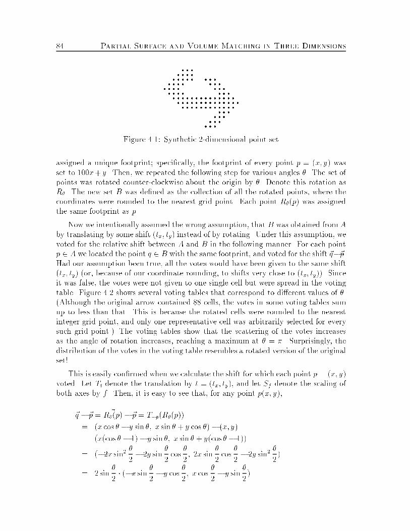
84 Partial Surface and Volume Matching in Three Dimensions� � �� � � �� � � � � � � �� � � � � � �� � � � � � �� � � � � � �� � � � � � � � � � � � � �� � � � � � � � � � � � � �� � � � � � � � � � � �� � �� � �� � �� � �Figure 4.1: Synthetic 2-dimensional point setassigned a unique footprint; speci�cally, the footprint of every point p = (x; y) wasset to 100x+ y. Then, we repeated the following step for various angles �. The set ofpoints was rotated counter-clockwise about the origin by �. Denote this rotation asR�. The new set B was de�ned as the collection of all the rotated points, where thecoordinates were rounded to the nearest grid point. Each point R�(p) was assignedthe same footprint as p.Now we intentionally assumed the wrong assumption, that B was obtained fromAby translating by some shift (tx; ty) instead of by rotating. Under this assumption, wevoted for the relative shift between A and B in the following manner. For each pointp 2 A we located the point q 2 B with the same footprint, and voted for the shift ~q�~p.Had our assumption been true, all the votes would have been given to the same shift(tx; ty) (or, because of our coordinate rounding, to shifts very close to (tx; ty)). Sinceit was false, the votes were not given to one single cell but were spread in the votingtable. Figure 4.2 shows several voting tables that correspond to di�erent values of �.(Although the original arrow contained 88 cells, the votes in some voting tables sumup to less than that. This is because the rotated cells were rounded to the nearestinteger grid point, and only one representative cell was arbitrarily selected for everysuch grid point.) The voting tables show that the scattering of the votes increasesas the angle of rotation increases, reaching a maximum at � = �. Surprisingly, thedistribution of the votes in the voting table resembles a rotated version of the originalset!This is easily con�rmed when we calculate the shift for which each point p = (x; y)voted. Let Tt denote the translation by t = (tx; ty), and let Sf denote the scaling ofboth axes by f . Then, it is easy to see that, for any point p(x; y),~q � ~p = ~R�(p)� ~p = T�p(R�(p))= (x cos � � y sin �; x sin � + y cos �)� (x; y)= (x(cos � � 1)� y sin �; x sin � + y(cos � � 1))= (�2x sin2 �2 � 2y sin �2 cos �2 ; 2x sin �2 cos �2 � 2y sin2 �2)= 2 sin �2 � (�x sin �2 � y cos �2 ; x cos �2 � y sin �2)

4.2 Rationale: The 2-Dimensional Case 8515-25 88(a) � = 0 13 14 15-22 4-23 8 25 6-24 11 18-25 6 10(b) � = �18 08 09 10 11 12 13 14-18 3 1 1-19 4 4 4 1-20 3 2 4 1 3 2-21 4 1 4 2 1-22 1 3 3-23 2 2 4-24 2 4 1 3 4-25 1 1 4 4 1-26 1 2(c) � = �601 02 03 04 05 06 07 08 09 10 11-14 1 1 1-15 1 1 1 1 1 1 1 1-16 1 1 1 1 1 1 1 1 1-17 1 1 1 2 1 1-18 1 1 2 1 1-19 1 1 1 1 1 1-20 1 1 1 1 1-21 1 1 1 2 1-22 1 1 1 1-23 1 1 1-24 1 1 1-25 1 1 1 2 1-26 1 1 1 1 2 1-27 1 1 1 1 1 1 1-28 1 1 1 1 2-29 1 1(d) � = �3-6 -5 -4 -3 -2 -1 00 01 02 03 04 05 06 07-14 1 1 1 1 1 1-15 1 1 1 1 1 1-16 1 1 1 1 1 1 1-17 1 1 1-18 1 1 1 1-19 1 1 1 1-20 1 1 1 1 1-21 1 1 1 1-22 1 1 1 1 1-23 1 1 1 1-24 1 1 1 1 1-25 1 1 1 1-26 1 1 1-27 1 1-28 1 1-29 1 1 1-30 1 1 1 1 1-31 1 1 1 1 1 1-32 1 1 1 1 1-33 1 1 1 1 1(e) � = �2.. .. .. .. .. .. .. .. -9 -8 -7 -6 -5 -4 -3 -2 -1 00 01 02 03 04 05 06 07 08 09 10 11 12 13 14 15-25 1 1 1-26-27 1 1 1-28-29 1 1 1-30-31 1 1 1-32-33 1 1 1 1 1 1 1 1 1 1 1 1-34-35 1 1 1 1 1 1 1 1 1 1 1 1 1 1-36-37 1 1 1 1 1 1 1 1 1 1 1 1 1 1-38-39 1 1 1 1 1 1 1-40-41 1 1 1 1 1 1 1-42-43 1 1 1 1 1 1 1-44-45 1 1 1 1 1 1 1 1-46-47 1 1 1 1-48-49 1 1 1(f) � = �04 05 06 07 08 09 10 11 12 13 14 15 16 17 18 19 20 21 22 23-33 1 1 1 1 1-34 1 1 1 1 1 1-35 1 1 1 1 1 1 1-36 1 1 1 1 1 1 1 1-37 1 1 1 1 1 1-38 1 1 1 1 1 1 1-39 1 1 1 1 1 1-40 1 1 1 1 1 1 1-41 1 1 1 1 1 1 1-42 1 1 1 1 1 1-43 1 1 1 1-44 1 1 1 1 1 1 1-45 1 1 1 1 1 1-46 1 1 1 1 1 1(g) � = 3�2 14 15 16 17 18 19 20-26 1 1-27 1 4 4 1-28 2 4 1 4 3-29 2 4 2 4-30 3 4 2 1-31 4 2 4 2 1 2-32 1 4 4 3 3 1-33 3 3 2-34 1(h) � = 11�6Figure 4.2: Voting tables corresponding to few values of �

86 Partial Surface and Volume Matching in Three Dimensions= 2 sin �2 � (x cos(�2 + �2)� y sin(�2 + �2); x sin(�2 + �2) + y cos(�2 + �2))= S2 sin �2 (R�2+ �2 (p)) :Hence, if the rotation of B relative to A is �, then each point p votes for the imaginaryshift ~q� ~p, which is obtained by �rst rotating p around the origin by �2 + �2, and thenby scaling it by 2 sin �2 . This means that the voting table actually shows the shape ofthe original set rotated by �2 + �2 and scaled by a factor of 2 sin �2 . For example, referto the case � = � shown in Figure 4.2(f). The voting table shows the original arrowA rotated by � and scaled by a factor of 2.This suggests the following technique for determining the goodness of a rotation! between A and B. We rotate A by !, and vote for the shift between R!(A) and B.The closer ! is to the correct rotation �, the more `compact' is the resulting votingtable. That is, the votes should appear to be clustered around some `accumulationpoint'.Note that the assumption that the rotation is about the origin is made for sim-plicity only and without any loss of generality. To see this, suppose that the rotationR� is about some point c, or, equivalently, R� is about the origin but is followed bya translation by t = (I �R�)(c). Then, the resulting voting table would look as if itwere associated with a rotation around the origin, with the only di�erence that it isshifted by t. Except for this, it remains unchanged.Recall that when the relative rotation between A and B is �, each point p 2 Acontributes one vote to the shift S2 sin �2 (R�2+ �2 (p)). Apart from round-o� errors, therotation R�2+ �2 does not in uence the density of the voting table. Thus, the onlyfactor that causes the votes not to be gathered at a single cell of the voting tableis the scaling e�ected by S2 sin �2 . Since the sine function sin �2 is continuous over thespace of orientations � 2 [0; 2�] and has a unique minimum (at 0) and a uniquemaximum (at �), we expect the voting table to be the most sparse when our `guess'! deviates from the real � by �, i.e. when j� � !j = �, to be the most dense when� = !, and to vary continuously and monotonically between these two extremes. Thissuggests that we use a scoring function that measures the sparseness of the votingtable, giving higher scores to more compact tables, and then apply a simple iterativebinary search step that varies the rotation in the direction that makes the table morecompact.4.2.2 Choosing a Scoring FunctionNext we need to de�ne a scoring function, in order to evaluate the voting tableassociated with any speci�c candidate rotation. This scoring function should varycontinuously and monotonically between a minimum at � + � (modulo 2�) and a

4.2 Rationale: The 2-Dimensional Case 87maximum at �. Intuitively, given two rotation angles, the scoring function shouldgive a higher score to the voting table which is denser and more concentrated.The �rst naive scoring function that we tried was simply the sum of squares of theentries in the voting table T . That is, we de�ned the score SC0(T ) = Pni=1M2i , wheren was the number of cells in T , and Mi was the number of votes given to the ithcell. The performance of this scoring function was very good in our experiments intwo dimensions, as well as in our experiments in three dimensions which involved fullmatching of data free from noise. It failed, however, in cases of partial matching, orwhen the data was noisy. We describe in detail in Section 4.5 the scoring function thatwe actually used in our experimentation, but, for the 2-dimensional case consideredhere, the scoring function SC0(T ) performed just as well. (We note that none of thesefunctions is perfect, since in practice they may also have local maxima. However,each such point is typically maximal within a rather small neighborhood, and thetechniques that we use for advancing towards the optimal orientation usually makesure that we do not get stuck at such a maximum.)4.2.3 Advancing Towards the OptimumIn two dimensions the process of advancing towards the angle with the highest scoreis fairly straightforward. We invoke a procedure similar to a variant of the parametricsearching of Megiddo [Me1] (or, rather, of binary searching; see [To]), in which wealways maintain a triple of angles, whose range contains the angle with the maximumscore. This range is shrunk in each step, by computing the score of some angle withinthis range, which, together with two of the previous angles, de�nes a new triplebounding a smaller range, which still contains the optimum angle.In more detail, we proceed as follows. First, we evaluate the scores of the rotationangles 0, 2�=3, and 4�=3. The triple (a0; a1; a2) of rotation angles is initialized sothat it is in counter-clockwise order and the angle with the highest score amongthese three angles is assigned to a1. The range de�ned by this triple has a0 as itsclockwise endpoint and a2 as its counter-clockwise endpoint. Denote the scores of thethree angles by (s0; s1; s2). Since the (ideal) scoring function has a unique maximum,at some angle a�, it is easily veri�ed that a� must lie in the range (a0; a1; a2). Wemaintain the invariant that s1 is always greater than s0 and s2, and iteratively performthe following procedure (all the angle di�erences are computed modulo 2�):1. If a2 � a0 < ", then put a� = a1 and return.2. If a1 � a0 > a2 � a1, then put a3 := (a0 + a1)=2 and set side to `left'; else puta3 := (a1 + a2)=2 and set side to `right'.3. Evaluate s3 (the score of a3).

88 Partial Surface and Volume Matching in Three Dimensions4. If side = `left', then do:(a) If s3 � s1, then put (a0; a1; a2) := (a0; a3; a1) and (s0; s1; s2) := (s0; s3; s1);(b) Else if s0 � s3 < s1, then put (a0; a1; a2) := (a3; a1; a2) and (s0; s1; s2) :=(s3; s1; s2);(c) Else (s3 < s0) halt the algorithm with an error (since this contradicts themonotonicity assumption).5. Else (side = `right') do the symmetric operations:(a) If s3 � s1, then put (a0; a1; a2) := (a1; a3; a2) and (s0; s1; s2) := (s1; s3; s2);(b) Else if s2 � s3 < s1, then put (a0; a1; a2) := (a0; a1; a3) and (s0; s1; s2) :=(s0; s1; s3);(c) Else (s3 < s2) halt the algorithm with an error (as above, this contradictsthe monotonicity assumption).The parameter " controls how close to the maximum the algorithm should reach.The above discussion assumes ideal conditions, in which the data are free of noise.In three dimensions the rotation has 3 degrees of freedom, and, in the realistic sit-uations that we consider, we cannot assume that the scoring function has a uniqueextremum, so we need to de�ne another mechanism for advancing towards the opti-mum. This mechanism is described in detail in Section 4.6.4.2.4 Finding the Correct TranslationIn the two-dimensional case, the �nal voting table points very clearly at the correcttranslation: it is simply the cell which receives the largest amount of votes. Ideally,in a voting table without any noise, all the votes (or, because of rounding problems,the majority of votes) must be concentrated in a single cell, which is the correcttranslation. (In practical situations false votes are present in the voting table, dueto noisy data, the existence of only a partial match, imperfect choice of footprints,and/or the tolerance that we introduced into the voting mechanism. Still, when thereis a su�cient amount of \good" votes, the cell that receives the maximum number ofvotes is the correct translation.)4.3 Overview of the AlgorithmAfter presenting the basic idea of the algorithm, in an ideal and arti�cial 2-dimensionalsetting, we now modify and extend this idea, and develop from it the actual algorithm

4.3 Overview of the Algorithm g 89that we have used. In a nutshell, the idea is to separate, as above, the rotation andtranslation components of the desired rigid transformation, to conduct a search onlyover the space of rotations, and to compute a score for each rotation, based on anattempt to compute the correct translation under the (usually false) assumption thatthe current rotation is the correct one. In this section we give an overview of thealgorithm, and then describe its steps in more detail in subsequent sections.We are given two sets of points (not necessarily of equal sizes) representing tworespective objects in 3-space, and expected to be spread uniformly on the boundaryof the corresponding objects or in the volumes that they occupy. In the former casewe seek a partial (or full) surface match between the boundaries of the two objects,whereas in the latter case we seek a volume match, involving either volume overlapor volume complementarity, as described above.Our proposed algorithm consists of the following steps:1. Data acquisition:� Read all the input points describing the two objects. Optionally (in dif-�cult cases), discard some of the input points which do not contribute tothe matching (e.g., because their footprints are `insigni�cant').� Compute a footprint for each input point. Points that are expected tomatch (locally) should have similar footprints, and points that should notbe matched (locally) should have signi�cantly di�erent footprints.� Prepare a generic voting list. That is, construct a list of pairs of points,one of each object, such that the di�erence between the footprints of thepoints in a pair does not exceed some proximity threshold.2. Scoring a speci�ed rotation R:� Vote for the translation between the objects. For each pair of points (p; q)in the generic voting list, apply the rotation R to p, and give one vote forthe translation between the rotated p and q, i.e. vote for ~q � ~R(p).� Compute a score for the resulting voting table, as described in detail inSection 4.5. This function aims to give higher scores to more-clusteredvoting tables.3. Advancing towards the rotation with the highest score:� Compute the scores of rotations de�ned by a sparse grid of Euler angles[Go], taken at �xed intervals. That is, compute the score of every rotation(Rx; Ry; Rz), where 0 � Rx < �, 0 � Ry; Rz < 2� are the Euler angles ofthe rotation, and are multiples of, say, �=3. Initialize the current rotationto the rotation on this grid that receives the highest score.

90 Partial Surface and Volume Matching in Three Dimensions� Advancing in large steps: Compute the scores of all the rotations (in someprede�ned grid) that are at some Manhattan distance d = d0 from thecurrent rotation, and �nd their maximum. If the maximum score is higherthan the score of the current rotation, reset the current rotation to the onewith improved score, and repeat this step. Otherwise, double d and repeatthis step. Halt this step when d exceeds some limit dmax.� Advancing in small steps: Compute the scores of all the rotations in agrid of width d=2 that are at Manhattan distance d = d0=2 from thecurrent rotation, and �nd their maximum. If it is higher than the score ofthe current rotation, reset the current rotation to the one with improvedscore, and repeat this step. Otherwise, divide d by 2 and repeat this step.Halt this step when d falls below some limit dmin.4. Computing the correct translation:� Find the cell with the maximum number of votes in the voting table asso-ciated with the best rotation, and declare it to be the correct translation.In di�cult cases, where too much noise causes this simple approach to fail,invoke a special subroutine that uses a correlation function to compute thecorrect translation.The following four sections describe the algorithm steps in detail.4.4 Data AcquisitionThe actual data consists of two sets of points in three dimensions, as described above.The �rst step computes the footprint of each point, as a certain scalar function ofthe points of the same set lying in some small neighborhood of the point. Optionally,the input data already contains the footprint values attached to the points. In prac-tice, di�erent types of input data require di�erent, and in many cases rather careful,computation of the footprints. This is detailed in Section 4.9, which describes our ex-perimentation with various types of input. Here we only reemphasize that footprintsshould have the following properties:� The footprint should be invariant under translations and rotations in threedimensions.� The footprint should be su�ciently `descriptive', in the sense that two points,one of each set, should have similar footprints if they (or, rather, some smallneighborhoods of them) match well locally, and should have signi�cantly di�er-ent footprints if their neighborhoods do not match well.

4.5 Scoring a Rotation g 91Intuitively, a good choice of footprints leads to a small number of false matches,i.e., pairs of points, one of each set, which have similar footprints although they shouldnot match. Our experimentation showed that avoiding false matches is much moreimportant (and di�cult) than not losing true matches (the latter problem can resultfrom sporadic mismatches between footprints of points that are supposed to match).4.5 Scoring a RotationLet A and B be two sets of points in IR3, containing nA and nB points, respectively,and suppose A is rotated by some rotation R, given by the triple of Euler angles(�x; �y; �z) (see [Go, p. 608]). That is, every point p 2 A is �rst rotated by �x aroundthe x-axis, then rotated by �y around the y-axis, and �nally rotated by �z around thez-axis. Equivalent de�nitions are found elsewhere, e.g. in [BJ1, p. 79].We denote the footprint of every point p of A or B by FP(p). For each pointp 2 A, we �nd all the points q 2 B whose footprints are close enough to that of p,that is, jFP(p)� FP(q)j � " (for some proximity parameter "). Each such pair (p; q)contributes one vote for the relative translation ~q � ~R(p) between the sets A and B.Clearly, the set f(p; q)g of voting pairs is independent of the rotation R. Therefore,we preprocess this set in advance. First, we prepare the set FP(B) for range searchingin the footprint space. Then, for each point p 2 A, we generate a range-searchingquery consisting of the ball of radius " about FP(p), and, for each point q 2 B foundin this range, we add the pair (p; q) to the set of voting pairs. We denote the resultingset of pairs as the generic voting list.In most of our experiments (see Section 4.9) the footprint FP(p) was a scalar.In this case, the preprocessing step was simply to sort the set FP(B), and eachquery was then trivially performed by two binary search operations in the sortedlist. Speci�cally, for each point p 2 A, we found all the points q 2 B satisfyingFP(p) � " � FP(q) � FP(p) + ", and, for each retrieved point q 2 B, we added thepair (p; q) to the generic voting list.For each rotation R, we scan sequentially the generic voting list, compute theactual value of ~q � ~R(p) for each voting pair (p; q), round its three components tointeger numbers, and give the resulting triple one vote.The resulting voting table TR is thus 3-dimensional, and contains some number,nR, of nonempty cells, i.e., nR distinct translations that received at least one voteeach. Denote the number of votes of the ith cell by Mi, for i = 1; : : : ; nR. Also,denote the Euclidean distance between two cells i and j by Dij , and set the `radius'of every cell to Ri = 1:0 . The �rst version of our scoring function is similar to ameasure of a `gravity potential'. It regards each cell of the voting table as a volume,whose mass is the number of votes given to it. In order to favor dense voting tables,

92 Partial Surface and Volume Matching in Three Dimensionsthe score consists of the sum of the `gravity potentials' between every pair of distinctcells, plus the `self gravity potential' of each cell. Speci�cally, this score is de�ned as:SC1(TR) = X1�i<j�nR MiMjDij + nRXi=1 M2iRi :The score SC1 performed better than SC0 (as de�ned in Section 4.2.2; note that SC0is the second sum in the de�nition of SC1), in two and in three dimensions, but stilldid not score well the correct solutions in typical cases that involve noise. We found,empirically, that we can signi�cantly improve the score if we weigh each term of SC1proportionally to the masses that participate in it. That is, we de�nedSC2(TR) = X1�i<j�nR MiMj(Mi +Mj)Dij + nRXi=1 M3iRi ;or, equivalently, SC2(TR) = X1�i 6=j�nR M2i MjDij + nRXi=1 M3iRi :In abstract setting, the problem that we face here is as follows. We are given a 3-dimensional input distribution (the voting table), and we want to detect in it a clusterregion, where the distribution is denser and more concentrated. We want to give ahigher score to distributions with a denser cluster. (An astrophysical analogy wouldbe to identify the formation of a star in an interstellar cloud of matter.) As explainedin Section 4.6 below, the dense cluster, when it exists, fully lies in some plane, afact that should help us in its detection. However, to our disappointment, we couldnot locate good statistical methods for this problem. The closest tool in statisticaltheory that we found was a technique for analyzing the shape of a distribution, asdescribed in [Si, pp. 152{155]. This technique consists of two steps: (1) The �rst stepreduces the dimensionality of the data by projecting them linearly onto a subspaceof a lower degree in which the structure of the data is most `interesting' (possible,but not exclusive, choices of such a projection are obtained by principal componentsanalysis|see Section 4.8.1|where the subspace is chosen to maximize the variance(s)of the projected data). (2) The second step computes an index (functional) of theprojected data, which quanti�es the structure of the projected data. In our case,we chose the identity projection, and used two well-known indices. (We could notlocate an index that measures exactly the phenomenon that we seek|the existenceof a dense (planar) cluster.) Let a kernel function f be an estimate of the density ofthe votes. We �rst tried the negative Shanon entropy R f log f , which is a measure ofnon-normality of f , since it is minimized by the normal density. For this functionalwe used the number of votes in each cell as a discrete version of the density functionf . Next, we tried the functional R f2, which is a measure of the \non-parabolicity"of the density function, when f is set to the Epanechnikov kernel function, which, in

4.6 Finding the Best Transformation 93our context, is de�ned by f(i) = PDij<p5 34(1 � 15Dij)=p5 . Both functionals turnedout to be inferior in practice to the score SC2. We explain this by the nature of thesefunctionals, whose aim is the evaluation of the distribution of the votes, while weneeded to estimate the density of a voting table and the clustering within it.4.6 Finding the Best TransformationRecall that, in two dimensions, the votes have the following simple representation(see Section 4.2.1): ~R�(p) � ~p = S2 sin �2 (R�2+ �2 (p)) :Fortunately, a similar situation also occurs in three dimensions. As is well known,every rigid motion in three dimensions can be represented by a single rotation bysome angle � around some line ` in IR3 (which passes through the origin), followedby some translation s. Without loss of generality, we may de�ne a new coordinatesystem, in which the z0-axis is the line `, and set arbitrary x0- and y0-axes, so thatthey de�ne an orthogonal system. In this new coordinate system, voting for ~R�(p)�~pis identical to the two-dimensional case. Indeed, rotating a point by angle � aroundthe z-axis does not change its z-coordinate, so the z-component of the vote is simply0. Hence, the resulting 3-dimensional voting table fully lies within a plane �, whichis perpendicular to the direction ` of rotation and passes through s. The structure ofthe voting table in this plane is identical to the structure of a 2-dimensional votingtable of the orthogonal projections of the given points on �, which corresponds tothe planar rotation by angle �.Figure 4.3 demonstrates this phenomenon. A three-dimensional arrow-like shapeA is shown in (a) (each point is represented in the �gure by a small cube). The pointset A was rotated in space, and a `perfect' voting table, formed by the shifts ~R(p)�~p,for p 2 A, was computed for it. Figures 4.3(b,c) show the voting table (here eachvote is represented by a cube, too) from a top and a side view points, relative to theaxis of rotation. Except for round-o� errors, all the votes lie in the same plane, andthe shape of their distribution is a rotated and scaled version of the projection of theoriginal point set A on that plane orthogonal to the axis of rotation.For a given rotation R, let �(R) denote the angle of rotation e�ected by R aboutthe rotation axis of R. If we assume perfect point registration and no noise in ourmatch (as we assumed in the 2-dimensional case), then the above discussion impliesthat, with an ideal choice of the scoring function, we would obtain a maximum scorewhen the current rotation R is equal to the correct rotation R0, and the score wouldincrease monotonically towards that maximum as the angle �(R0R�1) decreases to0. In practice, however, due to imperfect registration of the footprints, the existenceof only a partial match, and noise in the data, even an ideal scoring function, let

94 Partial Surface and Volume Matching in Three Dimensions

(a)(b) (c)Figure 4.3: Synthetic 3-dimensional point set and a voting table

4.6 Finding the Best Transformation 95alone the concrete function SC2 that we use, might have other local maxima, butwe expect that these maxima are not too sharp, and that the function resumes itsascent towards the correct rotation in some small neighborhood of any local maximum.These expectations were indeed ful�lled in all our experimentations, when a signi�cantmatch did exist between the two objects.The navigation towards the optimum is a combination of a steepest descent [Sp]and a hierarchical pyramid [Bo5] approaches. It is performed in three main phases:First, we evaluate the scores of all the rotations (�x; �y; �z), where �x, �y, and �z rangeover all possible multiples of �=3. It is well known (see [Go]) that (�x; �y; �z) and(� + �x; � � �y; � + �z) produce the same rotation. Hence we need to score only 108di�erent rotations (instead of 216) in this phase. We choose the rotation that receivesthe highest score in this phase as the starting rotation.In the second phase we advance in `large' steps. We set two integer values, d0and dmax (or require them from the user), which limit the Manhattan distance (inthe 3-dimensional space of Euler's angles) from the current rotation in our search foran improved rotation. Assume that the current rotation is (�x; �y; �z). We initialized to d0, and compute the score of all the rotations (�x + "x; �y + "y; �z + "z), where"x, "y, and "z are integers, and j"xj + j"yj + j"zj = d. If the highest score of all theserotations is larger than that of the current rotation, we reset the current rotation tothe new one, reset d to d0, and repeat this step. Otherwise, we double the value ofd and repeat this step. If the value of d exceeds dmax, then we halt this phase andproceed to the third phase.In the third phase we advance in `small' steps. We set a value dmin which, asin the previous phase, limits the Manhattan distance from the current rotation inour search for improved rotations. The initial rotation is set to the last one of theprevious phase. We initialize d to d0=2, and compute the score of all the rotations(�x+"x; �y+"y; �z+"z), where "x, "y, and "z are multiples of d=2, and j"xj+j"yj+j"zj =d. If the highest score of all these rotations is larger than that of the current rotation,then we reset the current rotation to the improved one, double d (unless it equalsd0=2), and repeat this step. Otherwise, we divide d by 2 and repeat this step. If thevalue of d falls below dmin, then we terminate this part of the algorithm and outputthe current rotation.In order not to evaluate twice the same rotation, we could record all the scoredrotations, and then check for each new rotation whether it has already been scored.Our experimentation showed that this enhancement did not reduce the running timesigni�cantly, since the advancing is generally directly towards the correct solution,so at each iteration only one rotation on the average was scored for a second time.This was, in almost all cases, the rotation from which the algorithm advanced to thecurrent rotation.We also considered the use of a variant of the simulated annealing [KGV] method

96 Partial Surface and Volume Matching in Three Dimensionsfor �nding the rotation with the highest score. However, the scoring function behavedwell in all our experiments (i.e., did not have signi�cant local maxima), so that thesimpler heuristic described above always su�ced.4.7 Determining the Correct TranslationIn most cases, it is very simple to infer the correct rotation from the voting tableof the best rotation. It is simply the cell that receives the highest number of votes.It can be regarded as the `center' of the cluster representing the correct translation.As was shown in Section 4.2.1 (for the 2-dimensional case), the votes are spreadaround this center as a function of the rotation angle. The same applies for the 3-dimensional case, with the only di�erence that the votes are spread in a plane, whichis perpendicular to the axis of rotation.This rule, that the cell with the largest amount of votes gives the correct trans-lation was con�rmed by most of our experiments (described in detail in Section 4.9).However, this assumption turned out to be false for voting tables that contained toomuch noise (due to false votes, noisy data, and/or only partial matches) and were toosparse (due to inaccurate choice of footprints and/or a proximity parameter). Such asituation arose in our experimentation with molecule docking, and we refer the readerto Section 4.9, where this problem is discussed in more detail. It is interesting that inthese bad cases the voting tables were descriptive enough for yielding the correct ro-tation, but too noisy to point directly at the correct translation. In such problematiccases, we use a correlation function, such as the function described in [KSEF].In this simple approach, we rely on the ability to distinguish between the boundaryof the object (a molecule, in our case) and the internal portion of it. We de�ne forthe �rst point set A a characteristic function of the 3-dimensional xyz-grid points:fA(x; y; z) = 8><>: 1 for points on the boundary of the objectcA for points inside the object0 for points outside the object ;and de�ne a similar characteristic function fB for the point set B. The constant cA(resp. cB) is chosen to be a large negative (resp. small positive) number. Then, weevaluate for each translation t = (tx; ty; tz) (in a prede�ned range of translations) thecorrelation function de�ned byCORAB(tx; ty; tz) =Xx Xy Xz fA(x; y; z) � fB(x+ tx; y + ty; z + tz) ;and search for the translation t� which maximizes this correlation. This t� is outputas the correct translation.

4.8 An Alternative Statistical Approach 974.8 An Alternative Statistical ApproachIn this section we describe a statistical approach, which is capable of reducing thethree-dimensional matching problem into a two-dimensional problem. We note inadvance that, so far in our experimentation, this method succeeded only in favor-able situations, where we had a very good footprint system (for example, the carsnapshots|see Section 4.9), in which the amount of false votes in the voting tableswas su�ciently small.4.8.1 Principal Components AnalysisWe begin with a review of the technique of principal components. We follow veryclosely the description given in [An, x11].Principal components are linear combinations of random and statistical variableswhich have special properties in terms of variance. For example, the �rst principalcomponent is the normalized linear combination (that is, with the sum of squaresof the coe�cients equal to 1) with maximum variance. In e�ect, transforming theoriginal vector variable to the vector of principal components amounts to a rotationof the coordinate axes to a new coordinate system that has inherent statistical prop-erties. In other words, the �rst principal component �(1) of a multivariate variableX is the direction on which the projection of X yields the 1-dimensional variablewith the maximum variance. The second principal component �(2) is obtained byapplying the same procedure to X projected onto the subspace orthogonal to �(1),the third component �(3) is obtained by applying this procedure to X projected ontothe subspace orthogonal to �(1) and �(2), and so forth. Thus, all the principal com-ponents form a set of independent normalized vectors which span the space in whichthe variable X is de�ned. Denote the coordinates of a d-dimensional variable X byXi, i = 1; : : : ; d . Then, the principal components turn out to be the characteristicvectors of the covariance matrix of X, and the variances of these components turnout to be the corresponding characteristic values. Thus, the study of principal com-ponents can be considered as putting into statistical terms the usual developments ofcharacteristic roots and vectors (for positive semide�nite matrices).Suppose the random vectorX of d components has the covariance matrix �. Thatis, �i;j = 1N � 1 NXk=1(Xik �Xi)(Xjk �Xj) ;where N is the number of samples of X, Xik is the ith component (for i = 1; : : : ; d)of the kth sample of X, and Xi is the average of the random variable Xi obtained byprojectingX onto the ith axis (for i = 1; : : : ; d). According to the above discussion, weneed only to compute the characteristic vectors and values of � in order to �nd out the

98 Partial Surface and Volume Matching in Three Dimensionsprincipal components of X and the variances along them. There are several ways ofcomputing the characteristic roots and characteristic vectors (principal components)of a matrix �, perhaps the simplest of which is the following iterative scheme. Theequation for a characteristic root and the corresponding characteristic vector can bewritten �x = �x :Let x(0) be any vector not orthogonal to the �rst characteristic vector, and de�nex(i) = �y(i�1), i = 1; 2; � � �,where y(i) = 1qxT(i)x(i)x(i), i = 0; 1; 2; � � �.It can be shown that limi!1 y(i) = ��(1)and limi!1 xT(i)x(i) = �21;where �1 is the largest characteristic root and �(1) is the corresponding characteristicvector. To �nd the second root and vector we de�ne�2 = �� �1�(1)�(1)T :Then �2�(i) = ��(i) � �1�(1)�(1)T�(i) = ��(i) = �i�(i)if i 6= 1 and �2�(1) = 0:Thus �2 is the largest characteristic root of �2 and �(2) is the corresponding charac-teristic vector. The iteration process is now applied to �2 to �nd �2 and �(2). De�ning�3 = �2 � �2�(2)�(2)T , we can �nd �3 and �(3). For 3-dimensional vectors, as is thecase in our analysis, this terminates the procedure.4.8.2 Finding the Axis of RotationConsider the result of scoring some �xed rotation, say (0; 0; 0). As explained inSection 4.6, all the \good" votes are spread in a plane �, which is perpendicular to theaxis of rotation ` (about which the second point set was rotated relative the �rst set).If there are signi�cantly more \good" votes than \bad" votes, then we can performa principal components analysis on the resulting voting table, and �nd the plane �.

4.8 An Alternative Statistical Approach 99The statistical variable X is the voting table, which has three components, namelythe x-, y-, and z-coordinates of a vote. Then we �nd the three principal componentsby applying the iterative method described in Section 4.8.1 to the 3 � 3 covariancematrix of the voting table. In a perfect situation, when all the votes are indeed spreadin a plane �, the variance of the voting table in the direction of the line ` orthogonalto � is 0. Hence, in this case the two most signi�cant principal components (outof three) span the plane �, and the least signi�cant component (with characteristicvalue 0) gives the direction of `. In more realistic noisy situations, where the amountof noise present in the voting table is not too large, this method still gives a goodapproximation to the direction of `.4.8.3 Finding the Angle of Rotation and the Overall Solu-tionNext, given `, we generate a three-dimensional transformation matrix T for which theimage of ` is the z-axis. If we apply T to the original data and use these transformedvalues in subsequent voting steps, we obtain voting tables where (most of) the voteslie in some horizontal plane. We can thus reduce the problem to a 2-dimensionalproblem by projecting the data onto the xy-plane. We can now compute the desiredrotation angle � (about `) by the simple method described in Section 4.2.3. Therotation in our original 3-dimensional problem is thusT�10B@ cos � � sin � 0sin � cos � 00 0 1 1CA T(T is regular since it describes a rotation). We thus obtain the rotation component ofthe solution. (Note that the rotation is represented by a three-dimensional rotationmatrix and not by Euler angles.)We can now �nd the translation component of the solution by applying a singlevoting step (of our method) to the correct rotation, and by looking for the cell thatreceived the largest amount of votes.4.8.4 Remarks on the Statistical MethodThis technique resembles the approaches taken in [FH, Ho3, ABKC, TUHW, KGCR].The major di�erence in our approach is that we use this technique only for reducingthe dimensionality of the problem by applying it to our voting table, while the workscited above usually attempted to compute directly the correct rotation by aligning theprincipal axes of inertia (equality of the second order moments) of the original data.

100 Partial Surface and Volume Matching in Three DimensionsThis latter approach is more ambitious, and can succeed, as noted in the introduction(Section 4.1), only when the amount of statistical outliers is negligible.The major disadvantage of this approach is that it requires a very good footprintsystem, or, alternatively, a preprocessing step, that removes noise from the input dataor from the initial voting table. Such a good footprint system, in which the numberof \bad" votes is negligible, is not always practical (or possible) to design. Moreover,we attempted to avoid any preprocessing step of removing statistical outliers or of�ltering out the noise (in order to perform well even in \bad conditions"). Thus,in favorable situations, in which the \good" votes dominate the \bad" votes, theprincipal components technique works well, and yields a much faster algorithm, inwhich ` is found in a single step, followed by a 1-dimensional search for the rotationangle about `, thereby eliminating the more expensive search in the 3-dimensionalspace of rotations. In practice, however, the voting tables are so noisy, that thiscomputation of ` cannot be performed successfully on any single voting table. Thenext section describes one successful application of this technique.Also note that this mechanism works only when the relative rotation between thetwo points sets is `far' from the rotation for which the voting table is constructed.Otherwise the variances of the two major principal components decrease, and theymay be indistinguishable from the small variance along `. In this case all the \good"votes are accumulated around some point, which is the correct shift. Since we donot know in advance how close is the correct rotation to an initial rotation, we cansimply apply this technique to several rotated versions of the �rst point set, which arerelatively far from each other (such as the initial grid of rotations used in Section 4.6).Most of these rotations will be far from the correct rotation, so we can eliminate therotations with the smallest overall variance and average the results of all the others,thereby obtaining even more robust determination of `.It is also possible to combine the statistical method with the iterative method.This is performed by applying the third phase of our standard advancing mechanism(advancing is small steps, described in Section 4.6) after applying the mechanismpresented here. This way we combine a fast computation of an approximate solution,with a more precise mechanism for reaching closer to the correct solution. However,in the one successful application of the statistical technique, the result was accurateenough and did not require further improvement. The statistical approach saved inthis case more than 90% of the running time.4.9 Experimental ResultsWe have implemented the whole algorithm in C on a Digital DECstation 5000/240,on a Sun SparcStation II, and on SGI Indigo and Indy workstations. The implemen-tation took about two man months, and the software consists of about 2,000 lines of

4.9 Experimental Results g 101code. We have experimented with the algorithm on several data �les obtained fromdi�erent sources of input, each input consisting of 300{1200 points, and obtained verygood results in practically all cases. We developed a speci�c method for computing`meaningful' footprints for each type of input, as described below. Also, for eachtype of input we found (empirically) a proximity parameter for preparing the genericvoting list. The tuning of the parameters that controlled the advancing phases (limitsof rotation distances) was very robust, and a single set of values performed well inall cases. We used d0 = 4:0 (resp. dmax = 16:0) as the lower (resp. upper) limit foradvancing in large steps, and d0=2 = 2:0 (resp. dmin = 0:125) as the upper (resp.lower) limit for advancing in small steps.For ease of notation, all the angles are speci�ed in degrees in what follows. Hereare some speci�c examples of the performance of the algorithm:In the �rst example we sought a full volume match between two versions of aCAD object. Figure 4.4(a) shows the so-called Geneva mechanism [BJ2, pp. 679{680]. This object was rotated by the Euler angles (15.7,115.2,200.1), as shown in (b).Then, the two objects were approximated by rather large voxels, as shown in (c) and(d), respectively. The size of each voxel was set to 1, and the point sets representingthe two objects were de�ned to consist of the front lower left corner of each voxel.The footprints chosen for this example count the `amount of material' around eachvoxel (point). The footprint of a point (voxel) is the number of voxels belonging tothe object within the 5� 5� 5 cube centered at the given voxel. Thus, the footprintvalues vary from 1 to 125. The proximity parameter for the voting mechanismwas setto 1. The algorithm found the rotation within error of less than 0.8 degrees at eachcomponent. The algorithm also found the correct translation. Figure 4.4(e) shows anoverlay of the two objects, where the �rst one is rotated and translated according tothe computed transformation. See also Table 4.1 for more performance details.Figure 4.5 shows typical distributions of votes in the voting tables. Figure 4.5(a)shows all the cells that received at least 0.05% of the votes in the voting table thatcorresponds to the zero rotation, whereas Figure 4.5(b) shows all such votes whenwe apply the correct rotation. Every cell in the voting table is represented in the�gures by a small ball whose radius is proportional to the number of votes in thatcell. The distribution of the `bad' votes (the `cloud' of votes) in Figures 4.5(a,b) isnot uniform, and is, in a certain sense, a `biased' version of the Minkowski di�erencebetween the two objects, after applying the rotation to the �rst object, where pointsin one object are subtracted from all points in the other object with similar footprints.The accumulation point of the `good' votes, which re ects the correct translation, isclealy visible in Figure 4.5(b), which corresponds to the correct rotation.Although the footprint that we chose for the Geneva mechanism was robustenough, we tried to enhance it by separating it into a three-component footprint,where each component FPi(p) (for i = 1; 2; 3) counted the `amount of material' at

102 Partial Surface and Volume Matching in Three Dimensions(a) (c)(b) (d)

(e)Figure 4.4: A full volume matching of CAD data

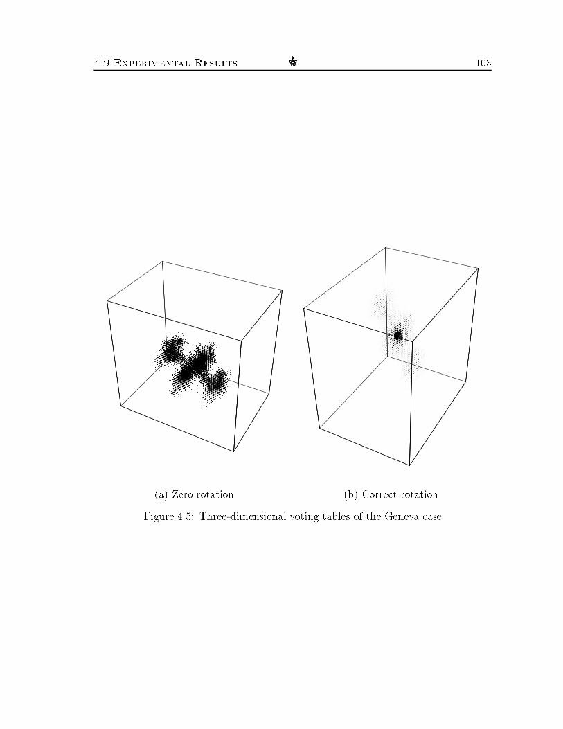
4.9 Experimental Results g 103

(a) Zero rotation (b) Correct rotationFigure 4.5: Three-dimensional voting tables of the Geneva case

104 Partial Surface and Volume Matching in Three DimensionsManhattan distance i from the point p (and considering the footprints as values ina three-dimensional domain). The motivation was to increase the sensitivity of thefootprint to the local topology around p. However, our experimentation showed amarked degradation in the performance of the algorithm. We explain this by the ob-servation that we began with discretizing the original objects into fairly large voxels,thus already distorting the object boundary by an error proportional to the voxel size.Our �rst footprint tolerated these local errors, whereas the latter footprint actuallyattempted to rely on an erroneous topology, introduced by this discretization.In the next example we looked for a partial surface match between two high-resolution depth-sensing scans of a car from two view points, obtained by a commercialdigitizer. Figures 4.6(a,b) show two `clouds' of points, which contain 119,290 and179,216 points, respectively. Because of the nature of the scanning, the two sets ofpoints describe xy-monotone surfaces (each relative to a di�erent coordinate frame).Figure 4.6(a) shows a scan of the left side of the car, as seen (in this view) frombehind the car. Figure 4.6(b) shows a scan of the front half of the car, as seen (in thisview) from the front of the car. We had no a priori data (to compare our results with)about the change of the position of the digitizer from the �rst scan to the second. Wewere informed only that the snapshots were taken when the camera was slightly tilted(i.e., took almost overhead pictures), and that the car made a \U-turn" between thetwo snapshots. Thus we expected a rotation of roughly 180 degrees about the z-axis,and small rotations about the other two axes. The amount of translation was notknown.Due to data explosion, we chose one representative point out of every 10 � 10square of points in the respective xy-grids. The representative point was simply theaverage of the coordinates of the points in the three directions. Thus, the size of thedata that we considered was only one hundredth of the original data. Figures 4.6(c,d)show the two new images from the same view points. (Each quadruple of adjacentpoints in the new grid was connected by an (almost planar) face, in order to produceshaded renderings of the surfaces.)The footprints chosen for this example aim to encode the `pyramid' of materialemanating from each vertex pi;j of the new grid of data points, and is given by thefollowing average of four spatial angles around pi;j:FP(pi;j)= 14( 6 pi�1;jpi;jpi+1;j+6 pi�1;j+1pi;jpi+1;j�1+6 pi;j+1pi;jpi;j�1+6 pi+1;j+1pi;jpi�1;j�1):This footprint distinguished well between peaks in the surface and at areas, andwas, of course, invariant under rigid motions. It turned out to be so robust, that theproximity parameter for the voting mechanism was set to only 1:0. This value wasindeed small, since the footprint was de�ned as the average of few angles speci�edin degrees. First attempts to �nd the correct rotation indicated that too many falsematches between points at nearly at regions of the surfaces contributed false votes

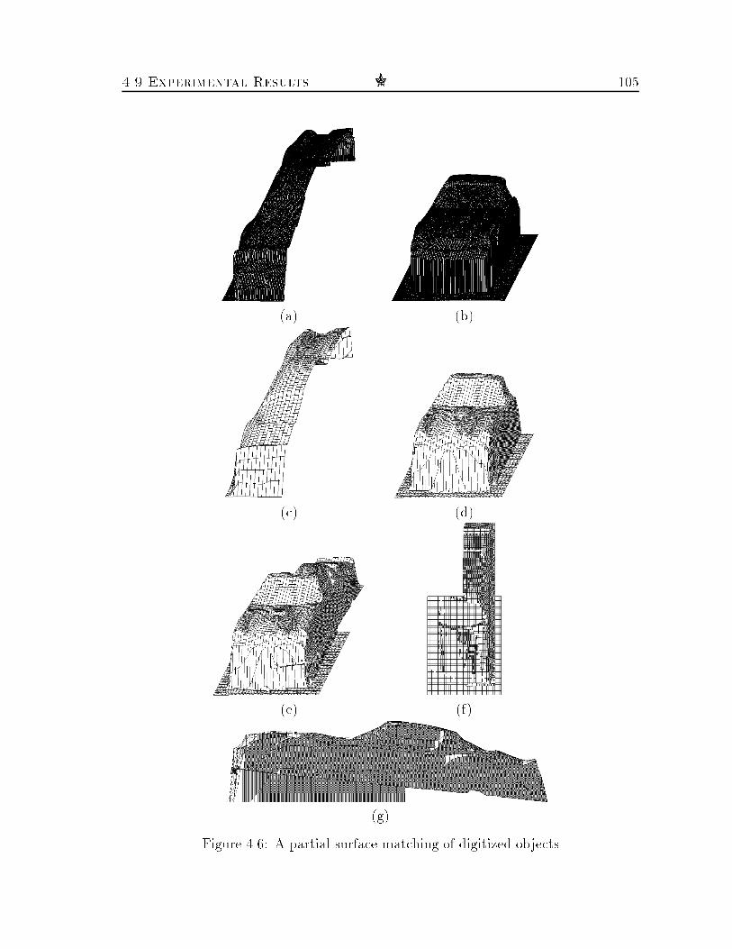
4.9 Experimental Results g 105(a) (b)(c) (d)(e) (f)(g)Figure 4.6: A partial surface matching of digitized objects

106 Partial Surface and Volume Matching in Three Dimensions

(a) Zero rotation (b) Correct rotationFigure 4.7: Three-dimensional voting tables of the Car caseto the voting tables. To �x this, we have excluded from the generic voting list all thepoints having footprints in the range 170{190 degrees. This improved the matching,and also reduced signi�cantly the running time, due to data reduction.The algorithm found the rotation (6; 4:9; 180:9) degrees, and the shift (16,41,0).Figures 4.6(e,f,g) show isometric, top, and side views, respectively, of the �rst scanimposed on the second after applying this transformation. The three �gures showthat the two surfaces match quite closely in their overlapping portions. A thirdsnapshot of the car, which partially overlapped with the second, was also matched,in a subsequent experiment, with equally good results.Figure 4.7 shows typical distributions of votes in the voting tables. Figure 4.7(a)shows the voting table that corresponds to the zero rotation, whereas Figure 4.7(b)shows the voting table that corresponds to the rotation which the algorithm found tobe correct. Again, the accumulation point that represents the correct translation iswell seen in the latter �gure. (This graphical representation is a little misleading, sinceit does not display well the density of the cluster in Figure 4.7(b). In `astrophysical'terms, the cluster is nearly a `black hole', representing about 16% of the votes.)The next several examples are from molecular biology. The �rst two of themconsist of the same input. The data describes two subunits (chains) of human de-

4.9 Experimental Results g 107oxyhemoglobin (a protein found inside red cells of the human blood), having thewell-known �-� dimer [FPSF]. This dimer is re ected by a geometric match betweenportions of the boundaries of the two subunits, with volume complementarity nearthe matched boundaries. In fact, the hemoglobin molecules contain two �-� dimerssymmetrically arranged so that each � subunit is in contact with two � subunits, oneof which is a tight contact and the other is loose [KSEF, Le]. The data was obtainedfrom the Brookhaven Protein Data Bank (Brookhaven National Laboratory, Upton,NJ), where it is denoted by 2HHB. Each molecule is given as a list of atoms andthe spatial coordinates of their centers. Figure 4.8(a) shows the two subunits (the �chain is darker), already in the docking orientation.As was mentioned in the introduction (Section 4.1), previous methods for match-ing (docking) molecules usually applied a preprocessing step, which attempts to locatethe `boundary' of the molecules, and to discard all the `inner' atoms which do notplay a role in the matching. We invoked a simple procedure which (not quite ac-curately) tried to achieve a similar e�ect. For each atom a, We checked the eightaxis-parallel octants with apex a, within L1-distance of 5 �A from a. If every oneof the eight limited octants contained at least one other atom, we considered a tobe `totally inner', and discarded it. We computed the footprint of each remaining`boundary' atom, as the `amount of material' (including inner atoms) found inside a9� 9� 9 cube centered at the atom. Speci�cally, we computed how many of the 729voxels in this cube contain the center of at least one atom. (Recall that the `volumes'of atoms connected by van der Waals bonds overlap.) Since we are interested here inmatches that have volume complementarity, we summed up the footprints of everycandidate pair of atoms, and if the result was su�ciently close to 729, then the pairof atoms was added to the generic voting list.The algorithm found the best rotation to be (�0:25; 0; 0). (We did not know inadvance that the data was given so that it already re ected the docking, namely,the correct solution that re ects the tight contact between the � and the � chainsshould have been the zero rotation and translation.) The simple technique for �ndingthe �nal translation failed, since the voting table of the correct rotation was still toosparse, and no distinguished accumulation point could be identi�ed. We feel that thishappened since we did not compute accurately enough the boundary surfaces of themolecule subunits (namely, we considered some of the `inner' atoms as being on theboundary, and erroneously discarded some of the `outer' atoms), and that the chosenfootprints were not descriptive enough. We believe, however, that the neighborhoodparameter for the voting mechanism was accurate. Given the correct rotation, weapplied a simple correlation function, similar to the function described in [KSEF] andin Section 4.7. We set cA and cB to �15 and 2, respectively. The program checked a5�A-grid of translations in the range of �30 to 30 �A in each direction, and found thecorrect translation to be (�2; 0; 1) (while the zero translation was expected).In order to verify the docking, we computed the intersection of the two molecules

108 Partial Surface and Volume Matching in Three Dimensions(a)

(b) (c)(d) (f) (h)(e) (g) (i)Figure 4.8: Full volume and partial surface matching of hemoglobin subunits

4.9 Experimental Results g 109with a series of parallel planes. Figures 4.8(b,c) show the intersections with the planeX = 14:7 (at the original world coordinates). The matching area is seen between theupper right side of (b), and the lower left side of (c). These �gures repeat the resultspresented at [KSEF].Next, we looked for a volume match between these two subunits of hemoglobin.The shapes of the two chains resembled each other, and indeed, the algorithm founda rotation and a translation, which made them almost fully overlap. Figures 4.8(d,e)show the two subunits, side by side, after applying the rotation. The two subunitsare shown in Figures 4.8(f,g) and in Figures 4.8(h,i) in the same orientation but fromdi�erent view points. These overlaps reveal structural motifs which are common tothe two chains. Indeed, the � and the � chains are very similar to each other in theirtertiary structure, which consists of similar lengths of an �-helix with bends of aboutthe same angles and directions [Le, p. 145].We applied the same procedure in order to identify a similar �-� dimer of twosubunits of horse methemoglobin (PDB code 2MHB). Here the areas of the matchingboundary portions were smaller than those in the 2HHB case. Since the initial phase(scoring a coarse grid of points in the space of rotations) gave high scores to severalrotations, we passed to the advancing phases the 5 rotations that received the highestscores. The algorithm identi�ed two signi�cant maxima of the scoring function: therotations (�1:688; 5:312; 174) and (1:875; 0; 0). The latter rotation represents thetight contact between the � and the � chains. The correlation function, in its settingfor the 2HHB case, did not score high enough the correct translation for the tightcontact. We modi�ed the cell-to-cell contribution to be 3 in case the two cells wereon the subunit boundaries, �6 in case one cell was on the boundary of one subunitand the other cell was internal to the second subunit, and �10 in case the two cellswere internal to the subunits. These values were found empirically. This versionof the correlation function found the correct translation within a very small error.Figure 4.9 shows the docking of the two methemoglobin subunits in the tight contactbetween them.We have also attempted to dock a receptor (myoglobin) with a ligand (heme).For this purpose we used myoglobin from a sperm whale (PDB code 4MBN). Fischeret al. report in [FNNW] that their docking program found 4 good solutions (outof 134) after running 2.3 minutes (CPU time) on a Silicon Graphics workstation.Our program required more time but produced very accurate results. The algorithmfound the best rotation to be (�2; 0;�2) and the corresponding translation to be(�3;�1; 4), while the expected solution was the zero transformation. Figure 4.10shows the docking of the receptor with the (darker) ligand.Finally, we applied our algorithm to the problem of registration of medical images.We compared three bit-volumes obtained by scanning a functional brain phantom withan MRI scanner. (A functional phantom is a piece of material (perspex, in our case),in which the shape of the organ is engraved. In order to simulate the scanning of the

110 Partial Surface and Volume Matching in Three Dimensions

Figure 4.9: Docking of horse methemoglobin subunits

4.9 Experimental Results g 111

Figure 4.10: Docking of a ligand (heme) into a receptor (myoglobin)

112 Partial Surface and Volume Matching in Three Dimensions(a) Original (b) Tilted by �8 degreesFigure 4.11: Surface matching of a functional brain phantomorgan in di�erent imaging modalities, such as CT, MRI, SPECT, etc., special typesof liquid (each modality with its own appropriate liquid) �ll the engraved shape ofthe organ. Every imaging modality can be tuned to be sensitive to the correspondingspecial liquid, and almost insensitive at all to the phantom itself.)In our experiment, we compared three MRI scans of the phantom. The �rst twoscans di�ered in their resolutions: the distance between consecutive slices in the �rstscan was 6 mm, whereas it was only 3 mm in the second scan. The phantom hadthe same orientation in the �rst two scans. The resolution of the third scan was ashigh as the second, but the phantom was rotated by �8 degrees around the x-axis,relative to the �rst two scans. The data obtained by the scanner were 3 bit-volumes,where the dimensions of each voxel were 0:86� 0:86 � 0:86 mm3.We faced a data-explosion problem in this experiment, too. The original bit-volumes contained 35,457, 35,898, and 36,111 points. We used only those pointswhose coordinates in the xyz-grid were integer multiples of 5. Thus, the size of thedata that we considered was reduced by a factor of roughly 125. Figures 4.11(a,b)show the �rst and the third scans of the phantom from a side view point. (The secondscan looks much the same as the �rst one.)As for the Geneva experiment, the footprints chosen for this example count the`amount of material' around each voxel. We considered only boundary voxels of the2-dimensional MRI scans (obtained by standard grey-level thresholding), and thefootprint of a voxel was set to the number of voxels belonging to the phantom within

4.9 Experimental Results g 113the 5� 5 � 5 cube centered at the given voxel. Thus, the footprint values vary from1 to 125. The proximity parameter for the voting mechanism was set to 1. Weexperimented with the three possible registrations of pairs of scans (out of the three).The algorithm found the correct rotation and translation in all the three experimentswith practically no error at all. The results are detailed in Table 4.1.Table 4.1 summarizes the performance of our implementation on all the examplesdescribed above, except for the molecule docking. The latter experiments are summa-rized in Table 4.2. In all the docking experiments we sought a surface matching, thefootprint was the same as for the volume matching of the molecules (see Table 4.1),and the correct rotation and translation were the identity. All the time measurementsin Tables 4.1 and 4.2 were taken on an SGI Indigo workstation. Our experimentalresults show that the time needed for a scoring operation primarily depended onthe number of voting pairs and on the average density of the voting tables, whichdepends more on the particular matching instance and less on the speci�c rotation.This was re ected well in the molecule docking experiments, in which a scoring op-eration usually required more time than in the other experiments, due to the largersparseness of the voting tables in this case. The total running time for a speci�cinstance depended roughly linearly on the number of scoring operations, since thedi�erence (in running time) between di�erent scoring operations for the same datawas not signi�cant. Typically, the third phase of the algorithm required signi�cantlymore time than the second phase (except for the Geneva case). In practice, however,the third phase could be omitted, because the results of the second phase were ac-curate enough and the improvement of the third phase was relatively small. Each ofour experiments took a few minutes to run. However, we can trade time for accuracy,by reducing the proximity parameter (thereby reducing the number of voting pairs),by reducing the resolution of the xyz-grid (thereby making the voting tables denser),and/or by reducing the resolution of the search in 3-dimensional space of rotations(thereby reducing the number of scoring operations).We have also implemented the statistical method described in Section 4.8 andapplied it to the matching of the snapshots of the car mentioned earlier in this sec-tion. The principal components analysis revealed the characteristic values 170.54,24.53, and 8.40, with the corresponding characteristic vectors (0:012; 0:999;�0:045),(0:994;�0:008; 0:105), and (�0:105; 0:046; 0:993), respectively. The third character-istic vector was thus in the direction of the axis of rotation `. We then projected thetwo data sets on a plane orthogonal to `, and computed the relative rotation betweenthe projected sets according to the method described in Section 4.8.3 (the resultingangle was 179.0125). Putting everything together, we got that the rotational com-ponent of the correct transformation was R = 0B@ �0:978 �0:024 �0:2070:010 �0:997 0:071�0:208 0:067 0:976 1CA. (Allthe computations were performed in a much higher precision than the one shown

114 Partial Surface and Volume Matching in Three DimensionsMatching Prox. VotingCase Type jAj jBj Footprint Param. PairsGeneva Volume 553 552 # of voxels in a 5-box 1 16,721Car Surface 1,1851 1,7281 Spatial angles 1.0 13,609Molecules Volume 1,1122 1,1662 # of occupied �A3-cells 4 6,242(2HHB) in a 9 � 9� 9 boxPhantom Surface 277 272 # of occupied 1 4,236Surface 277 295 cells in a 1 4,432Surface 272 295 5� 5� 5 box 1 4,476Correct CorrectCase Rotation TranslationGeneva (15:7; 115:2; 200:1) (3; 11; 20)Car Unknown UnknownMolecules (2HHB) Unknown UnknownPhantom (1 & 2) (0:0; 0:0; 0:0) (0; 0; 0)Phantom (1 & 3) (�8:0; 0:0; 0:0) ~(0; 0; 0)Phantom (2 & 3) (�8:0; 0:0; 0:0) ~(0; 0; 0)Computed Rotation ComputedCase Phase II Phase III TranslationGeneva (16:0; 116:0; 200:0) (16:0; 115:625; 200:875) (3; 11; 20)Car3 (6:0; 4:0; 182:0) (6:000; 4:875; 180:875) (16; 41; 0)Molecules (2HHB) (0:0; 180:0; 180:0) (�0:125; 181:0; 181:375) (1;�2; 2)Phantom (1 & 2)4 (0:0; 0:0; 0:0) (0:0; 0:0; 0:0) (0; 0; 0)Phantom (1 & 3)4 (�8:0; 0:0; 0:0) (�8:25;�0:25; 0:0) (0;�1; 2)Phantom (2 & 3)4 (�8:0; 0:0; 0:0) (�8:00; 1:5; 1:0) (0;�1; 2)# of Scoring Operations Time (Sec.)Case I II III Total I II III Total Per S.O.Geneva 108 288 270 666 57 146 137 340 0.51Car 108 108 162 378 56 53 79 188 0.50Mol. (2HHB) 108 72 288 468 87 58 233 378 0.81Pha. (1 & 2) 108 36 54 198 61 20 27 108 0.55Pha. (1 & 3) 108 72 126 306 60 36 73 169 0.55Pha. (2 & 3) 108 72 108 288 56 41 64 161 0.551433 and 605, respectively, after omitting ` at' points.2473 and 480, respectively, after eliminating `inner' points.3In this experiment dmin was set to 0.25.4In these experiments dmax was set to 8.0.Table 4.1: Performance of the matching algorithm

4.9 Experimental Results g 115Prox. VotingCase jAj jBj Param. Pairs2HHB 1,1121 1,1661 30 5602MHB 1,1132 1,1782 30 3574MBN 443 1,3393 30 823# of Initial Computed Rotations ComputedCase Starting Points Phase II Phase III Translations2HHB 1 (0:0; 0:0; 0:0) (�0:25; 0:0; 0:0) (-2,0,1)42MHB 5 (2:0; 0:0; 2:0) (1:875; 0:0; 0:0) (1; 0;�1)44MBN 2 (�2:0; 0:0;�2:0) (�1:688; 0:562;�1:75) (�3;�1; 4)# of Scoring Operations Time (Sec.)Case I II III Total I II III Total Per S.O.2HHB 108 54 126 288 80 40 94 214 0.742MHB 108 162 450 720 73 112 310 495 0.684MBN 108 162 324 594 88 134 273 495 0.831473 and 480, respectively, after eliminating `inner' points.2479 and 498, respectively, after eliminating `inner' points.335 and 553, respectively, after eliminating `inner' points.4Translation computed by the correlation technique; its timing is not included here.Table 4.2: Performance of the matching algorithm on molecule docking

116 Partial Surface and Volume Matching in Three Dimensionshere.) This compares to the rotation matrix 0B@ �0:996 0:006 �0:086�0:015 �0:995 0:103�0:085 0:104 0:991 1CA that wegot with the regular method. We did not need to further advance from this rotationto better rotations. The running time on an SGI Indigo workstation was the follow-ing: the principal components analysis required 2 seconds, projecting the data ontoa 2-dimensional problem was negligible, solving the 2-dimensional problem required16 additional seconds, and obtaining the �nal rotational component of the solutionwas again negligible. Thus, in total, the statistical approach required 18 seconds inthis case, compared with 188 seconds for the regular method. We did not achieveadequate results in any other of our experiments with the statistical method.4.10 ConclusionWe have proposed in this chapter an algorithm for solving the practical problem ofpartial surface or volume matching between two objects in 3-space. This problem is abasic and important problem in pattern recognition and computer vision, with manyindustrial, biological, and medical applications.We have treated separately the rotation and the translation components of therelative rigid motion between the two objects. We developed a two-step technique(voting followed by scoring the vote) for measuring the goodness of a given rotation,then used this technique as a subroutine called by an iterative process that advancestowards the best rotation. Finally, we computed the best translation between theobjects, corresponding to the best rotation. We used footprints which counted the`amount of material' for volumematching, and surface-curvature footprints for surfacematching.As demonstrated, our technique found accurately the matchings between severalpairs of objects, taken from several totally di�erent domains. A manual inspec-tion of the resulting voting tables shows that they are fairly noisy. The typical tablelooks like a cloud of randomly and sparsely (though not necessarily uniformly) spreadpoints, containing a small slightly dense region where the good votes are clustered.It is rather miraculous that our technique did manage to score such tables properly.One of the open problems that we pose for future research is to develop alternativetheoretically-sound and practically-e�cient methods for identifying such clusters ofdata in otherwise randomly spread data. As already remarked, the statistical litera-ture that we are aware of does not seem to provide such a technique.There are several research directions that we plan to pursue and to explore further.We plan to continue the experimentation with our algorithm, to test its performancelimits and see if there are data instances on which the algorithm needs further �ne-tuning to perform well. We plan to experiment with more pairs of protein molecules

4.10 Conclusion g 117and with other types of data.We also plan to explore several enhancements and improvements of the algorithm.These include the design of better footprints (especially in the molecular biologydomain), experimentation with other scoring functions, further study of the statisticalapproach, design of better searching mechanisms, etc.We plan to improve the implementation of the voting parameters in the moleculedocking problem. Speci�cally, we plan to improve the determination of the atoms onthe boundaries of the molecules, and to try to compute better footprints for them.Moreover, we plan to enhance the footprints, so that they re ect not only the geome-tries of the molecules, but also chemical properties of the atoms, such as their bases,electrical potentials, possible connections, etc., which also play a signi�cant role inthe chemical reaction between molecules. Assuming that all this can be achievedsuccessfully, a longer-range project is to apply our algorithm en masse to existingdata banks of proteins and other macromolecules, as a tool for automatic drug designand for general study of the geometric structure of proteins.

Chapter 5Concluding Remarks and FuturePlansIn this research we have presented several applications of the geometric hashingtechnique. We have shown its applicability to problems involving partial match-ing of curves, surfaces, or volumes in two and three dimensions. We concentrated onthree practical problems, which arise in several rather di�erent domains. While the�rst problem from the CAD world (gap �lling) has attracted only little attention inthe past, the two other problems, namely solid reconstruction from polygonal slices(mostly out of medical data) and surface or volume matching in three dimensions,have a long history of previous work in pattern recognition, industrial applications,medical imaging, and molecular biology. We consider our results to be new and im-proved approaches for all these problems. Comparing our experimentations with theearlier works in the published literature, our solutions appear to be more general,more robust, and often faster than previous techniques.The geometric hashing technique has been proven to be very robust in practice.While it is only a heuristic, whose implementation should be tuned separately fordi�erent applications or even for di�erent classes of instances of the same application,our experimentation shows that this tuning is very easy in most cases, and that awide range of tuning parameters produce very good results.We plan to continue the experimentation with the reconstruction software, to testits performance limits and see if there are data instances on which the algorithmmight not perform well, thus requiring further calibrations and enhancements. Forthis purpose, we have initiated a database, which contains a large collection of polygo-nal slice data, including many human organs, topographic maps, and sliced industrialmodels. This database was created in cooperation with B. Wolfers from Freie Univer-sit�at Berlin. We plan to create a testbed for comparing competitive reconstructionalgorithms. We also plan to bring the reconstruction software to a (nearly) industrial119

120 Concluding Remarks and Future Planslevel, including a graphic interface, programmable user-de�ned defaults, a variety ofinput and output �le formats, etc. Our hope is to get our software to be used inactual commercial systems.Other future plans are to further extend our work on the surface matching problemand on its applications in identifying geometric �ts between the boundaries of pairs ofmacromolecules (mainly for the molecule docking problem). Important applicationsof this research are the recognition and binding of receptors and ligands in proteins,and synthetic drug design. Speci�cally, we will attempt to enhance the computationof the molecule boundaries, to choose more `descriptive' footprints (for reducing theamount of noise in the voting process and for improving the recognition accuracy),to improve the scoring function, and to make it more concrete, so as to point at thematching portions of the surfaces. The end-product will be a software package at anindustrial, or near-industrial, level, plus extensive experimentation with this software.Again, we hope to get this software to be used in real commercial applications.

Bibliography[An] T.W. Anderson, An Introduction to Multivariate Statistical Analysis, John Wiley &Sons, Inc., 1958.[ABKC] N.M. Alpert, J.F. Bradshaw, D. Kennedy, and J.A. Correia, The principal axestransformation|A method for image registration, J. of Nuclear Medicine, 31 (1990),1717{1722.[AHB] K.S. Arun, T.S. Huang, and S.D. Blostein, Least square �tting of two 3-D pointsets, IEEE Trans. on Pattern Analysis and Machine Intelligence, 9 (1987), 698{700.[AM1] R.A. Abagyan and N.V. Maiorov, A simple qualitative representation of polypeptidechain folds: Comparison of protein tertiary structures, J. of Biomolecular Structure andDynamics, 5 (1988), 1267{1279.[AM2] T. Abel and T. Maniatis, Gene regulation: Action of leucine zippers, Nature, 341(1989), 24{25.[Ba] D.H. Ballard, Generalizing the Hough transform to detect arbitrary shapes, PatternRecognition, 13 (1981), 111-122.[Be1] P.J. Besl, Geometric modeling and computer vision, Proc. IEEE, 76 (1988), 936{958.[Be2] P.J. Besl, The free-form surface matching problem, in: Machine Vision for Three-Dimensional Scenes (H. Freeman, ed.), New York: Academic, 1990.[Bo1] J.D. Boissonnat, Shape reconstruction from planar cross sections, Computer Vision,Graphics and Image Processing, 44 (1988), 1{29.[Bo2] F.L. Bookstein, From medical images to the biometrics of form, in: Information Pro-cessing in Medical Imaging (S.L. Bacharach, ed.), Martinus Nijho� Publishers, Dor-drecht, the Netherlands, 1986, 1{18.[Bo3] F.L. Bookstein, Thin-plate splines and the atlas problem for biomedical images, in:Information Processing in Medical Imaging (A.C.F. Colchester and D.J. Hawkes, eds.),Springer-Verlag, Berlin, 1991, 326{342.[Bo4] G. Borgefors, An improved version of the chamfer matching algorithm, Proc. 7th Int.Conf. on Pattern Recognition, 1984, 1175{1177.[Bo5] G. Borgefors, Hierarchical chamfer matching: A parametric edge matching algorithm,IEEE Trans. on Pattern Analysis and Machine Intelligence, 10 (1988), 849{865.121

122 g BIBLIOGRAPHY[Br1] P. Brou, Using the Gaussian image to �nd the orientation of an object, Int. J. ofRobotics Research, 3 (1983), 89{125.[Br2] L.G. Brown, A survey of image registration techniques, ACM Computing Surveys, 24(1992), 325{376.[BA] B.A. Boyter and J.K. Aggarwal, Recognition with range and intensity data, Proc.Workshop on Computer Vision: Representation and Control, IEEE, Annapolis, MD,1984, 112{117.[BC] R.C. Bolles and R.A. Cain, Recognizing and locating partially visible objects: Thelocal-feature-focus method, Int. J. of Robotics Research, 1 (1982), 57{82.[BG] J.D. Boissonnat and B. Geiger, Three dimensional reconstruction of complex shapesbased on the Delaunay triangulation, Technical Report 1697, INRIA, Sophia Antipolis,France, 1992.[BH] R.C. Bolles and P. Horaud, 3DPO: Three-dimensional part orientation system, Int.J. of Robotics Research, 5 (1986), 3{26.[BJ1] P.J. Besl and R.C. Jain, Three-dimensional object recognition, ACM ComputingSurveys, 17 (1985), 75{154.[BJ2] F.P. Beer and E.R. Johnston, Jr., Vector Mechanics for Engineers: Dynamics,McGraw-Hill, 1986.[BK] R. Bajcsy and S. Kova�ci�c, Multiresolution elastic matching, Computer Vision,Graphics, and Image Processing, 46 (1989), 1{21.[BM] P.J. Besl and N.D. McKay, A method for registration of 3-D shapes, IEEE Trans.on Pattern Analysis and Machine Intelligence, 14 (1992), 239{256.[BPCC] S. Batnitzky, H.I. Price, P.N. Cook, L.T. Cook, and S.J. Dwyer III, Three-dimensional computer reconstruction from surface contours for head CT examinations,J. of Computer Assisted Tomography, 5 (1981), 60{67.[BS1] G. Barequet and M. Sharir, Filling gaps in the boundary of a polyhedron,Computer-Aided Geometric Design, to appear.[BS2] G. Barequet and M. Sharir, Piecewise-linear interpolation between polygonal slices,Proc. 10th ACM Symp. on Computational Geometry, 1994, 93{102; also to appear inComputer Vision, Graphics, and Image Processing: Image Understanding.[BS3] G. Barequet and M. Sharir, Partial surface and volume matching in three dimen-sions, Proc. 12th IAPR and IEEE Int. Conf. on Pattern Recognition, 1994, to appear.[BTBW] H.G. Barrow, J.M. Tenenbaum, R.C. Bolles, and H.C. Wolf, Parametric cor-respondence and chamfer matching: Two new techniques for image matching, Proc. 5thInt. Joint Conf. on Arti�cial Intelligence, 1977, 659{663.[BW] J.H. B�hn and M.J. Wozny, Automatic CAD-model repair: Shell-closure, Proc.Symp. on Solid Freeform Fabrication, Dept. of Mech. Eng., Univ. of Texas at Austin,1992, 86{94.

BIBLIOGRAPHY g 123[BY] A. Blake and A. Yuille, Active Vision, MIT Press, Cambridge, MA, 1993.[Ch] B. Chazelle, A functional approach to data structures and its use in multidimensionalsearching, SIAM J. of Computing, 17 (1988), 427{462.[Co1] M.L. Connolly, Analytical molecular surface calculation, J. of Applied Crystallogra-phy, 16 (1983), 548{558.[Co2] M.L. Connolly, Solvent-accessible surfaces of proteins and nucleic acids, Science, 221(1983), 709{713.[Co3] M.L. Connolly, Shape complementarity at the hemoglobin �1-�1 subunit interface,Biopolymers, 25 (1986), 1229{1247.[CCLB] L.T. Cook, P.N. Cook, K.R. Lee, S. Batnitzky, B.Y.S. Wong, S.L. Fritz, J.Ophir, S.J. Dwyer III, L.R. Bigongiari, and A.W. Tempelton, An algorithmfor volume estimation based on polyhedral approximation, IEEE Trans. on BiomedicalEngineering, 27 (1980), 493{500.[CCMM] E. de Castro, G. Cristini, A. Martelli, C. Morandi, and M. Vascotto, Com-pensation of random eye motion in television ophthalmoscopy: Preliminary results, IEEETrans. on Medical Imaging, 6 (1987), 74{81.[CD] R.T. Chin and C.R. Dyer, Model-based recognition in robot vision, ACM Computingsurveys, 18 (1986), 67{108.[CLLC] H.E. Cline, W.E. Lorensen, S. Ludke, C.R. Crawford, and B.C. Teeter, Twoalgorithms for the three-dimensional reconstruction of tomograms, Medical Physics, 15(1988), 320{327.[CPCC] C.T. Chen, C.A. Pelizzari, G.T.Y. Chen, M.D. Cooper, and D.N. Levin, Imageanalysis of PET data with the aid of CT and MR images, in: Information Processing inMedical Imaging (C.N. de Graaf and M.A. Viergever, eds.), Plenum Press, New York,1988, 601{611.[CPDE] D.L. Collins, T.M. Peters, W. Dai, and A.C. Evans, Model based segmentationof individual brain structures fromMRI data, in: Proc. SPIE Visualization in BiomedicalComputing (R.A. Robb, ed.), 1808, SPIE Press, Bellingham, WA, 1992, 10{23.[CPE] D.L. Collins, T.M. Peters, and A.C. Evans, Multiresolution image registrationand brain structure segmentation, Proc. 14th Ann. IEEE Int. Conf. on Engineering inMedicine and Biology, IEEE Computer Soc. Press, Los Alamitos, CA, 1992.[CS] H.N. Christiansen and T.W. Sederberg, Conversion of complex contour line de�-nitions into polygonal element mosaics, Computer Graphics, 13 (1978), 187{192.[DM] A. Dolenc and I. M�akel�a, Optimized triangulation of parametric surfaces, in:Computer-Aided Surface Geometry and Design (Mathematics of Surfaces IV) (A.Bowyer, ed.), 48, Clarendon Press (Oxford), 1994, 169{183.[EMCP] A.C. Evans, S. Marrett, L. Collins, and T.M. Peters, Anatomical-functionalcorrelative analysis of the human brain using three dimensional imaging systems, in:Proc. SPIE Medical Imaging III: Image Processing (R.H. Schneider, S.J. Dwyer III, andJ.R. Gilbert, eds.), 1092, SPIE Press, Bellingham, WA, 1989, 264{274.

124 g BIBLIOGRAPHY[EMPV] P.A. van der Elsen, J.B.A. Maintz, E.J.D. Pol, and M.A. Viergever, Imagefusion using geometrical features, in: Proc. SPIE Visualization in Biomedical Computing(R.A. Robb, ed.), 1808, SPIE Press, Bellingham, WA, 1992, 172{186.[EMV] P.A. van der Elsen, J.B.A. Maintz, and M.A. Viergever, Geometry drivenmultimodality image matching, Brain Topography, 5 (1992), 153{158.[EPO] A.B. Ekoule, F.C. Peyrin, and C.L. Odet, A triangulation algorithm from arbi-trary shaped multiple planar contours, ACM Trans. on Graphics, 10 (1991), 182{199.[EPV] P.A. van der Elsen, E.J.D. Pol, and M.A. Viergever, Medical image matching|A review with classi�cation, IEEE Engineering in Medicine and Biology, 12 (1993),26{39.[Fa] O.D. Faugeras, New steps toward a exible 3-D vision system for robotics, Proc. IEEE7th Int. Conf. on Pattern Recognition, 1984, 796{805.[Fi1] R.B. Fisher, Using surfaces and object models to recognize partially obscured objects,Proc. 8th Int. Joint Conf. on Arti�cial Intelligence, 1983, 989{965.[Fi2] D. Fischer, Structural Matching Algorithms in Molecular Biology, Ph.D. Thesis, Dept.of Computer Science, Tel Aviv Univ., Israel, 1993.[FBNW] D. Fischer, O. Bachar, R. Nussinov, and H.J. Wolfson, An e�cient computervision based technique for detection of three dimensional structural motifs in proteins,J. of Biomolecular Structure and Dynamics, 9 (1992), 769{789.[FD] J.D. Foley and A. van Dam, Fundamentals of Interactive Computer Graphics, Addi-son Wesley, Reading, MA, 1984.[FH] O.D. Faugeras and M. Hebert, A 3-D recognition and positioning algorithm usinggeometrical matching between primitive surfaces, Proc. 7th Int. Joint Conf. on Arti�cialIntelligence, 1983, 996{1002.[FHKL] T.J. Fang, Z.H. Huang, L.N. Kanal, B. Lambird, D. Lavine, G. Stockman, andF.L. Xiong, Three-dimensional object recognition using a transformation clusteringtechnique, Proc. 6th IAPR and IEEE Int. Conf. on Pattern Recognition, 1982, 678{681.[FKU] H. Fuchs, Z.M. Kedem, and S.P. Uselton, Optimal surface reconstruction fromplanar contours, Comm. of the ACM, 20 (1977), 693{702.[FNNW] D. Fischer, R. Norel, R. Nussinov, and H.J. Wolfson, 3-D docking of proteinmolecules, Proc. 4th Symp. on Combinatorial Pattern Matching, Lecture Notes in Com-puter Science, 684, Springer Verlag, Berlin, 1993, 20{34.[FNW] D. Fischer, R. Nussinov, and H.J. Wolfson, 3-d substructure matching in pro-tein molecules, Proc. 3rd Symp. on Combinatorial Pattern Matching, Lecture Notes inComputer Science, 644, Springer Verlag, Berlin, 1992, 136{150.[FPSF] G. Fermi, M.F. Perutz, B. Shaanan, and R. Fourme, The crystal structure ofhuman deoxyhemoglobin at 1.74�A resolution, J. of Molecular Biology, 175 (1984), 159{174.

BIBLIOGRAPHY g 125[Ge] B. Geiger, Construction et Utilisation des Mod�eles d'Organes en vue de l'Assistance auDiagnostic et aux Interventions Chirurgicals, Ph.D. Thesis, L'Ecole des Mines de Paris,1993.[Go] H. Goldstein, Classical Mechanics, Addison-Wesley, Reading, MA, 1980.[GD] S. Ganapathy and T.G. Dennehy, A new general triangulation method for planarcontours, ACM Trans. on Computer Graphics, 16 (1982), 69{75.[GF] B.A. Galler and M.J. Fischer, An improved equivalence algorithm, Comm. of theACM, 7 (1964), 301{303.[GFC] A. Gamboa-Aldeco, L.L. Fellingham, and G.T.Y. Chen, Correlation of 3D sur-faces from multiple modalities in medical imaging, in: Proc. SPIE Medicine XIV/PACSIV (R.H. Schneider and S.J. Dwyer III, eds.), 626, SPIE Press, Bellingham, WA, 1986,467{473.[GGC] G. Garibotto, C. Giorgi, and U. Cerchiari, 3-D image processing in functionalstereotactic neurosurgery, in: Proc. SPIE Applications of Digital Image Processing, 397,SPIE Press, Bellingham, WA, 1983, 280{287.[GJ] M.R. Garey and D.S. Johnson, Computers and Intractability, A Guide to the Theoryof NP-Completeness, Freeman and Co., San Francisco, 1979.[GL] G.H. Golub and C.F. van Loan, Matrix Computations, Johns Hopkins Univ. Press,Baltimore, MD, 1983.[GOS] C. Gitlin, J. O'Rourke, and V. Subramanian, On reconstructing polyhedrafrom parallel slices, Technical Report 025, Dept. of Computer Science, Smith College,Northampton, MA, 1993.[GS] L. Guibas and J. Stolfi, Primitives for the manipulation of general subdivisions andthe computation of Voronoi diagrams, ACM Trans. on Graphics, 4 (1985), 74{123.[Ho1] K. Ho-Le, Finite element mesh generation methods: A review and classi�cation,Computer-Aided Design, 20 (1988), 27{38.[Ho2] B.K.P. Horn, Extended Gaussian images, Proc. IEEE, 72 (1984), 1656{1678.[Ho3] B.K.P. Horn, Closed-form solution of absolute orientation using unit quaternions, J.of Opt. Soc. Amer., 4 (1987), 629{642.[HBGJ] D.R. Haynor, A.W. Borning, B.A. Griffin, J.P. Jacky, I.J. Kalet, and W.P.Shuman, Radiotherapy planning: Direct tumor location on simulation and port �lmsusing CT, Radiology, 158 (1986), 537{540.[HH] B.K.P. Horn and J.G. Harris, Rigid body motion from range image sequences,Computer Vision, Graphics, and Image Processing, 1989.[HHCG] D.L.G. Hill, D.J. Hawkes, J.E. Crossman, M.J. Gleeson, T.C.S. Cox,E.C.M.L. Bracey, A.J. Strong, and P. Graves, Registration of MR and CT im-ages for skull base surgery using point-like anatomical features, British J. of Radiology,64 (1991), 1030{1035.

126 g BIBLIOGRAPHY[HHH] D.L.G. Hill, D.J. Hawkes, and C.R. Hardingham, The use of anatomical knowl-edge to register 3D blood vessel data derived from DSA with MR images, in: Proc. SPIEImage Processing, 1445, SPIE Press, Bellingham, WA, 1991, 348{357.[HHLR] D.J. Hawkes, D.L.G. Hill, E.D. Lehmann, G.P. Robinson, M.N. Maisay, andA.C.F. Colchester, Preliminary work on the interpretation of SPECT images withthe aid of registered MR images and an MR derived 3D neuro-anatomical atlas, in: 3DImaging in Medicine (K.H. H�ohne, H. Fuchs, and S.M. Pizer, eds.), Springer-Verlag,Berlin, 1990, 241{251.[HKR] D.P. Huttenlocher, G.A. Klanderman, and W.J. Rucklidge, Comparing im-ages using the Hausdor� distance, Technical Report CUCS-TR-91-1211, Dept. of Com-puter Science, Cornell Univ., Ithaca, NY, 1991; also to appear in IEEE Trans. on PatternAnalysis and Machine Intelligence.[HNR] D.P. Huttenlocher, J.J. Noh, and W.J. Rucklidge, Tracking non-rigid objectsin complex scenes, Proc. IEEE Int. Conf. on Computer Vision, 1993.[HO] D. Halperin and M. Overmars, Spheres, molecules, and hidden surface removal,Proc. 10th ACM Symp. on Computational Geometry, 1994, 113-122.[HU1] D.P. Huttenlocher and S. Ullman, Object recognition using alignment,Proc. IEEEConf. on Computer Vision, 1987, 102-111.[HU2] D.P. Huttenlocher and S. Ullman, Recognizing solid objects by alignment withan image, Int. J. of Computer Vision, 5 (1990), 195{212.[HW] J. Hong and H.J. Wolfson, An improved model-based matching method using foot-prints, Proc. 9th Int. Conf. on Pattern Recognition, 1988, 72{78.[JHR] H. Jiang, K. Holton, and R. Robb, Image registration of multimodality 3-D medicalimages by chamfer matching, in: Proc. SPIE Biomedical Image Processing and Three-Dimensional Microscopy, 1660, SPIE Press, Bellingham, WA, 1992, 356{366.[JK] F. Jiang and S.H. Kim, Soft docking: Matching of molecular surface cubes, J. ofMolecular Biology, 219 (1991), 79{102.[JMHB] L. Junck, J.G. Moen, G.D. Hutchins, M.B. Brown, and D.E. Kuhl, Correlationmethods for the centering, rotation, and alignment of functional brain images, J. ofNuclear Medicine, 31 (1990), 1220{1226.[JRH] H. Jiang, R.A. Robb, and K.S. Holton, A new approach to 3-D registration ofmultimodality medical images by surface matching, in: Proc. SPIE Visualization inBiomedical Computing (R.A. Robb, ed.), 1808, SPIE Press, Bellingham, WA, 1992,196{213.[Ka] R.M. Karp, Reducibility among combinatorial problems, in: Complexity of ComputerComputations (R.E. Miller and J.W. Thatcher, eds.), Plenum Press, New York, 1972,85{103.[Ke] E. Keppel, Approximating complex surfaces by triangulation of contour lines, IBM J.of Research and Development, 19 (1975), 2{11.

BIBLIOGRAPHY g 127[Kl] G.T. Klincsek, Minimal triangulations of polygonal domains,Annals of Discrete Math-ematics, 9 (1980), 121{123.[KBOL] I.D. Kuntz, J.M. Blaney, S.J. Oatley, R. Langridge, and T.E. Ferrin, Ageometric approach to macromolecule-ligand interactions, J. of Molecular Biology, 161(1982) 269{288.[KCF] F.S. Kuhl, G.M. Crippen, and D.K. Friesen, A combinatorial algorithm for calcu-lating ligand binding, Computational Chemistry, 5 (1984), 24{34.[KD] N. Kehtarnavaz and R.J.P. de Figueiredo, A framework for surface reconstructionfrom 3D contours, Computer Vision, Graphics and Image Processing, 42 (1988), 32{47.[KDVE] P.A. Kenny, D.J. Dowsett, D. Vernon, J.T. Ennis, A technique for digital imageregistration used prior to subtraction of lung images in nuclear medicine, Physical MedicalBiology, 35 (1990), 679{685.[KGCR] S. Kova�ci�c, J.C. Gee, W.S.L. Ching, M. Reivich, and R. Bajcsy, Three-dimensional registration of PET and CT images, Proc. 11th Ann. IEEE Int. Conf. onEngineering in Medicine and Biology, IEEE Computer Soc. Press, Los Alamitos, CA,1989, 548{549.[KGV] S. Kirkpatrick, C.D. Gelatt, Jr., and M.P. Vecchi, Optimization by simulatedannealing, Science, 220 (1983), 671{680.[KHW] E. Kishon, T. Hastie, and H. Wolfson, 3-D curve matching using splines, J. ofRobotic systems, 8 (1991), 723{743.[KJR] B. Kamgar-Parsi, J.L. Jones, and A. Rosenfeld, Registration of multiple overlap-ping range images: Scenes without distinctive features, Proc. IEEE Conf. on ComputerVision and Pattern Recognition, 1989.[KSD] N. Kehtarnavaz, L.R. Simar, and R.J.P. de Figueiredo, A syntactic/semantictechnique for surface reconstruction from cross-sectional contours, Computer Vision,Graphics and Image Processing, 42 (1988), 399{409.[KSEF] E. Katchalski-Katzir, I. Shariv, M. Eisenstein, A.A. Friesem, C. Aflalo, andI.A. Vakser, Molecular surface recognition: Determination of geometric �t betweenproteins and their ligands by correlation techniques, Proc. National Academy of Sciencesof the USA (Biophysics), 89 (1992), 2195{2199.[KSSS] A. Kalvin, E. Schonberg, J.T. Schwartz, and M. Sharir, Two-dimensional,model-based, boundary matching using footprints, Int. J. of Robotics Research, 5 (1986),38{55.[Le] A.L. Lehninger, Biochemistry, Worth Publishers, Inc., New York, 1978.[LC] W.E. Lorensen and H.E. Cline, Marching cubes: A high resolution 3D surfaceconstruction algorithm, Computer Graphics, 21 (1987), 163{169.[LHD] S. Linnainmaa, D. Harwood, and L.S. Davis, Pose determination of a three-dimensional object using triangle pairs, IEEE Trans. on Pattern Analysis and MachineIntelligence, 10 (1988), 634{647.

128 g BIBLIOGRAPHY[LSW1] Y. Lamdan, J.T. Schwartz, and H.J. Wolfson, On recognition of 3-d objects from2-d images, Proc. IEEE Int. Conf. on Robotics and Automation, 1988, 1407{1413.[LSW2] Y. Lamdan, J.T. Schwartz, and H.J. Wolfson, A�ne invariantmodel-based objectrecognition, IEEE Trans. on Robotics and Automation, 6 (1990), 578{589.[LW1] Y. Lamdan and H.J. Wolfson, Geometric hashing: A general and e�cient model-based recognition scheme, Proc. IEEE Int. Conf. on Computer Vision, 1988, 238{249.[LW2] Y. Lamdan and H.J. Wolfson, On the error analysis of geometric hashing, Proc.IEEE Conf. on Computer Vision and Pattern Recognition, 1991, 22{27.[Me1] N. Megiddo, Applying parallel computation algorithms in the design of serial algo-rithms, J. of the ACM, 30 (1983), 852{865.[Me2] K. Mehlhorn, Data Structures and Algorithms 3: Multi-Dimensional Searching andComputational Geometry (W. Brauer, G. Rozenberg, and A. Salomaa, eds.), Springer-Verlag, Berlin, 1984.[Mo] M. Moshfeghi, Elastic matching of multimodality medical images, CVGIP: GraphicalModels and Image Processing, 53 (1991), 271{282.[MARW] E.M. Mitchel, P.J. Artymiuk, D.W. Rice, and P. Willet, Use of techniquesderived from graph theory to compare secondary structure motifs in proteins, J. ofMolecular Biology, 212 (1989), 151{166.[MD] I. M�akel�a and A. Dolenc, Some e�cient procedures for correcting triangulated mod-els, Proc. Symp. on Solid Freeform Fabrication, Dept. of Mech. Eng., Univ. of Texas atAustin, 1993, 126{134.[MFP] V.R. Mandava, J.M. Fitzpatrick, and D.R. Pickens III, Adaptive search spacescaling in digital image registration, IEEE Trans. on Medical Imaging, 8 (1989), 251{262.[MK] H. M�uller and A. Klingert, Surface interpolation from cross sections, in: Focus onScienti�c Visualization (H. Hagen, H. M�uller, and G.M. Nielson, eds.), Springer Verlag,Berlin, 1993, 139{189.[MSS] D. Meyers, S. Skinner, and K. Sloan, Surfaces from contours: The correspondenceand branching problems, Proc. Graphics Interface '91, 1991, 246{254.[NIST] National Institute of Standards and Technology (NIST), The Initial GraphicsExchange Speci�cation (IGES), Version 5.1, MD, 1991.[NW] R. Nussinov and H.J. Wolfson, E�cient detection of three-dimensional struc-tural motifs in biological macromolecules by computer vision techniques, Proc. NationalAcademy of Sciences of the USA (Biophysics), 88 (1991), 10495{10499.[Po1] M. Potmesil, Generation of 3D surface descriptions from images of pattern-illuminatedobjects, Proc. IEEE Conf. on Pattern Recognition and Image Processing, 1979, 553{559.[Po2] M. Potmesil, Generating models of solid objects by matching 3D surface segments,Proc. 8th Int. Joint Conf. on Arti�cial Intelligence, 1983, 1089{1093.[Pr] W.K. Pratt, Digital Image Processing, Wiley, NY, 1978.

BIBLIOGRAPHY g 129[PCSW] C.A. Pelizzari, G.T.Y. Chen, D.R. Spelbring, R.R. Weichselbaum, and C.T.Chen, Accurate three-dimensional registration of CT, PET, and/or MR images of thebrain, J. of Computer Assisted Tomography, 13 (1989), 20{26.[Ri] F.M. Richards, Areas, volumes, packing and protein structure, Ann. Rev. Biophysicsand Bioengineering, 6 (1977), 151{176.[RK] F.M. Richards and C.E. Kundrot, Identi�cation of structural motifs from proteincoordinate data: Secondary structure and �rst-level supersecondary structure, ProteinStructures, 3 (1988), 71{84.[RW] S.J. Rock and M.J. Wozny, Generating topological information from a \bucket offacets", Proc. Symp. on Solid Freeform Fabrication, Dept. of Mech. Eng., Univ. of Texasat Austin, 1992, 86{94.[Sc] L.L. Schumaker, Reconstructing 3D objects from cross-sections, in: Computation ofCurves and Surfaces (W. Dahmen, M. Gasca, and C.A. Micchelli, eds.), Kluwer Aca-demic Publishers, 1989, 275{309.[Sh] M. Shantz, Surface de�nition for branching contour-de�ned objects, Computer Graph-ics, 15 (1981), 242{270.[Si] B.W. Silverman, Density Estimation for Statistics and Data Analysis, Chapman andHall, 1986.[Sp] H.A. Spang III, A review of minimization techniques for nonlinear functions, SIAMReview, 4 (1962), 343{365.[St] G. Stockman, Object recognition and localization via pose clustering, Computer Vi-sion, Graphics, and Image Processing, 40 (1987), 361{387.[Sz] R. Szeliski, Estimating motion from sparse range data without correspondence, Proc.2nd Int. Conf. on Computer Vision, 1988, 207{216.[SE] G. Stockman and J.C. Esteva, Use of geometrical constraints and clustering todetermine 3-D object pose, Proc. 7th IAPR and IEEE Int. Conf. on Pattern Recognition,1984, 742{744.[SFSH] M. Singh, W. Frei, T. Shibata, G.C. Huth, N.E. Telfer, A digital technique foraccurate change detection in nuclear medical images|With application to myocardialperfusion studies using thallium-201, IEEE Trans. on Nuclear Sciences, 26 (1979), 565{575.[SGHB] W.E. Snyder, R. Groshong, M. Hsiao, K.L. Boone, and T. Hudacko, Closinggaps in edges and surfaces, Image and Vision Computing, 10 (1992), 523{531.[SH1] K.R. Sloan and L.M. Hrechanyk, Surface reconstruction from sparse data, Proc.IEEE Conf. on Pattern Recognition and Image Processing, 1981, 45{48.[SH2] X. Sheng and B.E. Hirsch, Triangulation of trimmed surfaces in parametric space,Computer-Aided Design, 24 (1992), 437{444.[SK] D. Sankoff and J.B. Kruskal, Time Warps, String Edits and Macromolecules,Addison-Wesley, Reading, MA, 1983.

130 g BIBLIOGRAPHY[SP1] K.R. Sloan and J. Painter, From contours to surfaces: Testbed and initial results,Proc. CHI + GI '87, 1987, 115{120.[SP2] K.R. Sloan and J. Painter, Pessimal guesses may be optimal: A counterintuitivesearch result, IEEE Trans. on Pattern Analysis and Machine Intelligence, 10 (1988),949{955.[SS] J.T. Schwartz and M. Sharir, Identi�cation of partially obscured objects in two andthree dimensions by matching noisy characteristic curves, Int. J. of Robotics Research,6 (1987), 29{44.[ST] X. Sheng and U. Tucholke, On triangulating surface model for SLA, Proc. 2nd Int.Conf. on Rapid Prototyping, Dayton, OH, 1991, 236{239.[SW] H. Samet and R.E. Webber, Hierarchical data structures and algorithms for computergraphics; Part II: Applications, IEEE Computer Graphics & Applications, 8 (1988), 59{75.[Ta1] R.E. Tarjan, Data Structures and Network Algorithms, SIAM, Philadelphia, 1983.[Ta2] G. Taubin, Algebraic nonplanar curve and surface estimation in 3-space with appli-cations to position estimation, Technical Report LEMS-43, Div. Eng., Brown Univ.,Providence, RI, 1988.[Ta3] G. Taubin, About shape descriptors and shape matching, Technical Report LEMS-57,Div. Eng., Brown Univ., Providence, RI, 1989.[To] S. Toledo, External Polygon Containment Problems and Other Issues in ParametricSearching, M.Sc. Thesis, Dept. of Computer Science, Tel Aviv Univ., Israel, 1991.[TUHW] K.D. Toennies, J.K. Udupa, G.T. Herman, I.L. Wornom III, and S.R. Buch-man, Registration of 3D objects and surfaces, IEEE Computer Graphics & Applications,10 (1990), 52{62.[VDA] Verband der Automobilindustrie e.V. (VDA), VDA Surface Interface, Version2.0, Germany, 1987.[VGLP] A. Venot, J.L. Golmard, J.F. Lebruchec, L. Pronzato, E. Walter, G. Frij,and J.C. Roucayrol, Digital methods for change detection in medical images, in:Information Processing in Medical Imaging (F. Deconinck, ed.), Martinus Nijho� Pub-lishers, Dordrecht, the Netherlands, 1984, 1{16.[Wo1] H.J. Wolfson, Model-based object recognition by geometric hashing, Proc. 1st Eu-ropean Conf. on Computer Vision, Lecture Notes in Computer Science, 427, SpringerVerlag, Berlin, 1990, 526{536.[Wo2] H.J. Wolfson, On curve matching, IEEE Trans. on Pattern Analysis and MachineIntelligence, 12 (1990), 483{489.[WA] Y.F. Wang and J.K. Aggarwal, Surface reconstruction and representation of 3Dscenes, Pattern Recognition, 19 (1986), 197{207.[WW] E. Welzl and B. Wolfers, Surface reconstruction between simple polygons via anglecriteria, Proc. 1st Ann. European Symp. on Algorithms (ESA '93), Lecture Notes inComputer Science, 726, Springer Verlag, Berlin, 1993, 397{408.

BIBLIOGRAPHY g 131[YS] M.A. Yerry and M.S. Shephard, A modi�ed quadtree approach to �nite elementmesh generation, IEEE Computer Graphics & Applications, 3 (1983), 39{46.[ZJH] M.J. Zyda, A.R. Jones, and P.G. Hogan, Surface construction fromplanar contours,Computers and Graphics, 11 (1987), 393{408.[3DS] 3D Systems, Inc., Stereolithography Interface Speci�cation, 1988.

ïúéðä ,íéçôðå íéçèùî ìù úé÷ìç äîàúäì íúéøåâìà íéòéöî åðà ,óåñáì ìëì ñçééì ïúéðù àéä ãåñéä úçðä .íééãîéî-úìú íéîöò âåæ ìë øåáò íåùééì úáéáñá íöòä úøåö úà úøàúîä ,"òáöà úòéáè" íéîöòä ïî ãçà ìë ìù äãå÷ð úåãå÷ð ìù âåæ ìëì éøä ,é÷ìç ïôåàá íéîéàúî íéîöòä âåæ íàù êë ,äãå÷ðä íéçèùî ïéá äîàúää úééòá .úåäæ èòîë òáöà úåòéáè äðééäú úåîéàúî å÷øñð øùà íéîöò ìù ,î"áéú éôåâ ìù äéöøèñéâø ïåâë ,íéáø íéîåùééá úøøåòúî íéôúåùî íéáéèåî éåäéæå ,úåéãîéî-úìú úåéàåôø úåðåîú ìùå ,÷îåò ïùééç é"ò

.(íéðåáìç ïåâë) úåìåãâ úåìå÷ìåî ìù (docking) äðéâòå ìò ïúåà åðöøäå ,úåðåøúôä úùåìù ìë úà úåùîîîä ,úåðëåú åðçúéô åðà ä÷éðëèë äçëåä Geometric Hashing-ä úèéù .íéðåù úåøå÷îî íéðåúð éöáå÷ øçáî ïååâî ìëá ãåàî úåáåè úåàöåú åðâùéä ,úåøçà íéìîá .éùòî ïôåàá ãåàî äáéöé éðúùî ìù fine-tuning-á äãéîä ìò øúé éåìú äéä àì íúéøåâìàä øùàë ,åðéúåðåéñéð

.äèéìùä .äîàúääå øåæçùä úåéòá ìò ø÷éòá ø÷çîá êéùîäì íéððëúî åðà-úìú íéôåâ øåæçùì íéîúéøåâìà øåáò ãéçà ïçáî øåöéì åðúðååëá ,ãçåéîá ìù docking-ä úééòáì íéçèùî úîàúä ìù íéîåùééá ã÷îúäìå ,íééãîéî

.ïåãðä éèøôä äø÷îì åðåðååëå äîàúää íúéøåâìà øåôéù éãë êåú ,íéðåáìç

øéö÷ú

,ïåàéô ìù úôèòîá íé÷ãñ éåìéî :úåéùòî úåéòá ùåìùì úåðåøúô äâéöî åæ äãåáò ìù úé÷ìç äîàúäå ,úåéìðåâéìåô úåñåøô ïéá ïéòèå÷îì úéøàðéì äéöìåôøèðéà äéîãäá ,î"áéúá úåøøåòúî äìà úåéòá .íéãîéî äùåìùá íéçôðå íéçèùî íéìöðî úåðåøúôä úùåìù ìë .úéøìå÷ìåî äéâåìåéááå ,úáùçåîî äéàøá ,úéàåôø íéøçà íéìëá íâ óñåðá íéùîúùî êà ,Geometric Hashing-ä ú÷éðëè úà ø÷éòá-úìú ïåâéìåô ìù éìîéèôåà ùåìéùå íåçú ùåôéç ïåâë) úéáåùéç äéøèîåàéâ ìù ,äéòá ìë íéøéãâî åðà .íéøçàå ,(éìîéðéî ùøåô õò ïåâë) íéôøâä úøåú ,(éãîéî äðëåú úöøä ìù úåáçø úåéðåéñéð úåàöåú íéâéöîå ,äðåøúôì íúéøåâìà íéøàúî

.ïåøúôä úà úùîîî øùà ,åðçúéôù Geometric àéä åðìù úåðåøúôä úùåìùì ñéñáä úà äååäîä ä÷éðëèä éèîåèåà éåäéæ øåáò úáùçåîî äéàøá äéä åæ ä÷éðëèá éøå÷îä ùåîéùä .Hashing íééðùá úåîå÷ò úîàúä øåáò úéøå÷îä äñøâá íéùîúùî åðà .íéîöò ìù äùåìùá íéçôðå íéçèùî úîàúä øåáò äìù äììëä íéòéöîå ,íéãîéî äùåìùáå

.íéãîéî åæ .ïåàéô ìù úôèòîá íé÷ãñ éåìî àéä íéìôèî åðà äá äðåùàøä äéòáä íéîöò áåøé÷ úòá úåáåø÷ íéúòì úøøåòúî øùà ,î"áéú úåëøòîá úéùòî äéòá ïéáì î"áéúä úåëøòî ïéá ÷ùîîì íøåú åæ äéòá ïåøúô .íéðåàéô é"ò íé÷ìç øéäî íåâéã ,íééôåñ íéîöò ìù äæéìðàì úåëøòî ïåâë ,úåøçà úåéðåöéç úåëøòî

.úåàéô úåòöîàá éâåìåôåèä øåàéúä úåðé÷úá úåéåìúä ,ãåòå ,íéìãåî ìù íéëúç ìù äøãñ êåúî íéîöò øåæçùì íúéøåâìà íéçúôî åðà ,êùîäá íâ åîë ,úéàåôø äéîãäá áåùç éìë äååäî åæ äéòá .íéìéá÷î (íééìðåâéìåô) íâã ìù àìî øåæçù àéä äøèîä íäá ,(éôøâåôåè éåôéî ïåâë) íéøçà íéîåçúá íéáëøåîä ,íéé÷ìç íéðåúð êåúî çèù úôî ìù åà éùåðà øáéà ìù éãîéî-úìú .äôîä ìù äáåâä éåå÷î åà ,MRI åà CT øéùëî é"ò å÷øñð øùà ,úåìéá÷î úåñåøôî

úëøãäá äúùòð åæ äãåáò

øéøù äëéî 'ôåøô

Geometric Hashing ìù íéîåùé äîàúäìå ,øåæçéùì ,ïå÷éúì

íééãîéî-úìú íéîöò ìù äéôåñåìéôì øåè÷åã øàåú úìá÷ íùì øåáç

ú÷øá ìéâ

áéáà-ìú úèéñøáéðåà ìù èðñì ùâåä ä"ðùú éøùúa