Embed Size (px)
Citation preview

Proposal OverviewProposal Overview
Geometric Enhancement to Physics-based Target Detection
Mike Foster
15 Aug 06

Digital Imaging and Remote Sensing Laboratory
OverviewOverview
• Motivation & Hypothesis
• Methodology– Ground plane orientation correction– Mixing fraction prediction
• Preliminary results

Digital Imaging and Remote Sensing Laboratory
Target DetectionTarget Detection
ReflectanceImage(s)
ReflectanceImage(s)
Radiance Domain
Reflectance Domain
Target Reflectance
Radiance Image
Traditional Approach
AtmosphericCompensationAtmospheric
Compensation
DetectionDetection
Physics-Based Approach
Radiance Image
Target Space
Physical ModelThe “Big Equation”
Physical ModelThe “Big Equation”
DetectionDetection
Target Reflectance

Digital Imaging and Remote Sensing Laboratory
Physics-Based DetectionPhysics-Based Detection
• Advantages– Physical variations (illumination, target contamination,
adjacency) can be integrated in process.• On the atmospheric compensation side, would have to generated
multiple cubes
• Disadvantages– Requires moderately complex infrastructure to create
estimates (i.e., target space)– Run times can be long
• Lack of geometric knowledge drives the span of Target Spaces
– Incorporation of unnecessary physical variation can be detrimental for detection for a given pixel

Digital Imaging and Remote Sensing Laboratory
The “Big Equation”The “Big Equation”
Predicts spectral radiance at a sensor based on a target reflectance for a specific atmosphere and geometry
• Inherent geometric terms (F, • Inherent spectral terms (everything else)
• Pure target pixel implied in prediction

Digital Imaging and Remote Sensing Laboratory
The “Big Equation”The “Big Equation”
(Modeled “Full Pixel” Vector)

Digital Imaging and Remote Sensing Laboratory
Physics-based ModelingPhysics-based Modeling
• Messinger’s physical model for mixed pixels

Digital Imaging and Remote Sensing Laboratory
Physics-based ModelingPhysics-based Modeling
• Geometric model variables – Linear mixing fraction, M: 0.2-1.0 – Ground plane orientation, cos(: 0-1– Sky dome shape factor, F: 0-1
• Spectral model variables– Various probable atmospheres (i.e. constituent
levels) based on time of year and location
• Massive target space– Target variability vs vector space confusion

Digital Imaging and Remote Sensing Laboratory
Physics-based ModelingPhysics-based Modeling
• Possible to constrain the geometric model variables using spatial information from 3D Lidar data
• Constrained on a per-pixel basis• Assumptions
– Co-registered hyperspectral and Lidar data– High Lidar spatial sampling relative to spectral pixel IFOV
• Providing physical model with accurate constraints does 2 things:– Potential to speed up run times associated with generating target
space– Reduces target space noise or confusion = better detection
performance

Digital Imaging and Remote Sensing Laboratory
OverviewOverview
• Motivation & Hypothesis
• Methodology– Ground plane orientation correction– Mixing fraction prediction
• Preliminary results

Digital Imaging and Remote Sensing Laboratory
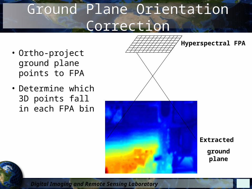
Ground Plane Orientation CorrectionGround Plane Orientation Correction
• Ground plane extraction– Estimated using Lidar last pulse return logic, in combination with
global filtering – Trees and buildings removed using various filtering techniques– Resulting data gaps are filled using interpolation– Leverage technique developed by PhD-candidate Steve Lach
Digital Imaging and Remote Sensing Laboratory
Ground Plane Orientation CorrectionGround Plane Orientation Correction
Hyperspectral FPA
Extracted
ground plane
• Ortho-project ground plane points to FPA
• Determine which 3D points fall in each FPA bin

Digital Imaging and Remote Sensing Laboratory
Ground Plane Orientation CorrectionGround Plane Orientation Correction
• Ortho-project the points associated with ground plane onto the hyperspectral sensor focal plane
• Compute the ground plane normal for each point location using eigenvalue decomposition
• Compute the mean ground plane normal vector for each hyperspectral pixel
• Compute between solar declination vector (i.e. unit vector from sun to global coordinate origin) and mean ground plane normal vector for every pixel
Digital Imaging and Remote Sensing Laboratory
Mixing Fraction PredictionMixing Fraction Prediction
• Challenging problem
• Requires means of recognizing 3D shapes (i.e. targets) in point clouds
• No a priori knowledge of target pose
• Knowledge of sensor location and ground plane does provide a priori knowledge of target scale
• Must be robust in the presence of occlusion

Digital Imaging and Remote Sensing Laboratory
Mixing Fraction PredictionMixing Fraction Prediction
• 3D target matched filter problematic– 6 Degrees of Freedom
• X, y, z, tip, tilt, pan
– Target articulation – Not robust in presence of occlusion
• Spin-Images is potential solution– Adapted technique from Robotic Vision

Digital Imaging and Remote Sensing Laboratory
Spin-ImagesSpin-Images
• 2D parametric space image– Capture 3D shape information about a single point in
3D point cloud– Pose invariant
• Based on local geometry relative to a single point normal• i.e. invariant to tip, tilt, pan
– Scale variant• Estimate scale from ground plane/sensor position
– Graceful detection degradation in the presence of occlusion

Digital Imaging and Remote Sensing Laboratory
Spin-Image FormationSpin-Image Formation
• Step 1: For a given point p in a 3D cloud, estimate point/surface normal– p referred to as spin image basis point– Normal estimate referred to as spin image basis normal– Coordinate space is localized for a single point p– Points are spatial samples of a 3D surface– Define voxel with p at origin– Use eigenvalue decomposition to determine surface
normal– Eigenvector associated with smallest eigenvalue
estimates surface normal

Digital Imaging and Remote Sensing Laboratory
Spin-Image FormationSpin-Image Formation
• Step 2: Calculate 2D parameter space coordinates – Radial distance to
local point normal
– Signed vertical distance along basis normal
22)( pxnpx )( pxn

Digital Imaging and Remote Sensing Laboratory
Spin-Image FormationSpin-Image Formation
• Step 3: Build Spin “Image”– 2D histogram of all points’ alpha and beta
coordinates relative to generation basis point, p
• Spin Image generation variables– Only points within a set range of p are allowed
to contribute to spin image (aka spin support)– Histogram bin size should be ~3-4 times larger
than mean point spacing– Spin angle (described later)

Digital Imaging and Remote Sensing Laboratory
Spin-Image ExamplesSpin-Image Examples
• 3 spin image pairs corresponding to 3 different points on the model
• Left image is high resolution spin image (small bin size)
• Right image is low resolution image (larger bin size) post bilinear interpolation

Digital Imaging and Remote Sensing Laboratory
Spin Image Library MatchingSpin Image Library Matching
• How do I find the model in a real scene?– Build a library of spin images using the model
• Spin image for every point on the model– Note generation variables: spin support, bin size, and spin
angle
• Only has to be done once
– Build a spin image for a point in the scene using same generation variables
– Compare scene spin image to all spin images in model-based library

Digital Imaging and Remote Sensing Laboratory
Spin Image Library MatchingSpin Image Library Matching
• Will a spin image from a target point in my scene match a spin image from the model library?– Model library generated from 3D CAD model
• Points on all sides of model• High sampling density• No occlusion
– Scene• Target and background present• Points only from Lidar illumination direction• Self-occlusion and background occlusion• Not necessarily at same spatial sampling as model library

Digital Imaging and Remote Sensing Laboratory
Spin Image Library MatchingSpin Image Library Matching
• Intelligent model library generation– Typically model has many more points than scene data
• Normalize scene and model spin images
– Scene has points from only one illumination direction• Spin angle limits model points that can contribute to a spin
image when building model library• Compute normal for every point in model• Pick spin image basis point p• Allow only normals within 90° angle relative to spin image
basis normal to contribute to model spin image• This builds self-occlusion effects into model library
Digital Imaging and Remote Sensing Laboratory
Spin Image Library MatchingSpin Image Library Matching
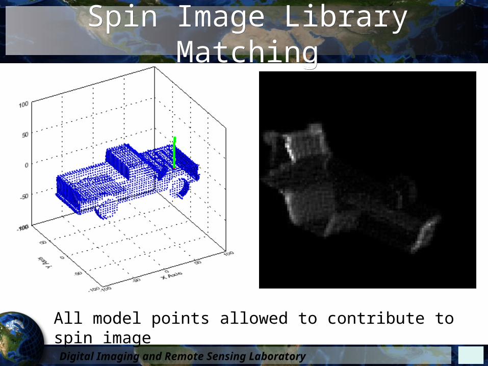
All model points allowed to contribute to spin image

Digital Imaging and Remote Sensing Laboratory
Spin Image Library MatchingSpin Image Library Matching
Only model points (pink) with normals within 85° of spin image basis normal allowed to contribute to spin image

Digital Imaging and Remote Sensing Laboratory
Spin Image Library MatchingSpin Image Library Matching
• Matching with occluded scenes– Compute correlation based on overlapping bins* in the
model spin image and scene spin image– N = number of overlapping bins – Similarity metric, S
– Model library spin image with highest S-score is best match
– Considered a point correspondence between model and scene
S = N × Correlation(Spin*m, Spin*s)

Digital Imaging and Remote Sensing Laboratory
Spin Image Library MatchingSpin Image Library Matching
• Geometric consistency– Ensures similar locations between scene to model
point correspondences– Ensures proper basis normal orientation– Filters out bad correspondences

Digital Imaging and Remote Sensing Laboratory
Spin Image LimitationsSpin Image Limitations
• Need sufficient point density on a surface to accurately estimate normal– May not work for targets under
trees
• Does not adequately address target symmetry– Most common “targets” have a
plane of symmetry– Points symmetric about plane have
identical spin images– May result in bad point
correspondences

Digital Imaging and Remote Sensing Laboratory
Spin Image LimitationsSpin Image Limitations
• Bottom line: spin images may not be a robust target detector for point clouds with low spatial sampling (i.e. most Lidar systems)
• May be good enough to estimate mixing fractions
• Need to quantify mixing fraction uncertainty

Digital Imaging and Remote Sensing Laboratory
Lidar Target DetectionLidar Target Detection
Range-gate scene data
Scene data
Scale 3D CAD Model
Extract ground plane
Create model spin image
library
Select point & create scene spin image
Compare scene spin image to
model spin image library
Sort & filter based on Similarity
Sort & filter Geometric
Consistency
Extract target 3D point locations based on best
model/scene spin images
repeat for n points
Digital Imaging and Remote Sensing Laboratory
Mixing Fraction PredictionMixing Fraction Prediction
• For the best model/scene correspondence– Store spin image bin locations that are non-
zero in both the scene spin image and model spin image (i.e. overlapping bins)
– Extract the 3D point coordinates for the scene points that contributed to the overlapping bins
– Orthoproject 3D target points on to the hyperspectral FPA
– Mixing fraction, M = % of FPA pixel filled by target points

Digital Imaging and Remote Sensing Laboratory
Mixing Fraction PredictionMixing Fraction Prediction
• Final ortho-projection of scene target points onto hyperspectral FPA necessary to estimate mixing fraction M on a per-pixel basis
9.0M
5.0M

Digital Imaging and Remote Sensing Laboratory
Mixing Fraction PredictionMixing Fraction Prediction
• Create M uncertainty bounds – Perform linear unmixing on hyperspectral
image using spectral target vector as an end member
– Requires knowledge of background end members and target spectrum
– Compare unmixing target fraction to M, as predicted from spin image process

Digital Imaging and Remote Sensing Laboratory
AnalysisAnalysis
• Test geometrically-enhanced target detect versus other established methods
• Present results in the form of multiple ROC curves– Compare ROC curves for Rx, Dr. Messinger’s
unconstrained mixed pixel model, traditional physics-based results, and my constrained model
– Compare ROC curves for my model using various degrees of spatial oversampling
– Compare ROC curves for my model for various viewing geometries
• Coincident LIDAR and hyperspectral platforms • Separate platforms with varying pointing geometries

Digital Imaging and Remote Sensing Laboratory
OverviewOverview
• Motivation & Hypothesis
• Methodology– Ground plane orientation correction– Mixing fraction prediction
• Preliminary results

Digital Imaging and Remote Sensing Laboratory
Preliminary ResultsPreliminary Results
• Simulated Lidar point clouds using Rhino
• Fully coded spin image process
• Created high resolution model spin image library
• Created low resolution “scene” point clouds
• Matched scene points to model based on similarity and geometric consistency

Digital Imaging and Remote Sensing Laboratory
Preliminary ResultsPreliminary Results
• Use Rhino to convert facetized model of tank to sampled point cloud – Import obj/3ds model > DrapePt function >
Export point cloud with new vertex locations

Digital Imaging and Remote Sensing Laboratory
Preliminary ResultsPreliminary Results
• Normal estimation via eigenvector decomposition – Select a voxel containing small number of
points– Represent all points in voxel in 2D array (N x 3)
• N rows = point observations• 3 columns = point locations in x, y, z space
– Compute covariance matrix of 2D array– Eigenvector associated with smallest
eigenvalue is estimated normal vector

Digital Imaging and Remote Sensing Laboratory
Spin Image Matching ExamplesSpin Image Matching Examples
• Scene 1 = Model translated, rotated, sampled from off NADIR
VIEW 1Model Scene

Digital Imaging and Remote Sensing Laboratory
Spin Image Matching ExamplesSpin Image Matching Examples
VIEW 2Model Scene
• Scene 1 = Model translated, rotated, sampled from off NADIR

Digital Imaging and Remote Sensing Laboratory
Spin Image Matching ExamplesSpin Image Matching ExamplesScene 1 = Model translated, rotated, sampled from off NADIR
MODEL SPIN IMAGE SCENE 1 SPIN IMAGE

Digital Imaging and Remote Sensing Laboratory
Spin Image Matching ExamplesSpin Image Matching Examples• Scene 2 = Model translated, rotated, sampled from off
NADIR 50% occluded

Digital Imaging and Remote Sensing Laboratory
Spin Image Matching ExamplesSpin Image Matching Examples
Model
• Scene 2 = Model translated, rotated, sampled from off NADIR - 50% occluded + tree clutter
SceneVIEW 1

Digital Imaging and Remote Sensing Laboratory
Spin Image Matching ExamplesSpin Image Matching Examples• Scene 2 = Model translated, rotated, sampled from off
NADIR - 50% occluded + tree clutter
ModelVIEW 2
Scene

Digital Imaging and Remote Sensing Laboratory
Spin Image Matching ExamplesSpin Image Matching Examples
MODEL SPIN IMAGE SCENE 2 SPIN IMAGE
• Scene 2 = Model translated, rotated, sampled from off NADIR - 50% occluded + tree clutter

Digital Imaging and Remote Sensing Laboratory
ConclusionsConclusions
• Constraining the target space associated with physics-based modeling may improve target detection performance
• 3D spatial information from Lidar may provide a means of estimating geometric parameter bounds
• Target detection based on fused spectral and spatial information may prove to be more robust than each sensing modality alone

Digital Imaging and Remote Sensing Laboratory

Digital Imaging and Remote Sensing Laboratory

Digital Imaging and Remote Sensing Laboratory
Spin Image Surface MatchingSpin Image Surface Matching

Digital Imaging and Remote Sensing Laboratory
Model / Scene RegistrationModel / Scene Registration
• Pink points represent occluded scene points of the bunny• Green 3D model of the bunny has been registered to
scene points

Digital Imaging and Remote Sensing Laboratory
A
B
C
Sensor-reaching Radiance PathsSensor-reaching Radiance Paths

Digital Imaging and Remote Sensing Laboratory
Mixing FractionsMixing Fractions
25.0M
1M