1

Geometric camera calibration using circular control points

Janne HeikkiläMachine Vision and Media Processing Unit

Infotech Oulu and Department of Electrical EngineeringFIN-90014 University of Oulu, Oulu, Finland

jth@ee.oulu.fi

Abstract

Modern CCD cameras are usually capable of a spatial accuracy greater than 1/50 of the pixel

size. However, such accuracy is not easily attained due to various error sources that can affect

the image formation process. Current calibration methods typically assume that the observa-

tions are unbiased, the only error is the zero-mean independent and identically distributed ran-

dom noise in the observed image coordinates, and the camera model completely explains the

mapping between the 3-D coordinates and the image coordinates. In general, these conditions

are not met, causing the calibration results to be less accurate than expected. In this paper, a cal-

ibration procedure for precise 3-D computer vision applications is described. It introduces bias

correction for circular control points and a non-recursive method for reversing the distortion

model. The accuracy analysis is presented and the error sources that can reduce the theoretical

accuracy are discussed. The tests with synthetic images indicate improvements in the calibra-

tion results in limited error conditions. In real images, the suppression of external error sources

becomes a prerequisite for successful calibration.

Keywords: camera model, lens distortion, reverse distortion model, calibration procedure, bias

correction, calibration accuracy

1 Intr oduction

In 3-D machine vision, it necessary to know the relationship between the 3-D object coordinates

and the image coordinates. This transformation is determined in geometric camera calibration

by solving the unknown parameters of the camera model. Initially, camera calibration tech-

niques were developed in the field of photogrammetry for aerial imaging and surveying. First,

2

photographic cameras were used, but recently video cameras have replaced them almost com-

pletely. Also new application areas, like robot vision and industrial metrology, have appeared,

where camera calibration plays an important role.

Depending on the application, there are different requirements for camera calibration. In

some applications, such as robot guidance, the calibration procedure should be fast and auto-

matic, but in metrology applications, the precision is typically a more important factor. The tra-

ditional camera calibration procedures such as bundle adjustment [1] are computationally

greedy full scale optimization approaches. Therefore, most of the calibration methods suggested

during the last few decades in computer vision literature are mainly designed for speeding up

the process by simplifying or linearizing the optimization problem. The well known calibration

method developed by Roger Tsai [2] belongs to this category. Also other techniques based on

the linear transformation, for example [3, 4, 5, 6], are fast but quite inaccurate. The simplifica-

tions made reduce the precision of the parameter estimates, and as a consequence, they are not

suitable for applications in 3-D metrology as such.

Due to the increased processing power of standard workstations, the nonlinear nature of the

estimation problem is not as restricting as it was a few years ago. The calibration procedure can

be accomplished in a couple of seconds iteratively. This gives us a good reason for improving

the accuracy of the calibration methods without introducing a lot of extra time for computation.

An accuracy of 1/50 of the pixel size (around 1/50,000 of the image size) is a realistic goal that

can be achieved in low noise conditions with proper subpixel feature extraction techniques. The

main improvements in the new calibration procedure presented in the following sections are the

camera model, which allows accurate mapping in both directions, and the elimination of the bias

in the coordinates of the circular control points.

In Section 2, we begin by describing the camera model for projection and back-projection.

In Section 3, the projective geometry of the circular control points is reviewed and the necessary

equations for mapping the circles into the image plane are presented. Section 4 describes a

three-step calibration procedure for circular control points. Experimental results with the cali-

3

bration procedure are reported in Section 5, and the effects of some typical error sources are dis-

cussed in Section 6. Finally, Section 7 offers concluding remarks.

2 Camera model

In camera calibration, the transformation from 3-D world coordinates to 2-D image coordinates

is determined by solving the unknown parameters of the camera model. Depending on the ac-

curacy requirements the model is typically based on either orthographic or perspective projec-

tion. Orthographic transformation is the roughest approximation assuming the objects in 3-D

space to be orthogonally projected on the image plane. It is more suitable for vision applications

where the requirements of the geometric accuracy are somewhat low. Due to linearity, it pro-

vides a simpler and computationally less expensive solution than perspective projection which

is a nonlinear form of mapping. However, for 3-D motion estimation and reconstruction prob-

lems, perspective projection gives an idealized mathematical framework, which is actually quite

accurate for high quality camera systems. For off-the-shelf systems, the perspective projection

model is often augmented with a lens distortion model.

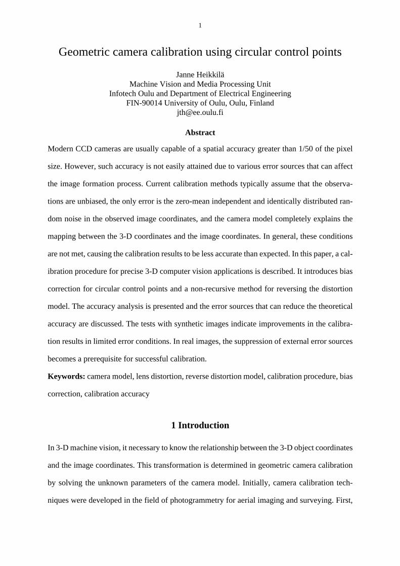
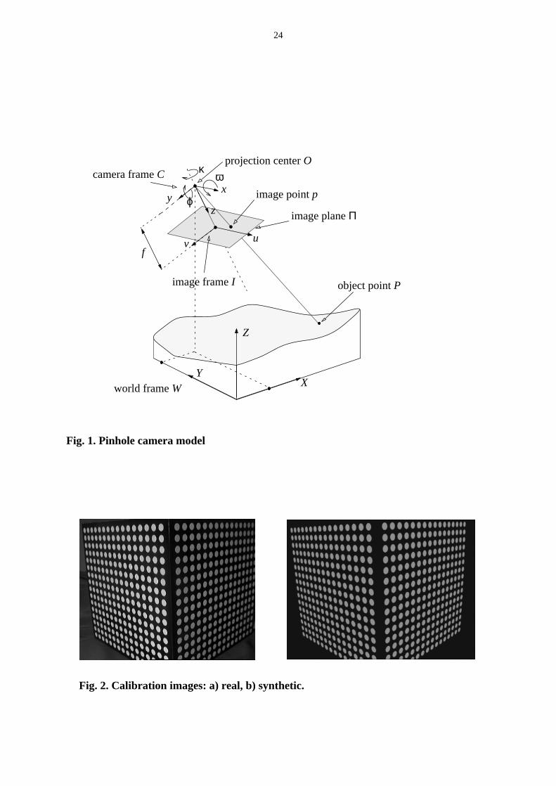
Let us first consider a pure perspective projection (i.e. pinhole) camera model illustrated in

Fig. 1. The center of projection is at the originO of the camera frameC. The image planeΠ is

parallel to thexy plane and it is displaced with a distancef (focal length) fromO along thez axis.

Thez axis is also called the optical axis, or the principal axis, and the intersection ofΠ and the

optical axis is called the principal pointo. Theu andv axes of the 2-D image coordinate frame

I are parallel to thex andy axes, respectively. The coordinates of the principal point inI are [u0,

v0]T.

Let P be an arbitrary 3-D point located on the positive side of thez axis andp its projection

on Π. The coordinates ofP in the camera frameC are [x, y, z]T, and in the world frameW the

4

coordinates are [X, Y, Z]T. The coordinates ofp in I are [u, v]T and they can be solved from the

homogeneous coordinates given by the transformation

whereF is the perspective transformation matrix (PTM),

λ is a scale factor,s is the aspect ratio, andM is a 4 by 4 matrix describing the mapping from

W to C. It is decomposed as follows:

wheret = [tx, ty, tz]T describes the translation between the two frames, andR is a 3 by 3 or-

thonormal rotation matrix which can be defined by the three Euler anglesω, ϕ, andκ. If R is

known, these angles can be computed using, for example, the following decomposition [6]:

wherer ij is the entry from theith row and thejth column of the matrixR, and atan2(y, x) is the

two-argument inverse tangent function giving the angle in the range (-π, π]. Because

the Euler angles do not represent the rotation matrix uniquely. Hence, there

are two equivalent decompositions for the matrixR. As we can see, Eqn (4) has singularity if

, i.e., or . In those cases, we can chooseκ = 0, and

, or vice versa [6]. In most situations, we could also prevent the singular-

ities by carefully planning the calibration setup.

(1)u

v

1

λu

λv

λ

∝ F

X

Y

Z

1

PM

X

Y

Z

1

= =

(2)Psf 0 u0 0

0 f v0 0

0 0 1 0

,=

(3)M R t0 1

=

(4)

ϕ sin1–r31=

ω 2r32

ϕcos------------–

r33

ϕcos------------,

atan=

κ 2r21

ϕcos------------–

r11

ϕcos------------,

atan=

ϕsin π ϕ–( )sin=

r31 1±= ϕ π 2⁄= ϕ 3π 2⁄=

ω 2 r12 r22,( )atan=

5

The parameterstx, ty, tz, ω, ϕ, andκ are calledextrinsic parameters or exterior projective

parameters and the parameterss, f, u0 andv0 are theintrinsic parameters or interior projective

parameters of the pinhole camera model.

It is usually more convenient to express the image coordinates in pixels. Therefore the co-

ordinates obtained from Eqn (1) are multiplied by factorsDu andDv that specify the relationship

between pixels and the physical object units, for example, millimeters. However, knowing the

precise values of these conversion factors is not necessary because they are linearly dependent

on the parameterss andf that are adjusted during calibration.

In real cameras, perspective projection is typically not sufficient for modeling the mapping

precisely. Ideally, the light rays coming from the scene should pass through the optical center

linearly, but in practice, lens systems are composed of several optical elements introducing non-

linear distortion to the optical paths and the resulting images. The camera model of Eqn (1) pro-

duces the ideal image coordinates [u, v]T of the projected pointp. In order to separate these

errorless but unobservable coordinates from their observable distorted counterparts we will

henceforth denote the correct or corrected coordinates of Eqn (1) byac = [uc, vc]T and the dis-

torted coordinates byad = [ud, vd]T.

Several methods for correcting the lens distortion have been developed. The most common-

ly used approach is to decompose the distortion into radial and decentering components [7].

Knowing the distorted image coordinatesad, the corrected coordinatesac are approximated by

where

, , , and . The parame-

tersk1, k2,... are the coefficients for the radial distortion that causes the actual image point to be

displaced radially in the image plane, and the parametersp1, p2,... are the coefficients for the

(5)ac ad�

D ad δ,( )+=

(6)�

D ad δ,( )ud k1rd

2k2rd

4k3rd

6 …+ + +( ) 2p1udvd p2 rd2

2ud2

+( )+( ) 1 p3rd2 …+ +( )+

vd k1rd2

k2rd4

k3rd6 …+ + +( ) p1 rd

22vd

2+( ) 2p2udvd+( ) 1 p3rd

2 …+ +( )+=

ud ud u0–= vd vd v0–= rd ud2

vd2

+= δ k1 k2 … p1 p2 …, , , , ,[ ]T=

6

decentering or tangential distortion which may occur when the centers of the curvature of the

lens surfaces in the lens system are not strictly collinear.

Other distortion models have also been proposed in the literature. For example, Melen [6]

used a model whereP in Eqn (2) was augmented with terms for linear distortion. This is useful

if the image axes are not orthogonal, but in most cases the CCD arrays are almost perfect rect-

angles, and hence the linear distortion component is insignificant (less than 0.01 pixels [8]). In

the calibration method proposed by Faugeras and Toscani [5], the geometric distortion was cor-

rected using bilinear transformation in small image regions.

For camera calibration, it is favorable to find a transformation from the 3-D world coordi-

nates to the real image coordinates. This enables us to use a least squares technique as an opti-

mal estimator of the camera parameters. Directly applying Eqns (1) and (5) implies that we first

need to correct the distortion and then estimate the camera parameters of Eqn (1). An obvious

problem is that the distortion coefficients are not usually known in advance, and due to strong

coupling they cannot be reliably estimated without knowing the other camera parameters.

In the literature, there are several solutions to overcome this problem. Tsai [2] and Lenz and

Tsai [9] decomposed the camera model into linear and nonlinear parts where the parameters are

decoupled. However, only radial distortion can be used, and the solution is not optimal. Weng

et al. [10] suggested an iterative scheme where the parameters of the distortion model and the

projection model are fixed in turn, and estimated separately. A commonly used approach in pho-

togrammetry [7] is to perform a full scale optimization for all parameters by minimizing the sum

of squared errors between the corrected image coordinates and the synthetic coordinates given

by the camera model. In practice, this means that Eqn (6) is evaluated with noisy observations,

which may deteriorate the calibration result. In order to minimize the error between the ob-

served and model coordinates, the distorted image coordinates should be expressed in terms of

their undistorted counterparts. For this we need an inverse distortion model. As can be easily

7

noticed, there is no analytic solution for the inverse problem, and thus, we need to approximate

it. Melen [6], for example, used the following model:

The fitting results given by this model are often satisfactory, because the distortion coefficients

are typically small values causing the model to be almost linear. It should be noticed that the

optimal distortion coefficients in a least squares sense are different for Eqns (5) and (7).

Another solution is to create the following recursion based on Eqn (5):

The error introduced when substituting with on the right-hand side gets smaller for each

iteration. In practice, at least three or four iterations are required to compensate for strong lens

distortions. This means that the distortion function is evaluated several times in different

locations of the image, which makes this technique less attractive.

In order to avoid extensive computation, we can take a first order Taylor series approxima-

tion of about :

where

Solving from Eqn (9) yields

The elements ofD(ac) are small (<< 1) which makes it possible to use the following approxi-

mation:

(7)ad ac�

D ac δ,( )–≈

(8)ad ac

�D ad δ,( )– ac

�D ac

�D ad δ,( )– δ,( )–≈ ≈

ac�

D ac�

D ac�

D ad δ,( )– δ,( )– δ,( )– …≈ ≈

ad ac

�D

�D ac( ) ac

(9)ac ad�

D ac δ,( ) D ac( ) ad ac–( )+ +≈

(10)D ac( )u∂

∂ �

D a δ,( )v∂

∂ �

D a δ,( )a ac=

=

ad

(11)ad ac I D ac( )+( ) 1– �

D ac δ,( )–≈

8

whered11(ac) andd22(ac) are the upper left and lower right elements ofD(ac), respectively. If

only two radial distortion coefficientsk1 andk2, and two decentering distortion coefficientsp1

andp2 are used, the approximation of the inverse distortion model becomes

where . If necessary, extending this model with higher order terms is straightfor-

ward.

By replacingu = uc andv = vc in Eqn (1) and combining it with Eqn (12), we obtain afor-

ward camera model which converts the 3-D world coordinates to distorted image coordinates.

Using abackward camera model, we can transform the distorted camera coordinates to

lines of sight in the 3-D world coordinate system, or to the intersections of these lines with a

known 2-D plane. Let us assume that we have a 2-D planeΠ’ with a coordinate systemH,

whose origin is ath0 = [X0, Y0, Z0]T, and it is spanned by the 3-D vectorsh1 = [X1, Y1, Z1]

T and

h2 = [X2, Y2, Z2]T. The transformation from the corrected image coordinatesac = [uc, vc]

T pro-

duced by Eqn (5) on the planeΠ’ can be expressed as

whereλ is a scale factor,xH = [XH, YH]T are the back projected coordinates inH and

Due to the approximations made, is not the exact inverse function of . Therefore it

may be necessary to use different parametersδ’ in Eqn (6) than in Eqn (13). A method for esti-

mating these parameters will be presented in Section 4.

(12)ad ac1

d11 ac( ) d22 ac( ) 1+ +----------------------------------------------------

�D ac δ,( )– ac

�D* ac δ,( )–≡≈

(13)�

D* ac δ,( ) 1

4k1r c2

6k2r c4

8p1vc 8p2uc 1+ + + +-------------------------------------------------------------------------------------

�

D ac δ,( )=

r c uc2

vc2

+=

(14)λ xH

1FH( ) 1– ac

1=

Hh1 h2 h0

0 0 1=

�

D* �

D

9

3 Circular control points

Lines in the object space are mapped as lines on the image plane, but in general perspective pro-

jection is not a shape preserving transformation. Two- and three-dimensional shapes are de-

formed if they are not coplanar with the image plane. This is also true for circular landmarks,

which are commonly used control points in calibration. However, a bias between the observa-

tions and the model is induced if the centers of their projections in the image are treated as pro-

jections of the circle centers. In this section, we will review the necessary equations for using

the centers of the projections as image observations without introducing any bias.

Let us assume that a circular control pointR with radiusr is located on the planeΠ’so that

its center is at the origin of the planar coordinate frameH. Circles are quadratic curves that can

be expressed in the following manner:

whereA, B, C, D, E andF are coefficients that define the shape and location of the curve. In

homogeneous coordinates, this curve can be written as

where

For the circleR

Using Eqn (14),R can be projected on the image plane. The resulting curve becomes

(15)AXH2

2BXHYH CYH2

2DXH 2EYH F+ + + + + 0=

(16)xH

1

T

QxH

10=

QA B D

B C E

D E F

=

Q1 r

2⁄– 0 0

0 1 r2⁄– 0

0 0 1

=

10

where

We can see that the result is a quadratic curve, whose geometric interpretation is a circle, hy-

perbola, parabola, or ellipse. In practice, due to the finite rectangle corresponding to the image

plane, the projection will be an ellipse, or in some special cases, a circle. As shown in [11], the

center of the ellipseec = [ue, ve]T can be obtained from

By combining Eqns (18) and (19) we get

where , andf3 is a vector consisting of the last row ofF. The matrixG specifies

the geometry, position, and orientation of the control point, and the perspective transformation

matrix F specifies the mapping from the world coordinates to undistorted image coordinates

that can be further converted to distorted image coordinatesed using Eqn (12). As a result, we

get

It should be noticed that using Eqn (20) instead of Eqn (1), we obtain an unbiased relation-

ship between the observed centers of the ellipses and the camera model.

4 Calibration pr ocedure

The calibration procedure presented next is mainly intended to be used with circular landmarks.

However, it is also suitable for small points without any specific geometry. In that case, the ra-

(17)ac

1

T

Sac

10=

(18)S FH( ) 1–( )TQ FH( ) 1–

=

(19)λ ec

1S 1–

0

0

1

=

(20)λ ec

1FGf 3=

G HQ 1– HT=

(21)ed ec�

D* ec δ,( )–=

11

dius is set to zero. It is assumed that the camera model includes eight intrinsic parametersθint

= [s, f, u0, v0, k1, k2, p1, p2]T and six extrinsic parametersθext = [tx, ty, tz, ω, ϕ, κ]T. If necessary,

adding higher order terms to the model is straightforward. In multi-frame calibration, each

frame has separate extrinsic parameters, but common intrinsic parameters. The radius of control

pointsr and the conversion factorsDu andDv are assumed to be known in advance, as well as

the 3-D coordinates, and the observed image coordinates of the control points.

Due to the nonlinear mapping of the camera model, there are no direct estimators of all the

camera parameters that would produce an optimal solution in a least squares sense. We there-

fore use an iterative searching technique to estimate the vector

whereK is the number of the frames. Before using the estimator, we need to have initial values

of the camera parameters for guaranteeing that a global minimum can be achieved. This prob-

lem is solved by ignoring the lens distortion and using a linear estimator for the rest of the pa-

rameters.

Step 1: Initialization

Many variations of the linear calibration technique have been proposed in the literature, for ex-

ample [3, 4, 5, 6]. However, they are all based on the same idea where the perspective transfor-

mation matrixF is first estimated and then decomposed into intrinsic and extrinsic camera

parameters. These methods provide a closed-form solution to the camera parameters. The major

shortcoming is that they are not optimal estimators, because they do not produce minimum vari-

ance estimates. Another problem is that they ignore the effects of the radial and decentering lens

distortion. Despite these shortcomings linear calibration techniques can provide a good starting

point for iterative search.

Several well known procedures for estimatingF are available, e.g. [5]. The main difference

between the linear calibration methods is that howF is decomposed into camera parameters.

(22)θT θint

T θextT

1( ) θextT

2( ) … θextT

K( ), , , ,[ ]=

12

For example, Faugeras and Toscani [5] extracted five intrinsic and six extrinsic parameters us-

ing a set of linear equations, and Melen [6] used QR decomposition for estimating six intrinsic

and six extrinsic parameters. In principle, these techniques can be directly applied to obtain the

initial estimate for the iterative optimization step. However, due to the shortcomings listed

above these estimators tend to be rather sensitive to observation noise. Even small inaccuracy

in F can cause significant errors especially in the intrinsic parameters. As a consequence, opti-

mization may fail.

In the initialization step, where the aim is to produce the first, not the final, estimates of the

camera parameters, it is often more reliable to use the nominal values for the focal length, the

aspect ratio and the image center as the intrinsic parameters. With these values, we can directly

write the projection matrixP using Eqn (2). Let us assume that the control points are not copla-

nar, which means that we have a full 3 by 4 estimate of the perspective transformation matrixF

denoted by . Thus, we can write the following equation:

whereP13 is a matrix containing the first three columns ofP, and are the estimates ofR

andt, respectively. Now, it is straightforward to get

and

where is a matrix containing the first three columns, and the last column of .

The matrix does not satisfy the orthonormality constraint of a standard rotation matrix,

but we can normalize and orthogonalize it using the singular value decomposition (SVD):

The orthonormal version of is given by

F̂

(23)F̂ PM̂ P13R̂ P13t̂= =

R̂ t̂

(24)R̂ P131– F̂13=

(25)t̂ P131– F̂4=

F̂13 F̂4 F̂

R̂

(26)R̂ UΣVT

=

R̂

(27)R'ˆ UΣ'VT=

13

where is a diagonal matrix with diagonal elements 1, 1, and in descending order [11].

The Euler angles can now be extracted from using Eqn (4).

If all the control points are coplanar, only a submatrix ofF can be determined. Basically,

the procedure is the same as above, with the exception that only two columns of are estimat-

ed. The third column is easily obtained by utilizing the orthogonality of the basis vectors. If

multi-frame calibration is used, the initialization step is performed separately for every frame.

The initial parameters are collected into a vector

wheref0 is the nominal focal length,Nu andNv are the horizontal and vertical dimensions of the

image.

Step 2: Iterative search

In this step, the parameters of the forward camera model are estimated by minimizing the

weighted sum of squared differences between the observations and the model. Let us assume,

that there areN circular control points andK images that are indexed byn = 1,...,N andk = 1,...,

K. A vector containing the observed image coordinates of the center of the ellipsen in the frame

k is denoted by , and the corresponding vector produced by the forward camera model

of Eqns (20) - (21) is denoted by . Now, the objective function can be expressed as

where

andR is the covariance matrix of the observation error. There are various sources that can affect

R. Some of them are discussed later, in Section 6. If the covariance matrix is unknown or the

measurement noise for individual observations is statistically independent and identically dis-

tributed,R-1 in Eqn (29) can be omitted. In general, the assumption of the statistically indepen-

dent and identically distributed noise is not fulfilled, because the error variance depends on the

size of the ellipse in the image, and the covariance between the horizontal and vertical coordi-

Σ' UVT

R'ˆ

R'ˆ

(28)θ̂0T

1 f 0 Nu 2⁄ Nv 2⁄ 0 0 0 0 θextT

1( ) θextT

2( ) … θextT

K( ), , , , , , , , , , ,[ ]=

eo n k,( )

ed n k,( )

(29)J θ( ) yT θ( )R 1– y θ( )=

yT θ( ) eo 1 1,( ) ed 1 1,( )–( )T eo 2 1,( ) ed 2 1,( )–( )T … eo N K,( ) ed N K,( )–( )T, , ,[ ]=

14

nates is non-zero if the ellipse is inclined. As a consequence, the measurement noise covariance

matrixR can be expressed as

where

If R(n, k) is not known, it can be estimated. In practice, this means that we need to take several

images from the same position and orientation, and then calculate the sample covariance in the

following manner:

whereW is the number of the images used for estimatingR(n, k), is the observed

image coordinates (ellipsen, posek, framei), and is the vector of the average coordi-

nates. An obvious problem of this approach is that a large number of images needs to be taken

for single calibration.

The parameters of the forward camera model are obtained by minimizingJ(θ):

There are several numerical techniques, such as the Levenberg-Marquardt method [12], that can

be applied for the optimization problem of Eqn (32). With an efficient technique, only a few

iterations are typically needed to attain the minimum.

Step 3: Backward camera model

In many applications, the observed image coordinates need to be projected back to 3-D coordi-

nates. This procedure was already described in Section 2. However, the reverse distortion model

of Eqn (13), used in Step 2, is not exactly the inverse of Eqn (6). In order get more consistent

(30)R

R 1 1,( ) 0 … 00 R 2 1,( ) … 0... ... … ...

0 0 … R N K,( )

=

R n k,( ) E eo n k,( ) E eo n k,( ){ }–[ ] eo n k,( ) E eo n k,( ){ }–[ ]T{ }=

(31)R̂ n k,( ) 1W 1–-------------- eo n k i, ,( ) eo n k,( )–[ ] eo n k i, ,( ) eo n k,( )–[ ]

T

i 1=

W

∑=

eo n k i, ,( )

eo n k,( )

(32)θ̂ min Jθ

θ( )arg=

15

results in both directions, we estimate the parameter vector of

Eqn (6) separately. The other intrinsic parameters are the same for both forward and backward

models.

If the steps 1 and 2 have been completed, the parameters of the forward model are already

available. Using this model we can produce a set of distorted points {ad(i)} for arbitrary points

{ ac(i)}, wherei = 1,...,M. The points {ac(i)} are generated so that they form an equally spaced

2-D grid of about 1000 - 2000 points, for example 40 by 40. Points must cover the entire image

area and the outermost points should be approximately 5% - 10% outside the effective image

region in order to get accurate mapping also close to the image borders. If the inversion were

exact, these points would fulfill Eqn (5) expressed in the following matrix form:

where

, , and . Due to the approxima-

tions made in derivation of the inverse distortion model, Eqn (33) does not hold exactly. There-

fore we need to adjust the parameter vectorδ for back projection. This can be performed using

the following least squares formulation:

where is the vector of the distortion parameters to be used in the backward camera model,

and [. ]+ denotes the pseudoinverse of the matrix [13].

δ k1 k2 … p1 p2 …, , , , ,[ ]T=

(33)

ac 1( ) ad 1( )–

ac 2( ) ad 2( )–

:̇

ac M( ) ad M( )–

B 1( )B 2( )

:̇

B M( )

δ=

B i( )ud i( )rd

2i( ) ud i( )rd

4i( ) … 2ud i( )vd i( ) rd

2i( ) 2ud

2i( )+ …

vd i( )rd2

i( ) vd i( )rd4

i( ) … rd2

i( ) 2vd2

i( )+ 2ud i( )vd i( ) …=

ud i( ) ud i( ) u0–= vd i( ) vd i( ) v0–= rd i( ) ud2

i( ) vd2

i( )+=

(34)δ'ˆ

B 1( )B 2( )

:̇

B M( )

+ ac 1( ) ad 1( )–

ac 2( ) ad 2( )–

:̇

ac M( ) ad M( )–

=

δ'ˆ

16

5 Experiments

The camera calibration procedure suggested in Section 4 was tested in two experiments. Firstly,

the parameter estimates of the forward camera model were analyzed statistically using synthetic

images and the results were compared with the outcome of a corresponding real image. Second-

ly, the precision of the inverse distortion model of Eqn (13) was evaluated by correcting and

distorting random image coordinates.

5.1 Calibrating the forward camera model

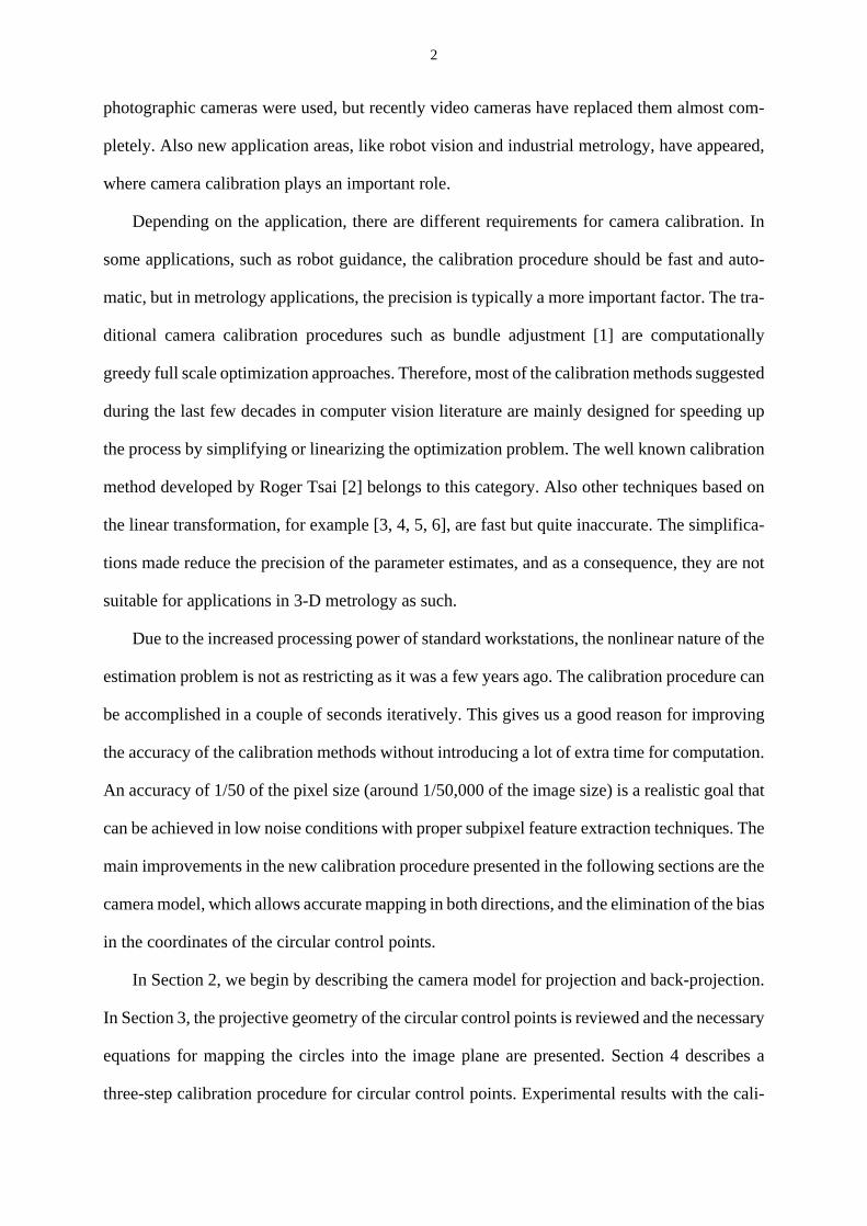
The tests were performed with 200 synthetic images and one real image that was used as a ref-

erence model. This real image shown in Fig. 2a was captured using an off-the-shelf mono-

chrome CCD camera (Sony SSC-M370CE) equipped with a 6.3 mm by 4.7 mm image sensor

and an 8.5 mm Cosmicar TV lens. The image was digitized from an analog CCIR type video

signal using a Sunvideo frame grabber. The size of the image is 768 by 576 pixels, and the max-

imum dynamics is 256 gray levels. In the image, there is a calibration object which has two per-

pendicular planes, each with 256 circular control points. The centers of these points were

located using the moment and curvature preserving ellipse detection technique [14] and renor-

malization conic fitting [15]. The calibration procedure was first applied to estimate the camera

parameters based on the real image. The synthetic images were then produced using ray tracing

with the camera parameters obtained from calibration and the known 3-D model of the control

points. In order to make the synthetic images better correspond to the real images, their intensity

values were perturbed with additive Gaussian noise (σ = 2), and blurred using a 3 by 3 Gaussian

filter (σ = 1 pixel). A sample image is shown in Fig. 2b.

With the synthetic images, we restrict the error sources only to quantization and random im-

age noise. Ignoring all the other error sources is slightly unrealistic, but in order to achieve ex-

tremely accurate calibration results, these error sources should be eliminated or at least

minimized somehow. The advantage of using simulated images instead of real images is that

we can estimate some statistical properties of the procedure.

17

The control points from the synthetic images were extracted using the same techniques as

with the real image, i.e., subpixel edge detection and ellipse fitting. Three different calibration

methods were applied separately for all point sets. The first method (method A) is the traditional

camera calibration approach which does not assume any geometry for the control points. In the

second method (method B), circular geometry is utilized and all the observations are equally

weighted. In the third method (method C), each observation is weighted by the inverse of the

observation error covariance matrixR that was estimated using Eqn (31) and all 200 images.

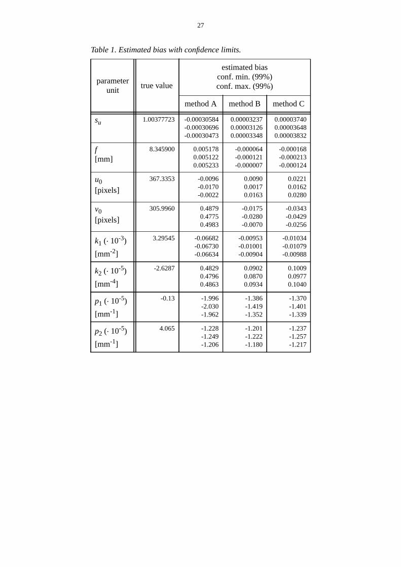
Table 1 shows the estimated bias (average error) of the intrinsic parameters for all three meth-

ods. Confidence intervals with a 95% confidence level are also presented. As we can notice, all

three methods produced slightly biased estimates. However, by regarding the circular geometry

of the control points we can reduce the bias significantly. The remaining error is caused by the

subpixel ellipse detector which is not completely unbiased. However, the effect of the remain-

ing error is so small that it does not have any practical significance.

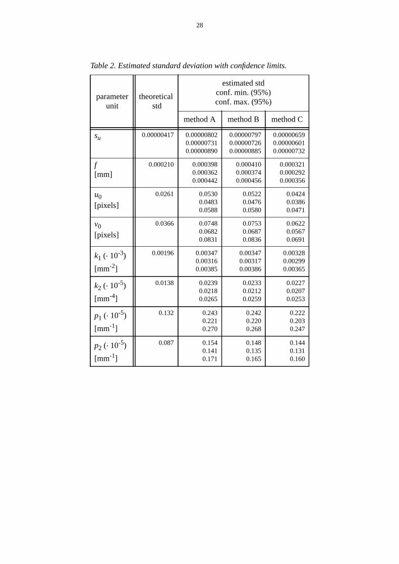
The estimated standard deviation of the intrinsic parameters are given in Table 2. The the-

oretical accuracy that can be attained is approximated using the following equation:

where is the Jacobian matrix ofy(θ) evaluated in . The sameR is used as in the calibra-

tion method C. Now, we can see that the results provided by the methods A and B do not differ

significantly in standard deviation, but in method C, where individual weighting values were

used, the precision is much better. For all methods the theoretical value is still quite far. The

main reason for this is that the covariance matrixR was not known precisely in advance, and it

had to be estimated first. As a result, the camera parameters are not optimal, and on the other

hand,R also became under-estimated in this case, causing the theoretical values to be clearly

smaller than their true values.

Computationally, the new procedure does not increase the number of the iterations required.

For methods A and B, eleven iterations were performed on average. For method C, around 20

iterations were needed in order to achieved convergence. For methods B and C, where the cir-

(35)C E θ θ̂–( ) θ θ̂–( )T

[ ] L T θ̂( )R 1– L θ̂( )[ ]1–

≈=

L θ̂( ) θ̂

18

cular geometry is regarded, the average fitting residual for the synthetic images was around 0.01

pixels, which is better than the original requirement of 1/50 pixels. For method A, the error is

over 0.02 pixels which exceeds the limit.

In reality, the error sources that are not considered in the previous simulations can increase

the residual significantly. For example, using the real image shown in Fig. 2a the average resid-

ual error is 0.048 pixels (horizontal) and 0.038 pixels (vertical) which is a sign of the small error

components originating from the camera electronics, illumination, optical system and calibra-

tion target. Obviously, the accuracy of the calibration result for real images is strongly coupled

with these error sources.

5.2 Calibrating the reverse distortion model

In this experiment, the accuracy of the reverse distortion model was tested with a wide range of

the distortion parameters. The third step of the calibration procedure was applied to solve the

parameter vector for eachδ. Next, 10,000 random points were generated inside the image

region. These simulated points were then corrected using Eqn (5) and distorted again using Eqn

(12). The difference between the resulting coordinates and the original coordinates was exam-

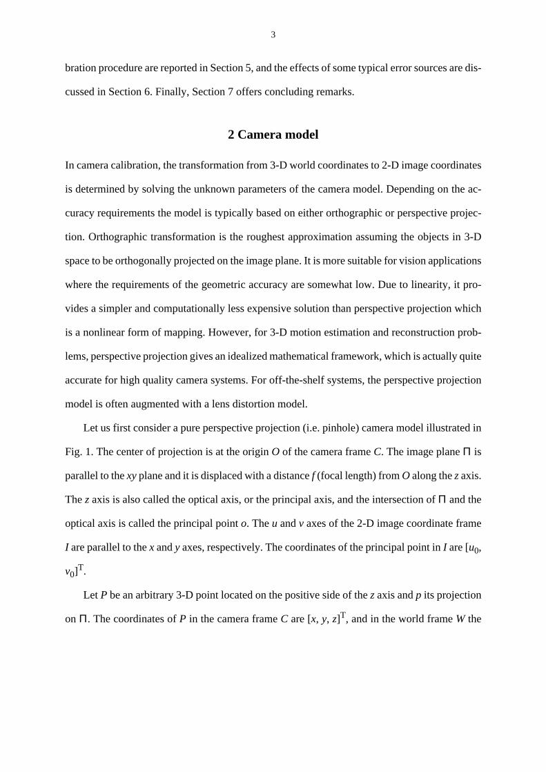
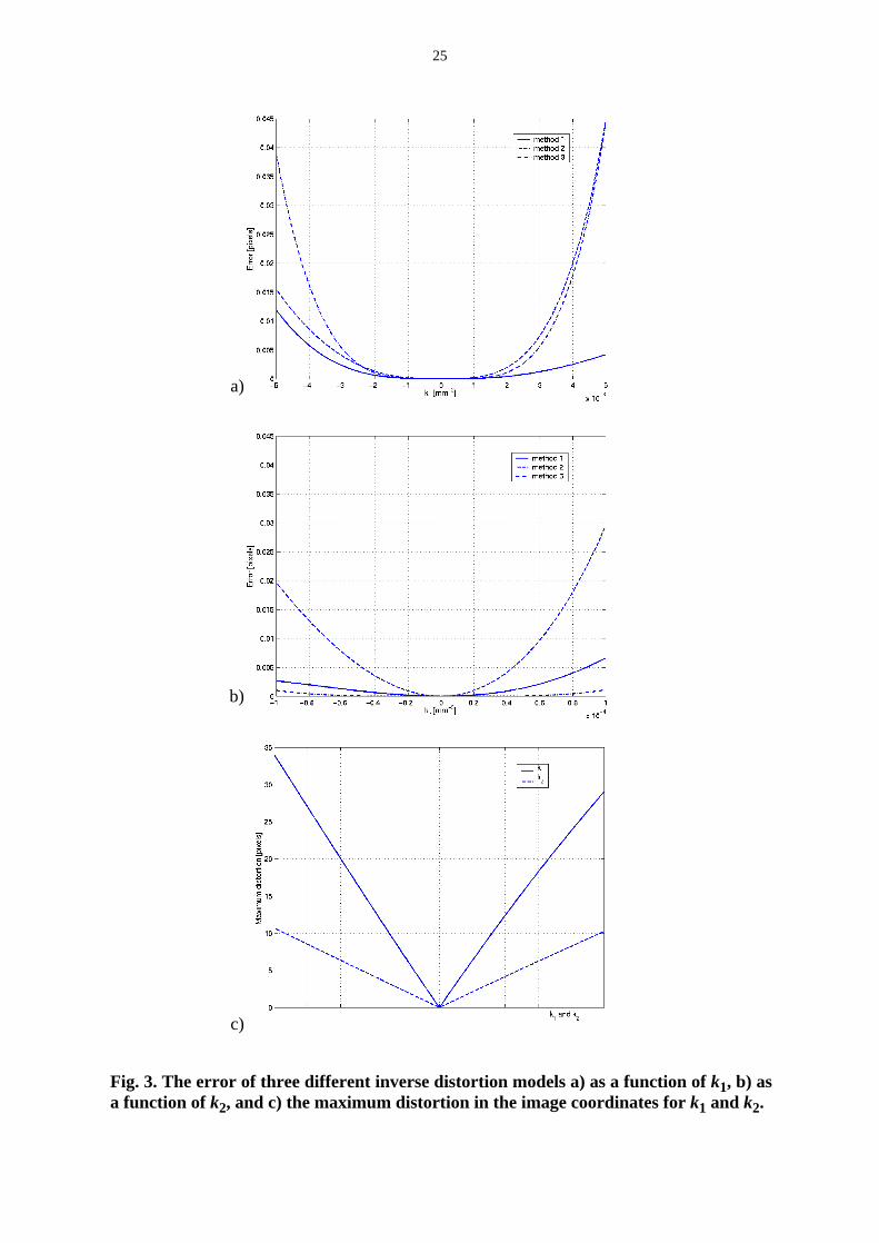
ined with respect to the different values of the distortion parameters. The solid curve in Fig. 3a

represents the root mean square error in the image coordinates as a function of the first radial

distortion parameterk1. The range of the parameter should cover most of the commonly used

off-the-shelf lenses. It can be seen that the error remains below 0.005 pixels for almost all pa-

rameter values. As a reference, results given by two other techniques have also been presented.

Method 2 is based on the idea of using the distortion model in a reverse direction, as given by

Eqn (7) with the exception of estimating the parameter values separately for both directions in

order to improve the result. Method 3 is a recursive approach, and it is based on Eqn (8) with

three iterations. Both of these two methods clearly result in a significantly larger error than

method 1.

In Fig. 3b the same test was performed with the second radial distortion coefficientk2. Now,

δ'ˆ

19

method 3 seems to outperform method 1, but in both cases the error remains small. Method 2 is

clearly the most inaccurate, causing errors that can be significant in precision applications. Fig.

3c shows the maximum radial distortion for both of the two parameters. The first parameter is

typically dominating and the effect of the second parameter is much smaller. For some lenses,

using the third radial distortion coefficient can be useful, but still its effect remains clearly be-

low the other two parameters. The same test procedure was also performed with decentering

distortion, but the error after correcting and distorting the points was noticed to be insignificant-

ly small for all three methods.

6 Other calibration errors

The synthetic images used in the previous section were only subject to quantization noise and

random Gaussian noise. As noticed with the real image, there are also other sources that may

deteriorate the performance of the calibration procedure. In this section, we will briefly review

some of the more significant error sources.

Insufficient projection model: Although the distortion model of Eqn (6) is derived using exact

ray tracing, there can still exist distortion components, especially in wide angle optics that are

not compensated for by this model. The camera model used assumes that the principal point co-

incides with the center of distortion. As stated in [16], this assumption is not eligible for real

lens systems. Furthermore, in the pinhole camera model, the rays coming from different direc-

tions and distances go through a single point, i.e. the projection center. This is a good approxi-

mation for most of the applications, but unfortunately real optics do not behave exactly like that.

There is usually some nonlinear dependence between the focal length, imaging distance and the

size of the aperture. As a consequence, for apertures larger than a pinhole the focal length is

slightly changing, especially in short distances.

Illumination changes: Changes in the irradiance and the wavelength perceived by the camera

are typically neglected in geometric camera calibration. However, variation in lighting condi-

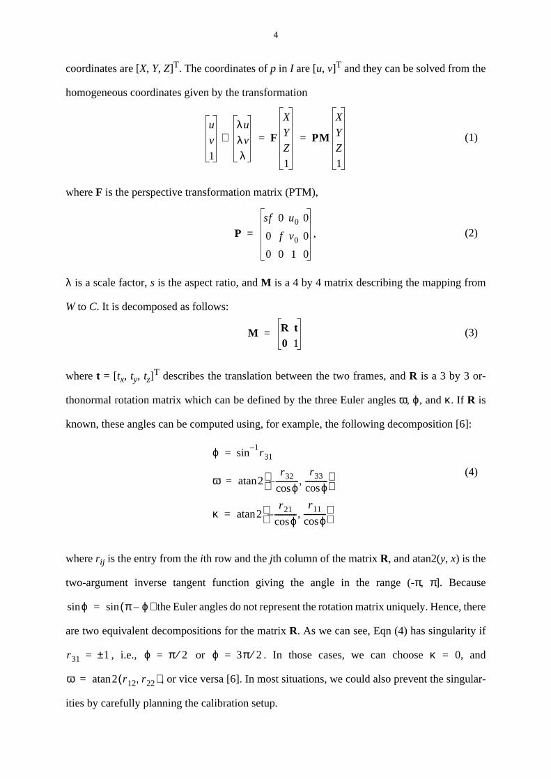
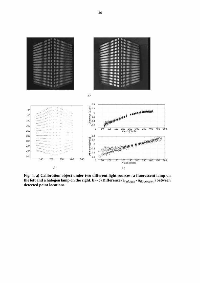
tions can also have a substantial effect on the calibration results. In Fig. 4 a) there are two im-

20

ages captured from exactly the same position and angle using the same camera settings, and

only the overall lighting has changed from fluorescent to halogen light. Fig. 4 b) shows the dif-

ference between the detected control point locations in the image plane. The difference is small-

est near the image center and increases radially when approaching the image borders. From Fig.

4 c) we notice that the difference is almost linear as a function of the horizontal and vertical co-

ordinates. The reason for this is chromatic aberration. According to Smith and Thomson [17]

chromatic aberration is a measurement of the spread of an image point over a range of colors.

It may be represented either as a longitudinal movement of an image plane, or as a change in

magnification, but basically it is a result of the dependence of the power of a refracting surface

on wavelength.

Camera electronics:Another type of systematic error is distinguished from Fig. 4c which is

the horizontal shift in the observed point locations. This shift is caused by a small change in the

overall intensity of lighting. The problem originates from the phase locked loop (PLL) opera-

tion, which is affected by the changes in the intensity level of the incoming light. According to

Beyer [18] detection of sync pulses is level sensitive and influenced by any changes on the sig-

nal level. This deviation is called line jitter, and it can be systematic as in Fig. 4c, or random

which is detected as increased observation noise in the horizontal image coordinates of the con-

trol points.

Calibration target: In the calibration procedure presented, it is assumed that the coordinates of

the 3-D control points are known with such precision that their errors are not observable from

the images. If this assumption is not met, the estimates of the camera parameters become inac-

curate. The relative accuracy in the object space should be better that the accuracy aspired to in

the image space. For example, if the goal is to achieve an accuracy of 1/50 of the pixel or around

1/50,000 of the image size, and if the dimensions of the calibration target are 100 mm by 100

mm in lateral directions, the 3-D coordinates of the circular control points should be known to

a resolution better than 2µm. Especially systematic errors that exceed the limit can cause sig-

nificant bias to the parameter estimates.

21

The effects of the error sources listed above are mixed in the observations and it is often

very difficult to recognize individual sources. However, the mixed effect of those sources that

are not compensated for by the camera model can be observed from the fitting residual as in-

creased random noise and as a systematic fluctuation. In [7], the systematic component of the

remaining error is calledanomalous distortion. In precise camera calibration, this component

should be so small that its influence on the parameter estimates becomes insignificant.

7 Conclusions

Geometric camera calibration is needed to describe the mapping between 3-D world coordi-

nates and 2-D image coordinates. An optimal calibration technique should produce unbiased

and minimum variance estimates of the camera parameters. In practice, this is quite difficult to

achieve due to different error sources affecting the imaging process. The calibration procedure

suggested in this paper utilizes circular control points and performs mapping from world coor-

dinates into image coordinates and backward from image coordinates to lines of sight or 3-D

plane coordinates. The camera model used allows least squares optimization with the distorted

image coordinates. The amount of computation is slightly increased with respect to the tradi-

tional camera model, but the number of the iterations needed in optimization remains the same

if weighting is not used. In the weighted least squares, the number of the iterations is doubled.

Experiments showed that an accuracy of 1/50 of the pixel size is achievable with this technique

if error sources, such as line jitter and chromatic aberration, are eliminated.

The camera calibration toolbox for Matlab used in the experiments is available in the

Internet athttp://www.ee.oulu.fi/~jth/calibr/.

Acknowledgements

The financial support of The Academy of Finland and The Graduate School in Electronics,

Telecommunications, and Automation (GETA) is gratefully acknowledged. The author is also

very grateful to the anonymous reviewers for valuable comments and suggestions.

22

8 References

[1] D. C. Brown, “Evolution, Application and Potential of the Bundle Method of

Photogrammetric Triangulation,”Proc. ISP Symposium, Stuttgart, Sept. 1974, pp. 69.

[2] R. Y. Tsai, “A versatile camera calibration technique for high-accuracy 3D machine

vision metrology using off-the-shelf TV cameras and lenses,”IEEE J. Robotics and

Automation, Vol. 3, No. 4, Aug. 1987, pp. 323-344.

[3] Y. I. Abdel-Aziz and H. M. Karara, “Direct linear transformation into object space

coordinates in close-range photogrammetry,”Proc. Symp. Close-Range

Photogrammetry, Urbana, Illinois, Jan. 1971, pp. 1-18.

[4] S. Ganapathy, “Decomposition of transformation matrices for robot vision,”Pattern

Recognition Letters, Vol. 2, 1984, pp. 401-412.

[5] O. D. Faugeras and G. Toscani, “Camera calibration for 3D computer vision,”Proc. Int’l

Workshop on Industrial Applications of Machine Vision and Machine Intelligence,

Tokyo, Japan, Feb. 1987, pp. 240-247.

[6] T. Melen, Geometrical modelling and calibration of video cameras for underwater

navigation, doctoral dissertation, Norwegian Univ. of Science and Technology,

Trondheim, Norway, 1994.

[7] C.C. Slama (ed.),Manual of Photogrammetry. 4th ed., American Society of

Photogrammetry, Falls Church, Virginia, 1980.

[8] H. Haggrén, “Photogrammetric machine vision,”Optics and Lasers in Engineering, Vol.

10, No. 3-4, 1989, pp. 265-286.

[9] R. K. Lenz and R. Y. Tsai, “Techniques for calibration of the scale factor and image center

for high accuracy 3-D machine vision metrology,”IEEE Trans. Pattern Analysis and

Machine Intelligence, Vol. 10, No. 5, 1988, pp. 713-720.

[10] J. Weng, P. Cohen and M. Herniou, “Camera calibration with distortion models and

accuracy evaluation,”IEEE Trans. Pattern Analysis and Machine Intelligence, Vol. 14,

No. 10, 1992, pp. 965-980.

23

[11] K. Kanatani,Geometric computation for Machine Vision, Oxford: Clarendon Press, 1993.

[12] W. H. Press, S. A. Teukolsky, W. T. Vetterling and B. P. Flannery,Numerical Recipes in

C - The Art of Scientific Computing. 2nd ed., Cambridge University Press, 1992.

[13] G. Strang,Linear algebra and its applications. 3rd ed., San Diego, CA: Harcourt Brace

Jovanovich, 1988.

[14] J. Heikkilä, “Moment and curvature preserving technique for accurate ellipse boundary

detection,”Proc. 14th Int’l Conf. on Pattern Recognition, Brisbane, Australia, Aug. 1998,

pp. 734-737.

[15] K. Kanatani, “Statistical bias of conic fitting and renormalization,”IEEE Trans. Pattern

Analysis and Machine Intelligence, Vol. 16, No. 3, 1994, pp. 320-326.

[16] R. G. Willson and S. A. Shafer, “What is the center of the image?”Proc. IEEE Conf.

Computer Vision and Pattern Recognition, New York, 1993, pp. 670-671.

[17] F. G. Smith and J. H. Thomson,Optics. 2nd ed., Wiley, Chichester, 1988.

[18] H. A. Beyer, “Linejitter and geometric calibration of CCD cameras,”ISPRS J.

Photogrammetry and Remote Sensing, Vol. 45, 1990, pp. 17-32.

24

uv

XY

Z

x

zy

f

projection centerO

ωκ

ϕimage planeΠ

object pointP

image pointp

Fig. 1. Pinhole camera model

camera frameC

world frameW

image frameI

Fig. 2. Calibration images: a) real, b) synthetic.

25

Fig. 3. The error of three different inverse distortion models a) as a function ofk1, b) asa function of k2, and c) the maximum distortion in the image coordinates fork1 and k2.

a)

b)

c)

26

a)

b) c)

Fig. 4. a) Calibration object under two different light sources: a fluorescent lamp onthe left and a halogen lamp on the right. b) - c) Difference (ahalogen - afluorescent) betweendetected point locations.

0 50 100 150 200 250 300 350 400 450 500

0 50 100 150 200 250 300 350 400 450 500

0.4

0.2

0

-0.2

-0.4

-0.6

0.4

0.2

0

-0.2

-0.4

-0.6

u-axis [pixels]

v-axis [pixels]

Diff

eren

ce [p

ixel

s]D

iffer

ence

[pix

els]

50

100

150

200

250

300

350

400

450

500100 200 300 400 500

27

Table 1. Estimated bias with confidence limits.

parameterunit

true value

estimated biasconf. min. (99%)conf. max. (99%)

method A method B method C

su 1.00377723 -0.00030584-0.00030696-0.00030473

0.000032370.000031260.00003348

0.000037400.000036480.00003832

f[mm]

8.345900 0.0051780.0051220.005233

-0.000064-0.000121-0.000007

-0.000168-0.000213-0.000124

u0[pixels]

367.3353 -0.0096-0.0170-0.0022

0.00900.00170.0163

0.02210.01620.0280

v0[pixels]

305.9960 0.48790.47750.4983

-0.0175-0.0280-0.0070

-0.0343-0.0429-0.0256

k1 (. 10-3)

[mm-2]

3.29545 -0.06682-0.06730-0.06634

-0.00953-0.01001-0.00904

-0.01034-0.01079-0.00988

k2 (. 10-5)

[mm-4]

-2.6287 0.48290.47960.4863

0.09020.08700.0934

0.10090.09770.1040

p1 (. 10-5)

[mm-1]

-0.13 -1.996-2.030-1.962

-1.386-1.419-1.352

-1.370-1.401-1.339

p2 (. 10-5)

[mm-1]

4.065 -1.228-1.249-1.206

-1.201-1.222-1.180

-1.237-1.257-1.217

28

Table 2. Estimated standard deviation with confidence limits.

parameterunit

theoretical std

estimated stdconf. min. (95%)conf. max. (95%)

method A method B method C

su 0.00000417 0.000008020.000007310.00000890

0.000007970.000007260.00000885

0.000006590.000006010.00000732

f[mm]

0.000210 0.0003980.0003620.000442

0.0004100.0003740.000456

0.0003210.0002920.000356

u0[pixels]

0.0261 0.05300.04830.0588

0.05220.04760.0580

0.04240.03860.0471

v0[pixels]

0.0366 0.07480.06820.0831

0.07530.06870.0836

0.06220.05670.0691

k1 (. 10-3)

[mm-2]

0.00196 0.003470.003160.00385

0.003470.003170.00386

0.003280.002990.00365

k2 (. 10-5)

[mm-4]

0.0138 0.02390.02180.0265

0.02330.02120.0259

0.02270.02070.0253

p1 (. 10-5)

[mm-1]

0.132 0.2430.2210.270

0.2420.2200.268

0.2220.2030.247

p2 (. 10-5)

[mm-1]

0.087 0.1540.1410.171

0.1480.1350.165

0.1440.1310.160

29

Janne Heikkilä received the MSc degree in electrical engineeringfrom the University of Oulu, Finland, in 1993, and the PhD degreein computer science in 1998. Since September 1998, he has been apost-doctoral fellow in Machine Vision and Media ProcessingUnit at the University of Oulu. His research interests include cam-era based precise 3-D measurements, geometric camera calibra-tion, human tracking from image sequences, and motionestimation.