Geometric Algebra equivalants for Pauli Matrices.

Peeter Joot — peeter.joot@gmail.comDec 06, 2008 RCS f ile : pauliMatrix.tex, v Last Revision : 1.27 Date : 2009/07/1214 : 07 : 04

Contents

1 Motivation. 2

2 Pauli Matrices 22.1 Pauli Vector. . . . . . . . . . . . . . . . . . . . . . . . . . . . . . . . . . . . . . . . . . . 22.2 Matrix squares . . . . . . . . . . . . . . . . . . . . . . . . . . . . . . . . . . . . . . . . . 32.3 Length . . . . . . . . . . . . . . . . . . . . . . . . . . . . . . . . . . . . . . . . . . . . . 3

2.3.1 Aside: Summarizing the multiplication table. . . . . . . . . . . . . . . . . . . . 52.4 Scalar product. . . . . . . . . . . . . . . . . . . . . . . . . . . . . . . . . . . . . . . . . . 52.5 Symmetric and antisymmetric split. . . . . . . . . . . . . . . . . . . . . . . . . . . . . 62.6 Vector inverse. . . . . . . . . . . . . . . . . . . . . . . . . . . . . . . . . . . . . . . . . . 72.7 Coordinate extraction. . . . . . . . . . . . . . . . . . . . . . . . . . . . . . . . . . . . . 82.8 Projection and rejection. . . . . . . . . . . . . . . . . . . . . . . . . . . . . . . . . . . . 82.9 Space of the vector product. . . . . . . . . . . . . . . . . . . . . . . . . . . . . . . . . . 92.10 Completely antisymmetrized product of three vectors. . . . . . . . . . . . . . . . . . 102.11 Duality. . . . . . . . . . . . . . . . . . . . . . . . . . . . . . . . . . . . . . . . . . . . . . 112.12 Complete algebraic space. . . . . . . . . . . . . . . . . . . . . . . . . . . . . . . . . . . 122.13 Reverse operation. . . . . . . . . . . . . . . . . . . . . . . . . . . . . . . . . . . . . . . 142.14 Rotations. . . . . . . . . . . . . . . . . . . . . . . . . . . . . . . . . . . . . . . . . . . . 142.15 Grade selection. . . . . . . . . . . . . . . . . . . . . . . . . . . . . . . . . . . . . . . . . 152.16 Generalized dot products. . . . . . . . . . . . . . . . . . . . . . . . . . . . . . . . . . . 162.17 Generalized dot and wedge product. . . . . . . . . . . . . . . . . . . . . . . . . . . . . 17

2.17.1 Grade zero. . . . . . . . . . . . . . . . . . . . . . . . . . . . . . . . . . . . . . . 172.17.2 Grade one. . . . . . . . . . . . . . . . . . . . . . . . . . . . . . . . . . . . . . . . 182.17.3 Grade two. . . . . . . . . . . . . . . . . . . . . . . . . . . . . . . . . . . . . . . . 192.17.4 Grade three. . . . . . . . . . . . . . . . . . . . . . . . . . . . . . . . . . . . . . . 19

2.18 Plane projection and rejection. . . . . . . . . . . . . . . . . . . . . . . . . . . . . . . . . 20

3 Examples. 213.1 Radial decomposition. . . . . . . . . . . . . . . . . . . . . . . . . . . . . . . . . . . . . 21

3.1.1 Velocity and momentum. . . . . . . . . . . . . . . . . . . . . . . . . . . . . . . 213.1.2 Acceleration and force. . . . . . . . . . . . . . . . . . . . . . . . . . . . . . . . . 22

4 Conclusion. 23

1

1. Motivation.

Having learned Geometric (Clifford) Algebra from ([1]), ([2]), ([3]), and other sources beforestudying any quantum mechanics, trying to work with (and talk to people familiar with) the Pauliand Dirac matrix notation as used in traditional quantum mechanics becomes difficult.

The aim of these notes is to work through equivalents to many Clifford algebra expressionsentirely in commutator and anticommutator notations. This will show the mapping between the(generalized) dot product and the wedge product, and also show how the different grade elementsof the Clifford algebra Cl(3, 0) manifest in their matrix forms.

2. Pauli Matrices

The matrices in question are:

σ1 =[

0 11 0

](1)

σ2 =[

0 −ii 0

](2)

σ3 =[

1 00 −1

](3)

These all have positive square as do the traditional Euclidean unit vectors ei, and so can beused algebraically as a vector basis for R3. So any vector that we can write in coordinates

x = xiei,

we can equivalently write (an isomorphism) in terms of the Pauli matrix’s

x = xiσi. (4)

2.1. Pauli Vector.

([4]) introduces the Pauli vector as a mechanism for mapping between a vector basis and thismatrix basis

σ = ∑ σiei

This is a curious looking construct with products of 2x2 matrices and R3 vectors. Obviouslythese are not the usual 3x1 column vector representations. This Pauli vector is thus really a nota-tional construct. If one takes the dot product of a vector expressed using the standard orthonormalEuclidean basis {ei} basis, and then takes the dot product with the Pauli matrix in a mechanicalfashion

2

x · σ = (xiei) ·∑ σjej

= ∑i,j

xiσjei · ej

= xiσi

one arrives at the matrix representation of the vector in the Pauli basis {σi}. Does this constructhave any value? That I don’t know, but for the rest of these notes the coordinate representation asin equation (4) will be used directly.

2.2. Matrix squares

It was stated that the Pauli matrices have unit square. Direct calculation of this is straightfor-ward, and confirms the assertion

σ12 =

[0 11 0

] [0 11 0

]=[

1 00 1

]= I

σ22 =

[0 −ii 0

] [0 −ii 0

]= i2

[0 −11 0

] [0 −11 0

]=[

1 00 1

]= I

σ32 =

[1 00 −1

] [1 00 −1

]=[

1 00 1

]= I

Note that unlike the vector (Clifford) square the identity matrix and not a scalar.

2.3. Length

If we are to operate with Pauli matrices how do we express our most basic vector operation,the length?

Examining a vector lying along one direction, say, a = αx we expect

a2 = a · a = α2x · x = α2.

Lets contrast this to the Pauli square for the same vector y = ασ1

y2 = α2σ12 = α2 I

The wiki article mentions trace, but no application for it. Since Tr (I) = 2, an observableapplication is that the trace operator provides a mechanism to convert a diagonal matrix to ascalar. In particular for this scaled unit vector y we have

α2 =12

Tr(y2)

3

It is plausible to guess that the squared length will be related to the matrix square in the generalcase as well

|x|2 =12

Tr(x2)

Let’s see if this works by performing the coordinate expansion

x2 = (xiσi)(xjσj)

= xixjσiσj

A split into equal and different indexes thus leaves

x2 = ∑i<j

xixj(σiσj + σjσi) + ∑i(xi)2σi

2 (5)

As an algebra that is isomorphic to the Clifford Algebra C{3,0} it is expected that the σiσj matri-ces anticommute for i 6= j. Multiplying these out verifies this

σ1σ2 = i[

0 11 0

] [0 −11 0

]= i[

1 00 −1

]= iσ3

σ2σ1 = i[

0 −11 0

] [0 11 0

]= i[−1 00 1

]= −iσ3

σ3σ1 =[

1 00 −1

] [0 11 0

]=[

0 1−1 0

]= iσ2

σ1σ3 =[

0 11 0

] [1 00 −1

]=[

0 −11 0

]= −iσ2

σ2σ3 = i[

0 −11 0

] [1 00 −1

]= i[

0 11 0

]= iσ1

σ3σ2 = i[

1 00 −1

] [0 −11 0

]= i[

0 −1−1 0

]= −iσ3

.

Thus in (5) the sum over the {i < j} = {12, 23, 13} indexes is zero.Having computed this, our vector square leaves us with the vector length multiplied by the

identity matrix

x2 = ∑i(xi)2 I.

Invoking the trace operator will therefore extract just the scalar length desired

|x|2 =12

Tr(x2) = ∑

i(xi)2. (6)

4

2.3.1 Aside: Summarizing the multiplication table.

It is worth pointing out that the multiplication table above used to confirm the antisymmetricbehavior of the Pauli basis can be summarized as

σaσb = 2iεabcσc (7)

2.4. Scalar product.

Having found the expression for the length of a vector in the Pauli basis, the next logicaldesirable identity is the dot product. One can guess that this will be the trace of a scaled symmetricproduct, but can motivate this without guessing in the usual fashion, by calculating the length ofan orthonormal sum.

Consider first the length of a general vector sum. To calculate this we first wish to calculate thematrix square of this sum.

(x + y)2 = x2 + y2 + xy + yx

If these vectors are perpendicular this equals x2 + y2. Thus orthonormality implies that

xy + yx = 0

or,

yx = −xy (8)

We have already observed this by direct calculation for the Pauli matrices themselves. Now,this is not any different than the usual description of perpendicularity in a Clifford Algebra, andit is notable that there are not any references to matrices in this argument. One only requires thata well defined vector product exists, where the squared vector has a length interpretation.

One matrix dependent observation that can be made is that since the left hand side and thex2, and y2 terms are all diagonal, this symmetric sum must also be diagonal. Additionally, for thelength of this vector sum we then have

|x + y|2 = |x|2 + |y|2 +12

Tr (xy + yx)

For correspondence with the Euclidean dot product of two vectors we must then have

x • y =14

Tr (xy + yx) . (9)

5

Here x • y has been used to denote this scalar product (ie: a plain old number), since x · y willbe used later for a matrix dot product (this times the identity matrix) which is more natural inmany ways for this Pauli algebra.

Observe the symmetric product that is found embedded in this scalar selection operation. Inphysics this is known as the anticommutator, where the commutator is the antisymmetric sum. Inthe physics notation the anticommutator (symmetric sum) is

{x, y} = xy + yx (10)

So this scalar selection can be written

x • y =14

Tr {x, y} (11)

Similarly, the commutator, an antisymmetric product, is denoted:

[x, y] = xy − yx, (12)

A close relationship between this commutator and the wedge product of Clifford Algebra isexpected.

2.5. Symmetric and antisymmetric split.

As with the Clifford product, the symmetric and antisymmetric split of a vector product is auseful concept. This can be used to write the product of two Pauli basis vectors in terms of theanticommutator and commutator products

xy =12{x, y}+

12

[x, y] (13)

yx =12{x, y} − 1

2[x, y] (14)

These follows from the definition of the anticommutator (10) and commutator (12) productsabove, and are the equivalents of the Clifford symmetric and antisymmetric split into dot andwedge products

xy = x · y + x ∧ y (15)yx = x · y − x ∧ y (16)

Where the dot and wedge products are respectively

x · y =12(xy + yx)

x ∧ y =12(xy − yx)

6

Note the factor of two differences in the two algebraic notations. In particular very handyClifford vector product reversal formula

yx = −xy + 2x · y

has no factor of two in its Pauli anticommutator equivalent

yx = −xy + {x, y} (17)

2.6. Vector inverse.

It has been observed that the square of a vector is diagonal in this matrix representation, andcan therefore be inverted for any non-zero vector

x2 = |x|2 I

(x2)−1 = |x|−2 I=⇒

x2(x2)−1 = I

So it is therefore quite justifiable to define

x−2 =1x2 ≡ |x|−2 I

This allows for the construction of a dual sided vector inverse operation.

x−1 ≡ 1

|x|2x

=1x2 x

= x1x2

This inverse is a scaled version of the vector itself.The diagonality of the squared matrix or the inverse of that allows for commutation with x.

This diagonality plays the same role as the scalar in a regular Clifford square. In either case thesquare can commute with the vector, and that commutation allows the inverse to have both leftand right sided action.

Note that like the Clifford vector inverse when the vector is multiplied with this inverse, theproduct resides outside of the proper R3 Pauli basis since the identity matrix is required.

7

2.7. Coordinate extraction.

Given a vector in the Pauli basis, we can extract the coordinates using the scalar product

x = ∑i

14

Tr {x, σi}σi

But do not need to convert to strict scalar form if we are multiplying by a Pauli matrix. So inanticommutator notation this takes the form

x = xiσi = ∑i

12{x, σi}σi (18)

xi =12{x, σi} (19)

2.8. Projection and rejection.

The usual Clifford algebra trick for projective and rejective split maps naturally to matrix form.Write

x = xaa−1

= (xa)a−1

=(

12{x, a}+

12

[x, a])

a−1

=(

12

(xa + ax) +12

(xa − ax))

a−1

=12

(x + axa−1

)+

12

(x − axa−1

)

Since {x, a} is diagonal, this first term is proportional to a−1, and thus lines in the direction ofa itself. The second term is perpendicular to a.

These are in fact the projection of x in the direction of a and rejection of x from the direction ofa respectively.

x = x‖ + x⊥

x‖ = Proja(x) =12{x, a}a−1 =

12

(x + axa−1

)x⊥ = Reja(x) =

12

[x, a] a−1 =12

(x − axa−1

)

To complete the verification of this note that the perpendicularity of the x⊥ term can be verifiedby taking dot products

8

12{a, x⊥} =

14

(a(

x − axa−1)

+(

x − axa−1)

a)

=14

(ax − aaxa−1 + xa − axa−1a

)=

14

(ax − xa + xa − ax)

= 0

2.9. Space of the vector product.

Expansion of the anticommutator and commutator in coordinate form shows that these entitieslie in a different space than the vectors itself.

For real coordinate vectors in the Pauli basis, all the commutator values are imaginary multi-ples and thus not representable

[x, y] = xaσaybσb − yaσaxbσb

= (xayb − yaxb)σaσb

= 2i(xayb − yaxb)εabcσc

Similarly, the anticommutator is diagonal, which also falls outside the Pauli vector basis:

{x, y} = xaσaybσb + yaσaxbσb

= (xayb + yaxb)σaσb

= (xayb + yaxb)(Iδab + iεabcσc)

= ∑a

(xaya + yaxa)I + ∑a<b

(xayb + yaxb)i(εabc + εbac︸ ︷︷ ︸=0

)σc

= ∑a

(xaya + yaxa)I

= 2 ∑a

xaya I,

These correspond to the Clifford dot product being scalar (grade zero), and the wedge defininga grade two space, where grade expresses the minimal degree that a product can be reduced to.By example a Clifford product of normal unit vectors such as

e1e3e4e1e3e4e3 ∝ e3

e2e3e4e1e3e4e3e5 ∝ e1e2e3e5

are grade one and four respectively. The proportionality constant will be dependent on metricof the underlying vector space and the number of permutations required to group terms in pairsof matching indexes.

9

2.10. Completely antisymmetrized product of three vectors.

In a Clifford algebra no imaginary number is required to express the antisymmetric (commu-tator) product. However, the bivector space can be enumerated using a dual basis defined bymultiplication of the vector basis elements with the unit volume trivector. That is also the casehere and gives a geometrical meaning to the imaginaries of the Pauli formulation.

How do we even write the unit volume element in Pauli notation? This would be

σ1 ∧ σ2 ∧ σ3 = (σ1 ∧ σ2) ∧ σ3

=12

[σ1, σ2] ∧ σ3

=14

([σ1, σ2] σ3 + σ3 [σ1, σ2])

So we have

σ1 ∧ σ2 ∧ σ3 =18{[σ1, σ2] , σ3} (20)

Similar expansion of σ1 ∧ σ2 ∧ σ3 = σ1 ∧ (σ2 ∧ σ3), or σ1 ∧ σ2 ∧ σ3 = (σ3 ∧ σ1) ∧ σ2 shows thatwe must also have

{[σ1, σ2] , σ3} = {σ1, [σ2, σ3]} = {[σ3, σ1] , σ2} (21)

Until now the differences in notation between the anticommutator/commutator and the dot/wedgeproduct of the Pauli algebra and Clifford algebra respectively have only differed by factors of two,which isn’t much of a big deal. However, having to express the naturally associative wedge prod-uct operation in the non-associative looking notation of equation (20) is rather unpleasant seem-ing. Looking at an expression of the form gives no mnemonic hint of the underlying associativity,and actually seems obfuscating. I suppose that one could get used to it though.

We expect to get a three by three determinant out of the trivector product. Let’s verify this byexpanding this in Pauli notation for three general coordinate vectors

{[x, y] , z} ={[

xaσa, ybσb

], zcσc

}= 2iεabdxaybzc{σd, σc}= 4iεabdxaybzcδcd I

= 4iεabcxaybzc I

= 4i

∣∣∣∣∣∣xa xb xcya yb ycza zb zc

∣∣∣∣∣∣ I

In particular, our unit volume element is

σ1 ∧ σ2 ∧ σ3 =14{[σ1, σ2] , σ3} = iI (22)

10

So one sees that the complex number i in the Pauli algebra can logically be replaced by the unitpseudoscalar iI, and relations involving i, like the commutator expansion of a vector product, isrestored to the expected dual form of Clifford algebra

σa ∧ σb =12

[σa, σb]

= iεabcσc

= (σa ∧ σb ∧ σc)σc

Or

σa ∧ σb = (σa ∧ σb ∧ σc) · σc (23)

2.11. Duality.

We’ve seen that multiplication by i is a duality operation, which is expected since iI is thematrix equivalent of the unit pseudoscalar. Logically this means that for a vector x, the product(iI)x represents a plane quantity (torque, angular velocity/momentum, ...). Similarly if B is aplane object, then (iI)B will have a vector interpretation.

In particular, for the antisymmetric (commutator) part of the vector product xy

12

[x, y] =12

xayb [σa, σb]

= xaybiεabcσc

a “vector” in the dual space spanned by {iσa} is seen to be more naturally interpreted as aplane quantity (bivector in Clifford algebra).

As in Clifford algebra, we can write the cross product in terms of the antisymmetric product

a × b =12i

[a, b] .

With the factor of 2 in the denominator here (like the exponential form of sine), it is interestingto contrast this to the cross product in its trigonometric form

a × b = |a||b| sin(θ)n

= |a||b| 12i

(eiθ − e−iθ)n

This shows we can make the curious identity

[a, b]

= (eiθ − e−iθ)n

If one did not already know about the dual sides half angle rotation formulation of Clifford al-gebra, this is a hint about how one could potentially work towards that. We have the commutator(or wedge product) as a rotation operator that leaves the normal component of a vector untouched(commutes with the normal vector).

11

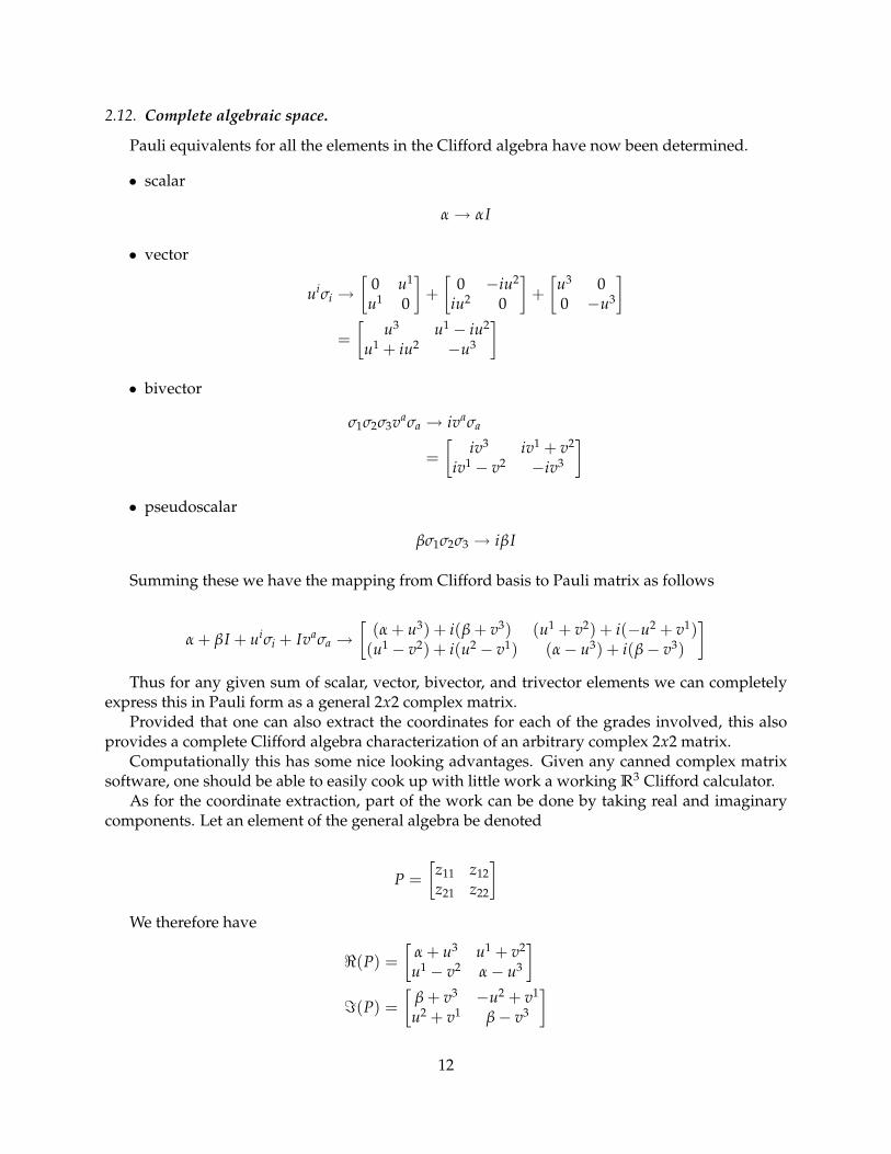
2.12. Complete algebraic space.

Pauli equivalents for all the elements in the Clifford algebra have now been determined.

• scalar

α → αI

• vector

uiσi →[

0 u1

u1 0

]+[

0 −iu2

iu2 0

]+[

u3 00 −u3

]=[

u3 u1 − iu2

u1 + iu2 −u3

]• bivector

σ1σ2σ3vaσa → ivaσa

=[

iv3 iv1 + v2

iv1 − v2 −iv3

]• pseudoscalar

βσ1σ2σ3 → iβI

Summing these we have the mapping from Clifford basis to Pauli matrix as follows

α + βI + uiσi + Ivaσa →[

(α + u3) + i(β + v3) (u1 + v2) + i(−u2 + v1)(u1 − v2) + i(u2 − v1) (α − u3) + i(β − v3)

]Thus for any given sum of scalar, vector, bivector, and trivector elements we can completely

express this in Pauli form as a general 2x2 complex matrix.Provided that one can also extract the coordinates for each of the grades involved, this also

provides a complete Clifford algebra characterization of an arbitrary complex 2x2 matrix.Computationally this has some nice looking advantages. Given any canned complex matrix

software, one should be able to easily cook up with little work a working R3 Clifford calculator.As for the coordinate extraction, part of the work can be done by taking real and imaginary

components. Let an element of the general algebra be denoted

P =[

z11 z12z21 z22

]We therefore have

<(P) =[

α + u3 u1 + v2

u1 − v2 α − u3

]=(P) =

[β + v3 −u2 + v1

u2 + v1 β − v3

]

12

By inspection, symmetric and antisymmetric sums of the real and imaginary parts recovers thecoordinates as follows

α =12<(z11 + z22)

u3 =12<(z11 − z22)

u1 =12<(z12 + z21)

v2 =12<(z12 − z21)

β =12=(z11 + z22)

v3 =12=(z11 − z22)

v1 =12=(z12 + z21)

u2 =12=(−z12 + z21)

In terms of grade selection operations the decomposition by grade

P = 〈P〉 + 〈P〉1 + 〈P〉2 + 〈P〉3,

is

〈P〉 =12<(z11 + z22) =

12<(Tr P)

〈P〉1 =12

(<(z12 + z21)σ1 +=(−z12 + z21)σ2 +<(z11 − z22)σ3)

〈P〉2 =12

(=(z12 + z21)σ2 ∧ σ3 +<(z12 − z21)σ3 ∧ σ1 +=(z11 − z22)σ1 ∧ σ2)

〈P〉3 =12=(z11 + z22)I =

12=(Tr P)σ1 ∧ σ2 ∧ σ3

Employing =(z) = <(−iz), and <(z) = =(iz) this can be made slightly more symmetri-cal, with Real operations selecting the vector coordinates and imaginary operations selecting thebivector coordinates.

〈P〉 =12<(z11 + z22) =

12<(Tr P)

〈P〉1 =12

(<(z12 + z21)σ1 +<(iz12 − iz21)σ2 +<(z11 − z22)σ3)

〈P〉2 =12

(=(z12 + z21)σ2 ∧ σ3 +=(iz12 − iz21)σ3 ∧ σ1 +=(z11 − z22)σ1 ∧ σ2)

〈P〉3 =12=(z11 + z22)I =

12=(Tr P)σ1 ∧ σ2 ∧ σ3

13

Finally, returning to the Pauli algebra, this also provides the following split of the Pauli multi-vector matrix into its geometrically significant components P = 〈P〉 + 〈P〉1 + 〈P〉2 + 〈P〉3,

〈P〉 =12<(z11 + z22)I

〈P〉1 =12

(<(z12 + z21)σ1 +<(iz12 − iz21)σ2 +<(z11 − z22)σ3)

〈P〉2 =12

(=(z12 + z21)iσ1 +=(iz12 − iz21)iσ2 +=(z11 − z22)iσk)

〈P〉3 =12=(z11 + z22)iI

2.13. Reverse operation.

The reversal operation switches the order of the product of perpendicular vectors. This willchange the sign of grade two and three terms in the Pauli algebra. Since σ2 is imaginary, conju-gation does not have the desired effect, but Hermitian conjugation (conjugate transpose) does thetrick.

Since the reverse operation can be written as Hermitian conjugation, one can also define theanticommutator and commutator in terms of reversion in a way that seems particularly naturalfor complex matrices. That is

{a, b} = ab + (ab)∗ (24)[a, b] = ab − (ab)∗ (25)

(26)

2.14. Rotations.

Rotations take the normal Clifford, dual sided quaterionic form. A rotation about a unit normaln will be

R(x) = e−inθ/2xeinθ/2

The Rotor R = e−inθ/2 commutes with any component of the vector x that is parallel to thenormal (perpendicular to the plane), whereas it anticommutes with the components in the plane.Writing the vector components perpendicular and parallel to the plane respectively as x = x⊥ +x‖, the essence of the rotation action is this selective commutation or anti-commutation behavior

Rx‖R∗ = x‖R∗

Rx⊥R∗ = x⊥RR∗ = x⊥

Here the exponential has the obvious meaning in terms of exponential series, so for this bivec-tor case we have

exp(inθ/2) = cos(θ/2)I + in sin(θ/2)

14

The unit bivector B = in can also be defined explicitly in terms of two vectors a, and b in theplane

B =1

|[a, b]| [a, b]

Where the bivector length is defined in terms of the conjugate square (bivector times bivectorreverse)

|[a, b]|2 = [a, b] [a, b]∗

Examples to complete this subsection would make sense. As one of the most powerful anduseful operations in the algebra, it is a shame in terms of completeness to skimp on this. How-ever, except for some minor differences like substitution of the Hermitian conjugate operation forreversal, the use of the identity matrix I in place of the scalar in the exponential expansion, thetreatment is exactly the same as in the Clifford algebra.

2.15. Grade selection.

Coordinate equations for grade selection were worked out above, but the observation thatreversion and Hermitian conjugation are isomorphic operations can partially clean this up. Inparticular a Hermitian conjugate symmetrization and anti-symmetrization of the general matrixprovides a nice split into quaternion and dual quaternion parts (say P = Q + R respectively). Thatis

Q = 〈P〉 + 〈P〉1 =12(P + P∗)

R = 〈P〉2 + 〈P〉3 =12(P − P∗)

Now, having done that, how to determine 〈Q〉, 〈Q〉1, 〈R〉2, and 〈R〉3 becomes the next question.Once that is done, the individual coordinates can be picked off easily enough. For the vector parts,a Fourier decomposition as in equation (18) will retrieve the desired coordinates.

The dual vector coordinates can be picked off easily enough taking dot products with the dualbasis vectors

B = Bkiσk = ∑k

12

{B,

1iσk

}iσk (27)

Bk =12

{B,

1iσk

}(28)

For the quaternion part Q the aim is to figure out how to isolate or subtract out the scalar part.This is the only tricky bit because the diagonal bits are all mixed up with the σ3 term which is alsoreal, and diagonal. Consideration of the sum

aI + bσ3 =[

a + b 00 a − b

],

15

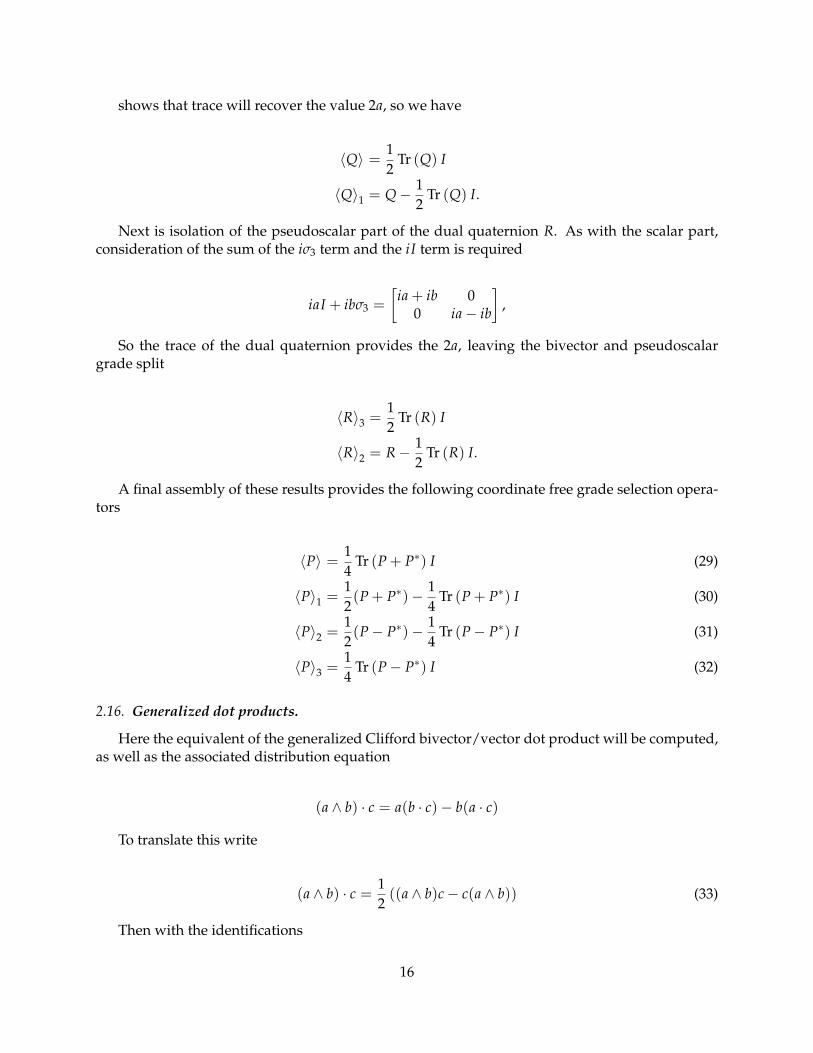
shows that trace will recover the value 2a, so we have

〈Q〉 =12

Tr (Q) I

〈Q〉1 = Q − 12

Tr (Q) I.

Next is isolation of the pseudoscalar part of the dual quaternion R. As with the scalar part,consideration of the sum of the iσ3 term and the iI term is required

iaI + ibσ3 =[

ia + ib 00 ia − ib

],

So the trace of the dual quaternion provides the 2a, leaving the bivector and pseudoscalargrade split

〈R〉3 =12

Tr (R) I

〈R〉2 = R − 12

Tr (R) I.

A final assembly of these results provides the following coordinate free grade selection opera-tors

〈P〉 =14

Tr (P + P∗) I (29)

〈P〉1 =12(P + P∗)− 1

4Tr (P + P∗) I (30)

〈P〉2 =12(P − P∗)− 1

4Tr (P − P∗) I (31)

〈P〉3 =14

Tr (P − P∗) I (32)

2.16. Generalized dot products.

Here the equivalent of the generalized Clifford bivector/vector dot product will be computed,as well as the associated distribution equation

(a ∧ b) · c = a(b · c)− b(a · c)

To translate this write

(a ∧ b) · c =12

((a ∧ b)c − c(a ∧ b)) (33)

Then with the identifications

16

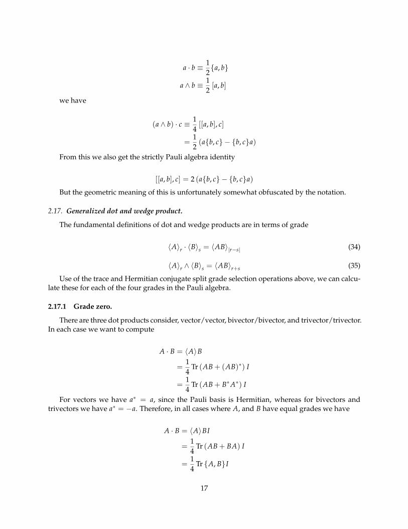
a · b ≡ 12{a, b}

a ∧ b ≡ 12

[a, b]

we have

(a ∧ b) · c ≡ 14

[[a, b], c]

=12

(a{b, c} − {b, c}a)

From this we also get the strictly Pauli algebra identity

[[a, b], c] = 2 (a{b, c} − {b, c}a)

But the geometric meaning of this is unfortunately somewhat obfuscated by the notation.

2.17. Generalized dot and wedge product.

The fundamental definitions of dot and wedge products are in terms of grade

〈A〉r · 〈B〉s = 〈AB〉|r−s| (34)

〈A〉r ∧ 〈B〉s = 〈AB〉r+s (35)

Use of the trace and Hermitian conjugate split grade selection operations above, we can calcu-late these for each of the four grades in the Pauli algebra.

2.17.1 Grade zero.

There are three dot products consider, vector/vector, bivector/bivector, and trivector/trivector.In each case we want to compute

A · B = 〈A〉B

=14

Tr (AB + (AB)∗) I

=14

Tr (AB + B∗A∗) I

For vectors we have a∗ = a, since the Pauli basis is Hermitian, whereas for bivectors andtrivectors we have a∗ = −a. Therefore, in all cases where A, and B have equal grades we have

A · B = 〈A〉BI

=14

Tr (AB + BA) I

=14

Tr {A, B}I

17

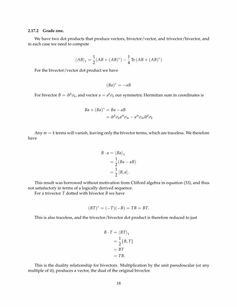
2.17.2 Grade one.

We have two dot products that produce vectors, bivector/vector, and trivector/bivector, andin each case we need to compute

〈AB〉1 =12(AB + (AB)∗)− 1

4Tr (AB + (AB)∗)

For the bivector/vector dot product we have

(Ba)∗ = −aB

For bivector B = ibkσk, and vector a = akσk our symmetric Hermitian sum in coordinates is

Ba + (Ba)∗ = Ba − aB

= ibkσkamσm − amσmibkσk

Any m = k terms will vanish, leaving only the bivector terms, which are traceless. We thereforehave

B · a = 〈Ba〉1

=12(Ba − aB)

=12

[B, a] .

This result was borrowed without motivation from Clifford algebra in equation (33), and thusnot satisfactory in terms of a logically derived sequence.

For a trivector T dotted with bivector B we have

(BT)∗ = (−T)(−B) = TB = BT.

This is also traceless, and the trivector/bivector dot product is therefore reduced to just

B · T = 〈BT〉1

=12{B, T}

= BT= TB.

This is the duality relationship for bivectors. Multiplication by the unit pseudoscalar (or anymultiple of it), produces a vector, the dual of the original bivector.

18

2.17.3 Grade two.

We have two products that produce a grade two term, the vector wedge product, and thevector/trivector dot product. For either case we must compute

〈AB〉2 =12(AB − (AB)∗)− 1

4Tr (AB − (AB)∗) (36)

For a vector a, and trivector T we need the antisymmetric Hermitian sum

aT − (aT)∗ = aT + Ta = 2aT = 2Ta

This is a pure bivector, and thus traceless, leaving just

a · T = 〈aT〉2 (37)= aT (38)= Ta (39)

Again we have the duality relation, pseudoscalar multiplication with a vector produces abivector, and is equivalent to the dot product of the two.

Now for the wedge product case, with vector a = amσm, and b = bkσk we must compute

ab − (ab)∗ = ab − ba

= amσmbkσk − bkσkamσm

All the m = n terms vanish, leaving a pure bivector which is traceless, so only the first term of(36) is relevant, and is in this case a commutator

a ∧ b = 〈ab〉2 (40)

=12

[a, b] (41)

2.17.4 Grade three.

There are two ways we can produce a grade three term in the algebra. One is a wedge ofa vector with a bivector, and the other is the wedge product of three vectors. The triple wedgeproduct is the grade three term of the product of the three

a ∧ b ∧ c = 〈abc〉3

=14

Tr (abc − (abc)∗)

=14

Tr (abc − cba)

19

With a split of the bc and cb terms into symmetric and antisymmetric terms we have

abc − cba =12(a{b, c} − {c, b}a) +

12(a [b, c]− [c, b] a)

The symmetric term is diagonal so it commutes (equivalent to scalar commutation with a vec-tor in Clifford algebra), and this therefore vanishes. Writing B = b ∧ c = 1

2 [b, c], and noting that[b, c] = − [c, b] we therefore have

a ∧ B = 〈aB〉3

=14

Tr (aB + Ba)

=14

Tr {a, B}

In terms of the original three vectors this is

a ∧ b ∧ c = 〈aB〉3

=18

Tr {a, [b, c]}.

Since this could have been expanded by grouping ab instead of bc we also have

a ∧ b ∧ c =18

Tr {[a, b] , c}.

2.18. Plane projection and rejection.

Projection of a vector onto a plane follows like the vector projection case. In the Pauli notationthis is

x = xB1B

=12{x, B} 1

B+

12

[x, B]1B

Here the plane is a bivector, so if vectors a, and b are in the plane, the orientation and attitudecan be represented by the commutator

So we have

x =12{x, [a, b]} 1

[a, b]+

12

[x, [a, b]]1

[a, b]

Of these the second term is our projection onto the plane, while the first is the normal compo-nent of the vector.

20

3. Examples.

3.1. Radial decomposition.

3.1.1 Velocity and momentum.

A decomposition of velocity into radial and perpendicular components should be straightfor-ward in the Pauli algebra as it is in the Clifford algebra.

With a radially expressed position vector

x = |x|x,

velocity can be written by taking derivatives

v = x′ = |x|′ x + |x|x′

or as above in the projection calculation with

v = v1x

x

=12

{v,

1x

}x +

12

[v,

1x

]x

=12{v, x}x +

12

[v, x] x

By comparison we have

|x|′ =12{v, x}

x′ =1

2|x| [v, x] x

In assembled form we have

v =12{v, x}x + xω

Here the commutator has been identified with the angular velocity bivector ω

ω =1

2x2 [x, v] .

Similarly, the linear and angular momentum split of a momentum vector is

p‖ =12{p, x}x

p⊥ =12

[p, x] x

21

and in vector form

p =12{p, x}x + mxω

Writing J = mx2 for the moment of inertia we have for our commutator

L =12

[x, p] = mx2ω = Jω

With the identification of the commutator with the angular momentum bivector L we have thetotal momentum as

p =12{p, x}x +

1x

L

3.1.2 Acceleration and force.

Having computed velocity, and its radial split, the next logical thing to try is acceleration.The acceleration will be

a = v′ = |x|′′ x + 2|x|′ x′ + |x|x′′

We need to compute x′′ to continue, which is

x′′ =

(1

2|x|3[v, x] x

)′

=−3

2|x|4|x|′ [v, x] x +

1

2|x|3[a, x] x +

1

2|x|3[v, x] v

=−3

4|x|5{v, x} [v, x] x +

1

2|x|3[a, x] x +

1

2|x|3[v, x] v

Putting things back together is a bit messy, but starting so gives

a = |x|′′ x + 21

4|x|4{v, x} [v, x] x +

−3

4|x|4{v, x} [v, x] x +

1

2|x|2[a, x] x +

1

2|x|2[v, x] v

= |x|′′ x − 1

4|x|4{v, x} [v, x] x +

1

2|x|2[a, x] x +

1

2|x|2[v, x] v

= |x|′′ x +1

4|x|4[v, x]

(−{v, x}x + 2x2v

)+

1

2|x|2[a, x] x

The anticommutator can be eliminated above using

22

vx =12{v, x}+

12

[v, x]

=⇒−{v, x}x + 2x2v = −(2vx − [v, x])x + 2x2v

= [v, x] x

Finally reassembly of the assembly is thus

a = |x|′′ x +1

4|x|4[v, x]2 x +

1

2|x|2[a, x] x

= |x|′′ x + ω2x +12

[a, x]1x

The second term is the inwards facing radially directed acceleration, while the last is the rejec-tive component of the acceleration.

It is usual to express this last term as the rate of change of angular momentum (torque). Be-cause [v, v] = 0, we have

d [x, v]dt

= [x, a]

So, for constant mass, we can write the torque as

τ =ddt

(12

[x, p])

=dLdt

and finally have for the force

F = m|x|′′ x + mω2x +1x

dLdt

= m

(|x|′′ −

∣∣ω2∣∣

|x|

)x +

1x

dLdt

4. Conclusion.

Although many of the GA references that can be found downplay the Pauli algebra as unnec-essarily employing matrices as a basis, I believe this shows that there are some nice computationaland logical niceties in the complete formulation of the R3 Clifford algebra in this complex matrixformulation. If nothing else it takes some of the abstraction away, which is good for developing

23

intuition. All of the generalized dot and wedge product relationships are easily derived show-ing specific examples of the general pattern for the dot and blade product equations which aresometimes supplied as definitions instead of consequences.

Also, the matrix concepts (if presented right which I likely haven’t done) should also be ac-cessible to most anybody out of high school these days since both matrix algebra and complexnumbers are covered as basics these days (at least that’s how I recall it from fifteen years back;)

Hopefully, having gone through the exercise of examining all the equivalent constructions willbe useful in subsequent Quantum physics study to see how the matrix algebra that is used in thatsubject is tied to the classical geometrical vector constructions.

Expressions that were scary and mysterious looking like

[Lx, Ly

]= ihLz

are no longer so bad since some of the geometric meaning that backs this operator expressionis now clear (this is a quantization of angular momentum in a specific plane, and encodes theplane orientation as well as the magnitude). Knowing that [a, b] was an antisymmetric sum, butnot realizing the connection between that and the wedge product previously made me wonder“where the hell did the i come from”?

This commutator equation is logically and geometrically a plane operation. It can therefore beexpressed with a vector duality relationship employing the R3 unit pseudoscalar iI = σ1σ2σ3. Thisis a good nice step towards taking some of the mystery out of the math behind the physics of thesubject (which has enough intrinsic mystery without the mathematical language adding to it).

It is unfortunate that QM uses this matrix operator formulation and none of classical physicsdoes. By the time one gets to QM learning an entirely new language is required despite the factthat there are many powerful applications of this algebra in the classical domain, not just forrotations which is recognized (in ([5]) for example where he uses the Pauli algebra to express hisrotation quaternions.)

References

[1] C. Doran and A.N. Lasenby. Geometric algebra for physicists. Cambridge University Press NewYork, Cambridge, UK, 1st edition, 2003.

[2] D. Hestenes. New Foundations for Classical Mechanics. Kluwer Academic Publishers, 1999.

[3] L. Dorst, D. Fontijne, and S. Mann. Geometric Algebra for Computer Science. Morgan Kaufmann,San Francisco, 2007.

[4] Wikipedia. Pauli matrices — wikipedia, the free encyclopedia [online]. 2009. [Online;accessed 16-June-2009]. Available from: http://en.wikipedia.org/w/index.php?title=Pauli matrices&oldid=296796770.

[5] H. Goldstein. Classical mechanics. Cambridge: Addison-Wesley Press, Inc, 1st edition, 1951.

24