Geological A nalysis and Machine Learning for deposits

Geological Analysis and Machine Learning for deposits prediction

By:

Andrey F. Chitalin1, Evgeny E. Baraboshkin2, Dmitry V. Sivkov1, Evgeny V. Fomichev1,

Andrey S.Mikhaylov1, Viktoriya Yu. Chikatueva1, Sergey S. Popov1, Evgeny M. Grishin1

(1) Institute of Geotechnology LLC, Moscow Russia

(2) Skoltech, Digital Petroleum, Moscow Russia

Prepared for ExploreSA

The Gawler Challenge

Moscow, Russia

July 29, 2020

1

TABLE OF CONTENT

Executive Summary ....................................................................................................................................... 2

1 Introduction .......................................................................................................................................... 2

2 Machine Learning and Prediction ......................................................................................................... 3

2.1 Methodology ................................................................................................................................. 3

2.2 Geological analysis of Data to Machine Learning ......................................................................... 3

2.2.1 Maps to Machine Learning .................................................................................................... 3

2.2.2 Deposits to Machine Learning ............................................................................................. 24

2.3 Applied algorithm ........................................................................................................................ 25

2.4 Dataset preparation .................................................................................................................... 26

2.4.1 Data peculiarity ................................................................................................................... 27

2.4.2 Experiment set up ............................................................................................................... 27

3 Results ................................................................................................................................................. 27

3.1 Experiment results ...................................................................................................................... 27

3.2 Regional-scale forecast ............................................................................................................... 29

3.3 Local-scale forecast ..................................................................................................................... 31

3.4 Comparison of the Machine Forecast results with the Geological Forecast results ................... 32

4 Regional-scale Targets ......................................................................................................................... 35

5 Next steps ............................................................................................................................................ 37

6 Conclusion ........................................................................................................................................... 37

7 References ........................................................................................................................................... 38

8 Applications ......................................................................................................................................... 39

2

Executive Summary

IGT's approach to predicting the Cu, Au, Fe, Pb-Zn-Ag, U fields has been implemented using machine learning methods with the most informative data reflecting the main features of the deposits.

To identify these features and select representative data reflecting them, scientific publications of Australian deposits and information from the South Australian Database were studied.

The features of the structure and mineralization of deposits and ore occurrences, as well as the patterns of their spatial localization, were analyzed.The leading role of regional and local structural control of deposits of all types established.

Raster geological and geophysical maps of S. Australia reflecting the main characteristics of the deposits were used for algorithm implementation (both training and prediction). Also, the original “magnetic lineaments” map used, which was created using the LESSA software Lineament Extraction and Stripe Statistical Analysis) by the Total Magnetic Intensity Map.

For machine learning the geological classification of the deposit types, the number of which is enough for learning was made.

Different geological deposit types were predicted by a convolutional neural network in a semi-supervised way.

The predictions are assembled in probability maps of a regional scale (areas of 20x20 km) and local scale (areas of 2.4x2.4 km). Area colors reflects chances to find different deposits like Cu, Au, Fe, U within region fed into the algorithm (S. Australia).

Regional-scale targets (promising areas for field prospecting) have been identified in poorly explored areas with a high probability (>70%) and marked by geologist as a prospective to find undiscovered deposits.

1 Introduction

The work by IGT is devoted to the forecasting of ore deposits in South Australia using machine learning algorithms. Effective machine learning is based on a reliable algorithm and representative data (in this case - raster maps with continuous coloring), reflecting the main features of the deposits.

To predict where mineral deposits may be located, we need a sustainable algorithm. This algorithm must take in account key features of the deposits we are looking for.

To identify these features, all spatial data (geology, mineralization, geophysics, geochemistry, drill holes, etc.) presented at South Australian Resources Information Gateway – SARG (https://map.sarig.sa.gov.au) were used and analyzed in the ArcGis Project.

Our approach is to make comprehensive use of geological analysis and machine learning to forecast ore deposits.

The basis for selecting data for machine learning and computer prediction is the geological analysis of all materials in the Database. The Database includes raster geological, geochemical and geophysical content, Landsat, ASTER space images, drillholes information. In addition, data from scientific publications on Australian ore deposits were also used.

Gold, copper, iron, uranium and polymetals deposits may be used for machine learning prediction due to sufficient amount of data. Prediction was carried out on two scales – in regional scale with a sliding window of 256 pixels (20x20 km) and in local scale with a sliding window of 32 pixels (2.4x2.4 km). The analysis conducted for the whole area of South Australia.

For machine learning we use raster maps reflecting the main features of deposits, spatial distribution of deposits and ore mineralization control. The choice of maps is made based on data analyzed by geologists. For the classification of deposits by machine learning we analyzed a deposits database in South Australia (3828 records). The methods for machine learning, classification and forecasting are described in the relevant section below.

An original “magnetic lineaments” map was created using the LESSA software Lineament Extraction and Stripe Statistical Analysis) by the Total Magnetic Intensity Map.

The results of the machine forecast were analyzed using geological and geophysical data and compared with the distribution of deposits and mineralization clusters.

3

Targeting. Forecasted prospects with a high probability prediction (>70%) of undiscovered mineral deposits were ranked by the intensity of exploration (Exploration drilling). Drill hole points were overlaid on prediction maps (there are a total of 134061 holes, including 125752 Mineral Exploration holes targeting on Cu, Au, Ag, Pb, Zn, Fe, U, Diamonds, which are presented in the South Australia Data Base).

Weakly explored areas with a high forecast probability we recognize as targets and recommend them to search for deposits Cu, Au, Pb-Zn-Ag, Fe, U. We can mark as High Priority Targets those areas which includes or are adjacent to the known clusters of deposits and ore occurrences. Low Priority Targets are marked in areas which included in separate predicted areas without discovered mineralization and with high thickness (>1000 m) of the Mesozoic-Cenozoic cover.

2 Machine Learning and Prediction

2.1 Methodology

In the process of technology development, many methods were discovered to automate various processes. Among other developments, approaches to automate the determination of prospecting deposit locations were explored. Methods for rapid mineral prospecting maps generation by artificial neural networks were developed (Brown et al., 2000; Granek, 2016; Rundquist et al., 2017).

Our basis for solving the problem was a thesis by Justin Granek (Granek, 2016). The work presents the methodology of predicting the location of different types of deposits with use of information from geological and geophysical maps. Prediction methodology is based on the use of small sections of the 10x10km map set from the QUEST database (Devine, 2012).

2.2 Geological analysis of Data to Machine Learning

2.2.1 Maps to Machine Learning

Maps for Machine Learning algorithm should reflect the main mineral deposits features and occurrences as well as conditions of their localization. In order to select suitable maps, it is necessary to identify the structures and rocks which control mineralization, as well as to determine ore physical properties, which are expressed on the maps as anomalies.

For this purpose, the main deposits features of Australia on materials of scientific publications in Economic Geology Magazine for the last 10 years were analyzed, in addition the brief information in the Database on mineral deposits and occurrences of S. Australia was used. Next deposit types were analyzed: IOSG-type (Olympic Dam, Prominent Hill, Moola), Orogenic Gold type (Ballarat East), Metamorphosed Sedimentary-Exhalative Pb-Zn type (Broken Hill), Sandstone-Hosted Uranium type (Beverley), Ni-Cu-PGE Sulfide type (Nebo-Babel), VMS type (Austin), Granulite-Hosted Gold type (Tropicana), Epithermal Gold type (Endeavour 41).

Cu, Au, Fe, U, Pb-Zn deposits and occurrences of different morphology and genetic types are controlled by faults and fracture zones of different directions, kinematics and age, often confined fault intersections. Deposits and ore occurrences form linear mineralization trends and compact clusters at the intersection of trends. Stratigraphic and lithological control of mineralization absent or plays a subordinate role, but both have importance for stratiform deposits and mineralization associated with discordant surfaces. Intrusions are associated often with deposits clusters, but do not play a decisive role in the localization of ore mineralization.

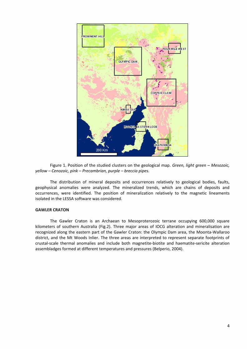
To confirm our conclusion about the ore controlling role of faults and fracture zones in the distribution of hypogenic deposits of Cu, Au, Ag, Pb, Fe, U, we analyzed the distribution of mineralization of different types and ages in different Geological Provinces of South Australia - GAWLER CRATON and ADELAIDE GEOSYNCLINE, where we analyzed clusters including deposits and ore occurrences of different types. The clusters are shown in Figure 1.

4

Figure 1. Position of the studied clusters on the geological map. Green, light green – Mesozoic,

yellow – Cenozoic, pink – Precambrian, purple – breccia pipes. The distribution of mineral deposits and occurrences relatively to geological bodies, faults,

geophysical anomalies were analyzed. The mineralized trends, which are chains of deposits and occurrences, were identified. The position of mineralization relatively to the magnetic lineaments isolated in the LESSA software was considered.

GAWLER CRATON

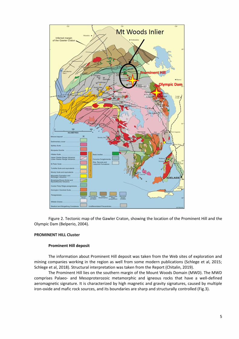
The Gawler Craton is an Archaean to Mesoproterozoic terrane occupying 600,000 square kilometers of southern Australia (Fig.2). Three major areas of IOCG alteration and mineralisation are recognized along the eastern part of the Gawler Craton: the Olympic Dam area, the Moonta-Wallaroo district, and the Mt Woods Inlier. The three areas are interpreted to represent separate footprints of crustal-scale thermal anomalies and include both magnetite-biotite and haematite-sericite alteration assembladges formed at different temperatures and pressures (Belperio, 2004).

5

Figure 2. Tectonic map of the Gawler Craton, showing the location of the Prominent Hill and the

Olympic Dam (Belperio, 2004).

PROMINENT HILL Cluster

Prominent Hill deposit The information about Prominent Hill deposit was taken from the Web sites of exploration and

mining companies working in the region as well from some modern publications (Schlege et al, 2015; Schlege et al, 2018). Structural interpretation was taken from the Report (Chitalin, 2019).

The Prominent Hill lies on the southern margin of the Mount Woods Domain (MWD). The MWD comprises Palaeo- and Mesoproterozoic metamorphic and igneous rocks that have a well-defined aeromagnetic signature. It is characterized by high magnetic and gravity signatures, caused by multiple iron-oxide and mafic rock sources, and its boundaries are sharp and structurally controlled (Fig.3).

6

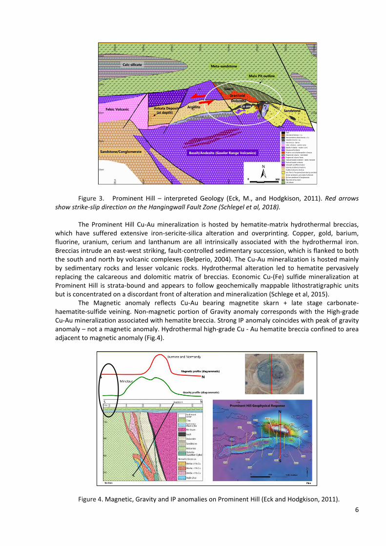
Figure 3. Prominent Hill – interpreted Geology (Eck, M., and Hodgkison, 2011). Red arrows show strike-slip direction on the Hangingwall Fault Zone (Schlegel et al, 2018).

The Prominent Hill Cu-Au mineralization is hosted by hematite-matrix hydrothermal breccias,

which have suffered extensive iron-sericite-silica alteration and overprinting. Copper, gold, barium, fluorine, uranium, cerium and lanthanum are all intrinsically associated with the hydrothermal iron. Breccias intrude an east-west striking, fault-controlled sedimentary succession, which is flanked to both the south and north by volcanic complexes (Belperio, 2004). The Cu-Au mineralization is hosted mainly by sedimentary rocks and lesser volcanic rocks. Hydrothermal alteration led to hematite pervasively replacing the calcareous and dolomitic matrix of breccias. Economic Cu-(Fe) sulfide mineralization at Prominent Hill is strata-bound and appears to follow geochemically mappable lithostratigraphic units but is concentrated on a discordant front of alteration and mineralization (Schlege et al, 2015).

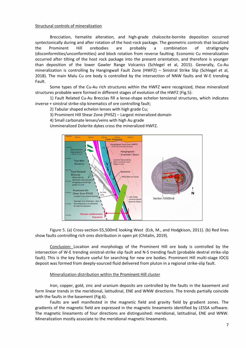
The Magnetic anomaly reflects Cu-Au bearing magnetite skarn + late stage carbonate-haematite-sulfide veining. Non-magnetic portion of Gravity anomaly corresponds with the High-grade Cu-Au mineralization associated with hematite breccia. Strong IP anomaly coincides with peak of gravity anomaly – not a magnetic anomaly. Hydrothermal high-grade Cu - Au hematite breccia confined to area adjacent to magnetic anomaly (Fig.4).

Figure 4. Magnetic, Gravity and IP anomalies on Prominent Hill (Eck and Hodgkison, 2011).

7

Structural controls of mineralization Brecciation, hematite alteration, and high-grade chalcocite-bornite deposition occurred

syntectonically during and after rotation of the host-rock package. The geometric controls that localized the Prominent Hill orebodies are probably a combination of stratigraphy (disconformities/unconformities) and block rotation from reverse faulting. Economic Cu mineralization occurred after tilting of the host rock package into the present orientation, and therefore is younger than deposition of the lower Gawler Range Volcanics (Schlegel et al, 2015). Generally, Cu-Au mineralization is controlling by Hangingwall Fault Zone (HWFZ) – Sinistral Strike Slip (Schlegel et al, 2018). The main Malu Cu ore body is controlled by the intersection of NNW faults and W-E trending Fault.

Some types of the Cu-Au rich structures within the HWFZ were recognized, these mineralized structures probable were formed in different stages of evolution of the HWFZ (Fig.5): 1) Fault Related Cu-Au Breccias fill a lense-shape echelon tensional structures, which indicates inverse + sinistral strike-slip kinematics of ore controlling fault; 2) Tabular shaped echelon lenses with high grade Cu; 3) Prominent Hill Shear Zone (PHSZ) – Largest mineralized domain 4) Small carbonate lenses/veins with high Au grade Unmineralized Dolerite dykes cross the mineralized HWFZ.

Figure 5. (a) Cross-section-55,500mE looking West (Eck, M., and Hodgkison, 2011). (b) Red lines show faults controlling rich ores distribution in open pit (Chitalin, 2019).

Conclusion: Location and morphology of the Prominent Hill ore body is controlled by the intersection of W-E trending sinistral-strike slip fault and N-S trending fault (probable dextral strike-slip fault). This is the key feature useful for searching for new ore bodies. Prominent Hill multi-stage IOCG deposit was formed from deeply-sourced fluid delivered from pluton in a regional strike-slip fault.

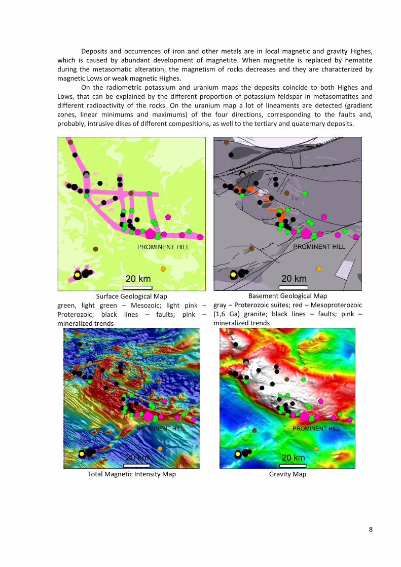
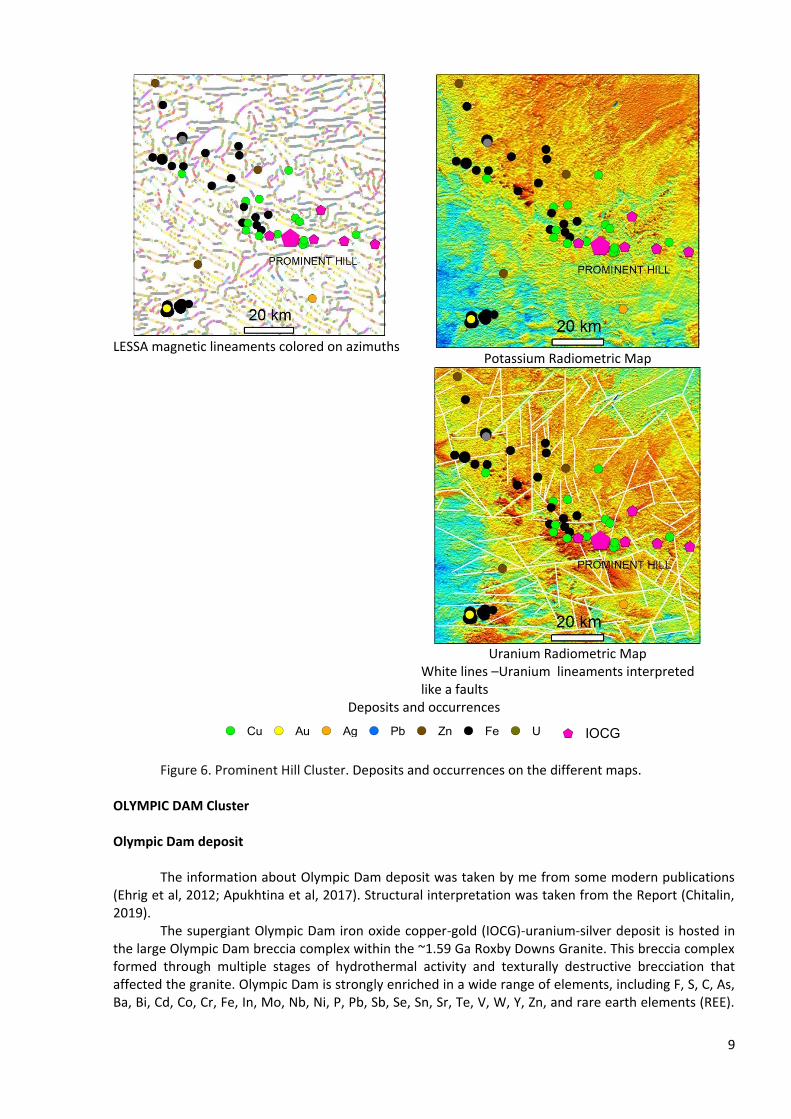
Mineralization distribution within the Prominent Hill cluster Iron, copper, gold, zinc and uranium deposits are controlled by the faults in the basement and

form linear trends in the meridional, latitudinal, ENE and WNW directions. The trends partially coincide with the faults in the basement (Fig.6).

Faults are well manifested in the magnetic field and gravity field by gradient zones. The gradients of the magnetic field are expressed in the magnetic lineaments identified by LESSA software. The magnetic lineaments of four directions are distinguished: meridional, latitudinal, ENE and WNW. Mineralization mostly associate to the meridional magnetic lineaments.

8

Deposits and occurrences of iron and other metals are in local magnetic and gravity Highes,

which is caused by abundant development of magnetite. When magnetite is replaced by hematite during the metasomatic alteration, the magnetism of rocks decreases and they are characterized by magnetic Lows or weak magnetic Highes.

On the radiometric potassium and uranium maps the deposits coincide to both Highes and Lows, that can be explained by the different proportion of potassium feldspar in metasomatites and different radioactivity of the rocks. On the uranium map a lot of lineaments are detected (gradient zones, linear minimums and maximums) of the four directions, corresponding to the faults and, probably, intrusive dikes of different compositions, as well to the tertiary and quaternary deposits.

Surface Geological Map

green, light green – Mesozoic; light pink – Proterozoic; black lines – faults; pink – mineralized trends

Basement Geological Map

gray – Proterozoic suites; red – Mesoproterozoic (1,6 Ga) granite; black lines – faults; pink – mineralized trends

Total Magnetic Intensity Map

Gravity Map

9

LESSA magnetic lineaments colored on azimuths

Potassium Radiometric Map

Uranium Radiometric Map

White lines –Uranium lineaments interpreted like a faults

Deposits and occurrences

Figure 6. Prominent Hill Cluster. Deposits and occurrences on the different maps. OLYMPIC DAM Cluster Olympic Dam deposit

The information about Olympic Dam deposit was taken by me from some modern publications

(Ehrig et al, 2012; Apukhtina et al, 2017). Structural interpretation was taken from the Report (Chitalin, 2019).

The supergiant Olympic Dam iron oxide copper-gold (IOCG)-uranium-silver deposit is hosted in the large Olympic Dam breccia complex within the ~1.59 Ga Roxby Downs Granite. This breccia complex formed through multiple stages of hydrothermal activity and texturally destructive brecciation that affected the granite. Olympic Dam is strongly enriched in a wide range of elements, including F, S, C, As, Ba, Bi, Cd, Co, Cr, Fe, In, Mo, Nb, Ni, P, Pb, Sb, Se, Sn, Sr, Te, V, W, Y, Zn, and rare earth elements (REE).

!( Cu !( Au !( Ag !( Pb !( Zn !( Fe !( U $+ IOCG

10

The deposit contains more than 90 minerals. The ore and gangue minerals are correlated with Fe abundance. There is a strong spatial association of Cu, U3O8, Au, and Ag (Ehrig et al, 2012).

A zircon U-Pb age for the felsic unit (1591 ± 11 Ma) implies that this unit is broadly coeval with the granite, whereas U-Pb ages for hydrothermal uraninite (1593.5 ± 5.1 Ma), Radiometric (1583.3 ± 6.5 Ma), and hematite (1592 ± 15 Ma) indicate that deposition of the U-REE–rich hydrothermal magnetite-fluorapatite-pyrite-quartz assemblage and replacement of magnetite by hematite occurred soon after emplacement of the granitic host rocks. Sm-Nd dating of ubiquitous calcite veins suggests formation at ~1.54 Ga (Apukhtina et al, 2017).

Structural control of mineralization

The structural interpretation completed by G.Dishaw is summarized below, based on the

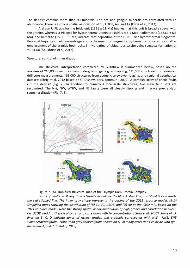
analyses of ~40,000 structures from underground geological mapping, ~21,000 structures from oriented drill core measurements, ~69,000 structures from acoustic televiewer logging, and regional geophysical datasets (Ehrig et al, 2012 based on G. Dishaw, pers. commun., 2009). A complex array of brittle faults cut the deposit (Fig. 7). In addition to numerous local-scale structures, five main fault sets are recognized. The N-S, NW, WNW, and NE faults were all steeply dipping and in place pre- and/or synmineralization (Fig. 7, 8).

Figure 7. (A) Simplified structural map of the Olympic Dam Breccia Complex. Limits of unaltered Roxby Downs Granite lie outside the blue dashed line, and >5 wt % Fe is inside

the red stippled line. The inner gray shape represents the outline of the 2011 resource model. (B-D) Simplified maps showing the distribution of (B) Cu, (C) U3O8, and (D) Au at the –350 mRL based on the 2011 resource model. Note the strong spatial linear distribution of high grades and correlation between Cu, U3O8, and Au. There is also a strong correlation with Fe concentration (Ehrig et al, 2012). Some black lines on B, C, D indicate zones of richest grades and probable corresponds with NW, NNE, ENE synmineralized faults. Note, than gray colored faults shown on A, in many cases don’t coincide with syn-mineralized faults! (Chitalin, 2019).

11

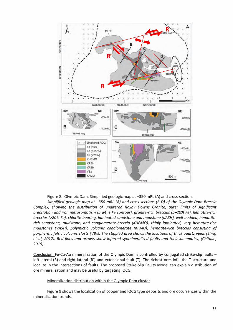
Figure 8. Olympic Dam. Simplified geologic map at –350 mRL (A) and cross-sections. Simplified geologic map at –350 mRL (A) and cross-sections (B-D) of the Olympic Dam Breccia

Complex, showing the distribution of unaltered Roxby Downs Granite, outer limits of significant brecciation and iron metasomatism (5 wt % Fe contour), granite-rich breccias (5–20% Fe), hematite-rich breccias (>20% Fe), chlorite-bearing, laminated sandstone and mudstone (KASH), well-bedded, hematite-rich sandstone, mudstone, and conglomerate-breccia (KHEMQ), thinly laminated, very hematite-rich mudstones (VASH), polymictic volcanic conglomerate (KFMU), hematite-rich breccias consisting of porphyritic felsic volcanic clasts (VBx). The stippled area shows the locations of thick quartz veins (Ehrig et al, 2012). Red lines and arrows show inferred synmineralized faults and their kinematics, (Chitalin, 2019).

Conclusion: Fe-Cu-Au mineralization of the Olympic Dam is controlled by conjugated strike-slip faults – left-lateral (R) and right-lateral (R’) and extensional fault (T). The richest ores infill the T-structure and localize in the intersections of faults. The proposed Strike-Slip Faults Model can explain distribution of ore mineralization and may be useful by targeting IOCG.

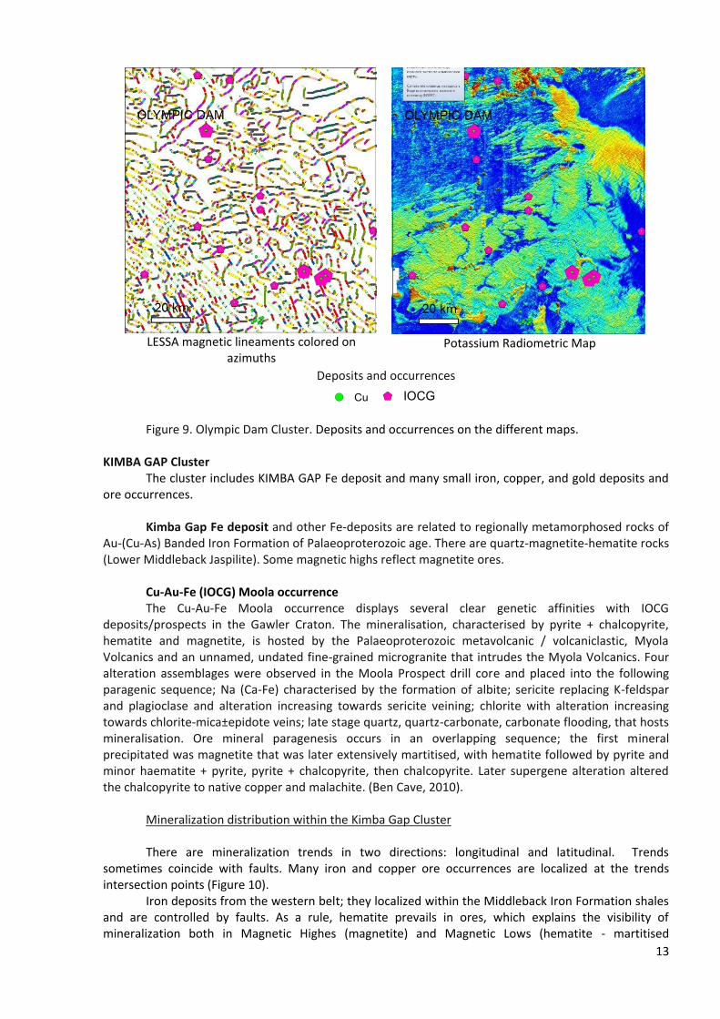
Mineralization distribution within the Olympic Dam cluster Figure 9 shows the localization of copper and IOCG type deposits and ore occurrences within the

mineralization trends.

12

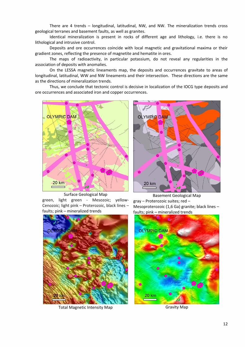
There are 4 trends – longitudinal, latitudinal, NW, and NW. The mineralization trends cross geological terranes and basement faults, as well as granites.

Identical mineralization is present in rocks of different age and lithology, i.e. there is no lithological and intrusive control.

Deposits and ore occurrences coincide with local magnetic and gravitational maxima or their gradient zones, reflecting the presence of magnetite and hematite in ores.

The maps of radioactivity, in particular potassium, do not reveal any regularities in the association of deposits with anomalies.

On the LESSA magnetic lineaments map, the deposits and occurrences gravitate to areas of longitudinal, latitudinal, WW and NW lineaments and their intersection. These directions are the same as the directions of mineralization trends.

Thus, we conclude that tectonic control is decisive in localization of the IOCG type deposits and ore occurrences and associated iron and copper occurrences.


green, light green - Mesozoic; yellow-Cenozoic; light pink – Proterozoic, black lines – faults; pink – mineralized trends


gray – Proterozoic suites; red – Mesoproterozoic (1,6 Ga) granite; black lines – faults; pink – mineralized trends


Gravity Map

13

LESSA magnetic lineaments colored on

azimuths



Figure 9. Olympic Dam Cluster. Deposits and occurrences on the different maps. KIMBA GAP Cluster

The cluster includes KIMBA GAP Fe deposit and many small iron, copper, and gold deposits and ore occurrences.

Kimba Gap Fe deposit and other Fe-deposits are related to regionally metamorphosed rocks of

Au-(Cu-As) Banded Iron Formation of Palaeoproterozoic age. There are quartz-magnetite-hematite rocks (Lower Middleback Jaspilite). Some magnetic highs reflect magnetite ores.

Cu-Au-Fe (IOCG) Moola occurrence The Cu-Au-Fe Moola occurrence displays several clear genetic affinities with IOCG

deposits/prospects in the Gawler Craton. The mineralisation, characterised by pyrite + chalcopyrite, hematite and magnetite, is hosted by the Palaeoproterozoic metavolcanic / volcaniclastic, Myola Volcanics and an unnamed, undated fine-grained microgranite that intrudes the Myola Volcanics. Four alteration assemblages were observed in the Moola Prospect drill core and placed into the following paragenic sequence; Na (Ca-Fe) characterised by the formation of albite; sericite replacing K-feldspar and plagioclase and alteration increasing towards sericite veining; chlorite with alteration increasing towards chlorite-mica±epidote veins; late stage quartz, quartz-carbonate, carbonate flooding, that hosts mineralisation. Ore mineral paragenesis occurs in an overlapping sequence; the first mineral precipitated was magnetite that was later extensively martitised, with hematite followed by pyrite and minor haematite + pyrite, pyrite + chalcopyrite, then chalcopyrite. Later supergene alteration altered the chalcopyrite to native copper and malachite. (Ben Cave, 2010).

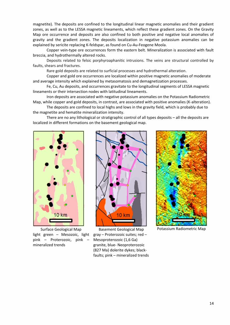
Mineralization distribution within the Kimba Gap Cluster There are mineralization trends in two directions: longitudinal and latitudinal. Trends

sometimes coincide with faults. Many iron and copper ore occurrences are localized at the trends intersection points (Figure 10).

Iron deposits from the western belt; they localized within the Middleback Iron Formation shales and are controlled by faults. As a rule, hematite prevails in ores, which explains the visibility of mineralization both in Magnetic Highes (magnetite) and Magnetic Lows (hematite - martitised

!( Cu $+ IOCG

14

magnetite). The deposits are confined to the longitudinal linear magnetic anomalies and their gradient zones, as well as to the LESSA magnetic lineaments, which reflect these gradient zones. On the Gravity Map ore occurrence and deposits are also confined to both positive and negative local anomalies of gravity and the gradient zones. The deposits localization in negative potassium anomalies can be explained by sericite replacing K-feldspar, as found on Cu-Au-Feogene Moola.

Copper vein-type ore occurrences form the eastern belt. Mineralization is associated with fault breccia, and hydrothermally altered rocks.

Deposits related to felsic porphyroaphanitic intrusions. The veins are structural controlled by faults, shears and fractures.

Rare gold deposits are related to surficial processes and hydrothermal alteration. Copper and gold ore occurrences are localized within positive magnetic anomalies of moderate

and average intensity which explained by metasomatosis and demagnetization processes. Fe, Cu, Au deposits, and occurrences gravitate to the longitudinal segments of LESSA magnetic

lineaments or their intersection nodes with latitudinal lineaments. Iron deposits are associated with negative potassium anomalies on the Potassium Radiometric

Map, while copper and gold deposits, in contrast, are associated with positive anomalies (K-alteration). The deposits are confined to local highs and lows in the gravity field, which is probably due to

the magnetite and hematite mineralization intensity. There are no any lithological or stratigraphic control of all types deposits – all the deposits are

localized in different formations on the basement geological map.


light green – Mesozoic, light pink – Proterozoic, pink – mineralized trends

Basement Geological Map gray – Proterozoic suites; red – Mesoproterozoic (1,6 Ga) granite, blue- Neoproterozoic (827 Ma) dolerite dykes; black-faults; pink – mineralized trends


15


LESSA magnetic lineaments

colored on azimuthes

Gravity Map


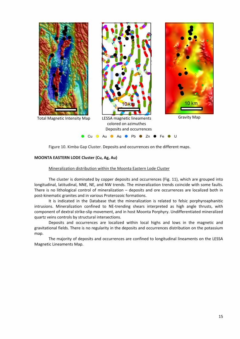
Figure 10. Kimba Gap Cluster. Deposits and occurrences on the different maps. MOONTA EASTERN LODE Cluster (Cu, Ag, Au)

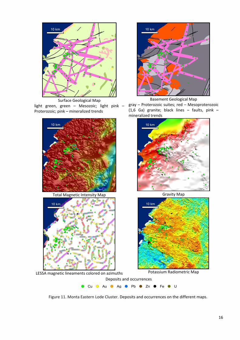
Mineralization distribution within the Moonta Eastern Lode Cluster The cluster is dominated by copper deposits and occurrences (Fig. 11), which are grouped into

longitudinal, latitudinal, NNE, NE, and NW trends. The mineralization trends coincide with some faults. There is no lithological control of mineralization – deposits and ore occurrences are localized both in post-kinematic granites and in various Proterozoic formations.

It is indicated in the Database that the mineralization is related to felsic porphyroaphanitic intrusions. Mineralization confined to NE-trending shears interpreted as high angle thrusts, with component of dextral strike-slip movement, and in host Moonta Porphyry. Undifferentiated mineralized quartz veins controls by structural intersections.

Deposits and occurrences are localized within local highs and lows in the magnetic and gravitational fields. There is no regularity in the deposits and occurrences distribution on the potassium map.

The majority of deposits and occurrences are confined to longitudinal lineaments on the LESSA Magnetic Lineaments Map.

!( Cu !( Au !( Ag !( Pb !( Zn !( Fe !( U

16


light green, green – Mesozoic; light pink – Proterozoic; pink – mineralized trends


gray – Proterozoic suites; red – Mesoproterozoic (1,6 Ga) granite; black lines – faults, pink – mineralized trends


Gravity Map




Figure 11. Monta Eastern Lode Cluster. Deposits and occurrences on the different maps.

!( Cu !( Au !( Ag !( Pb !( Zn !( Fe !( U

17

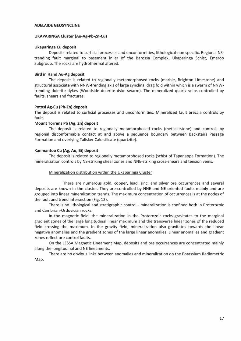
ADELAIDE GEOSYNCLINE UKAPARINGA Cluster (Au-Ag-Pb-Zn-Cu) Ukaparinga Cu deposit

Deposits related to surficial processes and unconformities, lithological-non specific. Regional NS-trending fault marginal to basement inlier of the Barossa Complex, Ukaparinga Schist, Emeroo Subgroup. The rocks are hydrothermal altered.

Bird in Hand Au-Ag deposit

The deposit is related to regionally metamorphosed rocks (marble, Brighton Limestone) and structural associate with NNW-trending axis of large synclinal drag fold within which is a swarm of NNW-trending dolerite dykes (Woodside dolerite dyke swarm). The mineralized quartz veins controlled by faults, shears and fractures.

Potosi Ag-Cu (Pb-Zn) deposit The deposit is related to surficial processes and unconformities. Mineralized fault breccia controls by fault. Mount Torrens Pb (Ag, Zn) deposit

The deposit is related to regionally metamorphosed rocks (metasiltstone) and controls by regional disconformable contact at and above a sequence boundary between Backstairs Passage Formation and overlying Talisker Calc-silicate (quartzite).

Kanmantoo Cu (Ag, Au, Bi) deposit

The deposit is related to regionally metamorphosed rocks (schist of Tapanappa Formation). The mineralization controls by NS-striking shear zones and NNE-striking cross-shears and tension veins.

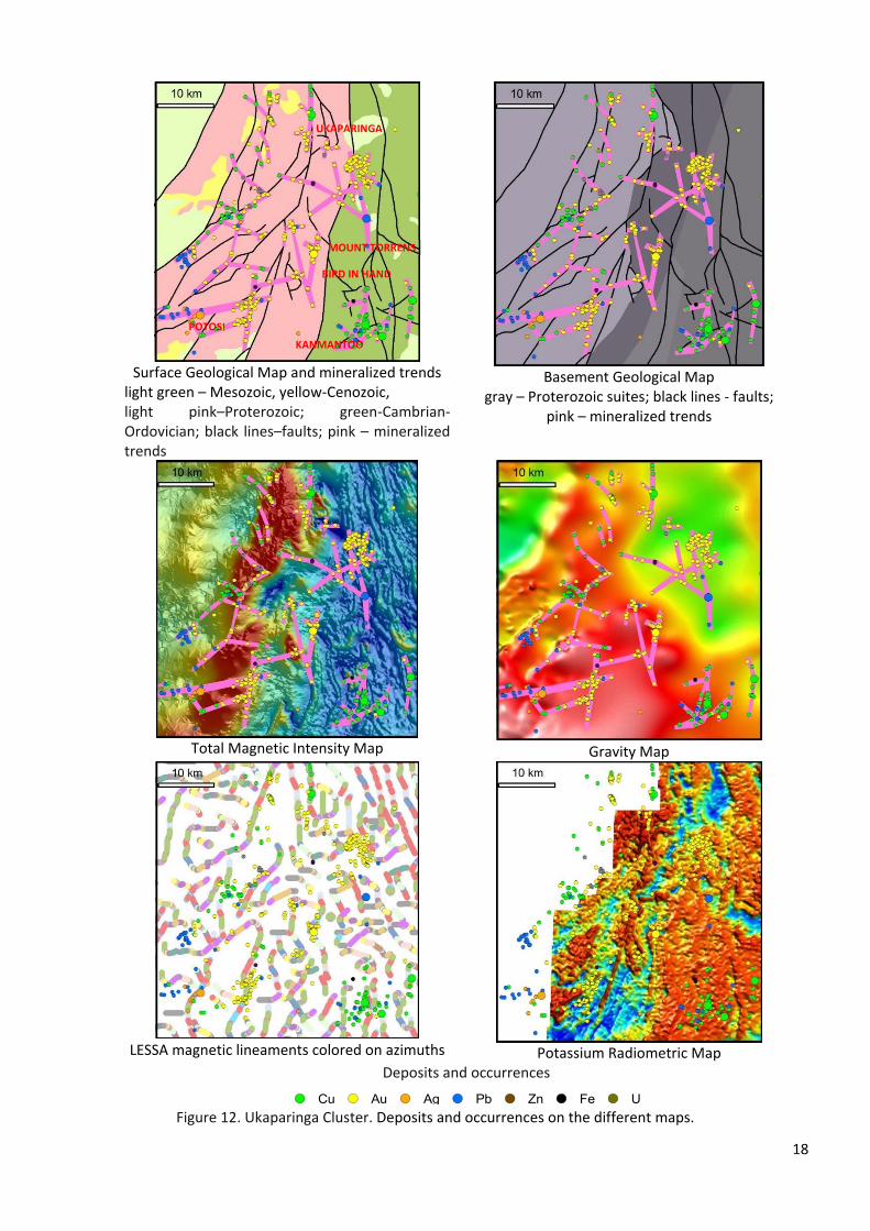
Mineralization distribution within the Ukaparinga Cluster There are numerous gold, copper, lead, zinc, and silver ore occurrences and several

deposits are known in the cluster. They are controlled by NNE and NE oriented faults mainly and are grouped into linear mineralization trends. The maximum concentration of occurrences is at the nodes of the fault and trend intersection (Fig. 12).

There is no lithological and stratigraphic control - mineralization is confined both in Proterozoic and Cambrian-Ordovician rocks.

In the magnetic field, the mineralization in the Proterozoic rocks gravitates to the marginal gradient zones of the large longitudinal linear maximum and the transverse linear zones of the reduced field crossing the maximum. In the gravity field, mineralization also gravitates towards the linear negative anomalies and the gradient zones of the large linear anomalies. Linear anomalies and gradient zones reflect ore control faults.

On the LESSA Magnetic Lineament Map, deposits and ore occurrences are concentrated mainly along the longitudinal and NE lineaments.

There are no obvious links between anomalies and mineralization on the Potassium Radiometric Map.

18

Surface Geological Map and mineralized trends

light green – Mesozoic, yellow-Cenozoic, light pink–Proterozoic; green-Cambrian-Ordovician; black lines–faults; pink – mineralized trends


gray – Proterozoic suites; black lines - faults; pink – mineralized trends


Gravity Map




Figure 12. Ukaparinga Cluster. Deposits and occurrences on the different maps.

!( Cu !( Au !( Ag !( Pb !( Zn !( Fe !( U

UKAPARINGA

BIRD IN HAND

POTOSI

MOUNT TORRENS

KANMANTOO

19

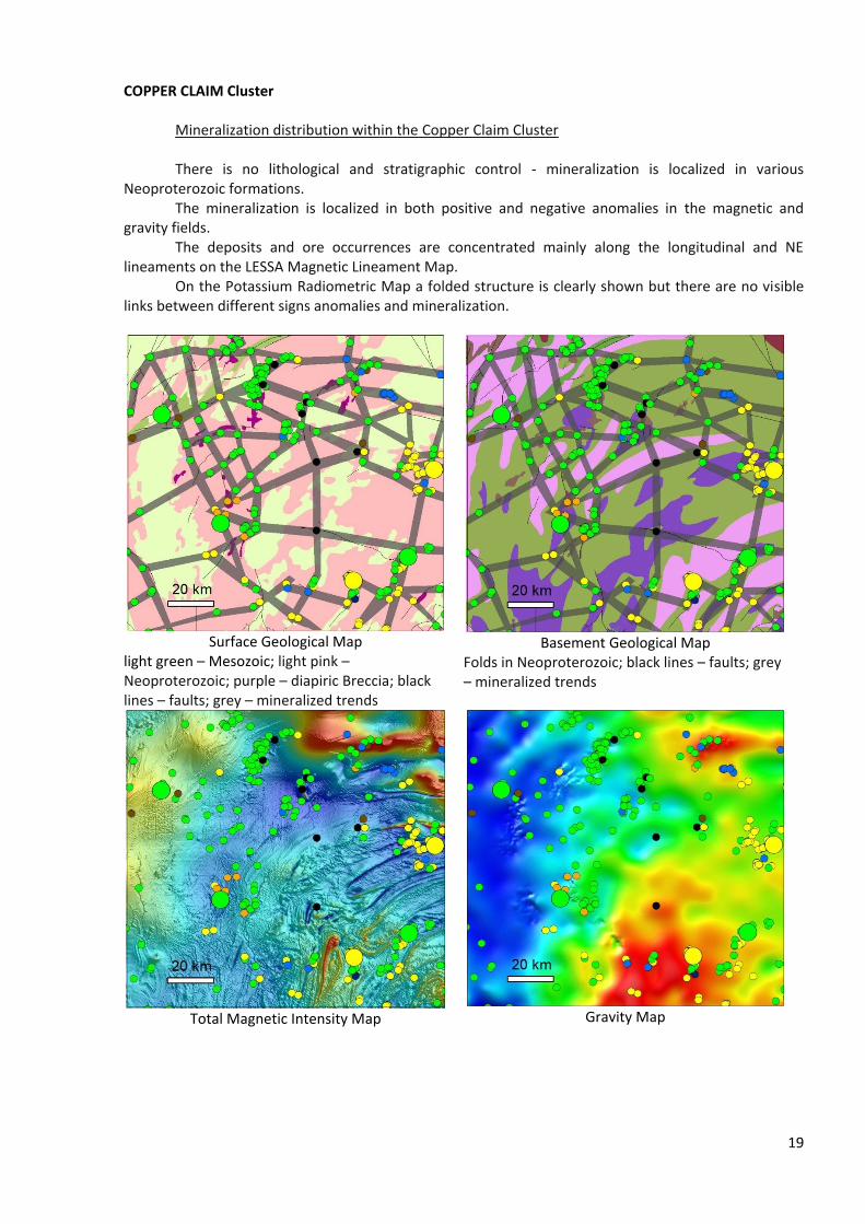
COPPER CLAIM Cluster

Mineralization distribution within the Copper Claim Cluster

There is no lithological and stratigraphic control - mineralization is localized in various Neoproterozoic formations.

The mineralization is localized in both positive and negative anomalies in the magnetic and gravity fields.

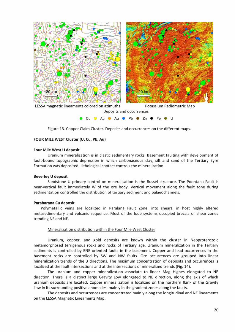
The deposits and ore occurrences are concentrated mainly along the longitudinal and NE lineaments on the LESSA Magnetic Lineament Map.

On the Potassium Radiometric Map a folded structure is clearly shown but there are no visible links between different signs anomalies and mineralization.


light green – Mesozoic; light pink – Neoproterozoic; purple – diapiric Breccia; black lines – faults; grey – mineralized trends


Folds in Neoproterozoic; black lines – faults; grey – mineralized trends


Gravity Map

20




Figure 13. Copper Claim Cluster. Deposits and occurrences on the different maps. FOUR MILE WEST Cluster (U, Cu, Pb, Au) Four Mile West U deposit

Uranium mineralization is in clastic sedimentary rocks. Basement faulting with development of fault-bound topographic depression in which carbonaceous clay, silt and sand of the Tertiary Eyre Formation was deposited. Lithological contact controls the mineralization.

Beverley U deposit

Sandstone U primary control on mineralisation is the Russel structure. The Poontana Fault is near-vertical fault immediately W of the ore body. Vertical movement along the fault zone during sedimentation controlled the distribution of tertiary sediment and palaeochannels.

Parabarana Cu deposit

Polymetallic veins are localized in Paralana Fault Zone, into shears, in host highly altered metasedimentary and volcanic sequence. Most of the lode systems occupied breccia or shear zones trending NS and NE.

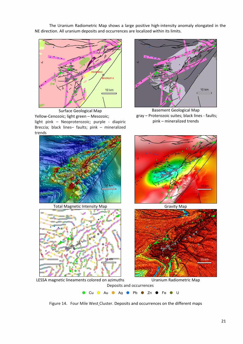
Mineralization distribution within the Four Mile West Cluster Uranium, copper, and gold deposits are known within the cluster in Neoproterozoic

metamorphosed terrigenous rocks and rocks of Tertiary age. Uranium mineralization in the Tertiary sediments is controlled by ENE oriented faults in the basement. Copper and lead occurrences in the basement rocks are controlled by SW and NW faults. Ore occurrences are grouped into linear mineralization trends of the 3 directions. The maximum concentration of deposits and occurrences is localized at the fault intersections and at the intersections of mineralized trends (Fig. 14).

The uranium and copper mineralization associate to linear Mag Highes elongated to NE direction. There is a distinct large Gravity Low elongated to NE direction, along the axis of which uranium deposits are located. Copper mineralization is localized on the northern flank of the Gravity Low in its surrounding positive anomalies, mainly in the gradient zones along the faults.

The deposits and occurrences are concentrated mainly along the longitudinal and NE lineaments on the LESSA Magnetic Lineaments Map.

!( Cu !( Au !( Ag !( Pb !( Zn !( Fe !( U

21

The Uranium Radiometric Map shows a large positive high-intensity anomaly elongated in the NE direction. All uranium deposits and occurrences are localized within its limits.


Yellow-Cenozoic; light green – Mesozoic; light pink – Neoproterozoic; purple - diapiric Breccia; black lines– faults; pink – mineralized trends


gray – Proterozoic suites; black lines - faults; pink – mineralized trends


Gravity Map


Uranium Radiometric Map


Figure 14. Four Mile West Cluster. Deposits and occurrences on the different maps

!( Cu !( Au !( Ag !( Pb !( Zn !( Fe !( U

FOUR MILE

BEVERLEY U

PARABARANA

22

Conclusions: The examined examples of various types and ages mineralization in different geological provinces

allow drawing the following conclusions: Deposits and occurrences are controlled by faults and structural mineralization trends (fracture and

permeability zones). The maximum concentration of mineralization is localized at the intersection points of faults and

structural mineralization trends. The stratigraphic and lithological control of mineralization localization is subordinate or absent. The mineralization is associated with both local maxima (magnetite) and minima (metasomatic

alteration, demagnetization, fault zones) in the magnetic and gravity field. There are four main directions on the magnetic lineament maps: longitudinal, latitudinal, NW, NE,

with which the occurrences and fields are linked. There are longitudinal ore control structures that prevail.

The deposits may both be associated with local positive and negative anomalies, and do not detect any visible links with the anomalies on the maps of Radiometric potassium and uranium. The localization of uranium and uranium-containing copper deposits and occurrences are visible by positive anomalies of varying intensity on the Radiometric Uranium map. These anomalies are often linear and reflect ore control faults within the basement.

The considered features of deposits and occurrences are reflected indirectly on geological and geophysical maps, which we used for machine learning and deposits forecasting processes.

Useful Maps for Machine Learning As all the considered ore occurrences and deposits are hydrothermal and associated with faults, all

of them have many similar signs of structural control, metasomatic changes, and mineralization, which are reflected in geophysical fields. The geological and geophysical maps which reflect the main features of deposits and ore occurrences have been used for machine learning algorithm. The raster has a resolution of 2000 pixels. A geological map of pre-Mesozoic formations has been created to take into account all the geological bodies containing deposits and ore occurrences (stratigraphic subdivisions, lithological varieties of rocks, intrusive formations). The list of maps is given in the table. Our solution uses data from 8 regional maps (rasters) for the whole of South Australia, listed in Table 1.

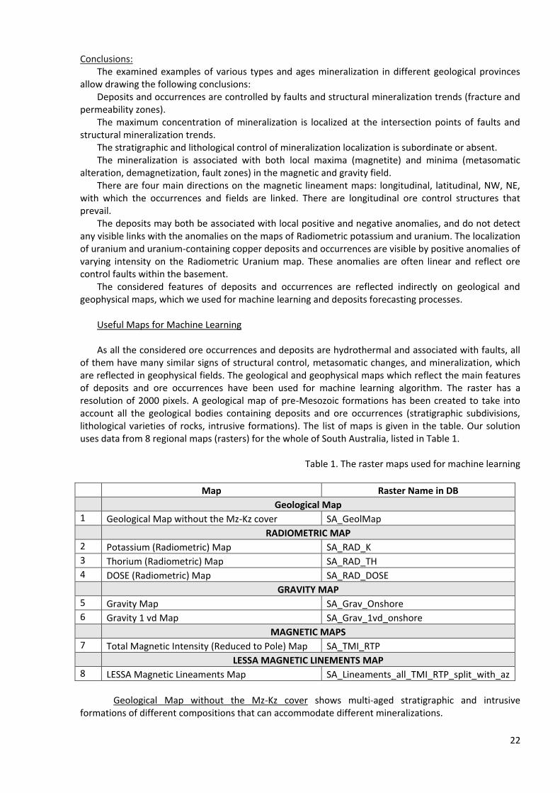
Table 1. The raster maps used for machine learning

Map Raster Name in DB Geological Map

1 Geological Map without the Mz-Kz cover SA_GeolMap RADIOMETRIC MAP

2 Potassium (Radiometric) Map SA_RAD_K 3 Thorium (Radiometric) Map SA_RAD_TH 4 DOSE (Radiometric) Map SA_RAD_DOSE

GRAVITY MAP 5 Gravity Map SA_Grav_Onshore 6 Gravity 1 vd Map SA_Grav_1vd_onshore

MAGNETIC MAPS 7 Total Magnetic Intensity (Reduced to Pole) Map SA_TMI_RTP

LESSA MAGNETIC LINEMENTS MAP 8 LESSA Magnetic Lineaments Map SA_Lineaments_all_TMI_RTP_split_with_az

Geological Map without the Mz-Kz cover shows multi-aged stratigraphic and intrusive formations of different compositions that can accommodate different mineralizations.

23

Radiometric maps: Potassium anomalies reflect alkaline granitoids, areas of metasomatic potassium alteration, which may be associated with mineralization. Thorium and DOSE anomalies reflect uranium and REE mineralization. They are associated with uranium deposits of different types and ages, as well as with the associated uranium mineralization at IOCG (Olympic Dam) type deposits.

Geophysical Maps: Gravity Map - Gravity Highes reflect high-density rocks and ores: magnetite and hematite ores, massive sulfides, mafic intrusions with copper-nickel, and PGE mineralization. Gravity 1 vd Map - anomalies reflect faults and contrast lithology rock boundaries that can control ore mineralization localization. Total Magnetic Intensity reduced to Pole Map - Mag Highes reflect magnetite ores and mafic rocks. Mag Lows can be caused by granites and also reflect near-ore metasomatic alteration and demagnetization areas and zones.

Scale used: the above raster maps are created in 1:7,000,000 scale and presented as high-resolution color images (23375x16542px). Each of them represents a geological or physical characteristic.

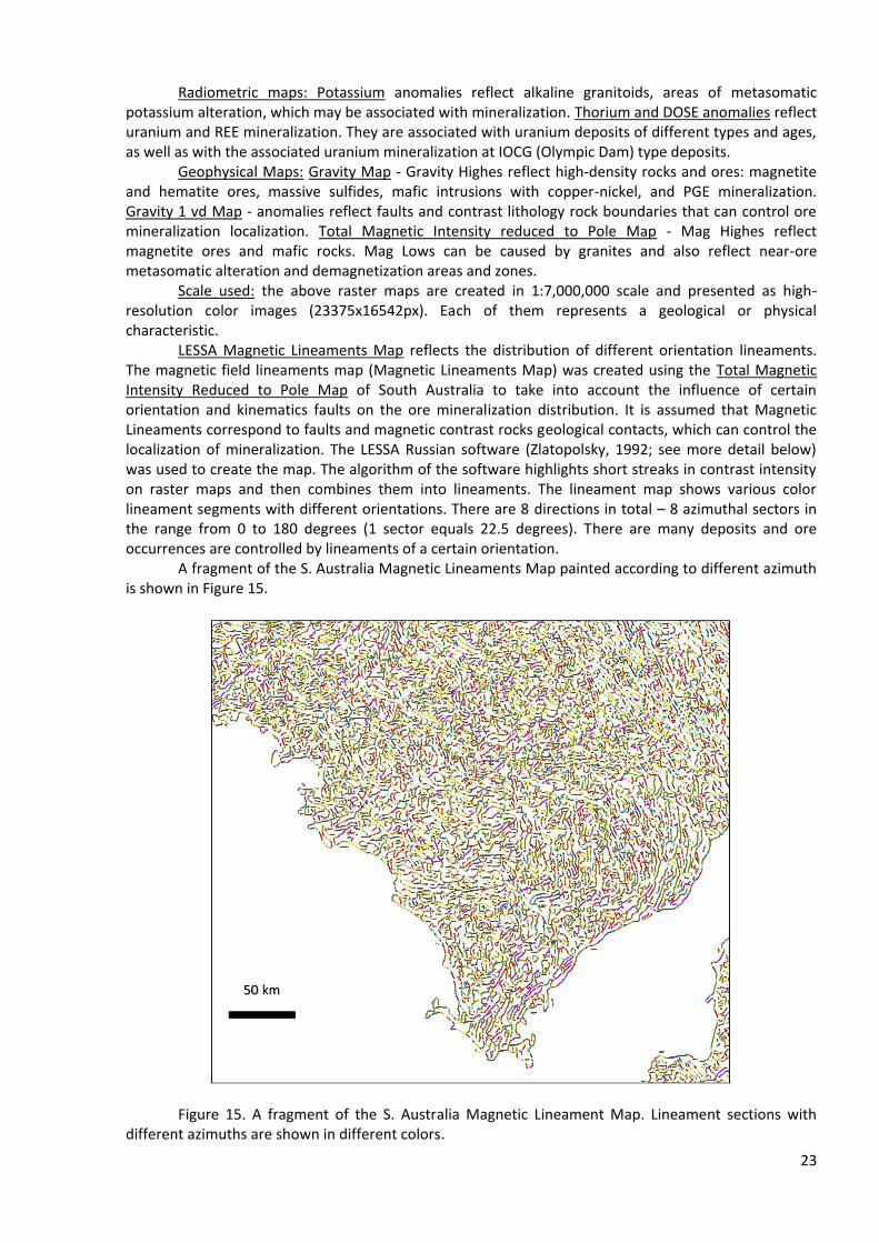
LESSA Magnetic Lineaments Map reflects the distribution of different orientation lineaments. The magnetic field lineaments map (Magnetic Lineaments Map) was created using the Total Magnetic Intensity Reduced to Pole Map of South Australia to take into account the influence of certain orientation and kinematics faults on the ore mineralization distribution. It is assumed that Magnetic Lineaments correspond to faults and magnetic contrast rocks geological contacts, which can control the localization of mineralization. The LESSA Russian software (Zlatopolsky, 1992; see more detail below) was used to create the map. The algorithm of the software highlights short streaks in contrast intensity on raster maps and then combines them into lineaments. The lineament map shows various color lineament segments with different orientations. There are 8 directions in total – 8 azimuthal sectors in the range from 0 to 180 degrees (1 sector equals 22.5 degrees). There are many deposits and ore occurrences are controlled by lineaments of a certain orientation.

A fragment of the S. Australia Magnetic Lineaments Map painted according to different azimuth is shown in Figure 15.

Figure 15. A fragment of the S. Australia Magnetic Lineament Map. Lineament sections with different azimuths are shown in different colors.

24

About LESSA (Zlatopolsky, 1992): The LESSA software - Lineament Extraction and Stripe Statistical Analysis - automatically extracts linear image features and analyzes their orientation and spatial distribution. LESSA provides picture (texture) description in the way common for the geological research: rose-diagrams, densities of features with a certain orientation, schemes of long lineaments, and several new descriptors of the rose-diagram features are also provided: vectors and lines of elongation, local rose diagrams difference, and the others. LESSA methods could be applied to different types of data - gray tone image, binary schemes (drainage network, for example), digital terrain map (DTM) - giving territory description in a common way. The proposed algorithm is based on the linear image features analysis (so-called "stripes"). LESSA automatically detects stripes and determines their direction (16 directions). The stripes detected at the first step are combined into the straight lines – lineaments).

The maps of deposits and ore occurrences which are grouped by classes of main metals in ores (main commodity) were also created for machine learning purposes. The deposits and ore occurrences are shown on the maps with black circles of the same size. The diameter of the circles is approximately 720 m on the ground (area 0.5 sq. km). The selected circles' size does not exceed the average deposit size - usually small and medium-sized deposits have an area of no more than 1 sq. km. 2.2.2 Deposits to Machine Learning

The database of different type deposits and ore occurrences was analyzed to select the forecasting purposes (Table 2). As follows from the table, the following metals hypogenic deposits and occurrences prevail quantitatively, in descending order: Cu (1337), Au (994), Pb-Zn (267), U (188).

The analysis results showed that different types of same metal deposits or complex deposits are controlled by faults and tectonic fracture zones. Stratigraphic and lithological control are of subordinate importance but are taken into account during machine learning indirectly through the mineralization points position on the basement geological map, where different stratigraphic subdivisions and intrusive formations of different ages are shown with various colors.

The different type deposits of the same metal are often controlled by the same faults and form the same mineralization trends. That is why for machine learning purposes it is not expedient to provide separate training by types of deposits, besides for effective training it is necessary to provide a rather representative sample (not less than 100-200 objects of one class). Therefore, all deposits and occurrences of different types are grouped by metals.

The machine learning process also took into account Mesozoic (?) and Tertiary stratiform deposits of uranium, copper, and polymetals, located in the sedimentary cover, but which are also controlled by basement faults. Their number is relatively small.

There are no magmatic deposits of platinoids, copper, and nickel, as well as alluvial deposits of gold and platinoids, were involved in the machine learning process.

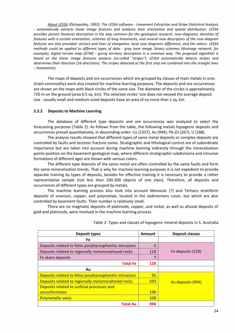
Table 2: Types and classes of hypogenic mineral deposits in S. Australia

Deposit types Amount Deposit classes

Fe Deposits related to felsic porphyroaphanitic intrusions 4

Fe deposits (129) Deposits related to regionally metamorphosed rocks 118 Fe skarn deposits 7

Total Fe 129 Au

Deposits related to felsic porphyroaphanitic intrusions 95 Au deposits (994)

Deposits related to regionally metamorphosed rocks 593 Deposits related to surficial processes and unconformities 198 Polymetallic veins 108

Total Au 994

25

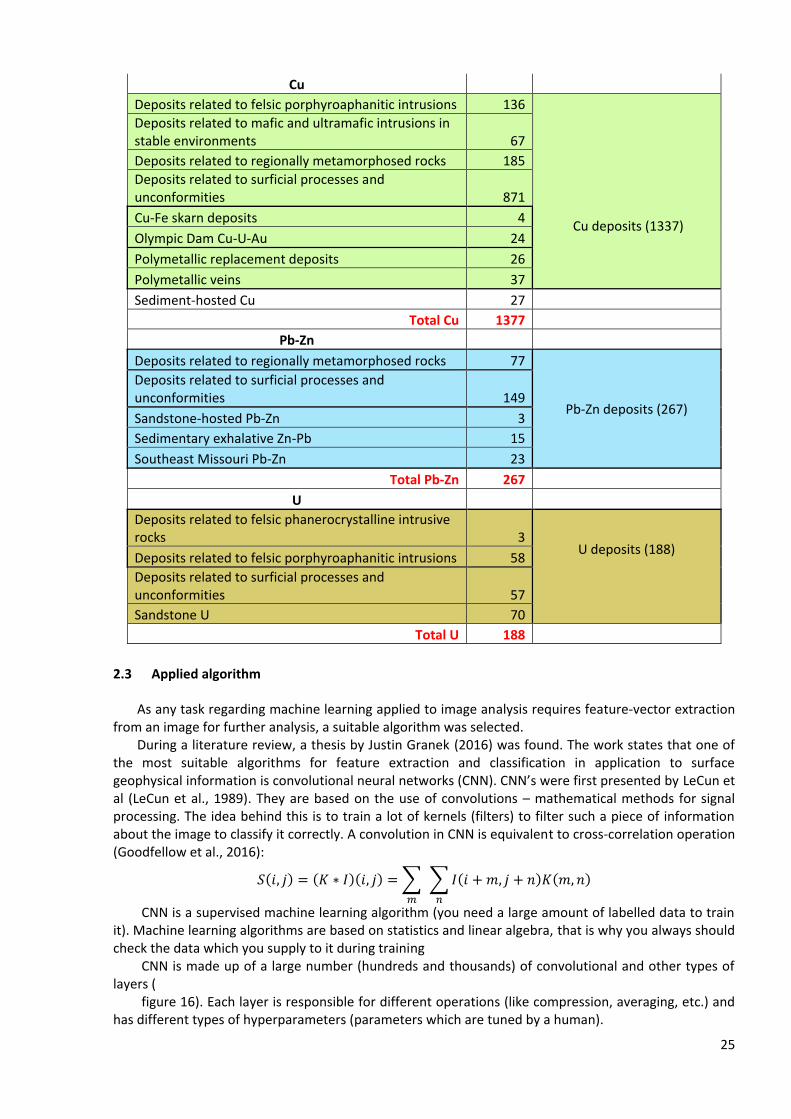
Cu Deposits related to felsic porphyroaphanitic intrusions 136

Cu deposits (1337)

Deposits related to mafic and ultramafic intrusions in stable environments 67 Deposits related to regionally metamorphosed rocks 185 Deposits related to surficial processes and unconformities 871 Cu-Fe skarn deposits 4 Olympic Dam Cu-U-Au 24 Polymetallic replacement deposits 26 Polymetallic veins 37 Sediment-hosted Cu 27

Total Cu 1377 Pb-Zn

Deposits related to regionally metamorphosed rocks 77

Pb-Zn deposits (267)

Deposits related to surficial processes and unconformities 149 Sandstone-hosted Pb-Zn 3 Sedimentary exhalative Zn-Pb 15 Southeast Missouri Pb-Zn 23

Total Pb-Zn 267 U

Deposits related to felsic phanerocrystalline intrusive rocks 3

U deposits (188)

Deposits related to felsic porphyroaphanitic intrusions 58 Deposits related to surficial processes and unconformities 57 Sandstone U 70

Total U 188 2.3 Applied algorithm

As any task regarding machine learning applied to image analysis requires feature-vector extraction from an image for further analysis, a suitable algorithm was selected.

During a literature review, a thesis by Justin Granek (2016) was found. The work states that one of the most suitable algorithms for feature extraction and classification in application to surface geophysical information is convolutional neural networks (CNN). CNN’s were first presented by LeCun et al (LeCun et al., 1989). They are based on the use of convolutions – mathematical methods for signal processing. The idea behind this is to train a lot of kernels (filters) to filter such a piece of information about the image to classify it correctly. A convolution in CNN is equivalent to cross-correlation operation (Goodfellow et al., 2016):

( , ) = ( ∗ )( , ) = ( + , + ) ( , )

CNN is a supervised machine learning algorithm (you need a large amount of labelled data to train it). Machine learning algorithms are based on statistics and linear algebra, that is why you always should check the data which you supply to it during training

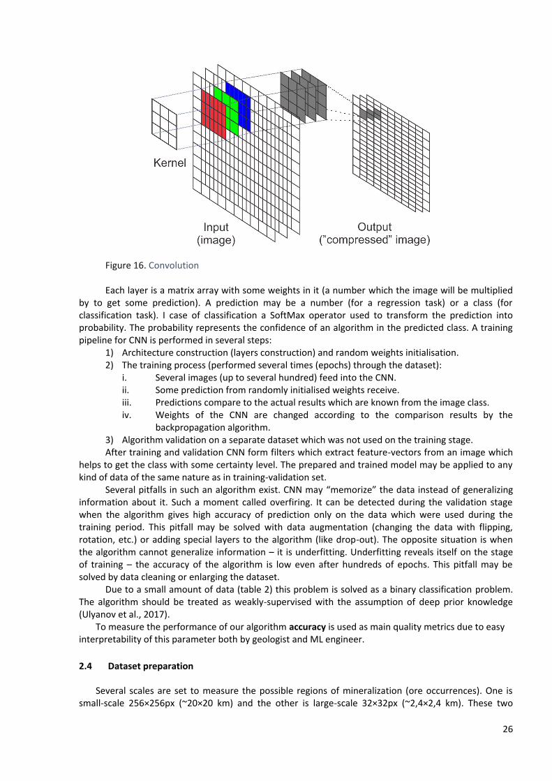
CNN is made up of a large number (hundreds and thousands) of convolutional and other types of layers (

figure 16). Each layer is responsible for different operations (like compression, averaging, etc.) and has different types of hyperparameters (parameters which are tuned by a human).

26

Figure 16. Convolution

Each layer is a matrix array with some weights in it (a number which the image will be multiplied

by to get some prediction). A prediction may be a number (for a regression task) or a class (for classification task). I case of classification a SoftMax operator used to transform the prediction into probability. The probability represents the confidence of an algorithm in the predicted class. A training pipeline for CNN is performed in several steps:

1) Architecture construction (layers construction) and random weights initialisation. 2) The training process (performed several times (epochs) through the dataset):

i. Several images (up to several hundred) feed into the CNN. ii. Some prediction from randomly initialised weights receive. iii. Predictions compare to the actual results which are known from the image class. iv. Weights of the CNN are changed according to the comparison results by the

backpropagation algorithm. 3) Algorithm validation on a separate dataset which was not used on the training stage. After training and validation CNN form filters which extract feature-vectors from an image which

helps to get the class with some certainty level. The prepared and trained model may be applied to any kind of data of the same nature as in training-validation set.

Several pitfalls in such an algorithm exist. CNN may “memorize” the data instead of generalizing information about it. Such a moment called overfiring. It can be detected during the validation stage when the algorithm gives high accuracy of prediction only on the data which were used during the training period. This pitfall may be solved with data augmentation (changing the data with flipping, rotation, etc.) or adding special layers to the algorithm (like drop-out). The opposite situation is when the algorithm cannot generalize information – it is underfitting. Underfitting reveals itself on the stage of training – the accuracy of the algorithm is low even after hundreds of epochs. This pitfall may be solved by data cleaning or enlarging the dataset.

Due to a small amount of data (table 2) this problem is solved as a binary classification problem. The algorithm should be treated as weakly-supervised with the assumption of deep prior knowledge (Ulyanov et al., 2017).

To measure the performance of our algorithm accuracy is used as main quality metrics due to easy interpretability of this parameter both by geologist and ML engineer.

2.4 Dataset preparation

Several scales are set to measure the possible regions of mineralization (ore occurrences). One is small-scale 256×256px (~20×20 km) and the other is large-scale 32×32px (~2,4×2,4 km). These two

27

scales were chosen as primary for regional-scale and local-scale mineralization search. Eight geophysical maps were cropped to tiles of chosen scale.

Six datasets were formed from the tiles. One for any mineralization class (2955 points) and one for each separate mineralization class (table 2). Due to the lack of data each separate dataset unites all types of deposit for each class. These tiles were marked as “deposit” class. To create a “no-deposit” class images were selected from the other part of the dataset which are not presented in the first class.

They were separated into two classes: with mineralization and without it. Areas with known mineralization were taken. After data preparation 447 (3809 for eight maps and total 7456 with randomly selected “no-deposit” class) tiles for all mineralization gained, 171 for Au (1367, 5031), 292 for Cu (2332, 4396), 106 for Fe (848, 1680), 113 for Pb-Zn (900, 1648), 90 for U (720, 1272).

In the process of preparation, only tiles with some information (were mean value were less than 255, which are not fully white) were taken. Such filtration was performed to prevent data overfitting and caused divergence in tiles counting.

The same way 32×32 tiles were selected for all deposits for seven maps (as magnetic lineaments map contained a lot of white regions in such scale it was excluded from data analysis). 2560 (13813, 28779) tiles for all deposits gained.

2.4.1 Data peculiarity

The collected dataset has several specific characteristics: 1) It is subjective – as geological and economical object a mineral deposit may not be counted as

is in current economical circumstances (low economical effect, base ore, small resource, low price for particular metal deposit, etc.) It is not possible to gain a clear dataset which will count all deposits.

2) The dataset is not fulfilled. The whole challenge which is being solved is to find new deposits, which were not previously detected.

3) Followed by the previous point. Some data which may be classified as “no-deposit” in the process of randomly picking may actually be a “deposit” class.

Thus, as previously stated the CNN training pipeline should be performed in a weakly-supervised way.

2.4.2 Experiment set up

AlexNet (Krizhevsky et al., 2012) is chosen as the best-suited algorithm to this task due to its relative shallowness to decrease the risk of overfitting. In addition, it may be modified with ease to fit into small-scaled tiles. To test the network a validation set was used. Dataset was separated to training (70%) and validation (30%) sets. The training set was augmented with flipping and rotating while training. Training performed for 100 epochs with the tuning of learning rate in case of a plateau. Only best validation results were saved (which in most cases were gained around 10-20 epoch).

3 Results

3.1 Experiment results

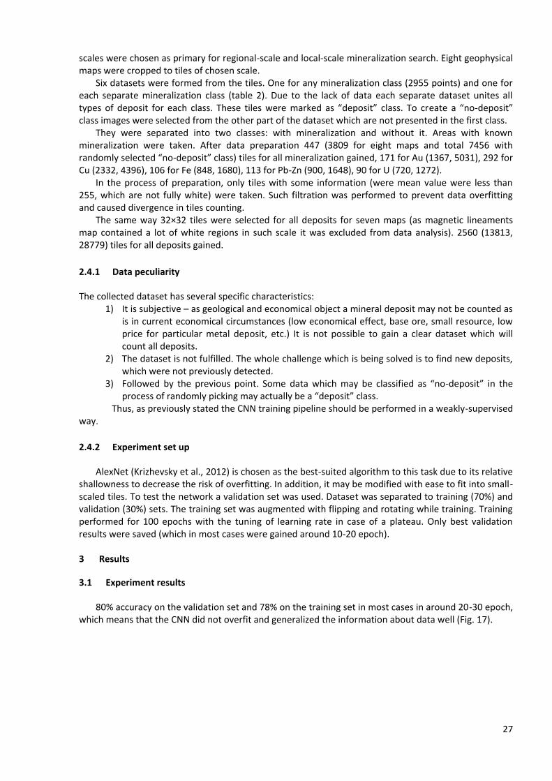
80% accuracy on the validation set and 78% on the training set in most cases in around 20-30 epoch, which means that the CNN did not overfit and generalized the information about data well (Fig. 17).

28

Fig. 17. Training plots examples for all deposits 256x256 titles (to the left), and for Cu deposits (on the right).

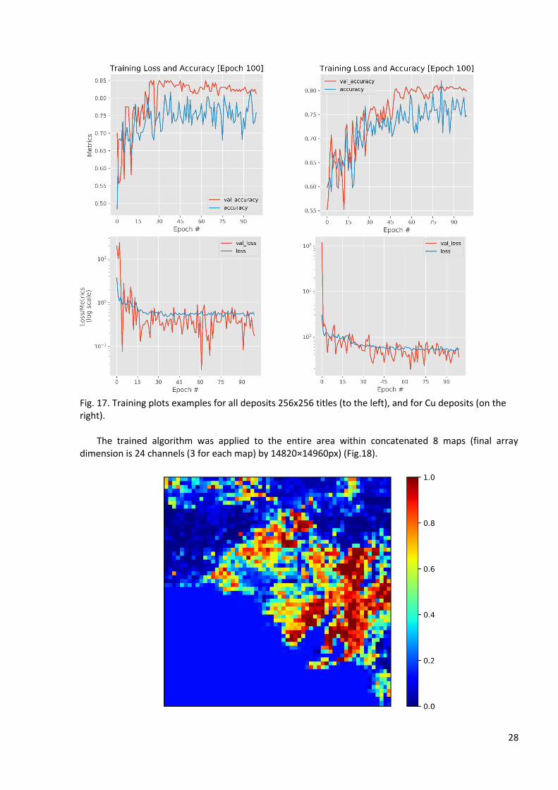
The trained algorithm was applied to the entire area within concatenated 8 maps (final array dimension is 24 channels (3 for each map) by 14820×14960px) (Fig.18).

29

Figure 18. CNN prediction results represented in a colormap. Each square represents the certainty of an algorithm in deposit allocation and can be used for further processing by a geologist. Legend to the colourmap is on the right.

As mentioned above we applied SoftMax operator to forecast certainty of an algorithm in the

prediction results which allow the geologist to use this information as a recommendation to further investigation of certain regions. Results presented on the fig. 18 are valuable for geologist as he may point his interest to certain regions. 3.2 Regional-scale forecast

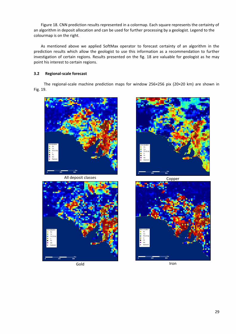
The regional-scale machine prediction maps for window 256×256 pix (20×20 km) are shown in Fig. 19.

All deposit classes

Copper

Gold

Iron

30

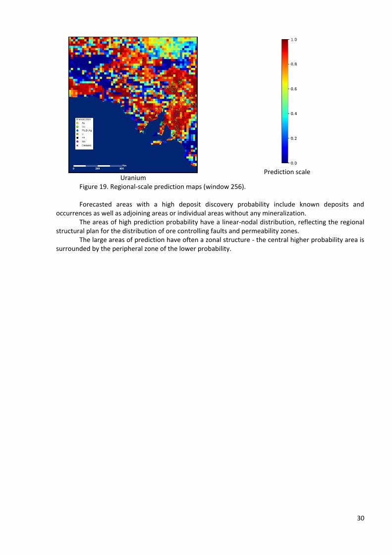
Uranium

Prediction scale

Figure 19. Regional-scale prediction maps (window 256). Forecasted areas with a high deposit discovery probability include known deposits and

occurrences as well as adjoining areas or individual areas without any mineralization. The areas of high prediction probability have a linear-nodal distribution, reflecting the regional

structural plan for the distribution of ore controlling faults and permeability zones. The large areas of prediction have often a zonal structure - the central higher probability area is

surrounded by the peripheral zone of the lower probability.

31

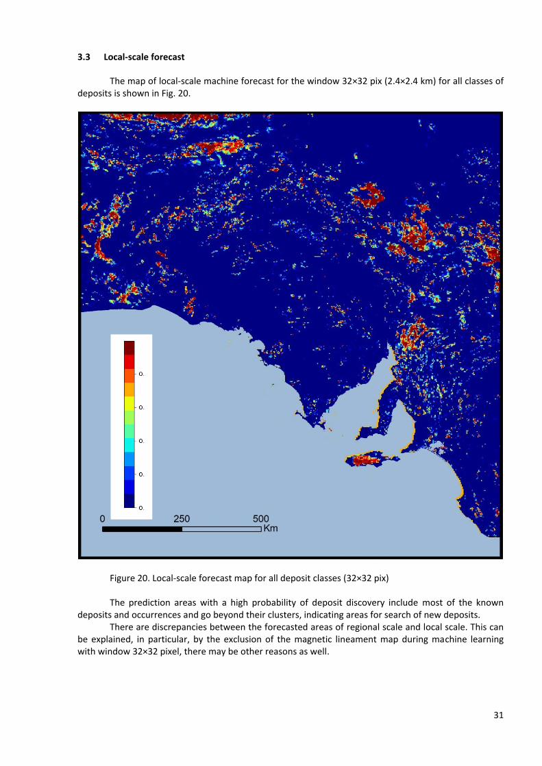
3.3 Local-scale forecast

The map of local-scale machine forecast for the window 32×32 pix (2.4×2.4 km) for all classes of deposits is shown in Fig. 20.

Figure 20. Local-scale forecast map for all deposit classes (32×32 pix) The prediction areas with a high probability of deposit discovery include most of the known

deposits and occurrences and go beyond their clusters, indicating areas for search of new deposits. There are discrepancies between the forecasted areas of regional scale and local scale. This can

be explained, in particular, by the exclusion of the magnetic lineament map during machine learning with window 32×32 pixel, there may be other reasons as well.

32

3.4 Comparison of the Machine Forecast results with the Geological Forecast results

Comparison of results of expert geological forecast and targeting and machine forecast was made for the Prominent Hill Cluster (Fig...) and for the Four Mile West Cluster.

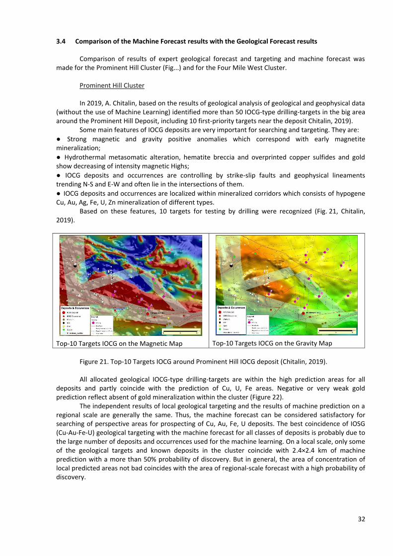
Prominent Hill Cluster In 2019, A. Chitalin, based on the results of geological analysis of geological and geophysical data

(without the use of Machine Learning) identified more than 50 IOCG-type drilling-targets in the big area around the Prominent Hill Deposit, including 10 first-priority targets near the deposit Chitalin, 2019).

Some main features of IOCG deposits are very important for searching and targeting. They are: ● Strong magnetic and gravity positive anomalies which correspond with early magnetite mineralization; ● Hydrothermal metasomatic alteration, hematite breccia and overprinted copper sulfides and gold show decreasing of intensity magnetic Highs; ● IOCG deposits and occurrences are controlling by strike-slip faults and geophysical lineaments trending N-S and E-W and often lie in the intersections of them. ● IOCG deposits and occurrences are localized within mineralized corridors which consists of hypogene Cu, Au, Ag, Fe, U, Zn mineralization of different types.

Based on these features, 10 targets for testing by drilling were recognized (Fig. 21, Chitalin, 2019).

Top-10 Targets IOCG on the Magnetic Map

Top-10 Targets IOCG on the Gravity Map

Figure 21. Top-10 Targets IOCG around Prominent Hill IOCG deposit (Chitalin, 2019). All allocated geological IOCG-type drilling-targets are within the high prediction areas for all

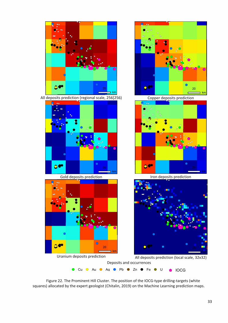
deposits and partly coincide with the prediction of Cu, U, Fe areas. Negative or very weak gold prediction reflect absent of gold mineralization within the cluster (Figure 22).

The independent results of local geological targeting and the results of machine prediction on a regional scale are generally the same. Thus, the machine forecast can be considered satisfactory for searching of perspective areas for prospecting of Cu, Au, Fe, U deposits. The best coincidence of IOSG (Cu-Au-Fe-U) geological targeting with the machine forecast for all classes of deposits is probably due to the large number of deposits and occurrences used for the machine learning. On a local scale, only some of the geological targets and known deposits in the cluster coincide with 2.4×2.4 km of machine prediction with a more than 50% probability of discovery. But in general, the area of concentration of local predicted areas not bad coincides with the area of regional-scale forecast with a high probability of discovery.

33

All deposits prediction (regional scale, 256[256)

Copper deposits prediction

Gold deposits prediction

Iron deposits prediction

Uranium deposits prediction

All deposits prediction (local scale, 32x32)


Figure 22. The Prominent Hill Cluster. The position of the IOCG-type drilling-targets (white

squares) allocated by the expert geologist (Chitalin, 2019) on the Machine Learning prediction maps.

!( Cu !( Au !( Ag !( Pb !( Zn !( Fe !( U $+ IOCG

34

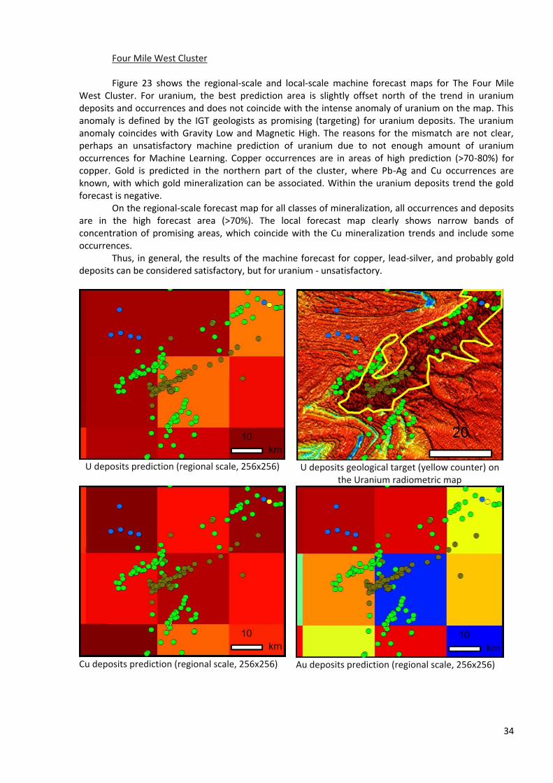
Four Mile West Cluster Figure 23 shows the regional-scale and local-scale machine forecast maps for The Four Mile

West Cluster. For uranium, the best prediction area is slightly offset north of the trend in uranium deposits and occurrences and does not coincide with the intense anomaly of uranium on the map. This anomaly is defined by the IGT geologists as promising (targeting) for uranium deposits. The uranium anomaly coincides with Gravity Low and Magnetic High. The reasons for the mismatch are not clear, perhaps an unsatisfactory machine prediction of uranium due to not enough amount of uranium occurrences for Machine Learning. Copper occurrences are in areas of high prediction (>70-80%) for copper. Gold is predicted in the northern part of the cluster, where Pb-Ag and Cu occurrences are known, with which gold mineralization can be associated. Within the uranium deposits trend the gold forecast is negative.

On the regional-scale forecast map for all classes of mineralization, all occurrences and deposits are in the high forecast area (>70%). The local forecast map clearly shows narrow bands of concentration of promising areas, which coincide with the Cu mineralization trends and include some occurrences.

Thus, in general, the results of the machine forecast for сopper, lead-silver, and probably gold deposits can be considered satisfactory, but for uranium - unsatisfactory.

U deposits prediction (regional scale, 256x256)

U deposits geological target (yellow counter) on

the Uranium radiometric map

Cu deposits prediction (regional scale, 256x256)

Au deposits prediction (regional scale, 256x256)

35

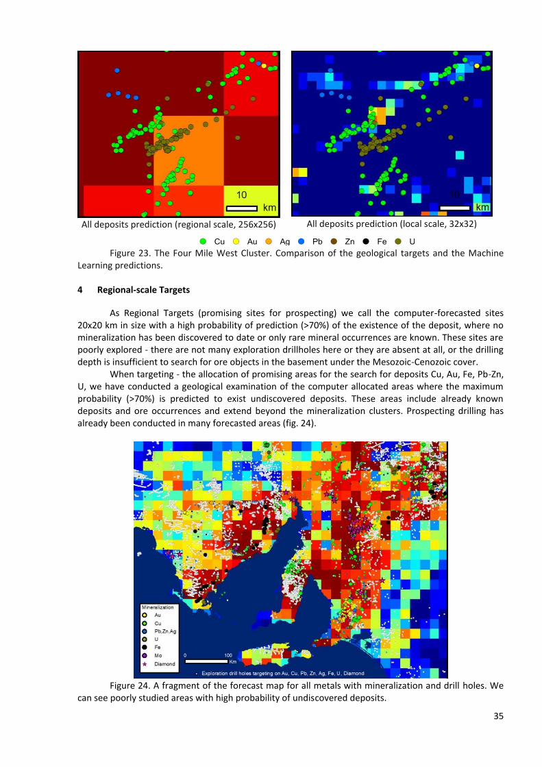
All deposits prediction (regional scale, 256x256)

All deposits prediction (local scale, 32x32)

Figure 23. The Four Mile West Cluster. Comparison of the geological targets and the Machine

Learning predictions.

4 Regional-scale Targets

As Regional Targets (promising sites for prospecting) we call the computer-forecasted sites 20х20 km in size with a high probability of prediction (>70%) of the existence of the deposit, where no mineralization has been discovered to date or only rare mineral occurrences are known. These sites are poorly explored - there are not many exploration drillholes here or they are absent at all, or the drilling depth is insufficient to search for ore objects in the basement under the Mesozoic-Cenozoic cover.

When targeting - the allocation of promising areas for the search for deposits Cu, Au, Fe, Pb-Zn, U, we have conducted a geological examination of the computer allocated areas where the maximum probability (>70%) is predicted to exist undiscovered deposits. These areas include already known deposits and ore occurrences and extend beyond the mineralization clusters. Prospecting drilling has already been conducted in many forecasted areas (fig. 24).

Figure 24. A fragment of the forecast map for all metals with mineralization and drill holes. We

can see poorly studied areas with high probability of undiscovered deposits.

!( Cu !( Au !( Ag !( Pb !( Zn !( Fe !( U

36

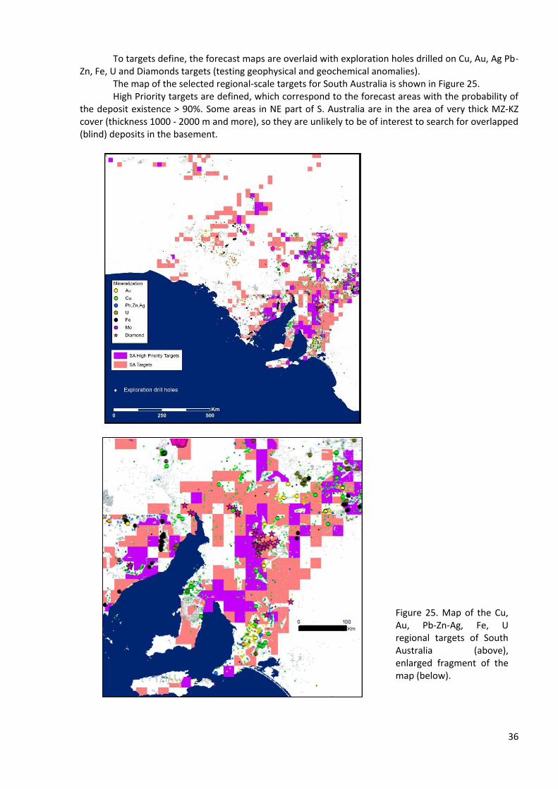
To targets define, the forecast maps are overlaid with exploration holes drilled on Cu, Au, Ag Pb-Zn, Fe, U and Diamonds targets (testing geophysical and geochemical anomalies).

The map of the selected regional-scale targets for South Australia is shown in Figure 25. High Priority targets are defined, which correspond to the forecast areas with the probability of

the deposit existence > 90%. Some areas in NE part of S. Australia are in the area of very thick MZ-KZ cover (thickness 1000 - 2000 m and more), so they are unlikely to be of interest to search for overlapped (blind) deposits in the basement.

Figure 25. Map of the Cu, Au, Pb-Zn-Ag, Fe, U regional targets of South Australia (above), enlarged fragment of the map (below).

37

5 Next steps

The proposed methods should be further investigated and modified to implement them as a system which can help a geologist to perform prospectivity mapping in several steps. First a large scale analysis performed. First, the areas are allocated in a regional scale. Regional high priority targets are detected and a geologist may choose which areas may be forecasted with a local machine learning algorithm in window 32x32 pix (2.4х2.4 km). Finally, he can perform more detailed geological analysis with a help of other algorithms (e.g. based on decision trees boosting, time-series analysis, etc.) of all

To develop a system for a local scale forecasting it is necessary to get much more high quality data on deposits and ore occurrences, including geological data for drill holes and trenches as well geochemical assay results. It is also necessary to use high-precision raster and vector maps on geology, geochemistry, and geophysics in a sequential manner with use of different scales up to ore body scale.

It is recommended to perform LESSA-lineament-analysis for local sites using space images and geophysical maps - to identify lineaments of different rank and to outline an areas and zones with different lineament density, these maps are also valuable for machine learning algorithms.

It is recommended to check the efficiency of use a high-resolution multispectral space images and ASTER images for areas where the Mesozoic-Cenozoic cover is absent.

We recommend to perform the geological analysis of local prospective areas in several steps: 1) identify ore control factors, 2) forecast perspective areas by an algorithm, 3) select the most prospective areas for complex prospecting works on the scale of 1:50 000 - 1:10 000, including deep drilling.

6 Conclusion

The proposed IGT method with use of machine learning algorithms to forecast mineral prospectivity by deposit made on the basis of preliminary geological analysis of all available data, selection of necessary useful maps and classification of deposits for the machine learning demonstrates high efficiency of the forecast (probability of deposit existence >70%) for the Cu, Au, Fe, Pb-Zn-Ag deposits in the regional scale and, in some cases, in the local scale.

The reliability of the machine forecast is proved by the coincidence of the selected areas of the high forecast probability with the perspective areas identified independently by an experienced geologist on geological and geophysical data without use of machine learning.

The best results are obtained by machine learning for all hypogene mineral deposits classes with the maximum population. The validity of such general population does not contradict the complex polychronous nature of mineralization in most deposits and occurrences. Population volume for each deposit classes is different. The most representative populations are for copper and gold. The least representative populations are for iron, uranium and base metals, so, the poor results of forecasts for these metals can be explained by the small population size.

The linear-nodal distribution of the selected forecast areas with a high probability of deposit discovery reflects, probably, the position of ore control regional faults and their intersection nodes.

It is recommended to make a local deposit forecast based on the analysis of detailed geological, geochemical and geophysical data and using Machine Learning. For machine learning and prediction on a local scale it is necessary to use much more data on deposits and ore occurrences, including geological logging data of drill holes and trenches and geochemical assay results. It is also necessary to use raster and vector maps on geology, geochemistry and geophysics in the deposit-ore-field-scale.

It will be useful to perform LESSA-lineament-analysis for local sites using space images and geophysical maps - to identify lineaments of different rank and to outline areas and zones with different lineament density, these maps can also be used for machine learning

For areas where the Mesozoic-Cenozoic cover absent, it is recommended to check the efficiency of use high-resolution multispectral space images and ASTER images for machine learning.

38

7 References

Apukhtina, O., Kamenetsky, V., Ehrig, K., Kamenetsky, M., Maas, R., Thompson, J., McPhie, J.,

Ciobanu, C., and Cook, N. (2017). Early, deep magnetite-fluorapatite mineralization at the Olympic Dam Cu-U-Au-Ag deposit, South Australia: Economic Geology, v. 112, pp. 1531–1542.

Belperio A. P. and Freeman H. Common Geological Characteristics of Prominent Hill and Olympic

Dam: Implications for Iron Oxide Copper-Gold Exploration Models. PACRIM 2004 Congress. The Australian Institute of Mining and Metallurgy Publications Series № 5/2004, pp. 115-125.

Ben Cave. (2010). "Copper - Gold exploration in the Middleback Ranges; source(s) of fluids and

metals". 2010. Thesis for: B.Sc. (Hons) University of Adelaide Advisor: Andreas Schmidt Mumm. Pp.177.

Brown, W.M., Gedeon, T.D., Groves, D.I., Barnes, R.G. (2000). Artificial neural networks: A new method for mineral prospectivity mapping. Aust. J. Earth Sci. 47, 757–770. https://doi.org/10.1046/j.1440-0952.2000.00807.x

Chitalin, A. F. (2019). Prediction IOCG deposits at Mount Woods. Explorer Challenge, 28 Feb - 31 May 2019; https://unearthed.solutions/u/submissions/prediction-iosg-deposits-mount-woods/ Andrey Chitalin_Proposal.pdf.

Devine, F. (2012). Porphyry Integration Project: Bringing Together Geoscience and Exploration Datasets for British Columbia' s Porphyry Districts. Technical report, Geoscience BC.

Eck, M., and Hodgkison, J. (2011). OZ MINERALS ANALYST VISIT PRESENTATION PART 1 – EXPLORATION OVERVIEW 18 April 2011 http://ozminerals.com

Ehrig, K., McPhie, J., and Kamenetsky, V. (2012). Geology and Mineralogical Zonation of the Olympic Dam Iron Oxide Cu-U-Au-Ag Deposit, South Australia: Society of Economic Geologists, Inc. Special Publication 16, pp. 237–267.

Goodfellow, I., Bengio, Y., Courville, A. (2016). Deep Learning. MIT Press. Granek, J. (2016). Application of Machine Learning Algorithms to Mineral Prospectivity Mapping.

University of British Columbia. https://doi.org/10.14288/1.0340340 Krizhevsky, A., Sutskever, I., Hinton, G.E. (2012). ImageNet Classification with Deep

Convolutional Neural Networks Alex. Adv. Neural Inf. Process. Syst. 25 2012. LeCun, Y., Boser, B., Denker, J.S., Henderson, D., Howard, R.E., Hubbard, W., Jackel, L.D. (1989).

Backpropagation Applied to Handwritten Zip Code Recognition. Neural Comput. 1, 541–551. https://doi.org/10.1162/neco.1989.1.4.541

Rundquist, D., Toulhoat, P., Cherkasov, S., Mercury, L., Guillaneau, J.-C., Sizaret, S., Robida, F.,

Cassard, D., Azaroual, M., Bertrand, G., Tourlière, B., Gumiaux, C., Hervio, N., Koshel, O., Sterligov, B. (Eds.) (2017). MINERAL PROSPECTIVITY CONFERENCE, MINERAL PROSPECTIVITY CONFERENCE.

Schlegel, T., Wagner, T., Wälle, M., and Heinrich, C. (2018). Hematite Breccia-Hosted Iron Oxide

Copper-Gold Deposits Require Magmatic Fluid Components Exposed to Atmospheric Oxidation: Evidence from Prominent Hill, Gawler Craton, South Australia: Economic Geology, v. 113, no. 3, pp. 597–644.

39

Schlegel, T., and Heinrich C. (2015). Lithology and Hydrothermal Alteration Control the Distribution of Copper Grade in the Prominent Hill Iron Oxide-Copper-Gold Deposit (Gawler Craton, South Australia): Economic Geology, v. 110, pp. 1953–1994.

Schlegel, T., Wagner, T., Boyce, A., and Heinrich, C. (2015). The Prominent Hill IOCG deposit in

South Australia - a deposit formation model based on geology, geochemistry, sulfur isotopes and fluid inclusions: Poster, Fluids and Mineral Deposits Group, ETH Zurich, Switzerland.

Ulyanov, D., Vedaldi, A., Lempitsky, V. (2020). Deep Image Prior. Int. J. Comput. Vis. 128, 1867–

1888. https://doi.org/10.1007/s11263-020-01303-4 Zlatopolsky, A.A. (1992). Program LESSA (Lineament Extraction and Stripe Statistical Analysis)

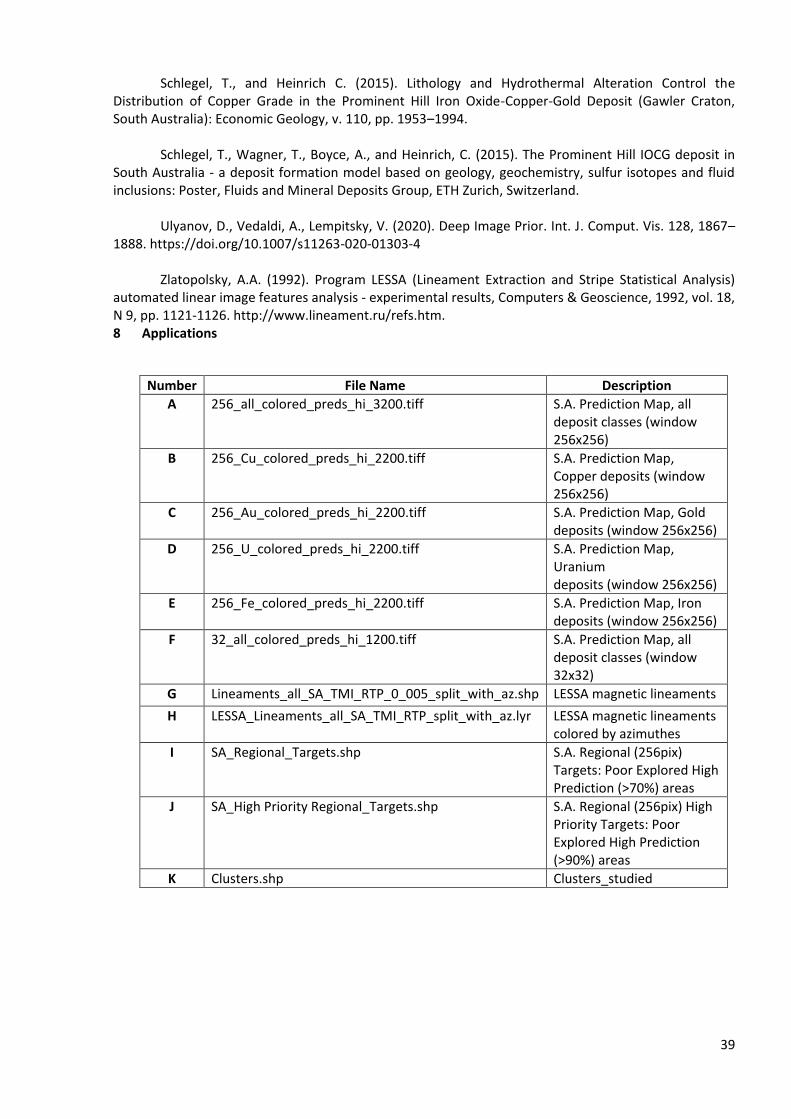
automated linear image features analysis - experimental results, Computers & Geoscience, 1992, vol. 18, N 9, pp. 1121-1126. http://www.lineament.ru/refs.htm. 8 Applications

Number File Name Description

A 256_all_colored_preds_hi_3200.tiff

S.A. Prediction Map, all deposit classes (window 256x256)

B 256_Cu_colored_preds_hi_2200.tiff

S.A. Prediction Map, Copper deposits (window 256x256)

C 256_Au_colored_preds_hi_2200.tiff

S.A. Prediction Map, Gold deposits (window 256x256)

D 256_U_colored_preds_hi_2200.tiff

S.A. Prediction Map, Uranium deposits (window 256x256)

E 256_Fe_colored_preds_hi_2200.tiff

S.A. Prediction Map, Iron deposits (window 256x256)

F 32_all_colored_preds_hi_1200.tiff S.A. Prediction Map, all deposit classes (window 32x32)

G Lineaments_all_SA_TMI_RTP_0_005_split_with_az.shp LESSA magnetic lineaments H LESSA_Lineaments_all_SA_TMI_RTP_split_with_az.lyr LESSA magnetic lineaments

colored by azimuthes I SA_Regional_Targets.shp S.A. Regional (256pix)

Targets: Poor Explored High Prediction (>70%) areas

J SA_High Priority Regional_Targets.shp S.A. Regional (256pix) High Priority Targets: Poor Explored High Prediction (>90%) areas

K Clusters.shp Clusters_studied

Documents

Geological A nalysis and Machine Learning for deposits