Embed Size (px)
Citation preview
Boletíndel Instituto de
Fisiografía y Geología
GEOID UNDULATIONS CHART OF THE SAN LUIS RANGE (ARGENTINA). GEOPHYSICAL APPLICATION
Laura L. CORNAGLIA & Antonio INTROCASO
Boletín del Instituto de Fisiografía y Geología 78(1-2), 2008.
Cornaglia L.L. & Introcaso A., 2008. Geoid undulations chart of the San Luis range (Argentina). Geophysical application. Boletín del Instituto de Fisiografía y Geología 78(1-2): 13-22. Rosario, 02-12-2008. ISSN 1666-115X.
Abstract.- In this work we show that it is possible to define the isostatic state of a geological structure using a geoid undulations chart. We have built: (1) a detailed geoid undulations chart of the San Luis range area using (a) the global geopotential model EIGEN CG03C for long wavelength free-air gravity anomalies and geoid undulations, and (b) observed residual free-air gravity anomalies and the equivalent sources method for short wavelength geoid undulations, and (2) a theoretical undulations chart of San Luis range area, involving effects from an isostatically compensated model. By comparing charts (1) and (2) we have found agreement between them, thus indicating the San Luis range is rather well isostatically balanced.
Key-words: Geological structure; Geoid; Isostasy.
Resumen.- Carta de ondulaciones del geoide de la Sierra de San Luis (Argentina). Aplicación geofísica. Nuestro propósito es demostrar que desde una carta de ondulaciones del geoide de buena resolución es posible inferir las características corticales de una estructura geológica. Para ello construimos: (1) una carta de ondulaciones del geoide sobre la sierra de San Luis con adecuado detalle empleando (a) anomalías de aire libre y ondulaciones del geoide de largas longitudes de onda provenientes del modelo global geopotencial EIGEN CG03C y (b) anomalías de aire libre residuales observadas y el método de fuentes equivalentes para calcular las ondulaciones del geoide de cortas longitudes de onda, y (2) una carta de ondulaciones del geoide que contiene los efectos isostáticos de un modelo perfectamente compensado. Comparando ambas cartas (1) y (2) encontramos una muy aceptable coincidencia entre ambas, indicando un buen balance isostático para la sierra de San Luis.
Palabras clave: Estructura geológica; Geoide; Isostasia.
Laura L.Cornaglia: Instituto Geofísico Sismológico Volponi (UNSJ), Meglioli 1160 (S), 5400 San Juan, Argentina, Grupo de Geofísica, IFIR (CONICET-UNR), Pellegrini 250, 2000 Rosario, Argentina.
Antonio Introcaso: Facultad de Ciencias Exactas, Ingeniería y Agrimensura (UNR), Grupo de Geofísica, IFIR (CONICET-UNR), Pellegrini 250, 2000 Rosario, Argentina.
Received: 01/08/2008; accepted: 15/11/2008.
13
Bol. Inst. Fis. Geol. 78: 13-22.Rosario - Argentina.
Copia Impresa / Printed Copy [€ 10+5]http://www.fceia.unr.edu.ar/fisiografia
INTRODUCTION The San Luis range is located NE of the homonymous Province, west-central Argentina. The range boundaries are: 32º00'- 33º30' S and 65º00'- 66º30' W. The range
2extends over 23000 km along an imaginary axis 150 km
long and NE strike. The range is 80 km wide. Altitudes are less than 2000 m. Three sedimentary basins are located arround the San Luis range: Las Salinas in the Northwest, Beazley in the South, Mercedes in the Southeast and Conlara Valley apart from the San Luis range of Comechingones range (Fig. 1).
Cornaglia & Introcaso (2004), working on a profile, have preliminarily pointed out a crustal thickness excess in the area; Crovetto & Introcaso (2004) have proposed short wavelength isostatic geoidic indicators to make a preliminary isostatic analysis of the San Luis range, concluding that geoid undulations allow validating classic gravimetry; Introcaso & Crovetto (2005) have presented different methods for building a geoid chart, in particular a chart for the San Luis range. All previous works on the San Luis range have presented preliminary conclusions because of the lack of consistent geoid undulations charts.
In this work we present a high resolution geoid undulations chart built using an equivalent sources method and observed free-air gravity anomalies (Fig. 2), practically Faye anomalies in view of the maturity of the topography. We have first obtained long wavelength geoid undulations (N ) using adequate cuts in the LWL
spherical harmonic expansions. We have used the global geopotential models EGM96 (Lemoine et al. 1998) and EIGEN GL03C (Förste et al. 2005). Then, from residual free-air gravity anomalies and equivalent sources
14 Cornaglia & Introcaso - Geoid undulations of the San Luis Range (Argentina)
methods, we have obtained short wavelength geoid undulations N . Total geoid undulations are: N = N + SWL T LWL
N . This expression was adjusted in eleven geoid height SWL
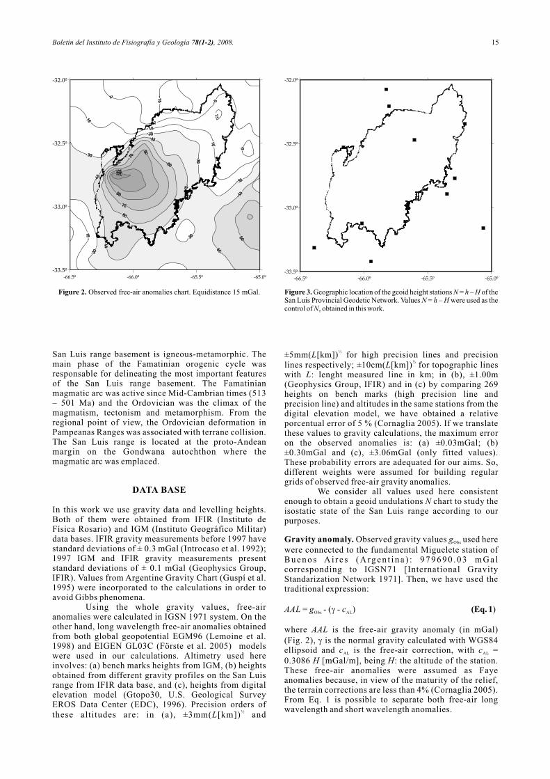
stations N = h – H (see Fig. 3). Finally, from San Luis range topographic altitudes, we have built an isostatically balanced model defined using T (standard N
crustal thickness): 33 km and R (crustal root bellow T ) = N
6.675 H , being H the topographic altitude. From direct T T
calculat ion and using r ight and homogeneous parallelepipeds we have obtained theoretical residual free-air gravity anomalies corresponding to the isostatically compensated model. Then, using the equivalent sources method, we have obtained the disturbing potential T and the isostatic geoid undulations N . Total isostatic geoid undulations are N = N + iSWL iT LWL
N . By comparing N and N we have found that the San iSWL T iT
Luis range is isostatically rather well balanced.
BRIEF DESCRIPTION OF THE SAN LUIS RANGE
Jordan & Allmendinger (1986) have pointed out that the Pampeanas Ranges geological province of Argentina is a region of large mountains. It is located on the western side of the thin skinned thrust belt of the Andean Mountains, coincident with a region where the subducted Nazca plate is sub-horizontal. Mountain ranges have been uplifted by reverse faulting and local folding. There are evidences of compressional earthquakes. The nearest shortening is estimated to be about 2%. Many of the faults are listric in the subsurface and flatten at mid to lower crustal depths. In opinion of Sato et al. (2003), the
B
Figure 1. A: Geographic location of the San Luis range. B: Location of the sedimentary basins nearby the San Luis range (Modified from Criado-Roqué et al. 1981).
A
15Boletín del Instituto de Fisiografía y Geología 78(1-2), 2008.
Figure 3. Geographic location of the geoid height stations N = h – H of the San Luis Provincial Geodetic Network. Values N = h – H were used as the control of N obtained in this work.T
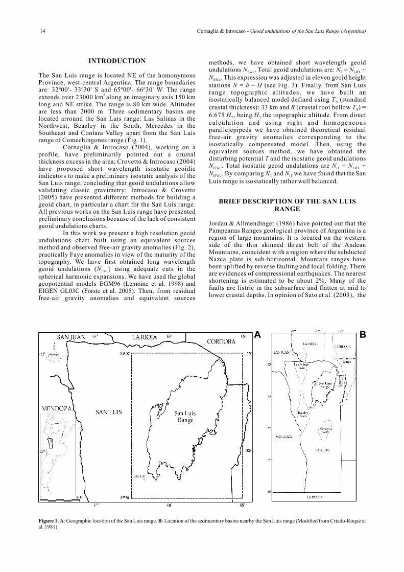
Figure 2. Observed free-air anomalies chart. Equidistance 15 mGal.
San Luis range basement is igneous-metamorphic. The main phase of the Famatinian orogenic cycle was responsable for delineating the most important features of the San Luis range basement. The Famatinian magmatic arc was active since Mid-Cambrian times (513 – 501 Ma) and the Ordovician was the climax of the magmatism, tectonism and metamorphism. From the regional point of view, the Ordovician deformation in Pampeanas Ranges was associated with terrane collision. The San Luis range is located at the proto-Andean margin on the Gondwana autochthon where the magmatic arc was emplaced.
DATA BASE
In this work we use gravity data and levelling heights. Both of them were obtained from IFIR (Instituto de Física Rosario) and IGM (Instituto Geográfico Militar) data bases. IFIR gravity measurements before 1997 have standard deviations of ± 0.3 mGal (Introcaso et al. 1992); 1997 IGM and IFIR gravity measurements present standard deviations of ± 0.1 mGal (Geophysics Group, IFIR). Values from Argentine Gravity Chart (Guspí et al. 1995) were incorporated to the calculations in order to avoid Gibbs phenomena.
Using the whole gravity values, free-air anomalies were calculated in IGSN 1971 system. On the other hand, long wavelength free-air anomalies obtained from both global geopotential EGM96 (Lemoine et al. 1998) and EIGEN GL03C (Förste et al. 2005) models were used in our calculations. Altimetry used here involves: (a) bench marks heights from IGM, (b) heights obtained from different gravity profiles on San Luis range from IFIR data base, and (c) heights from digital elevation model (Gtopo30, U.S. Geological Survey EROS Data Center (EDC), 1996). Precision orders of
½these altitudes are: in (a), 3mm(L[km]) and
the ,
±
±±
±
±± ±
½5mm(L[km]) for high precision lines and precision ½lines respectively; 10cm(L[km]) for topographic lines
with L: lenght measured line in km; in (b), 1.00m (Geophysics Group, IFIR) and in (c) by comparing 269 heights on bench marks (high precision line and precision line) and altitudes in the same stations from the digital elevation model, we have obtained a relative porcentual error of 5 % (Cornaglia 2005). If we translate these values to gravity calculations, the maximum error on the observed anomalies is: (a) 0.03mGal; (b)
0.30mGal and (c), 3.06mGal (only fitted values). These probability errors are adequated for our aims. So, different weights were assumed for building regular grids of observed free-air gravity anomalies.
We consider all values used here consistent enough to obtain a geoid undulations N chart to study the isostatic state of the San Luis range according to our purposes.
Gravity anomaly. Observed gravity values g used here Obs
were connected to the fundamental Miguelete station of B u e n o s A i r e s ( A rg e n t i n a ) : 9 7 9 6 9 0 . 0 3 m G a l corresponding to IGSN71 [International Gravity Standarization Network 1971]. Then, we have used the traditional expression:
AAL = g - (g - c ) Obs AL
where AAL is the free-air gravity anomaly (in mGal) (Fig. 2), g is the normal gravity calculated with WGS84 ellipsoid and c is the free-air correction, with c = AL AL
0.3086 H [mGal/m], being H: the altitude of the station. These free-air anomalies were assumed as Faye anomalies because, in view of the maturity of the relief, the terrain corrections are less than 4% (Cornaglia 2005). From Eq. 1 is possible to separate both free-air long wavelength and short wavelength anomalies.
(Eq. 1)
-66.5º -66.0º -65.5º -65.0º-33.5º
-33.0º
-32.5º
-32.0º
-66.5º -66.0º -65.5º -65.0º
-33.5º
-33.0º
-32.5º
-32.0º
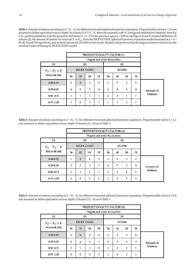
Table 1. Amount of stations according to E = N - N for different truncated spherical harmonic expansions. Proportionality factor k = 1.4 was T C
assumed to define equivalent sources depth. In column (1) E= N - N intervals assumed, with N : total geoid undulations obtained from Eq. T C T
3, N : geoid undulations from the geometric definition N = h - H (order precision approx. ± 0.05 m, see Figure 3) and E: residual difference; in C C
column (2), the amount of stations for intervals E vs N from the EIGEN CG03C spherical harmonic expansion model truncated at n = m = LWL
36, 40, 50 and 70 respectively, and on third column (3), EGM96 model results. Shaded cells point out that the largest amount of stations for the smallest E interval belongs to EIGEN CG03C model.
Table 2. Amount of stations according to E = N - N for different truncated spherical harmonic expansions. Proportionality factor k = 2.1 T C
was assumed to define equivalent sources depth. Columns (1) - (3) as in Table 1.
Table 3. Amount of stations according to E = N - N for different truncated spherical harmonic expansions. Proportionality factor k = 2.8 T C
was assumed to define equivalent sources depth. Columns (1) - (3) as in Table 1.
16 Cornaglia & Introcaso - Geoid undulations of the San Luis Range (Argentina)
GEOID UNDULATIONS CHART OF THE SAN LUIS RANGE
Although the well known ambigüity of potential field is a serious problem to obtain a consistent gravity model by inversion, it can be put into advantage to calculate geoid undulations (Introcaso 2004, 2006). From the equivalent sources method (fictitious, simple, rigurous), it is possible to define a model (ensemble of sources) that fits observed free-air anomalies removed from long wavelength effects. Then, from this fictitious model, we can directly calculate the disturbing potential (or anomalous potential) T, then obtain N from the formula
2of Bruns: N = T/g (see Torge 2001) with g = 9.80 m/s (Guspí et al. 2004, Introcaso & Crovetto 2005, Introcaso
2006). We have followed Guspí et al. (2004) who solved a linear equations system:
(Eq. 2)
for obtaining the intensities of equivalent sources c . G is j-8 3 -1 -2the gravitational constant 6.67x10 cm g s , T is the ji
disturbing potential at i station and l is the distance from ji
the station i to the source c . In order to calculate different j
long wavelength geoid undulations, the following expression was assumed:
N = N + N T LWL SWL (Eq. 3)
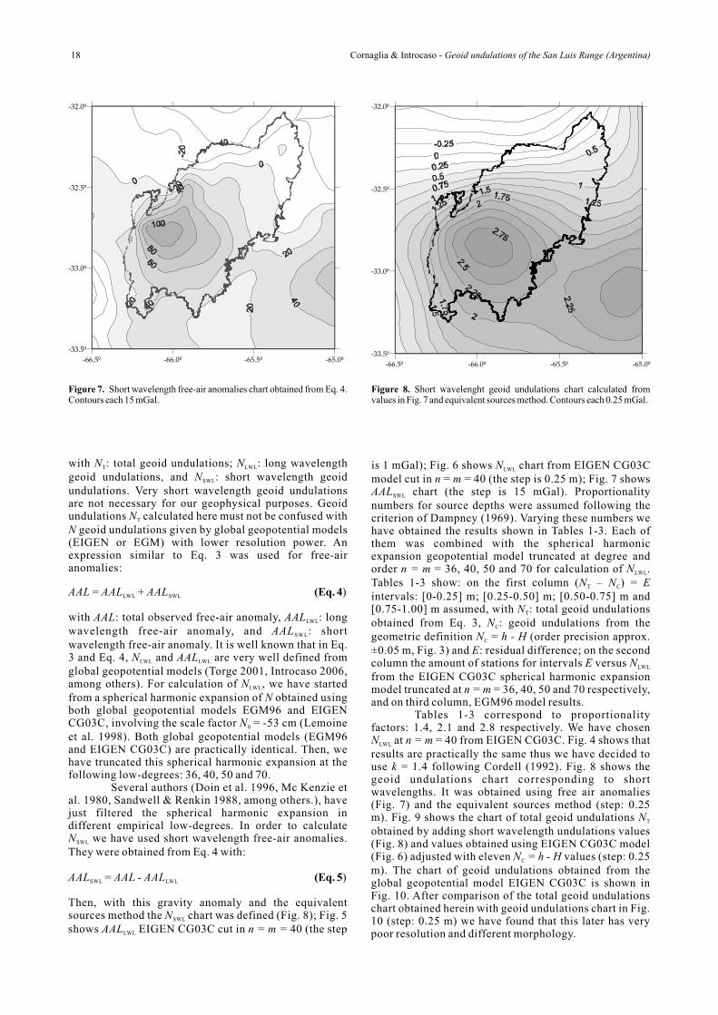
17Boletín del Instituto de Fisiografía y Geología 78(1-2), 2008.
Figure 6. Geoid undulations N chart from EIGEN CG03C model LWL
developed up to n = m = 40. Contours each 0.25 m.Figure 5. Free-air gravity anomalies AAL chart from EIGEN CG03C LWL
model developed up to n = m = 40. Contours each 1 mGal.
-66.5º -66.0º -65.5º -65.0º
-33.5º
-33.0º
-32.5º
-32.0º
-66.5º -66.0º -65.5º -65.0º
-33.5º
-33.0º
-32.5º
-32.0º
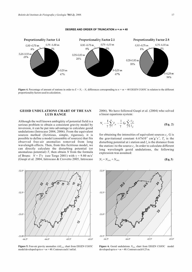
Figure 4. Percentage of amount of stations in order to E = N – N differences corresponding to n = m = 40 EIGEN CG03C in relation to the different T C
proportionality factors used in calculation.
DEGREE AND ORDER OF TRUNCATION n = m = 40
with N : total geoid undulations; N : long wavelength T LWL
geoid undulations, and N : short wavelength geoid SWL
undulations. Very short wavelength geoid undulations are not necessary for our geophysical purposes. Geoid undulations N calculated here must not be confused with T
N geoid undulations given by global geopotential models (EIGEN or EGM) with lower resolution power. An expression similar to Eq. 3 was used for free-air anomalies:
AAL = AAL + AALLWL SWL
with AAL: total observed free-air anomaly, AAL : long LWL
wavelength free-air anomaly, and AAL : short SWL
wavelength free-air anomaly. It is well known that in Eq. 3 and Eq. 4, N and AAL are very well defined from LWL LWL
global geopotential models (Torge 2001, Introcaso 2006, among others). For calculation of N , we have started LWL
from a spherical harmonic expansion of N obtained using both global geopotential models EGM96 and EIGEN CG03C, involving the scale factor N = -53 cm (Lemoine 0
et al. 1998). Both global geopotential models (EGM96 and EIGEN CG03C) are practically identical. Then, we have truncated this spherical harmonic expansion at the following low-degrees: 36, 40, 50 and 70.
Several authors (Doin et al. 1996, Mc Kenzie et al. 1980, Sandwell & Renkin 1988, among others.), have just filtered the spherical harmonic expansion in different empirical low-degrees. In order to calculate N we have used short wavelength free-air anomalies. SWL
They were obtained from Eq. 4 with:
AAL = AAL - AAL (Eq. 5)SWL LWL
Then, with this gravity anomaly and the equivalent sources method the N chart was defined (Fig. 8); Fig. 5 SWL
shows AAL EIGEN CG03C cut in n = m = 40 (the step LWL
(Eq. 4)
is 1 mGal); Fig. 6 shows N chart from EIGEN CG03C LWL
model cut in n = m = 40 (the step is 0.25 m); Fig. 7 shows AAL chart (the step is 15 mGal). Proportionality SWL
numbers for source depths were assumed following the criterion of Dampney (1969). Varying these numbers we have obtained the results shown in Tables 1-3. Each of them was combined with the spherical harmonic expansion geopotential model truncated at degree and order n = m = 36, 40, 50 and 70 for calculation of N . LWL
Tables 1-3 show: on the first column (N – N ) = E T C
intervals: [0-0.25] m; [0.25-0.50] m; [0.50-0.75] m and [0.75-1.00] m assumed, with N : total geoid undulations T
obtained from Eq. 3, N : geoid undulations from the C
geometric definition N = h - H (order precision approx. C
±0.05 m, Fig. 3) and E: residual difference; on the second column the amount of stations for intervals E versus N LWL
from the EIGEN CG03C spherical harmonic expansion model truncated at n = m = 36, 40, 50 and 70 respectively, and on third column, EGM96 model results.
Tables 1-3 correspond to proportionality factors: 1.4, 2.1 and 2.8 respectively. We have chosen N at n = m = 40 from EIGEN CG03C. Fig. 4 shows that LWL
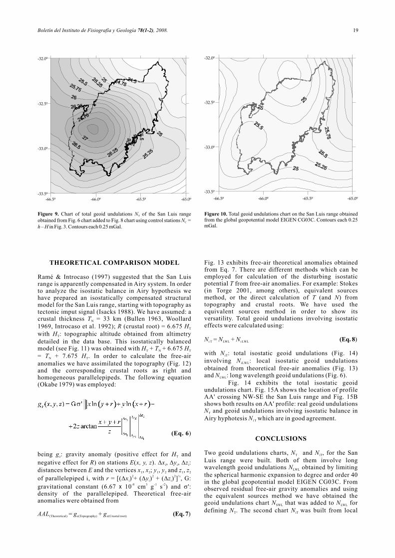
results are practically the same thus we have decided to use k = 1.4 following Cordell (1992). Fig. 8 shows the geoid undulations chart corresponding to short wavelengths. It was obtained using free air anomalies (Fig. 7) and the equivalent sources method (step: 0.25 m). Fig. 9 shows the chart of total geoid undulations N T
obtained by adding short wavelength undulations values (Fig. 8) and values obtained using EIGEN CG03C model (Fig. 6) adjusted with eleven N = h - H values (step: 0.25 C
m). The chart of geoid undulations obtained from the global geopotential model EIGEN CG03C is shown in Fig. 10. After comparison of the total geoid undulations chart obtained herein with geoid undulations chart in Fig. 10 (step: 0.25 m) we have found that this later has very poor resolution and different morphology.
18 Cornaglia & Introcaso - Geoid undulations of the San Luis Range (Argentina)
Figure 7. Short wavelength free-air anomalies chart obtained from Eq. 4. Contours each 15 mGal.
-66.5º -66.0º -65.5º -65.0º
-33.5º
-33.0º
-32.5º
-32.0º
Figure 8. Short wavelenght geoid undulations chart calculated from values in Fig. 7 and equivalent sources method. Contours each 0.25 mGal.
-66.5º -66.0º -65.5º -65.0º
-33.5º
-33.0º
-32.5º
-32.0º
THEORETICAL COMPARISON MODEL
Ramé & Introcaso (1997) suggested that the San Luis range is apparently compensated in Airy system. In order to analyze the isostatic balance in Airy hypothesis we have prepared an isostatically compensated structural model for the San Luis range, starting with topography as tectonic imput signal (Isacks 1988). We have assumed: a crustal thickness T = 33 km (Bullen 1963, Woollard N
1969, Introcaso et al. 1992); R (crustal root) = 6.675 H T
with H : topographic altitude obtained from altimetry T
detailed in the data base. This isostatically balanced model (see Fig. 11) was obtained with H + T + 6.675 H T N T
= T + 7.675 H . In order to calculate the free-air N T
anomalies we have assimilated the topography (Fig. 12) and the corresponding crustal roots as right and homogeneous parallelepipeds. The following equation (Okabe 1979) was employed:
(Eq. 6)
being g : gravity anomaly (positive effect for H and z T
negative effect for R) on stations E(x, y, z). Dx , Dy , Dz : i i i
distances between E and the vertices x , x ; y , y and z , z 1 2 1 2 1 22 2 2 ½of parallelepiped i, with r = [(Dx ) + (Dy ) + (Dz ) ] , G: i i i-8 3 -1 -2gravitational constant (6.67 x 10 cm g s ) and s':
density of the parallelepiped. Theoretical free-air anomalies were obtained from
AAL = g + g (Eq. 7)(Theoretical) z(Topography) z(Crustal root)
Fig. 13 exhibits free-air theoretical anomalies obtained from Eq. 7. There are different methods which can be employed for calculation of the disturbing isostatic potential T from free-air anomalies. For example: Stokes (in Torge 2001, among others), equivalent sources method, or the direct calculation of T (and N) from topography and crustal roots. We have used the equivalent sources method in order to show its versatility. Total geoid undulations involving isostatic effects were calculated using:
N = N + Ni T LWL i LWL
with N : total isostatic geoid undulations (Fig. 14) iT
involving N : local isostatic geoid undulations iLWL
obtained from theoretical free-air anomalies (Fig. 13) and N : long wavelength geoid undulations (Fig. 6).LWL
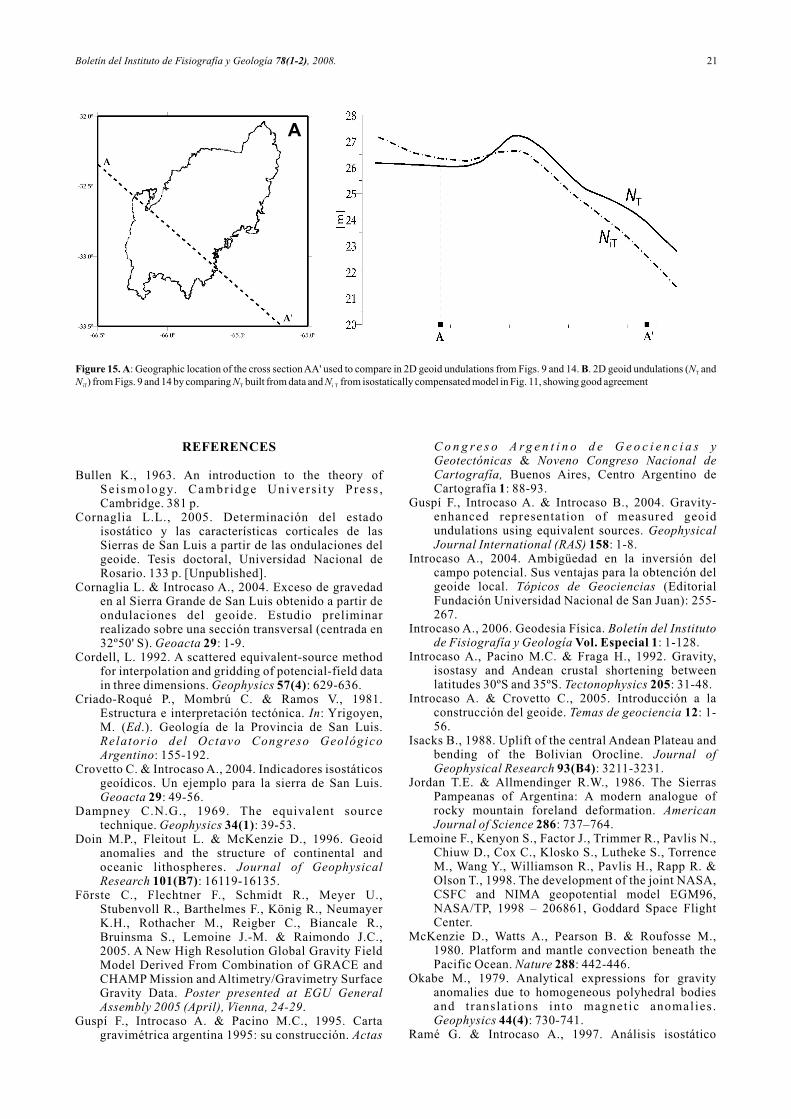
Fig. 14 exhibits the total isostatic geoid undulations chart. Fig. 15A shows the location of profile AA' crossing NW-SE the San Luis range and Fig. 15B shows both results on AA' profile: real geoid undulations N and geoid undulations involving isostatic balance in T
Airy hyphotesis N which are in good agreement.i T
CONCLUSIONS
Two geoid undulations charts, N and N , for the San T iT
Luis range were built. Both of them involve long wavelength geoid undulations N obtained by limiting LWL
the spherical harmonic expansion to degree and order 40 in the global geopotential model EIGEN CG03C. From observed residual free-air gravity anomalies and using the equivalent sources method we have obtained the geoid undulations chart N that was added to N for SWL LWL
defining N . The second chart N was built from local T iT
(Eq. 8)
19Boletín del Instituto de Fisiografía y Geología 78(1-2), 2008.
Figure 9. Chart of total geoid undulations N of the San Luis range T
obtained from Fig. 6 chart added to Fig. 8 chart using control stations N = C
h – H in Fig. 3. Contours each 0.25 mGal.
-66.5º -66.0º -65.5º -65.0º
-33.5º
-33.0º
-32.5º
-32.0º
Figure 10. Total geoid undulations chart on the San Luis range obtained from the global geopotential model EIGEN CG03C. Contours each 0.25 mGal.
-66.5º -66.0º -65.5º -65.0º
-33.5º
-33.0º
-32.5º
-32.0º
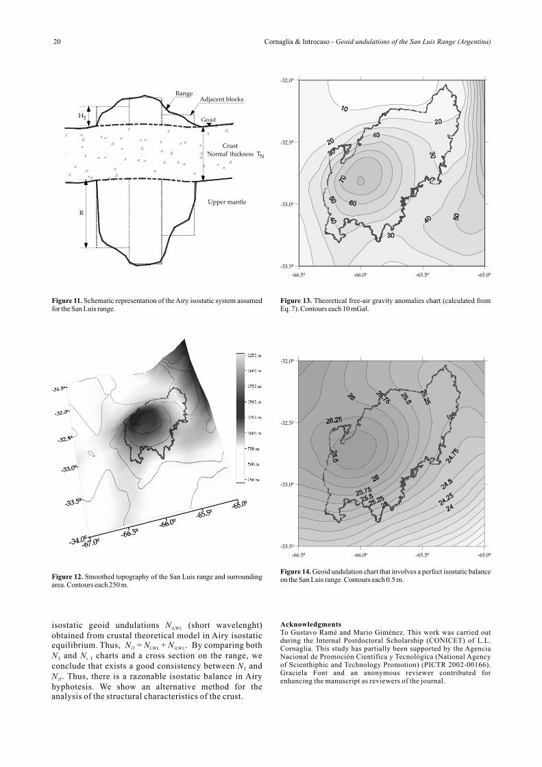
Figure 12. Smoothed topography of the San Luis range and surrounding area. Contours each 250 m.
isostatic geoid undulations N (short wavelenght) iLWL
obtained from crustal theoretical model in Airy isostatic equilibrium. Thus, N = N + N . By comparing both iT LWL iLWL
N and N charts and a cross section on the range, we T i T
conclude that exists a good consistency between N and T
N . Thus, there is a razonable isostatic balance in Airy iT
hyphotesis. We show an alternative method for the analysis of the structural characteristics of the crust.
AcknowledgmentsTo Gustavo Ramé and Mario Giménez. This work was carried out during the Internal Postdoctoral Scholarship (CONICET) of L.L. Cornaglia. This study has partially been supported by the Agencia Nacional de Promoción Científica y Tecnológica (National Agency of Scienthiphic and Technology Promotion) (PICTR 2002-00166). Graciela Font and an anonymous reviewer contributed for enhancing the manuscript as reviewers of the journal.
20 Cornaglia & Introcaso - Geoid undulations of the San Luis Range (Argentina)
-66.5º -66.0º -65.5º -65.0º
-33.5º
-33.0º
-32.5º
-32.0º
Figure 14. Geoid undulation chart that involves a perfect isostatic balance on the San Luis range. Contours each 0.5 m.
Figure 11. Schematic representation of the Airy isostatic system assumed for the San Luis range.
R
THGeoid
NT'Normal' thickness
RangeAdjacent blocks
Upper mantle
Crust
Figure 13. Theoretical free-air gravity anomalies chart (calculated from Eq. 7). Contours each 10 mGal.
-66.5º -66.0º -65.5º -65.0º
-33.5º
-33.0º
-32.5º
-32.0º
REFERENCES
Bullen K., 1963. An introduction to the theory of Se i smology. Cambr idge Univers i ty Press , Cambridge. 381 p.
Cornaglia L.L., 2005. Determinación del estado isostático y las características corticales de las Sierras de San Luis a partir de las ondulaciones del geoide. Tesis doctoral, Universidad Nacional de Rosario. 133 p. [Unpublished].
Cornaglia L. & Introcaso A., 2004. Exceso de gravedad en al Sierra Grande de San Luis obtenido a partir de ondulaciones del geoide. Estudio preliminar realizado sobre una sección transversal (centrada en 32º50' S). Geoacta 29: 1-9.
Cordell, L. 1992. A scattered equivalent-source method for interpolation and gridding of potencial-field data in three dimensions. Geophysics 57(4): 629-636.
Criado-Roqué P., Mombrú C. & Ramos V., 1981. Estructura e interpretación tectónica. In: Yrigoyen, M. (Ed.). Geología de la Provincia de San Luis. Relatorio del Octavo Congreso Geológico Argentino: 155-192.
Crovetto C. & Introcaso A., 2004. Indicadores isostáticos geoídicos. Un ejemplo para la sierra de San Luis. Geoacta 29: 49-56.
Dampney C.N.G., 1969. The equivalent source technique. Geophysics 34(1): 39-53.
Doin M.P., Fleitout L. & McKenzie D., 1996. Geoid anomalies and the structure of continental and oceanic lithospheres. Journal of Geophysical Research 101(B7): 16119-16135.
Förste C., Flechtner F., Schmidt R., Meyer U., Stubenvoll R., Barthelmes F., König R., Neumayer K.H., Rothacher M., Reigber C., Biancale R., Bruinsma S., Lemoine J.-M. & Raimondo J.C., 2005. A New High Resolution Global Gravity Field Model Derived From Combination of GRACE and CHAMP Mission and Altimetry/Gravimetry Surface Gravity Data. Poster presented at EGU General Assembly 2005 (April), Vienna, 24-29.
Guspí F., Introcaso A. & Pacino M.C., 1995. Carta gravimétrica argentina 1995: su construcción. Actas
C o n g r e s o A r g e n t i n o d e G e o c i e n c i a s y Geotectónicas & Noveno Congreso Nacional de Cartografía, Buenos Aires, Centro Argentino de Cartografía 1: 88-93.
Guspí F., Introcaso A. & Introcaso B., 2004. Gravity-enhanced representation of measured geoid undulations using equivalent sources. Geophysical Journal International (RAS) 158: 1-8.
Introcaso A., 2004. Ambigüedad en la inversión del campo potencial. Sus ventajas para la obtención del geoide local. Tópicos de Geociencias (Editorial Fundación Universidad Nacional de San Juan): 255-267.
Introcaso A., 2006. Geodesia Física. Boletín del Instituto de Fisiografía y Geología Vol. Especial 1: 1-128.
Introcaso A., Pacino M.C. & Fraga H., 1992. Gravity, isostasy and Andean crustal shortening between latitudes 30ºS and 35ºS. Tectonophysics 205: 31-48.
Introcaso A. & Crovetto C., 2005. Introducción a la construcción del geoide. Temas de geociencia 12: 1-56.
Isacks B., 1988. Uplift of the central Andean Plateau and bending of the Bolivian Orocline. Journal of Geophysical Research 93(B4): 3211-3231.
Jordan T.E. & Allmendinger R.W., 1986. The Sierras Pampeanas of Argentina: A modern analogue of rocky mountain foreland deformation. American Journal of Science 286: 737–764.
Lemoine F., Kenyon S., Factor J., Trimmer R., Pavlis N., Chiuw D., Cox C., Klosko S., Lutheke S., Torrence M., Wang Y., Williamson R., Pavlis H., Rapp R. & Olson T., 1998. The development of the joint NASA, CSFC and NIMA geopotential model EGM96, NASA/TP, 1998 – 206861, Goddard Space Flight Center.
McKenzie D., Watts A., Pearson B. & Roufosse M., 1980. Platform and mantle convection beneath the Pacific Ocean. Nature 288: 442-446.
Okabe M., 1979. Analytical expressions for gravity anomalies due to homogeneous polyhedral bodies and t ranslat ions into magnet ic anomalies . Geophysics 44(4): 730-741.
Ramé G. & Introcaso A., 1997. Análisis isostático
21Boletín del Instituto de Fisiografía y Geología 78(1-2), 2008.
A
Figure 15. A: Geographic location of the cross section AA' used to compare in 2D geoid undulations from Figs. 9 and 14. B. 2D geoid undulations (N and T
N ) from Figs. 9 and 14 by comparing N built from data and N from isostatically compensated model in Fig. 11, showing good agreement iT T i T
B
preliminar de la Sierra Grande de San Luis, Argentina. Revista de la Asociación Geológica Argentina 53(3): 379-386.
Sandwell D. & Renkin M.L., 1988. Compensation of swells and plateaus in the North Pacific. Journal of Geophysical Research 93(B4): 2775-2783.
Sato A.M., Gonzalez P.D. & Llambías E.J., 2003. Evolución del orógeno Famatiniano en la Sierra de San Luis: magmatismo de arco, deformación y metamorfismo de bajo a alto grado. Revista de la Asociación Geológica Argentina 58(4): 487-504.
rdTorge W., 2001. Geodesy (3 edition). Walter de Gruyter. Berlin-New York. 416 p.
Woollard G., 1969. Regional Variations in Gravity. Geophysical Monograph. American Geophysical Union 13: 320-341.
22 Cornaglia & Introcaso - Geoid undulations of the San Luis Range (Argentina)


![Untitled-1 [] · largas e irregulares, sobre fundo avermelhado As rajas tan. tas e largas entre elas, 0 trecho de fundo que aparece quag da mesma largura das Máscara preta. CABEÇA](https://img.pdfslide.us/doc/110x75/5f12106e15fabc63fe208a1f/untitled-1-largas-e-irregulares-sobre-fundo-avermelhado-as-rajas-tan-tas-e.jpg)