GEOGRAPHY AND AGRICULTURAL PRODUCTIVITY … · Why Study Geography and Agriculture? 2 Why Does this Analysis Focus on Foodgrains?4 Other Analysis of Agricultural Productivity in India6

GEOGRAPHY AND AGRICULTURAL PRODUCTIVITY IN INDIA: IMPLICATIONS FOR TAMIL NADU

Submitted to: State Government of Tamil Nadu

Prepared by: Rina Agarwala Rachel Gisselquist

Harvard Institute for International Development

With the Direction of Dr. Nirupam Bajpai, Director, HIID’s India Project, And Dr. Jeffrey D. Sachs, Director, HIID

April 6, 1999

i

TABLE OF CONTENTS

Pages

Table of Contents i

EXECUTIVE SUMMARY iii

I. Overview 1

Statement of Objectives 1

Why Study Geography and Agriculture? 2

Why Does this Analysis Focus on Foodgrains? 4

Other Analysis of Agricultural Productivity in India 6

Tamil Nadu is an Ideal Case Study 6

Overview of the paper 7

II. Methods and Tools 8

Step 1: Building the Data Set 8

Step 2: Identifying Patterns Using Geographic

Information Systems 10

Step 3: Designing an Empirical Model 10

III. Regional Foodgrain Trends 12

National Trends (1967-1980) 12

National Trends (1981-present) 13

A Closer Look at Foodgrain Yield Trends

in Tamil Nadu 14

IV. Geographic Variation and Foodgrain Yields 17

Variable 1: Koeppen Zones 17

Variable 2: Average Precipitation 19

Variable 3: Elevation 20

i i

Variable 4: Distance to the Nearest Navigable River 20

Variable 5: Soil Suitability Index 20

V. A Model of Geography and Foodgrain Yields 22

Model 1: Isolating the Effects of Koeppen

Zones on Yields 22

Model 2: Isolating the Effects of Rainfall

and Temperature Across Koeppen Zones 28

VI. Additional Differences A Cross Koeppen Zones 36

Comparison of Non-Geographic

Determinants Across Climate Zones 36

A Model of Fertilizer Use and Koeppen Zones 38

VII.Policy Recommendations 41

1. Include Geographic Factors in Economic

Analysis of Tamil Nadu’s Agriculture 41

2. Evaluate the Effects of Tamil Nadu’s

Agricultural Input Policies on Different

Agro-Climatic Production Environments

Across Districts 42

3. Encourage Research on New Technologies

Adapted to Tamil Nadu’s Geography 43

4. Support the Adoption of Technologies

Suited to Tamil Nadu’s Geography 45

5. Address Concerns of Agricultural Risk

Caused by Tamil Nadu’s Climate 46

6. Continue Investments in Tamil Nadu’s

Manufacturing and Trade Sectors 48

Pages

IV. Geographic Variation and Foodgrain Yields—cont.

iii

Pages

B I B L I O G R A P H Y 49

Appendices

Appendix A: Maps of Regional Foodgrain

and Input Trends

Appendix B: State Geography and

Foodgrain Yields

EXECUTIVE SUMMARY

The Problem: The growth rate of agriculture in Tamil Nadu

may be cause for concern. Recent studies by Professor

Jeffrey Sachs show that tropical conditions, such as Tamil Nadu’s

can slow economic growth through lower levels of agricultural

productivity. In 1995-96, the negative growth of Tamil Nadu’s

agricultural sector pulled the state’s growth rate down so low

that Tamil Nadu was unable to meet its growth target for the

Eighth Plan. Moreover, farmers in Tamil Nadu are shifting away

from foodgrain production to higher value commercial crops,

thereby raising substantial food security concerns. A continued

decline in Tamil Nadu’s agricultural sector, particularly in

foodgrains, could have grave implications for the State’s large

percentage of rural poor, food supplies and long term growth.

This Report: Since the Green Revolution began in the

late 1960s, India has experienced considerable regional varia-

tion in agricultural productivity. In particular, states in the

Northwest have consistently performed better than central and

southern states. Existing analysis on the determinants of this

variation have focussed on economic policies and institutions.

This report analysis the effects of geography on cross-state

variations in rice, wheat, maize and total foodgrain yield within

India and presents the policy implications of this analysis for

the State Government of Tamil Nadu. It uses the tools of sta-

tistical analysis, Geographic Information Systems, and econo-

metric models based on a production function approach. To

measure geographic variation, this study uses rainfall and tem-

perature data, as well as the “Koeppen Zone” measure, an

indicator of agro-climatic characteristics. The study is intended

to complement work done by other analysts on the effects of

economic policy on agriculture.

Findings: This analysis finds that the differences in foodgrainyields among states in northern, central, and southern India are

strongly linked to regional geographic variation. Geography has

2

an effect even when income, agricultural inputs, and fertilizer

are held constant. Specific findings are as follows:

* An empirical model shows that tropical zones, like Tamil

Nadu, have less positive effects on yields than dry

zones, like Punjab and Harayana. To isolate the

effects of Koeppen Zones on yields, the model holds

constant labor density, fertilizer lagged NSDP, and the

four primary Koeppen Zones represented in India. The

model explains over 99 per cent of the variation in

foodgrain yields across states in 1991.

* A Second empirical model illustrates that precipitation

and temperature patterns in tropical and dry states have

the largest impact on increasing foodgrain yields above

those in temperate states, like Uttar Pradesh and Madhya

Pradesh. The temperate Zone’s more volatile precipi-

tation levels help explain why its yields are lowest. To

isolate the effects of rainfall and temperature across

Koeppen Zones, this model uses more detailed infor-

mation from the World Bank covering the period 1967-86.

* Finally, this analysis shows that dry states have the

highest agricultural input levels. This suggests that tech-

nology and inputs may be one channel through which

geography affects agricultural productivity.

Recommendations: These findings raise important con-cerns for tropical states like Tamil Nadu. They suggest that

analysis of geography and agricultural productivity within India

can help Tamil Nadu improve its own agricultural investments

across geographically advantaged and disadvantaged districts.

It can also help Tamil Nadu better understand its position and

opportunities relative to other states in India. This report con-

cludes with the following six recommendations to assist the Tamil

Nadu Government to incorporate geographic analysis into its

agricultural policy:

1. Include geographic factors in economic analysis of Tamil Nadu’sagriculture. Within Tamil Nadu, the state government will gainvaluable insight into the causes of district level variations in yieldsby applying the methods described in this report. The Tamil NaduGovernment can also build on this report to increase understand-ing of its geographic advantages and disadvantages relative to otherstates.

3

2. Evaluate the effects of Tamil Nadu’s agricultural input policies ondifferent agro-climatic production environments across districts.This report shows that some agro-climatic environments are morefavourable for HYV and input use and thus have higher technologyand input levels. Tamil Nadu has attempted to raise input levelsthroughout the state through subsidies and infrastructure projects.In evaluating the effects of these policies, the state should measurewhether they are succeeding in both favourable and unfavourableproduction environments within the state.

3. Encourage research on new technology adopted to Tamil Nadu’sgeography. India has one of the world’s largest public agriculturalresearch systems. The North, however, enjoys the largest shareof research resources. The Tamil Nadu Government shouldpromote increased research focussing on the unique needs of theSouth’s geography through national public councils, stateagricultural Universities, the private sector, and internationalpartnerships.

4. Support the adoption of existing technologies suited toTamil Nadu’s geography. While Tamil Nadu cannot change itsgeographic profile, it can increase yields through the use of exist-ing technologies that are well-suited to its unique geography.Providing farmers with information on new technologies andreleasing new technologies to the market for purchase by farmerscan assist farmers in adopting technologies suited to Tamil Nadu’sgeography.

5. Address concerns of agricultural risk caused by Tamil Nadu’sclimate. This study illustrates that volatility in rainfall andtemperature plays an important role in agricultural yields.Uncertainty has led Tamil Nadu’s farmers to favour reduced risksover high yields, thereby slowing the growth of the state’sagricultural sector. The Tamil Nadu Government can reduce thecosts of uncertainty by providing farmers with information aboutweather and strengthening credit and insurance institutions withinthe state.

6. Continue investments in Tamil Nadu’s manufacturing and tradesectors. Some effects of geography on yields can be mitigatedby technology and inputs that are suited to regional geography.In the long run, however, Tamil Nadu may naturally shift awayfrom agriculture to other, more profitable sectors of the economy.Tamil Nadu appears to be making this transition, but should not

ignore agriculture in the process.

4

I. OVERVIEW

This policy analysis falls under the Harvard Institute for

International Developments’ three year contract with the State

Government of Tamil Nadu, India. Under this contract, HIID

provides Tamil Nadu with technical assistance and policy advice

to further the state’s macroeconomic growth. Research and

analysis were conducted under the guidance of Professor Jeffrey

Sachs, Director of HIID, and Dr. Nirupam Bajpai, Director of

HIID’s India Program.

STATEMENT OF OBJECTIVES

The primary objective of this policy analysis is to help the

Tamil Nadu Government increase its understanding of the

determinants of foodgrain productivity in India. Such

understanding can lead to more targeted agricultural

development strategies that promote growth, alleviate poverty,

and ensure food security for the state’s growing population.

Traditional studies have focussed on economic policies and

institutions as the primary determinants of Indian agricultural

productivity. This analysis looks at geography as another

potential determinant of agricultural productivity, with particular

focus on foodgrains, across Indian states. The analysis provides

the State Government with information to complement existing

studies. It highlights the implications geography may have on

Tamil Nadu’s foodgrain productivity relative to other states and

concludes with six policy recommendations to assist the State

Government to incorporate geographic analysis into

development polices.

This report uses statistical and econometric analysis and

Geographic Information Systems to study the impact of geog-

raphy on variations in foodgrain yield across India’s states. It

represents a first step in applying the methods of recent HIID

cross-country studies on geography and agricultural productivity

to state-level analysis of foodgrain productivity in India.

This analysis answers the following questions:

* What are the recent trends in rice, wheat, maize, andtotal foodgrain yields in India and in Tamil Nadu?

* How do state variations in foodgrain yields match upwith geographic variations?

5

* Holding income, agricultural inputs, and technologyconstant, does geographic variation have an impact on

foodgrain yields in India?

* Through what indirect channels might geography im-pact foodgrain yields in India?

* What are the policy implications of this analysis forTamil Nadu?

WHY STUDY GEOGRAPHY AND AGRICULTURE?

Recent cross-country analysis conducted by HIID haveshown, that, in addition to economic policy, geography hasimportant effects on cross-country variations in economic growth.

Jeffrey Sachs points out that agricultural productivity is one ofthe three channels through which geography affects economic

growth2. John Gallup’s paper “Agricultural Productivity andGeography” shows that agricultural output per person is muchlower in tropical than in temperate regions.3

These findings have important implications for development

in India. Twenty-five per cent of India’s gross domestic product(GDP) comes from agriculture, 75 per cent of the population

lives in rural areas, and 40 per cent of the land is in the tropics.While India’s location in the tropics suggests that it is at adisadvantage in terms of agricultural productivity, India cannot

ignore the agricultural sector. First, most of the country’s citizensstill live in rural areas and depend on agriculture for their

livelihood. In 1993, thirty-seven per cent of the rural population,totalling 268 million people, lived below the poverty line.Second, the country’s population of 961 million demands

enormous food supplies, which must grow at least as fast asprojected population growth rates.

Likewise, these findings have important implications for

Tamil Nadu for four reasons. First, 95 per cent of Tamil Nadu’sland is in the tropics. Second, Tamil Nadu’s foodgrainproduction is decreasing as farmers shift to higher value crops,

thereby raising food security concerns for the state.

1 The acronym “HIID” is used to refer to the Harvard Institute for International Development

throughout this report.

2 Gallup, John Luke and Jeffrey Sachs, “Geography and Economic Development”, Harvard

Institute for International Development (April 1998).

3 Gallup, John Luke, “Agriculture Productivity and Geography,” Harvard Institute forInternational Development (1998).

6

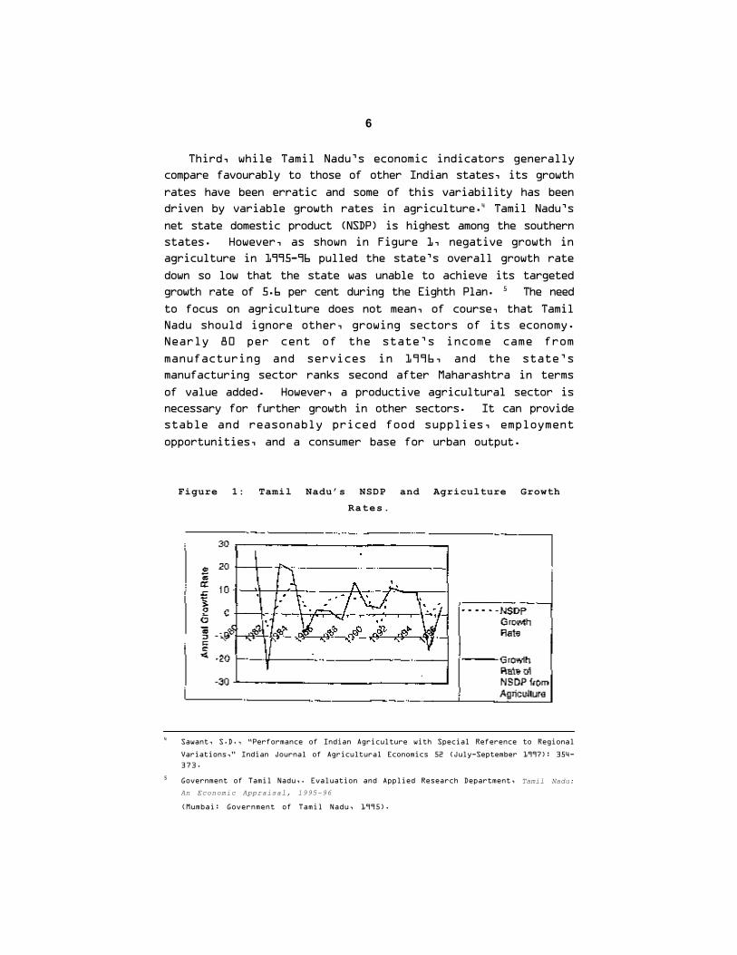
Third, while Tamil Nadu’s economic indicators generallycompare favourably to those of other Indian states, its growth

rates have been erratic and some of this variability has beendriven by variable growth rates in agriculture.4 Tamil Nadu’s

net state domestic product (NSDP) is highest among the southernstates. However, as shown in Figure 1, negative growth inagriculture in 1995-96 pulled the state’s overall growth rate

down so low that the state was unable to achieve its targetedgrowth rate of 5.6 per cent during the Eighth Plan. 5 The need

to focus on agriculture does not mean, of course, that TamilNadu should ignore other, growing sectors of its economy.Nearly 80 per cent of the state’s income came from

manufacturing and services in 1996, and the state’smanufacturing sector ranks second after Maharashtra in terms

of value added. However, a productive agricultural sector isnecessary for further growth in other sectors. It can providestable and reasonably priced food supplies, employment

opportunities, and a consumer base for urban output.

Figure 1: Tamil Nadu’s NSDP and Agriculture GrowthRates.

4 Sawant, S.D., “Performance of Indian Agriculture with Special Reference to Regional

Variations,” Indian Journal of Agricultural Economics 52 (July-September 1997): 354-373.

5 Government of Tamil Nadu,. Evaluation and Applied Research Department, Tamil Nadu:An Economic Appraisal, 1995-96

(Mumbai: Government of Tamil Nadu, 1995).

7

Fourth, Tamil Nadu has high rural poverty rates, and in

order to raise incomes in the agricultural sector, it must raise

agricultural productivity. In 1994, Tamil Nadu’s NSDP per

capita was the highest among India’s southern states and fifth

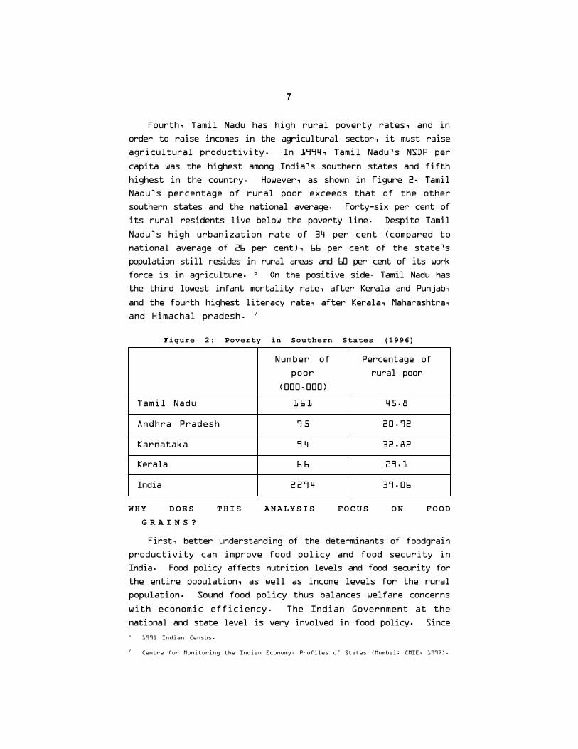
highest in the country. However, as shown in Figure 2, Tamil

Nadu’s percentage of rural poor exceeds that of the other

southern states and the national average. Forty-six per cent of

its rural residents live below the poverty line. Despite Tamil

Nadu’s high urbanization rate of 34 per cent (compared to

national average of 26 per cent), 66 per cent of the state’s

population still resides in rural areas and 60 per cent of its work

force is in agriculture. 6 On the positive side, Tamil Nadu has

the third lowest infant mortality rate, after Kerala and Punjab,

and the fourth highest literacy rate, after Kerala, Maharashtra,

and Himachal pradesh. 7

Figure 2: Poverty in Southern States (1996)

Number of Percentage of

poor rural poor

(000,000)

Tamil Nadu 161 45.8

Andhra Pradesh 95 20.92

Karnataka 94 32.82

Kerala 66 29.1

India 2294 39.06

WHY DOES THIS ANALYSIS FOCUS ON FOODG R A I N S ?

First, better understanding of the determinants of foodgrain

productivity can improve food policy and food security in

India. Food policy affects nutrition levels and food security for

the entire population, as well as income levels for the rural

population. Sound food policy thus balances welfare concerns

with economic efficiency. The Indian Government at the

national and state level is very involved in food policy. Since6 1991 Indian Census.

7 Centre for Monitoring the Indian Economy, Profiles of States (Mumbai: CMIE, 1997).

8

1943, India has employed considerable food control, such as

input subsidies, international and domestic trade restrictions,

and subsidized distribution through the Public Distribution

System8.

Indian Food Policy Objectives Concerning Foodgrains

1. Achieve self-sufficient in production.

2. Maintain price stability.

3. Assure equitable distribution of supply at

reasonable prices.

In recent years, food policy experts have expressed con-

cern that farmers are shifting from foodgrain to non-foodgrain

production, and that India will thus be unable to meet its

growing foodgrain needs through domestic production. The

1990s marked a distinct fall in the growth of foodgrains in

India to a rate barely equal to population growth. The

Government of India has recognized this trend as a concern

that “must be reversed.”9 The shift away from foodgrains

reflects farmers’ changing production incentives and highlights

the need for policy makers to better understand farmers’

production decisions. This report uses a production function

approach to model the effects of geography on farmers’

production decisions.

Second, the majority of agricultural land in India is devoted

to foodgrains, so productivity in foodgrains is often used as a

proxy for agricultural productivity. As shown in Figure 3, well

over 50 per cent of the gross cropped area in all but 3 states

is under foodgrain cultivation.

8 For further information on Indian food policy see Chopra, R.N., Evolution of Food

Policy in India (New Delhi: Macmillan India Ltd., 1981) and Sanderson, Fred and Shyamal

Roy, Food Trends and Prospects in India (Washington, DC: Brookings Institution, 1979).

Policy analysts disagree as to whether India’s food policy favours poor consumers,

urban consumers, large farm holders and/or powerful farm lobbies, and whether it

supports or hinders agricultural productivity.9 Government of India, Economic Survey 1998-99 (New Delhi: Government of India,

Ministry of Finance Economic Division, 1999) 117.

9

OTHER ANALYSIS OF AGRICULTURAL PRODUCTIVITYIN INDIA.

Most economic Analysis of Indian agriculture to date focus

on non-geographic factors, such as economic policies on

subsidies and tariffs; Green Revolution technology; or

institutional constraints, such as access to credit.10 There have

been some attempts to incorporate geography into economic

Analysis of agriculture in India. Under the leadership of

SN. Subramanium, the Madras Institute began studying

geography and agriculture in India as early as 1928. Until the

Green Revolution in the 1960s, however, the studies focussed

on descriptive accounts of static land use and crop distribution.

Since the 1960s, there has been increased interest in

regional disparities in agricultural development and crop

productivity. Most studies argue that policies and technology

are the key factors driving regional variations in agriculture.11

In 1979, a study by the Brookings Institution argued that the

largest variations in agricultural performance in the 1960s-70s

were due to the cost of technology and to technology’s poor

adaptation to geographic conditions.12 These studies, however,

tend to control for the fixed effects of geography in order to

focus on other determinants of agricultural productivity. There

10 Tiwari, P.S., Agricultural Geography (New Delhi: Heritage Publishers, 1986).

11 Chatterjee, S.P., Fifty years of Science in India: Progress of Geography, (Calcutta:Indian Science Congress Association, 1968).

12 Sanderson and Roy.

Figure 3: Percentage of Gross Cropped area (GCA) inFoodgrains

10

have been few efforts to control for other determinants to

examine the effects of geographic variations on agricultural

productivity across Indian states.

TAMIL NADU IS AN IDEAL CASE STUDY

Tamil Nadu’s unique geography makes it an ideal region in

which to apply cross-state analysis of the implications of

geography on agricultural productivity on India. It is the

southern most state in India, and ninety-five per cent of the state

is in the tropics.

Tamil Nadu’s northern and western boundaries are flanked

by the Western Ghats, which reach a peak of 8,000 feet in the

Nilgiri Hills. The southern and eastern boundaries of the state

are on the Indian Ocean. Most of the south-eastern portion is

comprised of plains with one major river and several small

tributaries.

Due to its unique location, Tamil Nadu is the only state in

India that receives two monsoons. From June until September,

it receives the southwest monsoon, on which most of the state’s

agriculture relies. On average, the state receives 32.4 per cent

of its annual rainfall during this season. From October to

December, it receives the northeast monsoon, from which it

receives 47.6 per cent of its annual rainfall. Tamil Nadu’s

annual rainfall average is low to moderate at 943 mm per year.

Its tropical climate, and temperatures ranging from 180C to 440C

makes the rate of surface water run off and evaporation very

high. Therefore, it is difficult to store monsoon rains in tanks.

Despite the state’s considerable investment in expansion of

groundwater irrigation, ground water tables are rapidly

decreasing.

OVERVIEW OF THE PAPER

The remainder of this report is organized in six sections.

Section II describes project methodology and useful tools for

further analysis. Section III gives an overview of regional

foodgrain trends in rice, wheat, maize, and total foodgrains since

the Green Revolution. It also provides a closer look at foodgrain

11

trends in Tamil Nadu. Section IV Analysis how state variations

in foodgrain yields correspond with five geographic variables in

India and isolates Koeppen Climate Zones as the geographic

variable of interest for this study. Section V presents two

empirical models that isolate the impact of geography on state

foodgrain yields in India. These models hold constant income,

agricultural inputs, and technology. Section VI describes a

preliminary analysis of how input levels and other factors of

production differ across Koeppen Zones. Finally, this report

concludes with six recommendations for the Tamil Nadu

Government incorporate the policy implications of these findings.

12

II. METHODS AND TOOLS

Step 1: Building the data set

This study combines two data sources from HIID, the

Integrated India Data Set and Geographic Information Systems

(GIS) India project files.13 The combined Integrated Data Set

now includes over 100 economic, demographic and geographic

variables for each state and most union territories from

1980-1996. In addition, this study uses the World Bank’s India

Agricultural Data Set. This data set includes district level data

for 271 districts in 13 states, covering 85 per cent of India for

the period 1967-1986. Kerala and Assam are the two major

agricultural states not covered. Because this project was

intended to focus on cross-state analysis for the whole country,

a significant portion of the project involved building the

Integrated Data Set to include more agricultural and geographic

variables.

New Agricultural Variables in the Integrated Data Set: Newdata was added for total foodgrain yield per hectare; rice, wheat

and maize yields; area under foodgrain cultivation; tractors;

electric pumps; diesel pumps; fertilizer; average rainfall per year;

net and gross irrigated area under rice, wheat, maize and total

foodgrain cultivation; cultivable land; and land sown.14

New Geographic Variables in the Integrated Data Set: UsingGIS, data tables were built from Maps of India and added to

the data set. The new data included measures for mean eleva-

tion (meters), surface temperature (average of monthly means

13 The Geographic Information Systems India Project file was built by Andrew Mellinger of

HIID. He contributed greatly to this project by providing expert assistance in working

with GIS.

14 The majority of the new agricultural data was drawn three publications by the Govern-

ment of India, the Centre for Monitoring the Indian Economy, Agriculture, August 1997edition (Mumbai: CMIE, 1997); Economic Intelligence Service, Agriculture (Mumbai: Eco-nomic Intelligence Service, September 1998); and Ministry of Agriculture, Area andProduction of Principal Crops in India (New Delhi: Ministry of Agriculture, 1994). Recentdata was also used from Ministry of Agriculture, Agricultural Statistics at a Glance (NewDelhi: Image Print, March 1998) and Ministry of Agriculture, Indian Agriculture in Brief26th edition (New Delhi: Government of India Press, May 1995).

13

in 1987), rainfall (monthly mean for 1987), Koeppen Zones15

(percentage of land area in each zone), distance to the nearest

coastline (in km from the centroid), soil moisture (mean), soil

temperature (mean), soil depth (mean), soil suitability (mean),

irrigation suitability (mean) and Matthews Cultivated Land.

Limitations of the Integrated Data Set

The main weakness in using the Integrated Data Set to

study geography and agriculture is that it lacks adequate rain,

temperature and soil data for varying years. For example, the

only temperature and precipitation data included are the

monthly means for 1987, a drought year in India. HIID is in

the process of coding almost 100 years of precipitation and

temperature data from meteorological stations. This data will

prove valuable in future Analysis. In addition, the Integrated

Data Set’s only soil data are two soil suitability indices for all

crops, making detailed foodgrain analysis difficult. In order to

remedy the weaknesses of the Integrated Data Set, World Bank’s

district level data set was used as well.

The World Bank India Agricultural Data Set

The World Bank Data Set includes detailed agro-climatic

data on temperature, rainfall, and soil quality. It also includes

statistics on agricultural productivity, inputs, technology use, and

prices for 1967-1986. Climate data is from meteorological

climate and precipitation observations from 160 weather stations

across India and is calculated for districts in the set using surface

interpolation techniques.16

15 Koeppen Zones are a climate classification system. See Appendix B for a guide to Koeppen

Zone classification.

16 Much of the work on this data set was originally organized by Robert Evenson with

James McKinsey. The data set has been used extensively by the Word Bank in Studying

the effects of climate change on Indian Agriculture. For more information on World

Bank analysis using the World Bank Data Set, edaphic variables, and extrapolating

climate data from station to district level, see Dinar, Ariel, et al, Measuring the Impactof Climate Change on Indian Agriculture (Washington, DC: World Bank, 1998), WorldBank Technical Paper No. 402. The World Bank India Agricultural Data Set may be

downloaded from http://www-esd.worldbank.org/indian/database.heml.

14

Step 2: Identifying patterns using Geographic Informa-tion Systems

In addition to its use in providing geographic data for the

Integrated Data Set, GIS is also valuable as a tool of analysis

in its own right. In this study, it was useful in illustrating trends

and correlations between geographic and foodgrain yield

variations among states. These are complex relationship that

are often difficult to study through the use of statistics alone.

GIS maps helped isolate India’s Koeppen Zones as the key

geographic variable of interest in this project. Appendix A

includes sample GIS maps.

Step 3: Designing an Empirical Model

Building on a literature review and GIS results, this study

undertook a formal empirical analysis of the effect of geography

on foodgrain yields. The underlying hypothesis tested was that

dry Koeppen Zones have the most positive effect on foodgrain

yields, even when income, Green Revolution technology, and

inputs are held constant. The focus was on yields because most

analysis agree that, due to limited resources, increased

production in India will only come through increased yields.

This hypothesis was tested in sequential steps. The following

sections of this report mirror these steps. First, is there regional

variation in foodgrain yields in India? Second, do foodgrain

yields vary with India’s geographic variation? In this step,

Koeppen Zones were identified as the geographic variable of

interest. Third, holding other factors of production constant,

do Koeppen Zones have different effects on foodgrain yields?

Fourth, is there any evidence that non-geographic factors of

production are affected by Koeppen Zones?

The empirical methods used include t-tests of the equality

of means to measure whether yields and variables differ in a

statistically significant manner across Koeppen Zones; linear

regression analysis; F-tests and t-tests of coefficient estimates; and

predictions and simulations using the results of regression

analysis. The regression models follow Gallup in using an

agricultural production function to explain the empirical

15

relationship between inputs, geography and agricultural

productivity. The dependent variables were rice, wheat, maize,

and total foodgrain yields.

The production function model was chosen because it works

best in isolating the effects of geographic variables on the

dependent variable. Many recent Analysis have followed the

Ricardian model, using annual net revenue as a proxy for net

rent or value of farmland. Net revenues are used because

land rents are so highly controlled. However, net revenues

can only serve as estimates and may thus distort results.17 Other

work controls for differences in geography with fixed effects.

This, however, nets out the influence of geography from the

analysis.18

In contrast to other models, the use of a physical production

function in Gallup’s words “avoids most of the complications of

the effect of the economic policy regime on agriculture, like

exchange rates, quotas, price subsidies and taxes. Nor should

missing markets affect the estimation. Whatever input levels are

chosen, which will be affected by price distortions and marketimperfections, those inputs should have a consistent impact on

output if the aggregate production function specification is

tenable.”19

One drawback to the use of the production function

approach is that it does not directly estimate policy effects within

the model. However, direct measurement of policy effects in

the empirical model are problematic in any case because

comprehensive data on policy variables is often unavailable.

Also, there is little variation in policy across states as many

agriculture-related policies are determined on a national basis

17 For further explanation, see Dinar, Ariel et al, Measuring the Impact of Climate Change

on Indian Agriculture (Washington, DC: World Bank, March 1998), World Bank Tech-nical Paper No. 402. Another weakness of the Ricardian approach is that it will be

biased if an uncontrolled factor is correlated with the variable of interest. Thus, it

becomes especially important to measure and control for every variable that might affectfarm economic performance and be correlated with geographic variables. This can

often be difficult because of the dearth of data on developing countries.

18 Gallup, 1.

19 Gallup, 2.

16

in India. Advocates of the Ricardian method argue that using

a production function may overstate the effects of geography.

Nevertheless, the production function approach is ideal for this

analysis because it allows for estimation of the isolated effects

of geography on yields.

17

III. REGIONAL FOODGRAIN TRENDS

Question: Is there regional variation in foodgrain yields in

India?

Answer: Yes, foodgrain yields vary considerably across Indian

states. In particular, the early years of the Green

Revolution marked a period of pronounced regional

variation in foodgrain yields between the Northwest

and the South. Regional variation in yields has

decreased since the 1980 but is still apparent.

National Trends (1967-1980)

The Green Revolution in the late 1960s shifted the world’s

focus from increasing agricultural output through expansion of

cultivated area to increasing it through higher yields. Yields

were increased through the use of irrigation, fertilizer and new

high yield variety seeds (HYVs). From 1966 to 1980, India

increased its foodgrain yields by 63 per cent from 644 kg/ha

to 1,023 kg/ha. The 1970s thus began India’s move towards

self-sufficiency in foodgrains.

The revolutionary improvements of the 1970s, however, also

began more pronounced variation in foodgrain yields between

the Northwest and the South. Output growth in 1970s was

heavily concentrated in the Northwest regions of Punjab,

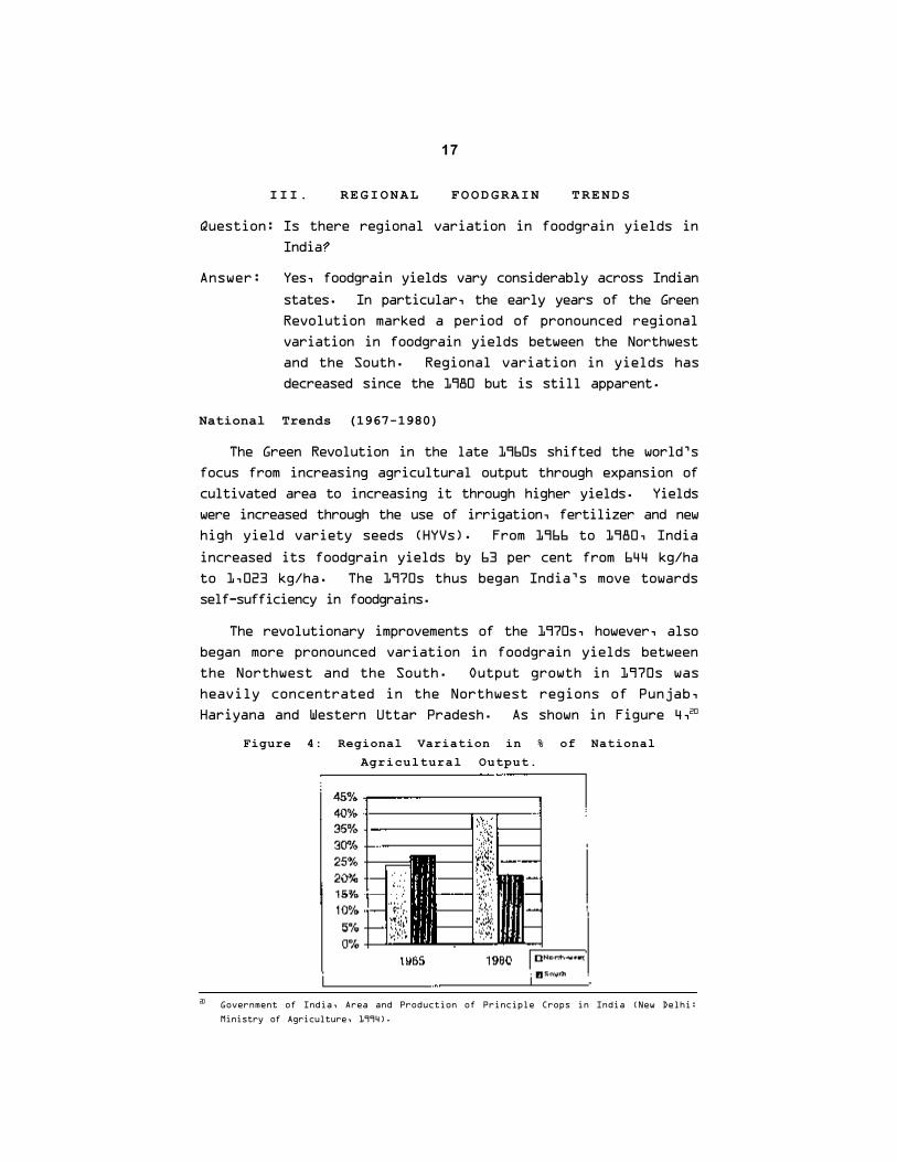
Hariyana and Western Uttar Pradesh. As shown in Figure 4,20

Figure 4: Regional Variation in % of NationalAgricultural Output.

20 Government of India, Area and Production of Principle Crops in India (New Delhi:

Ministry of Agriculture, 1994).

18

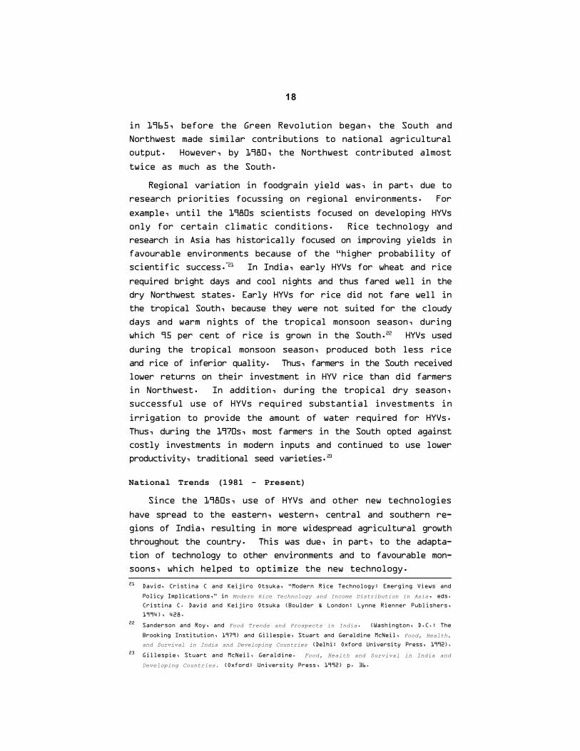
in 1965, before the Green Revolution began, the South and

Northwest made similar contributions to national agricultural

output. However, by 1980, the Northwest contributed almost

twice as much as the South.

Regional variation in foodgrain yield was, in part, due to

research priorities focussing on regional environments. For

example, until the 1980s scientists focused on developing HYVs

only for certain climatic conditions. Rice technology and

research in Asia has historically focused on improving yields in

favourable environments because of the “higher probability of

scientific success.”21 In India, early HYVs for wheat and rice

required bright days and cool nights and thus fared well in the

dry Northwest states. Early HYVs for rice did not fare well in

the tropical South, because they were not suited for the cloudy

days and warm nights of the tropical monsoon season, during

which 95 per cent of rice is grown in the South.22 HYVs used

during the tropical monsoon season, produced both less rice

and rice of inferior quality. Thus, farmers in the South received

lower returns on their investment in HYV rice than did farmers

in Northwest. In addition, during the tropical dry season,

successful use of HYVs required substantial investments in

irrigation to provide the amount of water required for HYVs.

Thus, during the 1970s, most farmers in the South opted against

costly investments in modern inputs and continued to use lower

productivity, traditional seed varieties.23

National Trends (1981 - Present)

Since the 1980s, use of HYVs and other new technologies

have spread to the eastern, western, central and southern re-

gions of India, resulting in more widespread agricultural growth

throughout the country. This was due, in part, to the adapta-

tion of technology to other environments and to favourable mon-

soons, which helped to optimize the new technology.

21 David, Cristina C and Keijiro Otsuka, “Modern Rice Technology: Emerging Views and

Policy Implications,” in Modern Rice Technology and Income Distribution in Asia, eds.Cristina C. David and Keijiro Otsuka (Boulder & London: Lynne Rienner Publishers,

1994), 428.22 Sanderson and Roy, and Food Trends and Prospects in India. (Washington, D.C.: The

Brooking Institution, 1979) and Gillespie, Stuart and Geraldine McNeil, Food, Health,and Survival in India and Developing Countries (Delhi: Oxford University Press, 1992).

23 Gillespie, Stuart and McNeil, Geraldine. Food, Health and Survival in India and

Developing Countries. (Oxford: University Press, 1992) p. 36.

19

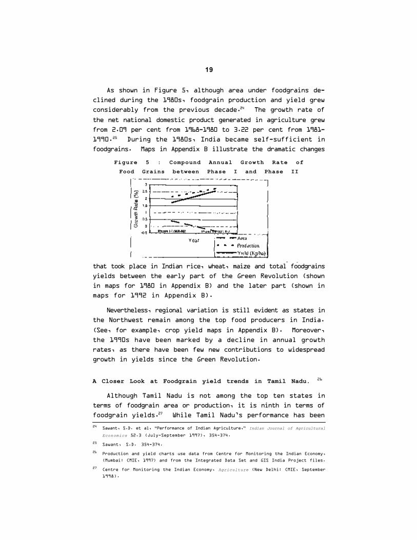
As shown in Figure 5, although area under foodgrains de-

clined during the 1980s, foodgrain production and yield grew

considerably from the previous decade.24 The growth rate of

the net national domestic product generated in agriculture grew

from 2.09 per cent from 1968-1980 to 3.22 per cent from 1981-

1990.25 During the 1980s, India became self-sufficient in

foodgrains. Maps in Appendix B illustrate the dramatic changes

that took place in Indian rice, wheat, maize and total foodgrains

yields between the early part of the Green Revolution (shown

in maps for 1980 in Appendix B) and the later part (shown in

maps for 1992 in Appendix B).

Nevertheless, regional variation is still evident as states in

the Northwest remain among the top food producers in India.

(See, for example, crop yield maps in Appendix B). Moreover,

the 1990s have been marked by a decline in annual growth

rates, as there have been few new contributions to widespread

growth in yields since the Green Revolution.

A Closer Look at Foodgrain yield trends in Tamil Nadu. 26

Although Tamil Nadu is not among the top ten states in

terms of foodgrain area or production, it is ninth in terms of

foodgrain yields.27 While Tamil Nadu’s performance has been

24 Sawant, S.D. et al, “Performance of Indian Agriculture,” Indian Journal of Agricultural

Economics 52.3 (July-September 1997), 354-374.

25 Sawant, S.D. 354-374.

26 Production and yield charts use data from Centre for Monitoring the Indian Economy,

(Mumbai: CMIE, 1997) and from the Integrated Data Set and GIS India Project files.

27 Centre for Monitoring the Indian Economy, Agriculture (New Delhi: CMIE, September1998).

Figure 5 : Compound Annual Growth Rate ofFood Grains between Phase I and Phase II

20

generally positive, there are two causes for concern. First, Tamil

Nadu has had volatile growth rates in foodgrain yields since

the mid-1980s. Second, Tamil Nadu’s principal foodgrain crop,

rice, has had declining growth rates in yield since the mid-1980s.

These trends prompt considerable food security concerns.

Rice comprises nearly 80 per cent of Taml Nadu’s total

foodgrain production. Today, Tamil Nadu is fourth in rice yield

after Punjab, Hariyana and Goa. During the 1980s, Tamil

Nadu’s area under rice cultivation declined by almost 10 per cent

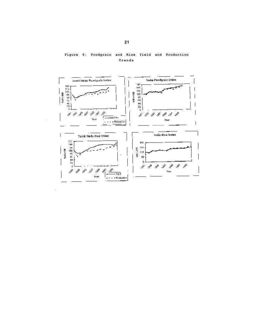
to 2,228.5 ha. in 1994.28 Yield and production levels have

been positive since the 1980s, but the growth rates in yields

are decreasing as shown in Figure 6.

During the 1980s, Tamil Nadu comprised the third largest

share of national value of agricultural output at 9.5 per cent

after Uttar Pradesh and Madhya Pradesh.29 However, the

contribution of agriculture to NSDP declined faster in Tamil

Nadu than in India, from 52 per cent in 1960 to 40 per cent

in 1982, as compared to 49 to 40 per cent over the same period

in India.30

28 Ministry of Agriculture, Area and Production of Principal Crops in India, Volumes

1987-94 (New Delhi: Ministry of Agriculture, 1987-94).

29 Government of Tamil Nadu, Tamil Nadu : An Economic Appraisal, 1995-96 (Chennai:

Government of Tamil Nadu, 1996).

30 Perumalsamy, S. Economic Development of Tamil Nadu (New Delhi: S. Chand and

Company Ltd., 1996).

21

Figure 6: Foodgrain and Rise Yield and ProductionTrends

22

IV. GEOGRAPHIC VARIATION AND FOODGRAINY I E L D S

Question: Do state foodgrain yields vary with India’s geographic

variation?

Answer: Yes, state foodgrain yields vary considerably with

differences in Koeppen Climate Zone classification.

Koeppen Zones serve as a summary variable for

rainfall, temperature and soil quality. States in thedry Koeppen Zone have the highest average

foodgrain yields. Based on statistical analysis and

maps using the Integrated Data Set and GIS India

Project file, this report identifies Koeppen Zones as

the Key variable of interest for further analysis.

Cross-country Analysis done by Sachs and Gallup

have also identified agro-climatic zones as significant

to variation in agricultural productivity.

This section presents a summary of India’s cross-state

foodgrain yield variation across five geographic variables found

in the Integrated Data Set and GIS India Project file: Koeppen

Climate Zone, elevation, average precipitation, distance from the

nearest navigable river and a soil suitability index. (For further

information on these variables, maps and charts, see Appendix

B).

VARIABLE 1: KOEPPEN ZONES

Koeppen Zones are a climate classification system based on

monthly and seasonal rainfall and temperature, and other

geographic indicators. Nine Koeppen sub-zones are represented

in India, but only four make up the majority of land in most of

India’s states. These are the tropical monsoon type AM zone;

the tropical AW zone with a distinct dry season; the dry steppe

climate BS zone and the temperate CW zone with a winter dry

season. (For a guide to the Koeppen classification system,classification of regions by Koeppen Zone and a map of zones

and regions, see Appendix B). Thirty-eight per cent of India is

in the temperate BS zone, 27 per cent in the tropical land falls

within the tropical monsoon AM zone 16 per cent in the dry

BS zone and 6 per cent in the temperate AW zone. More

than 92 per cent of Tamil Nadu’s land falls within the tropical

23

monsoon AM zone. As in HIID’s cross-national studies, regions

with over 50 per cent of their land in one Koeppen Zone were

classified within that zone. Tamil Nadu was thus classified as

“tropical AM”.

Average Yields across Koeppen zones

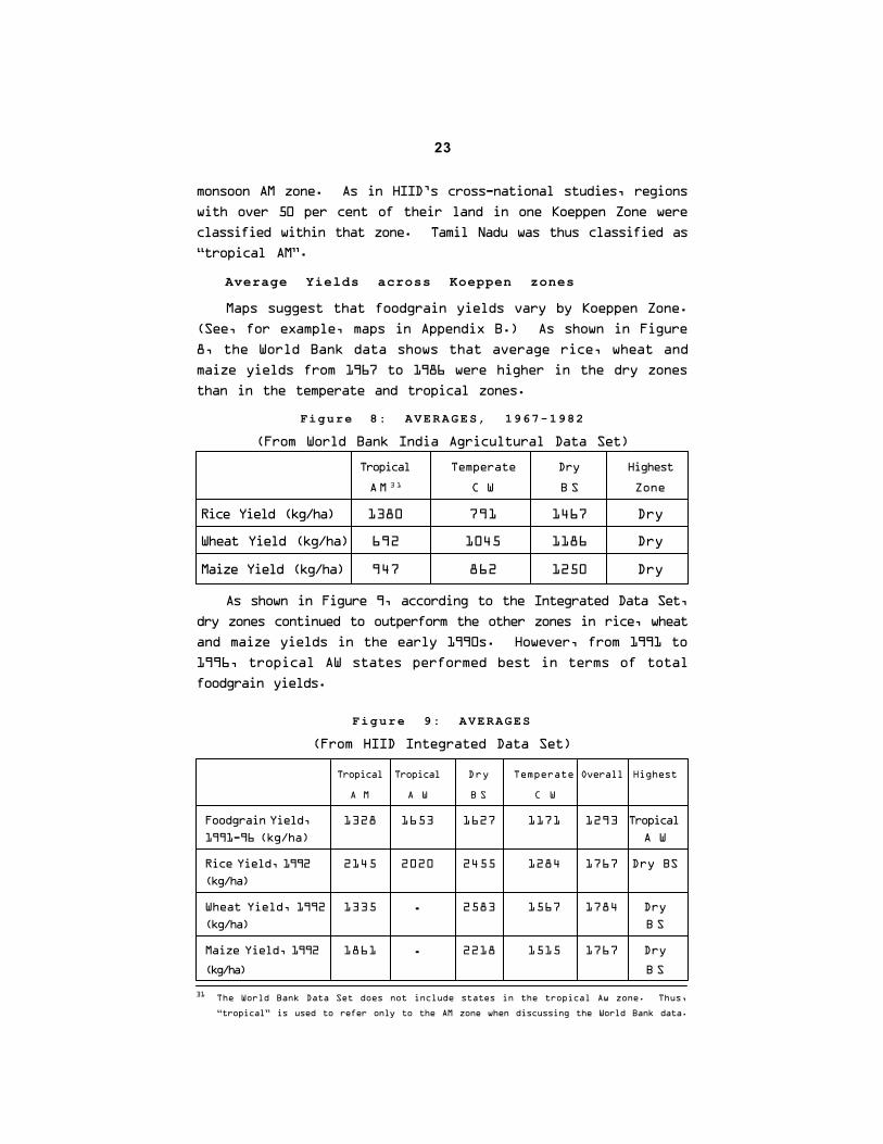
Maps suggest that foodgrain yields vary by Koeppen Zone.

(See, for example, maps in Appendix B.) As shown in Figure

8, the World Bank data shows that average rice, wheat and

maize yields from 1967 to 1986 were higher in the dry zones

than in the temperate and tropical zones.

Figure 8: AVERAGES, 1967-1982

(From World Bank India Agricultural Data Set)

Tropical Temperate Dry Highest

AM 3 1 C W B S Zone

Rice Yield (kg/ha) 1380 791 1467 Dry

Wheat Yield (kg/ha) 692 1045 1186 Dry

Maize Yield (kg/ha) 947 862 1250 Dry

As shown in Figure 9, according to the Integrated Data Set,

dry zones continued to outperform the other zones in rice, wheat

and maize yields in the early 1990s. However, from 1991 to

1996, tropical AW states performed best in terms of total

foodgrain yields.

Figure 9: AVERAGES

(From HIID Integrated Data Set)

Tropical Tropical Dry Temperate Overall Highest

A M A W B S C W

Foodgrain Yield, 1328 1653 1627 1171 1293 Tropical1991-96 (kg/ha) A W

Rice Yield, 1992 2145 2020 2455 1284 1767 Dry BS(kg/ha)

Wheat Yield, 1992 1335 .. 2583 1567 1784 Dry(kg/ha) B S

Maize Yield, 1992 1861 .. 2218 1515 1767 Dry

(kg/ha) B S

31 The World Bank Data Set does not include states in the tropical Aw zone. Thus,

“tropical” is used to refer only to the AM zone when discussing the World Bank data.

24

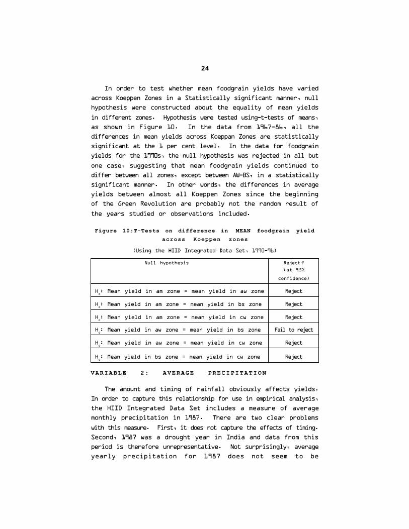
In order to test whether mean foodgrain yields have varied

across Koeppen Zones in a Statistically significant manner, null

hypothesis were constructed about the equality of mean yields

in different zones. Hypothesis were tested using-t-tests of means,

as shown in Figure 10. In the data from 1967-86, all the

differences in mean yields across Koeppan Zones are statistically

significant at the 1 per cent level. In the data for foodgrain

yields for the 1990s, the null hypothesis was rejected in all but

one case, suggesting that mean foodgrain yields continued to

differ between all zones, except between AW-BS, in a statistically

significant manner. In other words, the differences in average

yields between almost all Koeppen Zones since the beginning

of the Green Revolution are probably not the random result of

the years studied or observations included.

Figure 10:T-Tests on difference in MEAN foodgrain yieldacross Koeppen zones

(Using the HIID Integrated Data Set, 1990-96)

Null hypothesis Reject?

(at 95%

confidence)

Ho: Mean yield in am zone = mean yield in aw zone Reject

Ho: Mean yield in am zone = mean yield in bs zone Reject

Ho: Mean yield in am zone = mean yield in cw zone Reject

Ho: Mean yield in aw zone = mean yield in bs zone Fail to reject

Ho: Mean yield in aw zone = mean yield in cw zone Reject

Ho: Mean yield in bs zone = mean yield in cw zone Reject

VARIABLE 2: AVERAGE PRECIPITATION

The amount and timing of rainfall obviously affects yields.

In order to capture this relationship for use in empirical analysis,

the HIID Integrated Data Set includes a measure of average

monthly precipitation in 1987. There are two clear problems

with this measure. First, it does not capture the effects of timing.

Second, 1987 was a drought year in India and data from this

period is therefore unrepresentative. Not surprisingly, average

yearly precipitation for 1987 does not seem to be

25

related to foodgrain yields in the sample. Likewise, the cross-

state temperature data is not informative. Given the limitations

in the current Integrated Data Set, the World Bank India

Agricultural Data Set was used instead to study district level

rainfall and temperature effects.

VARIABLE 3 : ELEVATION

In many countries, cropping patterns are strongly linked with

elevation. For example, in sub-Saharan Africa, one might

observe those at the foot of mountain growing sorghum and

millet while those higher up grow maize, vegetables, and beans.

Aside from the Himalayas in the far north, India has relatively

little variation in elevation. The HIID Integrated Data Set

includes measures of mean elevation across states, based on

GIS calculations. These state-level measures are not correlated

with foodgrain yields. While there may be evidence within states

of the effects of elevation, effects are not captured at the state-

level.

V A R I A B L E 4 : D I S T A N C E T O T H E N E A R E S T N A V I G A B L E

R I V E R

There is considerable variation in the distance from the

centre of each state or union territory to the nearest navigable

river. The average measure for Pondicherry is the closest at

1.15 km, and the farthest is for Jammu & Kashmir at 1189.72

km. One would expect that regions nearest navigable rivers

might have an advantage in agricultural productivity due to

superior sources of water for irrigation and, perhaps, cheaper

access to agricultural inputs because of the case of transport on

navigable rivers. Thus, regions nearest rivers might have higher

yields on average than those farthest from rivers. This

relationship is not supported in the Integrated Data Set, or in

GIS maps. In fact, states farthest from navigable rivers seem to

have higher yields than those that are closer. One possible

explanation is that the distance to the nearest navigable variable

is too imprecise for use at the cross-state level. It is likely that

yields vary considerably within states in areas at different

distances from rivers, but this relationship is not captured in

state-level data.

26

VARIABLE 5: SOIL SUITABILITY INDEX

It is clear that soils are important to agriculture. For

example, one explanation of Africa’s poor agricultural growth is

its poor soils. The Integrated Data Set includes two indices of

Soil Suitability constructed for all crops. Soil Suitability

Index # 2 has been found to be significant in some cross-

country studies. In studying India’s foodgrain yields, however,

this index is found to be too aggregated to be at use. As the

chart in Appendix B illustrates, states with the lowest soil

suitability values have yields that are about the same as states

with the highest suitability values.

27

32 In the equation, Y is the dependent variable, d is the constant term, Bx are the co

efficients to be estimated, and E is the error term.

V. A MODEL OF GEOGRAPHY AND FOODGRAINY I E L D S

Question: Holding other factors of production constant, do

Koeppen Zones have different effects on foodgrain

yields?

Answer: Yes, Koeppen Zones have different effects on

foodgrain yields. In India, dry and tropical zones

have more positive effects than temperate zones.

Using two empirical models that isolate the impact

of geography on state foodgrain yields in India, this

section shows that rain temperature and soils are

important factors in agricultural productivity. It also

shows that the agro-climatic conditions of dry and

tropical zones have significantly more positive effects

than those of temperate zones in India. Detailed

rainfall and temperature analysis suggest that the

temperate zone’s more volatile precipitation levels

may help to explain why its yields are lowest.

This section presents two empirical models of foodgrain yield

using the HIID Integrated Data Set and the World Bank India

Agricultural Data Set. For each model, regression results are

findings are presented, along with analysis of what drives

simulated differences in mean yields between Koeppan Zones.

The first model isolates the effects of Koeppen Zones on yields.

The second model isolates the effects of rainfall and temperature

across Koeppen Zones.

MODEL #1: ISOLATING THE EFFECTS OF KOEPPENZONES ON YIELDS

Using the HIID Integrated Data Set, the model that provides

the best fit for total foodgrain yield in 1991 includes measures

for rural labor density, fertilizer use, NSDP in 1980 and the four

primary Koeppen Zones represented in India. This model,

shown in Figure 11,32 has an R2 value of 0.995 and an adjusted

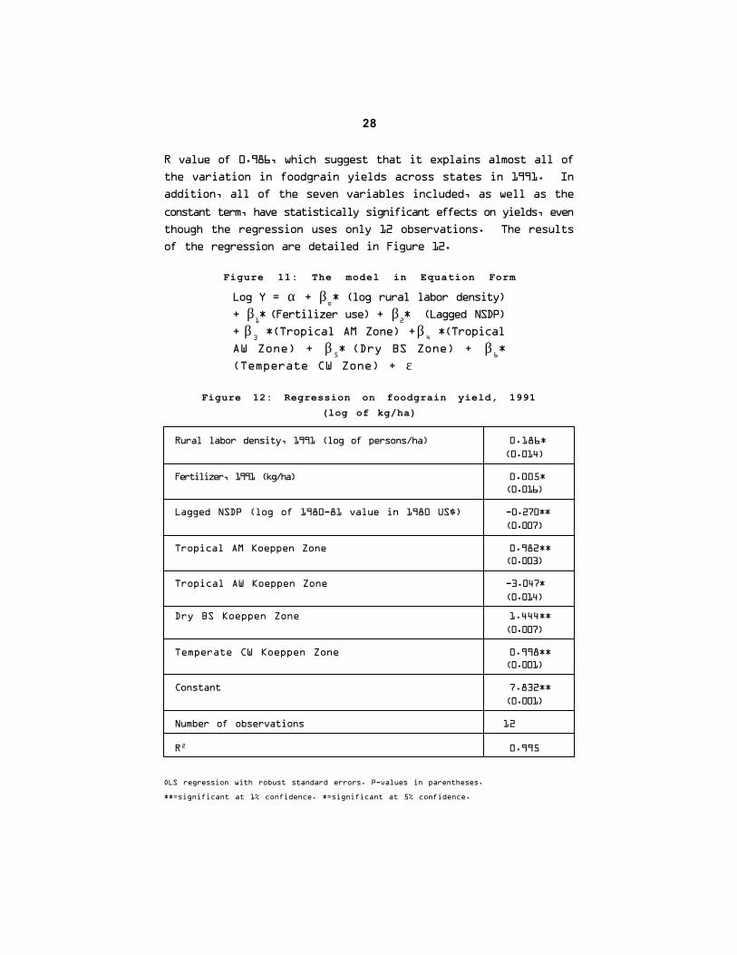
28

R value of 0.986, which suggest that it explains almost all of

the variation in foodgrain yields across states in 1991. In

addition, all of the seven variables included, as well as the

constant term, have statistically significant effects on yields, even

though the regression uses only 12 observations. The results

of the regression are detailed in Figure 12.

Figure 11: The model in Equation Form

Log Y = α + βo* (log rural labor density)

+ β1* (Fertilizer use) + β

2* (Lagged NSDP)

+ β3 *(Tropical AM Zone) + β

4 *(Tropical

AW Zone) + β5* (Dry BS Zone) + β

6*

(Temperate CW Zone) + ε

Figure 12: Regression on foodgrain yield, 1991(log of kg/ha)

Rural labor density, 1991 (log of persons/ha) 0.186*(0.014)

Fertilizer, 1991 (kg/ha) 0.005*(0.016)

Lagged NSDP (log of 1980-81 value in 1980 US$) -0.270**(0.007)

Tropical AM Koeppen Zone 0.982**(0.003)

Tropical AW Koeppen Zone -3.047*(0.014)

Dry BS Koeppen Zone 1.444**(0.007)

Temperate CW Koeppen Zone 0.998**(0.001)

Constant 7.832**(0.001)

Number of observations 12

R2 0.995

OLS regression with robust standard errors. P-values in parentheses.

**=significant at 1% confidence. *=significant at 5% confidence.

29

33 In the Integrated Data Set, only 1980 and 1992 yields were available for rice, wheat and

maize.

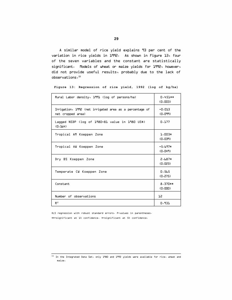
A similar model of rice yield explains 93 per cent of the

variation in rice yields in 1992. As shown in Figure 13, four

of the seven variables and the constant are statistically

significant. Models of wheat or maize yields for 1992, however,

did not provide useful results, probably due to the lack of

observations.33

Figure 13: Regression of rice yield, 1992 (log of kg/ha)

Rural Labor density, 1991 (log of persons/ha) 0.451**(0.003)

Irrigation, 1992 (net irrigated area as a percentage of -0.013net cropped area) (0.099)

Lagged NSDP (log of 1980-81 value in 1980 US$) 0.177(0.164)

Tropical AM Koeppen Zone 1.003*(0.039)

Tropical AW Koeppen Zone -5.697*(0.049)

Dry BS Koeppen Zone 2.687*(0.023)

Temperate CW Koeppen Zone 0.565(0.275)

Constant 8.370**(0.000)


R2 0.931


**=significant at 1% confidence. *=significant at 5% confidence.

30

FINDINGS :

Results suggest that states in the tropical AM zone, like Tamil

Nadu, have an inherent geographic advantage in foodgrain and

rice yields over those in the tropical AW zone, like Kerala.

States in the dry BS zone, however, likely have an advantage

over states in all other zones. The tropical AW zone is clearly

the worst in all cases.

The models using the Integrated Data Set show that most

Koeppen Zone variables have a statistically significant impact

on yields. This might reflect simply that rain, temperature and

soil quality, the measures used in Koeppen Zone classification,

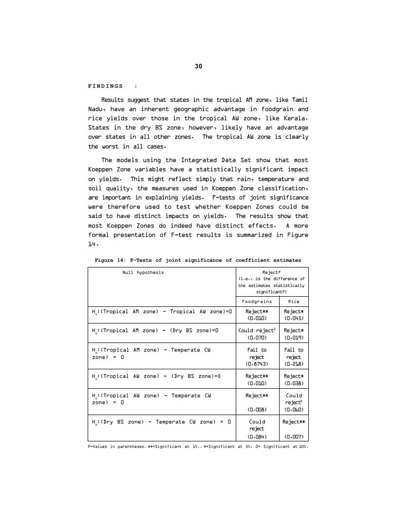
are important in explaining yields. F-tests of joint significance

were therefore used to test whether Koeppen Zones could be

said to have distinct impacts on yields. The results show that

most Koeppen Zones do indeed have distinct effects. A more

formal presentation of F-test results is summarized in Figure

14.

Figure 14: F-Tests of joint significance of coefficient estimates

Null hypothesis Reject?(i.e., is the difference of

the estimates statisticallysignificant?)

Foodgrains Rice

Ho:(Tropical AM zone) - Tropical AW zone)=0 Reject** Reject*

(0.010) (0.045)

Ho:(Tropical AM zone) - (Dry BS zone)=0 Could reject0 Reject*

(0.070) (0.019)

Ho:(Tropical AM zone) - Temperate CW Fail to Fail to

zone) = 0 reject reject(0.8743) (0.218)

Ho:(Tropical AW zone) - (Dry BS zone)=O Reject** Reject*

(0.010) (0.038)

Ho:(Tropical AW zone) - Temperate CW Reject** Could

zone) = 0 reject0

(0.008) (0.060)

Ho:(Dry BS zone) - Temperate CW zone) = 0 Could Reject**

reject

(0.084) (0.007)

P-Values in parentheses. **=Significant at 1%.. *=Significant at 5%. 0= Significant at 10%.

31

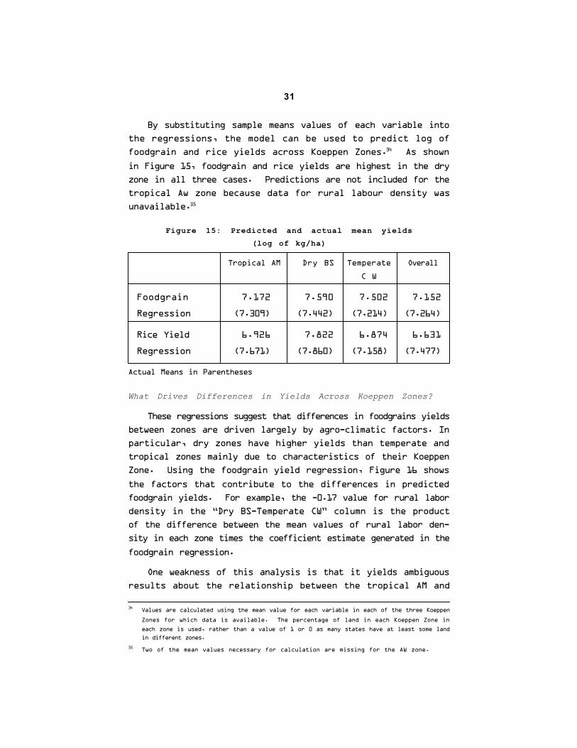
By substituting sample means values of each variable into

the regressions, the model can be used to predict log of

foodgrain and rice yields across Koeppen Zones.34 As shown

in Figure 15, foodgrain and rice yields are highest in the dry

zone in all three cases. Predictions are not included for the

tropical Aw zone because data for rural labour density was

unavailable.35

Figure 15: Predicted and actual mean yields(log of kg/ha)

Tropical AM Dry BS Temperate Overall

C W

Foodgrain 7.172 7.590 7.502 7.152

Regression (7.309) (7.442) (7.214) (7.264)

Rice Yield 6.926 7.822 6.874 6.631

Regression (7.671) (7.860) (7.158) (7.477)

Actual Means in Parentheses

What Drives Differences in Yields Across Koeppen Zones?

These regressions suggest that differences in foodgrains yields

between zones are driven largely by agro-climatic factors. In

particular, dry zones have higher yields than temperate and

tropical zones mainly due to characteristics of their Koeppen

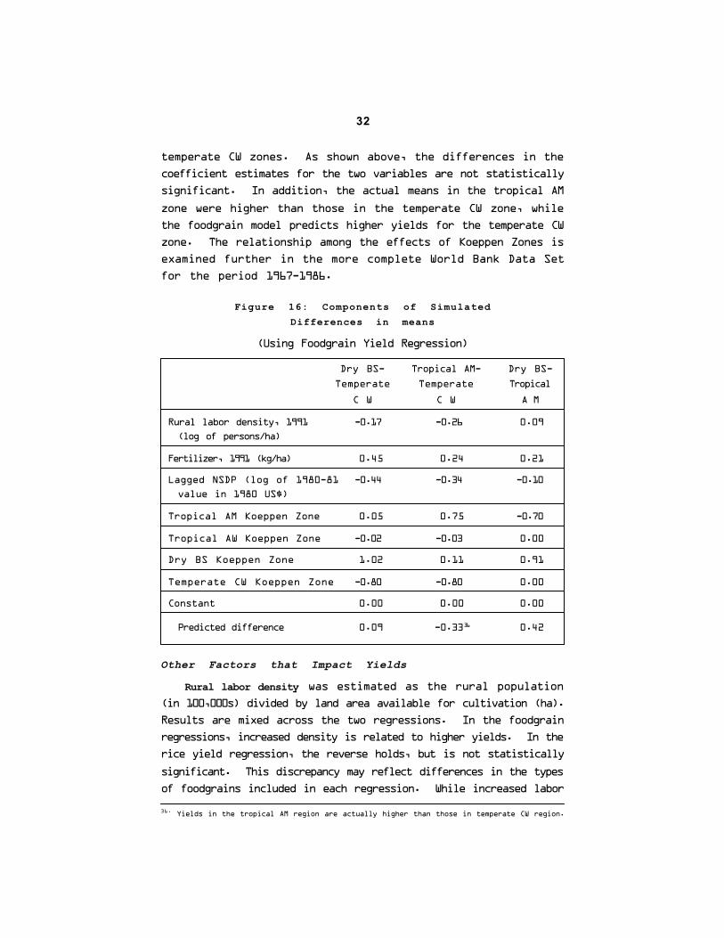
Zone. Using the foodgrain yield regression, Figure 16 shows

the factors that contribute to the differences in predicted

foodgrain yields. For example, the -0.17 value for rural labor

density in the “Dry BS-Temperate CW” column is the product

of the difference between the mean values of rural labor den-

sity in each zone times the coefficient estimate generated in the

foodgrain regression.

One weakness of this analysis is that it yields ambiguous

results about the relationship between the tropical AM and

34 Values are calculated using the mean value for each variable in each of the three Koeppen

Zones for which data is available. The percentage of land in each Koeppen Zone in

each zone is used, rather than a value of 1 or 0 as many states have at least some landin different zones.

35 Two of the mean values necessary for calculation are missing for the AW zone.

32

temperate CW zones. As shown above, the differences in the

coefficient estimates for the two variables are not statistically

significant. In addition, the actual means in the tropical AM

zone were higher than those in the temperate CW zone, while

the foodgrain model predicts higher yields for the temperate CW

zone. The relationship among the effects of Koeppen Zones is

examined further in the more complete World Bank Data Set

for the period 1967-1986.

Figure 16: Components of SimulatedDifferences in means

(Using Foodgrain Yield Regression)

Dry BS- Tropical AM- Dry BS-

Temperate Temperate Tropical

C W C W A M

Rural labor density, 1991 -0.17 -0.26 0.09(log of persons/ha)

Fertilizer, 1991 (kg/ha) 0.45 0.24 0.21

Lagged NSDP (log of 1980-81 -0.44 -0.34 -0.10value in 1980 US$)

Tropical AM Koeppen Zone 0.05 0.75 -0.70

Tropical AW Koeppen Zone -0.02 -0.03 0.00

Dry BS Koeppen Zone 1.02 0.11 0.91

Temperate CW Koeppen Zone -0.80 -0.80 0.00

Constant 0.00 0.00 0.00

Predicted difference 0.09 -0.3336 0.42

Other Factors that Impact Yields

Rural labor density was estimated as the rural population(in 100,000s) divided by land area available for cultivation (ha).

Results are mixed across the two regressions. In the foodgrain

regressions, increased density is related to higher yields. In the

rice yield regression, the reverse holds, but is not statistically

significant. This discrepancy may reflect differences in the types

of foodgrains included in each regression. While increased labor

36. Yields in the tropical AM region are actually higher than those in temperate CW region.

33

density may be related to decreased rice yields, for example, it

might have the opposite effect for other foodgrain crops.

Fertilizer and irrigation were used as a rough estimateof agricultural inputs and technology.37 Fertilizer has a positive

impact on foodgrain yields for states in any zone. The results

for irrigation in the rice regression are not statistically signifi-

cant. This may be due to the large proportion of rain-fed ir-

rigation in India, the effects of which will be picked up by the

Koeppen Zone variables. In rice regressions, fertilizer use was

unpredictive, but irrigation levels were useful in the model. This

difference may be due to a variety of factors including lower

requirements for fertilizer in rice cultivation and higher require-

ments for irrigation, or lower responsiveness of modern rice

varieties, as compared to other foodgrains, to fertilizer use.

Lagged NSDP was included in both regressions in order

to account for the effects of income levels across states, and the

1980 NSDP value was used instead of the current figure to

avoid the problem of reverse causality.38 In the foodgrain model,

lagged NSDP has a significant and negative relationship with

yields. The negative relationship might seem to run counter to

conventional wisdom that richer states are better able to afford

technology and inputs to agriculture making for higher yields.

However, it might be explained in that richer states may have

shifted resources from agriculture to manufacturing or services

and raised the costs of labor and capital for agriculture. Lagged

NSDP may, in fact, have a positive effect on yield per person,

even though it has a negative value for yield per hectare, the

measure used here.

37. See, for example, Sanderson and Roy, “Fertilizers, HYVs and irrigation were found to

be highly intercorrelated, so fertilizers are used as a proxy variable to represent the

entire package of modern technological,” p.22.

38. As foodgrain production clearly contributes to NSDP, the NSDP in 1991 is probably a

function of foodgrain productivity in 1991. Thus, the NSDP in 1991 is endogenous,i.e., determined within the model and should not be included in the regression.

34

MODEL #2: ISOLATING THE EFFECTS OF RAINFALLAND TEMPERATURE ACROSS KOEPPEN ZONES

Because adequate rainfall and temperature data are not

available in the HIID Integrated data Set, a similar model was

developed using the World Bank India Agricultural Data Set to

isolate the effects of the different components of Koeppen Zones

on rice, wheat and maize yields during the period 1967-1986.39

The components of Koeppen Zone studied include mean

monthly temperature, mean monthly rainfall, aquifers and soil

type. Model #2 also controlled for non-geographic variables

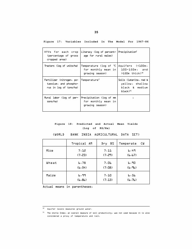
not available in the Integrated Data Set. Figure 17 summa-

rizes the variables used in the best-fit model and Figure 18

shows the actual and predicted mean yields to illustrate that

the model is quite predictive. (For regression results, see

Appendix C).

39. The model generally followed the model for cross-state variations in yield described

above. The regression results are presented in Appendix C.

35

Figure 17: Variables Included In The Model For 1967-86

Figure 18: Predicted and Actual Mean Yields(Log of KG/Ha)

(WORLD BANK INDIA AGRICULTURAL DATA SET)

Tropical AM Dry BS Temperate CW

Rice 7.12 7.11 6.49

(7.23) (7.29) (6.67)

Wheat 6.78 7.06 6.90

(6.54) (7.08) (6.96)

Maize 6.99 7.10 6.56

(6.86) (7.13) (6.76)

Actual means in parentheses.

HYVs for each crop(percentage of grosscropped area)

Tractors (log of units/ha)

Fertilizer (nitrogen, po-tassium, and phospho-rus in log of tons/ha)

Rural labor (log of per-sons/ha)

Literacy (log of percent-age for rural males)

Temperature (log of 0Cfor monthly mean ingrowing season)

Temperature2

Precipitation (log of mmfor monthly mean ingrowing season)

Precipitation2

Aquifers (<100m,100-150m, and>150m thick)40

Soils (laterite, red &yellow, shallowblack & mediumblack)41

..

40 Aquifer levels measures ground water.

41 The storie Index, an overall measure of soil productivity, was not used because it is also

considered a proxy of temperature and rain.

36

Additional Variables Used in Model # 2

Although the models from the two data sets are generally

similar, they differed on certain variables due to the different

data contained in each set. In addition to fertilizers, Model #2

also controlled for HYVs and tractors since so much attention

has been paid to Green Revolution technology in India. Irri-

gation was not controlled for, as the aquifer and precipitation

variables seemed to pick up the effects of India’s groundwater

and rain-fed irrigation. The labor variable in Model# 2 is

weighted by the number of days worked by rural males whose

primary job classification is agricultural labor or cultivation.

Model #2 also controlled for literacy as a proxy for the ability

to adopt new technology. Although infrastructure could im-

prove access to inputs and markets, and thus yields, roads and

distance from sea were found to be insignificant in Model# 2,

and were thus left out of the model.

Temperature and precipitation measurement posed one ofthe biggest challenges in building Model# 2. Cropping calen-

dars contain a complex mix of information that depends not

only on absolute levels, but also on timing, seasons and crop

needs. Temperature and precipitation effects can vary even

between neighbouring farms. The most predictive model used

the log of the monthly mean temperatures and the temperature

squared for each month in the growing season, as well as the

log of the monthly mean precipitation level and the precipita-

tion squard for each month in the growing season. The grow-

ing season is defined when temperature is greater than 50C.42.

A comparison of actual mean crop yields with predicted mean

crop yields shown above illustrates that the model is predic-

tive. Several different methods of including temperature and

precipitation were tested, including the World Bank’s approach

of four evenly spaced months, annual averages, minimums and

maximums, and seasonal averages.

42 Gallup, 4.

37

Temperature and Precipitation Drive Differences inYields across Koeppen Zones.

As in the regression using the Integrated Data Set, the

regressions using the World Bank Data Set show that climate

and precipitation variables have a significant impact on

foodgrain yields in India. In particular, temperature and

precipitation differences across Koeppen Zones appear to be the

largest drivers of rice, wheat, and maize yield differences

between zones. They dry BS zone seems to have the most

favourable temperature and precipitation patterns for all three

crops.

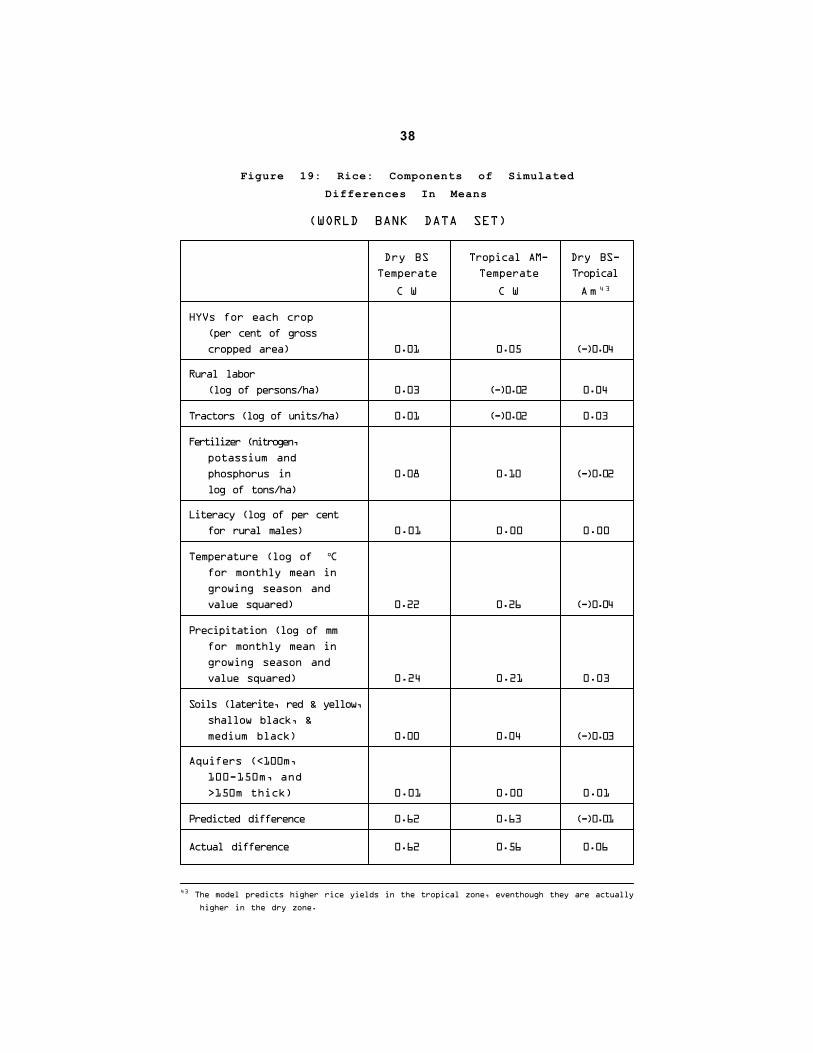
Rice.—As shown in Figure 19, tropical and dry zones have

higher rice yields than temperate zones. Temperature and

precipitation patterns seem largely responsible for this difference.

Dry zones have higher rice yields than tropical zones,

eventhough the model predicts slightly higher tropical yields.

Neither temperature nor precipitation appear to play the most

important role in the difference between tropical and dry zone

yields.

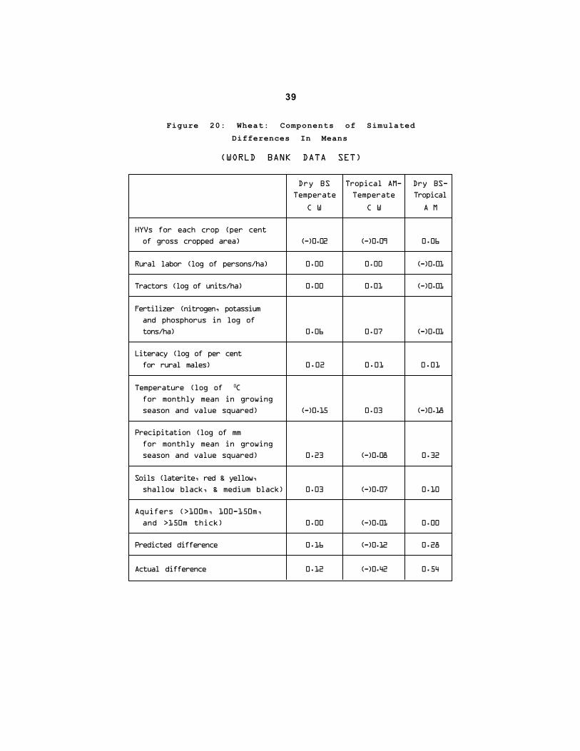
Wheat.— As shown in Figure 20, dry zones have higherwheat yields than temperate zones. Precipitation patters seem

largely responsible for this, despite the favourable temperature

patterns in temperate zones. As expected, tropical zones do

not produce much wheat due to their precipitation patterns.

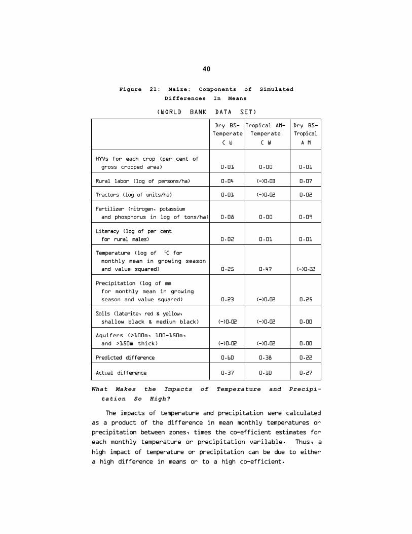
Maize.— As shown in Figure 21, dry zones have highermaize yields than temperate zones. Again, temperature and

precipitation patterns seem largely responsible for this differ-

ence. Tropical zones also have higher maize yields than tem-

perate zones. Temperature patterns seem almost solely respon-

sible for this difference. Dry zones have higher maize yields

than tropical zones. Precipitation patterns seem largely respon-

sible for this difference, despite the favourable temperature

patterns in tropical zones.

38

Figure 19: Rice: Components of SimulatedDifferences In Means

(WORLD BANK DATA SET)

Dry BS Tropical AM- Dry BS-Temperate Temperate Tropical

C W C W Am 4 3

HYVs for each crop(per cent of grosscropped area) 0.01 0.05 (-)0.04

Rural labor(log of persons/ha) 0.03 (-)0.02 0.04

Tractors (log of units/ha) 0.01 (-)0.02 0.03

Fertilizer (nitrogen,potassium andphosphorus in 0.08 0.10 (-)0.02log of tons/ha)

Literacy (log of per centfor rural males) 0.01 0.00 0.00

Temperature (log of oCfor monthly mean ingrowing season andvalue squared) 0.22 0.26 (-)0.04

Precipitation (log of mmfor monthly mean ingrowing season andvalue squared) 0.24 0.21 0.03

Soils (laterite, red & yellow,shallow black, &medium black) 0.00 0.04 (-)0.03

Aquifers (<100m,100-150m, and>150m thick) 0.01 0.00 0.01

Predicted difference 0.62 0.63 (-)0.01

Actual difference 0.62 0.56 0.06

43 The model predicts higher rice yields in the tropical zone, eventhough they are actually

higher in the dry zone.

39

Figure 20: Wheat: Components of SimulatedDifferences In Means


Dry BS Tropical AM- Dry BS-Temperate Temperate Tropical

C W C W A M

HYVs for each crop (per centof gross cropped area) (-)0.02 (-)0.09 0.06

Rural labor (log of persons/ha) 0.00 0.00 (-)0.01

Tractors (log of units/ha) 0.00 0.01 (-)0.01

Fertilizer (nitrogen, potassiumand phosphorus in log oftons/ha) 0.06 0.07 (-)0.01


Temperature (log of 0Cfor monthly mean in growingseason and value squared) (-)0.15 0.03 (-)0.18

Precipitation (log of mmfor monthly mean in growingseason and value squared) 0.23 (-)0.08 0.32

Soils (laterite, red & yellow,shallow black, & medium black) 0.03 (-)0.07 0.10

Aquifers (>100m, 100-150m,and >150m thick) 0.00 (-)0.01 0.00

Predicted difference 0.16 (-)0.12 0.28

Actual difference 0.12 (-)0.42 0.54

40

Figure 21: Maize: Components of SimulatedDifferences In Means


Dry BS- Tropical AM- Dry BS-Temperate Temperate Tropical

C W C W A M

HYVs for each crop (per cent ofgross cropped area) 0.01 0.00 0.01

Rural labor (log of persons/ha) 0.04 (-)0.03 0.07

Tractors (log of units/ha) 0.01 (-)0.02 0.02

Fertilizer (nitrogen, potassiumand phosphorus in log of tons/ha) 0.08 0.00 0.09


Temperature (log of 0C formonthly mean in growing seasonand value squared) 0.25 0.47 (-)0.22

Precipitation (log of mmfor monthly mean in growingseason and value squared) 0.23 (-)0.02 0.25

Soils (laterite, red & yellow,shallow black & medium black) (-)0.02 (-)0.02 0.00

Aquifers (>100m, 100-150m,and >150m thick) (-)0.02 (-)0.02 0.00

Predicted difference 0.60 0.38 0.22

Actual difference 0.37 0.10 0.27

What Makes the Impacts of Temperature and Precipi-tation So High?

The impacts of temperature and precipitation were calculated

as a product of the difference in mean monthly temperatures or

precipitation between zones, times the co-efficient estimates for

each monthly temperature or precipitation varilable. Thus, a

high impact of temperature or precipitation can be due to either

a high difference in means or to a high co-efficient.

41

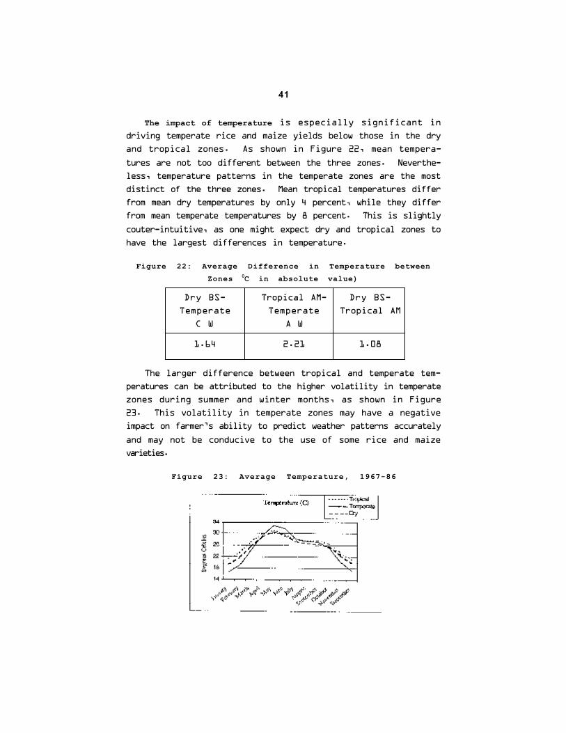
The impact of temperature is especially significant indriving temperate rice and maize yields below those in the dry

and tropical zones. As shown in Figure 22, mean tempera-

tures are not too different between the three zones. Neverthe-

less, temperature patterns in the temperate zones are the most

distinct of the three zones. Mean tropical temperatures differ

from mean dry temperatures by only 4 percent, while they differ

from mean temperate temperatures by 8 percent. This is slightly

couter-intuitive, as one might expect dry and tropical zones to

have the largest differences in temperature.

Figure 22: Average Difference in Temperature betweenZones 0C in absolute value)


Temperate Temperate Tropical AM

C W A W

1.64 2.21 1.08

The larger difference between tropical and temperate tem-

peratures can be attributed to the higher volatility in temperate

zones during summer and winter months, as shown in Figure

23. This volatility in temperate zones may have a negative

impact on farmer’s ability to predict weather patterns accurately

and may not be conducive to the use of some rice and maize

varieties.

Figure 23: Average Temperature, 1967-86

42

The impact of precipitation is especially significant indriving temperate rice, wheat, and maize yields below those in

the dry zones. Precipitation is also significant in driving

temperate rice yields below those in the tropical zone. As with

temperature, a closer look shows that precipitation patterns in

the temperate zones are the most distinct of the three zones as

shown in Figure 24. Mean tropical precipitation differs from

mean dry precipitation by 44 percent, while it differs from mean

temperate precipitation by 35 percent. Again, this is slightly

counter-intuitive, as one might expect dry and tropical zones to

have the largest differences in precipitation.

43

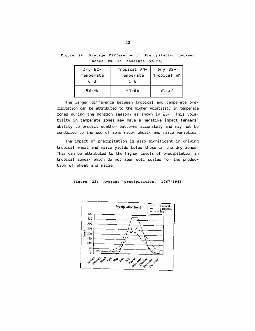
Figure 24: Average Difference in Precipitation betweenZones mm in absolute value)


Temperate Temperate Tropical AM

C W C W

43.46 49.88 39.57

The larger difference between tropical and temperate pre-

cipitation can be attributed to the higher volatility in temperate

zones during the monsson season, as shown in 25. This vola-

tility in temperate zones may have a negative impact farmers’

ability to predict weather patterns accurately and may not be

conducive to the use of some rice, wheat, and maize varieties.

The impact of precipitation is also significant in driving

tropical wheat and maize yields below those in the dry zones.

This can be attributed to the higher levels of precipitation in

tropical zones, which do not seem well suited for the produc-

tion of wheat and maize.

Figure 25: Average precipitation, 1967-1986

44

Other Factors that Impact Yield

Fertilizer: As with Model # 1, Model # 2 shows that fertilizer

is also a key factor in driving differences in yields across Koeppen

Zones. The impact is especially apparent in driving temperate

yields below dry yields for rice, wheat, and maize. Fertilizer is

also significant in driving temperate rice yields below tropical

rice yields. Fertilizer is also significant in driving tropical maize

yields below dry maize yields.

Labor: Labor differences across zones appear to cause some

differences in rice and maize yields across zones, but have little

impact on differences in wheat yields. The lower labor density

in dry zones appears to help drive its rice and maize yields above

those in temperate zones.

HYVs, tractors, soil type, fertilier, and soil type differences

are about as important as temperature and precipitation in

driving the differences between dry and tropical rice yields.

45

VI. ADDITIONAL DIFFERENCES ACROSSKOEPPEN ZONES.

Question: Do non-geographic factors of foodgrain production

vary across Koeppen Zones?

Answer: Yes, agricultural inputs, technology, and some

economic and demographic characteristics vary across

Koeppen Zones. Dry zones generally have the most

favourable indicators. A preliminary empirical model

of fertilizer use suggests that dry and tropical zones,

as compared to temperate zones, have the most

positive effects on fertilizer use in India. Such

variations across Koeppen Zones may be due to a

variety of factors and should be explored further in

any effort to equalize yields across states.

This section first presents statistics showing how levels of

agricultural inputs, technology, and some economic and

demographic indicators vary across Koeppen Zones. It then

presents and interprets a preliminary empirical model of the

effects of geography on fertilizer use.

COMPARISON OF NON-GEOGRAPHIC DETER-MINANTS ACROSS CLIMATE ZONES.

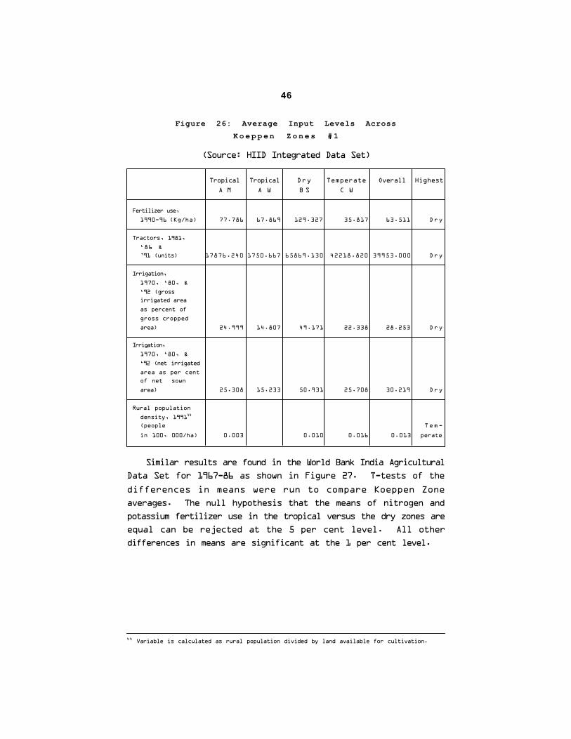
Important determinants of agricultural productivity such as

irrigation, tractors, fertilizer use, and rural literacy are all highest

in the dry zones according to the HIID Integrated Data Set, as

shown in Figure 26. See Appendix A for maps on irrigation

and crop yields.

46

Figure 26: Average Input Levels AcrossK o e p p e n Z o n e s # 1

(Source: HIID Integrated Data Set)

Tropical Tropical Dry Temperate Overall Highest

A M A W B S C W

Fertilizer use,

1990-96 (Kg/ha) 77.786 67.869 129.327 35.817 63.511 Dry

Tractors, 1981,

‘86 &’91 (units) 17876.240 1750.667 65869.130 42218.820 39953.000 Dry

Irrigation,

1970, ‘80, &

‘92 (grossirrigated area

as percent of

gross cropped

area) 24.999 14.807 49.171 22.338 28.253 Dry

Irrigation,

1970, ‘80, &

‘92 (net irrigated

area as per centof net sown

area) 25.308 15.233 50.931 25.708 30.219 Dry

Rural population

density, 199144

(people Tem-

in 100, 000/ha) 0.003 0.010 0.016 0.013 perate

Similar results are found in the World Bank India Agricultural

Data Set for 1967-86 as shown in Figure 27. T-tests of the

differences in means were run to compare Koeppen Zone

averages. The null hypothesis that the means of nitrogen and

potassium fertilizer use in the tropical versus the dry zones are

equal can be rejected at the 5 per cent level. All other

differences in means are significant at the 1 per cent level.

44 Variable is calculated as rural population divided by land available for cultivation.

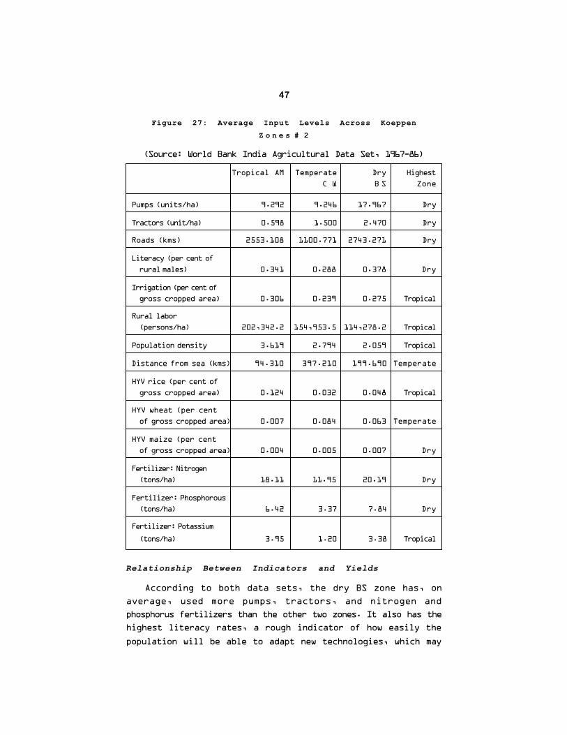
47

Figure 27: Average Input Levels Across KoeppenZ o n e s # 2

(Source: World Bank India Agricultural Data Set, 1967-86)

Tropical AM Temperate Dry HighestC W B S Zone

Pumps (units/ha) 9.292 9.246 17.967 Dry

Tractors (unit/ha) 0.598 1.500 2.470 Dry

Roads (kms) 2553.108 1100.771 2743.271 Dry

Literacy (per cent ofrural males) 0.341 0.288 0.378 Dry

Irrigation (per cent ofgross cropped area) 0.306 0.239 0.275 Tropical

Rural labor(persons/ha) 202,342.2 154,953.5 114,278.2 Tropical

Population density 3.619 2.794 2.059 Tropical

Distance from sea (kms) 94.310 397.210 199.690 Temperate

HYV rice (per cent ofgross cropped area) 0.124 0.032 0.048 Tropical

HYV wheat (per centof gross cropped area) 0.007 0.084 0.063 Temperate

HYV maize (per centof gross cropped area) 0.004 0.005 0.007 Dry

Fertilizer: Nitrogen(tons/ha) 18.11 11.95 20.19 Dry

Fertilizer: Phosphorous(tons/ha) 6.42 3.37 7.84 Dry

Fertilizer: Potassium

(tons/ha) 3.95 1.20 3.38 Tropical

Relationship Between Indicators and Yields

According to both data sets, the dry BS zone has, on

average, used more pumps, tractors, and nitrogen and

phosphorus fertilizers than the other two zones. It also has the

highest literacy rates, a rough indicator of how easily the

population will be able to adapt new technologies, which may

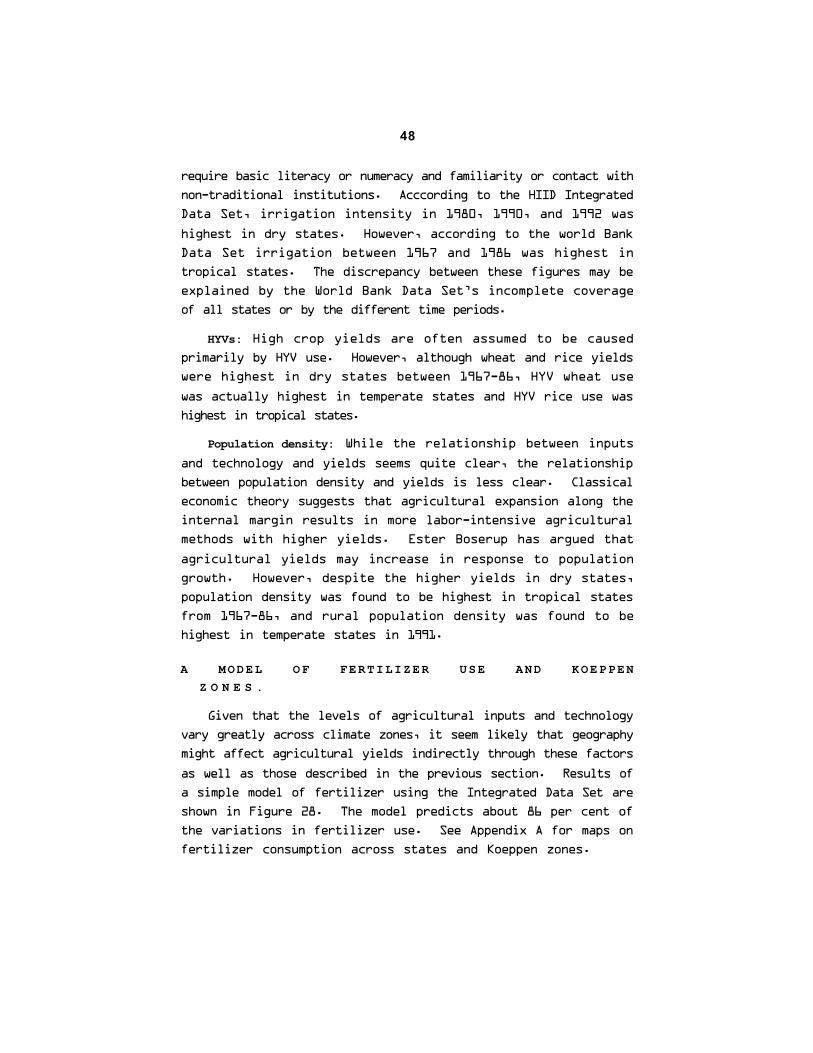
48

require basic literacy or numeracy and familiarity or contact with

non-traditional institutions. Acccording to the HIID Integrated

Data Set, irrigation intensity in 1980, 1990, and 1992 was

highest in dry states. However, according to the world Bank

Data Set irrigation between 1967 and 1986 was highest in

tropical states. The discrepancy between these figures may be

explained by the World Bank Data Set’s incomplete coverage

of all states or by the different time periods.

HYVs: High crop yields are often assumed to be causedprimarily by HYV use. However, although wheat and rice yields

were highest in dry states between 1967-86, HYV wheat use

was actually highest in temperate states and HYV rice use was

highest in tropical states.

Population density: While the relationship between inputs

and technology and yields seems quite clear, the relationship

between population density and yields is less clear. Classical

economic theory suggests that agricultural expansion along the

internal margin results in more labor-intensive agricultural

methods with higher yields. Ester Boserup has argued that

agricultural yields may increase in response to population

growth. However, despite the higher yields in dry states,

population density was found to be highest in tropical states

from 1967-86, and rural population density was found to be

highest in temperate states in 1991.

A MODEL OF FERTILIZER USE AND KOEPPENZ O N E S .

Given that the levels of agricultural inputs and technology

vary greatly across climate zones, it seem likely that geography

might affect agricultural yields indirectly through these factors

as well as those described in the previous section. Results of

a simple model of fertilizer using the Integrated Data Set are

shown in Figure 28. The model predicts about 86 per cent of

the variations in fertilizer use. See Appendix A for maps on

fertilizer consumption across states and Koeppen zones.

49

F I G U R E 2 8 : R E G R E S S I O N O F F E R T I L I Z E R U S E 1 9 9 2( K G / H A )

Irrigation, 1992 (net irrigated 1.489**

area as a per cent of net sown area) (0.000)

Lagged NSDP (log of 1980-81 1.083

value in 1980 US $) (0.661)

Tropical AM zone 54.653*

(0.045)

Tropical AW zone 72.650**

(0.010)

Dry BS zone 68.890

(0.066)

Temperate CW zone 4.080

(0.851)

Constant -27.987

(0.205)


R 2 0.864


*=significant at 1% **=significant at 5%.

F-tests on joint significance, shown in figure 29, illustrate

that the differences in all estimates are significant, except for

the difference between the AM and BS zones, both of which

have very large “effects” of fertilizer use. Clearly, the temper-

ate zone has a much lower positive effect on fertilizer use than

do any of the other zones.

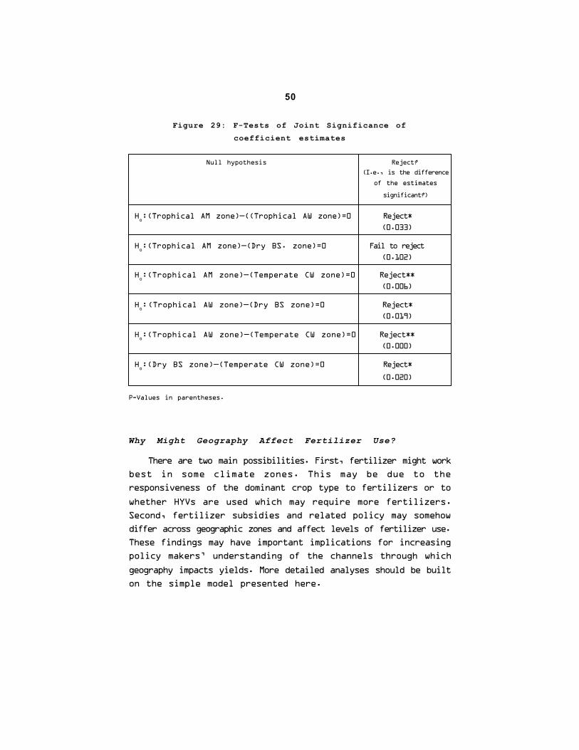
50

Figure 29: F-Tests of Joint Significance ofcoefficient estimates

Null hypothesis Reject?

(I.e., is the difference

of the estimates

significant?)

Ho:(Trophical AM zone)—((Trophical AW zone)=0 Reject*

(0.033)

Ho:(Trophical AM zone)—(Dry BS. zone)=0 Fail to reject

(0.102)

Ho:(Trophical AM zone)—(Temperate CW zone)=0 Reject**

(0.006)

Ho:(Trophical AW zone)—(Dry BS zone)=0 Reject*

(0.019)

Ho:(Trophical AW zone)—(Temperate CW zone)=0 Reject**

(0.000)

Ho:(Dry BS zone)—(Temperate CW zone)=0 Reject*

(0.020)

P-Values in parentheses.

Why Might Geography Affect Fertilizer Use?

There are two main possibilities. First, fertilizer might work

best in some climate zones. This may be due to the

responsiveness of the dominant crop type to fertilizers or to

whether HYVs are used which may require more fertilizers.

Second, fertilizer subsidies and related policy may somehow

differ across geographic zones and affect levels of fertilizer use.

These findings may have important implications for increasing

policy makers’ understanding of the channels through which

geography impacts yields. More detailed analyses should be built

on the simple model presented here.

51

VII. POLICY RECOMMENDATIONS

The following recommendations are options for the Tamil

Nadu Government to incorporate into its existing agricultural

policy. These options have been chosen with budget constrainst

in mind, and are thus least-cost options. Moreover, they do not

require new institutions or capacities. Rather, they involve

strengthening existing institutions.

1. INCLUDE GEOGRAPHIC FACTORS IN ECONOMICANALYSES OF TAMIL NADU’S AGRICULTURE

Cross-national studies show that geography affects growth

through agricultural productivity. This study confirms that

geography impacts state-level variations in agricultural

productivity in India. Variations in precipitation, temperature and

soil quality affect variations in foodgrain yields directly and

possibly, indirectly through the effectiveness of technologies and

inputs. Future analyses of economic growth and agricultural

productivity should, therefore, include geography in order to

fully understand agricultural variations and policy options.

Analysis at the District level

Understanding the geography-related causes of variations in

foodgrain yields within Tamil Nadu can assist the State

Government in determining appropriate investments in

geographically advantaged and disadvantaged districts. The

Government can apply the methods described in this report to

cross district data. Preliminary analyses were made at the district

level for Tamil Nadu using the methods and data described in

this report. The results show that temperature and precipitation

do indeed have significant impacts on rice yields in Tamil Nadu.

(See Appendix D for regression results.)

There have been some attempts to do this using data from

village surveys. A 1992 study of irrigation, HYV rice, and income

distribution in Tamil Nadu by C. Ramasamy,

P. Paramasivam and A. Kandaswamy, for example, finds that

variation in rice yields across villages“strongly suggest that

degree of water control is the decisive factor influencing rice

52

yields”45 The degree of water control, they find, varies across

environments in different administrative districts.46 The Tamil

Nadu Government might build on this village-level data or use

existing cross-district data sources.

Analyses at the Regional and national levels

Geographic analyses on agricultural productivity can also

assist the State Government to better understand its geographic

advantages and disadvantages in relation to other states,

particularly other Southern states. Knowledge of the state’s

disadvantages in agricultural productivity can help it to design

appropriate investments and policies with other states and with

the national government. For example, in 1995, Tamil Nadu’s

agricultural sector suffered from unexpected low levels of water.

Water disputes led to the “non-release of water” by Karnataka

from the Cauvery, which had a large negative effect on Tamil

Nadu’s agricultural productivity.47 A thorough understanding of

geographic disadvantages and their impact on agriculture might

have helped the State Government push for appropriate policies

in advance and thus prevent such situations.

2.EVALUATE THE EFFECTS OF TAMIL NADU’SAGRICULTURAL INPUT POLICIES ON DIFFERENTAGRO-CLIMATIC PRODUCTION ENVIRONMENTS

ACROSS DISTRICTS

This study finds significant variations in input levels across

koeppen Zones in India. Similarly, Ramasamy,. Paramasivam

and Kandaswamy’s study shows differences in input levels across

agro-climatic zones within Tamil Nadu.48 Input policies can

greatly affect such geographic variations in input use. Thus

evaluations on input policies should include separate and com-

plete analyses for both favourable and unfavourable agro-climatic

environments.

45 Ramasamy, C.P. Paramasivam, and A. Kandaswamy. “Irrigation Quality, Modern Variety

Adoption, and Income Distribution: The Case of Tamil Nadu In India,” in Modern rice

Technology and Income Distribution in Asia eds., David, Cristina and Keijiro Otsuka

(Boulder & London: Lynne rienner Publishers, 1994), 331.

46 Ibid, 325-32647 Government of Tamil Nadu, Tamil Nadu-An Economic Appraisal (Chennai: Government

of Tamil Nadu, 1996).

48 Ramasamy, 329.

53

Both Tamil Nadu and the national government have

recognized the importance of agricultural inputs to yields. In

particular, government policies have attempted to increase

agricultural input levels through subsidies for fertilizer, irrigation,

water and power, as well as through infrastructure projects.

These policies are complex and spark considerable debate. This

analysis does not attempt to take sides on this debate.

Rather, this analysis suggests a new way to evaluate these

policies to include the impact of geography on input use. If input

levels vary significantly across environments, and input levels

are linked both to agricultural productivity and to income,

unfavourable environments can be targeted to meet the goals

of increasing growth and reducing poverty. Favourable

environments may also be targeted to ensure the highest returns

on input investments. Agricultural input policies should then be

judged successful if they increase input levels and yields in

unfavourable environments, as well as in favourable ones.

The first step to this process, as described in

Recommendation#1, will be to identify which areas in Tamil

Nadu have geographic advantages and disadvantages for

agriculture. Then the Government can determine the true effect

of input policies in various regions.

3. ENCOURAGE RESEARCH ON NEWTECHNOLOGIES ADAPTED TO TAMIL NADU’S

G E O G R A P H Y

This study finds that geographic variables are important

determinants of yields. The State Government of Tamil Nadu

cannot, of course, change the state’s geographic profile. It can,

however, increase yields by encouraging public, private, and

international research on agricultural technologies that are well-

suited to the state’s geography.

India has one of the largest publicly funded agricultural

research systems in the world. According to a recent study by

Robert Evenson, Carl Pray and Mark Rosegrant, public

agricultural research accounted for nearly 40 per cent of total

54

factor productivity growth in Indian agriculture between 1956

and 1987.49 Since the mid-1970s however, public research

growth has experienced regional variation. Much of the national-

level research funding from the Indian Council of Agricultural

Research (ICAR) is channeled through state governments and

state agricultural universities. Although universities cover all

regions in India, agricultural research in the North enjoys the

most resources in terms of levels and as a per cent of agricultural

GDP. This can largely be attributed to the strong state support

for research in the North.50

The Tamil Nadu Government should encourage more

agricultural research for the South. Increased research in the

South can help ensure research on technology that is fit for the

South’s geographic profile. Currently, Tamil Nadu has the lowest

levels of expenditure on agricultural research of the southern

states, although its expenditure as a percentage of agricultural

GDP is second only to Kerala.

To help promote agricultural research for the South’s

geography, the State Government can:

* Push for more ICAR resources toward the South’s state

agricultural universities.

* Expand existing public programs, such as the Rice-Wheat Consortium, a program of the CGIAR, to movebeyond the Indo-Gangetic Plain to also include tropical

regions.

* Increase ties with existing International Institutions, such

as International Crops Research Institute for the Semi-

Arid Tropics and the International Rice Research Institute

(IRRI), based in Andhra Pradesh.

* Encourage private sector research. Private research has

increased dramatically since the 1960s, it is highly

efficient, and it imposes no burden on the public budget.

49 Evenson, Robert, Carl Pray and Mark Rosegrant, “Agricultural Research and Productivity

Growth in India” (Washington, DC: International Food Policy Research Institute, 1999).

1-5.

50 Ibid, 5-26.

55

* Increase ties with the national Agricultural Research

System (NARS). NARS connects all ICAR institutes, state

agricultural universities, and zonal research centres es-

tablished under the National Agricultural Research

Project (NARP).

* Increase ties with central government departments that

provide some funding for agricultural research, such as

the Ministry of Commerce or the Ministry of Science

and Technology.

The state might also refer to existing analyses of how to

prioritize research to correct for Tamil Nadu’s geographic

disadvantages. A possible starting point is the comprehensive

analysis of rice research priorities in Southern India done by

C.Ramasamy, T.R. Shanmugham, and D. Suresh of the Tamil

Nadu Agricultural University. The study first identified “techni-

cal constraints” to yields, including insects and pests; diseases;

soils/agronomy; genetic/physiological; and climatic and environ-

mental factors. It then estimated the severity of specific con-

straints and potential benefits to “solving” them against the

research costs of “solving” them. according to this study, Tamil

Nadu’s top five yield constraints are leaf folder, ear head bug,

fertilizer imbalance, rice blast, and water management51.

4. SUPPORT THE ADOPTION OF EXISTING

TECHNOLOGIES SUITED TO TAMIL NADU’SG E O G R A P H Y

In addition to promoting new technology through increased

research, the State Government can help increase yields by

promoting the adoption of existing technology that is well suited

to Tamil Nadu’s geography. To this end, the Tamil Nadu

Government can review and evaluate existing technologies and

their varying success in different geographic zones. Through the

use of demonstration sites at the district level, the Government

can increase farmers’ awareness of which technologies are most

appropriate for various geographic characteristics. Because HYV

51 Ramasamy, C,. T.R. Shanmugham, and D. Suresh “Constraints to Higher rice Yields in

different Rice Production Environments and prioritization of Rice Research in Southern

India, “in Rice Research in Asia: Progress and Priorities,

56

success and adoption are so closely linked with water

availability, the Tamil Nadu Government should continue its

focus on supporting irrigation projects throughout the state.

Further, the government can facilitate the adoption HYVs

that are fit for the geographic conditions in Tamil Nadu simply

by urging the national government to make them available on

the market for purchase by farmers. Currently, India’s seed

industry is highly regulated and many HYVs available in other

tropical regions are not available in Tamil Nadu or in India.

The Indian government expends significant resources in testing

HYVs to find the best ones to release in the market, but this

process can be time consuming. For example, the ICAR’s Rice

Improvement Programme took from 1991-1995 to release just

four high yield rice varieties for use in Karnataka, Tamil Nadu,

and Andhra Pradesh52. The Tamil Nadu Government should

support efforts to hasten the government’s release of HYVs that

are suited to use in tropical regions.

5. ADDRESS CONCERNS OF AGRICULTURAL RISKCAUSED BY TAMIL NADU’S CLIMATE

This study clearly illustrates that rainfall and temperature

play important roles in agricultural yields. Moreover, volatile

rainfall and temperature seem to have negative impacts on yields

in India. The “Production risk” due to weather is peculiar to

the agricultural sector as compared to industry53. Uncertainty

from volatile weather can hurt poor farmers who lack savings

and credit to protect them in bad seasons. In addition, uncer-

tainty can lead farmers to give up higher yields in return for

certainty, and can thus slow growth in the agricultural sector.

To reduce risk, for example, many farmers plant two different

crops with different rainfall needs, thereby reducing overall yields

and profits. In addition, Many farmers opt for traditional seeds

over HYVs, because HYVs have higher variability in yields.

The State Government should help address farmers’ concerns

eds. Evenson, R.E. and R.W. Herdt with M. Hossain (CAB International, 1996) 146-160.52 Food and Agriculture Organisation, “Support to Indias, Rice improvement Programme —

IND/91/008,”http://www.fao.org/ag/agp/agpc/promo/india.htm. The Programme was initi-ated in 1989 and approved for funding by the UNDP/FAO in1991.

53 Mishra, Pramod K., Agricultural risk, Insurance and Income (Aldershot: Avebury, 1996),

11.

57

of agricultural risk caused by climate to maximize farmers’ efforts

to attain higher yields.

Two Options to Reduce Production Risks

First, the Government can reduce the costs of uncertainty

about weather by increasing information. As the Food and

Agriculture organization notes, “Farmers in developing and tropi-

cal countries could benefit enormously from access to inter-

preted agrometeorological data and improved seasonal fore-

casts. An accurate idea of the rainfall already in the soil, as

well as that confidently predicted, would allow them to plant

the right crop at the right time”.54 In Mali, for example, under

the AGRHYMET program, extension workers have used accu-

rate weather information to advise farmers about what to plan

and when. An International Workshop on Agrometeorology in

the Twenty-First Century, in February 1991, identified related

priority areas that are relevant to Tamil Nadu. These include

the support of networks of climatological stations and the pro-

vision of “training in agrometeorology to all agriculture profes-

sionals with secondary school or higher education”55.

Second, the State Government should build on existing

institutions to improve access to insurance and credit to farm-

ers. Tamil Nadu currently has the largest credit/deposit ratio in

the country. The Government of Tamil Nadu can work through

the Comprehensive Crop Insurance Scheme (CCIS), which the

Indian national government introduced in 1985-86 and oper-

ates with the assistance of state governments through the

General Insurance Corporation of India. A significant limitation

of the CCIS for Tamil Nadu is its selective coverage of crops,

not including Tamil Nadu’s principal crop, rice. Another draw-

back is that state supported insurance and credit may pose a

significant drain on the public budget.56

54 Food and Agriculture Organisation, “Weather-wise farmers could improve yields,” March

30, 1999, http://www.fao.org/news/1999/990307-ehtm, 2. For further information, con-

tact Rene.Gommes @fao.org.

55 LIbid, 2.

56 For further information on the CCIS, see Mishra, Pramod K. Agricultural Risk, Insur-

ance and Income: A study of the Impact and Design of India’s Comprehensive CropInsurance Scheme (Aldershot: Avebury, 1996).

58

The State Government can also increase ties with the growing

body of private and non-governmental organizations (NGOs)

involved in credit and insurance initiatives. The private sector

has access to efficient management techniques, experience in

lending, and substantial resources. The NGOs have access to

large community groups, experience with capacity building, and

local training initiatives that maximize the use of credit services.

The partnership between the private and NGO groups is grow-

ing rapidly across the world. The State Government should make

concerted efforts to remain a key actor in this partnership.

6. CONTINUE INVESTMENTS IN TAMIL NADU’SMANUFACTURING AND TRADE SECTORS

This report argues that geography has significant effects on

agricultural productivity, even holding constant income and other

factors of production. Technology and higher input levels may

have only limited impact on mitigating geographic effects on

agricultural yields. Tamil Nadu, along with other tropical AM

and AW states, is at a slight disadvantage in agricultural

productivity compared to dry BS states. In the long run, Tamil

Nadu may naturally shift away from agriculture to other, more

profitable sectors of the economy, like manufacturing. Tamil

Nadu already appears to be making this transition. The State

Government should continue to support it through investments

in industry and trade.

At present, however, the Tamil Nadu Government is well

advised to continue efforts toward increased understanding of

agriculture and well-targeted investments. The agricultural sector

has significant effects on rural poverty and on state and national

food security. Growth in agriculture provides a firm basis for

both economic growth and poverty alleviation.

59

B I B L I O G R A P H Y

Athreya, Venkatesh and Sheela Rani Chunkath. “Gender

and Infant Survival in Rural Tamil Nadu: Situation and

Strategy.” Economic and Political Weekly (October 3,1998): 2588-2594.

Bajpai, Nirupam and Jeffrey D. Sachs. “Strengthening

India’s Strategy for Economic Growth.” Harvard Institute

for International Development (July 1998).

Development Discussion Paper No. 641.

Bhalla, G.S. and Peter Hazell, “Foodgrains Demand in

India to 2020: A Preliminary Exercise.” Economic and

Political Weekly (December 27, 1997): A150-A154.

Bhalla, G.S. and Gurmail Singh. “Recent Developments in

Indian Agriculture: A State Level Analysis”. Economic

and Political Weekly (March 29, 1997): A2-A18.

Bloom, David E. and Jeffrey D. Sachs. “Geography,

Demography, and Economic Growth in Africa.” HarvardInstitute for International Development, September1998. First draft.

Centre for Monitoring Indian Economy, Agriculture, August1997 Mumbai: CMIE, 1997.

Centre for Monitoring Indian Economy. Agriculture,September 1998. Mumbai: CMIE, 1998.

Chand, Ramesh and T. Haque. “Sustainability of Rice-

Wheat Crop system in Indo-Gangetic Region.” Economicand Political Weekly (March 29, 1997): A26—A30.

Chattopadhyay, Manabendu and Atanu Sengupta. “Farm

Size and Productivity: A New Look at the Old Debate.”

Economic and Political Weekly (December 27, 1997):A172-A175.

Chopra R.N. Evolution of Food Policy in India, New Delhi:Macmillan India Ltd., 1981.

Dagli, Vadilal, ed. A Regional Profile of Indian Agriculture,Bombay: Vora & Co., Publishers, 1974.

60

Datt, Gaurav and Martin Ravallion. “Why have some

Indian states done better than others at reducing rural

poverty?” Washington, DC: World Bank, Policy Research

Department, January 21, 1997, Photocopied.

David, Cristina C. and Keijiro Otsuka. Modern Rice Tech-nology and Income Distribution in Asia. Boulder and

London: Lynne Rienner Publishers, 1994.

Desai, Bhupat M. and N.V. Namboodiri. “Determinants of

Total Factor Productivity in Indian Agriculture.” Eco-

nomic and Political Weekly (December 27, 1997) A165-A171.

Desai, Bhupat M. and N.V. Namboodiri. “Developing Ag-

riculture in Gujarat: A Strategic Perspective for Ninth

Plan.” Economic and Political Weekly (March 29, 1997):

A31-A40.

Datt, Gaurav and Martin Ravallion, “Farm Productivity and

Rural Poverty in India.” The Journal of DevelopmentStudies 34.4. (April 1988): 62-85.

Dev. S. Mahendra, “Summaries of Group Discussion:

Regional Variations in Agricultural Performance in the

Last Two Decades.” Indian Journal of AgriculturalEconomics 53.1 (January-March 1998): 15-18.

Dhawan, B.D. “Production Benefits from Large-Scale Canal

Irrigation.” Economic and Political Weekly (December

27, 1997): A177-A181.

Dhawan, B.D. and S.S. Yadav. “Public Investment in Indian

Agriculture: Trends and Determinants.” Economic and

Political Weekly (April 5, 1997): 710-714.

Dinar, Ariel, Robert Mendelsohn, Robert Evenson, Jyoti

Parikh, Apurva Sanghi, Kavi Kumar, James McKinsey,

and Stephen Lonergan. Measuring the Impact of Cli-mate change on Indian Agriculture. Washington, DC:The World Bank, 1998. World Bank Technical paper

No. 402.

61

Dreze, Jean and Amartya Sen. India Economic Developmentand Social Opportunity. Delhi Oxford University Press,1995.

Economist Intelligence Unit. India 1998-99,Country Profile.

http://www.eiu.com.

Evenson, Rob, Pray, Carl and Rosegrant, Mark, “Agricultural

Research and Productivity Growth in India”

(Washington, D.C.: International Food Policy Research

Institute, 1999).

Food and Agriculture Organisation. “Support to India’s Rice

Improvement Programme—IND/91/008.” http://

www.fao.org/ag/agpc/promo/india.htm.

Food and Agriculture Organisation, “Weather-wise farmers

could improve their yields.” FAO News Highlights

(March 30, 1999). http://www.fao.org/news/1999/

990307-e.htm.

Gallup, John Luke. “Agricultural productivity and

Geography.” Harvard Institute for International

Development, January 1998.

Gallup, John Luke and Jeffrey Sachs, with Andrew D.

Mellinger. “Geography and Economic Development.”

Harvard Institute for Internal Development, 1998.

Photocopied.

Gillespie, Stuart and McNeil, Geraldine. Food, Health andSurvival in India and Developing Countries. Oxford

University Press, Delhi, 1992.

Government of India, Ministry of Finance, Economic

Division. Economic Survey 1998-99. New Delhi:

Government of India Press, 1999.

Government of Tamil Nadu, Agriculture Department. TamilNadu Agricultural Policy. November 1995.

Government of Tamil Nadu, Evaluation and Applied

Research Department. Tamil Nadu—An EconomicAppraisal, 1995-96.

62

Kabra, Kamal and Ittyerah, Anil. The Public DistributionSystem in India. Eastern Books, New Delhi, 1992.

Kalirajan, K.P. and R.T. Shand. “Sources of Output Growth

in Indian Agriculture” Indian Journal of AgriculturalEconomics 52 (October-December 1997): 693-706.

Klohn, Wulf E. and Bo G. Appelgren. “Challenges in the

field of water resources management in Agriculture.”

Food and Agriculture Organisation.

http://www.fao.org/WAICENT/FAOINFO/AGRICULT/AGL/

AGLW/webpub/ath-kln/ATH-KLM.htm.

Krugman, Paul.“The Role of Geography in Development.”1999. Photocopied.

Kumar, Praduman, Mark Rosegrant, and Peter Hazell,

“Cereals Prospects in India to 2020: Implications forPolicy.” IFPRI 2020 Vision Brief 23 (June 1995). http://www.cgiar.org/ifprl/2020/briefs/number23.htm.

Madras Institute of Development Studies, Tamil NaduEconomy, Performance and Issues. Oxford and IBH

Publishing Co., New Delhi, 1988.

Mishra, Pramod K. Agricultural Risk, Insurance and Income:

A Study of the Impact and Design of India’s Compre-

hensive Crop Insurance Scheme. Aldershot: Avebury,

1996.

Mishra, S.N. “Agricultural Liberalization and Development

Strategy in Ninth-Plan.” Ecomomic and Political Weekly

(March 29, 1997): A19-A25.

Ministry of Agriculture, Area and Production of Principal

Crops in India. (New Delhi: Ministry of Agriculture,

Volumes 1987-1994).

Ministry of Agriculture, Agricultural Statistics at a Glance.

(New Delhi: Image Print, 1998).

Ministry of Agriculture, Indian Agriculture in Brief, 26thEdition (New Delhi: Government of India Press, 1995).

63

Mukherjee, Amitava. Structural Adjustment Program and

Food Security. Avebury, Aldeshot, 1994.

Mundlak, Yair, Donald Larson, Rita Butzer, “The

Determinants of Agricultural Production: A Cross-

Country Analysis.” March 16, 1997. Photocopied.

Parikh, Kirit S., ed. India Development Report 1997. IndiraGandhi Institute of Development Research. Delhi: Oxford

University Press, 1996.

Perumalsamy, S. Ecomomic Development of Tamil Nadu,S. Chand and Company Ltd. Ramnagar, New Delhi,

1996.

Raj, K.N., Amartya Sen and C.H. Hanumantha Rao, eds.

Studies in Indian Agriculture. Delhi: Oxford UP, 1988.

Ramasamy, C., T.R. Shanmugam, D. Suresh. “Constraints

to Higher Rice Yields in Different Rice Production

Environments and Prioritization of Rice Research in

Southern India.” In Rice Research in Aisa: Progress and

Priorities, eds. R.E. Evenson and R.W. Herdt with M.Hossain, 145-160. CAB International, 1996.

Rao, V.M. “Agricultural Development with a Human Face:

Experiences and Prospects.” Economic and PoliticalWeekly (June 29, 1996): A50-A62.

Rawal, Vikas and Madura Swaminathan, “Changing

Trajectories: Agricultural Growth in West Bengal, 1950

to 1996.” Economic and Political Weekly (October 3,1998): 2595-2602.

Sanderson, Fred and Roy, Shyamal. Food Trends andProspects in India. The Brookings Institution,

Washington, D.C.,1979.

Sanghi, Apurva, K.S. Kavi Kumar and James W. McKinsey,

Jr. “India Agriculture and Climate Data Set.” The world

Bank. http://www-esd.worldBank/org/indian/

database.html.

64

Sawant, S.D. “Performance of India Agriculture with Special

Reference to Regional Variations.” Indian Journal OfAgricultural Economics 52 (July-September 1997):

354-373.

Scandizzo, Pasquale and Swamy, Gurushri, “Benefits and

Costs of Food Distribution Policies; The India Case.”

World Bank Staff Working Papers, No.509. WashingtonD.C., The World Bank, 1982.

Singh, I.J., K.N. Rai and J.C. Karwasra. “Regional

Variations in Agricultural Performance in India.” Indian

Journal of Agricultural Economics 52 (July - September

1997): 374-386.

Timmer, C. Peter and Falcon, Walter and Pearson, Scott.

Food Policy Analysis. John’s Hopkins University Press,

Baltimore, 1983.

Varma, Ram K. Economic Geography and AgriculturalGrowth. Jaipur; Printwell, 1996.

Winters, Paul, et al. “The Role of Agriculture in Economic

Development: Visible and Invisible Surplus Transfers.”

The Journal of Development Studies 34.5 (June 1998):71-97.

World Bank, Operations Evaluation Development. “The

Seed Industry in South Asia.” OED Precis 112 (May1996). http://www.worldbank.org/html/oed/pr112.htm.

65

A P P E N D I C E S

A. Maps of Regional Foodgrain Trends and Inputs

B. Stete Geography and Foodgrain Yields

C. Regression Results for Model#2

D. Tamil Nadu Regression

66

APPENDIX A

MAPS OF REGIONAL FOODGRAIN TRENDSAND INPUTS

This appendix corresponds with Section III: Regional

Foodgrain Trends; Section V: A Model of Geography and

Foodgrain Yields; and Section VI; Additional Differences Across

Koeppen Zones.

It includes maps for total foodgrains, rice, wheat, and maize

yield and production; net sown area, irrigation and fertilizer

use.

Rice:

* Rice Yield 1980

* Rice Yield 1992

* Rice Production 1980

* Rice Production 1996

Wheat:

* Wheat Yield 1980

* Wheat Yield 1992

* Wheat Production 1980

* Wheat Production 1992

Maize:

* Maize Yield 1980

* Maize Yield 1992

Total Foodgrain:

* Foodgrain Yield 1980

* Foodgrain Yield 1996

* Net Sown Area 1980

* Net Sown Area 1992

67

Irrigation:

* Rice Yield and Irrigation 1980

* Rice Yield and Irrigation 1992

* Wheat Yield and Irrigation 1980

* Wheat Yield and Irrigation 1992

* Maize Yield and Irrigation 1980

* Maize Yield and Irrigation 1992

Fertilizer:

* Fertilizer Consumption 1992

* Fertilizer Consumption 1996

* Koeppen Zone and Fertilizer Consumption 1992

68

APPENDIX B

STATE GEOGRAPHY AND FOODGRAIN YIELDS

This appendix corresponds with Section IV: State Geogra-

phy and Foodgrain Yields. It includes the following tables,

charts and maps for 5 geographic variables:

Variable 1: Koeppen Zones

* Guide to Koeppen Zone Classification

* Percent of State Land in Each Koeppen Zone

* States Listed by Koeppen Zone

* Map of Koeppen Zones

* Chart of Koeppen Zones and Yields

Variable 2: Average Precipitation

* Chart of Average Precipitation and Yields, with classifica-

tion of States in Each Division

Variable 3: Elevation

* Chart of Elevation and Yields, with Classification of States

in Each Division

Variable 4: Distance to the Nearest Navigable River

* Chart of distance and Yields, with Classification of States

in Each Division

Variable 5: Soil Suitability Index

* Chart of Soil Suitability Index and Yields, with Classifica-

tion of States in Each Division.

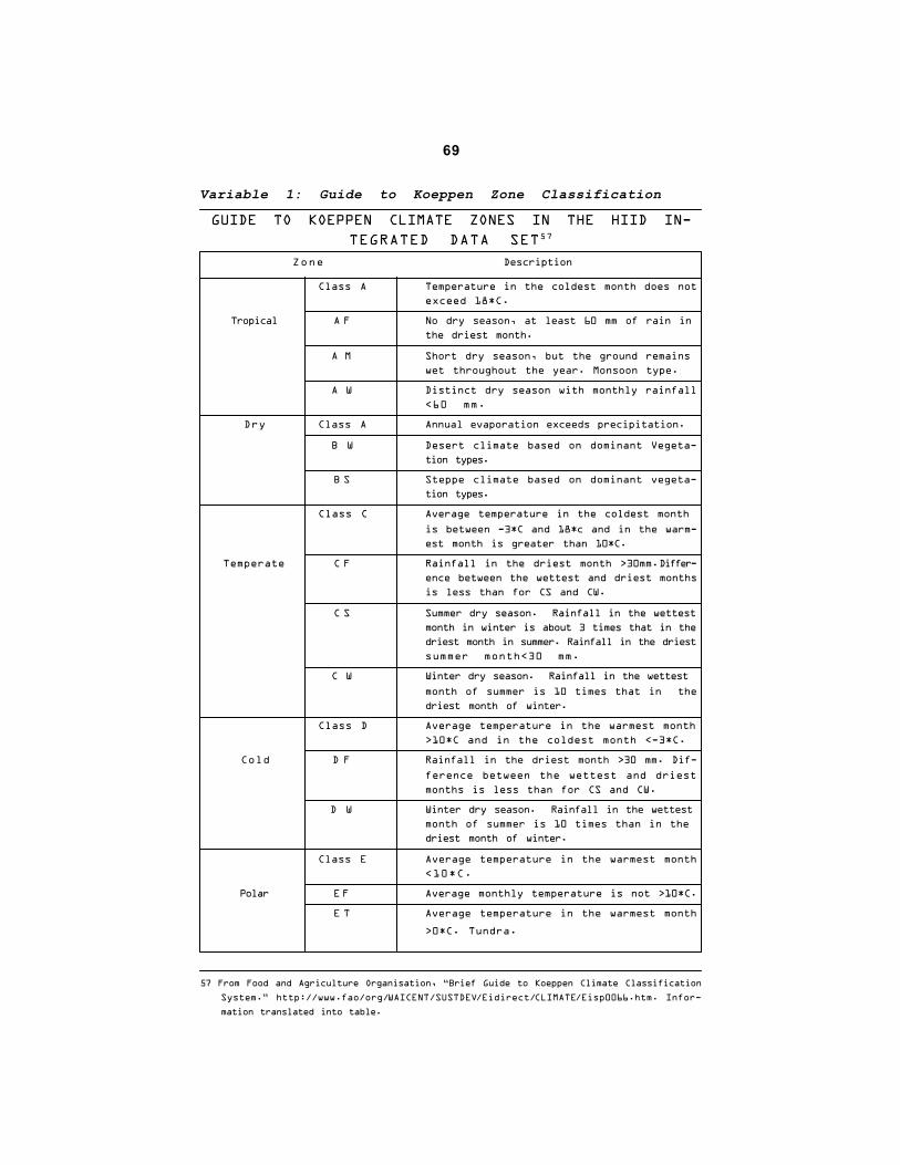
69

57 From Food and Agriculture Organisation, “Brief Guide to Koeppen Climate Classification

System.” http://www.fao/org/WAICENT/SUSTDEV/Eidirect/CLIMATE/Eisp0066.htm. Infor-

mation translated into table.

Variable 1: Guide to Koeppen Zone Classification

GUIDE TO KOEPPEN CLIMATE ZONES IN THE HIID IN-TEGRATED DATA SET57

Zone Description

Class A Temperature in the coldest month does notexceed 18*C.

Tropical A F No dry season, at least 60 mm of rain inthe driest month.

A M Short dry season, but the ground remainswet throughout the year. Monsoon type.

A W Distinct dry season with monthly rainfall<60 mm.

Dry Class A Annual evaporation exceeds precipitation.

B W Desert climate based on dominant Vegeta-tion types.

B S Steppe climate based on dominant vegeta-tion types.

Class C Average temperature in the coldest month

is between -3*C and 18*c and in the warm-est month is greater than 10*C.

Temperate C F Rainfall in the driest month >30mm.Differ-ence between the wettest and driest monthsis less than for CS and CW.

C S Summer dry season. Rainfall in the wettestmonth in winter is about 3 times that in thedriest month in summer. Rainfall in the driestsummer month<30 mm.

C W Winter dry season. Rainfall in the wettest

month of summer is 10 times that in thedriest month of winter.

Class D Average temperature in the warmest month>10*C and in the coldest month <-3*C.

Cold D F Rainfall in the driest month >30 mm. Dif-

ference between the wettest and driestmonths is less than for CS and CW.

D W Winter dry season. Rainfall in the wettestmonth of summer is 10 times than in thedriest month of winter.

Class E Average temperature in the warmest month<10*C.

Polar E F Average monthly temperature is not >10*C.

E T Average temperature in the warmest month

>0*C. Tundra.

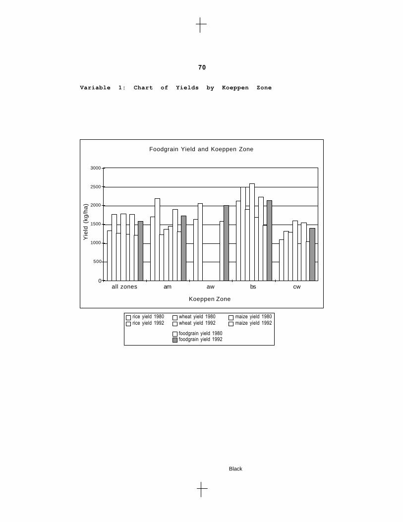
Variable 1: Chart of Yields by Koeppen Zone

70

Yellow Cyan Magenta Black

0

Foodgrain Yield and Koeppen Zone

500

1000

1500

2000

2500

3000

Yie

ld (

kg/h

a)

Koeppen Zone

all zones am aw bs cw

rice yield 1980 wheat yield 1980 maize yield 1980 rice yield 1992 wheat yield 1992 maize yield 1992

foodgrain yield 1980 foodgrain yield 1992

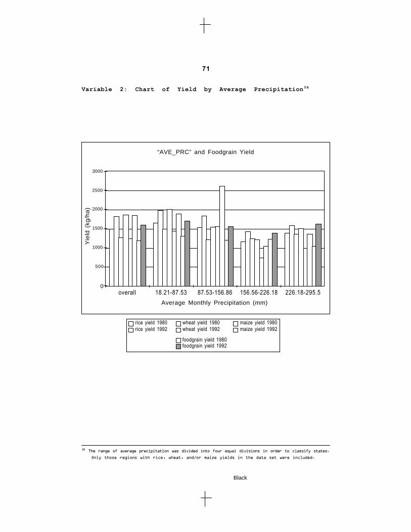
Variable 2: Chart of Yield by Average Precipitation58

58 The range of average precipitation was divided into four equal divisions in order to classify states.

Only those regions with rice, wheat, and/or maize yields in the data set were included.

71

0

“AVE_PRC” and Foodgrain Yield

500

1000

1500

2000

2500

3000

Yie

ld (

kg/h

a)

Average Monthly Precipitation (mm)

overall 18.21-87.53 87.53-156.86 156.56-226.18 226.18-295.5




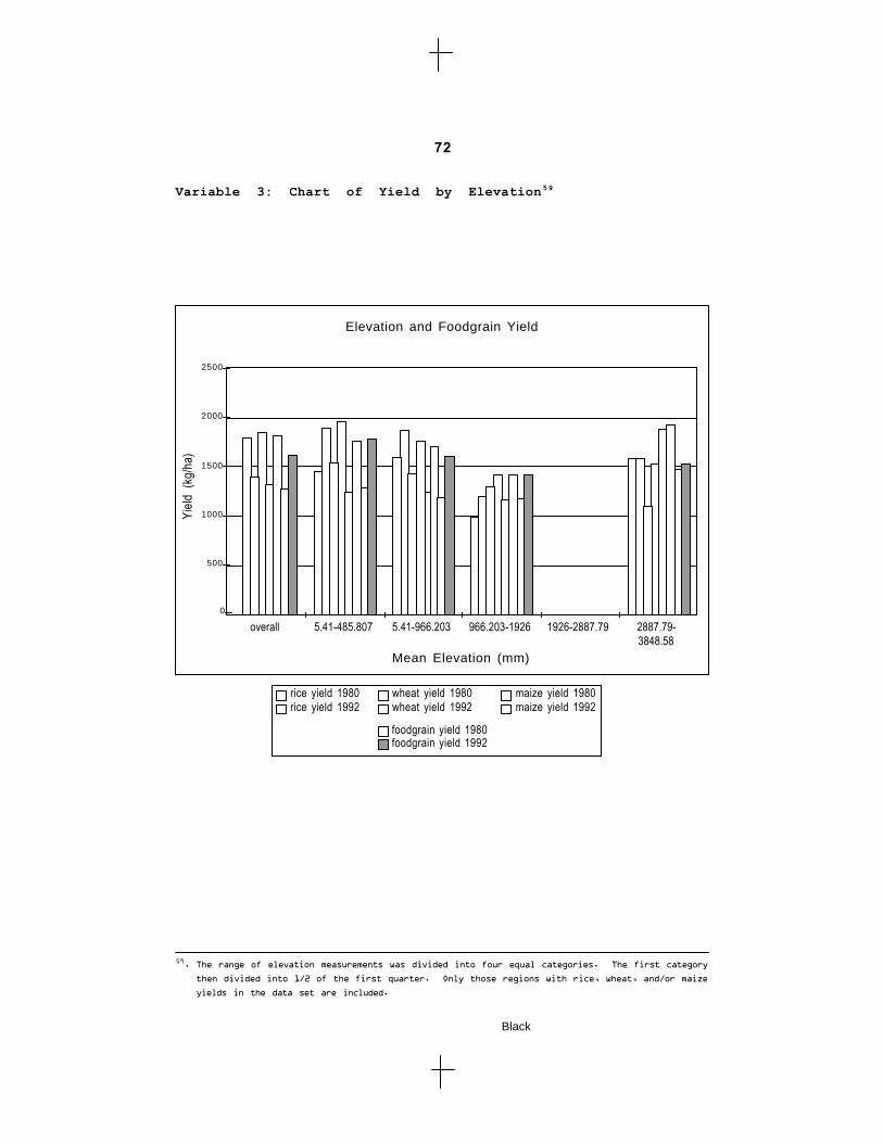
500

1000

1500

2000

2500

72


Variable 3: Chart of Yield by Elevation59

59. The range of elevation measurements was divided into four equal categories. The first category

then divided into 1/2 of the first quarter. Only those regions with rice, wheat, and/or maize

yields in the data set are included.

Elevation and Foodgrain Yield

Yield

(kg

/ha)

Mean Elevation (mm)

overall 5.41-485.807 5.41-966.203 966.203-1926 1926-2887.79 2887.79-3848.58



0

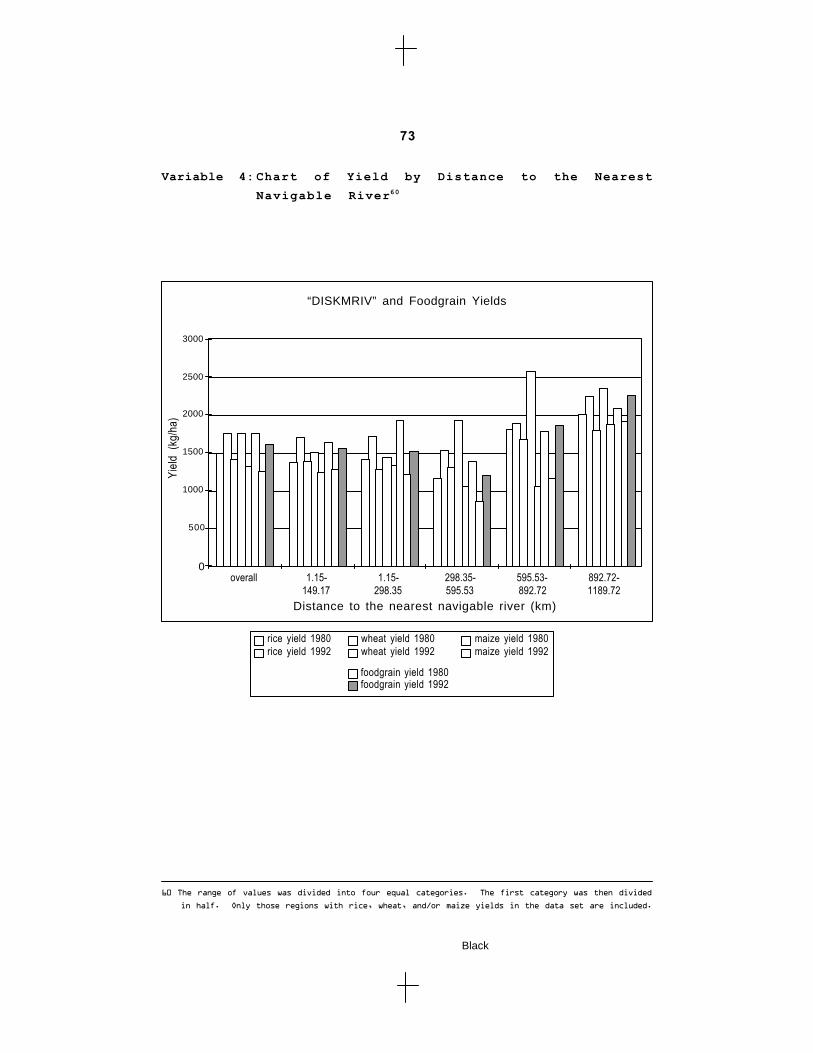
500

1000

1500

2000

2500

3000

73


60 The range of values was divided into four equal categories. The first category was then divided

in half. Only those regions with rice, wheat, and/or maize yields in the data set are included.

Variable 4: Chart of Yield by Distance to the NearestNavigable River60



0

“DISKMRIV” and Foodgrain Yields

Yield

(kg

/ha)

Distance to the nearest navigable river (km)

overall 1.15- 1.15- 298.35- 595.53- 892.72-149.17 298.35 595.53 892.72 1189.72

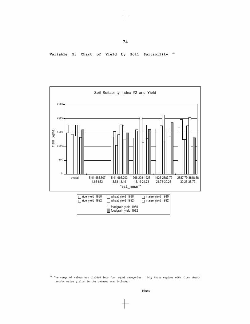
74


Variable 5: Chart of Yield by Soil Suitability 61

61 The range of values was divided into four equal categories. Only those regions with rice, wheat,

and/or maize yields in the dataset are included.

500

1000

1500

2000

2500

Soil Suitability Index #2 and Yield

Yield

(kg

/ha)

“ss2_mean”

overall 5.41-485.807 5.41-966.203 966.203-1926 1926-2887.794.66-853 8.53-13.19 13.19-21.73 21.73-30.26



2887.79-3848.5830.26-38.79

0

Documents

GEOGRAPHY AND AGRICULTURAL PRODUCTIVITY … · Why Study Geography and Agriculture? 2 Why Does this Analysis Focus on Foodgrains?4 Other Analysis of Agricultural Productivity in India6