GEODETIC OBSERVATIONS OF THE OCEAN SURFACE TOPOGRAPHY, GEOID,

CURRENTS, AND CHANGES IN OCEAN MASS AND VOLUME

C.K. Shum(1)

, Hans-Peter Plag(2)

, Jens Schröter(3)

, Victor Zlotnicki(4)

, Peter Bender(5)

, Alexander Braun(6)

,

Anny Cazenave(7)

, Don Chamber(8)

, Jianbin Duan(1)

, William Emery(9)

, Georgia Fotopoulos(6)

,

Viktor Gouretski(10)

, Richard Gross(4)

, Thomas Gruber(11)

, Junyi Guo(1)

, Guoqi Han(12)

, Chris Hughes(13)

,

Masayoshi Ishii(14)

, Steven Jayne(15)

, Johnny Johannessen(16)

, Per Knudsen(17), Chung-Yen Kuo

(18),

Eric Leuliette(19)

, Sydney Levitus(20)

, Nikolai Maximenko(21)

, Laury Miller(19)

, James Morison(22)

,

Harunur Rashid(23)

, John Ries(24)

, Markus Rothache(25)

, Reiner Rummel(11)

, Kazuo Shibuya(26)

,

Michael Sideris(27)

, Y. Tony Song(4)

, Detlef Stammer(28)

, Maik Thomas(29)

, Josh Willis(4)

,

Philip Woodworth(13)

(1) Division of Geodetic Science, School of Earth Sciences, Ohio State University, 275 Mendenhall, 125 S. Oval Mall

43210 Columbus USA, Email: ckshum@osu.edu; duan.29@osu.edu; guo.81@osu.edu (2)

Nevada Bureau of Mines & Geology & Seismology Lab., University of Nevada, Mail Stop 178,

1664 N. Virginia Street, 89557 Reno Nevada 89557, USA, Email: hpplag@unr.edu (3)

Alfred-Wegener-Institute for Polar & Marine Research, Postfach 120161, D-27515 Bremerhaven, Germany,

Email: Jens.Schroeter@awi.de (4)

Jet Propulsion Laboratory, California Institute of Technology, 4800 Oak Grove Dr., Pasadena, CA 91109 USA,

Email: Victor.Zlotnicki@jpl.nasa.gov; Tony.Song@jpl.nasa.gov; richard.gross@jpl.nasa.gov;

joshua.k.willis@jpl.nasa.gov (5)

Joint Institute for Laboratory Astrophysics, University of Colorado & NIST (National Institute of Standards and

Technology), 440 University of Colorado, Boulder, CO 80309-5004 USA, Email: pbender@jila.colorado.edu (6)

Department of Geosciences, University of Texas at Dallas, FO 21, 800 West Campbell Road, Richardson,

TX 75080-302 USA, Email: braun@utdallas.edu; foto@utdallas.edu (7)

LEGOS (Laboratoire d'Études en Géophysique et Océanographie), Centre National d'Études Spatiales,

18, av. Edouard Belin, 31401 Toulouse Cedex 9 France, Email: anny.cazenave@cnes.fr (8)

College of Marine Science, University of South Florida, 140 7th Ave S, St. Petersburg, FL 33701 USA,

Email: dchambers@marine.usf.edu (9)

Colorado Center for Astrodynamics Research, University of Colorado, ECNT 320, 431 UCB, University of

Colorado, Boulder, CO 80309-0431 USA, Email: emery@colorado.edu (10)

KlimaCampus Universität Hamburg, Bundesstr. 53, 20146 Hamburg, Germany, Email: viktor.gouretski@zmaw.de;

detlef.stammer@zmaw.de (11)

Institute of Astronomy & Physical Geodesy, Technische Universität Muenchen, Arcisstraße 21. D-80333 München.

Germany, Email: thomas.gruber@bv.tum.de; rummel@bv.tu-muenchen.de (12)

Fisheries and Oceans Canada, Northwest Atlantic Fisheries Centre, P.O. Box 5667. St. John's NL A1C 5X1 Canada,

Email: HanG@dfo-mpo.gc.ca (13)

Proudman Oceanographic Laboratory, 6 Brownlow St, Liverpool, Merseyside L3 5DA, United Kingdom,

Email: cwh@pol.ac.uk; plw@pol.ac.uk (14)

Frontier Research Center for Global Change, 3173-25 Showamachi, Kanazawa-ku, Yokohama City, Kanagawa

236-0001, Japan, Email: ism@jamstec.go.jp (15)

Woods Hole Oceanographic Institution, 266 Woods Hole Road, Woods Hole, MA 02543, USA,

Email: sjayne@whoi.edu (16)

Nansen Environmental and Remote Sensing Centre, Thormøhlensgt. 47, N-5006 Bergen, Norway,

Email: johnny.johannessen@nersc.no (17)

National Space Institute, Technical University of Denmark, Anker Engelunds Vej 1. Building 101A, 2nd Floor,

2800 Kgs. Lyngby, Denmark, Email: pk@space.dtu.dk (18)

Department of Geomatics, National Cheng Kung University, No. 1, University Road, Tainan 701, Taiwan,

Email: kuo70@mail.ncku.edu.tw (19)

Laboratory for Satellite Altimetry, NOAA (National Oceanic and Atmospheric Administration), Silver Spring MD

20910-3282, USA, Email: Eric.Leuliette@noaa.gov; Laury.Miller@noaa.gov (20)

Ocean Climate Laboratory, National Ocean Data Center, NOAA (National Oceanic and Atmospheric

Administration), 1315 East-West Highway E/OC1 Silver Spring USA, Email: Sydney.Levitus@noaa.gov (21)

International Pacific Research Center, University of Hawaii, 1680 East West Road, Honolulu, Hawaii 96822, USA,

Email: maximenk@hawaii.edu

(22) Polar Science Center, Applied Physics Lab., University of Washington, 1013 NE 40th St, Seattle, WA 98105-6698,

USA, Email: morison@apl.washington.edu

(23) Byrd Polar Research Center, Ohio State University, Enarson Hall 154 W 12th Avenue, Columbus, Ohio 43210 USA,

Email: rashid.29@osu.edu (24)

Center for Space Research, University of Texas at Austin, 3925 West Braker Lane, Suite 200, Austin, Texas

78759-5321 USA, Email: ries@csr.utexas.edu (25)

Institute of Geodesy & Photogrammetry, ETH (Eidgenössische Technische Hochschule) Zurich,

HG F37/38/39/41/43, Rämistrasse 101, 8092 Zurich, Switzerland, Email: markus.rothacher@ethz.ch (26)

CAEM (Commission for Aeronautical Meteorology), National Institute of Polar Research, 10-3, Midoricho,

Tachikawa, Tokyo 190-8518, Japan, Email: shibuya@nipr.ac.jp (27)

Department of Geomatics Engineering, University of Calgary, 2500 University Dr. NW, Calgary, Alberta T2N 1N4

Canada, Email: sideris@ucalgary.ca (28)

Center for Marine and Climate Research, KlimaCampus Universitat Hamburg, Bundesstr. 53, 20146 Hamburg,

Germany, Email: detlef.stammer@zmaw.de (29)

GFZ (German Research Centre for Geosciences/GeoForschungsZentrum), Telegrafenberg, 14473 Potsdam,

Germany, Email: maik.thomas@gfz-potsdam.de

ABSTRACT

The tools of geodesy have the potential to transform the

Ocean Observing System. Geodetic observations are

unique in the way that these methods produce accurate,

quantitative, and integrated observations of gravity,

ocean circulation, sea surface height, ocean bottom

pressure, and mass exchanges among the ocean,

cryosphere, and land. These observations have made

fundamental contributions to the monitoring and

understanding of physical ocean processes. In particular,

geodesy is the fundamental science to enable

determination of an accurate geoid model, allowing

estimate of absolute surface geostrophic currents, which

are necessary to quantify ocean‟s heat transport. The

present geodetic satellites can measure sea level, its

mass component and their changes, both of which are

vital for understanding global climate change.

Continuation of current satellite missions and the

development of new geodetic technologies can be

expected to further support accurate monitoring of the

ocean. The Global Geodetic Observing System (GGOS)

of the International Association of Geodesy (IAG)

provides the means for integrating the geodetic

techniques that monitor the Earth's time-variable surface

geometry (including ocean, hydrologic, land, and ice

surfaces), gravity field, and Earth rotation/orientation

into a consistent system for measuring ocean surface

topography, ocean currents, ocean mass and volume

changes. This system depends on both globally

coordinated ground-based networks of tracking stations

as well as an uninterrupted series of satellite missions.

GGOS works with the Group on Earth Observations

(GEO), the Committee on Earth Observation Satellites

(CEOS) and space agencies to ensure the availability of

the necessary expertise and infrastructure. In this white

paper, we summarize the community consensus of

critical oceanographic observables currently enabled by

geodetic systems, and the requirements to continue such

measurements. Achieving this potential will depend on

merging the remote sensing techniques with in situ

measurements of key variables as an integral part of the

Ocean Observing System.

1. INTRODUCTION

The guiding thesis of this white paper is that the tools of

geodesy have the potential to transform the Ocean

Observing System. Geodetic observations are unique in

the way that they produce accurate, quantitative, and

integrated observations of gravity, ocean circulation, sea

surface height, ocean bottom pressure changes, and

mass exchanges among the ocean, cryosphere,

atmosphere and land. Specifically, we use continuously

operating satellite altimetry and spaceborne gravity

sensors to measure time series of sea surface slope and

ocean bottom pressure variations and thus infer ocean

circulation and mass distribution variations over a broad

continuum of temporal and spatial scales. Achieving

this potential will depend on merging the geodetic

techniques with in situ measurements of key variables

as an integral part of the Ocean Observing System.

The innovative capabilities of geodesy, as exemplified

by the Global Geodetic Observing System (GGOS,

Tab. 1 [46]) of the International Association of Geodesy

(IAG), include the determination of the Earth's mean

and time-dependent geometric shape, gravity field,

rotation/orientation, and terrestrial reference frame.

Combining the geometric methods with global gravity

observables allows for the inference of mass anomalies,

and mass transports within the Earth's system. The

variations in Earth rotation and polar motion reflect both

mass transports in the Earth system and the exchange of

angular momentum among its components. The study

areas of geodesy are therefore highly relevant to ocean

observations, as they directly relate to ocean dynamics,

and changes in ocean mass and sea level [4]. Changes in

mass are directly related to water mass exchanges

among the ocean, cryosphere, and hydrosphere [55].

GGOS provides the global terrestrial reference frame (in

the form of the International Terrestrial Reference

Frame, ITRF 2008 http://itrf.ensg.ign.fr), which is

mandatory for most Earth observations. The accuracy

and long-term stability of ITRF are crucial to many

ocean observations, and in particular, critical to

accurately measuring global sea level rise.

Table 1: The Global Geodetic Observing System (GGOS). VLBI: Very Long Baseline Interferometry; SLR: Satellite

Laser Ranging; LLR: Lunar Laser Ranging; GNSS: Global Navigation Satellite Systems; DORIS: Doppler

Orbitography and Radio positioning Integrated by Satellite; InSAR: Interferometric Synthetic Aperture Radar; IGS:

International GNSS Service; IAS: International Altimetry Service; IVS: International VLBI Service for Geodesy and

Astrometry; ILRS: International Laser Ranging Service; IDS: International DORIS Service; IERS: International Earth

Rotation and Reference Systems Service; IGFS: International Gravity Field Service; GGP: Global Geodynamics

Project; BGI: International Gravimetric Bureau; IGeS: International Geoid Service. Modified from [46, Ch. 2]

The geodetic tools we discuss here relate primarily to

altimetry and gravimetry (components 1 and 3 of

Tab. 1). Satellite radar altimetry is an established

technique for observing ocean surface height (or shape),

its variability, and sea level change. For long-term

ocean and climate studies (e.g. sea level rise), a series of

TOPEX (Topography Experiment)/Jason-class repeat

track radar altimetry satellite missions is a critical

requirement. Data from non-repeat satellite altimetry

missions have been used to generate a map of global

ocean bathymetry with unprecedented accuracy and

resolution, which can be applied to many areas of

geophysics and oceanography, including ocean general

circulation modelling. Satellite altimeter missions such

as CryoSat-2 (Cryosphere Satellite) are important to the

monitoring of the cryosphere and ice-covered oceans,

and the planned Surface Water and Ocean Topography

(SWOT) wide-swath synthetic aperture radar

interferometry (InSAR) altimetry mission is intended

for the mapping of high spatial resolution oceanic sub-

mesoscale variability and surface water hydrology.

Satellite gravimetry is complementary to satellite

altimetry. A new generation of missions has been

established, starting with the CHAllenging Minisatellite

Payload for Geophysical Research (CHAMP, launched

in 2000), the Gravity Recovery And Climate

Experiment (GRACE, 2002), and the Gravity field and

steady state Ocean Circulation Explorer (GOCE, 2009)

satellite missions. GOCE is designed to improve

knowledge of the Earth's static gravity field and geoid,

and will map the global geoid and gravity field with

unprecedented accuracy (1–2 cm in geoid, at 100 km),

as a reference for ocean circulation studies and sea level

research. Accurate knowledge of the geoid combined

with altimeter observations of sea surface height will

enable quantification of general ocean circulation.

GRACE is primarily aimed at observing the temporal

gravity field caused by mass redistribution in the Earth

system. These mass changes include the circulation of

the atmosphere and ocean, changes in land hydrology,

deglaciation, glacial isostatic adjustment, co-seismic

and post-seismic earthquake deformations.

2. MUCH BEAUTY IS SKIN DEEP: SEA

SURFACE TOPOGRAPHY, CIRCULATION, AND

SEA LEVEL RISE

Satellite altimeters provide means for monitoring both

short-and long-period temporal variations in sea surface

height globally. The most important altimeters for sea

level studies are those of TOPEX/Jason class that are

not in Sun-synchronous orbits or alias signals associated

with tides or the Sun into extremely long periods. These

instruments provide sea surface height observations

Component Objective Techniques Responsibility

I. Geokinematics

(size, shape,

kinematics,

deformation)

Shape and temporal variations of

land/ice/ocean surface (plates, intra-

plates, volcanoes, earthquakes, glaciers,

ocean variability, sea level)

Altimetry, InSAR, GNSS-

cluster, VLBI, SLR, DORIS,

imaging techniques, levelling,

tide gauges

International and national

projects, space missions, IGS,

future International Altimeter

Service, or InSAR service

II. Earth Rotation

(nutation, precession,

polar motion,

variations in length-

of-day)

Integrated effect of changes in angular

momentum and moment of inertia

tensor (mass changes in atmosphere,

cryosphere, oceans, solid Earth,

core/mantle; momentum exchange

between Earth system components)

Classical astronomy, VLBI,

LLR, SLR, GNSS, DORIS,

under development: terrestrial

gyroscopes

International geodetic and

astronomical community (IERS,

IGS, IVS, ILRS, IDS)

III. Gravity field Geoid, Earth's static gravitational

potential, temporal variations induced

by solid Earth processes and mass

transport in the global water cycle.

Terrestrial gravimetry (absolute

and relative), airborne

gravimetry, satellite orbits,

dedicated satellite missions

(CHAMP, GRACE, GOCE)

International geophysical and

geodetic community (GGP, IGFS,

and its associated IAG Services,

such as IGeS, BGI, etc.)

IV. Terrestrial Frame Global cluster of fiducial points,

determined at mm to cm level

VLBI, GNSS, SLR, LLR,

DORIS, time keeping/transfer,

absolute gravimetry, gravity

recording

International geodetic community

(IERS with support of IDS, IGFS,

IGS, ILRS, and IVS)

with accuracies of a few cm, and they can be used to

estimate the rate of global mean sea level rise to an

accuracy of 0.3 mm/year [8] after extensive calibration

efforts and comparison with independent observations.

When altimeter data are compared and merged with in

situ instrumentation provided by various coastal and

offshore tide gauges (including GNSS (Global

Navigation Satellite Systems)-equipped ocean buoys),

they approach a coherent, worldwide monitoring system

for sea level change [23]. The continuity of such a

system, together with a number of complementary Earth

observation systems, is clearly a community priority

[61].

Satellite altimetry has significantly enhanced our

knowledge of the ocean. For example, satellite altimetry

has enabled the construction of global barotropic ocean

tide models with cm accuracy in the deep ocean [14]

and has demonstrated its potential to observe internal

tides [50]. These observations have resulted in improved

estimates of energy dissipated by tides throughout the

deep ocean [39]. Radar altimetry has been used to

observe evolutions in global mesoscale variabilities and

ocean circulations throughout the ice-free ocean [64]

and has been used to estimate changes in transports of

the Antarctic Circumpolar Current [22].

The quasi-steady state of the surface geostrophic

circulation is provided via the mean dynamic ocean

topography (MDOT) determined from an altimetry-

derived mean sea surface (MSS) minus the geoid. The

geoid is an equipotential surface and a unique reference

from which to determine the absolute topography,

compared with the relative topography that comes from

in situ hydrographic profiles [63]. This means that the

sea surface, as a level of known motion measured by

altimetry, can be used to determine geostrophic currents

at any depth, without requiring a velocity (or

assumption of a velocity) at a subsurface level. Studies

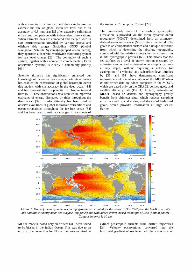
by [35] and [51] have demonstrated significant

improvement of spatial resolution of the MDOT when

in situ drifter data are added compared to the MDOT,

which are based only on the GRACE-derived geoid and

satellite altimetry data (Fig. 1). In turn, estimates of

MDOT, based on drifters and hydrography greatly

benefit from altimeter data, which reduces sampling

error on small spatial scales, and the GRACE-derived

geoid, which provides information at large scales.

Earlier

Figure 1. Maps of mean dynamic ocean topographies calculated for the period 1993–2002 from the GRACE gravity

and satellite altimetry mean sea surface (top panel) and with added drifter-based technique of [35] (bottom panel).

Contour interval is 10 cm.

MDOT models, based only on drifters [41], were found

to be biased in the Indian Ocean. This was due to an

error in the correction for Ekman currents required to

extract geostrophic currents from drifter trajectories

[34]. Velocity observations, converted into the

horizontal gradient of sea level, add the scales smaller

than the ones resolved by the current model of the

geoid, so that the combined products (Fig. 1b) better

describe many complex current systems associated with

sharp fronts. At present, the GRACE mean geoid model

is accurate at 1–2 cm level at 200 km (half-wavelength).

The anticipated geoid model from GOCE is expected to

have a similar accuracy but at a much finer wavelength

of 100 km. Therefore, further improved accuracy of

MDOT is expected in the near future [29].

The observation of the mesoscale and sub-mesoscale

variability and geostrophic currents requires either an

extensive constellation of nadir-pointing altimeters, or,

optimally using at least one wide-swath instrument,

such as the SWOT Mission [1], [15] and [16]. Such

instrumentation is also required for the more complete

exploitation of altimetry in coastal areas [11], and

global surface water hydrology [1]. The observations of

total land (including ice-sheets, mountain glaciers and

ice caps) water storage change, or the absolute water

storage exchange between the land/ice surface and the

ocean, are critically important to quantify the freshwater

budget and its effect on general ocean circulation and

global sea level change [7], [30] and [36]. The cited

studies address the former quantity, i.e. land storage

change, which is demonstrated to be potentially

quantifiable at the appropriate temporal and spatial

resolutions by GRACE, satellite altimetry and

hydrography data including Argo.

In coastal areas, which are often densely populated,

geodetic techniques (e.g. tide gauges, GNSS, DORIS

(Détermination d‟Orbite et Radiopositionnement

Intégrés par Satellite)) are crucial for monitoring

changes in sea surface height and land surface height.

Such observations provide critical constraints on models

of the local, regional, and global processes that drive

local sea level change. In the long term, these

observations will be a crucial component of information

required by decision and policy makers for mitigating

and adapting to the coastal impact of climate change

[47] caused by regional and global sea level rise [8].

3. GETTING TO THE BOTTOM OF THINGS:

OCEAN BOTTOM PRESSURE, INTERMEDIATE-

DEPTH CIRCULATION, AND OCEAN HEAT

STORAGE

A basic tenet of measurement theory is to avoid

wherever possible measuring a small signal as the

difference of two large signals. Of the triad: sea level,

density, ocean bottom pressure (OBP), the smallest

signal is OBP [3], making it particularly attractive to

monitor this quantity directly. Gradients of the ocean

bottom pressure across major currents determine bottom

geostrophic currents and can be used to infer variations

in barotropic mass transport. In situ OBP sensors tend to

have slowly varying datum fluctuations, which make

determining long-term changes in transport difficult.

Multi-year time series of OBP is difficult to obtain and

most in situ measurements have typically been restricted

to deployments of one year at a limited number of

locations, although with present-day technology it is

possible to deploy for 2 to 5 years; see e.g. [22], [37].

[44] and [62]. Consequently, long time series are only

obtained by redeploying instruments at the same

location. The combination of short time records for each

instrument and their different drifts makes studying

interannual and longer variability difficult or nearly

impossible.

At present, GRACE measures the global time-variable

gravity field with monthly sampling (or finer) and

spatial scale as fine as 250 km or longer, depending on

latitude and location. The ocean measurements have

lower signal-to-noise ratios than the measurements over

land or ice-sheets. GRACE has yielded monthly maps

of mass changes since April 2002. These data can be

used to infer time-variable ocean bottom pressure on

similar time- and space–scales; see e.g. [26] and [55].

The accuracy of measurements yields suitable signal-to-

noise ratios at mid to high latitudes [5], [12] and [38].

Because GRACE data are global, one can compute

transport variability across a much larger area, and

determine how the transport is changing from one area

Figure 2. Seasonal averages of the monthly GRACE (Rel. 4, 300 km radius Gaussian filter) Arctic Ocean bottom

pressure anomalies in cm water equivalent from August 2002 to May 2008, relative to the temporal mean from 2003 to

2006 [44].

to another, as [6] and [65] have done for the Antarctic

Circumpolar Current. Because of the long, nearly

continuous record, GRACE data have also been used to

demonstrate significant low-frequency fluctuations in

OBP: in the Arctic at seasonal [44] (Fig. 2) and

interannual [38] time-scales in the North Pacific

(Figs. 3 and 4) [53] and [10] that are likely related to

transport changes and ENSO (El Niño/Southern

Oscillation) events; and in the Southern Ocean [28] that

dominate sea level change. However, the use of

GRACE data to study changes in large-scale, low-

frequency volume transport has not yet been fully

exploited The gradient of OBP fluctuations and the near

bottom currents they produce are directly related to

changes in sea surface elevation only in a barotropic

flow, where pressure gradients are uniform with depth

and directly relate to mass transport variations.

However, the relationship is not so simple in a

baroclinic environment, where changes in pressure

gradients occur due to spatial differences in temperature

and/or salinity, which vary with depth. In fact, model

results suggest that at long time-scales OBP is strongly

related to density variations that induce baroclinic

currents [54] and [38] (Fig. 5). Thus to properly resolve

fluctuations in the transports of mass, heat, and

freshwater, one must combine GRACE with altimetric

data and in situ measurements of T and S (Temperature

and Salinity), from either hydrography or Argo floats.

Although the Argo program is now making global

monthly observations of upper ocean temperature and

salinity at a resolution of about 3°, combinations of

satellite altimetry and GRACE data to estimate changes

in steric sea level and heat storage (see e.g. [9] and [26])

may prove to be important. The Argo floats give

accurate measures of the temperature and salinity

profile for a particular location in the ocean. This will

include both the long-wavelength signal as well as

signals from very short-wavelength fluctuations, such as

eddies. In some areas of the ocean (notably the western

boundary currents and the Antarctic Circumpolar

Current), small-scale, energetic eddies can obscure the

Figure 3. GRACE-observed Ocean-Bottom-Pressure oscillation in North Pacific is shown to link the tropical ENSO and

the Aleutian Low through an atmospheric bridge [53].

Figure 4. GRACE-observed ocean bottom pressure variations in North Pacific compared with steric-corrected (Argo)

satellite altimetry [10].

Figure 5. Bottom pressure at the North Pole from GRACE Releases 1 and 4 along with averages of in situ Arctic

Bottom Pressure Recorder records. Absolute values are arbitrary and have been set to zero for Release 4. Other record

averages are matched to Release 4. The interannual trends in steric pressure anomalies due to ocean mass changes

from upper ocean hydrographic observations account for a significant part of the GRACE trends and in agreement with

[38], [53] and [54]

longer wavelength signal. The distribution and number

of floats will never be sufficient to fully reduce this type

of aliasing.

Although the Argo program is now making global

monthly observations of upper ocean temperature and

salinity at a resolution of about 3°, combinations of

satellite altimetry and GRACE data to estimate changes

in steric sea level and heat storage (see e.g. [9] and [26])

may prove to be important. The Argo floats give

accurate measures of the temperature and salinity

profile for a particular location in the ocean. This will

include both the long-wavelength signal as well as

signals from very short-wavelength fluctuations, such as

eddies. In some areas of the ocean (notably the western

boundary currents and the Antarctic Circumpolar

Current), small-scale, energetic eddies can obscure the

longer wavelength signal. The distribution and number

of floats will never be sufficient to fully reduce this type

of aliasing.

More importantly, the combination of altimetry and

GRACE should more accurately represent the long-

wavelength steric sea level. Thus, the altimetry-GRACE

combination will be important as a fundamental

reference to which information from the Argo floats can

be added. In addition to the difference in horizontal

resolution, there is a difference in vertical sampling. The

current array of Argo floats only take measurements to a

depth of 2,000 m, meaning there are several thousand

meters of ocean depth not covered in many areas. The

combination of GRACE and altimeter measurements,

however, represents temporal changes in the vertical

integral of density from the surface to the ocean floor.

It may therefore be possible to detect changes in the

deep ocean by combining all three data sets. While most

seasonal to interannual fluctuations will be confined to

the upper 1,000 m of the ocean, there is evidence that

temperature fluctuations on periods of 10-years or more

can occur in the deep ocean below 2,000 m [32].

Furthermore, sampling of the deep ocean has

historically been inadequate [20] and there is currently

no plan for comprehensive in situ sampling of the deep

ocean. In addition, there are issues involving

depth-dependent instrument biases in XBT (XBT

(Expendable Bathythermograph) and MBT (Mechanical

Bathythermograph) data and various investigators have

different estimates of (upper) ocean warming and the

corresponding thermosteric sea level rise. Estimates of

thermal expansion of the upper ocean vary for the last

50 years from 0.24 mm/yr to 0.6 mm/yr [2], [13], [20]

[25] and [56].

Separating the globally averaged sea level rise into its

two key components, water mass addition and density

changes, allows for a comparison of the global water

budget with estimates of ice melt from glaciers and ice

sheets. This is a very difficult computation, which is

complicated by the correlation of the spatial and

temporal characteristics of some of the contributions. It

requires extreme accuracy [7], [31], [33], [43], [45] and

[57], and current estimates disagree at the ~1 mm/yr

level. However, much of this is related to the glacial

isostatic adjustment (GIA) forward models that are used

as correction to the GRACE data and the short time

series available for the study. These GIA models,

expressed in terms of oceanic mass variations, have an

averaged signal of 1–2 mm/yr over the ocean, indicating

significant discrepancy depending on the choice of the

model. In addition, the models also predicted a

correction on the same magnitude as the observed

GRACE ocean mass signals. With longer time series

and other geodetic measurements, there is potential to

improve GIA models. Also, since GIA corrections are

quite large for GRACE but not for altimetry, long time-

series of altimetry, GRACE, and Argo can be used to

evaluate different GIA models. Here again, the

combination of GRACE, altimetry and Argo floats is a

novel approach to provide an improved quantification of

the state of the ocean. Moreover, geodetic observations

(including GRACE, gravimetry, laser and radar

altimetry, and InSAR and Wide-Swath altimeters) also

provide the means to determine mass changes in the ice

sheets, glaciers and land water storage and discharge. In

fact, the geodetic techniques are crucial in establishing a

global mass balance in the water cycle as an additional

constraint for changes in the ocean mass.

Geostrophic ocean currents reflect a balance between

pressure gradients and the Coriolis force. While surface

geostrophic currents, which have both baroclinic and

barotropic components, are defined by the dynamic

surface topography, below the sea surface. The

baroclinic component due to horizontal density

gradients tends to diminish the currents and turn their

direction with depth. Combining the recently available

high-quality MDOT with satellite altimetry and CTD-

profiles from more than 3,000 Argo floats now allows

one to derive the absolute dynamic height (ADH) and

assess geostrophic currents in the upper 2,000 meters of

the ocean. This is an idea first proposed nearly 30 years

ago [63], demonstrated during the World Ocean

Circulation Experiment (WOCE) using hydrographic

data [17], and that is now possible in part due to the

innovative geodetic satellite missions and techniques, in

particular from the contribution of GOCE to the

improved quantification of the absolute general ocean

circulation [29]. Recently, a preliminary monthly

gridded dataset was made available at the Asia-Pacific

Data Research Center (APDRC). Of particular interest

are the studies of the vertical structure of baroclinic

currents [57] and [58].

4. EMERGING GEODETIC TECHNOLOGY &

CHALLENGE SATELLITE ALTIMETRY:

Because of its enormous value for ocean monitoring,

altimetry will become part of operational satellite

systems such as the Jason series and the Sentinel series

of European Union/European Space Agency (EU/ESA)

Global Monitoring for Environment and Security

(GMES) [60]. Significant new technology developments

include the Delay/Doppler altimeter [50] with an earlier

version of the instrument design, the

SAR/Interferometric Radar Altimeter (SIRAL) system

onboard of the CryoSat mission, and the wide-swath

InSAR radar altimetry instrument, onboard of SWOT.

An emerging technique is GNSS reflectrometry, i.e. the

analysis of the travel time of signals emitted by GNSS

satellites, reflected at the ocean surface and received in

airplanes or low orbiting satellites. A number of groups

are currently investigating the accuracy of such a

measurement concept. First results look promising but

the technique is far from being well established.

Satellite gravimetry: GRACE is currently providing

very accurate monthly time series of changes in the

Earth‟s wavelength gravity field. This adds a new – and

very central – parameter set to the study of global

change phenomena such as de-glaciation in the large ice

shields of Antarctica and Greenland, sea level rise, or

the variations of the global water cycle. GOCE will

deliver a global static gravity field and geoid with

unprecedented accuracy and spatial resolution. It will in

particular serve as reference for global ocean circulation

studies by altimetry.

To completely understand the physical processes of

the Earth under a warming climate, continuous

measurements of gravity changes in the form of an

ongoing series of satellites are necessary. Workshops

on the future satellite gravimetry missions were

held at ESA/ESTEC (European Space Research and

Technology Centre) [27], and at the Technische

Universität Graz in 2007 and 2009, respectively.

To facilitate a long-term commitment to satellite

gravity missions, the 2009 Graz workshop

(http://www.igcp565.org/workshops/Graz.) was co-

organized by IAG/GGOS and Global Earth Observation

(GEO) in cooperation with Space Agencies to formulate

and agree on a roadmap for future gravity satellite

missions. The Workshop participants agreed on a

roadmap for future gravity satellite missions. The

strategic target for this roadmap is to accomplish “a

multi-decade, continuous series of space-based

observations of changes in the Earth's gravity field

begun with the GRACE mission, and leading, before

2020, to satellite systems capable of monitoring

temporal gravity field from global down to regional

spatial scales and on time scales of two weeks or

shorter. This data set will contribute to an integrated

and sustained operational observing system for mass

redistribution, to monitor natural hazards and their

potential early detection, to support global water

resource management, and to improve understanding of

climate change.”

In addition, the Graz Workshop participants supported

the idea of a GRACE stopgap or continuity mission

based on the present GRACE technology, with

emphasis on the continuation of time series of global

gravity changes with a minimum gap. Current estimate

for the end of the GRACE mission is 2013, requiring a

high priority GRACE Continuity satellite mission

launch soon after that time, e.g. ~2015. The U.S. NRC

Decadal Survey lists the GRACE follow-on (laser

interferometry) as one of its recommended missions for

the next 15 years, but in the 2017–2020 time frame.

This would mean a gap of 5–8 years in time variable

gravity and OBP, with unacceptable negative impacts

on all scientific objectives and applications described

above. If this delay occurs, we will have to rely on

optimum use of a greatly expanded program of in situ

observations.

The medium term priority should be focused on higher

precision and higher resolution gravity in both space

and time. This step requires (1) the reduction of the

current level of aliasing of high-frequency geophysical

signals including ocean tides and atmosphere loading

into the gravity field time series (2) the mitigation of

geographically-correlated high spatial frequency

distortions (caused primarily by the peculiar non-

isotropic sensitivity of a single pair of low-low SST

(Satellite to Satellite Tracking) measurement system and

(3) the improvement of the separability of the observed

geophysical signals. Elements of a strategy in this

direction are the use of two or more pairs of satellites,

probably with one pair in a moderate inclination orbit,

and efforts to improve the background models, for

example, perturbations on the satellites due to

atmosphere loading and ocean tides. This will open the

door to an efficient use of improved sensor systems,

such as laser interferometry ranging systems and active

angular and drag-free control systems. Other

experimental and longer-term sensor technologies that

potentially shows promise for gravity observations

include cold-atom quantum gravity sensors and ultra-

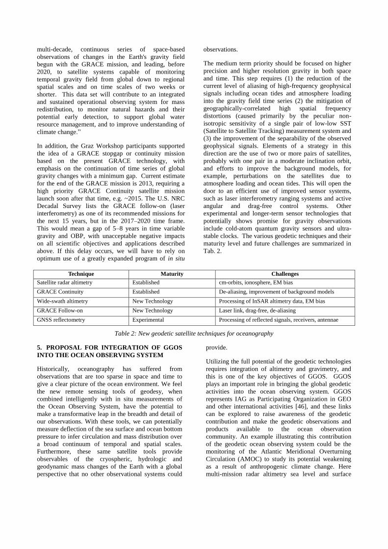
stable clocks. The various geodetic techniques and their

maturity level and future challenges are summarized in

Tab. 2.

Technique Maturity Challenges

Satellite radar altimetry Established cm-orbits, ionosphere, EM bias

GRACE Continuity Established De-aliasing, improvement of background models

Wide-swath altimetry New Technology Processing of InSAR altimetry data, EM bias

GRACE Follow-on New Technology Laser link, drag-free, de-aliasing

GNSS reflectometry Experimental Processing of reflected signals, receivers, antennae

Table 2: New geodetic satellite techniques for oceanography

5. PROPOSAL FOR INTEGRATION OF GGOS

INTO THE OCEAN OBSERVING SYSTEM

Historically, oceanography has suffered from

observations that are too sparse in space and time to

give a clear picture of the ocean environment. We feel

the new remote sensing tools of geodesy, when

combined intelligently with in situ measurements of

the Ocean Observing System, have the potential to

make a transformative leap in the breadth and detail of

our observations. With these tools, we can potentially

measure deflection of the sea surface and ocean bottom

pressure to infer circulation and mass distribution over

a broad continuum of temporal and spatial scales.

Furthermore, these same satellite tools provide

observables of the cryospheric, hydrologic and

geodynamic mass changes of the Earth with a global

perspective that no other observational systems could

provide.

Utilizing the full potential of the geodetic technologies

requires integration of altimetry and gravimetry, and

this is one of the key objectives of GGOS. GGOS

plays an important role in bringing the global geodetic

activities into the ocean observing system. GGOS

represents IAG as Participating Organization in GEO

and other international activities [46], and these links

can be explored to raise awareness of the geodetic

contribution and make the geodetic observations and

products available to the ocean observation

community. An example illustrating this contribution

of the geodetic ocean observing system could be the

monitoring of the Atlantic Meridional Overturning

Circulation (AMOC) to study its potential weakening

as a result of anthropogenic climate change. Here

multi-mission radar altimetry sea level and surface

geostrophic current velocities, GRACE-derived ocean

bottom pressure and GRACE-observed land and ice

melt water mass fluxes, GOCE-measured geoid and

MODT, mooring arrays, and data from tide gauges and

Argo, collectively can establish a monitoring system to

potentially monitor the present-day evolution of the

AMOC. Another scientific application is to estimate

strait and inter-ocean transport using the combined

altimetry sea surface height and GRACE ocean bottom

pressure data [48] and [53]. These applications are of

fundamental interest to address research problems in

oceanography [18] and climate change [19] and [21].

The improvement and the constraints of the GIA

processes resulting from the Last Glacial Maximum

and to a lesser extent, the Little Ice Age, have

significant impact on accurate estimates of oceanic

mass variation. It is recommended that the GIA

forward models be improved and their error

characteristics be quantified when they are used to

correct GIA effects integrated (geodetic and in situ)

measurements to quantify oceanic mass variations and

global water cycles and their impact on ocean

freshening and circulation.

There are serious challenges to be sure. The GRACE

measurements have demonstrated its importance for

ocean monitoring. Now the gap between GRACE and

the GRACE follow-on is seen as a critical problem.

GRACE has a nominal mission life span of 5 years

(2002–2007), however, its extraordinary performance

provides an opportunity to extend its mission to 2013.

The GRACE follow-on mission is expected to be

launched in the 2017–2020 time frame. There is a

reasonable good chance that a GRACE Continuity

mission to minimize the data gap between GRACE and

its follow-on would be launched around 2015. It is

recommended that the planned GRACE Continuity

mission would have potential incremental

improvements such as mitigation of temporal and

spatial aliasing and improvement of spatial resolutions

by flying more than one pairs of GRACE-type

satellites in a constellation, at distinct inclinations and

at lower altitudes.

Much of the progress in ocean observation ultimately

will depend on the success of the global geodetic

community behind GGOS to maintain the accurate and

long-term reference frame required for Earth

observation. Continued refinements to the terrestrial

reference frame depend on adequate coverage and

collocation of geodetic techniques, including VLBI and

satellite laser ranging. Closing the current large

geographical gaps in the global network of core

geodetic stations is therefore a high priority of GGOS,

as is the identification and maintenance of the core

geodetic infrastructure required for the determination

of an ITRF that meets the requirements of global

change research, including those of oceanography [46,

Chapter 11]. The accuracy and stability of the ITRF,

for example, have significant impacts on monitoring

sea level change and are therefore affecting the

determination of the absolute ocean circulation. It is

recommended that the drift of the ITRF be monitored

to be <0.1 mm/yr. Finally, future satellite altimeters

should be designed to meet at least the 0.3 mm/yr

accuracy in global sea level needed for climate studies

that is currently achieved by extensive post-flight

calibration that takes months or sometimes years [8].

There are key in situ measurements that we will

particularly value as part of the ocean observing

system. These include: (1) independent observations of

sea surface height (i.e. tide gauges, most equipped with

GNSS receivers), that can validate and extend the

satellite altimeter results (2) hydrography (e.g. Argo

floats) that would extend the coverage and sampling to

deep ocean (>2,000 m) and that validates and details

the mass distribution changes inferred from satellite

altimetry and gravity (3) in situ bottom pressure arrays,

including those in the polar ocean, that validates the

satellite gravity-based measurements and could

improve our ability to de-alias the satellite gravity and

altimetry data for tidal and other high frequency

motions and (4) Lagrangian drifter measurements with

which to compare velocity solutions over broad areas.

It is recommended that the Argo arrays be enhanced to

cover the commensurate observational sampling in the

deeper part of the ocean (>2,000 m).

Perhaps one of the most important outcomes of this

white paper and OceanObs'09 would be the thorough

integration of geodesy into the ocean observing system

of the future. The ocean science community is on the

verge of putting together a larger and ever improving

array of observations. If geodetic techniques are an

integral part of the observing system, the tools of

geodesy can provide unprecedented spatial and

temporal continuity to the physical observations and

consequent insights into the behaviour of the world

ocean.

6. ACKNOWLEDGEMENT

We thank Carl Wunsch for his constructive comments,

which have improved this manuscript. Peter H. Luk‟s

help on text-processing of the manuscript is gratefully

acknowledged.

7. REFERENCES

[1] Alsdorf, D., Rodriguez, E, & Lettenmaier, D. (2007).

Measuring surface water from space, Rev. Geophys.,

45, doi:10.1029/2006RG000197, 2007.

[2] Antonov, J., S. Levitus, S. & Boyer, T. (2005). Steric

variability of the world ocean, 1955-2003, Geophys.

Res. Lett., 32(12), L12602,

doi:10.1029/2005GL023112.

[3] Bingham, R. J. & Hughes, C. W. (2008). The

relationship between sea-level and bottom pressure

variability in an eddy-permitting ocean model.

Geophys. Res. Lett., 35, L03602,

doi:10.1029/2007GL032662.

[4] Blewitt, G., Altamimi, Z. Davis, J. Gross, R. Kuo, C.

Lemoine, F. Neilan, R. Plag, H.P. Rothacher, M.

Shum, C. Sideris, M. Schoene, T. Tregoning, P. &

Zerbini, S. (2006). Geodetic observations and global

reference frame contributions to understanding sea

level rise and variability, in Understanding Sea-level

Rise and Variability, A World Climate Research

Programme Workshop and a WCRP contribution to

the Global Earth Observation System of Systems, 6–9

June 2006, UNESCO, Paris, T. Aarup, J. Church, S.

Wilson, & P. Woodworth (Ed.), 127–143, WCRP,

World Meterological Organization, Paris.

[5] Böning, C., Timmermann, R. Macrander, A. &

Schröter, J. (2008). A pattern-filtering method for the

determination of ocean bottom pressure anomalies

from GRACE solutions, Geophys. Res. Lett., 35,

L18611, doi:10.1029/2008GL034974.

[6] Böning, C., Timmermann, R. Danilov, D. & Schröter,

J. (2009). On the representation of transport

variability of the Antarctic Circumpolar Current in

GRACE gravity solutions and numerical ocean model

simulations, In Flechtner F, Gruber T, Güntner A,

Mandea M, Rothacher M, Schöne T, Wickert J (eds.)

Satellite Geodesy and Earth System Science,

Springer-Verlag, Berlin, Heidelberg.

[7] Cazenave, A., Dominh, K. Guinehut, S, Berthier, E.

Llovel, W, Ramillien, R, Ablain, M. & Larnicolm, G.

(2009). Sea level budget over 2003-2008: A

reevaluation from GRACE space gravimetry, satellite

altimetry and Argo, Global and Planetary Change,

65, 83-88, doi:10.1016/j.gloplacha.2008.10.004.

[8] Cazenave, A. & Co-Authors (2010). "Sea Level Rise -

Regional and Global Trends" in these proceedings

(Vol. 1), doi:10.5270/OceanObs09.pp.11.

[9] Chambers, D.P., Cipollini, P. Fu, L.L. Hurell, J.W.

Merrifield, M. Nerem, R.S. Plag, H.P. Shum, C.K.

Willis, J. & Chambers, D.P. (2006). Observing

seasonal steric sea level variations with GRACE and

satellite altimetry, J. Geophys. Res., 111 (C3),

C03010, doi:10.1029/2005JC002914.

[10] Chambers D.P. & Willis J.K. (2008). Analysis of large-

scale ocean bottom pressure variability in the North

Pacific, J. Geophys. Res., 113, C11003,

doi:10.1029/2008JC004930.

[11] Cipollini, P. & Co-Authors (2010). "The Role of

Altimetry in Coastal Observing Systems" in these

proceedings (Vol. 2),

doi:10.5270/OceanObs09.cwp.16.

[12] Dobslaw, H., & Thomas, M. (2007). Simulation and

observation of global ocean mass anomalies, J.

Geophys. Res., 112, C05040,

doi:10.1029/2006JC004035.

[13] Domingues, C., Church, J. White, N. Gleckler, P.

Wijffels, S. Barker, P. & Dunn, J. (2008). Improved

estimates of upper-ocean warming and multi-decadal

sea-level rise, Nature, 453, doi:10.1038/nature07080.

[14] Fu, L.L. & Cazenave, A. (2000). Satellite altimetry and

Earth sciences: a handbook of techniques and

applications, Academic Press, San Diego, CA.

[15] Fu, L.L. (2007). Objectives and requirements of SWOT

for observing the oceanic mesoscale variability,

NASA SWOT Workshop, Scripps Institute of

Oceanography, April 28–May 1.

[16] Fu, L. & Co-Authors (2010). "The Surface Water and

Ocean Topography (SWOT) Mission" in these

proceedings (Vol. 2),

doi:10.5270/OceanObs09.cwp.33.

[17] Ganachaud, A., & Wunsch, C. (2000). Improved

estimates of global ocean circulation, heat transport

and mixing from hydrographic data, Nature, 408,

453–457.

[18] Godfrey, J.S. (1996). The effect of the Indonesian

throughflow on ocean circulation and heat exchange

with the atmosphere: A review, J. Geophy. Res., 101,

12217-12237.

[19] Gordon, A.L., Susanto, R.D. & Vranes, K. (2003). Cool

Indonesian Throughflow as a consequence of

restricted surface layer flow, Nature, 425, 824-828.

[20] Gouretski, V., & Koltermann, K.P. (2007). How much

is the ocean really warming? Geophys. Res. Lett., 34:

L01610, doi:10.1029/2006GL027834.

[21] Hansen, B., Turrell, W.R. & Osterhus, S. (2001).

Decreasing overflow from the Nordic seas into the

Atlantic Ocean through the Faroe Bank channel since

1950, Nature, 411, 927-930.

[22] Hughes, C.W., Woodworth, P.L. Meredith, M.P.

Stepanov, V. Whitworth, T. & Pyne, A.R. (2003).

Coherence of Antarctic sea levels, Southern

Hemisphere Annular Mode, and flow through Drake

Passage. Geophys. Res. Lett, 30(9), 1464,

doi:10.1029/2003GL017240.

[23] IOC, Global Sea Level Observing System

Implementation Plan 2009, (edited by M. Merrifield).

Intergovernmental Oceanographic Commission, in

preparation.

[25] Ishii, M., & Kimoto, M. (2009). Reevaluation of

historical ocean heat content variations with time-

varying XBT and MBT depth bias corrections, J.

Oceanography, 65, 287–299.

[26] Jayne, S. R. (2006), Circulation of the North Atlantic

Ocean from altimetry and the Gravity Recovery and

Climate Experiment geoid, J. Geophys. Res., 111,

C03005, doi:10.1029/2005JC003128.

[27] Koop, R., & Rummel, R. (2007). The future of satellite

gravimetry, Workshop on the Future of Satellite

Gravimery Report, ESTEC, Noordwijk, The

Netherlands, April 12–13.

[28] Kuo, C., Shum, C. Guo, J. Yi, Y. Braun, A. Fukumori,

I. Matsumoto, K. Sato, T. & Shibuya, K. (2008).

Southern Ocean Mass Variation Studies Using

GRACE and Satellite Altimetry, Earth Planets and

Space, 60, 1–9.

[29] Legrand, P. (2005). Future Gravity Missions and

Quasi-steady Ocean Circulation, Earth, Moon, and

Planets, 94(1–22), doi:10.1007/s11038-004-7606-9.

[30] Lettenmaier D. & Milly, C. (2009). Land waters and

sea level, Nature, 2, 452–454.

[31] Leuliette, E.W., & Miller, L. (2009). Closing the sea level

rise budget with altimetry, Argo, and GRACE, Geophys.

Res. Lett., 36, L04608, doi:10.1029/2008GL036010.

[32] Levitus, S., Antonov, J. & Boyer, T. (2005). Warming of

the world ocean, 1955–2003. Geophys. Res. Lett., 32:

L12602, doi:10.1029/2005GL023112.

[33] Lombard, A., Garcia, D. Ramillien, G. Cazenave, A.

Biancale, R. Lemoine, J.M. Flechtner, F. Schmidt, R.

& Ishii, M. (2007). Estimation of steric sea level

variations from combined GRACE and Jason-1 data,

Earth and Planetary Science Letters, 254, 194–202,

doi:10.1016/j.epsl.2006.11.035.

[34] Maximenko, N.A., & Niiler, P.P. (2005). Hybrid

decade-mean global sea level with mesoscale

resolution. In Saxena, N. (Ed.) Recent Advances in

Marine Science and Technology, 2004. Honolulu:

PACON International, 55–59.

[35] Maximenko, N., Niiler, P. Rio, M.H. Melnichenko, O.

Centurioni, L. Chambers, D. Zlotnicki, V. &

Galperin, B. (2009). Mean dynamic topography of

the ocean derived from satellite and drifting buoy

data using three different techniques. J. Atmos.

Oceanic Tech., 26(9), 1910–1919.

[36] Milly, P.C.D., Cazenave, A. Famiglietti, J. Gornitz, V.

Laval, K. Lettenmaier, D. Sahagian, D. Wahr, J. &

Wilson, C. (2009). Terrestrial water storage

contributions to sea level rise and variability,

Proceedings of the WCRP workshop „Understanding

sea level rise and variability‟, eds. J. Church, P.

Woodworth, T. Aarup and S. Wilson et al., Blackwell

Publishing, Inc.

[37] Morison, J.H. (1990). Seasonal fluctuations in the West

Spitsbergen Current estimated from bottom pressure

measurements. J. Geophys. Res., 96 (C10), 18,381-

18,395.

[38] Morison, J., Wahr, J. Kwok, R. & Peralta-Ferriz, C.

(2007). Recent trends in Arctic Ocean mass

redistribution revealed by GRACE, Geophys. Res.

Lett., 34, L07602, doi:10.1029/2006GL029016.

[39] Munk, W.H. (1997). Once again: Once again - tidal

friction, Progress in Oceanography, 40, 1–4, 7–35.

[40] Nerem, R. & Co-Authors (2010). "Observations of Sea

Level Change: What Have We Learned and What

Are the Remaining Challenges?" in these proceedings

(Vol. 2), doi:10.5270/OceanObs09.cwp.65.

[41] Niiler, P.P., Maximenko, N.A., & McWilliams, J.C.

(2003). Dynamically balanced absolute sea level of

the global ocean derived from near-surface velocity

observations, Geophys. Res. Lett., 39(22), 2164,

doi:10.1029/2003GL018628.

[42] Park, J.-H. Watts, D.R. Donohue, K.A. & Jayne, S.R.

(2008). A comparison of in situ bottom pressure array

measurements with GRACE estimates in the

Kuroshio Extension, Geophys. Res. Lett., 35, L17601,

doi:10.1029/2008GL034778.

[43] Peltier. W.R. (2009). Closure of the budget of global

sea level rise over the GRACE era: the importance

and magnitudes of the required corrections for global

glacial isostatic adjustment Quaternary Science

Reviews, Volume 28, Issues 17-18, , Pages 1658-

1674, Quaternary Ice Sheet-Ocean Interactions and

Landscape Responses,

doi:10.1016/j.quascirev.2009.04.004

[44] Peralta-Ferriz, C., J. Morison, J. Wahr, and R. Kwok,

2007, Variability of Mass in the Arctic Ocean Using

GRACE and In Situ Bottom Pressure Measurements,

Eos Transactions. AGU, 88(52), Fall Meet. Suppl.,

Abstract U21C-0624.

[45] Plag, H.P. (2006). Recent relative sea level trends: an

attempt to quantify the forcing factors, Phil. Trans.

Roy. Soc. London, A, 364, 1841-1869.

[46] Plag, H.P. & Pearlman, M. eds. (2009). The Global

Geodetic Observing System: Meeting the

Requirements of a Global Society on a Changing

Planet in 2020, Geoscience Books, Springer, Berlin,

332 pp.

[47] Plag, H.P. & Co-Authors (2010). "Observations as

Decision Support for Coastal Management in

Response to Local Sea Level Changes” in these

proceedings (Vol. 2),

doi:10.5270/OceanObs09.cwp.69.

[48] Qu, T., and Y. T. Song (2009), Mindoro Strait and

Sibutu Passage transports estimated from satellite

data, Geophys. Res. Lett., 36, L09601,

doi:10.1029/2009GL037314.

[49] Raney, R. (1998). The delay/Doppler radar altimeter,

IEEE Trans. Geosci. 472, Remote Sens., 36(5), 1578–

1588.

[50] Ray, R., & Mitchum, G. (1996). Surface manifestation

of internal tides generated near Hawaii, Geophys.

Res. Lett., 23(16), 2101-2104.

[51] Rio M., & Hernandez, F. (2004). A mean dynamic

topography computed over the world ocean from

altimetry, in situ measurements, and a geoid model, J.

Geophys. Res., 109, C12032,

doi:10.1029/2003JC002226.

[52] Song, Y.T. (2009). Estimation of interbasin transport

using ocean bottom pressure: Theory and model for

Asian marginal seas, J. Geophys. Res., 111, C11S19,

doi:10.1029/2005JC003189.

[53] Song, Y.T. & Zlotnicki, V. (2008). The subpolar ocean-

bottom-pressure oscillation and its links to ENSO,

Int. J. Remote Sensing, Vol. 29 (21), 6091–6107.

[54] Vinogradova, N., Ponte, R. & Stammer, D. (2007).

Relation between sea level and bottom pressure and

the vertical dependence of oceanic variability,

Geophys. Res. Lett., 34, L03608,

doi:10.1029/2006GL028588.

[55] Wahr, J., Molenaar, M. & Bryan, F. (1998). Time-

variability of the Earth‟s gravity field: Hydrological and

oceanic effects and their possible detection using

GRACE, J. Geophys. Res., 103, 32,205–30,229.

[56] Wijffels, S.E., Willis, J. Domingues, C.M. Barker, P.

White, N.J. Gronell, A. Ridgway, K. & Church, J.A.

(2008). Changing expendable bathythermograph fall

rates and their impact on estimates of thermosteric

sea level rise, J. Climate, 21, 5657–5672.

[57] Willis, J.K., & Fu, L.L. (2008). Combining altimeter

and subsurface float data to estimate the time-

averaged circulation in the upper ocean. J. Geophys.

Res., 113, C1207, doi:10.1029/2007JC004690.

[58] Willis, J.K., Roemmich, D. & Cornuelle, B. (2003).

Combining altimetric height with broadscale profile

data to estimate steric height, heat storage, subsurface

temperature, and sea-surface temperature variability.

J. Geophys. Res., 108(C9), 3292,

doi:10.1029/2002JC001755.

[59] Willis, J.K., Chambers, D.P. & Nerem, R.S. (2008).

Assessing the globally averaged sea level budget on

seasonal to interannual timescales, J. Geophys. Res.,

113, C06015, doi:10.1029/2007JC004517.

[60] Wilson, S., & Parisot, F. (2008). Proc. CEOS Ocean

Surface Topography Constellation Strategic

Workshop, Assmannshausen, Germany, 29–31

January.

[61] Wilson, S., W, Abdalti, D. Alsdorf, J. Benveniste, H.

Bonekamp, G. Cogley, M. Drinkwater, L.-L. Fu, R.

Gross, B. Haines, E. Harrison, G. Johnson, M.

Johnson, J. LaBrecque, E. Lindstrom, M. Merrifield,

L. Miller, E. Pavlis, S. Piotrowicz, D. Roemmich, D.

Stammer, R. Thomas, E. Thouvenot, and P.

Woodworth (2010), "Observing Systems Needed to

Address Sea-level Rise and Variability", Blackwells

Pub., Eds. J. A. Church, P. L. Woodworth, T. Aarup

and W. S. Wilson, London, doi:10.1007/s11625-008-

0042-4.

[62] Woodworth, P.L., Vassie, J.M. Hughes, C.W. &

Meredith, M.P. (1996). A test of the ability of

TOPEX/POSEIDON to monitor flows through the

Drake Passage, J. Geophys. Res., 101(C5), 11935–

11947.

[63] Wunsch, C., & Gaposchkin, E.M. (1980). On using

satellite altimetry to determine the general circulation

of the ocean with application to geoid improvement,

Rev. Geophys., 18, 725–745.

[64] Wunsch, C., Ponte, R.M. & Heimbach, P. (2007).

Decadal trends in sea level patterns: 1993–2004, J.

Climate, 20(24), 5889–5911.

[65] Zlotnicki, V., Wahr, J. Fukumori, I. & Song, Y.T.

(2007). Antarctic circumpolar current transport

variability during 2003-05 from GRACE, J. Phys.

Ocean., 37, 230–244.