GRC Transactions, Vol. 38, 2014

425

Geochemistry Sampling for Traditional and Multicomponent Equilibrium Geothermometry in Southeast Idaho

Cody Cannon1,2, Thomas Wood1,2, Ghanashyam Neupane2,3, Travis McLing2,3, Earl Mattson3, Patrick Dobson4, and Mark Conrad4

1University of Idaho-Idaho Falls, Idaho Falls ID2Center for Advanced Energy Studies, Idaho Falls ID

3Idaho National Laboratory, Idaho Falls ID4Lawrence Berkeley National Laboratory, Berkeley CA

cann8218@vandals.uidaho.edu

KeywordsEastern Snake River Plain, geothermal, geothermometry, geo-chemistry, heat flow, RTEst, MEG

ABSTrACT

The Eastern Snake River Plain (ESRP) is an area of high re-gional heat flux due the movement of the North American Plate over the Yellowstone Hotspot beginning ca.16 Ma. Temperature gradients between 45-60 ̊ C/km (up to double the global average) have been calculated from deep wells that penetrate the upper aquifer system (Blackwell 1989). Despite the high geothermal potential, thermal signatures from hot springs and wells are ef-fectively masked by the rapid flow of cold groundwater through the highly permeable basalts of the Eastern Snake River Plain aquifer (ESRPA) (up to 500+ m thick). This preliminary study is part of an effort to more accurately predict temperatures of the ESRP deep thermal reservoir while accounting for the ef-fects of the prolific cold water aquifer system above. This study combines the use of traditional geothermometry, mixing models, and a multicomponent equilibrium geothermometry (MEG) tool to investigate the geothermal potential of the ESRP. In March, 2014, a collaborative team including members of the University of Idaho, the Idaho National Laboratory, and the Lawrence Berkeley National Laboratory collected 14 thermal water samples from and adjacent to the Eastern Snake River Plain. The preliminary results of chemical analyses and geothermometry applied to these samples are presented herein.

1. Introduction

High thermal fluxes in the ESRP were first documented in the early 1970’s (Brott et al., 1976). Heat flow values of 110 mW/m2 have been calculated below the ESRPA and values over 150 mW/m2 have been projected for depths to 6 km (Blackwell and Richards, 2004). Yet, to date, geothermal exploration in the area has had little success due to the masking of the geothermal systems by a huge volume of cold groundwater moving through

the ESRPA, which originates as snowmelt from the Yellowstone Plateau and surrounding mountain basins through the overlying the prolific ESRPA. The Idaho National Laboratory (INL), the University of Idaho – Idaho Falls (UI-IF), and Lawrence Berkley National Laboratory (LBNL) are partnering on a project that will improve upon conventional geothermometry and help identify hidden geothermal reservoirs beneath the ESRPA. This project is aimed at applying traditional (cation and silica), isotopic, and multicomponent equilibrium geothermometry coupled with mix-ing models to waters throughout the ESRP and southern Idaho.

Although there have been several reported water compositions (e.g., Ross, 1971; Young and Mitchell, 1973; Ralston et. al., 1981; Lewis and Young, 1982; Wood and Low, 1988; Parliman and Young, 1992; Mariner et al., 1991, 1997; McLing et al., 2002) for many ESRP springs/wells, the reported chemical analyses often do not provide complete chemical compositions. The current sampling campaign is aimed at measuring aluminum as well as several isotope compositions in spring and well waters. Here we describe the first sampling campaign conducted over five days in March of 2014 and present the preliminary results.

2. Geology and Geothermal Setting

The ESRP (Figure 1) is formed by crustal down-warping, fault-ing, and successive caldera formation that is linked to the middle Miocene to recent volcanic activities associated with the relative movement of the Yellowstone Hot Spot (Pierce and Morgan, 1992; Hughes et. al., 1999; Rodgers et. al., 2002). The ESRP consists of thick rhyolitic ash-flow tuffs, which are overlain by >1 km of Quaternary basaltic flows. The rhyolitic volcanic rocks at depth are the product of super volcanic eruptions associated with the Yellowstone Hotspot. These rocks progressively become younger to the northeast towards the Yellowstone Plateau (Pierce and Morgan, 1992; Hughes et. al., 1999). The younger basalt layers are the result of many low-volume, monogenetic shield-forming eruptions of short-duration that emanated from northwest trending volcanic rifts in the wake of the Yellowstone Hot Spot (Hughes et. al., 1999). The thick sequences of coalescing basalt flows with interlayered fluvial and eolian sediments in the ESRP constitute a

426

Cannon, et al.

very productive aquifer system above the rhyolitic ash-flow tuffs (Whitehead, 1992; Neilson et al., 2012; Shervais et al., 2013).

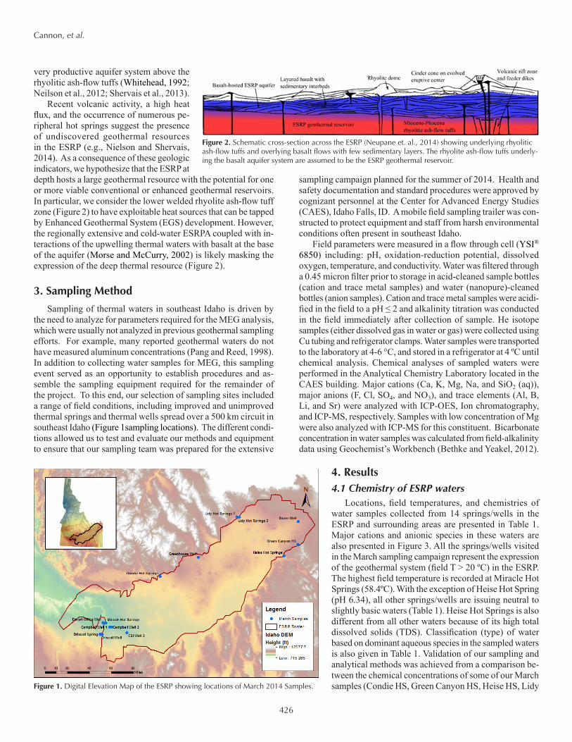
Recent volcanic activity, a high heat flux, and the occurrence of numerous pe-ripheral hot springs suggest the presence of undiscovered geothermal resources in the ESRP (e.g., Nielson and Shervais, 2014). As a consequence of these geologic indicators, we hypothesize that the ESRP at depth hosts a large geothermal resource with the potential for one or more viable conventional or enhanced geothermal reservoirs. In particular, we consider the lower welded rhyolite ash-flow tuff zone (Figure 2) to have exploitable heat sources that can be tapped by Enhanced Geothermal System (EGS) development. However, the regionally extensive and cold-water ESRPA coupled with in-teractions of the upwelling thermal waters with basalt at the base of the aquifer (Morse and McCurry, 2002) is likely masking the expression of the deep thermal resource (Figure 2).

3. Sampling Method

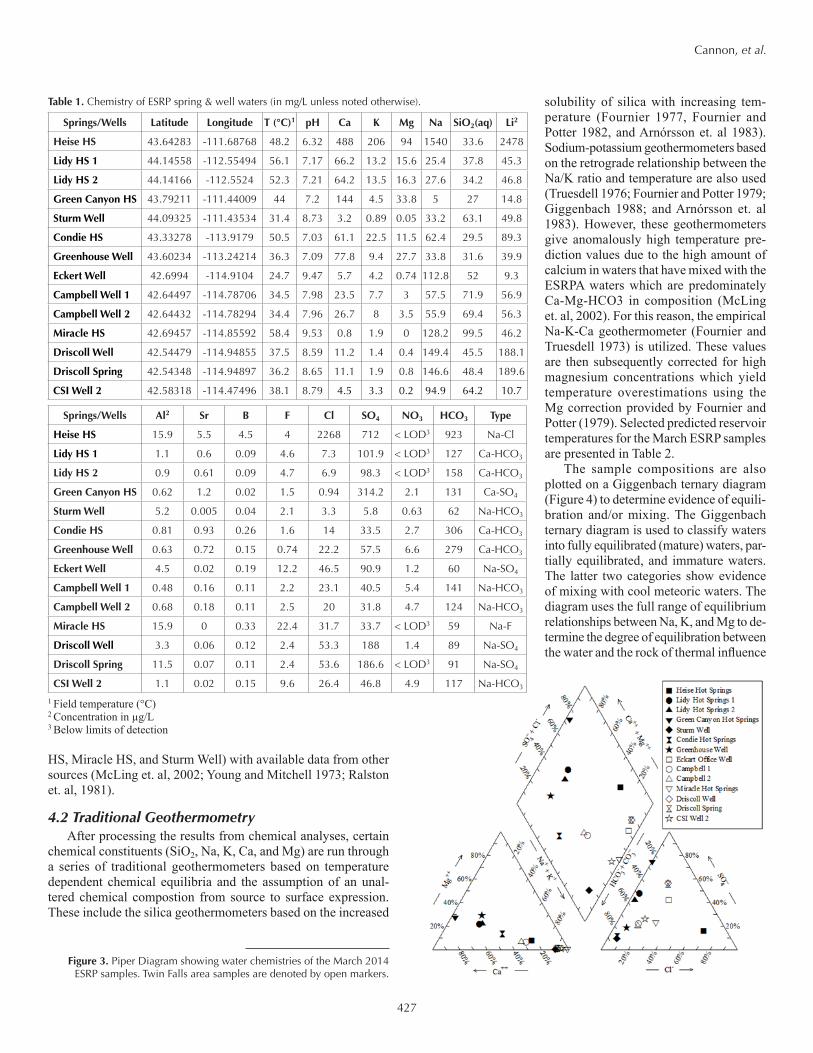
Sampling of thermal waters in southeast Idaho is driven by the need to analyze for parameters required for the MEG analysis, which were usually not analyzed in previous geothermal sampling efforts. For example, many reported geothermal waters do not have measured aluminum concentrations (Pang and Reed, 1998). In addition to collecting water samples for MEG, this sampling event served as an opportunity to establish procedures and as-semble the sampling equipment required for the remainder of the project. To this end, our selection of sampling sites included a range of field conditions, including improved and unimproved thermal springs and thermal wells spread over a 500 km circuit in southeast Idaho (Figure 1sampling locations). The different condi-tions allowed us to test and evaluate our methods and equipment to ensure that our sampling team was prepared for the extensive

sampling campaign planned for the summer of 2014. Health and safety documentation and standard procedures were approved by cognizant personnel at the Center for Advanced Energy Studies (CAES), Idaho Falls, ID. A mobile field sampling trailer was con-structed to protect equipment and staff from harsh environmental conditions often present in southeast Idaho.

Field parameters were measured in a flow through cell (YSI® 6850) including: pH, oxidation-reduction potential, dissolved oxygen, temperature, and conductivity. Water was filtered through a 0.45 micron filter prior to storage in acid-cleaned sample bottles (cation and trace metal samples) and water (nanopure)-cleaned bottles (anion samples). Cation and trace metal samples were acidi-fied in the field to a pH ≤ 2 and alkalinity titration was conducted in the field immediately after collection of sample. He isotope samples (either dissolved gas in water or gas) were collected using Cu tubing and refrigerator clamps. Water samples were transported to the laboratory at 4-6 °C, and stored in a refrigerator at 4 ºC until chemical analysis. Chemical analyses of sampled waters were performed in the Analytical Chemistry Laboratory located in the CAES building. Major cations (Ca, K, Mg, Na, and SiO2 (aq)), major anions (F, Cl, SO4, and NO3), and trace elements (Al, B, Li, and Sr) were analyzed with ICP-OES, Ion chromatography, and ICP-MS, respectively. Samples with low concentration of Mg were also analyzed with ICP-MS for this constituent. Bicarbonate concentration in water samples was calculated from field-alkalinity data using Geochemist’s Workbench (Bethke and Yeakel, 2012).

4. results4.1 Chemistry of ESRP waters

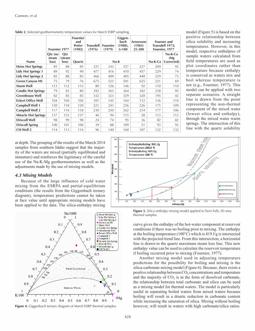
Locations, field temperatures, and chemistries of water samples collected from 14 springs/wells in the ESRP and surrounding areas are presented in Table 1. Major cations and anionic species in these waters are also presented in Figure 3. All the springs/wells visited in the March sampling campaign represent the expression of the geothermal system (field T > 20 ºC) in the ESRP. The highest field temperature is recorded at Miracle Hot Springs (58.4ºC). With the exception of Heise Hot Spring (pH 6.34), all other springs/wells are issuing neutral to slightly basic waters (Table 1). Heise Hot Springs is also different from all other waters because of its high total dissolved solids (TDS). Classification (type) of water based on dominant aqueous species in the sampled waters is also given in Table 1. Validation of our sampling and analytical methods was achieved from a comparison be-tween the chemical concentrations of some of our March samples (Condie HS, Green Canyon HS, Heise HS, Lidy Figure 1. Digital Elevation Map of the ESRP showing locations of March 2014 Samples.

Figure 2. Schematic cross-section across the ESRP (Neupane et. al., 2014) showing underlying rhyolitic ash-flow tuffs and overlying basalt flows with few sedimentary layers. The rhyolite ash-flow tuffs underly-ing the basalt aquifer system are assumed to be the ESRP geothermal reservoir.

427

Cannon, et al.

HS, Miracle HS, and Sturm Well) with available data from other sources (McLing et. al, 2002; Young and Mitchell 1973; Ralston et. al, 1981).

4.2 Traditional GeothermometryAfter processing the results from chemical analyses, certain

chemical constituents (SiO2, Na, K, Ca, and Mg) are run through a series of traditional geothermometers based on temperature dependent chemical equilibria and the assumption of an unal-tered chemical compostion from source to surface expression. These include the silica geothermometers based on the increased

solubility of silica with increasing tem-perature (Fournier 1977, Fournier and Potter 1982, and Arnórsson et. al 1983). Sodium-potassium geothermometers based on the retrograde relationship between the Na/K ratio and temperature are also used (Truesdell 1976; Fournier and Potter 1979; Giggenbach 1988; and Arnórsson et. al 1983). However, these geothermometers give anomalously high temperature pre-diction values due to the high amount of calcium in waters that have mixed with the ESRPA waters which are predominately Ca-Mg-HCO3 in composition (McLing et. al, 2002). For this reason, the empirical Na-K-Ca geothermometer (Fournier and Truesdell 1973) is utilized. These values are then subsequently corrected for high magnesium concentrations which yield temperature overestimations using the Mg correction provided by Fournier and Potter (1979). Selected predicted reservoir temperatures for the March ESRP samples are presented in Table 2.

The sample compositions are also plotted on a Giggenbach ternary diagram (Figure 4) to determine evidence of equili-bration and/or mixing. The Giggenbach ternary diagram is used to classify waters into fully equilibrated (mature) waters, par-tially equilibrated, and immature waters. The latter two categories show evidence of mixing with cool meteoric waters. The diagram uses the full range of equilibrium relationships between Na, K, and Mg to de-termine the degree of equilibration between the water and the rock of thermal influence

Table 1. Chemistry of ESRP spring & well waters (in mg/L unless noted otherwise).

Springs/Wells Latitude Longitude T (°C)1 pH Ca K Mg Na SiO2(aq) Li2

Heise HS 43.64283 -111.68768 48.2 6.32 488 206 94 1540 33.6 2478

Lidy HS 1 44.14558 -112.55494 56.1 7.17 66.2 13.2 15.6 25.4 37.8 45.3

Lidy HS 2 44.14166 -112.5524 52.3 7.21 64.2 13.5 16.3 27.6 34.2 46.8

Green Canyon HS 43.79211 -111.44009 44 7.2 144 4.5 33.8 5 27 14.8

Sturm Well 44.09325 -111.43534 31.4 8.73 3.2 0.89 0.05 33.2 63.1 49.8

Condie HS 43.33278 -113.9179 50.5 7.03 61.1 22.5 11.5 62.4 29.5 89.3

Greenhouse Well 43.60234 -113.24214 36.3 7.09 77.8 9.4 27.7 33.8 31.6 39.9

Eckert Well 42.6994 -114.9104 24.7 9.47 5.7 4.2 0.74 112.8 52 9.3

Campbell Well 1 42.64497 -114.78706 34.5 7.98 23.5 7.7 3 57.5 71.9 56.9

Campbell Well 2 42.64432 -114.78294 34.4 7.96 26.7 8 3.5 55.9 69.4 56.3

Miracle HS 42.69457 -114.85592 58.4 9.53 0.8 1.9 0 128.2 99.5 46.2

Driscoll Well 42.54479 -114.94855 37.5 8.59 11.2 1.4 0.4 149.4 45.5 188.1

Driscoll Spring 42.54348 -114.94897 36.2 8.65 11.1 1.9 0.8 146.6 48.4 189.6

CSI Well 2 42.58318 -114.47496 38.1 8.79 4.5 3.3 0.2 94.9 64.2 10.7

Springs/Wells Al2 Sr B F Cl SO4 NO3 HCO3 Type

Heise HS 15.9 5.5 4.5 4 2268 712 < LOD3 923 Na-Cl

Lidy HS 1 1.1 0.6 0.09 4.6 7.3 101.9 < LOD3 127 Ca-HCO3

Lidy HS 2 0.9 0.61 0.09 4.7 6.9 98.3 < LOD3 158 Ca-HCO3

Green Canyon HS 0.62 1.2 0.02 1.5 0.94 314.2 2.1 131 Ca-SO4

Sturm Well 5.2 0.005 0.04 2.1 3.3 5.8 0.63 62 Na-HCO3

Condie HS 0.81 0.93 0.26 1.6 14 33.5 2.7 306 Ca-HCO3

Greenhouse Well 0.63 0.72 0.15 0.74 22.2 57.5 6.6 279 Ca-HCO3

Eckert Well 4.5 0.02 0.19 12.2 46.5 90.9 1.2 60 Na-SO4

Campbell Well 1 0.48 0.16 0.11 2.2 23.1 40.5 5.4 141 Na-HCO3

Campbell Well 2 0.68 0.18 0.11 2.5 20 31.8 4.7 124 Na-HCO3

Miracle HS 15.9 0 0.33 22.4 31.7 33.7 < LOD3 59 Na-F

Driscoll Well 3.3 0.06 0.12 2.4 53.3 188 1.4 89 Na-SO4

Driscoll Spring 11.5 0.07 0.11 2.4 53.6 186.6 < LOD3 91 Na-SO4

CSI Well 2 1.1 0.02 0.15 9.6 26.4 46.8 4.9 117 Na-HCO3

1 Field temperature (°C)2 Concentration in µg/L3 Below limits of detection

Figure 3. Piper Diagram showing water chemistries of the March 2014 ESRP samples. Twin Falls area samples are denoted by open markers.

428

Cannon, et al.

at depth. The grouping of the results of the March 2014 samples from southern Idaho suggest that the major-ity of the waters are mixed (partially equilibrated and immature) and reinforces the legitimacy of the careful use of the Na-K-Mg geothermometers as well as the adjustments made by the use of mixing models.

4.3 Mixing ModelsBecause of the large influence of cold water

mixing from the ESRPA and partial-equilibrium conditions (the results from the Giggenbach ternary diagram), temperature predictions cannot be taken at face value until appropriate mixing models have been applied to the data. The silica-enthalpy mixing

model (Figure 5) is based on the positive relationship between silica solubility and increasing temperatures. However, in this model, respective enthalpies of sample waters calculated from field temperatures are used as plot coordinates rather than temperature because enthalpy is conserved as waters mix and boil whereas temperature is not (e.g., Fournier, 1977). This model can be applied with two separate scenarios. A straight line is drawn from the point representing the non-thermal component of the mixed water (lowest silica and enthalpy), through the mixed water warm springs. The intersection of this line with the quartz solubility

curve gives the enthalpy of the hot-water component at reservoir conditions if there was no boiling prior to mixing. The enthalpy at the boiling temperature (100°C) which is 419 J/g is intersected with the projected trend line. From this intersection, a horizontal line is drawn to the quartz maximum steam loss line. This new enthalpy value can be used to calculate the reservoir temperature if boiling occurred prior to mixing (Fournier, 1977).

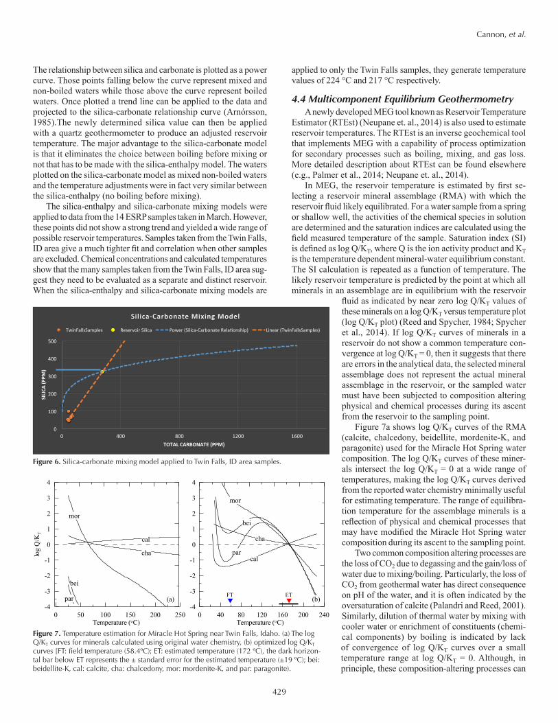
Another mixing model used in adjusting temperature predictions for the possibility for boiling and mixing is the silica-carbonate mixing model (Figure 6). Because, there exists a positive relationship between CO2 concentrations and temperature and the majority of CO2 is in the form of dissolved carbonate, the relationship between total carbonate and silica can be used as a mixing model for thermal waters. The model is particularly useful in separating boiled waters from mixed waters because boiling will result in a drastic reduction in carbonate content while increasing the saturation of silica. Mixing without boiling however, will result in waters with high carbonate/silica ratios.

Table 2. Selected geothermometry temperature values for March ESRP sampling.

Name

Fournier 1977

Fournier and

Potter (1982)

Truesdell (1976)

Fournier (1979)

Giggen-bach

(1988), t>180

Arnorsson (1983) 25-280

Fourner and Truesdell 1973; Fournier, 1977

Qtz (no steam loss)

Qtz (steam loss) Quartz Na-K Na-K-Ca

Na-K-Ca (Mg

Corrected)Heise Hot Springs 85 88 85 221 243 257 227 209 92Lidy Hot Springs 1 89 92 90 477 416 410 457 229 74Lidy Hot Springs 2 85 88 85 466 409 405 448 229 73Green Canyon HS 75 79 76 675 523 501 625 221 69Sturm Well 113 112 113 80 126 146 92 110 110Condie Hot Springs 79 83 80 392 363 364 382 228 95Greenhouse Well 82 85 83 332 323 329 328 195 42Eckert Office Well 104 104 104 101 145 164 112 136 110Campbell Well 1 120 118 120 221 243 256 226 175 109Campbell Well 2 117 116 118 230 250 262 234 177 106Miracle Hot Springs 137 133 137 46 94 115 58 113 113Driscoll Well 98 99 98 24 74 95 36 82 82Driscoll Spring 100 101 100 39 88 109 51 93 93CSI Well 2 114 113 114 96 140 160 107 132 132

Figure 4. Giggenbach ternary diagram of March ESRP thermal samples.

Figure 5. Silica enthalpy mixing model applied to Twin Falls, ID area thermal samples.

429

Cannon, et al.

The relationship between silica and carbonate is plotted as a power curve. Those points falling below the curve represent mixed and non-boiled waters while those above the curve represent boiled waters. Once plotted a trend line can be applied to the data and projected to the silica-carbonate relationship curve (Arnórsson, 1985).The newly determined silica value can then be applied with a quartz geothermometer to produce an adjusted reservoir temperature. The major advantage to the silica-carbonate model is that it eliminates the choice between boiling before mixing or not that has to be made with the silica-enthalpy model. The waters plotted on the silica-carbonate model as mixed non-boiled waters and the temperature adjustments were in fact very similar between the silica-enthalpy (no boiling before mixing).

The silica-enthalpy and silica-carbonate mixing models were applied to data from the 14 ESRP samples taken in March. However, these points did not show a strong trend and yielded a wide range of possible reservoir temperatures. Samples taken from the Twin Falls, ID area give a much tighter fit and correlation when other samples are excluded. Chemical concentrations and calculated temperatures show that the many samples taken from the Twin Falls, ID area sug-gest they need to be evaluated as a separate and distinct reservoir. When the silica-enthalpy and silica-carbonate mixing models are

applied to only the Twin Falls samples, they generate temperature values of 224 °C and 217 °C respectively.

4.4 Multicomponent Equilibrium GeothermometryA newly developed MEG tool known as Reservoir Temperature

Estimator (RTEst) (Neupane et. al., 2014) is also used to estimate reservoir temperatures. The RTEst is an inverse geochemical tool that implements MEG with a capability of process optimization for secondary processes such as boiling, mixing, and gas loss. More detailed description about RTEst can be found elsewhere (e.g., Palmer et al., 2014; Neupane et. al., 2014).

In MEG, the reservoir temperature is estimated by first se-lecting a reservoir mineral assemblage (RMA) with which the reservoir fluid likely equilibrated. For a water sample from a spring or shallow well, the activities of the chemical species in solution are determined and the saturation indices are calculated using the field measured temperature of the sample. Saturation index (SI) is defined as log Q/KT, where Q is the ion activity product and KT is the temperature dependent mineral-water equilibrium constant. The SI calculation is repeated as a function of temperature. The likely reservoir temperature is predicted by the point at which all minerals in an assemblage are in equilibrium with the reservoir

fluid as indicated by near zero log Q/KT values of these minerals on a log Q/KT versus temperature plot (log Q/KT plot) (Reed and Spycher, 1984; Spycher et al., 2014). If log Q/KT curves of minerals in a reservoir do not show a common temperature con-vergence at log Q/KT = 0, then it suggests that there are errors in the analytical data, the selected mineral assemblage does not represent the actual mineral assemblage in the reservoir, or the sampled water must have been subjected to composition altering physical and chemical processes during its ascent from the reservoir to the sampling point.

Figure 7a shows log Q/KT curves of the RMA (calcite, chalcedony, beidellite, mordenite-K, and paragonite) used for the Miracle Hot Spring water composition. The log Q/KT curves of these miner-als intersect the log Q/KT = 0 at a wide range of temperatures, making the log Q/KT curves derived from the reported water chemistry minimally useful for estimating temperature. The range of equilibra-tion temperature for the assemblage minerals is a reflection of physical and chemical processes that may have modified the Miracle Hot Spring water composition during its ascent to the sampling point.

Two common composition altering processes are the loss of CO2 due to degassing and the gain/loss of water due to mixing/boiling. Particularly, the loss of CO2 from geothermal water has direct consequence on pH of the water, and it is often indicated by the oversaturation of calcite (Palandri and Reed, 2001). Similarly, dilution of thermal water by mixing with cooler water or enrichment of constituents (chemi-cal components) by boiling is indicated by lack of convergence of log Q/KT curves over a small temperature range at log Q/KT = 0. Although, in principle, these composition-altering processes can

Figure 6. Silica-carbonate mixing model applied to Twin Falls, ID area samples.

0 50 100 150 200 250Temperature (oC)

-4

-3

-2

-1

0

1

2

3

4

log

Q/K

T

cal

mor

cha

par

0 40 80 120 160 200 240Temperature (oC)

-4

-3

-2

-1

0

1

2

3

4

FT ET

cal

mor

cha

par

(a) (b)

bei

bei

Figure 7. Temperature estimation for Miracle Hot Spring near Twin Falls, Idaho. (a) The log Q/KT curves for minerals calculated using original water chemistry, (b) optimized log Q/KT curves [FT: field temperature (58.4ºC); ET: estimated temperature (172 ºC), the dark horizon-tal bar below ET represents the ± standard error for the estimated temperature (±19 ºC); bei: beidellite-K, cal: calcite, cha: chalcedony, mor: mordenite-K, and par: paragonite).

0  

100  

200  

300  

400  

500  

0   400   800   1200   1600  

SILICA

 (PPM

)  

TOTAL  CARBONATE  (PPM)  

Silica-­‐Carbonate  Mixing  Model  

TwinFallsSamples   Reservoir  Silica   Power  (Silica-­‐Carbonate  Rela�onship)   Linear  (TwinFallsSamples)  

430

Cannon, et al.

be taken into account by simply adding them into the measured water composition and looking for convergence of the saturation indices of the chosen mineral assemblage, a graphical approach becomes cumbersome even for two parameters (e.g., temperature and CO2).

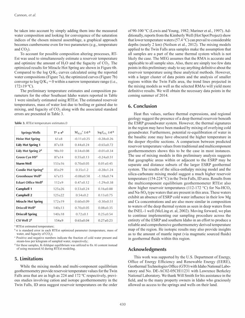
To account for possible composition altering processes, RT-Est was used to simultaneously estimate a reservoir temperature and optimize the amount of H2O and the fugacity of CO2. The optimized results for Miracle Hot Spring are shown in Figure 6b. Compared to the log Q/KT curves calculated using the reported water compositions (Figure 7a), the optimized curves (Figure 7b) converge to log Q/KT = 0 within a narrow temperature range (i.e., 172±19 ºC).

The preliminary temperature estimates and composition pa-rameters for the other Southeast Idaho waters reported in Table 1 were similarly estimated using RTEst. The estimated reservoir temperatures, mass of water lost due to boiling or gained due to mixing, and fugacity of CO2 along with the associated standard errors are presented in Table 3.

5. Limitations

While the mixing models and multi-component equilibrium geothermometry provide reservoir temperature values for the Twin Falls area that are as high as 224 and 172 ºC respectively, previ-ous studies involving cation and isotope geothermometry in the Twin Falls, ID area suggest reservoir temperatures on the order

of 90-100 °C (Lewis and Young, 1982; Mariner et al., 1997). Ad-ditionally, reports from the Kimberly Well (Hot Spot Project) show that lower temperature waters (57.4 °C) can prevail to considerable depths (nearly 2 km) (Neilson et al., 2012). The mixing models applied to the Twin Falls area samples make the assumption that all samples are a part of the same thermal system which is not likely the case. The MEG assumes that the RMA is accurate and applicable to all sample sites. Also, there are simply too few data points in this preliminary study to say anything definitive about the reservoir temperature using these analytical methods. However, with a larger cluster of data points and the analysis of smaller regions within the Twin Falls area, the trend lines projected in the mixing models as well as the selected RMAs will yield more definitive results. We will obtain the necessary data points in the coming summer of 2014.

6. Conclusion

Heat flux values, surface thermal expressions, and regional geology suggest the presence of a deep thermal reservoir beneath the ESRP groundwater system. However, the thermal signatures in the region may have been masked by mixing of overlying cold groundwater. Furthermore, potential re-equilibration of water in the basaltic zone may have obscured the higher temperature in the deeper rhyolite sections. A comparison between predicted reservoir temperature values from traditional and multicomponent geothermometers shows this to be the case in most instances. The use of mixing models in this preliminary analysis suggests that geographic areas within or adjacent to the ESRP may be separate and distance subsets of the larger ESRP geothermal system. The results of the silica-enthalpy mixing model and the silica-carbonate mixing model suggest a much higher reservoir temperature (154-224 °C) in the Twin Falls, ID area. Results from the multicomponent equilibrium geothermometer RTEst also show higher reservoir temperatures (112-172 °C) for Na-HCO3 and Na-SO4 type waters that are present in this area. These waters exhibit an absence of ESRP cold water influence in their low Mg and Ca concentrations and are also more similar in composition to waters of the deep thermal system as seen in deep waters from the INEL-1 well (McLing et. al, 2002). Moving forward, we plan to continue implementing our sampling procedure across the entirety of the ESRP and southern Idaho in an effort to produce a reliable and comprehensive geothermometry derived temperature map of the region. He isotopic results may also provide insights as to the amount of mantle input (via magmatic sourced fluids) in geothermal fluids within this region.

Acknowledgments

This work was supported by the U.S. Department of Energy, Office of Energy Efficiency and Renewable Energy (EERE), Geothermal Technologies Office (GTO) with Idaho National Labo-ratory and No. DE-AC02-05CH11231 with Lawrence Berkeley National Laboratory. We thank Will Smith for his assistance in the field, and to the many property owners in Idaho who graciously allowed us access to the springs and wells on their land.

Table 3. RTEst temperature estimates.0

Springs/Wells Ta ± σb MH2Oc ±σ b log fCO2 ±σ b

Heise Hot Spring 61±8 -0.11±0.25 -0.28±0.26

Lidy Hot Spring 1 87±18 0.44±0.24 -0.65±0.72

Lidy Hot Spring 2d 98±10 0.54±0.08 -0.01±0.34

Green Cyn HSd 87±14 0.55±0.13 -0.24±0.51

Sturm Well 153±16 0.70±0.05 0.01±0.45

Condie Hot Springd 85±29 0.35±1.2 -0.28±1.24

Greenhouse Welld 67±15 -0.08±0.58 -1.18±0.74

Eckart Office Welld 112±9 0.47±0.12 -1.29±0.38

Campbell 1 125±26 0.53±0.24 0.16±0.88

Campbell 2 125±22 0.54±0.2 0.13±0.75

Miracle Hot Spring 172±19 0.60±0.09 -0.30±0.51

Driscoll Welld 140±13 0.70±0.05 0.08±0.35

Driscoll Spring 140±18 0.72±0.1 0.25±0.54

CSI Well 2d 154±9 0.65±0.04 0.27±0.23a RTEst estimated temperature; b σ is standard error in each RTEst optimized parameter (temperature, mass of

water, and fugacity of CO2); c Positive and negative numbers indicate the fraction of cold water present and

steam-loss per kilogram of sampled water, respectively; d for these samples, K-feldspar equilibrium was utilized to fix Al content instead

of using measured Al during RTEst modeling.

431

Cannon, et al.

referencesArnórsson, S., E. Gunnlaugsson, and H. Svavarsson, 1983. “The chemistry of

waters in Iceland.III. Chemical geothermometry in geothermal investiga-tions.” Geochimica Cosmochimica Acta, v. 47, pp. 567-577.

Arnórsson, S., 1985. “The use of mixing models and chemical geothermom-eters for estimating underground temperature in geothermal systems.” J. Volc. Geotherm. Res., v. 23, pp. 299-335.

Bethke, C.M., and S. Yeakel, 2012. “The Geochemist’s Workbench ® Release 9.0 Reaction Modeling Guide.” Aqueous Solutions, LLC, Champaign, Illinois.

Blackwell, D.D., 1989, Regional implications of heat flow of the Snake River Plain, Northwestern United States: Journal of Geophyscial Research, v. 164, p. 323–343.

Blackwell, D.D., and M.C. Richards, 2004. “Geothermal Map of North America.” American Association of Petroleum Geologists, 1 sheet, scale 1:6,500,000.

Brott, C.A., D.D. Blackwell, and J.C. Mitchell, 1976. “Geothermal Inves-tigations in Idaho Part 8: Heat Flow in the Snake River Plain Region, Southern Idaho.” Water Information Bulletin 30, Idaho Department of Water Resources.

Fournier, R.O., and A.H. Truesdell, 1973. “An empirical Na-K-Ca geother-mometer for natural waters.” Geochim. Cosmochim. Acta, v. 37 pp. 1255-1275.

Fournier, R.O., 1977. “Chemical geothermometers and mixing model for geothermal systems.” Geothermics, v. 5, pp. 41-50.

Fournier, R.O., and R.W. Potter, 1979. “Magnesium correction to the Na-K-Ca chemical geothermometer.” Geochim. Cosmochim. Acta v. 43, pp. 1543-1550

Fournier R.O., and R.W. Potter II, 1982. “A revised and expanded silica (quartz) geothermometer.” Geotherm. Resourc. Counc. Bull., v. 11, pp.3-12

Giggenbach, W.F., 1988. “Geothermal solute equilibria. Derivation of Na-K-Mg-Ca geoindicators.” Geochim. Cosmochim. Acta, v. 52, pp. 2749-2765.

Hughes, S.S., R.P. Smith, W.R. Hackett, and S. R. Anderson, 1999. “Mafic volcanism and environmental geology of the eastern Snake River Plain.” Idaho Guidebook to the Geology of Eastern Idaho. Idaho Museum of Natural History, pp. 143-168.

Lewis, R.E., and H.W. Young, 1982. “Geothermal resources in the Banbery Hot Springs Area, Twin Falls County, Idaho.” U.S. Geological Survey Water-Supply Paper 2186, 27 p.

Mariner, R.H., H.W. Young, W.C. Evans, and D.J. Parliman, 1991. “Chemical, isotopic, and dissolved gas compositions of the hydrothermal system in Twin Falls and Jerome Counties, Idaho. Geothermal Resources Council Transactions, v. 15, pp. 257-263.

Mariner, R.H., H.W. Young, T.D. Bullen, and C.J. Janik, 1997. Sulfate-water isotope geothermometery and lead isotope data for regional geothermal system in the Twin Falls area, south-central Idaho. Geothermal Resources Council Transactions, v. 21, pp. 197-201.

McLing, T.L., R.W. Smith, and T.M. Johnson, 2002. “Chemical Characteristics of Thermal Water Beneath the Eastern Snake River Plain Aquifer.” GSA Special Paper 353-13.

Morse, L.H. and McCurry M., 2002. “Genesis of alteration of Quaternary basalts within a portion of the eastern Snake River Plain aquifer.” Special Papers Geological Society of America, 213-224.

Neilson, D.L., C. Delahunty, and J.W. Shervais, 2012. “Geothermal systems in the Snake River Plain, Idaho, Characterized by the Hotspot Project. Geothermal Resources Council Transactions, v. 36, pp.727-730.

Neilson, D.L., and J.W. Shervais, 2014. “Conceptual model for Snake River Plain geothermal systems.” Proceedings, 39th Workshop on Geothermal Reservoir Engineering, Stanford University, Stanford, California, Feb. 24-26, 2014, SGP-TR-202, 7 p.

Neupane, G., E.D. Mattson, T.L. McLing, C.D. Palmer, R.W. Smith, and T.R. Wood, 2014. “Deep geothermal reservoir temperatures in the Eastern Snake River Plain, Idaho using multicomponent geothermometry.” Proceedings, 39th Workshop on Geothermal Reservoir Engineering, Stanford University, Stanford, California, February 24-26, 2014 SGP-TR-202, 12 p.

Palandri, J.L., and M.H. Reed, 2001. “Reconstruction of in situ composition of sedimentary formation waters.” Geochimica et Cosmochimica Acta, v. 65, pp. 1741-1767.

Palmer, C.D., S.R. Ohly, R.W. Smith, G. Neupane, T. McLing, and E. Mattson, 2014. “Mineral Selection for Multicomponent Equilibrium Geother-mometry.” Geothermal Resources Council Transactions, this volume.

Pang, Z.H., and M. Reed, 1998. “Theoretical chemical thermometry on geo-thermal waters: Problems and methods.” Geochimica et Cosmochimica Acta, v. 62, pp. 1083-1091.

Parliman, D.J., and H.W. Young, 1992. “Compilation of selected data for thermal-water wells and springs in Idaho, 1921 through 1991.” U.S. Geological Survey Open-File Report 92-175, 201 p.

Pierce, K.L., and L.A. Morgan, 1992. “The track of the Yellowstone hot spot--volcanism, faulting and uplift.” In: Link, P.K., M.A. Kuntz, and L.W. Platt, eds., Regional geology of eastern Idaho and western Wyoming. Geological Society of America Memoir 179, pp. 1-53.

Ralston, D.R., J.L. Arrigo, J.V. Baglio Jr., L.M. Coleman, K. Souder, and A.L. Mayo, 1981. “Geothermal evaluation of the thrust area zone in southeastern Idaho.” Idaho Water and Energy Research Institute, Uni-versity of Idaho, 110 p.

Reed, M., and N. Spycher, 1984. “Calculation of pH and mineral equilibria in hydrothermal waters with application to geothermometry and studies of boiling and dilution.” Geochimica et Cosmochimica Acta, v. 48, pp. 1479-1492.

Rodgers, D.W., H.T. Ore, R.T. Bobo, N. McQuarrie, and N. Zentner, 2002. “Extension and subsidence of the eastern Snake River Plain, Idaho.” In: C.M. White and M. McCurry, eds., Tectonic and Magmatic Evolution of the Snake River Plain Province: Idaho Geologic Survey Bulletin 30, pp. 121-155.

Ross, S.H., 1971. “Geothermal potential of Idaho.” Idaho Bureau of Mines and Geology, Pamphlet 150, 72 p.

Shervais, J.W., D.R. Schmitt, D. Nielson, J.P. Evans, E.H. Christainsen, L. Morgan, W.C. Shanks, A. A. Prokopenko, T. Lachmar, L.M. Liberty, D.D. Blackwell, J.M. Glen, D. Champion, K.E. Potter, J.A. Kessler, 2013. “First results from HOTSPOT: The Snake River Plain Scientific Drilling Project, Idaho, U.S.A.” Scientific Drilling, n. 15, pp. 36-45.

Smith, R.P., 2004. “Geologic setting of the Snake River Plain aquifer and vadose zone.” Vadose Zone Journal, v. 3, pp. 47-58.

Spycher, N., L. Peiffer, E.L. Sonnenthal, M.H. Reed, and B.M. Kennedy, 2014. “Integrated multicomponent solute geothermometry.” Geothermics, v. 51, pp. 113-123.

Truesdell, A.H., 1976. “Summary of section III - geochemical techniques in exploration.” Proceedings of the 2nd U.N. Symposium on the Develop-ment and Use of Geothermal Resources, San Francisco, v. 1, liii-lxxix.

Whitehead, R.L., 1992. “Geohydrologic Framework of the Snake River Plain Regional Aquifer System, Idaho and Eastern Oregon.” U.S. Geological Survey Professional Paper 1408-B, pp. 7-22.

Wood, W.W., and W.H. Low, 1988. “Solute chemistry of the Snake River Plain Regional Aquifer System, Idaho and Eastern Oregon.” U.S. Geological Survey Professional Paper 1408-D, 79 p.

Young, H.W., and J.C. Mitchell, 1973. “Geothermal Investigations in Idaho Part 1: Geochemistry and Geologic Setting of Selected Thermal Waters.” USGS, IDWR Water Information Bulletin No. 30, pp. 23-28.

432