Embed Size (px)
Citation preview
8/3/2019 Genta Kawahara et al- Wrap, tilt and stretch of vorticity lines around a strong thin straight vortex tube in a simple …
http://slidepdf.com/reader/full/genta-kawahara-et-al-wrap-tilt-and-stretch-of-vorticity-lines-around-a-strong 1/49
Engineering
Mechanical Engineering fields
Okayama University Year 1997
Wrap, tilt and stretch of vorticity lines
around a strong thin straight vortex tube
in a simple shear flowGenta Kawahara∗ Shigeo Kida†
Mitsuru Tanaka‡ Shinichiro Yanase∗∗
∗Ehime University†National Institute for Fusion Science
‡Kyoto Institute of Technology∗∗Okayama University
This paper is posted at eScholarship@OUDIR : Okayama University Digital InformationRepository.
http://escholarship.lib.okayama-u.ac.jp/mechanical engineering/32
8/3/2019 Genta Kawahara et al- Wrap, tilt and stretch of vorticity lines around a strong thin straight vortex tube in a simple …
http://slidepdf.com/reader/full/genta-kawahara-et-al-wrap-tilt-and-stretch-of-vorticity-lines-around-a-strong 2/49
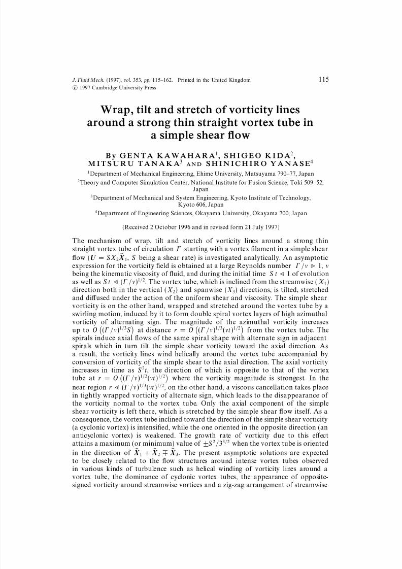
J. Fluid Mech. (1997), vol. 353, pp. 115–162. Printed in the United Kingdom
c 1997 Cambridge University Press
115
Wrap, tilt and stretch of vorticity linesaround a strong thin straight vortex tube in
a simple shear flow
B y G E N T A K A W A H A R A1, S H I G E O K I D A2,M I T S U R U T A N A K A3
A N D S H I N I C H I R O Y A N A S E4
1Department of Mechanical Engineering, Ehime University, Matsuyama 790–77, Japan2Theory and Computer Simulation Center, National Institute for Fusion Science, Toki 509–52,
Japan3
Department of Mechanical and System Engineering, Kyoto Institute of Technology,Kyoto 606, Japan4Department of Engineering Sciences, Okayama University, Okayama 700, Japan
(Received 2 October 1996 and in revised form 21 July 1997)
The mechanism of wrap, tilt and stretch of vorticity lines around a strong thinstraight vortex tube of circulation Γ starting with a vortex filament in a simple shear
flow (U = SX 2 X 1, S being a shear rate) is investigated analytically. An asymptoticexpression for the vorticity field is obtained at a large Reynolds number Γ /ν 1, νbeing the kinematic viscosity of fluid, and during the initial time S t 1 of evolutionas well as S t (Γ /ν)1/2. The vortex tube, which is inclined from the streamwise (X 1)direction both in the vertical (X 2) and spanwise (X 3) directions, is tilted, stretched
and diffused under the action of the uniform shear and viscosity. The simple shearvorticity is on the other hand, wrapped and stretched around the vortex tube by aswirling motion, induced by it to form double spiral vortex layers of high azimuthalvorticity of alternating sign. The magnitude of the azimuthal vorticity increasesup to O
(Γ /ν)1/3S
at distance r = O
(Γ /ν)1/3(νt)1/2
from the vortex tube. The
spirals induce axial flows of the same spiral shape with alternate sign in adjacentspirals which in turn tilt the simple shear vorticity toward the axial direction. Asa result, the vorticity lines wind helically around the vortex tube accompanied byconversion of vorticity of the simple shear to the axial direction. The axial vorticityincreases in time as S 2t, the direction of which is opposite to that of the vortextube at r = O
(Γ /ν)1/2(νt)1/2
where the vorticity magnitude is strongest. In the
near region r (Γ /ν)1/3(νt)1/2, on the other hand, a viscous cancellation takes place
in tightly wrapped vorticity of alternate sign, which leads to the disappearance of the vorticity normal to the vortex tube. Only the axial component of the simpleshear vorticity is left there, which is stretched by the simple shear flow itself. As aconsequence, the vortex tube inclined toward the direction of the simple shear vorticity(a cyclonic vortex) is intensified, while the one oriented in the opposite direction (ananticyclonic vortex) is weakened. The growth rate of vorticity due to this effectattains a maximum (or minimum) value of ±S 2/33/2 when the vortex tube is oriented
in the direction of X 1 + X 2 X 3. The present asymptotic solutions are expectedto be closely related to the flow structures around intense vortex tubes observedin various kinds of turbulence such as helical winding of vorticity lines around avortex tube, the dominance of cyclonic vortex tubes, the appearance of opposite-signed vorticity around streamwise vortices and a zig-zag arrangement of streamwise
8/3/2019 Genta Kawahara et al- Wrap, tilt and stretch of vorticity lines around a strong thin straight vortex tube in a simple …
http://slidepdf.com/reader/full/genta-kawahara-et-al-wrap-tilt-and-stretch-of-vorticity-lines-around-a-strong 3/49
116 G. Kawahara, S. Kida, M. Tanaka and S. Yanase
vortices in homogeneous isotropic turbulence, homogeneous shear turbulence and
near-wall turbulence.
1. Introduction
Tube-like vortical structures of concentrated high vorticity have been commonlyobserved in many turbulent flow fields. In homogeneous isotropic turbulence, thereexist strong coherent elongated vortices in a weaker background vorticity, and arelatively large portion of turbulence kinetic energy is dissipated around them (Siggia1981; Kerr 1985; Hosokawa & Yamamoto 1989; She, Jackson & Orszag 1990;Ruetsch & Maxey 1991; Vincent & Meneguzzi 1991; Douady, Couder & Brachet1991; Kida & Ohkitani 1992; Jimenez et al. 1993; Kida 1993). In homogeneous shearturbulence, Kida & Tanaka (1992, 1994) showed the presence of longitudinal vortextubes which induce an intense Reynolds shear stress, and clarified their generation anddevelopment processes. In near-wall turbulence, it was found that streamwise vortextubes play a central role in the production of turbulence kinetic energy (Robinson,Kline & Spalart 1988; Brooke & Hanratty 1993; Bernard, Thomas & Handler 1993).In near-wall turbulence streamwise vortices are closely related to the generation of high skin friction (Choi, Moin & Kim 1993; Kravchenko, Choi & Moin 1993).Another example of tube-like concentrated vortices is the ribs observed in a turbulentmixing layer (see Hussain 1986). These observations lead us to believe that tube-like vortices may be one of the key ingredients of coherent structures which make asignificant contribution to the production and dissipation of turbulence kinetic energy.They are also expected to control heat, mass and momentum transfers. Clarification
of the dynamics of vortex tubes would lead to a new concept useful for understandingand controlling turbulence phenomena.
In the time evolution of tube-like structures their interactions with a backgroundturbulence field are considered to play a significant role. It is understood at leastconceptually that a background turbulence stretches and rotates vortex tubes as wellas deforms their shape and that the vortex tubes, on the other hand, wrap andstretch the background vorticity lines. We must admit, however, that the knowledgeof the actual dynamical process in these interactions is still poor. There has beenmuch effort devoted to this subject. Moore (1985) investigated the dynamics of adiffusing straight vortex tube perfectly aligned with a simple shear flow. He derived alarge-Reynolds-number asymptotic solution to show that excessive vorticity wrappingenhances viscous cancellation to expell the shear flow vorticity near the vortex tube.
In their asymptotic analysis of a strong vortex tube subjected to a uniform non-axisymmetric irrotational strain, Moffatt, Kida & Ohkitani (1994) found that at largeReynolds numbers, a stretched vortex tube can survive for a long time even when twoof the principal rates of strain are positive. Recently, Jimenez, Moffatt & Vasco (1996)applied Moffatt et al. (1994) asymptotic theory to the dynamics of a two-dimensionaldiffusing vortex tube in an imposed weak strain. They showed a good agreementbetween the results of their theory and a numerical simulation of two-dimensionalturbulence.
In this paper, we study vorticity dynamics, especially vortex wrapping, tilting andstretching, around a strong thin straight vortex tube starting with a vortex filament
in a simple shear flow (U = SX 2 X 1, S being a shear rate). A straight vortex filamentof circulation Γ is set at an initial instant, being inclined away from the streamwise
8/3/2019 Genta Kawahara et al- Wrap, tilt and stretch of vorticity lines around a strong thin straight vortex tube in a simple …
http://slidepdf.com/reader/full/genta-kawahara-et-al-wrap-tilt-and-stretch-of-vorticity-lines-around-a-strong 4/49
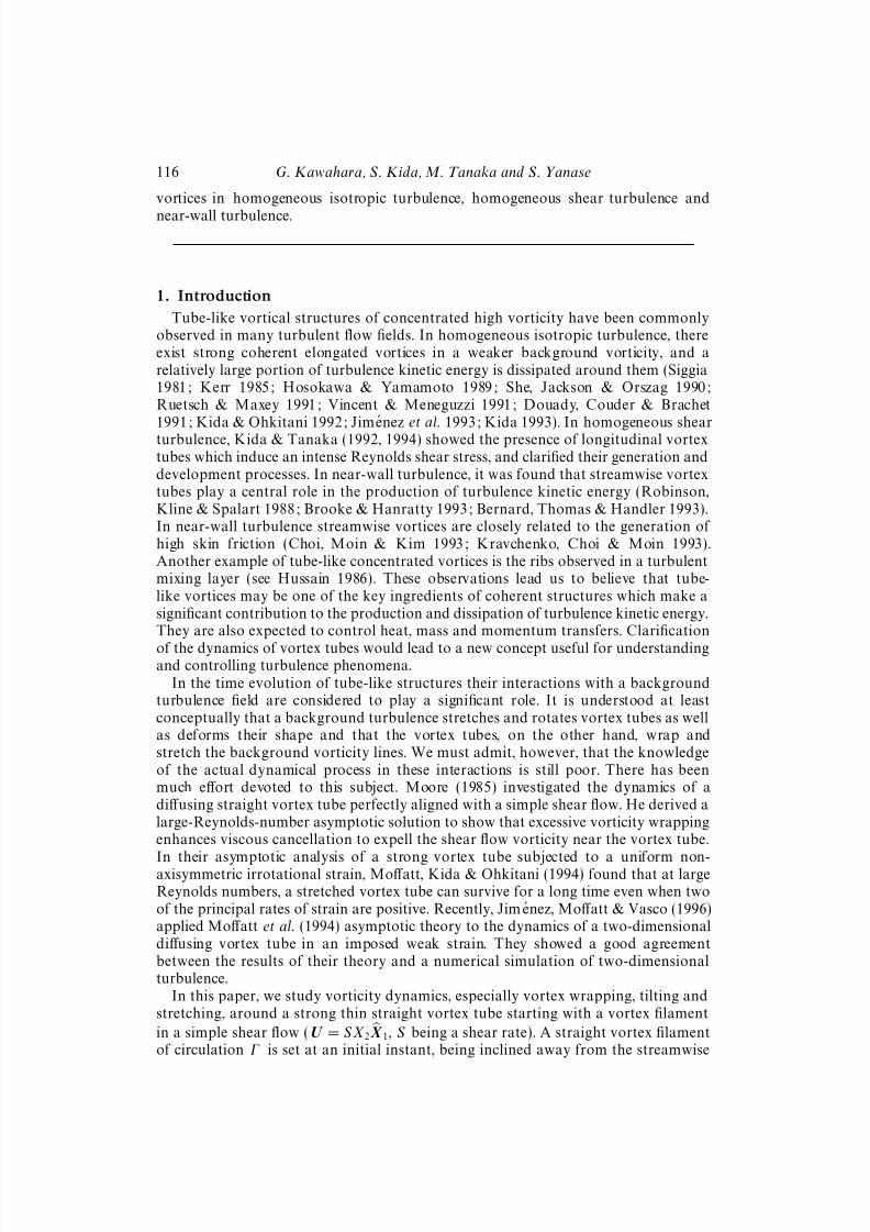
Wrap, tilt and stretch of vorticity lines 117
X 2
X 1
X 3
O
] × U
= – S X
ˆ 3U = S X 2 X ˆ1
Figure 1. A straight vortex tube in a simple shear flow.
(X 1) direction both in the vertical (X 2) and spanwise (X 3) directions. The vortexfilament is tilted, stretched and diffused under the action of the uniform shear andviscosity. The strength of a vortex tube may be measured by the vortex Reynoldsnumber Γ /ν, where ν is the kinematic viscosity of fluid. We are particularly interestedin a strong vortex tube (Γ /ν 1) since the vortex Reynolds number often takeslarge values in typical turbulence. For example, Robinson (1991) observed Γ /ν ≈140 in boundary-layer turbulence at momentum-thickness Reynolds number Reθ =670, while Jimenez et al. (1993) found that in homogeneous isotropic turbulence
Γ /ν increases with Taylor-microscale Reynolds number Reλ as Γ /ν ∼ Re
1/2
λ . Anasymptotic analysis is performed at a large Reynolds number Γ /ν 1 and at theinitial time S t 1 of evolution. The problem to be considered here includes the onestreated by Moore (1985) and by Jimenez et al. (1996) as special cases.
In §2, we derive the equations of motion of a vortex tube in a simple shear flowin a coordinate system rotating with the central axis of the vortex tube under theassumption that the vorticity and induced velocity of the vortex tube are uniformalong its axis. Asymptotic solutions starting with a vortex filament are presented forΓ /ν 1 and S t 1 by extending Moore’s (1985) and Moffatt et al.’s (1994) methodsin §3 (details of the analysis for higher orders are described in Appendices A andB). In §4, we provide a physical interpretation of the asymptotic solutions to explorestructures of the vorticity field. Section 5 is devoted to concluding remarks.
2. Formulation
We consider the motion of a straight vortex tube in a simple shear flow withuniform pressure P (see figure 1). Let the coordinate system OX 1X 2X 3 be at rest, theX 1-axis being aligned with the shear flow direction. The uniform shear velocity U is
taken to depend only on X 2, i.e. U = S X 2 X 1, where S (> 0) denotes the shear rate,
which is constant in time, and X i is the unit vector in the X i-direction (i = 1, 2, 3).
In this configuration the uniform shear vorticity is given by × U = −S X 3, whichis anti-parallel to the X 3-axis. Hereafter, we call X 1, X 2 and X 3 the streamwise, thevertical and the spanwise coordinates, respectively.
The vortex tube is inclined both vertically and horizontally away from the stream-
8/3/2019 Genta Kawahara et al- Wrap, tilt and stretch of vorticity lines around a strong thin straight vortex tube in a simple …
http://slidepdf.com/reader/full/genta-kawahara-et-al-wrap-tilt-and-stretch-of-vorticity-lines-around-a-strong 5/49
118 G. Kawahara, S. Kida, M. Tanaka and S. Yanase
X 1
x3
X 3
x2
X 2
x1
αβ
β α
β
α
O
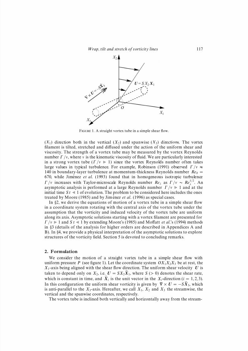
Figure 2. Structural coordinate system Ox1x2x3
and the original stationary coordinate system OX 1X 2X 3.
wise direction. It will be tilted and stretched by the uniform shear. The origin O islocated on the central axis of the vortex tube, so that it is a stagnation point of the flow. We suppose that the vortex tube is of infinite extent, and its vorticity andinduced velocity are uniform along its axis.
2.1. Structural coordinate system
We formulate the problem in a rotating coordinate system Ox1x2x3 as shown infigure 2. Rotating the stationary coordinate system OX 1X 2X 3 by an angle β aroundthe X 1-axis, we set the new X 3-direction as the x3-axis. Next, we further rotateOX 1X 2X 3 by an angle α around the x3-axis (new X 3-axis), and then the new X 1- andX 2-directions are set as the x1- and x2-coordinates, respectively. Rotation angles, αand β, are taken so that the resulting x1-axis may coincide with the central axis of the vortex tube. The vorticity of the vortex tube is taken to be pointed in the positivex1-direction. Hereafter, we call Ox1x2x3 the structural coordinate system, x1 the axialcoordinate and (x2, x3) the normal plane. Flow symmetry allows us to take α and βin the range 0 6 α < π and − 1
2π 6 β 6 1
2π without loss of generality. In the case
of α = 0, the vortex tube is aligned with the streamwise direction. When α < (or >)12
π, it is inclined downstream (or upstream). In the cases of β = ± 12
π, the tube axis
is located on the horizontal plane X 2 = 0. When β < (or >) 0, the spanwise vorticitycomponent of the vortex tube is negative (or positive). Hereafter, a vortex tube forβ < (or >) 0 is referred to as a cyclonic (or anticyclonic) vortex.
Two vectors, (V 1, V 2, V 3) in OX 1X 2X 3 and (v1, v2, v3) in Ox1x2x3, are connected bythe relation
V i = M ij vj (i = 1, 2, 3), (2.1)
where
M ij =
cos α − sin α 0sin α cos β cos α cos β − sin βsin α sin β cos α sin β cos β
(i, j = 1, 2, 3) (2.2)
is a transformation matrix which represents a system rotation. Here and subsequently,
8/3/2019 Genta Kawahara et al- Wrap, tilt and stretch of vorticity lines around a strong thin straight vortex tube in a simple …
http://slidepdf.com/reader/full/genta-kawahara-et-al-wrap-tilt-and-stretch-of-vorticity-lines-around-a-strong 6/49
Wrap, tilt and stretch of vorticity lines 119
the summation convention is employed for repeated subscripts. Similarly, the unit
vectors representing the axes in the two coordinate systems are related by X i = M ij xj (i = 1, 2, 3). (2.3)
As the vortex tube evolves, the structural coordinate system Ox1x2x3 rotates aroundsome axis which passes through the origin O. It follows from the definition of α andβ that the angular velocity of the system rotation Ω is given by
Ω = (dtβ) X 1 + (dtα) x3, (2.4)
where dt ≡ d/dt. By making use of (2.2) and (2.3), we can express each componentof the angular velocity vector in Ox1x2x3 as
Ω1 = (dtβ)cos α, Ω2 = −(dtβ)sin α, Ω3 = dtα. (2.5a–c)
2.2. Angular velocity of structural coordinate system
The motion of an incompressible viscous fluid of uniform mass density (taken as unity)is described by the Navier–Stokes equation, or equivalently the vorticity equation,which are respectively written in the structural coordinate system Ox1x2x3 as †
∂tu + [(u−Ω× x) · ]u = u×Ω− p + ν2u, (2.6)
∂tω + [(u−Ω× x) · ]ω = ω ×Ω + (ω · )u + ν2ω, (2.7)
where u(x1, x2, x3, t) is the velocity field relative to the stationary coordinate system,ω = × u is the vorticity, p is the pressure and is the gradient operator in thestructural coordinate system. The continuity equation is written as
· u = 0. (2.8)
Now let us decompose the velocity, the vorticity and the pressure fields intocontributions from the simple shear flow and the fluctuation field as
u = U + u, ω = ×U + ω
, p = P + p. (2.9)
Then, the time evolutions of the fluctuation velocity and vorticity are described by
∂tu + [(u + u) · ]u = u
×Ω− (u· )U − p + ν2
u, (2.10)
∂tω + [(u + u) · ]ω = ω
×Ω + (ω· )U + [(ω + ×U ) · ]u + ν2
ω, (2.11)
· u = 0, (2.12)
ω = × u
, (2.13)
whereu = U −Ω× x (2.14)
is the simple shear velocity relative to the structural coordinate system. The simpleshear velocity and vorticity are respectively written as
U = SX 2 X 1 = SM 1iM 2j xj xi, (2.15)
×U = −S X 3 = −S M 3i xi. (2.16)
Notice that in general the coordinate x1 appears explicitly in u2 and u3. If we
† Recall that a time derivative of a vector field A in a stationary coordinate system is replacedby ∂tA → ∂tA− [(Ω× x) · ]A + Ω× A in the structural coordinate system.

8/3/2019 Genta Kawahara et al- Wrap, tilt and stretch of vorticity lines around a strong thin straight vortex tube in a simple …
http://slidepdf.com/reader/full/genta-kawahara-et-al-wrap-tilt-and-stretch-of-vorticity-lines-around-a-strong 7/49
120 G. Kawahara, S. Kida, M. Tanaka and S. Yanase
X 1
X 3
X 2
β
O
cot α0 St cos β
cot α(t )
α(t )
α0
1
c o s β
Figure 3. Movement of a vortex tube (i.e. the x1-axis) which is shown by a white-head arrow.
require, however, that u and ω are uniform in the x1-direction, it follows from (2.10)
and (2.11) that u2 and u3 are independent of x1. Then we have
Ω2 = 0, Ω3 = −S sin2 α cos β. (2.17)
Equations (2.5b,c) then give
(dtβ)sin α = 0, (2.18)
dtα =
−S sin2 α cos β. (2.19)
Equations (2.18) and (2.19) have a trivial solution α ≡ 0 for any arbitrary β. Exceptfor this trivial case, (2.18) requires that
dtβ = 0. (2.20)
In the case of α ≡ 0, the vortex axis (x1-axis) is identical with the X 1-axis, and anyrotation around this axis does not change the orientation of it, so that we can takeβ to be constant in time t. Hence, we can assume that β is constant in any case.Equation (2.5a) then yields
Ω1 = 0. (2.21)
Equations (2.17) and (2.21) tell us that Ω has only the x3-component. By integrating
(2.19), we obtaincot α = cot α0 + S t cos β (2.22)
with α0 denoting the initial value of α at t = 0. It follows from (2.22) that α → 0 asα0 → 0. Thus, the trivial solution (α ≡ 0) is included in (2.22). These considerationslead us to the conclusion that a vortex tube rotates on a plane inclined to the spanwisedirection at an angle of β which is invariant in time, and angle α from the streamwisedirection approaches zero according to (2.22) as time progresses. This implies that thecentral axis of the vortex tube, the velocity and vorticity of which are uniform alongit, must be passively convected by the uniform shear flow (see figure 3). Note that inthe special cases of α = 0 or β = ± 1
2π, the vortex tube is not inclined vertically and
is stationary.
8/3/2019 Genta Kawahara et al- Wrap, tilt and stretch of vorticity lines around a strong thin straight vortex tube in a simple …
http://slidepdf.com/reader/full/genta-kawahara-et-al-wrap-tilt-and-stretch-of-vorticity-lines-around-a-strong 8/49
Wrap, tilt and stretch of vorticity lines 121
2.3. Basic equations
Suppose now that the fluctuation fields ω, u and p are independent of x1, i.e. ∂1 = 0.We then obtain closed equations for ω
1 and u1 from (2.10) and (2.11) as
∂tω1 − ∂(ψ, ω
1)
∂(x2, x3)− S (γ(t)x2 + λ(t)x3)∂2ω
1 = Sγ(t)ω1 + S ξ(t)∂3u
1 + ν2⊥ω
1, (2.23)
∂tu1 − ∂(ψ, u
1)
∂(x2, x3)− S (γ(t)x2 + λ(t)x3)∂2u
1
= −Sγ(t)u1 − S (cos α sin β ∂2 + cos β ∂3)ψ + ν2
⊥u1, (2.24)
where ψ (u2 = ∂3ψ, u
3 = −∂2ψ) is the streamfunction, which is related to ω1 via
2
⊥ψ =
−ω
1, (2.25)
and
γ(t) =∂1U1
S = cos α sin α cos β, (2.26)
λ(t) =( ×U ) · x1
S = − sin α sin β, (2.27)
ξ(t) =2Ω3
S = −2sin2 α cos β (6 0) (2.28)
(cf. (2.15)–(2.17)). Here, 2⊥ = ∂22 + ∂2
3 is a two-dimensional Laplacian operator. Notethat γ(t) represents the axial rate of strain of the simple shear flow, λ(t) the axialcomponent of the simple shear vorticity, and ξ(t) the vorticity corresponding to theangular velocity of the structural coordinate system, all of which are normalized bythe simple shear rate. Note also that the nonlinear stretching-and-tilting terms ω
j ∂j u1
have disappeared from (2.23) because the flow field is uniform along the vortex tube.Once (2.23) and (2.24) are solved, we can calculate the other two fluctuation vorticitycomponents through
ω2 = ∂3u
1, ω3 = −∂2u
1. (2.29)
The second and third terms on the left-hand sides of (2.23) and (2.24) represent theadvection by the fluctuation velocity and the simple shear, respectively. On the right-hand side of (2.23), the first term represents the vorticity stretching via the simpleshear, while the second is the production of the axial (x1) component of the fluctuationvorticity via the tilting by the velocity fluctuation of the vorticity associated with thesystem rotation which has only an x3-component. This second term is also interpreted
as a sum of three contributions: the tilting of the x2-component of the fluctuationvorticity through the simple shear, ω2∂2U1 = S cos2 α cos β ∂3u
1; the tilting of thex3-component of the simple shear vorticity via the velocity fluctuation, −SM 33∂3u
1 =
−S cos β ∂3u1; and the effect of frame rotation, (ω ×Ω) · x1 = −S sin2 α cos β ∂3u
1. If β = ± 1
2π, all of these three contributions vanish. If α = 0, the tiltings of the fluctuation
vorticity and the simple shear vorticity cancel out, and the effect of frame rotationvanishes. Thus, in these two special cases, the production term on the right-handside of (2.23) disappears. Except for these cases, the effect of the tilting of the simpleshear vorticity is important in production of the axial vorticity. Note that this termis negative (or positive) according as ω
2 = ∂3u1 > (or <) 0. On the right-hand side
of (2.24), the first two terms originate from the advection of the simple shear velocityby the velocity fluctuation and the frame rotation.
8/3/2019 Genta Kawahara et al- Wrap, tilt and stretch of vorticity lines around a strong thin straight vortex tube in a simple …
http://slidepdf.com/reader/full/genta-kawahara-et-al-wrap-tilt-and-stretch-of-vorticity-lines-around-a-strong 9/49
122 G. Kawahara, S. Kida, M. Tanaka and S. Yanase
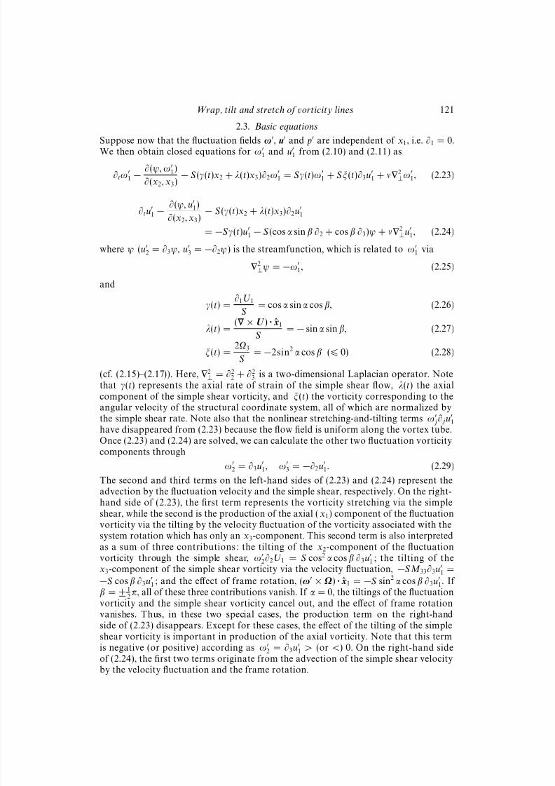
0 1 2 3 4 5
1
2
3
4
St
A(t )
β = 0
β =1
4p
β =1
2p
Figure 4. Time-variation of stretch factor A(t) for α0 = 14
π and for three values of β.
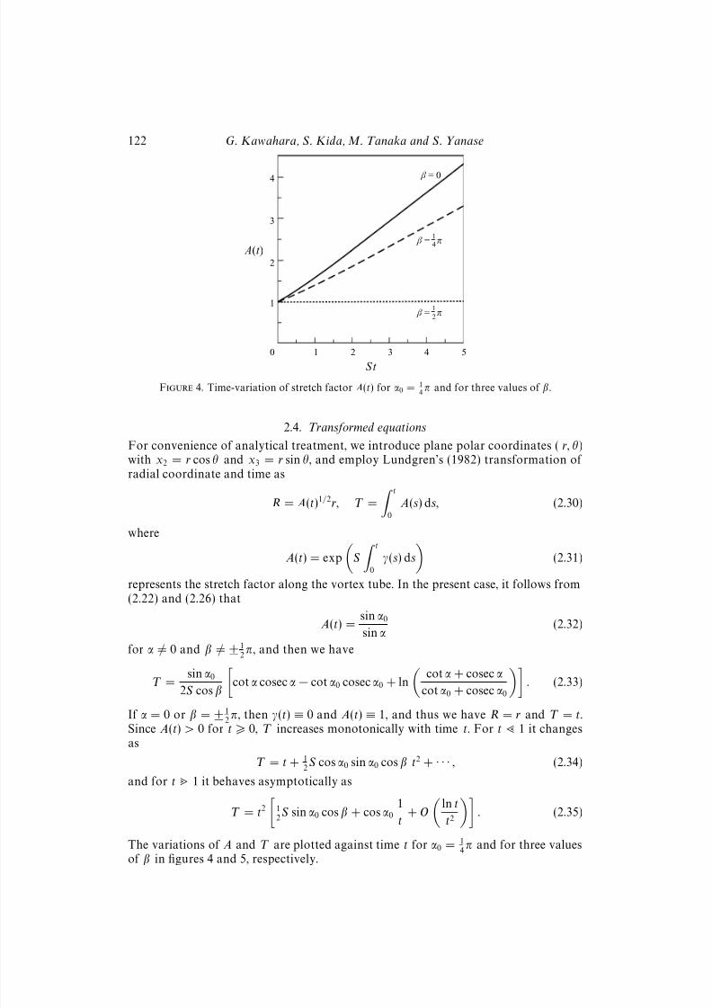
2.4. Transformed equations
For convenience of analytical treatment, we introduce plane polar coordinates ( r, θ)with x2 = r cos θ and x3 = r sin θ, and employ Lundgren’s (1982) transformation of radial coordinate and time as
R = A(t)1/2r, T =
t
0
A(s) ds, (2.30)
where
A(t) = exp
S
t
0
γ(s) ds
(2.31)
represents the stretch factor along the vortex tube. In the present case, it follows from(2.22) and (2.26) that
A(t) =sin α0
sin α(2.32)
for α = 0 and β = ± 12
π, and then we have
T =sin α0
2S cos β
cot α cosec α − cot α0 cosec α0 + ln
cot α + cosec α
cot α0 + cosec α0
. (2.33)
If α = 0 or β = ± 12
π, then γ(t) ≡ 0 and A(t) ≡ 1, and thus we have R = r and T = t.Since A(t) > 0 for t > 0, T increases monotonically with time t. For t 1 it changesas
T = t + 12
S cos α0 sin α0 cos β t2 + · · · , (2.34)
and for t 1 it behaves asymptotically as
T = t2
12
S sin α0 cos β + cos α0
1
t+ O
ln t
t2
. (2.35)
The variations of A and T are plotted against time t for α0 = 14
π and for three valuesof β in figures 4 and 5, respectively.
8/3/2019 Genta Kawahara et al- Wrap, tilt and stretch of vorticity lines around a strong thin straight vortex tube in a simple …
http://slidepdf.com/reader/full/genta-kawahara-et-al-wrap-tilt-and-stretch-of-vorticity-lines-around-a-strong 10/49
Wrap, tilt and stretch of vorticity lines 123
0 1 2 3 4 5
5
10
St
ST (t )
β = 0
β =1
4p
β =1
2p
Figure 5. Time-variation of modified time T (t) for α0 = 14
π and for three values of β.
Equation (2.24) has a particular solution
u1p = −S cos β x2 + S cos α sin β x3(≡ −Sr Re[i f∞(t)e−iθ], say), (2.36)
which will turn out to play a key role in vorticity dynamics near the vortex core (see§3.4), where
f∞(t) = − cos α sin β − icos β = −D(t)eiϕ(t) (2.37)
with
D(t) = (cos2 α sin2 β + cos2 β)1/2, ϕ(t) = arctan
cos β
cos α sin β
(0 6 ϕ(t) 6 π). (2.38)
Note that ∂3u1p = S cos α sin β = SM 32 and −∂2u
1p = S cos β = SM 33, i.e. the vorticityassociated with this particular solution is equal to minus the component normal tothe vortex tube of the simple shear vorticity. If we introduce a new dependent variableu
1 by
u1 = u
1p + u1 (2.39)
and substitute it into (2.24), we can eliminate the inhomogeneous term on the right-hand side of (2.24). Then, ∂3u
1 and −∂2u1 are equal to the x2- and x3-components of
the total vorticity, respectively, i.e. ω2 = ∂3u1 and ω3 =
−∂2u
1 .
Equations (2.23) and (2.24) are now transformed into closed equations for newdependent variables†
ω(R ,θ ,T ) = ω1(r ,θ ,t)/A(t) = −2
Rψ, R u(R ,θ ,T ) = A(t)u1(r ,θ ,t) (2.40)
as
− 1
R
∂(ψ, ω)
∂(R, θ)+ (∂T − ν2
R)ω = SL1ω + SL2u +2S 2γ(t)λ(t)
A(t)2, (2.41)
− 1
R
∂(ψ,Ru)
∂(R, θ)+ (∂T − ν2
R)Ru = SL1Ru, (2.42)
† Notice that the axial velocity is expressed by R u not by u.
8/3/2019 Genta Kawahara et al- Wrap, tilt and stretch of vorticity lines around a strong thin straight vortex tube in a simple …
http://slidepdf.com/reader/full/genta-kawahara-et-al-wrap-tilt-and-stretch-of-vorticity-lines-around-a-strong 11/49
124 G. Kawahara, S. Kida, M. Tanaka and S. Yanase
where
2R = ∂2
R + 1R
∂R + 1R2
∂2θ (2.43)
is the two-dimensional Laplacian operator, and
L1 =1
2 A(t)[γ(t)(− sin2θ ∂θ + R cos2θ ∂R) + λ(t)(cos 2θ ∂θ + R sin2θ ∂R − ∂θ)], (2.44)
L2 =ξ(t)
A(t)5/2[cos θ ∂θ + sin θ (R∂R + 1)] (2.45)
are first-order differential operators. The components of the total vorticity are ex-pressed in terms of ω and u as
ω1 = S λ(t) + A(t)ω, (2.46)
ω2 = A(t)−1/2[cos θ ∂θ + sin θ (R∂R + 1)]u, (2.47)
ω3 = A(t)−1/2[sin θ ∂θ − cos θ (R∂R + 1)]u. (2.48)
The right-hand sides of (2.41) and (2.42) represent the effects of the simple shear onthe fluctuation fields. The first terms, S L1ω and SL1Ru, represent respectively thedeformation of the spatial distribution of ω and u in the normal (x2, x3)-plane bythe simple shear. The last two terms on the right-hand side of (2.41) represent thecoupling effect of the axial vorticity and velocity, that is, the second term on theright-hand side of (2.23), which is composed of the tilting of the x2-component of thefluctuation vorticity by the simple shear, the tilting of the x3-component of the simpleshear vorticity via the velocity fluctuation, and the effect of the frame rotation. Thelast term is the contribution from particular solution (2.36). Note that if a vortex tube
was not inclined vertically (α = 0 or β = ±12 π), the second and third terms would
vanish, so that ω would be decoupled from u. In these special cases the problem ismuch simplified. Pearson & Abernathy (1984) and Moore (1985) studied the timeevolution of a diffusing vortex tube perfectly aligned with a simple shear (α = 0), andrecently Jimenez et al. (1996) examined the structure of a two-dimensional diffusingvortex tube in an imposed weak strain (α = 1
2π and β = ± 1
2π). The present analysis
includes both of them.
3. Asymptotic analysis at Re 1 and ST 1
In this section, we consider an early stage of time evolution of a strong thin straightvortex tube starting with a vortex filament. A straight vortex filament with circulationΓ is put in a simple shear flow at an initial instant T = 0. That is, the fluctuationvorticity is concentrated on a straight line R = 0, i.e.
ω|T =0 =Γ δ(R)
πR, (3.1)
and the fluctuation axial velocity along the filament is null, u1 = 0, so that, from
(2.36)–(2.40),
u|T =0 = S Re[i f0e−iθ], (3.2)
where
f0 = − cos α0 sin β − icos β = −D0eiϕ0 (3.3)

8/3/2019 Genta Kawahara et al- Wrap, tilt and stretch of vorticity lines around a strong thin straight vortex tube in a simple …
http://slidepdf.com/reader/full/genta-kawahara-et-al-wrap-tilt-and-stretch-of-vorticity-lines-around-a-strong 12/49
Wrap, tilt and stretch of vorticity lines 125
Variables T R ω ψ R u
Units 1/S (ν/S )1/2 −1S (= ΓS/ν) −1ν (= Γ ) (νS )1/2
Table 1. Units for variables
with
D0 = (cos2 α0 sin2 β + cos2 β)1/2, ϕ0 = arctan
cos β
cos α0 sin β
(0 6 ϕ0 6 π). (3.4)
Note that ϕ0 represents an initial angle from the x2-axis to a projection of the X 3-axis
on the normal (x2, x3)-plane (see (2.2) and (2.3)).† In the case of α0 <12 π, ϕ0 is greater
than, equal to or less than 12
π according as the vortex tube is cyclonic, neutral oranticyclonic.
Here, we define Reynolds number by
Re =Γ
2πν, (3.5)
and denote the reciprocal of it as
=1
2πRe=
ν
Γ. (3.6)
In the following, an asymptotic analysis will be performed at a large Reynolds
number (Re 1, 1) and at an early time of evolution (ST 1).
3.1. Non-dimensionalization
We use shear rate S and kinematic viscosity ν in order to non-dimensionalize thevariables in (2.41) and (2.42). A characteristic time scale is then taken to be 1 /S , anda length scale is (ν/S )1/2. Therefore, the axial velocity R u is scaled by (νS )1/2, and uitself is scaled by S . The vorticity ω and the streamfunction ψ are scaled respectivelyby −1S (= ΓS/ν) and by −1ν (= Γ ) so that the dimensionless vortex strength andstreamfunction may be independent of Γ at T = 0. The scaling units employed hereare tabulated in Table 1.
By rewriting (2.41) and (2.42) with the dimensionless variables using the samenotation for them as before, we obtain
− 1
R
∂(ψ, ω)
∂(R, θ)+ (∂T − 2
R)ω = L1ω + 2L2u + 2 2γ(t)λ(t)
A(t)2, (3.7)
− 1
R
∂(ψ,Ru)
∂(R, θ)+ (∂T − 2
R)Ru = L1Ru, (3.8)
where L1, L2, γ(t), λ(t), ξ(t) and A(t) are given by the same expressions as before.‡
† When α0 = 12
π and β = ± 12
π, the X 3-axis is normal to the (x2, x3)-plane, so that the x1-axis(central axis of the vortex tube) is anti-parallel or parallel to the simple shear vorticity. In this case, f0 = 0 (u
1p = 0), and thus f(η) ≡ 0 (see §3.4). This implies that u1 ≡ 0.
‡ Dimensionless variables are used only in §3 except for §3.1.
8/3/2019 Genta Kawahara et al- Wrap, tilt and stretch of vorticity lines around a strong thin straight vortex tube in a simple …
http://slidepdf.com/reader/full/genta-kawahara-et-al-wrap-tilt-and-stretch-of-vorticity-lines-around-a-strong 13/49
126 G. Kawahara, S. Kida, M. Tanaka and S. Yanase
3.2. Early-time approximation
Consider the early period of time evolution of a strong thin vortex tube which startswith a straight filament. We anticipate that viscous diffusion (i.e. the left-hand sidesof (3.7) and (3.8)) has the primary effect on dynamics of the vortex tube and that thesimple shear (i.e. the right-hand sides of (3.7) and (3.8)) plays a secondary role. Wethen seek solutions to (3.7) and (3.8) in the form
ω = ω(0) + ω(1) + ω(2) + · · · , (3.9)
ψ = ψ(0) + ψ(1) + ψ(2) + · · · , (3.10)
u = u(0) + u(1) + u(2) + · · · , (3.11)
where
ω(j ) = −2Rψ(j ) (j = 0, 1, 2, · · ·). (3.12)
It is assumed that ω(0) and ψ(0) represent a diffusing strong vortex tube, and thatR u(0) represents the deformation of the velocity field from the simple shear flow bythe vortex tube. Then, ω(j ) and ψ(j ) (j = 1, 2, · · ·) describe successively the higher-order interactions between the vortex tube and the simple shear. (It turns out thatexpansions (3.9)–(3.11) are equivalent to a power series in T of ω, ψ and u whenthey are regarded as functions of T and a similarity variable η defined by (3.23).)We shall take account of the effects of the simple shear one by one via ω(j ) and ψ(j )
(j = 1, 2, · · ·). Substituting (3.9)–(3.11) into (3.7) and (3.8), we have, at the leadingorder,
− 1
R
∂(ψ(0), ω(0))
∂(R, θ)+ (∂T − 2
R)ω(0) = 0, (3.13)
−1
R
∂(ψ(0), Ru(0))
∂(R, θ) + (∂T − 2R)Ru(0) = 0. (3.14)
The next higher-order equations for vorticity are written as
− 1
R
∂(ψ(0), ω(1))
∂(R, θ)+
∂(ψ(1), ω(0))
∂(R, θ)
+ (∂T − 2
R)ω(1) = L1ω(0) + 2L2u(0) + 2 2γ(t)λ(t)
A(t)2,
(3.15)
and so on. These equations are supplemented by the initial and boundary conditionsas
ω(0)|T =0 =δ(R)
πR, ω(0)|R=∞ = 0, (3.16)
ω(1)
|T =0 = ω(2)
|T =0 =
· · ·= 0, ω(1)
|R=∞ = ω(2)
|R=∞ =
· · ·= 0, (3.17)
∂Rψ(0)|R=∞ = ∂Rψ(1)|R=∞ = ∂Rψ(2)|R=∞ = · · · = 0, (3.18)
u(0)|T =0 = u(0)|R=∞ = Re[i f0e−iθ], (3.19)
u(1)|T =0 = u(2)|T =0 = · · · = 0, (3.20)
u(1)|R=∞ = T Re
dT
A(t)1/2 f∞(t)
|T =0ie−iθ
,
u(2)|R=∞ = 12
T 2 Re
d2T
A(t)1/2 f∞(t)
|T =0ie−iθ
,
(3.21)
and so on, where the conditions for u(j )|R=∞ (j = 0, 1, 2, · · ·) have been obtainedby an expansion of (scaled) particular solution (2.36), − A(t)u
1p/R. In addition, ω(j )
(j = 1, 2, · · ·), ψ(k) and R u(k) (k = 0, 1, 2, · · ·) are assumed to be regular at R = 0. Theinitial condition, on the other hand, has been derived from (3.1) and (3.2). It has been

8/3/2019 Genta Kawahara et al- Wrap, tilt and stretch of vorticity lines around a strong thin straight vortex tube in a simple …
http://slidepdf.com/reader/full/genta-kawahara-et-al-wrap-tilt-and-stretch-of-vorticity-lines-around-a-strong 14/49
Wrap, tilt and stretch of vorticity lines 127
also assumed that the fluctuation parts of the velocity and the axial vorticity may
decay at infinity. An additive constant in the streamfunction will be taken to be zerosince it does not affect the flow. Solutions are determined successively starting fromleading-order equation (3.13), which will be done in the following three subsections.
3.3. Axial vorticity
We first consider the leading-order solutions. Under initial and boundary conditions(3.16), the solution of (3.13) is uniquely determined as
ω(0) =1
4πT e−η2
, (3.22)
where
η =R
2T 1/2(3.23)
is a similarity variable. Substitution of (3.22) into (3.12) for j = 0 leads to
ψ(0) = − 1
2π
η
0
1 − e−s2
sds, (3.24)
which is regular at η = 0 and satisfies (3.18).It follows that for α < 1
2π (γ(t) > 0) the leading-order axial vorticity A(t)ω(0)
represents a diffusing and stretching vortex tube under the action of viscosity and theaxial stress of the simple shear. For α > 1
2π (γ(t) < 0), on the other hand, it represents
a diffusing and compressing vortex tube.
3.4. Axial velocity and normal vorticity
Next we consider the axial velocity deformed by the vortex tube. We seek a solution
to (3.14) written in a separation-of-variable form in similarity variable η and angularcoordinate θ as
u(0) = Re[i f(η)e−iθ]. (3.25)
By substituting (3.25) into (3.14), we obtain
f +
2η +
3
η
f + iRe
1 − e−η2
η2f = 0. (3.26)
Hereafter in this subsection, the prime is used to denote differentiation with respectto η. Boundary conditions to be imposed are that Rf(η) is regular at η = 0 and that f(∞) = f0 (= −D0eiϕ0 ) (see (3.19)). The asymptotic expansion of the solution to (3.26)for large and small values of η can be easily calculated. For η Re1/2, we have
f(η) = −D0eiϕ0 1 + iRe4η2
− Re2
32η4− (iRe + 8)Re
2
384η6+ · · ·+ O(e−η2 ), (3.27)
while, for η Re−1/2, we have
f(η) = c0
1 − iRe
8η2 +
iRe
24− Re2
192
η4 + · · ·
, (3.28)
where c0 is a constant, which will be determined by the asymptotic condition f(∞) =−D0eiϕ0 (see below).
Equation (3.26) is identical with the one obtained by Moore (1985) who analysedthe dynamics of a diffusing vortex tube perfectly aligned with a simple shear flow,which corresponds to the present case of α = 0. He has presented the asymptotic
8/3/2019 Genta Kawahara et al- Wrap, tilt and stretch of vorticity lines around a strong thin straight vortex tube in a simple …
http://slidepdf.com/reader/full/genta-kawahara-et-al-wrap-tilt-and-stretch-of-vorticity-lines-around-a-strong 15/49
128 G. Kawahara, S. Kida, M. Tanaka and S. Yanase
solution to (3.26) for Re 1 using the WKB (Wentzel–Kramers–Brillouin) method.
Here, following his method, we derive an asymptotic solution to our problem forRe 1 ( 1).
In order to apply the WKB method, it is convenient to eliminate the first-order-derivative terms in (3.26). To do so we introduce a new dependent variable g(η)by
f(η) = η−3/2e−η2/2g(η). (3.29)
Substitution of (3.29) into (3.26) leads to
g +
iReH (η) − η2 − 4 − 3
4η2
g = 0, (3.30)
where
H (η) =1−
e−
η2
η2 . (3.31)
In the following we consider three regions of values of η separately, that is, η =O(Re−1/2), O(1) and O(Re1/4).
First, suppose that η = O(Re−1/2) and put η = Re−1/2ζ. Then (3.30) is written as
g +
i − 3
4ζ2+ O(Re−1)
g = 0, (3.32)
which is valid for ζ Re1/2 (i.e. for η 1). This equation has a solution
g = c1ζ1/2J 1(eπi/4ζ) + O(Re−1), (3.33)
which is regular at ζ = 0. Here, c1 is a constant and J 1 is the Bessel function of thefirst kind. For ζ 1 solution (3.33) is expanded as
g = 12
c1 eπi/4ζ3/2
1 − i
8ζ2 − 1
192ζ4 + · · ·
, (3.34)
and for ζ 1 it is written, in the leading order, as
g ≈ c1
(2π)1/2
e5πi/8 exp(e−πi/4ζ) + e−7πi/8 exp(e3πi/4ζ)
. (3.35)
By requring that (3.34) may coincide with (3.28), we obtain, using definition (3.29) of g, that
c0 = 12
c1 eπi/4Re3/4. (3.36)
Next, in region η = O(1), equation (3.30) is written as
g + Re iH (η) + O(Re−1
) g = 0, (3.37)
which is valid for η Re1/2. We then apply the WKB approximation to obtain
g = H (η)−1/4
c2 exp
Re1/2n(η)
+ c3 exp−Re1/2n(η)
+ O(Re−1), (3.38)
where c2 and c3 are new constants, and
n(η) = e−πi/4
η
0
H (s)1/2 ds. (3.39)
The asymptotic forms of (3.38) for small and large values of η are respectively writtenas
g ≈ c2 exp(e−πi/4Re1/2η) + c3 exp(e3πi/4Re1/2η) for η 1 (3.40)

8/3/2019 Genta Kawahara et al- Wrap, tilt and stretch of vorticity lines around a strong thin straight vortex tube in a simple …
http://slidepdf.com/reader/full/genta-kawahara-et-al-wrap-tilt-and-stretch-of-vorticity-lines-around-a-strong 16/49
Wrap, tilt and stretch of vorticity lines 129
and
g ≈ η1/2 c2 exp e−πi/4Re1/2(ln η + µ)+ c3 exp e3πi/4Re1/2(ln η + µ) for η 1,(3.41)
where
µ =
1
0
H (s)1/2 ds +
∞1
H (s)1/2 − 1
s
ds. (3.42)
Matching conditions of (3.40) with (3.35) give
c1 = c2(2π)1/2e−5πi/8, (3.43)
c3 =c1
(2π)1/2e−7πi/8. (3.44)
In the third region, η = O(Re1/4), we put η = Re1/4χ to obtain
g + Re i
χ2− χ2 − 4Re−1/2 + O(Re−1)
g = 0, (3.45)
which is valid for Re−1/2 χ Re1/2 (i.e. for Re−1/4
η Re3/4). We again applythe WKB approximation to (3.45) and find†
g = e−πi/4χ1/2(χ4 − i)−1/4
c4
χ2 + (χ4 − i)1/2
exp
Re1/2σ(χ)
+c5
χ2 + (χ4 − i)1/2
−1exp
−Re1/2σ(χ)
+ O(Re−1), (3.46)
where
σ(χ) = 12
eπi/4
e−πi/4(χ4 − i)1/2 − arctan
e−πi/4(χ4 − i)1/2
+ 1
2π
. (3.47)
For small values of χ, the function σ can be expressed asymptotically as
σ = e−πi/4 ln χ + ρ + O(χ4), (3.48)
where
ρ = 12
e3πi/4 ln2 + 2−3/2
14
π + 1 + i
14
π − 1
. (3.49)
For large χ, on the other hand, σ has the expansion
σ = 12
χ2 +i
4χ2− 1
48χ6+ · · · . (3.50)
Hence, (3.46) is written as
g ≈ χ1/2
c4e−3πi/8 exp(e−πi/4Re1/2 ln χ + Re1/2ρ)
+c5eπi/8 exp(e3πi/4Re1/2 ln χ
−Re1/2ρ) for χ 1, (3.51)
and
g ≈ 2c4e−πi/4χ3/2 exp
12
Re1/2χ2
for χ 1. (3.52)
By matching (3.51) with (3.41), we find
c2 = c4e−3πi/8Re−1/8κ(Re), (3.53)
c5 = c3e−πi/8Re1/8κ(Re), (3.54)
† There are typographic errors in the WKB solution given by Moore (1985) inhis (3.12). The two linearly independent solutions constructed by the WKB methodshould be
χ1/2(χ4 − i)−1/4
χ2 + (χ4 − i)1/2
±1
e±Re1/2σ .

8/3/2019 Genta Kawahara et al- Wrap, tilt and stretch of vorticity lines around a strong thin straight vortex tube in a simple …
http://slidepdf.com/reader/full/genta-kawahara-et-al-wrap-tilt-and-stretch-of-vorticity-lines-around-a-strong 17/49
130 G. Kawahara, S. Kida, M. Tanaka and S. Yanase
10 –2 10 –1 100 101
χ
10 –6
10 –4
10 –2
100
R e ( – σ
+ 1 2 χ
2 )
Figure 6. Real part of −σ + 12
χ2 versus χ. Dashed and dotted lines denote the asymptotic formsfor small and large χ, respectively (see equations (3.48)–(3.50)).
where
κ(Re) = exp
Re1/2(e3πi/4 ln Re1/4 + e3πi/4µ + ρ)
. (3.55)
Finally, we extend the third region to infinity so that boundary condition f(∞) = f0
(= −D0eiϕ0 ) can be applied to determine constant c4. We compare (3.52) with theboundary condition using definition (3.29) of g to obtain
c4 =
−12
D0ei(ϕ0+π/4)Re3/8. (3.56)
Constants, c2, c1, c0, c3 and c5 are determined in turn through (3.53), (3.43), (3.36),(3.44) and (3.54). The results are that
c0 = − 12
( 12
π)1/2D0ei(ϕ0−π/2)Re κ(Re), (3.57)
c1 = −( 12
π)1/2D0ei(ϕ0−3π/4)Re1/4κ(Re), (3.58)
c2 = − 12
D0ei(ϕ0−π/8)Re1/4κ(Re), (3.59)
c3 = − 12
D0ei(ϕ0−13π/8)Re1/4κ(Re), (3.60)
c5 = 12
D0ei(ϕ0−7π/4)Re3/8κ(Re)2. (3.61)
When α0 = 12
π and β = ± 12
π, then D0 = 0 and u1p = 0 (see first footnote on p. 125)
and therefore all of the above constants vanish. Hence, in this case it is concluded
that f(η) ≡ 0, and thus u1 ≡ 0 and u1 ≡ 0. In this special situation the central axisof the vortex tube is parallel or anti-parallel to the simple shear vorticity. Except forthis trivial case, (3.55) implies that |κ| is exponentially small as Re → ∞, and so are|c0|, |c1|, |c2|, |c3| and |c5|.
Now we come back to consider the behaviour of f(η). Since c1, c2 and c3 areexponentially small constants, solutions (3.33) and (3.38) become very small as Re →∞. Hence, in the region η . 1, | f| is very small for Re 1. Next, in the regionη = Re1/4χ (χ = O(1)), the dominant contributor to solution (3.46) is the first termsince c5 is an exponentially small constant. Then, (3.29), (3.46) and (3.56) give
f = − 12
D0eiϕ0 χ−1(χ4 − i)−1/4
χ2 + (χ4 − i)1/2
exp
Re1/2(σ − 12
χ2)
. (3.62)
Since the real part of the argument, σ − 12
χ2, in the exponential function is shown
8/3/2019 Genta Kawahara et al- Wrap, tilt and stretch of vorticity lines around a strong thin straight vortex tube in a simple …
http://slidepdf.com/reader/full/genta-kawahara-et-al-wrap-tilt-and-stretch-of-vorticity-lines-around-a-strong 18/49
Wrap, tilt and stretch of vorticity lines 131
0 0.5η Re –1/2
–1.0
0
0.5
1.0
–0.5
f (η)
– D0 ei 0
Figure 7. Solution f(η) to equation (3.26) at Re = 1000. Numerical solutions and asymptotic form(3.63) are represented by solid and dashed curves respectively. Thick and thin curves denote the
real and imaginary parts respectively. The envelopes, ± exp−(Re2/48η6)
are also drawn with thin
solid curves.
numerically to be negative (see figure 6), | f| is also very small for Re 1 in theregion η = O(Re1/4) (χ = O(1)). These considerations lead us to the conclusion that| f| (and so R u and u
1 ) decreases to zero exponentially as Re → ∞ up to the regionη = O(Re1/4). This implies that u
1 ≈ u1p at η . Re1/4 (see (2.39)). In other words,
the fluctuation axial velocity is well described in terms of particular solution (2.36).To examine the functional form of
f(η
) in the regionη
Re
1/4 (χ 1) we expand
(3.62) in a series of inverse powers of χ, by making use of (3.50), to obtain, in termsof original variable η, that
f(η) ≈ −D0eiϕ0 exp
iRe
4η2− Re2
48η6
, (3.63)
and that
f(η) ≈ D0eiϕ0iRe
2η3exp
iRe
4η2− Re2
48η6
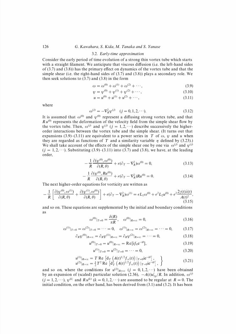
. (3.64)
In figure 7 we plot f(η)/(−D0eiϕ0 ) expressed by asymptotic solution (3.63) (dashedcurve) at Re = 1000 together with a numerical solution (solid curve) of (3.26) solvedby a shooting method, where thick and thin curves denote the real and imaginary
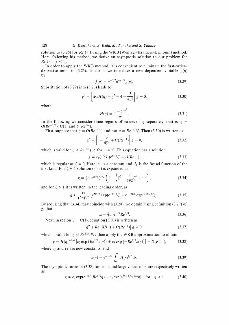
parts, respectively. The agreement between the two solutions is excellent except forrelatively small values of η. The region of disagreement should shrink as Re increases.In order to see the Reynolds number dependence we plot f(η) for two differentReynolds numbers on two different scales in figure 8. It oscillates more and morefrequently with increasing Reynolds number. The solution itself scales as Re1/2 atlarge η, while the envelope scales as Re1/3.
We next consider the vorticity component normal to the vortex tube. By using(2.47), (2.48) and (3.25), the normal components of the total vorticity ω = ×U +ω
can be expressed in terms of f(η) as
ω2 = A(t)−1/2Re f + 1
2ηf − 1
2ηf e−i2θ
, (3.65)
ω3 = A(t)−1/2Im
f + 1
2ηf + 1
2ηf e−i2θ
. (3.66)
8/3/2019 Genta Kawahara et al- Wrap, tilt and stretch of vorticity lines around a strong thin straight vortex tube in a simple …
http://slidepdf.com/reader/full/genta-kawahara-et-al-wrap-tilt-and-stretch-of-vorticity-lines-around-a-strong 19/49
132 G. Kawahara, S. Kida, M. Tanaka and S. Yanase
0 2η Re –1/3
–1.0
0
0.5
1.0
–0.5
f (η)
– D0 ei 0
1
(a)
0.5η Re –1/2
0
(b)
Figure 8. Reynolds number dependence of asymptotic solution (3.63). The real parts of solutionsare plotted against (a) ηRe−1/3 and (b) ηRe−1/2. Thick dashed and solid curves denote solutionsat Re = 1000 and 10000, respectively. Thin dashed and solid lines represent their envelopes,
± exp−(Re2/48η6)
.
If we use asymptotic forms (3.63) and (3.64), then (3.65) and (3.66) become
ω2 = − A(t)−1/2D0
cos
Re
4η2+ ϕ0
+
Re
2η2cos
Re
4η2+ ϕ0 − θ
sin θ
exp
− Re2
48η6
,
(3.67)
ω3 = − A(t)−1/2D0sin Re
4η2+ ϕ0
− Re2η2
cos Re4η2
+ ϕ0 − θ cos θ exp− Re2
48η6.
(3.68)
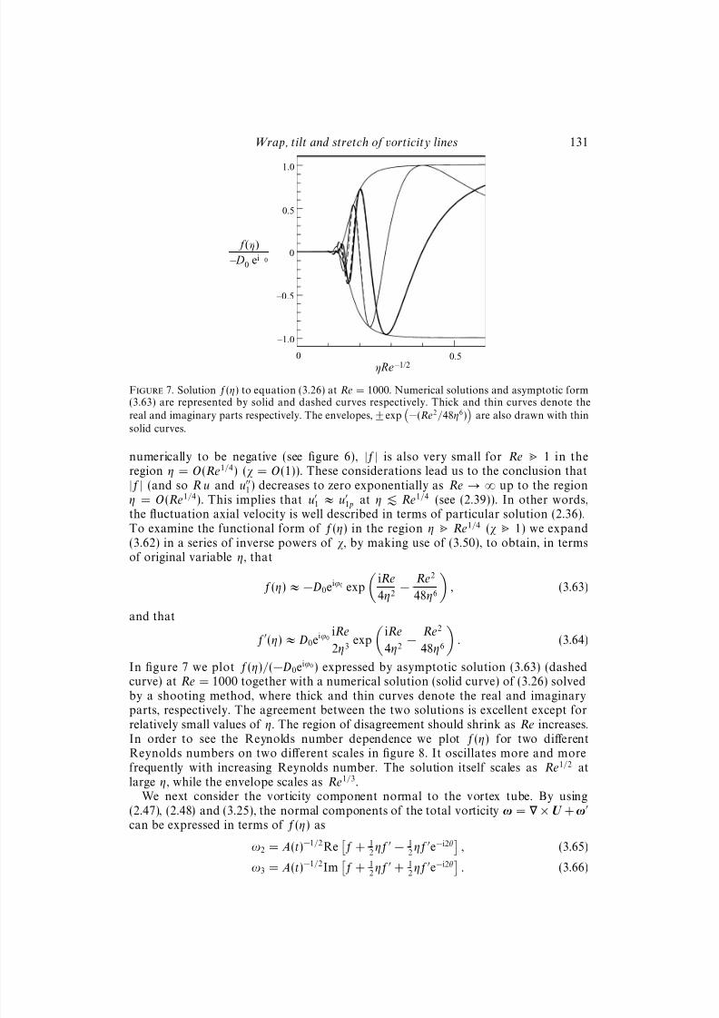
In figure 9 are shown the spatial distribution of normal vorticity (ω22 + ω2
3 )1/2 and theprojected vorticity lines on the normal (x2, x3)-plane, which were obtained from (3.67)and (3.68), at Re = 1000. Parts (a), (b) and (c) represent the cyclonic (α0 = arctan
√ 2,
β = − 14
π), neutral (α0 = 14
π, β = 0), and anticyclonic (α0 = arctan√
2, β = 14
π) cases,
in which the vortex tube is oriented in the direction of X 1 + X 2 − X 3, X 1 + X 2, and
X 1 +
X 2 +
X 3, respectively. Here, the relative magnitude of the normal vorticity is
represented by colour: the red is the highest (7S ) and the blue is the lowest (i.e.
zero). It can be seen that the vortex tube wraps and stretches vorticity lines aroundit to form two spiral vortex layers of high azimuthal vorticity oriented alternately
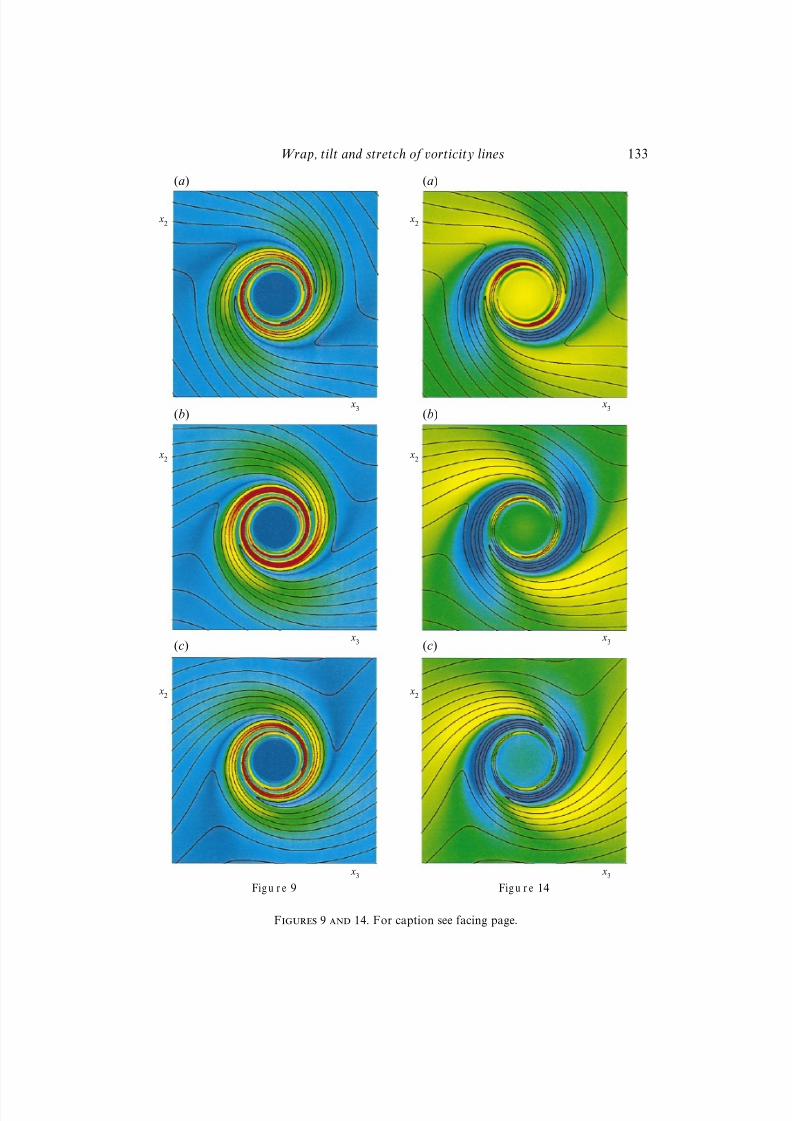
Figure 9. Spatial distribution of magnitude (ω22 + ω2
3 )1/2 of vorticity normal to a vortex tube at
Re = 1000 for (a) the cyclonic (α0 = arctan√
2, β = − 14
π), (b) neutral (α0 = 14
π, β = 0), and (c)
anticyclonic (α0 = arctan√
2, β = 14
π) cases. The level of the magnitude is represented by colour:red is the highest (7S ) and blue is the lowest (i.e. null). Solid curves represent vorticity lines projectedon the (x2, x3)-plane. A side length of the domain is 40 in similarity variable η. Two characteristiclength scales Re1/3 and Re1/2 are 10 and 31.6, respectively.
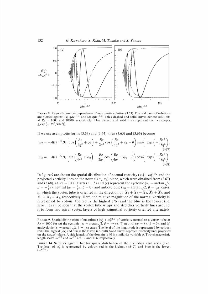
Figure 14. Same as figure 9 but for spatial distribution of the fluctuation axial vorticity ω1.
The level of ω1 is represented by colour: red is the highest (+S 2T ) and blue is the lowest
(−S 2T ).
8/3/2019 Genta Kawahara et al- Wrap, tilt and stretch of vorticity lines around a strong thin straight vortex tube in a simple …
http://slidepdf.com/reader/full/genta-kawahara-et-al-wrap-tilt-and-stretch-of-vorticity-lines-around-a-strong 20/49
Wrap, tilt and stretch of vorticity lines 133
(a)
(b)
(c)
(a)
(b)
(c)
x2
x2
x3
x3
x2
x2
x3
x3
x2
x2
x3
x3
Fig u r e 9 Fig u r e 14
Figures 9 and 14. For caption see facing page.
8/3/2019 Genta Kawahara et al- Wrap, tilt and stretch of vorticity lines around a strong thin straight vortex tube in a simple …
http://slidepdf.com/reader/full/genta-kawahara-et-al-wrap-tilt-and-stretch-of-vorticity-lines-around-a-strong 21/49
134 G. Kawahara, S. Kida, M. Tanaka and S. Yanase
in opposite directions. One of the most interesting features of the spirals is that the
x2-component of normal vorticity takes positive values in the outermost spiral layersof strong vorticity. It changes sign every time it makes a half-turn along the spirals.An important consequence of this change of sign will be discussed in §4.3.
In the near region (η . Re1/4, actually for η Re1/3), however, the excessivewrapping narrows the spacing of the spiral layers and enhances the viscous diffusionto cancel out their opposite-signed vorticities, which leads to the disappearance of thenormal vorticity around the vortex tube and to selective stretch-and-intensification of a cyclonic vortex tube (see §4.2).
The azimuthal vorticity component ωθ, which dominates the radial component (seethe vorticity lines in figure 9), is expressed as
ωθ = −ω2 sin θ + ω3 cos θ = − A(t)−1/2Re [i(ηf)e−iθ], (3.69)
which takes a local maximum and minimum,ωθmax
ωθmin
= ± A(t)−1/2|(ηf)| at
θmax
θmin
= arg[(ηf)] 1
2π. (3.70)
This implies that two spiral vortex layers of high azimuthal vorticity of opposite signof ωθ are arranged alternately. It follows from (3.63) and (3.64) that
(ηf) ≈ −D0eiϕ0
1 − iRe
2η2
exp
iRe
4η2− Re2
48η6
, (3.71)
the magnitude and phase of which are, respectively, written as
|(ηf)| ≈ D0
Re
2η2 1 +
4η4
Re21/2
exp
− Re2
48η6, (3.72)
arg[(ηf)] ≈ Re
4η2+ arctan
2η2
Re
+ ϕ0 + 1
2π. (3.73)
In figure 10 we plot (ηf)Re−1/3/(−D0eiϕ0 ) at Re = 1000, where solid and dashed curvesrepresent the real and imaginary parts respectively, and thin solid lines ±|(ηf)|. Wecan see that magnitude |(ηf)| has a single maximum of 0.903D0Re1/3 at η = 2−2/3Re1/3
(Moore 1985). It is exponentially small at η Re1/3, while it approaches a constantD0 = (cos2 α0 sin2 β + cos2 β)1/2, which is the magnitude of the normal component of the simple shear vorticity, as η increases. The phase, arg[(ηf)], is infinity at η = 0and decreases up to η = ( 1
2Re)1/2 at which it takes a minimum value of 1
2+ 3
4π + ϕ0,
and thereafter it increases monotonically to approach π + ϕ0 at η → ∞. Therefore,the spiral form of the layer actually terminates around η = ( 1
2
Re)1/2 since beyond this
point both θmax and θmin change only by 14
π − 12≈ 0.29 in the opposite direction.
The distance between adjacent layers of the two spirals is estimated as follows.Let η+ and η− be successive locations for a fixed value of θ of ωθmax and ωθmin,respectively, and let ∆η = η− − η+ be their spacing. Then, it follows from (3.70) and(3.73) that
Re
η2+
− Re
η2−= Re
(η+ + η−)
η2+η2−
∆η = 4π − 4 arctan
2η2
+
Re
+ 4 arctan
2η2−Re
, (3.74)
and therefore we have
∆η = O
η3
Re
(3.75)
8/3/2019 Genta Kawahara et al- Wrap, tilt and stretch of vorticity lines around a strong thin straight vortex tube in a simple …
http://slidepdf.com/reader/full/genta-kawahara-et-al-wrap-tilt-and-stretch-of-vorticity-lines-around-a-strong 22/49
Wrap, tilt and stretch of vorticity lines 135
0 1
η Re –1/3
–1.0
0
0.5
1.0
–0.5
2
(η f )′ Re –1/3
– D0 ei 0
Figure 10. Amplitude (ηf) of the circumferential component of vorticity ωθ. Solid and dashedcurves represent the real and imaginary parts respectively. Thin solid lines denote the magnitude,±|(ηf)|.
as long as η < ( 12
Re)1/2. The spacing between adjacent spiral layers is O(1) at
η = O(Re1/3).† It is greater than O(1) at O(Re1/3) < η
< ( 12
Re)1/2
. For Re1/3 η
( Re1/4), the spacing becomes very small as Re → ∞.In figure 9, in which a side length of the domain is 40 in similarity variable η, two
characteristic length scales Re1/3 and Re1/2 are 10 and 31.6, respectively. It is seen
that the double spiral vortex layer is developed at η = O(Re1/3
) and that it extendsup to η = O(Re1/2). Observe also that the spirals are terminated in the near region(η O(Re1/3)).
3.5. Higher-order axial vorticity
In this subsection we consider solutions to higher-order equation (3.15) for the axialvorticity. In order to get an explicit analytical solution, we restrict ourselves to early-time evolution (T 1). Since time T does not explicitly appear in the leading-orderstreamfunction (3.24), the first-order streamfunction and the corresponding axialvorticity may be expanded respectively as
ψ(1)(R ,θ ,T ) = T ψ(1,1)(η, θ) + T 2ψ(1,2)(η, θ) + · · · , (3.76)
ω(1)(R ,θ ,T ) = ω(1,0)(η, θ) + T ω(1,1)(η, θ) +
· · ·, (3.77)
where
ω(1,j −1) = − 142
ηψ(1,j ) (j = 1, 2, · · ·) (3.78)
with
2η = ∂2
η +1
η∂η +
1
η2∂2
θ . (3.79)
For small values of T , the time-dependent factors, γ/A, λ/A and ξ/A5/2 in linearoperators L1 and L2 (see (2.44) and (2.45)) are expanded in power series of T , using
† In dimensional variables, the location of the maximum normal vorticity isO
Re1/3(νT )1/2
and the spacing of the spirals is O
(νT )1/2
(see §4.4 and figure 19).
8/3/2019 Genta Kawahara et al- Wrap, tilt and stretch of vorticity lines around a strong thin straight vortex tube in a simple …
http://slidepdf.com/reader/full/genta-kawahara-et-al-wrap-tilt-and-stretch-of-vorticity-lines-around-a-strong 23/49
136 G. Kawahara, S. Kida, M. Tanaka and S. Yanase
α = α0
−T sin2 α0 cos β +
· · ·, as
γ
A=
cos α sin2 α sin β
sin α0
= γ0 + γ1T + · · · , (3.80)
λ
A= −sin2 α sin β
sin α0
= λ0 + λ1T + · · · , (3.81)
ξ
A5/2= −2sin9/2 α cos β
sin5/2 α0
= ξ0 + ξ1T + · · · , (3.82)
where
γ0 = γ|T =0 = cos α0 sin α0 cos β, γ1 = sin2 α0(1 − 3cos2 α0)cos2 β, (3.83)
λ0 = λ
|T =0 =
−sin α0 sin β, λ1 = 2 cos α0 sin2 α0 cos β sin β, (3.84)
ξ0 = ξ|T =0 = −2sin2 α0 cos β, ξ1 = −9cos α0 sin3 α0 cos2 β. (3.85)
Substituting (3.76), (3.77) and (3.80)–(3.82) into (3.15), and equating T −1-orderterms, we obtain
− 1
4η
∂(ψ(0), ω(1,0))
∂(η, θ)+
∂(ψ(1,1), ω(0,0))
∂(η, θ)
− 1
2η∂ηω(1,0) − 1
42
ηω(1,0) = L10ω(0,0), (3.86)
where
L10 = 12
[γ0(− sin2θ ∂θ + η cos2θ ∂η) + λ0(cos 2θ ∂θ + η sin2θ ∂η − ∂θ)] (3.87)
and
ω(0,0)(η) = T ω(0)(η) =1
4π
e−η2
. (3.88)
At T 0-order of (3.15), we have
− 1
4η
∂(ψ(0), ω(1,1))
∂(η, θ)+
∂(ψ(1,2), ω(0,0))
∂(η, θ)
+ (1 − 1
2η∂η)ω(1,1) − 1
42
ηω(1,1)
= L11ω(0,0) + 2L20u(0) + 22γ0λ0, (3.89)
where
L11 = 12
[γ1(− sin2θ ∂θ + η cos2θ ∂η) + λ1(cos 2θ ∂θ + η sin2θ ∂η − ∂θ)], (3.90)
L20 = ξ0[cos θ ∂θ + sin θ (η∂η + 1)]. (3.91)
The right-hand sides of (3.86) and (3.89) represent the effects of the simple shear onthe vorticity fluctuation. Asymptotic solutions to (3.86) and (3.89) at large Reynoldsnumbers (Re 1, 1) are derived in Appendices A and B. Here, we summarizethe results.
First, an asymptotic solution to (3.86) is written as
ω(1,0) = − 142
ηψ(1,1) = B0M 0(η) sin(2θ − φ0), (3.92)
where
M 0(η) = − η2
eη2 − 1
η2 − f1(η)
, (3.93)
and
B0 = (γ20 + λ2
0)1/2, φ0 = arctan
λ0
γ0
(3.94)
8/3/2019 Genta Kawahara et al- Wrap, tilt and stretch of vorticity lines around a strong thin straight vortex tube in a simple …
http://slidepdf.com/reader/full/genta-kawahara-et-al-wrap-tilt-and-stretch-of-vorticity-lines-around-a-strong 24/49
Wrap, tilt and stretch of vorticity lines 137
0 1η
1.0
0.5
– M 0
52 3 4
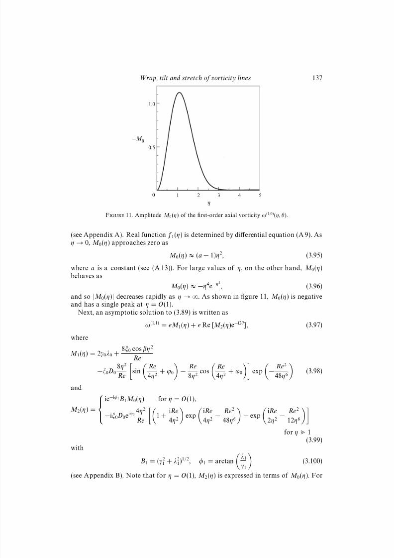
Figure 11. Amplitude M 0(η) of the first-order axial vorticity ω(1,0)(η, θ).
(see Appendix A). Real function f1(η) is determined by differential equation (A 9). Asη → 0, M 0(η) approaches zero as
M 0(η) ≈ (a − 1)η2, (3.95)
where a is a constant (see (A 13)). For large values of η, on the other hand, M 0(η)behaves as
M 0(η)
≈ −η4e−η2
, (3.96)
and so |M 0(η)| decreases rapidly as η → ∞. As shown in figure 11, M 0(η) is negativeand has a single peak at η = O(1).
Next, an asymptotic solution to (3.89) is written as
ω(1,1) = M 1(η) + Re [M 2(η)e−i2θ], (3.97)
where
M 1(η) = 2γ0λ0 +8ξ0 cos βη 2
Re
−ξ0D0
8η2
Re
sin
Re
4η2+ ϕ0
− Re
8η2cos
Re
4η2+ ϕ0
exp
− Re2
48η6
(3.98)
and
M 2(η) =
ie−iφ1 B1M 0(η) for η = O(1),
−iξ0D0eiϕ04η2
Re
1 +
iRe
4η2
exp
iRe
4η2− Re2
48η6
− exp
iRe
2η2− Re2
12η6
for η 1
(3.99)with
B1 = (γ21 + λ2
1)1/2, φ1 = arctan
λ1
γ1
(3.100)
(see Appendix B). Note that for η = O(1), M 2(η) is expressed in terms of M 0(η). For
8/3/2019 Genta Kawahara et al- Wrap, tilt and stretch of vorticity lines around a strong thin straight vortex tube in a simple …
http://slidepdf.com/reader/full/genta-kawahara-et-al-wrap-tilt-and-stretch-of-vorticity-lines-around-a-strong 25/49
138 G. Kawahara, S. Kida, M. Tanaka and S. Yanase
0η Re –1/2
0.5
–1.5
M 1
0.5
–1.0
–0.5
0
1.0
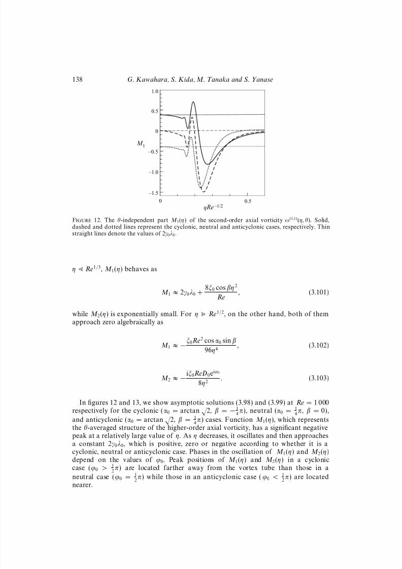
Figure 12. The θ-independent part M 1(η) of the second-order axial vorticity ω(1,1)(η, θ). Solid,dashed and dotted lines represent the cyclonic, neutral and anticyclonic cases, respectively. Thinstraight lines denote the values of 2γ0λ0.
η Re1/3, M 1(η) behaves as
M 1
≈2γ0λ0 +
8ξ0 cos βη2
Re
, (3.101)
while M 2(η) is exponentially small. For η Re1/2, on the other hand, both of themapproach zero algebraically as
M 1 ≈ −ξ0Re2 cos α0 sin β
96η4, (3.102)
M 2 ≈ − iξ0ReD0eiϕ0
8η2. (3.103)
In figures 12 and 13, we show asymptotic solutions (3.98) and (3.99) at Re = 1 000respectively for the cyclonic (α0 = arctan
√ 2, β = − 1
4π), neutral (α0 = 1
4π, β = 0),
and anticyclonic (α0 = arctan√
2, β = 14
π) cases. Function M 1(η), which representsthe θ-averaged structure of the higher-order axial vorticity, has a significant negativepeak at a relatively large value of η. As η decreases, it oscillates and then approachesa constant 2γ0λ0, which is positive, zero or negative according to whether it is acyclonic, neutral or anticyclonic case. Phases in the oscillation of M 1(η) and M 2(η)depend on the values of ϕ0. Peak positions of M 1(η) and M 2(η) in a cycloniccase (ϕ0 > 1
2π) are located farther away from the vortex tube than those in a
neutral case (ϕ0 = 12
π) while those in an anticyclonic case (ϕ0 < 12
π) are locatednearer.
8/3/2019 Genta Kawahara et al- Wrap, tilt and stretch of vorticity lines around a strong thin straight vortex tube in a simple …
http://slidepdf.com/reader/full/genta-kawahara-et-al-wrap-tilt-and-stretch-of-vorticity-lines-around-a-strong 26/49
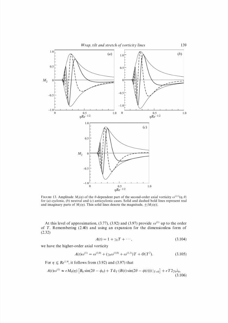
Wrap, tilt and stretch of vorticity lines 139
0η Re –1/2
0.5
M 2
0.5
–1.0
–0.5
0
1.0(a)
1.0 0η Re –1/2
0.5
(b)
1.0
0
η Re –1/2
0.5
M 2
0.5 –1.0
–0.5
0
1.0
(c)
1.0
0.5
–1.0
–0.5
0
1.0
Figure 13. Amplitude M 2(η) of the θ-dependent part of the second-order axial vorticity ω(1,1)(η, θ)for (a) cyclonic, (b) neutral and (c) anticyclonic cases. Solid and dashed bold lines represent realand imaginary parts of M 2(η). Thin solid lines denote the magnitude, ±|M 2(η)|.
At this level of approximation, (3.77), (3.92) and (3.97) provide ω(1) up to the order
of T . Remembering (2.40) and using an expansion for the dimensionless form of (2.32)
A(t) = 1 + γ0T + · · · , (3.104)
we have the higher-order axial vorticity
A(t)ω(1) = ω(1,0) + (γ0ω(1,0) + ω(1,1))T + O(T 2). (3.105)
For η . Re1/4, it follows from (3.92) and (3.97) that
A(t)ω(1) ≈ M 0(η)
B0 sin(2θ − φ0) + T dT (B(t) sin(2θ − φ(t))) |T =0
+ T 2γ0λ0,
(3.106)
8/3/2019 Genta Kawahara et al- Wrap, tilt and stretch of vorticity lines around a strong thin straight vortex tube in a simple …
http://slidepdf.com/reader/full/genta-kawahara-et-al-wrap-tilt-and-stretch-of-vorticity-lines-around-a-strong 27/49
140 G. Kawahara, S. Kida, M. Tanaka and S. Yanase
where we have used relation
B1 sin(2θ − φ1) = dT [B(t) sin(2θ − φ(t))] |T =0 − γ0B0 sin(2θ − φ0) (3.107)
with
B(t) =
γ(t)2 + λ(t)21/2
= | sin α|(cos2 α cos2 β + sin2 β)1/2 (3.108)
and
φ(t) = arctan
λ(t)
γ(t)
= arctan
− sin β
cos α cos β
(−π 6 φ(t) 6 π), (3.109)
which represents an angle from the x2-axis to a projection of the X 2-axis on thenormal (x2, x3)-plane (see (2.2) and (2.3)). Solution (3.106) represents the leading and
first orders of a Taylor expansion of A(t)ω(1) = M 0(η)B(t) sin(2θ − φ(t)) + ( A(t)λ0 − λ(t)). (3.110)
In the near region η . Re1/4, we can drop the second term on the right-hand side of (3.15), which is exponentially small as Re → ∞ (see §3.4). This tells us the importantfact that (3.110) may be obtained only by expanding ω(1) in a power series of without the short-time assumption T 1.
The first term on the right-hand side of (3.110) represents a quadrupole-typedistribution, which means a deformation of the vortex core into an elliptical shape bythe effect of the simple shear (Moffatt et al. 1994). The major and minor axes of theresulting elliptical core are aligned at an angle of θ = 1
2φ(t) + 1
2π ± 1
4π, respectively.
If the normal velocity components, (u2, u3), of the simple shear flow relative to
the structural coordinate system are decomposed into symmetric and antisymmetrictensors, we find that the symmetric one, which represents straining flow, has a principaldirection with a positive rate of strain at an angle of θ = 1
2φ(t) + 1
2π (the values of
rates of strain which are normalized by the uniform shear rate S are 12
(−γ(t) ± B(t))).Therefore, the major and minor axes of the ellipse are inclined away from the directionof strain by ± 1
4π, respectively (Moffatt et al. 1994). This quadrupole distribution of
vorticity, which does not include the stretch factor A(t), is not affected by the axialcomponent of the simple shear stress. In the case of α = 0, which was considered byPearson & Abernathy (1984) and Moore (1985), the vortex tube is aligned with thesimple shear flow and therefore the vortex core is not deformed ( B(t) ≡ 0).
The second term on the right-hand side of (3.110) represents the stretching of theaxial vorticity component of the simple shear by the axial stress (see §4.2).
4. Physical interpretation
A physical interpretation of the asymptotic solutions derived in §3 will be givenin this section to help understand the structure of vorticity field and the physicalprocess. We restore here dimensional variables, following table 1, as
T = T ∗/S , R = (ν/S )1/2R∗, ω1 = −1Sω∗
1 u1 = (νS )1/2u∗
1 . (4.1)
A similarity variable η is then η = (R∗/2T ∗1/2) = R/2(νT )1/2. Recall that the asterisks,which are attached to dimensionless variables, have been dropped in §3.
8/3/2019 Genta Kawahara et al- Wrap, tilt and stretch of vorticity lines around a strong thin straight vortex tube in a simple …
http://slidepdf.com/reader/full/genta-kawahara-et-al-wrap-tilt-and-stretch-of-vorticity-lines-around-a-strong 28/49
Wrap, tilt and stretch of vorticity lines 141
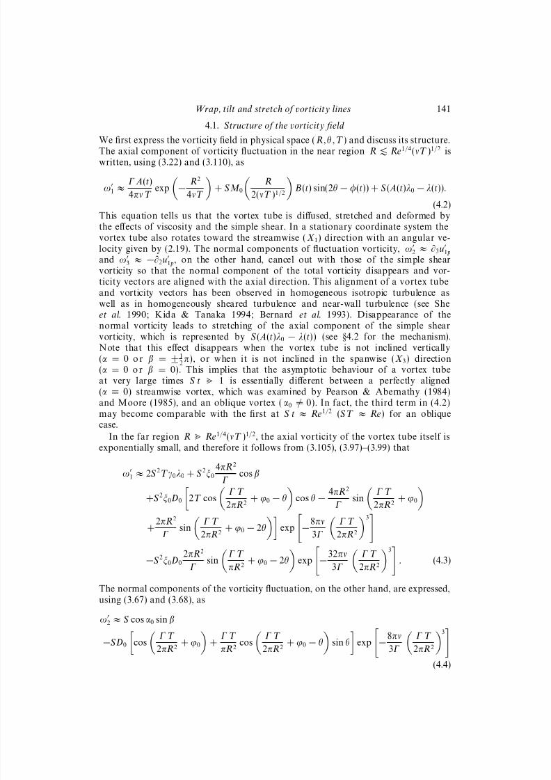
4.1. Structure of the vorticity field
We first express the vorticity field in physical space (R ,θ ,T ) and discuss its structure.The axial component of vorticity fluctuation in the near region R . Re1/4(νT )1/2 iswritten, using (3.22) and (3.110), as
ω1 ≈ Γ A(t)
4πν T exp
− R2
4νT
+ SM 0
R
2(νT )1/2
B(t) sin(2θ − φ(t)) + S ( A(t)λ0 − λ(t)).
(4.2)This equation tells us that the vortex tube is diffused, stretched and deformed bythe effects of viscosity and the simple shear. In a stationary coordinate system thevortex tube also rotates toward the streamwise (X 1) direction with an angular ve-locity given by (2.19). The normal components of fluctuation vorticity, ω
2 ≈ ∂3u1p
and ω3
≈ −∂2u
1p, on the other hand, cancel out with those of the simple shear
vorticity so that the normal component of the total vorticity disappears and vor-ticity vectors are aligned with the axial direction. This alignment of a vortex tubeand vorticity vectors has been observed in homogeneous isotropic turbulence aswell as in homogeneously sheared turbulence and near-wall turbulence (see Sheet al. 1990; Kida & Tanaka 1994; Bernard et al. 1993). Disappearance of thenormal vorticity leads to stretching of the axial component of the simple shearvorticity, which is represented by S ( A(t)λ0 − λ(t)) (see §4.2 for the mechanism).Note that this effect disappears when the vortex tube is not inclined vertically(α = 0 o r β = ± 1
2π), or when it is not inclined in the spanwise (X 3) direction
(α = 0 o r β = 0). This implies that the asymptotic behaviour of a vortex tubeat very large times S t 1 is essentially different between a perfectly aligned(α ≡ 0) streamwise vortex, which was examined by Pearson & Abernathy (1984)and Moore (1985), and an oblique vortex (α0
= 0). In fact, the third term in (4.2)
may become comparable with the first at S t ≈ Re1/2 (ST ≈ Re) for an obliquecase.
In the far region R Re1/4(νT )1/2, the axial vorticity of the vortex tube itself isexponentially small, and therefore it follows from (3.105), (3.97)–(3.99) that
ω1 ≈ 2S 2T γ0λ0 + S 2ξ0
4πR 2
Γcos β
+S 2ξ0D0
2T cos
Γ T
2πR2+ ϕ0 − θ
cos θ − 4πR2
Γsin
Γ T
2πR2+ ϕ0
+
2πR2
Γsin
Γ T
2πR2+ ϕ0 − 2θ
exp
−8πν
3Γ
Γ T
2πR2
3
−S 2ξ0D0
2πR2
ΓsinΓ T
πR2+ ϕ0 − 2θ
exp
−32πν
3Γ
Γ T
2πR2
3. (4.3)
The normal components of the vorticity fluctuation, on the other hand, are expressed,using (3.67) and (3.68), as
ω2 ≈ S cos α0 sin β
−SD0
cos
Γ T
2πR2+ ϕ0
+
Γ T
πR2cos
Γ T
2πR2+ ϕ0 − θ
sin θ
exp
−8πν
3Γ
Γ T
2πR2
3
(4.4)
8/3/2019 Genta Kawahara et al- Wrap, tilt and stretch of vorticity lines around a strong thin straight vortex tube in a simple …
http://slidepdf.com/reader/full/genta-kawahara-et-al-wrap-tilt-and-stretch-of-vorticity-lines-around-a-strong 29/49
142 G. Kawahara, S. Kida, M. Tanaka and S. Yanase
and
ω3 ≈ S cos β − S D0
sin Γ T
2πR2+ ϕ0
−Γ T
πR2cos
Γ T
2πR2+ ϕ0 − θ
cos θ
exp
−8πν
3Γ
Γ T
2πR2
3
. (4.5)
The spatial distributions on the normal plane of axial vorticity fluctuation (4.3) aredrawn in figure 14 (see p. 133) for (a) cyclonic (α0 = arctan
√ 2, β = − 1
4π), (b) neutral
(α0 = 14
π, β = 0) and (c) anticyclonic (α0 = arctan√
2, β = 14
π) cases at Re = 1000together with projected vorticity lines. The vorticity of the vortex tube itself is notshown in these figures. Along vorticity lines at the outermost double spirals of highazimuthal vorticity there are two crescent-shaped regions of strong negative axial
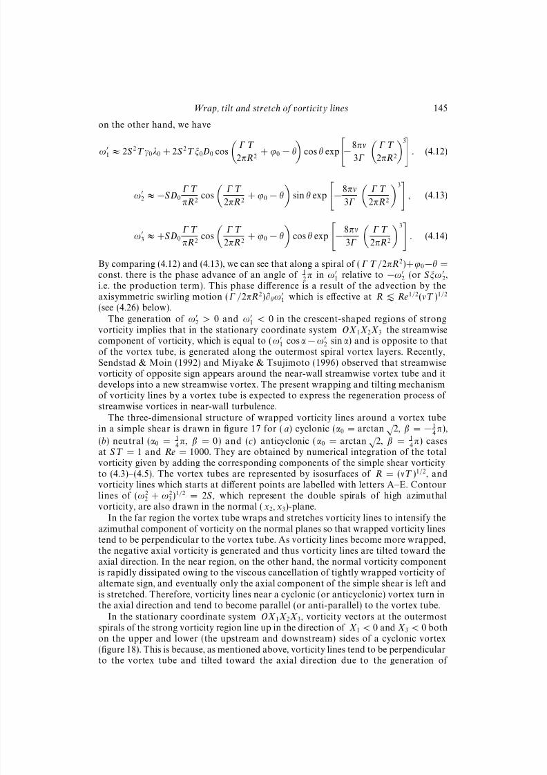
vorticity, which is opposite to the vorticity of the vortex tube (cf. figure 9). Alsocommonly observed is relatively weak positive vorticity inside the crescent-shapedregions of negative vorticity. Further inside, i.e. in a circular domain in the vicinity of a cyclonic (or anticyclonic) vortex tube the axial vorticity takes positive (or negative)values. The appearance of negative vorticity in the far region as well as different signsof vorticity in the central region between cyclonic and anticyclonic vortex tubes werealso observed in the θ-averaged structure (see figure 12).
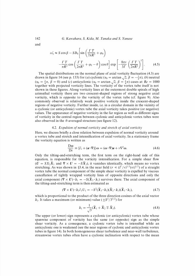
4.2. Expulsion of normal vorticity and stretch of axial vorticity
Here, we discuss briefly a close relation between expulsion of normal vorticity arounda vortex tube and stretch and intensification of axial vorticity. In a stationary framethe vorticity equation is written as
Dω
Dt≡ [∂t + (u · )]ω = (ω · )u + ν2
ω. (4.6)
Only the tilting-and-stretching term, the first term on the right-hand side of thisequation, is responsible for the vorticity intensification. For a simple shear flow
(U = S X 2 X 1 and × U = −S X 3), it vanishes identically, which means no vortexstretching. As was shown in §3.4, in the near field (r (Γ /ν)1/3(νt)1/2) of a straightvortex tube the normal component of the simple shear vorticity is expelled by viscouscancellation of tightly wrapped vorticity lines of opposite directions and only the
axial component ( × U ) · x1 = −S ( X 3 · x1) survives there. The axial component of the tilting-and-stretching term is then estimated as
(
×U ) · x1∂1U1 =
−S 2( X 3 · x1)( X 2 · x1)( X 1 · x1), (4.7)
which is proportional to the product of the three direction cosines of the axial vector x1. It takes a maximum (or minimum) value (±S 2/33/2) for
x1 =1√
3( X 1 + X 2 X 3). (4.8)
The upper (or lower) sign represents a cyclonic (or anticyclonic) vortex tube whosespanwise component of vorticity has the same (or opposite) sign as the simpleshear vorticity. As a consequence, a cyclonic vortex tube is intensified while ananticyclonic one is weakened (see the near regions of cyclonic and anticyclonic vortextubes in figure 14). In both homogeneous shear turbulence and near-wall turbulence,streamwise vortex tubes often have a cyclonic inclination with respect to the mean
8/3/2019 Genta Kawahara et al- Wrap, tilt and stretch of vorticity lines around a strong thin straight vortex tube in a simple …
http://slidepdf.com/reader/full/genta-kawahara-et-al-wrap-tilt-and-stretch-of-vorticity-lines-around-a-strong 30/49
Wrap, tilt and stretch of vorticity lines 143
x 2
x 3
] × U
Figure 15. Generation mechanism of axial vorticity along spiral layers of high azimuthal vorticitywhich are represented by crescent-shaped shadow regions. Double arrows denote the direction of normal vorticity. and ⊗ denote the direction of axial velocity induced by the spiral vorticity layersby which the simple shear vorticity × U is tilted toward the axial direction.
shear vorticity (see Kida & Tanaka 1994; Miyake & Tsujimoto 1996), which may beconnected with the above mechanism of selective intensification of a cyclonic vortex.
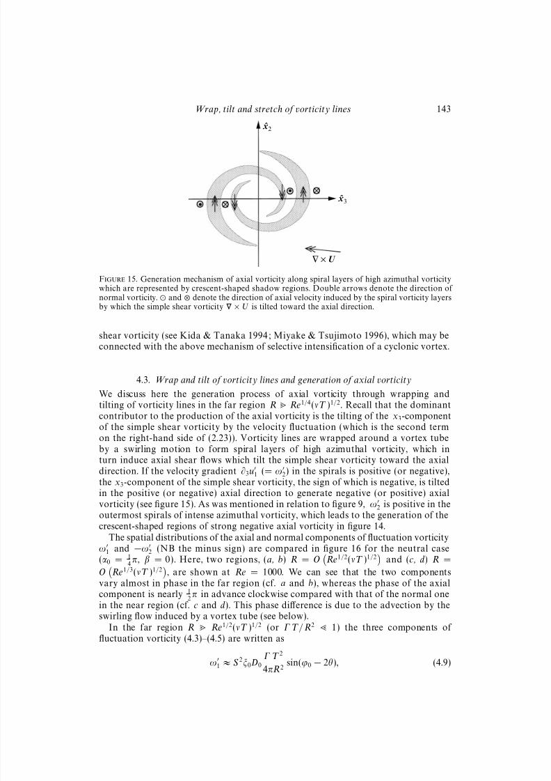
4.3. Wrap and tilt of vorticity lines and generation of axial vorticity
We discuss here the generation process of axial vorticity through wrapping andtilting of vorticity lines in the far region R Re1/4(νT )1/2. Recall that the dominantcontributor to the production of the axial vorticity is the tilting of the x3-componentof the simple shear vorticity by the velocity fluctuation (which is the second termon the right-hand side of (2.23)). Vorticity lines are wrapped around a vortex tubeby a swirling motion to form spiral layers of high azimuthal vorticity, which inturn induce axial shear flows which tilt the simple shear vorticity toward the axialdirection. If the velocity gradient ∂3u
1 (= ω2) in the spirals is positive (or negative),
the x3-component of the simple shear vorticity, the sign of which is negative, is tiltedin the positive (or negative) axial direction to generate negative (or positive) axialvorticity (see figure 15). As was mentioned in relation to figure 9, ω
2 is positive in theoutermost spirals of intense azimuthal vorticity, which leads to the generation of thecrescent-shaped regions of strong negative axial vorticity in figure 14.
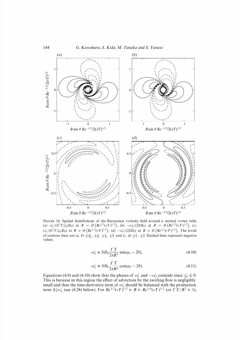
The spatial distributions of the axial and normal components of fluctuation vorticity
ω1 and −ω2 (NB the minus sign) are compared in figure 16 for the neutral case(α0 = 1
4π, β = 0). Here, two regions, (a, b) R = O
Re1/2(νT )1/2
and (c, d) R =
O
Re1/3(νT )1/2
, are shown at Re = 1000. We can see that the two componentsvary almost in phase in the far region (cf. a and b), whereas the phase of the axialcomponent is nearly 1
2π in advance clockwise compared with that of the normal one
in the near region (cf. c and d). This phase difference is due to the advection by theswirling flow induced by a vortex tube (see below).
In the far region R Re1/2(νT )1/2 (or ΓT/R2 1) the three components of
fluctuation vorticity (4.3)–(4.5) are written as
ω1 ≈ S 2ξ0D0
Γ T 2
4πR2sin(ϕ0 − 2θ), (4.9)
8/3/2019 Genta Kawahara et al- Wrap, tilt and stretch of vorticity lines around a strong thin straight vortex tube in a simple …
http://slidepdf.com/reader/full/genta-kawahara-et-al-wrap-tilt-and-stretch-of-vorticity-lines-around-a-strong 31/49
144 G. Kawahara, S. Kida, M. Tanaka and S. Yanase
(a)
1
0
–1
–1 0 1
R c o s θ R e – 1 / 2 / 2 ( m T ) 1 / 2
Rsin θ Re –1/2/2(mT )1/2
(b)
1
0
–1
–1 0 1
Rsin θ Re –1/2/2(mT )1/2
(c)
0.5
0
–0.5
–0.5 0 0.5
R c o s θ R e – 1 / 3 / 2 ( m T ) 1 / 2
Rsin θ Re –1/3/2(mT )1/2
(d )
0.5
0
–0.5
–0.5 0 0.5
Rsin θ Re –1/3/2(mT )1/2
Figure 16. Spatial distributions of the fluctuation vorticity field around a neutral vortex tube.
(a) ω1/(S 2T |ξ0|D0) at R = O
Re1/2(νT )1/2
, (b) −ω
2/(2SD0) at R = O
Re1/2(νT )1/2
, (c)
ω1/(S 2T |ξ0|D0) at R = O
Re1/3(νT )1/2
, (d) −ω
2/(2SD0) at R = O
Re1/3(νT )1/2
. The levels
of contour lines are (a, b)
±1
16
,
±1
8
,
±1
4
,
±1
2
and (c, d)
±1
2
,
±2. Dashed lines represent negative
values.
ω2 ≈ S D0
Γ T
2πR2sin(ϕ0 − 2θ), (4.10)
ω3 ≈ S D0
Γ T
2πR2cos(ϕ0 − 2θ). (4.11)
Equations (4.9) and (4.10) show that the phases of ω1 and −ω
2 coincide since ξ0 6 0.This is because in this region the effect of advection by the swirling flow is negligiblysmall and thus the time-derivative term of ω
1 should be balanced with the productionterm Sξω
2 (see (4.26) below). For Re1/2(νT )1/2 R Re1/4(νT )1/2 (or ΓT/R2
1),
8/3/2019 Genta Kawahara et al- Wrap, tilt and stretch of vorticity lines around a strong thin straight vortex tube in a simple …
http://slidepdf.com/reader/full/genta-kawahara-et-al-wrap-tilt-and-stretch-of-vorticity-lines-around-a-strong 32/49
Wrap, tilt and stretch of vorticity lines 145
on the other hand, we have
ω1 ≈ 2S 2T γ0λ0 + 2S 2T ξ0D0 cos
Γ T
2πR2+ ϕ0 − θ
cos θ exp
−8πν
3Γ
Γ T
2πR2
3. (4.12)
ω2 ≈ −SD0
Γ T
πR2cos
Γ T
2πR 2+ ϕ0 − θ
sin θ exp
−8πν
3Γ
Γ T
2πR2
3
, (4.13)
ω3 ≈ +SD0
Γ T
πR2cos
Γ T
2πR 2+ ϕ0 − θ
cos θ exp
−8πν
3Γ
Γ T
2πR2
3
. (4.14)
By comparing (4.12) and (4.13), we can see that along a spiral of (Γ T /2πR2)+ϕ0
−θ =
const. there is the phase advance of an angle of 12 π in ω
1 relative to −ω2 (or Sξω
2,i.e. the production term). This phase difference is a result of the advection by theaxisymmetric swirling motion (Γ /2πR2)∂θω
1 which is effective at R . Re1/2(νT )1/2
(see (4.26) below).The generation of ω
2 > 0 and ω1 < 0 in the crescent-shaped regions of strong
vorticity implies that in the stationary coordinate system OX 1X 2X 3 the streamwisecomponent of vorticity, which is equal to (ω
1 cos α − ω2 sin α) and is opposite to that
of the vortex tube, is generated along the outermost spiral vortex layers. Recently,Sendstad & Moin (1992) and Miyake & Tsujimoto (1996) observed that streamwisevorticity of opposite sign appears around the near-wall streamwise vortex tube and itdevelops into a new streamwise vortex. The present wrapping and tilting mechanismof vorticity lines by a vortex tube is expected to express the regeneration process of
streamwise vortices in near-wall turbulence.The three-dimensional structure of wrapped vorticity lines around a vortex tube
in a simple shear is drawn in figure 17 for (a) cyclonic (α0 = arctan√
2, β = − 14
π),
(b) neutral (α0 = 14
π, β = 0) and (c) anticyclonic (α0 = arctan√
2, β = 14
π) casesat ST = 1 and Re = 1000. They are obtained by numerical integration of the totalvorticity given by adding the corresponding components of the simple shear vorticityto (4.3)–(4.5). The vortex tubes are represented by isosurfaces of R = (νT )1/2, andvorticity lines which starts at different points are labelled with letters A–E. Contourlines of (ω2
2 + ω23 )1/2 = 2S , which represent the double spirals of high azimuthal
vorticity, are also drawn in the normal (x2, x3)-plane.In the far region the vortex tube wraps and stretches vorticity lines to intensify the
azimuthal component of vorticity on the normal planes so that wrapped vorticity lines
tend to be perpendicular to the vortex tube. As vorticity lines become more wrapped,the negative axial vorticity is generated and thus vorticity lines are tilted toward theaxial direction. In the near region, on the other hand, the normal vorticity componentis rapidly dissipated owing to the viscous cancellation of tightly wrapped vorticity of alternate sign, and eventually only the axial component of the simple shear is left andis stretched. Therefore, vorticity lines near a cyclonic (or anticyclonic) vortex turn inthe axial direction and tend to become parallel (or anti-parallel) to the vortex tube.
In the stationary coordinate system OX 1X 2X 3, vorticity vectors at the outermostspirals of the strong vorticity region line up in the direction of X 1 < 0 and X 3 < 0 bothon the upper and lower (the upstream and downstream) sides of a cyclonic vortex(figure 18). This is because, as mentioned above, vorticity lines tend to be perpendicularto the vortex tube and tilted toward the axial direction due to the generation of
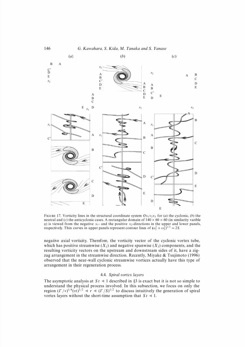
8/3/2019 Genta Kawahara et al- Wrap, tilt and stretch of vorticity lines around a strong thin straight vortex tube in a simple …
http://slidepdf.com/reader/full/genta-kawahara-et-al-wrap-tilt-and-stretch-of-vorticity-lines-around-a-strong 33/49
146 G. Kawahara, S. Kida, M. Tanaka and S. Yanase
(a)
AB
C′D
E
x2
ABC
DE x3
x1
C′
A
B
C
D
E
(b)
BC′
DE
x2
ABCD
x3
x1
C′
A
B
C
D
(c)
C′
DE
x2A B
C
D
x3
x1
A
B
C
D
E
E
A
E
E
BA
E
B
A
C′
D
Figure 17. Vorticity lines in the structural coordinate system Ox1x2x3 for (a) the cyclonic, (b) theneutral and (c) the anticyclonic cases. A rectangular domain of 140 × 60 × 60 (in similarity varibleη) is viewed from the negative x1- and the positive x2-directions in the upper and lower panels,respectively. Thin curves in upper panels represent contour lines of (ω2
2 + ω23 )1/2 = 2S .
negative axial vorticity. Therefore, the vorticity vector of the cyclonic vortex tube,which has positive streamwise (X 1) and negative spanwise (X 3) components, and theresulting vorticity vectors on the upstream and downstream sides of it, have a zig-zag arrangement in the streamwise direction. Recently, Miyake & Tsujimoto (1996)observed that the near-wall cyclonic streamwise vortices actually have this type of arrangement in their regeneration process.
4.4. Spiral vortex layers
The asymptotic analysis at S t 1 described in §3 is exact but it is not so simple tounderstand the physical process involved. In this subsection, we focus on only theregion (Γ /ν)1/4(νt)1/2
r (Γ /S )1/2 to discuss intuitively the generation of spiralvortex layers without the short-time assumption that S t 1.
8/3/2019 Genta Kawahara et al- Wrap, tilt and stretch of vorticity lines around a strong thin straight vortex tube in a simple …
http://slidepdf.com/reader/full/genta-kawahara-et-al-wrap-tilt-and-stretch-of-vorticity-lines-around-a-strong 34/49
Wrap, tilt and stretch of vorticity lines 147
X 1
A A E E
X 3
Figure 18. Vorticity lines distorted by a cyclonic vortex tube in the stationary coordinate systemOX 1X 2X 3. Lines A and E are the same as the corresponding ones in figure 17. Note that thestreamwise (X 1) component of vorticity of distorted vorticity lines (which is negative) is opposite tothat of the vortex tube (which is positive).
The flow structure in the far region r (Γ /ν)1/4(νt)1/2 may be analysed moresimply by replacing the vortex tube with a filament. Separating the contribution fromthe vortex filament in the streamfunction as
ψ = −Γ
2π ln r + ψ, (4.15)
and substituting it into (2.23) and (2.24), we obtain
∂tω1 − ∂(ψ, ω
1)
∂(x2, x3)+
Γ
2πr2∂θω
1 − S (γ(t)x2 + λ(t)x3)∂2ω1
= S γ(t)ω1 + Sξ(t)∂3u
1 + ν2⊥ω
1 (4.16)
and
∂tu1 − ∂(ψ, u
1)
∂(x2, x3)+
Γ
2πr2∂θu
1 − S (γ(t)x2 + λ(t)x3)∂2u1
= −S γ(t)u1 +
Γ S
2πr2 (cos α sin β x2 + cos β x3) − S (cos α sin β ∂2 + cos β ∂3)ψ + ν2
⊥u1.(4.17)
These equations are supplemented by initial conditions, ω1 = 0 and u
1 = 0.
We first consider the behaviour of the velocity field deformed by a strong vortexfilament, and suppose that
Γ
ν 1. (4.18)
Within r (Γ /S )1/2, the velocity induced by the filament dominates the simple shearvelocity. It is the first and third terms on the left-hand side and the second term onthe right-hand side that are dominant in (4.17) except for the viscous term which will
8/3/2019 Genta Kawahara et al- Wrap, tilt and stretch of vorticity lines around a strong thin straight vortex tube in a simple …
http://slidepdf.com/reader/full/genta-kawahara-et-al-wrap-tilt-and-stretch-of-vorticity-lines-around-a-strong 35/49
148 G. Kawahara, S. Kida, M. Tanaka and S. Yanase
be taken into account below. Then we have
∂tu1 +
Γ2πr2
∂θu1 =
Γ S 2πr2
(cos α sin β x2 + cos β x3). (4.19)
This has a solution
u1 = SD0r sin
Γ t
2πr2+ ϕ0 − θ
− SD(t)r sin(ϕ(t) − θ), (4.20)
which represents spiral vortex layers, where D0 and ϕ0, and D(t) and ϕ(t) are givenby (3.4) and (2.38), respectively.
In order to take account of the effect of viscous diffusion, we introduce unknownfunctions s1(r, t) and s2(r, t) as
u1
= s1(r, t)cosθ−
Γ t
2πr2+ s2(r, t)sinθ−
Γ t
2πr2−SD(t)r sin(ϕ(t)
−θ). (4.21)
In the region r (Γ /ν)1/4(νt)1/2 (which can exist if S t (Γ /ν)1/2) the viscous termmay be approximated by
ν2⊥u
1 ≈ −4ν
Γ t
2πr3
2 s1 cos
θ − Γ t
2πr2
+ s2 sin
θ − Γ t
2πr2
. (4.22)
Substitution of (4.21) and (4.22) into (4.19) plus the viscous term gives a set of differential equations for s1 and s2, which are solved easily under initial conditionu
1 = 0, i.e. s1|t=0 = S r cos β, s2|t=0 = −Sr cos α0 sin β to yield
u1 = SD0r sin
Γ t
2πr2
+ ϕ0
−θ exp−
8πν
3Γ Γ t
2πr2
3
−SD(t)r sin(ϕ(t)
−θ). (4.23)
This is a viscous version of (4.20).The x2- and x3-components of the fluctuation vorticity are then calculated to be
ω2 = ∂3u
1 = S cos α sin β
−SD0
cos
Γ t
2πr2+ ϕ0
+
Γ t
πr2cos
Γ t
2πr2+ ϕ0 − θ
sin θ
exp
−8πν
3Γ
Γ t
2πr2
3
(4.24)
and
ω3 =
−∂2u
1 = S cos β
−SD0
sin Γ t
2πr2+ ϕ0
− Γ t
πr2cos
Γ t2πr2
+ ϕ0 − θ
cos θ
exp−8πν
3Γ Γ t
2πr2
3,
(4.25)
which agree with (4.4) and (4.5) for S t 1. The x2-component of the fluctuationvorticity (4.24) appears in axial-vorticity equation (4.16) as a source term.
In the near-field r (Γ /S )1/2 and during the period S t (Γ /ν)1/2 the dominantterms in (4.16) are the first and third terms on the left-hand side and the second andthird terms on the right-hand side. Then we have
∂tω1 +
Γ
2πr2∂θω
1 = Sξ(t)∂3u1 + ν2
⊥ω1. (4.26)
8/3/2019 Genta Kawahara et al- Wrap, tilt and stretch of vorticity lines around a strong thin straight vortex tube in a simple …
http://slidepdf.com/reader/full/genta-kawahara-et-al-wrap-tilt-and-stretch-of-vorticity-lines-around-a-strong 36/49
Wrap, tilt and stretch of vorticity lines 149
A solution to this equation under initial condition ω1
|t=0 = 0 is
ω1 = S ( A(t)λ0 − λ(t)) +
1 + O
ν
Γ
S 2ξ(t)
4πr2
Γcos β
+S 2ξ(t)D0
2t cos
Γ t
2πr2+ ϕ0 − θ
cos θ − 4πr2
Γsin
Γ t
2πr2+ ϕ0
+
2πr2
Γsin
Γ t
2πr2+ ϕ0 − 2θ
exp
−8πν
3Γ
Γ t
2πr2
3
−S 2ξ(t)D0
2πr2
Γsin
Γ t
πr2+ ϕ0 − 2θ
exp
−32πν
3Γ
Γ t
2πr2
3
, (4.27)
which agrees with (4.3) for S t 1. If we restrict ourselves in a period 1 . S t
(Γ /ν)1/2 (and so the region (Γ /ν)1/4(νt)1/2 r (Γ /ν)1/2(νt)1/2), four terms contain-ing O(S 2r2/Γ ) may be neglected in (4.27). Incidentally, a spiral vortex solution whichrepresents the wrapping of the axial component of vorticity by an axisymmetricswirling flow was obtained by Lundgren (1982). Our solution (4.27), on the otherhand, describes the conversion of normal vorticity to the axial direction by shearingmotion induced by wrapped spiral vortex layers of high azimuthal vorticity. Thus,these two are essentially different from each other.
It should be emphasized that solutions (4.24), (4.25) and (4.27) have been obtainedfor (Γ /ν)1/4(νt)1/2
r (Γ /S )1/2 without the short-time assumption that S t 1. Asimilarity in the functional forms between asymptotic solutions (4.3)–(4.5) and (4.24),(4.25) and (4.27) suggests that the former may be approximated well even for S t ≈ 1.
The position of the maximum normal vorticity and spacing of the spirals areintuitively estimated as follows. The spirals of high azimuthal vorticity are primarilygenerated by a strong swirling potential velocity induced by the vortex tube in theform (see the first term of (4.20))
θ − Γ t
2πr2= const. (4.28)
The spacing ∆r of the spiral is given by the change of r when angle θ changes by 2π,so that it follows from (4.28) that
Γ t
r3∆r ≈ 1. (4.29)
The region in which viscous effects play a role is estimated by equating the viscousand the time-derivative terms
1t
≈ ν Γ tr32
, (4.30)
or
r ≈
Γ
ν
1/3
(νt)1/2. (4.31)
Combination of (4.29) and (4.31) yields
∆r ≈ (νt)1/2. (4.32)
Finally, we discuss intuitively the order of magnitude of the axial vorticity generatedthrough the tilting of the x3-component of the simple shear vorticity by the spiralvortex layers. The gradient of axial velocity across the spirals may be estimated, by
8/3/2019 Genta Kawahara et al- Wrap, tilt and stretch of vorticity lines around a strong thin straight vortex tube in a simple …
http://slidepdf.com/reader/full/genta-kawahara-et-al-wrap-tilt-and-stretch-of-vorticity-lines-around-a-strong 37/49
150 G. Kawahara, S. Kida, M. Tanaka and S. Yanase
using (4.29), as
u1∆r
≈ S Γ tr2
, (4.33)
which works to tilt the simple shear vorticity toward the axial direction. In the region(Γ /ν)1/2(νt)1/2
r (Γ /ν)1/4(νt)1/2 the time scale of the time-derivative term is muchsmaller than that of the advection term because of the swirling flow,
1
t
Γ
r2, (4.34)
so that the former may dominate the latter and balance the production term in (4.26).Thus we have
Γ
r2ω
1 ≈ S 2Γ t
r2, (4.35)
that is, the axial vorticity increases in time asω
1 ≈ S 2t. (4.36)
In the region r ≈ (Γ /ν)1/2(νt)1/2 (which can exist if S t 1), on the other hand, thetwo time scales are comparable,
1
t≈ Γ
r2, (4.37)
and we have
ω1 ≈ S 2t ≈ S 2
Γ t2
r2≈ S 2
r2
Γ, (4.38)
which increases with radial distance. Therefore, the magnitude of ω1 can be strongest
near the outermost spirals at least during the initial time S t 1 of evolution because
there is no spiral and so ω1 decays at r & (Γ /ν)1/2(νt)1/2.
5. Concluding remarks
Asymptotic solutions describing the interactions between a straight vortex tube of circulation Γ starting with a vortex filament and a simple shear flow of shear rate S have been obtained at a large Reynolds number Γ /ν 1 and at an early time S t 1of evolution as well as S t (Γ /ν)1/2 for (Γ /ν)1/4(νt)1/2
r (Γ /S )1/2 (see §4.4).These solutions are expected to be useful for understanding interactions of tube-likestructures with background vorticity in real turbulent flows.
Let us now summarize the global structure of the present vorticity field in termsof the original physical coordinate r and time t. A thin strong straight vortex tube
which starts with a filament is diffused by viscosity and the core size increases intime as (νt)1/2 (see figure 19). This vortex tube induces an axisymmetric swirlingflow around it, which dominates the simple shear velocity in the near region wherer (Γ /S )1/2. The simple shear vorticity (denoted by double arrows) is stretched andwrapped by this swirling flow to make double spirals around the vortex tube. Thestretching (in planes normal to the vortex tube) of the vorticity lines is more effectiveand the intensity of the vorticity is enhanced more near the vortex tube becausethe swirling motion is more rapid there. Therefore the magnitude of the azimuthalcomponents of the vorticity increases as it approaches the vortex tube. The rapidswirling motion around the vortex tube also makes the spirals wind so tightly thatviscous effects may become important there. Because the azimuthal vorticity changesdirection alternately on neighouring layers of spirals, viscous diffusion smooths out
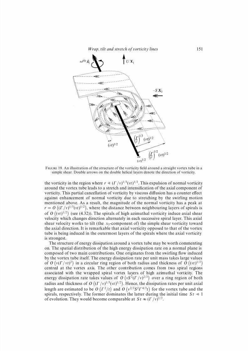
8/3/2019 Genta Kawahara et al- Wrap, tilt and stretch of vorticity lines around a strong thin straight vortex tube in a simple …
http://slidepdf.com/reader/full/genta-kawahara-et-al-wrap-tilt-and-stretch-of-vorticity-lines-around-a-strong 38/49
Wrap, tilt and stretch of vorticity lines 151
U X ˆ1
–S X ˆ3
ω(0) x 1
(νt )1/2
(νt )1/2
ν
1/3 (νt )1/2
ν
1/2 (νt )1/2
Figure 19. An illustration of the structure of the vorticity field around a straight vortex tube in asimple shear. Double arrows on the double helical layers denote the direction of vorticity.
the vorticity in the region where r
(Γ /ν)1/3
(νt)1/2
. This expulsion of normal vorticityaround the vortex tube leads to a stretch and intensification of the axial component of vorticity. This partial cancellation of vorticity by viscous diffusion has a counter effectagainst enhancement of normal vorticity due to stretching by the swirling motionmentioned above. As a result, the magnitude of the normal vorticity has a peak atr = O
(Γ /ν)1/3(νt)1/2
, where the distance between neighbouring layers of spirals is
of O
(νt)1/2
(see (4.32)). The spirals of high azimuthal vorticity induce axial shearvelocity which changes direction alternately in each successive spiral layer. This axialshear velocity works to tilt (the x3-component of) the simple shear vorticity towardthe axial direction. It is remarkable that axial vorticity opposed to that of the vortextube is being induced in the outermost layers of the spirals where the axial vorticityis strongest.
The structure of energy dissipation around a vortex tube may be worth commentingon. The spatial distribution of the high energy dissipation rate on a normal plane iscomposed of two main contributions. One originates from the swirling flow inducedby the vortex tube itself. The energy dissipation rate per unit mass takes large valuesof O
ν(Γ/νt)2
in a circular ring region of both radius and thickness of O
(νt)1/2
centred at the vortex axis. The other contribution comes from two spiral regionsassociated with the wrapped spiral vortex layers of high azimuthal vorticity. Theenergy dissipation rate takes values of O
νS 2(Γ /ν)2/3
over a ring region of both
radius and thickness of O
(Γ /ν)1/3(νt)1/2
. Hence, the dissipation rates per unit axial
length are estimated to be O
Γ 2/t
and O
ν2/3S 2Γ 4/3t
for the vortex tube and thespirals, respectively. The former dominates the latter during the initial time S t 1of evolution. They would become comparable at S t ≈ (Γ /ν)1/3.
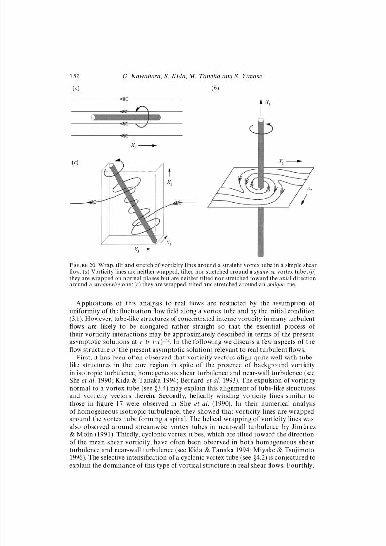
8/3/2019 Genta Kawahara et al- Wrap, tilt and stretch of vorticity lines around a strong thin straight vortex tube in a simple …
http://slidepdf.com/reader/full/genta-kawahara-et-al-wrap-tilt-and-stretch-of-vorticity-lines-around-a-strong 39/49
152 G. Kawahara, S. Kida, M. Tanaka and S. Yanase
(a)
X 3
(c)
X 3
X 2
X 1
(b)
X 3
X 2
X 1
Figure 20. Wrap, tilt and stretch of vorticity lines around a straight vortex tube in a simple shearflow. (a) Vorticity lines are neither wrapped, tilted nor stretched around a spanwise vortex tube; (b)they are wrapped on normal planes but are neither tilted nor stretched toward the axial direction
around a streamwise one; (c) they are wrapped, tilted and stretched around an oblique one.
Applications of this analysis to real flows are restricted by the assumption of uniformity of the fluctuation flow field along a vortex tube and by the initial condition(3.1). However, tube-like structures of concentrated intense vorticity in many turbulentflows are likely to be elongated rather straight so that the essential process of their vorticity interactions may be approximately described in terms of the presentasymptotic solutions at r (νt)1/2. In the following we discuss a few aspects of theflow structure of the present asymptotic solutions relevant to real turbulent flows.
First, it has been often observed that vorticity vectors align quite well with tube-like structures in the core region in spite of the presence of background vorticityin isotropic turbulence, homogeneous shear turbulence and near-wall turbulence (see
She et al. 1990; Kida & Tanaka 1994; Bernard et al. 1993). The expulsion of vorticitynormal to a vortex tube (see §3.4) may explain this alignment of tube-like structuresand vorticity vectors therein. Secondly, helically winding vorticity lines similar tothose in figure 17 were observed in She et al. (1990). In their numerical analysisof homogeneous isotropic turbulence, they showed that vorticity lines are wrappedaround the vortex tube forming a spiral. The helical wrapping of vorticity lines wasalso observed around streamwise vortex tubes in near-wall turbulence by Jimenez& Moin (1991). Thirdly, cyclonic vortex tubes, which are tilted toward the directionof the mean shear vorticity, have often been observed in both homogeneous shearturbulence and near-wall turbulence (see Kida & Tanaka 1994; Miyake & Tsujimoto1996). The selective intensification of a cyclonic vortex tube (see §4.2) is conjectured toexplain the dominance of this type of vortical structure in real shear flows. Fourthly,
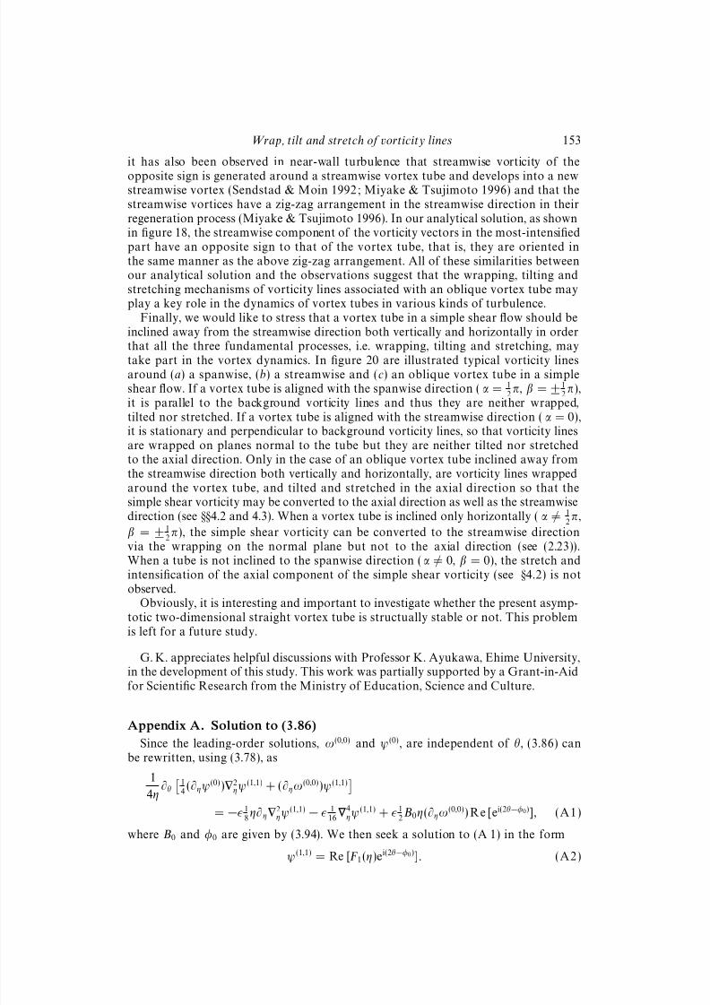
8/3/2019 Genta Kawahara et al- Wrap, tilt and stretch of vorticity lines around a strong thin straight vortex tube in a simple …
http://slidepdf.com/reader/full/genta-kawahara-et-al-wrap-tilt-and-stretch-of-vorticity-lines-around-a-strong 40/49
Wrap, tilt and stretch of vorticity lines 153
it has also been observed in near-wall turbulence that streamwise vorticity of the
opposite sign is generated around a streamwise vortex tube and develops into a newstreamwise vortex (Sendstad & Moin 1992; Miyake & Tsujimoto 1996) and that thestreamwise vortices have a zig-zag arrangement in the streamwise direction in theirregeneration process (Miyake & Tsujimoto 1996). In our analytical solution, as shownin figure 18, the streamwise component of the vorticity vectors in the most-intensifiedpart have an opposite sign to that of the vortex tube, that is, they are oriented inthe same manner as the above zig-zag arrangement. All of these similarities betweenour analytical solution and the observations suggest that the wrapping, tilting andstretching mechanisms of vorticity lines associated with an oblique vortex tube mayplay a key role in the dynamics of vortex tubes in various kinds of turbulence.
Finally, we would like to stress that a vortex tube in a simple shear flow should beinclined away from the streamwise direction both vertically and horizontally in order
that all the three fundamental processes, i.e. wrapping, tilting and stretching, maytake part in the vortex dynamics. In figure 20 are illustrated typical vorticity linesaround (a) a spanwise, (b) a streamwise and (c) an oblique vortex tube in a simpleshear flow. If a vortex tube is aligned with the spanwise direction (α = 1
2π, β = ± 1
2π),
it is parallel to the background vorticity lines and thus they are neither wrapped,tilted nor stretched. If a vortex tube is aligned with the streamwise direction (α = 0),it is stationary and perpendicular to background vorticity lines, so that vorticity linesare wrapped on planes normal to the tube but they are neither tilted nor stretchedto the axial direction. Only in the case of an oblique vortex tube inclined away fromthe streamwise direction both vertically and horizontally, are vorticity lines wrappedaround the vortex tube, and tilted and stretched in the axial direction so that thesimple shear vorticity may be converted to the axial direction as well as the streamwisedirection (see
§§4.2 and 4.3). When a vortex tube is inclined only horizontally ( α
= 1
2π,
β = ± 12 π), the simple shear vorticity can be converted to the streamwise direction
via the wrapping on the normal plane but not to the axial direction (see (2.23)).When a tube is not inclined to the spanwise direction (α = 0, β = 0), the stretch andintensification of the axial component of the simple shear vorticity (see §4.2) is notobserved.
Obviously, it is interesting and important to investigate whether the present asymp-totic two-dimensional straight vortex tube is structually stable or not. This problemis left for a future study.
G. K. appreciates helpful discussions with Professor K. Ayukawa, Ehime University,in the development of this study. This work was partially supported by a Grant-in-Aidfor Scientific Research from the Ministry of Education, Science and Culture.
Appendix A. Solution to (3.86)
Since the leading-order solutions, ω(0,0) and ψ(0), are independent of θ, (3.86) canbe rewritten, using (3.78), as
1
4η∂θ
14
(∂ηψ(0))2ηψ(1,1) + (∂ηω(0,0))ψ(1,1)
= − 1
8η∂η2
ηψ(1,1) − 116
4ηψ(1,1) + 1
2B0η(∂ηω(0,0))Re[ei(2θ−φ0)], (A1)
where B0 and φ0 are given by (3.94). We then seek a solution to (A 1) in the form
ψ(1,1) = Re [F 1(η)ei(2θ−φ0)]. (A2)
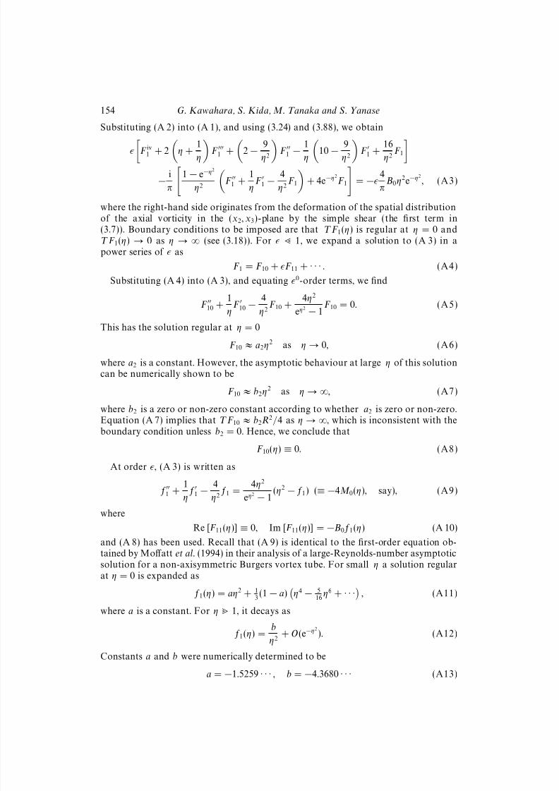
8/3/2019 Genta Kawahara et al- Wrap, tilt and stretch of vorticity lines around a strong thin straight vortex tube in a simple …
http://slidepdf.com/reader/full/genta-kawahara-et-al-wrap-tilt-and-stretch-of-vorticity-lines-around-a-strong 41/49
154 G. Kawahara, S. Kida, M. Tanaka and S. Yanase
Substituting (A 2) into (A 1), and using (3.24) and (3.88), we obtain
F iv1 + 2
η +1
η
F 1 +
2 − 9
η2
F 1 − 1
η
10 − 9
η2
F 1 +
16
η2F 1
− i
π
1 − e−η2
η2
F 1 +
1
ηF 1 − 4
η2F 1
+ 4e−η2
F 1
= −
4
πB0η2e−η2
, (A3)
where the right-hand side originates from the deformation of the spatial distributionof the axial vorticity in the (x2, x3)-plane by the simple shear (the first term in(3.7)). Boundary conditions to be imposed are that T F 1(η) is regular at η = 0 andT F 1(η) → 0 as η → ∞ (see (3.18)). For 1, we expand a solution to (A 3) in apower series of as
F 1 = F 10 + F 11 +
· · ·. (A4)
Substituting (A 4) into (A 3), and equating 0-order terms, we find
F 10 +1
ηF 10 − 4
η2F 10 +
4η2
eη2 − 1F 10 = 0. (A5)
This has the solution regular at η = 0
F 10 ≈ a2η2 as η → 0, (A6)
where a2 is a constant. However, the asymptotic behaviour at large η of this solutioncan be numerically shown to be
F 10 ≈ b2η2 as η → ∞, (A7)
where b2 is a zero or non-zero constant according to whether a2 is zero or non-zero.Equation (A 7) implies that T F 10 ≈ b2R2/4 as η → ∞, which is inconsistent with theboundary condition unless b2 = 0. Hence, we conclude that
F 10(η) ≡ 0. (A8)
At order , (A 3) is written as
f1 +
1
η f
1 − 4
η2 f1 =
4η2
eη2 − 1(η2 − f1) (≡ −4M 0(η), say), (A9)
where
Re [F 11(η)] ≡ 0, Im [F 11(η)] = −B0 f1(η) (A 10)
and (A 8) has been used. Recall that (A 9) is identical to the first-order equation ob-
tained by Moffatt et al. (1994) in their analysis of a large-Reynolds-number asymptoticsolution for a non-axisymmetric Burgers vortex tube. For small η a solution regularat η = 0 is expanded as
f1(η) = aη2 + 13
(1 − a)
η4 − 516
η6 + · · · , (A11)
where a is a constant. For η 1, it decays as
f1(η) =b
η2+ O(e−η2
). (A12)
Constants a and b were numerically determined to be
a = −1.5259 · · · , b = −4.3680 · · · (A13)
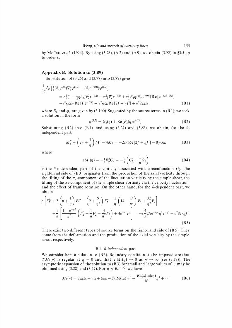
8/3/2019 Genta Kawahara et al- Wrap, tilt and stretch of vorticity lines around a strong thin straight vortex tube in a simple …
http://slidepdf.com/reader/full/genta-kawahara-et-al-wrap-tilt-and-stretch-of-vorticity-lines-around-a-strong 42/49
Wrap, tilt and stretch of vorticity lines 155
by Moffatt et al. (1994). By using (3.78), (A 2) and (A 9), we obtain (3.92) in
§3.5 up
to order .
Appendix B. Solution to (3.89)
Substitution of (3.25) and (3.78) into (3.89) gives
1
4η∂θ
14
(∂ηψ(0))2ηψ(1,2) + (∂ηω(0,0))ψ(1,2)
= 1
4(1 − 1
2η∂η)2
ηψ(1,2) − 116
4ηψ(1,2) + 1
2B1η(∂ηω(0,0))Re[e−i(2θ−φ1)]
−2 12
ξ0η Re [ fe−i2θ] + 2 12
ξ0 Re[2 f + ηf ] + 22γ0λ0, (B1)
where B1 and φ1 are given by (3.100). Suggested by the source terms in (B 1), we seek
a solution in the form
ψ(1,2) = G2(η) + Re [F 2(η)e−i2θ]. (B2)
Substituting (B 2) into (B 1), and using (3.24) and (3.88), we obtain, for the θ-independent part,
M 1 +
2η +
1
η
M 1 − 4M 1 = −2ξ0 Re[2 f + ηf ] − 8γ0λ0, (B3)
where
M 1(η) = − 142
ηG2 = − 14
G
2 +1
ηG
2
(B4)
is the θ-independent part of the vorticity associated with streamfunction G2. The
right-hand side of (B 3) originates from the production of the axial vorticity throughthe tilting of the x2-component of the fluctuation vorticity by the simple shear, thetilting of the x3-component of the simple shear vorticity via the velocity fluctuation,and the effect of frame rotation. On the other hand, for the θ-dependent part, weobtain
F iv2 + 2
η +
1
η
F 2 −
2 +
9
η2
F 2 − 1
η
14 − 9
η2
F 2 +
32
η2F 2
+
i
π
1 − e−η2
η2
F 2 +
1
ηF 2 − 4
η2F 2
+ 4e−η2
F 2
= −
4
πB1e−iφ1 η2e−η2 − 28ξ0ηf .
(B5)
There exist two different types of source terms on the right-hand side of (B 5). Theycome from the deformation and the production of the axial vorticity by the simpleshear, respectively.
B.1. θ-independent part
We consider here a solution to (B 3). Boundary conditions to be imposed are thatT M 1(η) is regular at η = 0 and that T M 1(η) → 0 as η → ∞ (see (3.17)). Theasymptotic expansion of the solution to (B 3) for small and large values of η may beobtained using (3.28) and (3.27). For η Re−1/2, we have
M 1(η) = 2γ0λ0 + m0 + (m0 − ξ0Re(c0))η2 − Reξ0Im(c0)
16η4 + · · · (B6)
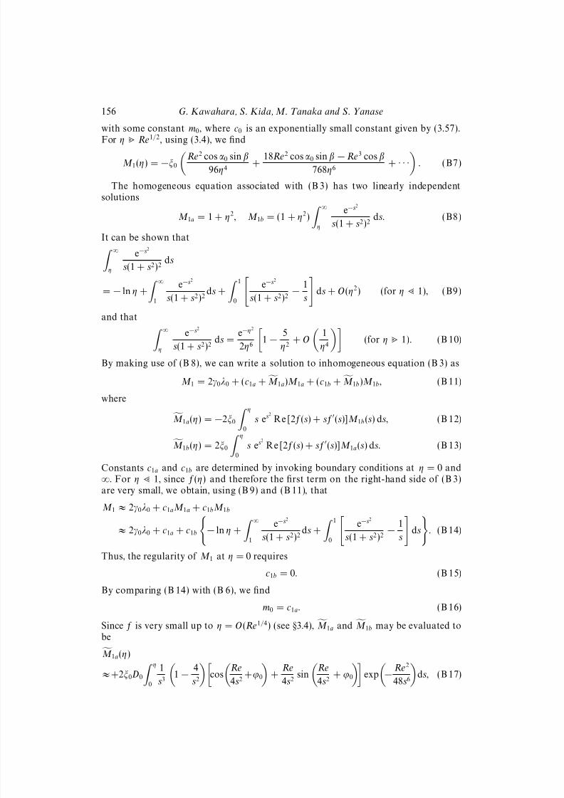
8/3/2019 Genta Kawahara et al- Wrap, tilt and stretch of vorticity lines around a strong thin straight vortex tube in a simple …
http://slidepdf.com/reader/full/genta-kawahara-et-al-wrap-tilt-and-stretch-of-vorticity-lines-around-a-strong 43/49
8/3/2019 Genta Kawahara et al- Wrap, tilt and stretch of vorticity lines around a strong thin straight vortex tube in a simple …
http://slidepdf.com/reader/full/genta-kawahara-et-al-wrap-tilt-and-stretch-of-vorticity-lines-around-a-strong 44/49
Wrap, tilt and stretch of vorticity lines 157
M 1b(η)
≈−4ξ0D0 η
0
s31 +1
s2
cosRe4s2
+ ϕ0+
Re4s2
sinRe4s2
+ ϕ0 exps2 − Re2
48s6
ds (B 18)
by using (3.63), (3.64), (B 8) and (B 10). After elementary calculation, we arrive at
M 1a(η) ≈ −ξ0D0
8
Re
sin
Re
4η2+ ϕ0
− Re
8η2cos
Re
4η2+ ϕ0
− 16
Re2
Re2
16η4+ 2
cos
Re
4η2+ ϕ0
+
Re
4η2
Re2
16η4+ 2
sin
Re
4η2+ ϕ0
+ · · ·
exp
− Re2
48η6
, (B 19)
M 1b(η) ≈ −ξ0D0η2 2cos Re
4η2+ ϕ0
+ Re2η2
sin Re4η2
+ ϕ0 exp− Re2
48η6
+
4 − Re2
8η4
cos
Re
4η2+ ϕ0
+
Re
η2sin
Re
4η2+ ϕ0
exp
− Re2
48η6
+ · · ·
eη2
. (B 20)
For η Re1/2, (B 19) and (B 20) are reduced to
M 1a(η) ≈−ξ0D0
8sin ϕ0
Re− 32 cos ϕ0
Re2+
cos ϕ0
η2− 2cos ϕ0
η4+
Re2 cos ϕ0
96η6+ · · ·
, (B 21)
M 1b(η) ≈ −2ξ0D0η2eη2
cos ϕ0 +
2cos ϕ0
η2+
Re2 cos ϕ0
32η4+ · · ·
. (B 22)
Then, M 1aM 1a and M 1bM 1b can be written, using (B 8), (B 10), (B 21) and (B 22), as
M 1aM 1a ≈−ξ0D0
8sin ϕ0
Re[1+ O(Re−1)](1+η2)+cos ϕ0 − cos ϕ0
η2+
Re2 cos ϕ0
96η4
, (B 23)
M 1bM 1b ≈ −ξ0D0
cos ϕ0
η2. (B 24)
It follows from (3.4), (B 8), (B 10), (B 11), (B 15), (B 23) and (B 24) that
M 1 ≈c1a − 8ξ0 cos β
Re+O(Re−2)
(1+ η2) − ξ0Re2 cos α0 sin β
96η4(for η Re1/2). (B 25)
Since M 1(η) must approach zero as η → ∞, we find
m0 = c1a ≈ 8ξ0 cos βRe
. (B 26)
Then the last term in (B 25) gives the leading order, which is consistent with theleading term in asymptotic expansion (B 7). Equations (B 8), (B 11), (B 17) and (B 18)provide a solution to (B 3) for given constants c1a and c1b.
Consider now an asymptotic form of M 1(η) at large Reynolds numbers. Forη . Re1/4, the first term on the right-hand side of (B 3) is very small, and so using(B 15) we have
M 1 ≈ 2γ0λ0 + c1aM 1a ≈ 2γ0λ0 +8ξ0 cos βη 2
Re. (B 27)
For η Re1/4, on the other hand, (B 8), (B 10), (B 19) and (B 20) give asymptotic

8/3/2019 Genta Kawahara et al- Wrap, tilt and stretch of vorticity lines around a strong thin straight vortex tube in a simple …
http://slidepdf.com/reader/full/genta-kawahara-et-al-wrap-tilt-and-stretch-of-vorticity-lines-around-a-strong 45/49
158 G. Kawahara, S. Kida, M. Tanaka and S. Yanase
forms of M 1aM 1a and M 1bM 1b as
M 1aM 1a ≈ −ξ0D0
8η2
Resin Re
4η2+ ϕ0
− cos Re
4η2+ ϕ0
exp
− Re2
48η6
, (B 28)
M 1bM 1b ≈ −ξ0D0
1
η2cos
Re
4η2+ ϕ0
+
Re
4η4sin
Re
4η2+ ϕ0
exp
− Re2
48η6
. (B 29)
Since M 1aM 1a M 1bM 1b for η Re1/4, we can express an asymptotic form of M 1(η)
for η Re1/4, using (B 11), (B 26) and (B 28), as (3.98) in §3.5. Equation (3.98) matches(B 27) for η Re1/3, and thus (3.98) turns out to be available for any value of η.
B.2. θ-dependent part with zero mean
Solutions to (B 5) are considered here. Boundary conditions to be imposed are thatT 2F 2(η) is regular at η = 0 and that T 2F 2(η) → 0 as η → ∞ (see (3.18)). Twosource terms on the right-hand side of (B 5) have peak values at extremely differentlocations for Re 1. The first term has a peak value of O(Re−1) at η = 1 and rapidlydecreases as η increases. The second is, on the other hand, exponentially small up toη = O(Re1/4), and it has a peak value of O(Re−5/3) at η = 2−2/3Re1/3 (see §3.4). Hence,for Re 1, we consider two regions of values of η separately, that is, η = O(1) andη 1.
First, in the region η = O(1) we take only the first term on the right-hand side of (B 5). By substituting an -expansion,
F 2 = F 20 + F 21 + · · · (B 30)
into (B 5), we obtain, at order 0,
F 20 +1
ηF 20 − 4
η2F 20 +
4η2
eη2 − 1F 20 = 0, (B 31)
which is the same as (A 5), and therefore
F 20(η) ≡ 0. (B 32)
At order of (B 5), by putting
F 21(η) = iB1e−iφ1 f2(η), (B 33)
we obtain
f2 +
1
η
f2
−4
η
2 f2 =
4η2
e
η2
− 1
(η2
− f2), (B 34)
which is identical to (A 9). Hence, we can take
Re[ f2(η)] ≡ f1(η), Im[ f2(η)] ≡ 0, (B 35)
so that
F 21(η) = iB1e−iφ1 f1(η). (B 36)
Combination of (A 9), (B 30), (B 32) and (B 36) leads to the first equation of (3.99) in§3.5.
By introducing
M 2(η) = − 14
F 2 +
1
ηF 2 − 4
η2F 2
(B 37)
8/3/2019 Genta Kawahara et al- Wrap, tilt and stretch of vorticity lines around a strong thin straight vortex tube in a simple …
http://slidepdf.com/reader/full/genta-kawahara-et-al-wrap-tilt-and-stretch-of-vorticity-lines-around-a-strong 46/49
Wrap, tilt and stretch of vorticity lines 159
and using (3.78) we may express the θ-dependent part of vorticity associated with
streamfunction Re [F 2(η)e−i2θ] as
− 142
ηRe [F 2(η)e−i2θ] = Re [M 2(η)e−i2θ]. (B 38)
Second, we consider the region η 1 in which all the terms that include e−η2
maybe neglected. By dropping them and using (B 37), we can rewrite (B 5) as
M 2 +
2η +
1
η
M 2 + 2
iRe − 2
η2− 2
M 2 = 2ξ0ηf . (B 39)
Boundary conditions to be imposed are that T M 2(η) is regular at η = 0 and thatT M 2(η) → 0 as η → ∞ (see (3.17)). Using (3.28) and (3.27), we can expand a solutionto (B 39) as
M 2(η) = −ξ0c0 iRe
4(iRe + 6) η4 −24iRe + (iRe + 6)(8iRe
−Re2)
48(iRe + 6)(iRe + 16) η6 + · · ·(for η Re−1/2), (B 40)
and
M 2(η) = −ξ0D0eiϕ0
iRe
8η2− Re2
24η4− (11iRe + 72)Re2
1536η6+ · · ·
(for η Re1/2),
(B 41)where c0 is an exponentially small constant given by (3.57).
Now, following the asymptotic analysis performed for (3.26) in §3.4, we employ theWKB method in order to construct solutions to the homogeneous equation associatedwith (B 39). Let us introduce a new dependent variable g2(η) by
M 2(η) = η−1/2e−η2
/2g2(η). (B 42)
By substituting (B 42) into (B 39), we obtain
g2 +
2iRe
η2− η2 − 6 − 15
4η2
g2 = 2ξ0η3/2eη2/2 f. (B 43)
We consider the region η = O(Re1/4) and put η = Re1/4χ. Then, (B 43) becomes
g2 + Re
2i
χ2− χ2 − 6Re−1/2 + O(Re−1)
g2 = 2Re3/4ξ0χ3/2 exp
12
Re1/2χ2
f. (B 44)
The homogeneous equation associated with (B 44) has two linearly independent WKBsolutions
g2a = χ1/2(χ4 − 2i)−1/4 χ2 + (χ4 − 2i)1/2−3/2 exp −Re1/2σ1(χ) , (B 45)
g2b = χ1/2(χ4 − 2i)−1/4
χ2 + (χ4 − 2i)1/23/2
exp
Re1/2σ1(χ)
, (B 46)
where
σ1(χ) = 2−1/2eπi/4
e−πi/4( 12
χ4 − i)1/2 − arctan
e−πi/4( 12
χ4 − i)1/2
+ 12
π
. (B 47)
For small values of χ, function σ1(χ) may be expressed asymptotically as
σ1 =√
2e−πi/4 ln χ + ρ1 + O(χ4), (B 48)
where
ρ1 = 32
2−1/2e3πi/4 ln2 + 12
14
π + 1 + i
14
π − 1
. (B 49)
8/3/2019 Genta Kawahara et al- Wrap, tilt and stretch of vorticity lines around a strong thin straight vortex tube in a simple …
http://slidepdf.com/reader/full/genta-kawahara-et-al-wrap-tilt-and-stretch-of-vorticity-lines-around-a-strong 47/49
160 G. Kawahara, S. Kida, M. Tanaka and S. Yanase
For large χ, on the other hand, it is expanded as
σ1 = 12
χ2 +i
2χ2− 1
12χ6+ · · · . (B 50)
Then, we use (B 48) and (B 50), and restore the original variable η to obtain, forη Re1/4 (χ 1),
g2a(η) ≈ Re−1/82−1η1/2 exp−Re1/2(
√ 2e−πi/4 ln η +
√ 2e3πi/4 ln Re1/4 + ρ1)
, (B 51)
g2b(η) ≈ Re−1/8√ 2e−πi/4η1/2 exp
Re1/2(
√ 2e−πi/4 ln η +
√ 2e3πi/4 ln Re1/4 + ρ1)
, (B 52)
and, for η Re1/4 (χ 1),
g2a(η)
≈2−3/2Re7/8η−7/2 exp−
12
η2
−iRe
2η2
+Re2
12η6 , (B 53)
g2b(η) ≈ 23/2Re−5/8η5/2 exp
12
η2 +iRe
2η2− Re2
12η6
. (B 54)
In order to solve the full equation (B 44), we write a solution in terms of (B 45) and(B 46) as
g2(η) = (c2a + g2a(η))g2a(η) + (c2b + g2b(η))g2b(η), (B 55)
where
g2a(η) = −2ξ0
η
0
s3/2e1/2s2
f(s)g2b(s)
W (s)ds, (B 56)
g2b(η) =
−2ξ0
∞
η
s3/2e1/2s2
f(s)g2a(s)
W (s)ds, (B 57)
with
W (η) = g2a(η)g2b(η) − g
2a(η)g2b(η). (B 58)
It can be shown from (B 51)–(B 54) that
W (η) ≈ 2Re1/4. (B 59)
Constants c2a and c2b are determined by the boundary conditions at η = 0 and ∞.For η Re1/4, since f(η) and therefore the right-hand side of (B 44) are very small,(B 55) is written, using (B 51) and (B 52), as
g2 ≈ c2ag2a + c2bg2b ≈ c2a2−1Re−1/8eπi/2q−11 η−q2+ 1
2 + c2b
√ 2Re−1/8e−πi/4q1ηq2+ 1
2 , (B 60)
whereq1 = exp
Re1/2(
√ 2e3πi/4 ln Re1/4 + ρ1)
, (B 61)
q2 = Re1/2√ 2e−πi/4. (B 62)
Since Re (q2) = Re1/2, and q1 is exponentially small for Re 1, we obtain, usingdefinition (B 42) of g2,
M 2 ≈ c2a2−1Re−1/8q−11 η−q2 (at η Re1/4). (B 63)
Hence, in order that M 2 may be connected smoothly with a regular solution at η = 0we must take
c2a = 0. (B 64)
8/3/2019 Genta Kawahara et al- Wrap, tilt and stretch of vorticity lines around a strong thin straight vortex tube in a simple …
http://slidepdf.com/reader/full/genta-kawahara-et-al-wrap-tilt-and-stretch-of-vorticity-lines-around-a-strong 48/49
Wrap, tilt and stretch of vorticity lines 161
For η Re1/4, it can be shown by using (3.64), (B 53) and (B 54) that
g2a ≈ −i√
2ξ0D0eiϕ0 Re1/8 η
0
s exp
s2 +3iRe
4s2− 5Re2
48s6
ds, (B 65)
g2b ≈ −i2−5/2ξ0D0eiϕ0 Re13/8
∞η
1
s5exp
− iRe
4s2+
Re2
16s6
ds (B 66)
because f is very small up to η = O(Re1/4) (see §3.4). Integrations by parts of theintegrals in (B 65) and (B 66) respectively lead to
g2a ≈ −i2−1/2ξ0D0eiϕ0 Re1/8 exp
η2 +
3iRe
4η2− 5Re2
48η6
, (B 67)
g2b ≈ −i√ 2ξ0D0eiϕ0
Re−3/8 1 +
iRe
4η2 exp−iRe
4η2 +
Re2
16η6− 1 . (B 68)
Thus, it follows from (B 42), (B 53)–(B 55), (B 64), (B 67) and (B 68) that
M 2(η) ≈ c2b23/2Re−5/8η2 exp
iRe
2η2− Re2
12η6
−iξ0D0eiϕ0
4η2
Re
1 +
iRe
4η2
exp
iRe
4η2− Re2
48η6
− exp
iRe
2η2− Re2
12η6
−iξ0D0eiϕ0
Re
4η4exp
iRe
4η2− Re2
48η6
. (B 69)
Furthermore, for η Re1/2, we expand (B 69) in a series of inverse powers of η to
obtainM 2 ≈ c2b23/2Re−5/8η2 − ξ0D0eiϕ0
iRe
8η2. (B 70)
Function M 2(η) must vanish as η → ∞. This requires that
c2b = 0, (B 71)
and then the last term in (B 70) gives the leading order, which is consistent with theleading term in asymptotic expansion (B 41). Given constants c2a and c2b, then (B 55),(B 65) and (B 66) provide a solution to (B 44), and M 2(η) is determined by (B 42).
Let us summarize an asymptotic form of M 2(η) at a large Reynolds number. For1 η . Re1/4, the right-hand side of (B 39) is very small, and so is M 2(η) becausec2a = c2b = 0. For η Re1/4, on the other hand, the second term on the left-hand
side of (B 69) dominates the third (the first term has already vanished), and then anasymptotic form of M 2(η) is given by the second equation of (3.99) in §3.5.
REFERENCES
Bernard, P. S., Thomas, J. M. & Handler, R. A. 1993 Vortex dynamics and the production of Reynolds stress. J. Fluid Mech. 253, 385–419.
Brooke, J. W. & Hanratty, T. J. 1993 Origin of turbulence-producing eddies in a channel flow.Phys. Fluids A 5, 1011–1022.
Choi, H., Moin, P. & Kim, J. 1993 Direct numerical simulation of turbulent flow over riblets. J.Fluid Mech. 255, 503–539.
Douady, D., Couder, Y. & Brachet, M. E. 1991 Direct observation of the intermittency of intensevorticity filaments in turbulence. Phys. Rev. Lett. 67, 983–986.
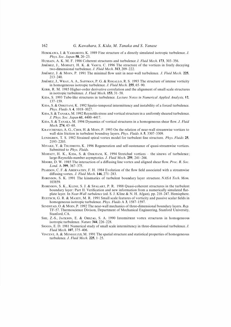
8/3/2019 Genta Kawahara et al- Wrap, tilt and stretch of vorticity lines around a strong thin straight vortex tube in a simple …
http://slidepdf.com/reader/full/genta-kawahara-et-al-wrap-tilt-and-stretch-of-vorticity-lines-around-a-strong 49/49
162 G. Kawahara, S. Kida, M. Tanaka and S. Yanase
Hosokawa, I. & Yamamoto, K. 1989 Fine structure of a directly simulated isotropic turbulence. J.
Phys. Soc. Japan 58, 20–23.Hussain, A. K. M. F. 1986 Coherent structures and turbulence J. Fluid Mech. 173, 303–356.
Jimemez, J., Moffatt, H. K. & Vasco, C. 1996 The structure of the vortices in freely decayingtwo-dimensional turbulence. J. Fluid Mech. 313, 209–222.
Jimemez, J. & Moin, P. 1991 The minimal flow unit in near-wall turbulence. J. Fluid Mech. 225,213–240.
Jimemez, J., Wray, A. A., Saffman, P. G. & Rogallo, R. S. 1993 The structure of intense vorticityin homogeneous isotropic turbulence. J. Fluid Mech. 255, 65–90.
Kerr, R. M. 1985 Higher-order derivative correlation and the alignment of small scale structuresin isotropic turbulence. J. Fluid Mech. 153, 31–58.
Kida, S. 1993 Tube-like structures in turbulence. Lecture Notes in Numerical Applied Analysis, 12,137–159.
Kida, S. & Ohkitani, K. 1992 Spatio-temporal intermittency and instability of a forced turbulence.Phys. Fluids A 4, 1018–1027.
Kida, S. & Tanaka, M. 1992 Reynolds stress and vortical structure in a uniformly sheared turbulence.J. Phys. Soc. Japan 61, 4400–4417.Kida, S. & Tanaka, M. 1994 Dynamics of vortical structures in a homogeneous shear flow. J. Fluid
Mech. 274, 43–68.
Kravchenko, A. G., Choi, H. & Moin, P. 1993 On the relation of near-wall streamwise vortices towall skin friction in turbulent boundray layers. Phys. Fluids A 5, 3307–3309.
Lundgren, T. S. 1982 Strained spiral vortex model for turbulent fine structure. Phys. Fluids 25,2193–2203.
Miyake, Y. & Tsujimoto, K. 1996 Regeneration and self-sustenance of quasi-streamwise vortices.Submitted to Phys. Fluids.
Moffatt, H. K., Kida, S. & Ohkitani, K. 1994 Stretched vortices – the sinews of turbulence;large-Reynolds-number asymptotics. J. Fluid Mech. 259, 241–264.
Moore, D. W. 1985 The interaction of a diffusing line vortex and aligned shear flow. Proc. R. Soc.Lond. A 399, 367–375.
Pearson, C. F. & Abernathy, F. H. 1984 Evolution of the flow field associated with a streamwisediffusing vortex. J. Fluid Mech. 146, 271–283.
Robinson, S. K. 1991 The kinematics of turbulent boundary layer structure. NASA Tech. Mem.103859.
Robinson, S. K., Kline, S. J. & Spalart, P. R. 1988 Quasi-coherent structures in the turbulentboundary layer: Part II. Verification and new information from a numerically simulated flat-plate layer. In Near-Wall turbulence (ed. S. J. Kline & N. H. Afgan), pp. 218–247. Hemisphere.
Ruetsch, G. R. & Maxey, M. R. 1991 Small scale features of vorticity and passive scalar fields inhomogeneous isotropic turbulence. Phys. Fluids A 3, 1587–1597.
Sendstad, O. & Moin, P. 1992 The near-wall mechanics of three-dimensional boundary layers. Rep.TF-57. Thermoscience Divison, Department of Mechanical Engineering, Stanford University,Stanford, CA.
She, Z.-S., Jackson, E. & Orszag, S. A. 1990 Intermittent vortex structures in homogeneousisotropic turbulence. Nature 344, 226–228.
Siggia, E. D. 1981 Numerical study of small scale intermittency in three-dimensional turbulence. J.
Fluid Mech. 107, 375–406.Vincent, A. & Meneguzzi, M. 1991 The spatial structure and statistical properties of homogeneous
turbulence. J. Fluid Mech. 225, 1–25.