Embed Size (px)
Citation preview
The problem Mixing in isopycnal coordinates Summary Discussion questions References
The Gent-McWilliamsparameterization of eddy
buoyancy fluxes
(as told by Cesar)
slides at tinyurl.com/POTheory-GM
Gent & McWilliams, JPO, 1990 Griffies, JPO, 1998(The most cited JPO paper ?)
PO theory seminar, SIO, fall 2016 The Gent-McWilliams parameterization

The problem Mixing in isopycnal coordinates Summary Discussion questions References
Climate models are devoid of mesoscale eddiesIn 1990, ocean models had “coarse resolution” (many still do today)
Source: Hallberg & Gnanadesikan.
PO theory seminar, SIO, fall 2016 The Gent-McWilliams parameterization

The problem Mixing in isopycnal coordinates Summary Discussion questions References
A stroll through GM
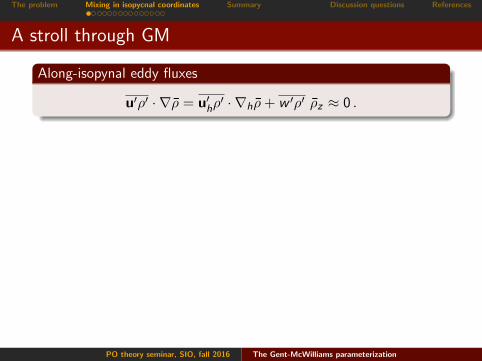
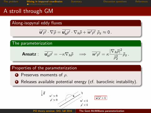
Along-isopynal eddy fluxes
u′ρ′ · ∇ρ = u′hρ′ · ∇hρ+ w ′ρ′ ρz ≈ 0 .
The parameterization
Ansatz : u′hρ′ = −κ∇hρ =⇒ w ′ρ′ = κ
|∇hρ|2
ρ2z
ρz .
Properties of the parameterization
1 Preserves moments of ρ.
2 Releases available potential energy (cf. baroclinic instability).
PO theory seminar, SIO, fall 2016 The Gent-McWilliams parameterization
The problem Mixing in isopycnal coordinates Summary Discussion questions References
A stroll through GM
Along-isopynal eddy fluxes
u′ρ′ · ∇ρ = u′hρ′ · ∇hρ+ w ′ρ′ ρz ≈ 0 .
The parameterization
Ansatz : u′hρ′ = −κ∇hρ =⇒ w ′ρ′ = κ
|∇hρ|2
ρ2z
ρz .
Properties of the parameterization
1 Preserves moments of ρ.
2 Releases available potential energy (cf. baroclinic instability).
PO theory seminar, SIO, fall 2016 The Gent-McWilliams parameterization

The problem Mixing in isopycnal coordinates Summary Discussion questions References
Density (buoyancy) coordinates
f (x , y , z , t) = f (x , y , ρ, t) , fx = fx+ρx fρ , fz = ρz fρ , · · ·
(cf. Young, JPO, 2012.)
PO theory seminar, SIO, fall 2016 The Gent-McWilliams parameterization
The problem Mixing in isopycnal coordinates Summary Discussion questions References
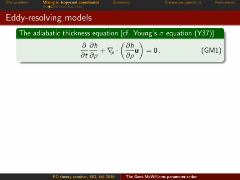
Eddy-resolving models
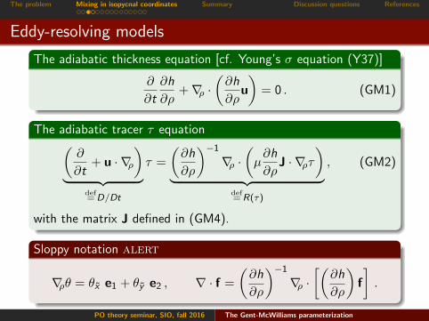
The adiabatic thickness equation [cf. Young’s σ equation (Y37)]
∂
∂t
∂h
∂ρ+∇ρ ·
(∂h
∂ρu
)= 0 . (GM1)
The adiabatic tracer τ equation(∂
∂t+ u · ∇ρ
)︸ ︷︷ ︸
def= D/Dt
τ =
(∂h
∂ρ
)−1
∇ρ ·(µ∂h
∂ρJ · ∇ρτ
)︸ ︷︷ ︸
def= R(τ)
, (GM2)
with the matrix J defined in (GM4).
Sloppy notation alert
∇ρθ = θx e1 + θy e2 , ∇ · f =
(∂h
∂ρ
)−1
∇ρ ·[(
∂h
∂ρ
)f
].
PO theory seminar, SIO, fall 2016 The Gent-McWilliams parameterization

The problem Mixing in isopycnal coordinates Summary Discussion questions References
Eddy-resolving models
The adiabatic thickness equation [cf. Young’s σ equation (Y37)]
∂
∂t
∂h
∂ρ+∇ρ ·
(∂h
∂ρu
)= 0 . (GM1)
The adiabatic tracer τ equation(∂
∂t+ u · ∇ρ
)︸ ︷︷ ︸
def= D/Dt
τ =
(∂h
∂ρ
)−1
∇ρ ·(µ∂h
∂ρJ · ∇ρτ
)︸ ︷︷ ︸
def= R(τ)
, (GM2)
with the matrix J defined in (GM4).
Sloppy notation alert
∇ρθ = θx e1 + θy e2 , ∇ · f =
(∂h
∂ρ
)−1
∇ρ ·[(
∂h
∂ρ
)f
].
PO theory seminar, SIO, fall 2016 The Gent-McWilliams parameterization

The problem Mixing in isopycnal coordinates Summary Discussion questions References
Eddy-resolving models
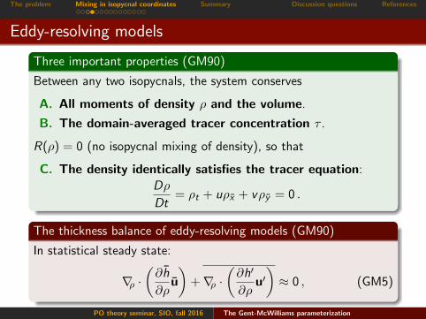
Three important properties (GM90)
Between any two isopycnals, the system conserves
A. All moments of density ρ and the volume.
B. The domain-averaged tracer concentration τ .
R(ρ) = 0 (no isopycnal mixing of density), so that
C. The density identically satisfies the tracer equation:
Dρ
Dt= ρt + uρx + vρy = 0 .
The thickness balance of eddy-resolving models (GM90)
In statistical steady state:
∇ρ ·(∂h
∂ρu
)+∇ρ ·
(∂h′
∂ρu′)≈ 0 , (GM5)
PO theory seminar, SIO, fall 2016 The Gent-McWilliams parameterization
The problem Mixing in isopycnal coordinates Summary Discussion questions References
Eddy-resolving models
Three important properties (GM90)
Between any two isopycnals, the system conserves
A. All moments of density ρ and the volume.
B. The domain-averaged tracer concentration τ .
R(ρ) = 0 (no isopycnal mixing of density), so that
C. The density identically satisfies the tracer equation:
Dρ
Dt= ρt + uρx + vρy = 0 .
The thickness balance of eddy-resolving models (GM90)
In statistical steady state:
∇ρ ·(∂h
∂ρu
)+∇ρ ·
(∂h′
∂ρu′)≈ 0 , (GM5)
PO theory seminar, SIO, fall 2016 The Gent-McWilliams parameterization
The problem Mixing in isopycnal coordinates Summary Discussion questions References
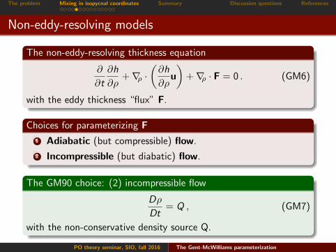
Non-eddy-resolving models
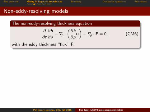
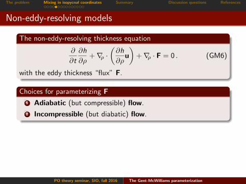
The non-eddy-resolving thickness equation
∂
∂t
∂h
∂ρ+∇ρ ·
(∂h
∂ρu
)+∇ρ · F = 0 . (GM6)
with the eddy thickness “flux” F.
Choices for parameterizing F
1 Adiabatic (but compressible) flow.
2 Incompressible (but diabatic) flow.
The GM90 choice: (2) incompressible flow
Dρ
Dt= Q , (GM7)
with the non-conservative density source Q.
PO theory seminar, SIO, fall 2016 The Gent-McWilliams parameterization
The problem Mixing in isopycnal coordinates Summary Discussion questions References
Non-eddy-resolving models
The non-eddy-resolving thickness equation
∂
∂t
∂h
∂ρ+∇ρ ·
(∂h
∂ρu
)+∇ρ · F = 0 . (GM6)
with the eddy thickness “flux” F.
Choices for parameterizing F
1 Adiabatic (but compressible) flow.
2 Incompressible (but diabatic) flow.
The GM90 choice: (2) incompressible flow
Dρ
Dt= Q , (GM7)
with the non-conservative density source Q.
PO theory seminar, SIO, fall 2016 The Gent-McWilliams parameterization
The problem Mixing in isopycnal coordinates Summary Discussion questions References
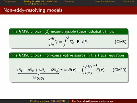
Non-eddy-resolving models
The GM90 choice: (2) incompressible (quasi-adiabatic) flow
∂h
∂ρQ =
∫ ρ
∇ρ · F dρ . (GM8)
The GM90 choice: non-conservative source in the tracer equation
(∂t + u∂x + v∂y + Q∂ρ)︸ ︷︷ ︸def= D/Dt
τ = R(τ) +
(∂h
∂ρ
)−1
E (τ) . (GM10)
PO theory seminar, SIO, fall 2016 The Gent-McWilliams parameterization
The problem Mixing in isopycnal coordinates Summary Discussion questions References
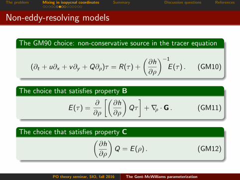
Non-eddy-resolving models
The GM90 choice: non-conservative source in the tracer equation
(∂t + u∂x + v∂y + Q∂ρ)τ = R(τ) +
(∂h
∂ρ
)−1
E (τ) . (GM10)
The choice that satisfies property B
E (τ) =∂
∂ρ
[(∂h
∂ρ
)Qτ
]+∇ρ · G . (GM11)
The choice that satisfies property C(∂h
∂ρ
)Q = E (ρ) . (GM12)
PO theory seminar, SIO, fall 2016 The Gent-McWilliams parameterization

The problem Mixing in isopycnal coordinates Summary Discussion questions References
Non-eddy-resolving models
The “flux” G satisfy
∇ρ · [ρF + G(ρ)] = 0 , (GM13)
so that the simplest solution is
G(τ) = −τF .
The non-eddy-resolving tracer equation
(∂t + u · ∇ρ) τ +
(∂h
∂ρ
)−1
F︸ ︷︷ ︸Eddy velocity
·∇ρτ = R(τ) . (GM14)
Recall: F =(∂h∂ρ
)′u′.
PO theory seminar, SIO, fall 2016 The Gent-McWilliams parameterization
The problem Mixing in isopycnal coordinates Summary Discussion questions References
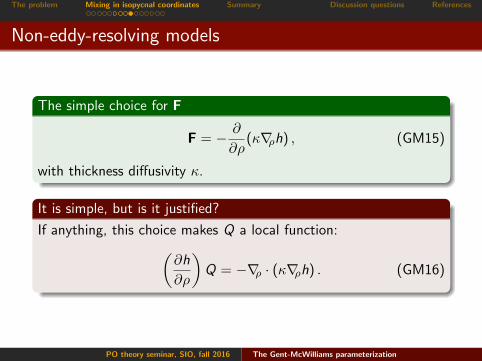
Non-eddy-resolving models
The simple choice for F
F = − ∂
∂ρ(κ∇ρh) , (GM15)
with thickness diffusivity κ.
It is simple, but is it justified?
If anything, this choice makes Q a local function:(∂h
∂ρ
)Q = −∇ρ · (κ∇ρh) . (GM16)
PO theory seminar, SIO, fall 2016 The Gent-McWilliams parameterization
The problem Mixing in isopycnal coordinates Summary Discussion questions References
The GM skew flux
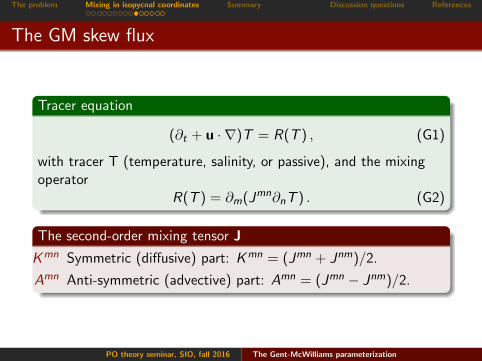
Tracer equation
(∂t + u · ∇)T = R(T ) , (G1)
with tracer T (temperature, salinity, or passive), and the mixingoperator
R(T ) = ∂m(Jmn∂nT ) . (G2)
The second-order mixing tensor J
Kmn Symmetric (diffusive) part: Kmn = (Jmn + Jnm)/2.
Amn Anti-symmetric (advective) part: Amn = (Jmn − Jnm)/2.
PO theory seminar, SIO, fall 2016 The Gent-McWilliams parameterization

The problem Mixing in isopycnal coordinates Summary Discussion questions References
The GM skew flux
Two forms of the stirring operator
RA(T ) = ∂m(Amn∂nT︸ ︷︷ ︸def=−Fm
skew
) = (∂mAmn)∂nT +���
���:0
Amn∂n∂mT (G7)
= ∂n[(∂mAmn)T︸ ︷︷ ︸
def=−F n
adv
]−������:
0T∂m∂nA
mn (G3)
PO theory seminar, SIO, fall 2016 The Gent-McWilliams parameterization
The problem Mixing in isopycnal coordinates Summary Discussion questions References
The GM skew flux
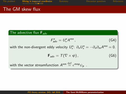
The advective flux Fadv
F nadv = Un
?Amn , (G4)
with the non-divergent eddy velocity Un? : ∂nU
n? = −∂n∂mAmn = 0.
Fadv = T (∇×ψ) , (G6)
with the vector streamfunction Anm def= εmnpψp .
PO theory seminar, SIO, fall 2016 The Gent-McWilliams parameterization
The problem Mixing in isopycnal coordinates Summary Discussion questions References
The GM skew flux
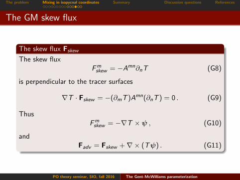
The skew flux Fskew
The skew fluxFmskew = −Amn∂nT (G8)
is perpendicular to the tracer surfaces
∇T · Fskew = −(∂mT )Amn(∂nT ) = 0 . (G9)
ThusFmskew = −∇T ×ψ , (G10)
andFadv = Fskew +∇× (Tψ) . (G11)
PO theory seminar, SIO, fall 2016 The Gent-McWilliams parameterization
The problem Mixing in isopycnal coordinates Summary Discussion questions References
The GM skew flux
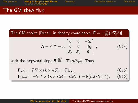
The GM choice [Recall, in density coordinates, F = − ∂∂ρ(κ∇ρh)]
A = Amn = κ
0 0 −Sx0 0 −SySx Sy 0
, (G14)
with the isopycnal slope Sdef= −∇hρ/∂zρ. Thus
Fadv = T∇× (k× κS) = TU? , (G15)
Fskew = −∇T × (k× κS) = κS∂zT − k(κS · ∇hT ) . (G16)
PO theory seminar, SIO, fall 2016 The Gent-McWilliams parameterization
The problem Mixing in isopycnal coordinates Summary Discussion questions References
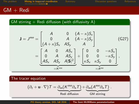
GM + Redi
GM stirring + Redi diffusion (with diffusivity A)
J = Jmn =
A 0 (A− κ)Sx0 A (A− κ)Sy
(A + κ)Sx ASy A
(G27)
=
A 0 ASx0 A ASy
ASx ASy A|S|2
︸ ︷︷ ︸
=Kmn
+
0 0 −κSx0 0 −κSyκSx κSy 0
︸ ︷︷ ︸
=Amn
,
The tracer equation
(∂t + u · ∇)T = ∂m(Kmn∂nT )︸ ︷︷ ︸Redi diffusion
+ ∂m(Amn∂nT )︸ ︷︷ ︸GM stirring
.
PO theory seminar, SIO, fall 2016 The Gent-McWilliams parameterization
The problem Mixing in isopycnal coordinates Summary Discussion questions References
Take home (or dump)
Summary
Quasi-adiabatic parameterization.
Tracer stirring performed by total (mean + eddy) velocity.
Tracer mixing can be equivalently represented by advective orskew fluxes.
(GM90: unclear, if not inconsistent, paper.)
Long live GM
There once was an ocean model called MOM,That occasionally used to bomb,
But eddy advection, and much less convection,Turned it into a stable NCOM.
(Limerick by Peter Gent)
PO theory seminar, SIO, fall 2016 The Gent-McWilliams parameterization
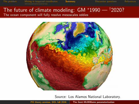
The problem Mixing in isopycnal coordinates Summary Discussion questions References
The future of climate modeling: GM ?1990 — †2020?The ocean component will fully resolve mesoscales eddies
Source: Los Alamos National Laboratory.
PO theory seminar, SIO, fall 2016 The Gent-McWilliams parameterization
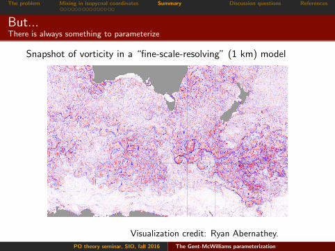
The problem Mixing in isopycnal coordinates Summary Discussion questions References
But...There is always something to parameterize
Snapshot of vorticity in a “fine-scale-resolving” (1 km) model
Visualization credit: Ryan Abernathey.
PO theory seminar, SIO, fall 2016 The Gent-McWilliams parameterization
The problem Mixing in isopycnal coordinates Summary Discussion questions References
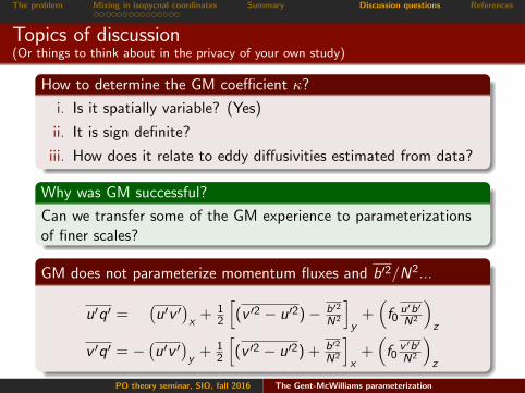
Topics of discussion(Or things to think about in the privacy of your own study)
How to determine the GM coefficient κ?
i. Is it spatially variable? (Yes)
ii. It is sign definite?
iii. How does it relate to eddy diffusivities estimated from data?
Why was GM successful?
Can we transfer some of the GM experience to parameterizationsof finer scales?
GM does not parameterize momentum fluxes and b′2/N2...
u′q′ =(u′v ′
)x
+ 12
[(v ′2 − u′2)− b′2
N2
]y
+(f0
u′b′
N2
)z
v ′q′ = −(u′v ′
)y
+ 12
[(v ′2 − u′2) + b′2
N2
]x
+(f0
v ′b′
N2
)z
PO theory seminar, SIO, fall 2016 The Gent-McWilliams parameterization
The problem Mixing in isopycnal coordinates Summary Discussion questions References
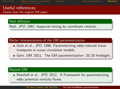
Useful referencesClearer than the original GM paper
Redi diffusion
Redi, JPO, 1982, Isopycnal mixing by coordinate rotation.
Better interpretations of the GM parameterization
Gent et al., JPO, 1996, Parameterizing eddy-induced tracertransports in ocean circulation models.
Gent, OM, 2011, The GM parameterization: 20/20 hindsight.
Beyond GM
Marshall et al., JPO, 2012, A Framework for parameterizingeddy potential vorticity fluxes.
PO theory seminar, SIO, fall 2016 The Gent-McWilliams parameterization