Genome-Wide Analysis of A-to-I RNA Editing in Drosophila · 2013-11-06 · Genome-Wide Analysis of A-to-I RNA Editing in Drosophila. Georges St. Laurent, Michael R. Tackett, Sergey

Genome-Wide Analysis of A-to-I RNA Editing in Drosophila

Georges St. Laurent, Michael R. Tackett, Sergey Nechkin, Dmitry Shtokalo, Denis Antonets, Yiannis A. Savva, Rachel Maloney, Philipp Kapranov, Charles E. Lawrence, and Robert A.

Reenan

Supplementary Figures 1-5

1. Supplementary Fig. 1: Discovery of Drosophila editing sites. 2. Supplementary Fig. 2: ECS editing and conservation of exonic sites. 3. Supplementary Fig. 3: Editing in non-coding RNAs. 4. Supplementary Fig. 4: Editing and alternative splicing. 5. Supplementary Fig. 5: Performance of different machine learning methods and

distribution of editing levels in the TP sites. List of Supplementary Tables Supplementary Notes 1-6

Nature Structural & Molecular Biology: doi:10.1038/nsmb.2675

0

500

1000

1500

2000

2500

3000

1 11 21 31 41 51 61 71 81 91 101 111 121 131 141 151 161

Num

ber o

f alig

ned

read

s

Editing Site

B

Supplementary Figure 1

A

Machine LearningAlgorithms

Sanger Validation

Basic Filters

True Positives

False Positives

ParameterRefinement

ADAR+ADAR-

gDNATotal RNA -> Ribodepletion -> cDNA

Helicos SMS

aligned readsunaligned reads

Align to Genomic SequenceAlign to Genomic Sequence + Splice Junctionsaligned reads

aligned reads

Sequence Read Database of A->G Substitutions

Call WT SNPsAlign in A=G & T=C space

Final Tier 1 List of ADAR Sites, Validation > 70%

False Positives‘Adjacent’ Sites

Lower Tier List of ADAR Sites, Validation < 70%

Master List of 3581 ADAR Sites, Accuracy 87%

0

1000

2000

3000

4000

5000

6000

0

0.2

0.4

0.6

0.8

1

(0.9

5-1]

(0.9

-0.9

5](0

.85-

0.9]

(0.8

-0.8

5](0

.75-

0.8]

(0.7

-0.7

5](0

.65-

0.7]

(0.6

-0.6

5](0

.55-

0.6]

(0.5

-0.5

5](0

.45-

0.5]

(0.4

-0.4

5](0

.35-

0.4]

(0.3

-0.3

5](0

.25-

0.3]

(0.2

-0.2

5](0

.15-

0.2]

(0.1

-0.1

5](0

.05-

0.1]

[0-0

.05]

RFss1 score

site

s

Expe

cted

TP/

(TP+

TN)

0

50

100

150

200

250

1 2 3 4 5 6 7 8 9 10

Num

ber o

f exo

nic s

ites

Bins of transcripts sorted by expression

0

500

1000

1500

2000

2500

0% 20% 40% 60% 80% 100%

Exons: ~345.1 M readsIntrons: ~31.4 M readsIntergenic: 130.4M reads

Num

ber o

f edi

ting

site

s

% of total number of reads

Estimated maximum of exonic sites ~1700

Number of exonicsites detected at ~31.4 M exonic reads

C

D E


Supplementary Figure 1. Discovery of Drosophila editing sites. (A) Distribution of SMS read coverage across known editing sites. The number of SMS reads (Y-axis) that map to each of 165 previously-known editing sites (X-axis; Supplementary Table 29) is plotted with the editing sites sorted by decreasing coverage. 60% of reads map to only 10% of the sites and the remaining 40% of reads cover the remaining 90% of sites. (B) The recursive discovery pipeline for the Drosophila. Total (rRNA-depleted) RNA from whole adult Wild Type flies served as the starting material for editing site discovery. To account for DNA polymorphisms and various other non-ADAR related artifacts, we also sequenced genomic DNA from Wild Type flies and total RNA (rRNA-depleted) from the ADAR null mutant. SMS reads were then imported into an alignment pipeline designed to select the highest quality alignments while completely avoiding penalties for A-to-G substitutions. Subsequent analysis resulted in a database of all possible sites. Basic Filters and application of Machine Learning Algorithms further filtered the database as described in the text. The key feature of the pipeline is a strong reliance on validation of randomly-selected sets of sites by Sanger sequencing to generate True Positives and True Negative sites, and further train our Random Forest-based models at each interaction. The results of the final version of the Random Forest-based model were partitioned with conservative thresholds to establish the Tier 1 list, and medium thresholds to populate the Tier 2 list, as described in the text. The final validation rates for the two Tiers were confirmed by Sanger sequencing of a random selection of sites. The Master List consists of all sites confirmed by Sanger and the Tier 1 list that validated at >70% for an estimated combined accuracy of 87%. (C) Separation of sites into three domains based on random forest model. Putative editing sites are distributed into 20 bins according to their RFss1 score (shown on the X-axis). The bins are split into Tier 1 (green), Tier 2 (yellow) and Tier 3 (red) sites based on the RFss1 score (see text for details). The vertical bars represent estimated TP ratios (TP/(TP+TN)) for each bin (left Y-axis). The black line indicates the number of putative sites in each bin (right Y-axis). (D) Editing site discovery and transcript levels. Annotated transcripts with exonic sites were distributed into 10 bins based on their expression level in Wild Type flies (X-axis), and the number of the exonic editing sites that fall into each bin is shown on the Y-axis. The bins are distributed from lowest (left) to highest (right). (E) Estimation of the total number of editing sites. Simulations were performed to determine the average number of editing sites that could be identified with decreasing subsets of our total informative reads (shown as percentage of total on the X-axis), and plotted here for exonic (blue), intronic (red) and intergenic (green) sites. Extrapolation of the asymptote for the exonic curve results in an estimation of ~1700 maximum exonic sites. Nature Structural & Molecular Biology: doi:10.1038/nsmb.2675

GCCA ACGAAAAG CGUCCGUCAAAU UGC UUUAGAUGAAC

CGGU UGCUUUAC GCGAGCAAUUUA ACG AAAUCUACUUG

5’

3’

UCA C

U AGA CUG AC UC

714 ntAA

C

AAA AGAAGACAGU UCAAAAAAUG ACCC

UUU UCUUCUGUCA AGUUUUUUAC UGGG

5’

GA A A C

C A AAG

AAAUAC GUA GCGAGAAUGUAU AUA AUCCUAU

UUUAUG CAU UGCUUUUACAUA UAU UAGGGUA

AA U U CU

CA U U A UAG

48 nt1,280 +/- 80 nt

308 +/- 35 nt3’

Site C

Site D

Site I

Site II

Site III

Site IV

||| |||||||||| |||||||||| |||| |||||| ||| ||| ||||||| ||| |||| ||

ScalechrX:

eageag

1 kb dm314,892,500 14,893,000 14,893,500 14,894,000

WT

FlyBase Protein-Coding Genes

12 Flies, Mosquito, Honeybee, Beetle Multiz Alignments & phastCons Scores

2 _

0 _

Site IV

Site III

Site II

Site I

Site ESite C

Site D

Wt Site C EgE1mt Site C EgE1 deletion Site C

B.

C.

|||| |||||| | || ||| |||| ||| |||||||||||

GCCA ACGAAAAG CGUCC UGC UUUAGAUGAAC

CGGU UGCUUUAC GCGAGCAAUUUA ACG AAAUCUACUUG

5’

3’

AAGCUUUUCA C

U AGA CUG AC UC

AA

CCGGU UGCUUUAC GCGAGCAAUUUA ACG AAAUCUACUUG

5’

3’

U AGA CUG AC UC

C

* *

After randomization

Editing Level

Con

serv

atio

n

Editing Level

Con

serv

atio

n


A.

D.


Supplementary Figure 2. ECS editing and conservation of exonic sites. (A) Examples of Intronic RNA editing sites residing within ECS elements. A. Four Intronic RNA editing sites (green) found within the known exonic complementary sequences that guide syt RNA editing in intronic (blue) and exonic (black) parts of the transcript. B. UCSC genome browser alignment of the eag genomic region spanning exon 12 to exon 13 (edited exon -red asterisk) contains highly conserved regions (green asterisk) across multiple Drosophila species. Hairpin drawing illustrates the predicted local structure surrounding eag editing sites C, D and E. The structure was generated using the Sfold web server. The highly conserved intronic element contains four editing sites (green). C. Schematics of the engineered mutations carried out by homologous recombination in the predicted ECS element to disrupt editing in the eag transcript. Specific mutation that alters the structural environment around site C and complete deletion of the intronic element abolishes RNA editing (Chromatograms). (D) Editing level vs sequence conservation of exonic editing sites. The sites were sorted based on editing level (X-axis). Conservation score (phastCons scores based on the 15-way alignment, Materials and Methods) was assigned for every site. Average conservation for i,i+1,…,i+199 sites was calculated in the sorted list, where i was from 1 to 1234. This smoothed conservation is shown on the Y-axis. Linear trend line was constructed to minimize sum of residual squares. Regression coefficient 0.2684 was significant with p-value<0.0001 based on 10000 permutations as shown on the right graph. The latter was generated with the same procedure but with the sites shuffled before averaging to randomize connection between the conservation and editing level. Nature Structural & Molecular Biology: doi:10.1038/nsmb.2675

5’

3’

GG

AA

G

UGU

A

U

UCU

GU

GA

UUG

UU

CU

G

UAC

AUUG

AU

CG

AU

A

UUC

AG

GU

AAC

U

GC A

UC

UG

CU U

AU

CA G

AU

CU

GU

UC

AG

AG

CCG

A

C

CC U

C

C

GU

CA

CA

C

CU U U

G

UG U

UU

CCC

A GU

AA

UU

C UG

C

CU

GG

CG

UU

GC

CG

UG

GC

U

C

CU C G

UU

C

GG

A

UC

GG

CUU

UC C

G

C

U

G

CC

U

U

CC

A

CU

GG

AU

GA

CG

A

C GG

GU

UA

UC

CG

GC

GG U

C G

A C

G

CAC

G

G

U

C

AU G

C

A

C

CCC

C G

AUC

C

G

U

C

G

C

C

C

C

CAC

C

AC

C

C

CG

C

G

G

AU

U

C

U

G

G

U

CU

C

GA

C

C

G

G

A

A

GC

C

G

UAU

UG

G

G

CG

G

G

GACG

G

G

C

G

G

C

G

G

U

C

CG

G

U

G

CU

GA

AG

C

C

G

G

C

GA

C

A

G

UUGC

C

C

G

A

G

UC

A

G

C

CA C

U

U

UCA A A A U U U G

U UG G U U A A G U A

A C U

UA

GUAGCUUAGCUU

CGGAUUUUC

GU

A

ACAA

A

U

U

U

GC

UG

UU

C

AG

AA

CACU

UC

CAUGU

ACG

CG

GC

A

UUG

CC

G

AGC

A

A

UUU

GC C C

A

U

U

CU

UUU

25

50

75

100

125

150

175

200

225

250

275

300

325

350375

400

425

37oΔG = -172.7

Edited

G

C

C

C

C

CAC

CIC

C

C

CG

C

G

G

AU

U

C

U

G

G

U

CU

C

GA

C

C

G

G

A

A

GC

C

G

UAU

UG

G

G

C

G

G

G

GACG

G

G

C

225

250

275

ΔG 37o = -167.3

Unedited

G

C

C

C

C

CAC

C

AC

C

C

CG

C

G

G

AU

U

C

U

G

G

U

CU

C

GA

C

C

G

G

A

A

GC

C

G

UAU

UG

G

G

CG

G

G

GACG

G

G

C

225

250

275


A

B

*

*

**

*

*

2R_T_5426564

3R_A_20225437

3L_A_13862666

3L_A_18793941

3R_T_2307512Scale

chr3R:

CG15186

1 kb dm32,306,000 2,307,000 2,308,000 2,309,000

WT


ESTs

5 _

0 _

Scalechr3L:

1 kb dm313,861,000 13,862,000 13,863,000 13,864,000

WT

FlyBase Protein-Coding GenesESTs

10 _

0 _

Scalechr3L:

ftz-f1CG14073

1 kb dm318,793,000 18,794,000 18,795,000 18,796,000

WT


ESTs

25 _

0 _

Scalechr2R:

brpbrpbrp

1 kb dm35,425,000 5,426,000 5,427,000 5,428,000

WT


ESTs

15 _

0 _

Scalechr3R:

nAcRalpha-96Aa

1 kb dm320,224,000 20,225,000 20,226,000 20,227,000

WT

FlyBase Protein-Coding GenesESTs

5 _

0 _


Supplementary Figure 3. Editing in non-coding RNAs. (A) Folding of edited and unedited forms of 7SK non-coding RNA. The folding was performed using the S-fold software (http://sfold.wadsworth.org). (B) Intergenic editing sites. Five representative intergenic sites are highlighted. On the left of each panel is the Sanger chromatogram of the wild type cDNA of the region, with the edited site indicated with an asterix. On the right, the genomic context of each site is provided, with the wild type SMS coverage (green), FlyBase genes (blue) and ESTs (black). The location of direction of transcription is indicated with a purple arrow and the edited site itself is indicated with a red triangle. Nature Structural & Molecular Biology: doi:10.1038/nsmb.2675

http://sfold.wadsworth.org/

1 2 3-4 5-6 7-9 >10010-100Number of isoforms

Index of editing

Index of gene length

0

50

100

150

200

250

300


Cumulative distribution of expressed spliced junctions/exons

Expressed spliced junctions/exons

A

B

00 1 2 3 4 5

K-S statistic = 0.38 Edited genes

Unedited genes

6

0.2

0.4

0.6

0.8

1.0

1.2


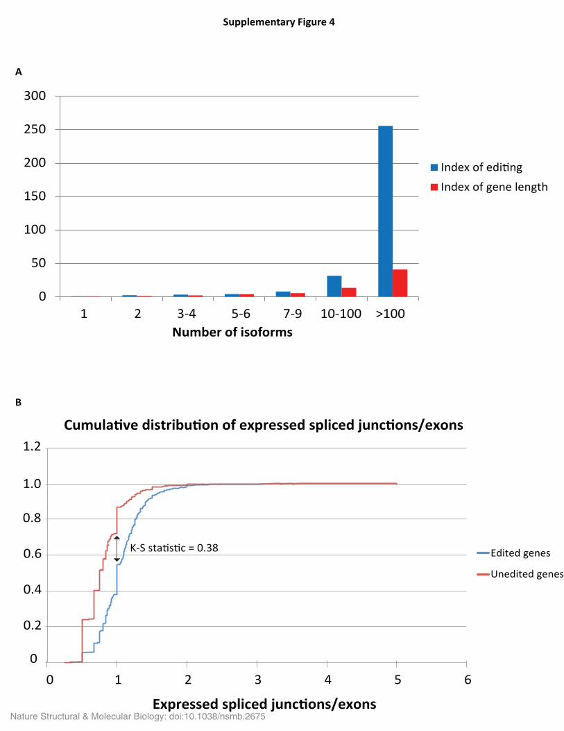
Supplementary Figure 4. Editing and alternative splicing. (A) Dependency of editing and gene length on the number of annotated isoforms. “Index of editing” (Y-axis) is the ratio of number of sites per gene in a given group vs number of sites per gene in the "1" group. “Index of length” (Y-axis) is ratio of average gene length in a given group and average gene length in the "1" group. (B) Distribution of splicing complexity of transcripts with and without editing sites. Cumulative distribution of expressed spliced junctions per annotated exons (X-axis) for edited (ble) and un-edited (red) genes is shown. Nature Structural & Molecular Biology: doi:10.1038/nsmb.2675

0%

2%

4%

6%

8%

10%

12%

1 51 101 151 201 251 301 351 401 451 501 551 601 651

Perc

ent e

dite

d

Editing site

Editing level

A

B



Supplementary Figure 5. Performance of different machine learning methods and distribution of editing levels in the TP sites. (A) Comparison of different machine learning approaches applied to detect real editing sites in Drosophila transcriptome. Different predictive classification models based on random forest algorithm (RF), sparse partial least squares (SPLS) and artificial neural networks (ANN) were constructed. Upper panel shows ROC curves (specificity vs sensitivity) produced for each of the models using different testing sets: 1). nearly balanced testing set, containing 78 TPs and 90 TNs, 2). the set of all validated sites excepting those used for training the models (533 TPs and 90 TNs) and 3). additional testing sets composed of poorly validated sites (31 TPs and 79 TNs). The lower panel shows PPV obtained with the models using the same three testing sets. PPV = TP/(TP+FP). Thus although ANN-based model demonstrated nearly the same AUC values as the RF-based one, ANN-based model had poor PPV, and thus RF algorithm was selected for further analysis. (B) Distribution of editing levels in the True Positive set of sites. The TP sites used to train the RF-based model were ranked (X-axis) by the editing level (Y-axis) as measured by the SMS RNAseq and the 681 sites with an editing level of 12% or less are shown. The curve represents the actual data and the line represents a regression fit. A breakdown in detection is not observed until the editing level reaches ~2%. Nature Structural & Molecular Biology: doi:10.1038/nsmb.2675

List of Supplementary Tables:

Supplementary Table 1 Overview of DNA and RNAseq datasets

Supplementary Table 2 Description of the variables used in RFA

Supplementary Table 3 Sanger Validations Performed

Supplementary Table 4 Master List of Drosophila Tier 1 Editing Sites

Supplementary Table 5 List of potential ECS sites

Supplementary Table 6 Measurement of editing levels of known sites in Wild Type and ADAR null

Supplementary Table 7 Classification of modENCODE sites into subsets

Supplementary Table 8 Conservation of genomically-encoded aminoacids changed by non-synonymous editing

Supplementary Table 9 DAVID Results, Swissprot Results, Flybase Results showing enrichment for editing in loci with alternative splicing potential

Supplementary Table 10 Link between splicing potential and editing

Supplementary Table 11 The 13 million site pipeline

Supplementary Table 12 List of Drosophila Tier 2 Editing Sites

Supplementary Table 13 The training samples used to build Random Forest algorithm-based model RFss1, as well as for training SPLS- and ANN-based models

Supplementary Table 14 The balanced testing data set used to validate RFss1, as well as SPLS- and ANN-based models

Supplementary Table 15 All but training samples used to validate RFss1, as well as SPLS- and ANN-based models (all the sites validated at the moment that were not used for training either model)

Supplementary Table 16 Poorly validated dataset used to validate RFss1, as well as SPLS- and ANN-based models (the sites that were predicted to be edited with our first SPLSDA-based model and that were not used for training either model)

Supplementary Table 17 Predictors used by RFss1 and description of spatial sign transformation (SST) procedure with R code examples

Supplementary Table 18 The training samples used to build RFss1 model after SST

Supplementary Table 19 The balanced testing data set for RFss1 validation (ST13) after SST


Supplementary Table 20 All but training samples for RFss1 validation (ST14) after spatial sign transformation (SST)

Supplementary Table 21 Poorly validated dataset for RFss1 (ST15) after spatial sign transformation (SST)

Supplementary Table 22 RFss1 model summary ant the R code used to build the model

Supplementary Table 23 The training samples used to build Random Forest algorithm-based model RF2

Supplementary Table 24 The balanced testing data set for RF2 model validation

Supplementary Table 25 All but training samples - all the sites validated at the moment that were not used for training RF2 model

Supplementary Table 26 Poorly validated dataset - the sites that were predicted to be edited with our first SPLSDA-based model and that were not used for training RF2

Supplementary Table 27 Four additional predictors used by RF2 and R code examples

Supplementary Table 28 RF2 model summary ant the R code used to build the model

Supplementary Table 29 List of previously known editing sites in Drosophila


SUPPLEMENTARY NOTE 1

RNA Preparation. Total RNA from whole male Canton-S (Wild Type) and dAdar null flies was isolated using TRIzol® reagent (Invitrogen) following the manufacturer’s protocol. Total RNA was then treated with DNase I as follows: 20µg of total RNA was mixed with 10µl TurboDNase Buffer (Applied Biosystems); 1µl RNaseOut (Invitrogen); and 2µl TurboDNase (Applied Biosystems) and incubated for 30 minutes at 37°C. The RNA was then purified using the RNeasy MinElute kit (Qiagen). The DNase I-treated RNA was fractionated using one of the following methods: (1) polyA+ fraction was isolated (2) depleted of ribosomal RNA (rRNA) using the RiboMinus Eukaryote kit (Invitrogen) (3) depleted of rRNA using an enhanced RiboMinus Eukaryote kit (Invitrogen and see below) (4) normalization. Ribosomal RNA Depletion. Samples underwent depletion of rRNA through the use of the RiboMinus Eukaryote Kit for RNA-Seq (Invitrogen, A10837-08) following the manufacturer's protocol. Samples that underwent enhanced ribosomal depletion had the manufacturer's protocol modified in the following ways: Oligos complimentary to the drosophila 18S and 28S rRNA transcript were purchased such that they each had a 5'-biotinylation (IDT) (see below for the list of oligos). The oligos were resuspended at 1000µM and an equimolar mastermix made. A total of 2000pmol oligo was added to 19µl DEPC water and the mixture incubated at 95°C for 5 minutes then rapidly cooled on ice. Eight microliters of 10mM ddNTP mixture (Roche), 4µl 2.5mM CoCl, 10x TdT buffer and 3µl Terminal Transferase (NEB) were added to the oligos and incubated at 37°C for 1 hour and 70°C for 10 minutes. The oligos were then cleaned twice on Performa DTR cartridges (EdgeBio) following manufacturer's protocols. The RiboMinus protocol was followed, except that 2.5µl of the prepared oligo mixture was added to the RNA prior to hybridization, when the RiboMinus probe was added. Synthesis of cDNA. Between 100-200ng of RNA was used for each cDNA synthesis reaction using the Superscript III kit (Invitrogen). Each sample of RNA was resuspended in 17µl DEPC water and incubated at 95°C for 5 minutes then rapidly cooled on ice. First, 10µl of 50ng/µl random hexamers and 2µl 10mM dNTP mix were added. The mixture was incubated at 65°C for 5 minutes then rapidly cooled on ice. Next, 5µl 10x buffer, 1µl 0.1M DTT and 10µl 25mM MgCl2 were added and the mixture incubated at 15°C for 20 minutes. Then 2.5µl RNaseOut and 2.5µl Superscript III were added and the samples incubated at 25°C for 10 minutes, 40°C for 40 minutes, 55°C for 50 minutes and 85°C for 5 minutes. Upon completion of cDNA synthesis RNA was removed by the addition of 1µl RnaseH and 1µl RNAseIf (NEB) and incubation at 37°C for 30 minutes. The resulting cDNA was then purified by the serial use of two Performa Gel Filtration Columns (EdgeBio) and quantified. PolyA tailing and 3' blocking. Using 100ng of the prepared cDNA in 28µl water, 5µl Helicos PolyA Control Oligo was added and the mixture incubated at 95°C for 5 minutes followed by rapid cooling on ice. A mixture of 5µl 2.5mM CoCl2, 5µl 10X Terminal deoxynucleotide Transfer (TdT) buffer, 5µl Helicos PolyA tailing dATP and 5µl TdT was then added to the sample and incubated at 42°C for 1 hour and


70°C for 10 minutes. The sample was denatured at 95°C for 5 minutes then rapidly cooled on ice. We then added 0.4µl biotinylated ddATP (Perkin Elmer) and 2µl TdT (NEB) and incubated the sample at 37°C for 1 hour and 70°C for 10 minutes to block the 3' tail of the cDNA. The sample was then digested with 1ul USER enzyme (NEB) and incubated at 37°C for 30 minutes to remove the control oligo. The sample was then purified using AMPure beads (Beckman Coulter) by bringing the volume up to 60µl and mixing with 72µl AMPure beads and incubating the mixture at room temperature for 30 minutes with intermittent agitation. Using a magnetic stand the beads were then collected and washed twice with 500µl 70% ethanol. The beads were allowed to dry for 5-10 minutes, resuspended in 20ul TE buffer and left on the stand for 5 minutes before the supernatant was removed. An additional 20ul elution was performed and pooled with the first. Normalization. Up to 1600ng of rRNA-depleted RNA (in eight 200ng aliquots) underwent cDNA synthesis as described above, with the exception that the 85°C incubation was replaced with a 10 minute incubation at 70°C followed by rapid cooling on ice. Second strand synthesis was performed by pooling the cDNA synthesis products and adding 1714µl DEPC water, 571µl 5x second strand buffer (Invitrogen), 57µl 10mM dNTPs (Invitrogen), 19.2µl 10U/µl E. coli DNA ligase (Invitrogen), 76µl 10U/µl E. coli DNA polymerase I (Invitrogen) and 19.2µl 2U/µl E. coli RNAseH (Invitrogen). The resultant mixture was distributed to pcr tubes and incubated at 16°C for 2 hours and 70°C for 15 minutes. The ds-cDNA was then purified on QIAQuick PCR cleanup kits (Qiagen) and eluted twice in 20µl TE. A target concentration of 100-150ng/µl is desired. Normalization occurs through the denaturation and re-hybridization of the ds cDNA followed by the selective degradation of ds-cDNA by Duplex-specific nuclease (DSN) (Evrogen). Three microliters of 100-150ng/µl ds cDNA were added to 1µl 4x hybridization buffer (200mM HEPES, pH 7.5, 2M NaCl), mixed thoroughly in a PCR tube and overlaid with 10ul Chill-Out liquid wax (Bio-Rad). Each sample was incubated at 98°C for 2 minutes and 68°C for 5 hours. Five microliters of preheated (68°C) 2x DSN Master Buffer (Evrogen) were added to each tube and the mixture incubated at 68°C for 10 minutes. One microliter of DSN enzyme (diluted to between 1U/µl and 1/16U/µl in 1x storage buffer) was added to each sample and incubated at 68°C for 25 minutes. Next 10ul DSN stop solution (Evrogen) was added to each tube followed by a 5 minute 68°C incubation. Finally 40µl water was added and the sample moved to ice to separate from the wax. The resulting normalized ds cDNA was then cleaned twice on Ampure beads as previously described and eluted in a final volume of 33µl TE.

A modified poly-A tailing and 3' end blocking was then performed on the samples. First 10.8ul of the normalized ds-cDNA (2-9ng total) was added to 2µl 2.5mM CoCl2 and 2µl 10x TdT buffer and the mixture denatured at 95°C for 5 minutes followed by rapid cooling on ice. One microliter TdT (diluted 1:4, NEB), 4µl 50µM dATP (Roche) and 0.2µl 10mg/ml BSA (NEB) were added and then the samples incubated at 37°C for 1 hour and 70°C for 10 minutes. The samples were then denatured at 95°C for 5 minutes followed by rapid cooling on ice. We then added 1µl 10x TdT Buffer, 1µl 2.5mM CoCl2, 0.5µl biotinylated ddATP (Perkin Elmer), 1µl (1:4 diluted ) TdT (NEB) and 6.5µl water and incubated the sample at 37°C for 1 hour and 70°C for 20 minutes. Two picomoles of Carrier Oligo (5'- TCACTATTGTTGAGAACGTTGGCCTATAGTGAGTCGTATTACGCGCGGT[ddC]-3' were added to the finished reaction.


Depletion Oligos: DM18S_1 /5Biosg/AGGAACCATAACTGATATAATGAGCCTTT DM18S_2 /5Biosg/GGTAGCCGTTTCTCAGGCTCCCTCT DM18S_3 /5Biosg/AGCTGGAATTACCGCGGCTGCT DM18S_4 /5Biosg/CGGTCCAAGAATTTCACCTCTCGCG DM18S_5 /5Biosg/GTTTCAGCTTTGCAACCATACTTCC DM18S_6 /5Biosg/ACTAAGAACGGCCATGCACCACCAC DM18S_7 /5Biosg/AGCCCAGGACATCTAAGGGCATCAC DM18S_8 /5Biosg/GGTAGTAGCGACGGGCGGTGTGTA DM18S_9 /5Biosg/GCATGGCTTAATCTTTGAGACAAGCA DM18S_10 /5Biosg/CCGGCCCACAATAACACTCGTTTAAGA DM18S_11 /5Biosg/TGGTTTCCCGGAAGCGACTGAGAGA DM28S_1 /5Biosg/TCCATTTTTAACGAACCAACGAAGAA DM28S_2 /5Biosg/TGACGCTCCATACACTGCATCTCA DM28S_3 /5Biosg/TTTCAACTTTCCCTCACGGTACTTG DM28S_4 /5Biosg/CATTTATTCTGTGTTAAAATGCAAGCAA DM28S_5 /5Biosg/TGTTTCAAGACGGGTCCCGAAGGTA DM28S_6 /5Biosg/GTTCACCATCTTTCGGGTCACAGCA DM28S_7 /5Biosg/TCGTTTCGACCCTAAGGCCTCTAATCA DM28S_8 /5Biosg/TTCCATGATCACCGTCCTGCTGTTT DM28S_9 /5Biosg/CATGCAGGCTTACGCCAAACACTTC DM28S_10 /5Biosg/TTGGAACCGTATTCCCTTTCGTTCA DM28S_11 /5Biosg/TGTCATGCTCTTCTAGCCCATCTACCA DM28S_12 /5Biosg/TCCCAATCAAGCCCGACTATCTCAA DM28S_13 /5Biosg/GATTCCCCAAGTCCGTGCCAGTTCT DM28S_14 /5Biosg/TCGTTAATCCATTCATGCGCGTCAC DM28S_15 /5Biosg/TCATTGACGATACCAAACCGAGGTC DM28S_16 /5Biosg/CCTGGCAATGTCCTTGAATTGGATCA DM28S_17 /5Biosg/TGAGAGATGTACCGCCCCAGTCAAA DM28S_18 /5Biosg/CCGCCACAAGCCAGTTATCCCTATG DM28S_19 /5Biosg/TCAGGCATAATCCAACGGACGTAGC DM28S_20 /5Biosg/TATGTAACTAGCGCGGCATCAGGTG DM28S_21 /5Biosg/TCAGGGGGTAGTCCCATATGAGTTGAGG DM28S_22 /5Biosg/TGCTCAAGGTACGTTCCAGTTAGAGG DM28S_23 /5Biosg/TCGTTCCTGTTGCCAGGATGAGCAC DM28S_24 /5Biosg/CCTTGGAGACCAGCTGCGGATATTGGT DM28S_25 /5Biosg/CCGGGGAACAAGTAACTAACATAAATGC Standard Sequence Alignments

Raw Helicos SMS reads from Wild Type and ADAR- mutant flies were trimmed for leading stretches of T residues and filtered for machine artifacts as described earlier1,2. The minimal length of post-trimming reads was set to 25 bases. Overall, after filtration 3.9B Wild Type reads corresponding to 173 channels and 2.0B ADAR- reads corresponding to 117 channels were obtained. Those were then aligned to DM3 reference genome supplemented with all known


splice junctions based on FlyBase annotations and a number of fly rDNA sequence from GenBank. In addition, for each locus we created a set of all theoretically-possible splice junctions and add them to the reference sequences. Alignments were performed with the indexDPgenomic aligner3 with a minimum normalized score of 4.31,2. Overall, 1.5B WT reads and 0.74B ADAR- RNAseq reads were successfully aligned to the reference allowing for reads mapping in multiple location with the same score. We also generated 243M aligned DNAseq reads from Wild Type flies corresponding to the average coverage of the fly genome of 42x. Important, due to the limitation of the aligner, reads whose seeds mapped in more than 25 locations were omitted, thus very few of the reads mapping to rDNAs represented by multiple copies in our reference were captured. RNAseq reads not aligned in the first pass alignment with standard score matrix that would penalize A-to-G substitutions were then re-aligned in a different regime where score for A-to-G or T-to-C substitutions (reference->read) was set to be the same as for the matching bases. The latter was used to account for the bottom strand transcripts. These alignments were combined with the standard alignments for the downstream processing.For each RNAseq read, we captured all possible alignments above the score of 4.3, not just the alignments with the best score. This was done to allow for subsequent removal of reads whose mapped positions were relatively close in sequence to positions elsewhere in the genome. We further filtered all alignments with a minimum normalized score of 4.5 and then removed all reads that had a second best alignment with a score of 4.5 or above and reads that had more than 1 alignment anywhere in the reference with the same score and any reads mapping to rDNA or chrM. After this filtration step, 413.8M Wild Type reads and 95.6M ADAR- reads remained. The former yielded 13M of A-to-G sites on either strand of the reference sequence almost entirely representing sequence errors.

Editing site discovery: Machine Learning Classification.

For building classifiers we tried sparse partial least squares (SPLS) algorithm implemented in R package spls4, artificial neural network (ANN) package neuralnet (http://CRAN.R-project.org/package=neuralnet) and random forest algorithm5 implemented in R package randomForest6. All machine learning models were trained on true positive (TP) and true negative (TN) sites derived from the Sanger validation.

The TN sites corresponded to sites that passed some of our basic filters and thus represented areas of genome potentially susceptible to technological errors, such as areas prone to misalignments and other issues. The quality of produced models was assessed using the following criteria: specificity (TN/N), sensitivity (TP/P), AUC – the area under receiver operating characteristic curve, and positive predictive value (TP/(TP+FP)). Performance of generated models was assessed with ROCR package7,8. All predictive models were built using R environment for statistical computing9. For training and tuning the models and for partitioning the data we used caret (Classification And REgression Training) package for R10.

To produce the first generation of our SPLS, ANN and RFA-based models we used the set of sites with A-to-G substitutions validated with Sanger sequencing – the set containing 877 sites (660 TPs and 217 TNs). Original data was prepared for further analysis: raw numbers of reads with certain nucleotides were recalculated as ratios – to make it possible to compare one site with another. Besides, some parameters, like raw numbers of G-containing reads and the number of total reads were also used, since they could reflect the quality of our sites. Indeed, if two sites


demonstrating 20 % of G-containing reads and 80 % of A-containing have drastically different numbers of total reads, e.g. 12 and 120, the last one is less likely to be erroneous.

At first we tried to build the models using unbalanced training sets since our Sanger validations contained more TPs, however the resulting models were later found to be inaccurate. We also tried to use different weights for TP and TN classes, but the resulting models were found to produce significantly more false positives. Then we became to use only balanced training sets, containing equal numbers of TPs and TNs, that were produced by down sampling the set of our TP sites. All the data, used to train and test the models, as well as description of used predictor variables could be found within the Supplementary Tables. The balanced training set used to build RFss1 (Random Forest–based classifier after Spatial Sign transformation), as well as for training SPLS- and ANN-based models is shown in Supplementary Table 13, the balanced testing set – in Supplementary Table 14, all but the training samples – in Supplementary Table 15.

Surprisingly, although with testing procedure the SPLS-based classifier was initially found to perform very well (with AUC > 0.94), subsequent validation have shown that its results were too optimistic, since using subsequent validation results as a testing set we obtained poor AUC value that was equal to 0.67. The set was found to contain only 31 TPs and 79 TNs (Supplementary Table 16) while SPLS-based model predicted all of them to be edited. This might be due to some non-linear and non-monotonic relations between our predictive variables. Thus we built predictive models based on artificial neural networks and random forest algorithm. Comparison of our best ANN- and RFA-based classifiers together with SPLS-based one have shown that RFA-based model performed the best, since although all the models demonstrated similar AUC values using different testing sets, RFA-based model was found to have the best PPV (positive predictive value) among the others for all used testing sets. RFA was found to be the best using the “twilight zone” samples (those with low coverage, predicted to be edited with SPLS), that were incorrectly classified by other methods. Results of this comparison are shown on Supplementary Fig. 5a.

RFA is an ensemble learning technique producing many decision trees, and the resulting prediction corresponds to classification with the most votes. Each tree is constructed with bagging procedure – random bootstrap sampling of the data and out-of-bag examples – those not used for growing the tree – are used to estimate prediction error. For each node for every decision tree the best split is selected from the set of randomly chosen predictor variables. As compared to many other machine learning algorithms RFA turns out to be more robust towards both outliers and overfitting issues. Another advantage of RFA is that it able to estimate the Gini importance of individual predictors – the value describing the contribution of individual variable to overall classification, and thus this algorithm could be used for feature selection.

At first we produced a model that used 77 predictors (Supplementary Table 2). The data was preprocessed with spatial sign transformation (SST)11. SST was applied as a more robust alternative to the standard scaling procedure (centering around the mean and scaling by standard deviation), since both mean value and standard deviation are highly sensitive to outliers in the data. The SST procedure and corresponding R code are shown in Supplementary Table 17. This random forest model (RFss1) was produced using the balanced training set, containing 127 TPs and 127 TNs (Supplementary Table 18) with 10-fold cross-validation. It was tuned with caret R package10. Its performance was assessed using three different testing sets: nearly


balanced one containing 90 TNs and 78 TPs (Supplementary Table 19), heavily unbalanced set with 90 TNs and 533 TPs (Supplementary Table 20) and validated set with 79 TNs and 31 TPs (all these samples were predicted as positives with our SPLS model; Supplementary Table 21). All the training and testing sets contain the same sites as ST12-15 but these data underwent spatial sign transformation. The parameters of RFss1 models and the R code used to build it could be found in Supplementary Table 22. Final RFss1 model contained 500 trees, number of variables tried at each split was equal to 5, and estimated out-of-bag error was 15.35 %. On average 33.9 predictor variables were selected.

Our RFA-based RFss1 model was used to rank individual variables according their Gini importance (Fig. 3b, Supplementary Table 2). RFss1 selected optimal predictor variables and, according to Gini importance measures, the most informative criteria were those describing the average length of G-containing reads (for certain genomic position) in all alignments produced with either 4- (normal) or 3-letter alphabets from both strands for wild type flies (wt_t_AGRL - wild-type total average G-read length), the percent of G-containing reads in normal alignments of sense reads of wild type flies (wt_nsG - wild-type normal sense G-reads ratio), the ratio of 3-letter aligned A-reads to normal G-reads of wild-type flies (A3let_nG_rat), the ratio of 3-letter aligned A-reads to normal G-reads for adar -/- flies (adA3let_n_rat), ratio of A-reads percentage of wild-type flies to that of adar -/- flies (wt2adA), ratio of G-reads percentage of wild-type flies to that of adar -/- flies (wt2adG), percent of A-containing reads in normal alignments of sense reads of wild type flies (wt_nsA), total number of G-containing reads in wild-type flies (wt_tGreads), the ratio of 3-letter aligned G-reads number to the total number of G-reads of wild-type flies (G3let_tot_rat), average distance between A-to-G transition and the nearest end of the read in all kinds of alignments in wild-types(wt_t_AMED - average mismatch edge distance), and mean square deviation of that values (wt_t_MEDMSD - mismatch edge distance mean square deviation), and the ratio of 3-letter aligned A-reads number to the total number of A-reads in wild-types (A3let_tot_rat). All these parameters and more (Supplementary Tables 13-16, 18-21, and 23-26) were calculated for each site from all the candidates with A-to-G transitions.

After subsequent Sanger validation we produced the second random forest model RF2. It was built using the unscaled data, as after collecting more validated sites SST was found to have only minor impact on prediction quality. The resulting set of validated sites contained 1321 sites with 995 TPs and 326 TNs. RF2 was trained using balanced training set with 265 TPs and 265 TNs (Supplementary Table 23) and it was tested with three different testing sets: balanced one containing 113 TNs and 113 TPs (Supplementary Table 24), unbalanced one with 113 TNs and 982 TPs (Supplementary Table 25) and validation set with 79 TNs and 31 TPs (Supplementary Table 26). Besides descriptors used by RFss1, RF2 used four additional variables: A-richness (A% in -20/+20 bp regions around the putative editing sites), two different sequence context scores based on nucleotide triplets (-1/+1 regions) analysis and linguistic complexity. Linguistic complexity was calculated for the -20/+20 regions using TraMineR package14. Description of these parameters and the R code with TraMineR usage example are shown in Supplementary Table 27. RF2 was built using 3 times repeated 5-fold cross-validation and tuned with caret package. On average 38.74 predictor variables were selected. RF2 contained 500 trees; number of variables tried at each split was 20; RF2 estimated out-of-bag error was 11.32 %. The R code used to build the model and RF2 parameters could be found in Supplementary Table 28.


Each model was later assessed with Sanger validations of randomly-selected sites. 3D projection of the samples was created with robust principal component analysis (PCA) using pcaPP R package12.

Application of our advanced filtering procedure yielded three tiers of predicted sites. (Tier 1, Tier 2, and Tier 3; Supplementary Fig. 1c). The “TP ratio” (TPs/(TPs+TNs)), from our advanced filtering procedure predicts the proportion of valid sites in each pool. Tier 3 had 26.5K candidate sites (RFA score <= 0.30) and a predicted TP ratio of less than 5%, thereby eliminating it from further analysis. Tier 2 had 13.5K candidate sites (0.575 >= RFA Score > 0.30), with expected TP ratio of 24% , and Tier 1 had 2.5K candidate sites (RFA Score >= 0.575) with expected TP ratio of 80%. Sanger sequencing of a set of 205 randomly selected candidate sites from Tier 1 resulted in a validation rate of 73.6% (95% confidence interval is 69.2% to 78%), in rough agreement with the expected TP ratio of 80% for this domain. The high validation rate in Tier 1, together with sites discovered in previous steps of the pipeline, resulted in a total of 3,581 high confidence editing sites (the Master List), including 2,590 high-quality novel sites found in this work (Supplementary Table 4, Fig. 3e). A similar set of 125 randomly selected candidate sites from Tier 2 resulted in a validation rate of 9.3% (95% confidence interval +/-2.9%), indicating that an additional 1,252 editing sites exists within the Tier 2 list (Supplementary Table 12). To calculate the confidence interval on the total number of sites in both tiers (4.8K), we used the following logic. Tier2 has 13,465 sites validated at 9.3%, with the 95% confidence interval giving the number of true sites in that Tier at 862 to 1,643 true sites. In addition, we have 3,581 high confidence sites in the Master list. After adding them, we get 4,443 to 5,224 sites are in the Master list and Tier2.


In addition, we observed an increase in conserved exonic sites at the very lowest editing levels: 200 sites with between 2.7% and 5.7% editing have 0.71 average phastCons score, and 125 (62.5%) of them had a conservation value of 0.9 or greater, possibly indicating tissue specific editing, or a set of evolutionarily conserved and “poised” editing sites available for editing under special biological or environmental circumstances.. Since our RNA sample was obtained from whole organism, the conserved lower level editing site could possibly represent editing in a cell- or tissue-specific manner, or a set of evolutionarily conserved and “poised” editing sites available for editing under special biological or environmental circumstances.


Only 37 additional Ramaswami et. al. sites were supported by Rodriguez et. al. sites (Fig. 3e). Also, of the 514 modENCODE sites, only an additional 24 were supported by Rodriguez et. al. (Fig. 3e).



Reciprocally, of the three conservation categories, the non-synonymous SNPs favored amino acids conserved in only the 1-4 species category: 42.2%, 53.3% and 30.6% of amino acid changes in the three categories were found in this least conserved category. The corresponding numbers for non-synonymous editing were 5.7%, 9.8% and 6.8% (Fig. 4, Supplementary Table 8).


As amino acid conservation is a indicator of important positions in the protein that have effects on functionality, bias towards conserved amino acids implies targeted recoding of such amino acid residues by RNA editing. In this context, 71 non-synonymous sites recoded amino acids conserved in at least 12 species to structurally very different amino acids and are likely to cause major perturbation in protein function.


The high level of read and alignment errors in high throughput technologies also makes validation important for most other studies based on large sequencing datasets. Unfortunately, the high level validation employed in this study is often not feasible in other genome studies. However, as we illustrated with our own prediction and the modENCODE predictions, the validation of a modest number of randomly sampled predictions provides a means to estimate the proportion of a study’s predictions that are valid, and specify an interval that contains the true proportion valid with high confidence. In addition, we show in another manuscript that validation and reproducibility are not the same, because the former does not include variation stemming from biological and sample preparation variability. To assess reproducibility validations in multiple biological replicas are required (Alpert et.al, 2013, in press).

At the same time, the data we report here also has limitations. First, due to limits of detection of rarely expressed transcripts, we are unable to detect highly cell-type specific editing events. Second, the minimal level of editing reliably detected in our study is approximately 2% (Supplementary Fig. 5b). Also the fact that we extracted RNA from whole flies limits our findings in two ways. Firstly, since editing occurs in the nucleus, events in introns and intergenic regions almost certainly underrepresented in our results. Nevertheless, we were able to report a large number of novel edit sites in introns and intergenic regions. We excluded editing events occurring in sequences with identical or near identical copies present elsewhere in the genome; we can detect editing only in unique portions of repeat regions. Finally, we only examined male Drosophila grown under standard laboratory conditions, and we expect that environmental changes may result in at least a partial change in the repertoire of editing sites within the organism13.


1. Kapranov, P. et al. New class of gene-termini-associated human RNAs suggests a novel RNA copying mechanism. Nature 466, 642-6 (2010).

2. Lipson, D. et al. Quantification of the yeast transcriptome by single-molecule sequencing. Nat Biotechnol 27, 652-8 (2009).

3. Giladi, E. et al. Error tolerant indexing and alignment of short reads with covering template families. J Comput Biol 17, 1397-1411 (2010).

4. Chun, H. & Keles, S. Sparse partial least squares regression for simultaneous dimension reduction and variable selection. J R Stat Soc Series B Stat Methodol 72, 3-25 (2010).

5. Breiman, L. Random Forests. Machine Learning 45, 5-32 (2001). 6. Liaw, A & Weiner, M. Classification and regression by random forest. R News 2, 18-22 (2002). 7. Diaz-Uriarte, R. & Alvarez de Andres, S. Gene selection and classification of microarray data

using random forest. BMC Bioinformatics 7, 3 (2006). 8. Sing, T., Sander, O., Beerenwinkel, N. & Lengauer, T. ROCR: visualizing classifier performance

in R. Bioinformatics 21, 3940-1 (2005). 9. R Development Core Team. R: A language and environment for statistical computing. 409

(2009). 10. Kuhn, M. Building Predictive Models in R Using the caret Package. J Stat Softw 28, 1-26 (2008). 11. Serneels, S., De Nolf, E. & Van Espen, P.J. Spatial sign preprocessing: a simple way to impart

moderate robustness to multivariate estimators. J Chem Inf Model 46, 1402-9 (2006). 12. Croux C, F.P., Oliveira MR. Algorithms for Projection-Pursuit Robust Principal Component

Analysis. Chemometrics and Intelligent Laboratory Systems 87, 218-225 (2007). 13. Jepson, J.E. et al. Engineered alterations in RNA editing modulate complex behavior in

Drosophila: regulatory diversity of adenosine deaminase acting on RNA (ADAR) targets. J Biol Chem 286, 8325-37 (2011).


Documents

Genome-Wide Analysis of A-to-I RNA Editing in Drosophila · 2013-11-06 · Genome-Wide Analysis of A-to-I RNA Editing in Drosophila. Georges St. Laurent, Michael R. Tackett, Sergey