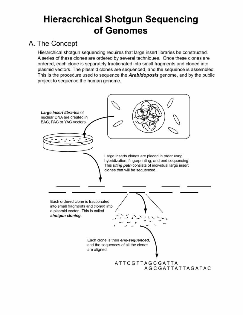
Genome Sequencing

Principals of a genome project for a species • Identify the reference line

o Typically the line has been used historically in genetic research

o Or, a resource is available for the line Clone library Mutant lines Mapping parent

• Isolate high quality DNA • Apply some sequencing approach that fits the budget • Collect DNA • Assembly the reads into

o Contigs o Scaffolds

• Order scaffolds using a genetic map into pseudochromosomes • Annotate the genes • Use the reference genome in research

o Discover candidate gene(s) that control a phenotype o Develop markers to tract important genes/regions of the

genome

Approach to the Actual Genome Sequencing • Fragment the genomic DNA • Clone those fragments into a cloning vector • Isolate many clones • Sequence each clone

Sequencing Techniques Were Well Established

• Sanger was used for the past twenty years • Helped characterize many different individual genes. • Previously, the most aggressive efforts

o Sequenced 40,000 bases around a gene of interest How is Genomic Sequencing Different???

• The scale of the effort o Example

Public draft of human genome • Hierarchical sequencing • Based on 23 billon bases of data

Private project (Celera Genomics) draft of human genome

• Whole genome shotgun sequencing approach • Based on 27.2 billon clones • 14.8 billion bases

Result: • Human Genome = 2.91 billion bases

Changes That Facilitated Genomic Sequencing • Sequencing

o Basic technique is still the same • Major changes

o Thermostable polymerase enzymes Improves quality of sequencing products

o Fluorescently labeled nucleotides for the reaction Allows for laser detection

o Laser-based detection systems 8, 16 or 96 samples analyzed simultaneously

o Results for a single run 500-700 bases of high quality DNA sequence data

o Human Project peak output 7 million samples per month 1000 bases per second

• Robotics o Key addition to genomic sequencing o Human hand rarely touches the clone that is being sequenced o Robots

Pick subclones Distribute clones into reaction plates Create the sequencing reaction Load the plates onto the capillary detection system

o Result Increased the quality and quantity of the data Decreasing the cost

• Dropped over 100 fold since 1990 Improvements felt in small research lab

o Sequence reads today $2.50 vs. $15 in the early 1990s.

Hierarchical Shotgun Sequencing • Two major sequencing approaches

o Hierarchical shotgun sequencing o Whole genome shotgun sequencing

• Hierarchical shotgun sequencing o Historically

First approach o Why???

Techniques for high-throughput sequencing not developed

Sophisticated sequence assembly software not availability

• Concept of the approach o Necessary to carefully develop physical map of overlapping

clones Clone-based contig (contiguous sequence)

o Assembly of final genomic sequence easier o Contig provides fixed sequence reference point

• But o Advent of sophisticated software permitted

Assembly of a large collection of unordered small, random sequence reads might be possible

o Lead to Whole Genome Shotgun approach

Steps Of Hierarchical Shotgun Sequencing

• Requires large insert library o Clone types

YAC (yeast artificial chromosomes) • Megabases of DNA • Few (several thousand) overlapping clones

necessary for contig assembly • But

o YACs are difficult to manipulate o Most research skilled with bacteria but not

yeast culture • Rarely, if ever, used today

BAC or P1 (bacterial artificial chromosomes) • Primary advantages

o Contained reasonable amounts of DNA about 75-150 kb (100,000 – 200,000)

bases o Do not undergo rearrangements (like YACs) o Could be handled using standard bacterial

procedures

Developing The Ordered Array of Clones

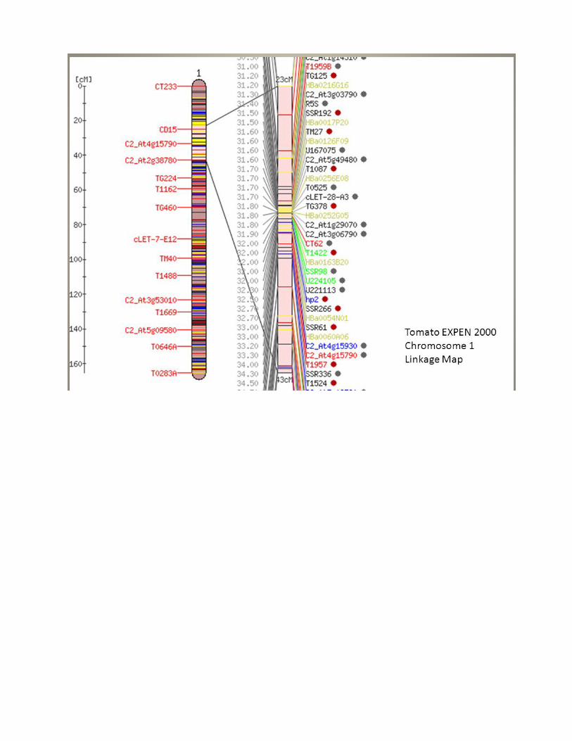
• Using a Molecular Map o DNA markers o Aligned in the correct order along a chromosome o Genetic terminology

Each chromosome is defined as a linkage group o Map:

Is reference point to begin ordering the clones Provides first look at sequence organization of the

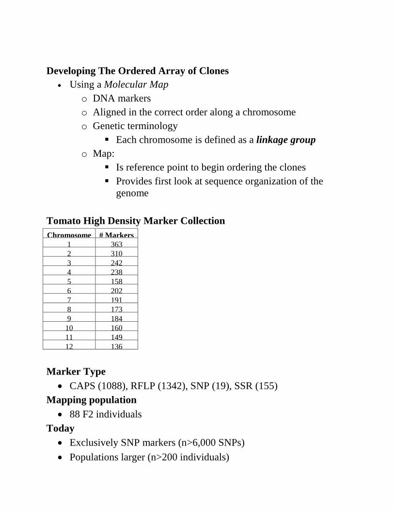
genome Tomato High Density Marker Collection Chromosome # Markers

1 363 2 310 3 242 4 238 5 158 6 202 7 191 8 173 9 184 10 160 11 149 12 136

Marker Type

• CAPS (1088), RFLP (1342), SNP (19), SSR (155) Mapping population

• 88 F2 individuals Today

• Exclusively SNP markers (n>6,000 SNPs) • Populations larger (n>200 individuals)

Developing a Minimal Tiling Path

• Definition o Fewest clones necessary to obtain complete sequence

• Caution is needed o Clones must be authentic o Cannot contain chimeric fragments

Fragments ligated together from different (non-contiguous) regions of the genome

o How to avoid chimeras and select the minimum path Careful fingerprinting

• Overlapping the clones

o Maps not dense enough to provide overlap o Fingerprinting clones

Cut each with a restriction enzyme (HindIII) Pattern is generally unique for each clone Overlapping clones defined by

• Partially share fingerprint fragments o Overlapping define the physical map of the genome

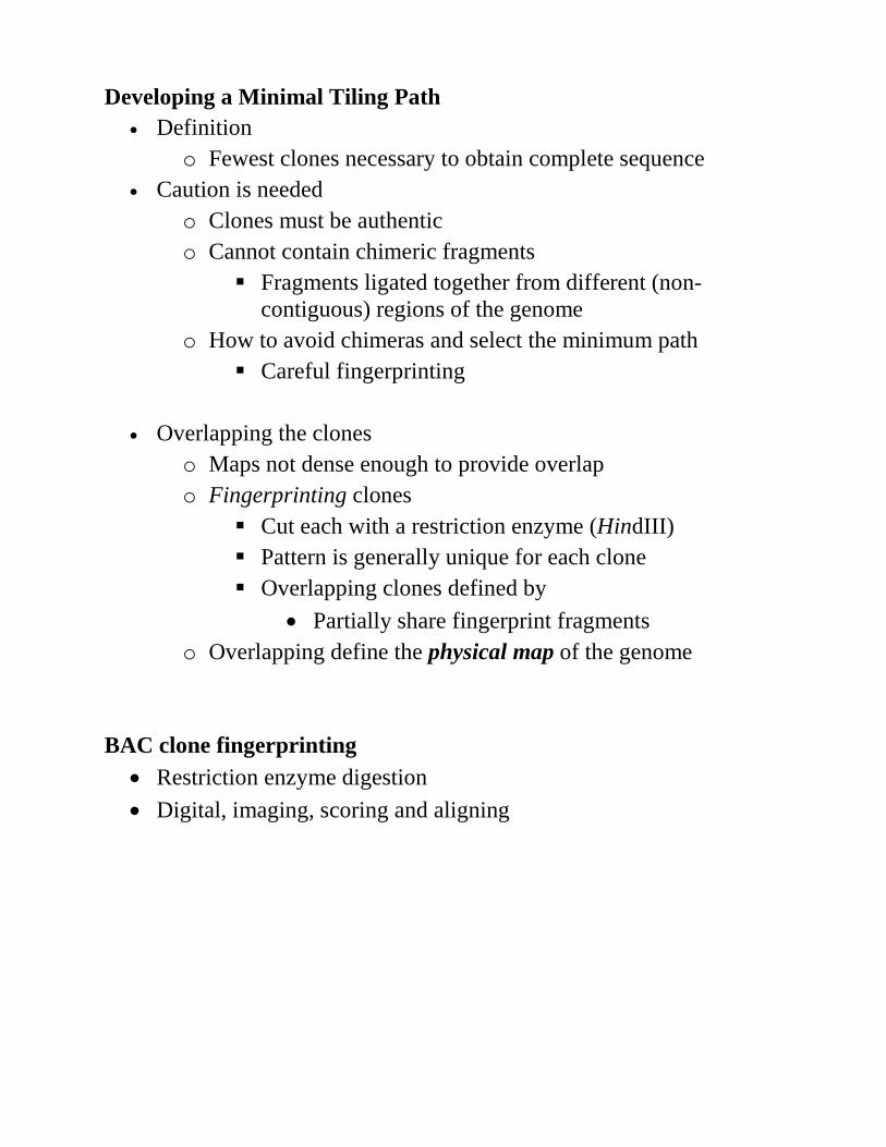
BAC clone fingerprinting

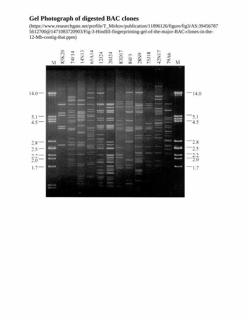
• Restriction enzyme digestion • Digital, imaging, scoring and aligning

Gel Photograph of digested BAC clones (https://www.researchgate.net/profile/T_Mirkov/publication/11896126/figure/fig3/AS:394567875612700@1471083720903/Fig-3-HindIII-fingerprinting-gel-of-the-major-BAC-clones-in-the-12-Mb-contig-that.ppm)

Digital Image of Clones (https://www.researchgate.net/figure/6535067_fig5_Fig-5-Example-of-the-clone-order-fingerprints-of-a-BAC-contig-of-the-apple-physical)

Genomic Physical Maps • Human

o 29,298 large insert clones sequenced More than necessary Why???

• Genomic sequencing began before physical map developed

• Physical map was suboptimal • Arabidopsis

o 1,569 large insert clones defined ten contigs Map completed before the onset of sequencing Smaller genome

• about 125 megabases • Yeast

o 493 cosmid (smaller insert clones) clones Relatively high number of clones for genome size

Other Uses Of A Physical Maps

• Rich source of new markers • Powerful tool to study genetic diversity among species • Prior to whole genome sequencing

o Markers can locate a target gene to a specific clone o Gene can be sequenced and studied in depth

Sequencing Clones Of The Minimal Tiling Path

• Steps o Physically fractionate clone in small pieces o Add restriction-site adaptors and clone DNA

Allows insertion into cloning vectors • Plasmids current choice

o Sequence data can be collected from both ends of insert Read pairs or mate pairs

• Sequence data from both ends of insert DNA • Simplifies assembly • Sequences are known to reside near each other

Assembly of Hierarchical Shotgun Sequence Data

• Process o Data collected o Analyzed using computer algorithms o Overlaps in data looked for

• Accuracy levels o Analyzing full shotgun sequence data for a BAC clone

Goal: 99.9% accuracy 100 kb BAC clone

• 2000 sequence reads • Equals 8-10x coverage of clone • Typical level of accuracy that is sought

Primary software used is Phrap • Phrap = f(ph)ragment assembly program • Efficient for a “small” number of clones

o Small relative to number from a whole genome shotgun approach

• Each sequence read is assesses for quality by the companion software Phred

• Assembles sequence contigs only from high quality reads

o Working draft sequence 93-95% accuracy 3-5 x coverage of 100 kb BAC clone

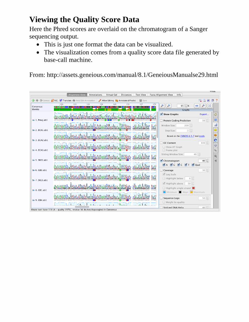
Viewing the Quality Score Data Here the Phred scores are overlaid on the chromatogram of a Sanger sequencing output.

• This is just one format the data can be visualized. • The visualization comes from a quality score data file generated by

base-call machine. From: http://assets.geneious.com/manual/8.1/GeneiousManualse29.html

Finishing The Sequence • Gaps need to be filled

o Study more clones Additional subclones sequenced Tedious and expensive

o Directed sequencing of clones or genomic DNA used Create primers near gaps

• Amplify BAC clone DNA o Sequence and analyze

• Amplify genomic DNA o Sequence and analyze

Confirming the Sequence

• Molecular map data o Molecular markers should be in proper location

• Fingerprint data o Fragment sizes should readily recognized in sequence data

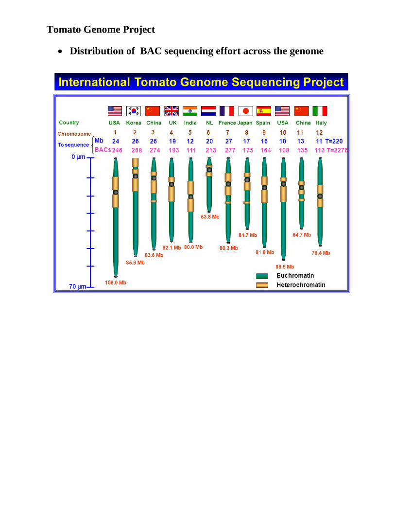
Tomato Genome Project

• Distribution of BAC sequencing effort across the genome

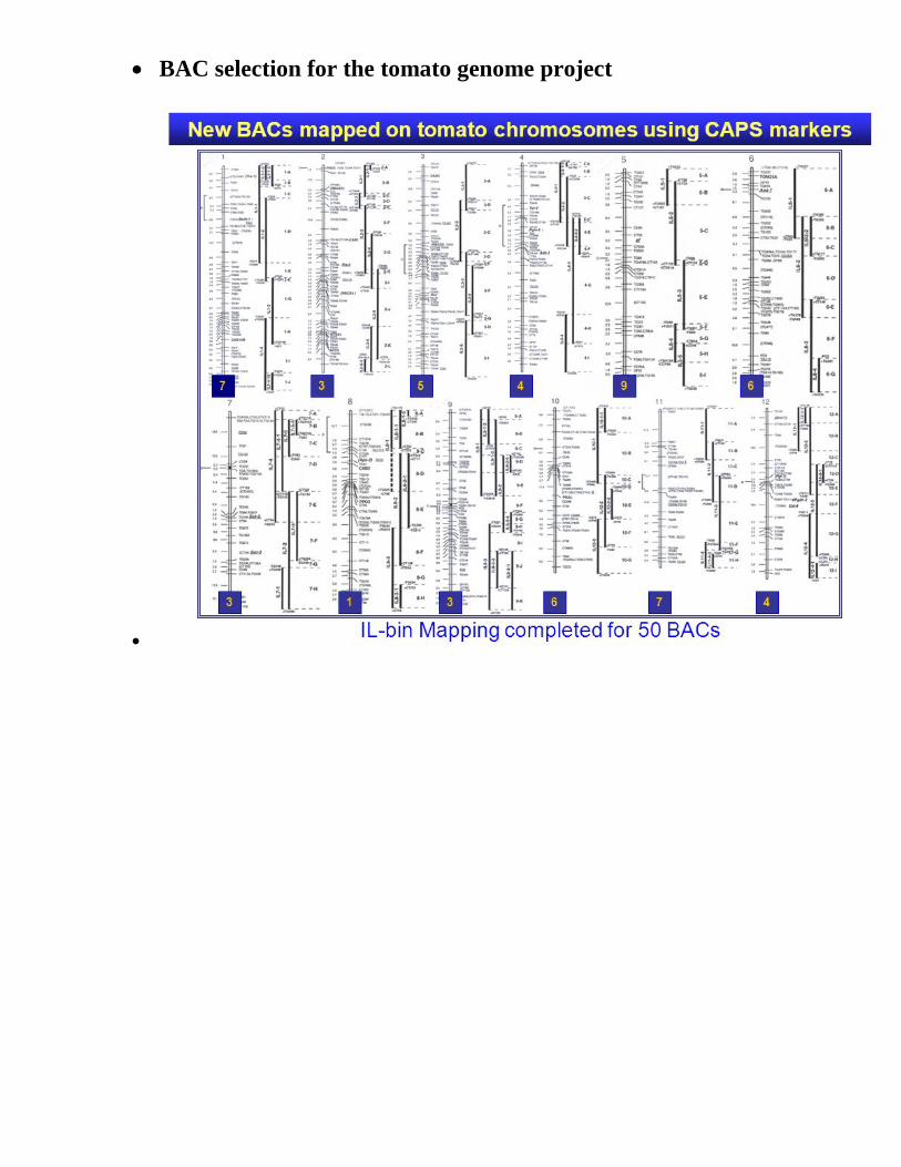
• BAC selection for the tomato genome project

•

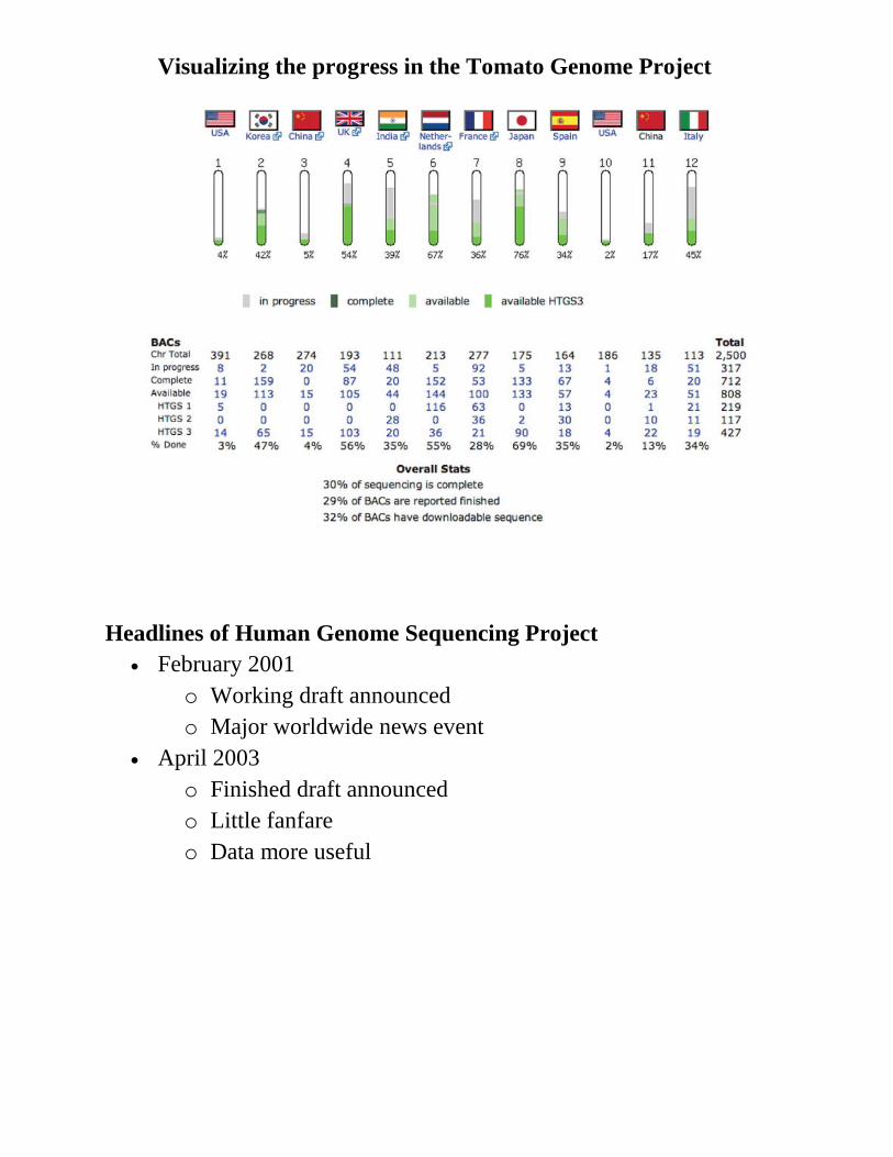
Visualizing the progress in the Tomato Genome Project

Headlines of Human Genome Sequencing Project

• February 2001 o Working draft announced o Major worldwide news event

• April 2003 o Finished draft announced o Little fanfare o Data more useful

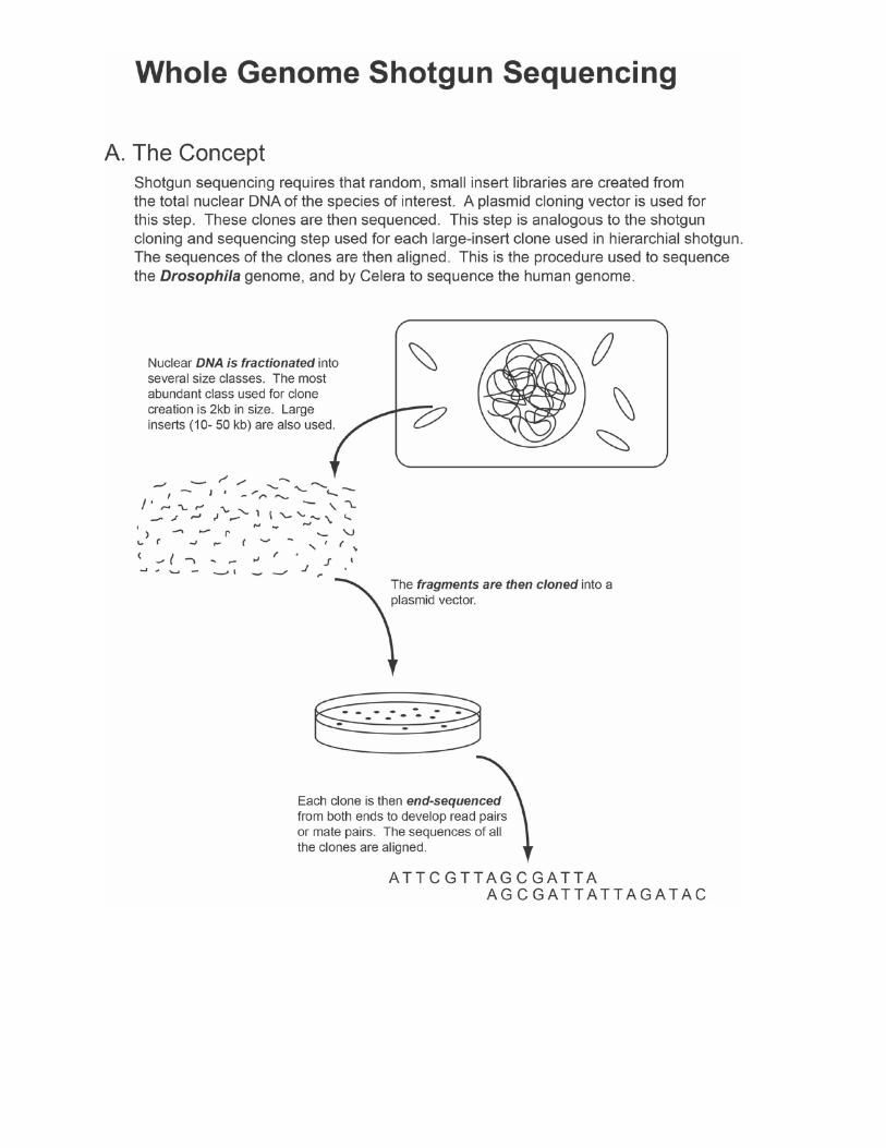
Whole Genome Shotgun Sequencing (WGS) • Hierarchical sequencing approach

o Begins with the physical map o Overlapping clones are shotgun cloned and sequenced

• WGS o Bypasses the mapping step

• Basic approach o Take nuclear DNA o Shear the DNA o Modify DNA by adding restriction site adaptors o Clone into plasmids

Plasmids are then directly sequenced Approach requires read-pairs

• Especially true because of the repetitive nature of complex genomes

WGS

• Proven very successful for smaller genomes o Essentially the only approach used to sequence smaller

genomes like bacteria • Is WGS useful for large, complex genomes?

o Initially consider a bold suggestion o Large public effort dedicated to hierarchical approach o Drosophila

Sequenced using the WGS approach

o Rice Early publications, not definitive Definitive reference genome developed from

hierarchialy shotgun sequencing Two different rice genomes sequenced using WGS

approach • Only developed a working draft though • Public hierarchical sequence available;

publication released in August 2005 WGS – Major Challenge 1

• Assembly of repetitive DNA is difficult o Retrotransposons (RNA mobile elements) o DNA transposons o Alu repeats (human) o Long and Short Interspersed Repeat (LINE and SINE)

elements o Microsatellites

• Solution o Use sequence data from 2, 10 and 50 kb clones

Data from fragments containing different types of sequences can be collected

Paired-end reads collected o Assembly Process

Repeat sequences are initially masked Overlaps of non-repeat sequences detected Contigs overlapped to create supercontigs

o Software available but is mostly useful to the developers Examples: Celera Assembler, Arcane, Phusion, Atlas

WGS – Major Challenge 2 • For the two sequences approaches • Assembly is a scale issue

o WGS approach Gigabytes of sequence data

o Hierarchical approach Magnitudes less

o On-going research focuses on developing new algorithms to handle and assembly the huge data sets generated by WGS

Mouse WGS Data

• 29.7 million reads • 7.4x coverage • Newer software • Assembled without mapping or clone data

o Human WGS had access to this data from the public project • 225,000 contigs

o Mean length = 25 kilobases in length • Super contig subset

o Mean length =16.9 megabases • 200 largest supercontigs

o Anchored using mapping data o Represents 96% (9187 Mb) of the euchromatic region of

genome

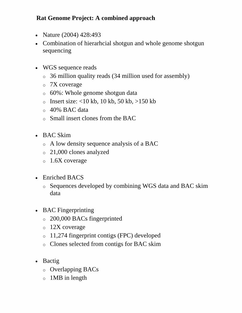
Rat Genome Project: A combined approach

• Nature (2004) 428:493 • Combination of hierarhcial shotgun and whole genome shotgun

sequencing

• WGS sequence reads o 36 million quality reads (34 million used for assembly) o 7X coverage o 60%: Whole genome shotgun data o Insert size: <10 kb, 10 kb, 50 kb, >150 kb o 40% BAC data o Small insert clones from the BAC

• BAC Skim

o A low density sequence analysis of a BAC o 21,000 clones analyzed o 1.6X coverage

• Enriched BACS

o Sequences developed by combining WGS data and BAC skim data

• BAC Fingerprinting

o 200,000 BACs fingerprinted o 12X coverage o 11,274 fingerprint contigs (FPC) developed o Clones selected from contigs for BAC skim

• Bactig

o Overlapping BACs o 1MB in length

• Superbactigs o Bactigs joined by paired-end reads o Mean = 5MB in length o 783 total for the genome

• Ultrabactigs

o Mean = 18 MB o 291 total for genome o Synteny data, marker data, and other data used to define the

ultrabactig

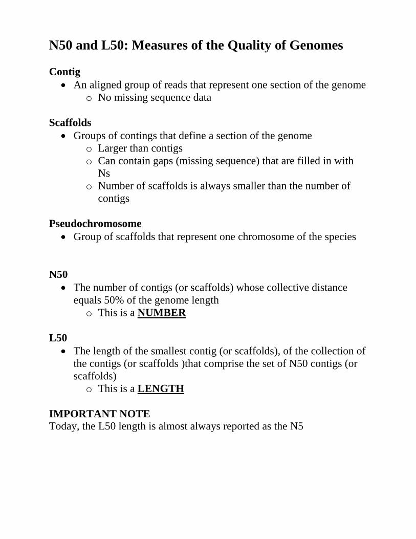
N50 and L50: Measures of the Quality of Genomes Contig

• An aligned group of reads that represent one section of the genome o No missing sequence data

Scaffolds

• Groups of contings that define a section of the genome o Larger than contigs o Can contain gaps (missing sequence) that are filled in with

Ns o Number of scaffolds is always smaller than the number of

contigs Pseudochromosome

• Group of scaffolds that represent one chromosome of the species N50

• The number of contigs (or scaffolds) whose collective distance equals 50% of the genome length o This is a NUMBER

L50

• The length of the smallest contig (or scaffolds), of the collection of the contigs (or scaffolds )that comprise the set of N50 contigs (or scaffolds) o This is a LENGTH

IMPORTANT NOTE Today, the L50 length is almost always reported as the N5

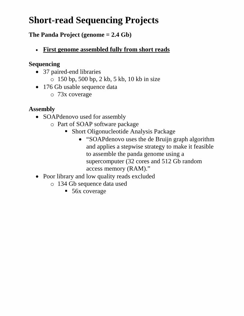
Short-read Sequencing Projects The Panda Project (genome = 2.4 Gb)

• First genome assembled fully from short reads Sequencing

• 37 paired-end libraries o 150 bp, 500 bp, 2 kb, 5 kb, 10 kb in size

• 176 Gb usable sequence data o 73x coverage

Assembly

• SOAPdenovo used for assembly o Part of SOAP software package

Short Oligonucleotide Analysis Package • “SOAPdenovo uses the de Bruijn graph algorithm

and applies a stepwise strategy to make it feasible to assemble the panda genome using a supercomputer (32 cores and 512 Gb random access memory (RAM).”

• Poor library and low quality reads excluded o 134 Gb sequence data used

56x coverage

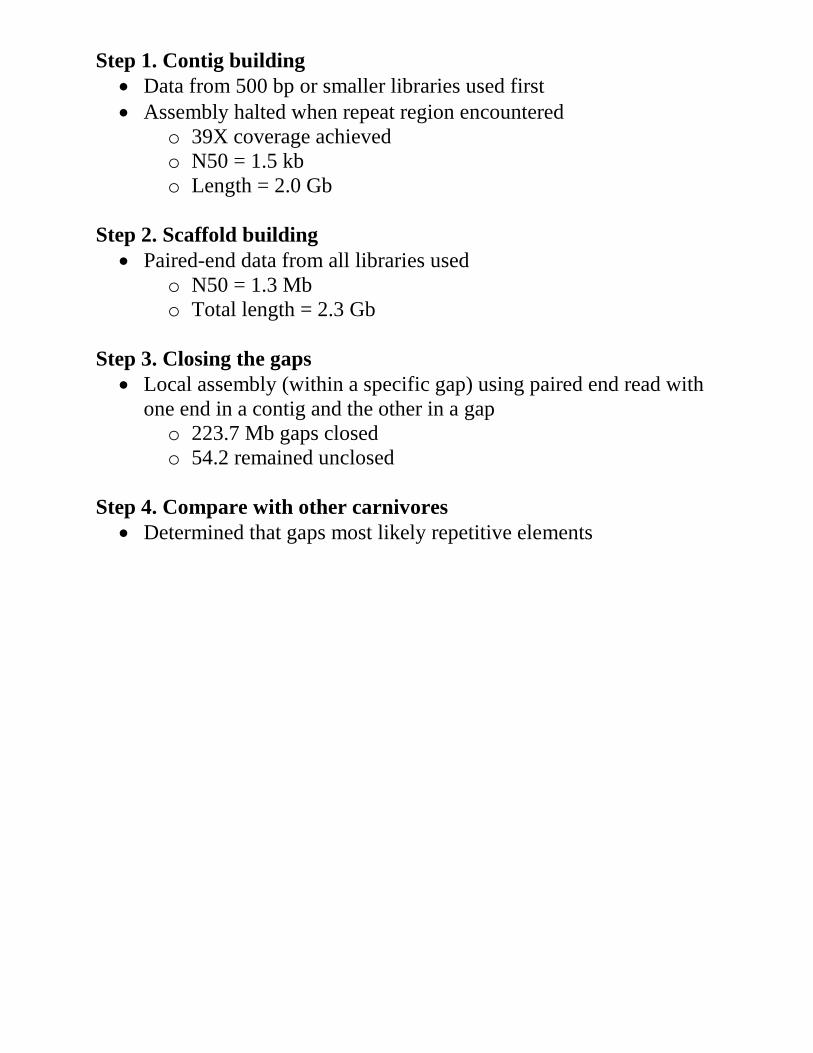
Step 1. Contig building • Data from 500 bp or smaller libraries used first • Assembly halted when repeat region encountered

o 39X coverage achieved o N50 = 1.5 kb o Length = 2.0 Gb

Step 2. Scaffold building

• Paired-end data from all libraries used o N50 = 1.3 Mb o Total length = 2.3 Gb

Step 3. Closing the gaps

• Local assembly (within a specific gap) using paired end read with one end in a contig and the other in a gap o 223.7 Mb gaps closed o 54.2 remained unclosed

Step 4. Compare with other carnivores

• Determined that gaps most likely repetitive elements

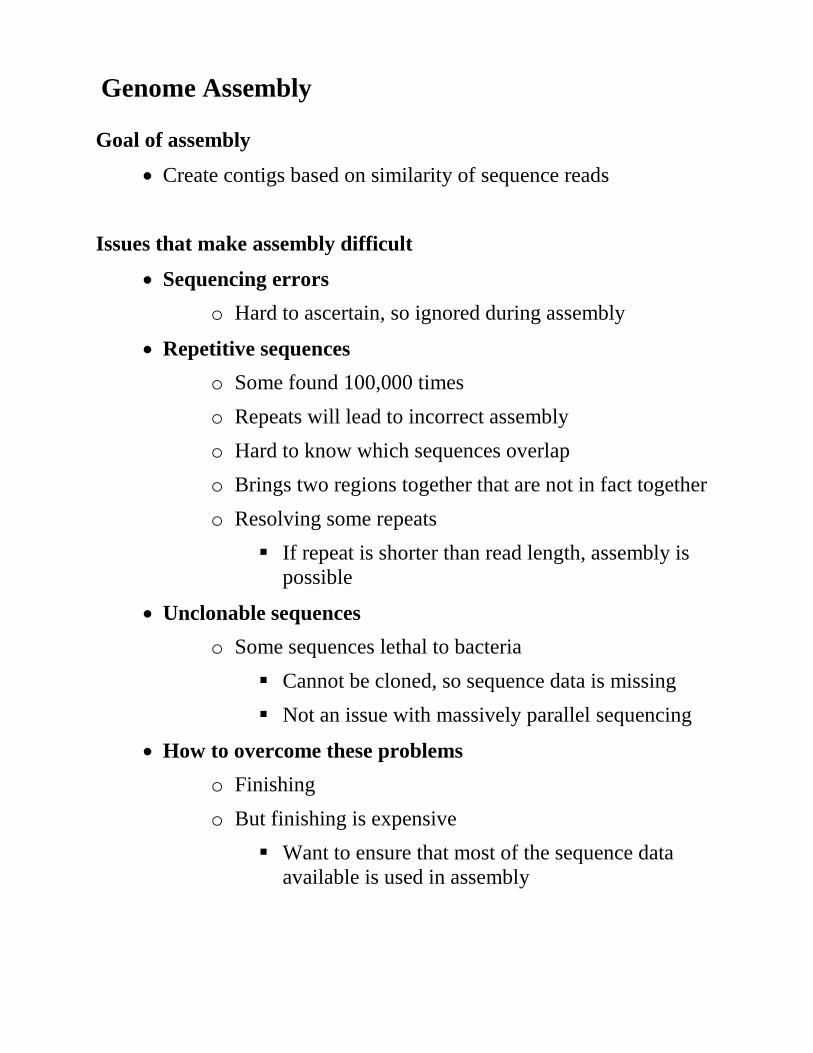
Genome Assembly Goal of assembly

• Create contigs based on similarity of sequence reads Issues that make assembly difficult

• Sequencing errors o Hard to ascertain, so ignored during assembly

• Repetitive sequences o Some found 100,000 times o Repeats will lead to incorrect assembly o Hard to know which sequences overlap o Brings two regions together that are not in fact together o Resolving some repeats

If repeat is shorter than read length, assembly is possible

• Unclonable sequences o Some sequences lethal to bacteria

Cannot be cloned, so sequence data is missing Not an issue with massively parallel sequencing

• How to overcome these problems o Finishing o But finishing is expensive

Want to ensure that most of the sequence data available is used in assembly

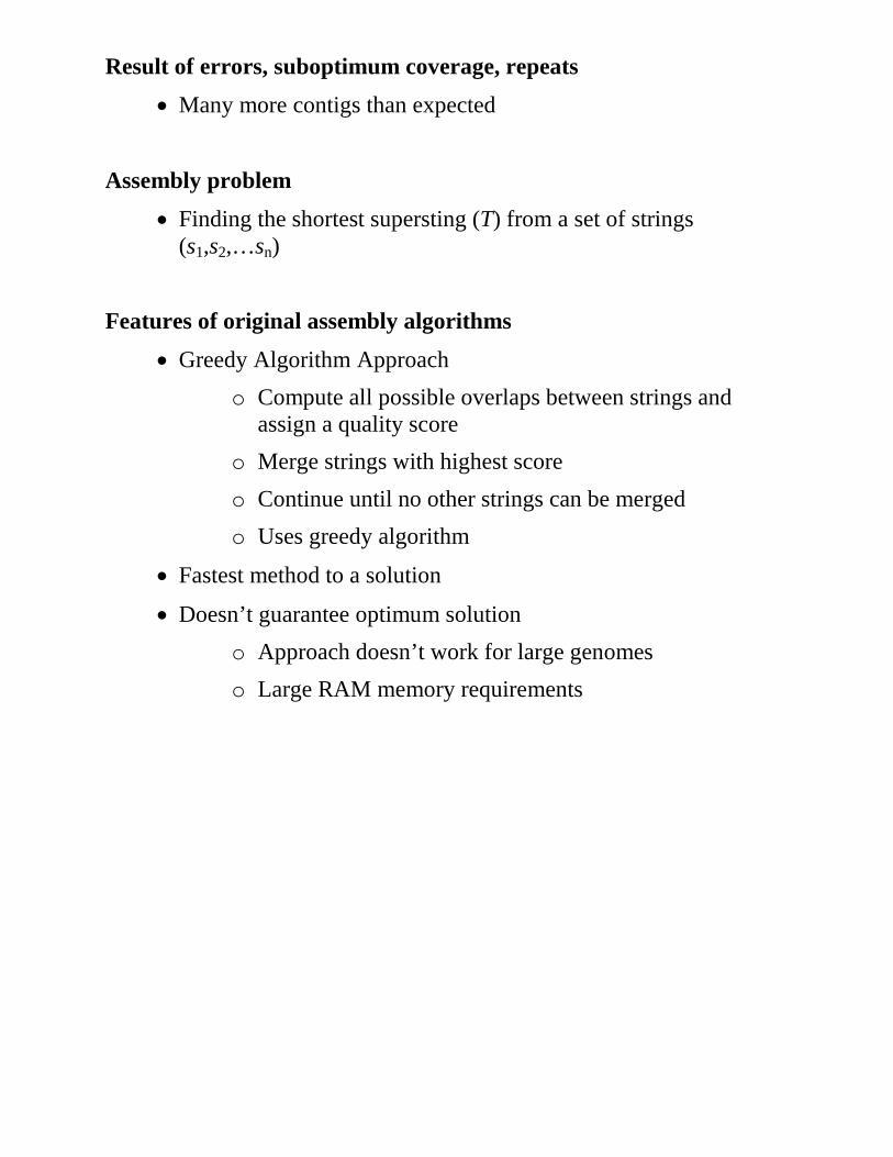
Result of errors, suboptimum coverage, repeats • Many more contigs than expected

Assembly problem

• Finding the shortest supersting (T) from a set of strings (s1,s2,…sn)

Features of original assembly algorithms

• Greedy Algorithm Approach o Compute all possible overlaps between strings and

assign a quality score o Merge strings with highest score o Continue until no other strings can be merged o Uses greedy algorithm

• Fastest method to a solution

• Doesn’t guarantee optimum solution o Approach doesn’t work for large genomes o Large RAM memory requirements

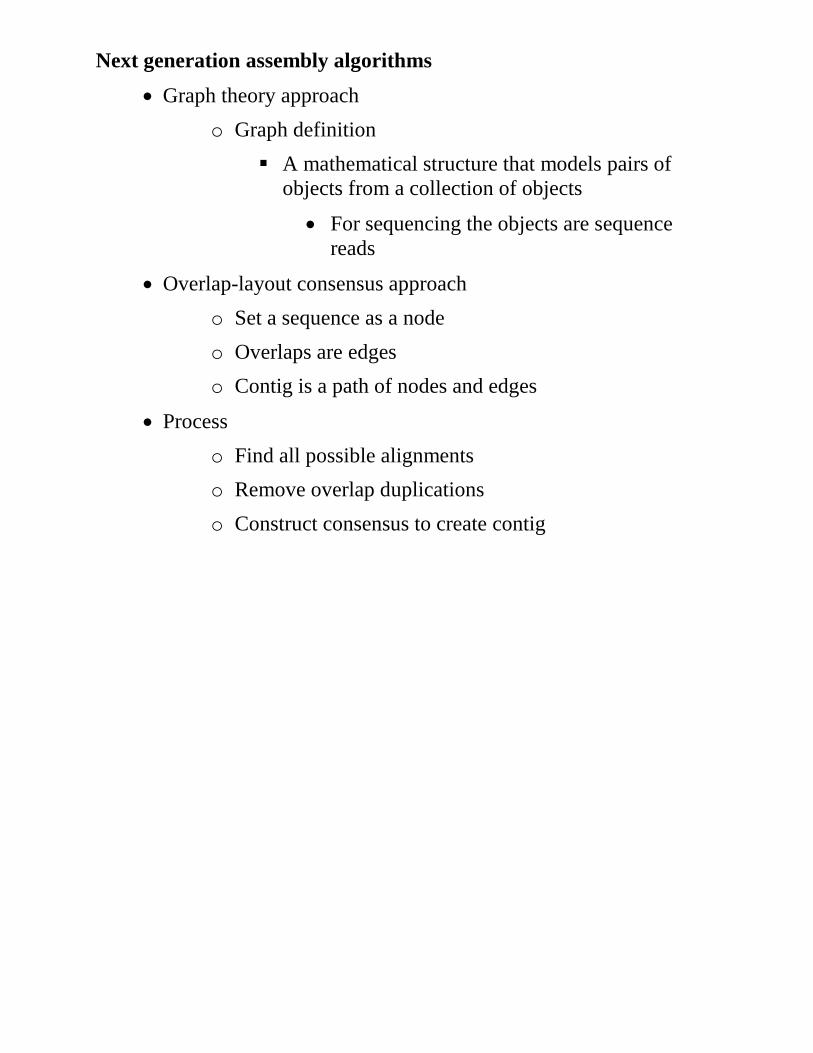
Next generation assembly algorithms • Graph theory approach

o Graph definition A mathematical structure that models pairs of

objects from a collection of objects

• For sequencing the objects are sequence reads

• Overlap-layout consensus approach o Set a sequence as a node o Overlaps are edges o Contig is a path of nodes and edges

• Process o Find all possible alignments o Remove overlap duplications o Construct consensus to create contig

ARACHNE Assembly Program Genome Research (2002) 12:177; Genome Research

(2003) 13:91 Data Preparation

1. Trim low quality sequences at ends of reads 2. Drop entire reads with low overall read scores 3. Trim vector sequences and any known contaminant sequences

Alignment of reads

1. Create table of k-mer (k=24) sequences a. each entry associated with a read and position in read 2. High frequency k-mers dropped (repetitive sequences)j 3. Read pairs sharing k-mers identified 4. Overlapping k-mers are merged 5. Shared k-mers extended 6. Alignments refined

Error Correction and Quality Scoring

1. Multiple alignments of overlapping reads created 2. Low frequency errors (20 C vs. 1 T) converted to consensus sequence 3. Insertions/deletions are corrected 4. Quality score attached to alignment

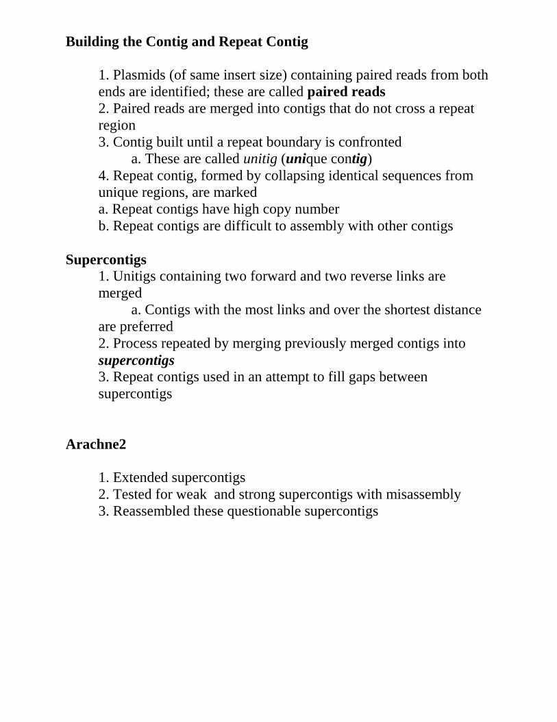
Building the Contig and Repeat Contig

1. Plasmids (of same insert size) containing paired reads from both ends are identified; these are called paired reads 2. Paired reads are merged into contigs that do not cross a repeat region 3. Contig built until a repeat boundary is confronted a. These are called unitig (unique contig) 4. Repeat contig, formed by collapsing identical sequences from unique regions, are marked

a. Repeat contigs have high copy number b. Repeat contigs are difficult to assembly with other contigs Supercontigs

1. Unitigs containing two forward and two reverse links are merged a. Contigs with the most links and over the shortest distance are preferred 2. Process repeated by merging previously merged contigs into supercontigs 3. Repeat contigs used in an attempt to fill gaps between supercontigs

Arachne2

1. Extended supercontigs 2. Tested for weak and strong supercontigs with misassembly 3. Reassembled these questionable supercontigs

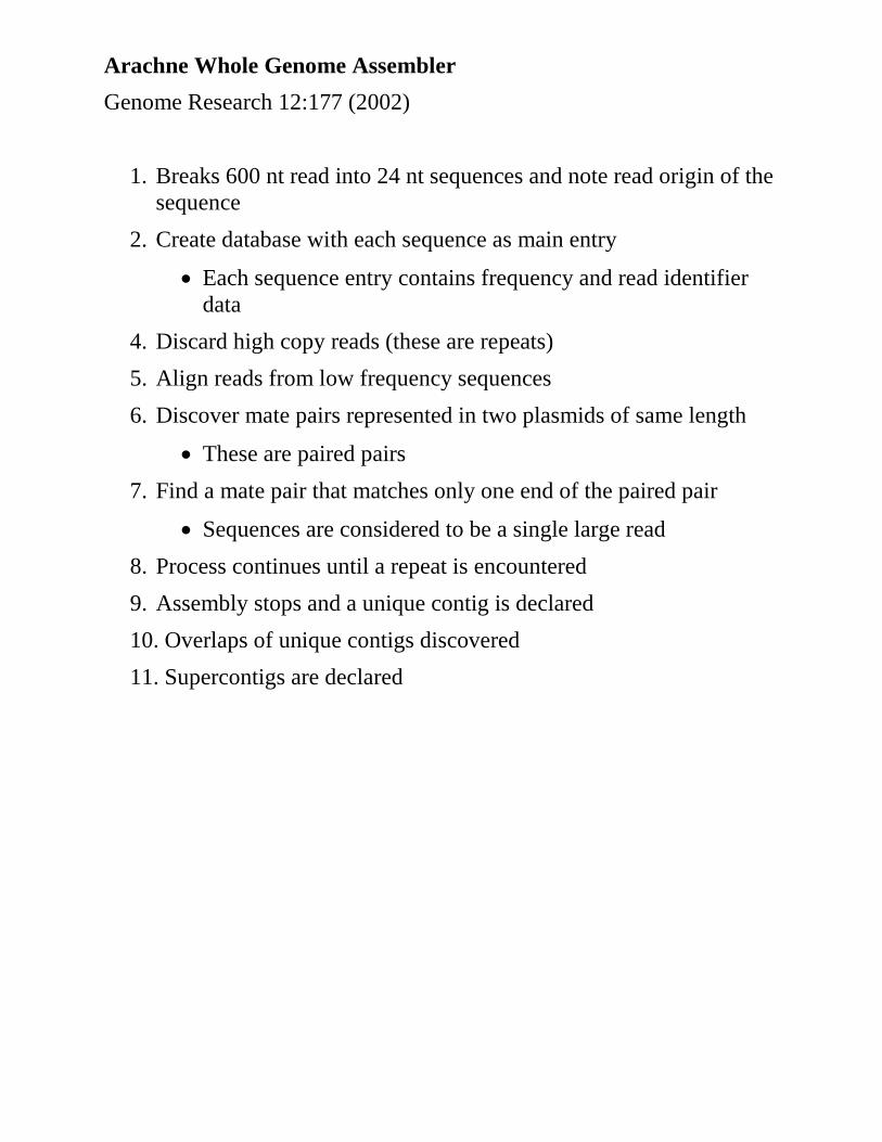
Arachne Whole Genome Assembler Genome Research 12:177 (2002)

1. Breaks 600 nt read into 24 nt sequences and note read origin of the sequence

2. Create database with each sequence as main entry

• Each sequence entry contains frequency and read identifier data

4. Discard high copy reads (these are repeats) 5. Align reads from low frequency sequences 6. Discover mate pairs represented in two plasmids of same length

• These are paired pairs 7. Find a mate pair that matches only one end of the paired pair

• Sequences are considered to be a single large read 8. Process continues until a repeat is encountered 9. Assembly stops and a unique contig is declared 10. Overlaps of unique contigs discovered 11. Supercontigs are declared

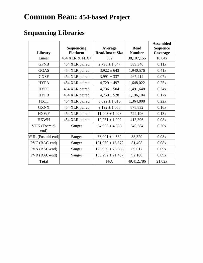
Common Bean: 454-based Project Sequencing Libraries

Library Sequencing

Platform Average

Read/Insert Size Read

Number

Assembled Sequence Coverage

Linear 454 XLR & FLX+ 362 38,107,155 18.64x GPNB 454 XLR paired 2,798 ± 1,047 589,346 0.11x GGAS 454 XLR paired 3,922 ± 643 1,940,576 0.41x GXSF 454 XLR paired 3,991 ± 337 467,414 0.07x HYFA 454 XLR paired 4,729 ± 497 1,648,022 0.25x HYFC 454 XLR paired 4,736 ± 504 1,491,648 0.24x HYFB 454 XLR paired 4,759 ± 528 1,196,104 0.17x HXTI 454 XLR paired 8,022 ± 1,016 1,364,808 0.22x GXNX 454 XLR paired 9,192 ± 1,058 878,832 0.16x HXWF 454 XLR paired 11,903 ± 1,928 724,196 0.13x HXWH 454 XLR paired 12,231 ± 1,902 413,396 0.08x

VUK (Fosmid-end)

Sanger 34,956 ± 4,536 240,384 0.20x

VUL (Fosmid-end) Sanger 36,001 ± 4,632 88,320 0.08x PVC (BAC-end) Sanger 121,960 ± 16,572 81,408 0.08x PVA (BAC-end) Sanger 126,959 ± 25,658 89,017 0.09x PVB (BAC-end) Sanger 135,292 ± 21,487 92,160 0.09x

Total N/A 49,412,786 21.02x

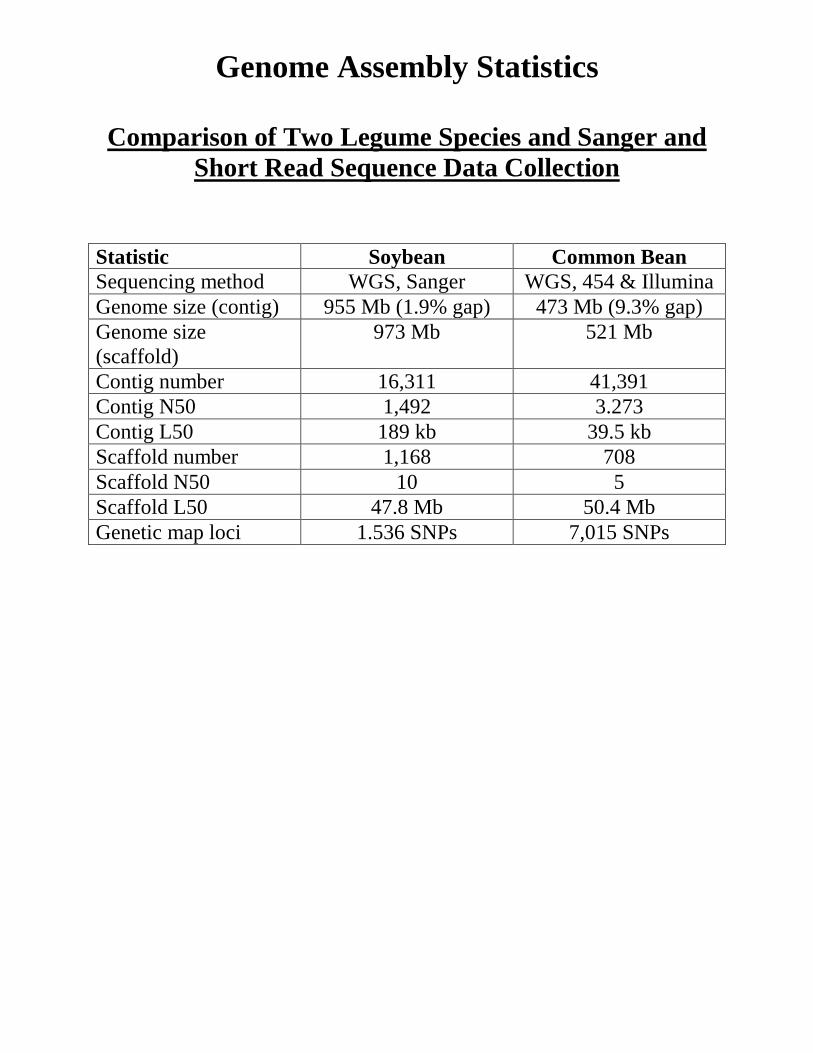
Genome Assembly Statistics

Comparison of Two Legume Species and Sanger and Short Read Sequence Data Collection

Statistic Soybean Common Bean Sequencing method WGS, Sanger WGS, 454 & Illumina Genome size (contig) 955 Mb (1.9% gap) 473 Mb (9.3% gap) Genome size (scaffold)

973 Mb 521 Mb

Contig number 16,311 41,391 Contig N50 1,492 3.273 Contig L50 189 kb 39.5 kb Scaffold number 1,168 708 Scaffold N50 10 5 Scaffold L50 47.8 Mb 50.4 Mb Genetic map loci 1.536 SNPs 7,015 SNPs

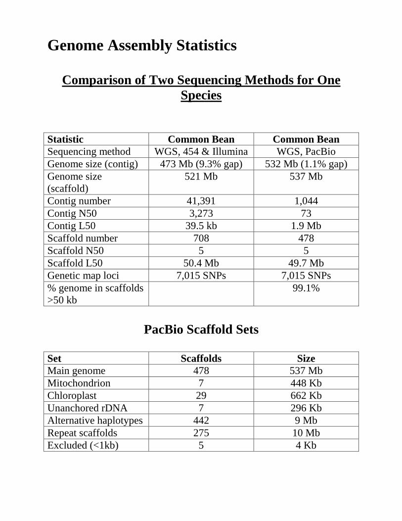
Genome Assembly Statistics

Comparison of Two Sequencing Methods for One

Species Statistic Common Bean Common Bean Sequencing method WGS, 454 & Illumina WGS, PacBio Genome size (contig) 473 Mb (9.3% gap) 532 Mb (1.1% gap) Genome size (scaffold)

521 Mb 537 Mb

Contig number 41,391 1,044 Contig N50 3,273 73 Contig L50 39.5 kb 1.9 Mb Scaffold number 708 478 Scaffold N50 5 5 Scaffold L50 50.4 Mb 49.7 Mb Genetic map loci 7,015 SNPs 7,015 SNPs % genome in scaffolds >50 kb

99.1%

PacBio Scaffold Sets

Set Scaffolds Size Main genome 478 537 Mb Mitochondrion 7 448 Kb Chloroplast 29 662 Kb Unanchored rDNA 7 296 Kb Alternative haplotypes 442 9 Mb Repeat scaffolds 275 10 Mb Excluded (<1kb) 5 4 Kb

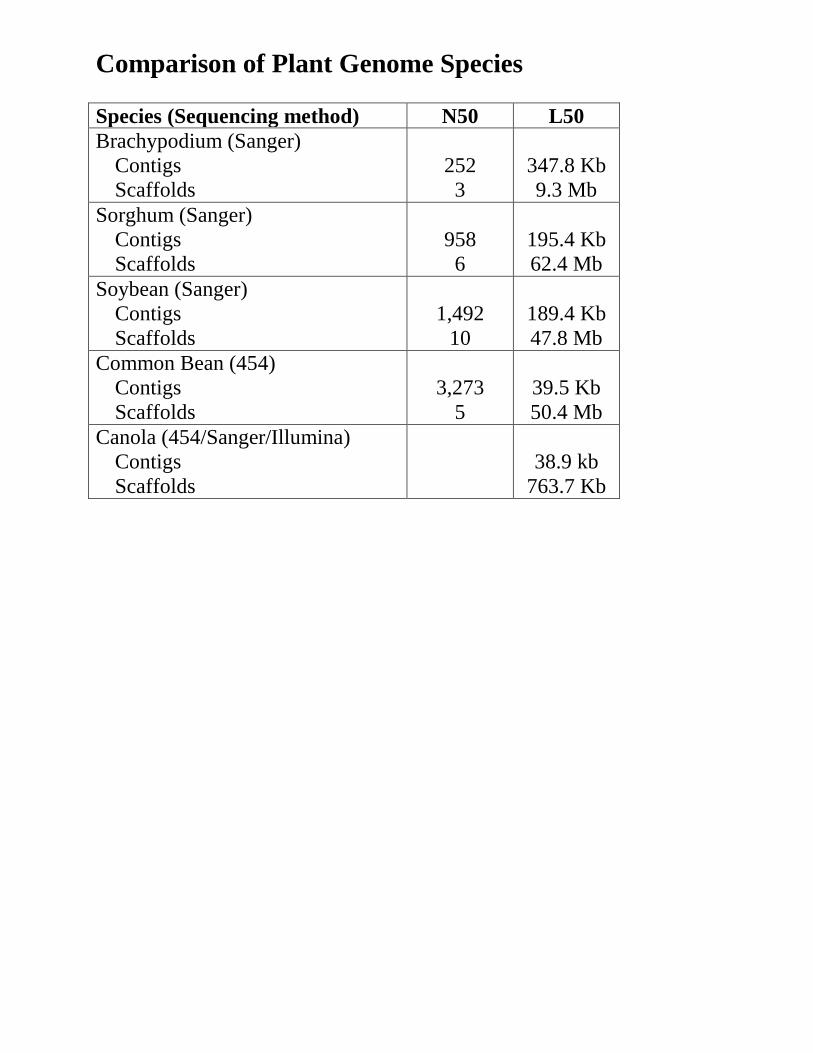
Comparison of Plant Genome Species Species (Sequencing method) N50 L50 Brachypodium (Sanger)

Contigs Scaffolds

252 3

347.8 Kb 9.3 Mb

Sorghum (Sanger) Contigs Scaffolds

958 6

195.4 Kb 62.4 Mb

Soybean (Sanger) Contigs Scaffolds

1,492

10

189.4 Kb 47.8 Mb

Common Bean (454) Contigs Scaffolds

3,273

5

39.5 Kb 50.4 Mb

Canola (454/Sanger/Illumina) Contigs Scaffolds

38.9 kb

763.7 Kb

Sca�old AssemblyBuilding a Sca�old Using Paired-end Reads of Di�erent Sized Sequences

40-kbread

Step 1: Build a contig with overlapping2-kb paired-end reads

Step 2: Link two contigs with10-kb paired-end reads

Step 3: Link three 10-kb contigs with40-kb paired-end reads

Step 4: Link two 40-kb contigs with100-kb BAC end sequences (BES)

Step 5: Here link two100-kb BAC sized contigs witha 40-kb paired-end read; other sized readscan also be used for this linking

Step 6: Continue linking larger blocks of sequences until the block can not be linked with another block.This block is de�ned as a sca�old.

2-kbread

10-kbread

40-kbread

BESread

40-kbread

40-kbread

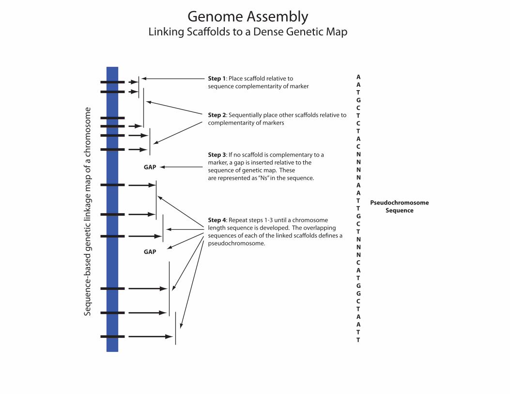
Genome AssemblyLinking Sca�olds to a Dense Genetic Map

Sequ

ence

-bas

ed g

enet

ic li

nkag

e m

ap o

f a c

hrom

osom

eStep 1: Place sca�old relative tosequence complementarity of marker

Step 2: Sequentially place other sca�olds relative tocomplementarity of markers

Step 3: If no sca�old is complementary to a marker, a gap is inserted relative to thesequence of genetic map. These are represented as “Ns” in the sequence.

Step 4: Repeat steps 1-3 until a chromosomelength sequence is developed. The overlappingsequences of each of the linked sca�olds de�nes a pseudochromosome.

GAP

GAP

AATGCTCTACNNNNAATTGCTNNNCATGGCTAATT

PseudochromosomeSequence

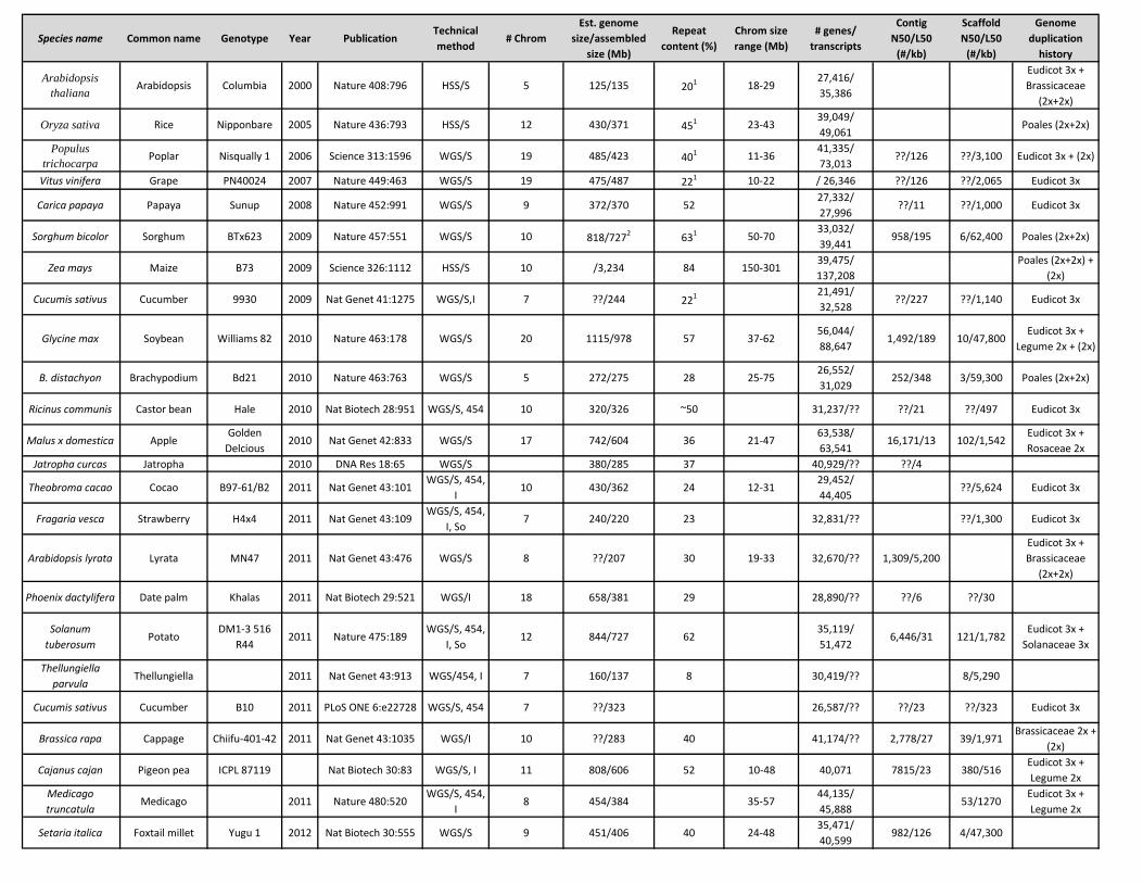
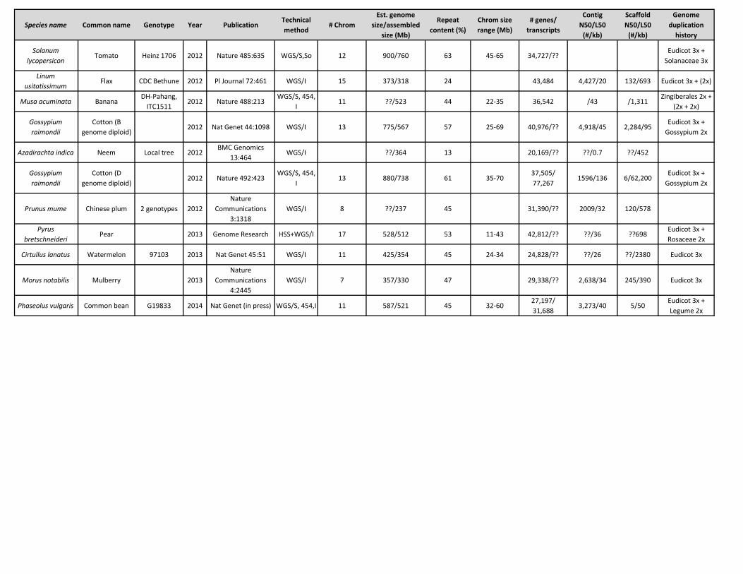
Species name Common name Genotype Year PublicationTechnical method

# ChromEst. genome

size/assembled size (Mb)

Repeat content (%)

Chrom size range (Mb)

# genes/ transcripts

Contig N50/L50

(#/kb)

Scaffold N50/L50

(#/kb)

Genome duplication

history

Arabidopsis thaliana Arabidopsis Columbia 2000 Nature 408:796 HSS/S 5 125/135 201 18-29

27,416/ 35,386

Eudicot 3x + Brassicaceae

(2x+2x)

Oryza sativa Rice Nipponbare 2005 Nature 436:793 HSS/S 12 430/371 451 23-4339,049/ 49,061

Poales (2x+2x)

Populus trichocarpa Poplar Nisqually 1 2006 Science 313:1596 WGS/S 19 485/423 401 11-36

41,335/ 73,013

??/126 ??/3,100 Eudicot 3x + (2x)

Vitus vinifera Grape PN40024 2007 Nature 449:463 WGS/S 19 475/487 221 10-22 / 26,346 ??/126 ??/2,065 Eudicot 3x

Carica papaya Papaya Sunup 2008 Nature 452:991 WGS/S 9 372/370 5227,332/ 27,996

??/11 ??/1,000 Eudicot 3x

Sorghum bicolor Sorghum BTx623 2009 Nature 457:551 WGS/S 10 818/7272 631 50-7033,032/ 39,441

958/195 6/62,400 Poales (2x+2x)

Zea mays Maize B73 2009 Science 326:1112 HSS/S 10 /3,234 84 150-30139,475/ 137,208

Poales (2x+2x) + (2x)

Cucumis sativus Cucumber 9930 2009 Nat Genet 41:1275 WGS/S,I 7 ??/244 221 21,491/ 32,528

??/227 ??/1,140 Eudicot 3x

Glycine max Soybean Williams 82 2010 Nature 463:178 WGS/S 20 1115/978 57 37-6256,044/ 88,647

1,492/189 10/47,800Eudicot 3x +

Legume 2x + (2x)

B. distachyon Brachypodium Bd21 2010 Nature 463:763 WGS/S 5 272/275 28 25-7526,552/ 31,029

252/348 3/59,300 Poales (2x+2x)

Ricinus communis Castor bean Hale 2010 Nat Biotech 28:951 WGS/S, 454 10 320/326 ~50 31,237/?? ??/21 ??/497 Eudicot 3x

Malus x domestica AppleGolden

Delcious2010 Nat Genet 42:833 WGS/S 17 742/604 36 21-47

63,538/ 63,541

16,171/13 102/1,542Eudicot 3x + Rosaceae 2x

Jatropha curcas Jatropha 2010 DNA Res 18:65 WGS/S 380/285 37 40,929/?? ??/4

Theobroma cacao Cocao B97-61/B2 2011 Nat Genet 43:101WGS/S, 454,

I10 430/362 24 12-31

29,452/ 44,405

??/5,624 Eudicot 3x

Fragaria vesca Strawberry H4x4 2011 Nat Genet 43:109WGS/S, 454,

I, So7 240/220 23 32,831/?? ??/1,300 Eudicot 3x

Arabidopsis lyrata Lyrata MN47 2011 Nat Genet 43:476 WGS/S 8 ??/207 30 19-33 32,670/?? 1,309/5,200Eudicot 3x + Brassicaceae

(2x+2x)

Phoenix dactylifera Date palm Khalas 2011 Nat Biotech 29:521 WGS/I 18 658/381 29 28,890/?? ??/6 ??/30

Solanum tuberosum

PotatoDM1-3 516

R442011 Nature 475:189

WGS/S, 454, I, So

12 844/727 6235,119/ 51,472

6,446/31 121/1,782Eudicot 3x +

Solanaceae 3x

Thellungiella parvula

Thellungiella 2011 Nat Genet 43:913 WGS/454, I 7 160/137 8 30,419/?? 8/5,290

Cucumis sativus Cucumber B10 2011 PLoS ONE 6:e22728 WGS/S, 454 7 ??/323 26,587/?? ??/23 ??/323 Eudicot 3x

Brassica rapa Cappage Chiifu-401-42 2011 Nat Genet 43:1035 WGS/I 10 ??/283 40 41,174/?? 2,778/27 39/1,971Brassicaceae 2x +

(2x)

Cajanus cajan Pigeon pea ICPL 87119 Nat Biotech 30:83 WGS/S, I 11 808/606 52 10-48 40,071 7815/23 380/516Eudicot 3x + Legume 2x

Medicago truncatula

Medicago 2011 Nature 480:520WGS/S, 454,

I8 454/384 35-57

44,135/ 45,888

53/1270Eudicot 3x + Legume 2x

Setaria italica Foxtail millet Yugu 1 2012 Nat Biotech 30:555 WGS/S 9 451/406 40 24-4835,471/ 40,599

982/126 4/47,300

Species name Common name Genotype Year PublicationTechnical method

# ChromEst. genome

size/assembled size (Mb)

Repeat content (%)

Chrom size range (Mb)

# genes/ transcripts

Contig N50/L50

(#/kb)

Scaffold N50/L50

(#/kb)

Genome duplication

history

Solanum lycopersicon

Tomato Heinz 1706 2012 Nature 485:635 WGS/S,So 12 900/760 63 45-65 34,727/??Eudicot 3x +

Solanaceae 3x

Linum usitatissimum

Flax CDC Bethune 2012 Pl Journal 72:461 WGS/I 15 373/318 24 43,484 4,427/20 132/693 Eudicot 3x + (2x)

Musa acuminata BananaDH-Pahang,

ITC15112012 Nature 488:213

WGS/S, 454, I

11 ??/523 44 22-35 36,542 /43 /1,311Zingiberales 2x +

(2x + 2x)

Gossypium raimondii

Cotton (B genome diploid)

2012 Nat Genet 44:1098 WGS/I 13 775/567 57 25-69 40,976/?? 4,918/45 2,284/95Eudicot 3x +

Gossypium 2x

Azadirachta indica Neem Local tree 2012BMC Genomics

13:464WGS/I ??/364 13 20,169/?? ??/0.7 ??/452

Gossypium raimondii

Cotton (D genome diploid)

2012 Nature 492:423WGS/S, 454,

I13 880/738 61 35-70

37,505/ 77,267

1596/136 6/62,200Eudicot 3x +

Gossypium 2x

Prunus mume Chinese plum 2 genotypes 2012Nature

Communications 3:1318

WGS/I 8 ??/237 45 31,390/?? 2009/32 120/578

Pyrus bretschneideri

Pear 2013 Genome Research HSS+WGS/I 17 528/512 53 11-43 42,812/?? ??/36 ??698Eudicot 3x + Rosaceae 2x

Cirtullus lanatus Watermelon 97103 2013 Nat Genet 45:51 WGS/I 11 425/354 45 24-34 24,828/?? ??/26 ??/2380 Eudicot 3x

Morus notabilis Mulberry 2013Nature

Communications 4:2445

WGS/I 7 357/330 47 29,338/?? 2,638/34 245/390 Eudicot 3x

Phaseolus vulgaris Common bean G19833 2014 Nat Genet (in press) WGS/S, 454,I 11 587/521 45 32-6027,197/ 31,688

3,273/40 5/50Eudicot 3x + Legume 2x

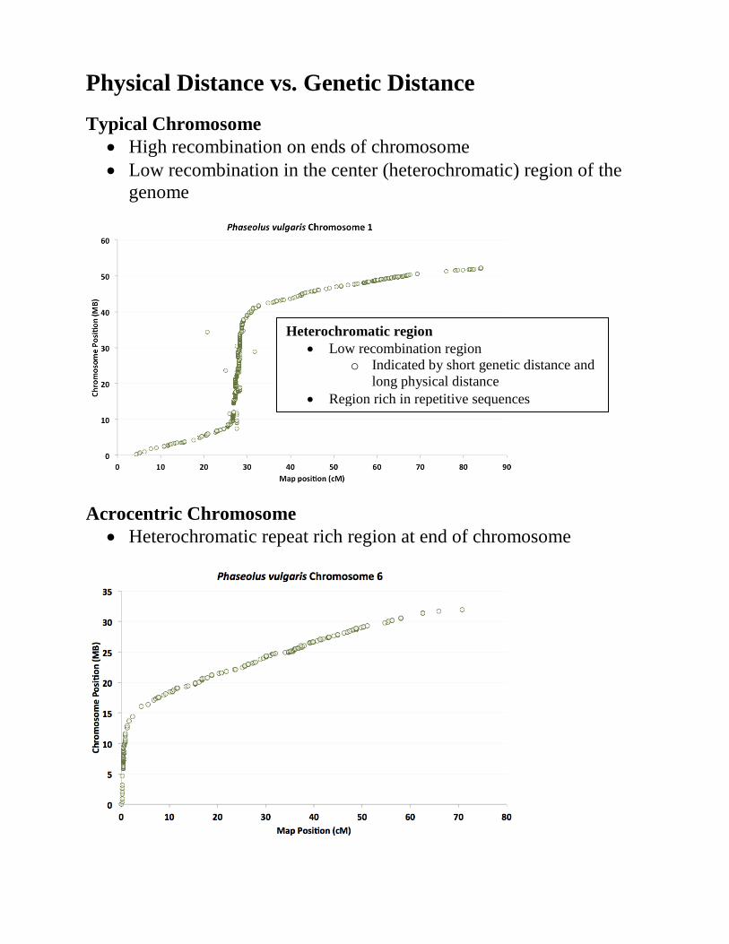
Physical Distance vs. Genetic Distance Typical Chromosome

• High recombination on ends of chromosome • Low recombination in the center (heterochromatic) region of the

genome

Acrocentric Chromosome • Heterochromatic repeat rich region at end of chromosome

Heterochromatic region • Low recombination region

o Indicated by short genetic distance and long physical distance

• Region rich in repetitive sequences