Embed Size (px)
Citation preview
Genetic Algorithm for Shipping Route Estimation
with Long-Range Tracking Data
Andrea Pelizzari
Automatic reconstruction of shipping routes based
on the historical ship positions for Maritime Safety
Applications.
Trabalho de Projeto apresentado como requisito parcial para
obtenção do grau de Mestre em Gestão de Informação


Genetic Algorithm for Shipping Route Estimation with Long-Range Tracking Data
Automatic reconstruction of a shipping route based on the historical ship positions for Maritime Safety Applications
20
15
Andrea Pelizzari


i
NOVA Information Management School
Instituto Superior de Estatística e Gestão de Informação
Universidade Nova de Lisboa
GENETIC ALGORITHM FOR SHIPPING ROUTE ESTIMATION WITH
LONG-RANGE TRACKING DATA
by
Andrea Pelizzari
Trabalho de Projeto apresentado como requisito parcial para a obtenção do grau de Mestre em
Gestão de Informação, Especialização em Business Intelligence
Supervisor: Prof. Leonardo Vanneschi
November 2015

ii
Ai miei genitori, Mimma e Cesare,
per i valori e la forza che mi hanno saputo trasmettere.
iii
ACKNOWLEDGEMENTS
It would be hard to do Big Data without the data and I wish to thank the Organizations that gave me
access to their valuable digital archives and systems and therefore the possibility to execute this
project: the European Maritime Safety Agency (EMSA), the Norwegian Coastal Administration
“Kystverket”, the Italian Coast Guard “Guardia Costiera Italiana”, the Maltese Maritime Authority
“Transport Malta”, and the company exactEarth Ltd.
A sincere appreciation to my colleagues at EMSA: Marin Chintoan-Uta, the seafarer who learned how
to do IT, for his valuable insights and expert assessment of the project outcome; Leendert Bal and
the Agency Management for their support to my study efforts; Lawrence Sciberras and Dario Cau, for
their well-placed connections; Simone Balboni and his Team, for the great computer infrastructure
they set up and operate; Marton Papp, for his decoding skills.
Un sentito ringraziamento al Prof. Leonardo Vanneschi per la sua competenza, la sua grande
disponibilità e per avermi consigliato di tornare sui banchi di scuola e seguire questo corso. Un grazie
anche al C.V. Leopoldo Manna, Walter Conti e agli altri colleghi della Guardia Costiera per la loro
gentilezza e, soprattutto, per il lavoro egregio e il grande esempio di umanità e spirito di sacrifício
che dimostrano tutti i giorni sulle acque del Mediterraneo.
I also wish to thank: Ivan Sammut, Harald Åsheim, Simon Chesworth, for the authorization to use
their data, and Michele Vespe, for his references on this topic.
I am very lucky to develop software technology in a time when amazing resources are available to
anyone working with a computer and an Internet connection. I wish to thank all the great engineers,
researchers, developers and technicians at: the Evolutionary Computation Laboratory at George
Mason University, for the ECJ library that helps a machine learning how to cross the Atlantic; Google
Inc., for their search engine that makes the literature review a doable task even for me, the Google
Drive that backs everything up, and the Google Earth application for drawing bizarre zigzagging tracks
on a nice geographical map background; MySQL, for the database that managed to index 700 million
positions in the blink of an eye; the Eclipse Foundation, for the very productive software
development environment; Github Inc., for version control and my peace of mind; Microsoft Inc. for
their Office suite (after 20 years Word is now ok for writing a thesis… well kind of) and their GIS
layers; the Danish Maritime Authority DMA, for their AISlib that shows how sharing technology is
good public service; minigeo, for its ultra-simplicity; jGraph Ltd. for their great online drawing tool
draw.io.
Finally I say “Grazie!” and “Obrigado!” to my European kids Anna, Francesco, and Isabella, my artistic
sister Alessandra, the olive oil enthusiasts Augusta and Antonino, and to my friends, for their love,
affection and support during the highs and lows of my life and this Master project: Paolo, Gigio,
Stefano, Cristiano, Camilla, Leopoldo, Sandro, Isa, Joost, Adinda, Rosário, José, Ricardo, Rui, and
Nuno.
iv
ABSTRACT
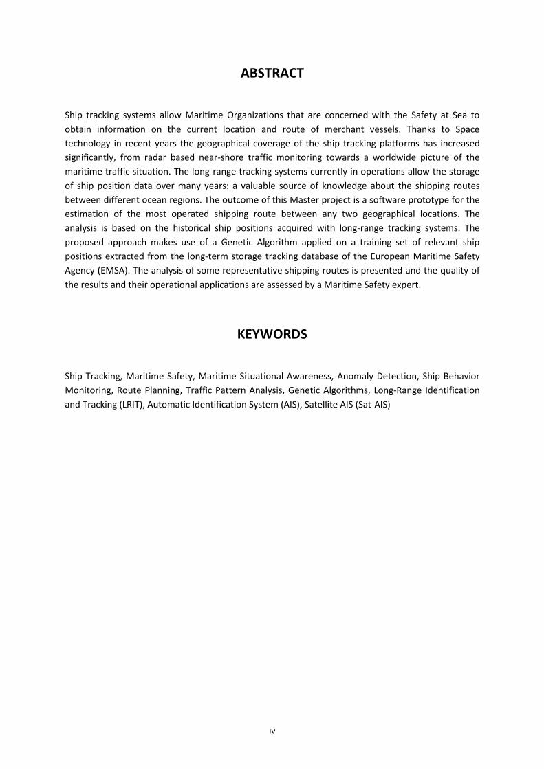
Ship tracking systems allow Maritime Organizations that are concerned with the Safety at Sea to
obtain information on the current location and route of merchant vessels. Thanks to Space
technology in recent years the geographical coverage of the ship tracking platforms has increased
significantly, from radar based near-shore traffic monitoring towards a worldwide picture of the
maritime traffic situation. The long-range tracking systems currently in operations allow the storage
of ship position data over many years: a valuable source of knowledge about the shipping routes
between different ocean regions. The outcome of this Master project is a software prototype for the
estimation of the most operated shipping route between any two geographical locations. The
analysis is based on the historical ship positions acquired with long-range tracking systems. The
proposed approach makes use of a Genetic Algorithm applied on a training set of relevant ship
positions extracted from the long-term storage tracking database of the European Maritime Safety
Agency (EMSA). The analysis of some representative shipping routes is presented and the quality of
the results and their operational applications are assessed by a Maritime Safety expert.
KEYWORDS
Ship Tracking, Maritime Safety, Maritime Situational Awareness, Anomaly Detection, Ship Behavior
Monitoring, Route Planning, Traffic Pattern Analysis, Genetic Algorithms, Long-Range Identification
and Tracking (LRIT), Automatic Identification System (AIS), Satellite AIS (Sat-AIS)
v
RESUMO
Os sistemas de monitorização do tráfego de navios permitem às Autoridades Marítimas,
responsáveis da segurança da navegação, conhecer a posição actual e as rotas da frota mercante.
Através da tecnologia espacial, o alcance geográfico das plataformas de monitorização de navios tem
aumentado de uma maneira significativa nos últimos anos. A inicial monitorização do tráfego com
radar e perto da costa transformou-se no conhecimento da situação da navegação marítima a nível
global. Os sistemas de monitorização de longo alcance atualmente operativos permitem a
armazenagem dos dados de posição de navios durante muitos anos: uma fonte valiosa de
conhecimento das rotas de navegação da frota comercial. Este projecto de Mestrado tem o objectivo
de desenvolver um protótipo de software para a estimativa da rota mais navegada entre dois
quaisquer pontos geográficos. A análise baseia-se nas posições históricas de navios, adquiridas com
sistemas de monitorização de longo alcance. A abordagem proposta utiliza um Algoritmo Genético
aplicado a um conjunto de treino de posições de navios extraídas das bases de dados de longo prazo
da Agência Europeia de Segurança Marítima (EMSA). Apresenta-se a análise de algumas rotas
comerciais representativas e a avaliação da qualidade dos resultados e das possíveis aplicações
operacionais feita por um perito de Segurança Marítima.
PALAVRAS-CHAVE
Monitorização de navios, segurança marítima, conhecimento da situação marítima, detecção de
anomalias, monitorização do comportamento de navios, planeamento de rota, análise de padrões de
tráfego, algoritmos genéticos, Long-Range Identification and Tracking (LRIT), Automatic Identification
System (AIS), AIS por satélite (Sat-AIS)

vi
INDEX
1. Introduction .................................................................................................................. 1
1.1. Maritime Safety, Ship Tracking, and Shipping Routes .......................................... 2
1.2. Project Objectives .................................................................................................. 3
1.3. Relevant Activities and Projects ............................................................................ 4
1.4. Document Structure .............................................................................................. 4
2. Literature Review ......................................................................................................... 6
3. Methodology ................................................................................................................ 8
3.1. The Shipping Route Estimation System ................................................................. 8
3.2. Data Collection ...................................................................................................... 9
3.3. Data Pre-Processing ............................................................................................. 11
3.4. Algorithm Selection and Implementation ........................................................... 12
3.5. Machine Learning Algorithm ............................................................................... 13
3.6. Algorithm Validation ........................................................................................... 13
4. The Data ...................................................................................................................... 14
4.1. Long-Range Identification and Tracking (LRIT) .................................................... 14
4.1.1. Characteristics of the LRIT Data ................................................................... 14
4.2. Sat-AIS .................................................................................................................. 15
4.2.1. Characteristics of the Sat-AIS Data ............................................................... 15
5. Data Pre-Processing .................................................................................................... 16
5.1. Extract, Transform and Load (ETL) ...................................................................... 16
5.1.1. AIS Message Datasets ................................................................................... 17
5.1.2. Load into Staging Area.................................................................................. 17
5.2. The Shipping Route Data Mart ............................................................................ 18
5.2.1. Ship Tracks .................................................................................................... 19
5.2.2. Time Normalization ...................................................................................... 21
6. The Genetic Algorithm ................................................................................................ 22
6.1. Description of Genetic Algorithms ...................................................................... 22
6.2. Shipping Route Modelling ................................................................................... 23
6.3. Representation of a Ship Track ........................................................................... 25
6.3.1. Timestamps and list of segments ................................................................. 26
6.3.2. Crossover and Mutation of Tracks ............................................................... 27
6.4. The Search for Fitness ......................................................................................... 30
6.4.1. Distance to the ship positions ...................................................................... 31
vii
6.4.2. Variance of the distance to the ship positions ............................................. 34
6.4.3. Ship Position Coverage ................................................................................. 35
6.4.4. Distance to destination ................................................................................ 36
6.4.5. Change of Heading ....................................................................................... 37
6.5. Building Up the Fitness ........................................................................................ 38
6.5.1. Setting the Weighting Factors ...................................................................... 40
6.6. ECJ: an Evolutionary Computation Research System .......................................... 40
6.6.1. Genetic Algorithm Configuration Parameters.............................................. 40
7. Results......................................................................................................................... 42
7.1. Shipping Route Estimation in Practice ................................................................ 42
7.1.1. Performance ................................................................................................. 44
7.2. Use Case Scenarios .............................................................................................. 44
7.2.1. Lanzarote-Natal Route ................................................................................. 44
7.2.2. Channel-Nova Scotia Route .......................................................................... 48
7.2.3. Red Sea-Gulf of Aden Route ......................................................................... 52
7.3. Expert Assessment .............................................................................................. 55
7.4. Maritime Safety Applications .............................................................................. 55
7.4.1. Ship Monitoring and Alerting ....................................................................... 56
7.4.2. Route Planning ............................................................................................. 56
7.4.3. Route Pattern Analysis ................................................................................. 57
8. Conclusions and Future Work .................................................................................... 58
8.1. Future Development ........................................................................................... 59
9. Bibliography ................................................................................................................ 60
10. Annexes ................................................................................................................ 61
10.1. AIS Messages ................................................................................................. 61
10.2. AIS Decoding ................................................................................................. 61
10.3. ECJ Configuration File ................................................................................... 61
10.4. Error Values ................................................................................................... 62
10.5. The Data Mining Tools .................................................................................. 63
10.6. Shipping Route Estimation Tool .................................................................... 64
viii
INDEX OF FIGURES
Figure 1-1 – Ships in the Indian Ocean (11 November 2015) .................................................... 1
Figure 3-1 - Shipping Route Estimation System Architecture .................................................... 9
Figure 3-2 – Input Data Volume by Month .............................................................................. 11
Figure 3-3 – Sample Ship Tracks between Capetown (green box) and Réunion (orange box) 12
Figure 3-4 – Ship Route Estimation, input/output variables ................................................... 13
Figure 5-1 – Sat-AIS data processing chain .............................................................................. 17
Figure 5-2 – Structure of the Ship Position Staging Area ......................................................... 18
Figure 5-3 – Ship Tracks between two ocean regions and outliers (sample) .......................... 20
Figure 5-4 – Schema of the Shipping Route Data Mart ........................................................... 21
Figure 6-1 – Flow chart of a Genetic Algorithm ....................................................................... 22
Figure 6-2 – Model of a 2-segment Ship Track (3 waypoints) ................................................. 24
Figure 6-3 – Example of Ship Track .......................................................................................... 26
Figure 6-4 – One-point crossover (the parents are on the left) ............................................... 28
Figure 6-5 – Track crossover, the parents ................................................................................ 28
Figure 6-6 – Track crossover, the offspring .............................................................................. 29
Figure 6-7 – Mutation............................................................................................................... 29
Figure 6-8 – Track Mutation, input track and segment to be mutated ................................... 29
Figure 6-9 – Track Mutation, output track with the mutated segment marked in red ........... 30
Figure 6-10 – Ship Track fitting a training set of Ship Positions ............................................... 31
Figure 6-11 - Computation of the Distance to Ship Positions .................................................. 31
Figure 6-12 – Segmentation of the training set of Ship Positions (example) .......................... 32
Figure 6-13 – Perpendicular distance to a segment ................................................................ 33
Figure 6-14 – Average Distance of track segments .................................................................. 34
Figure 6-15 – Ship Position Coverage of a segment ................................................................. 35
Figure 6-16 – Distance to Destination ...................................................................................... 36
Figure 6-17 – Shipping Routes in the North Atlantic ............................................................... 37
Figure 6-18 – Comparison of the magnitude of the errors (log scale) ..................................... 39
Figure 7-1 – Track Evolution, Generation 0.............................................................................. 42
Figure 7-2 – Track Evolution, Generation 10............................................................................ 42
Figure 7-3 – Track Evolution, Generation 20............................................................................ 43
Figure 7-4 – Track Evolution, Generation 40............................................................................ 43
Figure 7-5 – Track Evolution, Generation 80............................................................................ 43
Figure 7-6 – Fitness chart (sample) .......................................................................................... 44
Figure 7-7 – Lanzarote-Natal, training set ................................................................................ 45
ix
Figure 7-8 – Lanzarote-Natal, estimated Shipping Route ........................................................ 46
Figure 7-9 – Lanzarote-Natal, Fitness evolution ...................................................................... 46
Figure 7-10 – Lanzarote-Natal, Fitness Components ............................................................... 47
Figure 7-11 – Lanzarote-Natal, Fitness Components (weighted values) ................................. 47
Figure 7-12 – Channel-Nova Scotia, training set ...................................................................... 48
Figure 7-13 – Channel-Nova Scotia, estimated Shipping Route .............................................. 48
Figure 7-14 – Channel-Nova Scotia, Fitness evolution ............................................................. 49
Figure 7-15 – Channel-Nova Scotia, Fitness Components ....................................................... 49
Figure 7-16 – Channel-Nova Scotia, Fitness Components (weighted values) .......................... 50
Figure 7-17 – Winter-summer comparison of the Channel-Nova Scotia training sets ............ 51
Figure 7-18 – Estimated summer and winter routes ............................................................... 51
Figure 7-19 – Red Sea-Gulf of Aden, training set ..................................................................... 52
Figure 7-20 – Red Sea-Gulf of Aden, estimated route ............................................................. 53
Figure 7-21 – Red Sea-Gulf of Aden, Fitness evolution ............................................................ 53
Figure 7-22 – Red Sea-Gulf of Aden, Fitness components ....................................................... 54
Figure 7-23 – Red Sea-Gulf of Aden, Fitness Components (weighted values) ......................... 54
Figure 7-24 – Alert triggered by an anomalous deviation from the expected course............. 56

x
INDEX OF TABLES
Table 3.1 – Input Data Volume by Tracking System................................................................. 10
Table 5.1 – AIS Message Types used in the project ................................................................. 16
Table 10.1 – Maximum value of the Fitness components (errors) .......................................... 63
xi
ACRONYMS
AIS Automatic Identification System: an anti-collision ship to ship radio communication
system that transmits the identity of a vessel, its position, route and other information
on its current navigation status
EMSA European Maritime Safety Agency: the operational Agency of the European Commission
that provides services in the field of maritime safety, security, and environmental
protection (www.emsa.europa.eu)
IMO International Maritime Organization: the United Nations body responsible for the
maritime safety and the environmental protection of the sea (www.imo.org)
LRIT Long-Range Identification and Tracking: an international satellite and internet based
platform for worldwide secure tracking of cargo, cruise ships, and off-shore platforms
T-AIS Terrestrial AIS: a shore based tracking platform to collect and store AIS signals from
ships sailing near the coast
Sat-AIS Satellite AIS: a satellite based tracking platform to collect and store AIS signals from
ships worldwide
SOLAS The International Convention for the Safety of Life at Sea, governed by the IMO
ETL Extract, Transform and Load: the data processing procedure used to retrieve and
prepare data for analysis
VMS Vessel Monitoring System: a tracking platform for fishery monitoring
CSV Comma Separated Value: a file format used in the project to load AIS and LRIT positions
into the database
1
1. INTRODUCTION
More than 90% of the goods traded worldwide are carried by sea (IMO 2012). The globalization
trend of the recent years has made shipping an essential part of the world economy. The importance
of seaborne trade is clearly shown by the increase of cargo volume which went from 2.6 billion tons
in 1970 to 8 billion tons in 2010. Because of this growing demand the size and number of merchant
vessels has increased significantly and the world‘s cargo carrying fleet in 2011 was above 55,000
vessels.
The monitoring of such a great number of vessels to prevent accidents and at the same time
improve the efficiency of shipping is a significant human and technical challenge. Since 2009 the
Long-range Identification and Tracking (LRIT) system has been continuously collecting ship position
data from ocean regions between latitude 70° South and 70° North with a transmission period of 6
hours. More recently, several sensors on board of public and private satellites (Sat-AIS) further
increased the temporal and spatial tracking frequency. As a result, the existing operational ship
tracking systems provide a large amount of historical information on the position of the merchant
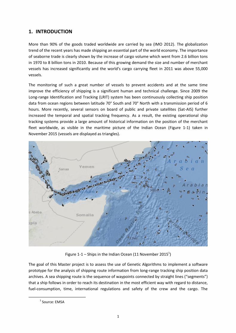
fleet worldwide, as visible in the maritime picture of the Indian Ocean (Figure 1-1) taken in
November 2015 (vessels are displayed as triangles).
Figure 1-1 – Ships in the Indian Ocean (11 November 20151)
The goal of this Master project is to assess the use of Genetic Algorithms to implement a software
prototype for the analysis of shipping route information from long-range tracking ship position data
archives. A sea shipping route is the sequence of waypoints connected by straight lines (“segments”)
that a ship follows in order to reach its destination in the most efficient way with regard to distance,
fuel-consumption, time, international regulations and safety of the crew and the cargo. The
1 Source: EMSA

2
approach proposed in this project is to analyze the tracks of many ships that sailed between two
ports (or more generally, ocean regions) in order to extract the information on the best shipping
route that connects them. The analysis of the ship tracks is done first by means of standard data
mining techniques (ETL and data reduction) and then with a Genetic Algorithm that reconstructs a
shipping route from the raw coordinates of the ship positions.
The author developed a Shipping Route Estimation software prototype, being one of the first tools
that apply Genetic Algorithms to this particular problem and with this type of dataset. The outcome
of the automatic Shipping Route Estimation has been assessed by a human expert, former
commander of oil tankers.
The results of this project may benefit the Maritime Community by increasing the efficiency of
shipping, the safety of life at sea and the protection of the environment.
1.1. MARITIME SAFETY, SHIP TRACKING, AND SHIPPING ROUTES
The project was executed in cooperation with the European Maritime Safety Agency (EMSA), based
in Lisbon. The mission of EMSA is providing services to the European Member States to prevent
accidents, protect the life of seafarers and safeguard the environment (“Quality shipping, safer seas,
cleaner Oceans”).
Knowing the location of ships at any time and at a global scale is of paramount importance to
accomplish the mission of the Agency. To this purpose EMSA provides one of the most advanced
ship tracking services in the world. The monitoring platforms for long-range ship tracking are
currently (2015) the following two systems:
LRIT: the Long-Range Identification and Tracking is a mandatory SOLAS (SOLAS, 1974)
requirement applicable to ships over 300 tons; a ship transmits its coordinates on a
secure satellite channel at a minimum fixed rate of one position report every 6 hours;
LRIT tracks ships worldwide between the latitudes 70° South and North; LRIT has been
active since July 2009.
Sat-AIS: the Satellite based Automatic Identification System is a recent tracking
technology based on the anti-collision AIS ship-to-ship communication system; the
broadcast radio signals are received by a constellation of low orbit satellites; data is
regularly downloaded to the monitoring center and the average tracking rate is
currently one position report every 4 to 5 hours; Sat-AIS data is available since 2012.
EMSA provides the long-range ship tracking data as a complement to the shore-based monitoring of
the ship traffic, which covers approximately a 50 km coastal stripe all around the EU waters. Shore-
based monitoring is performed using terrestrial AIS (T-AIS) receivers located along the coastline and
the standard tracking frequency is one position every 6 minutes. The main application of LRIT, Sat-
AIS, and T-AIS tracking is vessel traffic monitoring, where the data is made available to the user
community in real time.
3
1.2. PROJECT OBJECTIVES
The hypothesis that drives this Master project is that the historical analysis of the ship tracks and
navigational pattern between two ocean regions may lead to an automatic route estimation
algorithm. The estimated route can support the planning of the most efficient path based on the
choices made by shipmasters in the previous months or years. Applications that can benefit of long-
range tracking sources of information are the shipping route analysis and planning tools. The
decision of which route a ship should follow when sailing between two ports is an important step in
the planning and monitoring of a ship voyage.
This project aims at solving the problem of estimating the most operated shipping route between
two ocean regions by analyzing the LRIT and Sat-AIS tracking systems ship position archives
(Shipping Route Estimation problem).
The main objective of the project is the application of Genetic Algorithms to the problem of
computing the best (“fittest”) shipping route based on the positions of ships that sailed between the
departure and arrival ocean area. The chosen technical approach of this project is to develop a data
driven, non-supervised Genetic Algorithm. The operational purpose of this work is the improvement
of the route detection algorithms currently in use at EMSA and in other maritime agencies. The
Shipping Route Estimation algorithm will allow the user to base the route planning not only on
theoretical assumption on seasonal winds and currents but on the actual paths followed by
merchant ships sailing between the same two ports during the same period in the past. The project
will assess the level of confidence obtained by the algorithm through the assessment of an
experienced seafarer.
In order to achieve the main objective the following specific goals are set:
Analysis of the user’s requirements with regard to the estimation of shipping routes;
definition of the user’s needs and most relevant applications with the collaboration of
EMSA and representatives of the European Maritime Community.
Selection of the geographical areas for shipping route planning based on the user’s
needs; definition of the boundaries of the areas of interest
Selection of the data to support the analysis and algorithm tuning:
o Long-range Tracking Data (sources: LRIT, Sat-AIS)
o Periods of time for data analysis
o Relevant ship tracks between departure and arrival areas
Configuration, training and validation of the Machine Learning system based on
Genetic Algorithms
Assessment of the quality of the shipping route detection and the robustness of the
algorithm

4
1.3. RELEVANT ACTIVITIES AND PROJECTS
The European Maritime Safety Agency (EMSA) has been very active in the past 10 years in the
domain of automatic ship tracking and decision support systems for Maritime Situational Awareness.
The Agency developed the European LRIT Cooperative Data Center in 2008 which is presently hosted
and operated in Lisbon. Ship positions are collected in a fully automatic way on a 24/7 basis by
means of the Inmarsat and Iridium communication satellite networks. The data is distributed on
demand in real time to the EU Maritime Administrations, Coast Guards and Navy and other entitled
Organization worldwide.
More recently EMSA has designed and developed the IMDatE system that collects maritime traffic
data from different sources, including Sat-AIS, and provides an integrated maritime traffic picture to
the EU Maritime Community.
IMDatE implements an automatic ship behavior monitoring service that may benefit from the results
of this project. The Shipping Route Estimation algorithm in fact could be used to spot an anomalous
position pattern of a ship that is sailing between two regions outside the most operated route.
1.4. DOCUMENT STRUCTURE
This document describes the project preparation, the proposed approach based on Genetic
Algorithms, the software implementation, and the results obtained on some representative shipping
routes.
Chapter 2, Literature Review, presents a summary of the past work done on this field. The two main
topics analyzed in the scope of the projects are Shipping Route Analysis and Genetic Algorithms.
Chapter 3, Methodology, describes the approach that was taken during the project in order to
design the Shipping Route Estimation system, collect the data, prepare the data for analysis, and
implement a solution based on the available Genetic Algorithm technology. This section also outlines
the methodology that was applied to validate the results from a technical and operational
perspective.
Chapter 4, The Data, refers to the two ship tracking systems (LRIT, Sat-AIS) used in the project and
the characteristics of the ship position data available for analysis in the historical archives.
Chapter 5, Data Pre-Processing, describes the ETL process required to extract, convert and make
available the data for further analysis by the Machine Learning module. A specific section shows the
details of the Data Mart created to easily access the ship tracks.
Chapter 6, The Genetic Algorithm, illustrates in detail the algorithm and the technological solution
used in the project to implement the Machine Learning module. The chapter describes the type of
genome that represents the shipping routes to be estimated as well as the different kinds of quality
measures that define the fitness of an individual.
Chapter 7, Results, shows the outcome of the project and relates the feedback received from an
expert during the assessment of the Shipping Route Estimation system prototype. The chapter also

5
addresses the advantages and limitations of its use in a real-word application for Maritime Safety
purposes.
Chapter 8, Conclusions and Future Work, summarizes the project results and proposes possible
future developments.
6
2. LITERATURE REVIEW
This section describes the literature and previous activities that are relevant to the project work. The
papers that are directly related to the Maritime domain are analyzed with more detail. More
specifically, articles about ship tracking and route detection have been selected. A more
comprehensive reference of literature concerning Genetic Algorithms is listed in the Bibliography
(Chapter 9).
The most relevant article for the preparation of the project is the one by Pallotta G., Vespe M., and
Bryan K. (Pallotta, 2013). It presents an unsupervised and incremental learning approach to the
extraction of maritime movement patterns. The proposed methodology is called TREAD, which
stands for Traffic Route Extraction and Anomaly Detection. TREAD converts raw data, i.e. ship
position reports from different tracking platforms, into information that can be used to support
decisions concerning the safety and security of shipping. The paper shows that understanding past
maritime traffic patterns is a fundamental step towards Maritime Situational Awareness
applications, in particular, to classify and predict activities. TREAD is a basis for automatically
detecting anomalies, using past ship tracks and traffic patterns as an input to a Decision Support
System. TREAD builds a statistical model in which the traffic knowledge is extracted from the data by
means of “ship objects”, created and constantly updated based on the AIS position data stream. The
changes in the state vectors, i.e. the course and speed, of many ship objects generate a series of
spatial events that are clustered around waypoints used to reconstruct the traffic routes. Tracks that
substantially deviate from other vessel paths on the same route are considered outliers and
eliminated from the analysis. The result of the data analysis is fed into the last module of TREAD
which provides the anomaly detection and route prediction functions.
Other relevant articles about vessel traffic analysis and maritime awareness are listed here in
chronological order. Ristic (Ristic, 2008) presents a survey of vessel trajectory-based analysis for
visual surveillance. The relevant events are detected by describing the maritime scene with a
topographical model, learned by the system in an automatic way. The motion patterns are used to
construct the real-time anomaly sensors. Kazemi (Kazemi, 2013) investigates the potential of using
open data as a complementary resource to improve the data analysis techniques for anomaly
detection in maritime surveillance. Maritime open data is considered all information publicly
available on the Internet or other media and related to the maritime domain. The paper presents
and evaluates a decision support system based on open data in addition to the confidential sources
available to the Maritime Authorities. Their results indicate improvements in the efficiency and
effectiveness of the existing surveillance systems by increasing the accuracy and covering unseen
aspects of the maritime activities. In the more specific domain of fishery monitoring, Mazzarella
(Mazzarella, 2014) analyzes the AIS position data to detect and identify fishing patterns. The paper
shows that the capability of understanding events and activities within the maritime environment
can be greatly improved by the automatic identification and classification of vessel activities. The
proposed solution is applied to the practical scenario of automatically discovering fishing areas
based on historical (both terrestrial and satellite) AIS data.
The problem of reconstructing shipping lanes in a particular area is presented by Fernandez
Arguedas (Arguedas, 2014). The proposed algorithm automatically produces a network of maritime
shipping lanes extracted from historical vessel positioning data, by detecting the entry and exit

7
points in the ocean region and the so called breakpoints which divide a ship track into shorter
segments. The proposed applications are track reconstruction in cases of tracking gaps, destination
prediction, and detection of anomalous behavior.
The use of Genetic Algorithms (Goldberg, 1988) for anomaly detection in ship behavior is proposed
by Chun-Hsien Chen (Chen, 2014).They develop the knowledge discovery system GeMASS, a
machine learning software for the purpose of characterizing maritime security threats. The Genetic
Algorithm is based on a chromosome that represents a set of attributes (e.g. ship details, cargo,
inspection reports, etc.) plus the decision taken with regard to that particular individual, for instance
the risk level associated to a ship bound to a port facility. GeMASS can be used to support the
decision process of a Port Authority to assess the risk of the incoming ships (blacklisting) and
perform, if necessary, ad-hoc safety and security inspections. Genetic Algorithms have been applied
to the ship routing problem by Martins (Martins, 2010). Not to be confounded with the Shipping
Route Estimation problem, which is the topic of this project, a ship routing algorithm serves the
purpose of efficient fleet management and optimization of freight transport by sea. The different
issue of route planning for weather hazard avoidance has also been addressed by means of a
Genetic Algorithm as described by Krata (Krata, 2012). Deviating from the course due to unfavorable
weather conditions and, at the same time, meeting the navigational constraints constitute a multi-
objective optimization problem resolved with an evolutionary algorithm.
8
3. METHODOLOGY
The assessment of the application of Genetic Algorithms to the problem of Shipping Route
Estimation was done in the following phases:
1. System Design
2. Data Collection
3. Pre-processing
4. Genetic Algorithm Selection and Implementation
5. Machine Learning
6. Demonstration and Validation
3.1. THE SHIPPING ROUTE ESTIMATION SYSTEM
The initial activity of the project relates to the analysis of the requirements of a useful Shipping
Route Estimation service to be delivered to the Maritime Community. As in any technological
development, it is a good practice to check what the users’ needs are before going into the actual
design phase.
A few interviews with some representatives of the user community (seafarers, ship tracking service
providers) indicated the following main requirements:
- Estimating the most operated shipping route between two Ocean regions
- Detecting the shipping route variations by comparing the summer and winter seasonal
traffic patterns
Following this input a Data Analysis system prototype has been designed. The data is extracted from
the ship tracking historical archive, pre-processed according to the temporal and spatial criteria, and
eventually analyzed by a machine learning module. The learning process is fully data-driven, without
human supervision and based uniquely on the tracks of different ships sailing between the two
regions under analysis in the past.
The architecture of the Shipping Routes estimation system developed in this project is shown in
Figure 3.1.

9
Figure 3-1 - Shipping Route Estimation System Architecture
The three main modules of the system are:
Input Data Processing: the module is responsible for the pre-processing and loading of
the input data into the database (Chapter 5.1).
Database: the module stores, filters and make the ship positions accessible for further
analysis by means of the Shipping Route Data Mart (Chapter 5.2).
Machine Learning Module: a suite of software components that analyze the data and
extract the relevant knowledge using Genetic Algorithms (Chapter 6).
3.2. DATA COLLECTION
The dataset used in the scope of the project was retrieved from the LRIT ship position archive at
EMSA and from the Sat-AIS ship position archives of the data providers. In order to have access to
the data for the purpose of this study, a request for authorization was approved by the following
Organizations:
- Sat-AIS data
o The Norwegian Coastal Administration “Kystverket” 2
o The Company “exactEarth” 3
2 Institutional website: http://www.kystverket.no
3 Company website: http://www.exactearth.com

10
- LRIT data
o The Maltese Merchant Shipping Directorate “Transport Malta”4
o The Italian Authority “Guarda Costiera Italiana”5
All involved parties authorized the use of the data for the purpose of the execution of this project6.
The total number of positions records collected and analyzed in the scope of the project is over 370
million from more than 100,000 ships.
A summary of the input data volume by tracking system is shown in Table 3.1. The reference period
is from January 2011 to December 2012 (2 years).
Tracking System
# Ships Total # Position Reports
(millions)
LRIT7 2,600 6.6
Sat-AIS 101,000 365
Table 3.1 – Input Data Volume by Tracking System
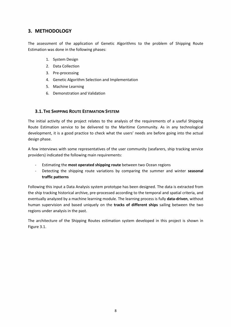
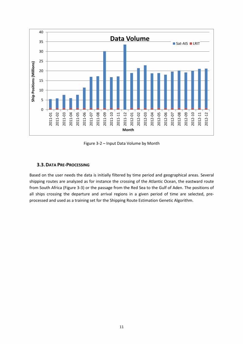
The chart in Figure 3.2 shows the volume of ship positions per month during the reference period. It
is visible the difference in volume of the LRIT data and the Sat-AIS data. This is due to the smaller
number of LRIT ships considered by this project compared to the much larger fleet of vessels tracked
by Sat-AIS.
4 Institutional website: http://www.transport.gov.mt
5 Institutional website: http://www.guardiacostiera.gov.it
6 As agreed with the data providers, the ship positions have been fully anonymized and the project
results are published in an aggregate form, without any reference to the identification, the flag or any other sensitive ship details. The data or any derived product developed in the scope of this project will not be used for commercial applications. At the end of the project the dataset used for the analysis has been destroyed.
7 The LRIT figures refer to the fleet of Malta (approx. 2000 ships) and Italy (approx. 600 ships).
11
Figure 3-2 – Input Data Volume by Month
3.3. DATA PRE-PROCESSING
Based on the user needs the data is initially filtered by time period and geographical areas. Several
shipping routes are analyzed as for instance the crossing of the Atlantic Ocean, the eastward route
from South Africa (Figure 3-3) or the passage from the Red Sea to the Gulf of Aden. The positions of
all ships crossing the departure and arrival regions in a given period of time are selected, pre-
processed and used as a training set for the Shipping Route Estimation Genetic Algorithm.
0
5
10
15
20
25
30
35
40
20
11
-01
20
11
-02
20
11
-03
20
11
-04
20
11
-05
20
11
-06
20
11
-07
20
11
-08
20
11
-09
20
11
-10
20
11
-11
20
11
-12
20
12
-01
20
12
-02
20
12
-03
20
12
-04
20
12
-05
20
12
-06
20
12
-07
20
12
-08
20
12
-09
20
12
-10
20
12
-11
20
12
-12
Ship
Po
siti
on
s (M
illio
ns)
Month
Data Volume Sat-AIS LRIT

12
Figure 3-3 – Sample Ship Tracks between Capetown (green box) and Réunion (orange box)
The data cleansing during the pre-processing phase is based on data quality checks with respect to:
Data Relevance: ship sailing between the two regions under analysis on an
abnormally long route are considered outliers and are eliminated
Data Completeness: ships with very few positions between the two regions under
analysis do not contribute in a significant way to the input data and are eliminated
Data Redundancy: multiple positions received in a very short time interval from the
same ship are considered redundant and are eliminated
After data cleansing, the last step of the pre-processing phase aims the time normalization of the
ship positions based on the assumption of constant voyage duration: all ships start at the same time
and reach the destination after the same fixed period of time (in the actual implementation the
voyage duration equals 24 hours). Further details on the data pre-processing procedure are
described in Chapter 5.
3.4. ALGORITHM SELECTION AND IMPLEMENTATION
Once the data selection and pre-processing tasks are completed, an analysis of the use case
scenarios is performed in order to define the detailed requirements of the machine learning system
to be developed. The most appropriate Genetic Algorithms is chosen, prototyped and tested on a
sample subset of the data: positions from a limited geographical area and from a few well known
ships.
The actual Genetic Algorithm implementation is based on the open source library ECJ (Luke 2014),
developed at George Mason University's ECLab Evolutionary Computation Laboratory8. The ECJ basic
8 Laboratory website: https://cs.gmu.edu/~eclab
13
species prototypes are enhanced and adapted to the specific problem of Shipping Route Estimation.
The chosen representation of a solution is an individual belonging to a Vector species. The species is
characterized by a gene composed of a sequence of decimal numbers that represent displacements
on a 2-dimensional space. An individual of such a species is evaluated by reconstructing the
corresponding track and computing its fitness to solve the Shipping Route Estimation problem.
3.5. MACHINE LEARNING ALGORITHM
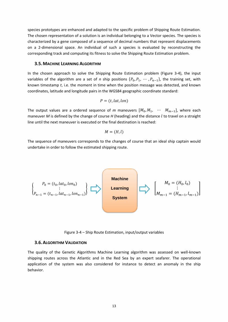
In the chosen approach to solve the Shipping Route Estimation problem (Figure 3-4), the input
variables of the algorithm are a set of n ship positions {𝑃0, 𝑃1, ⋯ , 𝑃𝑛−1}, the training set, with
known timestamp t, i.e. the moment in time when the position message was detected, and known
coordinates, latitude and longitude pairs in the WGS84 geographic coordinate standard:
𝑃 = (𝑡, 𝑙𝑎𝑡, 𝑙𝑜𝑛)
The output values are a ordered sequence of m maneuvers [𝑀0,𝑀1, ⋯ 𝑀𝑚−1], where each
maneuver M is defined by the change of course H (heading) and the distance 𝑙 to travel on a straight
line until the next maneuver is executed or the final destination is reached:
𝑀 = (𝐻, 𝑙)
The sequence of maneuvers corresponds to the changes of course that an ideal ship captain would
undertake in order to follow the estimated shipping route.
Figure 3-4 – Ship Route Estimation, input/output variables
3.6. ALGORITHM VALIDATION
The quality of the Genetic Algorithms Machine Learning algorithm was assessed on well-known
shipping routes across the Atlantic and in the Red Sea by an expert seafarer. The operational
application of the system was also considered for instance to detect an anomaly in the ship
behavior.
Machine
Learning
System
𝑃0 = (𝑡0, 𝑙𝑎𝑡0, 𝑙𝑜𝑛0)
⋮𝑃𝑛−1 = (𝑡𝑛−1, 𝑙𝑎𝑡𝑛−1, 𝑙𝑜𝑛𝑛−1)
𝑀0 = (𝐻0, 𝑙0)
⋮𝑀𝑚−1 = (𝐻𝑚−1, 𝑙𝑚−1)

14
4. THE DATA
The basis of this project was the large data archive of ship positions collected in the past years from
the LRIT and Sat-AIS tracking systems.
4.1. LONG-RANGE IDENTIFICATION AND TRACKING (LRIT)
The Long-Range Identification and Tracking system (LRIT) started operations in July 2009 and it is an
initiative of the International Maritime Organization (IMO), the United Nations body responsible for
the maritime safety. LRIT is composed of a device on board the ship that sends a message with ship
identification and its GPS position through a satellite link with a regular period of 6 hours. For over
95% of the ships, the LRIT message is received by one of the INMARSAT geostationary satellites and
retransmitted to a land station. In some cases, particularly for ships that sail in the Polar regions,
other telecommunication low-orbit satellite networks are used, as for instance Iridium. The LRIT
position data is eventually stored and made available to the maritime community by one of the LRIT
data centers. EMSA operates the LRIT Data Center of the European Union which tracks over 9000
ships worldwide.
4.1.1. Characteristics of the LRIT Data
According to the IMO resolution9 and amendment of SOLAS (IMO 1974), LRIT is a mandatory tracking
system for any ship operating on an international route and with a weight over the 300 gross tons.
This corresponds to approximately 9000 ships in the case of the fleets flying the flag of one of the EU
Member States.
The main objective of the LRIT system is a worldwide continuous, regular and secure 6-hour tracking
of the ship.
In practice, since the INMARSAT satellite telecommunication network is available in the ocean
regions between latitude 70° South and 70° North, this is also the actual coverage of the LRIT
tracking service. Even if the ships sailing in the Arctic and Antarctic regions are not “seen” by LRIT via
INMARSAT, the service is well fit to follow the main world shipping routes and collect a constant flow
of data from a large number of merchant vessels sailing from all the major ports.
Although the LRIT on-board equipment can transmit the position information with a rate of up to
one message every 15 minutes, the standard 6-hour period, i.e. 4 messages per day, is the
transmission rate used by the overwhelming majority of the ships. This may be considered a
limitation of the tracking quality of the LRIT service given that a ship with a typical speed of 20 knots
(approx. 37 km/h) covers a distance of over 200 km in 6 hours and during this time interval there is
no information available about the whereabouts of the ship.
For the purpose of this project however the LRIT data is a valuable source of information thanks to
the fact that we can combine the tracks of several ships sailing between the same regions and
therefore partially filling the gaps in the track of a single vessel.
9 MSC.202(81), 2006

15
Another complementary tracking system that can provide further detail to the maritime picture is
Sat-AIS which is described in the following section.
4.2. SAT-AIS
The Automatic Identification System (AIS) was originally developed as a ship-to-ship broadcast
transmission device for collision avoidance at sea. AIS sends over VHF several messages that provide
information on the ship identification, speed, heading, destination, etc. The most important
messages in the scope of this project are the AIS Message Types 1, 2, and 3 that contain the
coordinates of the ship location at the time of transmission.
The transmission rate of AIS is much higher than LRIT and the typical configuration of the AIS
tracking system is one message every 6 minutes. The range of the AIS signal however is limited by
the line-of-sight distance to the receiving antenna and shore based AIS receiving stations manage to
track ships up to 100 km from the coast, depending on the position of the antenna and weather
conditions.
In recent years thanks to the progress in space technology, AIS receiving devices have been installed
on board of low orbiting satellites and the International Space Station. The new tracking platform is
called Satellite-AIS (Sat-AIS). The result of this technological development is that the AIS messages
from ships can now be acquired worldwide even if they are sailing far from the coastline.
4.2.1. Characteristics of the Sat-AIS Data
Similarly to LRIT, the tracking rate of Sat-AIS is still relatively low. Based on the orbit of the satellites,
the detection is not regular: many position messages from the same ship can be received in a period
of few minutes followed by a detection gap of 5 or 6 hours. This situation will improve in the coming
years thanks to the launch of more and more satellites equipped with AIS sensors.
Compared to LRIT, the amount of Sat-AIS data is much larger in spite of a less regular data stream,
with highly variable tracking frequency and timeliness depending on the orbit of the satellites and
the location of the receiving stations on the ground. In addition to the location of the ship, Sat-AIS
messages also contain the values of the course and speed of the ship.
16
5. DATA PRE-PROCESSING
In order to compute the most operated route between two ports we extract the input data from the
historical ship position archive of LRIT and Sat-AIS data by executing the following steps:
AIS Pre-Processing chain
o Extraction and Decoding of AIS position messages
o Loading of AIS positions into the Staging Area
o AIS Data Reduction (removal of duplicates) and Integrity Check
o Selection of AIS position
LRIT Pre-Processing chain
o Loading of LRIT positions into the Staging Area
o Integrity Check
o Selection of LRIT position
5.1. EXTRACT, TRANSFORM AND LOAD (ETL)
The message broadcast by the AIS equipment on board a ship can be of 27 different types. Some
messages contain static information about the ship, for instance its name and identification codes or
the type of vessel. Other messages, which are the most interesting in the scope of this project,
communicate the current position of the ship, in latitude and longitude coordinates provided by the
GPS on-board receiver.
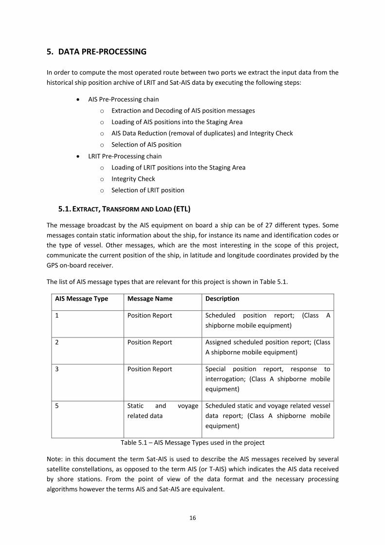
The list of AIS message types that are relevant for this project is shown in Table 5.1.
AIS Message Type Message Name Description
1 Position Report Scheduled position report; (Class A
shipborne mobile equipment)
2 Position Report Assigned scheduled position report; (Class
A shipborne mobile equipment)
3 Position Report Special position report, response to
interrogation; (Class A shipborne mobile
equipment)
5 Static and voyage
related data
Scheduled static and voyage related vessel
data report; (Class A shipborne mobile
equipment)
Table 5.1 – AIS Message Types used in the project
Note: in this document the term Sat-AIS is used to describe the AIS messages received by several
satellite constellations, as opposed to the term AIS (or T-AIS) which indicates the AIS data received
by shore stations. From the point of view of the data format and the necessary processing
algorithms however the terms AIS and Sat-AIS are equivalent.

17
The overall AIS data processing chain is described in the diagram of Figure 5-1.
Figure 5-1 – Sat-AIS data processing chain
The two main processing steps are:
AIS Message Decoding: conversion from the native binary (raw) data format into plain
text Comma Separated Value (CSV)
Load into Staging Area: load of the position messages into a Staging Area database
5.1.1. AIS Message Datasets
The first dataset analyzed during the pre-processing phase of the project was the Sat-AIS data
archive kindly provided by the Norwegian Coastal Administration “Kystverket”.
The input data is stored in plain ASCII text files in which each line contains an AIS encoded in NMEA
format. This standard message format was defined by the National Marine Electronics Association
and it is used for binary communication between marine equipment. See an excerpt of an NMEA AIS
data stream in Annex 10.1.
In order to decode the AIS data stream and extract the identification and position information from
the messages, a Java application was implemented based on the publicly available library DMA
AisLib made available by the Danish Maritime Authority10.
The second Sat-AIS dataset kindly provided by the Company exactEarth was already decoded and
available in CSV format for further processing.
5.1.2. Load into Staging Area
Once the relevant data items were extracted and converted into a readable format (CSV), the AIS
position reports were loaded into the Staging Area of the data analysis system.
At this point of the processing chain, the step “Load into Staging Area” is applicable both to AIS and
LRIT data. In fact the LRIT position reports, similarly to the exactEarth dataset, are already available
in CSV format. The LRIT dataset was kindly provided by the Maritime Authorities of Italy, the
“Guardia Costiera Italiana”, and Malta, “Transport Malta”.
The Staging Area is an intermediate archive that temporarily stores the input data before further
processing. During the project the Staging Area was mainly used to load data from a given data
10
Code repository: https://github.com/dma-ais/AisLib
18
provider, in the case of Sat-AIS from Norway and exactEarth, and for a given period of time (several
months or a full year), based on the input data files.
The use of a Staging Area in this project was justified by the extremely large amount of data to be
analyzed. Developing the first prototypes to visualize and analyze the ship positions was much easier
by taking as an input the position report from a short period of time. Dropping and recreating the
Staging Area was relatively simple. Moreover the data loading process was faster, considering the
time needed to create the database indexes necessary for the following processing steps.
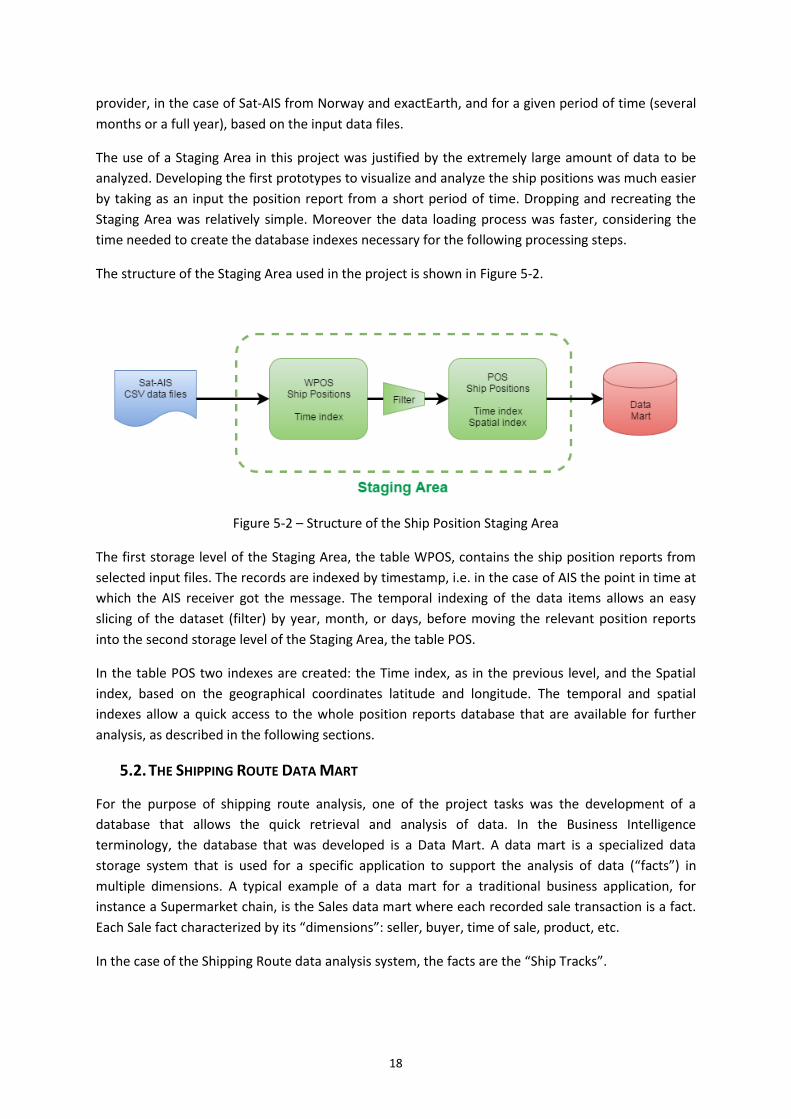
The structure of the Staging Area used in the project is shown in Figure 5-2.
Figure 5-2 – Structure of the Ship Position Staging Area
The first storage level of the Staging Area, the table WPOS, contains the ship position reports from
selected input files. The records are indexed by timestamp, i.e. in the case of AIS the point in time at
which the AIS receiver got the message. The temporal indexing of the data items allows an easy
slicing of the dataset (filter) by year, month, or days, before moving the relevant position reports
into the second storage level of the Staging Area, the table POS.
In the table POS two indexes are created: the Time index, as in the previous level, and the Spatial
index, based on the geographical coordinates latitude and longitude. The temporal and spatial
indexes allow a quick access to the whole position reports database that are available for further
analysis, as described in the following sections.
5.2. THE SHIPPING ROUTE DATA MART
For the purpose of shipping route analysis, one of the project tasks was the development of a
database that allows the quick retrieval and analysis of data. In the Business Intelligence
terminology, the database that was developed is a Data Mart. A data mart is a specialized data
storage system that is used for a specific application to support the analysis of data (“facts”) in
multiple dimensions. A typical example of a data mart for a traditional business application, for
instance a Supermarket chain, is the Sales data mart where each recorded sale transaction is a fact.
Each Sale fact characterized by its “dimensions”: seller, buyer, time of sale, product, etc.
In the case of the Shipping Route data analysis system, the facts are the “Ship Tracks”.

19
5.2.1. Ship Tracks
Once the relevant ship positions are extracted from the staging area, a particular database is
populated: the “Ship Tracks” data mart. A Ship Track is an ordered sequence of ship positions. If the
positions are connected with straight lines, the result is a series of segments forming a path that
connects two ocean regions. A ship track is also called a Ship Voyage when the track is the collection
of real positions detected by a tracking system in a certain period of time and referring to the same
ship, actually sailing between the departure and arrival areas under analysis.
The data mart thus contains a fact table of Ship Tracks that can be sliced along the following
dimensions:
Time (period of the year)
Ship Type
Area of Departure
Area of Arrival
The data mart is populated by means of a data mining tool (see Annex 10.4).
In order to better understand the different dimensions of the data mart and its loading process,
Figure 5-3 shows some sample ship tracks between the Canary Islands and Brazil.
20
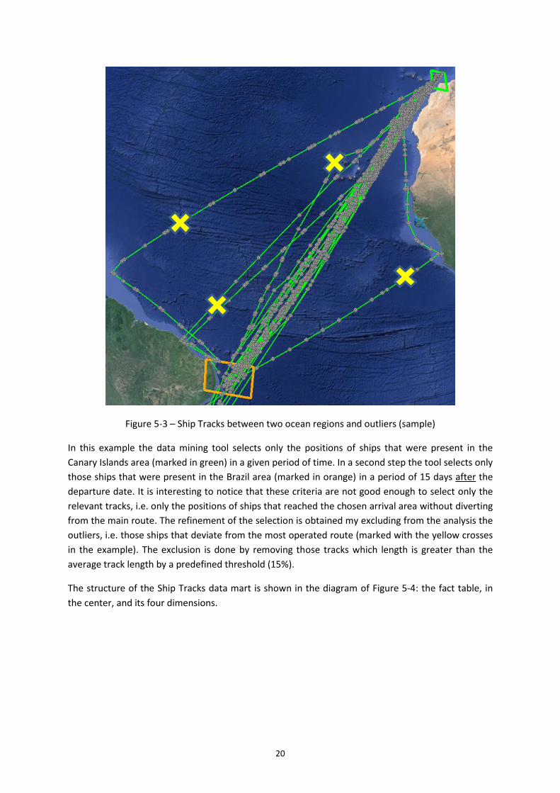
Figure 5-3 – Ship Tracks between two ocean regions and outliers (sample)
In this example the data mining tool selects only the positions of ships that were present in the
Canary Islands area (marked in green) in a given period of time. In a second step the tool selects only
those ships that were present in the Brazil area (marked in orange) in a period of 15 days after the
departure date. It is interesting to notice that these criteria are not good enough to select only the
relevant tracks, i.e. only the positions of ships that reached the chosen arrival area without diverting
from the main route. The refinement of the selection is obtained my excluding from the analysis the
outliers, i.e. those ships that deviate from the most operated route (marked with the yellow crosses
in the example). The exclusion is done by removing those tracks which length is greater than the
average track length by a predefined threshold (15%).
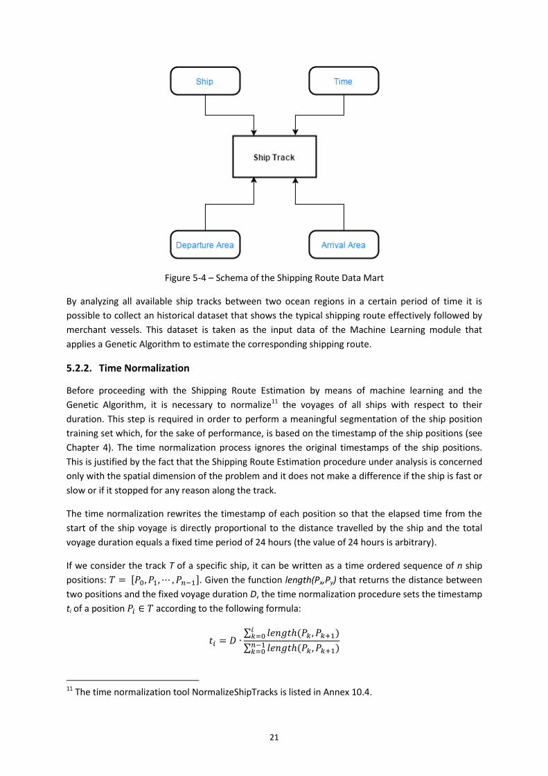
The structure of the Ship Tracks data mart is shown in the diagram of Figure 5-4: the fact table, in
the center, and its four dimensions.
21
Figure 5-4 – Schema of the Shipping Route Data Mart
By analyzing all available ship tracks between two ocean regions in a certain period of time it is
possible to collect an historical dataset that shows the typical shipping route effectively followed by
merchant vessels. This dataset is taken as the input data of the Machine Learning module that
applies a Genetic Algorithm to estimate the corresponding shipping route.
5.2.2. Time Normalization
Before proceeding with the Shipping Route Estimation by means of machine learning and the
Genetic Algorithm, it is necessary to normalize11 the voyages of all ships with respect to their
duration. This step is required in order to perform a meaningful segmentation of the ship position
training set which, for the sake of performance, is based on the timestamp of the ship positions (see
Chapter 4). The time normalization process ignores the original timestamps of the ship positions.
This is justified by the fact that the Shipping Route Estimation procedure under analysis is concerned
only with the spatial dimension of the problem and it does not make a difference if the ship is fast or
slow or if it stopped for any reason along the track.
The time normalization rewrites the timestamp of each position so that the elapsed time from the
start of the ship voyage is directly proportional to the distance travelled by the ship and the total
voyage duration equals a fixed time period of 24 hours (the value of 24 hours is arbitrary).
If we consider the track T of a specific ship, it can be written as a time ordered sequence of n ship
positions: 𝑇 = [𝑃0, 𝑃1, ⋯ , 𝑃𝑛−1]. Given the function length(Px,Py) that returns the distance between
two positions and the fixed voyage duration D, the time normalization procedure sets the timestamp
ti of a position 𝑃𝑖 ∈ 𝑇 according to the following formula:
𝑡𝑖 = 𝐷 ∙∑ 𝑙𝑒𝑛𝑔𝑡ℎ(𝑃𝑘 , 𝑃𝑘+1)
𝑖𝑘=0
∑ 𝑙𝑒𝑛𝑔𝑡ℎ(𝑃𝑘 , 𝑃𝑘+1)𝑛−1𝑘=0
11 The time normalization tool NormalizeShipTracks is listed in Annex 10.4.

22
6. THE GENETIC ALGORITHM
The proposed approach to extract the shipping route information from the ship position dataset is
based on a Genetic Algorithm. This chapter presents the concept of Genetic Algorithms and how this
technique is applied to the specific problem of Shipping Route Estimation.
6.1. DESCRIPTION OF GENETIC ALGORITHMS
A Genetic Algorithm (Goldberg 1988) is an artificial process that
imitates the natural phenomena of selection, breeding, mutation and
evolution of a species according to the Darwinian Theory. Such an
algorithm can be described as a heuristic, i.e. a method that solves an
optimization problem in a limited period of time by finding a solution
that, although possibly not optimal, meets the requirements of the
users.
The problem to be addressed by a Genetic Algorithm can be
represented as a challenge that some individual belonging to a
particular species has to face and overcome. The capacity of this
individual to complete the challenge with a high score and therefore
to solve the problem is quantitatively measured by means of the
individual’s “fitness”. Finding the individual with the best fitness,
given the limited time and resources at disposal, is the goal of the
Genetic Algorithm. At the end of the execution of the algorithm the
best individual can be considered the “solution” to the problem.
All individuals belong to the same species and have some basic
characteristics in common. These characteristics are expressed by
defining the structure of the genome and its genes based on the type
of solution we are aiming at.
A Genetic Algorithm starts its task on a population of randomly
generated individuals, as shown in Figure 6-1. The next step is the
evaluation of the fitness of each individual as a possible solution to
the problem. Based on the result of the fitness evaluation, the
Selection step retrieves from the population some individuals that
are going to be used as the parents of the next generation. Several
Selection strategies can be implemented, for instance fitness
proportionate or tournament. A particular type of selection is the so
called “elitism” in which the best individuals of each generation are
kept unchanged in the next one.
After selection, the group of chosen individuals is divided in pairs and the Crossover operation is
applied. Similarly to what happens in Nature, the chromosomes of the parents are mixed to breed
an offspring that inherits some characteristics of both. As in the case of Selection, different
Crossover techniques can be applied given the structure of the genome. Examples are one-point and
Figure 6-1 – Flow chart of a Genetic Algorithm
23
two-point crossover where sequences of the parent chromosomes are picked by cutting them in one
or two points and subsequently swapped to generate the children.
The final step of the process is the so called Mutation which is again inspired from Nature. Mutation
introduces, with a relatively low probability, some random changes in the genes of the offspring. In
the whole procedure, mutation is an important step that helps finding “original” individuals that
slightly diverge from the mass and can eventually lead to a better solution.
The entire breeding process is then repeated many times. At each run a new generation of
individuals is born until one of the following criteria is met:
An ideal solution was found
The maximum predefined number of generations is reached
The result of the execution of the Genetic Algorithm is an individual that evolves from a random
population of unskilled “folks” and becomes a champion that, hopefully, will solve the challenge
posed by the problem.
The next sections show how the Shipping Route Estimation problem was modelled in order to apply
a develop and apply a Genetic Algorithm to the input ship position training dataset.
6.2. SHIPPING ROUTE MODELLING
A shipping route between two ports (port of arrival and port of departure) can be modelled as a
sequence of connected segments. The first end point of the first segment is located within the
region of the port of departure. The second end point of the last segment is located within the
region of the port of arrival. The point connecting the route segments are called “waypoints” and
correspond to a change of course of the ship.
The problem of estimation and reconstruction of a shipping route therefore can be seen as the
search for a sequence of segments (displacements) in the 2-dimensional space of the ocean surface.
A waypoint on this surface is identified by a pair of geographical coordinates12, latitude and
longitude:
(𝑙𝑎𝑡, 𝑙𝑜𝑛) ∈ ℝ × ℝ
A route segment from the waypoint A with coordinates (𝑙𝑎𝑡𝐴, 𝑙𝑜𝑛𝐴) to the waypoint B with
coordinates (𝑙𝑎𝑡𝐵, 𝑙𝑜𝑛𝐵), corresponds to a displacement vector 𝑑 = (∆𝑙𝑎𝑡, ∆𝑙𝑜𝑛) where:
∆𝑙𝑎𝑡 = 𝑙𝑎𝑡𝐵 − 𝑙𝑎𝑡𝐴
∆𝑙𝑜𝑛 = 𝑙𝑜𝑛𝐵 − 𝑙𝑜𝑛𝐴
An example is shown is Figure 6-2.
12
For sake of simplicity the model does not consider the geographic boundaries of the Earth spherical surface.
24
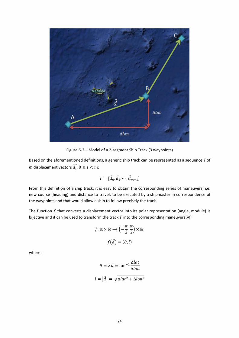
Figure 6-2 – Model of a 2-segment Ship Track (3 waypoints)
Based on the aforementioned definitions, a generic ship track can be represented as a sequence T of
m displacement vectors 𝑑𝑖⃗⃗⃗⃗ , 0 ≤ 𝑖 < 𝑚:
𝑇 = [𝑑0, 𝑑1,⋯ , 𝑑𝑚−1]
From this definition of a ship track, it is easy to obtain the corresponding series of maneuvers, i.e.
new course (heading) and distance to travel, to be executed by a shipmaster in correspondence of
the waypoints and that would allow a ship to follow precisely the track.
The function 𝑓 that converts a displacement vector into its polar representation (angle, module) is
bijective and it can be used to transform the track 𝑇 into the corresponding maneuvers ℳ:
𝑓:ℝ × ℝ ⟶ (−𝜋
2,𝜋
2) × ℝ
𝑓(𝑑) = (𝜃, 𝑙)
where:
𝜃 = ∠𝑑 = tan−1∆𝑙𝑎𝑡
∆𝑙𝑜𝑛
𝑙 = |𝑑| = √∆𝑙𝑎𝑡2 + ∆𝑙𝑜𝑛2

25
The distance 𝑙 to be travelled by the ship is the module of the displacement vector13 and the new
course 𝐻, which is always relative to the geographic North, is derived from the angle 𝜃.
The modelling approach presented above provides the appropriate “language” to represent the
Shipping Route Estimation problem in the following terms:
To be noted is the fact that since the relationship 𝑓 between a track and the resulting sequence of
maneuvers is a one-to-one correspondence, as explained above, finding the best sequence of
maneuvers is equivalent to finding the track from which it is derived.
The implementation of the model and the proposed fitness criteria are presented in the next
sections.
6.3. REPRESENTATION OF A SHIP TRACK
In a Genetic Algorithm the most adequate representation of a ship track, i.e. the solution for the
Shipping Route Estimation problem, is a species of individuals with a genome of bi-variate genes and
variable length.
A gene is a displacement vector, i.e. a pair of floating point numbers that represent the change of
latitude (∆𝑙𝑎𝑡) and longitude (∆𝑙𝑜𝑛) from one waypoint of the track to the next. If the ∆𝑙𝑎𝑡 value is
positive the displacement is towards North, if it is negative towards South. In a similar way,
∆𝑙𝑜𝑛 > 0 means a change in coordinates towards East, ∆𝑙𝑜𝑛 < 0 towards West. The magnitude of
change of each displacement vector is limited to a maximum, which is the same value both in
latitude and longitude direction.
The length of the genome is not fixed a priori but it can vary from a minimum 𝐿𝑚𝑖𝑛 to a maximum
𝐿𝑚𝑎𝑥 number of genes, giving the algorithm the freedom to find the most appropriate genome size
resulting in a balanced number of waypoints of the resulting track.
13
The shortest distance between two points on the Earth surface is approximated with the Cartesian distance.
ℳ = [𝑀0,𝑀1,⋯ ,𝑀𝑚−1]
℘ = {𝑃0, 𝑃1,⋯ , 𝑃𝑛−1}
Shipping Route Estimation problem
Find the list of 𝑚 waypoints corresponding to the
sequence of maneuvers ℳ:
that best matches the fitness criteria applied to the
training set ℘ of n positions:
of ships sailing between two ocean regions.
26
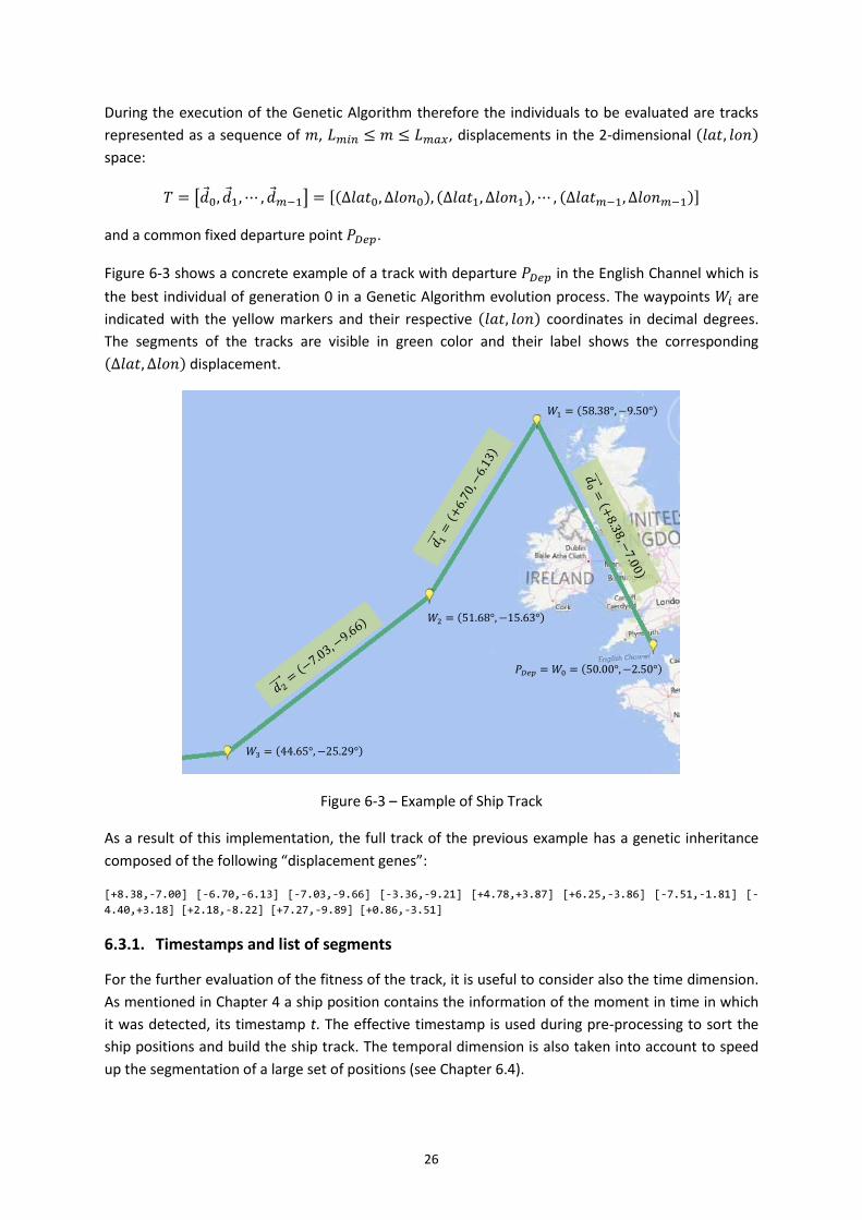
During the execution of the Genetic Algorithm therefore the individuals to be evaluated are tracks
represented as a sequence of 𝑚, 𝐿𝑚𝑖𝑛 ≤ 𝑚 ≤ 𝐿𝑚𝑎𝑥, displacements in the 2-dimensional (𝑙𝑎𝑡, 𝑙𝑜𝑛)
space:
𝑇 = [𝑑0, 𝑑1, ⋯ , 𝑑𝑚−1] = [(∆𝑙𝑎𝑡0, ∆𝑙𝑜𝑛0), (∆𝑙𝑎𝑡1, ∆𝑙𝑜𝑛1),⋯ , (∆𝑙𝑎𝑡𝑚−1, ∆𝑙𝑜𝑛𝑚−1)]
and a common fixed departure point 𝑃𝐷𝑒𝑝.
Figure 6-3 shows a concrete example of a track with departure 𝑃𝐷𝑒𝑝 in the English Channel which is
the best individual of generation 0 in a Genetic Algorithm evolution process. The waypoints 𝑊𝑖 are
indicated with the yellow markers and their respective (𝑙𝑎𝑡, 𝑙𝑜𝑛) coordinates in decimal degrees.
The segments of the tracks are visible in green color and their label shows the corresponding
(∆𝑙𝑎𝑡, ∆𝑙𝑜𝑛) displacement.
Figure 6-3 – Example of Ship Track
As a result of this implementation, the full track of the previous example has a genetic inheritance
composed of the following “displacement genes”:
[+8.38,-7.00] [-6.70,-6.13] [-7.03,-9.66] [-3.36,-9.21] [+4.78,+3.87] [+6.25,-3.86] [-7.51,-1.81] [-
4.40,+3.18] [+2.18,-8.22] [+7.27,-9.89] [+0.86,-3.51]
6.3.1. Timestamps and list of segments
For the further evaluation of the fitness of the track, it is useful to consider also the time dimension.
As mentioned in Chapter 4 a ship position contains the information of the moment in time in which
it was detected, its timestamp t. The effective timestamp is used during pre-processing to sort the
ship positions and build the ship track. The temporal dimension is also taken into account to speed
up the segmentation of a large set of positions (see Chapter 6.4).
𝑃𝐷𝑒𝑝 = 𝑊0 = (50.00°,−2.50°)
𝑊1 = (58.38°,−9.50°)
𝑊2 = (51.68°,−15.63°)
𝑊3 = (44.65°,−25.29°)

27
A practical way of representing a ship track and the timestamp of her position in correspondence to
the waypoints is a sequence of segments. A segment S of the straight line connecting two ship
positions 𝑃1 and 𝑃2 is expressed by:
𝑆 = (𝑃1, 𝑃2)
and the time interval ∆𝑡𝑆 elapsed during a voyage along the segment is given by:
∆𝑡𝑆 = 𝑡2 − 𝑡1
If a ship is located at the departure point 𝑃𝐷𝑒𝑝 at 𝑡 = 𝑡0 and performs the series of displacements
defined in a track, the resulting path, also known as a “voyage”, can be expressed as a list of
segments 𝑆𝑖 connecting the waypoints [𝑊0,𝑊1,⋯ ,𝑊𝑚]:
𝑆𝑖 = (𝑊𝑖 ,𝑊𝑖+1)
where 𝑊𝑖 = (𝑡𝑖, 𝑙𝑎𝑡𝑖 , 𝑙𝑜𝑛𝑖) and 𝑊0 = 𝑃𝐷𝑒𝑝.
According to this notation, the voyage is defined as:
𝑉 = [𝑆0, 𝑆1,⋯ , 𝑆𝑚−1]
It is straightforward to compute the total duration ∆𝑡𝑉 of the voyage:
∆𝑡𝑉 = 𝑡𝑚 − 𝑡0
and its total length 𝐿𝑉:
𝐿𝑉 = ∑ 𝑙𝑒𝑛𝑔𝑡ℎ(𝑆𝑖)
𝑚−1
𝑖=0
where 𝑙𝑒𝑛𝑔𝑡ℎ(𝑆) is the length of the segment S, given by the Cartesian distance of its two end
points with coordinates in the (lat, lon) plane. In this particular case:
𝑙𝑒𝑛𝑔𝑡ℎ(𝑆𝑖) = 𝑙𝑒𝑛𝑔𝑡ℎ(𝑊𝑖,𝑊𝑖+1) = |𝑑𝑖⃗⃗⃗⃗ |
It is evident that if the time information of a voyage is ignored, the voyage V can be used as
synonymous of its underlying track T and vice versa.
6.3.2. Crossover and Mutation of Tracks
This section describes how the Crossover and Mutation operators used by the Genetic Algorithm
influence the breeding of a new generation of individuals (tracks),modelled as a sequence of
displacements or segments.
First of all it is important to notice that both operators crossover and mutation are not always
applied after the selection step. The probability parameters of using (or not) the operators are set in
the ECJ configuration file (see Section 6.6.1). The probability (or likelihood) is expressed as usual with
a value in the interval [0,1], where 0 means that the operator is never applied, while 1 means that
the operator is applied at any breeding cycle.
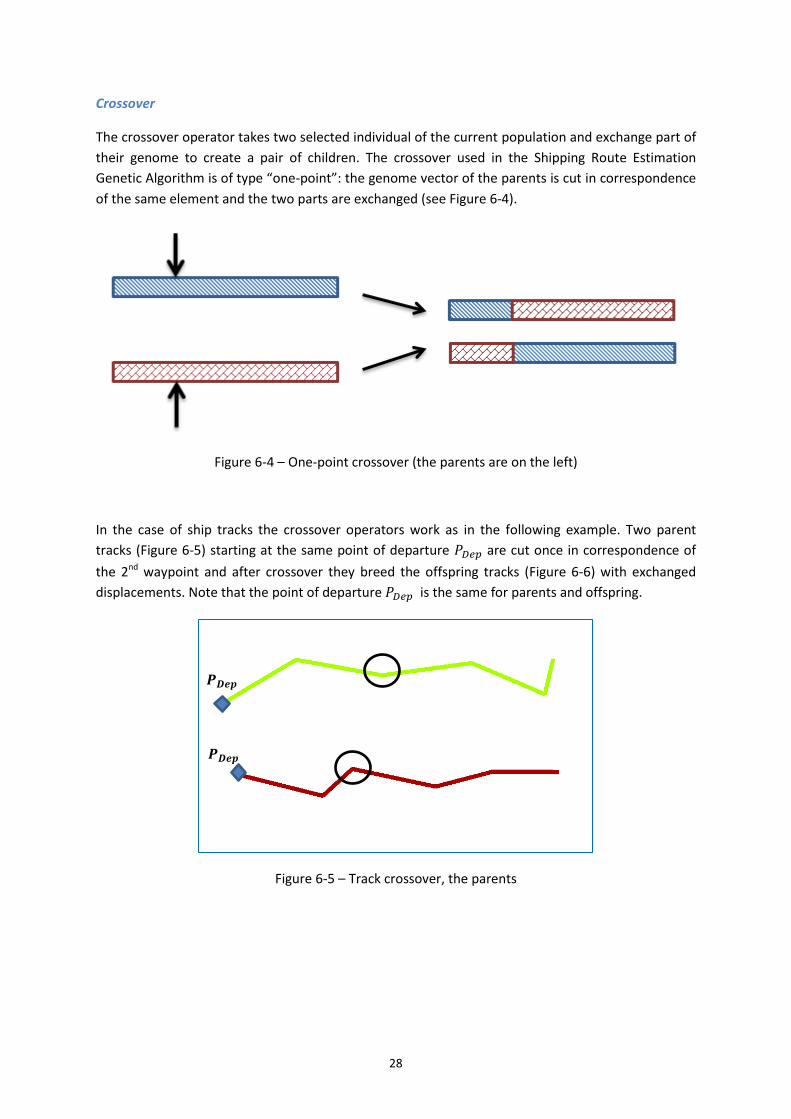
28
Crossover
The crossover operator takes two selected individual of the current population and exchange part of
their genome to create a pair of children. The crossover used in the Shipping Route Estimation
Genetic Algorithm is of type “one-point”: the genome vector of the parents is cut in correspondence
of the same element and the two parts are exchanged (see Figure 6-4).
Figure 6-4 – One-point crossover (the parents are on the left)
In the case of ship tracks the crossover operators work as in the following example. Two parent
tracks (Figure 6-5) starting at the same point of departure 𝑃𝐷𝑒𝑝 are cut once in correspondence of
the 2nd waypoint and after crossover they breed the offspring tracks (Figure 6-6) with exchanged
displacements. Note that the point of departure 𝑃𝐷𝑒𝑝 is the same for parents and offspring.
Figure 6-5 – Track crossover, the parents
𝑷𝑫𝒆𝒑
𝑷𝑫𝒆𝒑
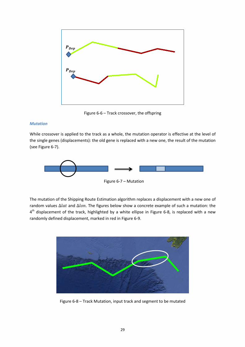
29
Figure 6-6 – Track crossover, the offspring
Mutation
While crossover is applied to the track as a whole, the mutation operator is effective at the level of
the single genes (displacements): the old gene is replaced with a new one, the result of the mutation
(see Figure 6-7).
The mutation of the Shipping Route Estimation algorithm replaces a displacement with a new one of
random values ∆𝑙𝑎𝑡 and ∆𝑙𝑜𝑛. The figures below show a concrete example of such a mutation: the
4th displacement of the track, highlighted by a white ellipse in Figure 6-8, is replaced with a new
randomly defined displacement, marked in red in Figure 6-9.
Figure 6-8 – Track Mutation, input track and segment to be mutated
Figure 6-7 – Mutation
𝑷𝑫𝒆𝒑
𝑷𝑫𝒆𝒑

30
Figure 6-9 – Track Mutation, output track with the mutated segment marked in red
6.4. THE SEARCH FOR FITNESS
One of the most important steps in the execution of a Genetic Algorithm is the evaluation of the
fitness of an individual. In the Shipping Route Estimation problem the fitness of a candidate shipping
route can be defined in several ways, based on the available input data and the “quality” criteria
which are considered valuable by the shipmaster and the shipping company.
Some examples of quality criteria for a shipping route are:
The quickest route
The shortest route
The most fuel-efficient route
The safest route, for instance against bad weather conditions
The most secure, for instance in case of piracy
By looking and these characteristic it is clear that the optimization of all criteria may be impossible in
many cases. A good example is provided by the ships sailing from the Red Sea to Southern Africa
along the Gulf of Aden. During several years, with a peak in the years 2009-2011, the route followed
by the merchant vessels was much longer than usual (Vespe et al. 2015) due to the high risk of piracy
off the coast of Somalia (shortest route vs. security). Another example is the seasonal pattern of
ships crossing the Atlantic which is influenced by favorable or adverse weather conditions (shortest
route vs. safety/fuel efficiency).
In our specific scenario, given our data driven approach, the fitness of a shipping route is based
mainly on the relationship of the route to the input data, i.e. the historical positions.
As shown in Figure 6-10 the objective is to find a sequence of displacements, marked in green, that
fits as well as possible the “cloud” of ship positions, the grey circles, corresponding to all the ship
tracks retrieved from the data mart.
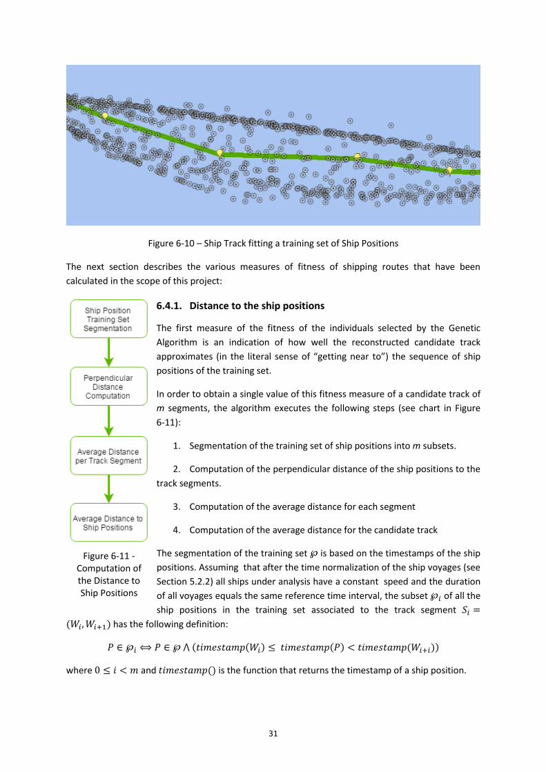
31
Figure 6-10 – Ship Track fitting a training set of Ship Positions
The next section describes the various measures of fitness of shipping routes that have been
calculated in the scope of this project:
6.4.1. Distance to the ship positions
The first measure of the fitness of the individuals selected by the Genetic
Algorithm is an indication of how well the reconstructed candidate track
approximates (in the literal sense of “getting near to”) the sequence of ship
positions of the training set.
In order to obtain a single value of this fitness measure of a candidate track of
m segments, the algorithm executes the following steps (see chart in Figure
6-11):
1. Segmentation of the training set of ship positions into m subsets.
2. Computation of the perpendicular distance of the ship positions to the
track segments.
3. Computation of the average distance for each segment
4. Computation of the average distance for the candidate track
The segmentation of the training set ℘ is based on the timestamps of the ship
positions. Assuming that after the time normalization of the ship voyages (see
Section 5.2.2) all ships under analysis have a constant speed and the duration
of all voyages equals the same reference time interval, the subset ℘𝑖 of all the
ship positions in the training set associated to the track segment 𝑆𝑖 =
(𝑊𝑖,𝑊𝑖+1) has the following definition:
𝑃 ∈ ℘𝑖 ⟺ 𝑃 ∈ ℘ ⋀ (𝑡𝑖𝑚𝑒𝑠𝑡𝑎𝑚𝑝(𝑊𝑖) ≤ 𝑡𝑖𝑚𝑒𝑠𝑡𝑎𝑚𝑝(𝑃) < 𝑡𝑖𝑚𝑒𝑠𝑡𝑎𝑚𝑝(𝑊𝑖+𝑖))
where 0 ≤ 𝑖 < 𝑚 and 𝑡𝑖𝑚𝑒𝑠𝑡𝑎𝑚𝑝() is the function that returns the timestamp of a ship position.
Figure 6-11 - Computation of the Distance to Ship Positions
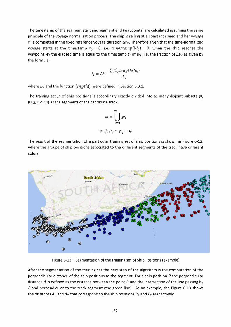
32
The timestamp of the segment start and segment end (waypoints) are calculated assuming the same
principle of the voyage normalization process. The ship is sailing at a constant speed and her voyage
𝑉 is completed in the fixed reference voyage duration ∆𝑡𝑉. Therefore given that the time-normalized
voyage starts at the timestamp 𝑡0 = 0, i.e. 𝑡𝑖𝑚𝑒𝑠𝑡𝑎𝑚𝑝(𝑊0) = 0, when the ship reaches the
waypoint 𝑊𝑖 the elapsed time is equal to the timestamp 𝑡𝑖 of 𝑊𝑖, i.e. the fraction of ∆𝑡𝑉 as given by
the formula:
𝑡𝑖 = ∆𝑡𝑉 ∙∑ 𝑙𝑒𝑛𝑔𝑡ℎ(𝑆𝑘)
𝑖−1𝑘=0
𝐿𝑉
where 𝐿𝑉 and the function 𝑙𝑒𝑛𝑔𝑡ℎ() were defined in Section 6.3.1.
The training set ℘ of ship positions is accordingly exactly divided into as many disjoint subsets ℘𝑖
(0 ≤ 𝑖 < 𝑚) as the segments of the candidate track:
℘ = ⋃ ℘𝑖
𝑚−1
𝑖=0
∀𝑖, 𝑗: ℘𝑖 ∩ ℘𝑗 = ∅
The result of the segmentation of a particular training set of ship positions is shown in Figure 6-12,
where the groups of ship positions associated to the different segments of the track have different
colors.
Figure 6-12 – Segmentation of the training set of Ship Positions (example)
After the segmentation of the training set the next step of the algorithm is the computation of the
perpendicular distance of the ship positions to the segment. For a ship position 𝑃 the perpendicular
distance 𝑑 is defined as the distance between the point 𝑃 and the intersection of the line passing by
𝑃 and perpendicular to the track segment (the green line). As an example, the Figure 6-13 shows
the distances 𝑑1 and 𝑑2 that correspond to the ship positions 𝑃1 and 𝑃2 respectively.
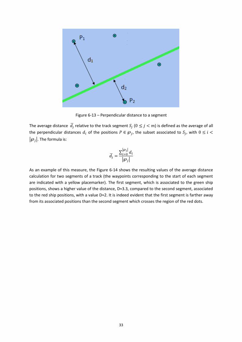
33
Figure 6-13 – Perpendicular distance to a segment
The average distance 𝑑�̅� relative to the track segment 𝑆𝑗 (0 ≤ 𝑗 < 𝑚) is defined as the average of all
the perpendicular distances 𝑑𝑖 of the positions 𝑃 ∈ ℘𝑗, the subset associated to 𝑆𝑗, with 0 ≤ 𝑖 <
|℘𝑗|. The formula is:
𝑑�̅� =∑ 𝑑𝑖
|℘𝑗|
𝑖=0
|℘𝑗|
As an example of this measure, the Figure 6-14 shows the resulting values of the average distance
calculation for two segments of a track (the waypoints corresponding to the start of each segment
are indicated with a yellow placemarker). The first segment, which is associated to the green ship
positions, shows a higher value of the distance, D≈3.3, compared to the second segment, associated
to the red ship positions, with a value D≈2. It is indeed evident that the first segment is farther away
from its associated positions than the second segment which crosses the region of the red dots.
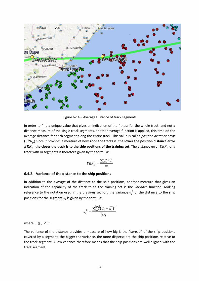
34
Figure 6-14 – Average Distance of track segments
In order to find a unique value that gives an indication of the fitness for the whole track, and not a
distance measure of the single track segments, another average function is applied, this time on the
average distance for each segment along the entire track. This value is called position distance error
(𝐸𝑅𝑅𝑝) since it provides a measure of how good the tracks is: the lower the position distance error
𝑬𝑹𝑹𝒑, the closer the track is to the ship positions of the training set. The distance error 𝐸𝑅𝑅𝑝 of a
track with m segments is therefore given by the formula:
𝐸𝑅𝑅𝑝 =∑ 𝑑�̅�
𝑚−1𝑖=0
𝑚
6.4.2. Variance of the distance to the ship positions
In addition to the average of the distance to the ship positions, another measure that gives an
indication of the capability of the track to fit the training set is the variance function. Making
reference to the notation used in the previous section, the variance 𝜎𝑗2 of the distance to the ship
positions for the segment 𝑆𝑗 is given by the formula:
𝜎𝑗2 =
∑ (𝑑𝑖 − 𝑑�̅�)2|℘𝑗|
𝑖=0
|℘𝑗|
where 0 ≤ 𝑗 < 𝑚.
The variance of the distance provides a measure of how big is the “spread” of the ship positions
covered by a segment: the bigger the variance, the more disperse are the ship positions relative to
the track segment. A low variance therefore means that the ship positions are well aligned with the
track segment.
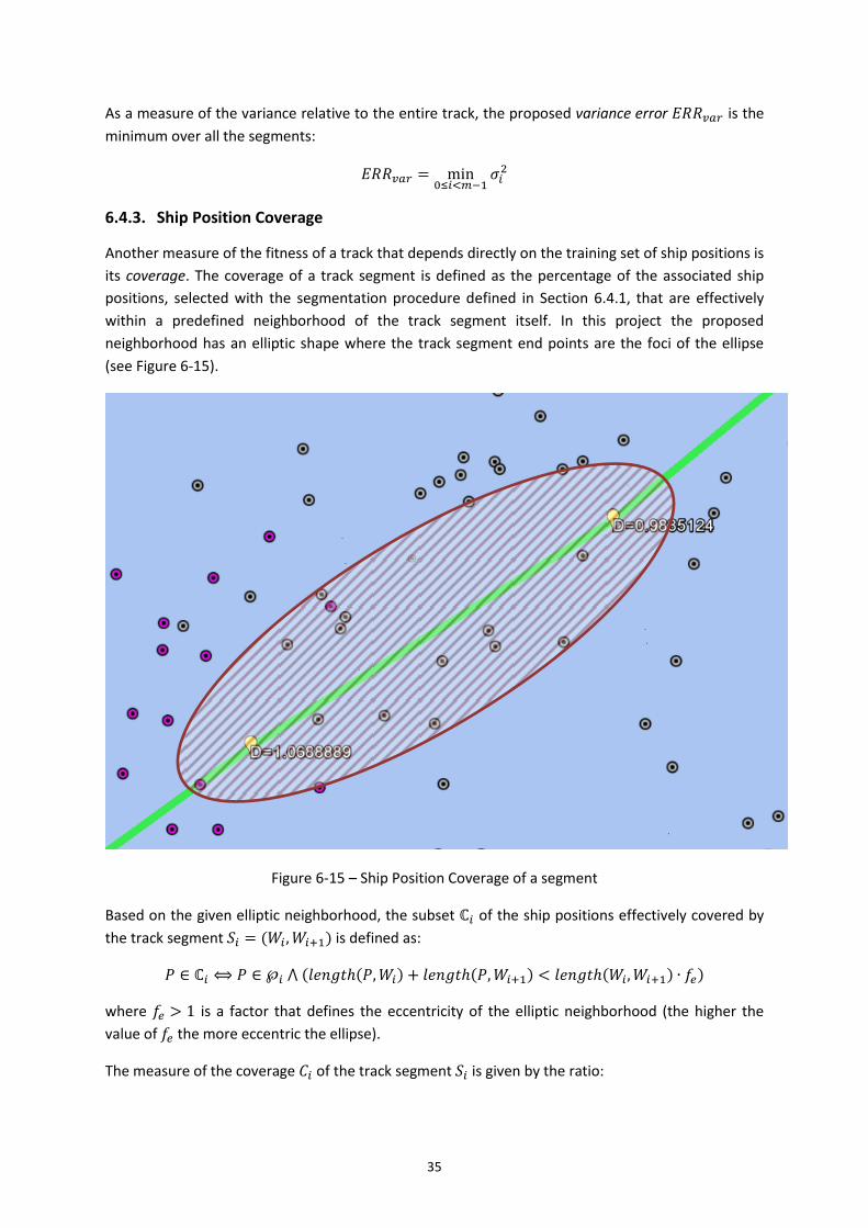
35
As a measure of the variance relative to the entire track, the proposed variance error 𝐸𝑅𝑅𝑣𝑎𝑟 is the
minimum over all the segments:
𝐸𝑅𝑅𝑣𝑎𝑟 = min0≤𝑖<𝑚−1
𝜎𝑖2
6.4.3. Ship Position Coverage
Another measure of the fitness of a track that depends directly on the training set of ship positions is
its coverage. The coverage of a track segment is defined as the percentage of the associated ship
positions, selected with the segmentation procedure defined in Section 6.4.1, that are effectively
within a predefined neighborhood of the track segment itself. In this project the proposed
neighborhood has an elliptic shape where the track segment end points are the foci of the ellipse
(see Figure 6-15).
Figure 6-15 – Ship Position Coverage of a segment
Based on the given elliptic neighborhood, the subset ℂ𝑖 of the ship positions effectively covered by
the track segment 𝑆𝑖 = (𝑊𝑖 ,𝑊𝑖+1) is defined as:
𝑃 ∈ ℂ𝑖 ⟺ 𝑃 ∈ ℘𝑖 ⋀ (𝑙𝑒𝑛𝑔𝑡ℎ(𝑃,𝑊𝑖) + 𝑙𝑒𝑛𝑔𝑡ℎ(𝑃,𝑊𝑖+1) < 𝑙𝑒𝑛𝑔𝑡ℎ(𝑊𝑖,𝑊𝑖+1) ∙ 𝑓𝑒)
where 𝑓𝑒 > 1 is a factor that defines the eccentricity of the elliptic neighborhood (the higher the
value of 𝑓𝑒 the more eccentric the ellipse).
The measure of the coverage 𝐶𝑖 of the track segment 𝑆𝑖 is given by the ratio:
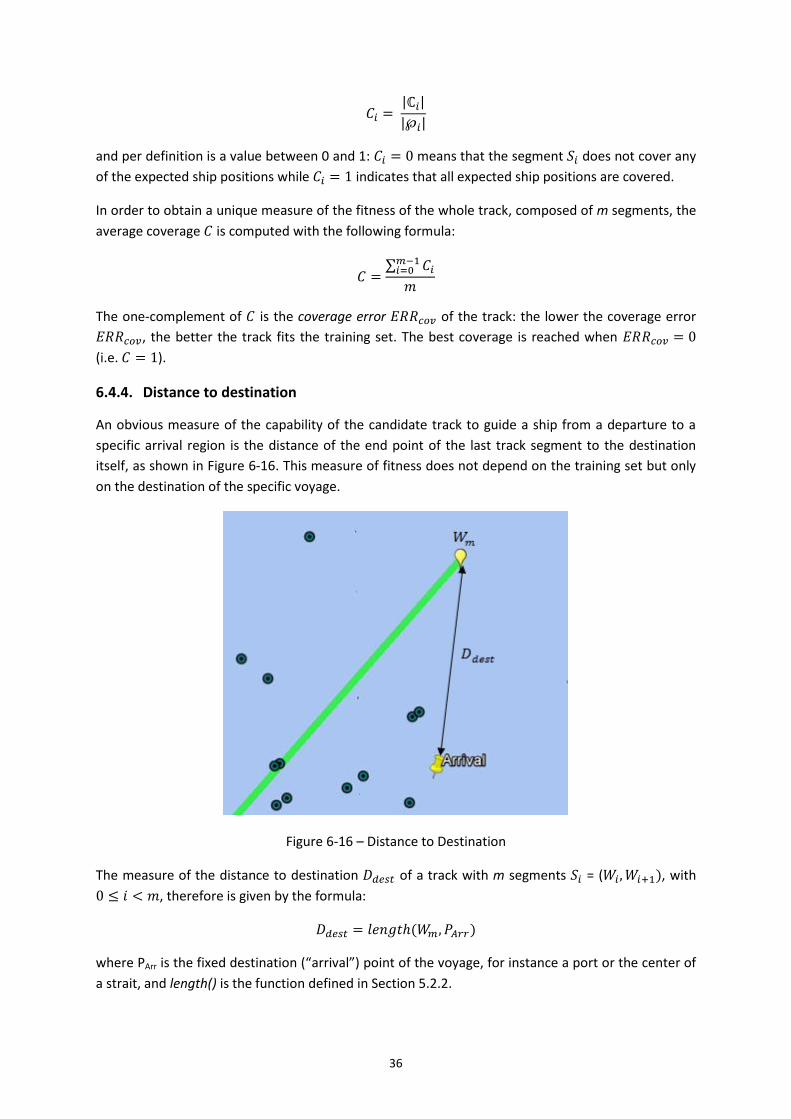
36
𝐶𝑖 = |ℂ𝑖|
|℘𝑖|
and per definition is a value between 0 and 1: 𝐶𝑖 = 0 means that the segment 𝑆𝑖 does not cover any
of the expected ship positions while 𝐶𝑖 = 1 indicates that all expected ship positions are covered.
In order to obtain a unique measure of the fitness of the whole track, composed of m segments, the
average coverage 𝐶 is computed with the following formula:
𝐶 =∑ 𝐶𝑖
𝑚−1𝑖=0
𝑚
The one-complement of 𝐶 is the coverage error 𝐸𝑅𝑅𝑐𝑜𝑣 of the track: the lower the coverage error
𝐸𝑅𝑅𝑐𝑜𝑣, the better the track fits the training set. The best coverage is reached when 𝐸𝑅𝑅𝑐𝑜𝑣 = 0
(i.e. 𝐶 = 1).
6.4.4. Distance to destination
An obvious measure of the capability of the candidate track to guide a ship from a departure to a
specific arrival region is the distance of the end point of the last track segment to the destination
itself, as shown in Figure 6-16. This measure of fitness does not depend on the training set but only
on the destination of the specific voyage.
Figure 6-16 – Distance to Destination
The measure of the distance to destination 𝐷𝑑𝑒𝑠𝑡 of a track with m segments 𝑆𝑖 = (𝑊𝑖,𝑊𝑖+1), with
0 ≤ 𝑖 < 𝑚, therefore is given by the formula:
𝐷𝑑𝑒𝑠𝑡 = 𝑙𝑒𝑛𝑔𝑡ℎ(𝑊𝑚, 𝑃𝐴𝑟𝑟)
where PArr is the fixed destination (“arrival”) point of the voyage, for instance a port or the center of
a strait, and length() is the function defined in Section 5.2.2.
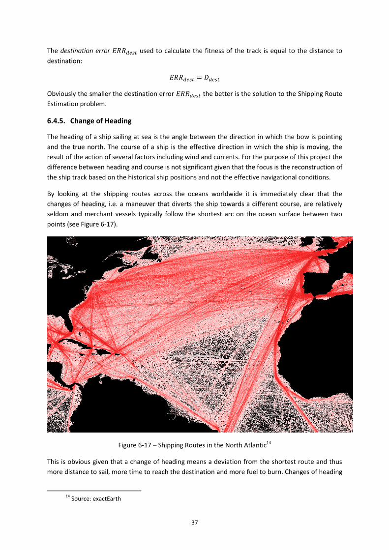
37
The destination error 𝐸𝑅𝑅𝑑𝑒𝑠𝑡 used to calculate the fitness of the track is equal to the distance to
destination:
𝐸𝑅𝑅𝑑𝑒𝑠𝑡 = 𝐷𝑑𝑒𝑠𝑡
Obviously the smaller the destination error 𝐸𝑅𝑅𝑑𝑒𝑠𝑡 the better is the solution to the Shipping Route
Estimation problem.
6.4.5. Change of Heading
The heading of a ship sailing at sea is the angle between the direction in which the bow is pointing
and the true north. The course of a ship is the effective direction in which the ship is moving, the
result of the action of several factors including wind and currents. For the purpose of this project the
difference between heading and course is not significant given that the focus is the reconstruction of
the ship track based on the historical ship positions and not the effective navigational conditions.
By looking at the shipping routes across the oceans worldwide it is immediately clear that the
changes of heading, i.e. a maneuver that diverts the ship towards a different course, are relatively
seldom and merchant vessels typically follow the shortest arc on the ocean surface between two
points (see Figure 6-17).
Figure 6-17 – Shipping Routes in the North Atlantic14
This is obvious given that a change of heading means a deviation from the shortest route and thus
more distance to sail, more time to reach the destination and more fuel to burn. Changes of heading
14
Source: exactEarth
38
are caused by geographical obstacles, like the shoreline or islands, or by more dynamic
circumstances like bad weather conditions or strong currents.
As a consequence of these considerations the average change of heading in correspondence of the
waypoints of the resulting candidate track is another parameter that can be used to measure the
fitness of the shipping route.
The change of heading at a waypoint is defined as the angles between the course of the preceding
segment and the course of the following one.
As already discussed in Chapter 6.2, given a track segment 𝑆𝑖 (0 ≤ 𝑖 < 𝑚) it is possible to calculate
the heading 𝐻𝑖 of the ship sailing along the segment.
If we consider the preceding segment 𝑆𝑖−1 interconnected with 𝑆𝑖 by the waypoint 𝑊𝑖, the change of
heading ∆𝐻𝑖 at the waypoint 𝑊𝑖 is the absolute value of the difference between the old and the new
heading as defined by the formula:
∆𝐻𝑖 = |𝐻𝑖 − 𝐻𝑖−1|
where 0 ≤ 𝑖 < 𝑚.
It is to be noted that for the purpose of this work it is not relevant if the course was changed
towards port (left) or starboard (right). Instead the only interesting parameter is the magnitude of
the change, i.e. its absolute value.
Given a track with 𝑚 segments, in order to characterize it with respect to the overall change of
heading the average change of heading ∆𝐻̅̅ ̅̅ at its 𝑚 − 2 waypoints is computed with the formula:
∆𝐻̅̅ ̅̅ =∑ ∆𝐻𝑖
𝑚−1𝑖=1
𝑚 − 2
Note that at the start and end of the track there is per definition no change of course.
The corresponding heading error 𝐸𝑅𝑅𝐻 is defined as:
𝐸𝑅𝑅𝐻 = ∆𝐻̅̅ ̅̅
The heading error is used as an indication of the low or high magnitude of the changes in the ship
route: the lower the heading error value 𝐸𝑅𝑅𝐻, the less zigzagged the ship route.
Depending on the geographical constraints some significant changes of heading may be necessary,
however over a long distance shipping route, which is the subject of this work, the average change
of heading should be small. Similarly to the distance to destination, this measure of fitness does not
depend directly on the training set but only on the “shape” of the track.
6.5. BUILDING UP THE FITNESS
In a Genetic Algorithm the fitness can be defined as the capability of the individual to solve the
problem under analysis. An individual that makes few and little errors is a good candidate to have
the necessary skills and as a consequence the search for fitness can also be seen as finding the
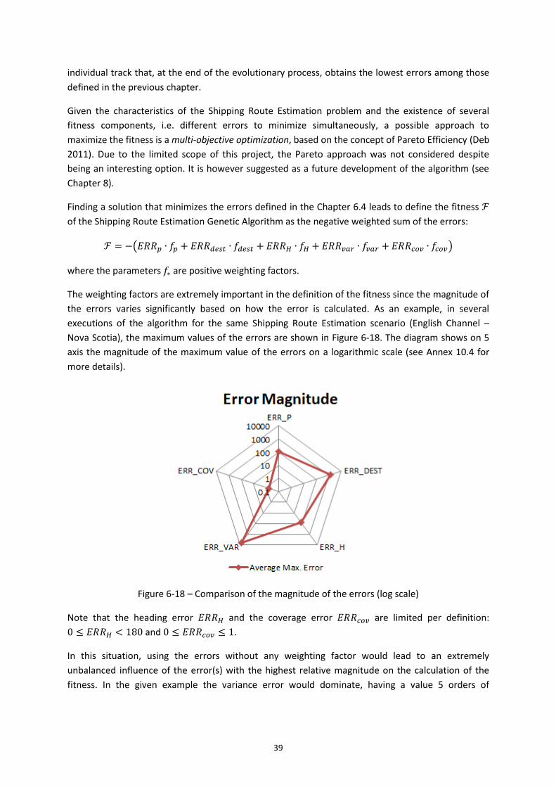
39
individual track that, at the end of the evolutionary process, obtains the lowest errors among those
defined in the previous chapter.
Given the characteristics of the Shipping Route Estimation problem and the existence of several
fitness components, i.e. different errors to minimize simultaneously, a possible approach to
maximize the fitness is a multi-objective optimization, based on the concept of Pareto Efficiency (Deb
2011). Due to the limited scope of this project, the Pareto approach was not considered despite
being an interesting option. It is however suggested as a future development of the algorithm (see
Chapter 8).
Finding a solution that minimizes the errors defined in the Chapter 6.4 leads to define the fitness ℱ
of the Shipping Route Estimation Genetic Algorithm as the negative weighted sum of the errors:
ℱ = −(𝐸𝑅𝑅𝑝 ∙ 𝑓𝑝 + 𝐸𝑅𝑅𝑑𝑒𝑠𝑡 ∙ 𝑓𝑑𝑒𝑠𝑡 + 𝐸𝑅𝑅𝐻 ∙ 𝑓𝐻 + 𝐸𝑅𝑅𝑣𝑎𝑟 ∙ 𝑓𝑣𝑎𝑟 + 𝐸𝑅𝑅𝑐𝑜𝑣 ∙ 𝑓𝑐𝑜𝑣)
where the parameters 𝑓∗ are positive weighting factors.
The weighting factors are extremely important in the definition of the fitness since the magnitude of
the errors varies significantly based on how the error is calculated. As an example, in several
executions of the algorithm for the same Shipping Route Estimation scenario (English Channel –
Nova Scotia), the maximum values of the errors are shown in Figure 6-18. The diagram shows on 5
axis the magnitude of the maximum value of the errors on a logarithmic scale (see Annex 10.4 for
more details).
Figure 6-18 – Comparison of the magnitude of the errors (log scale)
Note that the heading error 𝐸𝑅𝑅𝐻 and the coverage error 𝐸𝑅𝑅𝑐𝑜𝑣 are limited per definition:
0 ≤ 𝐸𝑅𝑅𝐻 < 180 and 0 ≤ 𝐸𝑅𝑅𝑐𝑜𝑣 ≤ 1.
In this situation, using the errors without any weighting factor would lead to an extremely
unbalanced influence of the error(s) with the highest relative magnitude on the calculation of the
fitness. In the given example the variance error would dominate, having a value 5 orders of
40
magnitude higher than the coverage error. Without weights, the other fitness components would be
simply ignored during the fitness evaluation and the selection steps of the evolutionary process.
6.5.1. Setting the Weighting Factors
Since the implemented algorithm is not multi-objective, there is a need to set the values of the
weighting factors in the formula of the fitness ℱ. After many experiments on various shipping route
scenarios (see Chapter 7.2) following a basic trial and error approach, the most adequate weighting
factors were found to be the following:
𝑓𝑝 = 10
𝑓𝑑𝑒𝑠𝑡 = 10−2
𝑓𝐻 = 1
To avoid too many variables in the final assessment of the algorithm, the coverage and variance
errors were calculated but not included in the fitness formula and thus 𝑓𝑣𝑎𝑟 = 𝑓𝑐𝑜𝑣 = 0.
The complete formula to compute the fitness ℱ in the Genetic Algorithm for Shipping Route
Estimation is:
ℱ = −(10 ∙ 𝐸𝑅𝑅𝑝 +𝐸𝑅𝑅𝑑𝑒𝑠𝑡
100+ 𝐸𝑅𝑅𝐻)
The assessment of the results obtained with this formula on the use case scenarios is presented in
Chapter 7.2.
6.6. ECJ: AN EVOLUTIONARY COMPUTATION RESEARCH SYSTEM
The ECJ Java library (Luke, 2000) was chosen in order to implement the Machine Learning system
that provides a solution to the Shipping Route Estimation problem. ECJ is a very comprehensive and
efficient programming framework that allows developing customized Genetic Algorithms. The
methods of existing ECJ Java classes can be overwritten and the execution of the evolution process is
driven by means of a set of configuration parameters. ECJ covers a great number of Genetic
Algorithms and Genetic Programming techniques. It also provides “handlers” that give the
programmer the possibility to monitor and control the performance of the software.
ECJ supports several types of representations for individuals and evolution strategies that can be
used to tackle in a very quick way many types of problems.
6.6.1. Genetic Algorithm Configuration Parameters
The ECJ library requires a specific configuration file that sets all the necessary parameters of the
Genetic Algorithm. All the relevant parameters in the ECJ library configuration file are described in
this section.
The majority of the configuration parameters are fixed and common for all shipping route scenarios.
The first is the number of individuals in the population of the Genetic Algorithm which equals 1000.
This population size provides a sufficient amount of initial variability with acceptable results. The
likelihood of crossover is 0.5 (50%) and the mutation probability equals 0.2 (20%). Both values were
found with a trial and error approach by running the algorithm with several combinations of
41
high/low crossover and mutation probability and by checking the outcome in different scenarios.
The selection method before crossover is the “Tournament” with groups of 10 individuals. This
configuration provides good solutions in an acceptable amount of computation time.
In addition to the fixed configuration parameters mentioned previously, some parameters have to
be fine-tuned according to the specific shipping route scenario to be analyzed. The first is the
number of generations bred before the termination of the evolution process. A typical value is 100
but this can be higher if the route has one or more changes of heading which require more
“evolution time” to reach an acceptable solution. Other two parameters that are related to the
number of turns in the route are the minimum and maximum size of the genome. The genome size
corresponds to the number of track segments, i.e. displacements, and it is evident that the more
course changes, the more segments are needed to find a good solution. The final parameter to be
adjusted is the maximum absolute value of the gene, which is expressed in degrees in latitude or
longitude. The default value of 10 degrees may need to be reduced if the length of the shipping
route is relatively small (see scenario in Section 7.2.3).
The complete configuration file used during the project is available in Annex 10.3.

42
7. RESULTS
7.1. SHIPPING ROUTE ESTIMATION IN PRACTICE
The Machine Learning system developed in this project was applied to several scenarios, indicated
by the expert user consulted during the requirement analysis phase. The main objective is to assess
the viability of such an approach to solve the Shipping Route Estimation problem and identify the
areas which require further research and experimenting.
It is interesting to see how the Genetic Algorithm effectively “learns” during its execution on a real
training dataset. As an example, the following snapshots (see Figure 7-1 to Figure 7-5) show the
scenario “Channel – Nova Scotia”. This is one of the most operated routes in the North Atlantic and
the vessel tracking systems provide a good amount of ship positions to be used as a training set.
Snapshots of the best individual of the population taken from generation 0 to 80 show how the
algorithm is gradually capable of selecting a candidate track, indicated by the green segments, that
becomes more and more “fit” for the purpose of solving the specific problem. After the last
generation a track is found that connects the two Ocean regions by imitating what many ships have
actually done in the past.
Figure 7-1 – Track Evolution, Generation 0
The best individual of the first generation is almost a random track with no resemblance whatsoever to a shipping route.
Figure 7-2 – Track Evolution, Generation 10
The 10th generation shows an initial attempt to go in the westward direction. On waypoint 4 however there is a huge change of heading (almost 180 degrees) and the ship sails on an opposite course.
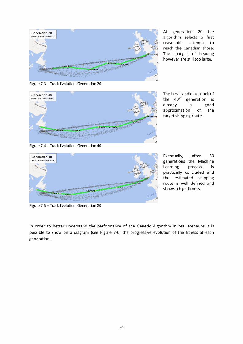
43
Figure 7-3 – Track Evolution, Generation 20
At generation 20 the algorithm selects a first reasonable attempt to reach the Canadian shore. The changes of heading however are still too large.
Figure 7-4 – Track Evolution, Generation 40
The best candidate track of the 40th generation is already a good approximation of the target shipping route.
Figure 7-5 – Track Evolution, Generation 80
Eventually, after 80 generations the Machine Learning process is practically concluded and the estimated shipping route is well defined and shows a high fitness.
In order to better understand the performance of the Genetic Algorithm in real scenarios it is
possible to show on a diagram (see Figure 7-6) the progressive evolution of the fitness at each
generation.

44
Figure 7-6 – Fitness chart (sample)
The diagram depicts on the y-axis the fitness value of the best individual of each of the first 50
generations during the execution of the Machine Learning process for the same Shipping Route
Estimation scenario (Channel – Nova Scotia). After a steep increase and a punctual reduction around
generation 5, the subsequent trend is a steady growth of the fitness value towards an individual
which optimally matches the quality criteria.
7.1.1. Performance
The data ETL process has taken up most of the resources of this project in terms of preparation time
and computation power. The conversion of the AIS raw data needs a series of automatic scripts
running for several hours (days in some cases) and the large amount of ship tracking data requires a
considerable storage and pre-processing effort (approximately one day per scenario). However the
preparation of the data and the loading procedure of the relevant ship positions into the data mart
are to be done only once. In an operational system, this task would be planned in advance and
executed a few times per years.
On the other side one of the main characteristics of the Shipping Route Estimation prototype system
developed in this project is the possibility to find a candidate track in a relatively short amount of
time which in all scenarios was below 10 minutes on a standard laptop.
7.2. USE CASE SCENARIOS
This chapter shows the output of the Shipping Route Estimation prototype system applied to some
representative use case scenarios.
7.2.1. Lanzarote-Natal Route
The Lanzarote-Natal shipping route analyzed in the project is a major passage of the Atlantic Ocean
that connects Europe to South America. The typical route is 2,500 nautical miles long (4,700 km) and
requires very limited changes of course. There are neither major geographic obstacles nor hazardous
weather conditions throughout the year.
-600-500-400-300-200-100
0
G_0
G_4
G_8
G_1
2
G_1
6
G_2
0
G_2
4
G_2
8
G_3
2
G_3
6
G_4
0
G_4
4
G_4
8
Fitn
ess
Generation
Fitness Evolution
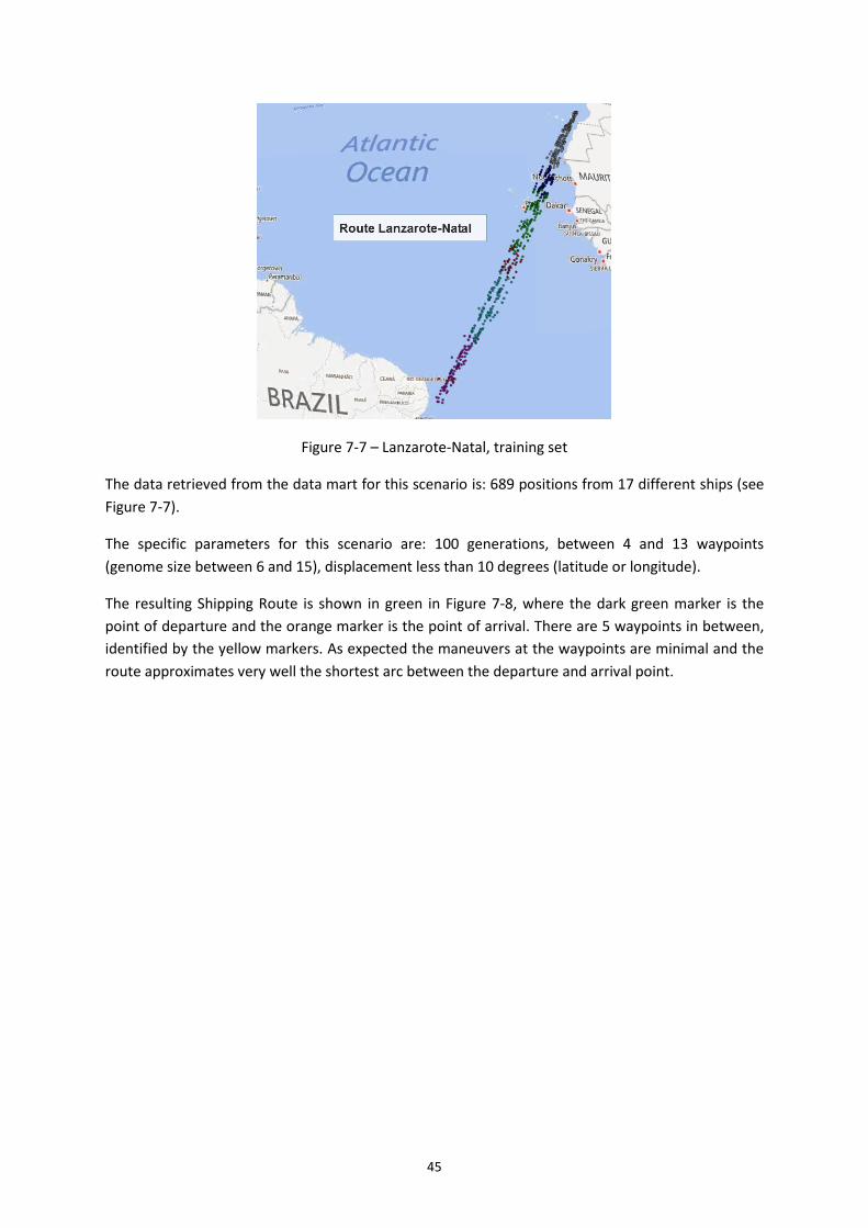
45
Figure 7-7 – Lanzarote-Natal, training set
The data retrieved from the data mart for this scenario is: 689 positions from 17 different ships (see
Figure 7-7).
The specific parameters for this scenario are: 100 generations, between 4 and 13 waypoints
(genome size between 6 and 15), displacement less than 10 degrees (latitude or longitude).
The resulting Shipping Route is shown in green in Figure 7-8, where the dark green marker is the
point of departure and the orange marker is the point of arrival. There are 5 waypoints in between,
identified by the yellow markers. As expected the maneuvers at the waypoints are minimal and the
route approximates very well the shortest arc between the departure and arrival point.
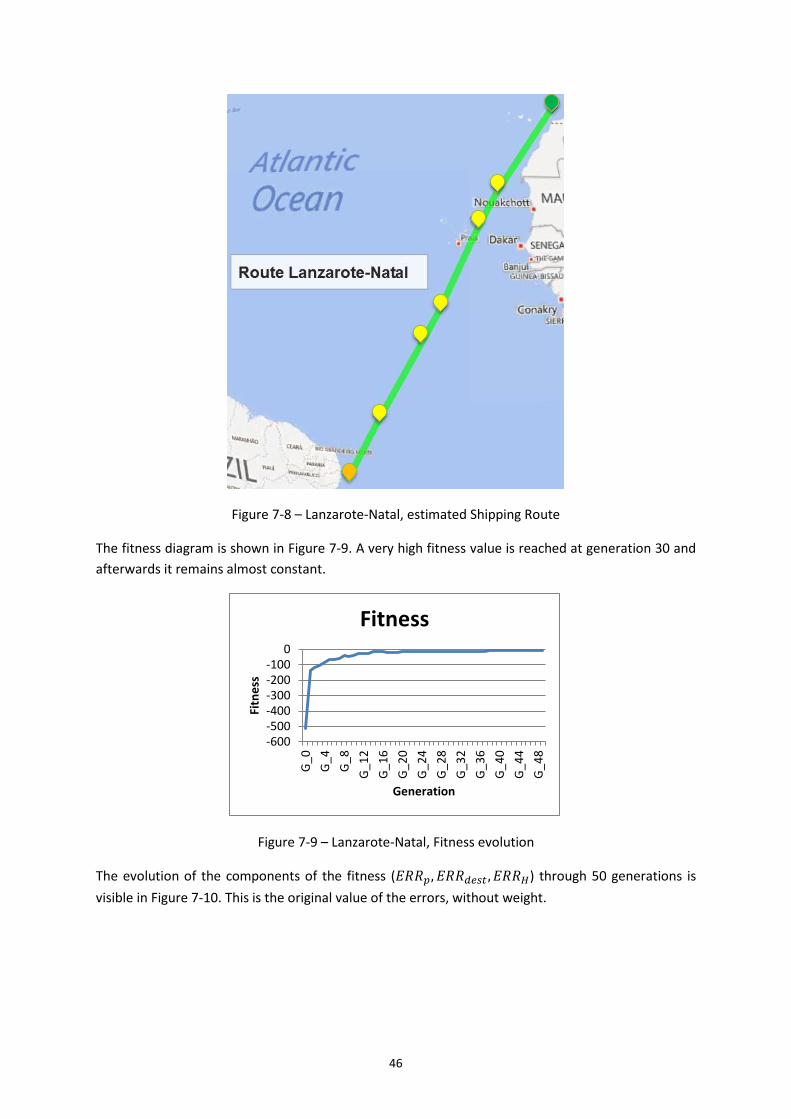
46
Figure 7-8 – Lanzarote-Natal, estimated Shipping Route
The fitness diagram is shown in Figure 7-9. A very high fitness value is reached at generation 30 and
afterwards it remains almost constant.
Figure 7-9 – Lanzarote-Natal, Fitness evolution
The evolution of the components of the fitness (𝐸𝑅𝑅𝑝, 𝐸𝑅𝑅𝑑𝑒𝑠𝑡 , 𝐸𝑅𝑅𝐻) through 50 generations is
visible in Figure 7-10. This is the original value of the errors, without weight.
-600-500-400-300-200-100
0
G_0
G_4
G_8
G_1
2
G_1
6
G_2
0
G_2
4
G_2
8
G_3
2
G_3
6
G_4
0
G_4
4
G_4
8
Fitn
ess
Generation
Fitness

47
Figure 7-10 – Lanzarote-Natal, Fitness Components
Figure 7-11 shows instead the weighted values between generation 20 and generation 50. In this
diagram it can be seen that the 3 fitness components have comparable values and there is a
common overall steady decrease.
Figure 7-11 – Lanzarote-Natal, Fitness Components (weighted values)
Remarks
In the scenario of a ship crossing the Atlantic towards South-America, the Genetic Algorithm
estimates the most operated route with a good outcome. The three error components are
minimized as expected in a relatively small number of generations and the resulting route fits well
the underlying training set. The number of waypoints could be further reduced, during a post-
processing phase, by eliminating maneuvers with a very small change of heading and in open sea
that can be considered unnecessary.
0
100
200
300
400
500
600
G_0
G_3
G_6
G_9
G_1
2
G_1
5
G_1
8
G_2
1
G_2
4
G_2
7
G_3
0
G_3
3
G_3
6
G_3
9
G_4
2
G_4
5
G_4
8
Erro
r V
alu
es
Generation
Fitness Components
ERR_P
ERR_DEST
ERR_H
0
1
2
3
4
5
6
7
8
G_2
0
G_2
2
G_2
4
G_2
6
G_2
8
G_3
0
G_3
2
G_3
4
G_3
6
G_3
8
G_4
0
G_4
2
G_4
4
G_4
6
G_4
8
Erro
r V
alu
e (
we
igh
ted
)
Generation
Fitness Components
W_ERR_P
W_ERR_DEST
W_ERR_H
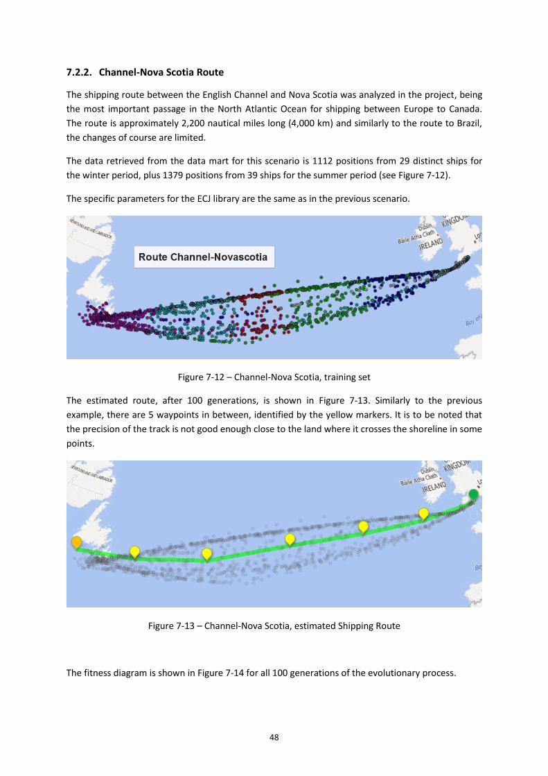
48
7.2.2. Channel-Nova Scotia Route
The shipping route between the English Channel and Nova Scotia was analyzed in the project, being
the most important passage in the North Atlantic Ocean for shipping between Europe to Canada.
The route is approximately 2,200 nautical miles long (4,000 km) and similarly to the route to Brazil,
the changes of course are limited.
The data retrieved from the data mart for this scenario is 1112 positions from 29 distinct ships for
the winter period, plus 1379 positions from 39 ships for the summer period (see Figure 7-12).
The specific parameters for the ECJ library are the same as in the previous scenario.
Figure 7-12 – Channel-Nova Scotia, training set
The estimated route, after 100 generations, is shown in Figure 7-13. Similarly to the previous
example, there are 5 waypoints in between, identified by the yellow markers. It is to be noted that
the precision of the track is not good enough close to the land where it crosses the shoreline in some
points.
Figure 7-13 – Channel-Nova Scotia, estimated Shipping Route
The fitness diagram is shown in Figure 7-14 for all 100 generations of the evolutionary process.
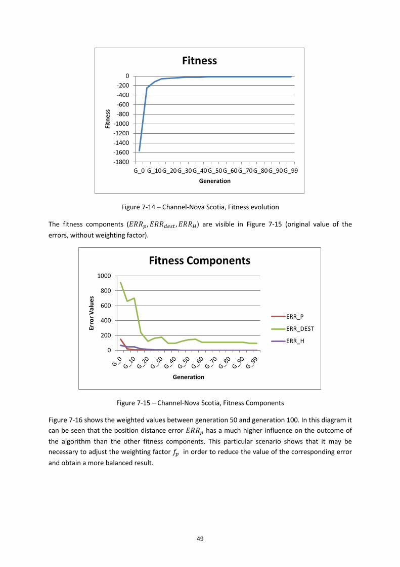
49
Figure 7-14 – Channel-Nova Scotia, Fitness evolution
The fitness components (𝐸𝑅𝑅𝑝, 𝐸𝑅𝑅𝑑𝑒𝑠𝑡 , 𝐸𝑅𝑅𝐻) are visible in Figure 7-15 (original value of the
errors, without weighting factor).
Figure 7-15 – Channel-Nova Scotia, Fitness Components
Figure 7-16 shows the weighted values between generation 50 and generation 100. In this diagram it
can be seen that the position distance error 𝐸𝑅𝑅𝑝 has a much higher influence on the outcome of
the algorithm than the other fitness components. This particular scenario shows that it may be
necessary to adjust the weighting factor 𝑓𝑝 in order to reduce the value of the corresponding error
and obtain a more balanced result.
-1800
-1600
-1400
-1200
-1000
-800
-600
-400
-200
0
G_0 G_10 G_20 G_30 G_40 G_50 G_60 G_70 G_80 G_90 G_99
Fitn
ess
Generation
Fitness
0
200
400
600
800
1000
Erro
r V
alu
es
Generation
Fitness Components
ERR_P
ERR_DEST
ERR_H
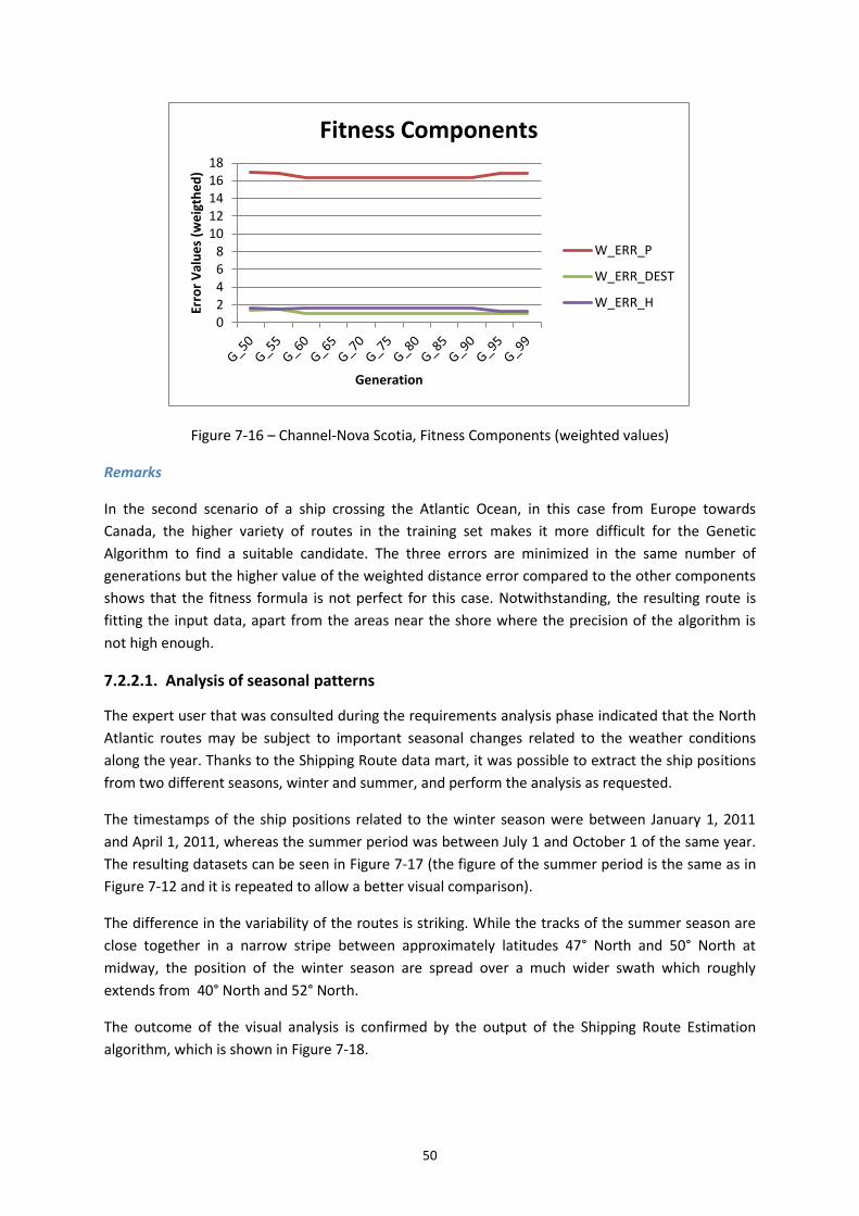
50
Figure 7-16 – Channel-Nova Scotia, Fitness Components (weighted values)
Remarks
In the second scenario of a ship crossing the Atlantic Ocean, in this case from Europe towards
Canada, the higher variety of routes in the training set makes it more difficult for the Genetic
Algorithm to find a suitable candidate. The three errors are minimized in the same number of
generations but the higher value of the weighted distance error compared to the other components
shows that the fitness formula is not perfect for this case. Notwithstanding, the resulting route is
fitting the input data, apart from the areas near the shore where the precision of the algorithm is
not high enough.
7.2.2.1. Analysis of seasonal patterns
The expert user that was consulted during the requirements analysis phase indicated that the North
Atlantic routes may be subject to important seasonal changes related to the weather conditions
along the year. Thanks to the Shipping Route data mart, it was possible to extract the ship positions
from two different seasons, winter and summer, and perform the analysis as requested.
The timestamps of the ship positions related to the winter season were between January 1, 2011
and April 1, 2011, whereas the summer period was between July 1 and October 1 of the same year.
The resulting datasets can be seen in Figure 7-17 (the figure of the summer period is the same as in
Figure 7-12 and it is repeated to allow a better visual comparison).
The difference in the variability of the routes is striking. While the tracks of the summer season are
close together in a narrow stripe between approximately latitudes 47° North and 50° North at
midway, the position of the winter season are spread over a much wider swath which roughly
extends from 40° North and 52° North.
The outcome of the visual analysis is confirmed by the output of the Shipping Route Estimation
algorithm, which is shown in Figure 7-18.
02468
1012141618
Erro
r V
alu
es
(we
igth
ed
)
Generation
Fitness Components
W_ERR_P
W_ERR_DEST
W_ERR_H

51
Figure 7-17 – Winter-summer comparison of the Channel-Nova Scotia training sets
Figure 7-18 – Estimated summer and winter routes
The estimated route for the winter season reaches more southern latitudes, indicating that the
majority of the ships in this period of the year avoid the more dangerous subpolar regions.
summer route
winter route
winter
summer
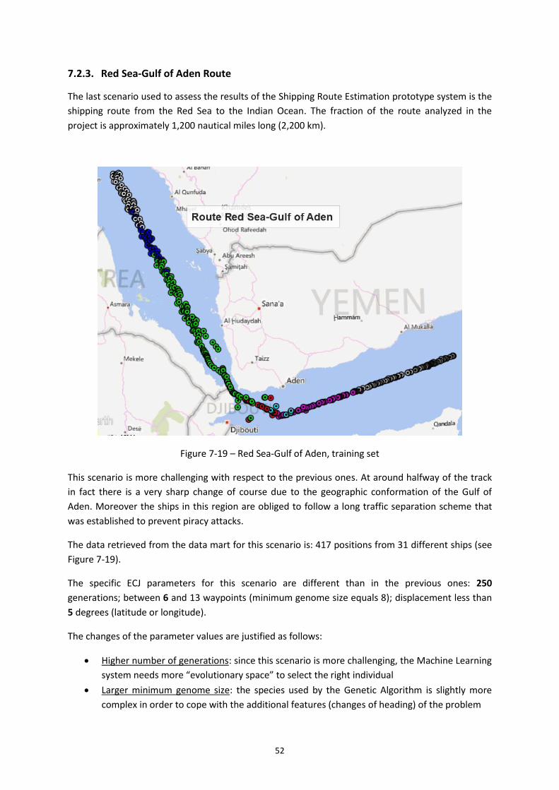
52
7.2.3. Red Sea-Gulf of Aden Route
The last scenario used to assess the results of the Shipping Route Estimation prototype system is the
shipping route from the Red Sea to the Indian Ocean. The fraction of the route analyzed in the
project is approximately 1,200 nautical miles long (2,200 km).
Figure 7-19 – Red Sea-Gulf of Aden, training set
This scenario is more challenging with respect to the previous ones. At around halfway of the track
in fact there is a very sharp change of course due to the geographic conformation of the Gulf of
Aden. Moreover the ships in this region are obliged to follow a long traffic separation scheme that
was established to prevent piracy attacks.
The data retrieved from the data mart for this scenario is: 417 positions from 31 different ships (see
Figure 7-19).
The specific ECJ parameters for this scenario are different than in the previous ones: 250
generations; between 6 and 13 waypoints (minimum genome size equals 8); displacement less than
5 degrees (latitude or longitude).
The changes of the parameter values are justified as follows:
Higher number of generations: since this scenario is more challenging, the Machine Learning
system needs more “evolutionary space” to select the right individual
Larger minimum genome size: the species used by the Genetic Algorithm is slightly more
complex in order to cope with the additional features (changes of heading) of the problem
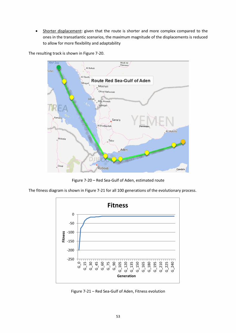
53
Shorter displacement: given that the route is shorter and more complex compared to the
ones in the transatlantic scenarios, the maximum magnitude of the displacements is reduced
to allow for more flexibility and adaptability
The resulting track is shown in Figure 7-20.
Figure 7-20 – Red Sea-Gulf of Aden, estimated route
The fitness diagram is shown in Figure 7-21 for all 100 generations of the evolutionary process.
Figure 7-21 – Red Sea-Gulf of Aden, Fitness evolution
-250
-200
-150
-100
-50
0
G_0
G_1
5
G_3
0
G_4
5
G_6
0
G_7
5
G_9
0
G_1
05
G_1
20
G_1
35
G_1
50
G_1
65
G_1
80
G_1
95
G_2
10
G_2
25
G_2
40
Fitn
ess
Generation
Fitness
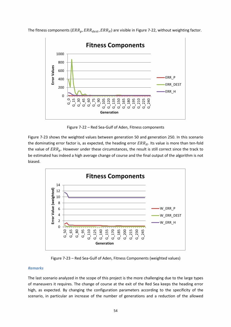
54
The fitness components (𝐸𝑅𝑅𝑝, 𝐸𝑅𝑅𝑑𝑒𝑠𝑡 , 𝐸𝑅𝑅𝐻) are visible in Figure 7-22, without weighting factor.
Figure 7-22 – Red Sea-Gulf of Aden, Fitness components
Figure 7-23 shows the weighted values between generation 50 and generation 250. In this scenario
the dominating error factor is, as expected, the heading error 𝐸𝑅𝑅𝐻. Its value is more than ten-fold
the value of 𝐸𝑅𝑅𝑝. However under these circumstances, the result is still correct since the track to
be estimated has indeed a high average change of course and the final output of the algorithm is not
biased.
Figure 7-23 – Red Sea-Gulf of Aden, Fitness Components (weighted values)
Remarks
The last scenario analyzed in the scope of this project is the more challenging due to the large types
of maneuvers it requires. The change of course at the exit of the Red Sea keeps the heading error
high, as expected. By changing the configuration parameters according to the specificity of the
scenario, in particular an increase of the number of generations and a reduction of the allowed
0
200
400
600
800
1000
G_0
G_1
5
G_3
0
G_4
5
G_6
0
G_7
5
G_9
0
G_1
05
G_1
20
G_1
35
G_1
50
G_1
65
G_1
80
G_1
95
G_2
10
G_2
25
G_2
40
Erro
r V
alu
es
Generation
Fitness Components
ERR_P
ERR_DEST
ERR_H
0
2
4
6
8
10
12
14
G_5
0
G_6
5
G_8
0
G_9
5
G_1
10
G_1
25
G_1
40
G_1
55
G_1
70
G_1
85
G_2
00
G_2
15
G_2
30
G_2
45
Erro
r V
alu
e (
we
igh
ted
)
Generation
Fitness Components
W_ERR_P
W_ERR_DEST
W_ERR_H

55
maximum displacement, the resulting route fits well the training set, especially in correspondence of
the turn and the traffic separation scheme.
7.3. EXPERT ASSESSMENT
The results of the project and the calculated shipping routes have been shown to an expert in the
Maritime domain. The expert worked many years as a captain of a tanker ship and he was requested
to assess the validity of such a shipping route estimator for real world applications like route
planning and anomaly detection.
The main remarks of the expert are summarized as follows:
The Shipping Route Estimation system is a practical tool to provide an indicative route
between two ocean regions based on historical information; for straightforward scenarios
the outcome of the algorithm can be used to compare the voyage passage plan with the
recommended route and thereafter to monitor the performance of the ship against the
reference track between waypoints.
The seasonal pattern analysis confirms the implicit knowledge of the shipmaster about the
differences in the routes between summer and winter caused by variable weather
conditions; the estimated seasonal route can be used as a guideline of the recommended
track; adding the “Ship Type” criteria will further improve the usability of the tool as there is
a direct relationship between ship type and capability to face adverse weather conditions.
The tool should take as an input the geographic obstacles and other fixed constraints, such
as restricted areas and traffic separation schemes, to be used as an a priori knowledge to
support and correct, if necessary, the learning process of the machine; this is essential for an
effective operational application, since mariners take into great consideration all these
factors and including them would increase the confidence in this technology.
As a future work, it would be interesting to see if the outcome improves with more
computation power, over a longer period of time and on a larger database.
7.4. MARITIME SAFETY APPLICATIONS
With regard to the possibility to use the Shipping Route Estimation service for Maritime Safety
purposes, the following main applications were identified:
Ship monitoring based on the estimated Shipping Route
Support to Shipping Route planning
Historical analysis of Shipping Routes patterns
It is to be noted that the precision and reliability of the algorithm developed during the project are
not sufficient to ensure the required quality for real navigation purposes. The Shipping Route
Estimation prototype is not an autopilot that can steer a ship from a port to another. The output of
the Genetic Algorithm however can be one of the sources of information for a Decision Support
System to alert or guide a shipmaster, a VTS operator, a shipping company or any other stakeholder
in the Maritime Safety domain.

56
7.4.1. Ship Monitoring and Alerting
A Ship Monitoring system aims at tracking ships in real-time and providing information on their
current positions, their navigational status, the type of cargo, etc. The tracking of ships may be
worldwide or limited to a specific ocean region. Most recent Ship Monitoring systems combine ship
tracking with an automatic monitoring of the ship behavior and alerting in case of anomalies.
A ship monitoring system is, in some cases, aware of the destination of a ship, for instance based on
AIS message type 5 or other sources of information (mandatory reporting systems, a dispatch from
the shipping company, etc.).
The knowledge of the destination of a ship and the nominal shipping route between the ocean
regions of departure and arrival allow the setting an automatic alerting tool that checks if there is
any significant deviation of the ship from the expected course.
Figure 7-24 – Alert triggered by an anomalous deviation from the expected course
In the example shown in Figure 7-24 a ship is sailing westward from Europe to Canada on the
expected route estimated for the scenario Channel – Nova Scotia. The expected route is the light
green line and the ship track is in white. In order to cater for the route variation mentioned in
Section 7.2.2.1 a corridor is defined along the expected route (dark green). The width of the corridor
is to be defined according to the seasonal patterns: the more variability in the routes, the wider the
corridor. The tool would raise an alert of type “Route Deviation Anomaly” as soon as one position is
received outside of the corridor. In such a case an operator may be instructed to perform further
checks and verify the situation with the shipmaster or the shipping company.
7.4.2. Route Planning
Route planning is the activity performed by a shipmaster before starting any new voyage in order to
calculate the best route towards a specific destination port or to a particular ocean region. The
traditional methods to plan a sea route are based mainly on distance calculation. The relevant
geographic features, as the shoreline, are considered as well as the weather conditions.

57
The Shipping Route Estimation algorithm could be used as a complementary tool to support this
planning task, with the advantage that it takes into account the real voyages, successfully completed
by many ships in the previous years and during the same period of time. The output of the Genetic
Algorithm could be used to validate the route calculated with the standard method as well as
proposing alternative, possibly safer, routes that were already operated in the past.
7.4.3. Route Pattern Analysis
The analysis of the changes in the most operated shipping routes of merchant vessels in a specific
region over a longer period of time has been performed in several projects. One of the most recent
regards the situation in the Indian Ocean, particularly off the coast of Somalia, where piracy was a
major security concern in the past years. The identification of new shipping route patterns may be
interesting for the authorities and the shipping companies. This is the case when, for instance, the
new routes affect environmental sensitive areas.
The Shipping Route Estimation algorithm can be used for the purpose of pattern analysis as it was
shown in Section 7.2.2.1. Estimating a route over several consecutive period of time may show
trends that indicate a different behavior of the merchant fleet and help preventing long-term side
effects on the environment and on other human activities in the area, e.g. fishing.
58
8. CONCLUSIONS AND FUTURE WORK
A new Genetic Algorithm for the estimation of Shipping Routes has been developed in the scope of
this project. The work mainly focused on major routes between two ocean regions, over 1000
nautical miles long and located in open sea. The objective was to assess if the analysis of the
archived positions of ships can provide a practical estimation of the most operated route connecting
two ocean regions.
The input data was collected from two long-range ship tracking systems, with worldwide coverage:
LRIT and Sat-AIS. The data was kindly provided by the European Maritime Safety Agency (EMSA), the
Norwegian Maritime Administration, the Maltese Maritime Administration, the Italian Coast Guard,
and by the private company exactEarth, a leading provider of ship tracking services.
The most time consuming phases of the project were the design and development of the process of
extracting, transforming and loading (ETL) the input data into the Shipping Route Estimation
database. The large amount of ship position records and the need to quickly access and load the
data during the subsequent analysis phase required the implementation of an intermediate Staging
Area used for data cleansing and filtering. A Data Mart was designed and deployed to store the Ship
Track information in the spatial and temporal dimensions for efficient data retrieval.
The problem of estimating the Shipping Route was modelled as the search for a ship track with fixed
point of departure and a variable number of waypoints, represented as a sequence of displacement
in the latitude/longitude two-dimensional plane. The criteria selected to assess the quality (fitness)
of a solution were the following: the distance of the track from the ship positions of the training set,
the estimated changes of heading and the distance of the last point of the track from the final
destination of the shipping route. A multi-objective optimization approach, based on the Pareto
efficiency, was not followed in favor of a more simple fitness formula with weighting factors.
The corresponding Genetic Algorithm for the optimization of the fitness was implemented with the
open-source ECJ library. The quality of the results was heavily dependent on the weighting factors
used to compute the fitness of a solution and other configuration parameters as the total number of
generations and the maximum displacement allowed between the track waypoints. The fine-tuning
of the algorithm with a manual trial and error approach required a lot of effort. This task could be
improved by executing the algorithm with different configurations in an automatic way, for instance
with a script running overnight, and reviewing all the results at once.
The estimated shipping routes for three scenarios (North and Equatorial Atlantic crossing and Red
Sea/Gulf of Aden) have been evaluated by an expert. The outcome is considered a satisfactory
indicative route between the two ocean regions under analysis. Although the service provided by
the system developed in this project is not enough precise for practical navigational purposes
onboard a ship, it can be used as a reference for detection of anomalous deviations of a vessel from
the expected course or as an additional source of information for route planning. An additional
application is the pattern analysis over several years to identify trends or seasonal changes in the
main shipping routes.
The effort required to complete the data pre-processing task, including the data cleansing, was
underestimated and it took more time than expected. Despite the difficulties, the result was
59
satisfactory and the performance of the Data Mart allowed completing the extraction of the training
set and the analysis of a particular shipping route scenario in less than 1 hour. The following
improvements of the pre-processing phase were not implemented due to time constraints: the
inclusion of the Ship Type in the selection of the ship tracks and the automatic removal of outliers
which was done manually. In particular the use of the dimension “Ship Type” could improve the
quality of the results since different classes of ships have a different behavior on some routes.
8.1. FUTURE DEVELOPMENT
The use of Genetic Algorithms for the problem of estimating shipping routes is not an operational
technology yet. Future work on this field could be the engineering of the concepts and the prototype
developed in this project and the further validation of the proposed fitness formula on many more
different scenarios and training sets.
The inclusion of the Ship Type as an additional dimension of the data analysis is considered by the
expert as an important enhancement, to be assessed in a future development of the algorithm
particularly with regard to the detection of seasonal behavior patterns.
The validation approach of the project should be improved with other quantitative measures of the
quality of the estimated routes and the comparison with of other Shipping Route Estimation
techniques. A post-processing module could also identify unnecessary maneuvers which change the
course of the ship by a negligible amount and thus are redundant.
The approach of building up a fitness which is a sum of several components (error minimization)
could be improved by using the concept of Pareto efficiency. A Genetic Algorithm for the multi-
objective optimization based on two or more criteria could be implemented with the same ECJ
framework and the results compared on the scenarios analyzed in this project.
Finally the Shipping Route Estimation algorithm could be significantly enhanced with the inclusion of
additional criteria that would guide the evolutionary process. The algorithm should also consider the
local geographic and maritime feature of the routes: the passage of straits, the minimum distance to
the shore, the mandatory use of traffic separation schemes, the avoidance of environmental or
security sensitive areas. The individual tracks that do not match these more stringent navigation
constraints would be eliminated from the population and a better and more practical result would
be achieved.
60
9. BIBLIOGRAPHY
Fernandez Arguedas, V., Pallotta, G., & Vespe, M. (2014, July). Automatic generation of geographical networks for maritime traffic surveillance. In Information Fusion (FUSION), 2014 17th International Conference on (pp. 1-8). IEEE.
Chen, C. H., Khoo, L. P., Chong, Y. T., & Yin, X. F. (2014). Knowledge discovery using genetic algorithm for maritime situational awareness. Expert Systems with Applications, 41(6), 2742-2753.
Deb, K. (2011). Multi-objective optimisation using evolutionary algorithms: an introduction. In Multi-objective evolutionary optimisation for product design and manufacturing (pp. 3-34). Springer London.
Goldberg, D. E., & Holland, J. H. (1988). Genetic algorithms and machine learning. Machine learning, 3(2), 95-99.
International Maritime Organization - IMO (2012). International Shipping Facts and Figures – Information Resources on Trade , Safety , Security , Environment.
International Maritime Organization - IMO (2004). Consolidated text of the International Convention of Safety of Life at Sea, 1974, and its Protocol of 1988: articles, annexes and certificates. IMO, London.
Kazemi, S., Abghari, S., Lavesson, N., Johnson, H., & Ryman, P. (2013). Open data for anomaly detection in maritime surveillance. Expert Systems with Applications, 40(14), 5719-5729.
Krata, P., & Szlapczynska, J. (2011). 21. Weather Hazard Avoidance in Modeling Safety of Motor-driven Ship for Multicriteria Weather Routing. Methods and Algorithms in Navigation: Marine Navigation and Safety of Sea Transportation, 165.
Luke, S. (2010). The ECJ Owner’s Manual. Department of Computer Science, George Mason University, zeroth edition.
Moura, A., Martins, P., & Andrade-Campos, A. (2010). Genetic algorithms approach for containerships fleet management dependent on cargo and their deadlines.
Mazzarella, F., Vespe, M., Damalas, D., & Osio, G. (2014, July). Discovering vessel activities at sea using AIS data: mapping of fishing footprints. In Information Fusion (FUSION), 2014 17th International Conference on (pp. 1-7). IEEE.
Pallotta, G., Vespe, M., & Bryan, K. (2013). Vessel pattern knowledge discovery from AIS data: A framework for anomaly detection and route prediction. Entropy, 15(6), 2218-2245.
Ristic, B., Scala, B. L., Morelande, M., & Gordon, N. (2008, June). Statistical analysis of motion patterns in AIS data: Anomaly detection and motion prediction. In Information Fusion, 2008 11th International Conference on (pp. 1-7). IEEE.
Vespe, M., Greidanus, H., & Alvarez, M. A. (2015). The declining impact of piracy on maritime transport in the Indian Ocean: Statistical analysis of 5-year vessel tracking data. Marine Policy, 59, 9-15.
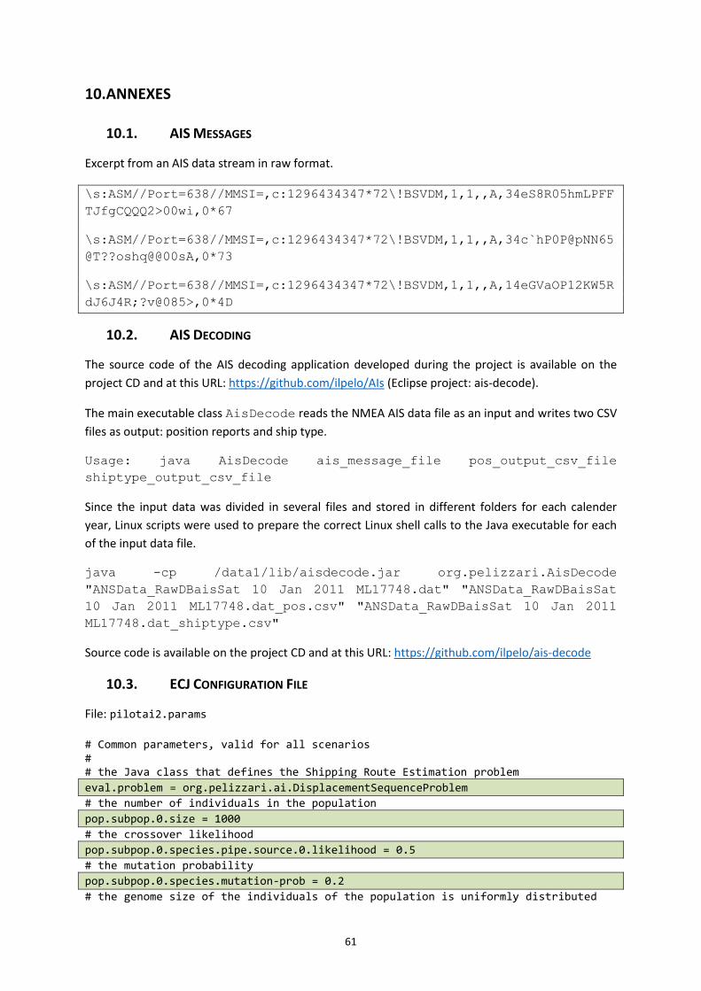
61
10. ANNEXES
10.1. AIS MESSAGES
Excerpt from an AIS data stream in raw format.
\s:ASM//Port=638//MMSI=,c:1296434347*72\!BSVDM,1,1,,A,34eS8R05hmLPFF
TJfgCQQQ2>00wi,0*67
\s:ASM//Port=638//MMSI=,c:1296434347*72\!BSVDM,1,1,,A,34c`hP0P@pNN65
@T??oshq@@00sA,0*73
\s:ASM//Port=638//MMSI=,c:1296434347*72\!BSVDM,1,1,,A,14eGVaOP12KW5R
dJ6J4R;?v@085>,0*4D
10.2. AIS DECODING
The source code of the AIS decoding application developed during the project is available on the
project CD and at this URL: https://github.com/ilpelo/AIs (Eclipse project: ais-decode).
The main executable class AisDecode reads the NMEA AIS data file as an input and writes two CSV
files as output: position reports and ship type.
Usage: java AisDecode ais_message_file pos_output_csv_file
shiptype_output_csv_file
Since the input data was divided in several files and stored in different folders for each calender
year, Linux scripts were used to prepare the correct Linux shell calls to the Java executable for each
of the input data file.
java -cp /data1/lib/aisdecode.jar org.pelizzari.AisDecode
"ANSData_RawDBaisSat 10 Jan 2011 ML17748.dat" "ANSData_RawDBaisSat
10 Jan 2011 ML17748.dat_pos.csv" "ANSData_RawDBaisSat 10 Jan 2011
ML17748.dat_shiptype.csv"
Source code is available on the project CD and at this URL: https://github.com/ilpelo/ais-decode
10.3. ECJ CONFIGURATION FILE
File: pilotai2.params # Common parameters, valid for all scenarios # # the Java class that defines the Shipping Route Estimation problem
eval.problem = org.pelizzari.ai.DisplacementSequenceProblem
# the number of individuals in the population
pop.subpop.0.size = 1000
# the crossover likelihood
pop.subpop.0.species.pipe.source.0.likelihood = 0.5
# the mutation probability
pop.subpop.0.species.mutation-prob = 0.2
# the genome size of the individuals of the population is uniformly distributed
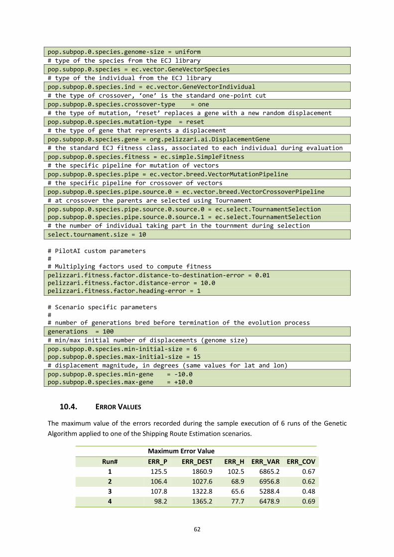
62
pop.subpop.0.species.genome-size = uniform
# type of the species from the ECJ library
pop.subpop.0.species = ec.vector.GeneVectorSpecies
# type of the individual from the ECJ library
pop.subpop.0.species.ind = ec.vector.GeneVectorIndividual
# the type of crossover, ‘one’ is the standard one-point cut
pop.subpop.0.species.crossover-type = one
# the type of mutation, ‘reset’ replaces a gene with a new random displacement
pop.subpop.0.species.mutation-type = reset
# the type of gene that represents a displacement
pop.subpop.0.species.gene = org.pelizzari.ai.DisplacementGene
# the standard ECJ fitness class, associated to each individual during evaluation
pop.subpop.0.species.fitness = ec.simple.SimpleFitness
# the specific pipeline for mutation of vectors
pop.subpop.0.species.pipe = ec.vector.breed.VectorMutationPipeline
# the specific pipeline for crossover of vectors
pop.subpop.0.species.pipe.source.0 = ec.vector.breed.VectorCrossoverPipeline
# at crossover the parents are selected using Tournament
pop.subpop.0.species.pipe.source.0.source.0 = ec.select.TournamentSelection pop.subpop.0.species.pipe.source.0.source.1 = ec.select.TournamentSelection
# the number of individual taking part in the tournment during selection
select.tournament.size = 10
# PilotAI custom parameters # # Multiplying factors used to compute fitness
pelizzari.fitness.factor.distance-to-destination-error = 0.01 pelizzari.fitness.factor.distance-error = 10.0 pelizzari.fitness.factor.heading-error = 1
# Scenario specific parameters # # number of generations bred before termination of the evolution process
generations = 100
# min/max initial number of displacements (genome size)
pop.subpop.0.species.min-initial-size = 6 pop.subpop.0.species.max-initial-size = 15
# displacement magnitude, in degrees (same values for lat and lon)
pop.subpop.0.species.min-gene = -10.0 pop.subpop.0.species.max-gene = +10.0
10.4. ERROR VALUES
The maximum value of the errors recorded during the sample execution of 6 runs of the Genetic
Algorithm applied to one of the Shipping Route Estimation scenarios.
Maximum Error Value
Run# ERR_P ERR_DEST ERR_H ERR_VAR ERR_COV
1 125.5 1860.9 102.5 6865.2 0.67
2 106.4 1027.6 68.9 6956.8 0.62
3 107.8 1322.8 65.6 5288.4 0.48
4 98.2 1365.2 77.7 6478.9 0.69
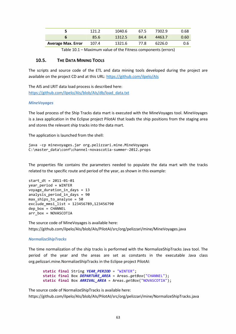
63
5 121.2 1040.6 67.5 7302.9 0.68
6 85.6 1312.5 84.4 4463.7 0.60
Average Max. Error 107.4 1321.6 77.8 6226.0 0.6
Table 10.1 – Maximum value of the Fitness components (errors)
10.5. THE DATA MINING TOOLS
The scripts and source code of the ETL and data mining tools developed during the project are
available on the project CD and at this URL: https://github.com/ilpelo/AIs
The AIS and LRIT data load process is described here:
https://github.com/ilpelo/AIs/blob/AIs/db/load_data.txt
MineVoyages
The load process of the Ship Tracks data mart is executed with the MineVoyages tool. MineVoyages
is a Java application in the Eclipse project PilotAI that loads the ship positions from the staging area
and stores the relevant ship tracks into the data mart.
The application is launched from the shell:
java -cp minevoyages.jar org.pelizzari.mine.MineVoyages C:\master_data\conf\channel-novascotia-summer-2012.props
The properties file contains the parameters needed to populate the data mart with the tracks
related to the specific route and period of the year, as shown in this example:
start_dt = 2011-01-01 year_period = WINTER voyage_duration_in_days = 13 analysis_period_in_days = 90 max_ships_to_analyse = 50 exclude_mmsi_list = 123456789,123456790 dep_box = CHANNEL arr_box = NOVASCOTIA
The source code of MineVoyages is available here:
https://github.com/ilpelo/AIs/blob/AIs/PilotAI/src/org/pelizzari/mine/MineVoyages.java
NormalizeShipTracks
The time normalization of the ship tracks is performed with the NormalizeShipTracks Java tool. The
period of the year and the areas are set as constants in the executable Java class
org.pelizzari.mine.NormalizeShipTracks in the Eclipse project PilotAI:
static final String YEAR_PERIOD = "WINTER"; static final Box DEPARTURE_AREA = Areas.getBox("CHANNEL"); static final Box ARRIVAL_AREA = Areas.getBox("NOVASCOTIA");
The source code of NormalizeShipTracks is available here:
https://github.com/ilpelo/AIs/blob/AIs/PilotAI/src/org/pelizzari/mine/NormalizeShipTracks.java

64
10.6. SHIPPING ROUTE ESTIMATION TOOL
The Machine Learning software is available on the project CD and at this URL:
https://github.com/ilpelo/AIs. The software can be built on the Eclipse IDE using the projects: PilotAI
and TrackGIS. The external libraries are: ecj.22.jar and minigeo-r6.jar.
The Shipping Route Estimation Tool is configured by setting the following constants in the Java class
org.pelizzari.ai.DisplacementSequenceProblem in the Eclipse project PilotAI:
static final String YEAR_PERIOD = "WINTER"; static final Box DEPARTURE_AREA = Areas.getBox("REDSEA"); static final Box ARRIVAL_AREA = Areas.getBox("GOA");
The tool starts by calling the ECJ executable class ec.Evolve with the parameter: -file
pilotai2.params (see Section 10.3). The output is saved in the database (table fitness) and in the
local directory C:\master_data. Several KML files are created and are used to visualize the training
set and the resulting routes throughout the evolutionary process.