D-4474-1 1

Generic Structures:

First-Order Positive Feedback

Produced for the

System Dynamics in Education Project

MIT System Dynamics Group

Under the Supervision of

Dr. Jay W. Forrester

Sloan School of Management

Massachusetts Institute of Technology

by

Stephanie Albin

Mark Choudhari

March 8, 1996

Vensim Examples added October 2001

Copyright © 2001 by the Massachusetts Institute of Technology

Permission granted to copy for non-commercial educational purposes

6

4 D-4474-2

Table of Contents

1. INTRODUCTION 5

2. EXPONENTIAL GROWTH

2.1. EXAMPLE 1: POPULATION-BIRTH SYSTEM 7

2.2. EXAMPLE 2: BANK BALANCE-INTEREST SYSTEM 7

2.3. EXAMPLE 3: KNOWLEDGE-LEARNING SYSTEM 8

3. THE GENERIC STRUCTURE 8

3.1. MODEL DIAGRAM 9

3.2. MODEL EQUATIONS 9

3.3. MODEL BEHAVIOR 11

4. BEHAVIORS PRODUCED BY THE GENERIC STRUCTURE 12

5. SUMMARY OF IMPORTANT CHARACTERISTICS

6. USING INSIGHTS GAINED FROM THE GENERIC STRUCTURE

6.1. EXERCISE 1: SOFTWARE SALES 16

6.2. EXERCISE 2: MAKING FRIENDS 17

6.3. EXERCISE 3: ACCOUNT BALANCE 18

7. SOLUTIONS TO EXERCISES 18

8. APPENDIX - MODEL DOCUMENTATION

9. VENSIM EXAMPLES

14

15

20

22

D-4474-2 5 5

1. Introduction

Generic structures are relatively simple structures that recur in many diverse

situations. In this paper, for example, the models of a bank account and a deer population

are shown to share the same basic structure! Transferability of structure between systems

gives the study of generic structures its importance in system dynamics.

Road Maps contains a series of papers on generic structures. In these papers, we

will study generic structures to develop our understanding of the relationship between the

structure and behavior of a system. Such an understanding should help us refine our

intuition about the systems that surround us and allow us to improve our ability to model

the behaviors of systems.

We can transfer knowledge about a generic structure in one system to understand

the behavior of other systems that contain the same structure. Our knowledge of generic

structures and the behaviors they produce is transferable to systems we have never studied

before!

It is often the case that the behavior of a system is more obvious than its

underlying structure. Systems are then referred to by the common behaviors they

produce. However, it is incorrect to assume such systems are capable of exhibiting only

their most popular behaviors, and we need to look more closely at the other behaviors

possible. In effect, our study of generic structures examines the range of behaviors

possible from particular structures. In each case, we seek to understand what in the

structure is responsible for the behavior produced.

This paper introduces a simple generic structure of first-order linear positive

feedback. We illustrate our study of the positive feedback structure with many examples

of systems containing the structure. You will soon begin to recognize the structure in

many of the models you see and build. In the exercises at the end of the paper, we provide

you with an opportunity to see how you can transfer your knowledge between different

systems.

D-4474-2 6

2. Exponential Growth

Exponential growth is produced by a positive feedback loop between the

components of a system. The characteristic behavior of exponential or compound growth

is shown in Figure 1. Many systems in the world exhibit the exponential behavior of a

process feeding upon itself. For example, in an ecological system, the birth of deer

increases the deer population, which further increases the number of deer that are born.

At your bank, your account balance is increased by the interest you earn on it, and the

larger your balance gets, the more interest you earn on it! Another system which can be

said to exhibit exponential growth is the knowledge-learning system. Simply stated, the

more you know, the faster you learn, and then gain even more knowledge. 1: STOCK

2000.00

1050.00

100.00 0.00 3.00 6.00 9.00 12.00

Time

1 1

1

1

Figure 1 Exponential Growth Curve

These very different systems exhibit the same behavior pattern because the relationship

between their components is fundamentally the same. They all contain the first-order

linear positive feedback generic structure. Population is related to births in the same way

your bank balance is related to the interest it earns and knowledge is related to learning.

Let us begin to explore the nature of this relationship by looking at the structure of

our three example systems.

D-4474-2 7 7

2.1. Example 1: Population-Birth system

Our first example shown in figure 2 is taken from the ecology of a deer population.

The deer population is the stock, and the births of deer is the net inflow to the stock.

The amount of deer births is equal to the amount of female deer that reproduce and is

calculated as a compounding fraction (called birth fraction) of the total deer population.

The

births = deer population * birth fraction.

deer population births

birth fraction

Figure 2 Model of a population-birth system

2.2. Example 2: Bank balance-interest system

Our second example in figure 3 shows the relationship between a bank balance and

the interest it earns. The bank balance is the stock, and the interest earned is the inflow

to the stock. The amount of interest earned every year is equal to a compounding fraction

(interest rate) of the bank balance. The

interest earned = bank balance * interest rate.

bank balance interest earned

interest rate

Figure 3 Model of a bank balance system

D-4474-2 8

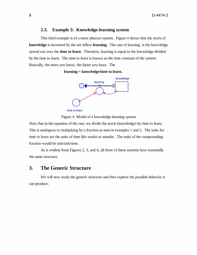
2.3. Example 3: Knowledge-learning system

This third example is of a more abstract system. Figure 4 shows that the stock of

knowledge is increased by the net inflow learning. The rate of learning is the knowledge

spread out over the time to learn. Therefore, learning is equal to the knowledge divided

by the time to learn. The time to learn is known as the time constant of the system.

Basically, the more you know, the faster you learn. The

learning = knowledge/time to learn.

knowledge learning

time to learn

Figure 4 Model of a knowledge-learning system

Note that in the equation of the rate, we divide the stock (knowledge) by time to learn.

This is analogous to multiplying by a fraction as seen in examples 1 and 2. The units for

time to learn are the units of time like weeks or months. The units of the compounding

fraction would be unit/unit/time.

As is evident from Figures 2, 3, and 4, all three of these systems have essentially

the same structure.

3. The Generic Structure

We will now study the generic structure and then explore the possible behavior it

can produce.

D-4474-2 9 9

3.1. Model Diagram

stock flow

compounding fraction or time constant

Figure 5 Model of the underlying generic structure

The model diagram of the first-order positive generic structure is shown in figure 5. In the

equation of the rate, we multiply the stock by the compounding fraction or divide the

stock by the time constant. The time constant is simply the reciprocal of the compounding

fraction.

3.2. Model Equations

The equations for the generic structure are

stock(t) = stock(t - dt) + (flow) * dt

DOCUMENT: This is the stock of the system. It corresponds to the deer population, the

bank balance, and the stock of knowledge in the examples above.

UNIT: units

INFLOWS:

flow = stock*compounding_fraction

DOCUMENT: The flow is the fraction of the stock that flows into the system per unit

time. It corresponds to the births, the interest earned, and the learning in the examples

above.

UNIT: units/time

compounding_fraction = a constant

10 D-4474-2

DOCUMENT: This is the compounding fraction or growth factor. It determines the

inflow to the stock. The compounding fraction corresponds to the birth fraction and the

interest rate in the examples above. It is the amount of units added to the stock for every

unit already in the stock, every time.

UNIT: units/unit/time

Note: If we had a time constant instead of a compounding fraction the equation for the

flow and the time constant would be

INFLOWS:

flow = stock/time constant

UNIT: units/time

D-4474-2 1111

time_constant = a constant

DOCUMENT: This is the time constant. It is the adjustment time for the stock. It

corresponds to the time to learn in the above example. This is the time for each initial unit

to compound into a new unit.

UNIT: time

From the comparison of the two possible equations for the rate, we notice that the

multiplier in the rate equation is given by

1multiplier (for the stock) in the rate equation = compounding fraction =

time constant

3.3. Model Behavior

The characteristic feature of exponential growth is its constant doubling time, i.e.

the time it takes for the stock to double remains constant. For example in Figure 6, it

takes the stock 7 years to double from 100 to 200 and also the same time to double from

800 to 1600! 1: STOCK 2: FLOW 3: COMPOUNDING FRACTION

1: 1600.00 2: 3: 1.10

1: 800.002: 3: 0.10

1: 2: 0.00 3: -0.90

0.00 7.00 14.00 21.00 28.00 Time

1

1

1

1

2 2 2 2

3 3 3 3

Figure 6 Results of a simulation of the positive feedback generic structure.

To find the doubling time of the stock, we need the time constant of the system. The time

constant may either be given to you directly (as the time to learn in Example 3 above), or

12 D-4474-2

if you have a compounding fraction, the time constant is simply it’s reciprocal. The time

constant is obtained from the compounding fraction by

1Time constant =

compounding fraction

The doubling time for the stock is given by

Doubling time ? 0.7 ? Time constant 1

4. Behaviors produced by the generic structure

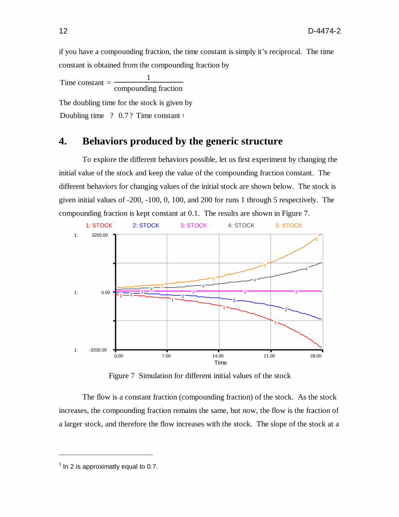
To explore the different behaviors possible, let us first experiment by changing the

initial value of the stock and keep the value of the compounding fraction constant. The

different behaviors for changing values of the initial stock are shown below. The stock is

given initial values of -200, -100, 0, 100, and 200 for runs 1 through 5 respectively. The

compounding fraction is kept constant at 0.1. The results are shown in Figure 7. 1: STOCK 2: STOCK 3: STOCK 4: STOCK 5: STOCK

1: 3200.00

1: 0.00

1: -3200.00 0.00 7.00 14.00 21.00 28.00

Time

1 1

1

1

2 2 2

2

3 3 3 34 4

4

4

5 5

5

5

Figure 7 Simulation for different initial values of the stock

The flow is a constant fraction (compounding fraction) of the stock. As the stock

increases, the compounding fraction remains the same, but now, the flow is the fraction of

a larger stock, and therefore the flow increases with the stock. The slope of the stock at a

1 ln 2 is approximatly equal to 0.7.

D-4474-2 1313

point in time is equal to the net flow into it at that time. Therefore, for each curve, the

slope of the stock is increasing or decreasing as the stock is increasing or decreasing.

With a positive value for the compounding fraction, the nature of the behavior is

determined by whether the initial value of the stock is positive or negative. For the loop

to be a positive feedback loop, we require that the compounding fraction be positive2.

Therefore, we see that the generic structure of a first-order positive loop can

exhibit three types of behavior - positive exponential growth, unstable3 equilibrium, and

negative exponential growth.

Let us now explore what accelerates or retards the exponential growth of a

system. We will study the effect of changing the value of the compounding fraction while

keeping the initial value of the stock constant. The compounding fraction is given values

of 0, 0.1, 0.2, 0.3, and 0.4 for runs 1 through 5 respectively. The initial value of the stock

is kept constant at 100. The change in rate of exponential growth is shown in Figure 8. 1: STOCK 2: STOCK 3: STOCK 4: STOCK 5: STOCK

1: 5000.00

1: 2500.00

1: 0.00 0.00 7.00 14.00 21.00 28.00

Time

1 1 1 12 2 2

2

3

3

3

4

4

5

Figure 8 Simulation for different values of the compounding fraction

2 A positive compounding fraction is required for a positive feedback (reinforcing) loop as it gives the net flow the sign of the stock (either positive or negative). A negative value for the compounding fraction will make the loop a negative feedback or balancing loop. 3 This equilibrium is called unstable as the slightest deviation of the value of the stock away from zero will destroy the equilibrium and result in exponential growth.

14 D-4474-2

The slope of the stock at a specific point4 in time is equal to the net flow into it at

that time. The flow is a larger fraction of the stock for a larger compounding fraction.

Therefore, the slope of the stock is greater for a larger compounding fraction.

The larger the compounding fraction is, the larger the flow and the faster the

growth of the stock. A larger compounding fraction accelerates exponential growth.

For a negative initial value of the stock, the effect of the compounding fraction on

growth rate is the same, except the growth is in the negative direction.

5. Summary of important characteristics

Structure:

The loop is a positive feedback loop if and only if the stock has a positive sign in

the equation for net flow into the stock. A positive sign in the equation for flow gives the

flow the same sign as the stock (reinforcing behavior). Therefore, the simplest positive

feedback loop requires a positive compounding fraction for the inflow to the stock.

Behavior:

We summarize the behavior of the positive feedback loop in table 1 below.

Although positive feedback loops are best known for their exponential growth, they do

exhibit other behaviors. Remember: A negative multiplier in the rate does not create a

positive feedback loop.

The generic structure of a first-order positive loop can exhibit three types of

behavior - positive exponential growth, unstable equilibrium, and negative exponential

growth.

For an initial value of the stock and

the multiplier in the rate (fraction or

time constant), Stock

the behavior of the stock is given in

italics Negative Zero Positive

4 The slope of the stock at a point is the slope of the line tangent to the curve at that point.

D-4474-2 1515

Compounding

Zero Equilibrium Zero Equilibrium

Fraction5

Positive Negative

Exponential

growth

Zero Positive

Exponential

growth

Table 1 Summary of the behavior of a positive feedback loop

Exponential growth requires an initial value of the stock other than zero. Exponential

growth has a constant doubling time. The rate at which an exponential growth occurs

increases with the value of the compounding fraction.

Look over table 1 and the graphs of the simulation runs till you internalize your

knowledge about positive feedback loops. When you feel confident about your

understanding of the behavior, you should go on to the exercises in the next section.

6. Using insights gained from the generic structure

We have seen examples of different systems with the same positive feedback loop

structure. We studied the underlying generic structure to develop our intuition about

positive loops. Now, we apply the insight we gained from the generic structure to

understand the behavior of other systems.

To do the exercises below, you need not simulate the models; hand computation

should suffice. However, after answering the questions we encourage you to build and

experiment with the models.

5 Zero compounding fraction corresponds to an infinite time constant. This is not a situation you

will be confronted with.

16 D-4474-2

6.1. Exercise 1: Software sales

The customer base of a software manufacturer increases with the addition of new

customers. Through the word of mouth, a fraction of the present customers encourage

other people to become new customers. The model for this simple positive feedback

system is shown below.

customer base new customers

fractional increase of customers

Figure 10 Model for Software sales

There are two software companies, Nanosoft and Picosoft, each of which have a customer

base consisting of 10,000 customers, and a fractional increase is 0.1

customers/customer/week (the fraction means that 1 out of 10 customers convinces

another person to become a customer each week).

1. What is the time constant and doubling time? Give their units. What are the units of

new customers?

2. Approximately how much time does it take for the customer base of Nanosoft to grow

to 40,000 customers?

3. If Nanosoft wants to have 80,000 customers in the same amount of time, how could it

change the initial value of the stock to achieve this?6

4. Picosoft also wants 80,000 customers in the same time but decides to change the

fractional increase to achieve this. What change should it make?

5. If Nanosoft has a customer base three times larger than Picosoft, which of the two

firms do you think will grow faster? What is the ratio of their customer bases after 14

weeks?

Although changing the initial stock may not be a feasible option in the real system, our purpose here is to understand the effect of different initial values of the stock on its growth.

6

D-4474-2 1717

6.2. Exercise 2: Making Friends

Brenda and Brandon are twins who have just moved into a new town to live with

their aunt. Although they are twins, their personalities are quite different. Brenda is very

sociable and makes friends easily. She usually makes a new friend, though each friend she

already has, every 2 weeks. Brandon, on the other hand, is quite shy; it usually takes him

twice as long as Brenda to make a new friend through each of his current friends.

In this new town, Brandon already has 5 friends that he made in previous summer

visits. Brenda, however, has never been to this town before and the only ‘friend’she has

here is her aunt.

Figure 11 is a very simple model of the process by which new friends are made.

The model indicates that the rate at which a person makes new friends depends on the

amount of friends that a person already has and the time to make a new friend. For

example, if Brenda has a lot of friends, she will be introduced to a lot of new people

(friends of friends), and if she doesn’t take much time to make friends with a new person,

then she will make a lot of new friends very quickly.

number of friends

Making new friends

time to make a new friend

Figure 11 Model for making friends

1. What is the time constant and doubling time for Brenda?

2. What is the time constant and doubling time for Brandon?

3. By the time school starts (9 weeks after moving in) who will have more friends,

Brenda or Brandon? You don’t need to find exactly how many friends Brenda and

Brandon have after 9 weeks; just provide an indication of who has more friends after 9

weeks.

18 D-4474-2

6.3. Exercise 3: Account balance

Brandon decides he has had enough of school, and plans to start his own software

business to compete with Nanosoft and Picosoft. We have built a model of his account

balance shown in figure 12. A loan is considered as a negative account balance.

account balance interest payments

interest rate for borrowing

Figure 12 Model for account balance

To buy a computer, he takes out a $2,000 loan from his bank at an interest rate of 5%.

On his way home from the bank, he meets Brenda who tells him of another bank that will

forgive $1,000 of his loan if he transfers to them. This bank charges an interest rate of

10%. Brandon doesn’t understand exponential growth very well and is confused about

what he should do. What do you recommend? What will his account balance be after 14

years for each bank?

7. Solutions to Exercises

7.1. Answer to Section 6.1: Software Sales 1

1. The time constant = , or 10 weeks.fractional increase

The doubling time = 0.7 x the time constant, or 7 weeks.

2. For the customer base of 10,000 to grow to 40,000, the initial base doubles twice.

Each doubling time is 7 weeks, thus it takes 14 weeks for the firm to reach 40,000

customers.

3. Since the time to reach 80,000 is given as 14 weeks (two doubling times), the initial

value for the stock should be 20,000 customers.

4. To reach 80,000 customers, a base of 10,000 doubles three times in the 14 weeks.

Working backwards:

D-4474-2 1919

141 doubling time = or 4. 6 weeks.

3

doubling time1 time constant = = 6.6 weeks.

0.7 1 21

Fractional increase = = or .15 customers/cust/weektime constant 140

5. Nanosoft grows faster since it has a larger stock than Picosoft. While the fractional

increase of each company is the same, the rate of growth for Nanosoft is larger because

the actual number of customers the fractional increase corresponds to is larger. The ratio

of customer bases after 14 weeks is still the same, 3 to 1. It may seem impossible for the

ratio to remain the same while one firm grows at a faster rate than the other. The key to

understand is that Nanosoft does grow faster but also has a larger distance to go to

maintain the ratio of 3 to 1.

7.2. Answer to Section 6.2: Making Friends 1. Brenda’s time constant is her time to make a new friend, which equals 2 weeks. The

doubling time is the time constant x 0.7, or 1.4 weeks.

2. Brandon takes twice as long to make friends. His time to make a new friend is twice

that of Brenda’s. His time constant is thus 4 weeks. The doubling time is the time

constant x 0.7, or 2.8 weeks.

3. The easiest way to answer this question is to use the doubling times and the initial

values for the stocks of friends and make a small chart of Brenda and Brandon’s number

of friends for the summer.

Week Brenda’s Friends Brandon’s Friends

0 1 5

1.4 2 —

2.8 4 10

4.2 8 —

5.6 16 20

7.0 32 —

8.4 64 40

20 D-4474-2

9 more than Brandon less than Brenda

Because of the nature of the positive generic structure, once Brenda has more friends that

Brandon, she will always have more friends that Brandon. We can then infer that in week

9, the end of the summer, Brenda has more friends than Brandon.

7.3. Answer to Section 6.3: Account Balance Brandon’s bank’s interest rate is 0.05. The time constant is equal to 20, and the

doubling time of the debt is equal to 14 years. The other bank’s interest rate is 0.1 and

has a time constant of 10 years. The doubling time of a debt is 7 years.

Years Debt in Brandon’s Bank Debt in Other Bank

0 2000 1000

14 4000 4000

28 8000 16000

42 16000 64000

56 32000 256000

This chart clearly illustrates the power of exponential growth. The bank which

Brandon should invest in depends on when he plans on paying back his loan. If he plans

to pay back in the first 14 years, then the other bank would save him money. If it will take

Brandon over 14 years to repay the loan, the bank he already borrowed from is his best

bet.

8. Appendix - Model Documentation

8.1. Documentation for section 2.1: Population-birth system

deer population(t) = deer population(t - dt) + (births) * dt

INIT deer population = 100

DOCUMENT: This is the number of deer present in the system.

UNIT: deer

INFLOWS:

D-4474-2 2121

births = deer population * birth fraction

DOCUMENT:This is the number of deer born every year.

UNIT: deer/year

birth fraction = .3

DOCUMENT: This is the number of deer born per deer every year.

UNIT: deer/deer/year

8.2. Documentation for section 2.2: Bank balance-interest system

bank balance(t) = bank balance(t - dt) + (interest earned) * dt

INIT bank balance = 100

DOCUMENT: This is the amount of money in a bank account

UNIT: dollars

INFLOWS:

interest earned = bank balance * interest rate

DOCUMENT: This is the amount of interest earned per year on the money in the

account.

UNIT: dollars/year

interest rate = .025

DOCUMENT: This is the number of dollars earned per dollar in 1 year.

UNIT: dollars/dollar/year

8.3. Documentation for section 2.3: Knowledge-learning system

knowledge(t) = knowledge(t - dt) + (learning) * dt

INIT knowledge = 100

22 D-4474-2

DOCUMENT: This is the amount a person knows, measured in facts about a subject.

UNIT: facts

INFLOWS:

learning = knowledge /time to learn

DOCUMENT: This is the rate at which new facts are learned per day.

UNIT: facts/day

time to learn = 3

DOCUMENT: This is the time constant of the system. It takes an average of 3 days for

each fact to assist in the learning of a new fact.

UNIT: day

D-4474-2 2323

Vensim Examples:Generic Structures: First-Order Linear Positive

FeedbackBy Aaron Diamond

October 2001

2.1 Example 1: Population-Birth system

Deer Populationbirths

BIRTH FRACTION

INITIAL DEER POPULATION

Figure 13: Vensim Equivalent of Figure 2: Model of a population-birth system

Documentation for population-birth model

(1) BIRTH FRACTION=0.3 Units: deer/deer/year This is the number of deer born per deer every year.

(2) births=Deer Population*BIRTH FRACTION Units: deer/year The flow is the number of deer born every year.

(3) Deer Population= INTEG (births, INITIAL DEER POPULATION) Units: deer This is the number of deer present in the system.

(4) INITIAL DEER POPULATION=100 Units: deer

(5) FINAL TIME = 28

24 D-4474-2

Units: year The final time for the simulation.

(6) INITIAL TIME = 0 Units: year The initial time for the simulation.

(7) SAVEPER = TIME STEP Units: year The frequency with which output is stored.

(8) TIME STEP = 0.0625 Units: year The time step for the simulation.

D-4474-2 2525

2.2 Example 2: Bank balance-interest system

Bank Balance interest earned

INTEREST RATE INITIAL BANK BALANCE

Figure 14: Vensim Equivalent of Figure 3: Model of a bank balance system

Documentation for bank balance model

(1) Bank Balance= INTEG (interest earned, INITIAL BANK BALANCE) Units: dollars This is the amount of money in a bank account.

(2) FINAL TIME = 28 Units: year The final time for the simulation.

(3) INITIAL BANK BALANCE=100 Units: dollars

(4) INITIAL TIME = 0 Units: year The initial time for the simulation.

(5) interest earned=Bank Balance*INTEREST RATE Units: dollars/year The flow is the amount of interest earned per year on the money in the account.

(6) INTEREST RATE=0.025 Units: dollars/dollars/year This is the number of dollars earned per dollar in 1 year.

26 D-4474-2

(7) SAVEPER =TIME STEP Units: year The frequency with which output is stored.

(8) TIME STEP = 0.0625 Units: year The time step for the simulation.

2.3 Example 3: Knowledge-learning system

Knowledge

learning

TIME TO LEARN INITIAL KNOWLEDGE

Figure 15: Vensim Equivalent of Figure 4: Model of a knowledge-learning system

Documentation for knowledge-learning model

(1) FINAL TIME = 28 Units: day The final time for the simulation.

(2) INITIAL KNOWLEDGE=100 Units: facts

(3) INITIAL TIME = 0 Units: day The initial time for the simulation.

(4) Knowledge= INTEG (learning, INITIAL KNOWLEDGE)

D-4474-2 2727

Units: facts

This is the amount a person knows, measured in facts about a

subject.

(5) learning=Knowledge/TIME TO LEARN Units: facts/day This is the rate at which new facts are learned per day.

(6) SAVEPER =TIME STEP Units: day The frequency with which output is stored.

(7) TIME STEP = 0.0625 Units: day The time step for the simulation.

(8) TIME TO LEARN=3 Units: day This is the time constant of the system. It takes an average of 3 days for each fact to assist in the learning of a new fact.

28 D-4474-2

3.1. Model Diagram

Stock flow

COMPOUNDING FRACTION or TIME CONSTANT

INITIAL STOCK

Figure 16: Vensim Equivalent of Figure 5: Model of the underlying generic structure

Documentation for generic structure model

(1) COMPOUNDING FRACTION or TIME CONSTANT=a constant Units: units/units/time for COMPOUNDING FRACTION, Units: time for TIME CONSTANT This is the compounding fraction or growth factor. It determines the inflow to the stock. The compounding fraction corresponds to the birth fraction and the interest rate in the examples above. It is the amount of units added to the stock for every unit already in the stock, every time.

(2) FINAL TIME =28 Units: Month The final time for the simulation.

(3) flow=Stock*COMPOUNDING FRACTION, or Stock/TIME CONSTANT Units: units/time The flow is the fraction of the stock that flows into the system per unit time. It corresponds to the births, the interest earned, and the learning in the examples above.

(4) INITIAL STOCK=a constant Units: units

D-4474-2 2929

(5) INITIAL TIME = 0 Units: Month The initial time for the simulation.

(6) SAVEPER =TIME STEP Units: Month The frequency with which output is stored.

(7) Stock= INTEG (flow, INITIAL STOCK) Units: units This is the stock of the system. It corresponds to the deer population, the bank balance, and the stock of knowledge in the examples above.

(8) TIME STEP = .0625 Units: Month The time step for the simulation.

Graph of Stock, flow and COMPOUNDING FRACTION 1600 units

1600 units/time

1.1 1/time

0 units

0 units/time

-0.9 1/time

1

3 3 3 1

1

3

1 1

21

2 1 1

2 2

1 1

2 2 2 2 2 2

3

0 4 8 12 16 20 24 28 Time (time)

Stock : 1 1 1 1 1 1 1 1 1 units flow : 2 2 2 2 2 2 2 2 units/time COMPOUNDING FRACTION : 3 3 3 3 3 1/time

Figure 17: Vensim equivalent of Figure 6: Results of a simulation of the positive feedback generic structure.

5

30 D-4474-2

Graph of Stock with Different Initial Values

3,200

-3,2000 4 8 12 16 20 24 28

Time (Month)

Stock : Stock(0)=-200 1 1 1 1 1 1 units Stock : Stock(0)=-100 2 2 2 2 2 2 2 units Stock : Stock(0)=0 3 3 3 3 3 3 3units Stock : Stock(0)=100 4 4 4 4 4 4 unitsStock : Stock(0)=200 5 5 5 5 5 5 units

Figure 18: Vensim Equivalent of Figure 7: Simulation for different initial values of the Stock

Graph of Stock with Different Values of the COMPOUNDING FRACTION

5

543 543

543

5 4

3

5 4

3

4

3

4

321 21 21 21 2

1 2 21

1

5,000

10 0 4 8 12 16 20 24 28

Time (Month)

Stock : CF=0 1 1 1 1 1 1 1 units Stock : CF=0.1 2 2 2 2 2 2 2 units Stock : CF=0.2 3 3 3 3 3 3 3 units Stock : CF=0.3 4 4 4 4 4 4 4 units Stock : CF=0.4 5 5 5 5 5 5 5 units

4

3

5

3

321 54 321

4

1 3

2 1 2 1 2

1

2

1

2

Figure 19: Vensim Equivalent of Figure 8: Simulation for different values of the

COMPOUNDING FRACTION