Generative Modeling with Conditional Autoencoders:Building an Integrated Cell

Gregory R. Johnson gregj@alleninstitute.orgRory M. Donovan-Maiye rorydm@alleninstitute.orgMary M. Maleckar mollym@alleninstitute.orgAllen Institute for Cell Science, 615 Westlake Ave N, Seattle, WA 98109

AbstractWe present a conditional generative model tolearn variation in cell and nuclear morphologyand the location of subcellular structures frommicroscopy images. Our model generalizes to awide range of subcellular localization and allowsfor a probabilistic interpretation of cell and nu-clear morphology and structure localization fromfluorescence images. We demonstrate the ef-fectiveness of our approach by producing photo-realistic cell images using our generative model.The conditional nature of the model provides theability to predict the localization of unobservedstructures given cell and nuclear morphology.

1. IntroductionA central biological principle is that cellular organization isstrongly related to function. Location proteomics (Murphy,2005) addresses this by aiming to determine cell state – i.e.subcellular organization – by elucidating the localization ofall structures and how they change through the cell cycle,and in response to perturbations, e.g., mutation. However,determining cellular organization is challenged by the mul-titude of different molecular complexes and organelles thatcomprise living cells and drive their behaviors (Kim et al.,2014). Currently, the experimental state-of-the-art for livecell imaging is limited to the simultaneous visualization ofonly a limited number of tagged (2-6 tagged) molecules.Modeling approaches can address this limitation by inte-grating subcellular structure data from diverse imaging ex-periments. Due to the number and diversity of subcellularstructures, it is necessary to build models that generalizewell with respect to both representation and interpretation.

Image feature-based methods have previously been em-

Preprint

ployed to describe and model cell organization (Boland &Murphy, 2001; Carpenter et al., 2006; Rajaram et al., 2012).While useful for discriminative tasks, these approaches donot explicitly model the relationships between subcellularcomponents, limiting the application to integration of all ofthese structures.

Generative models are useful in this context. They cap-ture variation in a population and encode it as a probabilitydistribution, accounting for the relationships among struc-tures. Fundamental work has previously demonstrated theutility of expressing subcellular structure patterns as a gen-erative model, which can then be used as a building blockfor models of cell behavior, i.e. (Murphy, 2005; Donovanet al., 2016).

Ongoing efforts to construct generative models of cell or-ganization are primarily associated with the CellOrganizerproject (Zhao & Murphy, 2007; Peng & Murphy, 2011).That work implements a “cytometric” approach to mod-eling that considers the number of objects, lengths, sizes,etc. from segmented images and/or inverse procedural mod-eling, which can be particularly useful for both analyzingimage content and approaching integrated cell organiza-tion. These methods support parametric modeling of manysubcellular structure types and, as such, generalize wellwhen low amounts of appropriate imaging data are avail-able. However, these models may depend on preprocessingmethods, such as segmentation, or other object identifica-tion tasks for which a ground truth is not available. Ad-ditionally, there may exist subcellular structures for whicha parametric model does not exist or may not be appropri-ate e.g., structures that vary widely in localization (diffuseproteins), or reorganize dramatically during e.g. mitosis orduring a stimulated state (such as microtubules).

Thus, the presence of key structures for which current meth-ods are notwell suitedmotivates the need for a newapproachthat generalizes well to a wide range of structure localiza-tion.

Recent advances in adversarial networks (Goodfellow et al.,

arX

iv:1

705.

0009

2v1

[st

at.M

L]

28

Apr

201

7

Building the Integrated Cell

2014) are relevant to our problem. They have the abilityto learn distributions over images, generate photo-realisticexemplars, and learn sophisticated conditional relation-ships; see e.g. Generative Adversarial Networks (Good-fellow et al., 2014), Varational Autoencoders/GAN (Larsenet al., 2015), Adversarial Autoencoders (Makhzani et al.,2015).

Leveraging these recent advances, we present a non-parametric model of cell shape and nuclear shape and lo-cation, and relate it to the variation of other subcellularcomponents. The model is trained on data sets of 300–750fluorescence microscopy images; it accounts for the spatialrelationships among these components, their fluorescentintensities, and generalizes well to a variety of localizationpatterns. Using these relationships, the model allows us topredict the outcome of unobserved experiments, as well asencode complex image distributions into a low dimensionalprobabilistic representation. This latent space serves as acompact coordinate system to explore variation.

In the following sections, we present themodel, a discussionof the training and conditional modeling, and initial resultswhich demonstrate its utility. We then briefly discuss theresults in context, current limitations of the work and futureextensions.

2. Model DescriptionOur generative model serves several distinct but comple-mentary purposes. At its core, it is a probabilistic modelof cell and nuclear shape (specifically, of cell shape andnuclear shape and location) wedded to a probability distri-bution of structure localization (e.g. the localization of acertain protein) conditional on cell and nuclear shape. Thismodel, in toto, can be used both as a classifier for imagesof localization pattern where the protein is unknown, andand as a tool with which one can predict the localization ofunobserved structures de novo.

The main components of our model are two autoencoders;one which encodes the variation in cell and nuclear shape,and another which learns the relationship between subcel-lular structures dependent on this encoding.

Notation

The images input and output by themodel are multi-channel(see figure 2). Each image x consists of both reference chan-nels r and a structure channel s. Here, the cell and nuclearchannels together serve as reference channels, and the struc-ture channel varies, taking on one of the following structuretypes: α-actinin (actin bundles), α-tubulin (microtubules),β-actin (actin filaments), desmoplakin (desmosomes), fib-rillarin (nucleolus), lamin B1 (nuclear membrane), myosinIIB (actomyosin bundles), Sec61β(endoplasmic reticulum),

Figure 1: The presented model. The top half of the dia-gram outlines the reference structure model; the bottom halfshows conditional model. The parallel white boxes indicatea nonlinear function. The model is a probabilistic modelof cell and nuclear shape (specifically, of cell shape andnuclear shape and location) wedded to a probability distri-bution of structure localization (e.g. the localization of acertain protein) conditional on cell and nuclear shape. Thismodel can be used both as a classifier for images of localiza-tion pattern where the protein is unknown, and and as a toolfor prediction of the localization of unobserved structuresde novo. The main components are two autoencoders: oneencoding the variation in cell and nuclear shape, and anotherwhich learns the relationship between subcellular structuresdependent on this encoding. See Notation and Model de-scription for details. Figure adapted from (Makhzani et al.,2015)

Building the Integrated Cell

TOM20 (mitochondria), and ZO1 (tight junctions). We de-note which content is being used by the use of superscripts;xr,s indicates all channels are being used, whereas xs in-dicates only the structure channel is being used, and xr

only the reference channels. We use y to denotes an index-valued categorical variable indicating which structure typeis labeled in xs . For example, y = 1 might correspond tothe α-actinin channel being active, y = 2 to the α-tubulinchannel, etc. While y is a scalar integer, we also use y,a one-hot vector representation of y, with a one in the ythelement of y and zeros elsewhere.

2.1. Model of cell and nuclear variation

We model cell shape and nuclear shape using an autoen-coder to construct a latent-space representation of these ref-erence channels. The model (figure 1, upper half) attemptsto map images of reference channels to a multivariate nor-mal distribution of moderate dimension – here we use asixteen dimensional distribution. The choice of a normaldistribution as the prior for the latent space is in many re-spects one of convenience, and of small consequence to themodel. The nonlinear mappings learned by the encoderand decoder are coupled to both the shape and dimension-ality of the latent space distribution; the mapping and thedistribution only function in tandem – see e.g. figure 4 in(Makhzani et al., 2015).

The primary architecture of the model is that of an autoen-coder, which itself consists of two networks: an encoderEncr that maps an image x to a latent space representa-tion z via a learned deterministic function q(zr |xr ), and adecoder Decr to reconstruct samples from the latent spacerepresentation using a similarly learned function g(xr |zr ).

We use the following notation for these mappings:

zr = q(zr |xr ) = Encr (xr ) (1)xr = g(xr |zr ) = Decr (zr ) (2)

where an input image x is distinguished from a recon-structed image x by the hat over the vector.

2.1.1. Encoder and Decoder

The autoencoder minimizes the pixel-wise binary cross-entropy loss of the input and reconstructed input using bi-nary cross entropy,

Lxr = H(xr, xr ) (3)

where

H(u, u) = − 1n

∑p

up log up + (1 − up) log (1 − up) (4)

and the sum is over all the pixels p in all the channels in theimages u. We use this function for all images regardless ofcontent (i.e. we use it for xr and xr,s)

2.1.2. Encoding Discriminator

In addition to minimizing the above loss function, the au-toencoder’s latent space – the output ofEncr – is regularizedby the use of a discriminator EncDr , the encoding discrim-inator. This discriminator EncDr attempts to distinguishbetween latent space embeddings that are mapped from theinput data, and latent space embeddings that are genera-tive drawn from the desired prior latent space distribution(which here is a sixteen dimensional multivariate normal).In attempting to fool the discriminator, the autoencoder isforced to learn a latent space distribution q(zr ) that is sim-ilar in form to the prior distribution p(zr ) (Makhzani et al.,2015).

The encoding discriminator EncDr is trained on samplesfrom both the embedding space z ∼ q(zr ) and from thedesired prior z ∼ p(zr ). We refer to z as observed sam-ples, and z as generated samples, and use the subscriptsobs and gen to indicate these labels. Trained on these sam-ples, EncDr outputs a continuous estimate of the sourcedistribution, vEncDr ∈ (0, 1).

The objective function for the encoding discriminator is thustominimize the binary-cross entropy between the true labelsv and the estimated labels v for generated and observedimages:

LEncDr = H(vzrgen, vzr

gen) + H(vzrobs, vzr

obs) (5)

2.1.3. Decoding Discriminator

The final component of the autoencoder for cell and nuclearshape is an additional adversarial network DecDr , the de-coding discriminator, which operates on the output of thedecoder to ensure that the decoded images are representa-tive of the data distribution, similar to that of (Larsen et al.,2015). We train DecDr on images from the data distribu-tion, xrobs ∼ Xr , which we refer to as observed images, andon decoded draws from the latent space, xrgen ∼ Decr ( zr ),which we refer to as generated images. The loss functionfor the decoding discriminator is then:

LDecDr = H(vxrgen, vxr

gen) + H(vxrobs, vxr

obs) (6)

2.2. Conditional model of structure localization

Given a trained model of cell and nuclear shape variationfrom the above network component, we then train a condi-tional model of structure localization localization upon thelearned cell and nuclear shape model. This model (figure 1,lower half) consists of several parts, similar to those above:the core is a tandem encoder Encr,s and decoder Decr,s thatencode and decode images to and from a low dimensionallatent space; in addition, a discriminative decoder EncDs

regularizes the latent space, and a discriminative decoderDecDr,s ensures that the decoded images are similar to theinput distribution.

Building the Integrated Cell

2.2.1. Conditional Encoder

The encoder Encr,s is given images containing both thereference structure and structures of protein localization,xr,s and produces three outputs:

zr, y, zs = Encr,s(xr,s) = q( zr, y, zs |xr,s) (7)

Here zr is the reconstructed cell and nuclear shape latent-space representation learned in Section 2.1, y is an estimateof which structure channel was learned, and zs is a la-tent variable that encodes all remaining variation in imagecontent not due to cell/nuclear shape and structure chan-nel. Therefore zs is learned dependent on the latent spaceembeddings of the reference structure, zr .

The loss function for the reconstruction of the latent spaceembedding of the cell and nuclear shape is themean squarederror between the embedding zr learned from the cell andnuclear shape autoencoder and the estimate zr of that em-bedding produced by the conditional portion of the model:

Lzr = MSE(zr, zr ) = 1n ‖ z

r − zr ‖2 (8)

The output y in equation 7 is a probability distribution overstructure channels, giving an estimate of the class labelfor the structure. In our notation, y is an integer valuerepresenting the true structure channel, and takes an integervalue 1 . . .K , while y is the one-hot encoding of that label,a vector of length K equal to 1 at the yth position and 0otherwise. Similarly, y is a vector of length K whose kthelement represents the probability of assigning the labely = k.

We use the softmax function to assign these probabilities.In general, the softmax function is given by

LogSoftMax(u, i) = log(

eui∑j eu j

)(9)

the loss function for y is then

Ly = −LogSoftMax ( y, y) (10)

The final output of the conditional encoder zs can be in-terpreted as a variable that encodes the variation in thelocalization of the labeled structure independent of cell andnuclear shape.

2.2.2. Encoding Discriminator

The latent variable zs is similarly regularized by an ad-versary EncDs that enforces the distribution of this latentvariable be similar to a chosen prior p(zs). The loss functionfor the adversary takes the same form as equation 5:

LEncDr = H(vzsgen, vzs

gen) + H(vzsobs, vzs

obs) (11)

2.2.3. Conditional Decoder

The conditional decoder Decr,s outputs the image recon-struction given the latent space embedding zr , the classestimator y, and the structure channel variation zs:

xr,s = Decr,s( zr, y, zs) = g(xr | zr, y, zs) (12)

The loss function for image reconstruction takes the sameform as equation 3, the binary cross entropy between theinput and reconstructed image:

Lxr,s = H(xr,s, xr,s). (13)

2.2.4. Decoding Discriminator

As in the cell and nuclear shape model, attached to thedecoder Decr,s is an adversary DecDr,s intended to enforcethat the reconstructed images are similar in distribution tothe input images. The output of this discriminator is a vectoryDecDr,s that has |y | + 1 = K + 1 output labels, which takea value in [1, . . . ,K, gen]. That is, yDecDr,s has one slotfor real images of each particular labeled structure channel,and one additional slot for reconstructed (aka, generated)images of all channels. The loss function is therefore

LDecDr,s = −LogSoftMax(yDecDr,s , y

)(14)

2.3. Training procedure

The training procedure occurs in two phases. We first trainthe model of cell and nuclear shape variation, componentsEncr , Decr , EncDr , DecDr , to convergence (algorithm 1).We then train the conditional model, components Encr,s ,Decr,s , EncDs , DecDr,s (algorithm 2).

In training themodel, we adopt three strategies from (Larsenet al., 2015): we limit error signals to relevant networks bypropagating the gradient update from any DecD throughonly Dec, we update decoders with respect Adversarial dis-crimination of generated and reconstructed images, and weweight the gradient update from the discriminators with thescalars γEnc and γDec. The parameters are therefore updatedas follows:

θEncr+← ∇θEncr (Lxr + γEncLEncDs ) (15)

θDecr+← ∇θDecr (Lxr + γDecLDecDs ) (16)

θEncr,s+← ∇θEncr,s (Lxr,s + Lzr + Ly + γEncLEncDs ) (17)

θDecr,s+← ∇θDecr,s (Lxr,s + γDecLDecDr,s ) (18)

2.4. Integrative Modelling

Beyond encoding and decoding images, we are able to lever-age the conditionalmodel of structure localization given cell

Building the Integrated Cell

Algorithm 1 Training procedure reference structure modelθEncr , θDecr , θEncDr , θDecDr ← initialize network param-etersrepeat

Xr ← random mini-batch from reference setZr ← Encs(Xr )Xr ← Decr (Zr )VEncDrgen ← EncDr (Zr )

VEncDr

obs ← EncDr (Zr )VDecDr

obs ← DecDr (Xr )VDecDrgen ← DecDr (Dec(Zr ))LDecDr ← H(VDecDr

obs ,Vobs)+H(VDecDr

gen ,Vgen)θDecDr

+← ∇θDecDrLDecDr

LEncDr ← H(VEncDrgen ,Vgen)

+H(VEncDr

obs ,Vobs)θEncDr

+← ∇θEncDrLEncDr

LXr ← H(Xr, Xr )LEncDr ← H(VEncDr

obs ,Vgen)LDecDr ← H(VDecDr

gen ,Vobs) + H(DecDr (Xr ),Vobs)θEncr

+← ∇θEncr LXr + γEncLEncDr

θDecr+← ∇θDecr LXr + γDecLDecDr

until convergence

and nuclear shape as a tool to predict the localization of un-observed structures, p(xs |xr, y). In particular, we use themaximum likelihood structure localization given the celland nuclear channels. The procedure for predicting thislocalization is shown in algorithm 3.

3. Results3.1. Data Set

For the experiments presented here, we use a collection of2D segmented cell images generated from a maximum in-tensity projection of a 3D confocalmicroscopy data set fromhuman induced pluripotent stem cells gene edited to ex-pressmEGFP on proteins that localize to specific structures,e.g. α-actinin (actin bundles), α-tubulin (microtubules), β-actin (actin filaments), desmoplakin (desmosomes), fibril-larin (nucleolus), lamin B1 (nuclear membrane), myosinIIB (actomyosin bundles), Sec61β(endoplasmic reticulum),TOM20 (mitochondria), and ZO1 (tight junctions). Detailsof the source image collection are available via the AllenCell Explorer at http://allencell.org. Briefly, eachimage consists of channels corresponding to the nuclearsignal, cell membrane signal, and a labeled sub-cellularstructure of interest (see figure 2). Individual cells were seg-mented, and each channel was processed by subtracting the

Algorithm 2 Training procedure for conditional relation-ship modelθEncr,s , θDecr,s , θEncDs , θDecDr,s ← initialize networkparameters

repeatXr,s,Y, Zr ← random mini-batchfrom reference and structure set

Zr, Y, Z s ← Encr,s(Xr,s)Xr,s ← Decs(Zr, Y, Z s)VEncDsgen ← EncDs(Z s)

VEncDs

obs ← EncDs(Z s)Yobs ← DecDr,s(Xr,s)Ygen ← DecDr,s(Dec(Zr, Y, Z s))LEncDs ← H(VEncDr

gen ,Vgen) + H(VEncDs

obs ,Vobs)θEncDs

+← ∇θEncDsLEncDs

LDecDr,s ← −LogSoftMax(Yobs,Y

)−LogSoftMax

(Ygen,Ygen

)θDecDr,s

+← ∇θDecDr,sLDecDr,s

LXr,s ← H(Xr,s, Xr,s)LY ← −LogSoftMax(Y,Y )LZr ← MSE(Zr, Zr )LEncDs ← H(VEncDs

obs ,Vgen)LDecDr,s ← −LogSoftMax(Ygen,Y )−LogSoftMax(DecDr,s(Xr,s),Y )

θEncr,s+← ∇θEncr,sLXr,s + LY + LZr + γEncLEncDs

θDecr,s+← ∇θDecr,sLXr,s + γDecLDecDr,s

until convergence

Algorithm 3 Structure integration proceduretrained Encr and Decr,sxr ← reference structure imagezr ← Encr (xr )for each structure in structures do

y ← structurezs ← argmaxzs p(zs)xr,s ← Decr,s(zr, y, zs)append xs to xout

end for

Building the Integrated Cell

Figure 2: Example images for each of the 10 labeled struc-tures of focus in this paper. Rows correspond to observedmicroscopy images, used as inputs to the model, for sixarbitrary cells, each with a particular fluorescently labeledstructure as named, shown in yellow. The reference struc-tures, the cell membrane and nucleus (DNA), are shown inmagenta and cyan, respectively. Images have been croppedfor visualization purposes. See figure S6a for isolated ob-served structure channel only.

most populous pixel intensity, zeroing-out negative-valuedpixels, rescaling image intensity between 0 and 1, and max-projecting the 3D image along the height-dimension. Thecells were aligned by the major axis of the cell shape, andcentered according to the center of mass of the segmentednuclear region, and flipped according to image skew. Eachof the 6077 cell images were rescaled to 0.317 µm/px, andpadded to 256× 256 pixels. The model took approximately16 hours to train on one Pascal Titan X GPU.

3.2. Model implementation

A summary of the model architectures is described in Sec-tion B. We based the architectures and their implementa-tions on a combination of resources, primarily (Larsen et al.,2015; Makhzani et al., 2015; Radford et al., 2015), andKai Arulkumaran’s Autoencoders package (Arulkumaran,2017).

We found that addingwhite noise to the first layer of decoderadversaries, DecDr and DecDr,s , stabilizes the relationshipbetween the adversary and the autoencoder and improvesconvergence as in (Sønderby et al., 2016) and (Salimanset al., 2016).

We choose a sixteen dimensional latent space for both Zr

and Zs .

3.3. Training

To train the model, we used the Adam optimizer (Kingma&Ba, 2014) to perform gradient-descent, with a batch size of32, learning rate of 0.0002 for all model components (Encr ,Decr , EncDr , DecDr , Encr,s , Decr,s , EncDs , DecDr,s),with γEnc and γDec values of 10−4 and 10−5 respectively.The dimensionality of the latent spaces Zr and Z s wereset to 16, and the prior distribution for both is an isotropicgaussian.

We spit the data set into 95% training and 5% test (formore details see table S8), and trained the model of cell andnuclear shape for 150 epochs, and the conditional modelfor 220 epochs. The model was implemented in Torch7(Collobert et al., 2011), and ran on an Nvidia Pascal TitanX.The model took approximately 16 hours to train. Furtherdetails of our implementation can be found in the softwarerepository.

The training curves for the reference and conditional modelare shown in figure S3.

3.4. Experiments

We performed a variety of “experiments” exploring the util-ity of ourmodel architecture. While quantitative assessmentis paramount, the nature of the data makes qualitative as-sessment indispensable as well, andwe include experiments

Building the Integrated Cell

of this type in addition to more traditional measures of per-formance.

3.4.1. Image reconstruction

A necessary but not sufficient condition for our model to beof use is that the images of cells reconstructed from theirlatent space representations bear some semblance to thenative images. Examples of image reconstruction from thetraining and test set are shown in figure S1 for our referencestructures and figure S2 for the structure localization model.As seen in the figures, the model is able to recapitulatethe essential localization patterns in the cells, and produceaccurate reconstructions in both the training and test data.

3.4.2. Latent space representation

We explored the generative capacity of our model by map-ping out the variation in cell morphology due to traversalof the latent space. Since the latent spaces in our model aresixteen dimensional and isotropic, dimensionality reductiontechniques are of little value, and we resorted to mapping2D slices of the space.

To demonstrate this variation is smooth, we plot the first twodimensions of the latent space for cell and nuclear shapevariation are shown in figure S4. The first two dimensionsof the latent space for structure variation are shown in fig-ure S5. In both figures, the orthogonal dimensions are setto their MLE value of zero.

3.4.3. Image Classification

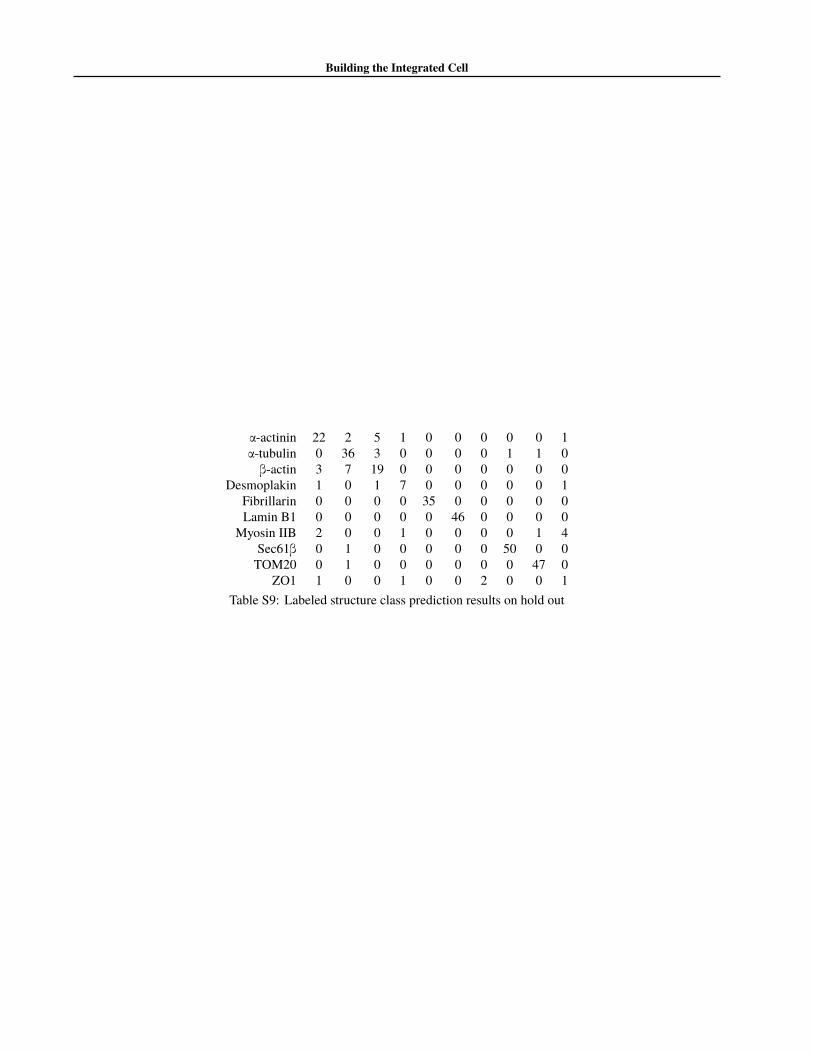
While classification is not our primary use-case, it is aworthwhile benchmark of a well-functioning multi-classgenerative model. To evaluate the performance of the class-label identification of Encr,s we compared the results of thepredicted labels and true labels on our hold out set. Asummary of the results of our multinomial classificationtask is shown in table S9. As seen in the table, our modelis able to accurately classify most structure, and has troubleonly on the poorly sampled or underrepresented classes.

3.4.4. Integrating Cell Images

Conditional upon the cell and nuclear shape, we predict themost likely position of any particular structure via algo-rithm 3. Some examples of the maximum likelihood esti-mate of structure localization given cell and nuclear shapesis shown in figure 3.

4. DiscussionBuildingmodels that capture relationships between themor-phology and organization of cell structures is a difficultproblem. While previous research has focused on con-

Figure 3: Most probable localization patterns predicted forselected cells for each structure (rows, top to bottom, struc-ture as labeled, shown in yellow). The first 5 columns showthe maximum likelihood of localization for each structure,given the cell and nuclear shape. The last column (far right)shows an experimentally observed cell with that labeledstructure for comparison. As before, reference structures,cell membrane and nucleus (DNA), are in magenta andcyan, respectively. Images have been cropped for visual-ization purposes. Note for example how fibrillarin resideswithin the DNA, and lamin B1 surrounds the DNA. Seefigure S6b for structure channel only.

Building the Integrated Cell

structing application-specific parametric approaches, dueto the the extreme variation in localization among differ-ence structures, these approaches may not be convenient toemploy for all structures under all conditions. Here, wehave presented a nonparametric conditional model of struc-ture organization that generalizes well to a wide variety oflocalization patterns, encodes the variation in cell structureand organization, allows for a probabilistic interpretation ofthe image distribution, and generates high quality syntheticimages.

Our model of cell and subcellular structure differs from pre-vious generative models (Zhao & Murphy, 2007; Peng &Murphy, 2011; Johnson et al., 2015): we directly model thelocalization of fluorescent labels, rather than the detectedobjects and their boundaries. While object segmentationcan be essential in certain contexts, and helpful in oth-ers, when these approaches are not necessary, it can beadvantageous to omit these non-trivial intermediate steps.Our model does not constitute a “cytometric” approach (i.e.counting objects), but due to the fact that we are directlymodeling the localization of signal, we drastically reducethe modeling time by minimizing the amount of segmen-tation and the task of evaluating this segmentation withrespect to the “ground truth”.

Even considering these these differences, our model is com-patible with existing frameworks and will allow for mixedparametric and non-parametric localization relationships,where our model can be used for predicting localization ofstructures when an appropriate parametric representationmay not exist.

Our model permits several straightforward extensions, in-cluding the obvious extension to modeling cells in threedimensions. Because of the flexibility of our latent-spacerepresentation, we can potentially encode information suchas position in the cell cycle, or along a differentiation path-way. Given sufficient information, it would be possibleto encode a representation of “structure space” to predictthe localization of unobserved structures, or “perturbationspace”, such as in (Paolini et al., 2006), and potentially cou-ple this with active learning approaches (Naik et al., 2016)to build models that learn and encode the localization ofdiverse subcellular structures under different conditions.

Software and DataThe code for running the models used in this work is avail-able at https://github.com/AllenCellModeling/torch_integrated_cell

The data used to train the model is available at s3://aics.integrated.cell.arxiv.paper.data.

AcknowledgementsWe would like to thank Robert F. Murphy, Julie The-riot, Rick Horwitz, Graham Johnson, Forrest Collman,Sharmishtaa Seshamani and Fuhui Long for their helpfulcomments, suggestions, and support in the preparation ofthe manuscript.

Furthermore, we would like to thank all members of theAllen Institute for Cell Science team, who generated andcharacterized the gene-edited cell lines, developed image-based assays, and recorded the high replicate data sets suit-able for modeling. We particularly thank Liya Ding forsegmentation data. These contributions were absolutelycritical for model development.

We would like to thank Paul G. Allen, founder of the AllenInstitute for Cell Science, for his vision, encouragement andsupport.

Author ContributionsGRJ conceived, designed and implemented all experiments.GRJ, RMD, and MMM wrote the paper.

Building the Integrated Cell

ReferencesArulkumaran, Kai. Autoencoders, 2017. URL https://github.com/Kaixhin/Autoencoders.

Boland,Michael V andMurphy, Robert F. A neural networkclassifier capable of recognizing the patterns of all majorsubcellular structures in fluorescence microscope imagesof hela cells. Bioinformatics, 17(12):1213–1223, 2001.

Carpenter, Anne E, Jones, Thouis R, Lamprecht, Michael R,Clarke, Colin, Kang, In Han, Friman, Ola, Guertin,David A, Chang, Joo Han, Lindquist, Robert A, Moffat,Jason, Golland, Polina, and Sabatini, David M. CellPro-filer: image analysis software for identifying and quan-tifying cell phenotypes. Genome biology, 7(10):R100,2006.

Collobert, Ronan, Kavukcuoglu, Koray, and Farabet, ClÃľ-ment. Torch7: A matlab-like environment for machinelearning, 2011.

Donovan, Rory M, Tapia, Jose-Juan, Sullivan, Devin P,Faeder, James R, Murphy, Robert F, Dittrich, Markus,and Zuckerman, Daniel M. Unbiased rare event sam-pling in spatial stochastic systems biology models usinga weighted ensemble of trajectories. PLoS computationalbiology, 12(2):e1004611, 2016.

Goodfellow, Ian J, Pouget-Abadie, Jean, Mirza, Mehdi,Xu, Bing, Warde-Farley, David, Ozair, Sherjil, Courville,Aaron, and Bengio, Yoshua. Generative Adversarial Net-works. arXiv.org, June 2014.

Johnson, G R, Buck, T E, Sullivan, D P, Rohde, G K, andMurphy, R F. Joint modeling of cell and nuclear shapevariation. Molecular Biology of the Cell, 26(22):4046–4056, November 2015.

Kim, Min-Sik, Pinto, Sneha M, Getnet, Derese, Niru-jogi, Raja Sekhar, Manda, Srikanth S, Chaerkady,Raghothama, Madugundu, Anil K, Kelkar,Dhanashree S, Isserlin, Ruth, Jain, Shobhit, et al.A draft map of the human proteome. Nature, 509(7502):575–581, 2014.

Kingma, Diederik P and Ba, Jimmy. Adam: A Method forStochastic Optimization. arXiv.org, December 2014.

Larsen, Anders Boesen Lindbo, Sønderby, Søren Kaae,Larochelle, Hugo, and Winther, Ole. Autoencoding be-yond pixels using a learned similarity metric. arXiv.org,December 2015.

Makhzani, Alireza, Shlens, Jonathon, Jaitly, Navdeep,Goodfellow, Ian, and Frey, Brendan. Adversarial Au-toencoders. arXiv.org, November 2015.

Murphy, R F. Location proteomics: a systems approach tosubcellular location. Biochemical Society transactions,33(Pt 3):535–538, June 2005.

Naik, Armaghan W, Kangas, Joshua D, Sullivan, Devin P,and Murphy, Robert F. Active machine learning-drivenexperimentation to determine compound effects on pro-tein patterns. eLife, 5:e10047, February 2016.

Paolini, Gaia V, Shapland, Richard H B, van Hoorn,Willem P, Mason, Jonathan S, and Hopkins, Andrew L.Global mapping of pharmacological space. Naturebiotechnology, 24(7):805–815, July 2006.

Peng, Tao and Murphy, Robert F. Image-derived, three-dimensional generative models of cellular organization.Cytometry Part A, 79A(5):383–391, April 2011.

Radford, Alec, Metz, Luke, and Chintala, Soumith. Un-supervised Representation Learning with Deep Convo-lutional Generative Adversarial Networks. arXiv.org,November 2015.

Rajaram, Satwik, Pavie, Benjamin, Wu, Lani F, andAltschuler, Steven J. PhenoRipper: software for rapidlyprofiling microscopy images. Nature Methods, 9(7):635–637, June 2012.

Salimans, Tim, Goodfellow, Ian, Zaremba, Wojciech, Che-ung, Vicki, Radford, Alec, and Chen, Xi. ImprovedTechniques for Training GANs. arXiv.org, June 2016.

Sønderby, Casper Kaae, Caballero, Jose, Theis, Lucas, Shi,Wenzhe, and Huszár, Ferenc. Amortised MAP Inferencefor Image Super-resolution. arXiv.org, October 2016.

Zhao, Ting and Murphy, Robert F. Automated learningof generative models for subcellular location: Buildingblocks for systems biology. Cytometry Part A, 71A(12):978–990, 2007.

Building the Integrated Cell

A. Supplementary Figures

Building the Integrated Cell

Figure S1: Image input (rows 1 and 3) and reconstruction (rows 2 and 4) from the reference model, showing training set(above two rows), and test set (bottom two rows).

Figure S2: Image input (rows 1 and 3) and reconstruction (rows 2 and 4) from the structure model, showing training set(above two rows), and test set (bottom two rows).

(a) (b)

Figure S3: Training curves for the training of the reference model (a) and conditional model (b)

Building the Integrated Cell

(a) (b)

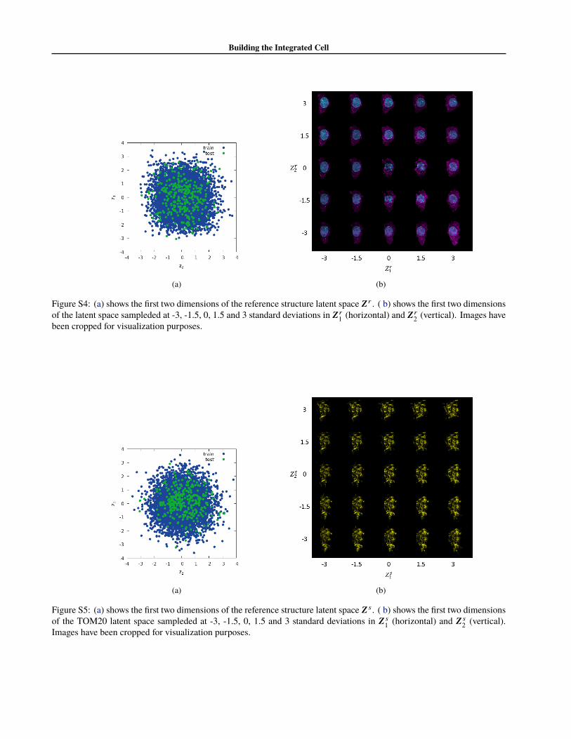
Figure S4: (a) shows the first two dimensions of the reference structure latent space Zr . ( b) shows the first two dimensionsof the latent space sampleded at -3, -1.5, 0, 1.5 and 3 standard deviations in Zr

1 (horizontal) and Zr2 (vertical). Images have

been cropped for visualization purposes.

(a) (b)

Figure S5: (a) shows the first two dimensions of the reference structure latent space Z s . ( b) shows the first two dimensionsof the TOM20 latent space sampleded at -3, -1.5, 0, 1.5 and 3 standard deviations in Z s

1 (horizontal) and Z s2 (vertical).

Images have been cropped for visualization purposes.

Building the Integrated Cell

(a) (b)

Figure S6: (a) Example structure channels for each of the 10 labeled structures in this paper and (b) predicted most probablelocalization patterns for selected cells from each labeled pattern. The first 5 columns show the maximum likelihoodlocalization for the corresponding structures given the the same cell and nuclear shape. The last column shows a observedcell with that labeled structure. Rows correspond to structure types. Images have been cropped for visualization purposes.

Building the Integrated Cell

B. Model Architectures

4 × 4 64 conv ↓ BNorm PReLU4 × 4 128 conv ↓ BNorm PReLU4 × 4 256 conv ↓ BNorm PReLU4 × 4 512 conv ↓ BNorm PReLU4 × 4 1024 conv ↓ BNorm PReLU4 × 4 1024 conv ↓ BNorm PReLU|Zr | FC BNorm

Table S1: Architecture of Encr

1024 FC BNorm PReLU4 × 4 1024 conv ↑ BNorm PReLU4 × 4 512 conv ↑ BNorm PReLU4 × 4 256 conv ↑ BNorm PReLU4 × 4 128 conv ↑ BNorm PReLU4 × 4 64 conv ↑ BNorm PReLU4 × 4 |r | conv ↑ BNorm sigmoid

Table S2: Architecture of Decr

1024 FC Leaky RelU1024 FC BNorm Leaky RelU512 FC BNorm Leaky RelU1 FC Sigmoid

Table S3: Architecture of EncDr and EncDs

+White Noise σ = 0.054 × 4 64 conv ↓ BNorm LeakyReLU4 × 4 128 conv ↓ BNorm LeakyReLU4 × 4 256 conv ↓ BNorm LeakyReLU4 × 4 512 conv ↓ BNorm LeakyReLU4 × 4 512 conv ↓ BNorm LeakyReLU4 × 4 1 conv ↓ sigmoid

Table S4: Architecture of DecDr

4 × 4 64 conv ↓ BNorm PReLU4 × 4 128 conv ↓ BNorm PReLU4 × 4 256 conv ↓ BNorm PReLU4 × 4 512 conv ↓ BNorm PReLU4 × 4 1024 conv ↓ BNorm PReLU4 × 4 1024 conv ↓ BNorm PReLU{K FC, |Zr | FC, |Zs | FC} {BNorm, BNorm, BNorm} {Softmax, , }

Table S5: Architecture of Encr,s

1024 FC BNorm PReLU4 × 4 1024 conv ↑ BNorm PReLU4 × 4 512 conv ↑ BNorm PReLU4 × 4 256 conv ↑ BNorm PReLU4 × 4 128 conv ↑ BNorm PReLU4 × 4 64 conv ↑ BNorm PReLU4 × 4 |r + s | conv ↑ BNorm sigmoid

Table S6: Architecture of Decr,s

+White Noise σ = 0.054 × 4 64 conv ↓ BNorm LeakyReLU4 × 4 128 conv ↓ BNorm LeakyReLU4 × 4 256 conv ↓ BNorm LeakyReLU4 × 4 512 conv ↓ BNorm LeakyReLU4 × 4 512 conv ↓ BNorm LeakyReLU4 × 4 K+1 conv ↓ sigmoid

Table S7: Architecture of DecDr,s

Building the Integrated Cell

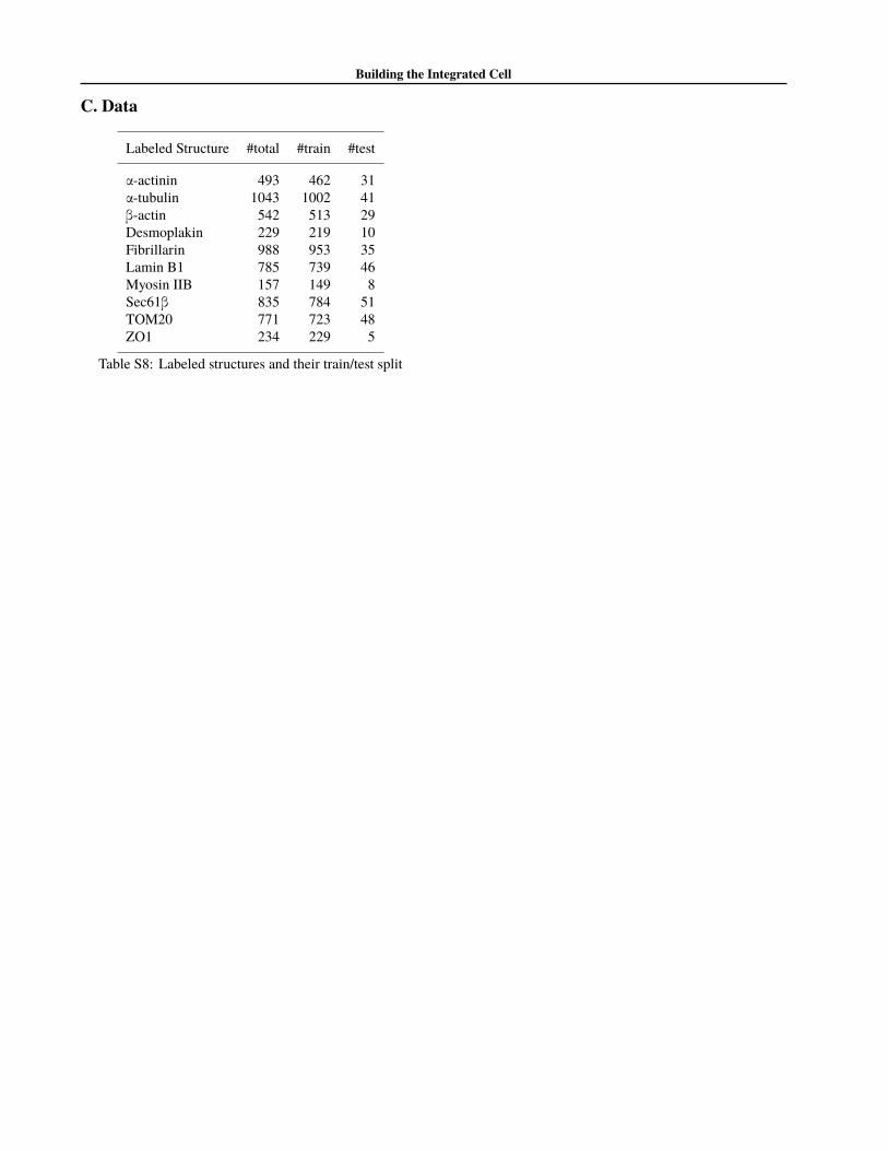
C. Data

Labeled Structure #total #train #test

α-actinin 493 462 31α-tubulin 1043 1002 41β-actin 542 513 29Desmoplakin 229 219 10Fibrillarin 988 953 35Lamin B1 785 739 46Myosin IIB 157 149 8Sec61β 835 784 51TOM20 771 723 48ZO1 234 229 5

Table S8: Labeled structures and their train/test split

Building the Integrated Cell

α-actinin 22 2 5 1 0 0 0 0 0 1α-tubulin 0 36 3 0 0 0 0 1 1 0β-actin 3 7 19 0 0 0 0 0 0 0

Desmoplakin 1 0 1 7 0 0 0 0 0 1Fibrillarin 0 0 0 0 35 0 0 0 0 0Lamin B1 0 0 0 0 0 46 0 0 0 0

Myosin IIB 2 0 0 1 0 0 0 0 1 4Sec61β 0 1 0 0 0 0 0 50 0 0TOM20 0 1 0 0 0 0 0 0 47 0

ZO1 1 0 0 1 0 0 2 0 0 1Table S9: Labeled structure class prediction results on hold out