Conditional Random Fields - DISI, University of Trentopasserini/teaching/2010-2011/SRL/slides/crf/... · Statistical relational learning Conditional Random Fields. Generative vs discriminative

Conditional Random Fields

Andrea [email protected]

Statistical relational learning


Generative vs discriminative models

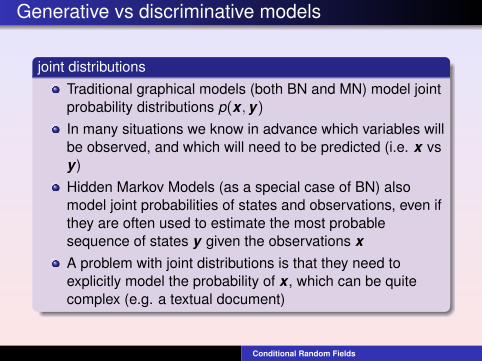
joint distributionsTraditional graphical models (both BN and MN) model jointprobability distributions p(x ,y)

In many situations we know in advance which variables willbe observed, and which will need to be predicted (i.e. x vsy)Hidden Markov Models (as a special case of BN) alsomodel joint probabilities of states and observations, even ifthey are often used to estimate the most probablesequence of states y given the observations xA problem with joint distributions is that they need toexplicitly model the probability of x , which can be quitecomplex (e.g. a textual document)



x1 xi xn

yn−1 n n+1

xn−1 xn xn+1

1 y2

x1 x2

y y yy

Naive Bayes Hidden Markov Model

generative modelsDirected graphical models are called generative when thejoint probability decouples as p(x ,y) = p(x |y)p(y)

The dependencies between input and output are only fromthe latter to the former: the output generates the inputNaive Bayes classifiers and Hidden Markov Models areboth generative models



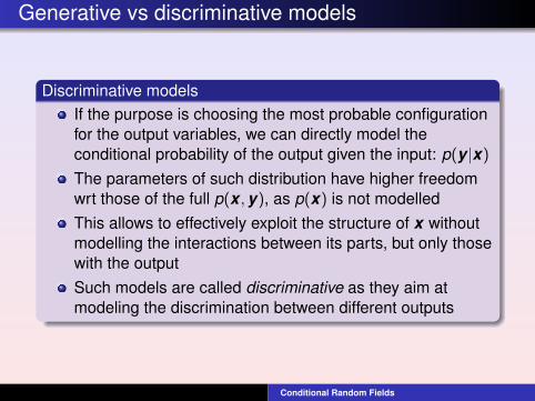
Discriminative modelsIf the purpose is choosing the most probable configurationfor the output variables, we can directly model theconditional probability of the output given the input: p(y |x)

The parameters of such distribution have higher freedomwrt those of the full p(x ,y), as p(x) is not modelledThis allows to effectively exploit the structure of x withoutmodelling the interactions between its parts, but only thosewith the outputSuch models are called discriminative as they aim atmodeling the discrimination between different outputs


Conditional Random Fields (CRF, Lafferty et al. 2001)

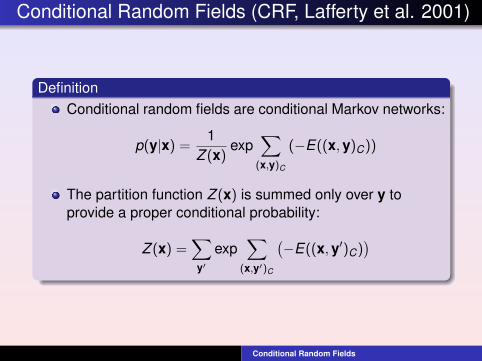
DefinitionConditional random fields are conditional Markov networks:

p(y|x) =1

Z (x)exp

∑(x,y)C

(−E((x,y)C))

The partition function Z (x) is summed only over y toprovide a proper conditional probability:

Z (x) =∑y′

exp∑

(x,y′)C

(−E((x,y′)C)

)



Feature functions

p(y|x) =1

Z (x)exp

∑(x,y)C

K∑k=1

λk fk ((x,y)C)

The negated energy function is often written simply as aweighted sum of real-valued feature functionsEach feature function should capture a certaincharacteristic of the clique variables


Linear chain CRF

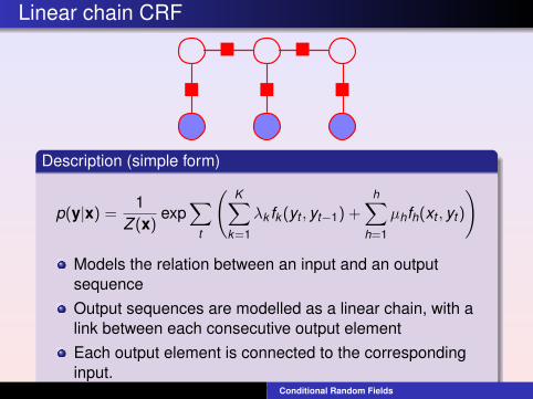
Description (simple form)

p(y|x) =1

Z (x)exp

∑t

(K∑

k=1

λk fk (yt , yt−1) +h∑

h=1

µhfh(xt , yt )

)

Models the relation between an input and an outputsequenceOutput sequences are modelled as a linear chain, with alink between each consecutive output elementEach output element is connected to the correspondinginput.


Linear chain CRF

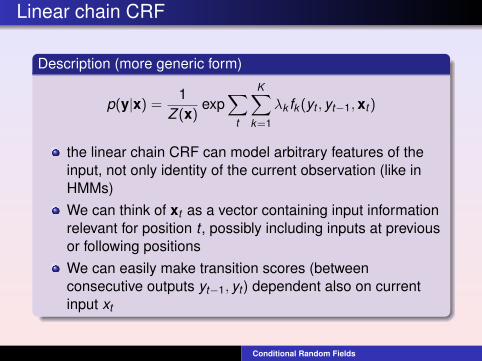
Description (more generic form)

p(y|x) =1

Z (x)exp

∑t

K∑k=1

λk fk (yt , yt−1,xt )

the linear chain CRF can model arbitrary features of theinput, not only identity of the current observation (like inHMMs)We can think of xt as a vector containing input informationrelevant for position t , possibly including inputs at previousor following positionsWe can easily make transition scores (betweenconsecutive outputs yt−1, yt ) dependent also on currentinput xt


Linear chain CRF

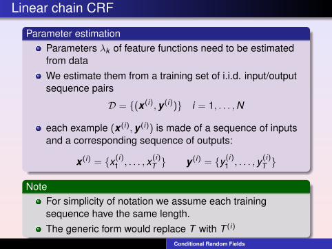
Parameter estimationParameters λk of feature functions need to be estimatedfrom dataWe estimate them from a training set of i.i.d. input/outputsequence pairs

D = {(x (i),y (i))} i = 1, . . . ,N

each example (x (i),y (i)) is made of a sequence of inputsand a corresponding sequence of outputs:

x (i) = {x (i)1 , . . . , x (i)

T } y (i) = {y (i)1 , . . . , y (i)

T }

NoteFor simplicity of notation we assume each trainingsequence have the same length.The generic form would replace T with T (i)


Parameter estimation

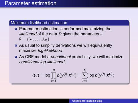
Maximum likelihood estimationParameter estimation is performed maximizing thelikelihood of the data D given the parametersθ = {λ1, . . . , λK}As usual to simplify derivations we will equivalentlymaximize log-likelihoodAs CRF model a conditional probability, we will maximizeconditional log-likelihood:

`(θ) = logN∏

i=1

p(y (i)|x (i)) =N∑

i=1

log p(y (i)|x (i))



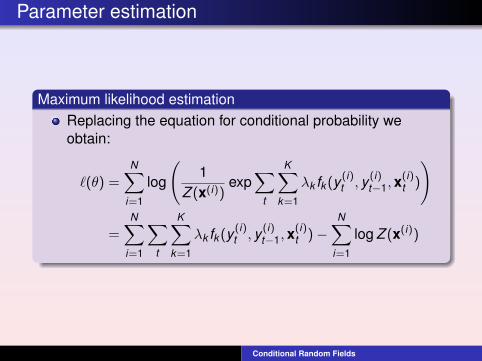
Maximum likelihood estimationReplacing the equation for conditional probability weobtain:

`(θ) =N∑

i=1

log

(1

Z (x(i))exp

∑t

K∑k=1

λk fk (y (i)t , y (i)

t−1,x(i)t )

)

=N∑

i=1

∑t

K∑k=1


t−1,x(i)t )−

N∑i=1

log Z (x(i))


Gradient of the likelihood

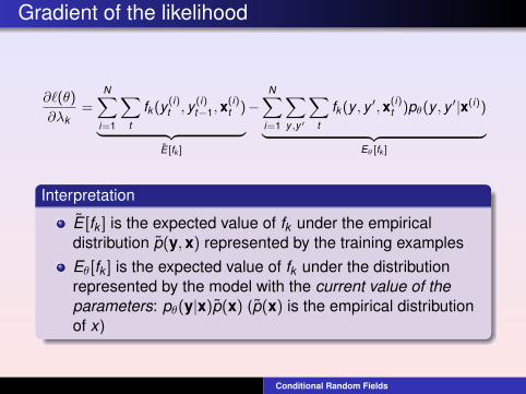
∂`(θ)

∂λk=

N∑i=1

∑t

fk (y (i)t , y (i)

t−1,x(i)t )︸︷︷︸

E [fk ]

−N∑

i=1

∑y,y ′

∑t

fk (y , y ′,x(i)t )pθ(y , y ′|x(i))︸︷︷︸

Eθ [fk ]

Interpretation

E [fk ] is the expected value of fk under the empiricaldistribution p(y,x) represented by the training examplesEθ[fk ] is the expected value of fk under the distributionrepresented by the model with the current value of theparameters: pθ(y|x)p(x) (p(x) is the empirical distributionof x)


Gradient of the likelihood

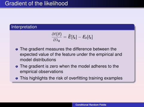
Interpretation

∂`(θ)

∂λk= E [fk ]− Eθ[fk ]

The gradient measures the difference between theexpected value of the feature under the empirical andmodel distributionsThe gradient is zero when the model adheres to theempirical observationsThis highlights the risk of overfitting training examples



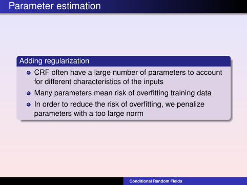
Adding regularization

CRF often have a large number of parameters to accountfor different characteristics of the inputsMany parameters mean risk of overfitting training dataIn order to reduce the risk of overfitting, we penalizeparameters with a too large norm



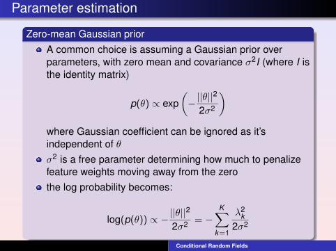
Zero-mean Gaussian priorA common choice is assuming a Gaussian prior overparameters, with zero mean and covariance σ2I (where I isthe identity matrix)

p(θ) ∝ exp(−||θ||

2

2σ2

)where Gaussian coefficient can be ignored as it’sindependent of θσ2 is a free parameter determining how much to penalizefeature weights moving away from the zerothe log probability becomes:

log(p(θ)) ∝ −||θ||2

2σ2 = −K∑

k=1

λ2k

2σ2



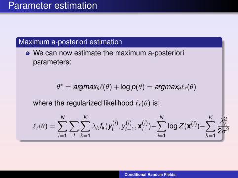
Maximum a-posteriori estimationWe can now estimate the maximum a-posterioriparameters:

θ∗ = argmaxθ`(θ) + log p(θ) = argmaxθ`r (θ)

where the regularized likelihood `r (θ) is:

`r (θ) =N∑

i=1

∑t

K∑k=1


t−1,x(i)t )−

N∑i=1

log Z (x(i))−K∑

k=1

λ2k

2σ2



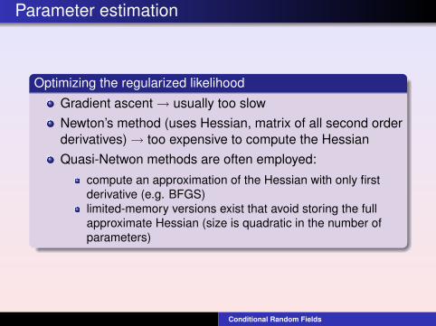
Optimizing the regularized likelihood

Gradient ascent→ usually too slowNewton’s method (uses Hessian, matrix of all second orderderivatives)→ too expensive to compute the HessianQuasi-Netwon methods are often employed:

compute an approximation of the Hessian with only firstderivative (e.g. BFGS)limited-memory versions exist that avoid storing the fullapproximate Hessian (size is quadratic in the number ofparameters)


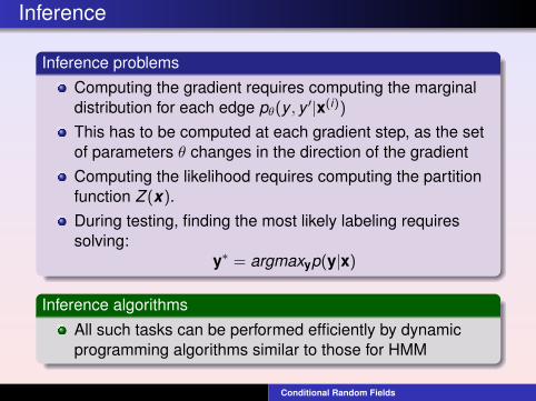
Inference

Inference problemsComputing the gradient requires computing the marginaldistribution for each edge pθ(y , y ′|x(i))

This has to be computed at each gradient step, as the setof parameters θ changes in the direction of the gradientComputing the likelihood requires computing the partitionfunction Z (x).During testing, finding the most likely labeling requiressolving:

y∗ = argmaxyp(y|x)

Inference algorithmsAll such tasks can be performed efficiently by dynamicprogramming algorithms similar to those for HMM


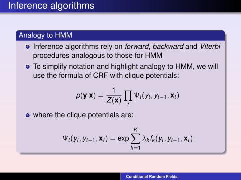
Inference algorithms

Analogy to HMMInference algorithms rely on forward, backward and Viterbiprocedures analogous to those for HMMTo simplify notation and highlight analogy to HMM, we willuse the formula of CRF with clique potentials:

p(y|x) =1

Z (x)

∏t

Ψt (yt , yt−1,xt )

where the clique potentials are:

Ψt (yt , yt−1,xt ) = expK∑

k=1

λk fk (yt , yt−1,xt )



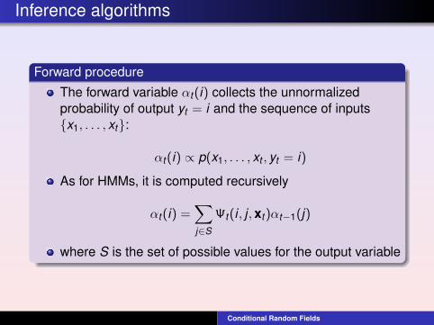
Forward procedure

The forward variable αt (i) collects the unnormalizedprobability of output yt = i and the sequence of inputs{x1, . . . , xt}:

αt (i) ∝ p(x1, . . . , xt , yt = i)

As for HMMs, it is computed recursively

αt (i) =∑j∈S

Ψt (i , j ,xt )αt−1(j)

where S is the set of possible values for the output variable



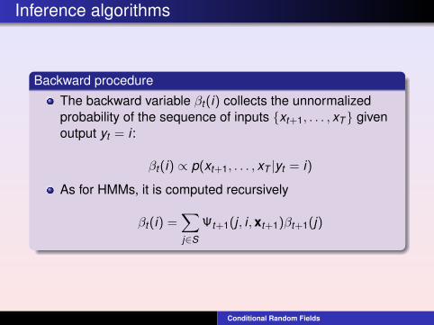
Backward procedure

The backward variable βt (i) collects the unnormalizedprobability of the sequence of inputs {xt+1, . . . , xT} givenoutput yt = i :

βt (i) ∝ p(xt+1, . . . , xT |yt = i)

As for HMMs, it is computed recursively

βt (i) =∑j∈S

Ψt+1(j , i ,xt+1)βt+1(j)


Forward/backward procedures

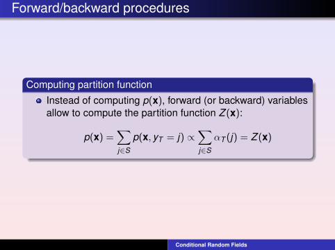
Computing partition function

Instead of computing p(x), forward (or backward) variablesallow to compute the partition function Z (x):

p(x) =∑j∈S

p(x, yT = j) ∝∑j∈S

αT (j) = Z (x)


Forward/backward procedures

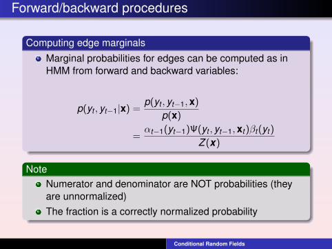
Computing edge marginalsMarginal probabilities for edges can be computed as inHMM from forward and backward variables:

p(yt , yt−1|x) =p(yt , yt−1,x)

p(x)

=αt−1(yt−1)Ψ(yt , yt−1,xt )βt (yt )

Z (x)

NoteNumerator and denominator are NOT probabilities (theyare unnormalized)The fraction is a correctly normalized probability


Viterbi decoding

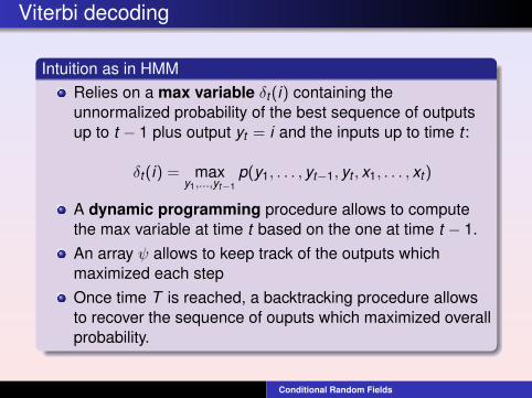
Intuition as in HMMRelies on a max variable δt (i) containing theunnormalized probability of the best sequence of outputsup to t − 1 plus output yt = i and the inputs up to time t :

δt (i) = maxy1,...,yt−1

p(y1, . . . , yt−1, yt , x1, . . . , xt )

A dynamic programming procedure allows to computethe max variable at time t based on the one at time t − 1.An array ψ allows to keep track of the outputs whichmaximized each stepOnce time T is reached, a backtracking procedure allowsto recover the sequence of ouputs which maximized overallprobability.


Viterbi decoding

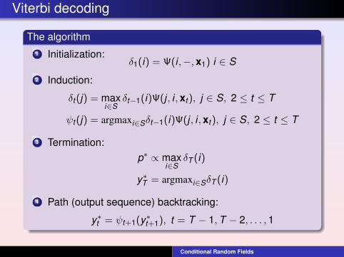
The algorithm1 Initialization:

δ1(i) = Ψ(i ,−,x1) i ∈ S

2 Induction:

δt (j) = maxi∈S

δt−1(i)Ψ(j , i ,xt ), j ∈ S, 2 ≤ t ≤ T

ψt (j) = argmaxi∈Sδt−1(i)Ψ(j , i ,xt ), j ∈ S, 2 ≤ t ≤ T

3 Termination:p∗ ∝ max

i∈SδT (i)

y∗T = argmaxi∈SδT (i)

4 Path (output sequence) backtracking:

y∗t = ψt+1(y∗t+1), t = T − 1,T − 2, . . . ,1


Viterbi decoding

NoteThere is no need for normalization as we are onlyinterested in best output sequence, not its probability


Application example

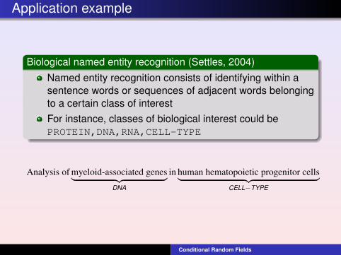
Biological named entity recognition (Settles, 2004)Named entity recognition consists of identifying within asentence words or sequences of adjacent words belongingto a certain class of interestFor instance, classes of biological interest could bePROTEIN,DNA,RNA,CELL-TYPE

Analysis of myeloid-associated genes︸︷︷︸DNA

in human hematopoietic progenitor cells︸︷︷︸CELL−TYPE


Biological named entity recognition

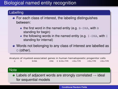
LabellingFor each class of interest, the labeling distinguishesbetween:

the first word in the named entity (e.g. B-DNA, with Bstanding for begin)the following words in the named entity (e.g. I-DNA, with Istanding for internal)

Words not belonging to any class of interest are labelled asO (other).

Analysis of myeloid-associated genes in human hematopoietic progenitor cellsO B-DNA I-DNA B-CELL-TYPE I-CELL-TYPEO O I-CELL-TYPE I-CELL-TYPE

NoteLabels of adjacent words are strongly correlated→ idealfor sequential models



Feature functions: dictionaryThe simplest set of feature functions consists of dictionaryentries.Each feature would model the observation of a certainword and its class assignment, possibly together to theclass assignment of the previous word:

fk (yt , yt−1,xt ) =

1 if xt = cells ∧ yt = CELL-TYPE

∧ yt−1 = CELL-TYPE0 otherwise

Note that the model will have distinct features for theoccurrence of the word cells in different labeling contextsA higher weight λk will be arguably learned for observingthe feature in the CELL-TYPE labelling context wrt otherones.



Feature functions: dictionaryMost dictionary features will be very sparse, with very lowoccurrence in both training data and novel test ones.Very sparse features will be probably receive low or zeroweight, also as an effect of regularization.Fewer relevant dictionary words (e.g. cell, protein,common verbs) should receive higher (positive or negative)weight if found to discriminate between classes in trainingdata.Anyhow some properties common to different words couldalso be found discriminant



Feature functions: orthographic features

Capitalization is often associated to named entities morethan other words (e.g. mRNA)Alphanumeric strings are typically used to identify specificproteins, genes in biological databases (e.g. 7RSA)Dashes often appear in complex compound words (e.g.myeloid-associated)Each such feature can be encoded with a separate function



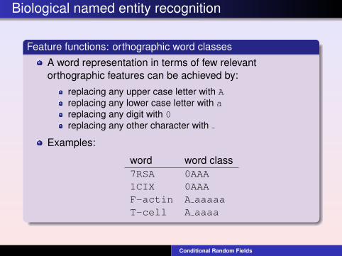
Feature functions: orthographic word classesA word representation in terms of few relevantorthographic features can be achieved by:

replacing any upper case letter with Areplacing any lower case letter with areplacing any digit with 0replacing any other character with

Examples:

word word class7RSA 0AAA1CIX 0AAAF-actin A aaaaaT-cell A aaaa



Feature functions: neighbouring wordsFeatures related to xt are not limited to characteristics ofthe word at position tFor instance, context features can model the identity of theword together to those of the preceding and following onesThe same can be done for other characteristics of words,such as word classes, presence of dashesInformation on neighbouring words can be combined inarbitrary way to create features deemed relevant (e.g. acapitalized word preceded by and article as in theATPase)



Feature functions: semantic featuresWhen available, semantic information can strongly help inbuilding disambiguating featuresFor instance, amino-acids codes are often capitalized orhave capitalized initial (e.g. CYS, His)Such strings could be wrongly identified as named entitiesof one of the classes.An explicit feature representing an amino-acid code couldbe added to help disambiguation.


Conditional random fields

Parameter tying

All cliques (yt , yt−1, xt ) in linear-chain CRF share the sameset of parameters λk independently of tThis parameter tying allows to:

avoid an explosion of parameters, controlling overfittingapply a learned model to sequences of different length


Conditional random fields

Clique templatesParameter tying can be represented by dividing the set ofcliques C in a factor graph G into clique templates:

C = {C1, . . . ,CP}

all cliques in each clique template Cp share the sameparameters θp

linear chain CRF have a single clique template for all(yt , yt−1, xt )


Generic conditional random fields

Description

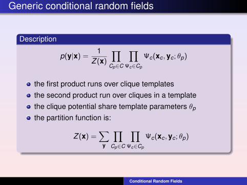
p(y|x) =1

Z (x)

∏Cp∈C

∏Ψc∈Cp

Ψc(xc ,yc ; θp)

the first product runs over clique templatesthe second product run over cliques in a templatethe clique potential share template parameters θp

the partition function is:

Z (x) =∑

y

∏Cp∈C

∏Ψc∈Cp

Ψc(xc ,yc ; θp)



Clique potential

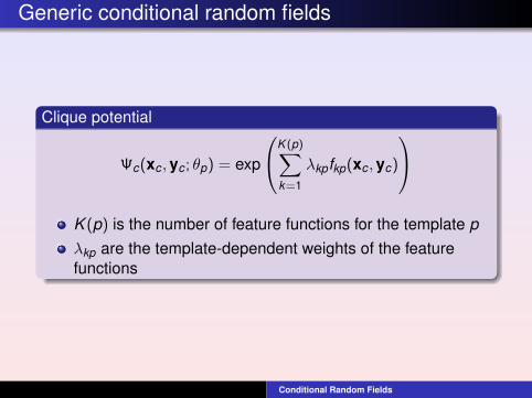
Ψc(xc ,yc ; θp) = exp

K (p)∑k=1

λkpfkp(xc ,yc)

K (p) is the number of feature functions for the template pλkp are the template-dependent weights of the featurefunctions



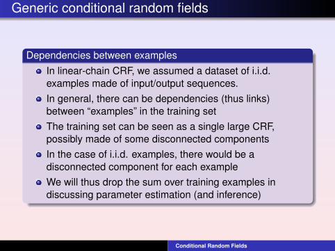
Dependencies between examplesIn linear-chain CRF, we assumed a dataset of i.i.d.examples made of input/output sequences.In general, there can be dependencies (thus links)between “examples” in the training setThe training set can be seen as a single large CRF,possibly made of some disconnected componentsIn the case of i.i.d. examples, there would be adisconnected component for each exampleWe will thus drop the sum over training examples indiscussing parameter estimation (and inference)



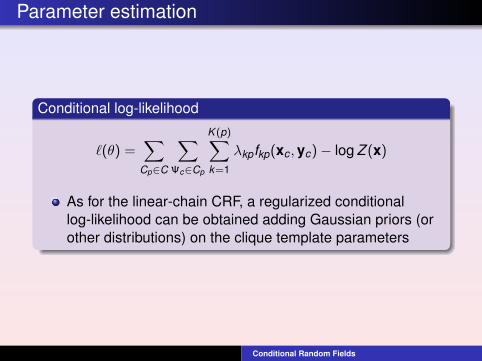
Conditional log-likelihood

`(θ) =∑

Cp∈C

∑Ψc∈Cp

K (p)∑k=1

λkpfkp(xc ,yc)− log Z (x)

As for the linear-chain CRF, a regularized conditionallog-likelihood can be obtained adding Gaussian priors (orother distributions) on the clique template parameters



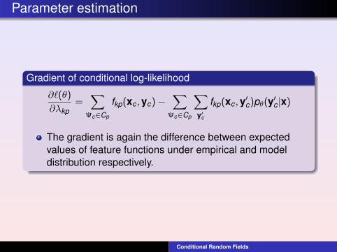
Gradient of conditional log-likelihood

∂`(θ)

∂λkp=∑

Ψc∈Cp

fkp(xc ,yc)−∑

Ψc∈Cp

∑y′c

fkp(xc ,y′c)pθ(y′c |x)

The gradient is again the difference between expectedvalues of feature functions under empirical and modeldistribution respectively.


Inference

Belief propagationBelief propagation is a generalization of forward-backwardprocedure. It computes exact inference on tree-structuredmodelsBelief propagation can also be applied on models withcycles (called loopy belief propagation).Loopy belief propagation is no more exact nor guaranteedto converge, but has successfully been employed as anapproximation strategy.


Inference

Junction treesa tree-structured representation of any graphical modelcan be obtained building a junction treeNodes in junction trees are clusters of variables in theoriginal tree, each link between a pair of clusters has aseparator node with the variables common to both clusters.Exact inference can be achieved on junction trees by beliefpropagationThe algorithm is exponential in the number of variables inthe clusters and is intractable for arbitrary graphs.


Inference

Sampling

Sampling methods compute approximate inferencesampling from the model distributionA number of samples for the variables in the model isgenerated by some random process.The probability of a certain configuration of variable valuesis computed aggregating the samplesThe random process takes time to converge beforegenerating samples from the correct distributionThis can be quite slow if we need to do inference at eachstep of training


Applications

Examplesnamed-entity recognition: detect in a sentence words orsequences of adjacent words referring to a named-entityand classify the entityextract contact information from personal web pages (e.g.name, address, mobile, email)perform multi-label classification modelling dependenciesbetween labelsperform RNA secondary structural alignmentlabel images in computer vision


Skip-chain CRF (Sutton and McCallum, 2004)

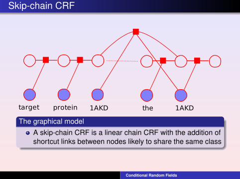
MotivationThe same input can appear multiple times in a certainsequenceSuch multiple instances are often likely to share the samelabelIn named entity recognition, multiple instances of the sameword often refer to the same entity (or class of entities)It would be desirable that the model tends to label suchmultiple occurences consistently


Skip-chain CRF

Modeling long-range dependenciesMultiple instances of the same input can appear atarbitrary distance within the sequenceA linear-chain model needs to pass information along suchdistances in order for difference instances to influence theirrespective labeling decisionsThe problem is in the Markov assumption, that label at timeyt only depends on labels at previous k time instants (withk = 1 in linear chains)Modeling long-range dependencies in such a setting isextremely unlikely


Skip-chain CRF

Adding shortcutsA possible approach to address the problem is by addingshortcut (or skip) links between distant outputs.The number of such links should be limited in order to addlimited complexity to the modelConditional models allow to add links which are dependentof the input contentFor instance, it is possible to add links only betweenoutputs with same inputs (i.e. the shared instances)It is also possible to add links only for instances whichmost likely will share the same class (e.g. capitalizedwords like 7RSA, but not adjectives like human)


Skip-chain CRF

1AKDthetarget protein 1AKD

The graphical model

A skip-chain CRF is a linear chain CRF with the addition ofshortcut links between nodes likely to share the same class


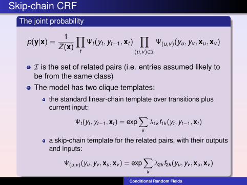
Skip-chain CRFThe joint probability

p(y|x) =1

Z (x)

∏t

Ψt (yt , yt−1,xt )∏

(u,v)∈I

Ψ(u,v)(yu, yv ,xu,xv )

I is the set of related pairs (i.e. entries assumed likely tobe from the same class)The model has two clique templates:

the standard linear-chain template over transitions pluscurrent input:

Ψt (yt , yt−1,xt ) = exp∑

k

λ1k f1k (yt , yt−1,xt )

a skip-chain template for the related pairs, with their outputsand inputs:

Ψ(u,v)(yu, yv ,xu,xv ) = exp∑

k

λ2k f2k (yu, yv ,xu,xv )


Skip-chain CRF

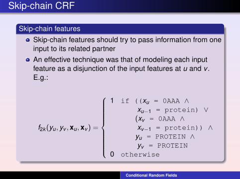
Skip-chain featuresSkip-chain features should try to pass information from oneinput to its related partnerAn effective technique was that of modeling each inputfeature as a disjunction of the input features at u and v .E.g.:

f2k (yu, yv ,xu,xv ) =

1 if ((xu = 0AAA ∧xu−1 = protein) ∨

(xv = 0AAA ∧xv−1 = protein)) ∧yu = PROTEIN ∧yv = PROTEIN

0 otherwise


Skip-chain CRF

InferenceSkip links introduce loops in the graphical model, makingexact inference intractable in generalFurthemore, loops can be long and overlapping, andmaximal cliques in junction trees can be too large to betractableApproximate inference by loopy belief propagation wasapplied to train skip-chain CRF with effective results


Factorial CRF (Sutton et al, 2004)

MotivationSequential labelling tasks do not necessarily limit to scalaroutputs at each time instantA sequence of vectors of outputs can represent the desiredoutcomeThis happens for instance when there is a hierarchy ofoutputs


Factorial CRF

Example: POS tagging and chunkingA relevant and hard task in natural language processing isthat of automatically extracting the syntactic structure of asentenceThe first level of such structure consists of assigning thecorrect part-of-speech (POS) tag to each individual word(e.g. verb, noun, pronoun, adjective)A shallow parsing of sentences consists of identifyingchunks of consecutive groups of words representinggrammatical units such as noun or verb phrases.


Factorial CRF

ExampleSentence:He reckons the current account deficit willnarrow to only L1.8 billion in September.

POS tagging:(PRP)He (VBZ)reckons (DT)the (JJ)current(NN)account (NN)deficit (MD)will (VB)narrow(TO)to (RB)only (L)L (CD)1.8 (CD)billion(IN)in (NNP)September (.).

Shallow parsing:[NP He ] [VP reckons ] [NP the currentaccount deficit ] [VP will narrow ] [PP to] [NP only L 1.8 billion ] [PP in ] [NPSeptember ].


Factorial CRF

Example: POS tagging and chunking

POS tagging is often used as a first step for shallowparsing.The two tasks can be accomplished in cascade:

First each word is labelled with its predicted POS tagThen the sequence of words and POS tags is passed to theshallow parser which identifies the chunks

However, an error at the first level (POS tagging) will badlyaffect the performance of the following level (chunking)Such error propagation effect can be dramatic for multiplelevels of labeling.


Factorial CRF

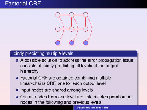
Jointly predicting multiple levelsA possible solution to address the error propagation issueconsists of jointly predicting all levels of the outputhierarchyFactorial CRF are obtained combining multiplelinear-chains CRF, one for each output levelInput nodes are shared among levelsOutput nodes from one level are link to cotemporal outputnodes in the following and previous levels


Factorial CRF

Joint probability

p(y|x) =1

Z (x)

T∏t=1

L∏l=1

Ψt (yt ,l , yt−1,l ,xt )Φt (yt ,l , yt ,l+1,xt )

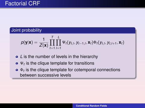
L is the number of levels in the hierarchyΨt is the clique template for transitionsΦt is the clique template for cotemporal connectionsbetween successive levels


Factorial CRF

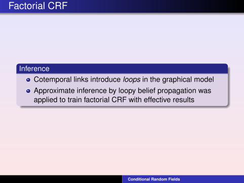
InferenceCotemporal links introduce loops in the graphical modelApproximate inference by loopy belief propagation wasapplied to train factorial CRF with effective results


Tree CRF (Cohn and Blunsom, 2005)

Semantic role labelling

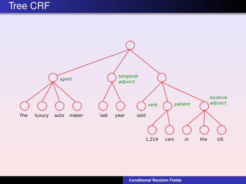
Given a full parse tree, decide which constituents fillsemantic roles (agent, patient, etc) for a given verbTask is to annotate parse structure with role informationA tree CRF is constructed according to the structure of theparse treeEfficient exact inference can be accomplished by beliefpropagation


Tree CRF

The luxury auto maker last year sold

1,214 cars in the US

agenttemporaladjunct

verb patient

locativeadjunct


Resources

ReferencesJohn Lafferty, Andrew McCallum, and Fernando Pereira,Conditional random fields: Probabilistic models forsegmenting and labeling sequence data, ICML 2001.C. Sutton, A. McCallum, An Introduction to ConditionalRandom Fields for Relational Learning, in Introduction toStatistical Relational Learning, L. Getoor and B. Taskar,eds., the MIT Press, 2007.C. Sutton, K. Rohanimanesh, A. McCallum, DynamicConditional Random Fields: Factorized ProbabilisticModels for Labeling and Segmenting Sequence Data,ICML 2004.Trevor Cohn and Philip Blunsom, Semantic Role Labellingwith Tree Conditional Random Fields, CoNLL 2005


Resources

ReferencesJohn Lafferty, Andrew McCallum, and Fernando Pereira,Conditional random fields: Probabilistic models forsegmenting and labeling sequence data, ICML 2001.C. Sutton, A. McCallum, An Introduction to ConditionalRandom Fields for Relational Learning, in Introduction toStatistical Relational Learning, L. Getoor and B. Taskar,eds., the MIT Press, 2007.


Resources

SoftwareCRF++: Yet Another CRF toolkit (sequence labelling)

http://crfpp.sourceforge.net/

Conditional Random Field (CRF) Toolbox for Matlab (1Dchains and 2D lattices)

http://www.cs.ubc.ca/∼murphyk/Software/CRF/crf.html

MALLET: Java package for machine learning applicationsto text. Includes CRF for sequence labelling

http://mallet.cs.umass.edu/

LinksHanna Wallach page on CRF (includes CRF relatedpublications and software)

http://www.inference.phy.cam.ac.uk/hmw26/crf/


Documents

Conditional Random Fields - DISI, University of Trentopasserini/teaching/2010-2011/SRL/slides/crf/... · Statistical relational learning Conditional Random Fields. Generative vs discriminative