Generation of initial molecular dynamics conﬁgurations in ... · September 19, 2007 12:5 Molecular Simulation molConﬁg˙paper Molecular Simulation, Vol. 00, No. 00, DD Month 200x,

September 19, 2007 12:5 Molecular Simulation molConfig˙paper

Molecular Simulation, Vol. 00, No. 00, DD Month 200x, 1–19

Generation of initial molecular dynamics configurations in arbitrary geometries and

in parallel

Graham B. Macpherson∗, Matthew K. Borg and Jason M. Reese

Department of Mechanical Engineering, University of Strathclyde,

Glasgow G1 1XJ, UK(draft September 19, 2007)

A computational pre-processing tool for generating initial configurations of molecules for molecular dynamics simulations in geometriesdescribed by a mesh of unstructured arbitrary polyhedra is described. The mesh is divided into separate zones and each can be filled witha single crystal lattice of atoms. Each zone is filled by creating an expanding cube of crystal unit cells, initiated from an anchor pointfor the lattice. Each unit cell places the appropriate atoms for the user-specified crystal structure and orientation. The cube expandsuntil the entire zone is filled with the lattice; zones with concave and disconnected volumes may be filled. When the mesh is spatiallydecomposed into portions for distributed parallel processing, each portion may be filled independently, meaning that the entire molecularsystem never needs to fit onto a single processor, allowing very large systems to be created. The computational time required to fill azone with molecules scales linearly with the number of cells in the zone for a fixed number of molecules, and better than linearly withthe number of molecules for a fixed number of mesh cells. Our tool, molConfig, has been implemented in the open source C++ codeOpenFOAM.

Keywords: molecular dynamics, nano fluidics, molecular geometry definition, parallel computing, OpenFOAMPACS: 31.15.Qg, 47.11.Mn

1 Introduction and motivation

Molecular Dynamics (MD) simulations in arbitrary geometries defined by a mesh comprising unstructured,arbitrary polyhedral cells, require initial configurations of molecules to be generated corresponding to thevolumes defined by the mesh. This paper describes the algorithms underpinning a pre-processing toolable to create such configurations: molConfig. It is able to fill volumes defined by a zone of the mesh (aset of cells) with a single species crystal lattice of molecules. The user may specify the lattice structure,orientation, density, temperature and average velocity.

To preserve generality in the algorithm description, ‘molecule’ will be used in this paper to mean ‘atom’,‘ion’ or ‘molecule’, i.e. a region being filled with argon atoms, with sodium and chloride ions, or withwhole water molecules would all be referred to as being filled with molecules. The physical context shouldindicate the meaning.

molConfig is written using OpenFOAM [1], an open source C++ toolbox. It provides molecule configu-ration generation for an MD code, also written using OpenFOAM, that performs simulations in meshes ofunstructured arbitrary polyhedra [2]. This type of mesh allows complex, realistic engineering geometriesderived from CAD models to be directly simulated by MD; it is intended for the simulation and designof nano-scale devices. molConfig operates independently on individual portions of a mesh that has beenspatially decomposed to run in parallel, allowing systems comprising very large numbers of molecules tobe created because they never need to all be contained on a single processor. The molecular configurationsare the same whether generated in parallel or in serial; crystal lattices generated in parallel are continuousand defectless across interprocessor boundaries. All parallel decomposition, interprocessor communication(using MPI), and reconstruction is dealt with by OpenFOAM.

∗Corresponding author: [email protected]

Molecular SimulationISSN print/ISSN online c© 200x Taylor & Francis

http://www.tandf.co.uk/journalsDOI:


2 Initial MD configurations

Figure 1. A complex geometry test case: a three-inlet fluid mixing channel. Four zones are defined, the exterior region (left) contains atethered crystal lattice to define the channel walls. The three interior zones (right, one central and two ‘arm’ zones) contain the

molecules representing the liquid. The overall height of the system is 82nm.

1.1 Mesh description

The mesh in OpenFOAM is flexible and powerful: it is unstructured and built from arbitrary polyhedra.From the OpenFOAM user guide [1]:

‘By default OpenFOAM defines a mesh of arbitrary polyhedral cells in 3D, bounded by arbitrary polygonalfaces, i.e. the cells can have an unlimited number of faces where, for each face, there is no limit on the numberof edges nor any restriction on its alignment.’

A list of mesh vertex positions is stored and a list of mesh faces is constructed; each face is an ordered listof vertex numbers. Cells are constructed as a list of face numbers. Cells can be grouped together into zones,each zone representing a region of the domain with common characteristics. Zones are used in molConfig

to define regions to be filled with different crystals.

1.2 Motivation: example application

The motivation for developing a molecular configuration generator for arbitrary geometries is the desire touse MD to simulate systems such as that shown in figure 1. This example case is a three-inlet mixing chan-nel; the geometry was defined using Pro/ENGINEER R© CAD software, the mesh (a mixture of tetrahedral,hexahedral and pyramidal cells) was generated using GAMBIT R©(a commercial mesh generator) then themesh was imported into OpenFOAM. Four zones of cells were defined and the mesh was decomposed into52 portions for parallel processing (see figure 2) each of which was filled with molecules independently.

2 Volume filling algorithm

The algorithm used by molConfig fills any volume, defined by a zone of cells, with a single lattice ofmolecules with specified orientation and alignment. It generates an expanding cube of lattice unit cells,starting from a user-specified position (known as an ‘anchor’ for the lattice), and angled according to auser-specified orientation (see figure 3). Each of these unit cells is populated with molecules corresponding


G. B. Macpherson, M. K. Borg and J. M. Reese 3

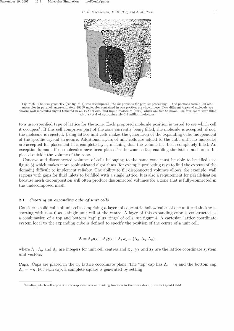
Figure 2. The test geometry (see figure 1) was decomposed into 52 portions for parallel processing — the portions were filled withmolecules in parallel. Approximately 48000 molecules contained in one portion are shown here. Two different types of molecule are

shown: wall molecules (light) tethered in an FCC crystal and liquid molecules (dark) which are free to move. The four zones were filledwith a total of approximately 2.2 million molecules.

to a user-specified type of lattice for the zone. Each proposed molecule position is tested to see which cellit occupies1. If this cell comprises part of the zone currently being filled, the molecule is accepted; if not,the molecule is rejected. Using lattice unit cells makes the generation of the expanding cube independentof the specific crystal structure. Additional layers of unit cells are added to the cube until no moleculesare accepted for placement in a complete layer, meaning that the volume has been completely filled. Anexception is made if no molecules have been placed in the zone so far, enabling the lattice anchors to beplaced outside the volume of the zone.

Concave and disconnected volumes of cells belonging to the same zone must be able to be filled (seefigure 3) which makes more sophisticated algorithms (for example projecting rays to find the extents of thedomain) difficult to implement reliably. The ability to fill disconnected volumes allows, for example, wallregions with gaps for fluid inlets to be filled with a single lattice. It is also a requirement for parallelisationbecause mesh decomposition will often produce disconnected volumes for a zone that is fully-connected inthe undecomposed mesh.

2.1 Creating an expanding cube of unit cells

Consider a solid cube of unit cells comprising n layers of concentric hollow cubes of one unit cell thickness,starting with n = 0 as a single unit cell at the centre. A layer of this expanding cube is constructed asa combination of a top and bottom ‘cap’ plus ‘rings’ of cells, see figure 4. A cartesian lattice coordinatesystem local to the expanding cube is defined to specify the position of the centre of a unit cell,

Λ = Λxxλ + Λyyλ + Λzzλ ≡ (Λx,Λy,Λz) ,

where Λx,Λy and Λz are integers for unit cell centres and xλ, yλ and zλ are the lattice coordinate systemunit vectors.

Caps. Caps are placed in the xy lattice coordinate plane. The ‘top’ cap has Λz = n and the bottom capΛz = −n. For each cap, a complete square is generated by setting

1Finding which cell a position corresponds to is an existing function in the mesh description in OpenFOAM.



2

1

A

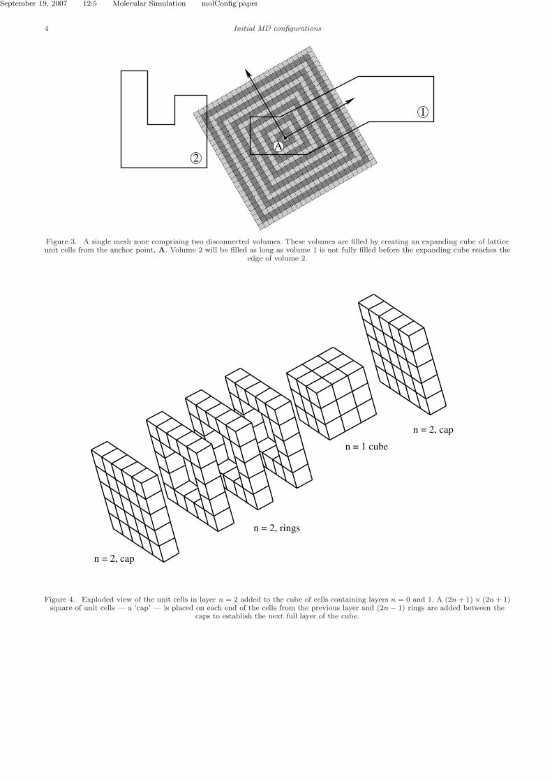
Figure 3. A single mesh zone comprising two disconnected volumes. These volumes are filled by creating an expanding cube of latticeunit cells from the anchor point, A. Volume 2 will be filled as long as volume 1 is not fully filled before the expanding cube reaches the

edge of volume 2.

n = 2, cap

n = 1 cube

n = 2, rings

n = 2, cap

Figure 4. Exploded view of the unit cells in layer n = 2 added to the cube of cells containing layers n = 0 and 1. A (2n + 1) × (2n + 1)square of unit cells — a ‘cap’ — is placed on each end of the cells from the previous layer and (2n − 1) rings are added between the

caps to establish the next full layer of the cube.



Λy = {−n,−n+ 1, . . . , n} ,

and for each value of Λy generate a line of cubes by setting

Λx = {−n,−n+ 1, . . . , n} .

The centre unit cell (n = 0) is a special case and is placed at the lattice coordinate origin.

Rings. There are 2n− 1 rings, with

Λz = {−n+ 1,−n + 2, . . . , n− 1} .

The rings are created by a 2D expanding layer of squares algorithm. The (Λx,Λy) coordinates of the unitcells to be added to the layer of the ring are generated by adding a layer to a square of unit cells. Unitcells are generated along one side of the square and replicated around the other three sides to create thewhole layer. Note that this replication cannot be performed by simply rotating or reflecting the positionsof molecules on one side to create the other three, because the unit cells are generally not rotationallysymmetric.

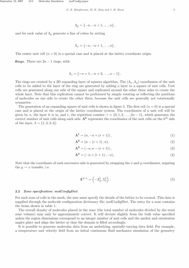
The generation of an expanding square of unit cells is shown in figure 5. The first cell (n = 0) is a specialcase and is placed at the origin of the lattice coordinate system. The coordinates of a unit cell will begiven by n, the layer it is in, and r, the repetition counter: r = {0, 1, 2, . . . , 2n − 1}, which generates thecorrect number of unit cells along each side. Λk represents the coordinates of the unit cells on the kth sideof the layer, k = {1, 2, 3, 4}:

Λ1 = (n,−n+ (r + 1)) , (1)

Λ2 = (n− (r + 1) , n) , (2)

Λ3 = (−n, n− (r + 1)) , (3)

Λ4 = (−n+ (r + 1) ,−n) . (4)

Note that the coordinate of each successive side is generated by swapping the x and y coordinates, negatingthe y → x transfer, i.e.

Λk+1 =(

−Λky ,Λ

kx

)

. (5)

2.2 Zone specification: molConfigDict

For each zone of cells in the mesh, the user must specify the details of the lattice to be created. This data issupplied through the molecule configuration dictionary file: molConfigDict. The entry for a zone containsthe items shown in table 1.

The overall density of molecules placed in the zone (the total number of molecules divided by the totalzone volume) may only be approximately correct. It will deviate slightly from the bulk value specifiedunless the region dimensions correspond to an integer number of unit cells and the anchor and orientationangles place and align the lattice so that the domain is filled accordingly.

It is possible to generate molecular data from an underlying, spatially-varying data field. For example,a temperature and velocity field from an initial continuum fluid mechanics simulation of the geometry



a)

1

2

3

4

5

1 2 3 4 5

b)

1

2

3

4

5

1 2 3 4 5

c)

1

2

3

4

5

1 2 3 4 5

d)

1

2

3

4

5

1 2 3 4 5

Figure 5. The construction of the sides of the square for layers n = {1, 2, 3, 4}. Λ1: vertical, positive x, light-grey. Λ2: horizontal,positive y, dark-grey. Λ3: vertical, negative x, white. Λ4: horizontal, negative y, mid-gray. a) Λ1 for n = 1; b) all sides for n = 1 and

Λ1 for n = 2; c) all sides for n = 2 and Λ

1 for n = 3; d) all sides for n = 3 and Λ1 for n = 4.

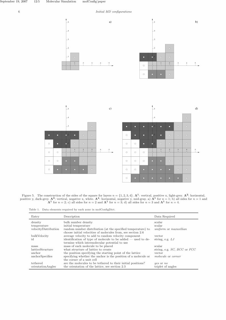
Table 1. Data elements required by each zone in molConfigDict.

Entry Description Data Required

density bulk number density scalartemperature initial temperature scalarvelocityDistribution random number distribution (at the specified temperature) to

choose initial velocities of molecules from, see section 2.6uniform or maxwellian

bulkVelocity average velocity to add to random velocity component vectorid identification of type of molecule to be added — used to de-

termine which intermolecular potential to usestring, e.g. LJ

mass mass of each molecule to be placed scalarlatticeStructure what structure of lattice to create string, e.g. SC, BCC or FCCanchor the position specifying the starting point of the lattice vectoranchorSpecifies specifying whether the anchor is the position of a molecule or

the corner of a unit cellmolecule or corner

tethered are the molecules to be tethered to their initial positions? yes or noorientationAngles the orientation of the lattice, see section 2.3 triplet of angles



using OpenFOAM may be available, and the molecular velocities can be generated using the local valuesof temperature and bulk velocity.

To create a solid wall in a simulation it is often useful to tether molecules into a lattice, for example usinga spring potential [3, 4], so that they retain their structure. If tethered is yes, then the initial locations ofmolecules in this zone will be their tether positions.

In future developments of the utility, realistic crystals will be available in a library. The id, mass anddensity entries will not be necessary, and additional information may be required. For example, for lat-ticeStructure = NaCl, molecules would be placed with the correct structure and spacing for the specifiedtemperature (and possibly pressure), and given ids of Na and Cl, with the appropriate mass and chargeassigned to each.

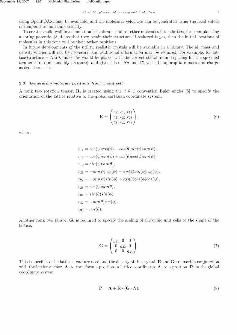
2.3 Generating molecule positions from a unit cell

A rank two rotation tensor, R, is created using the φ, θ, ψ convention Euler angles [5] to specify theorientation of the lattice relative to the global cartesian coordinate system:

R =

r11 r12 r13r21 r22 r23r31 r32 r33

, (6)

where,

r11 = cos(ψ)cos(φ) − cos(θ)sin(φ)sin(ψ),

r12 = cos(ψ)sin(φ) + cos(θ)cos(φ)sin(ψ),

r13 = sin(ψ)sin(θ),

r21 = −sin(ψ)cos(φ) − cos(θ)sin(φ)cos(ψ),

r22 = −sin(ψ)sin(φ) + cos(θ)cos(φ)cos(ψ),

r23 = cos(ψ)sin(θ),

r31 = sin(θ)sin(φ),

r32 = −sin(θ)cos(φ),

r33 = cos(θ).

Another rank two tensor, G, is required to specify the scaling of the cubic unit cells to the shape of thelattice,

G =

g11 0 00 g22 00 0 g33

. (7)

This is specific to the lattice structure used and the density of the crystal. R and G are used in conjunctionwith the lattice anchor, A, to transform a position in lattice coordinates, Λ, to a position, P, in the globalcoordinate system

P = A + R · (G · Λ). (8)



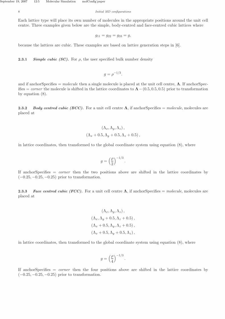
Each lattice type will place its own number of molecules in the appropriate positions around the unit cellcentre. Three examples given below are the simple, body-centred and face-centred cubic lattices where

g11 = g22 = g33 = g,

because the lattices are cubic. These examples are based on lattice generation steps in [6].

2.3.1 Simple cubic (SC). For ρ, the user specified bulk number density

g = ρ−1/3.

and if anchorSpecifies = molecule then a single molecule is placed at the unit cell centre, Λ. If anchorSpec-ifies = corner the molecule is shifted in the lattice coordinates to Λ− (0.5, 0.5, 0.5) prior to transformationby equation (8).

2.3.2 Body centred cubic (BCC). For a unit cell centre Λ, if anchorSpecifies = molecule, molecules areplaced at

(Λx,Λy,Λz) ,

(Λx + 0.5,Λy + 0.5,Λz + 0.5) ,

in lattice coordinates, then transformed to the global coordinate system using equation (8), where

g =(ρ

2

)−1/3.

If anchorSpecifies = corner then the two positions above are shifted in the lattice coordinates by(−0.25,−0.25,−0.25) prior to transformation.

2.3.3 Face centred cubic (FCC). For a unit cell centre Λ, if anchorSpecifies = molecule, molecules areplaced at

(Λx,Λy,Λz) ,

(Λx,Λy + 0.5,Λz + 0.5) ,

(Λx + 0.5,Λy ,Λz + 0.5) ,

(Λx + 0.5,Λy + 0.5,Λz) ,

in lattice coordinates, then transformed to the global coordinate system using equation (8), where

g =(ρ

4

)−1/3.

If anchorSpecifies = corner then the four positions above are shifted in the lattice coordinates by(−0.25,−0.25,−0.25) prior to transformation.



A

minX X

max

Ymax

Ymin

x λ

y λ

OA

Global coordinate system

x

y

C

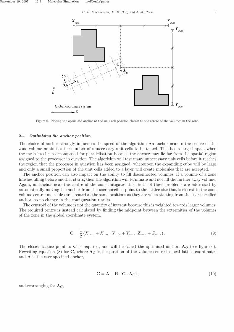
Figure 6. Placing the optimised anchor at the unit cell position closest to the centre of the volumes in the zone.

2.4 Optimising the anchor position

The choice of anchor strongly influences the speed of the algorithm An anchor near to the centre of thezone volume minimises the number of unnecessary unit cells to be tested. This has a large impact whenthe mesh has been decomposed for parallelisation because the anchor may lie far from the spatial regionassigned to the processor in question. The algorithm will test many unnecessary unit cells before it reachesthe region that the processor in question has been assigned, whereupon the expanding cube will be largeand only a small proportion of the unit cells added to a layer will create molecules that are accepted.

The anchor position can also impact on the ability to fill disconnected volumes. If a volume of a zonefinishes filling before another starts, then the algorithm will terminate and not fill the further away volume.Again, an anchor near the centre of the zone mitigates this. Both of these problems are addressed byautomatically moving the anchor from the user-specified point to the lattice site that is closest to the zonevolume centre; molecules are created at the same positions as they are when starting from the user-specifiedanchor, so no change in the configuration results.

The centroid of the volume is not the quantity of interest because this is weighted towards larger volumes.The required centre is instead calculated by finding the midpoint between the extremities of the volumesof the zone in the global coordinate system,

C =1

2(Xmin +Xmax, Ymin + Ymax, Zmin + Zmax) . (9)

The closest lattice point to C is required, and will be called the optimised anchor, AO (see figure 6).Rewriting equation (8) for C, where ΛC is the position of the volume centre in local lattice coordinatesand A is the user specified anchor,

C = A + R· (G ·ΛC) , (10)

and rearranging for ΛC ,



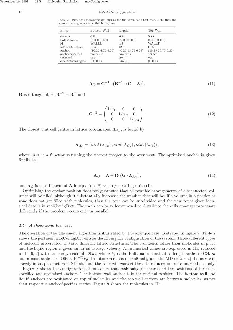
Table 2. Pertinent molConfigDict entries for the three zone test case. Note that the

orientation angles are specified in degrees.

Entry Bottom Wall Liquid Top Wall

density 0.8 0.8 0.85bulkVelocity (0.0 0.0 0.0) (2.0 0.0 0.0) (0.0 0.0 0.0)id WALLB LJ WALLTlatticeStructure FCC SC BCCanchor (16.25 4.75 6.25) (6.25 13.25 6.25) (18.25 20.75 6.25)anchorSpecifies molecule molecule cornertethered yes no yesorientationAngles (30 0 0) (45 0 0) (0 0 0)

ΛC = G−1 ·(

R−1 · (C− A))

. (11)

R is orthogonal, so R−1 = RT and

G−1 =

1/g11 0 00 1/g22 00 0 1/g33

. (12)

The closest unit cell centre in lattice coordinates, ΛAO, is found by

ΛAO= (nint (ΛCx) , nint (ΛCy) , nint (ΛCz)) , (13)

where nint is a function returning the nearest integer to the argument. The optimised anchor is givenfinally by

AO = A + R· (G ·ΛAO) , (14)

and AO is used instead of A in equation (8) when generating unit cells.Optimising the anchor position does not guarantee that all possible arrangements of disconnected vol-

umes will be filled, although it substantially increases the number that will be. If a volume in a particularzone does not get filled with molecules, then the zone can be subdivided and the new zones given iden-tical details in molConfigDict. The mesh can be redecomposed to distribute the cells amongst processorsdifferently if the problem occurs only in parallel.

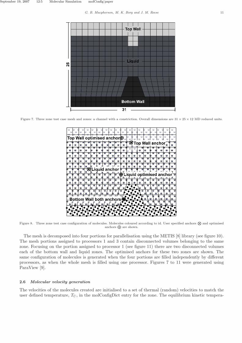
2.5 A three zone test case

The operation of the placement algorithm is illustrated by the example case illustrated in figure 7. Table 2shows the pertinent molConfigDict entries describing the configuration of the system. Three different typesof molecule are created, in three different lattice structures. The wall zones tether their molecules in placeand the liquid region is given an initial average velocity. All numerical values are expressed in MD reducedunits [6, 7] with an energy scale of 120kb, where kb is the Boltzmann constant, a length scale of 0.34nmand a mass scale of 6.6904 × 10−26kg. In future versions of molConfig and the MD solver [2] the user willspecify input parameters in SI units and the code will convert these to reduced units for internal use only.

Figure 8 shows the configuration of molecules that molConfig generates and the positions of the user-specified and optimised anchors. The bottom wall anchor is in the optimal position. The bottom wall andliquid anchors are positioned on top of molecules and the top wall anchors are between molecules, as pertheir respective anchorSpecifies entries. Figure 9 shows the molecules in 3D.



Figure 7. Three zone test case mesh and zones: a channel with a constriction. Overall dimensions are 31 × 25 × 12 MD reduced units.

Figure 8. Three zone test case configuration of molecules. Molecules coloured according to id. User specified anchorsN

and optimisedanchors

L

are shown.

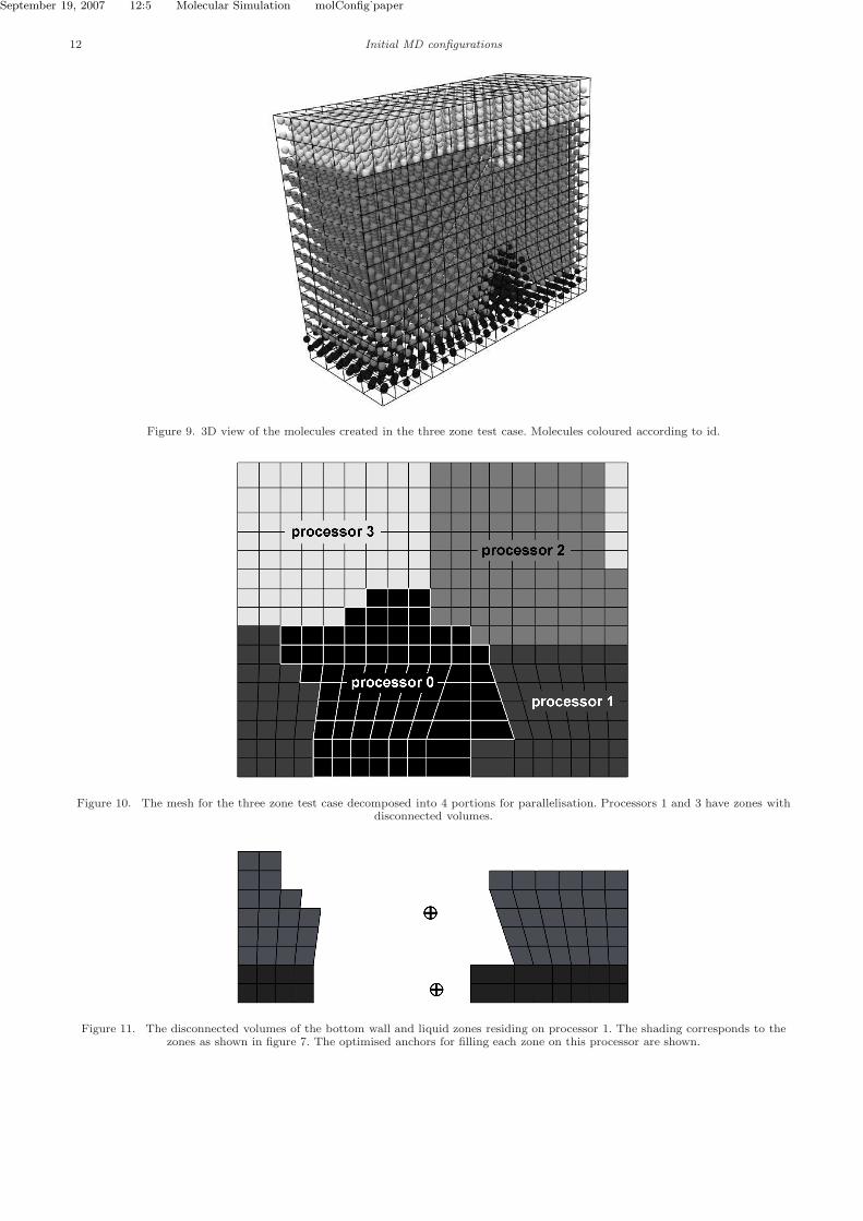
The mesh is decomposed into four portions for parallelisation using the METIS [8] library (see figure 10).The mesh portions assigned to processors 1 and 3 contain disconnected volumes belonging to the samezone. Focusing on the portion assigned to processor 1 (see figure 11) there are two disconnected volumeseach of the bottom wall and liquid zones. The optimised anchors for these two zones are shown. Thesame configuration of molecules is generated when the four portions are filled independently by differentprocessors, as when the whole mesh is filled using one processor. Figures 7 to 11 were generated usingParaView [9].

2.6 Molecular velocity generation

The velocities of the molecules created are initialised to a set of thermal (random) velocities to match theuser defined temperature, TU , in the molConfigDict entry for the zone. The equilibrium kinetic tempera-



Figure 9. 3D view of the molecules created in the three zone test case. Molecules coloured according to id.

Figure 10. The mesh for the three zone test case decomposed into 4 portions for parallelisation. Processors 1 and 3 have zones withdisconnected volumes.

Figure 11. The disconnected volumes of the bottom wall and liquid zones residing on processor 1. The shading corresponds to thezones as shown in figure 7. The optimised anchors for filling each zone on this processor are shown.



ture, T , of a stationary system of NM molecules [7] is then given by

T =1

3NM

NM∑

i=1

miv2i , (15)

in MD reduced units, where mi is the mass of a molecule and vi is the magnitude of its velocity. Thedirection of the velocity assigned to each molecule is random, and the magnitude of each is chosen to givethe correct temperature. The distribution of molecular speeds can either be uniform or Maxwellian.

2.6.1 Uniform distribution. A vector, vr, is created for each molecule which has each of its componentsgenerated by a uniform random number generator returning a value between -1 and 1. The velocity assignedto the molecule, vi, is given by

vi =

√

3TU

mi

vr

|vr|. (16)

The prefactor is obtained by rearranging equation (15) for vi with NM = 1. A uniform initial velocitydistribution can be useful to determine when a system has equilibrated: measuring the velocity distributionin the system as the simulation progresses and identifying when it reaches a Maxwellian form.

2.6.2 Maxwellian distribution. The equilibrium (Maxwellian) velocity distribution of a system is de-fined as the probability of a component of a molecule’s velocity in any direction being a normal distributionwith a zero mean [10], i.e.

P (vx) =1

σ√

2πe−v2

x/2σ2

, (17)

where σ =√

T/m. The velocity to assign to a molecule, vi, is obtained by sampling the component in eachdirection from a normal distribution random number generator with zero mean and variance σ2 = TU/mi.

2.6.3 Remove drift velocity and apply average. The finite number of random numbers used to generatethe molecular velocities will in general not result in a mean velocity of zero. This remaining ‘drift’ velocityis removed and the user-specified average velocity for the zone in question, vU , is added to each moleculeby

v′i = vi −

1

N

N∑

i=1

vi + vU . (18)

2.7 Avoiding high energy overlaps at zone boundaries

At the interface between different zones it is possible that molecules will be placed so close to each otherthat the high-energy, repulsive portions of their intermolecular potentials will overlap. This causes the MDsimulation to crash because these high energy overlaps accelerate molecules to very large velocities in thefirst timestep, where they then overlap with the first molecule that they collide with (due to the finitetimestep), accelerating it to a very high velocity. This causes a cascade of high energy impacts and thetotal energy in the simulation to increase uncontrollably.



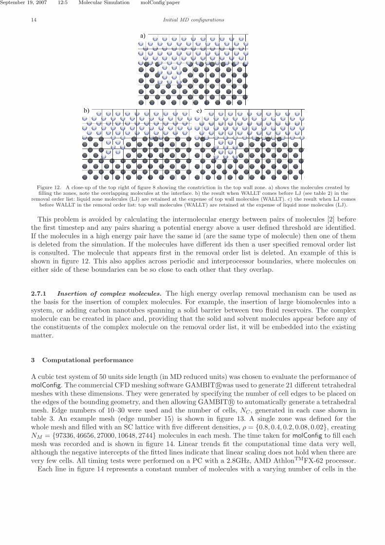
Figure 12. A close-up of the top right of figure 8 showing the constriction in the top wall zone. a) shows the molecules created byfilling the zones, note the overlapping molecules at the interface. b) the result when WALLT comes before LJ (see table 2) in the

removal order list: liquid zone molecules (LJ) are retained at the expense of top wall molecules (WALLT). c) the result when LJ comesbefore WALLT in the removal order list: top wall molecules (WALLT) are retained at the expense of liquid zone molecules (LJ).

This problem is avoided by calculating the intermolecular energy between pairs of molecules [2] beforethe first timestep and any pairs sharing a potential energy above a user defined threshold are identified.If the molecules in a high energy pair have the same id (are the same type of molecule) then one of themis deleted from the simulation. If the molecules have different ids then a user specified removal order listis consulted. The molecule that appears first in the removal order list is deleted. An example of this isshown in figure 12. This also applies across periodic and interprocessor boundaries, where molecules oneither side of these boundaries can be so close to each other that they overlap.

2.7.1 Insertion of complex molecules. The high energy overlap removal mechanism can be used asthe basis for the insertion of complex molecules. For example, the insertion of large biomolecules into asystem, or adding carbon nanotubes spanning a solid barrier between two fluid reservoirs. The complexmolecule can be created in place and, providing that the solid and solvent molecules appear before any ofthe constituents of the complex molecule on the removal order list, it will be embedded into the existingmatter.

3 Computational performance

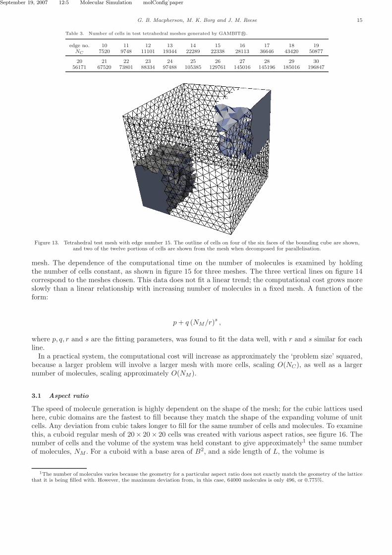
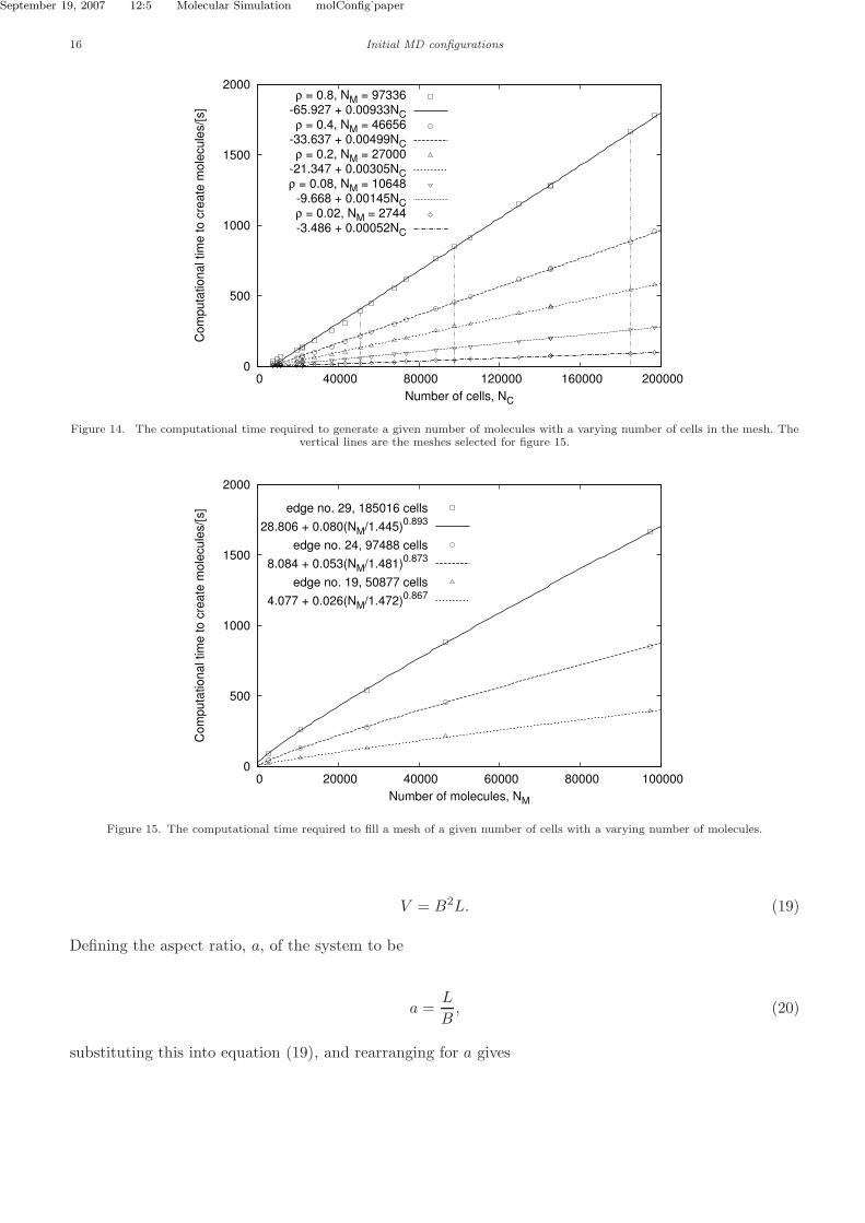
A cubic test system of 50 units side length (in MD reduced units) was chosen to evaluate the performance ofmolConfig. The commercial CFD meshing software GAMBIT R©was used to generate 21 different tetrahedralmeshes with these dimensions. They were generated by specifying the number of cell edges to be placed onthe edges of the bounding geometry, and then allowing GAMBIT R© to automatically generate a tetrahedralmesh. Edge numbers of 10–30 were used and the number of cells, NC , generated in each case shown intable 3. An example mesh (edge number 15) is shown in figure 13. A single zone was defined for thewhole mesh and filled with an SC lattice with five different densities, ρ = {0.8, 0.4, 0.2, 0.08, 0.02}, creatingNM = {97336, 46656, 27000, 10648, 2744} molecules in each mesh. The time taken for molConfig to fill eachmesh was recorded and is shown in figure 14. Linear trends fit the computational time data very well,although the negative intercepts of the fitted lines indicate that linear scaling does not hold when there arevery few cells. All timing tests were performed on a PC with a 2.8GHz, AMD AthlonTMFX-62 processor.

Each line in figure 14 represents a constant number of molecules with a varying number of cells in the



Table 3. Number of cells in test tetrahedral meshes generated by GAMBIT R©.

edge no. 10 11 12 13 14 15 16 17 18 19NC 7520 9748 11101 19344 22289 22338 28113 36646 43420 50877

20 21 22 23 24 25 26 27 28 29 3056171 67520 73801 88334 97488 105385 129761 145016 145196 185016 196847

Figure 13. Tetrahedral test mesh with edge number 15. The outline of cells on four of the six faces of the bounding cube are shown,and two of the twelve portions of cells are shown from the mesh when decomposed for parallelisation.

mesh. The dependence of the computational time on the number of molecules is examined by holdingthe number of cells constant, as shown in figure 15 for three meshes. The three vertical lines on figure 14correspond to the meshes chosen. This data does not fit a linear trend; the computational cost grows moreslowly than a linear relationship with increasing number of molecules in a fixed mesh. A function of theform:

p+ q (NM/r)s ,

where p, q, r and s are the fitting parameters, was found to fit the data well, with r and s similar for eachline.

In a practical system, the computational cost will increase as approximately the ‘problem size’ squared,because a larger problem will involve a larger mesh with more cells, scaling O(NC), as well as a largernumber of molecules, scaling approximately O(NM ).

3.1 Aspect ratio

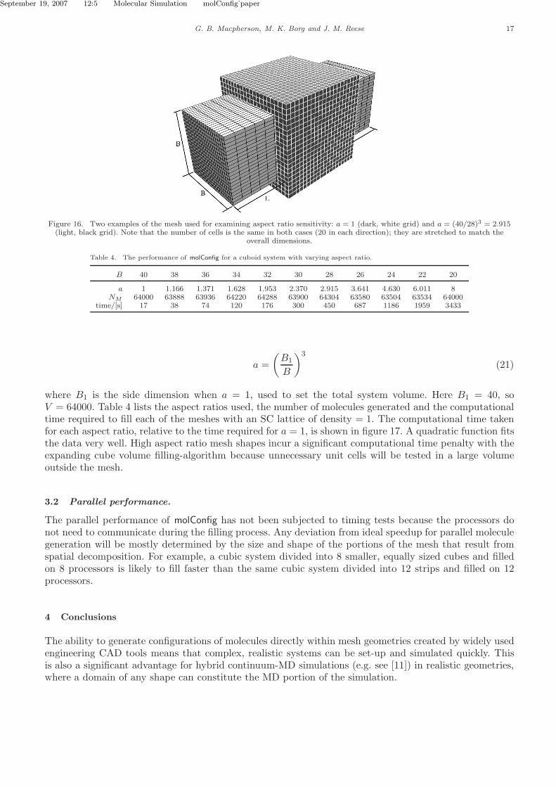
The speed of molecule generation is highly dependent on the shape of the mesh; for the cubic lattices usedhere, cubic domains are the fastest to fill because they match the shape of the expanding volume of unitcells. Any deviation from cubic takes longer to fill for the same number of cells and molecules. To examinethis, a cuboid regular mesh of 20× 20× 20 cells was created with various aspect ratios, see figure 16. Thenumber of cells and the volume of the system was held constant to give approximately1 the same numberof molecules, NM . For a cuboid with a base area of B2, and a side length of L, the volume is

1The number of molecules varies because the geometry for a particular aspect ratio does not exactly match the geometry of the latticethat it is being filled with. However, the maximum deviation from, in this case, 64000 molecules is only 496, or 0.775%.



0

500

1000

1500

2000

0 40000 80000 120000 160000 200000

Co

mp

uta

tio

na

l tim

e t

o c

rea

te m

ole

cu

les/[

s]

Number of cells, NC

ρ = 0.8, NM = 97336-65.927 + 0.00933NC

ρ = 0.4, NM = 46656-33.637 + 0.00499NC

ρ = 0.2, NM = 27000-21.347 + 0.00305NCρ = 0.08, NM = 10648

-9.668 + 0.00145NCρ = 0.02, NM = 2744-3.486 + 0.00052NC

Figure 14. The computational time required to generate a given number of molecules with a varying number of cells in the mesh. Thevertical lines are the meshes selected for figure 15.

0

500

1000

1500

2000

0 20000 40000 60000 80000 100000

Co

mp

uta

tio

na

l tim

e t

o c

rea

te m

ole

cu

les/[

s]

Number of molecules, NM

edge no. 29, 185016 cells

28.806 + 0.080(NM/1.445)0.893


8.084 + 0.053(NM/1.481)0.873


4.077 + 0.026(NM/1.472)0.867

Figure 15. The computational time required to fill a mesh of a given number of cells with a varying number of molecules.

V = B2L. (19)

Defining the aspect ratio, a, of the system to be

a =L

B, (20)

substituting this into equation (19), and rearranging for a gives



Figure 16. Two examples of the mesh used for examining aspect ratio sensitivity: a = 1 (dark, white grid) and a = (40/28)3 = 2.915(light, black grid). Note that the number of cells is the same in both cases (20 in each direction); they are stretched to match the

overall dimensions.

Table 4. The performance of molConfig for a cuboid system with varying aspect ratio.

B 40 38 36 34 32 30 28 26 24 22 20

a 1 1.166 1.371 1.628 1.953 2.370 2.915 3.641 4.630 6.011 8NM 64000 63888 63936 64220 64288 63900 64304 63580 63504 63534 64000

time/[s] 17 38 74 120 176 300 450 687 1186 1959 3433

a =

(

B1

B

)3

(21)

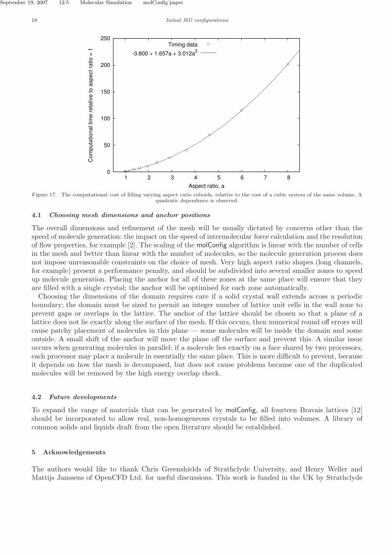
where B1 is the side dimension when a = 1, used to set the total system volume. Here B1 = 40, soV = 64000. Table 4 lists the aspect ratios used, the number of molecules generated and the computationaltime required to fill each of the meshes with an SC lattice of density = 1. The computational time takenfor each aspect ratio, relative to the time required for a = 1, is shown in figure 17. A quadratic function fitsthe data very well. High aspect ratio mesh shapes incur a significant computational time penalty with theexpanding cube volume filling-algorithm because unnecessary unit cells will be tested in a large volumeoutside the mesh.

3.2 Parallel performance.

The parallel performance of molConfig has not been subjected to timing tests because the processors donot need to communicate during the filling process. Any deviation from ideal speedup for parallel moleculegeneration will be mostly determined by the size and shape of the portions of the mesh that result fromspatial decomposition. For example, a cubic system divided into 8 smaller, equally sized cubes and filledon 8 processors is likely to fill faster than the same cubic system divided into 12 strips and filled on 12processors.

4 Conclusions

The ability to generate configurations of molecules directly within mesh geometries created by widely usedengineering CAD tools means that complex, realistic systems can be set-up and simulated quickly. Thisis also a significant advantage for hybrid continuum-MD simulations (e.g. see [11]) in realistic geometries,where a domain of any shape can constitute the MD portion of the simulation.



0

50

100

150

200

250

1 2 3 4 5 6 7 8

Co

mp

uta

tio

na

l tim

e r

ela

tive

to

asp

ect

ratio

= 1

Aspect ratio, a

Timing data

-3.800 + 1.657a + 3.012a2

Figure 17. The computational cost of filling varying aspect ratio cuboids, relative to the cost of a cubic system of the same volume. Aquadratic dependence is observed.

4.1 Choosing mesh dimensions and anchor positions

The overall dimensions and refinement of the mesh will be usually dictated by concerns other than thespeed of molecule generation: the impact on the speed of intermolecular force calculation and the resolutionof flow properties, for example [2]. The scaling of the molConfig algorithm is linear with the number of cellsin the mesh and better than linear with the number of molecules, so the molecule generation process doesnot impose unreasonable constraints on the choice of mesh. Very high aspect ratio shapes (long channels,for example) present a performance penalty, and should be subdivided into several smaller zones to speedup molecule generation. Placing the anchor for all of these zones at the same place will ensure that theyare filled with a single crystal; the anchor will be optimised for each zone automatically.

Choosing the dimensions of the domain requires care if a solid crystal wall extends across a periodicboundary; the domain must be sized to permit an integer number of lattice unit cells in the wall zone toprevent gaps or overlaps in the lattice. The anchor of the lattice should be chosen so that a plane of alattice does not lie exactly along the surface of the mesh. If this occurs, then numerical round off errors willcause patchy placement of molecules in this plane — some molecules will be inside the domain and someoutside. A small shift of the anchor will move the plane off the surface and prevent this. A similar issueoccurs when generating molecules in parallel: if a molecule lies exactly on a face shared by two processors,each processor may place a molecule in essentially the same place. This is more difficult to prevent, becauseit depends on how the mesh is decomposed, but does not cause problems because one of the duplicatedmolecules will be removed by the high energy overlap check.

4.2 Future developments

To expand the range of materials that can be generated by molConfig, all fourteen Bravais lattices [12]should be incorporated to allow real, non-homogeneous crystals to be filled into volumes. A library ofcommon solids and liquids draft from the open literature should be established.

5 Acknowledgements

The authors would like to thank Chris Greenshields of Strathclyde University, and Henry Weller andMattijs Janssens of OpenCFD Ltd. for useful discussions. This work is funded in the UK by Strathclyde


REFERENCES 19

University, the Miller Foundation and the James Weir Foundation, and through a Philip Leverhulme Prizefor JMR from the Leverhulme Trust.

References

[1] OpenFOAM: The Open Source CFD Toolbox. http://www.openfoam.org.[2] Graham B. Macpherson and Jason M. Reese. Molecular dynamics in arbitrary geometries: parallel

evaluation of pair forces. Submitted to Molecular Simulation, 2007.[3] J. G. Powles, S. Murad, and P. V. Ravi. A new model for permeable micropores. Chemical Physics

Letters, 188:21–24, 1992.[4] K.P. Travis, B.D. Todd, and D.J. Evans. Departure from Navier-Stokes hydrodynamics in confined

liquids. Physical Review E, 55(4):4288–95, 1997.[5] Herbert Goldstein. Classical Mechanics. Addison-Wesley, 2nd edition, 1980.[6] D. C. Rapaport. The Art of Molecular Dynamics Simulation. Cambridge University Press, 2nd

edition, 2004.[7] M.P. Allen and D.J. Tildesley. Computer simulation of liquids. Oxford University Press, 1987.[8] George Karypis and Vipin Kumar. METIS. A software package for partitioning unstructured graphs,

partitioning meshes, and computing fill-reducing orderings of sparse matrices. Version 4.0. Universityof Minnesota, http://glaros.dtc.umn.edu/gkhome/views/metis.

[9] ParaView: Parallel Visualization Application. http://www.paraview.org.[10] L. D. Landau and E. M. Lifshitz. Statistical Physics Part 1 (Course of Theoretical Physics v.5).

Pergamon, 3rd edition, 1980.[11] Thomas Werder, Jens H. Walther, and Petros Koumoutsakos. Hybrid atomistic-continuum method

for the simulation of dense fluid flows. Journal of Computational Physics, 205(1):373–390, 2005.[12] Charles Kittel. Introduction to solid state physics. Wiley, 8th edition, 2005.

Documents

Generation of initial molecular dynamics conﬁgurations in ... · September 19, 2007 12:5 Molecular Simulation molConﬁg˙paper Molecular Simulation, Vol. 00, No. 00, DD Month 200x,