Generalized Singular Value Thresholding

Canyi Lu1, Changbo Zhu1, Chunyan Xu2, Shuicheng Yan1, Zhouchen Lin3,∗1 Department of Electrical and Computer Engineering, National University of Singapore

2 School of Computer Science and Technology, Huazhong University of Science and Technology3 Key Laboratory of Machine Perception (MOE), School of EECS, Peking University

canyilu@nus.edu.sg, zhuchangbo@gmail.com, xuchunyan01@gmail.com, eleyans@nus.edu.sg, zlin@pku.edu.cn

AbstractThis work studies the Generalized Singular ValueThresholding (GSVT) operator Proxσ

g (·),

Proxσg (B) = argmin

X

m∑i=1

g(σi(X))+1

2||X−B||2F ,

associated with a nonconvex function g defined on thesingular values of X. We prove that GSVT can be ob-tained by performing the proximal operator of g (denot-ed as Proxg(·)) on the singular values since Proxg(·)is monotone when g is lower bounded. If the noncon-vex g satisfies some conditions (many popular noncon-vex surrogate functions, e.g., `p-norm, 0 < p < 1,of `0-norm are special cases), a general solver to findProxg(b) is proposed for any b ≥ 0. GSVT great-ly generalizes the known Singular Value Thresholding(SVT) which is a basic subroutine in many convex lowrank minimization methods. We are able to solve thenonconvex low rank minimization problem by usingGSVT in place of SVT.

IntroductionThe sparse and low rank structures have received much at-tention in recent years. There have been many applicationswhich exploit these two structures, such as face recognition(Wright et al. 2009), subspace clustering (Cheng et al. 2010;Liu et al. 2013b) and background modeling (Candes et al.2011). To achieve sparsity, a principled approach is to usethe convex `1-norm. However, the `1-minimization may besuboptimal, since the `1-norm is a loose approximation ofthe `0-norm and often leads to an over-penalized problem.This brings the attention back to the nonconvex surrogate byinterpolating the `0-norm and `1-norm. Many nonconvex pe-nalities have been proposed, including `p-norm (0 < p < 1)(Frank and Friedman 1993), Smoothly Clipped AbsoluteDeviation (SCAD) (Fan and Li 2001), Logarithm (Friedman2012), Minimax Concave Penalty (MCP) (Zhang and others2010), Geman (Geman and Yang 1995) and Laplace (Trza-sko and Manduca 2009). Their definitions are shown in Ta-ble 1. Numerical studies (Candes, Wakin, and Boyd 2008)have shown that the nonconvex optimization usually outper-forms convex models.

∗Corresponding author.Copyright c© 2015, Association for the Advancement of ArtificialIntelligence (www.aaai.org). All rights reserved.

Table 1: Popular nonconvex surrogate functions of `0-norm(||θ||0).

Penalty Formula g(θ), θ ≥ 0, λ > 0`p-norm λθp, 0 < p < 1.

SCAD

λθ, if θ ≤ λ,−θ2+2γλθ−λ2

2(γ−1), if λ < θ ≤ γλ,

λ2(γ+1)2

, if θ > γλ.

Logarithm λlog(γ+1)

log(γθ + 1)

MCP

λθ − θ2

2γ, if θ < γλ,

12γλ2, if θ ≥ γλ.

Geman λθθ+γ

.Laplace λ(1− exp(− θ

γ)).

The low rank structure is an extension of sparsity definedon the singular values of a matrix. A principled way is touse the nuclear norm which is a convex surrogate of therank function (Recht, Fazel, and Parrilo 2010). However, itsuffers from the same suboptimal issue as the `1-norm inmany cases. Very recently, many popular nonconvex surro-gate functions in Table 1 are extended on the singular val-ues to better approximate the rank function (Lu et al. 2014).However, different from the convex optimization, the non-convex low rank minimization is much more challengingthan the nonconvex sparse minimization.

The Iteratively Reweighted Nuclear Norm (IRNN)method is proposed to solve the following nonconvex lowrank minimization problem (Lu et al. 2014)

minX

F (X) =

m∑i=1

g(σi(X)) + h(X), (1)

where σi(X) denotes the i-th singular value of X ∈ Rm×n(we assume m ≤ n in this work). g : R+ → R+ is contin-uous, concave and nonincreasing on [0,+∞). Popular non-convex surrogate functions in Table 1 are some examples.h : Rm×n → R+ is the loss function which has Lipschitzcontinuous gradient. IRNN updates Xk+1 by minimizing asurrogate function which upper bounds the objective func-tion in (1). The surrogate function is constructed by lineariz-ing g and h at Xk, simultaneously. In theory, IRNN guaran-tees to decrease the objective function value of (1) in eachiteration. However, it may decrease slowly since the upper

0 2 4 60

2

4

6

θ

Gra

dien

t ∇ g

(θ)

(a) `p-norm

0 2 4 60

0.5

1

θ

Gra

dien

t ∇ g

(θ)

(b) SCAD

0 2 4 60

0.5

1

1.5

θ

Gra

dien

t ∇ g

(θ)

(c) Logarithm

0 2 4 60

0.5

1

θ

Gra

dien

t ∇ g

(θ)

(d) MCP

0 2 4 60

0.5

1

θ

Gra

dien

t ∇ g

(θ)

(e) Geman

0 2 4 60

0.5

1

θ

Gra

dien

t ∇ g

(θ)

(f) Laplace

Figure 1: Gradients of some nonconvex functions (For `p-norm, p = 0.5. For all penalties, λ = 1, γ = 1.5).

bound surrogate may be quite loose. It is expected that min-imizing a tighter surrogate will lead to a faster convergence.

A possible tighter surrogate function of the objectivefunction in (1) is to keep g and relax h only. This leads tothe following updating rule which is named as GeneralizedProximal Gradient (GPG) method in this work

Xk+1 = arg minX

m∑i=1

g(σi(X)) + h(Xk)

+ 〈∇h(Xk),X−Xk〉+µ

2||X−Xk||2F

= arg minX

m∑i=1

g(σi(X)) +µ

2||X−Xk +

1

µ∇h(Xk)||2F ,

(2)where µ > L(h), L(h) is the Lipschitz constant of h, guar-antees the convergence of GPG as shown later. It can be seenthat solving (2) requires solving the following problem

Proxσg (B) = arg minX

m∑i=1

g(σi(X)) +1

2||X−B||2F . (3)

In this work, the mapping Proxσg (·) is called the Gener-alized Singular Value Thresholding (GSVT) operator asso-ciated with the function

∑mi=1 g(·) defined on the singular

values. If g(x) = λx,∑mi=1 g(σi(X)) is degraded to the

convex nuclear norm λ||X||∗. Then (3) has a closed for-m solution Proxσg (B) = UDiag(Dλ(σ(B)))VT , whereDλ(σ(B)) = (σi(B) − λ)+mi=1, and U and V are fromthe SVD of B, i.e., B = UDiag(σ(B))VT . This is theknown Singular Value Thresholding (SVT) operator associ-ated with the convex nuclear norm (when g(x) = λx) (Cai,Candes, and Shen 2010). More generally, for a convex g, thesolution to (3) is

Proxσg (B) = UDiag(Proxg(σ(B)))VT , (4)

where Proxg(·) is defined element-wise as follows,

Proxg(b) = arg minx≥0

fb(x) = g(x) +1

2(x− b)2, 1 (5)

1For x < 0, g(x) = g(−x). If b ≥ 0, Proxg(b) ≥ 0. If b < 0,Proxg(b) = −Proxg(−b). So we only need to discuss the caseb, x ≥ 0 in this work.

where Proxg(·) is the known proximal operator associat-ed with a convex g (Combettes and Pesquet 2011). That isto say, solving (3) is equivalent to performing Proxg(·) oneach singular value of B. In this case, the mapping Proxg(·)is unique, i.e., (5) has a unique solution. More importantly,Proxg(·) is monotone, i.e., Proxg(x1) ≥ Proxg(x2) forany x1 ≥ x2. This guarantees to preserve the nonincreasingorder of the singular values after shrinkage and threshold-ing by the mapping Proxg(·). For a nonconvex g, we stillcall Proxg(·) as the proximal operator, but note that sucha mapping may not be unique. It is still an open problemwhether Proxg(·) is monotone or not for a nonconvex g.Without proving the monotonity of Proxg(·), one cannotsimply perform it on the singular values of B to obtain thesolution to (3) as SVT. Even if Proxg(·) is monotone, sinceit is not unique, one also needs to carefully choose the solu-tion pi ∈ Proxg(σi(B)) such that p1 ≥ p2 ≥ · · · ≥ pm.Another challenging problem is that there does not exist ageneral solver to (5) for a general nonconvex g.

It is worth mentioning that some previous works stud-ied the solution to (3) for some special choices of non-convex g (Nie, Huang, and Ding 2012; Chartrand 2012;Liu et al. 2013a). However, none of their proofs was rig-orous since they ignored proving the monotone property ofProxg(·). See the detailed discussions in the next section.Another recent work (Gu et al. 2014) considered the follow-ing problem related to the weighted nuclear norm:

minX

fw,B(X) =

m∑i=1

wiσi(X) +1

2||X−B||2F , (6)

where wi ≥ 0, i = 1, · · · ,m. Problem (6) is a little moregeneral than (3) by taking different gi(x) = wix. It isclaimed in (Gu et al. 2014) that the solution to (6) isX∗ = UDiag (Proxgi(σi(B)), i = 1, · · · ,m)VT , (7)

where B = UDiag(σ(B))VT is the SVD of B, andProxgi(σi(B)) = maxσi(B) − wi, 0. However, such aresult and their proof are not correct. A counterexample isas follows:

B =

[0.0941 0.42010.5096 0.0089

], w =

[0.50.25

],

X∗ =

[−0.0345 0.12870.0542 −0.0512

], X =

[0.0130 0.19380.1861 −0.0218

],

where X∗ is obtained by (7). The solution X∗ is not op-timal to (6) since there exists X shown above such thatfw,B(X) = 0.2262 < fw,B(X∗) = 0.2393. The reasonbehind is that(Prox gi(σi(B))−Prox gj (σj(B)))(σi(B)−σj(B)) ≥ 0,

(8)does not guarantee to hold for any i 6= j. Note that (8) holdswhen 0 ≤ w1 ≤ · · · ≤ wm, and thus (7) is optimal to (6) inthis case.

In this work, we give the first rigorous proof thatProxg(·) is monotone for any lower bounded function (re-gardless of the convexity of g). Then solving (3) is degener-ated to solving (5) for each b = σi(B). The Generalized Sin-gular Value Thresholding (GSVT) operator Proxσg (·) asso-ciated with any lower bounded function in (3) is much more

general than the known SVT associated with the convex nu-clear norm (Cai, Candes, and Shen 2010). In order to com-pute GSVT, we analyze the solution to (5) for certain typesof g (some special cases are shown in Table 1) in theory, andpropose a general solver to (5). At last, with GSVT, we cansolve (1) by the Generalized Proximal Gradient (GPG) al-gorithm shown in (2). We test both Iteratively ReweightedNuclear Norm (IRNN) and GPG on the matrix completionproblem. Both synthesis and real data experiments show thatGPG outperforms IRNN in terms of the recovery error andthe objective function value.

Generalized Singular Value ThresholdingProblem ReformulationA main goal of this work is to compute GSVT (3), and usesit to solve (1). We will show that, if Proxg(·) is monotone,problem (3) can be reformulated into an equivalent problemwhich is much easier to solve.Lemma 1. (von Neumann’s trace inequality (Rhea 2011))For any matrices A, B ∈ Rm×n (m ≤ n), Tr(ATB) ≤∑mi=1 σi(A)σi(B), where σ1(A) ≥ σ2(A) ≥ · · · ≥ 0 and

σ1(B) ≥ σ2(B) ≥ · · · ≥ 0 are the singular values of Aand B, respectively. The equality holds if and only if thereexist unitaries U and V such that A = UDiag(σ(A))VT

and B = UDiag(σ(B))VT are the SVDs of A and B,simultaneously.Theorem 1. Let g : R+ → R+ be a function such thatProxg(·) is monotone. Let B = UDiag(σ(B))VT be theSVD of B ∈ Rm×n. Then an optimal solution to (3) is

X∗ = UDiag(%∗)VT , (9)

where %∗ satisfies %∗1 ≥ %∗2 ≥ · · · ≥ %∗m, i = 1, · · · ,m, and

%∗i ∈ Proxg(σi(B)) = argmin%i≥0

g(%i) +1

2(%i − σi(B))2.

(10)

Proof. Denote σ1(X) ≥ · · · ≥ σm(X) ≥ 0 as the singularvalues of X. Problem (3) can be rewritten as

min%:%1≥···≥%m≥0

min

σ(X)=%

m∑i=1

g(%i) +1

2||X−B||2F

.

(11)By using the von Neumann’s trace inequality in Lemma 1,we have

||X−B||2F = Tr (XTX)− 2 Tr(XTB) + Tr(BTB)

=

m∑i=1

σ2i (X)− 2 Tr(XTB) +

m∑i=1

σ2i (B)

≥m∑i=1

σ2i (X)− 2

m∑i=1

σi(X)σi(B) +

m∑i=1

σ2i (B)

=

m∑i=1

(σi(X)− σi(B))2.

Note that the above equality holds when X admits the sin-gular value decomposition X = UDiag(σ(X))VT , where

U and V are the left and right orthonormal matrices in theSVD of B. In this case, problem (11) is reduced to

min%:%1≥···≥%m≥0

m∑i=1

(g(%i) +

1

2(%i − σi(B))2

). (12)

Since Proxg(·) is monotone and σ1(B) ≥ σ2(B) ≥ · · · ≥σm(B), there exists %∗i ∈ Proxg(σi(B)), such that %∗1 ≥%∗2 ≥ · · · ≥ %∗m. Such a choice of %∗ is optimal to (12), andthus (9) is optimal to (3).

From the above proof, it can be seen that the monotoneproperty of Proxg(·) is a key condition which makes prob-lem (12) separable conditionally. Thus the solution (9) to(3) shares a similar formulation as the known Singular Val-ue Thresholding (SVT) operator associated with the convexnuclear norm (Cai, Candes, and Shen 2010). Note that for aconvex g, Proxg(·) is always monotone. Indeed,

(Prox g(b1)−Prox g(b2)) (b1 − b2)

≥ (Proxg(b1)−Proxg(b2))2 ≥ 0, ∀ b1, b2 ∈ R+.

The above inequality can be obtained by the optimality ofProxg(·) and the convexity of g.

The monotonicity of Proxg(·) for a nonconvex g is stil-l unknown. There were some previous works (Nie, Huang,and Ding 2012; Chartrand 2012; Liu et al. 2013a) claimingthat the solution (9) is optimal to (3) for some special choicesof nonconvex g. However, their results are not rigorous sincethe monotone property of Proxg(·) is not proved. Surpris-ingly, we find that the monotone property of Proxg(·) holdsfor any lower bounded function g.Theorem 2. For any lower bounded function g, its prox-imal operator Proxg(·) is monotone, i.e., for any p∗i ∈Proxg(xi), i = 1, 2, p∗1 ≥ p∗2, when x1 > x2.

Note that it is possible that σi(B) = σj(B) for some i <j in (10). Since Proxg(·) may not be unique, we need tochoose %∗i ∈ Proxg(σi(B)) and %∗j ∈ Proxg(σj(B)) suchthat %∗i ≤ %∗j . This is the only difference between GSVT andSVT.

Proximal Operator of Nonconvex FunctionSo far, we have proved that solving (3) is equivalent to solv-ing (5) for each b = σi(B), i = 1, · · · ,m, for any lowerbounded function g. For a nonconvex g, only for some spe-cial cases, the candidate solutions to (5) have a closed form(Gong et al. 2013). There does not exist a general solver fora more general nonconvex g. In this section, we analyze thesolution to (5) for a broad choice of the nonconvex g. Thena general solver will be proposed in the next section.Assumption 1. g : R+ → R+, g(0) = 0. g is concave, non-decreasing and differentiable. The gradient∇g is convex.

In this work, we are interested in the nonconvex surrogateof `0-norm. Except the differentiablity of g and the convexi-ty of∇g, all the other assumptions in Assumption 1 are nec-essary for constructing a surrogate of `0-norm. As we willsee later, these two additional assumptions make our analy-sis much easier. Note that the assumptions for the noncon-vex function considered in Assumption 1 are quite general.

Algorithm 1: A General Solver to (5) in which g satisfyingAssumption 1

Input: b ≥ 0.Output: Identify an optimal solution, 0 or

xb = maxx|∇fb(x) = 0, 0 ≤ x ≤ b.if∇g(b) = 0 then

return xb = b;else

// find xb by fixed point iteration.x0 = b. // Initialization.while not converge do

xk+1 = b−∇g(xk);if xk+1 < 0 then

return xb = 0;break;

endend

endCompare fb(0) and fb(xb) to identify the optimal one.

It is easy to verify that many popular surrogate functions of`0-norm shown in Table 1 satisfy Assumption 1, including`p-norm, Logarithm, MCP, Geman and Laplace penalties.Only the SCAD penalty violates the convex∇g assumption,as shown in Figure 1.Proposition 1. Given g satisfying Assumption 1, the opti-mal solution to (5) lies in [0, b].

The above fact is obvious since both g(x) and 12 (x − b)2

are nondecreasing on [b,+∞). Such a result limits the so-lution space, and thus is very useful for our analysis. Ourgeneral solver to (5) is also based on Proposition 1.

Note that the solutions to (5) lie in 0 or the localpoints x|∇fb(x) = ∇g(x) + x − b = 0. Our analy-sis is mainly based on the number of intersection pointsof D(x) = ∇g(x) and the line Cb(x) = b − x. Letb = supb | Cb(x) and D(x) have no intersection. Wehave the solution to (5) in different cases. Please refer to thesupplementary material for the detailed proofs.Proposition 2. Given g satisfying Assumption 1 and∇g(0) = +∞. Restricted on [0,+∞), when b > b, Cb(x)and D(x) have two intersection points, denoted as P b1 =(xb1, y

b1), P b2 = (xb2, y

b2), and xb1 < xb2. If there does not exist

b > b such that fb(0) = fb(xb2), then Proxg(b) = 0 for all

b ≥ 0. If there exists b > b such that fb(0) = fb(xb2), let

b∗ = infb | fb(0) = fb(xb2) . Then we have

Proxg(b) = argminx≥0

fb(x)

= xb2, if b > b∗,3 0, if b ≤ b∗.

Proposition 3. Given g satisfying Assumption 1 and∇g(0) < +∞. Restricted on [0,+∞), if we haveC∇g(0)(x) = ∇g(0) − x ≤ ∇g(x) for all x ∈ (0,∇g(0)),then Cb(x) and D(x) have only one intersection point(xb, yb) when b > ∇g(0). Furthermore,

Proxg(b) = argminx≥0

fb(x)

= xb, if b > ∇g(0),3 0, if b ≤ ∇g(0).

0 0.5 1 1.5 2 2.5 30

0.2

0.4

0.6

0.8

1

1.2

1.4

1.6

1.8

2l1

b

Pro

x g(b)

(a) `1-norm

0 0.5 1 1.5 2 2.5 30

0.5

1

1.5

2

2.5

3lp

b

Pro

x g(b)

(b) `p-norm

0 0.5 1 1.5 2 2.5 30

0.5

1

1.5

2

2.5

3mcp

b

Pro

x g(b)

(c) MCP

0 0.5 1 1.5 2 2.5 30

0.5

1

1.5

2

2.5

3logarithm

b

Pro

x g(b)

(d) Logarithm

0 0.5 1 1.5 2 2.5 30

0.5

1

1.5

2

2.5

3laplace

b

Pro

x g(b)

(e) Laplace

0 0.5 1 1.5 2 2.5 30

0.5

1

1.5

2

2.5

3geman

b

Pro

x g(b)

(f) Geman

Figure 2: Plots of b v.s. Proxg(b) for different choices ofg: convex `1-norm and popular nonconvex functions whichsatisfy Assumption 1 in Table 1.

Suppose there exists 0 < x < ∇g(0) such that C∇g(0)(x) =

∇g(0) − x > ∇g(x). Then, when ∇g(0) ≥ b > b, Cb(x)andD(x) have two intersection points, which are denoted asP b1 = (xb1, y

b1) and P b2 = (xb2, y

b2) such that xb1 < xb2. When

∇g(0) < b, Cb(x) and D(x) have only one intersectionpoint (xb, yb). Also, there exists b such that ∇g(0) > b > band fb(0) = fb(x

b2). Let b∗ = infb | fb(0) = fb(x

b2) . We

have

Proxg(b) = argminx≥0

fb(x)

= xb, if b > ∇g(0),= xb2, if ∇g(0) ≥ b > b∗,3 0, if b ≤ b∗.

Corollary 1. Given g satisfying Assumption 1. Denotexb = maxx|∇fb(x) = 0, 0 ≤ x ≤ b and x∗ =arg minx∈0,xb fb(x). Then x∗ is optimal to (5).

The results in Proposition 2 and 3 give the solution to (5)in different cases, while Corollary 1 summarizes these re-sults. It can be seen that one only needs to compute xb whichis the largest local minimum. Then comparing the objectivefunction value at 0 and xb leads to an optimal solution to (5).

AlgorithmsIn this section, we first give a general solver to (5) in which gsatisfies Assumption 1. Then we are able to solve the GSVTproblem (3). With GSVT, problem (1) can be solved by Gen-eralized Proximal Gradient (GPG) algorithm as shown in(2). We also give the convergence guarantee of GPG.

A General Solver to (5)Given g satisfying Assumption 1, as shown in Corollary 1,0 and xb = maxx|∇fb(x) = 0, 0 ≤ x ≤ b are the can-didate solutions to (5). The left task is to find xb which isthe largest local minimum point near x = b. So we can startsearching for xb from x0 = b by the fixed point iterationalgorithm. Note that it will be very fast since we only needto search within [0, b]. The whole procedure to find xb can

20 22 24 26 28 30 32 340

0.1

0.2

0.3

0.4

0.5

0.6

0.7

0.8

0.9

1

Rank

Freq

uenc

y of

Suc

ess

ALMIRNNGPG

(a)

15 20 25 300

0.05

0.1

0.15

0.2

0.25

0.3

0.35

0.4

0.45

Rank

Rel

ativ

e E

rror

APGLIRNNGPG

(b)

0 10 20 30 40 500

2

4

6

8

10 x 104

Iteration

Obj

ectiv

e fu

nctio

n va

lue

Rank = 15

0 10 20 30 40 502

4

6

8

10

12 x 104

Iteration

Obj

ectiv

e fu

nctio

n va

lue

Rank = 20

0 10 20 30 40 500

5

10

15 x 104

Iteration

Obj

ectiv

e fu

nctio

n va

lue

Rank = 25

0 10 20 30 40 500

0.5

1

1.5

2 x 105

Iteration

Obj

ectiv

e fu

nctio

n va

lue

Rank = 30

IRNNGPG

IRNNGPG

IRNNGPG

IRNNGPG

(c)Figure 3: Experimental results of low rank matrix recovery on random data. (a) Frequency of Success (FoS) for a noise freecase. (b) Relative error for a noisy case. (c) Convergence curves of IRNN and GPG for a noisy case.

be found in Algorithm 1. In theory, it can be proved that thefixed point iteration guarantees to find xb. Please refer to thesupplementary material for the detailed proof.

If g is nonsmooth or ∇g is nonconvex, the fixed pointiteration algorithm may also be applicable. The key is to findall the local solutions with smart initial points. Also all thenonsmooth points should be considered as the candidates.

All the nonconvex surrogates g except SCAD in Table 1satisfy Assumption 1, and thus the solution Proxg(b) to(5) can be obtained by Algorithm 1. Figure 2 illustrates theshrinkage effect of proximal operators of these functions andthe convex `1-norm. The shrinkage and thresholding effectof these proximal operators are similar when b is relative-ly small. However, when b is relatively large, the proximaloperators of the nonconvex functions are nearly unbiased,i.e., keeping b nearly the same as the `0-norm. On the con-trast, the proximal operator of the convex `1-norm is biased.In this case, the `1-norm may be over-penalized, and thusmay perform quite differently from the `0-norm. This alsosupports the necessity of using nonconvex penalties on thesingular values to approximate the rank function.

Generalized Proximal Gradient Algorithm for (1)Given g satisfying Assumption 1, we are now able to getthe optimal solution to (3) by (9) and Algorithm 1. Now wehave a better solver than IRNN to solve (1) by the updatingrule (2), or equivalently

Xk+1 = Proxσ1µ g

(Xk − 1

µ∇h(Xk)

).

The above updating rule is named as Generalized ProximalGradient (GPG) for the nonconvex problem (1). It can be re-garded as a generalization of previous methods (Beck andTeboulle 2009; Gong et al. 2013). The main per-iterationcost of GPG is to compute an SVD. Such per-iteration com-plexity is the same as many convex methods (Toh and Yun2010a; Lin, Chen, and Ma 2009). In theory, we have the fol-lowing convergence results for GPG. Please refer to the de-tailed convergence proof in the supplementary material.Theorem 3. If µ > L(h), the sequence Xk generated by(2) satisfies the following properties:(1) F (Xk) is monotonically decreasing.

(2) limk→+∞

(Xk −Xk+1) = 0;

(3) If F (X) → +∞ when ||X||F → +∞, then any limitpoint of Xk is a stationary point.

It is expected that GPG will decrease the objective func-tion value faster than IRNN since it uses a tighter surrogatefunction. This will be verified by the experiments.

ExperimentsIn this section, we conduct some experiments on the matrixcompletion problem to test our proposed GPG algorithm

minX

m∑i=1

g(σi(X)) +1

2||PΩ(X)− PΩ(M)||2F , (13)

where Ω is the index set, and PΩ : Rm×n → Rm×n is a lin-ear operator that keeps the entries in Ω unchanged and thoseoutside Ω zeros. Given PΩ(M), the goal of matrix comple-tion is to recover M which is of low rank. Note that we havemany choices of g which satisfies Assumption 1, and wesimply test on the Logarithm penalty, since it is suggest-ed in (Lu et al. 2014; Candes, Wakin, and Boyd 2008) thatit usually performs well by comparing with other noncon-vex penalties. Problem (13) can be solved by GPG by usingGSVT (9) in each iteration. We compared GPG with IRNNon both synthetic and real data. The continuation techniqueis used to enhance the low rank matrix recovery in GPG. Theinitial value of λ in the Logarithm penalty is set to λ0, anddynamically decreased till reaching λt.

Low-Rank Matrix Recovery on Random DataWe conduct two experiments on synthetic data without andwith noises (Lu et al. 2014). For the noise free case, we gen-erate M = M1M2, where M1 ∈ Rm×r, M2 ∈ Rr×n arei.i.d. random matrices, and m = n = 150. The underlyingrank r varies from 20 to 33. Half of the elements in M aremissing. We set λ0 = 0.9||PΩ(M)||∞, and λt = 10−5λ0.The relative error RelErr= ||X∗ −M||F /||M||F is used toevaluate the recovery performance. If RelErr is smaller than10−3, X∗ is regarded as a successful recovery of M. Werepeat the experiments 100 times for each r. We compareGPG by using GSVT with IRNN and the convex Augment-ed Lagrange Multiplier (ALM) (Lin, Chen, and Ma 2009).

recovered image by APGL

23

24

25

26

27

28

APGL IRNN GPG

PSN

R

0.04

0.06

0.08

0.1

APGL IRNN GPG

Rel

ativ

e Er

ror

(a) Original (b) Noisy (c) APGL (d) IRNN (e) GPG

23

24

25

26

27

28

APGL IRNN GPG

PS

NR

0.04

0.06

0.08

0.1

APGL IRNN GPG

Re

lati

ve

Erro

r

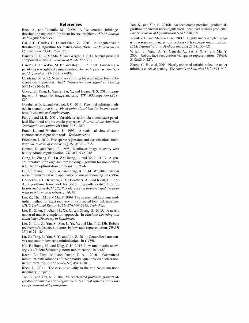
(f) PSNR & errorFigure 4: Image inpainting by APGL, IRNN, and GPG.

Figure 3 (a) plots r v.s. the frequency of success. It can beseen that GPG is slightly better than IRNN when r is rela-tively small, while both IRNN and GPG fail when r ≥ 32.Both of them outperform the convex ALM method, since thenonconvex logarithm penalty approximates the rank func-tion better than the convex nuclear norm.

For the noisy case, the data matrix M is generated inthe same way, but are added some additional noises 0.1E,where E is an i.i.d. random matrix. For this task, we setλ0 = 10||PΩ(M)||∞, and λt = 0.1λ0 in GPG. The con-vex APGL algorithm (Toh and Yun 2010b) is comparedin this task. Each method is run 100 times for each r ∈15, 18, 20, 23, 25, 30. Figure 3 (b) shows the mean relativeerror. It can be seen that GPG by using GSVT in each itera-tion significantly outperforms IRNN and APGL. The reasonis that λt is not that small as in the noise free case. Thus,the upper bound surrogate of g in IRNN will be much moreloose than that in GPG. Figure 3 (c) plots some convergencecurves of GPG and IRNN. It can be seen that GPG withoutrelaxing g will decrease the objective function value faster.

Applications on Real DataMatrix completion can be applied to image inpainting sincethe main information is dominated by the top singular val-ues. For a color image, assume that 40% of pixels are uni-formly missing. They can be recovered by applying low rankmatrix completion on each channel (red, green and blue) ofthe image independently. Besides the relative error definedabove, we also use the Peak Signal-to-Noise Ratio (PSNR)to evaluate the recovery performance. Figure 4 shows twoimages recovered by APGL, IRNN and GPG, respectively.It can be seen that GPG achieves the best performance, i.e.,the largest PSNR value and the smallest relative error.

We also apply matrix completion for collaborative filter-ing. The task of collaborative filtering is to predict the un-known preference of a user on a set of unrated items, ac-cording to other similar users or similar items. We test on theMovieLens data set (Herlocker et al. 1999) which includesthree problems, “movie-100K”, “movie-1M” and “movie-10M”. Since only the entries in Ω of M are known, weuse Normalized Mean Absolute Error (NMAE) ||PΩ(X∗)−

PΩ(M)||1/|Ω| to evaluate the performance as in (Toh andYun 2010b). As shown in Table 2, GPG achieves the bestperformance. The improvement benefits from the GPG al-gorithm which uses a fast and exact solver of GSVT (9).

Table 2: Comparison of NMAE of APGL, IRNN and GPGfor collaborative filtering.

Problem size of M: (m,n) APGL IRNN GPGmoive-100K (943, 1682) 2.76e-3 2.60e-3 2.53e-3moive-1M (6040, 3706) 2.66e-1 2.52e-1 2.47e-1moive-10M (71567, 10677) 3.13e-1 3.01e-1 2.89e-1

ConclusionsThis paper studied the Generalized Singular Value Thresh-olding (GSVT) operator associated with the nonconvexfunction g on the singular values. We proved that the prox-imal operator of any lower bounded function g (denotedas Proxg(·)) is monotone. Thus, GSVT can be obtainedby performing Proxg(·) on the singular values separate-ly. Given b ≥ 0, we also proposed a general solver tofind Proxg(b) for certain type of g. At last, we applied thegeneralized proximal gradient algorithm by using GSVT asthe subroutine to solve the nonconvex low rank minimiza-tion problem (1). Experimental results showed that it out-performed previous method with smaller recovery error andobjective function value.

For nonconvex low rank minimization, GSVT plays thesame role as SVT in convex minimization. One may extendother convex low rank models to nonconvex cases, and solvethem by using GSVT in place of SVT. An interesting fu-ture work is to solve the nonconvex low rank minimizationproblem with affine constraint by ALM (Lin, Chen, and Ma2009) and prove the convergence.

AcknowledgementsThis research is supported by the Singapore National Re-search Foundation under its International Research Centre@Singapore Funding Initiative and administered by the ID-M Programme Office. Z. Lin is supported by NSF of China(Grant nos. 61272341, 61231002, and 61121002) and M-SRA. C. Lu is also supported by the MSRA fellowship 2014.

ReferencesBeck, A., and Teboulle, M. 2009. A fast iterative shrinkage-thresholding algorithm for linear inverse problems. SIAM Journalon Imaging Sciences.Cai, J.-F.; Candes, E. J.; and Shen, Z. 2010. A singular valuethresholding algorithm for matrix completion. SIAM Journal onOptimization 20(4):1956–1982.Candes, E. J.; Li, X.; Ma, Y.; and Wright, J. 2011. Robust principalcomponent analysis? Journal of the ACM 58(3).Candes, E. J.; Wakin, M. B.; and Boyd, S. P. 2008. Enhancing s-parsity by reweighted `1 minimization. Journal of Fourier Analysisand Applications 14(5-6):877–905.Chartrand, R. 2012. Nonconvex splitting for regularized low-rank+sparse decomposition. IEEE Transactions on Signal Processing60(11):5810–5819.Cheng, B.; Yang, J.; Yan, S.; Fu, Y.; and Huang, T. S. 2010. Learn-ing with `1-graph for image analysis. TIP 19(Compendex):858–866.Combettes, P. L., and Pesquet, J.-C. 2011. Proximal splitting meth-ods in signal processing. Fixed-point algorithms for inverse prob-lems in science and engineering.Fan, J., and Li, R. 2001. Variable selection via nonconcave penal-ized likelihood and its oracle properties. Journal of the AmericanStatistical Association 96(456):1348–1360.Frank, L., and Friedman, J. 1993. A statistical view of somechemometrics regression tools. Technometrics.Friedman, J. 2012. Fast sparse regression and classification. Inter-national Journal of Forecasting 28(3):722 – 738.Geman, D., and Yang, C. 1995. Nonlinear image recovery withhalf-quadratic regularization. TIP 4(7):932–946.Gong, P.; Zhang, C.; Lu, Z.; Huang, J.; and Ye, J. 2013. A gen-eral iterative shrinkage and thresholding algorithm for non-convexregularized optimization problems. In ICML.Gu, S.; Zhang, L.; Zuo, W.; and Feng, X. 2014. Weighted nuclearnorm minimization with application to image denoising. In CVPR.Herlocker, J. L.; Konstan, J. A.; Borchers, A.; and Riedl, J. 1999.An algorithmic framework for performing collaborative filtering.In International ACM SIGIR conference on Research and develop-ment in information retrieval. ACM.Lin, Z.; Chen, M.; and Ma, Y. 2009. The augmented Lagrange mul-tiplier method for exact recovery of a corrupted low-rank matrices.UIUC Technical Report UILU-ENG-09-2215, Tech. Rep.Liu, D.; Zhou, T.; Qian, H.; Xu, C.; and Zhang, Z. 2013a. A nearlyunbiased matrix completion approach. In Machine Learning andKnowledge Discovery in Databases.Liu, G.; Lin, Z.; Yan, S.; Sun, J.; Yu, Y.; and Ma, Y. 2013b. Robustrecovery of subspace structures by low-rank representation. TPAMI35(1):171–184.Lu, C.; Tang, J.; Yan, S. Y.; and Lin, Z. 2014. Generalized noncon-vex nonsmooth low-rank minimization. In CVPR.Nie, F.; Huang, H.; and Ding, C. H. 2012. Low-rank matrix recov-ery via efficient Schatten p-norm minimization. In AAAI.Recht, B.; Fazel, M.; and Parrilo, P. A. 2010. Guaranteedminimum-rank solutions of linear matrix equations via nuclear nor-m minimization. SIAM review 52(3):471–501.Rhea, D. 2011. The case of equality in the von Neumann traceinequality. preprint.Toh, K., and Yun, S. 2010a. An accelerated proximal gradient al-gorithm for nuclear norm regularized linear least squares problems.Pacific Journal of Optimization.

Toh, K., and Yun, S. 2010b. An accelerated proximal gradient al-gorithm for nuclear norm regularized linear least squares problems.Pacific Journal of Optimization 6(615-640):15.Trzasko, J., and Manduca, A. 2009. Highly undersampled mag-netic resonance image reconstruction via homotopic-minimization.IEEE Transactions on Medical imaging 28(1):106–121.Wright, J.; Yang, A. Y.; Ganesh, A.; Sastry, S. S.; and Ma, Y.2009. Robust face recognition via sparse representation. TPAMI31(2):210–227.Zhang, C.-H., et al. 2010. Nearly unbiased variable selection underminimax concave penalty. The Annals of Statistics 38(2):894–942.