2.3 Least-Squares Regression

Ulrich Hoensch

Tuesday, September 18, 2012

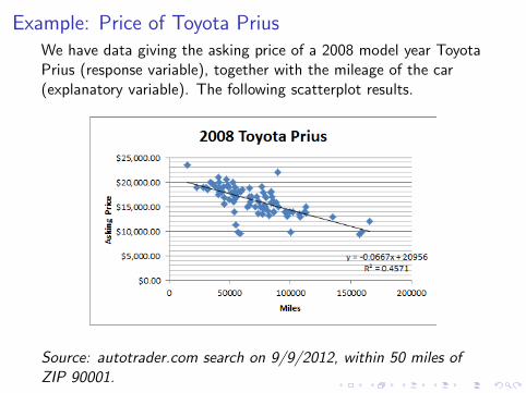
Example: Price of Toyota PriusWe have data giving the asking price of a 2008 model year ToyotaPrius (response variable), together with the mileage of the car(explanatory variable). The following scatterplot results.

Source: autotrader.com search on 9/9/2012, within 50 miles ofZIP 90001.

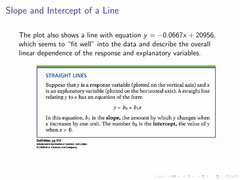
Slope and Intercept of a Line

The plot also shows a line with equation y = −0.0667x + 20956,which seems to “fit well” into the data and describe the overalllinear dependence of the response and explanatory variables.

Example: Price of Toyota Prius

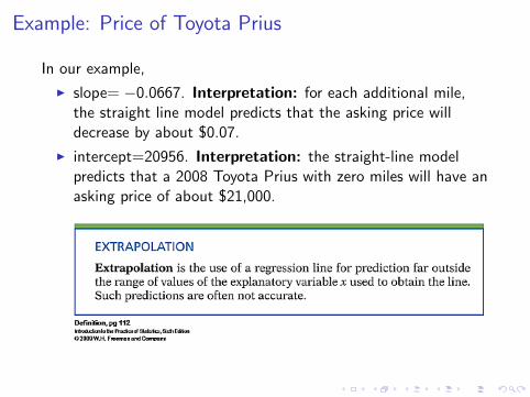
In our example,

I slope= −0.0667. Interpretation: for each additional mile,the straight line model predicts that the asking price willdecrease by about $0.07.

I intercept=20956. Interpretation: the straight-line modelpredicts that a 2008 Toyota Prius with zero miles will have anasking price of about $21,000.

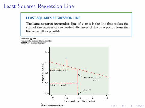
Least-Squares Regression Line

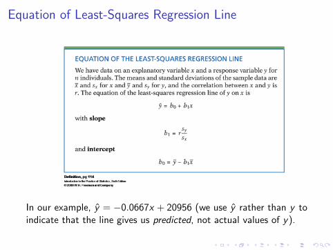
Equation of Least-Squares Regression Line

In our example, y = −0.0667x + 20956 (we use y rather than y toindicate that the line gives us predicted, not actual values of y).

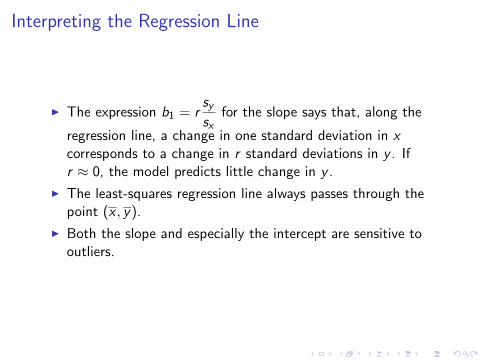
Interpreting the Regression Line

I The expression b1 = rsysx

for the slope says that, along the

regression line, a change in one standard deviation in xcorresponds to a change in r standard deviations in y . Ifr ≈ 0, the model predicts little change in y .

I The least-squares regression line always passes through thepoint (x , y).

I Both the slope and especially the intercept are sensitive tooutliers.

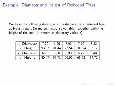
Example: Diameter and Height of Redwood Trees

We have the following data giving the diameter of a redwood treeat breast height (in meters, response variable), together with theheight of the tree (in meters, explanatory variable).

x : Diameter 7.22 6.25 7.92 7.10 7.22

y : Height 93.57 91.44 97.54 103.94 87.17

x : Diameter 6.16 6.00 6.90 5.79 6.40

y : Height 80.47 95.71 99.06 65.53 77.72

Example: Diameter and Height of Redwood Trees

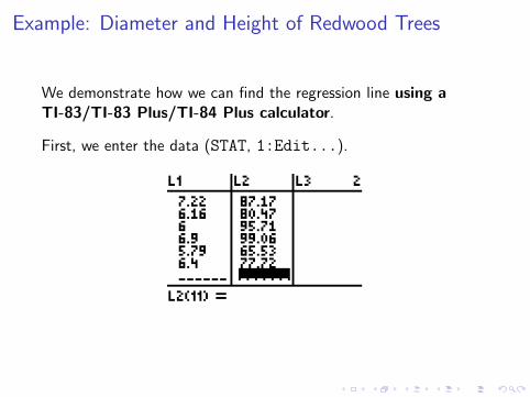
We demonstrate how we can find the regression line using aTI-83/TI-83 Plus/TI-84 Plus calculator.

First, we enter the data (STAT, 1:Edit...).

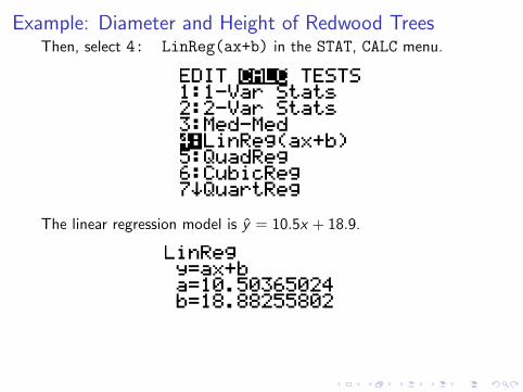
Example: Diameter and Height of Redwood TreesThen, select 4: LinReg(ax+b) in the STAT, CALC menu.

The linear regression model is y = 10.5x + 18.9.

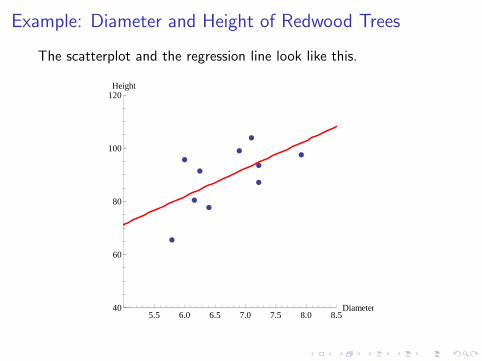
Example: Diameter and Height of Redwood Trees

The scatterplot and the regression line look like this.

5.5 6.0 6.5 7.0 7.5 8.0 8.5Diameter40

60

80

100

120Height

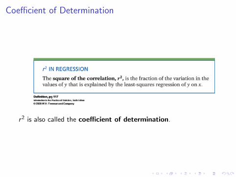
Coefficient of Determination

r2 is also called the coefficient of determination.

Example: Diameter and Height of Redwood Trees

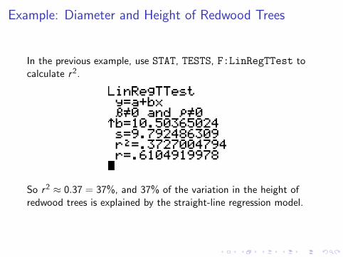
In the previous example, use STAT, TESTS, F:LinRegTTest tocalculate r2.

So r2 ≈ 0.37 = 37%, and 37% of the variation in the height ofredwood trees is explained by the straight-line regression model.

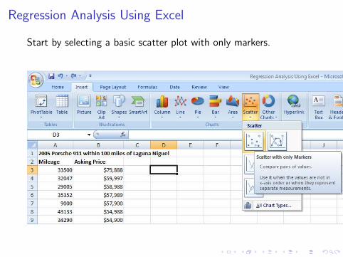
Regression Analysis Using Excel

Start by selecting a basic scatter plot with only markers.

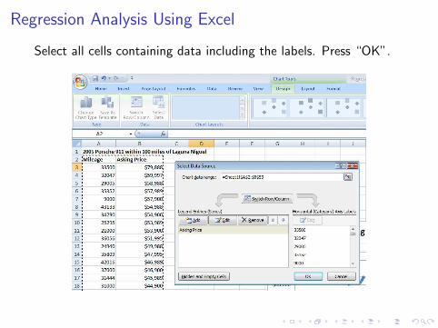
Regression Analysis Using Excel

Select all cells containing data including the labels. Press “OK”.

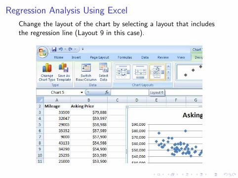
Regression Analysis Using Excel

Change the layout of the chart by selecting a layout that includesthe regression line (Layout 9 in this case).

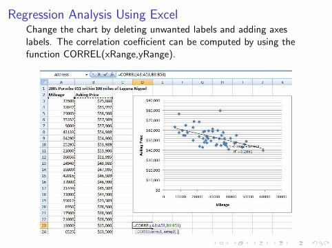
Regression Analysis Using ExcelChange the chart by deleting unwanted labels and adding axeslabels. The correlation coefficient can be computed by using thefunction CORREL(xRange,yRange).