Embed Size (px)
Citation preview

Near-Collinearity and the Orthogonalization ofRegressors: Anscombe’s Quartet New Insights on
Tests for Non-Linearity
Jean-Bernard Chatelain∗and Kirsten Ralf†
March 30, 2009
Abstract
This note presents differents orthogonalizations of regressors facing near-collinearity and constrained parameters regressions.JEL classification: C10, C12Keywords: Collinearity, Student t Statistic.
1. Introduction
Near-collinearity (or near-multicollinearity or collinearity) between explanatory vari-ables is defined for high values of multiple correlations between explanatory variablesin multiple regression. Near collinearity does not invalidate the assumptions of ordi-nary least squares, as long as the collinearity is not perfect: in this case, the estimatorcannot be computed. Near-collinearity may lead to high values of the estimated pa-rameters, high values of the estimated variance of each parameters, and low values ofthe t statistics. Near-collinearity is a problem for the selection of variables.As a consequence, a general to specific specification search usually orthogonalizes
the regressors, in order to select relevant variables. However, there exists differentmethods for the orthogonalization of regressors, leading to different t-statistics anddifferent inference on selected variables. This paper deals with two of these orthogo-nalization methods: the Gram Schmidt Choleski hierarchical orthogonalization, wherethe order of the variables matters in the orthogonalization, and a more ”egalitarian”treatment of regressors: the standard principal component analysis. Note that Halland Fomby [2003] and Buse [1984] mention that the parameter of the favoured regres-sor in the Gram Schmidt orthogonalization method may be biased and inconsistent.
∗Centre d’Economie de la Sorbonne (CES), Paris School of Economics, and CEPREMAP, Uni-versity Paris 1 Pantheon Sorbonne, E-mail: [email protected]
†ESCE, Graduate School of International Trade, Paris, CEPREMAP, E-mail: [email protected]

On the other hand, Hendry and Nielsen [2007] mention that a hierarchy is explainedby substantive reasons, and propose to use it for quadratic models.A particular case of models plagued by near-multicollinearity are multiple poly-
nomial models, such as quadratic models with interaction terms (Hendry, Krolzig,etc.). Multiple polynomial models of order 2, 3 or 4 are a local approximation of moregeneral non-linear models. As such, there have been used as a specification to testfor non-linear model (White [1980], Castle and Hendry [2009]). Castle and Hendry[2008] propose a low dimension collinearity robust test for non linearity. In a ingenu-ous test, Castle and Hendry [2008] orthogonalize the quadratic and interaction termsusing the principal component analysis, which greatly reduces the dimensionality ofthe White test [1980]. A potential extension of their test is to orthogonalized first allthe quadratic and interaction terms with respect to all the linear terms (favored byHendry and Nielsen [2007]) and then go on with these residuals for their tests.We propose here a non-linear test where all the orthogonalizations possible for
all the possible hierarchy or orders of the Gram-Schmidt-Choleski procedure and thePrincipal Component are used: the specification which is chosen is the one with thehighest t-statistic. This note presents differents orthogonalizations of regressors facingnear-collinearity and constrained parameters regressions.To evaluate the procedure, we use a famous data set with four polar cases using
Anscombe’s quartet. We use Anscombe first three small samples of 11 observationswith the same correlation coefficient of the dependent variable and the regressor,and the same correlation coefficient of the regressor and its square (and a high near-multicolllinearity, but not an exact one, which is the case of Anscombe fourth sample).The first sample is related to a true linear model, the second to a true quadratic model,the third to a true linear model with an outlier, and we construct a fourth one of atrue quadratic model with zero or near-zero correlation of the dependant variable withthe regressor and the square of the regressor (described as a near-spurious regression”,in a companion paper (Chatelain and Ralf [2009]). The outcome of the procedure areas follows.- In the first case, a pair of non orthogonalized near-collinear would be eliminated
in a general to specific approach (with a power of the t test very low, because thegain in R2 by adding one regressor with respect to the simple regression is very small)whereas the procedure that we propose would retain only the linear term, which isprefered to the first principal component and to the quadratic term only.- In the second case, a pair of non orthogonalized near-collinear is kept in a general
to specific approach, as well as both orthogonalized regressors in the three method (2gram Schmidt and the complete PC-OLS). A regression with near-collinear variablemay be very precise, because the root mean square error of the residual is very small,so that orthogonalization is not necessary.- In the third case, the method selects the square term only model (a non linear
model). However, this selection procedure fails to notice that the non linear model ischosen only because of an outlier. The true model is a linear one with an outlier. A
2
model with the linear term and a dummy for the outlier outperforms the quadraticmodel by a gain of 32% of variance for the coefficient of determination.- In the fourth case, the method selects both regressors, with a large power of the
t-test (the gain in R square when adding any of the two regressors with respect to thesimple regression is near unity). However, this results presents a substantive paradox.First, each of the regressors explain 0% or 2% of the variance of the dependent vari-able, whereas together they explain 100% of the variance of the dependent variable.Second, the second principal component or the residual of one regressors with respectto the other (both new variables are close to the difference of the two near-collinearregressors), which accounts for 0.6% of the total variance of the two regressors, isable to explain 99.4% of the variance of the dependent variable. This challenges thecommonly held view that the difference of a pair of near-collinear variables is usuallynot precisely estimated (e.g; Verbeek [2000], p.40). The selection of the relevant or-thogonalized variable is the second axis (with lowest variance of the regressors, andhence, a large standard error of its parameters) instead of the first one as in othercases (1, 2 and 3 ) is a particular property of near-spurious regressions. It is then asubstantive issue to state whether the difference of there two variables makes sense insuch a regression. This raises light on a old debate with respect to selecting principalcomponents on the bases of the eigenvalues or on the basis on t-statistics (Jolliffe). Ina SAS book, the insight proposed was that there was outliers leading to specific effects,a mixture of the problem identified in case 2 (with r12 large) and the near-spuriousregression of case 4.Another section investigates the ”ceteris paribus”. For example, Verbeek [2000]
suggests that the ”ceteris paribus” interpretation is not valid in case of near-multicollinearity.This section goes further using the usual interpretation of standardized coefficientswhen they exceed unity. In this case, a ceteris paribus interpretation over-forecastextreme tails of the distribution of the dependent variable. In practice, full effectsimple correlation are reliable to evaluate the effect of near-collinear variables. Thelogical consequences of Verbeek’s points is the following: the ceteris paribus is onlyexactly valid with orthogonalized regressors, or with complete simple regression ef-fects and not with partial correlation effects. The ”ceteris paribus” interpretation ofstandardized coefficients larger than unity is dubious.Finally, the paper discusses in practice how cases 2 and case 4 in various literature:
investment and polynomial adjustment costs, aid and growth literature.The paper proceeds as follows. Section 1 presents the orthogonalization of regres-
sors. Section 2 presents various constrained parameters regressions
2. Near-collinearity: Definition
Let us consider a regression on standardized variables (hence, there is no constant inthe model). Bold letters corresponds to matrices and vectors.
x1 = Xkβ + ε
3
where x1 is the vector of N observations of the explained variable, X.k is the matrixwhere column i corresponds to the N observations of the regressor xi for 2 ≤ i ≤ k+1,bβ is a vector of k parameters to be estimated, and ε is a vector of random disturbancesfollowing a normal distribution of mean zero and of variance σ.Let us denoteRk+1 a block sample correlation matrix between all variables, includ-
ing the explained variable on the first row and column. The matrix Rk correspondsto the correlation matrix of the regressors. One has r2ij ≤ 1 for 1 ≤ i ≤ k + 1 and1 ≤ j ≤ k + 1.
Rk+1 =
"1 r
01
r1 Rk
#with Rk =
1
NX0kXk = [rij]2≤i≤k+1
2≤j≤k+1and with r1 = X
0kx1 = [r1i]2≤i≤k+1
A correlation matrix is positive. Its determinant is such that 0 ≤ det (Rk+1) ≤ 1,for all values of k ≥ 1. Let us denote Rk+1/Rk the Schur complement of the matrixRk+1 defined by:
Rk+1/Rk = 1− r01R
−1k r1 = 1−R21.23...k ≥ 0
Because r1 is a one column matrix, the Schur complement Rk+1/Rk is a scalar.It is equal to one minus the coefficient of determination of the multiple correlationR21.23...k, so that: 0 ≤ Rk+1/Rk ≤ 1. A property of Schur complement is (Puntanenand Styan [2005]):
0 ≤ det (Rk+1) = det (Rk+1/Rk) · det (Rk) =³1−R21.23...k+1
´det (Rk) ≤ det (Rk) ≤ 1
Let us define:(1) Exact collinearity between regressors for det (Rk) = 0.(2) Near-collinearity between regressors when 0 < det (Rk) ≤ δ < 1, with δ is
relatively small, defined by a rule of thumb such as δ = 0.1.(3) An exact multiple regression (exact collinearity between the explained variable
and its regressors) for det (Rk+1) = 0 and det (Rk) 6= 0.Problems related to near-collinearity:(1) large (or small) estimated parameters.(2) large (or small) estimated standard errors.(3) small (or large) t statistics.(4) small (or large) coefficient of determination.(5) Sensitivity of the removal or the addition of observations in the sample: possible
large variation on all estimates, possible change of signs of the parameters, while theparameters remains large in both the positive and the negative case.(6) Poor forecasting properties out of the sample of estimation, while the model
may look good in the sample. This property is also related to some extent with”over-fitting”: too many regressors increases the probability of near-collinearity.(7) In automatic model selection, with near collinearity between relevant and irrel-
evant regressors, it would become difficult to correctly eliminate irrelevant regressors.
4
This can however be avoided through orthogonalization. The order of the orthogonal-ization will matter, and results in different selected models, which could be compared us-ing encompassing and evaluated in the substantive context (Hendry and Nielsen [2007],page 297). For example, it has been observed that automatic selection models suchas stepwise may not select the ”best” variables when there is near-collinearity. Thisinference problems are mentioned as ”pre-test bias”, ”selection bias”, ”post-modelselection bias” (Hendry and Nielsen [2007], page 113).How frequent is near-collinearity?- For time series:(TS1) Dynamic models with lags: r (xt, xt−1) could be large.(TS2) Time series linear function on time (common coefficient = common trend,
or not), non linear function of time (cyclical component, seasonal component): tworegressors are function of a third factor (time).- For times series and cross sections:(TSCS1) Non linear in the variables model: polynomial models (quadratic, cubic,
quartic):
- r³x, xk
´increases when the mean of the observations is far from zero.
- r³x2k+1, x2k
0+1´> r
³x2k+1, x2k
0´, the correlation of two odd (respectively two
even) powers is higher than the correlation of an odd with and even power, when themean of the sample observations is close to zero.- Multiple polynomial: interaction terms. r (x1, x1x2) and r (x2, x1x2) are generally
high correlations.(TSCS2) Endogeneity:- one of the regressors is endogenous and function of the other: x3 = bβ23x2 + ε23.- regressors depends on a common (non measured) third factor, which is not nec-
essarily ”time”. For example, indicators measuring with errors more or less the samephenomenon.Estimated frequency: Near multicollinearity is likely to occur in one multiple re-
gression over five or ten.
3. Complete and Incomplete Principal Component RegressionModel
Let P be the k×k matrix consisting of k×1 orthonormal eigenvectors pij (1 ≤ i ≤ k)of the correlation matrix 1
NX0NkXNk (we do not mention the indices of dimensions for
k × k matrix). The matrix P is orthogonal: P−1= P0. A diagonal k × k matrix ofeigenvalues Λ is such that:
1
NX0NkXNk= PΛP
0 =³P√Λ´ ³√
ΛP0´= P1P
01
5
The sum of the diagonal elements (the trace) of a correlation matrix is equal tok because its diagonal elements are all equal to unity. The trace of a matrix is alsoequal to the sum of its eigenvalues:
trace (Rk) = k = trace³PΛP−1
´= trace (Λ) =
i=kXi=1
λi ⇒1
k
i=kXi=1
λi = 1
Hence, the average value of the eigenvalues of a correlation matrix is equal to unity.Because a correlation matrix is positive, all its eigenvalues are positive. Hence, if thereis one eigenvalue over unity, there exist necessarily another eigenvalue below unity.The N ×k matrix of mutually orthogonal principal components ZNk stands in the
following relation to XNk:
ZNk = XNkP and XNk= ZNkP0
The correlation matrix of mutually orthogonal principal components is:
1
NZ0NkZNk =
1
N(XNkP)
0XNkPXNk = Λk
The variances of each principal component is equal their respective eigenvalue.The principal components related to near zero eigenvalues have very little variance.The principal components (each of the column vectors of the matrix Zk) could bestandardized to have unit standard errors and unit variance by premultiplying by the
inverse of the diagonal matrix of standard deviations, namely Λ− 12
k :
ZSNk = Λ− 12
k XNkP =
Ãz1√λ1, ...,
zk√λk
!with ZS0NkZ
SNk = N · Ik
Substituting this equation in the regression equation for X, the relation betweenthe dependent variable
x1 = XNkβ + ε = ZNkP0β + ε = ZNkβPC + ε
where βPC is the k × 1 vector of population parameters corresponding to theprincipal components Zk. Using properties of orthogonal matrix, the OLS estimatesof the orignial parameters in equation (1) can be formed as:
bβPC = (Z0NkZNk)−1Z0NkY =(P0X0
NkXNkP)−1P0X0
NkYN
= P0 (X0NkXNk)
−1PP0X0
NkYN= P0 (X0
NkXNk)−1X0NkYN= P
0 bβbβPC = P0 bβ ⇔ bβ = PbβPCHence, the estimated residuals bε do not change after orthogonalisation includ-
ing ALL the principal components. The residuals, the root mean square error (the
6

estimated standard error of the residuals), the coefficient of determination R2, thepredictor bx1 are identical, in both the orthogonal and non-orthogonal regression (theyalso exhibit the identical likelihood, see Hendry and Nielsen [2007], p.106). Hence, theorthogonalization of regressors matters only for inference when selecting the relevantvariables (t-test).The estimated variance of the estimated parameter for the ith principal compo-
nent is the root of the ith diagonal entry of the covariance matrix of parameters. Itrepresents an orthogonal decomposition of the variance of the estimates before theorthogonalization:
V³bβPC´ = σ2ε · (Z0NkZNk)
−1= σ2ε · (P0X0
NkXNkP)−1=σ2ε · (NΛ)
−1
Because the variance of the principal components related to near zero eigenvaluesis very small, the parameters of these principal components are likely to be not pre-cisely estimated, except when the estimated standard error bσ2ε is very small (or whendet (Rk+1) is very small).Conversely, for the non orthogonal initial estimates, one has the variance orthog-
onal decomposition (provided by the option PROC REG, Model / COLLIN):
σ2³ bβi´ = σ2ε · (X0
NkXNk)−1= σ2ε · (NPΛP0)
−1= σ2ε
1
N
j=kXj=1
p2ijλj
Bounds:j=kXj=1
p2ij = 1, 0 ≤ p2ij ≤ 1
The properties of orthogonal matrix implies that p2ij are bounded. The parameterswill be more precisely estimated, when one deletes components with the smallest λjwhich greatly increases the standard errors in case of near-collinearity.The incomplete principal component regression (IPC-OLS) estimate of the matrix
βIPC is an estimate that is formed by deleting the effects of certain components inestimating β. This amounts to replacing certain column orthonormal eigvenvectors ofP with zero vectors resulting in a new matrix P∗. In this case, if the first regression isthe true model, the estimates will be biased and the estimated residuals are different.There gain in the reduction of standard errors for the remaining components are notalways granted for two reasons:- In some cases with more than 2 variables, p2ij may be very small as well.
- The omitted variable bias on bβIPC due to the omission of some principal compo-nents may increase the residuals, which may increase the mean square error (MSE)used to estimate σ2ε and determines an omitted variable bias on the estimated stan-dard error of the estimated parameters of the remaining principal components. Then,in some cases (see Anscombe, case 2), the omitted second principal component doesnot reduce the standard error. This last problem is due to the fact that the deletion
7
decisions are made without information regarding the correlation between the depen-dent variable and the regressors. In particular, in the trivariate case, there may be aproblem when r12− r13 turns to be relatively large (for example over 0.03) along withr23 > 0.95.
4. Choleski and QR factorization: Gram Schmidt Orthogonal-ization of the Linear Model
Orthogonalization may be an intermediate computation of matrix numerical analysisinvolved in OLS estimates. Two numerical matrix algorithms are used for solvingthe normal equations of estimates, the unique Choleski factorization or the ”QR”factorization related to Gram Schmidt orthogonalization.Let L1 be a k× k lower (or left) triangular matrix consisting of k× 1 vectors u1,ij
(1 ≤ i ≤ k), with diagonal elements equal to unity u1,ii = 1. The Choleski factorizationof the positive definite symmetric covariance matrix 1
NX0kXk is the product of a lower
triangular matrix L1, of a diagonal matrix Dk with positive diagonal elements, andthe upper triangular matrix L
01 (which is the transpose of the lower triangular matrix
L1):1
NX0NkXNk= L1DL
0
1 =³L1√D´ ³√
DL01
´= LL
0
The matrix L is a k × k lower triangular matrix consisting of k × 1 vectors u1,ij(1 ≤ i ≤ k), where all diagonal elements are strictly positive and equal to u1,ii =
√dk.
If rank (Xk) = k, then L and its transpose are invertible. The diagonal matrixdiffers from the diagonal matrix of eigenvalues, but the trace and the determinantsof both matrices are identical. The transition matrix is lower triangular instead ofbeing orthogonal and including normalized eigenvectors as in the principal componentsorthogonalization. The matrix Dkk is diagonal and easy to invert. Using the rule forthe inverse of a matrix products, we can then compute:µ
1
NX0NkXNk
¶−1=³L01
´−1D−1L−11 =
³L−11
´0D−1L−11
Remark: the inverse of a lower triangular matrix is a lower triangular matrix.However, in general, a lowerr triangular matrix is not necessarily orthogonal (suchthat L0 = L−1).The N×k matrix of the vectors of observations of orthogonal variables ZNk stands
in the following relation to the matrix of the vectors of observations of the (non-orthogonal) variables XNk (matrix numerical analysis textbooks uses the notationQR factorization instead of our notation: Z
√DL
01):
ZSNk = XNk
³L0´−1
= XNk
³√DL
01
´−1⇔ XNk= Z
SNkL
0= ZSNk
√DL
01
Let us check that the matrix ZSNk is orthogonal (its column vectors are mutuallyorthogonal), which is the cae if the Gram matrix of the column vectors is diagonal
8
(Gram Schmidt orthogonalization procedure). If the Gram matrix of column vectorsis equal to the unit matrix, the variance of each column vector is equal to unity: thecolumn vectors are standardized in the sample, due to the termD−1/2 (Gram Schmidtorthonormalization procedure):
ZS0NkZSNk =
µXNk
³L0k
´−1¶0XNk
³L0k
´−1=µ³L0k
´−1¶0X0NkXNk
³L0k
´−1= L−1k LkkL
0kk
³L0k
´−1= Ik
Substituting this equation in the regression equation forXNk, the relation betweenthe dependent variable and the regressors are:
x1 = XNkβ + ε = ZNk³L0´−1
β + ε = ZNkβGS + ε
where βGS is the k × 1 vector of population parameters corresponding to theGram Schmidt orthogonalization ZNk. Using properties of orthogonal matrix, theOLS estimates of the original parameters in equation (1) can be formed as:
bβGS = (Z0NkZNk)−1Z0NkY = LX0Y
=³L0´−1
(X0kXk)
−1L−1LX0Y =
³L0´−1
(X0X)−1X0Y =
³L0´−1 bβ
bβ = L0 bβGS and bβGS = ³
L0´−1 bβ
Hence, the estimated residuals bε do not change after orthogonalisation includingALL the orthogonalized explanatory variables. The predictions bx1 are not changed,as well as all statistics using estimated residuals such as R2, RMSE, and Durbin-Watson statistics for time series. It is only the parameter estimates and the estimatedstandard errors which benefit from orthogonalization.Note that:
bβGS = (Z0NkZNk)−1Z0NkY = D−1Z0NkY
Solving the normal equations for the computation of OLS estimate knowing theCholeski factorization 1
NX0kXk = LL
0 amounts to solve two triangular systems (withinverse matrix easy to compute):
(X0NkXNk) bβ = LL
0 bβ = X0NkY
solve LbβGS = X0NkY ⇒ bβGS = L−1X0
NkY = Z0Y
then solve L0 bβ = bβGS ⇒ bβ = (L0)−1 bβGSHence, the parameters of orthogonal are an intermediate numerical computation
of bβ in most softwares. Solving the normal equations for the computation of OLSestimate knowing the ”QR” factorization XNk= ZNkL
0 amounts to solve only the lasttriangular systems of the Choleski method (with inverse matrix easy to compute):
9

(X0NkXNk) bβ = X0
NkY⇒³(ZL0)
0ZL0
´ bβ = (ZL0)0Y⇒(LZ0ZL0) bβ = LZ0Y⇒ solve: L0 bβ = bβGS = Z0Y
The estimated variance of the estimated parameter for the ith principal compo-nent is the root of the ith diagonal entry of the covariance matrix of parameters. Itrepresents an orthogonal decomposition of the variance of the estimates before theorthogonalization:
V³bβGS´ = σ2ε ·
³ZS0k Z
Sk
´−1= σ2ε · (NI)
−1
On the other hand, for the non orthogonal initial estimates, one has the varianceorthogonal decomposition:
σ2³ bβi´ = σ2ε · (X0
kXk)−1= σ2ε · (NLL0)
−1= σ2ε
1
N
j=kXj=1
u21,ijdj
This is a ”hierarchical” orthogonalization, in the sense that the full effect (the simplecorrelation coefficient) is taken into account for the first variable and only the partialeffect for the second variable (the in sample residual of the auxiliary regression). Bycontrast, the principal component is an egalitarian divide of the information providedby each variables.This is the method proposed by Hendry and Nielsen (Chapter 7, p.107): ”Orthog-
onalization requires a hierarchy of the regressors to determine which regressors shouldbe orthogonalized with respect to which. In most applications, econometric models willhave a richer structure than theory models. Such a framework could suggest a hierar-chy”. ”The wage schooling relation gives an example, with the levels and squares ofschooling being highly correlated. Given the context, it seems more natural to orthogo-nalize the square with respect to the linear term than vice versa” (Hendry and Nielsen(p.137)). A linear model is simpler than a non linear model and may be given priority.By contrast, Buse [1994] mentions that this hierarchical orthogonal model bias theestimate bβ12 of the first variable (by the − bβ”13r23) and bias its estimated standarderror (a biased and inconsistent estimator), because there is an omitted variable ofthe component r23x2 in the regression. However, the full effect of the first variable iscorrect for ceteris paribus interpretation of the parameter bβ1.2.Incomplete regressions with orthogonal regressors:(1) Principal component regression: one decides to omit the principal component
axis with the lowest eigenvalue (the lowest share of variance) or with the lowest nonsignificant t-statistic. This is known as the ”Incomplete Principal Component Regres-sion”.(2) With the hierarchic orthogonal regression, one decides to omit one of the vari-
ables, i.e.: the residual of a regression between two near-collinear variables.(3) One may omit directly one of the two variables.
10

5. The Trivariate Regression
5.1. Properties of the trivariate regression
Let us now consider the trivariate case (k = 2) for standardized variables. With near-collinearity, precise regressions (relatively small standard errors and large t statistics)are easily found. In these cases, a metric able to evaluate whether coefficients areoversized is needed for authors, referes and journal editors. First, let us considerstandardized parameters:
x1 − x1σ1
= bβ12x2 − x2σ2
+ bβ13x3 − x3σ3
+ ε1.23
The interpretation of a standardized parameter is as follows: a deviation from themean of the regressors x2 by one standard error σ2 of this regressor (that is:
x2−x2σ2
= 1)imply a prediction bx1 which deviates from the mean of the explained variable x1 bybβS12 times the standard error of the explained variable σ1. In the case of the simpleregression, the standardized parameter is exactly equal to the correlation coefficientr12, which is such that |r12| ≤ 1. In multiple regression with near collinearity, thestandardized parameter can easily exceed unity.The determinant of correlation matrices, the coefficient of determination, the stan-
dardized coefficients, their standard errors, their t-statistics and their partial correla-tion coefficients are given by:
0 ≤ det (R3) = 1− r212 − r213 − r223 + 2r12r13r23 ≤ det (R2) = 1− r223 ≤ 1
R21.23 = 1− det (R3)
det (R2)=r212 + r
213 − 2r12r13r231− r223
= 1−³1− r212
´ ³1− r213.2
´Ã bβ12bβ13
!=
1
1− r223
"1 −r23−r23 1
#Ãr12r13
!=
1
1− r223
Ãr12 − r13r23r13 − r12r23
!
bσε =
√MSE√N − 2
=
q1−R21.23√N − 2
=1√N − 2
vuutdet (R3)
det (R2)Ã bσbβ1bσbβ2!= RMSE
1
det (R2)diag
"1 −r23−r23 1
#=
qdet (R3)√N − 2
1
1− r223
Ã11
!Ãtbβ1tbβ2
!=
√N − 2qdet (R3)
Ãr12 − r13r23r13 − r12r23
!
−1 < r12.3 =r12 − r13r23q
(1− r213) (1− r223)=
t12qt212 +N − 2
=
q1− r223q1− r213
bβ12 < 1The relation between the partial correlation coefficient r12.3 (once the influence of
the second explanatory variable x3 is removed) and the t12 statistics for parameter bβ12is given in Greeene [2000], p.234-235.
11

In the trivariate case, the three collinearity indicators: the determinant det (R2),the variance inflation factor (V IF ) and the condition index CI depend only on thecorrelation coefficients between r23:
λmax = 1 + r23 and λmax = 1− r23det (R2) = λmaxλmin = 1− r223V IF =
1
1− r223=
1
det (R2)=
1
λmaxλmin
CI =
sλmaxλmin
=
s1 + r231− r23
where λmax = 1+ r23 and λmin = 1− r23 are the two eigenvalues of the correlationmatrix of the regressors R2 (see next section on the principal components orthogo-nalization of regressors). We assume from now on r23 ≥ 0, the alternative leading tosymmetric results easy to find . Hence, near-collinearity can be defined by a uniquerule of thumb such as r23 ≥ 0.95 so that det (R2) < 0.1 or V IF > 10 or CI > 6.24.
5.2. The Standard Principal Components Orthogonalizations of Regressors
The principal component analysis leads to the following orthogonalization of regres-sors:
R2 =
Ã1 r23r23 1
!= P2Λ2P
02 =
à 1√2
1√2
− 1√2
1√2
!Ã1− r23 00 1 + r23
!Ã 1√2
1√2
− 1√2
1√2
!T(5.1)
:With characteristic polynomial of R2: X2 − 2X + 1− r223. The matrix of normalized
eigenvectors is an orthogonal matrix, such that its inverse is equal to its transposeP−12 = P
02. It corresponds here to a rotation of −45 degrees, with the following
normalized eigenvectors and their respective eigenvalues (either both eigenvalues areequal to unity, or one eigenvalue is between 1 and 2 and the other one is between zeroand one):Table 1: Eigenvalues, percentage of variance for each principal components and
normed eigenvectors of the correlation matrix R2:λmin + λmax = k = 2 λmin = 1− r23 (PC2) λmax = 1 + r23 (PC1)over/below unity 0 ≤ λmin = 2− λmax = 1− r23 ≤ 1 1 ≤ λmax = 1 + r23 ≤ 2 (if r23 ≥ 0)% variance λmin
λmin+λmax= 1−r23
2λmax
λmin+λmax= 1+r23
2
x21√2= .70711 = cos
³π4
´1√2= .70711 = cos
³π4
´x3 − 1√
2= −.70711 = − sin
³π4
´− 1√
2= .70711 = sin
³π4
´Let us now turn to the matrix R3 taking into account the orthogonalization ac-
cording to the principal component analysis of the regressors:
12
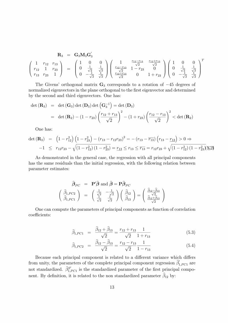
R3 = G3M3G03⎛⎜⎝ 1 r12 r13
r12 1 r23r13 r23 1
⎞⎟⎠ =
⎛⎜⎜⎝1 0 00 1√
21√2
0 − 1√2
1√2
⎞⎟⎟⎠⎛⎜⎜⎝
1 r12−r13√2
r12+r13√2
r12−r13√2
1− r23 0r12+r13√
20 1 + r23
⎞⎟⎟⎠⎛⎜⎜⎝1 0 00 1√
21√2
0 − 1√2
1√2
⎞⎟⎟⎠T
The Givens’ orthogonal matrix G3 corresponds to a rotation of −45 degrees ofnormalized eigenvectors in the plane orthogonal to the first eigenvector and determinedby the second and third eigenvectors. One has:
det (R3) = det (G3) det (D3) det³G−13
´= det (D3)
= det (R2)− (1− r23)Ãr12 + r13√
2
!2− (1 + r23)
Ãr12 − r13√
2
!2< det (R2)
One has:
det (R3) =³1− r212
´ ³1− r223
´− (r13 − r12r23)2 = − (r13 − r13)
³r13 − r13
´> 0⇒
−1 ≤ r12r23 −q(1− r212) (1− r223) = r13 ≤ r13 ≤ r13 = r12r23 +
q(1− r212) (1− r223) ≤ 1(5.2)
As demonstrated in the general case, the regression with all principal componentshas the same residuals than the initial regression, with the following relation betweenparameter estimates:
bβPC = P0 bβ and bβ = PbβPCÃ bβ1,PC2bβ1,PC1!=
à 1√2− 1√
21√2
1√2
!Ã bβ12bβ13!=
⎛⎝ bβ12−bβ13√2bβ12+bβ13√2
⎞⎠One can compute the parameters of principal components as function of correlation
coefficients:
bβ1,PC1 =bβ12 + bβ13√
2=r12 + r13√
2
1
1 + r13(5.3)
bβ1,PC2 =bβ12 − bβ13√
2=r12 − r13√
2
1
1− r13(5.4)
Because each principal component is related to a different variance which differsfrom unity, the parameters of the complete principal component regression bβ0
1,PC1 are
not standardized. bβS01,PC1 is the standardized parameter of the first principal compo-nent. By definition, it is related to the non standardized parameter bβ12 by:
13
bβPC1 = bβSPC1 σx1σx2+x3√
2
= bβS1,PC1 1√1 + r23
⇒ bβSPC1 = r12 + r13√2
1√1 + r23
bβPC2 = bβSPC2 σx1σx2−x3√
2
= bβSPC2 1√1− r23
⇒ bβSPC2 = r12 − r13√2
1√1− r23
The estimated variance of the estimated parameter for the ith principal componentis given by:
V³bβPC´ = σ2ε · (Z0kZk)
−1= σ2ε · (P0X0
kXkP)−1=σ2ε · (NΛk)
−1
VµbβSPC¶ = σ2ε · (NIk)
−1
The Student’s t statistics:
t³ bβS1,PC1´ =
√NbβS1,PC1σ2ε
=
√N − 2qdet (R3)
q1− r223√1 + r23
r12 + r13√2
t³ bβS1,PC2´ =
√NbβS1,PC1σ2ε
=
√N − 2qdet (R3)
q1− r223√1− r23
r12 − r13√2
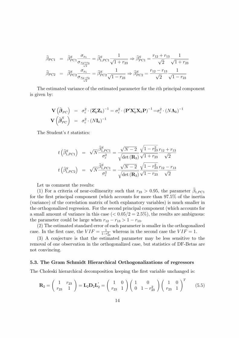
Let us comment the results:(1) For a criteria of near-collinearity such that r23 > 0.95, the parameter bβ1,PC1
for the first principal component (which accounts for more than 97.5% of the inertia(variance) of the correlation matrix of both explanatory variables) is much smaller inthe orthogonalized regression. For the second principal component (which accounts fora small amount of variance in this case (< 0.05/2 = 2.5%), the results are ambiguous:the parameter could be large when r12 − r13 > 1− r13.(2) The estimated standard error of each parameter is smaller in the orthogonalized
case. In the first case, the V IF = 11−r223
whereas in the second case the V IF = 1.
(3) A conjecture is that the estimated parameter may be less sensitive to theremoval of one observation in the orthogonalized case, but statistics of DF-Betas arenot convincing.
5.3. The Gram Schmidt Hierarchical Orthogonalizations of regressors
The Choleski hierarchical decomposition keeping the first variable unchanged is:
R2 =
Ã1 r23r23 1
!= L2D2L
02 =
Ã1 0r23 1
!Ã1 00 1− r223
!Ã1 0r23 1
!T(5.5)
14

The matrix R3 taking into account the Gram Schmidt orthogonalization of regres-sors can be written as:
R3 = H3N3H03⎛⎜⎝ 1 r12 r13
r12 1 r23r13 r23 1
⎞⎟⎠ =
⎛⎜⎝ 1 0 00 1 00 r23 1
⎞⎟⎠⎛⎜⎝ 1 r12 r13 − r12r23
r12 1 0r13 − r12r23 0 1− r223
⎞⎟⎠⎛⎜⎝ 1 0 00 1 00 r23 1
⎞⎟⎠T
The hierarchical orthogonalization of regressors computes orthogonal vectors oneafter the other. In the trivariate case with standardized variables, one computes thein-sample orthogonal vector using the residuals of OLS auxiliary regression betweenregressors:
x3 = r23x2 + ε32 ⇒ cov (x3 − r23x2, x2) = 0
One has the non standardized parameters bβGS:bβGS = (L02)
−1 bβà bβGS1bβGS2!=
Ã1 −r230 1
!Ã bβ12bβ13!=
à bβ12 − bβ13r23bβ13!=
Ãr12
r13−r12r231−r223
!(5.6)
with the standardized parameter:
bβSGS2 = r13 − r12r231− r223
1q1− r223
The Student’s t statistics:
t³ bβS1,PC1´ =
√NbβSGS1σ2ε
=
√N − 2qdet (R3)
q1− r223r12
t³ bβS1,PC2´ =
√NbβSGS1σ2ε
=
√N − 2qdet (R3)
q1− r223q1− r223
r13 − r12r231− r223
If the estimated parameter of ε32 is small and is not significantly different fromzero, then one removes this variable. The regression is then a constrained regressionassuming that the parameter of x2 is equal to zero.
15

5.4. A Comparison of Critical Regions for t statistics with or without or-thogonalization of regressors.
In the four trivariate regressions, the RMSE is identical:
bσε =√MSE√N − 2
=
q1−R21.23√N − 2
=1√N − 2
vuutdet (R3)
det (R2)
But, the standardized parameters and the t-statistics are different. The VIF differsfrom unity when there is no orthogonalization (table 3):
t
√MSE√N − k
= bβS/√V IFTable 3: Standardized parameteres and t statistics.bβS √
V IF√MSE√N−k t
√MSE√N−k R2
A: x r12 1√1−r212√N−1 r12 r212
B: x2 r13 1√1−r213√N−1 r13 r213
C: x+x2
√2
1√1+r23
r12+r13√2
1√1+r23
1√1−R21.2√N−1
r12+r13√2
1√1+r23
(r12+r13)2
21
1+r23
D:x−x2
√2
1√1−r23
r12−r13√2
1√1−r23 1
√1−R21.2√N−1
r12−r13√2
1√1−r23
(r12−r13)22
11−r23
E: x2−r23x√1−r223
r13−r12r231−r223
1√1−r223
1
√1−R21.2√N−1
r13−r12r231−r223
1√1−r223
³r13−r12r231−r223
´21
1−r223
F: x−r23x2√
1−r223r12−r13r231−r223
1√1−r223
1
√1−R21.2√N−1
r12−r13r231−r223
1√1−r223
³r13−r12r231−r223
´21
1−r223
G1: x r12−r13r231−r223
1√1−r223
√1−R21.23√N−2
r12−r13r231−r223
1√1−r223
R21.23
G2: x2 r13−r12r231−r223
1√1−r223
- r13−r12r231−r223
1√1−r223
-
H1:x+x2
√2
1√1+r23
r12+r13√2
1√1+r23
1√1−R21.23√N−2
r12+r13√2
1√1+r23
R21.23H2:x−x
2√2
1√1−r23
r12−r13√2
1√1−r23 1 - r12−r13√
21√1−r23 -
I1: x r12 1√1−R21.23√N−2 r12 R21.23
I2: x2−r23x√1−r223
r13−r12r231−r223
1√1−r223
1 - r13−r12r231−r223
1√1−r223
-
J1: x2 r13 1√1−R21.23√N−2 r13 R21.23
J2: x−r23x2√1−r223
r12−r13r231−r223
1√1−r223
1 - r12−r13r231−r223
1√1−r223
-
The discussion is with respect to:A) The Gram Schmidt (with a hierarchy such as x is the first variable) leads to
reject the null hypothesis more frequently than the non orthogonalized whenN > 100:
t (G) = t (J) =
¯¯r12 − r13r231− r223
1q1− r223
¯¯ < 1.96
√MSE√N − k
< t (I) = |r12|
16

⇒ r12 − r13r23 < r12 ·³1− r223
´ 32 when r12 > 0
⇒ 1.96
√MSE√N − k
< r12 <
⎛⎝ r23
1− (1− r223)32
⎞⎠ · r13 when r23 6= 0 andr23
1− (1− r223)32
≥ 1 and limr23→1
r23
1− (1− r223)32
= 1
B) The complete PC-OLS leads to reject the first principal component null hy-pothesis more frequently than the non orthogonalized when:
t (G) = t (J) =r12 − r13r231− r223
1q1− r223
< 1.96
√MSE√N − k
< t (H) =r12 + r13√
2
1√1 + r23
⇒ r12 − r13r23 <r12 + r13√
2· (1− r
223)
32
√1 + r23
⇒ r12 < r13 ·⎛⎝ (1− r223)
32
√2√1 + r23
+ r23
⎞⎠⎛⎜⎜⎜⎝ 1
1− (1−r223)32
√2√1+r23
⎞⎟⎟⎟⎠check sign.C) The complete PC-OLS leads to reject the first principal component null hy-
pothesis more frequently than the non orthogonalized when:
t (G) = t (J) =r12 − r13r231− r223
1q1− r223
< 1.96
√MSE√N − k
< t (H) =r12 − r13√
2
1√1− r23
⇒ r12 − r13r23 <r12 − r13√
2· (1− r
223)
32
√1− r23
⇒ r12 < r13 ·⎛⎝− (1− r223)
32
√2√1− r23
+ r23
⎞⎠⎛⎜⎜⎜⎝ 1
1− (1−r223)32
√2√1−r23
⎞⎟⎟⎟⎠Then, orthogonalized regressors are able to select significant variables which are
not significantly different from zero when there is near-collinearity.
6. Example: Anscombe’s Quartet
Anscombe four samples leads to the following correlation coefficients for x1 and theregressors x2 and the square value of x
22:
17

Table 3: Anscombe data set correlation matrixr12 (x1, x2) r13 (x1, x
22) r23 (x2, x
22) det (R2) det (R3) R21.23 R21.2 = r
212
1 0.81642 0.78466 0.98818 0.0235 0.00734 0.687 0.6662 0.81624 0.71801 0.98818 0.0235 (”− 3”)× 10−6 1 0.6663 0.81629 0.82742 0.98818 0.0235 0.00741 0.685 0.6664 0.81652 0.81652 1 0 0 − 0.666In all cases, Anscombe constructed the data sets such that their sample correlation
coefficients are nearly identical r12 (x1, x2) = 0.816. Hence, the four simple regressionhave the same slope.In the fourth case, the correlation r23 (x2, x
22) between x2 and x
22 is equal to one,
because x2 has only two distinct numerical values (one corresponds to 10 observationsand the other one to 1 observations). The square of a binary variable remains a binaryvariable. Hence, there is exact collinearity between the two regressors. Hence, one hasr12 = r13. As well, the trivariate regression cannot be computed in this case, becausedet (R2) = 0.The observations of x2 are identical between the cases one, two and three. Hence,
the correlation coefficients r23 (x2, x22) are identical and equal to 0.98818 > 0.95. There
is near-multicollinearity.In cases 1 and 3, the gain in coefficient of determination R21.23 − R21.2 ≈ 0.02 is
small when adding the third variable (the quadratic term).The principal components of the matrix of the regressors are:Case r23 (x2, x
22) det (R2) λmax = 1 + r23 %V ar λmin = 1− r23 %V ar
1, 2, 3 0.98818 0.0235 1.98818 99, 4% 0.01182 0.6%4 1 0 2 100% 0 0%
The percentage of variance accounted for by each principal component are: 99.4%and 0.06%. However, this does not necessarily mean that the second component doesnot matter in a regression with x1, as shown in case 2.The variance of the OLS regression coefficients can be shown to be equal to the
residual variance (RMSE) multiplied by the SUM of the variance decomposition pro-portions (VDP) of all eigenvalues. The most common threshold for a high VDP is ofVDP>0.50 associated with a high condition index:
CI =
sλmaxλmin
=
s1 + r231− r23
=
s1 + 0.98818
1− 0.98818 = 12.969 > 10
The variance decomposition is:
1
1− r223=
p211λ1+p212λ2=
0.5
1 + r23+
0.5
1− r23>>
p211λ1
1
1− 0.988182 = 0.51
1 + 0.98818+ 0.5
1
1− 0.9881842.553 = 0.5 · 0.50297 + 0.5 · 84.602 = 0.25149 + 42.301 = 0.6% + 99.4%
= V DP (λ1) + V DP (λ2)
18
Let us investigate the variance of the parameters of the incomplete principal com-ponents regression. Decomposing the variance of the non orthogonalized standarderror as follows shows that omitting the second principal component axis decreasessharply the standard error of the remaining first principal component. Here, it elimi-nates 99.4% of the variance decomposition proportion (cf. proportion of variance of theother principal component) related to the smallest eigenvalue λ2 = 1− r23 = 0.01182.
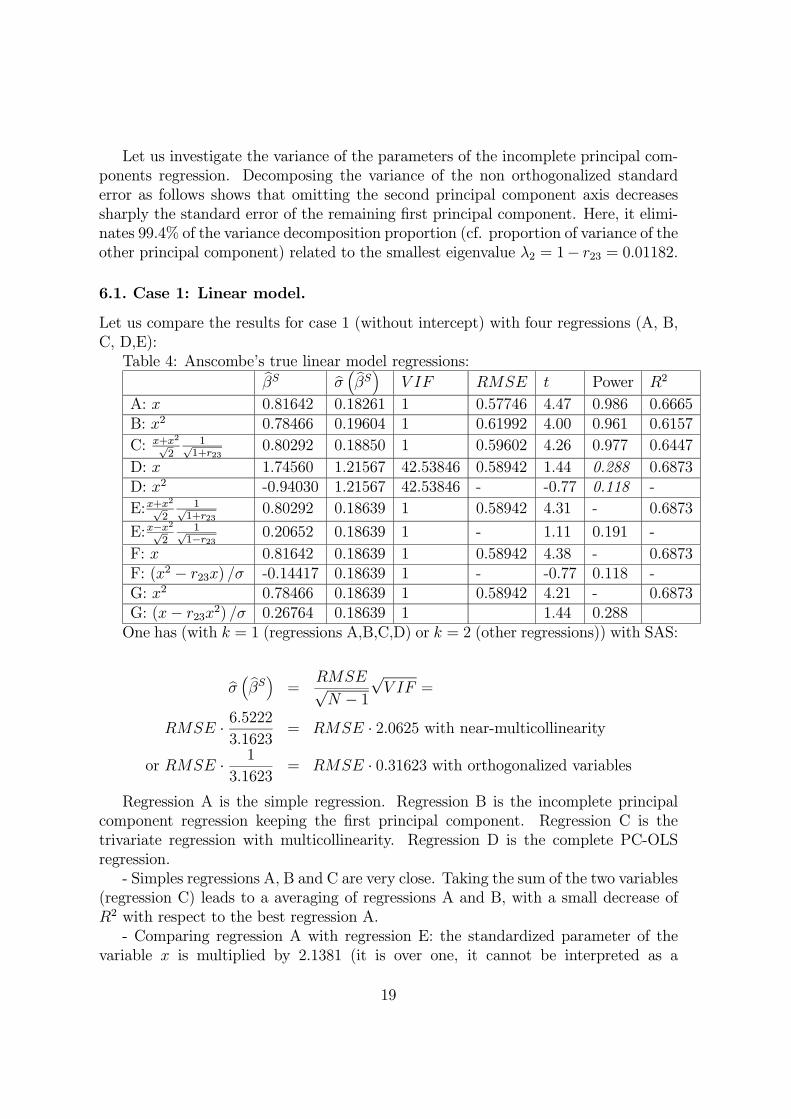
6.1. Case 1: Linear model.
Let us compare the results for case 1 (without intercept) with four regressions (A, B,C, D,E):Table 4: Anscombe’s true linear model regressions:bβS bσ ³ bβS´ V IF RMSE t Power R2
A: x 0.81642 0.18261 1 0.57746 4.47 0.986 0.6665B: x2 0.78466 0.19604 1 0.61992 4.00 0.961 0.6157
C: x+x2
√2
1√1+r23
0.80292 0.18850 1 0.59602 4.26 0.977 0.6447
D: x 1.74560 1.21567 42.53846 0.58942 1.44 0.288 0.6873D: x2 -0.94030 1.21567 42.53846 - -0.77 0.118 -
E:x+x2
√2
1√1+r23
0.80292 0.18639 1 0.58942 4.31 - 0.6873
E:x−x2
√2
1√1−r23 0.20652 0.18639 1 - 1.11 0.191 -
F: x 0.81642 0.18639 1 0.58942 4.38 - 0.6873F: (x2 − r23x) /σ -0.14417 0.18639 1 - -0.77 0.118 -G: x2 0.78466 0.18639 1 0.58942 4.21 - 0.6873G: (x− r23x2) /σ 0.26764 0.18639 1 1.44 0.288One has (with k = 1 (regressions A,B,C,D) or k = 2 (other regressions)) with SAS:
bσ ³ bβS´ =RMSE√N − 1
√V IF =
RMSE · 6.52223.1623
= RMSE · 2.0625 with near-multicollinearity
or RMSE · 1
3.1623= RMSE · 0.31623 with orthogonalized variables
Regression A is the simple regression. Regression B is the incomplete principalcomponent regression keeping the first principal component. Regression C is thetrivariate regression with multicollinearity. Regression D is the complete PC-OLSregression.- Simples regressions A, B and C are very close. Taking the sum of the two variables
(regression C) leads to a averaging of regressions A and B, with a small decrease ofR2 with respect to the best regression A.- Comparing regression A with regression E: the standardized parameter of the
variable x is multiplied by 2.1381 (it is over one, it cannot be interpreted as a
19

”ceteris paribus” effect) but its standard error is multiplied by 6.6572 =√V IF ·
RMSE(C)/RMSE(A): it is no longer significant. As the RMSE is similar in modelA and model C, the increase of the estimated standard error is due to the varianceinflation factor (42.5 times the variance of a model where variables are orthogonal, itmultiplies the standard error by
√V IF = 6.5222 ). For the trivariate regression, the
estimated standard error of standardized parametersare the same for both parameters (this is indeed not the case for non-standardized
parameters, where the standard error is multiplied by σ (x1) /σ (xi)). The parameterof x2 is negative (may be an unexpected sign), large and close of the difference forthe parameter of x in regression Its standard error is relatively large, and it is notsignificantly different from zero. The gain of R2 is very small.- Comparing model A with model D: the standardized coefficient is close to the sim-
ple regression, with a similar t statistic (t statistics are identical for standardized andnon standardized parameters). The second principal component is not significantlydifferent from zero.- Comparing model E with model A and model D: the standardized coefficient is
identical to the simple regression. However, its estimated standard error is identical tothe one of the PC-OLS. Then its t-statistics is very small. The standardized orthogonalresidual of the square of x2 with respect to x has a negative and relatively smallstandardized coefficient. It is not significantly different from zero.A general to specific specification search based on t-test without orthogonalization
starting by regression C would lead to reject both explanatory variables for the nextstep. By contrast, an orthogonalized regression (D or E) would lead to keep the firstprincipal component and to eliminate the second principal component.Note that the reverse error could be true (cf. Roodman [2008] example with
aid/GDP and aid/GPD*tropics): the t-statistics could lead to keep both explanatoryvariables, whereas in an orthogonalized regression, only one of them or none of themis accepted.POWER: The problem of near-multicollinearity with respect to the power of t
tests is the following one:- In regression D: both t-test have low power, because the R2(full model)−R2(restricted
model) is small for both variables.- By contrast, in hierarchical orthogonalized regressions: for the favoured vari-
able, its t-test have high power because the R2(full model)−R2(restricted model) islarge. For the residual variable, it has the same power than in the non-orthogonalizedregression D.- With the complete PC-OLS regression, the second principal component has a
power of its t-test which is between the power of each of the residual variable in thehierarchical model.
20

6.2. Case 2: Non Linear Quadratic model
Table 5: Anscombe’s true quadratic model regressions (A, B, C, D):bβS bσ ³ bβS´ V IF RMSE t Power R2
A: x 0.81624 0.18269 1 0.57772 4.47 0.986 0.6662B: x2 0.71801 0.22011 1 0.69604 3.26 0.860 0.5155
C: x+x2
√2
1√1+r23
0.76940 0.20200 1 0.63877 3.81 0.943 0.5920
D: x 4.53964 0.00160 42.53846 0.00077613 2835.93 >.999 1D: x2 -3.76796 0.00160 42.53846 - -2353.90 >.999 -
E:x+x2
√2
1√1+r23
0.76940 0.00024543 1 0.00077613 3134.85 - 1
E:x−x2
√2
1√1−r23 0.63877 0.00024543 1 - 2602.60 >.999 -
F: x 0.81624 0.00024543 1 0.00077613 3325.68 - 1
F: x2−r23x√1−r223
-0.57772 0.00024543 1 - -2353.9 >.999 -
G: x2 0.71801 0.00024543 1 0.00077613 2925.46 - 1
G: x−r23x2√
1−r2230.69603 0.00024543 1 - 2835.93 >.999 -
- Simples regressions A, B and C are very close. Taking the sum of the two variables(regression C) leads to a averaging of regressions A and B, with a small decrease ofR2 with respect to the best regression A.- Comparing regression A with regression C: the standardized parameter of the
variable x is multiplied by 5.5616 (it is over one, it cannot be interpreted as a ”ceterisparibus” effect). Its standard error is multiplied by 6.6572 =
√V IF ·RMSE(C)/RMSE(A):
it is highly significantly different from zero. As the RMSE is close to zero in modelC, the estimated standard error of this standardized parameter is close to zero despitethe high variance inflation factor (42.5 times the variance of a model where variablesare orthogonal, it multiplies the standard error by
√V IF = 6.5222 ). The parame-
ter of x2 is negative, large and close of the difference for the parameter of x in thesimple regression. Its standard error is identical to the one of the other standardizedparameter. It is highly significantly different from zero. The gain in coefficient ofdetermination R21.23 − R21.2 ≈ 0.33 is large when adding the variable x22 in the model,whereas it does not matter in the cases 1 and 3. In case 2, the model corresponds toa nearly exact regression det (R3) ≈ 0, with negligible residuals,negligible root meansquare error and a coefficient of determination equal to unity.- Comparing model A with model D: the standardized coefficient is close to the
simple regression, with a similar t statistic (t statistics are identical for standardizedand non standardized parameters). The second principal component has a relativelyhigh standardized parameter and it is significantly different from zero.- Comparing model E with model A and model D: the standardized coefficient is
identical to the simple regression. However, its estimated standard error is identicalto the one of the PC-OLS and very small. Then its t-statistics is very large. Thestandardized orthogonal residual of the square of x2 with respect to x has a negative
21
and relatively small standardized coefficient. It is not significantly different from zero.A general to specific specification search based on t-test without orthogonalization
starting by regression C would lead to rightly accept both explanatory variables, aswell as a complete PC-OLS regression.Note that including the second principal component is easier to obtain than in-
cluding the Gram Schmidt residual variable, because the information content betweeneach variable is less asymmetric.
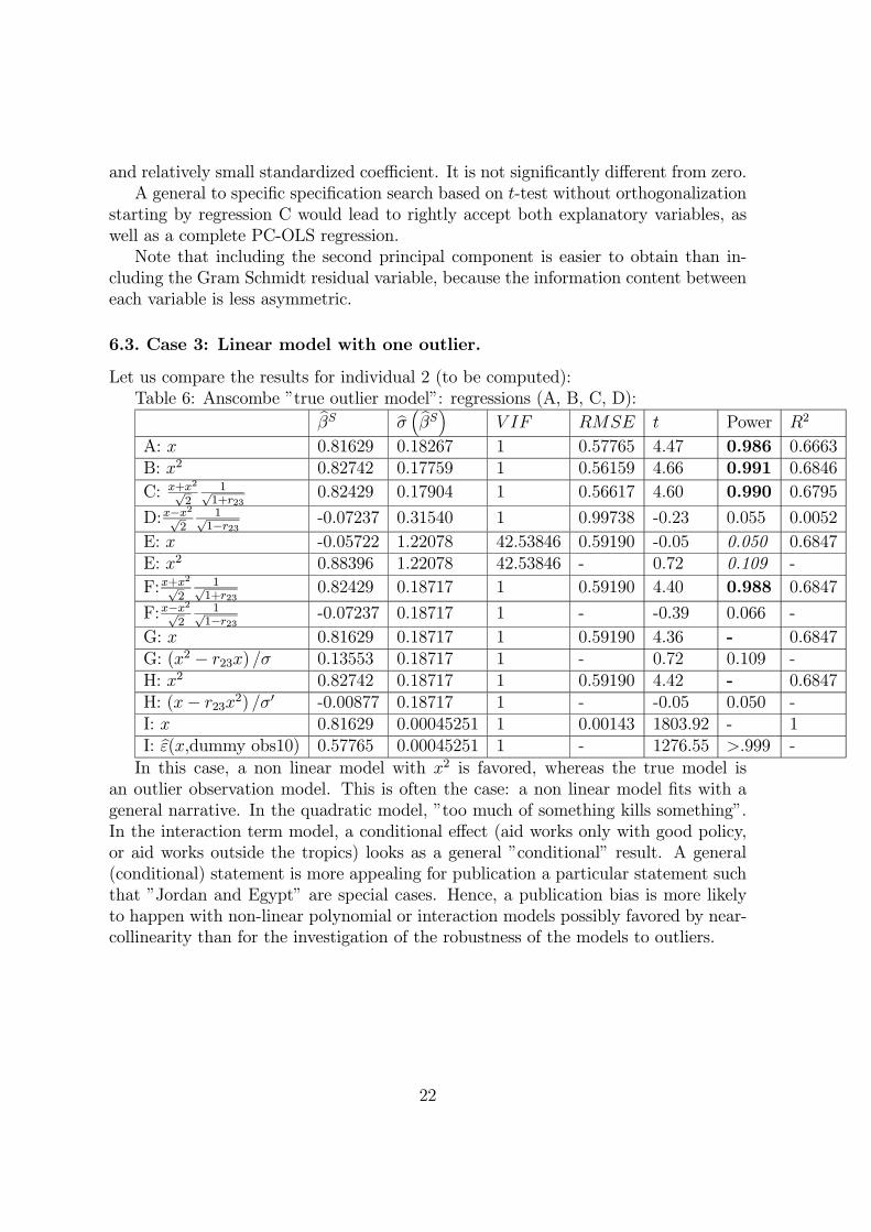
6.3. Case 3: Linear model with one outlier.
Let us compare the results for individual 2 (to be computed):Table 6: Anscombe ”true outlier model”: regressions (A, B, C, D):bβS bσ ³ bβS´ V IF RMSE t Power R2
A: x 0.81629 0.18267 1 0.57765 4.47 0.986 0.6663B: x2 0.82742 0.17759 1 0.56159 4.66 0.991 0.6846
C: x+x2
√2
1√1+r23
0.82429 0.17904 1 0.56617 4.60 0.990 0.6795
D:x−x2
√2
1√1−r23 -0.07237 0.31540 1 0.99738 -0.23 0.055 0.0052
E: x -0.05722 1.22078 42.53846 0.59190 -0.05 0.050 0.6847E: x2 0.88396 1.22078 42.53846 - 0.72 0.109 -
F:x+x2
√2
1√1+r23
0.82429 0.18717 1 0.59190 4.40 0.988 0.6847
F:x−x2
√2
1√1−r23 -0.07237 0.18717 1 - -0.39 0.066 -
G: x 0.81629 0.18717 1 0.59190 4.36 - 0.6847G: (x2 − r23x) /σ 0.13553 0.18717 1 - 0.72 0.109 -H: x2 0.82742 0.18717 1 0.59190 4.42 - 0.6847H: (x− r23x2) /σ0 -0.00877 0.18717 1 - -0.05 0.050 -I: x 0.81629 0.00045251 1 0.00143 1803.92 - 1I: bε(x,dummy obs10) 0.57765 0.00045251 1 - 1276.55 >.999 -
In this case, a non linear model with x2 is favored, whereas the true model isan outlier observation model. This is often the case: a non linear model fits with ageneral narrative. In the quadratic model, ”too much of something kills something”.In the interaction term model, a conditional effect (aid works only with good policy,or aid works outside the tropics) looks as a general ”conditional” result. A general(conditional) statement is more appealing for publication a particular statement suchthat ”Jordan and Egypt” are special cases. Hence, a publication bias is more likelyto happen with non-linear polynomial or interaction models possibly favored by near-collinearity than for the investigation of the robustness of the models to outliers.
22

6.4. Case 4: Quadratic model with near zero bivariate effects and large andprecise trivariate effects
The dependent variable is now the standardized residual x1− r12x2 from case 2. Thisresidual has a zero sample correlation with the variable x2.Table 7: Quadratic model with near zero bivariate effects and large and precise
trivariate effects bβS bσ ³ bβS´ V IF RMSE t Power R2
A: x 0 0.31623 1 1.00000 0.00 0B: x2 -0.15332 0.31249 1 0.98818 -0.49 0.0235
C: x+x2
√2
1√1+r23
-0.07689 0.31529 1 0.99704 -0.24 0.0059
D:x−x2
√2
1√1−r23 0.99704 0.02432 1 0.07690 41.00 0.9941
E: (x2 − r23x) /σ -1 0.00040303 1 0.00127 -2481.2 1F: (x− r23x2) /σ0 0.98818 0.04849 1 0.15333 20.38 0.9765G1: x 6.44503 0.00277 42.53846 0.00134 2326.03 1G2: x2 -6.52215 0.00277 42.53846 - -2353.9 -
H1:x+x2
√2
1√1+r23
-0.07689 0.00042483 1 0.00134 -180.99 1
H2:x−x2
√2
1√1−r23 0.99704 0.00042483 1 - 2346.89 -
I1: x 0 0.00042483 1 0.00134 0.00 - 1I2: (x2 − r23x) /σ -1 0.00042483 1 - -2353.9 -J1: x2 -0.15332 0.00042483 1 0.00134 -360.90 - 1J2: (x− r23x2) /σ0 0.98818 0.00042483 1 - 2326.03 -In this case, simple regression effects are zero or small. However, because r12−r13 is
relatively large so that det (R3) = 0, the trivariate model leads to a perfect correlation.It nonetheless casts doubts on a few non linear models (square or interaction term)
where one of the variable has a near zero correlation with the dependent variable(r12 ≈ 0), such as in the growth and aid/gdp literature (Doucouliagos and Paldam[2008]). With data mining trying a dozen of interacting variable with x2, it is possibleto find an interaction term x4 variable such that x3 = x4x2 such that: r12− r13 > 0.05which may be sufficiently large to turn a near zero effect in bivariate regression as alarge trivariate effect in a precise trivariate regression with near-multicollinearity.- The variable x3−r23x2 is exactly negatively correlated with the dependent variable
x1 − r12x2 (the partial correlation of x3 and x1 is equal to unity in Anscombe’s case2).- The PC-OLS leads to focus on the second principal component, which represents
the smallest part of the variance (0.6%) of the couple of explanatory variables (x2, x3),but explains 99.4% of the variance of the dependent variable x1.- The hierarchical orthogonalization second term has the explains most part of the
variance. As r23 is close to unity, x2 − r23x is close to the difference x2 − x.
- As a consequence, orthogonalization reveals an odd property (the second compo-nents turns to be the most significant effect in the regression).
23

- The powers of the t-test is very large for both variables in the trivariate regression,whereas it is close to zero in the bivariate regressions.However, as seen in the next section, the ”ceteris paribus” interpretation in case
of multicollinearity is not valid.In this case, the results to be chosen depend on substantive meaning. Has the
difference between the variable x−x2 a substantive meaning, despite that it representsonly 0.6% of the variance of the group of explanatory variables? Are the variations ofthe variable x− x2 due to outliers?
6.5. The “Ceteris Paribus” interpretation of parameters is not correct forprecise regressions with near-multicollinearity
Verbeek [2000] states: “xxx”.In case 2 and case 4, the standardized parameters are over unity and very large.
When one omits the variable x22, there is a very large omitted variable bias on theestimated parameter β12:
β12 − r12 = 4.5411− 0.81625 = 3.7249r12 − r13r231− r223
− r12 = −r13 − r12r231− r223
r23 = −β13r32
= − · (−3.7694) · 0.98818
The ”ceteris paribus” (”all other things being equal”, that is: ”the other regressorbeing fixed”) sensitivity of the explained variable with respect to a SINGLE regressoris not valid in this multiple regression with near-collinearity. When the first regressorsmoves from one standard error from the mean x2 + σx2 , the second regressor deviatesfrom its mean with nearly one standard error x3 + 0.98818σx3. Then, the explainedvariable deviation due to a shock of x2+σx2 boils down to the simple regression effectwith a more reliable predicted value of bx1:
bx1 = x1 + (4.5411− 3.7694 · 0.98818)σx1 = x1 + 0.81625σx1Strictly speaking, the ”ceteris paribus” interpretation is only exactly valid when
the regressors are orthogonals.Indeed, here, the second regressor is explicitly the square of the first regressor, so
that nobody falls into the error of the ”ceteris paribus” interpretation. However, whenthe regressors are not explicitly written as a function of each other while facing near-collinearity, many applied researcher still interpret their parameter with the ”ceterisparibus” assumption (all other factors being unchanged). In particular, standardizedparameters over 2 should NEVER be interpreted as a ”ceteris paribus” effect. If x1and x2 are normally distributed:
]−∞, x2 − σ2[S]x2 + σ2,+∞[
33% observations of x2
→]−∞, x1 − 2σ1[S]x1 + 2σ1,+∞[
Predictions of x1 in 5% extreme tails
24
One third of the observations of x2 implies extreme predictions of bx1 in the 5%tails of the distribution of x1. These are unreliable ”catastrophic” forecasts.However, the fact that, because near-collinearity, the Ceteris Paribus interpretation
is not valid does not mean that the regression is not relevant. Both parameters areprecisely estimated because the residuals, their sum of squares and the root meansquare error are close to zero: it more than offsets the rise of variance due to near-collinearity via the VIF when computing the estimated standard error of the estimatedparameters.With this respect, Buse [1984] omitted variable bias interpretation is correct. How-
ever, the ceteris paribus interpretation is not valid, whereas in the Gram Schmidtorthogonalization, the ceteris paribus interpretation on the coefficient of x is correct.Back to the original parameters is always possible, even with incomplete PC-OLS.
6.6. “Near Spurious” regressions in practice
When revisiting the omitted variables argument, Spanos [2006] considered severalcases with ”spurious” omitted variable bias. In the trivariate case, when the nullhypothesis of a zero correlation coefficient between the dependent variable x1 and theregressor x2 (H0 : r12 = 0) is accepted, one can infer (with the addition of a severetesting procedure, see Spanos [2006]) that the relationship between x1 and x2 in asimple regression model is spurious. When the textbook test of the null hypothesisof the omitted variable bias β12 − r12 = −r23r13
1−r223= 0 is rejected, it can be misleading,
because “the difference β12−r12 should not be interpreted as indicating the presence ofconfounding, but the result of a spurious relationship between the dependent variablex1 and the regressor x2” (Spanos [2006]).Conversely, when the null hypothesis of a zero correlation coefficient between the
dependent variable x1 and the other regressor x3 (H0 : r13 = 0) is accepted, one caninfer (with the addition of a severe testing procedure) that the relationship between x1and x3 in a simple regression model is spurious. When the null hypothesis r12 = 0 andr23 = 0 are rejected, the textbook test of the null hypothesis of the omitted variable
bias β12 − r12 = r121−r223
− r12 = r12 ·³
r2231−r223
´= 0 is rejected, it can be misleading,
because “the difference β12−r12 should not be interpreted as indicating the presence ofconfounding. In reality, x3 has no role to play in establishing the ”true” relationshipbetween the dependent variable x1 and the regressor x2, since there is no relationshipbetween the dependent variable x1 and the other regressor x3” (Spanos [2006]).In practice, in order to avoid ”near spurious” regressions, an applied researcher
could remove all regressors such that the null composite hypothesis H0 : r1j < 0.1(for positive sample correlation coefficients) or H0 : r1j > −0.1 (for sample negativecoefficients) at the beginning of his multiple regression specification search, in partic-ular, when it is a general to specific selection of regressors. The thresholds |0.1| implythat the true correlation coefficient should explain at least 1% of the variance of thedependent variable in a simple correlation model (the coefficient of determination is
25
such that: R21.j > 1%). It refers to Cohen [1988] classification of effects in his overallevaluation of the power of tests for cross sections: r1j = 0.1 or r
21j = 1%: small effect,
r1j = 0.3 or r21j = 9% medium size effect, r1j = 0.5 or r
21j = 25% large effect. This
test is based on Fisher’s Z transform available in many statistical software computingcorrelation matrix. For example, using SAS software, the instruction is: “proc corrdata=database fischer (rho0=0.1 lower);”. One may also apply Mayo and Spanos[2006] severe testing procedure, which is more restrictive.In a second step, he may look for stratification (Hendry and Nielsen [2008]), that
is finding subsets of observations (defined by a dummy variable 1subset) such that|r (x1, x2 · 1subset)| ≥ 0.1 for the excluded variables such that |r (x1, x2)| ≤ 0.1. Thisdummy variable for the selection of observations may be itself endogenous and maydepend on variables zj, or on the variable x2 itself (quadratic model) so that interactionterms may matter |r (x1, x2 · zj)| ≥ 0.1 as well. The key point is to exclude x2 inthe general model before the general to specific selection of regressors, so that theinteraction terms x2 · zj does not turn to be significantly different from zero due tothe near-collinearity regression.An applied researcher may evaluate with care whether the selected observations
driving the correlation r (x1, x2 · zj) are only a few observations (outliers): in thiscase the initial robust selection of observations is likely to perform much better:r (x1, x2 · 1subset) > r (x1, x2 · zj). Because sometimes, it may be more interesting tofind general results than stating particular cases, one may be tempted to favor regres-sions with x2 · zj becausethey are ”general conditional effect”, despite the fact thatthey are not robust to the removal of a few outliers. As shown in Roodman [2008]example: an editor would favour a general conditional argument ”aid is correlatedwith growth for non tropical countries” than ”large aid/gdp with high growth rate isfound in Jordan, Egypt and Botswana”.
7. Conclusion
This note presented orthogonalized regressors and constrained estimations. Present-ing the correlation matrix including the explained variable, the VIF and the confi-dence interval of each estimated parameters, discussing the plausibility of the sizeof the (standardized) parameters and explaining the data generating process of thecollinearity between regressors is useful.
References
[1] Anscombe A. [1973]. Graphs in Statistical Analysis. American Statistician, 27,pp. 17-21.
[2] Buse A. [1994]. Brickmaking and the collinear arts: a cautionary tale. CanadianJournal of Economics. Revue Canadienne d’Economie. 27(2), pp.408-414.
26
[3] Castle J. [2008]. Econometric Model Selection: Nonlinear Techniques and Fore-casting, Saarbruumlcken: VDM Verlag. ISBN: 978-3-639-00458-8
[4] Castle J. and Hendry D. [2008]. A Low-Dimension Portmanteau Test for Non-linearity (with David F. Hendry), Working paper No. 326, Economics Depart-ment, University of Oxford.
[5] Castle J. and Hendry D. [2008]. Extending the Boundaries of Automatic ModelSelection: Non-linear Models’, Working paper, Economics Department, Univer-sity of Oxford.
[6] Cohen [1988]. Statistical Power Analysis for the Behavioral Sciences.
[7] Doucouliagos H. and Paldam M. [2009]. The aid effectiveness literature: Thesad results of 40 years of research. Journal of Economic Surveys, forthcoming.Working paper, M. Paldam’s webpage.
[8] Greene W.H. [2000]. Econometric analysis. Fourth edition.
[9] Hendry D.F. and Nielsen B. [2007]. Econometric Modelling. A Likelihood Ap-proach. Princeton University Press.
[10] Massy W.F. [1965]. Principal Components Regression in Exploratory StatisticalResearch. Journal of the American Statistical Association. 20(309), pp.234-256.
[11] Puntanen S. and Styan G.P.H. [2005]. Schur complements in statistics and prob-ability. In The Schur complement and its applications, F. Zhang editor, SpringerVerlag, pp. 163-226.
[12] Roodman D. [2008]. Through the Looking Glass, and What OLS Found There:On Growth, Foreign Aid, and Reverse Causality. Center for Global DevelopmentWorking Paper Number 137.
[13] Spanos A. and McGuirk A. [2002]. The Problem of near-multicollinearity revis-ited: erratic vs systematic volatility. Journal of Econometrics, 108, 365-393.
[14] Spanos [2006]. Revisiting the omitted variables argument: Substantive vs. statis-tical adequacy. Journal of Economic Methodology, Volume 13, Issue 2, pages 179- 218
[15] Stanley, T.D., [2005]. Beyond publication bias. Journal of Economic Surveys 19,309-45.
[16] Paper on selecting variables versus t statistics. SAS
27
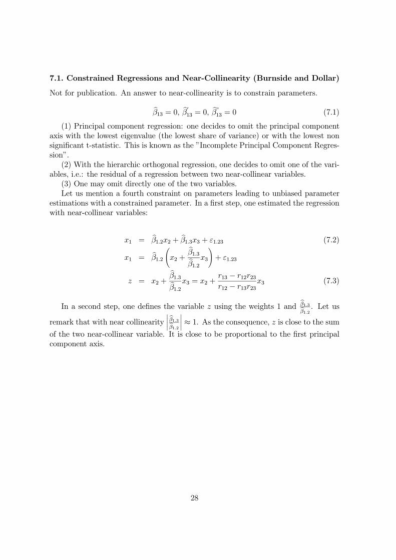
7.1. Constrained Regressions and Near-Collinearity (Burnside and Dollar)
Not for publication. An answer to near-collinearity is to constrain parameters.
bβ13 = 0, bβ013 = 0,
bβ”13 = 0 (7.1)
(1) Principal component regression: one decides to omit the principal componentaxis with the lowest eigenvalue (the lowest share of variance) or with the lowest nonsignificant t-statistic. This is known as the ”Incomplete Principal Component Regres-sion”.(2) With the hierarchic orthogonal regression, one decides to omit one of the vari-
ables, i.e.: the residual of a regression between two near-collinear variables.(3) One may omit directly one of the two variables.Let us mention a fourth constraint on parameters leading to unbiased parameter
estimations with a constrained parameter. In a first step, one estimated the regressionwith near-collinear variables:
x1 = bβ1.2x2 + bβ1.3x3 + ε1.23 (7.2)
x1 = bβ1.2Ãx2 +
bβ1.3bβ1.2x3!+ ε1.23
z = x2 +bβ1.3bβ1.2x3 = x2 +
r13 − r12r23r12 − r13r23
x3 (7.3)
In a second step, one defines the variable z using the weights 1 andbβ1.3bβ1.2 . Let us
remark that with near collinearity¯ bβ1.3bβ1.2
¯≈ 1. As the consequence, z is close to the sum
of the two near-collinear variable. It is close to be proportional to the first principalcomponent axis.
28