Energies 2017, 10, 514; doi:10.3390/en10040514 www.mdpi.com/journal/energies

Article

Generalized Energy Flow Analysis Considering Electricity Gas and Heat Subsystems in Local-Area Energy Systems Integration Jiaqi Shi 1,*, Ling Wang 2, Yingrui Wang 3 and Jianhua Zhang 1

1 State Key Laboratory of New Energy Power System, North China Electric Power University, Beijing 102206, China; jhzhang001@ncepu.edu.cn

2 School of Information Science and Engineering, Shenyang Ligong University, Shenyang 110159, China; lowang@163.com

3 China Energy Engineering Group Tianjin Electric Power Design Institute Co., Ltd., Tianjin 300400, China; yingruiw@126.com

* Correspondence: phdshijiaqi@foxmail.com; Tel.: +86-010-6177-3855

Academic Editor: Ali Elkamel Received: 19 January 2017; Accepted: 5 April 2017; Published: 10 April 2017

Abstract: To alleviate environmental pollution and improve the efficient use of energy, energy systems integration (ESI)—covering electric power systems, heat systems and natural gas systems—has become an important trend in energy utilization. The traditional power flow calculation method, with the object as the power system, will prove difficult in meeting the requirements of the coupled energy flow analysis. This paper proposes a generalized energy flow (GEF) analysis method which is suitable for an ESI containing electricity, heat and gas subsystems. First, the models of electricity, heat, and natural gas networks in the ESI are established. In view of the complexity of the conventional method to solve the gas network including the compressor, an improved practical equivalent method was adopted based on different control modes. On this basis, a hybrid method combining homotopy and the Newton-Raphson algorithm was executed to compute the nonlinear equations of GEF, and the Jacobi matrix reflecting the coupling relationship of multi-energy was derived considering the grid connected mode and island modes of the power system in the ESI. Finally, the validity of the proposed method in multi-energy flow calculation and the analysis of interacting characteristics was verified using practical cases.

Keywords: energy systems integration (ESI); generalized energy flow (GEF); compressor; homotopy; Newton-Raphson; grid connected mode and island mode

1. Introduction

The energy industry has gone through great change due to the rapid development of technology and the economy in the 21st century. In recent years, fossil energy exhaustion, environmental pollution, large-scale renewable energy application, etc. have proven to be key drivers in the development of a modern energy system which needs to meet the requirements of low-carbon emissions and efficient utilization of friendly sustainable energy sources. However, different energy systems are designed, planning and operating independently of the traditional style, which separates the coupling correlations between different types of energy and largely limits the flexibility of the energy system. In this case, ESI is proposed as it is an important type of new energy system, and covers electric power, heat and natural gas systems with the purpose of coordinating the whole system in the processes of generation, transmission and consumption, which are considered to be the core technology of the “third industrial revolution” [1]. Therefore, the development of an integrated modeling and analysis framework for ESI represents an essential need for future research.

Energies 2017, 10, 514 2 of 17

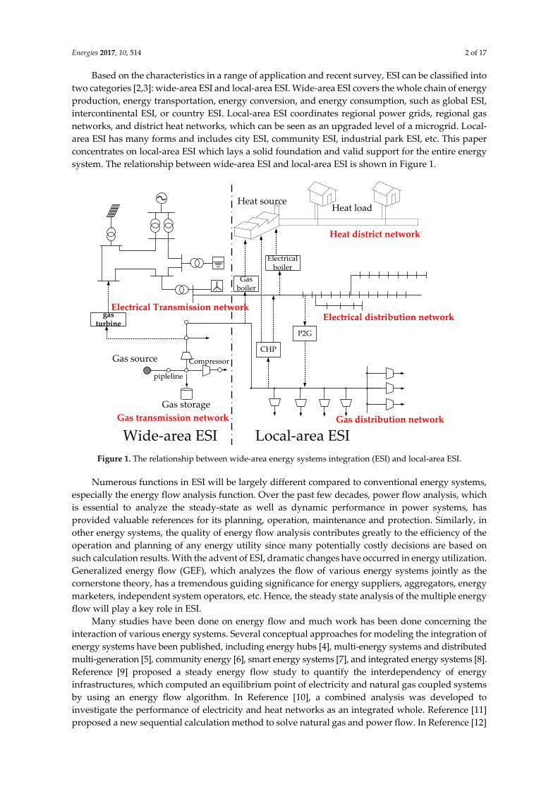
Based on the characteristics in a range of application and recent survey, ESI can be classified into two categories [2,3]: wide-area ESI and local-area ESI. Wide-area ESI covers the whole chain of energy production, energy transportation, energy conversion, and energy consumption, such as global ESI, intercontinental ESI, or country ESI. Local-area ESI coordinates regional power grids, regional gas networks, and district heat networks, which can be seen as an upgraded level of a microgrid. Local-area ESI has many forms and includes city ESI, community ESI, industrial park ESI, etc. This paper concentrates on local-area ESI which lays a solid foundation and valid support for the entire energy system. The relationship between wide-area ESI and local-area ESI is shown in Figure 1.

gas turbine

CHP

P2G

Electrical Transmission networkElectrical distribution network

Gas transmission network

Compressor

pipleline

Gas storage

Wide-area ESI Local-area ESI

Electricalboiler

Heat district network

Gasboiler

Gas distribution network

Heat sourceHeat load

Gas source

Figure 1. The relationship between wide-area energy systems integration (ESI) and local-area ESI.

Numerous functions in ESI will be largely different compared to conventional energy systems, especially the energy flow analysis function. Over the past few decades, power flow analysis, which is essential to analyze the steady-state as well as dynamic performance in power systems, has provided valuable references for its planning, operation, maintenance and protection. Similarly, in other energy systems, the quality of energy flow analysis contributes greatly to the efficiency of the operation and planning of any energy utility since many potentially costly decisions are based on such calculation results. With the advent of ESI, dramatic changes have occurred in energy utilization. Generalized energy flow (GEF), which analyzes the flow of various energy systems jointly as the cornerstone theory, has a tremendous guiding significance for energy suppliers, aggregators, energy marketers, independent system operators, etc. Hence, the steady state analysis of the multiple energy flow will play a key role in ESI.

Many studies have been done on energy flow and much work has been done concerning the interaction of various energy systems. Several conceptual approaches for modeling the integration of energy systems have been published, including energy hubs [4], multi-energy systems and distributed multi-generation [5], community energy [6], smart energy systems [7], and integrated energy systems [8]. Reference [9] proposed a steady energy flow study to quantify the interdependency of energy infrastructures, which computed an equilibrium point of electricity and natural gas coupled systems by using an energy flow algorithm. In Reference [10], a combined analysis was developed to investigate the performance of electricity and heat networks as an integrated whole. Reference [11] proposed a new sequential calculation method to solve natural gas and power flow. In Reference [12]

Energies 2017, 10, 514 3 of 17

the concept of a probabilistic load flow, which has been widely applied in electric power systems, was extended to probabilistic energy flow analysis including electric power and natural gas flows. In addition to steady energy flow, plenty of studies have focused on optimal energy flow studies. In References [4,13], the optimal energy flow was solved by the centralized optimization algorithm and the distributed optimization algorithm, respectively, based on the energy hub concept. Reference [14] suggested a multi-objective algorithm to optimize its energy flow by considering the dynamics of the system and the equipment’s thermal inertias. With respect to nonlinear algebraic equation solutions, one standard approach of solving the algorithm is the Newton-Raphson method [15]. However, traditional power flow relying on Newton-Raphson is not robust if no starting point sufficiently close to a solution is provided. To address this issue, several methods were developed to reliably compute nonlinear equations, such as the Gauss Seidel iterations method [16], and the homotopy-enhanced method [17]; however, their convergence rate was relatively limited. Therefore, the improvement of existing approaches is still an urgent problem to be solved regardless of the mathematical model or solution algorithm.

By taking account of current scientific research and the engineering applications of ESI, the contributions of this paper can be summarized in three aspects as follows:

(1) To the best of our knowledge, most previous research has concentrated either on the interaction of electricity-gas or electricity-heat. In this paper, the GEF of a local-area ESI is proposed, which designs the whole energy flow framework of gas, heat, and electricity jointly.

(2) Complicated nonlinear mathematical models of some devices in energy systems create dilemmas in the implementation of energy flow calculations, especially regarding the compressor facility that belongs to gas energy system. By considering that issue, we effectively simplified the model as an equivalent transformation which reduces computational complexity.

(3) By considering the advantage of the algorithm and the complexity of the ESI model, a hybrid algorithm, which combines the homotopy method and Newton's method, was adopted to solve nonlinear equations of GEF.

This paper is organized as follows. Section 2 presents the fundamental concept and mathematic model of each energy subsystem. Section 3 describes the GEF calculation method based on homotopy and the Newton-Raphson algorithm, and the Jacobi matrix, which maps multi-energy coupling relationships, is proposed. Section 4 shows the experimental results used to verify the effectiveness of the proposed algorithm in different scenarios. Finally, our conclusions and future research avenues are given in Section 5.

2. Generalized Energy Flow Model

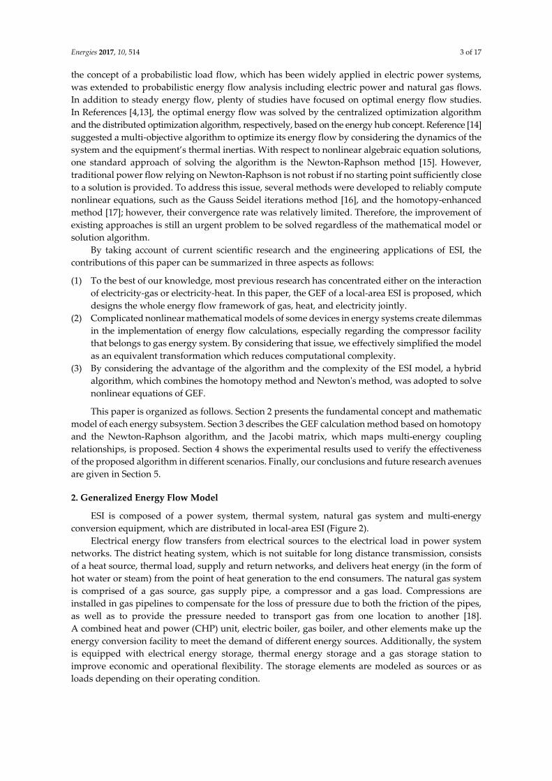
ESI is composed of a power system, thermal system, natural gas system and multi-energy conversion equipment, which are distributed in local-area ESI (Figure 2).

Electrical energy flow transfers from electrical sources to the electrical load in power system networks. The district heating system, which is not suitable for long distance transmission, consists of a heat source, thermal load, supply and return networks, and delivers heat energy (in the form of hot water or steam) from the point of heat generation to the end consumers. The natural gas system is comprised of a gas source, gas supply pipe, a compressor and a gas load. Compressions are installed in gas pipelines to compensate for the loss of pressure due to both the friction of the pipes, as well as to provide the pressure needed to transport gas from one location to another [18]. A combined heat and power (CHP) unit, electric boiler, gas boiler, and other elements make up the energy conversion facility to meet the demand of different energy sources. Additionally, the system is equipped with electrical energy storage, thermal energy storage and a gas storage station to improve economic and operational flexibility. The storage elements are modeled as sources or as loads depending on their operating condition.

Energies 2017, 10, 514 4 of 17

Figure 2. Architecture of local-area ESI.

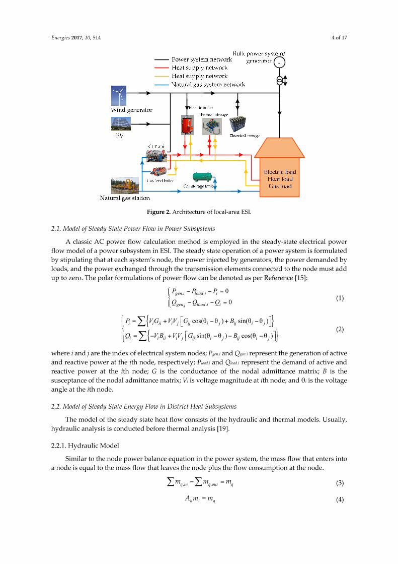
2.1. Model of Steady State Power Flow in Power Subsystems

A classic AC power flow calculation method is employed in the steady-state electrical power flow model of a power subsystem in ESI. The steady state operation of a power system is formulated by stipulating that at each system’s node, the power injected by generators, the power demanded by loads, and the power exchanged through the transmission elements connected to the node must add up to zero. The polar formulations of power flow can be denoted as per Reference [15]:

.

. .

.

0

0i

gen i load i i

gen load i i

P P P

Q Q Q

(1)

cos(θ θ ) sin(θ θ )

sin(θ θ ) cos(θ θ )

i i ii i j ij i j ij i j

i i ii i j ij i j ij i j

P VG VV G B

Q V B VV G B

(2)

where i and j are the index of electrical system nodes; Pgen.i and Qgen.i represent the generation of active and reactive power at the ith node, respectively; Pload.i and Qload.i represent the demand of active and reactive power at the ith node; G is the conductance of the nodal admittance matrix; B is the susceptance of the nodal admittance matrix; Vi is voltage magnitude at ith node; and θi is the voltage angle at the ith node.

2.2. Model of Steady State Energy Flow in District Heat Subsystems

The model of the steady state heat flow consists of the hydraulic and thermal models. Usually, hydraulic analysis is conducted before thermal analysis [19].

2.2.1. Hydraulic Model

Similar to the node power balance equation in the power system, the mass flow that enters into a node is equal to the mass flow that leaves the node plus the flow consumption at the node.

, ,q in q out qm m m (3)

h i qA m = m (4)

Energies 2017, 10, 514 5 of 17

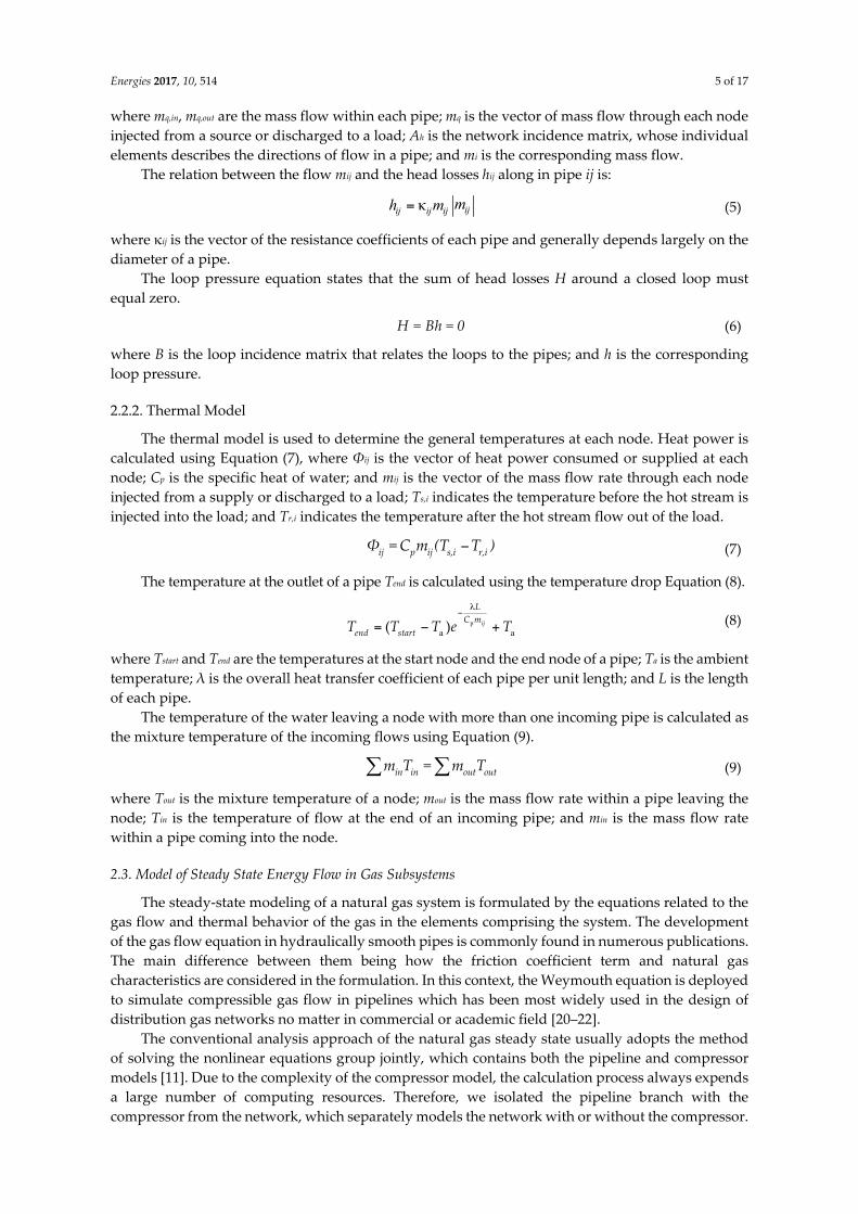
where mq,in, mq,out are the mass flow within each pipe; mq is the vector of mass flow through each node injected from a source or discharged to a load; Ah is the network incidence matrix, whose individual elements describes the directions of flow in a pipe; and mi is the corresponding mass flow.

The relation between the flow mij and the head losses hij along in pipe ij is:

κ ijij ij ij mh m (5)

where κij is the vector of the resistance coefficients of each pipe and generally depends largely on the diameter of a pipe.

The loop pressure equation states that the sum of head losses H around a closed loop must equal zero.

H = Bh = 0 (6)

where B is the loop incidence matrix that relates the loops to the pipes; and h is the corresponding loop pressure.

2.2.2. Thermal Model

The thermal model is used to determine the general temperatures at each node. Heat power is calculated using Equation (7), where Φij is the vector of heat power consumed or supplied at each node; Cp is the specific heat of water; and mij is the vector of the mass flow rate through each node injected from a supply or discharged to a load; Ts,i indicates the temperature before the hot stream is injected into the load; and Tr,i indicates the temperature after the hot stream flow out of the load.

ij p ij s,i r,iΦ = C m (T T ) (7)

The temperature at the outlet of a pipe Tend is calculated using the temperature drop Equation (8).

p

a a( ) ij

LC m

end startT T T e T

(8)

where Tstart and Tend are the temperatures at the start node and the end node of a pipe; Ta is the ambient temperature; λ is the overall heat transfer coefficient of each pipe per unit length; and L is the length of each pipe.

The temperature of the water leaving a node with more than one incoming pipe is calculated as the mixture temperature of the incoming flows using Equation (9).

in in out outm T = m T (9)

where Tout is the mixture temperature of a node; mout is the mass flow rate within a pipe leaving the node; Tin is the temperature of flow at the end of an incoming pipe; and min is the mass flow rate within a pipe coming into the node.

2.3. Model of Steady State Energy Flow in Gas Subsystems

The steady-state modeling of a natural gas system is formulated by the equations related to the gas flow and thermal behavior of the gas in the elements comprising the system. The development of the gas flow equation in hydraulically smooth pipes is commonly found in numerous publications. The main difference between them being how the friction coefficient term and natural gas characteristics are considered in the formulation. In this context, the Weymouth equation is deployed to simulate compressible gas flow in pipelines which has been most widely used in the design of distribution gas networks no matter in commercial or academic field [20–22].

The conventional analysis approach of the natural gas steady state usually adopts the method of solving the nonlinear equations group jointly, which contains both the pipeline and compressor models [11]. Due to the complexity of the compressor model, the calculation process always expends a large number of computing resources. Therefore, we isolated the pipeline branch with the compressor from the network, which separately models the network with or without the compressor.

Energies 2017, 10, 514 6 of 17

Specifically, the gas flow considering the pipeline with the compressor can be calculated directly by the method we employed which regards the two terminal nodes of the branch with the compressor as the equivalent load. This approach results in the mathematical model of the compressor no longer being involved in the network calculation, which greatly simplifies the calculation process.

2.3.1. Natural Gas Network Model without Compressor

The model without compressor is usually used to describe the relationship between the nodal pressure and the pipeline flow in the natural gas network. The steady state flow fr of the natural gas pipeline r can be defined as:

θ Δ 2 2 2r r r ij ij i jf = ( p ) = K s s (p - p ) (10)

16/3

1389640

ij a ar

ij

l T GZK

D (11)

where Kr is the pipeline constant; Δpr2 = pi2 − pj2 represents the pressure drop of pipeline r; sij is used to characterize the flow direction of natural gas, when pi > pj, sij is +1, otherwise −1. Dij is diameter of the pipeline between node i and j. lij is the length of the pipeline between i and j. Za is the average compressibility factor; Ta is average temperature of natural gas; and G is gas relative density.

The flow continuity equation of the natural gas network is expressed as:

gA f = L (12)

where Ag is the node-branch incidence matrix of the natural gas network without the pipeline containing the compressor; f indicates the pipeline natural gas flow; L indicates the flow of each node Πi = pi2, ΔΠr = Δpr2, then the pressure drop vector of the natural gas pipeline are noted as:

Δ TgΠ = -A Π (13)

2.3.2. Natural Gas Flow Calculation Method with the Compressor

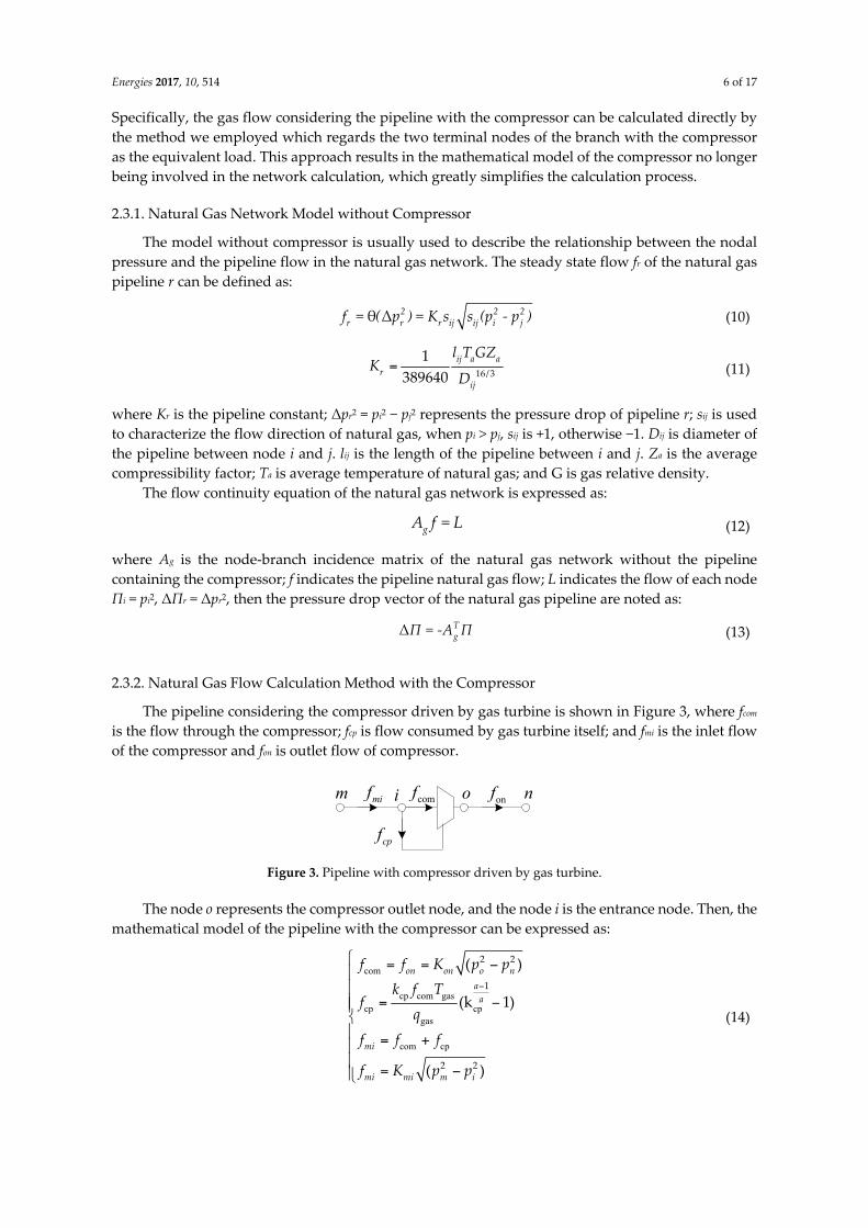
The pipeline considering the compressor driven by gas turbine is shown in Figure 3, where fcom is the flow through the compressor; fcp is flow consumed by gas turbine itself; and fmi is the inlet flow of the compressor and fon is outlet flow of compressor.

m ncomf

cpf

oimif onf

Figure 3. Pipeline with compressor driven by gas turbine.

The node o represents the compressor outlet node, and the node i is the entrance node. Then, the mathematical model of the pipeline with the compressor can be expressed as:

com

cp com gascp cp

gas

com cp

2 2

1

2 2

( )

(k 1)

( )

on on o na

a

mi

mi mi m i

f f K p pk f T

fq

f f f

f K p p

(14)

Energies 2017, 10, 514 7 of 17

where kcp is the compression ratio; Kmi, Kon are constants of the inlet and outlet pipes; pm, pn, pi, po are the correspondent nodal pressure; qgas is the natural gas heating value; Tgas is the natural gas temperature; and a is the polytropic exponent.

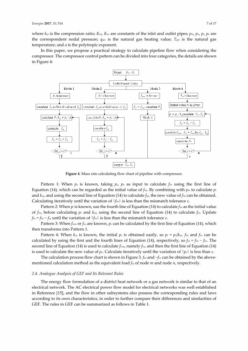
In this paper, we propose a practical strategy to calculate pipeline flow when considering the compressor. The compressor control pattern can be divided into four categories, the details are shown in Figure 4:

,m np p

op

onf

ip cp, /o ik p p

cpf

cpmi onf f f

?mif

ip

op cp, /o ik p p

cpf

cpon mif f f

?onf

comf

op

cpk

op

cp/i op p k ,on mif f

cp mi onf f f

cp cpf k、com com, onf f f

op

?op

,mi onf f

mif com ,onf fmif onf

Figure 4. Mass rate calculating flow chart of pipeline with compressor.

Pattern 1: When po is known, taking po, pn as input to calculate fon using the first line of Equation (14), which can be regarded as the initial value of fmi. By combining with pm to calculate pi and kcp, and using the second line of Equation (14) to calculate fcp, the new value of fmi can be obtained. Calculating iteratively until the variation of |fmi| is less than the mismatch tolerance ε.

Pattern 2: When pi is known, use the fourth line of Equation (14) to calculate fmi as the initial value of fon, before calculating po and kcp, using the second line of Equation (14) to calculate fcp. Update fon = fmi − fcp until the variation of |fon| is less than the mismatch tolerance ε.

Pattern 3: When fcom or fon are known, po can be calculated by the first line of Equation (14), which then transforms into Pattern 1.

Pattern 4: When kcp is known, the initial po is obtained easily, so pi = po/kcp. fmi and fon can be calculated by using the first and the fourth lines of Equation (14), respectively, so fcp = fmi − fon. The second line of Equation (14) is used to calculate fcom, namely fon, and then the first line of Equation (14) is used to calculate the new value of po. Calculate iteratively until the variation of |po| is less than ε.

The calculation process flow chart is shown in Figure 3. fmi and −fon can be obtained by the above-mentioned calculation method as the equivalent load feq of node m and node n, respectively.

2.4. Analogue Analysis of GEF and Its Relevant Rules

The energy flow formulation of a district heat network or a gas network is similar to that of an electrical network. The AC electrical power flow model for electrical networks was well established in Reference [15], and the flow in other subsystems also possess the corresponding rules and laws according to its own characteristics, in order to further compare their differences and similarities of GEF. The rules in GEF can be summarized as follows in Table 1.

Energies 2017, 10, 514 8 of 17

Table 1. Analogue analysis of generalized energy flow (GEF) rules and principles.

Energy System Generalized Kirchhoff’s First Law Generalized Kirchhoff’s Second Law

Electrical subsystem Kirchhoff’s current law

I1 + I2…+ In = 0 Kirchhoff’s voltage law

U1 + U2 +…+ Un = 0

Thermal subsystem Continuity of heat flow

m1 + m2 +…mn = 0 Loop pressure equation

h1 + h2 +...+ hn = 0

Natural gas subsystem Continuity of gas flow

f1 + f2 +…+ fn = 0 Loop pressure equation Π1 + Π2 +...+ Πn = 0

3. GEF Calculation Method

Due to the simultaneous equations of different energy systems, the number of nonlinear equations and the dimension of decision variables are greatly increased, therefore, an inappropriate method used to solve the nonlinear equations will lead to bad convergence or even ill-conditioned flow. In this paper, we used a hybrid method to compute the equilibrium point of ESI, which is comprised of the homotopy method and the Newton-Raphson method. First, the homotopy algorithm was used to calculate the initial value of equations by its global convergence superiority, before the Newton-Raphson algorithm was executed to quickly converge to a stable solution, which met both requirements of computational stability and convergence speed.

3.1. GEF Mode

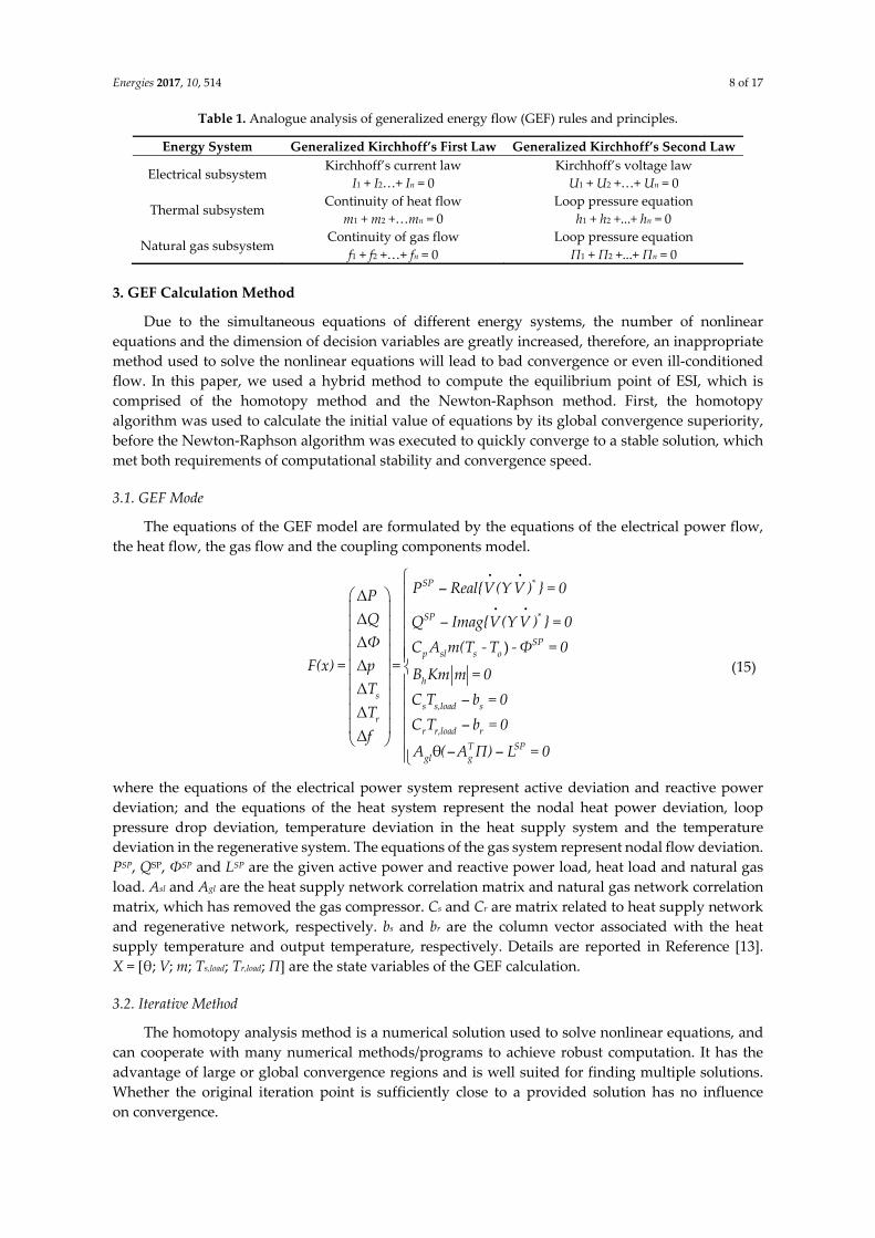
The equations of the GEF model are formulated by the equations of the electrical power flow, the heat flow, the gas flow and the coupling components model.

ΔΔΔ )ΔΔΔΔ

θ

SP *

SP *

SPp sl s o

hs

s s,load sr

r r,load rT SP

gl g

P Real{V(Y V ) } = 0PQ Q Imag{V(Y V ) } = 0Φ C A m(T - T -Φ = 0

F(x) = =p B Km m = 0T

C T b = 0T

C T b = 0f

A ( A Π) L = 0

(15)

where the equations of the electrical power system represent active deviation and reactive power deviation; and the equations of the heat system represent the nodal heat power deviation, loop pressure drop deviation, temperature deviation in the heat supply system and the temperature deviation in the regenerative system. The equations of the gas system represent nodal flow deviation. PSP, QSP, ΦSP and LSP are the given active power and reactive power load, heat load and natural gas load. Asl and Agl are the heat supply network correlation matrix and natural gas network correlation matrix, which has removed the gas compressor. Cs and Cr are matrix related to heat supply network and regenerative network, respectively. bs and br are the column vector associated with the heat supply temperature and output temperature, respectively. Details are reported in Reference [13]. X = [θ; V; m; Ts,load; Tr,load; Π] are the state variables of the GEF calculation.

3.2. Iterative Method

The homotopy analysis method is a numerical solution used to solve nonlinear equations, and can cooperate with many numerical methods/programs to achieve robust computation. It has the advantage of large or global convergence regions and is well suited for finding multiple solutions. Whether the original iteration point is sufficiently close to a provided solution has no influence on convergence.

Energies 2017, 10, 514 9 of 17

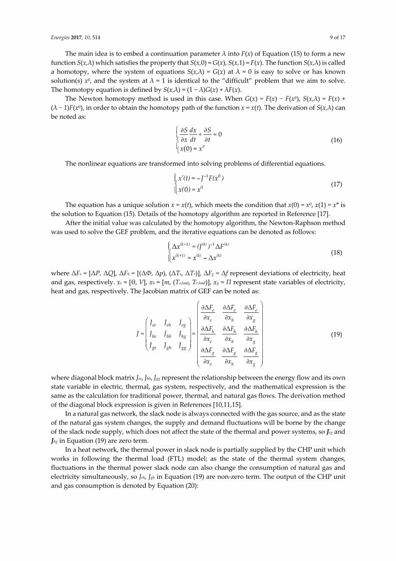
The main idea is to embed a continuation parameter λ into F(x) of Equation (15) to form a new function S(x,λ) which satisfies the property that S(x,0) = G(x), S(x,1) = F(x). The function S(x,λ) is called a homotopy, where the system of equations S(x,λ) = G(x) at λ = 0 is easy to solve or has known solution(s) x0, and the system at λ = 1 is identical to the “difficult” problem that we aim to solve. The homotopy equation is defined by S(x,λ) = (1 − λ)G(x) + λF(x).

The Newton homotopy method is used in this case. When G(x) = F(x) − F(x0), S(x,λ) = F(x) + (λ − 1)F(x0), in order to obtain the homotopy path of the function x = x(t). The derivation of S(x,λ) can be noted as:

0

(0) 0

S dx S+ =x dt t

x = x (16)

The nonlinear equations are transformed into solving problems of differential equations.

1 0

00x (t) = J F(x )x( ) = x

(17)

The equation has a unique solution x = x(t), which meets the condition that x(0) = x0, x(1) = x* is the solution to Equation (15). Details of the homotopy algorithm are reported in Reference [17].

After the initial value was calculated by the homotopy algorithm, the Newton-Raphson method was used to solve the GEF problem, and the iterative equations can be denoted as follows:

1 1

1

Δ ΔΔ

(k+ ) (k) (k)

(k+ ) (k) (k)

x = (J ) Fx = x x

(18)

where ΔFe = [ΔP, ΔQ], ΔFh = [(ΔΦ, Δp), (ΔTs, ΔTr)], ΔFg = Δf represent deviations of electricity, heat and gas, respectively. xe = [θ, V], xh = [m, (Ts,load, Tr,load)], xg = Π represent state variables of electricity, heat and gas, respectively. The Jacobian matrix of GEF can be noted as:

Δ Δ Δ

Δ Δ Δ

Δ Δ Δ

e e e

e h gee eh eg

h h hhe hh hg

e h gge gh gg

g g g

e h g

F F Fx x x

J J JF F F

J = J J J =x x x

J J JF F F

x x x

(19)

where diagonal block matrix Jee, Jhh, Jgg represent the relationship between the energy flow and its own state variable in electric, thermal, gas system, respectively, and the mathematical expression is the same as the calculation for traditional power, thermal, and natural gas flows. The derivation method of the diagonal block expression is given in References [10,11,15].

In a natural gas network, the slack node is always connected with the gas source, and as the state of the natural gas system changes, the supply and demand fluctuations will be borne by the change of the slack node supply, which does not affect the state of the thermal and power systems, so Jeg and Jhg in Equation (19) are zero term.

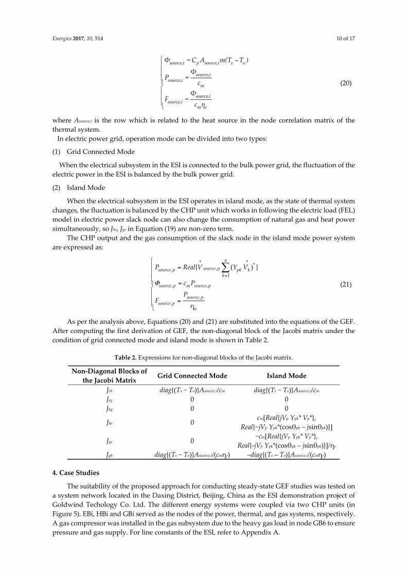
In a heat network, the thermal power in slack node is partially supplied by the CHP unit which works in following the thermal load (FTL) model; as the state of the thermal system changes, fluctuations in the thermal power slack node can also change the consumption of natural gas and electricity simultaneously, so Jeh, Jgh in Equation (19) are non-zero term. The output of the CHP unit and gas consumption is denoted by Equation (20):

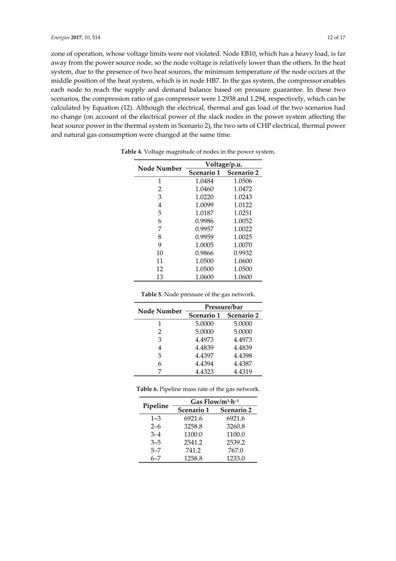
Energies 2017, 10, 514 10 of 17

source,i p source,i s o

source,isource,i

m

source,isource,i

m e

Φ = C A m(T T )

ΦP =

cΦ

F =c η

(20)

where Asource,i is the row which is related to the heat source in the node correlation matrix of the thermal system.

In electric power grid, operation mode can be divided into two types:

(1) Grid Connected Mode

When the electrical subsystem in the ESI is connected to the bulk power grid, the fluctuation of the electric power in the ESI is balanced by the bulk power grid.

(2) Island Mode

When the electrical subsystem in the ESI operates in island mode, as the state of thermal system changes, the fluctuation is balanced by the CHP unit which works in following the electric load (FEL) model in electric power slack node can also change the consumption of natural gas and heat power simultaneously, so Jhe, Jge in Equation (19) are non-zero term.

The CHP output and the gas consumption of the slack node in the island mode power system are expressed as:

*

,,1

, ,

,,

e

{ ( ) }

η

n

source psource p pk kk

source p m source p

source psource p

P Real V Y V

c P

PF

(21)

As per the analysis above, Equations (20) and (21) are substituted into the equations of the GEF. After computing the first derivation of GEF, the non-diagonal block of the Jacobi matrix under the condition of grid connected mode and island mode is shown in Table 2.

Table 2. Expressions for non-diagonal blocks of the Jacobi matrix.

Non-Diagonal Blocks of the Jacobi Matrix

Grid Connected Mode Island Mode

Jeh diag{(Ts − To)}Asource,i/cm diag{(Ts − To)}Asource,i/cm Jeg 0 0 Jhg 0 0

Jhe 0 cm[Real{jVp Ypk* Vp*},

Real{−jVp Ypk*(cosθpk – jsinθpk)}]

Jge 0 −cm[Real{jVp Ypk* Vp*}, Real{-jVp Ypk*(cosθpk – jsinθpk)}]/ηe

Jgh diag{(Ts − To)}Asource,i/(cmηe) –diag{(Ts – To)}Asource,i/(cmηe)

4. Case Studies

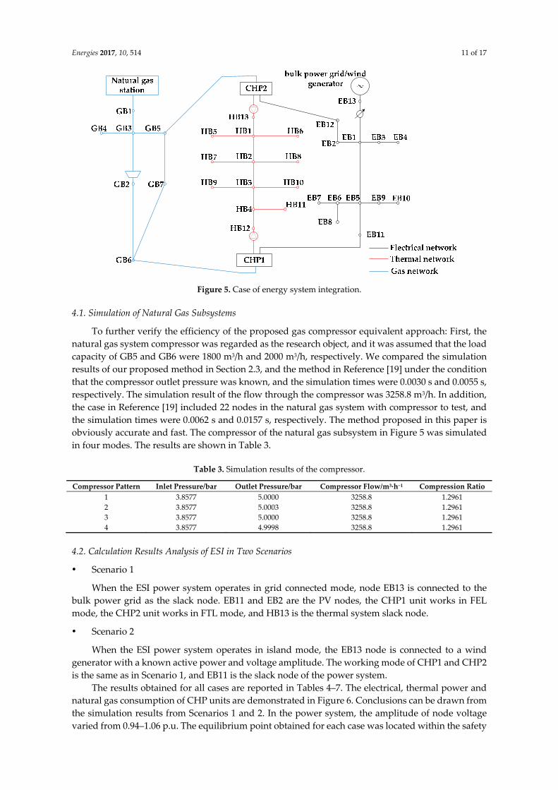
The suitability of the proposed approach for conducting steady-state GEF studies was tested on a system network located in the Daxing District, Beijing, China as the ESI demonstration project of Goldwind Techology Co. Ltd. The different energy systems were coupled via two CHP units (in Figure 5). EBi, HBi and GBi served as the nodes of the power, thermal, and gas systems, respectively. A gas compressor was installed in the gas subsystem due to the heavy gas load in node GB6 to ensure pressure and gas supply. For line constants of the ESI, refer to Appendix A.

Energies 2017, 10, 514 11 of 17

Figure 5. Case of energy system integration.

4.1. Simulation of Natural Gas Subsystems

To further verify the efficiency of the proposed gas compressor equivalent approach: First, the natural gas system compressor was regarded as the research object, and it was assumed that the load capacity of GB5 and GB6 were 1800 m3/h and 2000 m3/h, respectively. We compared the simulation results of our proposed method in Section 2.3, and the method in Reference [19] under the condition that the compressor outlet pressure was known, and the simulation times were 0.0030 s and 0.0055 s, respectively. The simulation result of the flow through the compressor was 3258.8 m3/h. In addition, the case in Reference [19] included 22 nodes in the natural gas system with compressor to test, and the simulation times were 0.0062 s and 0.0157 s, respectively. The method proposed in this paper is obviously accurate and fast. The compressor of the natural gas subsystem in Figure 5 was simulated in four modes. The results are shown in Table 3.

Table 3. Simulation results of the compressor.

Compressor Pattern Inlet Pressure/bar Outlet Pressure/bar Compressor Flow/m3·h−1 Compression Ratio1 3.8577 5.0000 3258.8 1.2961 2 3.8577 5.0003 3258.8 1.2961 3 3.8577 5.0000 3258.8 1.2961 4 3.8577 4.9998 3258.8 1.2961

4.2. Calculation Results Analysis of ESI in Two Scenarios

Scenario 1

When the ESI power system operates in grid connected mode, node EB13 is connected to the bulk power grid as the slack node. EB11 and EB2 are the PV nodes, the CHP1 unit works in FEL mode, the CHP2 unit works in FTL mode, and HB13 is the thermal system slack node.

Scenario 2

When the ESI power system operates in island mode, the EB13 node is connected to a wind generator with a known active power and voltage amplitude. The working mode of CHP1 and CHP2 is the same as in Scenario 1, and EB11 is the slack node of the power system.

The results obtained for all cases are reported in Tables 4–7. The electrical, thermal power and natural gas consumption of CHP units are demonstrated in Figure 6. Conclusions can be drawn from the simulation results from Scenarios 1 and 2. In the power system, the amplitude of node voltage varied from 0.94–1.06 p.u. The equilibrium point obtained for each case was located within the safety

Energies 2017, 10, 514 12 of 17

zone of operation, whose voltage limits were not violated. Node EB10, which has a heavy load, is far away from the power source node, so the node voltage is relatively lower than the others. In the heat system, due to the presence of two heat sources, the minimum temperature of the node occurs at the middle position of the heat system, which is in node HB7. In the gas system, the compressor enables each node to reach the supply and demand balance based on pressure guarantee. In these two scenarios, the compression ratio of gas compressor were 1.2938 and 1.294, respectively, which can be calculated by Equation (12). Although the electrical, thermal and gas load of the two scenarios had no change (on account of the electrical power of the slack nodes in the power system affecting the heat source power in the thermal system in Scenario 2), the two sets of CHP electrical, thermal power and natural gas consumption were changed at the same time.

Table 4. Voltage magnitude of nodes in the power system.

Node Number Voltage/p.u.Scenario 1 Scenario 2

1 1.0484 1.05062 1.0460 1.04723 1.0220 1.02434 1.0099 1.01225 1.0187 1.02516 0.9986 1.00527 0.9957 1.00228 0.9959 1.00259 1.0005 1.0070

10 0.9866 0.993211 1.0500 1.060012 1.0500 1.050013 1.0600 1.0600

Table 5. Node pressure of the gas network.

Node Number Pressure/barScenario 1 Scenario 2

1 5.0000 5.00002 5.0000 5.00003 4.4973 4.49734 4.4839 4.48395 4.4397 4.43986 4.4394 4.43877 4.4323 4.4319

Table 6. Pipeline mass rate of the gas network.

Pipeline Gas Flow/m3·h−1Scenario 1 Scenario 2

1–3 6921.6 6921.62–6 3258.8 3260.83–4 1100.0 1100.03–5 2541.2 2539.25–7 741.2 767.06–7 1258.8 1233.0

Energies 2017, 10, 514 13 of 17

Table 7. Supply temperature and return temperature of nodes in the heat system.

Node Number Supply Temperature/°C Return Temperature/°C Scenario 1 Scenario 2 Scenario 1 Scenario 2

1 99.6168 99.5339 49.4211 49.5797 2 98.9800 97.4213 49.3185 49.6938 3 98.1566 99.0995 49.8853 49.5760 4 99.4562 99.5506 49.7354 49.5577 5 98.7473 98.6676 50.0000 50.0000 6 98.9611 98.8808 50.0000 50.0000 7 97.4723 95.9894 50.0000 50.0000 8 97.7154 96.2210 50.0000 50.0000 9 97.8757 98.8081 50.0000 50.0000

10 97.6953 98.6223 50.0000 50.0000 11 99.0621 99.1546 50.0000 50.0000 12 100.0000 100.0000 49.4954 49.3605 13 100.0000 100.0000 49.2533 49.3743

Elec

tric

pow

er,h

eatp

ower（

MW）

gas consumption

()

3m

/h

Figure 6. Electricity power, heat power and natural gas consumption of CHP.

4.3. Convergence Analysis

For the sake of testing and verifying the convergence of the GEF calculation approach, the mean absolute value of Δx was selected as the convergence index. We compared the hybrid method with the Newton-Raphson method to analyze the GEF under two scenarios.

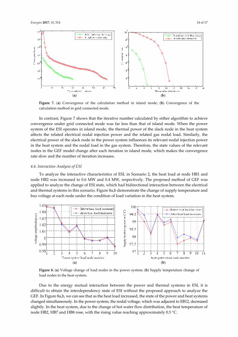
The GEF calculated by the Newton-Raphson, which was initiated randomly, needs 12 times and 64 times to converge to the iterative solution in these two scenarios. However, the proposed method whose state variables were initialized by the homotopy algorithm as per the guidelines given in Section 3.2 only took 5 times and 30 times to converge to the equilibrium point which meets the mismatch tolerance, respectively. The convergence curve of each algorithm in the two scenarios is presented in Figure 7.

Energies 2017, 10, 514 14 of 17

(a) (b)

Figure 7. (a) Convergence of the calculation method in island mode; (b) Convergence of the calculation method in grid connected mode.

In contrast, Figure 7 shows that the iterative number calculated by either algorithm to achieve convergence under grid connected mode was far less than that of island mode. When the power system of the ESI operates in island mode, the thermal power of the slack node in the heat system affects the related electrical nodal injection power and the related gas nodal load. Similarly, the electrical power of the slack node in the power system influences its relevant nodal injection power in the heat system and the nodal load in the gas system. Therefore, the state values of the relevant nodes in the GEF model change after each iteration in island mode, which makes the convergence rate slow and the number of iteration increases.

4.4. Interaction Analysis of ESI

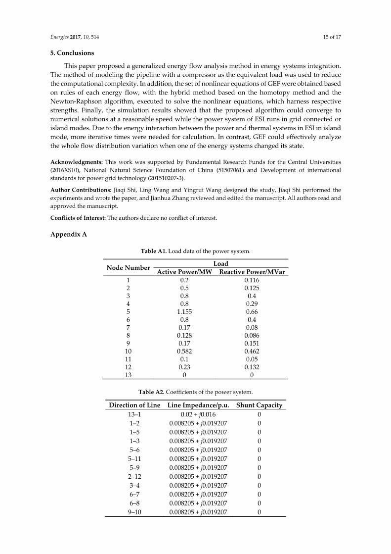
To analyze the interactive characteristics of ESI, in Scenario 2, the heat load at node HB1 and node HB2 was increased to 0.6 MW and 0.4 MW, respectively. The proposed method of GEF was applied to analyze the change of ESI state, which had bidirectional interaction between the electrical and thermal systems in this scenario. Figure 8a,b demonstrate the change of supply temperature and bus voltage at each node under the condition of load variation in the heat system.

volta

ge a

mpl

itude

(p.u

.) o ()C

(a) (b)

Figure 8. (a) Voltage change of load nodes in the power system; (b) Supply temperature change of load nodes in the heat system.

Due to the energy mutual interaction between the power and thermal systems in ESI, it is difficult to obtain the interdependency state of ESI without the proposed approach to analyze the GEF. In Figure 8a,b, we can see that as the heat load increased, the state of the power and heat systems changed simultaneously. In the power system, the nodal voltage, which was adjacent to EB12, decreased slightly. In the heat system, due to the change of hot water flow distribution, the heat temperature of node HB2, HB7 and HB8 rose, with the rising value reaching approximately 0.5 °C.

Energies 2017, 10, 514 15 of 17

5. Conclusions

This paper proposed a generalized energy flow analysis method in energy systems integration. The method of modeling the pipeline with a compressor as the equivalent load was used to reduce the computational complexity. In addition, the set of nonlinear equations of GEF were obtained based on rules of each energy flow, with the hybrid method based on the homotopy method and the Newton-Raphson algorithm, executed to solve the nonlinear equations, which harness respective strengths. Finally, the simulation results showed that the proposed algorithm could converge to numerical solutions at a reasonable speed while the power system of ESI runs in grid connected or island modes. Due to the energy interaction between the power and thermal systems in ESI in island mode, more iterative times were needed for calculation. In contrast, GEF could effectively analyze the whole flow distribution variation when one of the energy systems changed its state.

Acknowledgments: This work was supported by Fundamental Research Funds for the Central Universities (2016XS10), National Natural Science Foundation of China (51507061) and Development of international standards for power grid technology (201510207-3).

Author Contributions: Jiaqi Shi, Ling Wang and Yingrui Wang designed the study, Jiaqi Shi performed the experiments and wrote the paper, and Jianhua Zhang reviewed and edited the manuscript. All authors read and approved the manuscript.

Conflicts of Interest: The authors declare no conflict of interest.

Appendix A

Table A1. Load data of the power system.

Node Number LoadActive Power/MW Reactive Power/MVar

1 0.2 0.1162 0.5 0.1253 0.8 0.44 0.8 0.295 1.155 0.666 0.8 0.47 0.17 0.088 0.128 0.0869 0.17 0.151

10 0.582 0.46211 0.1 0.0512 0.23 0.13213 0 0

Table A2. Coefficients of the power system.

Direction of Line Line Impedance/p.u. Shunt Capacity 13–1 0.02 + j0.016 0 1–2 0.008205 + j0.019207 0 1–5 0.008205 + j0.019207 0 1–3 0.008205 + j0.019207 0 5–6 0.008205 + j0.019207 0 5–11 0.008205 + j0.019207 0 5–9 0.008205 + j0.019207 0 2–12 0.008205 + j0.019207 0 3–4 0.008205 + j0.019207 0 6–7 0.008205 + j0.019207 0 6–8 0.008205 + j0.019207 0 9–10 0.008205 + j0.019207 0

Energies 2017, 10, 514 16 of 17

Table A3. Load data of the heat system.

Node Number Thermal Power/MW Output Temperature/°C 1 0.2 50 2 0.2 50 3 0.2 50 4 0.2 50 5 0.2 50 6 0.2 50 7 0.1 50 8 0.1 50 9 0.3 50 10 0.2 50 11 0.2 50

Table A4. Pipeline coefficients of the heat system.

Direction of Pipeline Length/m Diameter/mm13–1 500 200 1–2 400 200 2–3 600 200 4–3 400 200 12–4 600 200 1–5 200 200

1–6 150 200 2–7 180 200 2–8 150 200 3–9 100 200 3–10 110 200 4–11 90 200

Table A5. Load data of the natural gas system.

Node Number Gas Load/m3h−13 0 4 1100 5 1647.12 6 2000 7 2000

Table A6. Pipeline coefficients of the natural gas system.

Direction of Pipeline Length/m Diameter/mm1–3 500 150 2–6 2500 150 3–4 500 150 3–5 400 150

5–7 600 150 7–6 200 150 3–2 2500 150

Energies 2017, 10, 514 17 of 17

References

1. Rifkin, J. The Third Industrial Revolution; Zhang, T.W., Sun, Y.L., Translators; CITIC Press: Beijing, China, 2012. 2. Shiming, T.; Wenpeng, L.; Dongxia, Z.; Caihao, L.; Yaojie, S. Technical Forms and Key Technologies on

Energy Internet. Proc. CSEE 2015, 35, 3482–3494. 3. Qiuye, S.; Bingyu, W.; Bonan, H.; Dazhong, M. The Optimization Control and Implementation for the

Special Energy Internet. Proc. CSEE 2015, 35, 4571–4580. 4. Geidl, M. Integrated Modeling and Optimization of Multi-Carrier Energy Systems. Ph.D. Thesis, TU Graz,

Graz, Austria, 2007. 5. Mancarella, P. Smart Multi-Energy Grids: Concepts, Benefits and Challenges. In Proceedings of the IEEE

Power and Energy Society General Meeting, San Diego, CA, USA, 22–26 July 2012. 6. Mancarella, P. MES (multi-energy systems): An overview of concepts and evaluation model. Energy 2014,

65, 1–17. 7. Lund, H.; Andersen, A.N.; Østergaard, P.A.; Mathiesen, B.V.; Connolly, D. From electricity smart grids to

smart energy systems—A market operation based approach and understanding. Energy 2012, 42, 96–102. 8. Quelhas, A.; Mccalley, J.D. A Multiperiod Generalized Network Flow Model of the U.S. Integrated Energy

System: Part I—Model Description. IEEE Trans. Power Syst. 2007, 22, 829–836. 9. Martinez-Mares, A.; Fuerte-Esquivel, C.R. A Unified Gas and Power Flow Analysis in Natural Gas and

Electricity Coupled Networks. IEEE Trans. Power Syst. 2012, 27, 2156–2166. 10. Liu, X.; Jenkins, N.; Wu, J.; Bagdanavicius, A. Combined Analysis of Electricity and Heat Networks.

Energy Procedia 2014, 61, 155–159. 11. Zhang, Y. Study on the Methods of Analyzing Combined Gas and Electricity Networks. Master’s Thesis,

China Electric Power Research Institute, Beijing, China, 2005. 12. Chen, S.; Wei, Z.; Sun, G.; Wang, D.; Sun, Y.; Zang, H.; Zhu, Y. Research Center for Renewable Energy

Generation Engineering. Probabilistic Energy Flow Analysis in Integrated Electricity and Natural-gas Energy systems. Proc. CSEE 2015, 35, 6331–6340.

13. Moeini-Aghtaie, M.; Abbaspour, A.; Fotuhi-Firuzabad, M.; Hajipour, E. A Decomposed Solution to Multiple-Energy Carriers Optimal Power Flow. IEEE Trans. Power Syst. 2014, 29, 707–716.

14. Kampouropoulos, K.; Andrade, F.; Sala, E.; Espinosa, A.G.; Romeral, L. Multiobjective Optimization of Multi-Carrier Energy System using a combination of ANFIS and Genetic Algorithms. IEEE Trans. Smart Grid 2016, doi:10.1109/TSG.2016.2609740.

15. Glover, J.D.D.; Sarma, M.S. Power System Analysis and Design; Machinery Industry Press: Beijing, China, 2004. 16. Brown, H.E.; Carter, G.K.; Happ, H.H.; Person, C.E. Power Flow Solution by Impedance Matrix Iterative

Method. IEEE Trans. Power Appar. Syst. 1963, 82, 1–10. 17. Wang, T.; Chiang, H.D. On the Global Convergence of a Class of Homotopy Methods for Nonlinear Circuits

and Systems. IEEE Trans. Circuits Syst. II Express Briefs 2014, 61, 900–904. 18. Carroll, J.J. Natural Gas Hydrates: A Guide for Engineers; Gulf Professional Publishing: Woburn, MA, USA, 2014. 19. Zhao, H. Analysis, modelling and operational optimization of district heating systems. Energy Convers. Manag.

1995, 36, 297–314. 20. De Wolf, D.; Smeers, Y. The Gas Transmission Problem Solved by an Extension of the Simplex Algorithm.

Manag. Sci. 2000, 46, 1454–1465. 21. An, S.; Li, Q.; Gedra, T.W. Natural gas and electricity optimal power flow. In Proceedings of the 2003 IEEE

PES Transmission and Distribution Conference and Exposition, Dallas, TX, USA, 7–12 September 2003; pp. 138–143.

22. Correaposada, C.M.; Sãnchezmartã, N.P. Gas Network Optimization: A comparison of Piecewise Linear Models. 2014. Available online:http://www.optimization-online.org/DB_HTML/2014/10/4580.html (accessed on 10 April 2017).

© 2017 by the authors. Licensee MDPI, Basel, Switzerland. This article is an open access article distributed under the terms and conditions of the Creative Commons Attribution (CC BY) license (http://creativecommons.org/licenses/by/4.0/).