GENERALIZATION OF ROTATIONAL MECHANICS AND …

GENERALIZATION OF ROTATIONAL MECHANICS

AND APPLICATION TO AEROSPACE SYSTEMS

A Dissertation

by

ANDREW JAMES SINCLAIR

Submitted to the Office of Graduate Studies ofTexas A&M University

in partial fulfillment of the requirements for the degree of

DOCTOR OF PHILOSOPHY

May 2005

Major Subject: Aerospace Engineering

CORE Metadata, citation and similar papers at core.ac.uk

Provided by Texas A&M Repository

https://core.ac.uk/display/4269405?utm_source=pdf&utm_medium=banner&utm_campaign=pdf-decoration-v1

GENERALIZATION OF ROTATIONAL MECHANICS

AND APPLICATION TO AEROSPACE SYSTEMS

A Dissertation

by

ANDREW JAMES SINCLAIR

Submitted to Texas A&M Universityin partial fulfillment of the requirements

for the degree of

DOCTOR OF PHILOSOPHY

Approved as to style and content by:

John L. Junkins(Co-Chair of Committee)

John E. Hurtado(Co-Chair of Committee)

Srinivas R. Vadali(Member)

John H. Painter(Member)

Helen L. Reed(Head of Department)

May 2005

Major Subject: Aerospace Engineering

iii

ABSTRACT

Generalization of Rotational Mechanics and Application to Aerospace Systems.

(May 2005)

Andrew James Sinclair, B.S., University of Florida;

M.S., University of Florida

Co–Chairs of Advisory Committee: Dr. John L. JunkinsDr. John E. Hurtado

This dissertation addresses the generalization of rigid-body attitude kinematics,

dynamics, and control to higher dimensions. A new result is developed that demon-

strates the kinematic relationship between the angular velocity in N -dimensions and

the derivative of the principal-rotation parameters. A new minimum-parameter de-

scription of N -dimensional orientation is directly related to the principal-rotation

parameters.

The mapping of arbitrary dynamical systems into N -dimensional rotations and

the merits of new quasi velocities associated with the rotational motion are studied. A

Lagrangian viewpoint is used to investigate the rotational dynamics of N -dimensional

rigid bodies through Poincare’s equations. The N -dimensional, orthogonal angular-

velocity components are considered as quasi velocities, creating the Hamel coefficients.

Introducing a new numerical relative tensor provides a new expression for these co-

efficients. This allows the development of a new vector form of the generalized Euler

rotational equations.

An N -dimensional rigid body is defined as a system whose configuration can

be completely described by an N×N proper orthogonal matrix. This matrix can be

related to an N×N skew-symmetric orientation matrix. These Cayley orientation

variables and the angular-velocity matrix in N -dimensions provide a new connection

iv

between general mechanical-system motion and abstract higher-dimensional rigid-

body rotation. The resulting representation is named the Cayley form.

Several applications of this form are presented, including relating the combined

attitude and orbital motion of a spacecraft to a four-dimensional rotational motion. A

second example involves the attitude motion of a satellite containing three momentum

wheels, which is also related to the rotation of a four-dimensional body.

The control of systems using the Cayley form is also covered. The wealth

of work on three-dimensional attitude control and the ability to apply the Cayley

form motivates the idea of generalizing some of the three-dimensional results to N -

dimensions. Some investigations for extending Lyapunov and optimal control results

to N -dimensional rotations are presented, and the application of these results to

dynamical systems is discussed.

Finally, the nonlinearity of the Cayley form is investigated through computing

the nonlinearity index for an elastic spherical pendulum. It is shown that whereas the

Cayley form is mildly nonlinear, it is much less nonlinear than traditional spherical

coordinates.

v

ACKNOWLEDGMENTS

Special thanks to my advisors Dr. John L. Junkins and Dr. John E. Hurtado.

Their deep insight into dynamics and control and their collegial philosophy has bene-

fited me greatly here at Texas A&M and will continue to do so throughout my career.

I thank my committee members Dr. Rao Vadali and Dr. John Painter for their guid-

ance. I am also grateful to Dr. Daniele Mortari for many educational, constructive,

and entertaining conversations on the subject of generalized rotational mechanics.

Thanks to Lisa Willingham and Karen Knabe for all of their assistance throughout

my degree program.

I wish to thank F. Landis Markley, Robert Bauer, Jackie Schandua, and Michael

Swanzy for their helpful comments and suggestions in the course of preparing this

work. Thanks also to Christian Bruccoleri and Puneet Singla for use of their Mat-

lab code to select initial conditions for computing nonlinearity indices. I gratefully

acknowledge the support of the National Defense Science and Engineering Graduate

Fellowship.

I feel deeply fortunate to have wonderful friends who have made my time in Col-

lege Station a special part of my life: Roshawn Bowers, Eddie Caicedo, Todd Griffith,

Bjoern Kiefer, Luciano Machado, Josh O’Neil, Gary Seidel, Lesley Weitz, and Matt

Wilkins. Finally, I offer my gratitude to my family for their advice, encouragement,

and belief in me.

vi

TABLE OF CONTENTS

CHAPTER Page

I INTRODUCTION . . . . . . . . . . . . . . . . . . . . . . . . . . 1

II KINEMATICS OF N -DIMENSIONAL PRINCIPAL ROTATIONS 5

A. Introduction . . . . . . . . . . . . . . . . . . . . . . . . . . 5

B. Review of N -Dimensional Rotations . . . . . . . . . . . . . 6

1. Rotation Matrix . . . . . . . . . . . . . . . . . . . . . 6

2. Principal Rotation Matrices . . . . . . . . . . . . . . . 9

3. Extended Rodrigues Parameters . . . . . . . . . . . . 10

4. Euler Matrix . . . . . . . . . . . . . . . . . . . . . . . 14

C. Kinematics of Principal Rotations . . . . . . . . . . . . . . 17

D. Optimal Kinematic Maneuvers . . . . . . . . . . . . . . . . 26

E. Conclusion . . . . . . . . . . . . . . . . . . . . . . . . . . . 31

III MINIMUM-PARAMETER REPRESENTATIONS OFN -DI-

MENSIONAL PRINCIPAL ROTATIONS . . . . . . . . . . . . . 33

A. Introduction . . . . . . . . . . . . . . . . . . . . . . . . . . 33

B. Review of N -Dimensional Orientations . . . . . . . . . . . 34

C. Minimal Representations of Principal Rotations . . . . . . 39

1. Numeric Analysis for N = 4 . . . . . . . . . . . . . . . 45

2. Numeric Analysis for N = 5 . . . . . . . . . . . . . . . 49

D. Discussion . . . . . . . . . . . . . . . . . . . . . . . . . . . 55

IV HAMEL COEFFICIENTS FOR THE ROTATIONAL MO-

TION OF AN N -DIMENSIONAL RIGID BODY . . . . . . . . 57

A. Introduction . . . . . . . . . . . . . . . . . . . . . . . . . . 57

B. Review of N -Dimensional Kinematics . . . . . . . . . . . . 59

C. Definition of the Numerical Relative Tensor χjik . . . . . . 62

D. N -Dimensional Hamel Coefficients . . . . . . . . . . . . . . 71

E. Lagrange’s Equations for N -Dimensional Angular Velocities 77

F. The Lax Pair Form Via the Lagrangian Method . . . . . . 79

G. Conclusions . . . . . . . . . . . . . . . . . . . . . . . . . . 82

vii

CHAPTER Page

V CAYLEY KINEMATICS AND THE CAYLEY FORM OF

DYNAMIC EQUATIONS . . . . . . . . . . . . . . . . . . . . . 84

A. Introduction . . . . . . . . . . . . . . . . . . . . . . . . . . 84

B. Cayley Kinematics . . . . . . . . . . . . . . . . . . . . . . 86

C. Tensor Form of Lagrange’s Equations . . . . . . . . . . . . 92

D. Cayley Quasi Velocities and the Cayley Form . . . . . . . 101

E. Planar Motion Example . . . . . . . . . . . . . . . . . . . 104

F. Discussion . . . . . . . . . . . . . . . . . . . . . . . . . . . 109

VI APPLICATION OF THE CAYLEY FORM TO GENERAL

SPACECRAFT MOTION . . . . . . . . . . . . . . . . . . . . . 111

A. Introduction . . . . . . . . . . . . . . . . . . . . . . . . . . 111

B. Cayley Kinematics . . . . . . . . . . . . . . . . . . . . . . 113

C. N -Dimensional Rigid Body Dynamics . . . . . . . . . . . . 114

D. General Spacecraft Motion . . . . . . . . . . . . . . . . . . 116

E. Satellite with Three Momentum Wheels . . . . . . . . . . 124

F. Discussion . . . . . . . . . . . . . . . . . . . . . . . . . . . 127

G. Conclusions . . . . . . . . . . . . . . . . . . . . . . . . . . 130

VII STABILIZATION AND CONTROL OF DYNAMICAL SYS-

TEMS IN THE CAYLEY FORM . . . . . . . . . . . . . . . . . 131

A. Introduction . . . . . . . . . . . . . . . . . . . . . . . . . . 131

B. Definition of Cayley Quasi Velocities . . . . . . . . . . . . 132

C. Linear Rodrigues-Parameter Feedback . . . . . . . . . . . . 135

D. Work/Energy-Rate Expression for N -Dimensional Dynamics 137

E. Feedback Control for N -Dimensional Rotations . . . . . . 140

F. Quasi Velocities for Linear Feedback . . . . . . . . . . . . 148

G. Optimality Results for Regulation Terms . . . . . . . . . . 151

H. Stabilization Using Velocity Feedback . . . . . . . . . . . . 154

I. Conclusion . . . . . . . . . . . . . . . . . . . . . . . . . . . 158

VIII NONLINEARITY INDEX OF THE CAYLEY FORM . . . . . . 160

A. Introduction . . . . . . . . . . . . . . . . . . . . . . . . . . 160

B. Nonlinearity Index . . . . . . . . . . . . . . . . . . . . . . 161

C. Elastic Spherical Pendulum . . . . . . . . . . . . . . . . . 163

D. Numerical Results . . . . . . . . . . . . . . . . . . . . . . . 167

E. Discussion . . . . . . . . . . . . . . . . . . . . . . . . . . . 172

viii

CHAPTER Page

IX SUMMARY . . . . . . . . . . . . . . . . . . . . . . . . . . . . . 174

REFERENCES . . . . . . . . . . . . . . . . . . . . . . . . . . . . . . . . . . . 176

APPENDIX A . . . . . . . . . . . . . . . . . . . . . . . . . . . . . . . . . . . 182

APPENDIX B . . . . . . . . . . . . . . . . . . . . . . . . . . . . . . . . . . . 183

APPENDIX C . . . . . . . . . . . . . . . . . . . . . . . . . . . . . . . . . . . 185

VITA . . . . . . . . . . . . . . . . . . . . . . . . . . . . . . . . . . . . . . . . 190

ix

LIST OF TABLES

TABLE Page

I EXAMPLE OF ORTHOGONAL PLANES FOR N = 6 . . . . . . . 61

II CORRESPONDING VALUES OF i, j, AND k . . . . . . . . . . . . 64

III SUMMARY OF PROPERTIES RELATED TO χjik . . . . . . . . . . 71

IV THE CAYLEY FORM OF DYNAMIC EQUATIONS . . . . . . . . . 103

V ELASTIC SPHERICAL PENDULUM REPRESENTATIONS . . . . 165

VI NUMERICAL RESULTS FOR NONLINEARITY . . . . . . . . . . . 169

x

LIST OF FIGURES

FIGURE Page

1 Coordinatization of the principal plane by p(1) and p(2) frames,

which are related by a flipping about the axis a. . . . . . . . . . . . 44

2 Relationships between four of the eight solutions for N = 4: f -

flip, s - swap, fs - flip and swap. . . . . . . . . . . . . . . . . . . . . . 50

3 Relationships between four of the sixteen solutions for N = 5: fr

- flip-rotate, rf - rotate-flip, ff - flip-flip. . . . . . . . . . . . . . . . . . 54

4 Planar rigid body. . . . . . . . . . . . . . . . . . . . . . . . . . . . . 106

5 Generalized coordinates. . . . . . . . . . . . . . . . . . . . . . . . . . 107

6 Generalized velocities. . . . . . . . . . . . . . . . . . . . . . . . . . . 108

7 Cayley quasi velocities. . . . . . . . . . . . . . . . . . . . . . . . . . . 108

8 Example planar motion. . . . . . . . . . . . . . . . . . . . . . . . . . 109

9 Attitude and orbital motion variables. . . . . . . . . . . . . . . . . . 123

10 Attitude and orbital motion Cayley quasi velocities. . . . . . . . . . . 123

11 Satellite system motion variables. . . . . . . . . . . . . . . . . . . . . 128

12 Satellite system Cayley quasi velocities. . . . . . . . . . . . . . . . . 128

13 Possible mappings between three equivalent systems. . . . . . . . . . 129

14 Control vector magnitude time history. . . . . . . . . . . . . . . . . . 157

15 Kinetic energy time history. . . . . . . . . . . . . . . . . . . . . . . . 158

16 Elastic spherical pendulum. . . . . . . . . . . . . . . . . . . . . . . . 163

17 Nominal trajectory in Cartesian coordinates. . . . . . . . . . . . . . . 168

xi

FIGURE Page

18 Nominal trajectory in spherical coordinates. . . . . . . . . . . . . . . 169

19 Nominal trajectory for Cayley quasi velocities. . . . . . . . . . . . . . 170

20 Nonlinearity index for spherical coordinates. . . . . . . . . . . . . . . 170

21 Nonlinearity index for Cayley form. . . . . . . . . . . . . . . . . . . . 171

22 Linearization error in motion constants for spherical coordinates. . . 171

23 Linearization error in motion constants for Cayley form. . . . . . . . 172

1

CHAPTER I

INTRODUCTION

This dissertation deals with the generalization of rotational mechanics to describe

N -dimensional rotations. The field of rotational mechanics has been developed to

describe the orientation, kinematics, dynamics, and control of rigid bodies and has

been key in the development of aerospace vehicles. The first elements of this theory

were laid down over 250 years ago, and the field has been the subject of continued

attention over the past fifty years with the development of spacecraft technology.

Although this field has been developed to describe physical, three-dimensional bodies,

many of the concepts that have been developed can be extended to mathematically

describe higher-dimensional bodies. The first half of this dissertation reviews the

kinematics and dynamics ofN -dimensional rotations, as well as presenting several new

ideas. The second half of the dissertation presents and investigates the implications

of a new idea to use N -dimensional rotational concepts to describe the motion of real,

physical systems. An example of this approach is applied to spacecraft orbital and

attitude dynamics, and a new approach for feedback control design is presented.

Although not as old as the study of three-dimensional rotations, the field of N -

dimensional rotations has developed for more than 150 years. Much of Chapter II

of this dissertation deals with reviewing generalizations of three-dimensional attitude

descriptions to N -dimensional orientation. Fundamental to establishing a geomet-

ric interpretation of N -dimensional rotations is the extension of Euler’s theorem to

higher dimensions. Although there is only one principal plane for any rotation in

three-dimensions, an additional principal plane is added with every increase in dimen-

The journal model is IEEE Transactions on Automatic Control.

2

sion by two dimensions. Several of the attitude representations for three-dimensional

rotations can be directly extended to N -dimensional rotations, and like many of the

concepts in this dissertation, three-dimensional representations are actually just a

special case of the general form. In particular, attitude representations related to

the Cayley transform and higher-order Cayley transforms have direct N -dimensional

generalizations. These generalizations carry over relationships to the principal rota-

tions and singularity conditions, for which the parameters are undefined, similar to

the three-dimensional special cases. Chapters II and III also present several new ideas

for describing N -dimensional orientations and their evolution.

In Chapters IV and V the focus shifts from kinematics to dynamics. Again, the

dynamics of N -dimensional rotations have been studied for over 125 years. Equations

of motion have been developed for these rotations by extending the concept of angular-

momentum conservation under the assumption of a symmetric, unforced system. Here

though, two new derivations of these equations are presented. The new derivations

link N -dimensional rotational mechanics to Lagrangian dynamics for the first time,

which is made possible by the introduction of a new numerical relative tensor. Some

important features of the new derivations are that they provide a vector form of the

equations of motion and, by removing the assumptions of symmetry and unforced

motion, they allow for applied forces and coordinate dependence.

Considering applied forces and coordinate dependence is necessary to allow the

application of these rotational equations to a broader class of problems, which is

the subject of the second half of the dissertation. The new idea of describing the

motion of real, physical systems using the N -dimensional kinematic and dynamic

equations is presented. This idea associates the rotation of an N -dimensional rigid

body with the motion of any given system, or in other words, views the motion as

an N -dimensional rotation. This concept is called the Cayley form. Specifically, the

3

generalized coordinates of the system are treated as orientation variables of an N -

dimensional rigid body, and the Cayley form defines a set of quasi velocities for the

system that are equal to the angular velocity of the N -dimensional body. In Chapter

VI two examples are presented treating the dynamics of physical systems using the

Cayley form, including treating the combined orbital and attitude dynamics of a

spacecraft as pure rotation of a four-dimensional body.

Chapter VII presents some results for designing feedback controllers using the

Cayley form. The idea behind this approach is to generalize spacecraft attitude

controllers to N -dimensional rotations and then use the Cayley form to apply these

to general systems. The motivation for this is the possibility to leverage the wealth of

work that has been produced over the past fifty years for spacecraft attitude control

in application to broader classes of systems. An example is shown, though, that

spacecraft attitude control can be based on the special properties of three-dimensional

rotations that do not hold for general N -dimensional kinematics. The rotational

dynamics, however, do not appear as sensitive to generalization to N -dimensions, and

an example is presented taking advantage of this in designing a stabilizing controller

for a three-link manipulator system.

Finally, some issues dealing with the complexity or nonlinearity of the Cayley

form are addressed in Chapter VIII. Several measures of nonlinearity are computed

for an elastic spherical pendulum. It is shown that whereas applying the Cayley form

to an originally linear system produces a mildly nonlinear system, the Cayley form

can also be much less nonlinear than traditional alternative representations.

Index notation is used extensively throughout the dissertation. The elements of

a matrix or tensor, A, are expressed as Aij and the elements of a vector, a, as ai.

The Einstein summation convention is that if any index is repeated twice within a

term, then the term represents the summation for every possible value of the index.

4

An index must not be repeated more than twice in a term. Indices that appear only

once in each term of an equation are free indices, and the equation is valid for each

possible value of the index. The Kronecker delta, δij, is equal to unity if i = j and is

equal to zero otherwise.

5

CHAPTER II

KINEMATICS OF N -DIMENSIONAL PRINCIPAL ROTATIONS

A. Introduction

An important description of three-dimensional rotations is provided by Euler’s the-

orem that describes any general orientation in terms of a single principal rotation.

The principal rotation concept also extends to N -dimensional rotations [1], however,

for higher-dimensional spaces a general orientation requires N/2 principal rotations

for even N and (N − 1)/2 principal rotations for odd N . In general the number of

required rotations can be expressed as L = N/2. These rotations take place on

completely orthogonal planes, called the principal planes. For even dimensions these

planes completely occupy the space. For odd dimensions, however, one axis is left

out of the rotational motion and is referred to as a principal axis.

In addition to Euler’s theorem, key representations of an orientation in N -

dimensional space are the proper-orthogonal rotation matrix, the extended Rodrigues

parameters (ERPs), and the Euler Matrix. For any given orientation, the principal

rotations (planes and angles) can be computed from a variety of methods. These

methods are different decompositions of the representations mentioned above. Some

of the methods are a spectral decomposition described by Mortari [2], a principal

rotation matrix decomposition also developed by Mortari [2], a canonical form de-

scribed by Bauer [3], and a minimum-parameter canonical form developed by Sinclair

and Hurtado [4]. Of course each of these representations is related, and the above

references largely deal with the interconnections between the different decompositions.

As will be described, the canonical form decomposes the various representation

matrices into a block-diagonal form with a 2× 2 block associated with each principal

6

plane and a 1 × 1 block associated with the principal axis if it exists. In illustrating

these blocks, the notation [A] (a : b) will be used to refer to the block on the diagonal

of the matrix A from the ath row and column to the bth row and column. Addition-

ally, in the following sections the spectral decomposition and canonical form of the

various rotation variables will be illustrated for odd N . The corresponding forms for

even N can be constructed by simply deleting the Nth row and column which will

be associated with the principal axis.

B. Review of N -Dimensional Rotations

Much of the description of N -dimensional orientations in this section was given by

Mortari [2] and Bauer [3]. The current work attempts to follow their notation and

conventions as closely as possible with one exception. In discussing a rotated frame

both of the above authors define representations of the rotation as the mapping from

the rotated frame back to a reference frame. Here the convention will be to give

the mapping from the reference frame to the rotated frame. Therefore, many of the

definitions given below correspond to the transpose of the proper rotation matrices

given by Mortari and Bauer.

1. Rotation Matrix

The transformation of an N -dimensional vector by a proper orthogonal matrix, C,

describes a rotation in N -dimensional space. The following equation describes the

transformation from a column matrix parameterizing a vector in a reference coordi-

nate system, the n frame, to a column matrix parameterizing the vector in a rotated

coordinate system, the b frame.

[r]b = [C] [r]n (2.1)

7

Alternatively, Eq. (2.1) can be viewed as simply an orthogonal projection of the com-

ponents of an arbitrary vector. This matrix C is called a rotation matrix and is

the most fundamental representation of N -dimensional rotations. Two complemen-

tary representations of the rotation matrix that will be considered are the spectral

decomposition and the canonical form.

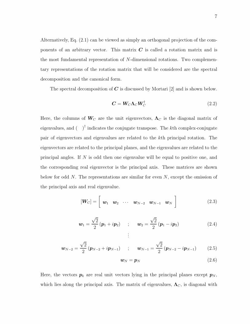
The spectral decomposition of C is discussed by Mortari [2] and is shown below.

C = WCΛCW †C (2.2)

Here, the columns of WC are the unit eigenvectors, ΛC is the diagonal matrix of

eigenvalues, and ( )†

indicates the conjugate transpose. The kth complex-conjugate

pair of eigenvectors and eigenvalues are related to the kth principal rotation. The

eigenvectors are related to the principal planes, and the eigenvalues are related to the

principal angles. If N is odd then one eigenvalue will be equal to positive one, and

the corresponding real eigenvector is the principal axis. These matrices are shown

below for odd N . The representations are similar for even N , except the omission of

the principal axis and real eigenvalue.

[WC ] =

[w1 w2 · · · wN−2 wN−1 wN

](2.3)

w1 =

√2

2(p1 + ip2) ; w2 =

√2

2(p1 − ip2) (2.4)

...

wN−2 =

√2

2(pN−2 + ipN−1) ; wN−1 =

√2

2(pN−2 − ipN−1) (2.5)

wN = pN (2.6)

Here, the vectors pk are real unit vectors lying in the principal planes except pN ,

which lies along the principal axis. The matrix of eigenvalues, ΛC , is diagonal with

8

values λ(C)k .

λ(C)1 = cos (φ1 + 2πn1) + i sin (φ1 + 2πn1) (2.7)

λ(C)2 = cos (φ1 + 2πn1) − i sin (φ1 + 2πn1) (2.8)

...

λ(C)N−2 = cos (φL + 2πnL) + i sin (φL + 2πnL) (2.9)

λ(C)N−1 = cos (φL + 2πnL) − i sin (φL + 2πnL) (2.10)

λ(C)N = + 1 (2.11)

Here, each angle −π ≤ φk ≤ π is the value of rotation in the kth principal plane, and

the values nk can be any integer. It is important to note that the matrices WC and

ΛC are not unique. This is because of the ambiguity in selecting the vectors pk (they

can lie anywhere in the principal plane) as well as the existence of multiple choices

for ordering the eigenvectors and eigenvalues within WC and ΛC (i.e., labeling the

principal planes one through L).

The canonical representation of C is related to the spectral decomposition [3].

C = P T C ′P ; C ′ = PCP T (2.12)

Here, P is a proper orthogonal matrix, and C ′ is a block-diagonal proper orthogonal

matrix. The rows of P are the coordinatization of the principal coordinate vectors

in the b frame.

[P ]T =

[[p1]b [p2]b . . . [pN ]b

](2.13)

9

The matrix C ′ is related to the principal angles. The kth block on the diagonal of

C ′ has the following form.

[C ′] (2k − 1 : 2k) =

⎡⎢⎣ cos (φk + 2πnk) sin (φk + 2πnk)

− sin (φk + 2πnk) cos (φk + 2πnk)

⎤⎥⎦ (2.14)

For odd N the (N,N) element of C ′ forms a 1 × 1 block and is equal to +1.

The matrix P is itself an N -dimensional rotation matrix that describes the trans-

formation from the rotated frame to a third frame, the principal frame. This coor-

dinate system has coordinate vectors p1,p2, . . . ,pN which are aligned with the

principal planes of the rotation described by C: (p1,p2), (p3,p4), etc. Note that

consistent with his convention mentioned earlier, Bauer defines P as the transpose of

the definition given here; thus it is the mapping from the principal to rotated frame.

2. Principal Rotation Matrices

Another representation of N -dimensional orientation that is closely related to the

principal planes and angles involves the principal rotation matrices. These are L

proper orthogonal matrices, each describing one of the principal rotations that com-

pose a general orientation [2].

C = R1R2 . . .RL = R1 + R2 + . . . + RL − (L− 1) I (2.15)

The remarkable fact that C can be expressed as either a product or sum of the prin-

cipal rotation matrices is due to the complete orthogonality of the planes in which

the rotations occur. The elegant decomposition of Eq. (2.15) was discovered by Mor-

tari [2]. Note that Mortari uses the convention that a rotation is an orientation that

can be described by only one nonzero principal rotation (hence, the terms rotation

10

and orientation are equivalent only for N = 2 or 3) and simply refers to the R

matrices as rotation matrices; this terminology is not entirely adopted here.

Mortari gives the relationship between the principal rotation matrices and the

principal planes and angles [2]. These expressions are written in terms of the rows of

P arranged in N × 2 matrices and the 2 × 2 symplectic matrix.

[Pk] =

[[p2k−1]b [p2k]b

]; [J ] =

⎡⎢⎣ 0 1

−1 0

⎤⎥⎦ (2.16)

The principal rotation matrices are given as follows [2].

Rk (Pk, φk) = I + (cos φk − 1)PkPTk + PkJP T

k sinφk (2.17)

Note that this expression is identical to the one given by Mortari in spite of the fact

that the symplectic matrix defined in Eqs. (2.16) is the transpose of the matrix used

by Mortari. The implication of this change in J is that, whereas the principal rotation

matrix Rk (Pk, φk) defined by Mortari describes a rotation of −φk, the current defi-

nitions describe a rotation of positive φk. Conversely the rotation matrix as defined

by Mortari can be seen as the transformation matrix from a frame that is rotated by

φk back to some reference frame, whereas the current definition is the rotation from

the reference to the rotated frame.

3. Extended Rodrigues Parameters

The rotation matrix has N2 elements and is subject to N2 −M orthogonality con-

straints, where the minimum number of parameters necessary to represent an N -

dimensional rotation is M = 12N(N − 1). A commonly used minimum parameter

representation is the extended Rodrigues parameters (ERPs) [5, 6]. These parame-

ters are defined by the Cayley transform, which relates proper orthogonal and skew-

11

symmetric matrices [7]. Cayley discovered the forward relationship while investigating

some properties of “left systems” [8].

Forward: C = (I −Q) (I + Q)−1 = (I + Q)−1 (I − Q) (2.18)

Inverse: Q = (I −C) (I + C)−1 = (I + C)−1 (I −C) (2.19)

Here, Q is an N × N skew-symmetric matrix, and I is the identity matrix. The

M distinct elements of the matrix Q comprise the ERPs. Although the forward

transformation is valid for all Q = −QT , the inverse transformation is singular for

the “180 rotations” where det (I + C) vanishes.

The eigenvalues and eigenvectors of Q can be found by substituting the spectral

decomposition of C into the Cayley transform, Eq. (2.19).

Q = (I + C)−1 (I − C) =(I + WCΛCW †

C

)−1 (I − WCΛCW †

C

)(2.20)

=[WC (I + ΛC)W †

C

]−1 [WC (I − ΛC)W †

C

]= WC (I + ΛC)−1 (I − ΛC)W †

C

Therefore, the eigenvectors of Q can be set equal to the eigenvectors of C: WQ = WC .

The following is concluded for the eigenvalues of Q.

ΛQ = (I + ΛC)−1 (I −ΛC) (2.21)

Because each of the above matrices are diagonal, the individual eigenvalues are related

as follows.

λ(Q)k =

1 − λ(C)k

1 + λ(C)k

(2.22)

12

Comparing this result with Eqs. (2.7) to (2.11) relates the eigenvalues of Q to the

principal angles.

λ(Q)1 = −i tan

(φ1 + 2πn1

2

); λ

(Q)2 = i tan

(φ1 + 2πn1

2

)(2.23)

...

λ(Q)N−2 = −i tan

(φL + 2πnL

2

); λ

(Q)N−1 = i tan

(φL + 2πnL

2

)(2.24)

λ(Q)N = 0 (2.25)

The canonical form of Q relates the ERPs to the canonical form of C. The

canonical representation of a skew-symmetric matrix decomposes the matrix into a

proper orthogonal matrix and a block-diagonal skew-symmetric matrix [3, 9]. These

matrices can be found by substituting the canonical form of C into the Cayley trans-

form, Eq. (2.19).

Q = (I + C)−1 (I − C) =(I + P TC ′P

)−1 (I −P T C ′P

)=[P T (I + C ′) P

]−1 [P T (I − C ′) P

]= P T (I + C ′)−1

(I − C ′) P (2.26)

The Cayley transform of C ′ is a block-diagonal, skew-symmetric matrix and is defined

as Q′.

Q′ = (I + C ′)−1(I − C ′) ; C ′ = (I + Q′)−1

(I −Q′) (2.27)

Therefore, the same proper orthogonal matrix P transforms C and Q to canonical

form.

Q = P T Q′P ; Q′ = PQP T (2.28)

The elements of this new skew-symmetric matrix Q′ are referred to as the canonical

ERPs. The similarity transformation enforces that Q and Q′ share the same eigen-

values and their eigenvectors are related through P . By convention the following

13

form is chosen for Q′ for odd N .

[Q′] =

⎡⎢⎢⎢⎢⎢⎢⎢⎢⎢⎢⎢⎢⎢⎢⎣

0 Q′12 · · · 0 0 0

−Q′12 0 · · · 0 0 0

......

. . ....

......

0 0 · · · 0 Q′N−1,N 0

0 0 · · · −Q′N−1,N 0 0

0 0 · · · 0 0 0

⎤⎥⎥⎥⎥⎥⎥⎥⎥⎥⎥⎥⎥⎥⎥⎦(2.29)

In the canonical representation of Q, the matrix Q′ is related to the principal

angles, and P is related to the principal planes. The kth block on the diagonal of Q′

is related to the angle of the kth principal rotation as follows.

Q′2k−1,2k = − tan

(φk + 2πnk

2

)(2.30)

The sign convention above is chosen to be consistent with the canonical form of C in

Eq. (2.14).

The canonical form of Q is also directly related to the principal rotation matrices,

Rk. These rotation matrices are simply the canonical transformation of the Cayley

transform of each block on the diagonal of Q′. The individual blocks of Q′ can be

separated as follows.

Q′ = Q′1 + Q′

2 + . . . + Q′L (2.31)

14

Here, each Q′k contains only one of the blocks on the diagonal of Q′. For example, in

a five-dimensional rotation Q′ will consist of Q′1 and Q′

2.

[Q′1] =

⎡⎢⎢⎢⎢⎢⎢⎢⎢⎢⎢⎣

0 Q′12 0 0 0

−Q′12 0 0 0 0

0 0 0 0 0

0 0 0 0 0

0 0 0 0 0

⎤⎥⎥⎥⎥⎥⎥⎥⎥⎥⎥⎦; [Q′

2] =

⎡⎢⎢⎢⎢⎢⎢⎢⎢⎢⎢⎣

0 0 0 0 0

0 0 0 0 0

0 0 0 Q′34 0

0 0 −Q′34 0 0

0 0 0 0 0

⎤⎥⎥⎥⎥⎥⎥⎥⎥⎥⎥⎦(2.32)

Returning to Eq. (2.27), the two terms involving Q′ can be expanded using the

matrices Q′k.

(I + Q′)−1= (I + Q′

1)−1. . . (I + Q′

L)−1

(2.33)

(I − Q′) = (I − Q′1) . . . (I − Q′

L) (2.34)

These expansions can be used to rewrite the canonical form of C.

C = P T (I + Q′1)

−1. . . (I + Q′

L)−1

(I − Q′1) . . . (I − Q′

L)P (2.35)

Because of the special form of the Q′k matrices, this product can be rearranged as

follows.

C = P T (I + Q′1)

−1(I − Q′

1) . . . (I + Q′L)

−1(I − Q′

L) P (2.36)

Comparing this result with Eq. (2.15), one can choose the principal rotation matrices

as shown below.

Rk = P T (I + Q′k)

−1(I − Q′

k)P (2.37)

4. Euler Matrix

A final representation of N -dimensional rotations that will be useful for the current

purposes is the Euler matrix. Whereas this matrix has been used tangentially in

15

previous works [2, 10], it will be developed more fully here. The Euler matrix is a

skew-symmetric matrix, E, that can be related to the rotation matrix using properties

of the matrix exponential and determinant [11].

exp (E) (exp (E))T

= exp(E) exp(ET)

= exp(E + ET

)= exp (0) = I (2.38)

det (exp (E)) = exp (Tr (E)) = exp (0) = +1 (2.39)

Because exp (E) is proper orthogonal, the following relationship to the rotation matrix

can be considered the definition of the Euler matrix.

C = exp (E) (2.40)

Based on this definition it is possible to relate the Euler matrix to the principal

rotations and solve for E. Although it is tempting to simply write E = ln (C), it

will be shown that this mapping is not unique because infinitely many solutions for

E correspond to any particular orientation. Additionally, the matrix logarithm can

suffer from limited range of convergence [11].

To relate the Euler matrix to the principal rotations, the spectral decomposition

of E will be considered.

E = WEΛEW †E (2.41)

Here, WE is a matrix of the unit eigenvectors of E. This matrix is not unique,

however, because of the ambiguity in the complex-conjugate pairs of eigenvectors as

well as the existence of multiple choices for ordering the eigenvectors within WE . The

matrix exponential of Eq. (2.41) is shown below.

exp (E) = WE exp (ΛE)W †E (2.42)

16

Comparing this expression with the definition of the Euler matrix relates the eigen-

values of C and E. By properly choosing the eigenvector ordering within WC and

WE , the following matrix equality can be set.

ΛC = exp (ΛE) (2.43)

Of course, because the eigenvalue matrices are diagonal the matrix exponential sim-

plifies to the exponential of each eigenvalue element. Comparing this result with

Eqs. (2.7) to (2.11) gives the eigenvalues of E.

λ(E)1 = i (φ1 + 2πn1) ; λ

(E)2 = −i (φ1 + 2πn1) (2.44)

...

λ(E)N−2 = i (φL + 2πnL) ; λ

(E)N−1 = −i (φL + 2πnL) (2.45)

λ(E)N = 0 (2.46)

Next, the canonical form of the Euler matrix can be considered which relates E

to a canonical transformation matrix and a block-diagonal skew-symmetric matrix

E′.

E = P TE′P (2.47)

Taking the exponential of Eq. (2.47) and comparing to Eq. (2.12) demonstrates that

the same canonical transformation matrix P applied to C and Q can also be applied

to E. The matrix C ′ is the matrix exponential of E′. The matrices E and E′

share the same eigenvalues. Because E′ is block-diagonal, however, its kth pair of

eigenvalues are simply λ(E′)2k−1 = iE ′

2k−1,2k and λ(E′)2k = −iE ′

2k−1,2k. Comparing this with

17

Eqs. (2.44) to (2.46) gives the elements of E′.

[E′] =

⎡⎢⎢⎢⎢⎢⎢⎢⎢⎢⎢⎢⎢⎢⎢⎣

0 φ1 + 2πn1 · · · 0 0 0

−φ1 − 2πn1 0 · · · 0 0 0

......

. . ....

......

0 0 · · · 0 φL + 2πnL 0

0 0 · · · −φL − 2πnL 0 0

0 0 · · · 0 0 0

⎤⎥⎥⎥⎥⎥⎥⎥⎥⎥⎥⎥⎥⎥⎥⎦(2.48)

Again, the sign convention above is chosen to be consistent with C ′ in Eq. (2.14).

Because of the ambiguity in nk, infinitely many values of E′ and E exist which

correspond to any particular C.

C. Kinematics of Principal Rotations

In the previous section several methods to describe N -dimensional rotations in terms

of the principal planes and angles were reviewed. In this section these results will

be extended to relate the N -dimensional angular velocity and the derivatives of the

principal planes and angles. This will result in kinematic differential equations for P

and φk.

Traditionally the kinematic evolution of N -dimensional rotations have not been

related to the principal rotations. Instead, equations for the derivatives of C or Q

are used directly. The first is provided by Poisson’s equation.

C = −ΩC (2.49)

Here, Ω is the N -dimensional skew-symmetric angular-velocity matrix. This equation

and the Cayley transform can be used to derive the Cayley-transform kinematic

relationships, which connect the derivative of Q to the angular-velocity matrix; these

18

results were first developed by Junkins and Kim [12].

Ω = 2 (I + Q)−1 Q (I − Q)−1 ; Q =1

2(I + Q) Ω (I − Q) (2.50)

Whereas both Poisson’s equation and the Cayley-transform kinematic relation-

ships hold for any value of N , for three-dimensional rotations there also exists rela-

tionships between the angular velocity and the derivatives of the principal angle, φ,

and principal axis, a. These can be developed by writing the rotation matrix C as

a function of φ and a and then taking the derivative. These expressions are then

substituted into Eq. (2.49), which is solved for Ω [13]. In fact, a similar procedure

can be used to relate the N -dimensional angular velocity to the derivatives of P and

φk.

The kinematic equations for the principal planes and angles of a four-dimensional

rotation will be developed here. For four dimensions the canonical transformation

matrix has the following form.

[P ]T

=

[P1 P2

]=

[[p1]b [p2]b [p3]b [p4]b

](2.51)

Again, p1 and p2 are orthogonal vectors lying in the first principal plane, whereas

p3 and p4 are orthogonal vectors lying in the second principal plane, completely

orthogonal to the first. To develop the kinematic equations, the rotation matrix is

written in terms of the two principal rotation matrices.

C = R1 + R2 − I (2.52)

= I + (cosφ1 − 1)P1PT1 + sinφ1P1JP T

1 + (cos φ2 − 1) P2PT2 + sinφ2P2JP T

2

CT = I + (cosφ1 − 1)P1PT1 − sin φ1P1JP T

1 + (cosφ2 − 1) P2PT2 − sinφ2P2JP T

2

(2.53)

19

C = − φ1 sin φ1P1PT1 + (cos φ1 − 1)

(P1P

T1 + P1P

T1

)+ φ1 cos φ1P1JP T

1

+ sinφ1

(P1JP T

1 + P1JP T1

)− φ2 sinφ2P2P

T2 + (cosφ2 − 1)

(P2P

T2 + P2P

T2

)+ φ2 cosφ2P2JP T

2 + sinφ2

(P2JP T

2 + P2JP T2

)(2.54)

The product of Eqs. (2.53) and (2.54) is evaluated to find Ω = −CCT . This expansion

is simplified using the following identities.

pTi pj =

⎧⎪⎨⎪⎩ 1 for i = j

0 for i = j(2.55)

This implies the following.

P T1 P1 = P T

2 P2 = I ; P T1 P2 = 0 (2.56)

Additionally the square of the symplectic matrix is given by JJ = −I. Using these

identities, the terms of the product are collected into terms containing the derivatives

φ1 and φ2 and terms containing the derivatives P1 and P2.

20

Ω = −φ1P1JP T1 − φ2P2JP T

2 +[(1 − cos φ1)

(P1P

T1 − P1P

T1

)− sinφ1

(P1JP T

1 + P1JP T1

)− (1 − cosφ1) (1 − cosφ2)P1P

T1 P2P

T2

− (1 − cos φ1) sin φ2P1PT1 P2JP T

2 + sinφ1 (1 − cos φ2)P1JP T1 P2P

T2

+ sinφ1 sinφ2P1JP T1 P2JP T

2 − (1 − cos φ1)2 P1P

T1 P1P

T1

+sin φ1 (1 − cosφ1)(P1JP T

1 P1PT1 − P1P

T1 P1JP T

1

)+ sin2 φ1P1JP T

1 P1JP T1

]+[(1 − cosφ2)

(P2P

T2 − P2P

T2

)− sinφ2

(P2JP T

2 + P2JP T2

)− (1 − cos φ1) (1 − cosφ2)P2P

T2 P1P

T1 + sinφ1 (1 − cos φ2)P2P

T2 P1JP T

1

+ (1 − cos φ1) sinφ2P2JP T2 P1P

T1 + sin φ1 sin φ2P2JP T

2 P1JP T1

− (1 − cos φ2)2 P2P

T2 P2P

T2 + sinφ2 (1 − cos φ2)

(P2JP T

2 P2PT2 − P2P

T2 P2JP T

2

)+sin2 φ2P2JP T

2 P2JP T2

](2.57)

Further simplifications can be made by investigating the derivatives of P1 and P2.

These are found by using the orthogonality of P .

PP T =

⎡⎢⎣ P T1

P T2

⎤⎥⎦[ P1 P2

]=

⎡⎢⎣ P T1 P1 P T

1 P2

P T2 P1 P T

2 P2

⎤⎥⎦ (2.58)

Because P must obey Poisson’s equation the above product must be skew-symmetric

(and in fact is related to the angular-velocity matrix of the principal frame relative

to the rotated frame). This implies the following.

P T1 P1 = −P T

1 P1 ; P T2 P2 = −P T

2 P2 ; P T1 P2 = −

(P T

2 P1

)T

= −P T1 P2 (2.59)

Finally, the terms involving J can be collected using the following identities.

P T1 P1 =

⎡⎢⎣ pT1

pT2

⎤⎥⎦[ p1 p2

]=

⎡⎢⎣ pT1 p1 pT

1 p2

pT2 p1 pT

2 p2

⎤⎥⎦ =

⎡⎢⎣ 0 pT1 p2

−pT1 p2 0

⎤⎥⎦ (2.60)

21

JP T1 P1 =

⎡⎢⎣ 0 1

−1 0

⎤⎥⎦⎡⎢⎣ 0 pT

1 p2

−pT1 p2 0

⎤⎥⎦ =

⎡⎢⎣ −pT1 p2 0

0 −pT1 p2

⎤⎥⎦ (2.61)

P T1 P1J =

⎡⎢⎣ 0 pT1 p2

−pT1 p2 0

⎤⎥⎦⎡⎢⎣ 0 1

−1 0

⎤⎥⎦ =

⎡⎢⎣ −pT1 p2 0

0 −pT1 p2

⎤⎥⎦ = JP T1 P1 (2.62)

JP T1 P1J =

⎡⎢⎣ 0 1

−1 0

⎤⎥⎦⎡⎢⎣ −pT

1 p2 0

0 −pT1 p2

⎤⎥⎦ =

⎡⎢⎣ 0 −pT1 p2

pT1 p2 0

⎤⎥⎦ = −P T1 P1

(2.63)

Of course, the identities analogous to those shown for P1 and P1 in Eqs. (2.60) through

(2.63) also hold for P2 and P2. These lead to the following expression for CCT .

Ω = −φ1P1JP T1 − φ2P2JP T

2 +[(1 − cosφ1)

(P1P

T1 − P1P

T1

)− sinφ1

(P1JP T

1 + P1JP T1

)− (1 − cos φ1) (1 − cosφ2)P1P

T1 P2P

T2

− (1 − cos φ1) sinφ2P1PT1 P2JP T

2 + sin φ1 (1 − cosφ2)P1JP T1 P2P

T2

+sin φ1 sinφ2P1JP T1 P2JP T

2 − 2 (1 − cosφ1)P1PT1 P1P

T1

]+[(1 − cos φ2)

(P2P

T2 − P2P

T2

)− sinφ2

(P2JP T

2 + P2JP T2

)− (1 − cos φ1) (1 − cos φ2)P2P

T2 P1P

T1 − sinφ1 (1 − cos φ2)P2P

T2 P1JP T

1

+ (1 − cos φ1) sinφ2P2JP T2 P1P

T1 + sinφ1 sinφ2P2JP T

2 P1JP T1

−2 (1 − cos φ2)P2PT2 P2P

T2

](2.64)

This expression can be simplified by mapping it to the principal coordinate frame.

This is done by applying the following similarity transformation.

[PΩP T

]=

⎡⎢⎣ P T1

P T2

⎤⎥⎦ [Ω]

[P1 P2

]=

⎡⎢⎣ P T1 ΩP1 P T

1 ΩP2

P T2 ΩP1 P T

2 ΩP2

⎤⎥⎦ (2.65)

22

Whereas the similarity transformation P mapped the skew-symmetric matrices Q

and E into a canonical form, here Ω is a different matrix and will have a different

canonical transformation. Equation (2.65) is skew-symmetric but not block-diagonal

in general. The individual terms of Eq. (2.65) can be evaluated by applying the

indicated transformations to Eq. (2.64).

P T1 ΩP1 = − φ1J + (1 − cos φ1)

(P T

1 P1 − P T1 P1

)− sinφ1

(P T

1 P1J + JP T1 P1

)− 2 (1 − cos φ1) P T

1 P1 (2.66)

These simplifications have taken advantage of the relationships between P1 and P2

in Eq. (2.56); however, additional simplifications can be made using the first of

Eqs. (2.59) and Eq. (2.62).

P T1 ΩP1 = −φ1J (2.67)

A similar procedure gives a corresponding result for the second block on the diagonal

of Eq. (2.65).

P T2 ΩP2 = −φ2J (2.68)

Equations (2.67) and (2.68) demonstrate that the components of the angular velocity

in the (p1,p2) plane and (p3,p4) plane are −φ1 and −φ2. The minus signs in these

components are artifacts of the convention chosen to define the angular-velocity ma-

trix as Ω = −CCT . These minus signs are entirely equivalent to the convention

in defining the (1, 2) component of the three-dimensional angular-velocity matrix as

−ω3. Of course, this choice is made to make angular-velocity matrix multiplication

equivalent to the angular-velocity vector cross product. These conventions are main-

tained for N -dimensions even though the angular-velocity vector and cross product

lose their physical significance.

23

Clearly, the blocks on the diagonal of Eq. (2.65) are related to the derivatives of

the principal angles. To relate the angular velocity and the derivatives of the principal

planes, P1 and P2, the off-diagonal blocks of Eq. (2.65) must be computed.

P T1 ΩP2 =(1 − cos φ1) P T

1 P2 − sinφ1JP T1 P2

− (1 − cos φ1) (1 − cosφ2) P T1 P2 − (1 − cosφ1) sinφ2P

T1 P2J

+ sinφ1 (1 − cos φ2)JP T1 P2 + sinφ1 sinφ2JP T

1 P2J

− (1 − cos φ2) P T1 P2 − sinφ2P

T1 P2J (2.69)

Using the last of Eqs. (2.59), the derivatives of P2 can be recast as derivatives of P1.

P T1 ΩP2 =(1 − cos φ1) P T

1 P2 − sinφ1JP T1 P2

− (1 − cos φ1) (1 − cosφ2) P T1 P2 − (1 − cosφ1) sinφ2P

T1 P2J

+ sinφ1 (1 − cos φ2)JP T1 P2 + sinφ1 sinφ2JP T

1 P2J

+ (1 − cos φ2) P T1 P2 + sinφ2P

T1 P2J (2.70)

Collecting terms gives the following final expression.

P T1 ΩP2 =(1 − cos φ1 cosφ2) P T

1 P2 + cosφ1 sinφ2PT1 P2J

− sinφ1 cosφ2JP T1 P2 + sinφ1 sinφ2JP T

1 P2J (2.71)

Additionally, the last of Eqs. (2.59) can be used to rewrite this expression in terms of

P T1 , and the skew-symmetry of Eq. (2.65) can be used to find P T

2 ΩP1 from Eq. (2.71).

P T2 ΩP1 =(1 − cos φ1 cosφ2) P T

2 P1 + sinφ1 cosφ2PT2 P1J

− cosφ1 sinφ2JP T2 P1 + sinφ1 sinφ2JP T

2 P1J (2.72)

Equations (2.67), (2.68), (2.71), and (2.72) relate the angular velocity and the

derivatives of the principal angles and planes for four-dimensional rotations. Knowing

24

the current principal rotations and their derivatives, the angular velocity can be

easily calculated using these equations and the similarity transformation. Knowing

the angular velocity and the current principal planes, the derivatives of the principal

angles can be easily calculated using Eqs. (2.67) and (2.68). Solving for the derivatives

of the principal planes, however, using Eqs. (2.71) and (2.72) is more complicated.

The results relating the angular velocity and the principal-angle derivatives can

be extended to general N -dimensions using the canonical form of C. The derivative

of the canonical form is taken as follows.

C = P T C ′P + P T C ′P + P T C ′P (2.73)

As mentioned P itself is a rotation matrix describing the transformation from the

rotated to principal frame. Its derivative is related to the angular velocity of the

principal frame relative to the rotated frame. This skew-symmetric matrix is defined

as Ψ = −PP T , and P satisfies the Poisson equation P = −ΨP . This is used to

rewrite the derivative of C.

C = P T(C ′ + ΨC ′ − C ′Ψ

)P (2.74)

The angular velocity Ω can now be written in terms of the canonical form C ′ and its

derivative C ′.

Ω = −CCT = −P T(C ′ + ΨC ′ − C ′Ψ

)PP T C ′TP

= −P T(C ′C ′T + Ψ− C ′ΨC ′T

)P (2.75)

25

The blocks on the diagonal of C ′ have the form shown in Eq. (2.14), and the derivative

of C ′ will of course also be block diagonal with blocks of the following form.

[C ′](2k − 1 : 2k) = φk

⎡⎢⎣ − sin (φk + 2πnk) cos (φk + 2πnk)

− cos (φk + 2πnk) − sin (φk + 2πnk)

⎤⎥⎦ (2.76)

For odd N the (N,N) element of C ′ forms a 1×1 block and is equal to zero. Because

both C ′ and C ′ are block diagonal, the product C ′C ′T will also be block diagonal

with blocks of the following form.

[C ′C ′T

](2k − 1 : 2k) =

[C ′](2k − 1 : 2k)

[C ′T ] (2k − 1 : 2k)

=

⎡⎢⎣ 0 φk

−φk 0

⎤⎥⎦ =[φkJ

](2.77)

Again, for odd N the (N,N) element of the product is zero. The remaining terms in

parentheses on the right-hand side of Eq. (2.75) are skew symmetric but in general

not block diagonal. To develop the relationship between the angular velocity and the

principal angle derivatives, however, the blocks on the diagonal of these terms will

be investigated. Because C ′ is block diagonal, the third term has the following form

where the 2πnk terms in C ′ have been dropped for convenience.

[C ′ΨC ′T ] (2k − 1 : 2k) = [C ′] (2k − 1 : 2k) [Ψ] (2k − 1 : 2k)

[C ′T ] (2k − 1 : 2k)

=

⎡⎢⎣ cos (φk) sin (φk)

− sin (φk) cos (φk)

⎤⎥⎦⎡⎢⎣ 0 Ψ2k−1,2k

−Ψ2k−1,2k 0

⎤⎥⎦⎡⎢⎣ cos (φk) − sin (φk)

sin (φk) cos (φk)

⎤⎥⎦=

⎡⎢⎣ 0 Ψ2k−1,2k

−Ψ2k−1,2k 0

⎤⎥⎦ (2.78)

The blocks on the diagonal of C ′ΨC ′T are identical to the blocks on the diagonal of

Ψ. Therefore, the only contribution to the blocks on the diagonal of Eq. (2.75) comes

26

from Eq. (2.77). [PΩP T

](2k − 1 : 2k) = −

[φkJ

](2.79)

This generalizes to any dimension with any number of planes the result found for the

two principal planes of N = 4 in Eqs. (2.67) and (2.68).

D. Optimal Kinematic Maneuvers

It is well known that the minimum angular distance between two orientations in

three dimensions is the principal angle associated with the rotation matrix relating

them. A rigid-body rotational maneuver about the corresponding Euler axis through

the principal angle is called an eigenaxis rotation, and this maneuver is nearly time

optimal in most situations.

In higher-dimensional spaces, the concept of an eigenaxis rotation is understood

as a collection of principal-plane rotations, each of which occurs on a principal plane

through a principal angle. In this section it is demonstrated that the minimum angular

distance between two orientations in higher-dimensional spaces is the L2 vector norm

of the vector arrangement of principal angles.

To begin, the distance between two orientations must be defined. The selection

of a particular definition is analogous to the selection in three-dimensional mechanics

of a definition for attitude error used in attitude estimation. Two such popular

definitions of three-dimensional attitude error are the “multiplicative error” and the

“additive error” [14]. Whereas the multiplicative error may have greater geometric

significance, the additive error can be algebraically simpler to work with. For the

current work, the following definition will be used for the distance between two N -

dimensional orientations.

‖C (t+ dt) − C (t)‖ = ‖dC‖ (2.80)

27

Here, ‖ ‖ indicates the Frobenius matrix norm, ‖C‖ ≡√tr (CCT ). The integration

of ‖dC‖ can be used to obtain the minimum distance between the two orientations

associated with a rotational path.

J1 =

∫ T

0

‖dC‖ =

∫ T

0

∥∥∥C∥∥∥ dt (2.81)

The matrix C obeys Poisson’s equation.

C = −ΩC (2.82)

This kinematic equation can be used in Eq. (2.81) to obtain the following.

J1 =

∫ T

0

‖−ΩC‖ dt =

∫ T

0

√tr (ΩΩT )dt (2.83)

The minimum distance between the two orientations is now given as the minimization

of Eq. (2.83) subject to the kinematic equations, Eq. (2.82).

It is convenient to investigate a slightly modified problem.

J2 =1

2

∫ T

0

tr(ΩΩT

)dt (2.84)

The minimization of Eq. (2.84) is now sought subject to the kinematic equations,

Eq. (2.82). Because Eqs. (2.83) and (2.84) are related via a monotone transformation

of the integrand, the minimization of one also minimizes the other.

Solving the optimal control problem will require manipulating the individual

elements of the angular velocity, the rotation matrix, and the costates. Therefore

it will be convenient to express the cost function and kinematic equations in index

notation.

1

2tr(ΩT Ω

)=

1

2

[ΩT Ω

]kk

=1

2ΩjkΩjk (2.85)

J2 =1

2

∫ T

0

ΩjkΩjkdt (2.86)

28

Here, the initial time is zero, and the final time is T . The problem is subject to the

kinematic equations in Eq. (2.82) and repeated here in index notation.

Cik = −ΩijCjk (2.87)

Without loss of generality, the boundary conditions are chosen such that the rotated

frame is initially aligned with the reference frame, C (0) = I, and the final orientation

is C (T ) = F . The Hamiltonian for the problem is shown below.

H =1

2ΩjkΩjk + λik (−ΩijCjk) (2.88)

From the Hamiltonian the first-order necessary conditions are found.

Crs =∂H

∂λrs= −δirδksΩijCjk = −ΩrjCjs (2.89)

λrs = − ∂H

∂Crs= λikΩijδjrδks = λisΩir (2.90)

∂H

∂Ωrs=

1

2δjrδksΩjk +

1

2Ωjkδjrδks − λikCjkδirδjs = 0 (2.91)

The third condition gives the following.

Ωrs = λrkCsk (2.92)

Next, the derivative of Eq. (2.92) is taken, and the first two conditions, Eqs. (2.89)

and (2.90), are substituted to find the derivative of the optimal angular velocity.

Ωrs = λrkCsk + λrkCsk = λikΩirCsk − λrkΩsiCik (2.93)

Equation (2.92) itself can now be used, as well as the skew-symmetry of Ω.

Ωrs = ΩisΩir − ΩriΩsi = ΩisΩir − ΩirΩis = 0 (2.94)

Therefore, the optimal angular velocity is a constant.

29

For constant angular velocity the kinematic equations have the following solution.

C (t) = exp (−Ωt)C (0) (2.95)

The value of the angular velocity can be related to the boundary conditions.

F = exp (−ΩT ) (2.96)

The implication of this is that for the optimal solution, the matrix −ΩT is an Euler

matrix of the final orientation. Of course, it was observed earlier that infinitely many

Euler matrices exist for any particular orientation. The optimal angular velocity can

be written using the canonical form of the Euler matrix.

[Ω] =−1

T[P ]

T

⎡⎢⎢⎢⎢⎢⎢⎢⎢⎢⎢⎢⎢⎢⎢⎣

0 φ1 + 2πn1 · · · 0 0 0

−φ1 − 2πn1 0 · · · 0 0 0

......

. . ....

......

0 0 · · · 0 φL + 2πnL 0

0 0 · · · −φL − 2πnL 0 0

0 0 · · · 0 0 0

⎤⎥⎥⎥⎥⎥⎥⎥⎥⎥⎥⎥⎥⎥⎥⎦[P ] (2.97)

Therefore, infinitely many angular velocities satisfy the first-order optimality condi-

tions, and it remains to be shown that selecting nk = 0 gives the global minimum of

the cost function.

Because the optimal angular velocity has been found to be a constant the cost

function evaluated for the optimal solution can be rewritten as follows.

J2 =T

2tr(ΩT Ω

)(2.98)

In the previous section it was observed that applying the canonical transformation

P of the rotation matrix to the angular velocity does not in general produce a block-

30

diagonal form. Because the optimal angular velocity is proportional to the Euler

matrix of F , however, Eq. (2.97) shows that in this case PΩP T will be block diagonal.

This will be defined as Ω′.

J2 =T

2tr(P TΩ′T Ω′P

)=T

2tr(Ω′TΩ′) (2.99)

The product Ω′TΩ′, however, is a diagonal matrix, and its trace can be used to write

the cost function as shown below.

J2 =1

2T

[(φ1 + 2πn1)

2 + . . .+ (φL + 2πnL)2] (2.100)

Therefore, finding the optimal-angular velocity is reduced to minimizing each of the

parenthetical terms above. This is clearly done by selecting each nk equal to zero.

This gives the final result for the optimal angular velocity.

[Ω] =−1

T[P ]T

⎡⎢⎢⎢⎢⎢⎢⎢⎢⎢⎢⎢⎢⎢⎢⎣

0 φ1 · · · 0 0 0

−φ1 0 · · · 0 0 0

......

. . ....

......

0 0 · · · 0 φL 0

0 0 · · · −φL 0 0

0 0 · · · 0 0 0

⎤⎥⎥⎥⎥⎥⎥⎥⎥⎥⎥⎥⎥⎥⎥⎦[P ] (2.101)

Therefore the optimal maneuver is a rotation in each of the principal planes relating

the initial and final orientations with a rotational rate of φk/T . As mentioned, this

solution for the minimization of J2 must also minimize J1. The optimal cost for J1

can be evaluated using the found angular velocity.

J1 = T√

tr (ΩΩT ) =√φ2

1 + . . . + φ2L (2.102)

31

This demonstrates that the minimum angular distance between two N -dimensional

orientations is indeed the L2 vector norm of the vector arrangement of principal

angles.

E. Conclusion

The ERPs and Euler matrix reviewed in this chapter are examples of an entire fam-

ily of parameterizations that generalize three-dimensional attitude representations

related to principal rotations. In these three-dimensional representations and their

N -dimensional generalizations the parameters are undefined for certain orientations.

For the Rodrigues parameters this occurs at principal rotations of ±π. The modified

Rodrigues parameters move this singularity back to ±2π. The asymptotic limit of

this family, the Euler matrix, moves the singularity to ±∞. Of course, additional sin-

gularities occur for which the kinematic equations of these parameters are undefined.

The price of moving back the configuration singularity, however, is a loss of

uniqueness. For the modified Rodrigues parameters two sets of parameters correspond

to any particular orientation, and infinitely many Euler matrices describe the same

orientation. Only the ERPs have a one-to-one mapping with the orientation matrix,

which is given by the forward and inverse forms of the Cayley transform.

Whereas the description of N -dimensional orientations in terms of principal ro-

tations has been studied previously, this chapter extended that description to the

kinematic evolution of those orientations in time. The key result was found that

the components of the angular velocity lying in the principal planes directly give the

derivatives of the principal angles. Relating the angular velocity with the derivatives

of the principal planes, however, was found to be more complicated for higher di-

mensions. The result for the principal angles, though, was used to find the minimum

32

angular distance between two N -dimensional orientations. The optimal maneuver

was shown to be the constant angular-rate principal-rotation reorientation.

33

CHAPTER III

MINIMUM-PARAMETER REPRESENTATIONS OF N -DIMENSIONAL

PRINCIPAL ROTATIONS ∗

A. Introduction

In aerospace engineering the attitude of rigid bodies can be described using Euler’s

theorem or the Cayley transform. Euler’s theorem describes any given orientation in

terms of a principal rotation. The Cayley transform provides a minimum-parameter

representation of an orientation. Of course, the relationship between these two de-

scriptions is well known.

The attitude of three-dimensional bodies, however, is a subset of N -dimensional

isometries. This chapter deals with proper linear isometries in N as represented by

the group of proper (or special) orthogonal matrices, SO(N). Euler’s theorem and

the Cayley transform have both been generalized to describe SO(N). The general-

ization of the Cayley transform was first performed by Cayley himself [8], and the

generalization of Euler’s theorem was developed by Schoute [1]. Recent treatments

of these topics have been written by Bar-Itzhack [10], Bar-Itzhack and Markley [5],

Mortari [2], and Bauer [3].

The relationship between the principal-rotation and Cayley-transform descrip-

tions of three-dimensional orientations has been an important tool in the study of

spacecraft attitude dynamics, control, and estimation. Recent studies have devel-

oped a representation of general mechanical-system dynamics as N -dimensional rota-

∗Reprinted with permission from “Minimum-Parameter Representations of N -Dimensional Principal Rotations” by A. J. Sinclair and J. E. Hurtado, 2004. Proceed-ings of the 6th International Conference on Dynamics and Control of Systems andStructures in Space: 2004 by Cranfield University Press, Cranfield, UK.

34

tional motions based on the Cayley transform [15–17]. This motivates a desire for an

improved understanding of the relationship between principal-rotation and Cayley-

transform descriptions of SO(N). These concepts and N -dimensional isometries, in

general, have been extensively studied from the perspective of N -dimensional Eu-

clidean geometry. The focus of this chapter is to develop this relationship from an

engineering perspective, rather than to add to the rigorous developments that have

been achieved in N -dimensional Euclidian geometry.

In the second section of the chapter the descriptions of SO(N) using Euler’s

theorem and the Cayley transform are reviewed and compared to the familiar concepts

in spacecraft attitude. In the third section a new minimal parameterization of SO(N)

is proposed that is directly related to the principal rotations. Two numerical examples

are also provided for representative values of N .

B. Review of N -Dimensional Orientations

The smallest dimensioned space that can allow rotational motion is two-dimensional.

In this planar space, clearly any orientation can be achieved from any other by a

single rotation. For higher-dimensional spaces, however, the situation becomes more

complicated. Rotations in two-dimensional spaces, though, form the kernel by which

higher-dimensional rotations are built up.

This is the basis of the principal-plane description of rotations in N -dimensional

spaces, which was described by Mortari [2]. For even-dimensioned spaces, N/2 prin-

cipal planes exist that are completely orthogonal to each other, and any given ori-

entation can be described by rotations in such planes. For odd-dimensional spaces,

the number of coordinate vectors has been increased by one over the next smallest

even-dimensional space, and although this increases the dimensionality of the space,

35

it is not enough to hold another principal plane. Therefore one vector is left out of

the rotational motion. This is the principal axis of the odd-dimensioned space. Iden-

tifying this principal axis reduces rotations in odd-dimensions to the next smallest

even-dimensioned space.

Rotations in higher dimensions have important differences from rotations in

three-dimensions. For even-dimensioned spaces the dimensions are fully utilized in

holding principal planes, and no principal axis exists. For spaces with odd dimension

a principal axis does exist, but unlike the three-dimensional case, it will have more

than one plane orthogonal to it. The even-dimensioned subspace orthogonal to the

principal axis will hold several planes, and the rotation on each must be given to

specify a particular orientation.

The mathematical representation of this principal-rotation description, which

forms the N -dimensional Euler’s theorem, comes from the eigenanalysis of the N -

dimensional orientation matrix and was discussed by Mortari [2]. The transformation

of an N -dimensional vector, r, due to a rotation is given by C, a proper orthogonal

matrix [7].

r′ = Cr (3.1)

The eigenvalues of a proper orthogonal matrix lie on the unit circle in the complex

plane and are conjugate pairs. If the matrix is odd dimensioned, then the “left-

over” eigenvalue will equal 1 + i0. The eigenvector associated with this eigenvalue is

the principal axis of the rotation and is the only unit vector untransformed by the

rotation. The eigenvectors associated with the kth conjugate pair of eigenvalues are

themselves a conjugate pair,√

22

(p2k−1 ± ip2k). The normalized, real and imaginary

parts of the pair, p2k−1 and p2k, are orthogonal unit vectors that form a principal

plane. The kth conjugate pair of eigenvalues are related to the angle of rotation in

36

this plane.

λ(C)k = cos φk ± i sinφk (3.2)

Another characterization of N -dimensional orientation matrices is provided by

the Cayley transform.

C = (I − Q) (I + Q)−1 = (I + Q)−1 (I −Q) (3.3)

Q = (I − C) (I + C)−1

= (I + C)−1

(I − C) (3.4)

The upper-triangular elements of the skew-symmetric matrix Q are a minimum-

parameter representation of C and thus form an orientation representation. The

number of independent elements in an N × N orthogonal matrix and the minimum

number of parameters required to describe an N -dimensional orientation is M =

N(N − 1)/2. For N = 3 the elements of Q are the Rodrigues parameters. For higher

dimensions the elements of Q are referred to as the extended Rodrigues parameters

(ERPs) [5].

Euler’s theorem and the Cayley-transform description can be somewhat linked

by comparing the eigenvalues and eigenvectors of C and Q. These matrices have the

same eigenvectors, and their eigenvalues are related as shown below [2].

λ(C) =1 − λ(Q)

1 + λ(Q); λ(Q) =

1 − λ(C)

1 + λ(C)(3.5)

This implies the following relationship between the eigenvalues of Q and the rotation

angles.

λ(Q)k = ∓i tan

(φk

2

)(3.6)

Equation (3.5) shows that for odd N , the eigenvalue of C associated with the principal

axis becomes a zero eigenvalue of Q.

37

For N = 3 the relationship between the Rodrigues parameters and the princi-

pal rotation extends beyond the eigenvalues and eigenvectors of Q. This connection,

however, makes intrinsic use of the special properties of N = 3 such as plane-vector

equivalency and N = M . In the remainder of this section a canonical representa-

tion of the ERPs is reviewed. This will be used to develop a minimum-parameter

representation that is directly related to the principal rotations for all values of N .

The canonical representation of a skew-symmetric matrix decomposes the matrix

into a proper orthogonal matrix, P , and a block-diagonal skew-symmetric matrix,

Q′ [3, 9].

Q = P T Q′P ; Q′ = PQP T (3.7)

The elements of this new skew-symmetric matrix Q′ are referred to as the canonical

ERPs. The similarity transformation enforces that Q and Q′ share the same eigen-

values and their eigenvectors are related through P . By convention the following

form is chosen for Q′ for even N .

[Q′N even] =

⎡⎢⎢⎢⎢⎢⎢⎢⎢⎢⎢⎣

0 Q′12 · · · 0 0

−Q′12 0 · · · 0 0

......

. . ....

...

0 0 · · · 0 Q′N−1,N

0 0 · · · −Q′N−1,N 0

⎤⎥⎥⎥⎥⎥⎥⎥⎥⎥⎥⎦(3.8)

For odd N the form is similar with an appended row and column of zeros.

Equation (3.7) implies the following interpretation for a general set of ERPs,

Q, which represent the orientation of a coordinate system with coordinate vectors

b1, b2, . . . , bN (i.e., a body frame) that is rotated relative to the reference co-

ordinate system with coordinate vectors i1, i2, . . . , iN by the rotation matrix C.

For any set of ERPs there exists another coordinate system with coordinate vectors

38

p1,p2, . . . ,pN in which the principal rotation planes are aligned with the planes

formed by these vectors: (p1,p2), (p3,p4), etc. Because of this alignment these vectors

are called principal coordinate vectors and compose a principal frame. The rotation

viewed in this frame results in a matrix Q′ of block-diagonal form. The elements of

this matrix are related to the principal rotations through Eq. (3.6). This explicitly de-

composes the N -dimensional orientation problem into its constituent two-dimensional

rotations. The mapping from the b frame to the p frame is given by P .

For even N , Eq. (3.7) is rewritten as follows.

Qij even=Q′12 (P1iP2j−P2iP1j)+. . .+Q

′N−1,N (PN−1,iPN,j−PN,iPN,j) (3.9)

A similar expression is obtained for the odd N case. The component Pmi represents

the projection of the mth principal-coordinate vector, pm, into the ith body vector,

bi. Therefore the product PmiPnj can be considered as the projection of the (pm,pn)

principal plane into the (bi, bj) body plane. Equation (3.9) shows that the (i, j)

component of Q represents the projection of each of the principal rotations into the

(bi, bj) body plane. This constitutes a physical interpretation because, while the

entire N -dimensional space cannot be physically visualized, each principal rotation is

simply a two-dimensional rotation and is physically intuitive.

It is a well known property of the Rodrigues parameters that a singularity is

encountered if the magnitude of the principal rotation is equal to π rad. Equations

(3.6) and (3.9) show that the ERPs have a similar condition. The ERPs encounter a

singularity as the magnitudes of any of the principal angles approach π rad because

one or more elements of Q′ → ∞.

39

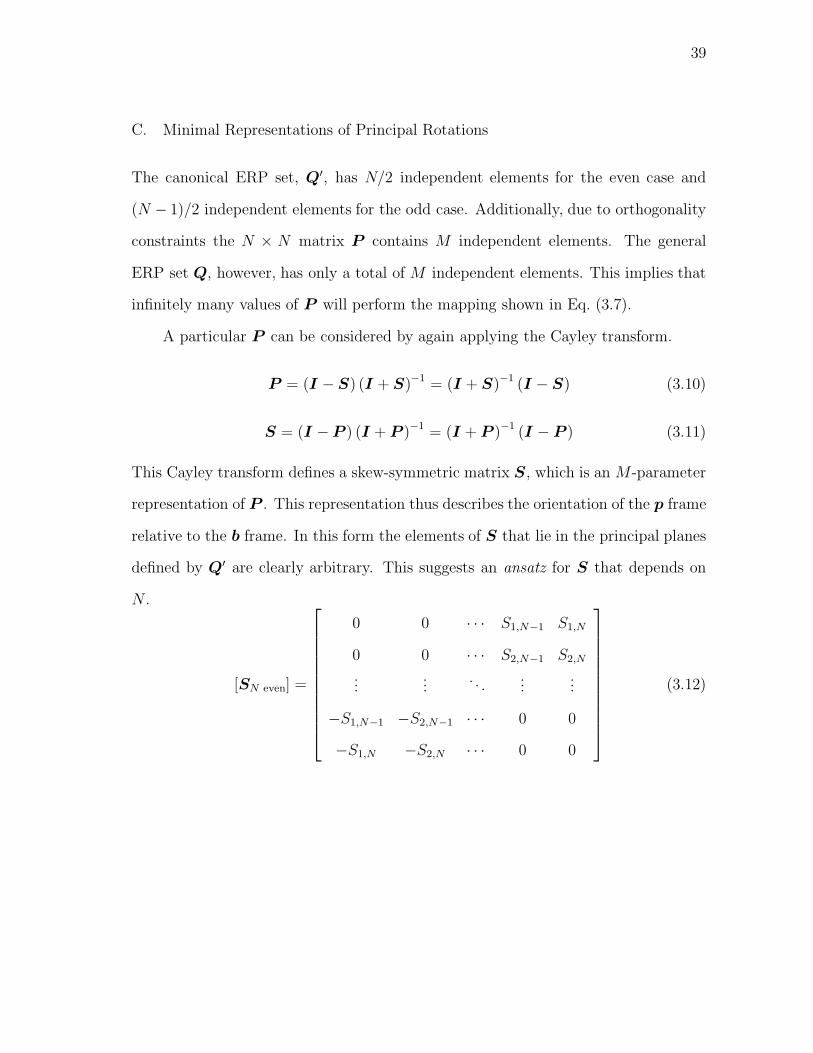
C. Minimal Representations of Principal Rotations

The canonical ERP set, Q′, has N/2 independent elements for the even case and

(N − 1)/2 independent elements for the odd case. Additionally, due to orthogonality

constraints the N × N matrix P contains M independent elements. The general

ERP set Q, however, has only a total of M independent elements. This implies that

infinitely many values of P will perform the mapping shown in Eq. (3.7).

A particular P can be considered by again applying the Cayley transform.

P = (I −S) (I + S)−1 = (I + S)−1 (I − S) (3.10)

S = (I −P ) (I + P )−1 = (I + P )−1 (I − P ) (3.11)

This Cayley transform defines a skew-symmetric matrix S, which is an M-parameter

representation of P . This representation thus describes the orientation of the p frame

relative to the b frame. In this form the elements of S that lie in the principal planes

defined by Q′ are clearly arbitrary. This suggests an ansatz for S that depends on

N .

[SN even] =

⎡⎢⎢⎢⎢⎢⎢⎢⎢⎢⎢⎣

0 0 · · · S1,N−1 S1,N

0 0 · · · S2,N−1 S2,N

......

. . ....

...

−S1,N−1 −S2,N−1 · · · 0 0

−S1,N −S2,N · · · 0 0

⎤⎥⎥⎥⎥⎥⎥⎥⎥⎥⎥⎦(3.12)

40

[SN odd]=

⎡⎢⎢⎢⎢⎢⎢⎢⎢⎢⎢⎢⎢⎢⎢⎣

0 0 · · · S1,N−2 S1,N−1 S1,N

0 0 · · · S2,N−2 S2,N−1 S2,N

......

. . ....

......

−S1,N−2 −S2,N−2 · · · 0 0 SN−2,N

−S1,N−1 −S2,N−1 · · · 0 0 SN−1,N

−S1,N −S2,N · · · −SN−2,N −SN−1,N 0

⎤⎥⎥⎥⎥⎥⎥⎥⎥⎥⎥⎥⎥⎥⎥⎦(3.13)

The off-diagonal elements that are non-zero in Q′ are arbitrarily set to zero in S,

whereas the off-diagonal elements that are zero in Q′ are non-zero in S. The elements

of these two matrices therefore combine to form a minimum-parameter (i.e., M-

parameter) orientation representation in terms of the principal rotations. For any

particular value of Q, the associated Q′ and S can be found by substituting the

assumed forms for these matrices (Eqs. (3.8) and (3.12) for even N and similar for

odd N) into Eq. (3.7). Using Eq. (3.10) to expand Eq. (3.7) gives the following.

Q′ = (I − S) (I + S)−1 Q (I − S)−1 (I + S) (3.14)

Evaluating these equations and setting the appropriate elements of Q′ to zero provides

M − N/2 (for even N) or M − (N − 1)/2 (for odd N) equations for the non-zero

elements of S. This process is straightforward but for large values of N the expanded

product in Eq. (3.14) can clearly involve a large number of terms. The equations

can be easily developed, however, using a symbolic manipulator such as Maple. Once

obtained, the equations are solved for the non-zero elements of S corresponding to

any particular value of Q. These elements can then be substituted into Eq. (3.14) to

produce the non-zero elements of Q′. It will be seen that for N = 3 the solution for

S can be obtained analytically, and simulation results for higher dimensions indicate

that a solution can be obtained numerically for general N .

41

The equations for the elements of S for N = 3 are developed as follows. The

Rodrigues parameters have the form shown below.

[Q] =

⎡⎢⎢⎢⎢⎣0 Q12 Q13

−Q12 0 Q23

−Q13 −Q23 0

⎤⎥⎥⎥⎥⎦ (3.15)

For the sake of generality in notation, the components of Q are retained in their

matrix notation instead of applying the vector notation specialized for N = 3. For

this case Q′ and S have the following forms.

[Q′] =

⎡⎢⎢⎢⎢⎣0 Q′

12 0

−Q′12 0 0

0 0 0

⎤⎥⎥⎥⎥⎦ ; [S] =

⎡⎢⎢⎢⎢⎣0 0 S13

0 0 S23

−S13 −S23 0

⎤⎥⎥⎥⎥⎦ (3.16)

From this form of S the Cayley transform is used to find P .

[P ] =1

1+S213+S

223

⎡⎢⎢⎢⎢⎣1 − S2

13 + S223 −2S13S23 −2S13

−2S13S23 1 + S213 − S2

23 −2S23

2S13 2S23 1 − S213 − S2

23

⎤⎥⎥⎥⎥⎦ (3.17)

This, of course, is similar to the general expression for a rotation matrix in terms of

a Rodrigues parameter set (with one identically-zero parameter). The elements of Q

and S are related to the elements of Q′, and Eqs. (3.15) and (3.17) are substituted

into Eq. (3.7). This product can be expanded to produce the elements of Q′. Setting

Q′13 and Q′

23 to zero yields the following two equations for the two unknown elements

of S.

2Q12S23 +Q13S213 + 2Q23S23S13 −Q13S

223 +Q13 = 0 (3.18)

2Q12S13 +Q23S213 − 2Q13S23S13 −Q23S

223 −Q23 = 0 (3.19)

42

For this case of N = 3 these equations can be solved analytically. First, for the

situation Q12 = Q13 = Q23 = 0, infinitely many solutions exist: S13 ∈ and S23 ∈ .

For this case there is no rotation, and any plane can be considered the principal plane.

Next, for the situation Q12 = 0 and Q13 = Q23 = 0 the equations admit a unique

solution: S13 = S23 = 0. For this case the rotation is in the (b1, b2) body plane, and

the principal frame is aligned with the body frame.

Two additional special cases can be solved directly from Eqs. (3.18) and (3.19).

For Q13 =0 and Q23 =0 two real solutions exist: S13 =(−Q12±√Q2

12+Q223)/Q23 and

S23 = 0. For Q13 = 0 and Q23 = 0 there are also two real solutions: S13 = 0 and

S23 =(Q12 ±

√Q2

12 +Q213

)/Q13.

The remaining general case of Q13 = 0 and Q23 = 0 can be solved by computing

the Grobner basis [18] of Eqs. (3.18) and (3.19). The result of this computation with

stronger weight on S13 is a factorable, fourth-order polynomial in S23 and a second

polynomial linear in S13.

[(Q2

13 +Q223

)S2

23 − 2Q12Q13S23 −Q213

]× [(Q2

13 +Q223

)S2

23 − 2Q12Q13S23 +Q212 +Q2

23

]= 0 (3.20)

(Q3

13Q23 +Q13Q323 +Q2

12Q13Q23

)S13 +Q12Q

313 +

(Q2

13 +Q223

)2S3

23

−3Q12Q13

(Q2

13 +Q223

)S2

23 +(Q2

12

(2Q2

13 +Q223

)−Q413 +Q4

23

)S23 = 0 (3.21)

The real solutions of Eq. (3.20) are shown below.

S23 =Q12Q13 ±Q13

√Q2

12 +Q213 +Q2

23

Q213 +Q2

23

(3.22)

Associated with each real solution of S23 there is a unique solution for S13 from

Eq. (3.21). Therefore Eqs. (3.18) and (3.19) have, in general, two real solutions

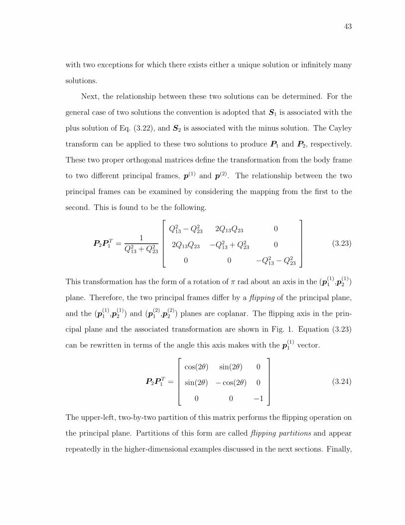
43

with two exceptions for which there exists either a unique solution or infinitely many

solutions.

Next, the relationship between these two solutions can be determined. For the

general case of two solutions the convention is adopted that S1 is associated with the

plus solution of Eq. (3.22), and S2 is associated with the minus solution. The Cayley

transform can be applied to these two solutions to produce P1 and P2, respectively.

These two proper orthogonal matrices define the transformation from the body frame

to two different principal frames, p(1) and p(2). The relationship between the two

principal frames can be examined by considering the mapping from the first to the

second. This is found to be the following.

P2PT1 =

1

Q213 +Q2

23

⎡⎢⎢⎢⎢⎣Q2

13 −Q223 2Q13Q23 0

2Q13Q23 −Q213 +Q2

23 0

0 0 −Q213 −Q2

23

⎤⎥⎥⎥⎥⎦ (3.23)

This transformation has the form of a rotation of π rad about an axis in the (p(1)1 ,p

(1)2 )

plane. Therefore, the two principal frames differ by a flipping of the principal plane,

and the (p(1)1 ,p

(1)2 ) and (p

(2)1 ,p

(2)2 ) planes are coplanar. The flipping axis in the prin-

cipal plane and the associated transformation are shown in Fig. 1. Equation (3.23)

can be rewritten in terms of the angle this axis makes with the p(1)1 vector.

P2PT1 =

⎡⎢⎢⎢⎢⎣cos(2θ) sin(2θ) 0

sin(2θ) − cos(2θ) 0

0 0 −1

⎤⎥⎥⎥⎥⎦ (3.24)

The upper-left, two-by-two partition of this matrix performs the flipping operation on

the principal plane. Partitions of this form are called flipping partitions and appear

repeatedly in the higher-dimensional examples discussed in the next sections. Finally,

44

θ

θ

2θ

p(1)

a

2

p(1)1

p(2)1

p(2)2

Fig. 1. Coordinatization of the principal plane by p(1) and p(2) frames, which are

related by a flipping about the axis a.

the angle θ can be found from the elements of Q.

θ =1

2tan−1

(2Q13Q23

Q213 −Q2

23

)(3.25)

So far, the analytical solution for the minimal-parameter representation was de-

scribed for N = 3 as well as the relationship between the two solutions. Although

many superior attitude representations exist for three dimensions, these results will

serve as a basis for the study of higher-dimension representations in the following

sections. For these higher dimensions, analytic solutions have not been found, and

numerical analysis is discussed instead.

45

1. Numeric Analysis for N = 4

For the four-dimensional representation, equations for the non-zero elements of S are

generated by setting the Q′13, Q

′14, Q

′23, and Q′

24 elements of Eq. (3.14) to zero. The re-

sulting equations are fairly extended, however, and are not shown here. Additionally,

analytic solutions to these equations have not been found. Monte Carlo simulation

can be used, though, to gain some confidence in the existence of a solution.

A Monte Carlo simulation was performed to show that solutions for S exist for a

distribution of Q values. Random values were generated for the independent elements

of Q, and then a numerical solution process was employed to find S. Values for Q

were selected with a uniform distribution between −1000 and 1000. The convergence

of each trial was tested to show that each identically zero value of Q′ evaluated from

Q and the computed S was less than 10−8. Ten thousand trials were run, and each of

these cases successfully converged to an accurate solution. This gives some confidence,

at least in an engineering sense, in the existence of a solution in general.

More detailed numerical studies were performed for the following example [2].

[C] =

⎡⎢⎢⎢⎢⎢⎢⎢⎣

0.1003 0.2496 −0.8894 −0.3697

0.9593 −0.0238 −0.0153 0.2810

−0.1172 −0.8638 −0.3828 0.3059

−0.2366 0.4370 −0.2495 0.8311

⎤⎥⎥⎥⎥⎥⎥⎥⎦(3.26)

From this rotation matrix a set of ERPs is computed using the Cayley transform.

[Q] =

⎡⎢⎢⎢⎢⎢⎢⎢⎣

0 1.0600 1.3893 −0.1929

−1.0600 0 −1.5467 −0.1091

−1.3893 1.5467 0 −0.6849

0.1929 0.1091 0.6849 0

⎤⎥⎥⎥⎥⎥⎥⎥⎦(3.27)

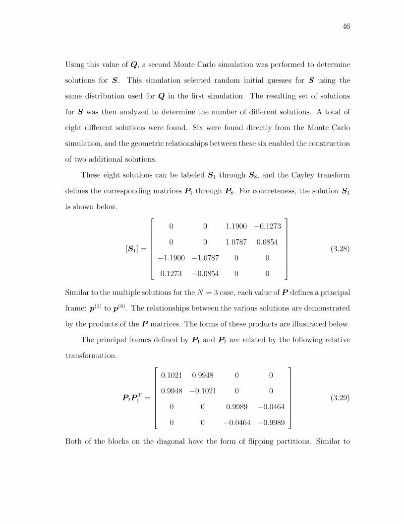
46

Using this value of Q, a second Monte Carlo simulation was performed to determine

solutions for S. This simulation selected random initial guesses for S using the

same distribution used for Q in the first simulation. The resulting set of solutions

for S was then analyzed to determine the number of different solutions. A total of

eight different solutions were found. Six were found directly from the Monte Carlo

simulation, and the geometric relationships between these six enabled the construction

of two additional solutions.

These eight solutions can be labeled S1 through S8, and the Cayley transform

defines the corresponding matrices P1 through P8. For concreteness, the solution S1

is shown below.

[S1] =

⎡⎢⎢⎢⎢⎢⎢⎢⎣

0 0 1.1900 −0.1273

0 0 1.0787 0.0854

−1.1900 −1.0787 0 0

0.1273 −0.0854 0 0

⎤⎥⎥⎥⎥⎥⎥⎥⎦(3.28)

Similar to the multiple solutions for the N = 3 case, each value of P defines a principal

frame: p(1) to p(8). The relationships between the various solutions are demonstrated

by the products of the P matrices. The forms of these products are illustrated below.

The principal frames defined by P1 and P2 are related by the following relative

transformation.

P2PT1 =

⎡⎢⎢⎢⎢⎢⎢⎢⎣

0.1021 0.9948 0 0

0.9948 −0.1021 0 0

0 0 0.9989 −0.0464

0 0 −0.0464 −0.9989

⎤⎥⎥⎥⎥⎥⎥⎥⎦(3.29)

Both of the blocks on the diagonal have the form of flipping partitions. Similar to

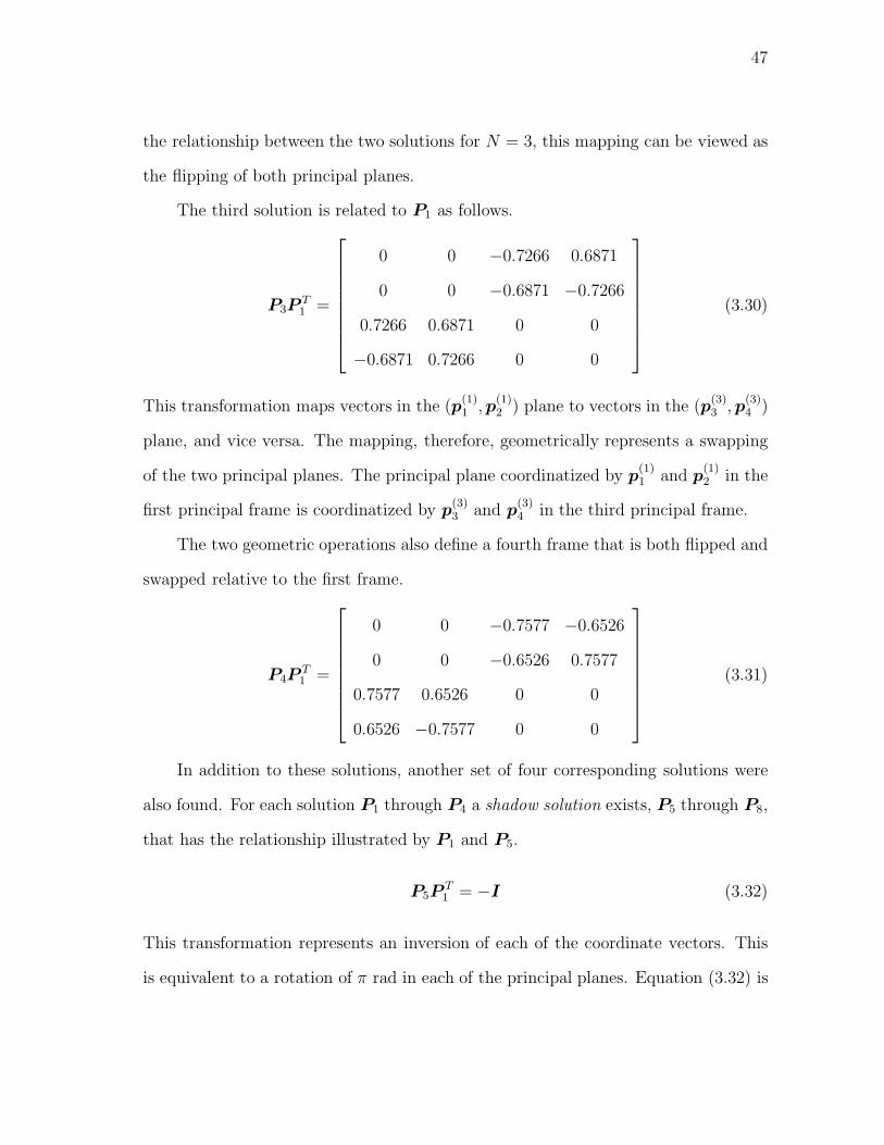
47

the relationship between the two solutions for N = 3, this mapping can be viewed as

the flipping of both principal planes.

The third solution is related to P1 as follows.

P3PT1 =

⎡⎢⎢⎢⎢⎢⎢⎢⎣

0 0 −0.7266 0.6871

0 0 −0.6871 −0.7266

0.7266 0.6871 0 0

−0.6871 0.7266 0 0

⎤⎥⎥⎥⎥⎥⎥⎥⎦(3.30)

This transformation maps vectors in the (p(1)1 , p

(1)2 ) plane to vectors in the (p

(3)3 , p

(3)4 )

plane, and vice versa. The mapping, therefore, geometrically represents a swapping

of the two principal planes. The principal plane coordinatized by p(1)1 and p

(1)2 in the

first principal frame is coordinatized by p(3)3 and p

(3)4 in the third principal frame.

The two geometric operations also define a fourth frame that is both flipped and

swapped relative to the first frame.

P4PT1 =

⎡⎢⎢⎢⎢⎢⎢⎢⎣

0 0 −0.7577 −0.6526

0 0 −0.6526 0.7577

0.7577 0.6526 0 0

0.6526 −0.7577 0 0

⎤⎥⎥⎥⎥⎥⎥⎥⎦(3.31)

In addition to these solutions, another set of four corresponding solutions were

also found. For each solution P1 through P4 a shadow solution exists, P5 through P8,

that has the relationship illustrated by P1 and P5.

P5PT1 = −I (3.32)

This transformation represents an inversion of each of the coordinate vectors. This

is equivalent to a rotation of π rad in each of the principal planes. Equation (3.32) is

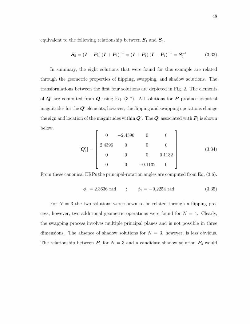
48

equivalent to the following relationship between S1 and S5.

S5 = (I −P5) (I + P5)−1 = (I + P1) (I − P1)

−1 = S−11 (3.33)

In summary, the eight solutions that were found for this example are related

through the geometric properties of flipping, swapping, and shadow solutions. The

transformations between the first four solutions are depicted in Fig. 2. The elements

of Q′ are computed from Q using Eq. (3.7). All solutions for P produce identical

magnitudes for the Q′ elements, however, the flipping and swapping operations change

the sign and location of the magnitudes within Q′. The Q′ associated with P1 is shown

below.

[Q′1] =

⎡⎢⎢⎢⎢⎢⎢⎢⎣

0 −2.4396 0 0

2.4396 0 0 0

0 0 0 0.1132

0 0 −0.1132 0

⎤⎥⎥⎥⎥⎥⎥⎥⎦(3.34)

From these canonical ERPs the principal-rotation angles are computed from Eq. (3.6).

φ1 = 2.3636 rad ; φ2 = −0.2254 rad (3.35)

For N = 3 the two solutions were shown to be related through a flipping pro-

cess, however, two additional geometric operations were found for N = 4. Clearly,

the swapping process involves multiple principal planes and is not possible in three

dimensions. The absence of shadow solutions for N = 3, however, is less obvious.

The relationship between P1 for N = 3 and a candidate shadow solution P3 would

49

represent a π-rad rotation in the principal plane.

P3PT1 =

⎡⎢⎢⎢⎢⎣−1 0 0

0 −1 0

0 0 1

⎤⎥⎥⎥⎥⎦ ≡ H (3.36)

From Eq. (3.7) this candidate solution would clearly produce the correct Q′.

P3QP T3 = HP1QP T

1 H = HQ′H = Q′ (3.37)

The matrix P1, however, satisfies the form given in Eq. (3.17). Applying the mapping

H to this form shows that P3 is a symmetric matrix. Therefore, each eigenvalue of P3

is either 1 or −1. Because each P is defined to be proper orthogonal, the eigenvalues

of P3 are either −1,−1, 1 or 1, 1, 1. If the eigenvalues are −1,−1, 1, then P3

represents a π-rad rotation away from the body frame and can not be described by

any corresponding S3 (i.e., the shadow solution is at infinity). If the eigenvalues are

1, 1, 1 then P3 is the identity matrix, and P1 = H . This, however, implies that

S1 does not exist and contradicts the results from the previous section. Therefore,

while shadow solutions for P exist for N = 3 they represent π-rad rotations from the

body frame and can not be described by a corresponding shadow S. For N = 4 the

application of −I produces no such symmetry in P .

2. Numeric Analysis for N = 5

Equations for the five-dimensional representation of S are generated by setting the

Q′13, Q

′14, Q

′15, Q

′23, Q

′24, Q

′25, Q

′35, and Q′

45 elements of Eq. (3.14) to zero. The re-

sulting equations are easily generated symbolically, however, they are fairly extended

and are not shown here. Again, analytic solutions to these equations have not been

50

Fig. 2. Relationships between four of the eight solutions for N = 4: f - flip, s - swap,

fs - flip and swap.

found. Monte Carlo simulation can be used, though, to gain some confidence in the

existence of a solution.

Similar to the four-dimensional case, a Monte Carlo simulation was performed

to show that solutions for S exist for a distribution of Q values. Random values were

generated for the independent elements of Q, and then a numerical solution process

was employed to find S. Values for Q were selected using the same distribution as

the four-dimensional case, and the converged solutions were checked using the same

test of numerical accuracy. Again ten thousand trials were run, and each of these

cases successfully converged to an accurate solution.

Similar to the four-dimensional case a more detailed numerical study of the

following example was performed.

[C] =

⎡⎢⎢⎢⎢⎢⎢⎢⎢⎢⎢⎣

−0.5708 −0.2224 0.4317 −0.2972 −0.5917

0.6799 −0.6616 0.1856 −0.1815 −0.1806

0.4241 0.6000 −0.0183 0.0554 −0.6758

−0.0505 −0.0280 −0.6987 −0.7067 −0.0955

−0.1719 −0.3899 −0.5392 0.6134 −0.3892

⎤⎥⎥⎥⎥⎥⎥⎥⎥⎥⎥⎦(3.38)

51

From this rotation matrix a set of ERPs is again computed using the Cayley trans-

form.

[Q] =

⎡⎢⎢⎢⎢⎢⎢⎢⎢⎢⎢⎣

0 2.8562 −0.3120 −0.1737 1.4409

−2.8562 0 0.7635 0.7395 −1.5106

0.3120 −0.7635 0 −2.1241 0.8507

0.1737 −0.7395 2.1241 0 2.4560

−1.4409 1.5106 −0.8507 −2.4560 0

⎤⎥⎥⎥⎥⎥⎥⎥⎥⎥⎥⎦(3.39)

Another Monte Carlo simulation was performed using this value of Q to attempt

to find multiple solutions for S. Initial guesses for S were selected from the same

distribution used previously, and the results from the numerical solution procedure

were analyzed. A total of sixteen solutions were found for this example. Thirteen

solutions were found directly from the Monte Carlo simulation, and three more were

constructed from the geometric relations implied by the thirteen. For concreteness

the solution S1 is shown below.

[S1] =

⎡⎢⎢⎢⎢⎢⎢⎢⎢⎢⎢⎣

0 0 −0.3111 0.1450 −0.4123

0 0 0.0959 0.3898 −0.2318

0.3111 −0.0959 0 0 −0.3816

−0.1450 −0.3898 0 0 0.0551

0.4123 0.2318 0.3816 −0.0551 0

⎤⎥⎥⎥⎥⎥⎥⎥⎥⎥⎥⎦(3.40)

The rotation matrix, P1, associated with S1 is computed using the Cayley transform.

Because the fifth axis of the principal frame was chosen to be aligned with the principal

axis, the fifth column of every P T (the fifth row of P ) is aligned with the principal

axis in body coordinates.

In addition to the flipping, swapping, and shadow solutions observed for N = 4

a new geometric relationship was found for the N = 5 case. The new geometric oper-

52

ation is a flipping of one principal plane and a rotation in the other principal plane.

Defining P2 to be a flipped-rotated solution relative to P1, the relative transformation

matrix was found to be the following.

P2PT1 =

⎡⎢⎢⎢⎢⎢⎢⎢⎢⎢⎢⎣

−0.4203 −0.9074 0 0 0

−0.9074 0.4203 0 0 0

0 0 0.8879 −0.4601 0

0 0 0.4601 0.8879 0

0 0 0 0 −1

⎤⎥⎥⎥⎥⎥⎥⎥⎥⎥⎥⎦(3.41)

Here, the (1-2,1-2) block has the form of a flipping partition. The (3-4,3-4) block,

however, has the form of a rotation in a plane and is a rotation partition. Another

solution, P3, is related to P1 by a rotation in the first principal plane and a flipping

of the second plane. The relative transformation for this rotated-flipped solution is

similar.

P3PT1 =

⎡⎢⎢⎢⎢⎢⎢⎢⎢⎢⎢⎣

0.8600 0.5103 0 0 0

−0.5103 0.8600 0 0 0

0 0 −0.9952 0.0977 0

0 0 0.0977 0.9952 0

0 0 0 0 −1

⎤⎥⎥⎥⎥⎥⎥⎥⎥⎥⎥⎦(3.42)

Similar to the N = 4 case another solution exists that is related by a flipping of both

principal planes.

53

P4PT1 =

⎡⎢⎢⎢⎢⎢⎢⎢⎢⎢⎢⎣

−0.6301 0.7765 0 0 0

0.7765 0.6301 0 0 0

0 0 −0.9743 −0.2253 0

0 0 −0.2253 0.9743 0

0 0 0 0 1

⎤⎥⎥⎥⎥⎥⎥⎥⎥⎥⎥⎦(3.43)

The relationships between the first four solutions are summarized in Fig. 3.

In addition to these four solutions another four solutions are related to P1 by

a swapping of the principal planes. These relative transformations contain either a

flipping or rotation partition in the (1-2,3-4) and (3-4,1-2) blocks and a positive or

negative one in the (5, 5) element. Each of these eight solutions also has a shadow

solution that is related by the following relative transformation.

P9PT1 =

⎡⎢⎢⎢⎢⎢⎢⎢⎢⎢⎢⎣

−1 0 0 0 0

0 −1 0 0 0

0 0 −1 0 0

0 0 0 −1 0

0 0 0 0 1

⎤⎥⎥⎥⎥⎥⎥⎥⎥⎥⎥⎦(3.44)

Similar to the N = 4 case, this transformation performs a π-rad rotation in both

principal planes.

The existence of flipped-rotated and rotated-flipped solutions for N = 5 but not

N = 4 is related to the differences in sign of the (5, 5) elements of Eqs. (3.41) to

(3.43). Because P is defined as a proper orthogonal matrix, the relative transfor-

mation between two solutions must also be proper. The determinant of the relative

transformation will be equal to the product of the eigenvalues of each of the blocks

on the diagonal. The product of the eigenvalues of a rotation partition is positive

one. The product of the eigenvalues of a flipping partition, however, is negative one.

54

Fig. 3. Relationships between four of the sixteen solutions for N = 5: fr - flip-rotate,

rf - rotate-flip, ff - flip-flip.

For N = 4 a double-flipping relative transformation has two blocks with negative

one determinants and results in an overall proper transformation. For N = 5 the

double flip can be accompanied by an identity transformation of the principal axis to

also result in a proper transformation. The presence of the principal axis, however,

introduces another possibility. A single flip and a rotate can be accompanied by an

inversion of the principal axis to preserve properness. In even spaces flips must appear

in pairs, but in odd spaces flips can either appear in pairs or appear singly along with

inversion of the principal axis.

From P and Q the elements of Q′ can once again be computed using Eq. (3.7).

The matrix Q′1 is shown below.

[Q′1] =

⎡⎢⎢⎢⎢⎢⎢⎢⎢⎢⎢⎣

0 4.0838 0 0 0

−4.0838 0 0 0 0

0 0 0 −2.8920 0

0 0 2.8920 0 0

0 0 0 0 0

⎤⎥⎥⎥⎥⎥⎥⎥⎥⎥⎥⎦(3.45)

55

These canonical ERPs give the following principal rotation angles.

φ1 = −2.6613 rad ; φ2 = 2.4758 rad (3.46)

D. Discussion

For N = 3 the Rodrigues parameters form a minimum-parameter attitude represen-

tation that is directly related to the principal-rotation description. The direct ex-

tension of these parameters to higher dimensions, the ERPs, maintain the minimum-

parameter property, however, they lose the direct connection to the principal ro-

tations. Historically, the connection between the ERPs and the principal-rotation

description has been established using eigenanalysis or canonical forms. These tech-

niques by themselves, however, destroy the minimum-parameter property. Through

the evaluation of Q′ and S this chapter has demonstrated one method of describing

the principal rotations while maintaining a minimum-parameter representation. Per-

haps most usefully, these matrices provide an interpretation for the ERP elements.

Because these matrices form an orientation representation it should be possible to

develop kinematic equations to directly relate their derivatives to the N -dimensional

angular velocity. A result as elegant as the Cayley-transform kinematic relations for

the ERP rates, however, is not anticipated, and the idea is not pursued further in

this dissertation.

The evaluation of Q′ and S that has been presented is similar to the eigenanal-

ysis of C because both methods produce the principal angles, principal planes, and

principal axis (if it exists) of any arbitrary orientation. The key difference between

these two approaches comes in the representation of the principal planes. An impor-

tant aspect of the canonical ERPs is that they provide a principal frame in which

the various principal rotations become geometrically decoupled. This is a useful tool

56

for describing N -dimensional orientations and relating them to the more familiar two

and three-dimensional rotations. In particular this could be applied to the study of

mechanical-system dynamics and control as represented by N -dimensional rotations.

57

CHAPTER IV

HAMEL COEFFICIENTS FOR THE ROTATIONAL MOTION OF AN

N -DIMENSIONAL RIGID BODY∗

A. Introduction

Although the field of mechanics has focused on continua and rigid bodies existing

in three-dimensional space, there has also been interest in extending the principles

that have been discovered to higher dimensions. In particular, methods have been

developed to describe the orientation, rotation, and angular velocity of N -dimensional

rigid bodies [2, 5–7, 10, 12, 19]. Work has also been done on developing the equations

that govern the motion of rigid bodies in higher-dimensional spaces. In this regard,

the primary focus has been on different representations of the equations and their

integrability.

The various forms of the N -dimensional dynamic equations reported in the lit-

erature were constructed using geometric methods, namely, the Hamiltonian method

of mechanics. This method takes a geometric view of mechanics, focusing on geomet-

ric structures called symplectic or Poisson structures [20]. These various forms were

obtained from the accepted principle that, even in higher-dimensional spaces, the

time derivative of the angular-momentum matrix equals the applied skew-symmetric

matrix of torques; in the absence of torques, the time derivative of the angular-

momentum matrix equals zero.

According to Fedorov and Kozlov, the idea of generalizing the rigid-body rota-

tional equations was first put forth by Cayley [8,21]. The generalized Euler equations,

∗Reprinted with permission from “Hamel coefficients for the rotational motion ofan N -dimensional rigid body” by J. E. Hurtado and A. J. Sinclair, 2004. Proceedingsof the Royal Society of London Series A, 460, 3613–3630. 2004 by The Royal Society.

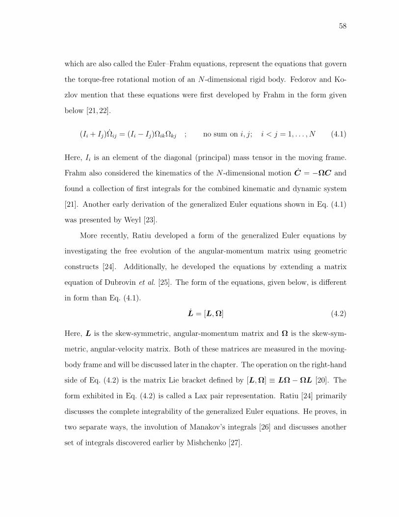
58

which are also called the Euler–Frahm equations, represent the equations that govern

the torque-free rotational motion of an N -dimensional rigid body. Fedorov and Ko-

zlov mention that these equations were first developed by Frahm in the form given

below [21, 22].

(Ii + Ij)Ωij = (Ii − Ij)ΩikΩkj ; no sum on i, j; i < j = 1, . . . , N (4.1)

Here, Ii is an element of the diagonal (principal) mass tensor in the moving frame.

Frahm also considered the kinematics of the N -dimensional motion C = −ΩC and

found a collection of first integrals for the combined kinematic and dynamic system

[21]. Another early derivation of the generalized Euler equations shown in Eq. (4.1)

was presented by Weyl [23].

More recently, Ratiu developed a form of the generalized Euler equations by

investigating the free evolution of the angular-momentum matrix using geometric

constructs [24]. Additionally, he developed the equations by extending a matrix

equation of Dubrovin et al. [25]. The form of the equations, given below, is different

in form than Eq. (4.1).

L = [L,Ω] (4.2)

Here, L is the skew-symmetric, angular-momentum matrix and Ω is the skew-sym-

metric, angular-velocity matrix. Both of these matrices are measured in the moving-

body frame and will be discussed later in the chapter. The operation on the right-hand

side of Eq. (4.2) is the matrix Lie bracket defined by [L,Ω] ≡ LΩ − ΩL [20]. The

form exhibited in Eq. (4.2) is called a Lax pair representation. Ratiu [24] primarily

discusses the complete integrability of the generalized Euler equations. He proves, in

two separate ways, the involution of Manakov’s integrals [26] and discusses another

set of integrals discovered earlier by Mishchenko [27].

59

Fedorov and Kozlov present a discussion on ‘viewing’ the free motion of an N -

dimensional rigid body [21]. A technique is presented in which one considers an

M-dimensional rigid body (M = N(N − 1)/2), called the kinematical body. The

kinematical body lends itself to being analyzed using a generalized Poinsot model,

but only in a limited way: the generalized Poinsot model can only provide information

about the positions of the kinematical body but not its motion.

Bloch et al. give a remarkable symmetric representation of the N -dimensional

rigid-body equations [28]. This representation arises from studying the free motion

of the N -dimensional rigid body as an optimal-control problem [29,30].

In this chapter, the equations of motion are developed for N -dimensional rigid

bodies from Lagrange’s equations using the angular-velocity components as quasi

velocities. Here an N -dimensional rigid body will be defined as a system whose con-

figuration can be completely defined by an N ×N proper orthogonal matrix. A wide

variety of dynamical systems can be modeled as N -dimensional rigid bodies using

this definition [16], which relaxes some conditions used in earlier work. The chapter

begins with a review of N -dimensional kinematics. Next, a new numerical relative

tensor, χjik, is introduced and defined to allow the expression of N -dimensional kine-

matics in index notation. This symbol is then used to compute the Hamel coefficients

for N -dimensional rotations. Finally, these coefficients allow the development of the

rotational equations of motion for general rigid bodies.

B. Review of N -Dimensional Kinematics

The kinematics of rigid bodies in N -dimensional spaces has been developed through

the work of many researchers. The transformation of an N -dimensional position

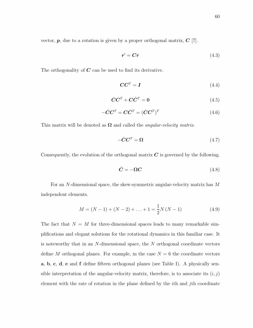
60

vector, p, due to a rotation is given by a proper orthogonal matrix, C [7].

r′ = Cr (4.3)

The orthogonality of C can be used to find its derivative.

CCT = I (4.4)

CCT + CCT = 0 (4.5)

−CCT = CCT = (CCT )T (4.6)

This matrix will be denoted as Ω and called the angular-velocity matrix.

−CCT = Ω (4.7)

Consequently, the evolution of the orthogonal matrix C is governed by the following.

C = −ΩC (4.8)

For an N -dimensional space, the skew-symmetric angular-velocity matrix has M

independent elements.

M = (N − 1) + (N − 2) + . . . + 1 =1

2N (N − 1) (4.9)

The fact that N = M for three-dimensional spaces leads to many remarkable sim-

plifications and elegant solutions for the rotational dynamics in this familiar case. It

is noteworthy that in an N -dimensional space, the N orthogonal coordinate vectors

define M orthogonal planes. For example, in the case N = 6 the coordinate vectors

a, b, c, d, e and f define fifteen orthogonal planes (see Table I). A physically sen-

sible interpretation of the angular-velocity matrix, therefore, is to associate its (i, j)

element with the rate of rotation in the plane defined by the ith and jth coordinate

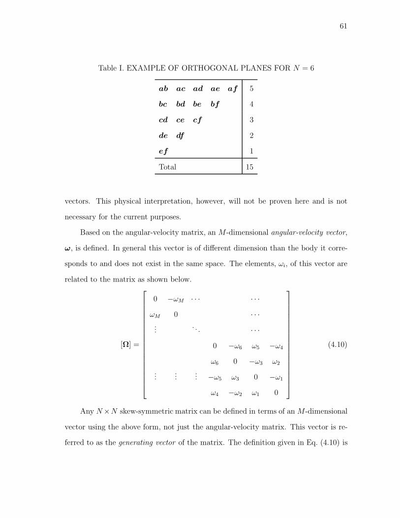
61

Table I. EXAMPLE OF ORTHOGONAL PLANES FOR N = 6

ab ac ad ae af 5

bc bd be bf 4

cd ce cf 3

de df 2

ef 1

Total 15

vectors. This physical interpretation, however, will not be proven here and is not

necessary for the current purposes.

Based on the angular-velocity matrix, an M-dimensional angular-velocity vector,

ω, is defined. In general this vector is of different dimension than the body it corre-

sponds to and does not exist in the same space. The elements, ωi, of this vector are

related to the matrix as shown below.

[Ω] =

⎡⎢⎢⎢⎢⎢⎢⎢⎢⎢⎢⎢⎢⎢⎢⎢⎢⎢⎣

0 −ωM · · · · · ·ωM 0 · · ·...

. . . · · ·0 −ω6 ω5 −ω4

ω6 0 −ω3 ω2

......

... −ω5 ω3 0 −ω1

ω4 −ω2 ω1 0

⎤⎥⎥⎥⎥⎥⎥⎥⎥⎥⎥⎥⎥⎥⎥⎥⎥⎥⎦

(4.10)

Any N×N skew-symmetric matrix can be defined in terms of an M-dimensional

vector using the above form, not just the angular-velocity matrix. This vector is re-

ferred to as the generating vector of the matrix. The definition given in Eq. (4.10) is

62

somewhat arbitrary and is chosen to be consistent with the familiar three-dimensional

form. In that special case, multiplication of the angular-velocity matrix and any arbi-

trary vector is equivalent to taking the cross product of the angular-velocity vector and

the arbitrary vector. In general, however, this is not true. The general N -dimensional

cross product can be represented as multiplication of a skew-symmetric matrix and

a vector, but the matrix is actually composed of N − 2 orthogonal, N -dimensional

vectors [19]. Therefore, these cross-product vectors have N(N − 2) elements subject

to P orthogonality constraints, leaving R independent elements.

P = (N − 3) + (N − 4) + . . .+ 1 =1

2N2 − 5

2N + 3 (4.11)

R = N(N − 2) − P =1

2N2 +

1

2N − 3 (4.12)

The facts that for N = 3, one has N = M = R and the single cross-product

vector is the angular-velocity vector, are additional remarkable properties of rotational

motion in three dimensions. For higher dimensions, R is larger than M and multiple

cross-product vectors give the same skew-symmetric, angular-velocity matrix. This

makes it difficult to use these vectors to parameterize the angular velocity of an N -

dimensional body. If a method could be found, however, to select a particular set

of cross-product vectors, then it seems possible to study N -dimensional rotations in

terms of these vectors. This idea is not pursued further in this dissertation.

C. Definition of the Numerical Relative Tensor χjik

For the derivations in the subsequent sections it will be useful to have a compact form

in index notation to describe the relations between the elements of ω and Ω given by

Eq. (4.10). For N = 3 this is given by the Levi-Civita permutation symbol [31].

Ωik = εijkωj (4.13)

63

For N -dimensions a new symbol, χjik, must be defined that will perform the same

operation as εijk in the three-dimensional case.

Ωik = χjikωj (4.14)

Like εijk, the symbol χjik is a numerical relative tensor [32]. It is a generalization of

the Levi-Civita symbol that for the case N = 3 simplifies to εijk. The symbol χjik

is not, however, the generalized Levi-Civita symbol discussed by Papastavridis and

others [33, 34]. Also, whereas here χjik is used to relate the angular-velocity matrix

and vector, it can be used with any skew-symmetric matrix and its generating vector.

In this section some properties of this new numerical relative tensor will be examined.

First, it is important to notice that in Eq. (4.14) the index j is summed from 1 to

M , whereas the indices i and k take on values from 1 to N . It is another remarkable

and elegant property of the N = 3 case that the number of indices of χjik (always

three) is equal to the range of each of the indices (three only for N = 3). From

examination of Eq. (4.10) the values of χjik are clearly limited to +1, −1, and 0.

Additionally it is clear that for a particular value of i and k, at most one value of j

will give a nonzero value of χjik.

Another property of χjik can be deduced from the skew-symmetry of Ω.

Ωik = −Ωki

χjikωj = −χj

kiωj(χj

ik + χjki

)ωj = 0

χjik = −χj

ki (4.15)

The final step above holds because the elements ωj are independent. Equation (4.15)

demonstrates that if i = k, then χjik equals zero for all values of j.

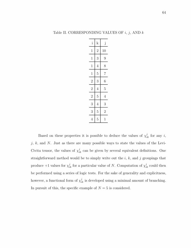
64

Table II. CORRESPONDING VALUES OF i, j, AND k

i k j

1 2 10

1 3 9

1 4 8

1 5 7

2 3 6

2 4 5

2 5 4

3 4 3

3 5 2

4 5 1

Based on these properties it is possible to deduce the values of χjik for any i,

j, k, and N . Just as there are many possible ways to state the values of the Levi-

Civita tensor, the values of χjik can be given by several equivalent definitions. One

straightforward method would be to simply write out the i, k, and j groupings that

produce +1 values for χjik for a particular value of N . Computation of χj

ik could then

be performed using a series of logic tests. For the sake of generality and explicitness,

however, a functional form of χjik is developed using a minimal amount of branching.

In pursuit of this, the specific example of N = 5 is considered.

65

From Table II one observes that for a particular value of i, the largest value of j

is given by the following.

jmax = (N − i) + (N − i− 1) + . . .+ 1

= (N − i) +1

2

[(N − i)2 − (N − i)

](4.16)

=1

2

[(N − i)

2+ (N − i)

]For these values of i and j, the value of k is i + 1 and this is seen to be the min-

imum value of k. As k increases, j decreases from the maximum value given by

Eq. (4.16). Therefore, the following relationship holds between i, j, and k for which

χjik = (−1)i+k.

j =1

2

[(N − i)2 + (N − i)

]+ (i+ 1) − k (4.17)

=1

2i2 +

(1

2−N

)i− k +

1

2N2 +

1

2N + 1

In developing the above relationship the upper-triangular elements of the skew-sym-

metric matrix were considered, assuming k > i. To use this expression for any element

of the matrix, the pair k and i must be replaced with the pair x and y, where x is

the larger value of the original pair and y is the smaller. In expressing x, y, and χjik,

a useful function is f(i, k) which returns +1 for k > i and −1 for k < i.

f(i, k) =k − i√(k − i)2

(4.18)

Therefore the form of χjik is given by the following expression, which happens to be a

function of the dimension N because of the form chosen in Eq. (4.10).

66

χjik =

⎧⎪⎨⎪⎩ (−1)i+k f(i, k) for j = z and i = k

0 otherwise(4.19)

where x =1

2

(i+ k +

√(k − i)2

); y =

1

2

(i+ k −

√(k − i)2

);

z =1

2y2 +

(1

2−N

)y−x+

1

2N2 +

1

2N + 1

The inverse of χjik will also be considered. Equations (4.14) and (4.19) provide

a mapping or sorting of the elements of a generating vector into the elements of

the skew-symmetric matrix. The mapping from the matrix elements to the vector

elements can also be considered. To accomplish this the numerical relative tensor ψjik

is introduced which satisfies the following equation.

ωj = ψjikΩik (4.20)

Equation (4.14) can be substituted into the above equation.

δjlωl = ψjikχ

likωl(

δjl − ψjikχ

lik

)ωl = 0

ψjikχ

lik = δjl (4.21)

Therefore ψjik can be considered the inverse of χl

ik. The properties of ψjik can

now be investigated similar to χjik. First note, however, that Eq. (4.20) represents

a mapping of N2 matrix elements onto M vector elements. Therefore Eq. (4.20)

does not completely define ψjik and several additional properties must be arbitrarily

chosen to uniquely define ψjik. In particular, ψj

ik is selected such that it is nonzero

if and only if the combination i, j and k produces a nonzero value of χjik and such

that ψjik = −ψj

ki. This implies that in the summation of Eq. (4.20), elements Ωik not

67

containing ±ωj will be multiplied by a coefficient ψjik = 0. Equation (4.10) therefore

shows that only two nonzero terms of Eq. (4.20) will exist for any value of j. These

terms will correspond with some pair of particular values i and k, and the summation

in Eq. (4.20) can be written explicitly as the following.

ωj = ψjikΩik + ψj

kiΩki (no sum on i, j, and k)

= ψjikχ

jikωj + ψj

kiχjkiωj

=(ψj

ikχjik + ψj

kiχjki

)ωj (4.22)

Consequently, because the elements ωj can be nonzero, the following equation must

hold.

ψjikχ

jik + ψj

kiχjki = 1 (no sum on i, j, and k) (4.23)

Without the loss of generality, it may be assumed that the current values of i, j, and

k produce χjik = 1 and χj

ki = −1. Additionally, it is true that ψjik must equal some

nonzero value α, whereas ψjki must equal −α.

(α) (1) + (−α) (−1) = 1 =⇒ α =1

2(4.24)

Thus Eq. (4.24) and the above definitions show that for any possible values of i, j,

and k the inverse symbol ψjik is equal to half of χj

ik. Therefore the ψjik notation is

dropped as redundant, leaving the following useful relations.

Ωik = χjikωj

ωj =1

2χj

ikΩik

1

2χj

ikχlik = δjl (4.25)

In fact, Eq. (4.25) can be derived without explicitly introducing the inverse tensor,

as shown in Appendix A.

68

Several additional useful properties of χjik can be established. The first is a

generalization of the ‘ε-δ identity’: εijkεimn = δjmδkn − δjnδkm. For N -dimensional

systems the following ‘χ-δ identity’ will be proven.

χijkχ

imn = δjmδkn − δjnδkm ≡ δjk

mn (4.26)

The symbol on the far right-hand side of Eq. (4.26) is the generalized Kronecker

delta [32]. Consider the inner-product of two arbitrary generating vectors, u and v.

This product can be written in terms of the related skew-symmetric tensors.

uivi =

(1

2χi

jkUjk

)(1

2χi

mnVmn

)=

1

4χi

jkχimnUjkVmn (4.27)

This inner-product can also be written in the following manner.

uivi =

(1

2χi

jkUjk

)vi =

1

2UjkVjk (4.28)

Comparing equations (4.27) and (4.28) and using Kronecker delta substitution gives

the following result.

1

2χi

jkχimnUjkVmn = UjkVjk = δjmδknUjkVmn (4.29)

Due to the skew-symmetry of U one can also write the following.

1

2χi

jkχimnUjkVmn = −UkjVjk = −δjnδkmUkjVnm = −δjnδkmUjkVmn (4.30)

Next, equations (4.29) and (4.30) are summed.

χijkχ

imnUjkVmn = (δjmδkn − δjnδkm)UjkVmn (4.31)

[χi

jkχimn − (δjmδkn − δjnδkm)

] UjkVmn = 0 (4.32)

69

Equation (4.32) represents a series summing on the indices j, k, m, and n, and for

convenience is rewritten in the following manner.

[cjkmn] xjkmn = 0 (4.33)

Because the elements xjkmn are not independent, the coefficients in the square brackets

can not be set immediately to zero. The elements of xjkmn have a certain structure

due to the skew-symmetry of U and V described by the following two properties: (1)

some elements xjkmn are identically zero; (2) certain elements of xjkmn are related to

each other.

The first property implies that for particular values of j, k, m, and n the value

of cjkmn can not be determined from Eq. (4.33). These values, however, can be

determined from direct evaluation of cjkmn. An element xjkmn will be identically

equal to zero if j = k or m = n. In either of these cases, Eq. (4.32) shows that one

has cjkmn = 0.

The second property implies that certain terms of the series in Eq. (4.33) will

be related to each other. A four-term subseries of the summation in Eq. (4.33) is

explicitly written below for particular values of j, k, m, and n.

cjkmnxjkmn + ckjmnxkjmn + cjknmxjknm + ckjnmxkjnm (4.34)

= (cjkmn − ckjmn − cjknm + ckjnm)xjkmn (no sum on j, k, m, and n)

In writing the above equation the skew-symmetry of U and V were again used to

switch indices of the elements xjkmn. The parenthetical term above can be simplified

70

using the definition of cjkmn.

cjkmn − ckjmn − cjknm + ckjnm (no sum on j, k, m, and n)

=[χi


]− [χikjχ

imn − (δkmδjn − δknδjm)

]− [χi

jkχinm − (δjnδkm − δjmδkn)

]+[χi

kjχinm − (δknδjm − δkmδjn)

]= 4

[χi


]= 4 cjkmn (4.35)

Thus, the subseries of related terms can be written as 4 (cjkmn) (xjkmn) (no sum on j,

k, m, and n).

Using this result, the series in Eq. (4.33) can be expressed in the following con-

densed form.

[cjkmn] yjkmn = 0 ; j ≤ k; m ≤ n (4.36)

In this form, certain elements of yjkmn are identically zero but are otherwise arbitrary.

For the terms yjkmn = 0 it has been shown that cjkmn = 0; for the nonzero elements

of yjkmn, it must then be that cjkmn = 0 for j ≤ k and m ≤ n. By the skew-symmetry

properties illustrated in Eq. (4.35) one can see that this implies cjkmn = 0 for all j,

k, m, and n, and the proof of Eq. (4.26) is complete.

Setting the index m equal to j in the χ-δ identity reveals another property.

χijkχ

ijn = δjjδkn − δjnδkj = (N − 1) δkn (4.37)

The properties of the χjik are summarized in Table III. As mentioned earlier, χj

ik

is a generalization of the Levi-Civita permutation symbol. Due to the properties of

N = 3 described in this and the previous sections, the Levi-Civita symbol combines

properties relating to permutations, the cross-product operation, and skew-symmetric

matrices. For higher dimensions, however, these properties become distinct and can

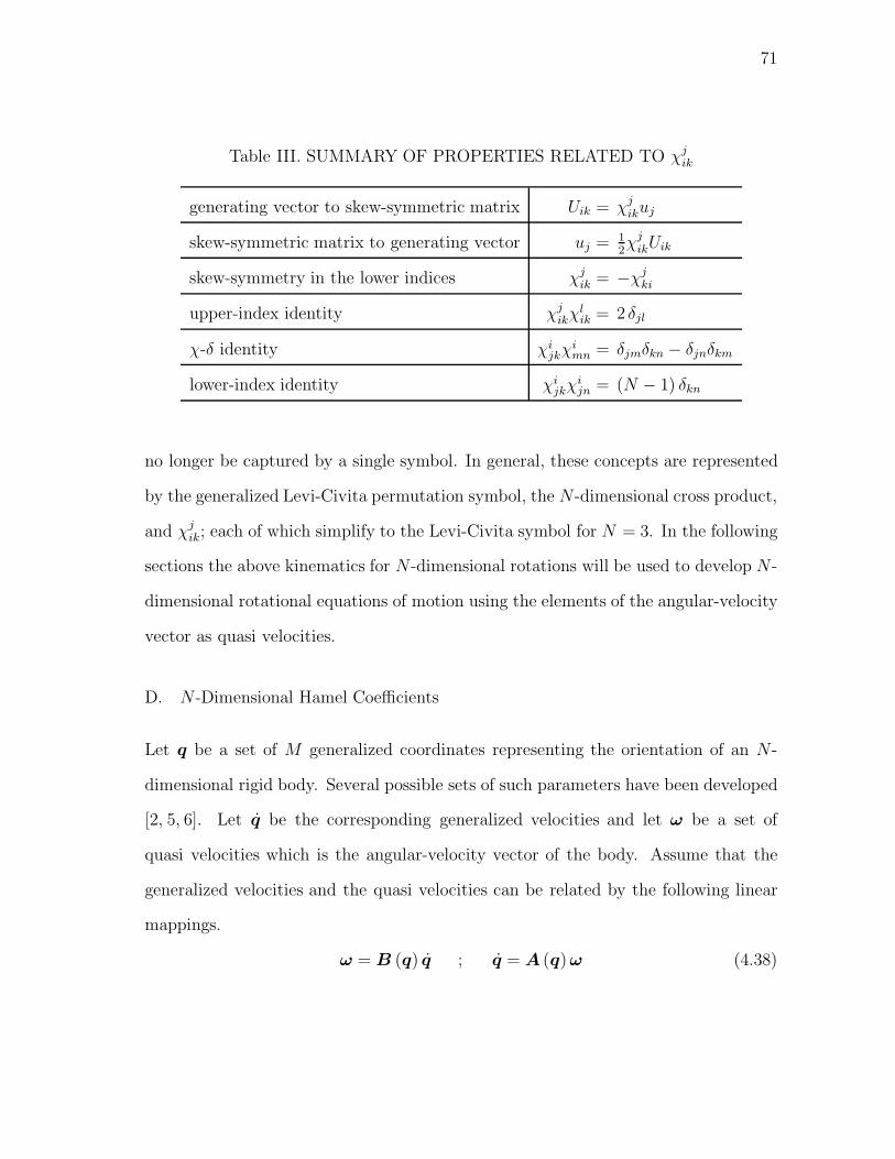
71

Table III. SUMMARY OF PROPERTIES RELATED TO χjik

generating vector to skew-symmetric matrix Uik = χjikuj

skew-symmetric matrix to generating vector uj = 12χj

ikUik

skew-symmetry in the lower indices χjik = −χj

ki

upper-index identity χjikχ

lik = 2 δjl

χ-δ identity χijkχ

imn = δjmδkn − δjnδkm

lower-index identity χijkχ

ijn = (N − 1) δkn

no longer be captured by a single symbol. In general, these concepts are represented

by the generalized Levi-Civita permutation symbol, the N -dimensional cross product,

and χjik; each of which simplify to the Levi-Civita symbol for N = 3. In the following

sections the above kinematics for N -dimensional rotations will be used to develop N -

dimensional rotational equations of motion using the elements of the angular-velocity

vector as quasi velocities.

D. N -Dimensional Hamel Coefficients

Let q be a set of M generalized coordinates representing the orientation of an N -

dimensional rigid body. Several possible sets of such parameters have been developed

[2, 5, 6]. Let q be the corresponding generalized velocities and let ω be a set of

quasi velocities which is the angular-velocity vector of the body. Assume that the

generalized velocities and the quasi velocities can be related by the following linear

mappings.

ω = B (q) q ; q = A (q)ω (4.38)

72

Lagrange’s equations of motion in terms of generalized coordinates and general-

ized velocities are shown below.

d

dt

(∂T0

∂qk

)− ∂T0

∂qk= f0k (4.39)

Lagrange’s equations of motion in terms of generalized coordinates and quasi veloc-

ities can also be established.

d

dt

(∂T1

∂ωk

)+ γr

kaωa∂T1

∂ωr− Ark

∂T1

∂qr= f1k (4.40)

Here, T = T0(q, q) and T = T1(q,ω) are two different functional forms of the same

kinetic-energy expression, and the generalized forces f1k are defined as f1k ≡ Arkf0r.

Equation (4.40) is simply called the Lagrange equations for quasi coordinates [35]. Re-

lated to these equations are the Euler-Poincare equations [20,36]. In one sense, the La-

grange equations for quasi coordinates are more general than the Euler-Poincare equa-

tions because the Euler-Poincare equations only apply to left-invariant Lagrangian

systems. On the other hand, the Euler-Poincare equations are more general because

they govern the motion of Lagrangian systems corresponding to general Lie groups.

The three-index symbol γrka that appears in Eq. (4.40) represents the Hamel

coefficients, which may be given by the following expression.

γrka ≡

(∂Brj

∂qi− ∂Bri

∂qj

)AjkAia (4.41)

These coefficients are also known as the Hamel–Volterra transitivity coefficients or

the Ricci–Boltzmann–Hamel three-index symbols [33]. Note that the Hamel coefficient

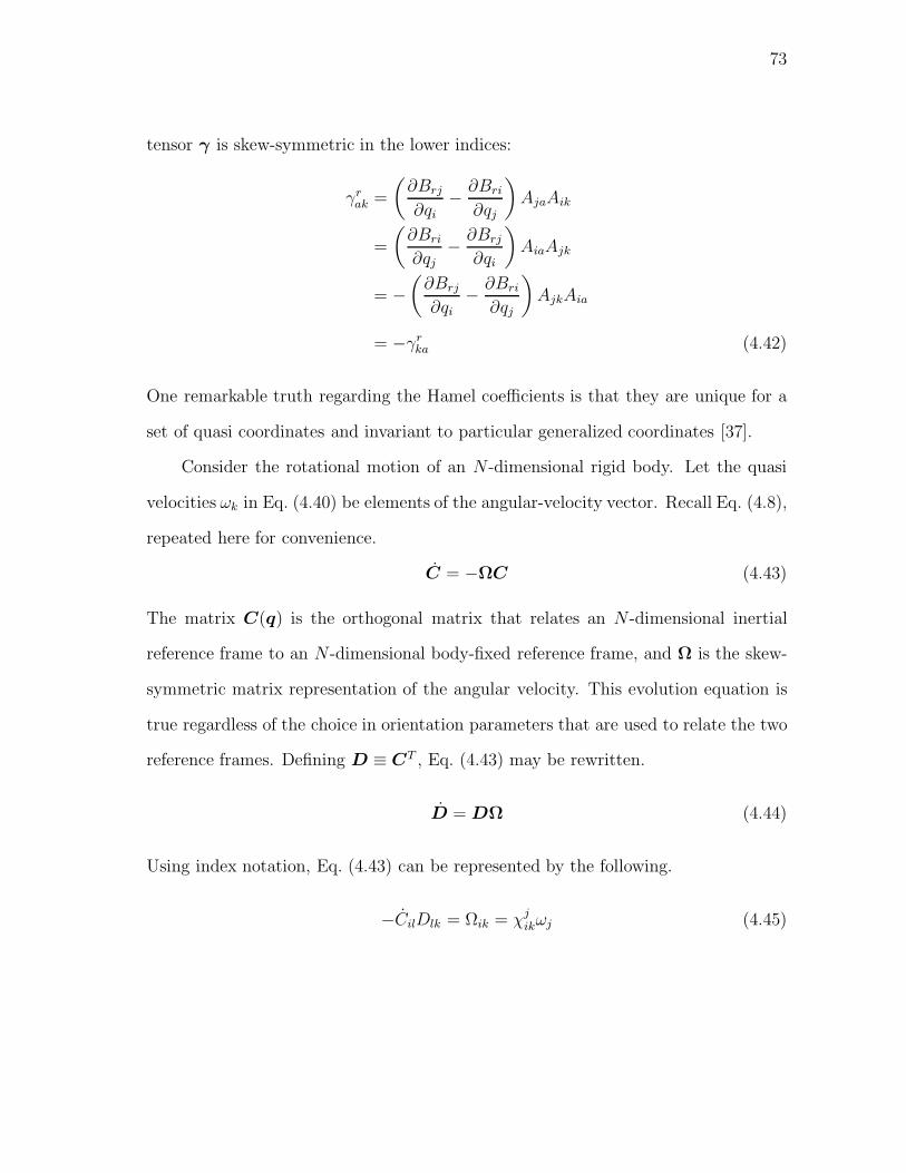
73

tensor γ is skew-symmetric in the lower indices:

γrak =

(∂Brj

∂qi

− ∂Bri

∂qj

)AjaAik

=

(∂Bri

∂qj− ∂Brj

∂qi

)AiaAjk

= −(∂Brj

∂qi− ∂Bri

∂qj

)AjkAia

= −γrka (4.42)

One remarkable truth regarding the Hamel coefficients is that they are unique for a

set of quasi coordinates and invariant to particular generalized coordinates [37].

Consider the rotational motion of an N -dimensional rigid body. Let the quasi

velocities ωk in Eq. (4.40) be elements of the angular-velocity vector. Recall Eq. (4.8),

repeated here for convenience.

C = −ΩC (4.43)

The matrix C(q) is the orthogonal matrix that relates an N -dimensional inertial

reference frame to an N -dimensional body-fixed reference frame, and Ω is the skew-

symmetric matrix representation of the angular velocity. This evolution equation is

true regardless of the choice in orientation parameters that are used to relate the two

reference frames. Defining D ≡ CT , Eq. (4.43) may be rewritten.

D = DΩ (4.44)

Using index notation, Eq. (4.43) can be represented by the following.

−CilDlk = Ωik = χjikωj (4.45)

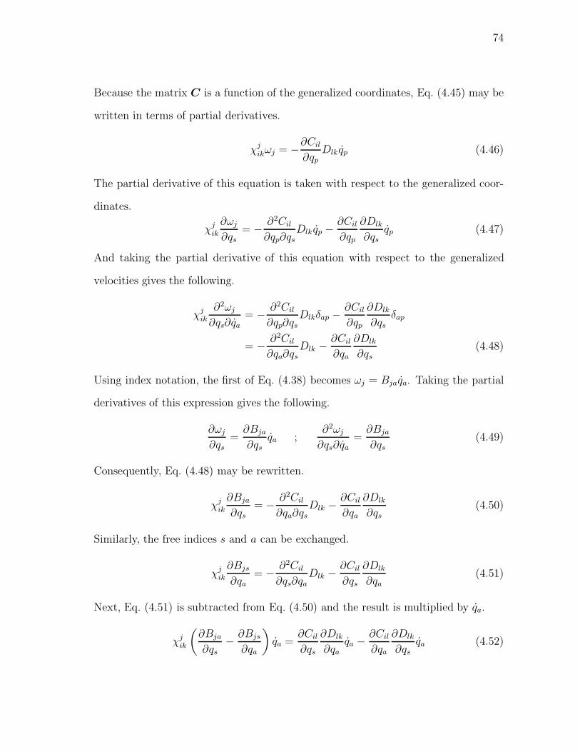
74

Because the matrix C is a function of the generalized coordinates, Eq. (4.45) may be

written in terms of partial derivatives.

χjikωj = −∂Cil

∂qpDlk qp (4.46)

The partial derivative of this equation is taken with respect to the generalized coor-

dinates.

χjik

∂ωj

∂qs= − ∂2Cil

∂qp∂qsDlk qp − ∂Cil

∂qp

∂Dlk

∂qsqp (4.47)

And taking the partial derivative of this equation with respect to the generalized

velocities gives the following.

χjik

∂2ωj

∂qs∂qa

= − ∂2Cil

∂qp∂qs

Dlkδap − ∂Cil

∂qp

∂Dlk

∂qs

δap

= − ∂2Cil

∂qa∂qsDlk − ∂Cil

∂qa

∂Dlk

∂qs(4.48)

Using index notation, the first of Eq. (4.38) becomes ωj = Bjaqa. Taking the partial

derivatives of this expression gives the following.

∂ωj

∂qs=∂Bja

∂qsqa ;

∂2ωj

∂qs∂qa=∂Bja

∂qs(4.49)

Consequently, Eq. (4.48) may be rewritten.

χjik

∂Bja

∂qs= − ∂2Cil

∂qa∂qsDlk − ∂Cil

∂qa

∂Dlk

∂qs(4.50)

Similarly, the free indices s and a can be exchanged.

χjik

∂Bjs

∂qa= − ∂2Cil

∂qs∂qaDlk − ∂Cil

∂qs

∂Dlk

∂qa(4.51)

Next, Eq. (4.51) is subtracted from Eq. (4.50) and the result is multiplied by qa.

χjik

(∂Bja

∂qs

− ∂Bjs

∂qa

)qa =

∂Cil

∂qs

∂Dlk

∂qa

qa − ∂Cil

∂qa

∂Dlk

∂qs

qa (4.52)

75

The partial derivatives in the first term on the right-hand side can be rewritten as

follows.

∂Dlk

∂qaqa = Dlk = Dlpχ

rpkωr (4.53)

Similar steps are performed on the partial derivatives from the second term on the

right-hand side.

∂Cil

∂qaqa = Cil = −χr

ipωrCpl (4.54)

These results can be substituted into Eq. (4.52).

χjik

(∂Bja

∂qs− ∂Bjs

∂qa

)qa =

∂Cil

∂qsDlpχ

rpkωr +

∂Dlk

∂qsχr

ipωrCpl (4.55)

Notice that substituting for ωr = Brsqs in Eqs. (4.53) and (4.54) gives the following.

∂Dlk

∂qs= Dlvχ

cvkBcs ;

∂Cil

∂qs= −χv

icCclBvs (4.56)

Using these expressions, Eq. (4.55) is rewritten.

χjik

(∂Bja

∂qs− ∂Bjs

∂qa

)qa = −χv

icCclBvsDlpχrpkωr +Dlvχ

cvkBcsχ

ripωrCpl (4.57)

The first term on the right-hand side may be manipulated in the following way.

−χvicCclBvsDlpχ

rpkωr = −χv

icδcpBvsχrpkωr

= −χvicBvsχ

rckωr (4.58)

The second term on the right-hand side may be manipulated in a similar manner.

DlvχcvkBcsχ

ripωrCpl = δpvχ

cvkBcsχ

ripωr

= χcvkBcsχ

rivωr

= χvckBvsχ

ricωr (4.59)

76

Using Eqs. (4.58) and (4.59) in Eq. (4.57) gives the following expression.

χjik

(∂Bja

∂qs

− ∂Bjs

∂qa

)qa = (χv

ckχric − χv

icχrck)Bvsωr (4.60)

Now note the following.

∂Bja

∂qs=∂Bja

∂qlδls ;

∂Bjs

∂qa=∂Bjl

∂qaδls (4.61)

These expressions may be used on the left-hand side of Eq. (4.60).

χjik

(∂Bja

∂ql− ∂Bjl

∂qa

)δlsqa = (χv

ckχric − χv

icχrck)Bvsωr

χjik

(∂Bja

∂ql− ∂Bjl

∂qa

)AlvBvsqa =

χjik

(∂Bja

∂ql

− ∂Bjl

∂qa

)AlvBvsAarωr = (4.62)

Using the definition of the Hamel coefficients from Eq. (4.41), and the skew-symmetry

property γjrv = −γj

vr, Eq. (4.62) is rewritten.

−χjikBvsωrγ

jvr = (χv

ckχric − χv

icχrck)Bvsωr (4.63)

The following can then be concluded.

χjikγ

jvr = χv

icχrck − χv

ckχric (4.64)

Applying Eq. (4.25) allows the following simplifications.

1

2χm

ikχjikγ

jvr =

1

2χm

ik (χvicχ

rck − χv

ckχric)

δmjγjvr =

1

2χm

ik (χvicχ

rck − χv

ckχric)

γmvr =

1

2χm

ik (χvicχ

rck − χv

ckχric) (4.65)

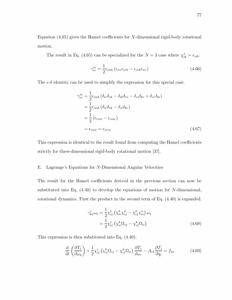
77

Equation (4.65) gives the Hamel coefficients for N -dimensional rigid-body rotational

motion.

The result in Eq. (4.65) can be specialized for the N = 3 case where χjik = εijk.

γmvr =

1

2εimk (εivcεcrk − εcvkεirc) (4.66)

The ε-δ identity can be used to simplify the expression for this special case.

γmvr =

1

2εimk (δirδvk − δikδrv − δviδkr + δvrδki)

=1

2εimk (δirδvk − δviδkr)

=1

2(εrmv − εvmr)

= εrmv = εvrm (4.67)

This expression is identical to the result found from computing the Hamel coefficients

strictly for three-dimensional rigid-body rotational motion [37].

E. Lagrange’s Equations for N -Dimensional Angular Velocities

The result for the Hamel coefficients derived in the previous section can now be

substituted into Eq. (4.40) to develop the equations of motion for N -dimensional,

rotational dynamics. First the product in the second term of Eq. (4.40) is expanded.

γrkaωa =

1

2χr

ij

(χk

icχacj − χk

cjχaic

)ωa

=1

2χr

ij

(χk

icΩcj − χkcjΩic

)(4.68)

This expression is then substituted into Eq. (4.40).

d

dt

(∂T1

∂ωk

)+

1

2χr

ij

(χk


) ∂T1

∂ωr− Ark

∂T1

∂qr= f1k (4.69)

78

Equation (4.69) is the vector form of the rotational equations of motion of N -dimen-

sional rigid bodies.

These M general equations of motion for N -dimensional space can be simplified

to the familiar form for N = 3. Returning to Eq. (4.40), the three-dimensional Hamel

coefficient found in Eq. (4.67) is substituted.

d

dt

(∂T1

∂ωk

)+ εkarωa

∂T1

∂ωr− Ark

∂T1

∂qr= f1k

d

dt

(∂T1

∂ωk

)+ Ωkr

∂T1

∂ωr− Ark

∂T1

∂qr= f1k (4.70)

As mentioned in the review of N -dimensional kinematics, for N = 3 the skew-

symmetric matrix Ω represents a cross product with the generating vector, ω. Ad-

ditionally, for the case of rotational motion of a rigid body about a fixed point the

kinetic energy can be represented by the following.

T1 =1

2Iijωiωj (4.71)

This is independent of qr, and therefore the equations of motion simplify.

d

dt

(∂T1

∂ωk

)+ Ωkr

∂T1

∂ωr= f1k (4.72)

In vector notation this leads to the familiar representation of Euler’s rotational equa-

tions of motion about a fixed point.

Iω + ω × Iω = f1 (4.73)

The vector f1 is the vector of applied torques.

79

F. The Lax Pair Form Via the Lagrangian Method

From the vector form of the N -dimensional, rotational equations of motion, a matrix

form of the N -dimensional rigid-body equations can be obtained in a straightforward

way. Substituting the matrix forms of the generalized coordinates, qi = 12χi

jkQjk, and

the angular velocity, ωi = 12χi

jkΩjk, gives a new expression for the kinetic energy:

T = T1 (Q,Ω). The equations of motion can then be simplified by using the chain

rule.

∂T1

∂Ωij=∂T1

∂ωr

∂ωr

∂Ωij=

1

2χr

ij

∂T1

∂ωr

Using the above, Eq. (4.69) is rewritten as follows.

d

dt

(∂T1

∂ωk

)+(χk


) ∂T1

∂Ωij− Ark

∂T1

∂qr= f1k (4.74)

This form is mapped into a matrix form by multiplication with χkjl.

χkjl

d

dt

(∂T1

∂ωk

)+ χk

jl

(χk

icΩcd − χkcdΩic

) ∂T1

∂Ωid= χk

jl

(f1k + Ark

∂T1

∂qr

)(4.75)

For convenience the parenthetical term on the right-hand side is defined as gk, and

the vector g is used to generate the skew-symmetric matrix G. The chain rule is

again used to rewrite the derivatives in terms of the matrix components.

2d

dt

(∂T1

∂Ωjl

)+(χk

jlχkicΩcd − χk

jlχkcdΩic

) ∂T1

∂Ωid= Gjl (4.76)

To follow convention, the partial derivative of the kinetic energy with respect to

ω is defined as the angular-momentum vector, l.

∂T1

∂ωk

= lk (4.77)

80

The partial derivative of the kinetic energy with respect to Ω is expressed using the

chain rule.

∂T1

∂ωk=

∂T1

∂Ωij

∂Ωij

∂ωk= χk

ij

∂T1

∂Ωij(4.78)

The angular-momentum vector is used to generate the angular-momentum matrix,

L.

lk =1

2χk

ijLij (4.79)

This gives the following result.

∂T1

∂Ωij=

1

2Lij (4.80)

The equations of motion can now be rewritten in terms of the angular-momentum

matrix.

2d

dt

(1

2Ljl

)+(χk

jlχkicΩcd − χk

jlχkcdΩic

) 1

2Lid = Gjl (4.81)

Next, the χ-δ identity is used.

d

dt(Ljl) + ((δjiδlc − δjcδli)Ωcd − (δjcδld − δjdδlc)Ωic)

1

2Lid = Gjl

d

dt(Ljl) +

1

2(ΩldLjd − ΩjdLld − ΩijLil + ΩilLij) = Gjl

d

dt(Ljl) + (−LjdΩdl + ΩjdLdl) = Gjl (4.82)

In matrix notation, Eq. (4.82) is written as the following, where the square

brackets represent the matrix Lie bracket [20].

L = (LΩ− ΩL) + G = [L,Ω] + G (4.83)

Due to the inverse property of χijk, an alternative path from Eq. (4.74) to

Eq. (4.83) can be taken by extracting the factor χijk instead of multiplying by χi

jk;

however, this is not shown here. Note that because of the skew-symmetry of the

angular-momentum matrix L, there are M independent, first-order differential equa-

81

tions in this N×N matrix differential equation. Although extracting the M indepen-

dent equations is straightforward, they will be functions of L and Ω, each with N2

elements. To use these equations one must also recognize that each of these matri-

ces has only M independent elements. A set of kinematic equations is also needed to

complete the motion description. Two choices are the M-dimensional vector equation

q = Aω, or M independent elements of the matrix equation C = −ΩC.

Equation (4.83) is the same Lax pair representation that is obtained using the

Hamiltonian method of mechanics [21,24,28]. This equation is the matrix form of the

generalized Euler equations. Its derivation here differs from those that are typically

reported. Typically, a path along the Hamiltonian method of mechanics is followed to

arrive at the free form (G = 0) of Eq. (4.83). This method takes a strong geometric

view of mechanics while using the principle that the time derivative of the angular

momentum of a free N -dimensional rigid body is zero. Abstract algebra is then used

to express the time derivative in an arbitrary coordinate system as shown in Eq. (4.83).

Note that G = 0 means that the Hamiltonian approach considers systems that have

kinetic-energy functions that are left-invariant (do not depend on the generalized

coordinates) and are not subject to externally applied torques. Here, Eq. (4.83) is

derived by following the Lagrangian method of mechanics. The Lagrangian method

is more focused on variational principles than on geometric structures. Also note

that the derivation of Eq. (4.83) has allowed a forcing term on the right-hand side

as well as the possibility that the kinetic-energy function depends on the generalized

coordinates.

82

G. Conclusions

To the student of three-dimensional rotational motion, many concepts are understood

through an intuition gained from experience in the three-dimensional world. Study

of N -dimensional rotations reveals which of these concepts apply to rotational mo-

tion in general and which are peculiar to three-dimensional space. In this chapter

three remarkable properties of the N = 3 special case were discussed: (1) the num-

ber of angular-velocity components is equal to N ; (2) the number of cross-product

components is equal to N ; and (3) the range of the indices of χjik is equal to the

number of indices. The first two of these properties are related and derive from the

fact that for N = 3 any vector has only one plane perpendicular to it. There is a

vector-plane equivalency in three-dimensional space. The third property, however, is

independent. It derives from the fact that, combined, a matrix and vector have three

dimensions. This itself may be an artifact of the development of linear algebra to

match our experience with N = 3.

A key to the development shown in this chapter for the equations of motion for N -

dimensional rotations was the use of Lagrange’s method. Unlike previous derivations,

the current development provides a convenient vector form of the equations, allows

the study of systems with forcing functions, and allows for the sensitivity of the kinetic

energy to the generalized coordinates. In this chapter, a useful new numerical relative

tensor was also developed that allows for the straightforward mapping between skew-

symmetric and vectorial representations of motion variables and equations.

In methods based on directly generalizing Euler’s equations it is difficult to in-

clude the concept of applied moments. Newton’s and Euler’s laws are examples of

principles based on experience with N = 3: they are empirical relationships that

have been found to model the motion of three-dimensional bodies. No one has any

83

experience upon which to base an extension of these principles to higher dimensions.

The concept of generalized forces in Lagrange’s equations, however, provide a math-

ematical way to describe these concepts even if one can not physically understand

them.

The current derivation shares a certain similarity to the previous derivations in

regard to the fact that Lagrange’s equation can be derived from Hamilton’s principle.

Therefore, by applying these equations to N -dimensional bodies it has been assumed

that Hamilton’s principle holds in the spaces that these bodies occupy. This is similar

to the Hamiltonian-based derivations that have been produced in the past. The

derivation of Lagrange’s equations themselves is based on differential geometry of the

coordinate space, whose dimension is independent of the dimension of the bodies it

describes.

84

CHAPTER V

CAYLEY KINEMATICS AND THE CAYLEY FORM OF DYNAMIC

EQUATIONS∗

A. Introduction

There have been many studies to extend the principles behind rigid-body mechanics

in three-dimensional space to principles that govern motion in higher-dimensional

spaces. Some progress has been made in extending the kinematic concepts of orien-

tation, rotation, and angular velocity [2, 5–7, 10, 12, 19], and the dynamic concepts of

inertia, momenta, and impressed forces [20–24,28].

The expression that defines the angular-velocity matrix in N -dimensional space

is Ω = −CCT [7]. The matrix C is an N ×N proper orthogonal matrix which can

represent a rotation about the origin, and the angular-velocity matrix, Ω, is an N×Nskew-symmetric matrix withM = N(N−1)/2 independent elements. The rearranged

form C = −ΩC is sometimes called Poisson’s equation. Many properties of the N -

dimensional angular-velocity matrix have been established [7], and perhaps one of

the most significant is that only in three-dimensional space can the M independent

elements of the angular-velocity matrix be considered as components of an angular-

rate vector (i.e., only in three-dimensional space does N = M) [10].

Rigid rotations in N -dimensional space take place on an invariant plane and

are related to the concept of the N -dimensional vector cross-product operation [2,

19]. A natural way to parameterize an N -dimensional rigid rotation is with the

principal rotation angle and a set of twoN -dimensional orthogonal vectors that define

∗Reprinted with permission from “Cayley kinematics and the Cayley form of dy-namic equations” by A. J. Sinclair and J. E. Hurtado, 2005. Proceedings of the RoyalSociety of London Series A, 461, 761–781. 2005 by The Royal Society.

85

the invariant (principal) plane [2, 3]. It is important to note that N -dimensional

orientation is different than N -dimensional rotation: an arbitrary orientation in N -

dimensional space is a product of a minimum set of rigid rotations and only for the

N = 3 case can an arbitrary orientation be realized with one rigid rotation.

The Cayley transform and the Cayley-transform kinematic relationship are an-

other set of results that have relevance in N -dimensional orientations and rotations.

These important results have a direct bearing on this chapter and will be discussed

more fully later.

The governing equations of motion for N -dimensional rigid bodies are often pre-

sented in a matrix form. The traditional approach to deriving the equations has been

the Hamiltonian method of mechanics [20, 21, 24]. That method takes a geometric

view and uses concepts in abstract algebra and coordinate-free differential forms to

arrive at the matrix Lax pair representation of the N -dimensional generalized Euler

equations. The focus in many of these studies has been on different representations

of the equations and their integrability [24, 26–28]. Consequently, the systems that

have been addressed are those that are not subject to externally applied torques and

do not have kinetic-energy functions that depend on the generalized coordinates. In

some earlier work the vector form of the N -dimensional generalized Euler equations

was developed by using the Lagrangian method of mechanics [15]. This vector form

is easily mapped into the matrix Lax pair form. The vector form of the equations

was developed without any a priori selection of orientation parameters for the N -

dimensional rigid body.

Here an N -dimensional rigid body will be defined as a system whose configuration

can be completely defined by an N×N proper orthogonal matrix. It will be seen that

a wide variety of mechanical systems can be modeled as N -dimensional rigid bodies

using this definition, which relaxes some conditions used in earlier work. In this

86

current chapter, the Lax pair form of the N -dimensional generalized Euler equations

of motion are developed following an a priori decision to describe the system using the

Cayley orientation and kinematic variables. The Cayley orientation and kinematic

variables are then used to relate the motion of general mechanical systems to the

motion of higher-dimensional rigid bodies.

B. Cayley Kinematics

Some of the most important and elegant concepts in N -dimensional kinematics re-

late to the Cayley transform. This famous relationship provides a unique mapping

between proper orthogonal and skew-symmetric matrices [7].

C = (I −Q) (I + Q)−1 = (I + Q)−1 (I − Q) (5.1)

Q = (I −C) (I + C)−1 = (I + C)−1 (I −C) (5.2)

Here, C is an N × N proper orthogonal matrix, whereas Q is an N × N skew-

symmetric matrix. The elements of Q are an M-dimensional set of parameters that

represent N -dimensional attitude. In fact q, the generating vector of Q, is the vector

of extended Rodrigues parameters for N -dimensional spaces [5, 6].

In this section, the Cayley transform and the Cayley-transform kinematic rela-

tionship will be used to find a general expression for the extended Rodrigues parameter

rates, q, in terms of the angular-velocity vector, ω. In the derivations that follow, it

will be convenient to make the following designations.

I + Q ≡ A+ ; I − Q ≡ A− (5.3)

(I + Q)−1 ≡ B+ ; (I − Q)−1 ≡ B− (5.4)

87

The Cayley-transform kinematic relationships connect the derivatives of the M

independent parameters of Q to the angular-velocity matrix [12].

Ω = 2 (I + Q)−1 Q (I − Q)−1 = 2B+QB− (5.5)

Q =1

2(I + Q)Ω (I − Q) =

1

2A+ΩA− (5.6)

Equations (5.5) and (5.6) represent a linear mapping between the generalized veloci-

ties, Q, and a set of quasi velocities, Ω, for N -dimensional rotations. Whereas these

equations are represented as linear transformations of N ×N , skew-symmetric matri-

ces, they can be rewritten in the familiar form in terms of the linear transformation

of an M-dimensional vector. In index notation Eq. (5.6) is written as follows.

Qvp =1

2A+

vkΩklA−lp (5.7)

The generalized-velocity and angular-velocity matrices are mapped into their vector

forms using χijk.

χjvpqj =

1

2A+

vkχmklωmA

−lp (5.8)

Both sides of the above equation are multiplied by χivp.

χivpχ

jvpqj =

1

2χi

vpA+vkχ

mklωmA

−lp (5.9)

2δij qj =1

2χi

vpχmklA

+vkA

−lpωm (5.10)

qi =1

4χi

vpχmklA

+vkA

−lpωm ≡ Aimωm (5.11)

The two-index variable Aim represents the components of the matrix A that performs

a linear mapping of the angular-velocity vector onto the generalized-velocity vector.

Similarly, an expression can be found for the matrix B that performs the inverse

mapping; however, this matrix is a function of B+ and B− and thus less convenient

88

to evaluate. The expression for Aim can be expanded using the definitions of A+ and

A−.

Aim =1

4χi

vpχmklA

+vkA

−lp

=1

4χi

vpχmkl (δvk +Qvk) (δlp −Qlp)

=1

4χi

vpχmkl (δvkδlp − δvkQlp + δlpQvk −QvkQlp) (5.12)

This expression can be simplified by analyzing the first three terms.

1

4χi

vpχmklδvkδlp =

1

4χi

vpχmvp =

1

2δim (5.13)

−1

4χi

vpχmklδvkQlp = −1

4χi

vpχmvlQlp (5.14)

1

4χi

vpχmklδlpQvk =

1

4χi

vpχmkpQvk =

1

4χi

pvχmlvQpl = −1

4χi

vpχmvlQlp (5.15)

These are substituted back into Eq. (5.12) to give the final result.

Aim =1

2

(δim − χi

vpχmvlQlp − 1

2χi

vpχmklQvkQlp

)(5.16)

For the special case N = 3, the equation for the elements of A can be simplified

by substituting εijk for χjik.

Aim =1

2

(δim − εvipεvmlQlp − 1

2εvipεkmlQvkQlp

)(5.17)

The ‘ε-δ identity’ can be applied to the second term of this equation. Additionally,

the fact that Qii equals zero, because Q is skew-symmetric, is used.

εvipεvmlQlp = (δimδpl − δilδpm)Qlp = −Qim (5.18)

89

The third term of Eq. (5.17) can also be rewritten using the generalized Kronecker

delta [32].

εvipεkml = δkmlvip =

∣∣∣∣∣∣∣∣∣∣δkv δk

i δkp

δmv δm

i δmp

δlv δl

i δlp

∣∣∣∣∣∣∣∣∣∣(5.19)

= δvk (δimδpl − δpmδil) + δik (δpmδvl − δvmδpl) + δpk (δvmδil − δimδvl)

= δvkδimδpl − δvkδpmδil + δikδpmδvl − δikδvmδpl + δpkδvmδil − δpkδimδvl

The third term of Eq. (5.17) therefore becomes the following.

εvipεkmlQvkQlp = QviQvm +QmpQip − δimQvpQvp

= 2QviQvm − δimQvpQvp (5.20)

This expression is now rewritten in terms of the generating vector elements qj and

the ε-δ identity is used once again.

εvipεkmlQvkQlp = 2εvriqrεvsmqs − δimεvrpqrεvspqs

= 2 (δrsδim − δrmδis) qrqs − δim (δrsδpp − δrpδsp) qrqs

= 2δimqrqr − 2qiqm − 3δimqrqr + δimqpqp

= −2qiqm (5.21)

Equations (5.18) and (5.21) are now substituted into Eq. (5.17) to give the familiar

form for the mapping from the angular velocity to the Rodrigues parameter rates [38].

Aim =1

2(δim +Qim + qiqm) (5.22)

90

For reference, the complete form of A is given below for three- and four-dimen-

sional bodies.

[A]M=3 =1

2

⎡⎢⎢⎢⎢⎣1 + q2

1 q1q2 − q3 q1q3 + q2

q2q1 + q3 1 + q22 q2q3 − q1

q3q1 − q2 q3q2 + q1 1 + q23

⎤⎥⎥⎥⎥⎦ (5.23)

[A]M=6 =1

2

⎡⎢⎢⎢⎢⎢⎢⎢⎢⎢⎢⎢⎢⎢⎢⎣

1 + q21 q1q2 − q3 q1q3 + q2

q2q1 + q3 1 + q22 q2q3 − q1

q3q1 − q2 q3q2 + q1 1 + q23

q4q1 + q5 q4q2 + q6 q5q2 − q1q6

q5q1 − q4 q3q4 + q1q6 q5q3 + q6

q2q5 − q3q4 q6q2 − q4 q6q3 − q5

q1q4 − q5 q1q5 + q4 q2q5 − q3q4

q2q4 − q6 q3q4 + q1q6 q2q6 + q4

q2q5 − q1q6 q3q5 − q6 q3q6 + q5

1 + q24 q4q5 − q1 q4q6 − q2

q5q4 + q1 1 + q25 q5q6 − q3

q6q4 + q2 q6q5 + q3 1 + q26

⎤⎥⎥⎥⎥⎥⎥⎥⎥⎥⎥⎥⎥⎥⎥⎦(5.24)

It is noteworthy that many researchers reference Cayley’s work ‘On the Motion

of Rotation of a Solid Body’ [39] as the origin of the Cayley transform, Eqs. (5.1) and

(5.2). That paper contains scalar expressions for the case N = 3 which are equivalent

to the Cayley transform (p. 225) and the Cayley-transform kinematic relationship (p.

227). There is no indication, however, that the results apply, nor lead, to the general

N -dimensional case, nor is there any indication of the elegant, matrix forms that are

central to the Cayley transform and kinematic relationship that are recognized today.

91

To the current authors’ knowledge, these features first appear in Cayley’s work

‘Sur quelques proprietes des determinants gauches’ [8]. For reasons that are not

mentioned in that paper, Cayley investigates some properties of what he calls ‘left

systems’. A left system is defined as a square collection of quantities, λij , that satisfy

the following relationships.

λij = −λji, i = j ; λii = 1, no sum on i (5.25)

The indices i and j range from 1 to N . Note that the quantities λij are essentially

the elements of an N ×N matrix, λ, which may be expressed as λ = I − Q, where

Q is a skew-symmetric matrix. He goes on to introduce the ‘inverse left system,’ Λ,

which satisfies λT Λ = KI, where K is the determinant of λ. While investigating

some transformation properties of left systems, Cayley discovers his famous transform

(bottom of p. 120):

‘On a donc le theoreme suivant: Les coefficients propres a la transfor-

mation de coordonnees rectangulaires, peuvent etre exprimes rationnelle-

ment au moyen de quantites arbitraires λrs, soumises aux conditions

λrs = −λsr , [r = s]; λrr = 1. Pour les developper, il faut d’abord for-

mer le determinant K de ce systeme, puis le systeme inverse Λrs, . . . et

ecrire Kαrs = 2Λrs [r = s]; Kαrr = 2Λrr − K; ce qui donne le systeme

cherche.’

Cayley’s coefficients αrs are equivalent to the elements of C, and the relationship in

Cayley’s theorem can be writtenKC = 2Λ−KI. Using λT Λ = KI, the relationship

is seen to become KC = λΛ. When λ is written as λ = I − Q, the inverse system

is Λ = K(I + Q)−1, which leads to C = (I − Q)(I + Q)−1. From this result, it

is straightforward to write the inverse form of the Cayley transform relating skew-

92

symmetric Q to the proper orthogonal matrix C. Note that although Cayley does not

use matrix notation, he does use what is recognized today as a form of index notation

to manipulate system quantities (i.e., matrix elements). A generalization of the Cay-

ley transform in matrix notation appears in Cayley’s works ‘Sur la transformation

d’une fonction quadratique en elle meme par des substitutions lineaires’ (p. 288) [40]

and ‘A Memoir on the Automorphic Linear Transformation of a Bipartite Quadric

Function’ (p. 44) [41]. These papers consider the transformation of the variables of

quadratic functions and not just the rotation of an orthogonal coordinate system.

In the following section, the Cayley kinematics are used (as generalized coordinates

and motion variables) to directly derive the equations for rotational motion of an

N -dimensional body.

C. Tensor Form of Lagrange’s Equations

Previously, the tensor form of the N -dimensional rotational equations of motion have

been derived by generalizing Euler’s equations via a Hamiltonian approach [21,24,28]

or by mapping the vector form of Lagrange’s equations in terms of the Hamel coef-

ficients [15]. In this section a new approach is presented using Lagrange’s equations

and Cayley kinematics to directly derive the tensor form of the equations of motion.

Lagrange’s equations of motion in terms of the generalized coordinates and ve-

locities are given by the following familiar form.

d

dt

(∂T0

∂qi

)− ∂T0

∂qi= fi (5.26)

In this equation T0 = T0 (q, q) is a function of the generalized-coordinate and velocity

vectors and is equal to the kinetic energy of the system. The generalized forces, fi,

are associated with the generalized coordinates.

93

This equation can be rewritten in terms of the generalized-coordinate and velocity

matrices. To do this the skew-symmetric matrix elements are substituted using the

relationships given below.

qi =1

2χi

jkQjk ; qi =1

2χi

jkQjk (5.27)

Substituting Eqs. (5.27) into the expression for T0 for any given system will define

a new kinetic-energy function T0 = T0(Q, Q). Whereas Eqs. (5.27) give the vector

elements in terms of the matrix elements, the inverse mapping can also be considered.

Qjk = χljkql ; Qjk = χl

jkql (5.28)

The partial derivatives of these equations can be used to find a matrix form of La-

grange’s equations.

∂Qjk

∂qi

= χljk

∂ql

∂qi

= χljkδli = χi

jk (5.29)

∂Qjk

∂qi= χl

jk

∂ql

∂qi= χl

jkδli = χijk (5.30)

Although the elements of Q, Q, and Ω satisfy the skew-symmetry constraint, in

the following derivations one has the choice of enforcing the constraint or not. Either

option will produce the correct, final equation of motion as long as it is applied

consistently (see Appendix B). For convenience, the constraint is not enforced in the

following derivations, and in essence, the elements of these skew-symmetric matrices

are treated as independent. This allows the partial derivatives of the kinetic-energy

function with respect to the matrix elements to be written using the following chain

rules without a priori considering the form of the constraint.

∂T0

∂qi=

∂T0

∂Qjk

∂Qjk

∂qi= χi

jk

∂T0

∂Qjk(5.31)

94

∂T0

∂qi

=∂T0

∂Qjk

∂Qjk

∂qi

= χijk

∂T0

∂Qjk

(5.32)

Substituting these expressions into Lagrange’s equations gives the following.

d

dt

(χi

jk

∂T0

∂Qjk

)− χi

jk

∂T0

∂Qjk

= fi (5.33)

χijk

d

dt

(∂T0

∂Qjk

)− ∂T0

∂Qjk

=

1

2χi

jkFjk (5.34)

d

dt

(∂T0

∂Qij

)− ∂T0

∂Qij

=1

2Fij (5.35)

Here, F represents the skew-symmetric matrix of generalized forces. Equation (5.35)

is the matrix form of Lagrange’s equations in terms of the generalized coordinates

and velocities. The factor of one-half appears on the right-hand side because the

contribution to T0 due to the generalized coordinate qi (or the generalized velocity

qi) is shared in T0 equally between the corresponding Qjk and Qkj (or Qjk and Qkj)

elements.

The matrix form of Lagrange’s equations in terms of generalized coordinates and

quasi velocities will now be developed. To do this another kinetic-energy function,

T1 = T1 (Q,Ω), is defined by substituting the Cayley-transform kinematic relation-

ship into T0. The partial derivatives of T0 can be expressed in terms of T1 by using

the chain rule.

∂T0

∂Qij=

∂T1

∂Qij+

∂T1

∂Ωkl

∂Ωkl

∂Qij(5.36)

∂T0

∂Qij

=∂T1

∂Ωkl

∂Ωkl

∂Qij

(5.37)

These expansions are substituted into Eq. (5.35).

d

dt

(∂T1

∂Ωkl

∂Ωkl

∂Qij

)−(∂T1

∂Qij+∂T1

∂Ωkl

∂Ωkl

∂Qij

)=

1

2Fij (5.38)

95

d

dt

(∂T1

∂Ωkl

∂Ωkl

∂Qij

)− ∂T1

∂Ωkl

∂Ωkl

∂Qij

=1

2Fij +

∂T1

∂Qij

(5.39)

In order to expand the terms on the left-hand side of this equation, the derivatives

of the elements of Ω must be considered. Thus, Eq. (5.5) is rewritten in index

notation.

Ωkl = 2B+kvQvpB

−pl (5.40)

In order to develop the first term of Eq. (5.39) the derivative of Ωkl with respect

to Qij is considered.

∂Ωkl

∂Qij

= 2B+kv

∂Qvp

∂Qij

B−pl = 2B+

kvδivδjpB−pl = 2B+

kiB−jl (5.41)

The first term of Eq. (5.39) is therefore given by the following.

d

dt

(∂T1

∂Ωkl

∂Ωkl

∂Qij

)=

d

dt

(2∂T1

∂ΩklB+

kiB−jl

)

= 2d

dt

(∂T1

∂Ωkl

)B+

kiB−jl + 2

∂T1

∂Ωkl

(B+

kiB−jl +B+

kiB−jl

)(5.42)

Clearly the matrices B+ and B− must be investigated. These are found using

the definitions in Eqs. (5.3) and (5.4).

A+B+ = I (5.43)

Taking a derivative gives the following.

A+B+ + A+B+ = 0 (5.44)

B+ = −B+A+B+ (5.45)

From the definition of A+, however, it is true that A+ = Q.

B+ = −B+QB+ (5.46)

96

By applying similar steps to the product A−B−, the derivative of B− can be found.

B− = B−QB− (5.47)

These expressions for B+ and B− are substituted back into Eq. (5.42).

d

dt

(∂T1

∂Ωkl

∂Ωkl

∂Qij

)=2

d

dt

(∂T1

∂Ωkl

)B+

kiB−jl (5.48)

+ 2∂T1

∂Ωkl

(−B+

krQrsB+siB

−jl +B+

kiB−jrQrsB

−sl

)Now the second term of Eq. (5.39) is considered. First, the derivative of Ωkl with

respect to Qij is given by the following.

∂Ωkl

∂Qij= 2

∂B+kv

∂QijQvpB

−pl + 2B+

kvQvp

∂B−pl

∂Qij(5.49)

This result is used to rewrite the second term of Eq. (5.39).

∂T1

∂Ωkl

∂Ωkl

∂Qij= 2

∂T1

∂Ωkl

(∂B+

kv

∂QijQvpB

−pl +B+

kvQvp

∂B−pl

∂Qij

)(5.50)

The derivatives of B+ and B− with respect to the elements of Q must be inves-

tigated.

A+rkB

+kv = δrv (5.51)

∂A+rk

∂QijB+

kv + A+rk

∂B+kv

∂Qij= 0 (5.52)

∂B+sv

∂Qij= −B+

sr

∂A+rk

∂QijB+

kv (5.53)

The derivatives of A+rk can be found using the definition of A+.

∂A+rk

∂Qij=∂Qrk

∂Qij= δirδjk (5.54)

97

Based on this, the derivative of B+sv is given by the following.

∂B+sv

∂Qij

= −B+srδirδjkB

+kv = B+

siB+jv (5.55)

By applying similar steps to B− the derivatives of its elements are found.

∂B−sv

∂Qij= B−

siB−jv (5.56)

Substituting Eqs. (5.55) and (5.56) into Eq. (5.50) gives the following for the second

term of Eq. (5.39).

∂T1

∂Ωkl

∂Ωkl

∂Qij= 2

∂T1

∂Ωkl

(−B+

kiB+jvQvpB

−pl +B+

kvQvpB−piB

−jl

)(5.57)

Finally, Eqs. (5.48) and (5.57) can be substituted back into Eq. (5.39).

2d

dt

(∂T1

∂Ωkl

)B+

kiB−jl + 2

∂T1

∂Ωkl

(−B+

krQrsB+siB

−jl +B+

kiB−jrQrsB

−sl

)− 2

∂T1

∂Ωkl

(−B+

kiB+jvQvpB

−pl +B+

kvQvpB−piB

−jl

)=

1

2Fij +

∂T1

∂Qij(5.58)

The second and third terms of the left-hand side can be grouped.

2d

dt

(∂T1

∂Ωkl

)B+

kiB−jl+2

∂T1

∂ΩklQrs

(−B+krB

+siB

−jl +B+

kiB−jrB

−sl

+B+kiB

+jrB

−sl − B+

krB−siB

−jl

)=

1

2Fij +

∂T1

∂Qij(5.59)

2d

dt

(∂T1

∂Ωkl

)B+

kiB−jl + 2

∂T1

∂ΩklQsr

(−B+ksB

+riB

−jl +B+

kiB−jsB

−rl

+B+kiB

+jsB

−rl −B+

ksB−riB

−jl

)=

1

2Fij +

∂T1

∂Qij(5.60)

98

2d

dt

(∂T1

∂Ωkl

)B+

kiB−jl +

∂T1

∂Ωkl

A+saΩabA

−br

(B+

kiB−rl

(B−

js +B+js

)−B+

ksB−jl

(B+

ri +B−ri

))=

1

2Fij +

∂T1

∂Qij

(5.61)

Both sides of the above equation are now multiplied by A+idA

−cj to allow for future

simplifications.

2d

dt

(∂T1

∂Ωkl

)B+

kiB−jlA

+idA

−cj + Ωab

∂T1

∂ΩklA+

idA−cjA

+saA

−br

(B+

kiB−rl

(B−

js +B+js

)−B+

ksB−jl

(B+

ri +B−ri

))=

(1

2Fij +

∂T1

∂Qij

)A+

idA−cj (5.62)

Both terms on the left-hand side of the above equation can be simplified. It is

convenient to start with the first term.

B+kiB

−jlA

+idA

−cj = δkdδcl (5.63)

This result is used to rewrite the first term of Eq. (5.62).

2d

dt

(∂T1

∂Ωkl

)B+

kiB−jlA

+idA

−cj = 2δkdδcl

d

dt

(∂T1

∂Ωkl

)

= 2d

dt

(∂T1

∂Ωdc

)(5.64)

The second term of Eq. (5.62) is now examined.

A+idA

−cjA

+saA

−br

(B+

kiB−rl

(B−

js +B+js

)− B+ksB

−jl

(B+

ri +B−ri

))= A+

saA−br

(δkdA

−cjB

−rl

(B−

js +B+js

)− δclA+idB

+ks

(B+

ri +B−ri

))= A+

saA−br

(δkdB

−rl (δcs + Ccs) − δclB

+ks (δdr + Cdr)

)(5.65)

99

The elements of C + I can be found using the Cayley transform.

C + I = (I − Q) (I + Q)−1 + I

= (I + Q)−1 −Q (I + Q)−1 + I

= (I + Q)−1 −Q (I + Q)

−1+ (I + Q) (I + Q)

−1

= 2 (I + Q)−1

= 2B+ (5.66)

This result can be used to further simplify Eq. (5.65).

A+idA

−cjA

+saA

−br

(B+

kiB−rl

(B−

js +B+js

)− B+ksB

−jl

(B+

ri +B−ri

))= A+

saA−br

(2δkdB

−rlB

+cs − 2δclB

+ksB

+dr

)= 2A+

saA−br

(δkdB

−rlB

+cs − δclB

−skB

+dr

)(5.67)

This result is used to rewrite the second term of Eq. (5.62).

Ωab∂T1

∂ΩklA+

idA−cjA

+saA

−br

(B+

kiB−rl

(B−

js +B+js

)− B+ksB

−jl

(B+

ri +B−ri

))= 2Ωab

∂T1

∂ΩklA+

saA−br

(δkdB

−rlB

+cs − δclB

−skB

+dr

)(5.68)

The skew-symmetry of Ω is used in the following manner.

− ∂T1

∂ΩklδclB

−skB

+dr =

∂T1

∂ΩlkδclB

−skB

+dr

=∂T1

∂Ωkl

δckB−slB

+dr (5.69)

100

This expression is substituted into Eq. (5.68).

Ωab∂T1

∂Ωkl

A+idA

−cjA

+saA

−br

(B+

kiB−rl

(B−

js +B+js

)− B+ksB

−jl

(B+

ri +B−ri

))= 2Ωab

∂T1

∂ΩklA+

saA−br

(δkdB

−rlB

+cs + δckB

−slB

+dr

)= 2Ωab

∂T1

∂Ωkl

(δkdδcaδbl + δckδlaδbd)

= 2Ωcl∂T1

∂Ωdl+ 2Ωld

∂T1

∂Ωcl

= 2∂T1

∂Ωdl

Ωcl − 2∂T1

∂Ωcl

Ωdl (5.70)

Equations (5.64) and (5.70) can now be substituted back into Eq. (5.62).

d

dt

(∂T1

∂Ωdc

)+∂T1

∂Ωdl

Ωcl − ∂T1

∂Ωcl

Ωdl =1

2

(1

2Fij +

∂T1

∂Qij

)A+

idA−cj (5.71)

The above equation is the matrix form of Lagrange’s equations for generalized co-

ordinates and the N ×N angular-velocity matrix (or Cayley quasi velocity matrix).

For convenience the right-hand side is defined as 12Gdc, where G is related to the

generating vector g whose elements can be shown to be gk = Ark (fr + ∂T1/∂qr). The

equivalent vector representation of the equations is the following.

d

dt

(∂T1

∂ωk

)+

1

2χr

ij

(χk


)(∂T1

∂ωr

)= gk (5.72)

To express these equations in the Lax pair form, the derivative of T1 with respect to

the angular-velocity components is defined as the angular-momentum vector l.

∂T1

∂ωk

= lk (5.73)

The partial derivative of the kinetic energy with respect to Ω is expressed using the

chain rule.

∂T1

∂ωk=

∂T1

∂Ωij

∂Ωij

∂ωk= χk

ij

∂T1

∂Ωij(5.74)

101

The angular-momentum vector is used to generate the angular-momentum matrix L.

lk =1

2χk

ijLij (5.75)

This gives the following result.

∂T1

∂Ωij

=1

2Lij (5.76)

Equation (5.71) can now be rewritten in terms of the angular-momentum matrix.

d

dt

(1

2Ldc

)+

1

2LdlΩcl − 1

2LclΩdl =

1

2Gdc (5.77)

In matrix notation this result gives the following Lax pair form.

L = (LΩ− ΩL) + G = [L,Ω] + G (5.78)

D. Cayley Quasi Velocities and the Cayley Form

An M-degree-of-freedom (DOF) mechanical system can be intimately related to an

N -dimensional rigid body through the Cayley kinematic equations. Recall the Cayley

kinematic equations.

Forward relationship: Ω = 2(I + Q)−1 Q (I − Q)−1 (5.79)

Inverse relationship: Q =1

2(I + Q)Ω (I −Q) (5.80)

And recall also the forward Cayley transform expression and Poisson’s equation for

C .

Forward relationship: C = (I −Q)(I + Q)−1 = (I + Q)−1(I − Q) (5.81)

Poisson’s equation: C = −ΩC (5.82)

102

These lead to the following remarkable result:

If the M-dimensional (M = N(N − 1)/2) generalized-coordinate vector,

q, of an M-DOF mechanical system is considered the generating vector of

an N ×N skew-symmetric matrix Q, and if Q and its derivative are used

to define the quasi velocities Ω via the forward Cayley kinematic equation,

then Q generates a proper N ×N orthogonal matrix, C, via the forward

Cayley transform that evolves according to C = −ΩC. Furthermore,

the motion of the system is governed by the following matrix differential

equations.

Q =1

2(I + Q)Ω (I −Q) ; L = [L,Ω] + G

Consequently, the motion of an M-DOF mechanical system can be viewed

as the rotational motion of an N -dimensional rigid body. When q is

used in this manner (i.e., a generating vector), its elements are called

the extended Rodrigues parameters; the elements of Ω are given the name

Cayley quasi velocities; and this treatment is called the Cayley Form.

The equivalent body is defined as an N -dimensional rigid body because the

generalized coordinates that define the extended Rodrigues parameters completely

describe the configuration of the system. This is an extension of the kinematic def-

inition of a three-dimensional rigid body. Previous researchers have also extended

certain dynamic properties relating to three-dimensional rigid bodies in their defini-

tions of an N -dimensional rigid body [21,24,28]. These definitions, however, preclude

the study of systems whose Lagrangian functions depend on the generalized coordi-

nates. The governing equations presented herein for an M-DOF mechanical system

or, equivalently, an N -dimensional rigid body are summarized in Table IV. The nu-

103

Table IV. THE CAYLEY FORM OF DYNAMIC EQUATIONS

M-dimensional vector forms

kinematics qi = Aijωj

dynamics d(∂T1/∂ωk)/dt+ 12χr

ij

(χk


)(∂T1/∂ωr) = gk

N ×N matrix forms

kinematics Q = 12(I + Q)Ω (I − Q)

dynamics L = [L,Ω] + G

merical relative tensor χkjl can be used to map the equations from one form to the

other.

One application of the Cayley form is the representation of the general motion

of an N -dimensional body as the pure rotation of an (N + 1)-dimensional body. The

general motion of an N -dimensional body consists of M rotational and N translational

degrees of freedom.

M +N =1

2N (N − 1) +N

=1

2(N + 1)N

=1

2(N + 1) ((N + 1) − 1) (5.83)

This total number of degrees of freedom is therefore equal to the number of rotational

degrees of freedom for an (N + 1)-dimensional body, and the Cayley form can be used

to relate these two motions. In the following section the general motion of a two-

dimensional body and pure rotations of an equivalent three-dimensional body are

presented in detail.

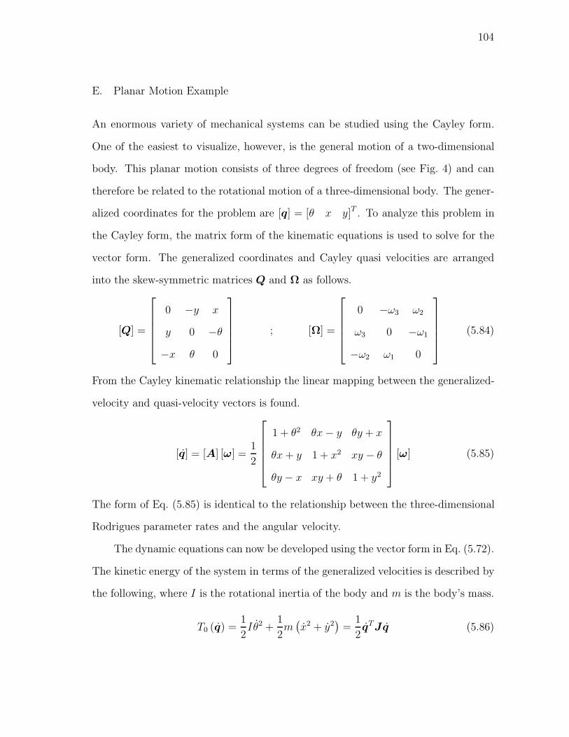
104

E. Planar Motion Example

An enormous variety of mechanical systems can be studied using the Cayley form.

One of the easiest to visualize, however, is the general motion of a two-dimensional

body. This planar motion consists of three degrees of freedom (see Fig. 4) and can

therefore be related to the rotational motion of a three-dimensional body. The gener-

alized coordinates for the problem are [q] = [θ x y]T . To analyze this problem in

the Cayley form, the matrix form of the kinematic equations is used to solve for the

vector form. The generalized coordinates and Cayley quasi velocities are arranged

into the skew-symmetric matrices Q and Ω as follows.

[Q] =

⎡⎢⎢⎢⎢⎣0 −y x

y 0 −θ−x θ 0

⎤⎥⎥⎥⎥⎦ ; [Ω] =

⎡⎢⎢⎢⎢⎣0 −ω3 ω2

ω3 0 −ω1

−ω2 ω1 0

⎤⎥⎥⎥⎥⎦ (5.84)

From the Cayley kinematic relationship the linear mapping between the generalized-

velocity and quasi-velocity vectors is found.

[q] = [A] [ω] =1

2

⎡⎢⎢⎢⎢⎣1 + θ2 θx− y θy + x

θx+ y 1 + x2 xy − θ

θy − x xy + θ 1 + y2

⎤⎥⎥⎥⎥⎦ [ω] (5.85)

The form of Eq. (5.85) is identical to the relationship between the three-dimensional

Rodrigues parameter rates and the angular velocity.

The dynamic equations can now be developed using the vector form in Eq. (5.72).

The kinetic energy of the system in terms of the generalized velocities is described by

the following, where I is the rotational inertia of the body and m is the body’s mass.

T0 (q) =1

2Iθ2 +

1

2m(x2 + y2

)=

1

2qTJq (5.86)

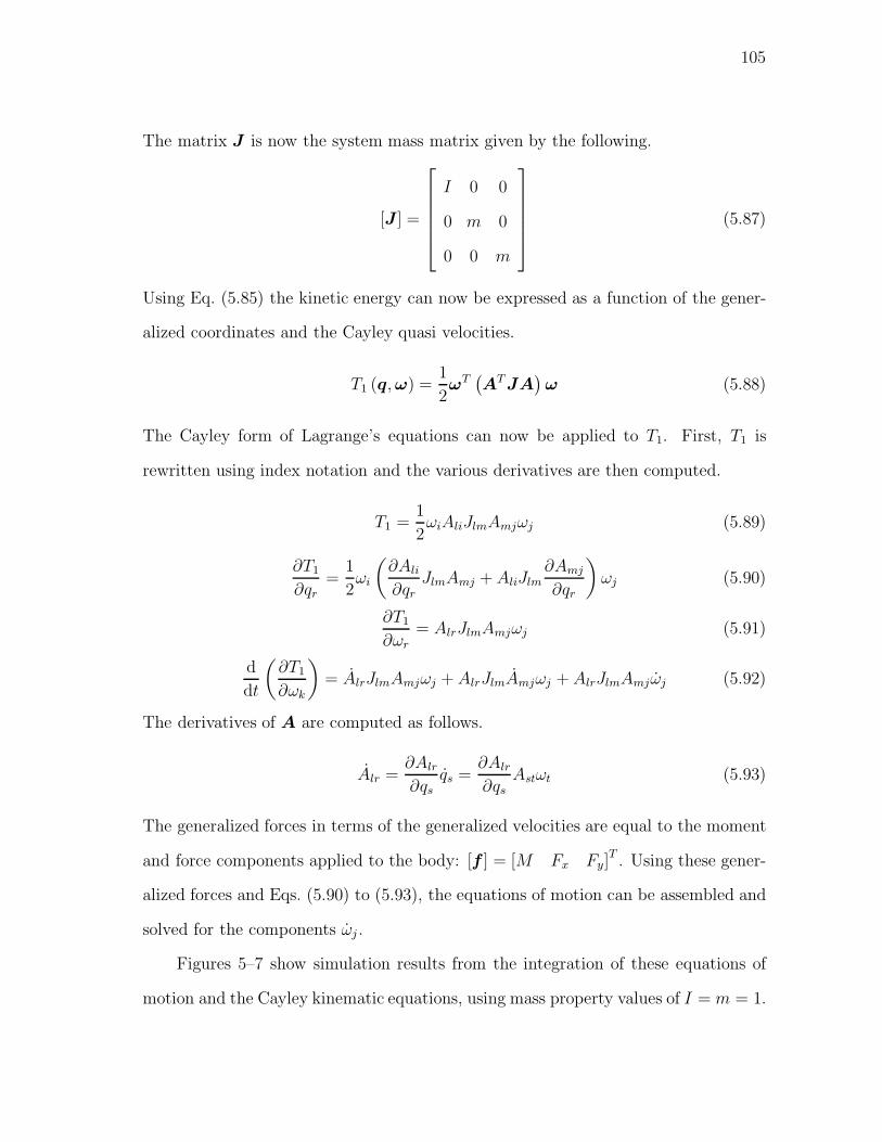
105

The matrix J is now the system mass matrix given by the following.

[J ] =

⎡⎢⎢⎢⎢⎣I 0 0

0 m 0

0 0 m

⎤⎥⎥⎥⎥⎦ (5.87)

Using Eq. (5.85) the kinetic energy can now be expressed as a function of the gener-

alized coordinates and the Cayley quasi velocities.

T1 (q,ω) =1

2ωT(AT JA

)ω (5.88)

The Cayley form of Lagrange’s equations can now be applied to T1. First, T1 is

rewritten using index notation and the various derivatives are then computed.

T1 =1

2ωiAliJlmAmjωj (5.89)

∂T1

∂qr=

1

2ωi

(∂Ali

∂qrJlmAmj + AliJlm

∂Amj

∂qr

)ωj (5.90)

∂T1

∂ωr

= AlrJlmAmjωj (5.91)

d

dt

(∂T1

∂ωk

)= AlrJlmAmjωj + AlrJlmAmjωj + AlrJlmAmjωj (5.92)

The derivatives of A are computed as follows.

Alr =∂Alr

∂qsqs =

∂Alr

∂qsAstωt (5.93)

The generalized forces in terms of the generalized velocities are equal to the moment

and force components applied to the body: [f ] = [M Fx Fy]T. Using these gener-

alized forces and Eqs. (5.90) to (5.93), the equations of motion can be assembled and

solved for the components ωj .

Figures 5–7 show simulation results from the integration of these equations of

motion and the Cayley kinematic equations, using mass property values of I = m = 1.

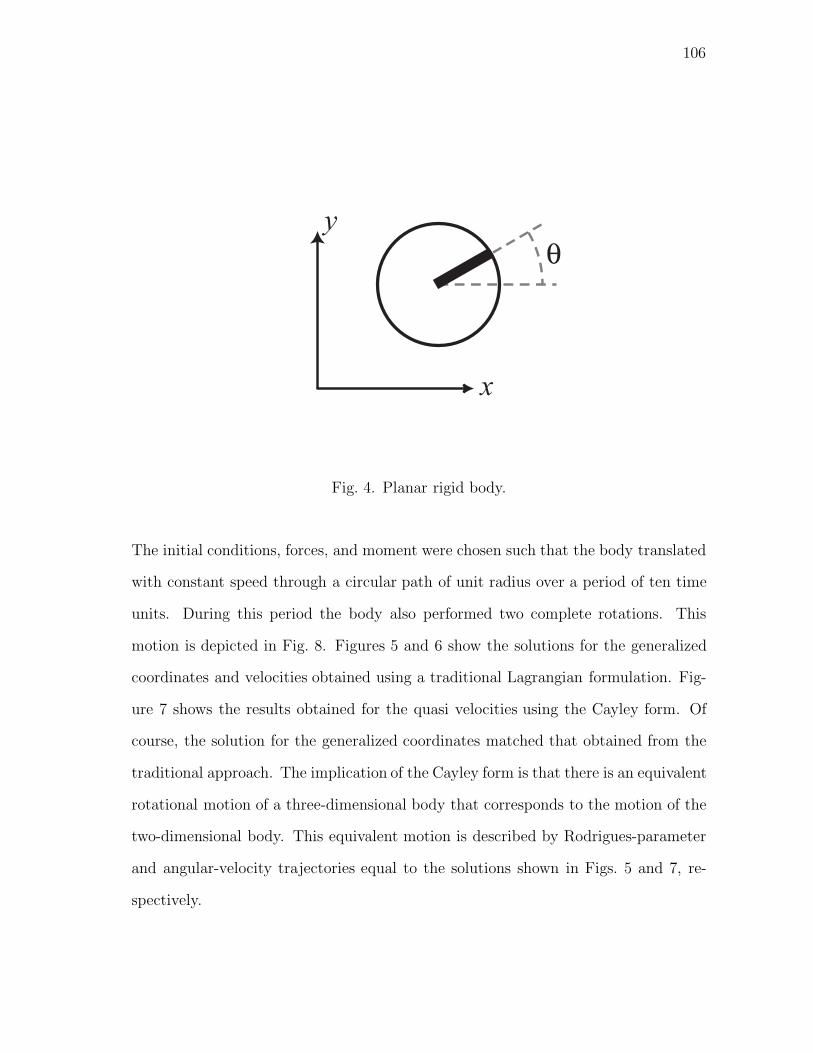
106

y

x

θ

Fig. 4. Planar rigid body.

The initial conditions, forces, and moment were chosen such that the body translated

with constant speed through a circular path of unit radius over a period of ten time

units. During this period the body also performed two complete rotations. This

motion is depicted in Fig. 8. Figures 5 and 6 show the solutions for the generalized

coordinates and velocities obtained using a traditional Lagrangian formulation. Fig-

ure 7 shows the results obtained for the quasi velocities using the Cayley form. Of

course, the solution for the generalized coordinates matched that obtained from the

traditional approach. The implication of the Cayley form is that there is an equivalent

rotational motion of a three-dimensional body that corresponds to the motion of the

two-dimensional body. This equivalent motion is described by Rodrigues-parameter

and angular-velocity trajectories equal to the solutions shown in Figs. 5 and 7, re-

spectively.

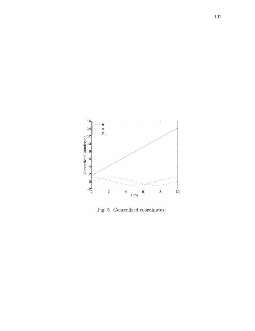
107

0 2 4 6 8 10−2

0

2

4

6

8

10

12

14

16

Gen

eral

ized

Coo

rdin

ates

Time

θxy

Fig. 5. Generalized coordinates.

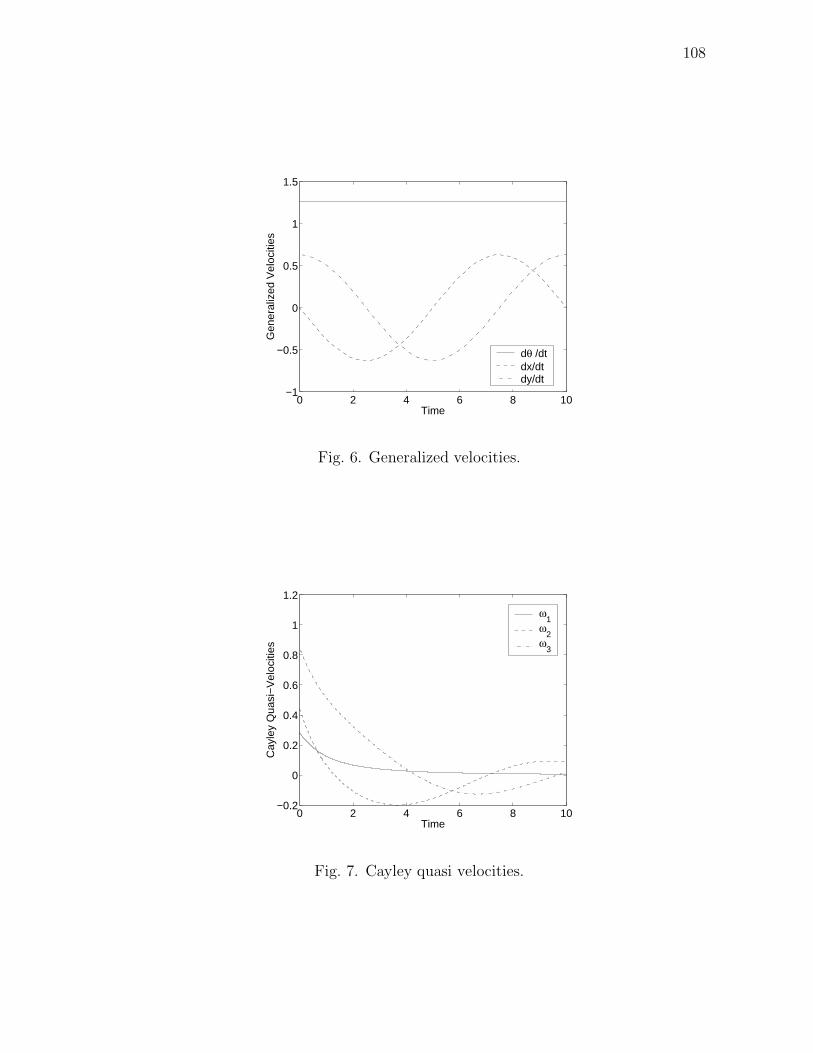
108

0 2 4 6 8 10−1

−0.5

0

0.5

1

1.5

Gen

eral

ized

Vel

ociti

es

Time

dθ /dtdx/dtdy/dt

Fig. 6. Generalized velocities.

0 2 4 6 8 10−0.2

0

0.2

0.4

0.6

0.8

1

1.2

Cay

ley

Qua

si−

Vel

ociti

es

Time

ω1

ω2

ω3

Fig. 7. Cayley quasi velocities.

109

x

y

t=10

t=0

t=2.5

t=5

t=7.5

Fig. 8. Example planar motion.

F. Discussion

This chapter has focused on the Cayley transform and the Cayley-transform kine-

matic relationship, and their use in developing the matrix form of the generalized

Euler equations of motion for N -dimensional rigid bodies. Related to these equa-

tions are the more general Euler-Poincare equations, which govern the motion of

left-invariant Lagrangian systems corresponding to general Lie groups [20, 36]. The

Hamel coefficients for an N -dimensional rigid body [15] were not explicitly encoun-

tered in the development because of the a priori decision to describe the system using

the Cayley orientation and kinematic variables.

The Cayley transform and the Cayley-transform kinematic relationship allowed

the realization that the motion of a general M-DOF (M = N(N − 1)/2) mechanical

system is related to the rotational motion of an N -dimensional rigid body. The

110

definition of an N -dimensional rigid body used here is kinematics based and hinges

on three facts: (1) the extended Rodrigues parameters, which completely describe

the configuration of the system, parameterize an N × N proper orthogonal matrix,

(2) an N ×N proper orthogonal matrix can be used to relate the orientation of one

N -dimensional reference frame to another, and (3) the orientation of a rigid body can

be defined as the orientation of a reference frame that is imbedded within it.

A useful relationship that was developed was the mapping of the skew-symmetric

matrix Q, which comprises the extended Rodrigues parameters for N -dimensional

spaces, to the matrix A that appears in the equation q = Aω. This mapping allows

the equations that govern the rotational motion of an N -dimensional rigid body to

be written in an M-dimensional vector form.

The benefits and implications of the relationship between M-DOF mechanical

systems and N -dimensional rigid bodies are still being investigated. Further research

is needed to investigate the extent to which the elegant tools that have been developed

for analyzing, controlling, and approximating the motion of three-dimensional rigid

bodies can be modified and applied to N -dimensional rigid bodies. The use of the

Cayley form will then allow these tools to be applied to a wide variety of physical

systems. Further research is also needed to investigate the ‘in-between’ M situation,

i.e., M = N(N−1)/2. One straightforward approach is to pad the vector of extended

Rodrigues parameters with additional fictitious coordinates until M = N(N − 1)/2.

The additional fictitious coordinates then represent constrained degrees of freedom.

111

CHAPTER VI

APPLICATION OF THE CAYLEY FORM TO GENERAL SPACECRAFT

MOTION

A. Introduction

Whereas the study of mechanics has been motivated by the desire to explain the three-

dimensional, physical universe, the mathematical models that have resulted are in no

way limited to three-dimensions. Higher-dimensional bodies can be kinematically

defined, and by assuming that principles such as conservation of angular momentum

and Hamilton’s principle apply in higher-dimensional spaces, their dynamics can also

be developed. In particular, one can consider the mechanics of an N -dimensional

rigid body, which can be defined as a system whose configuration can be completely

defined by an N ×N proper orthogonal matrix.

The descriptions of N -dimensional bodies are not simply mathematical curiosi-

ties: they can be used to describe real systems. This is done by linking the mo-

tion of general systems to the rotation of a higher-dimensional, rigid body. Three-

dimensional analogs to this approach have been used in the past. For example, Junk-

ins and Turner developed an analogy between spacecraft orbital motion and rigid

body rotations [42]. In that work a physical reference frame was defined using the

spacecraft position and velocity vectors. The orbital motion could then be studied

by describing the evolution of this frame. Because of the osculation constraint im-

plied in the definition of this frame, however, its motion does not fully capture the

orbital dynamics. The approach required explicit reintroduction of Newton’s second

law to describe the behavior of the radial distance. Additionally, whereas the kine-

112

matic analogy to a rigid body is clear, dynamically it was found that the gyroscopic

equations contained variable inertia due to changes in the radial distance.

This chapter presents a new analogy, called the Cayley form [16], between the

combined attitude and orbital motion of a spacecraft and rotational motion of a four-

dimensional, rigid body. In addition to incorporating both the attitude and orbital

motion, the new analogy more fully incorporates the dynamics in a general sense (i.e.,

osculation constraints are not imposed nor are explicit reintroductions required). In-

corporating both attitude and orbital motion in a single dynamic representation could

be seen as a disadvantage, because it does not take advantage of the decoupling that

occurs between these two motions for the special case of unforced dynamics. Many

other choices for representing translational and rotational motion, however, also ex-

hibit coupling in the motion variables, an example being the body components of

translational velocity [35]. The disadvantage is mitigated, however, by the fact that

for most spacecraft systems the attitude and orbital motions are in fact coupled by

forcing terms such as the rigid-body gravity potential or fixed-direction thrusters. A

second example is presented to further illustrate the new analogy. It involves the at-

titude motion of a satellite containing three momentum wheels, which is also related

to the rotational motion of a four-dimensional body. One potential advantage of the

Cayley form is that incorporating all system degrees of freedom into a single dynamic

representation can be beneficial in designing controllers. Although this is not fully

treated in this chapter, some preliminary results have demonstrated superior perfor-

mance in some cases for controllers designed using the Cayley form versus classical

approaches [43].

In each of these examples, the relations are made by associating each point in the

six-dimensional configuration space with a particular orientation in four-dimensional

space. Similar to the Junkins and Turner analogy, however, the new analogy does not

113

match all of the dynamics properties associated with rigid bodies. In the following

sections of the chapter the concepts of N -dimensional kinematics and dynamics are

reviewed, and their relationship to general systems is discussed. This is then used to

analyze general spacecraft motion.

B. Cayley Kinematics

The Cayley transform is a remarkable set of relationships between proper orthogonal

and skew-symmetric matrices [7]. Cayley discovered the forward relationship while

investigating some properties of “left systems” [8].

Forward: C = (I −Q) (I + Q)−1 = (I + Q)−1 (I − Q) (6.1)

Inverse: Q = (I −C) (I + C)−1 = (I + C)−1 (I − C) (6.2)

Here, C is an N × N proper orthogonal matrix, whereas Q is an N × N skew-

symmetric matrix, and I is the identity matrix. The matrix Q comprises a set of M

parameters that represent the orientation of an N -dimensional reference frame. In

fact q, the generating vector of Q, is the vector of extended Rodrigues parameters

(ERPs) for N -dimensional spaces [5, 6].

For N -dimensions the angular velocity is defined through the evolution of the

rotation matrix.

Ω = CT C (6.3)

In general, the angular velocity is a set of quasi velocities related to rotational mo-

tion (see Baruh, Section 7.6, pp. 378-380 [44]). Combining the angular velocity with

the Cayley transform produces the Cayley-transform kinematic relationships. These

relationships connect the derivatives of the M independent parameters of Q to the

114

angular-velocity matrix [12].

Ω = 2 (I + Q)−1 Q (I − Q)−1 (6.4)

Q =1

2(I + Q)Ω (I − Q) (6.5)

Equations (6.4) and (6.5) represent a linear mapping between the generalized veloci-

ties, Q, and a set of quasi velocities, Ω, for N -dimensional rotations. These equations

involve operations on N ×N matrices, but they can be rewritten in the more familiar

M-dimensional vector form.

qi = Aimωm (6.6)

This was carried out by Sinclair and Hurtado [16] using the numerical relative symbol

χ. The elements of A are given as a function of Q and the symbol χ in the following.

Aim =1

2

(δim − χi

vpχmvlQlp − 1

2χi

vpχmklQvkQlp

)(6.7)

C. N -Dimensional Rigid Body Dynamics

Based on the kinematics of N -dimensional bodies the question of studying the dy-

namics of N -dimensional bodies naturally arises. Indeed this was first suggested by

Cayley [8]. The equations of motion for rotations of N -dimensional bodies were first

found by Frahm [22], who approached the problem by considering the motion of a

collection of particles in N -dimensional space. More recently geometric methods have

been used to describe the free evolution of the angular-momentum matrix, L, of an

N -dimensional body [20,21,24,29]. That work has resulted in an elegant form for the

equations of motion called the Lax pair form.

The equations of motion for N -dimensional rigid bodies can also be achieved

using Lagrange’s equations in terms of quasi velocities. One method for doing this

uses Hamel coefficients [15]. The Hamel coefficients for N -dimensional rotations are

115

independent of the generalized coordinates and are given by the following.

γmvr =

1

2χm

ik (χvicχ

rck − χv

ckχric) (6.8)

These values are used in Lagrange’s equations to produce the vector form of the

equations of motion as shown in Table IV, where T is the kinetic energy as a function

of the generalized coordinates and angular velocity and gk is given below.

gk ≡ Ark

(fr +

∂T

∂qr

)(6.9)

Here, fr are the generalized forces and include potential and nonpotential forces.

An alternative choice would be to write the equations of motion in terms of the

Lagrangian and include only nonpotential terms in the generalized forces. Another

method for deriving the equations of motion arises from choosing the ERPs as gen-

eralized coordinates [16]. The Cayley kinematics can then be used directly to derive

the dynamic equations. Both methods produce the vector form of the equations of

motion shown in Table IV. Additionally, the tensor χ can be used to map the vector

form into the classic Lax pair matrix form using g as the generating vector for the

matrix G.

Whereas the kinematics and dynamics equations given in Table IV were origi-

nally derived to describe the motion of N -dimensional rigid bodies, they can also be

applied to any M-degree-of-freedom (DOF) mechanical system [16]. This leads to

the interesting result that the motion of any M-DOF mechanical system is equivalent

to the pure rotation of an N -dimensional rigid body. The simplest example of this

is the mapping from 1-DOF translation to 1-DOF rotation. Although these spaces

are topologically dissimilar, the equivalence is made possible by mapping the entire

translational space onto the singularity-free portion of the rotational space using a

parameterization with values including the entire real line. The M-dimensional vec-

116

tors of generalized coordinates and generalized velocities, q and q, for any system

can be used to generate skew-symmetric matrices Q and Q. The generalized coordi-

nates can then be substituted into the Cayley transform to generate an orthogonal

matrix, C, that describes the orientation of an equivalent N -dimensional rigid body.

The generalized coordinates of the system are equal to the ERPs of this rigid body.

Additionally, these generalized coordinates and velocities can be used to define a set

of Cayley quasi velocities via the Cayley-transform kinematic relationship. This set

of quasi velocities is equal to the angular velocity of the equivalent N -dimensional

rigid body. The Cayley quasi velocities are therefore governed by the N -dimensional

rotational equations of motion described above. This view of Lagrangian dynamics

is called the Cayley form [16].

D. General Spacecraft Motion

A large variety of mechanical systems can be studied using the Cayley form. This

section presents an example of the combined orbital and rotational motion of a space-

craft acted on by a gravity-gradient torque. For this problem a spherically-symmetric

Earth with gravitational parameter µ = 398600.4415 km3/s2 is assumed. Addition-

ally, higher-order effects such as higher-order gravitational torques and the influence

of attitude on the orbital motion are ignored. The satellite to be considered will have

a circular orbit with a radius of 8000 km.

The general motion of a three-dimensional rigid body has six degrees of freedom

and can therefore be related to the pure rotation of a four-dimensional rigid body. In

fact, the general motion of any N -dimensional body can be viewed as pure rotation

of an (N + 1)-dimensional body. The study of a three-dimensional rigid body using

the Cayley form is slightly complicated by the fact that three-dimensional rotational

117

motion is conventionally studied in terms of the three-dimensional angular velocity,

already a set of quasi velocities. Therefore, this portion of the problem must first

be converted back to a generalized-velocity expression. Throughout the example,

primes are used to denote three-dimensional rotational variables, as opposed to the

four-dimensional Cayley variables.

The generalized coordinates for the problem are [q]= [s′1 s′2 s′3 x1 x2 x3]T ,

where s′1, s′2, and s′3 are the three-dimensional modified Rodrigues parameters (MRPs)

and x1, x2, and x3 are the Cartesian position coordinates with respect to an Earth-

centered inertial reference frame, (e1, e2, e3), in units of Earth radii (ER=6378 km).

The choice of MRPs is somewhat arbitrary, and any three-parameter, attitude repre-

sentation could be used equally well. The MRPs relate the orientation of a body-fixed

frame(b1, b2, b3

)to the local vertical local horizontal (LVLH) frame. In this example

the LVLH frame is defined with a1 aligned with the radial direction, a3 oriented out

of the orbital plane, and a2 completing the orthogonal triad. The LVLH frame was

chosen as a reference to facilitate simulation over complete orbits while avoiding MRP

singularities.

In terms of the velocity, v (ER/sec), and the angular velocity of the body with

respect to the inertial reference, ω′ (rad/sec), the kinetic energy is given by the

following, where J ′ is the three-dimensional inertia tensor and m is the body’s mass.

T =1

2ω′TJ ′ω′ +

1

2mvT v (6.10)

118

Both ω′ and J ′ are coordinatized in the body frame. For the current example the

following inertia properties were used.

[J ′] =

⎡⎢⎢⎢⎢⎣100 0 0

0 200 0

0 0 200

⎤⎥⎥⎥⎥⎦ kgm2 (6.11)

For this choice of the inertia tensor the gravity-gradient stable configuration occurs

at alignment of the b1 and a1 vectors.

The angular velocity of the spacecraft with respect to the inertial reference is

the sum of the angular velocity with respect to the LVLH frame, ω′, and the angular

velocity of the LVLH frame with respect to the inertial frame, ω′. To simplify the

following developments the known solution for the angular velocity of the LVLH frame

in a circular orbit will be used directly.

ω′ = ω′ + ω′ = ω′ + nC1a3 (6.12)

Here C1 is the rotation matrix from the LVLH to the body frame and is a function of

the first three generalized coordinates, and n is the mean motion of the orbit. This

expression is used to expand the kinetic energy.

T =1

2ω′TJ ′ω′ + ω′TJ ′ω′ +

1

2ω′TJ ′ω′ +

1

2mvTv (6.13)

The three-dimensional angular velocity is related to the MRP rates by the famil-

iar kinematic differential equation.

s′ = A′ω′ ; ω′ = B′s′ (6.14)

119

[A′] =1

4

⎡⎢⎢⎢⎢⎣1 + s′1

2 − s′22 − s′3

2 2 (s′1s′2 − s′3) 2 (s′1s

′3 + s′2)

2 (s′1s′2 + s′3) 1 − s′1

2 + s′22 − s′3

2 2 (s′2s′3 − s′1)

2 (s′1s′3 − s′2) 2 (s′2s

′3 + s′1) 1 − s′1

2 − s′22 + s′3

2

⎤⎥⎥⎥⎥⎦ (6.15)

B′ = A′−1(6.16)

Using these three-dimensional kinematics, the kinetic energy can be defined in terms

of the generalized coordinates and velocities.

T0 (q, q) =1

2s′T B′TJ ′B′s′ + s′T B′TJ ′ω′ +

1

2ω′TJ ′ω′ +

1

2mvTv

=1

2qTJq + qTK +

1

2ω′TJ ′ω′ (6.17)

[J (q)] =

⎡⎢⎣ B′TJ ′B′ 0

0 mI

⎤⎥⎦ ; [K (q)] =

⎡⎢⎣ B′T J ′ω′

0

⎤⎥⎦ (6.18)

Here, the matrix I is the 3× 3 identity matrix. The linear mapping from the Cayley

quasi velocities to the generalized velocities, q = Aω, is found from the Cayley

kinematic definition and used to write the kinetic energy in terms of the generalized

coordinates and Cayley quasi velocities.

T1 (q,ω) =1

2ωTAT JAω + ωTAT K +

1

2ω′TJ ′ω′

=1

2ωiAliJlmAmjωj + ωiAliKl +

1

2ω′

iJ′ijω

′j (6.19)

The necessary partial derivatives of T1 can now be taken. Note that J and K

are functions of the first three generalized coordinates and are not constant.

∂T1

∂qr=

1

2ωi

(∂Ali

∂qrJlmAmj + Ali

∂Jlm

∂qrAmj + AliJlm

∂Amj

∂qr

)ωj

+ ωi

(∂Ali

∂qrKl + Ali

∂Kl

∂qr

)+∂ω′

i

∂qrJ ′

ij ω′j (6.20)

∂T1

∂ωr= AlrJlmAmjωj + AlrKl (6.21)

120

d

dt

(∂T1

∂ωk

)=AlkJlmAmjωj + AlkJlmAmjωj + AlkJlmAmjωj

+ AlkJlmAmjωj + AlrKl + AlrKl (6.22)

The derivatives of A are computed using the chain rule.

Alk =∂Alk

∂qsqs =

∂Alk

∂qsAstωt (6.23)

The partial derivatives of A are directly evaluated from Eq. (6.7). The derivatives of

J must now be considered.

∂Jlm

∂qr=

⎡⎢⎣ ∂B′∂qr

TJ ′B′ + B′T J ′ ∂B′

∂qr0

0 0

⎤⎥⎦lm

(6.24)

Jlm =∂Jlm

∂qiqi (6.25)

The derivatives of B are computed in the following manner.

∂B′

∂qr= −B′∂A′

∂qrB′ (6.26)

The derivatives of K are also computed.

∂Kl

∂qr=

⎡⎢⎣ ∂B′T∂qr

J ′ω′ + B′T J ′ ∂ω′∂qr

0

⎤⎥⎦l

(6.27)

Kl =∂Kl

∂qiqi (6.28)

Finally, the partial derivatives of A′ are directly evaluated from Eq. (6.15), and clearly

only the derivatives with respect to the first three generalized coordinates are nonzero.

Similarly, the partial derivatives of ω are evaluated by directly taking the derivatives

of the rotation matrix C1 with respect to the MRP coordinates.

121

The generalized forces in terms of the generalized velocities are related to the

moment vector M (coordinatized in the body frame) and the force vector F (co-

ordinatized in the inertial frame) applied to the body. These are computed using

the familiar gravitational models where the vector r has components consisting of

the three position coordinates and a magnitude of r, and C2 is the rotation matrix

from the inertial to LVLH frame. This matrix is assembled from the inertial compo-

nents of r and v. Additionally, a damping moment is included with the coefficient

k = 0.1 kg m2/s to simulate a nutation damper onboard the spacecraft.

M = 3µ

r3a × J ′a − kω′ ; a = C1C2r/r (6.29)

F = −µmr3

r (6.30)

The generalized forces with respect to the first and fourth generalized coordinates are

shown below.

f1 = F T ∂v

∂q′1+ MT ∂ω′

∂q′1= MTB′b1 (6.31)

f4 = F T ∂v

∂x1+ MT ∂ω′

∂x1= F T e1 (6.32)

The other generalized forces are similar to these two.

[f ] =[MTB′ F T

]T(6.33)

Using Eqs. (6.20) to (6.33), the equations of motion as shown in Table IV can be

assembled and solved for the components ωj . These equations can then be integrated

to solve directly for the motion of the satellite in terms of the generalized coordinates

and the Cayley quasi velocities. Due to the coupling of all six degrees of freedom,

however, these equations are somewhat more difficult to integrate than the traditional

implementation. Solving for ω requires taking the inverse of a 6 × 6 matrix. The

difficulty can be somewhat relieved through scaling. Integrating over one orbital

122

period using the Matlab algorithm ODE45 required 769 integration steps for the

traditional Euler and orbit equations and 989 integration steps for the Cayley form,

with identical settings. Integration of the traditional implementation can also be

used to verify the results from the Cayley form. The Cayley-transform kinematic

relationship can be applied to the results of the traditional equations of motion to

compute the quasi velocities from the generalized coordinates and velocities. The

results of these numerical solutions are shown in Figs. 9 and 10.

Figure 9 shows the solutions for the generalized coordinates, three-dimensional

angular velocity, and translational velocity. The simulation results represent the

motion of the satellite through one complete orbit around the Earth. The orbit has

an inclination of thirty degrees. The spacecraft is initially rotated 10 degrees relative

to the LVLH frame. Due to the initial conditions and the gravity-gradient torque the

spacecraft remains within 33 degrees of the LVLH reference. As can be seen by s′3 in

Fig. 9, for the first sixty minutes the spacecraft attitude lags behind the LVLH frame

due to the damping moment. As this happens the gravity-gradient moment increases

and during the second sixty minutes the spacecraft begins to restore alignment with

the LVLH frame. Figure 10 shows the results obtained for the Cayley quasi velocities.

The implication of the Cayley form is that there is an equivalent rotational motion of

a four-dimensional body that corresponds to the general motion of the satellite. For

this equivalent motion the six components of the ERPs have trajectories equal to the

solutions shown in Fig. 9 for the MRPs and position coordinates. The angular-velocity

components are equal to the trajectories shown in Fig. 10.

These results also demonstrate some interesting features of the Cayley form. One

feature is due to the nondimensionality of the ERPs. Because the Cayley form sets the

generalized coordinates of the system numerically equal to the ERPs of the equivalent

N -dimensional rotation, the mapping is sensitive to the choice of coordinates and

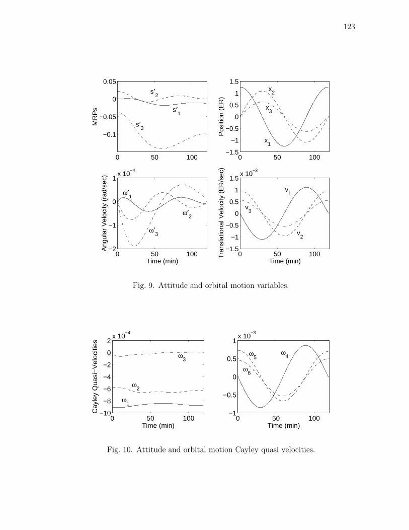
123

0 50 100

−0.1

−0.05

0

0.05

MR

Ps s′

1

s′2

s′3

0 50 100−1.5

−1

−0.5

0

0.5

1

1.5

Pos

ition

(E

R)

x1

x2

x3

0 50 100−2

−1

0

1x 10

−4

Ang

ular

Vel

ocity

(ra

d/se

c)

Time (min)

ω′1

ω′2

ω′3

0 50 100−1.5

−1

−0.5

0

0.5

1

1.5x 10

−3

Tra

nsla

tiona

l Vel

ocity

(E

R/s

ec)

Time (min)

v1

v2

v3

Fig. 9. Attitude and orbital motion variables.

0 50 100−10

−8

−6

−4

−2

0

2x 10

−4

Cay

ley

Qua

si−

Vel

ociti

es

Time (min)

ω1

ω2

ω3

0 50 100−1

−0.5

0

0.5

1x 10

−3

Time (min)

ω4ω

5

ω6

Fig. 10. Attitude and orbital motion Cayley quasi velocities.

124

units used to describe the original system. For example, the use of kilometer units

to describe the above orbital dynamics would produce a different time history of the

ERPs and thus a different four-dimensional rotation.

Another feature has to do with the presence of singularities in the ERP de-

scription of N -dimensional orientation. Exactly analogous to the familiar Rodrigues

parameter singularities, certain N ×N proper orthogonal matrices result in ERP el-

ements that tend toward infinity [2]. Because in the Cayley form the ERPs are equal

to the generalized coordinates of the original system, though, these rotation variables

can only go to infinity if the original generalized coordinates do the same. The MRPs

used in the above example suffer from singularities in the conventional equations of

motion; however, applying the Cayley form does not add any new singularities. For

cases in which the generalized coordinates of the original problem are guaranteed to

avoid divergence to infinity, then the Cayley form will automatically be constrained

to avoid the singular N -dimensional configurations.

E. Satellite with Three Momentum Wheels

The Cayley form can also be applied to multibody systems. Again, the dimension of

the equivalent body in pure rotation is a function of the total number of degrees in

freedom of the system. Here, the rotational motion of a satellite with three momentum

wheels will be considered. Similar to the previous example, this system has six degrees

of freedom and is equivalent to the rotational motion of a four-dimensional body.

The generalized coordinates for this problem consist of two sets: (1) the Ro-

drigues parameters describing the orientation of an axes set(b1, b2, b3

)attached to

the satellite body relative to an inertial set (e1, e2, e3) and (2) the angles describing

125

the orientation of each wheel relative to the satellite.

[q] = [q′1 q′2 q′3 θ1 θ2 θ3]T ≡ [q′T θT

]T(6.34)

The body axes attached to the satellite are assumed to be the principal axes of the

satellite body. The three wheels are identical, symmetric, and aligned with the body

axes. Additionally, for convenience, the wheels are assumed to be located at the

system center of mass.

The kinetic energy of the system is given by the following.

T =1

2ωT

b Jbωb +1

2ωT

w1Jw1ωw1 +1

2ωT

w2Jw2ωw2 +1

2ωT

w3Jw3ωw3 (6.35)

The subscript b refers to the satellite body and the subscripts w1, w2, and w3 refer to

the three wheels. The angular velocity of wheel 1, for example, is ωw1 = ωb+θ1b1. For

simplicity the inertia of the satellite body was chosen as Jb = 100I kgm2. The axial

component of inertia for each wheel was chosen to be Ja = 10kg m2, and the transverse

component was Jt = 1kg m2. For convenience, the sum J ′ = Jb + Jw1 + Jw2 + Jw3

is defined. The kinetic energy in terms of the body angular velocity and the wheel

angle rates is shown below.

T =1

2ωT

b J ′ωb + JaωTb θ +

1

2Jaθ

T θ (6.36)

Using the three-dimensional kinematics this is converted to an expression in terms of

the generalized coordinates and velocities.

T0 =1

2

[q′T θT

]⎡⎢⎣ B′T J ′B′ JaB′T

JaB′ JaI

⎤⎥⎦⎡⎢⎣ q′

θ

⎤⎥⎦ ≡ 1

2qT Jq (6.37)

126

Again, this expression is rewritten in terms of the Cayley quasi velocities using the

four-dimensional Cayley kinematics.

T1 (q,ω) =1

2ωTAT JAω =

1

2ωiAliJlmAmjωj (6.38)

The derivatives of T1 are computed in an identical manner as was done in the previous

example. These expressions are somewhat simpler than in the previous example due

to the natural form of the kinetic energy in this problem. Another difference is that

the derivatives of J now have the following form.

∂Jlm

∂qr=

⎡⎢⎣ ∂B′∂qr

TJ ′B′ + B′TJ ′ ∂B′

∂qrJa

∂B′T∂qr

Ja∂B′∂qr

0

⎤⎥⎦lm

(6.39)

The generalized forces are computed considering an external moment M (co-

ordinatized in the body frame) and internal moments u1 = u1b1, u2 = u2b2, and

u3 = u3b3. The internal moments are applied to each wheel, respectively. The exter-

nal moment and internal moments (−u = −u1 − u2 − u3) are applied to the satellite

body. The generalized forces associated with the first and fourth generalized velocities

are shown below.

f1 = (M − u)T ∂ωb

∂q′1+ uT

1

∂ωw1

∂q′1+ uT

2

∂ωw2

∂q′1+ uT

3

∂ωw3

∂q′1= MT ∂ωb

∂q′1= MTB′b1

(6.40)

f4 = (M − u)T ∂ωb

∂θ1

+ uT1

∂ωw1

∂θ1

+ uT2

∂ωw2

∂θ1

+ uT3

∂ωw3

∂θ1

= u1 (6.41)

The other generalized forces are similar to these two: [f ] =[MTB′ uT

]T.

Using the derivatives of T1 and the generalized forces, the equations of motion

can be assembled and solved for the components ωj . Figures 11 and 12 show sim-

ulation results from the integration of these equations of motion and the Cayley

127

kinematic equations. The initial conditions were chosen such that the body was ini-

tially rotating about the b1 axis. Beginning at time zero, a constant moment of 5

Nm is applied to the second momentum wheel. The external moment was set to

zero in the simulation. Figure 11 shows the solutions for the generalized coordinates,

three-dimensional angular velocity, and wheel-angle rates obtained using a traditional

formulation. Figure 12 shows the results obtained for the quasi velocities using the

Cayley form. Again, the implication of the Cayley form is that there is an equivalent

rotational motion of a four-dimensional body that corresponds to the motion of the

satellite and momentum-wheel system. For this equivalent motion the six compo-

nents of the ERPs have trajectories equal to the solutions shown in Fig. 11 for the

Rodrigues parameters and wheel angles. The angular velocity components are equal

to the trajectories shown in Fig. 12.

F. Discussion

The most common representation of motion that is applied to general systems is the

motion of a point in M-dimensional state space. The application of the Cayley form

in this chapter, however, is one example of the broad set of other possible represen-

tations. Another, more famous, example is the use of the Frenet formulas to describe

particle motion in terms of a rotating reference frame, and in fact the approach of

Junkins and Turner [42] is an example of this. The classic Frenet frame is defined by

the velocity and acceleration vectors, whereas Junkins and Turner used position and

velocity. Their analogy and the Cayley form can both be used to represent three-

dimensional translations as three-dimensional rotations. Therefore, combined orbital

and attitude motion, the rotation of two rigid bodies, and the rotation of a four-

dimensional rigid body represent three members of a family of systems that are in a

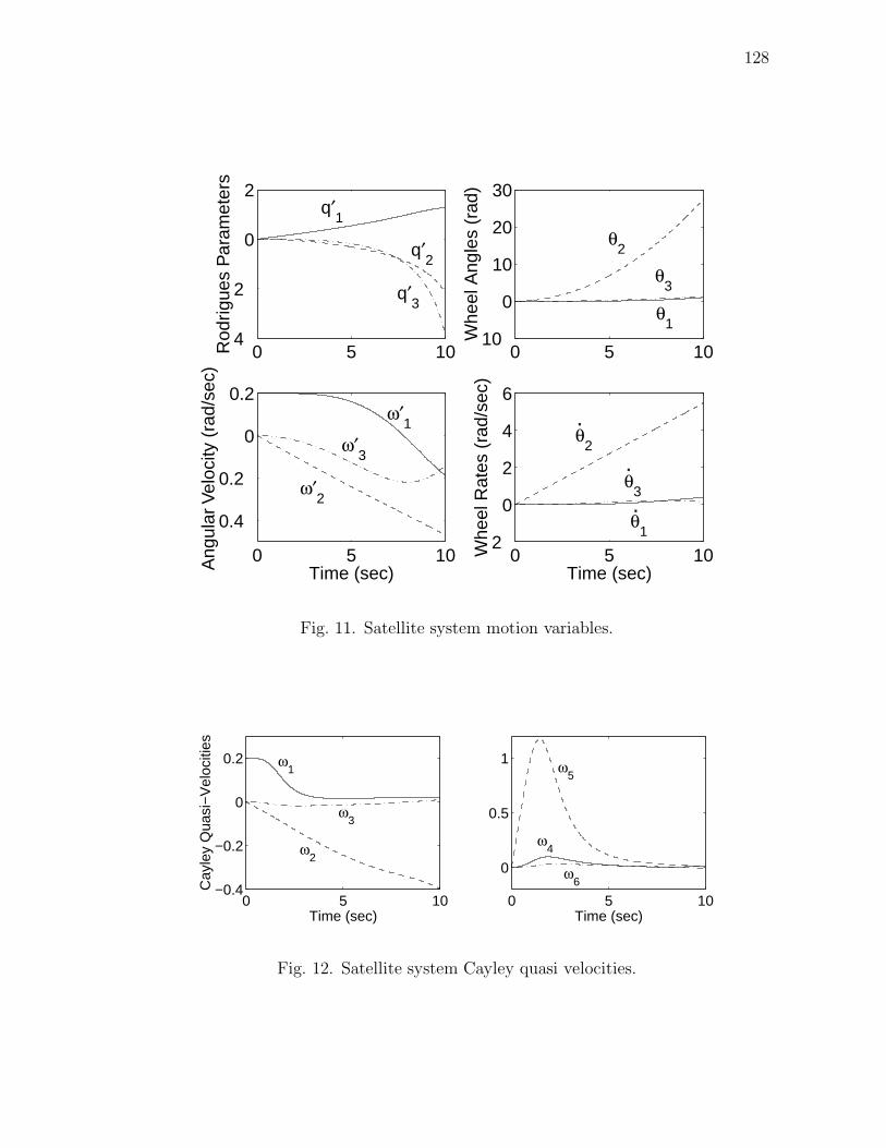
128

0 5 104

2

0

2

Rod

rigue

s P

aram

eter

sq′

1

q′2

q′3

0 5 1010

0

10

20

30

Whe

el A

ngle

s (r

ad)

θ1

θ2

θ3

0 5 10

0.4

0.2

0

0.2

Ang

ular

Vel

ocity

(ra

d/se

c)

Time (sec)

ω′1

ω′2

ω′3

0 5 102

0

2

4

6

Whe

el R

ates

(ra

d/se

c)

Time (sec)

θ1

θ2

θ3

.

.

.

Fig. 11. Satellite system motion variables.

0 5 10−0.4

−0.2

0

0.2

Cay

ley

Qua

si−

Vel

ociti

es

Time (sec)

ω1

ω2

ω3

0 5 10

0

0.5

1

Time (sec)

ω4

ω5

ω6

Fig. 12. Satellite system Cayley quasi velocities.

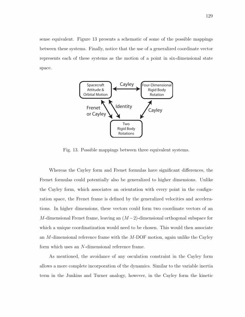
129

sense equivalent. Figure 13 presents a schematic of some of the possible mappings

between these systems. Finally, notice that the use of a generalized coordinate vector

represents each of these systems as the motion of a point in six-dimensional state

space.

SpacecraftAttitude &

Orbital Motion

Four-DimensionalRigid Body

Rotation

TwoRigid BodyRotations

Identity

Cayley

CayleyFrenetor Cayley

Fig. 13. Possible mappings between three equivalent systems.

Whereas the Cayley form and Frenet formulas have significant differences, the

Frenet formulas could potentially also be generalized to higher dimensions. Unlike

the Cayley form, which associates an orientation with every point in the configu-

ration space, the Frenet frame is defined by the generalized velocities and accelera-

tions. In higher dimensions, these vectors could form two coordinate vectors of an

M-dimensional Frenet frame, leaving an (M−2)-dimensional orthogonal subspace for

which a unique coordinatization would need to be chosen. This would then associate

an M-dimensional reference frame with the M-DOF motion, again unlike the Cayley

form which uses an N -dimensional reference frame.

As mentioned, the avoidance of any osculation constraint in the Cayley form

allows a more complete incorporation of the dynamics. Similar to the variable inertia

term in the Junkins and Turner analogy, however, in the Cayley form the kinetic

130

energy was found to be a function of the generalized coordinates. While both analogies

match the kinematic properties of rigid bodies, the dynamic properties of rigid bodies

(i.e., constant inertia) do not precisely hold. The analogies can only go so far.

G. Conclusions

In this chapter the kinematics and dynamics of N -dimensional bodies have been

discussed and their application to general spacecraft motion has been demonstrated.

This Cayley form results in new equations of motion for the orbital and attitude

dynamics. A perceived disadvantage of this form is the resulting coupling that takes

place between the attitude and orbital motion. This coupling, however, reveals a

possible application of the Cayley form. Many special techniques have been developed

for attitude determination and control in three-dimensional space. If these techniques

can be generalized to higher dimensions, then the Cayley form can be used to apply

them to a broader class of mechanical systems. Although not treated in this chapter,

some preliminary results involving feedback control using the Cayley form have been

developed.

Possible applications include combined attitude and orbit determination and

control. This could be of particular interest for systems that already exhibit a high

degree of attitude and orbital coupling, such as low-thrust, fixed thrust-direction

spacecraft and very large spacecraft subject to higher-order gravitational torques and

forces. A more theoretical direction for future research is the study of the relation

of ERPs to the principal planes and angles of N -dimensional orientation and the

interpretation of ERP singularities.

131

CHAPTER VII

STABILIZATION AND CONTROL OF DYNAMICAL SYSTEMS IN THE

CAYLEY FORM

A. Introduction

Beginning with Euler the rotational motion of three-dimensional bodies has been

studied for over two hundred years. The development of spacecraft technology over

the past fifty years has inspired a continuing focus on this problem that has produced

many significant developments in attitude representations and control. An example

of this, that will be a focus of this chapter, is the proof discovered by Tsiotras for

global asymptotic stability using linear feedback of angular velocity and the Rodrigues

parameters [45, 46].

Although not receiving as much attention, the study of N -dimensional rotational

motion also has an impressive history [1, 8, 22, 23]. Developments have been made to

generalize many of the kinematic and dynamical concepts from three-dimensional

rotations to higher dimensions [2,5,6,15,21,24,28]. Another interesting aspect of this

topic is that the resulting equations of motion can be used to describe the behavior of

real physical systems. One example of this is called the Cayley form and represents

the generalized coordinates and quasi velocities of a general system as the extended

Rodrigues parameters (ERPs) and angular velocity of an N -dimensional rotating

body [16, 17].

The wealth of work that has been done for three-dimensional attitude control

and the ability to represent general systems as N -dimensional rigid bodies motivates

the idea of generalizing some of these three-dimensional results to higher dimensions.

This chapter presents some investigations for extending Lyapunov and optimal control

132

results to N -dimensional rotations. Further investigations are also conducted into the

application of these results to natural dynamical systems.

Section B of this chapter reviews the set of quasi velocities used in the Cayley

form related to N -dimensional rotations. Section C reviews some elegant attitude

control results discovered by Tsiotras, approaching them as a three-dimensional spe-

cial case of the Cayley form. Next, the equations of motion for N -dimensional rota-

tions are covered and the corresponding work/energy-rate expression is developed in

Section D. Then, it is shown in Section E how properties of the N -dimensional kine-

matics disallow an exact generalization of Tsiotras’s results, and several alternative

controller designs are presented. An alternative set of quasi velocities is presented in

Section F that does provide globally asymptotically stable linear feedback. In Sec-

tions G and H the controllers from the Cayley form are analyzed for their optimality

and performance.

B. Definition of Cayley Quasi Velocities

The Cayley form describes N -dimensional rotations using the ERPs, Q or q, which

are related to the N -dimensional orientation matrix by the Cayley transform. The

Cayley-transform kinematic relationship gives a mapping for N -dimensional rotations

from the ERP rates to the angular velocity in skew-symmetric form [12].

Ω = 2 (I + Q)−1 Q (I −Q)−1 ≡ 2B+QB− (7.1)

Q =1

2(I + Q)Ω (I − Q) ≡ 1

2A+ΩA− (7.2)

In the Cayley-form representation of mechanical systems these expressions also form

the definition of the Cayley quasi velocities, Ω. For an M-degree-of-freedom (DOF)

system, the Cayley form equates the generalized coordinates of the system with the

133

ERPs of an N -dimensional rotation, and the Cayley quasi velocities are equivalent to

the N -dimensional angular velocity. From these relationships the linear mapping be-

tween the vector forms of the ERP rates and the angular velocity can be found, which

also serves as the traditional vector-transformation definition of the quasi velocities.

ω = Bq ; q = Aω (7.3)

Relating Eq. (7.2) and the second of Eqs. (7.3) the elements of A are found.

Qvp =1

2A+

vkΩklA−lp (7.4)

χjvpqj =

1

2A+

vkχmklωmA

−lp (7.5)

2δij qj =1

2χi

vpχmklA

+vkA

−lpωm (7.6)

qi =1

4χi

vpχmklA

+vkA

−lpωm (7.7)

Aim ≡ 1

4χi

vpχmklA

+vkA

−lp =

1

4χi

vpχmkl (δvk +Qvk) (δlp −Qlp)

=1

4χi

vpχmkl (δvkδlp − δvkQlp + δlpQvk −QvkQlp) (7.8)

The first term of Eq. (7.8) simplifies as follows.

1

4χi

vpχmklδvkδlp =

1

4χi

vpχmvp =

1

2δim (7.9)

The second term of Eq. (7.8) can also be simplified.

−1

4χi

vpχmklδvkQlp = −1

4χi

vpχmvlQlp (7.10)

The third term is identical to the second.

1

4χi

vpχmklδlpQvk =

1

4χi

vpχmkpQvk =

1

4χi

pvχmlvQpl = −1

4χi

vpχmvlQlp (7.11)

134

Substituting these terms back into Eq. (7.8) gives the following expression for the

elements of A.

Aim =1

2

(δim − χi

vpχmvlQlp − 1

2χi

vpχmklQvkQlp

)(7.12)

For the special case N = 3, the equation for the elements of A can be simplified

by substituting εijk for χjik.

Aim =1

2

(δim − εvipεvmlQlp − 1

2εvipεkmlQvkQlp

)(7.13)

The “ε-δ identity” can be applied to the second term of this equation. The fact that

Qii equals zero, because Q is skew-symmetric, is also used.

εvipεvmlQlp = (δimδpl − δilδpm)Qlp = −Qim (7.14)

The third term of Eq. (7.13) can also be rewritten using the generalized Kronecker

delta [32].

εvipεkml = δkmlvip =

∣∣∣∣∣∣∣∣∣∣δvk δik δpk

δvm δim δpm

δvl δil δpl

∣∣∣∣∣∣∣∣∣∣= δvkδimδpl − δvkδpmδil + δikδpmδvl − δikδvmδpl + δpkδvmδil − δpkδimδvl (7.15)

The third term of Eq. (7.13) therefore becomes the following.

εvipεkmlQvkQlp = QviQvm +QmpQip − δimQvpQvp = 2QviQvm − δimQvpQvp (7.16)

135

This expression is now rewritten in terms of the vector elements qj and the ε-δ identity

is used once again.

εvipεkmlQvkQlp = 2εvriqrεvsmqs − δimεvrpqrεvspqs

= 2 (δrsδim − δrmδis) qrqs − δim (δrsδpp − δrpδsp) qrqs

= 2δimqrqr − 2qiqm − 3δimqrqr + δimqpqp

= −2qiqm (7.17)

Equations (7.14) and (7.17) are now substituted into Eq. (7.13) to give the familiar

form for the mapping from the angular velocity to the Rodrigues parameter rates [38].

Aim =1


C. Linear Rodrigues-Parameter Feedback

In the previous section a simple form was found for the elements, Aim, of the matrix

that maps the angular velocity to the Rodrigues parameter rates for N = 3. In this

section several special properties of this three-dimensional form will be demonstrated

that lead to a proof of global asymptotic stability for linear feedback of the Rodrigues

parameters and angular velocity. First, for this special case it will be shown that q

is an eigenvector of AT , using the fact that the product Qq equals zero.

[ATq

]m

= Aimqi =1

2(qm +Qimqi + qiqmqi) =

1

2(1 + qiqi) qm ≡ λqm (7.19)

Therefore, the eigenvalue associated with q is 12(1 + qiqi).

A similar derivation can be used to show that q is also an eigenvector of A. This

fact, however, can also be understood from a physical interpretation. Consider the

situation of ω being aligned with q, ω = αq. In this case the body is simply “spinning

up” because the vector of Rodrigues parameters is always parallel with the principal

136

axis of rotation. Therefore, the direction of q is constant, and only its magnitude is

changing. This means that q is also parallel to q, q = αλq. In this case, the second

of Eqs. (7.3) becomes the following.

αλq = A (αq) (7.20)

The proportionality factors α and λ are simply scalars, and thus q being an eigen-

vector of A is physically expected.

The eigenvalue of AT associated with q has the following remarkable property.

d

dt

(1

2(1 + qiqi)

)= qiqi = qiAimωm =

1

2(1 + qiqi) qmωm (7.21)

Equations (7.19) and (7.21) allow the following elegant proof discovered by Tsiotras

[45]. Consider the following Lyapunov function where the first term is the rotational

kinetic energy of a three-dimensional rigid body and the second is a fictitious potential

energy.

V =1

2ωiJijωj + ln (1 + qiqi) (7.22)

Here, Jij are the elements of the principal inertia matrix. As it will be seen, the

kinetic-energy term of the Lyapunov functions leads to a stabilization term of the

control law that brings the body to rest, and the potential-energy term leads to

a regulation control term that drives the body to the reference orientation. Using

Euler’s equations the time derivative of the kinetic energy is given by the following.

d

dt

(1

2ωiJijωj

)= ωiJijωj = ωj

(εjilJikωlωk + f

(ω)j

)= ωjf

(ω)j (7.23)

Here, f(ω)j are the applied moment components acting on the body and are assumed

to be control torques. This leads to the following result for the Lyapunov function

137

derivative.

V = ωif(ω)i +

ddt

(1 + qiqi)

1 + qiqi= ωif

(ω)i + qiωi (7.24)

If the control elements, f(ω)i , are chosen to make Eq. (7.24) negative semi-definite,

then the system will be globally asymptotically stable by LaSalle’s theorem. This can

be done in the following fashion.

V = ωif(ω)i + qiωi ≡ −ωiωi (7.25)

f(ω)i = −ωi − qi (7.26)

Therefore, Eq. (7.26) is a linear, globally asymptotically stable controller for the

attitude stabilization and regulation of three-dimensional bodies. This controller is

very attractive, and the following sections will attempt to determine if it can be

extended to guarantee global asymptotic stability for general N -dimensional bodies

or M-DOF systems.

D. Work/Energy-Rate Expression for N -Dimensional Dynamics

An important step in the developments of the previous section is the simplification

of the derivative of the kinetic energy under Euler’s equation. To generalize these

results it needs to be determined if these terms follow similar simplifications under

the general N -dimensional dynamics. In this section the work/energy-rate expression

will be developed for the general N -dimensional dynamics, recalling that by using

the Cayley form these dynamics can represent any M-DOF physical system. These

equations of motion can be derived using Lagrange’s equations for quasi velocities,

which are also known as Poincare’s equations [35].

d

dt

(∂T

∂ωk

)+ γr

kaωa∂T

∂ωr− Ark

∂T

∂qr= f

(ω)k (7.27)

138

Here, T = T (q,ω) is the kinetic energy, and the components f(ω)k can either be

considered as the moments applied to an N -dimensional rigid body or functions of

the generalized forces, f , applied to an M-DOF physical system: f(ω)k = Ajkfj.

Therefore, these components f(ω)k are the generalized forces associated with the quasi

velocities, and are here simply called the quasi forces. The three-index symbol γrka

that appears in Eq. (7.27) represents the Hamel coefficients which are given by the

following expression [15].

γmvr =

1

2χm

ik (χvicχ

rck − χv

ckχric) (7.28)

The kinetic energy of a natural system is represented using the Cayley form as

follows.

T =1

2ωiJij(q)ωj (7.29)

Here, Jij are the elements of the symmetric mass matrix associated with the Cayley

quasi velocities. For an N -dimensional rotating body, J can be selected without loss

of generality to be diagonal and is independent of the generalized coordinates. For

other systems mapped by the Cayley form, however, these properties do not need to

be assumed. Additionally because the current interest is in feedback controllers, it

is assumed that the system is not explicitly time dependent, and thus the focus is

placed on natural systems.

To evaluate Lagrange’s equations the following derivatives of T are taken.

∂T

∂qr=

1

2ωi∂Jij

∂qrωj (7.30)

∂T

∂ωr= Jrjωj (7.31)

d

dt

(∂T

∂ωk

)= Jkj ωj +

∂Jkj

∂qsqsωj (7.32)

139

These are substituted into the equations of motion.

Jkj ωj +∂Jkj

∂qs

qsωj + γrkaωaJrjωj − 1

2Arkωi

∂Jij

∂qr

ωj = f(ω)k (7.33)

Similar to the previous section the time derivative of the kinetic energy needs to

be found due to these dynamic equations.

T =∂T

∂ωrωr +

∂T

∂qrqr = Jrjωjωr +

1

2ωi∂Jij

∂qrωj qr

=

(−∂Jjk

∂qsqsωk − γr

jaωaJrkωk +1

2Arjωi

∂Jik

∂qrωk + f

(ω)j

)ωj +

1

2ωi∂Jij

∂qrωj qr

= −∂Jjk

∂qsqsωkωj − γr

jaωaJrkωkωj +1

2ωi∂Jik

∂qrωkqr + f

(ω)j ωj +

1

2ωi∂Jij

∂qrωj qr

= −γrjaωaJrkωkωj + f

(ω)j ωj (7.34)

This expression is further simplified by considering the definition of the Hamel coef-

ficients in Eq. (7.28) and the properties of χ.

γrjaωaJrkωkωj =

1

2Jrkχ

rde

(χj

dcχace − χj

ceχadc

)ωaωkωj

=1

2Jrkχ

rde

(χj

dcχaceωaωj − χj

ceχadcωaωj

)ωk

= −1

2Jrkχ

red

(χj

dcχaceωaωj − χj

ceχadcωaωj

)ωk

= −1

2Jrkχ

rde

(χj

ecχacdωaωj − χj

cdχaecωaωj

)ωk

= −1

2Jrkχ

rde

(χj

ceχadcωaωj − χj

dcχaceωaωj

)ωk

= −1

2Jrkχ

rde

(χa

ceχjdcωjωa − χa

dcχjceωjωa

)ωk = 0 (7.35)

Hence the Hamel coefficient term is nonworking. This leaves the identical work/

energy-rate expression as the three-dimensional special case: T = ωjf(ω)j . For the

three-dimensional case several feedback attitude controllers have been developed using

a Lyapunov function consisting of the sum of the kinetic energy and various fictitious

140

potential energies. The next section will demonstrate the behavior of some of these

potential energies under the general N -dimensional Cayley kinematics.

E. Feedback Control for N -Dimensional Rotations

Recall from an earlier section that a key to developing the linear controller for N = 3

was the recognition that q is an eigenvector of AT . Also, for the three-dimensional

special case it was noted that q is an eigenvector of both AT and A. To extend these

developments to higher dimensions it will be determined if these properties are true

in general. This can be approached in general using the definition of A.

[AT q

]m

= Aimqi =1

2

(δimqi − χi

vpχmvlQlpqi − 1

2χi

vpχmklQvkQlpqi

)(7.36)

Using the properties of the Kronecker delta and χ it can be seen that Aimqi = Amiqi.

This is obviously true for the first term above, and similar to the three-dimensional

case, the second term is equal to zero as shown below. The third term is demonstrated

through manipulation of the repeated indices as also shown below.

−χivpχ

mvlQlpqi = χm

vlQplQvp = −χmlvQlpQpv = −χm

vlQvpQpl = 0 (7.37)

−1

2χi

vpχmklQvkQlpqi = −1

2χi

klχmvpQkvQplqi = −1

2χi

klχmvpQvkQlpqi (7.38)

Therefore, q is an eigenvector of AT if and only if it is also an eigenvector of A. For

q to be an eigenvector of A the following relation must be true: Amiqi = λqm. From

Eq. (7.36) it is seen that the term linear in qi obviously satisfies this relation, and the

quadratic term has been shown to equal zero. Clearly the cubic term is critical.

Similar to the physical description of N = 3, this eigenproblem can be studied

by considering the special case for which the angular velocity is proportional to the

ERPs: ω = αq. Assuming q is indeed an eigenvector of A, then in this case the

141

derivatives of these parameters will also be proportional to the angular velocity.

q = Aω = αAq = αλq = λω (7.39)

Here, λ is the eigenvalue of A assumed to be associated with q. This proportionality

can also be expressed using the original matrix form of the kinematic equations.

Q =1

2(I + Q) Ω (I − Q) =

α

2(I + Q)Q (I − Q) =

α

2(Q − QQQ) = αλQ = λΩ

(7.40)

Again, the cubic term is critical to the proposed proportionality, and the simplification

to αλQ requires the assumed eigenvector property.

Any skew-symmetric matrix can be put into a canonical, block-diagonal form

using a similarity transformation [9]. This is expressed as follows for the ERPs.

Q = P TQ′P (7.41)

Here, P is an N × N proper orthogonal matrix, and Q′ is a block-diagonal, skew-

symmetric matrix. Note, however, that this canonical decomposition is not unique.

For one value of Q several values of Q′ can be defined, which are related by inter-

changes and sign changes of the blocks, and infinitely many values of P can be chosen.

Because of the proportionality between Q and Ω, the canonical forms of these ma-

trices are related. Both sides of Eq. (7.41) can be multiplied by the proportionality

factor α.

Ω = P TαQ′P (7.42)

Ω′ ≡ αQ′ (7.43)

Similar steps are performed for the ERP rates.

Q = P TαλQ′P (7.44)

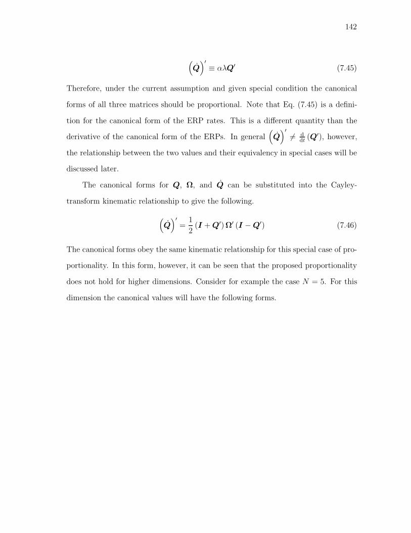
142

(Q)′

≡ αλQ′ (7.45)

Therefore, under the current assumption and given special condition the canonical

forms of all three matrices should be proportional. Note that Eq. (7.45) is a defini-

tion for the canonical form of the ERP rates. This is a different quantity than the

derivative of the canonical form of the ERPs. In general(Q)′

= ddt

(Q′), however,

the relationship between the two values and their equivalency in special cases will be

discussed later.

The canonical forms for Q, Ω, and Q can be substituted into the Cayley-

transform kinematic relationship to give the following.

(Q)′

=1

2(I + Q′)Ω′ (I − Q′) (7.46)

The canonical forms obey the same kinematic relationship for this special case of pro-

portionality. In this form, however, it can be seen that the proposed proportionality

does not hold for higher dimensions. Consider for example the case N = 5. For this

dimension the canonical values will have the following forms.

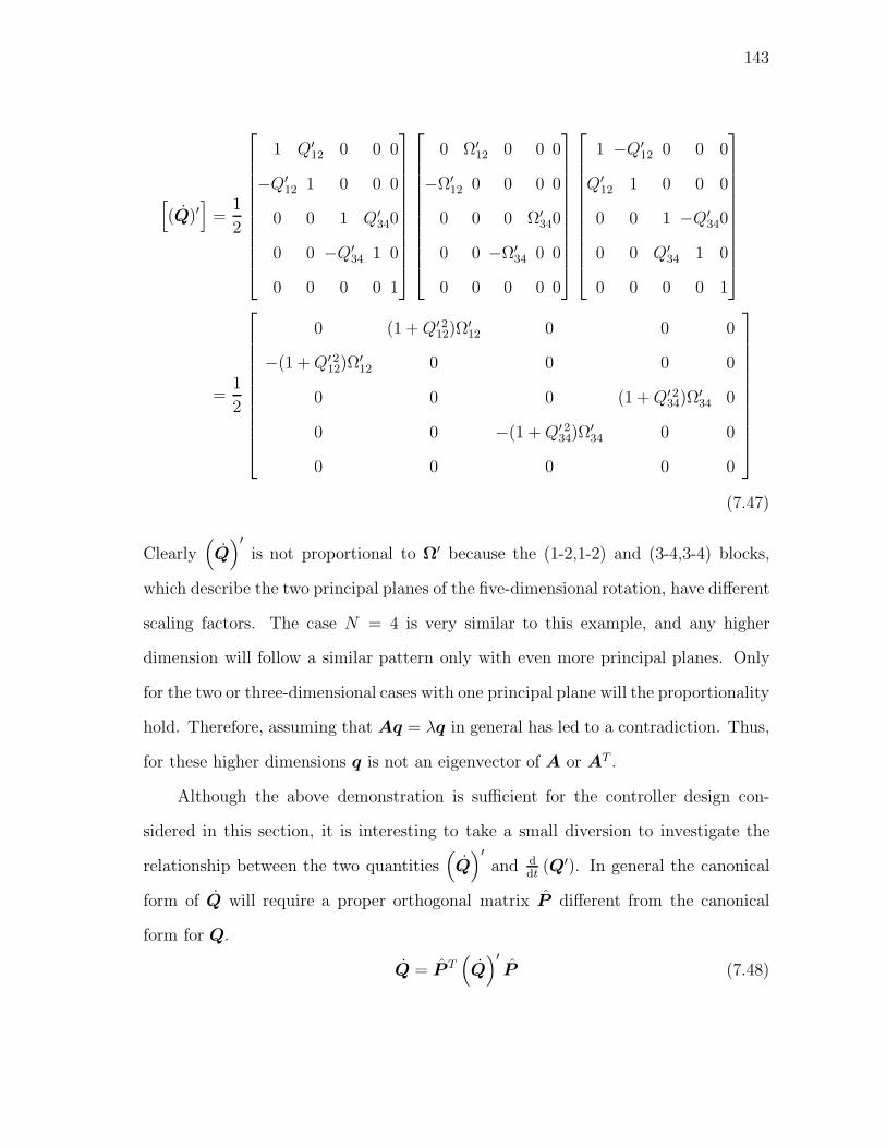
143

[(Q)′

]=

1

2

⎡⎢⎢⎢⎢⎢⎢⎢⎢⎢⎢⎣

1 Q′12 0 0 0

−Q′12 1 0 0 0

0 0 1 Q′340

0 0 −Q′34 1 0

0 0 0 0 1

⎤⎥⎥⎥⎥⎥⎥⎥⎥⎥⎥⎦

⎡⎢⎢⎢⎢⎢⎢⎢⎢⎢⎢⎣

0 Ω′12 0 0 0

−Ω′12 0 0 0 0

0 0 0 Ω′340

0 0 −Ω′34 0 0

0 0 0 0 0

⎤⎥⎥⎥⎥⎥⎥⎥⎥⎥⎥⎦

⎡⎢⎢⎢⎢⎢⎢⎢⎢⎢⎢⎣

1 −Q′12 0 0 0

Q′12 1 0 0 0

0 0 1 −Q′340

0 0 Q′34 1 0

0 0 0 0 1

⎤⎥⎥⎥⎥⎥⎥⎥⎥⎥⎥⎦

=1

2

⎡⎢⎢⎢⎢⎢⎢⎢⎢⎢⎢⎣

0 (1 +Q′ 212)Ω

′12 0 0 0

−(1 +Q′ 212)Ω

′12 0 0 0 0

0 0 0 (1 +Q′ 234)Ω

′34 0

0 0 −(1 +Q′ 234)Ω

′34 0 0

0 0 0 0 0

⎤⎥⎥⎥⎥⎥⎥⎥⎥⎥⎥⎦(7.47)

Clearly(Q)′

is not proportional to Ω′ because the (1-2,1-2) and (3-4,3-4) blocks,

which describe the two principal planes of the five-dimensional rotation, have different

scaling factors. The case N = 4 is very similar to this example, and any higher

dimension will follow a similar pattern only with even more principal planes. Only

for the two or three-dimensional cases with one principal plane will the proportionality

hold. Therefore, assuming that Aq = λq in general has led to a contradiction. Thus,

for these higher dimensions q is not an eigenvector of A or AT .

Although the above demonstration is sufficient for the controller design con-

sidered in this section, it is interesting to take a small diversion to investigate the

relationship between the two quantities(Q)′

and ddt

(Q′). In general the canonical

form of Q will require a proper orthogonal matrix P different from the canonical

form for Q.

Q = P T(Q)′

P (7.48)

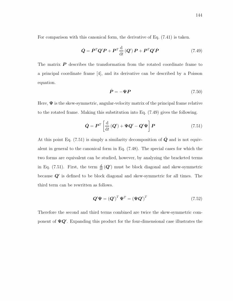
144

For comparison with this canonical form, the derivative of Eq. (7.41) is taken.

Q = P TQ′P + P T d

dt(Q′) P + P TQ′P (7.49)

The matrix P describes the transformation from the rotated coordinate frame to

a principal coordinate frame [4], and its derivative can be described by a Poisson

equation.

P = −ΨP (7.50)

Here, Ψ is the skew-symmetric, angular-velocity matrix of the principal frame relative

to the rotated frame. Making this substitution into Eq. (7.49) gives the following.

Q = P T

[d

dt(Q′) + ΨQ′ − Q′Ψ

]P (7.51)

At this point Eq. (7.51) is simply a similarity decomposition of Q and is not equiv-

alent in general to the canonical form in Eq. (7.48). The special cases for which the

two forms are equivalent can be studied, however, by analyzing the bracketed terms

in Eq. (7.51). First, the term ddt

(Q′) must be block diagonal and skew-symmetric

because Q′ is defined to be block diagonal and skew-symmetric for all times. The

third term can be rewritten as follows.

Q′Ψ = (Q′)TΨT = (ΨQ′)T

(7.52)

Therefore the second and third terms combined are twice the skew-symmetric com-

ponent of ΨQ′. Expanding this product for the four-dimensional case illustrates the

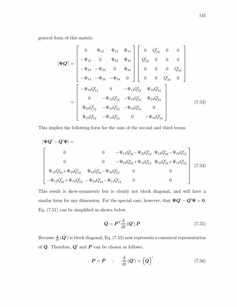
145

general form of this matrix.

[ΨQ′] =

⎡⎢⎢⎢⎢⎢⎢⎢⎣

0 Ψ12 Ψ13 Ψ14

−Ψ12 0 Ψ23 Ψ24

−Ψ13 −Ψ23 0 Ψ34

−Ψ14 −Ψ24 −Ψ34 0

⎤⎥⎥⎥⎥⎥⎥⎥⎦

⎡⎢⎢⎢⎢⎢⎢⎢⎣

0 Q′12 0 0

Q′12 0 0 0

0 0 0 Q′34

0 0 Q′34 0

⎤⎥⎥⎥⎥⎥⎥⎥⎦

=

⎡⎢⎢⎢⎢⎢⎢⎢⎣

−Ψ12Q′12 0 −Ψ14Q

′34 Ψ13Q

′34

0 −Ψ12Q′12 −Ψ24Q

′34 Ψ23Q

′34

Ψ23Q′12 −Ψ13Q

′12 −Ψ34Q

′34 0

Ψ24Q′12 −Ψ14Q

′12 0 −Ψ34Q

′34

⎤⎥⎥⎥⎥⎥⎥⎥⎦(7.53)

This implies the following form for the sum of the second and third terms.

[ΨQ′ − Q′Ψ] =⎡⎢⎢⎢⎢⎢⎢⎢⎣

0 0 −Ψ14Q′34−Ψ23Q

′12 Ψ13Q

′34−Ψ24Q

′12

0 0 −Ψ24Q′34+Ψ13Q

′12 Ψ23Q

′34+Ψ14Q

′12

Ψ14Q′34+Ψ23Q

′12 Ψ24Q

′34−Ψ24Q

′12 0 0

−Ψ13Q′34+Ψ13Q

′12 −Ψ23Q

′34−Ψ14Q

′12 0 0

⎤⎥⎥⎥⎥⎥⎥⎥⎦(7.54)

This result is skew-symmetric but is clearly not block diagonal, and will have a

similar form for any dimension. For the special case, however, that ΨQ′ −Q′Ψ = 0,

Eq. (7.51) can be simplified as shown below.

Q = P T d

dt(Q′) P (7.55)

Because ddt

(Q′) is block diagonal, Eq. (7.55) now represents a canonical representation

of Q. Therefore, Q′ and P can be chosen as follows.

P = P ;d

dt(Q′) =

(Q)′

(7.56)

146

Conversely, for motions prescribed such that Q and Q are brought into canonical

form by the same transformation matrix P = P , the following must be true.

ΨQ′ − Q′Ψ = 0 ;d

dt(Q′) =

(Q)′

(7.57)

Therefore, for these special motions, which can be described by either specifying Ψ

and Q′ or P and P , differentiation and the canonical transformation of the ERPs

are commutative.

Returning to the topic of controller design, because the eigenvalue property of

AT does not extend to N -dimensions, the Lyapunov function used by Tsiotras can

not be utilized to develop a linear feedback controller for N -dimensional rigid bodies.

This function, V = 12ωiJijωj + ln(1 + qiqi), and others can be used, however, to

develop globally asymptotically stable nonlinear feedback controllers. Applying the

work/energy-rate expression from the previous section gives the following for the

derivative of the Lyapunov function.

V = ωif(ω)i +

ddt

(1 + qiqi)

1 + qiqi=

1

2ΩjkF

(ω)jk +

ddt

(1 + 1

2QjkQjk

)1 + qiqi

=1

2ΩjkF

(ω)jk +

QjkQjk

1 + qiqi=

1

2ΩjkF

(ω)jk +

Qjk (δjr +Qjr)Ωrs (δsk −Qsk)

2(1 + qiqi)

=1

2ΩjkF

(ω)jk +

(Qrk +QjkQjr)Ωrs (δsk −Qsk)

2(1 + qiqi)

=1

2ΩjkF

(ω)jk +

Ωrs (Qrs −QrkQsk +QjsQjr −QjkQjrQsk)

2(1 + qiqi)

=1

2ΩjkF

(ω)jk +

Ωrs (Qrs −QrjQjkQks)

2(1 + qiqi)(7.58)

The following nonlinear feedback controller will set the Lyapunov function derivative

to be negative semi-definite.

F(ω)jk = −Ωjk − (Qjk −QjmQmnQnk)

1 + qiqi(7.59)

147

Here, the first term of the control law is referred to as a stabilization term, and the

second term is referred to as a regulation term. For three-dimensions this expression

can be simplified by extracting a factor of Q from the numerator of the regulation

term leading to cancelation of the denominator. This cancelation, however, uses the

property that q is an eigenvector of AT , which does not hold in general as has just

been shown. For general N -dimensions no further simplifications can be made.

Another more typical Lyapunov function that can be used is the sum of kinetic

energy and a quadratic product of the coordinates.

V =1

2ωiJijωj + qiqi =

1

2ωiJijωj +

1

2QjkQjk (7.60)

The derivative of this function is shown below.

V =1

2ΩlmF

(ω)lm +QjkQjk =

1

2ΩlmF

(ω)lm +

1

2Qjk (δjl +Qjl) Ωlm (δmk −Qmk)

=1

2Ωlm

(F

(ω)lm + (Qlk +QjkQjl) (δmk −Qmk)

)=

1

2Ωlm

(F

(ω)lm +Qlm −QlkQmk +QjmQjl −QjkQjlQmk

)=

1

2Ωlm

(F

(ω)lm +Qlm −QjkQjlQmk

)(7.61)

For global asymptotic stability the control is chosen as follows.

F(ω)lm = −Ωlm −Qlm +QljQjkQkm (7.62)

This can also be expressed in matrix notation.

F (ω) = −Ω− Q + QQQ = −Ω − Q (I −QQ) = −Ω − Q(I + QT Q

)(7.63)

Again, this controller contains both stabilization and regulation terms. In two follow-

ing sections these terms will be further analyzed. The regulation terms for both of the

controllers developed in this section will be shown to optimize certain cost functions

148

for control of the kinematic equations. Additionally, numerical simulation will be

used to compare the stabilization behavior of Cayley quasi-velocity feedback against

generalized-velocity feedback and another choice of quasi-velocity feedback. First,

however, a second set of quasi velocities is developed that allows globally asymptoti-

cally stable linear feedback.

F. Quasi Velocities for Linear Feedback

In Section C several special properties of the angular-velocity/Rodrigues-parameter

kinematics were discussed that led to a proof for global asymptotic stability of linear

feedback. Those kinematics are described by the transformation matrix A, whose

elements are repeated here for convenience.

Aim =1


Sections D and E presented an attempt to extend that proof to M-DOF physical

systems by recognizing that the three-dimensional motion variables are simply a spe-

cial case of the Cayley form. That approach used a general form of Eq. (7.64) to

describe N -dimensional rotations. It was found, however, that the complexity of

the N -dimensional kinematics produced difficulty in extending the proof. This sec-

tion presents an alternative approach to extending that proof by defining a new set of

quasi velocities. Instead of extending the rotational kinematics of Eq. (7.64) to higher

dimensions like the Cayley quasi velocities, the new quasi velocities are defined by

simply modifying the functional form of Eq. (7.64).

To do this a newM×M transformation matrix A will be defined. Two difficulties

exist, however, in directly extending the functional form of Eq. (7.64) to any M-DOF

system. Both are directly related to the second term, Qim. First Q can only be

149

formed for certain values of M , and second Q is N ×N in general, not M ×M . This

suggests the following mapping to define a new set of quasi velocities u.

q = Au ; u = Bq (7.65)

Aim =1

2(δim + qiqm) (7.66)

This set of quasi velocities can be applied to a general system with any number of

generalized coordinates. For Eqs. (7.65) and (7.66) to constitute a valid quasi-velocity

definition, however, the inverse of A (i.e., B) must exist. In vector/matrix notation

2A is equal to I + qqT , and the eigenvalues of 2A are found by adding one to the

eigenvalues of qqT . To show that A is nonsingular it simply needs to be demonstrated

that negative one can not be an eigenvalue of qqT . If it is assumed that qqT does have

an eigenvalue of negative one and a corresponding eigenvector e, then the following

eigenproblem can be considered.

qqTe =(qT e

)q = −e (7.67)

This implies that e must be proportional to q.

e = αq (7.68)

α(qTq

)q = −αq (7.69)

Thus assuming that qqT has an eigenvalue of negative one has led to the contradiction

qT q = −1. Therefore, A is nonsingular, and u is a valid set of quasi velocities.

Before continuing with the new quasi velocities, it is worth revisiting the work/

energy-rate expression for general quasi velocities. For natural systems the work/

energy-rate expression with respect to the generalized velocities can be expressed as

T = qT f . Considering a set of quasi velocities as defined by Eq. (7.65), Poincare’s

150

equations define the quasi forces.

f (u) = AT f ; f = BT f (u) (7.70)

Equations (7.65) and (7.70) can be used to write the work/energy-rate expression for

any set of quasi velocities, once and for all.

T = qT f = uTAT BT f (u) = uTf (u) (7.71)

Of course this expression is consistent with the work/energy-rate expression found

for N -dimensional rotations in Section D.

Returning to the particular set of quasi velocities defined by Eq. (7.66), linear

feedback of q and u can be proven to be globally asymptotically stable. Consider

again the Lyapunov function defined by Tsiotras for the sum of the kinetic energy

and a fictitious potential energy, where J (q) is the mass matrix associated with u.

V =1

2uiJijuj + ln (1 + qiqi) (7.72)

The time derivative is given by the following.

V = uif(u)i +

2qiqi

1 + qjqj= uif

(u)i +

2qiAimum

1 + qjqj(7.73)

Due to the choice of A, however, q is now an eigenvector of AT for any value of M .

qiAim =1

2(δimqi + qiqmqi) =

1

2(qm + qiqiqm) =

1

2(1 + qiqi) qm ≡ λqm (7.74)

Therefore, the time derivative of the Lyapunov function can be simplified.

V = uif(u)i + qiui (7.75)

If the control elements, f(u)i , are chosen to make Eq. (7.24) negative definite, then

the system will be globally asymptotically stable. This can be done in the following

151

fashion.

V = uif(u)i + qiui ≡ −uiui (7.76)

f(u)i = −ui − qi (7.77)

Equation (7.77) demonstrates that linear feedback of the generalized coordinates and

the new quasi velocities, defined by Eqs. (7.65) and (7.66), will provide global asymp-

totic stability for any system.

G. Optimality Results for Regulation Terms

In the previous sections the control of a complete system, both dynamic and kinematic

equations, using quasi velocities was discussed. In this section the control of only the

kinematic equations, returning to the Cayley quasi velocities, will be considered. This

approach treats the Cayley quasi velocities as control variables used to control the

generalized coordinates. The cost functions optimized by feedback laws with the form

of the regulation terms from the previous section will be developed.

First for notational convenience the vector q is defined as the generating vector

of the skew-symmetric, cubic product QQQ.

qa =1

2χa

mlQmkQkjQjl (7.78)

The minimization of the following cost function subject to the kinematic equations

will be considered.

J =1

2

∫ ∞

0

[k2 (q − q)T (q − q) + ωTω

]dt (7.79)

q = Aω (7.80)

152

Introducing the costates λ, the Hamiltonian is written below.

H (q,ω,λ) =1

2k2 (q − q)T (q − q) +

1

2ωTω + λT Aω (7.81)

Next, the following three conditions on the optimal trajectory are imposed.

H = 0 ;∂H

∂ω= ω + AT ∂V

∂q= 0 ; λ =

∂V

∂q(7.82)

Here, V is the unknown optimal-cost function. These conditions are substituted into

Eq. (7.81) to develop the Hamilton-Jacobi-Bellman equation for this problem.

k2 (q − q)T (q − q) −(∂V

∂q

)T

AAT ∂V

∂q= 0 (7.83)

Now, the candidate optimal-cost function V = kqT q is considered. The optimal

control implied by this candidate solution is found using Eq. (7.82).

ω = −AT ∂V

∂q= −2kAT q (7.84)

This is evaluated using Eqs. (7.36) and (7.37).

Aimqi =1

2

(δimqi − 1

2χi

vpχmklQvkQlpqi

)=

1

2

(qm − 1

2χm

klQvkQlpQvp

)=

1

2

(qm − 1

2χm

klQkvQvpQpl

)=

1

2(qm − qm) (7.85)

Equations (7.84) and (7.85) can be substituted into Eq. (7.83) to show that the

candidate optimal-cost function is indeed a solution of the Hamilton-Jacobi-Bellman

equation. The final form of the optimal control is shown below.

ω = −k (q − q) (7.86)

153

Notice that this feedback controller is equal to the regulation term of the second

controller from Section E, and the optimal-cost function is equal to the regulation

term of the Lyapunov function corresponding to that controller.

A second optimal-control problem of the kinematic equations can be considered

using the following cost function.

J =1

2

∫ ∞

0

[k2 (q − q)T (q − q)

(1 + qT q)2 + ωTω

]dt (7.87)

The corresponding Hamiltonian is shown below.

H (q,ω,λ) =1

2k2 (q − q)T (q − q)

(1 + qTq)2 +1

2ωTω + λT Aω (7.88)

For this problem the optimality conditions are identical to Eq. (7.82) and can be

expanded to give the following Hamilton-Jacobi-Bellman equation.

k2 (q − q)T

(q − q)

(1 + qTq)2 −(∂V

∂q

)T

AAT ∂V

∂q= 0 (7.89)

For this problem the candidate optimal-cost function V = k ln(1 + qTq

)is consid-

ered. To demonstrate that this function satisfies Eq. (7.89), first, the gradient of V

is taken.

∂V

∂q=

2kq

1 + qTq(7.90)

AT ∂V

∂q=

2kAT q

1 + qT q=k (q − q)

1 + qTq(7.91)

Clearly the candidate optimal-cost function is a solution of the Hamilton-Jacobi-

Bellman equation. The optimal control implied by the second of Eqs. (7.82) is shown

below.

ω = −k (q − q)

1 + qTq(7.92)

154

Again, notice that this control is equal to the regulation term of the first controller

from Section E, and the optimal-cost function is the regulation term of the associated

Lyapunov function.

H. Stabilization Using Velocity Feedback

Whereas the previous section analyzed the regulation terms of the Cayley quasi ve-

locity feedback controllers and Lyapunov functions, this section focuses on the stabi-

lization terms. In this section the kinetic energy alone, shown in Eq. (7.29), is used

as a Lyapunov function. In a previous section the derivative of the kinetic energy

was found to be the work done by the quasi forces associated with the Cayley quasi

velocities.

T = ωTf (ω) (7.93)

The generalized forces can be selected to make this derivative negative semi-definite.

f (ω) = −Dω (7.94)

Here, D is a symmetric, positive-definite matrix. For simplicity, in previous sections

D was chosen to be the identity matrix.

f (ω) = −ω (7.95)

f = −BTω = −BTBq (7.96)

Another choice that will be investigated in this section is D = P ω (AA)T (AA),

which is positive definite because A is full rank, and where P ω is a control gain. This

choice leads to the following controller.

f (ω) = −Pω (AA)T (AA) ω (7.97)

155

f = −PωBT (AA)T (AA)ω = −PωAT Aq (7.98)

The controller in Eq. (7.98) is referred to as the ω control law. The performance

of this controller will be compared to two other feedback controllers: one using the

generalized velocities and one designed by Schaub and Junkins [47] using a different

set of quasi velocities. The controller designed by Schaub and Junkins is summarized

below.

Using a spectral decomposition with square-root factorization of the eigenvalue

matrix, the system mass matrix can be written as the following.

M = CTSTSC (7.99)

Here, C is proper orthogonal, and S is diagonal. The eigenfactor quasi velocities are

defined as η = SCq and can be used to rewrite the kinetic energy.

T =1

2ηTη (7.100)

Through the development of the dynamic equations in terms of η, Schaub and Junkins

showed that the derivative of the kinetic energy is equal to the work done by the quasi

forces associated with the eigenfactor quasi velocities.

T = ηT f (η) (7.101)

From this a globally asymptotically stable control law is chosen to be the following.

f (η) = −P ηη (7.102)

This corresponds to the following controller for the generalized forces in terms of the

generalized velocities, and is referred to as the η control law.

f = −P ηMq (7.103)

156

In addition to the eigenfactor and Cayley quasi-velocity controllers, a conventional

controller using the generalized velocities was implemented. This is developed using

the kinetic energy written as T = 12qMq, and results in the following q control law.

f = −P qq (7.104)

Again following Schaub and Junkins [47], the controllers in Eqs. (7.98), (7.103),

and (7.104) were applied to a planar three-link manipulator system. The generalized

coordinates of the system are [q] = [ θ1 θ2 θ3 ]T and are the absolute angles of each

joint. The generalized forces are related to the motor torques acting at each joint.

The system mass matrix was given by Schaub and Junkins.

[M ] =

⎡⎢⎢⎢⎢⎣(m1 +m2 +m3) l

21 (m2+m3) l1l2 cos (θ2−θ1) m3l1l3 cos (θ3 − θ1)

(m2+m3) l1l2 cos (θ2−θ1) (m2 +m3) l22 m3l2l3 cos (θ3 − θ2)

m3l1l3 cos (θ3 − θ1) m3l2l3 cos (θ3 − θ2) m3l23

⎤⎥⎥⎥⎥⎦(7.105)

Here, m1, m2, and m3 are the masses of point masses located at the tip of each link,

and l1, l2, and l3 are the lengths of each link.

Simulations were performed using initial states of [q (0)] = [ 93 −110 −73 ]T

degrees. The initial velocities were chosen to be [q (0)] = [ −90 30 0 ]T degrees/

second. The values m1, m2, m3, l1, l2, and l3 were set to one. The control gains

were chosen for each controller such that the absolute control effort encountered was

equal. The values P q = 1.1, P η = 0.59, and Pω = 0.38 were chosen. The numerical

integration was performed using a fourth and fifth order Runge-Kutta method and a

simulation duration of 15 seconds.

The results from the simulation are shown in Figs. 14 and 15. The plot of the

control effort, the magnitude of f , on a logarithmic scale shows that each of the

control laws goes through a peak in the first few seconds, but then begin to drop off

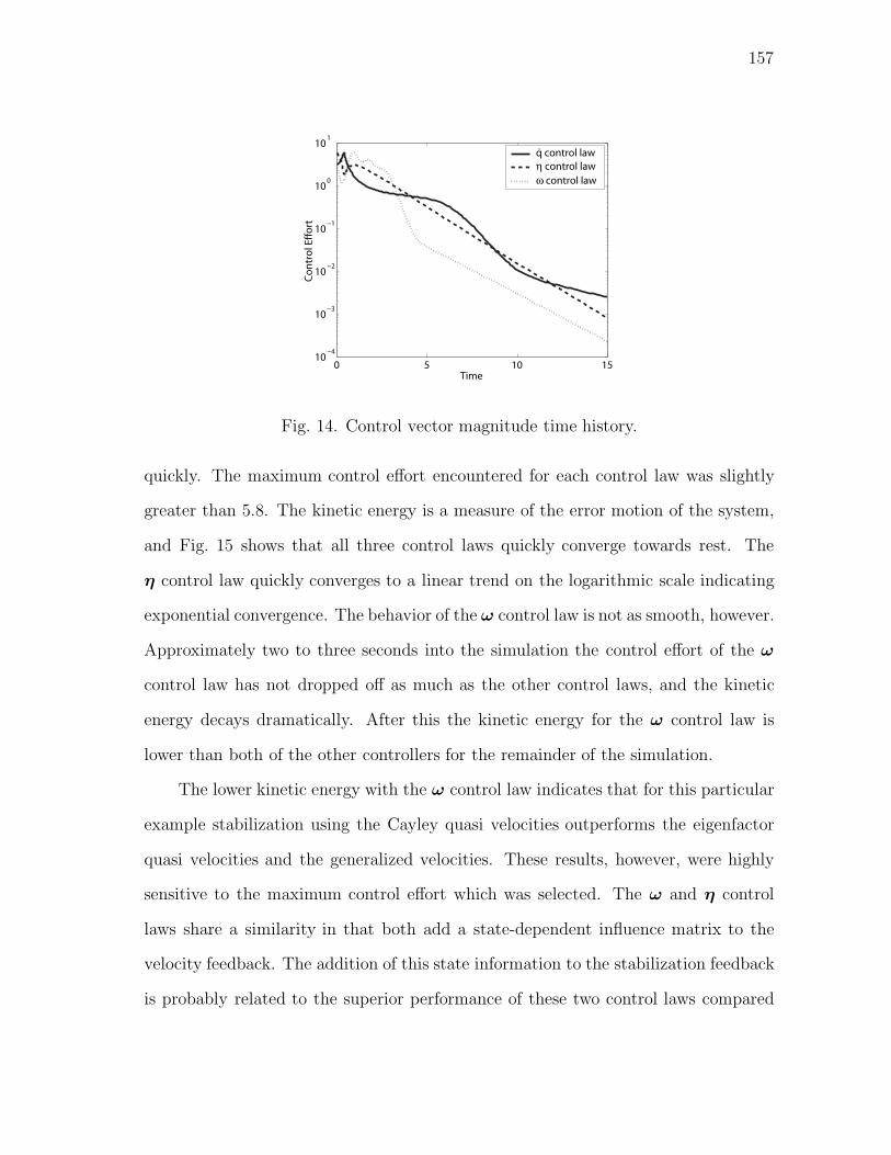
157

0 5 10 1510

−4

10−3

10−2

10−1

100

101

Time

Con

trol

Eff

ort

q control lawη control lawω control law

.

Fig. 14. Control vector magnitude time history.

quickly. The maximum control effort encountered for each control law was slightly

greater than 5.8. The kinetic energy is a measure of the error motion of the system,

and Fig. 15 shows that all three control laws quickly converge towards rest. The

η control law quickly converges to a linear trend on the logarithmic scale indicating

exponential convergence. The behavior of the ω control law is not as smooth, however.

Approximately two to three seconds into the simulation the control effort of the ω

control law has not dropped off as much as the other control laws, and the kinetic

energy decays dramatically. After this the kinetic energy for the ω control law is

lower than both of the other controllers for the remainder of the simulation.

The lower kinetic energy with the ω control law indicates that for this particular

example stabilization using the Cayley quasi velocities outperforms the eigenfactor

quasi velocities and the generalized velocities. These results, however, were highly

sensitive to the maximum control effort which was selected. The ω and η control

laws share a similarity in that both add a state-dependent influence matrix to the

velocity feedback. The addition of this state information to the stabilization feedback

is probably related to the superior performance of these two control laws compared

158

0 5 10 1510

−8

10−6

10−4

10−2

100

102

Time

Kine

tic E

nerg

y

q control lawη control lawω control law

.

Fig. 15. Kinetic energy time history.

to the generalized-velocity feedback. For the η control law this influence matrix is

the mass matrix, M , and is dependent on knowledge of system parameters. The ω

control law, however, uses ATA which is only dependent on kinematic definitions and

is not susceptible to system uncertainty.

I. Conclusion

This chapter has demonstrated a novel approach for the design of feedback controllers

for natural mechanical systems. This approach is enabled by the Cayley form, which

allows systems to be represented as N -dimensional rigid bodies. Several examples

of feedback controllers were developed by extending spacecraft attitude controllers

to N -dimensional rotations. It was found, however, that the complications of N -

dimensional kinematics (i.e., multiple principal planes) clouded, or perhaps destroyed,

some of the elegance of the three-dimensional results.

The controllers developed in this chapter were further analyzed for optimal-

ity and performance. First, the cost functions optimized by the regulation terms

159

were developed. Second, numerical simulation was used to compare the stabilization

performance of Cayley quasi-velocity feedback, eigenfactor quasi-velocity feedback,

and generalized-velocity feedback. Results were presented for one example showing

superior performance for Cayley quasi-velocity feedback. Of course, this does not

demonstrate superiority in any global sense (nor is it believed to exist). Such global

demonstrations of performance are a very difficult problem in nonlinear control.

The results that are presented, however, do provide an example of the significance

of control coupling. A disadvantage of the Cayley form from a dynamics perspective is

that it produces coupling in the equations of motion between coordinates that might

otherwise be uncoupled. From a control perspective, however, having a controller that

reflects the coupling that already exists in the dynamics can be advantageous. Both

the Cayley and eigenfactor quasi-velocity feedbacks represent a coupling between each

control and every velocity. The generalized-velocity feedback, however, matches the

controls to the velocities in a one-to-one fashion, out of simplicity, that does not reflect

the dynamics. Whereas this simplicity is attractive in itself, it does not guarantee

superior performance.

160

CHAPTER VIII

NONLINEARITY INDEX OF THE CAYLEY FORM

A. Introduction

The previous two chapters presented applications of the Cayley form for developing

representations of system dynamics and for designing feedback controllers. In both

of these chapters it was significant that the Cayley form produces coupled system

representations. In Chapter VI it was noted that the resulting equations of motion

from the Cayley form can be more complicated than alternative methods that result

in decoupled equations of motion, and in Chapter VII numerical-simulation results

indicated that designing controllers based on coupled representations can in some

cases result in superior performance. These issues motivate a desire to analyze the

Cayley form to quantitatively measure these properties related to complexity and

coupling.

The Cayley form, of course, is just one example of the generally infinite possi-

bilities for representing dynamic systems. Due to the broad variety of system repre-

sentations, the idea of comparing different representations of a physical system (or

indeed, representations of different physical systems) is not a new one. Methods have

been developed to analyze and compare system representations. One of these is the

nonlinearity index developed by Junkins [48, 49]. In this chapter the nonlinearity

index of the Cayley form and two alternative representations will be computed for a

sample problem. First, however, the definition of the nonlinearity index is reviewed.

161

B. Nonlinearity Index

As mentioned, generally infinite possibilities exist for coordinate choices to represent

any given physical system. Much of the history of analytical mechanics has spawned

from the development of new coordinate choices. Several issues effect the choice of a

particular coordinate system. A typical approach defines one set of position-level co-

ordinates to describe the configuration of the system and a second set of velocity-level

coordinates to describe the evolution of the system. One issue that effects the choice

of position-level coordinates is the presence of singularities, e.g., configurations which

can not be described by a particular set of coordinates or configurations for which the

coordinates are undefined. A classic example of this is the variety of popular choices

for representing the orientation of a rigid body. Choices for velocity-level coordinates

(such as the Cayley form) generally provide canonical representations for the dynam-

ics of broad classes of problems. Examples of this are the conjugate momenta and

quasi velocities. Of course, alternatives to the split position and velocity-level coor-

dinates also exist, such as the classic orbital elements that describe both the position

and velocity of a spacecraft in a single set of variables.

Along with the issues of singularities and canonical representation, another issue

related to coordinate choice is the linearity or nonlinearity of the resulting dynamical

system. Of course, linear equations are desirable; however, it is difficult to make

general comparisons of nonlinear dynamical systems. One approach to do this is the

nonlinearity index developed by Junkins, which provides a measure for the nonlinear-

ity of a dynamical system and a particular initial condition. Consider the following

dynamical system.

x = f (t,x) ; x (t0) = x0 (8.1)

162

The first-order sensitivity of the trajectory to the initial conditions are described by

the state-transition matrix.

Φ (t, t0) =∂x (t)

∂x (t0)(8.2)

The state-transition matrix satisfies the following differential equation.

Φ (t, t0) = FΦ (t, t0) ; F =∂f (t,x)

∂x (t); Φ (t0, t0) = I (8.3)

Of course, for a linear system the Jacobian matrix F is constant. Therefore, for

linear systems Φ (t, t0) is independent of the initial condition x (t0). In other words,

the state-transition matrix Φ (t, t0) evaluated along a nominal trajectory with initial

condition x (t0) will be exactly equal to the state-transition matrix Φ (t, t0) evaluated

along any neighboring trajectory with initial condition x (t0). This suggests using

the magnitude of the difference between state-transition matrices evaluated along

neighboring trajectories as a measure of nonlinearity. In particular the following

nonlinearity index was suggested by Junkins [48, 49].

ν (t, t0) ≡ supi=1...n

∥∥Φi (t, t0) − Φ (t, t0)∥∥∥∥Φ (t, t0)

∥∥ (8.4)

Here, Φi (t, t0) is the state-transition matrix evaluated along the trajectory corre-

sponding to the ith initial condition from a family of n neighboring initial conditions.

The selection of the neighboring initial conditions is clearly an important issue

in computing the nonlinearity index for any system and nominal initial condition.

In the following study, this selection was performed using a method suggested by

Junkins and Singla of populating an M-dimensional sphere surrounding the nominal

initial condition in state space [49]. The initial conditions are found by distributing

points approximately uniformly on the M-dimensional sphere using an optimization

process. This is done by considering the points as identical attracting particles on

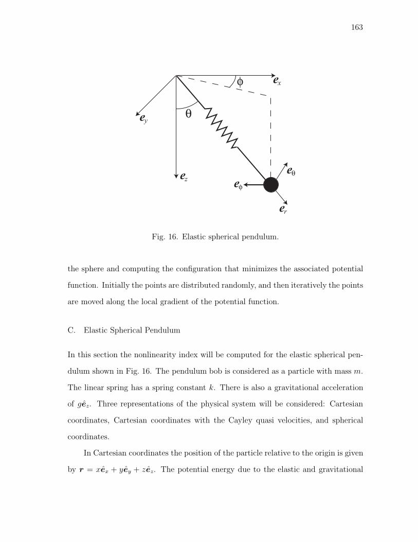
163

θ

φ

Fig. 16. Elastic spherical pendulum.

the sphere and computing the configuration that minimizes the associated potential

function. Initially the points are distributed randomly, and then iteratively the points

are moved along the local gradient of the potential function.

C. Elastic Spherical Pendulum

In this section the nonlinearity index will be computed for the elastic spherical pen-

dulum shown in Fig. 16. The pendulum bob is considered as a particle with mass m.

The linear spring has a spring constant k. There is also a gravitational acceleration

of gez. Three representations of the physical system will be considered: Cartesian

coordinates, Cartesian coordinates with the Cayley quasi velocities, and spherical

coordinates.

In Cartesian coordinates the position of the particle relative to the origin is given

by r = xex + yey + zez. The potential energy due to the elastic and gravitational

164

potentials is given by V = k(x2+y2+z2)/2−mgz. From these the following decoupled,

linear equations of motion are found.

mx+ kx = 0

my + ky = 0 (8.5)

mz + kz −mg = 0

In spherical coordinates the position vector is given by r = rer, and the angular

velocity of the body-fixed frame is given by ωB/I = φez + θeφ. The potential energy

is given by V = kr2/2 −mgr cos(θ). Unlike the Cartesian coordinates, the equations

of motion for the spherical coordinates are coupled and nonlinear.

r = rθ2 + rφ2 sin2 (θ) − k

mr + g cos (θ)

θ = φ2 sin (θ) cos (θ) − 2rθ

r− g

rsin (θ) (8.6)

φ = −2rφ

r− 2φθ

cos (θ)

sin (θ)

In deriving these equations, it is found that φ is a cyclic coordinate and the motion

constant hz = r2φ sin2 (θ) exists. This constant is the vertical component of the

angular momentum about the origin.

The final representation of the elastic spherical pendulum that will be considered

is Cartesian coordinates in the Cayley form. This uses the Cartesian coordinates for

generalized coordinates, [q] = [x y z]T , and the associated Cayley quasi velocities,

[ω] = [ω1 ω2 ω3]T , for velocity-level coordinates. The Cayley quasi velocities for this

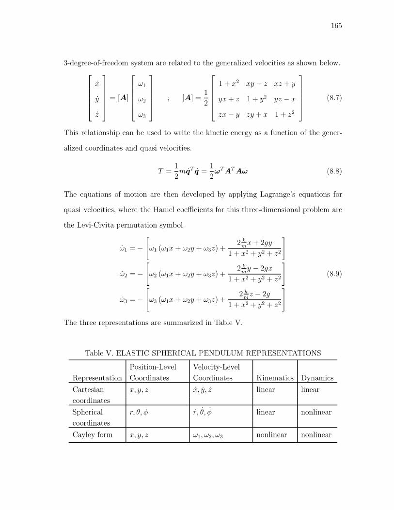
165

3-degree-of-freedom system are related to the generalized velocities as shown below.⎡⎢⎢⎢⎢⎣x

y

z

⎤⎥⎥⎥⎥⎦ = [A]

⎡⎢⎢⎢⎢⎣ω1

ω2

ω3

⎤⎥⎥⎥⎥⎦ ; [A] =1

2

⎡⎢⎢⎢⎢⎣1 + x2 xy − z xz + y

yx+ z 1 + y2 yz − x

zx− y zy + x 1 + z2

⎤⎥⎥⎥⎥⎦ (8.7)

This relationship can be used to write the kinetic energy as a function of the gener-

alized coordinates and quasi velocities.

T =1

2mqT q =

1

2ωTAT Aω (8.8)

The equations of motion are then developed by applying Lagrange’s equations for

quasi velocities, where the Hamel coefficients for this three-dimensional problem are

the Levi-Civita permutation symbol.

ω1 = −[ω1 (ω1x+ ω2y + ω3z) +

2 kmx+ 2gy

1 + x2 + y2 + z2

]

ω2 = −[ω2 (ω1x+ ω2y + ω3z) +

2 kmy − 2gx

1 + x2 + y2 + z2

](8.9)

ω3 = −[ω3 (ω1x+ ω2y + ω3z) +

2 kmz − 2g

1 + x2 + y2 + z2

]

The three representations are summarized in Table V.

Table V. ELASTIC SPHERICAL PENDULUM REPRESENTATIONS

Position-Level Velocity-Level

Representation Coordinates Coordinates Kinematics Dynamics

Cartesian x, y, z x, y, z linear linear

coordinates

Spherical r, θ, φ r, θ, φ linear nonlinear

coordinates

Cayley form x, y, z ω1, ω2, ω3 nonlinear nonlinear

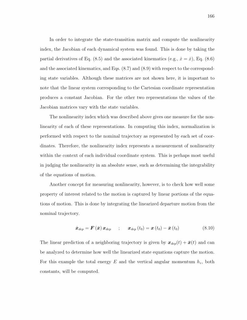
166

In order to integrate the state-transition matrix and compute the nonlinearity

index, the Jacobian of each dynamical system was found. This is done by taking the

partial derivatives of Eq. (8.5) and the associated kinematics (e.g., x = x), Eq. (8.6)

and the associated kinematics, and Eqs. (8.7) and (8.9) with respect to the correspond-

ing state variables. Although these matrices are not shown here, it is important to

note that the linear system corresponding to the Cartesian coordinate representation

produces a constant Jacobian. For the other two representations the values of the

Jacobian matrices vary with the state variables.

The nonlinearity index which was described above gives one measure for the non-

linearity of each of these representations. In computing this index, normalization is

performed with respect to the nominal trajectory as represented by each set of coor-

dinates. Therefore, the nonlinearity index represents a measurement of nonlinearity

within the context of each individual coordinate system. This is perhaps most useful

in judging the nonlinearity in an absolute sense, such as determining the integrability

of the equations of motion.

Another concept for measuring nonlinearity, however, is to check how well some

property of interest related to the motion is captured by linear portions of the equa-

tions of motion. This is done by integrating the linearized departure motion from the

nominal trajectory.

xdep = F (x)xdep ; xdep (t0) = x (t0) − x (t0) (8.10)

The linear prediction of a neighboring trajectory is given by xdep(t) + x(t) and can

be analyzed to determine how well the linearized state equations capture the motion.

For this example the total energy E and the vertical angular momentum hz, both

constants, will be computed.

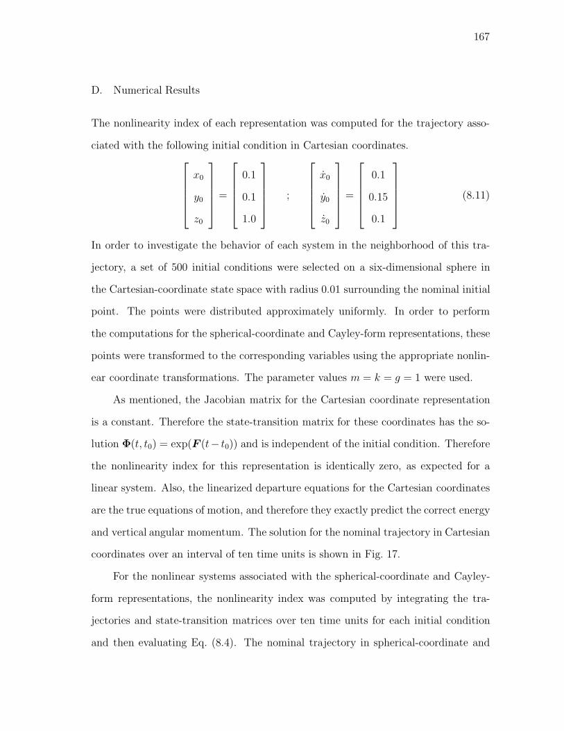
167

D. Numerical Results

The nonlinearity index of each representation was computed for the trajectory asso-

ciated with the following initial condition in Cartesian coordinates.⎡⎢⎢⎢⎢⎣x0

y0

z0

⎤⎥⎥⎥⎥⎦ =

⎡⎢⎢⎢⎢⎣0.1

0.1

1.0

⎤⎥⎥⎥⎥⎦ ;

⎡⎢⎢⎢⎢⎣x0

y0

z0

⎤⎥⎥⎥⎥⎦ =

⎡⎢⎢⎢⎢⎣0.1

0.15

0.1

⎤⎥⎥⎥⎥⎦ (8.11)

In order to investigate the behavior of each system in the neighborhood of this tra-

jectory, a set of 500 initial conditions were selected on a six-dimensional sphere in

the Cartesian-coordinate state space with radius 0.01 surrounding the nominal initial

point. The points were distributed approximately uniformly. In order to perform

the computations for the spherical-coordinate and Cayley-form representations, these

points were transformed to the corresponding variables using the appropriate nonlin-

ear coordinate transformations. The parameter values m = k = g = 1 were used.

As mentioned, the Jacobian matrix for the Cartesian coordinate representation

is a constant. Therefore the state-transition matrix for these coordinates has the so-

lution Φ(t, t0) = exp(F (t− t0)) and is independent of the initial condition. Therefore

the nonlinearity index for this representation is identically zero, as expected for a

linear system. Also, the linearized departure equations for the Cartesian coordinates

are the true equations of motion, and therefore they exactly predict the correct energy

and vertical angular momentum. The solution for the nominal trajectory in Cartesian

coordinates over an interval of ten time units is shown in Fig. 17.

For the nonlinear systems associated with the spherical-coordinate and Cayley-

form representations, the nonlinearity index was computed by integrating the tra-

jectories and state-transition matrices over ten time units for each initial condition

and then evaluating Eq. (8.4). The nominal trajectory in spherical-coordinate and

168

0 2 4 6 8 100.5

0

0.5

1

1.5

Pos

ition

xy

z

0 2 4 6 8 100.2

0.1

0

0.1

0.2

Time

Vel

ocity

x

y

z.

.

.

Fig. 17. Nominal trajectory in Cartesian coordinates.

Cayley-form representations are shown in Figs. 18 and 19. The nonlinearity indices

found for each representation are shown in Figs. 20 and 21. The average value of the

nonlinearity index over the time interval and the maximum value are shown for both

spherical coordinates and the Cayley form in Table VI. These results show much

lower nonlinearity indices for the Cayley form than the spherical coordinates.

In addition to the nonlinearity index, the errors in linear prediction of E and

hz were also computed. The linearized departure equations were integrated using

the same nominal trajectory, set of initial conditions, and parameter values. The

maximum error in E and hz over the set of initial conditions was computed for each

point in time. For the spherical coordinates the errors in these constants are shown

in Fig. 22, and for the Cayley form the errors are shown in Fig. 23. The average

values of the errors over the time interval and the maximum values are shown for

both spherical coordinates and the Cayley form in Table VI. These results show that

the linearized departure equations for the Cayley form perform much better than the

spherical coordinates in predicting the correct values for the constants E and hz.

169

Table VI. NUMERICAL RESULTS FOR NONLINEARITY

Spherical coordinates Cayley form

ν, average 0.4747 0.0114

ν, maximum 6.7956 0.0179

E, average 5.3768 × 10−4 1.1347 × 10−5

E, maximum 8.1235 × 10−3 1.6418 × 10−5

hz, average 2.3004 × 10−4 7.2015 × 10−6

hz, maximum 1.2375 × 10−3 1.2244 × 10−5

0 2 4 6 8 10

0

5

10

Pos

ition

Coo

rds.

r

θ

φ

0 2 4 6 8 10

0

5

10

Time

Vel

ocity

Coo

rds.

r θ

φ.

. .

Fig. 18. Nominal trajectory in spherical coordinates.

170

0 2 4 6 8 10−0.4

−0.3

−0.2

−0.1

0

0.1

0.2

0.3

0.4

Time

Cay

ley

Qua

si V

eloc

ities

ω1

ω2

ω3

Fig. 19. Nominal trajectory for Cayley quasi velocities.

0 2 4 6 8 100

1

2

3

4

5

6

7

Time

Non

linea

rity

Inde

x

Fig. 20. Nonlinearity index for spherical coordinates.

171

0 2 4 6 8 100

0.002

0.004

0.006

0.008

0.01

0.012

0.014

0.016

0.018

Time

Non

linea

rity

Inde

x

Fig. 21. Nonlinearity index for Cayley form.

0 2 4 6 8 100

1

2

3

4

5

6

7

8

9x 10

−3

Time

Err

or

Eh

z

Fig. 22. Linearization error in motion constants for spherical coordinates.

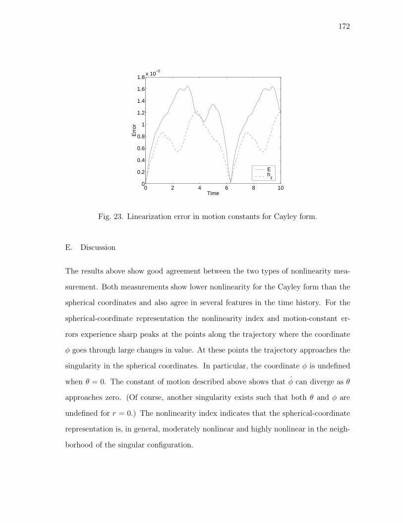
172

0 2 4 6 8 100

0.2

0.4

0.6

0.8

1

1.2

1.4

1.6

1.8x 10

−5

Time

Err

or

Eh

z

Fig. 23. Linearization error in motion constants for Cayley form.

E. Discussion

The results above show good agreement between the two types of nonlinearity mea-

surement. Both measurements show lower nonlinearity for the Cayley form than the

spherical coordinates and also agree in several features in the time history. For the

spherical-coordinate representation the nonlinearity index and motion-constant er-

rors experience sharp peaks at the points along the trajectory where the coordinate

φ goes through large changes in value. At these points the trajectory approaches the

singularity in the spherical coordinates. In particular, the coordinate φ is undefined

when θ = 0. The constant of motion described above shows that φ can diverge as θ

approaches zero. (Of course, another singularity exists such that both θ and φ are

undefined for r = 0.) The nonlinearity index indicates that the spherical-coordinate

representation is, in general, moderately nonlinear and highly nonlinear in the neigh-

borhood of the singular configuration.

173

Alternatively, the Cayley-form representation is singularity free; neither the

Cartesian position-level coordinates nor the Cayley kinematics suffer from singulari-

ties. Compared with the spherical-coordinate representation, the nonlinearity index

for the Cayley form shows only mild nonlinearity. Related to the issue of singular-

ities is the fact that the Cayley form introduces polynomial nonlinearities into the

kinematics and dynamics, whereas the spherical coordinates produce trigonometric

nonlinearities in the dynamic equations. These results indicate that the Cayley form

can be used without too great a penalty in nonlinearity versus alternative represen-

tations.

174

CHAPTER IX

SUMMARY

Results were developed in this dissertation for generalizing broad areas of rotational

mechanics, including kinematics, dynamics, and control, to N -dimensional rotations.

One main impact of this work is that studying N -dimensional mechanics serves as a

pedagogical tool for better understanding the three-dimensional special case. Investi-

gating the general N -dimensional case illuminates the properties of rotational motion

in general and those properties that only hold for rotations in three-dimensions. Some

examples of this related to understanding of Euler’s theorem and the definition of an-

gular velocity.

In three-dimensions strong connections exist between Euler’s theorem and the

family of attitude representations related to the Cayley transform and higher-order

Cayley transforms. The results of Chapters II and III focused on strengthening the

connection between the N -dimensional extensions of these concepts. Similar to their

three-dimensional relative, the ERPs contain a singularity for principal rotations of

±180 degrees. Although other members of this family have larger singularity free

regions, the price of this is a loss of uniqueness in the parameter values associated

with any given orientation. One reason why the Cayley form focused on the use

of ERPs is that they give an invertible relationship between the configuration of a

general system and the orientation of the associated N -dimensional rigid body. The

ERPs are useful parameters because they can take on values from −∞ to +∞ and

can therefore be related to a wide variety of generalized coordinates.

The results contained in the dissertation show how the field of N -dimensional

rotations can be applied to the description of real, physical systems. The development

of the Cayley form provides a new method for viewing the motion of a broad class of

175

problems. The Cayley form, in turn, can be applied in developing feedback controllers.

The results shown in the dissertation for feedback control using Cayley quasi velocities

and results from the literature on other quasi velocity forms, such as the eigenfactor

quasi velocities, suggest an important issue for the selection of variables used in

controller design. In addition to the issues involved in coordinate choice such as

simplicity or nonlinearity of equations of motion, it also appears that the selection of

variables can have an impact on the performance of resulting controller designs. This

issue seems analogous to the selection of a Lyapunov function in Lyapunov control.

Once designed, a controller can be expressed in any desired coordinates and is not

dependent on the variables used to aid in its design. Additionally, no general method

is apparent for choosing desirable quasi velocities for a particular system.

176

REFERENCES

[1] P. H. Schoute, “Le deplacement le plus general dans l’espace a n dimensions,”

Annales de L’Ecole Polytechnique de Delft, vol. 7, pp. 139–158, 1891.

[2] D. Mortari, “On the rigid rotation concept in n-dimensional spaces,” The Journal

of the Astronautical Sciences, vol. 49, no. 3, pp. 401–420, 2001.

[3] R. Bauer, “Euler’s theorem on rigid body displacements generalized to n dimen-

sions,” The Journal of the Astronautical Sciences, vol. 50, no. 3, pp. 305–309,

2002.

[4] A. Sinclair and J. Hurtado, “Minimum-parameter representations of N -

dimensional principal rotations,” The Journal of the Astronautical Sciences,

2004, (in review).

[5] I. Y. Bar-Itzhack and F. L. Markley, “Minimal parameter solution of the orthog-

onal matrix differential equation,” IEEE Transactions on Automatic Control,

vol. 35, no. 3, pp. 314–317, 1990.

[6] H. Schaub, P. Tsiotras, and J. L. Junkins, “Principal rotation representations of

proper n×n orthogonal matrices,” International Journal of Engineering Science,

vol. 33, no. 15, pp. 2277–2295, 1995.

[7] O. Bottema and B. Roth, Theoretical Kinematics. Amsterdam: North-Holland

Publishing Company, 1979, chap. 1 & 2.

[8] A. Cayley, “Sur quelques proprietes des determinant gauches,” Journal fur die

reine und angewandte Mathematik, vol. 32, pp. 119–123, 1846, also in The Col-

lected Mathematical Papers of Arthur Cayley, Cambridge, U.K.: Cambridge Uni-

versity Press, 1889-1898, vol. 1, pp. 332-336.

177

[9] R. A. Horn and C. R. Johnson, Matrix Analysis. Cambridge, U.K.: Cambridge

University Press, 1987, pp.105–107.

[10] I. Y. Bar-Itzhack, “Extension of Euler’s theorem to n-dimensional spaces,” IEEE

Transactions on Aerospace and Electronic Systems, vol. 25, no. 6, pp. 903–909,

1989.

[11] M. L. Curtis, Matrix Groups. New York: Springer-Verlag, 1979, chap. 4.

[12] J. L. Junkins and Y. Kim, Introduction to Dynamics and Control of Flexible

Structures. Washington, DC: American Institute of Aeronautics and Astronau-

tics, 1993, sect. 2.4.2.

[13] P. C. Hughes, Spacecraft Attitude Dynamics. New York: John Wiley & Sons,

1986, pp. 24–25.

[14] E. J. Lefferts, F. L. Markley, and M. D. Shuster, “Kalman filtering for spacecraft

attitude estimation,” Journal of Guidance, Control, and Dynamics, vol. 5, no. 5,

pp. 417–429, 1982.

[15] J. Hurtado and A. Sinclair, “Hamel coefficients for the rotational motion of an

N -dimensional rigid body,” Proceedings of the Royal Society of London Series

A, vol. 460, no. 2052, pp. 3613–3630, 2004.

[16] A. Sinclair and J. Hurtado, “Cayley kinematics and the Cayley form of dynamic

equations,” Proceedings of the Royal Society of London Series A, vol. 461, no.

2055, pp. 761–781, 2005.

[17] A. Sinclair, J. Hurtado, and J. Junkins, “Application of the Cayley form to

general spacecraft motion,” Journal of Guidance, Control, and Dynamics, 2004,

(in review).

178

[18] W. W. Adams and P. Loustaunau, An Introduction to Grobner Bases, ser. Grad-

uate Studies in Mathematics. Providence, RI: American Mathematical Society,

1994, vol. 3.

[19] D. Mortari, “n-Dimensional cross product and its application to matrix eige-

nanalysis,” Journal of Guidance, Control, and Dynamics, vol. 20, no. 3, pp.

509–515, 1997.

[20] A. Bloch, J. Baillieul, P. Crouch, and J. Marsden, Nonholonomic Mechanics and

Control. New York: Springer Verlag, 2003.

[21] Y. N. Fedorov and V. V. Kozlov, “Various aspects of n-dimensional rigid body

dynamics,” in American Mathematical Society Translations, ser. 2. Providence,

RI: American Mathematical Society, 1995, vol. 168, pp. 141–171.

[22] W. Frahm, “Ueber gewisse differentialgleichungen,” Mathematische Annalen,

vol. 8, pp. 35–44, 1875.

[23] H. Weyl, Space-Time-Matter. New York: Dover Publications, Inc., 1950.

[24] T. Ratiu, “The motion of the free n-dimensional rigid body,” Indiana University

Mathematics Journal, vol. 29, no. 4, pp. 609–629, 1980.

[25] B. A. Dubrovin, V. B. Matveev, and S. P. Novikov, Non-linear Equations of

Korteweg-deVries Type, Finite Zone Linear Operators, and Abelian Varieties,

ser. Russian Math. Surveys. London: London Mathematical Society, 1976,

vol. 31.

[26] S. V. Manakov, “Note on the integration of Euler’s equations of the dynamics of

an n-dimensional rigid body,” Functional Analysis and Its Applications, vol. 10,

pp. 328–329, 1976.

179

[27] A. S. Mishchenko, “Integral geodesics of a flow on lie groups,” Functional Anal-

ysis and Its Applications, vol. 4, pp. 232–235, 1970.

[28] A. Bloch, P. Crouch, J. Marsden, and T. Ratiu, “The symmetric representation

of the rigid body equations and their discretization,” Nonlinearity, vol. 15, no. 4,

pp. 1309–1341, 2002.

[29] A. Bloch and P. Crouch, “Optimal control and geodesic flows,” Systems and

Control Letters, vol. 28, pp. 65–72, 1996.

[30] A. E. Bryson and Y.-C. Ho, Applied Optimal Control: Optimization, Estimation,

and Control. Washington, DC: Hemisphere Publishing Corp., 1975.

[31] D. Frederick and T. S. Chang, Continuum Mechanics. Cambridge, MA: Scien-

tific Publishers, Inc., 1965, chap. 1.

[32] D. Lovelock and H. Rund, Tensors, Differential Forms, and Variational Princi-

ples. New York: Dover Publications, Inc., 1989, chap. 4, sect. 2.

[33] J. G. Papastavridis, Tensor Calculus and Analytical Dynamics. Boca Raton,

FL: CRC Press, 1999, chap. 3, sect. 5, pp.126-128.

[34] R. M. Bowen and C.-C. Wang, Introduction to Vectors and Tensors. New York:

Plenum Press, 1976, vol. 1: Linear and Multilinear Algebra, p. 109.

[35] L. Meirovitch, Methods of Analytical Dynamics. New York: McGraw-Hill, 1970,

section 4.13, pp. 160-162.

[36] J. Marsden and T. Ratiu, Introduction to mechanics and symmetry, 2nd ed. New

York: Springer Verlag, 1999, p. 437.

180

[37] J. Hurtado, “Hamel coefficients for the rotational motion of a rigid body,” The

Journal of the Astronautical Sciences, vol. 52, no. 1 & 2, pp. 129–147, 2004.

[38] H. Schaub, “Novel coordinates for nonlinear multibody motion with applications

to spacecraft dynamics and control,” Ph.D. dissertation, Texas A&M University,

College Station, Texas, 1998.

[39] A. Cayley, “On the motion of rotation of a solid body,” Cambridge Mathematical

Journal, vol. 3, pp. 224–232, 1843, also in Collected Mathematical Papers of

Arthur Cayley, Cambridge, U.K.: Cambridge University Press, 1889-1898, vol. 1,

pp. 28-35.

[40] ——, “Sur la transformation d’une fonction quadratique en elle meme par

des substitutions lineaires,” Journal fur die reine und angewandte Mathematik,

vol. 50, pp. 288–299, 1855, also in The collected mathematical papers of Arthur

Cayley, Cambridge, U.K.: Cambridge University Press, 1889–1898, vol. 2,

pp. 192–201.

[41] ——, “A memoir on the automorphic linear transformation of a bipartite quadric

function,” Philosophical Transactions of the Royal Society of London, vol. 148,

pp. 39–46, 1858, also in Collected Mathematical Papers of Arthur Cayley, Cam-

bridge, U.K.: Cambridge University Press, 1889-1898, vol. 2, pp. 497-505.

[42] J. L. Junkins and J. D. Turner, “On the analogy between orbital dynamics and

rigid body dynamics,” The Journal of the Astronautical Sciences, vol. 27, no. 4,

pp. 345–358, 1979.

[43] A. Sinclair, J. Hurtado, and J. L. Junkins, “Investigations on the use of the

Cayley form for feedback controller design,” in AIAA Guidance, Navigation,

and Control Conference, Providence, RI, August 2004, paper AIAA 2004-4761.

181

[44] H. Baruh, Analytical Dynamics. New York: McGraw-Hill, 1999.

[45] P. Tsiotras, “New control laws for the attitude stabilization of rigid bodies,” in

13th IFAC Symposium on Automatic Control in Aerospace, Palo Alto, California,

September 1994, pp. 316–321.

[46] ——, “Stabilization and optimality results for the attitude control problem,”

Journal of Guidance, Control, and Dynamics, vol. 19, no. 4, pp. 772–779, 1996.

[47] H. Schaub and J. L. Junkins, “Feedback control law using the eigenfactor quasi-

coordinate velocity vector,” Journal of the Chinese Society of Mechanical Engi-

neers, vol. 19, no. 1, pp. 51–59, 1997.

[48] J. L. Junkins, “Adventures on the interface of dynamics and control,” Journal

of Guidance, Control, and Dynamics, vol. 20, no. 6, pp. 1058–1071, 1997.

[49] J. L. Junkins and P. Singla, “How nonlinear is it? a tutorial on the nonlinearity

of orbit and attitude dynamics,” The Journal of Astronautical Sciences, vol. 52,

no. 1 & 2, pp. 7–60, 2004.

182

APPENDIX A

ALTERNATIVE DERIVATION OF INVERSE PROPERTY

The inverse property of χjik can alternatively be demonstrated by considering the

product χlikχ

jik. In this product any two particular values of l and j can be chosen

while i and k are summed from 1 to N . However, for a particular value of l only

one pair of values for i and k will produce nonzero values of χlik. Because the same

is true for j, each term in the summation will contain at least one zero unless l = j.

Therefore, the following relationship expresses the value of the product.

χlikχ

jik = [(1) (1) + (−1) (−1)] δlj = 2δlj (A.1)

Using this relation the inverse mapping from the matrix elements to the vector ele-

ments can be found directly, starting with Eq. (4.14)

Ωik = χjikωj

χlikΩik = χl

ikχjikωj

χlikΩik = 2δljωj

1

2χl

ikΩik = ωl (A.2)

As noted in the text, 12χl

ik is only one of infinitely many numerical relative tensors

that satisfies Eq. (A.2).

183

APPENDIX B

PARTIAL DERIVATIVES OF Q, Q, AND Ω

In the derivation of theN -dimensional rotational equations of motion contained in the

text above, the elements of the skew-symmetric matrices Q, Q, and Ω were treated

as independent. This allowed partial derivatives with respect to these elements to be

written in the following manner.

∂T0

∂qi=

∂T0

∂Qjk

∂Qjk

∂qi= χi

jk

∂T0

∂Qjk(B.1)

∂Qvp

∂Qij

= δivδjp (B.2)

Another option in performing the derivation is to treat the elements of the skew-

symmetric matrices as dependent by considering the form of the skew-symmetric

constraint. Of course, the constraint specifies that for each non-zero element of a

skew-symmetric matrix there will be an equal and opposite element. This means

that the partial derivative of T0 with respect to Qjk will produce two equal terms:

one corresponding to the contribution of Qjk and the other corresponding to the

contribution of Qkj. To maintain the desired result a factor of one-half is needed.

The partial derivatives thus take on the new form given below.

∂T0

∂qi=

1

2

∂T0

∂Qjk

∂Qjk

∂qi=

1

2χi

jk

∂T0

∂Qjk(B.3)

∂Qvp

∂Qij

= δivδjp − δipδjv (B.4)

The above equation produces +1 if i = v and j = p or −1 if i = p and j = v. Consider

the three-dimensional example T0 = 12q23 and ∂T0/∂q3 = q3. This will produce the

184

following form for T0.

T0 =1

4Q2

12 +1

4Q2

21 (B.5)

If the elements are treated as independent, clearly the partial derivative with respect

to q3 will be the following.

∂T0

∂q3=

∂T0

∂Q12

∂Q12

∂q3+

∂T0

∂Q21

∂Q21

∂q3

= −1

2Q12 +

1

2Q21

= q3 (B.6)

If the elements are treated as dependent then the same result will be achieved as

shown below.

∂T0/∂q3 =1

2

∂T0

∂Q12

∂Q12

∂q3+

1

2

∂T0

∂Q21

∂Q21

∂q3

= −1

2

(1

2Q12 +

1

2Q21

∂Q21

∂Q12

)+

1

2

(1

2Q12

∂Q12

∂Q21

+1

2Q21

)

= −1

2

(1

2Q12 − 1

2Q21

)+

1

2

(−1

2Q12 +

1

2Q21

)= q3 (B.7)

Therefore either method can be used to achieve the N -dimensional rotational equa-

tions of motion given in the text.

185

APPENDIX C

DERIVATION OF THE TRANSPORT THEOREM

This appendix describes an alternative approach to the derivation of Poisson’s equa-

tion and the transport theorem based largely on the ideas used in this dissertation.

Poisson’s equation, which was used extensively throughout the text, describes the

time evolution of rotation matrices which perform transformations between coordi-

natization of a vector in two different frames. The transport theorem relates the first

time derivatives of a vector taken with respect to two different frames.

Any approach to deriving these equations requires slightly more attention than

was required in the rest of the dissertation be paid to the notation for tensors, matrix

representations of tensors, and the derivatives of tensors. If one starts with a vector

r, then a matrix representation of this vector can be found in any desired coordinate

system. The matrix representation of r in the a frame is denoted as [r]a. Additionally,

the derivative of the vector can be taken with respect to any desired reference frame.

The time derivative of r with respect to the a frame is denoted asaddt

(r). Finally,

the two choices above are completely independent; however, when a vector derivative

is coordinatized in the same frame that the derivative was taken with respect to, the

following simplification occurs. [ad

dt(r)

]a

=d

dt([r]a) (C.1)

In words, the coordinatization in a frame of the time derivative of a vector with

respect to the same frame is equal to the time derivative of the scalar components of

the vector in that frame. In general, taking the derivative of a vector and a matrix are

completely different operations. Whereas the derivative of a matrix is found by simply

186

differentiating the scalar components, a vector must be differentiated with respect

to a particular reference frame. Equation (C.1) is a critical relationship because it

provides a link between these two operations. This is necessary for deriving Poisson’s

equation and the transport theorem because one is a matrix expression and the other

is a vector expression.

In traditional treatments of three-dimensional rotational mechanics, the angular-

velocity vector is defined as a limit in time of an infinitesimal rotation. From this

definition the transport theorem is typically derived. Out of notational convenience

the angular-velocity matrix can then be defined. Finally, from the transport theorem,

Poisson’s equation is typically derived. See for example Baruh, Section 2.5, pp. 107–

12, and Section 7.4, pp. 365–6 [44].

In this dissertation, however, an alternative definition was used for the angular

velocity. This definition is based solely on the properties of the orthonormal rota-

tion matrix [C], which will be repeated here for completeness. The rotation matrix

performs a transformation from a vector parameterized in the reference coordinate

system, the n frame, to a coordinatization in a rotated frame, the b frame.

[r]b = [C] [r]n (C.2)

The orthogonality of C can be used to investigate its derivative.

CCT = I (C.3)

CCT + CCT = 0 (C.4)

−CCT = CCT = (CCT )T (C.5)

In the current approach this becomes the definition of the angular-velocity matrix.

Ω = −CCT (C.6)

187

The geometric interpretation of this definition is that the angular-velocity components

are the projection of the rotated-frame coordinate axes onto their derivatives. For

example, Ωij is the projection of the derivative of bi with respect to the n frame onto

bj . This is seen by recognizing that the rows of [C] are the b vectors coordinatized

in the n frame and then substituting into the definition of angular velocity.

[C] =

[[b1]n [b2]n . . . [bN ]n

]T

(C.7)

Ωij = − d

dt

([bi]

Tn

)[bj]n = −

[nd

dt(bi)

]T

n

[bj]n = −nd

dt(bi) · bj (C.8)

This is clearly related to the rotational rate in the (bi, bj) plane. Equation (C.8)

reveals a subtle fact that the components Ωij are the angular velocity of the b frame

relative to the n frame coordinatized in the rotated b frame. The components are

clearly the angular velocity of the b frame relative to the n frame because Eq. (C.8) is

related to the derivative of the b vectors with respect to the n frame. The components

are said to be coordinatized in the b frame because Ωij is simply related to bi and

bj . Thus the quantity referred to in the text as Ω is technically [Ω]b. Like any

other tensor, the angular velocity of the b frame relative to the n frame, Ω, can be

coordinatized in any desired reference frame (e.g., the principal frame). For other

coordinatizations the component Ωij will still be related to the b vectors and their

derivatives with respect to the n frame, however, they will not simply depend on

just bi and bj. Instead, other coordinatizations of Ωij will be related to a linear

combination of all b vectors.

Based on these concepts, the definition of angular velocity can be rearranged to

give Poisson’s equation.

[C]

=d

dt([C]) = − [Ω]b [C] (C.9)

188

A converse approach can be used to progress from Poisson’s equation to the transport

theorem. First, the derivative of Eq. (C.2) is taken.

d

dt([r]b) =

d

dt([C]) [r]n + [C]

d

dt([r]n) (C.10)

The first term on the right-hand side is the change in [r]b due to the rotational motion

whereas the second term is the change in [r]b due to the explicit change in [r]n. The

property in Eq. (C.1) and Poisson’s equation can be used to rewrite this relationship.[bd

dt(r)

]b

= − [Ω]b [C] [r]n + [C]

[nd

dt(r)

]n

= − [Ω]b [r]b +

[nd

dt(r)

]b

(C.11)

[nd

dt(r)

]b

=

[bd

dt(r)

]b

+ [Ω]b [r]b (C.12)

The above expression is a matrix equation where both sides are coordinatized in the

b frame. The expression, however, could be coordinatized in any frame equally as

well or “elevated” to a tensor expression.

nd

dt(r) =

bd

dt(r) + Ωr (C.13)

This is the transport theorem relating the first derivative of the vector r with respect

to the n and b frames and the angular velocity between the frames. Of course,

for the three-dimensional special case multiplication by the angular-velocity tensor

can be interpreted as cross multiplication with an angular-velocity vector. Many

conventional derivations of the transport theorem essentially use as a starting point

the idea that the change in [r]b due to rotational motion is [ω× r]b. This is accepted

using physical intuition with three-dimensional rotations. Considering N -dimensional

rotations, however, removes this physical intuition and forces the realization that this

189

“starting point” is really just an implication of the coordinate-transformation and

angular-velocity definitions.

The attractiveness of the approach outlined above is that it is based only on

the orthonormality of C, it provides a geometric interpretation of angular velocity,

and it produces a result that can be applied to rotations in any dimension. These

advantages are largely the product of recognizing the difference between a tensor and

its matrix representation (e.g., a vector and an associated column matrix). Whereas

this difference can seem subtle and can often be neglected, Poisson’s equation and the

transport theorem are exactly the expressions that demonstrate the precise difference.

Therefore their derivations are greatly clarified by paying careful attention to this

issue.

190

VITA

Andrew James Sinclair is the son of Thomas and Carol Sinclair of Gainesville,

Florida. After graduating from Eastside High School, Andrew attended the Univer-

sity of Florida receiving B.S. and M.S. degrees in aerospace engineering in 2000 and

2002 respectively. He entered Texas A&M University in 2003 and has worked under

the supervision of Dr. John L. Junkins and Dr. John E. Hurtado. Published journal

papers include:

A. Sinclair and N. Fitz-Coy, “Comparison of obstacle avoidance strategies for Mars

landers,” Journal of Spacecraft and Rockets, vol. 40, no. 3, pp. 388-395, 2003.

J. Hurtado and A. Sinclair, “Hamel coefficients for the rotational motion of an N -

dimensional rigid body,” Proceedings of the Royal Society of London Series A, vol.

460, no. 2052, pp. 3613-3630, 2004.

A. Sinclair and J. Hurtado, “Cayley kinematics and the Cayley form of dynamic

equations,” Proceedings of the Royal Society of London Series A, vol. 461, no. 2055,

pp. 761-781, 2005.

Contact Address: Dr. John E. Hurtado; 3141 TAMU; College Station, TX 77843-3141

Documents

GENERALIZATION OF ROTATIONAL MECHANICS AND …