Embed Size (px)
Citation preview
1
GENERAL POLYMER CHEMISTRY (KJM 5500)
Part II-Macromolecules in solution
Lecture notes
By Bo Nyström
Institute of Chemistry, University of Oslo
Translation by Anna-Lena Kjøniksen
2
MACROMOLECULES IN SOLUTION • Macromolecules size, conformation and statistics in
dilute solutions
• The thermodynamics of polymer solutions • Characterization of polymer molecules in dilute
polymer solutions
a) End-group analysis
b) Osmotic pressure
c) Light scattering (static)
d) Ultra centrifugation (equilibrium - and velocity
sedimentation)
e) Diffusion
f) Viscosity
g) Gel permeation chromatography (GPC)
3
• Introduction of the scaling notion
The size, conformation and statistics of random coils In order to describe the conformation of random coils
two parameters are used:
• End-to-end Distance
• Radius of Gyration
With experimental measurements one may measure
the radius of gyration, but not the end-to-end
distance. The end-to-end distance is though of
theoretical interest in connection with polymer
statistics.
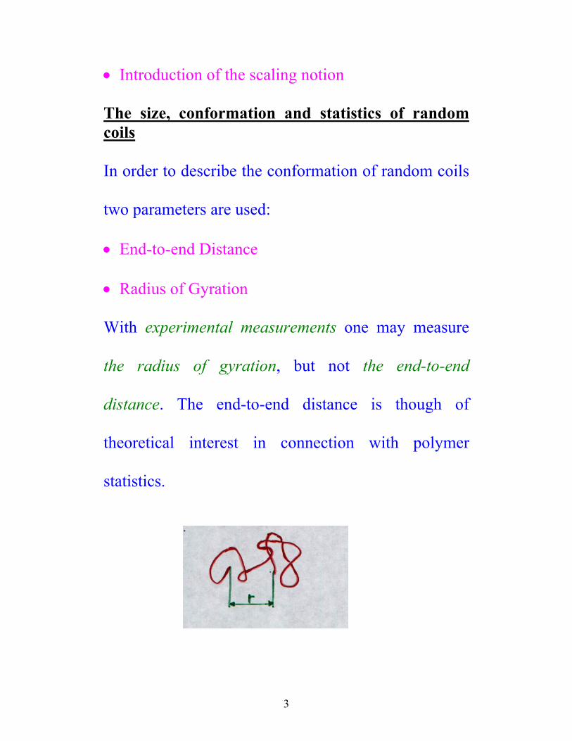
4
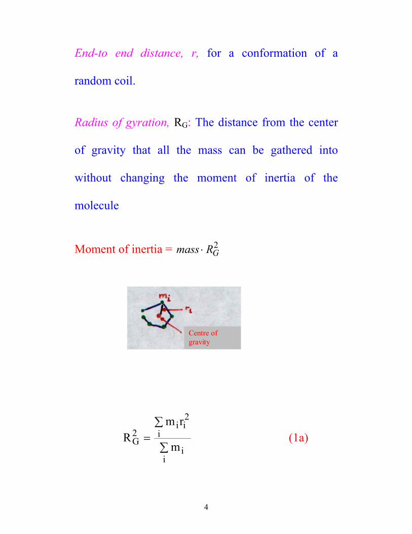
End-to end distance, r, for a conformation of a
random coil.
Radius of gyration, RG: The distance from the center
of gravity that all the mass can be gathered into
without changing the moment of inertia of the
molecule
Moment of inertia = 2
GRmass ⋅
Rm r
mG
i ii
ii
2
2
=∑
∑ (1a)
Centre of gravity
5
Rm r
mG
i ii
ii
2
2
=∑
∑ (1b)
R Rm r
mG G
i ii
ii
= =∑
∑
( )/
/
2 1 22 1 2
(1c)
If all mass points have an identical mass, M0:
m r M ri i iii
20
2= ∑∑ and m n Mii
= ⋅∑ 0
(n = number of monomer units)
From equ. (1c):
Rr
nG
ii=∑
2 1 2/
(2a)
6
Rr
nG
ii=∑
21 2
1 2
/
/ (2b)
Rr
nG
ii2
2
=∑
(2c)
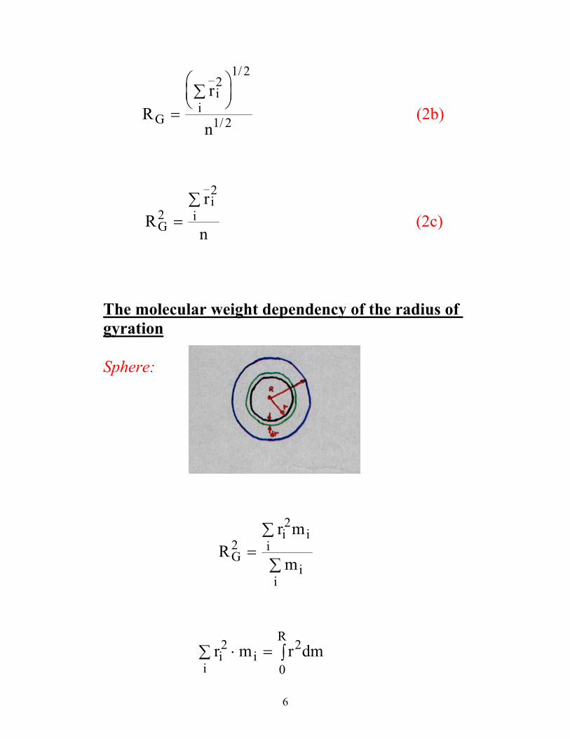
The molecular weight dependency of the radius of gyration Sphere:
Rr m
mG
i ii
ii
2
2
=∑
∑
r m r dmii
iR2 2
0∑ ⋅ = ∫
7
)Vm(drr4dm 2 =ρ⋅ρ⋅π⋅= ; (V=4πr2dr)
∫⋅ρ⋅π⋅
=⋅ρ⋅⋅π⋅=∑ ⋅R
0
54
ii
2i 5
R4drr4mr
⟩∫ ++
=⟨+
.1
)1(const
nxdxx
nn
3
R4drr4m3R
0
2
ii
⋅ρ⋅π⋅=⋅∫ ⋅ρ⋅π⋅=∑
3
5
2G
R34
R54
R⋅ρ⋅π⋅
⋅ρ⋅π⋅=
R R R RG G2
2 1 235
35
= = ⋅
;/
volumespesificpartialthevNMvvolumeV
A=⋅= ;)(
V R R v MNA
=⋅ ⋅
=⋅ ⋅⋅ ⋅
43
34
33π
π;
8
R vN
MGA
=
⋅⋅ ⋅
⋅
35
34
1 2 1 31 3
/ //
π
3/1. MconstRG ⋅= (3)
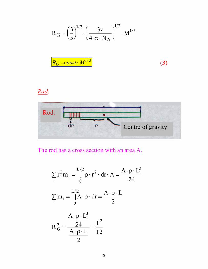
Rod:
Rod:
Centre of gravity
The rod has a cross section with an area A.
24
LAAdrrmr32/L
0
2
ii
2i
⋅ρ⋅=∫ ⋅⋅⋅ρ=∑
2
LAdrAm2/L
0ii
⋅ρ⋅=∫ ⋅ρ⋅=∑
12L
2LA
24LA
R2
3
2G =
⋅ρ⋅
⋅ρ⋅
=
9
LconstRG ⋅= .
MconstRG ⋅= . (4)
Random coil
Thermodynamic good conditions:
RG ∝ M0.60 (”Mean-field” approximation)
Rg ∝ M0.588 (”Renormalization group theory”)
θ-Conditions: Rg ∝ M0.50
The relation between RG and the end-to-end
distance, ri, in the molecule
10
For linear flexible polymers the following relation
between chain distance (r) and the radius of gyration
is valid:
( ) ( )R r r RG G2
22 1 2 2 1 2
66= =;
/ / (5)
(---)1/2 Root-mean-square (r.m.s.)-average.
( )r n r n r n rn n n
i i
i
2 1 21 1
22 2
2 2
1 2
1 2/ /
=+ + •••+ + ••
Models for random coils
1) Chain molecules with a kind of given, locked,
rigid structure.
11
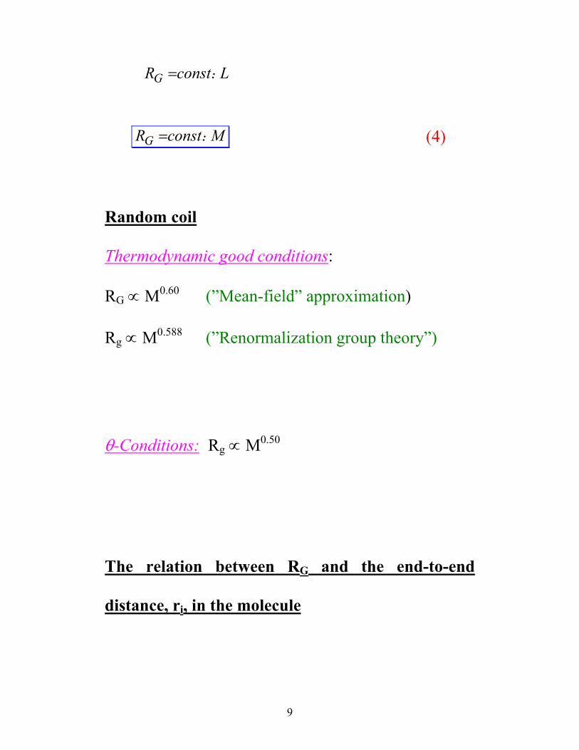
a) Totally extended chain:
LK = l·n
n = number of bonds; l = bond length; LK = contour length
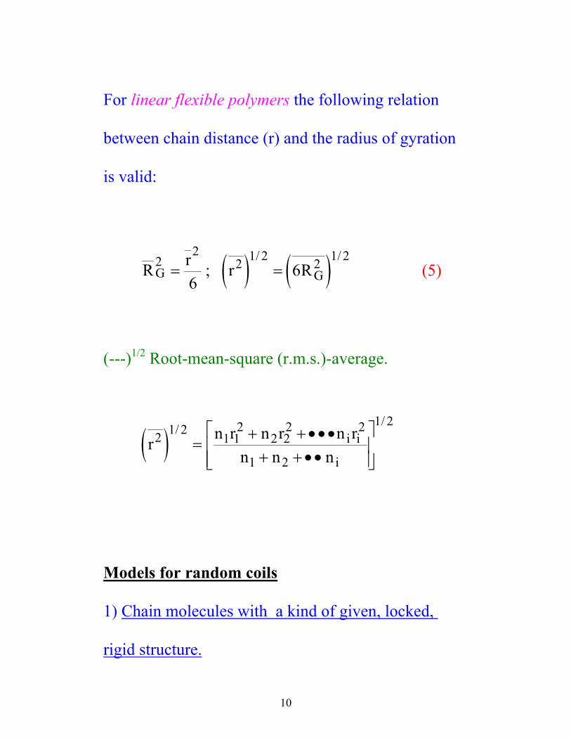
b) Chain with a zigzag structure
r n l= ⋅ ⋅sin( )θ2
This chain has a locked bond angle that assures that
the chain may have only one conformation, and that it
is completely rigid.
12
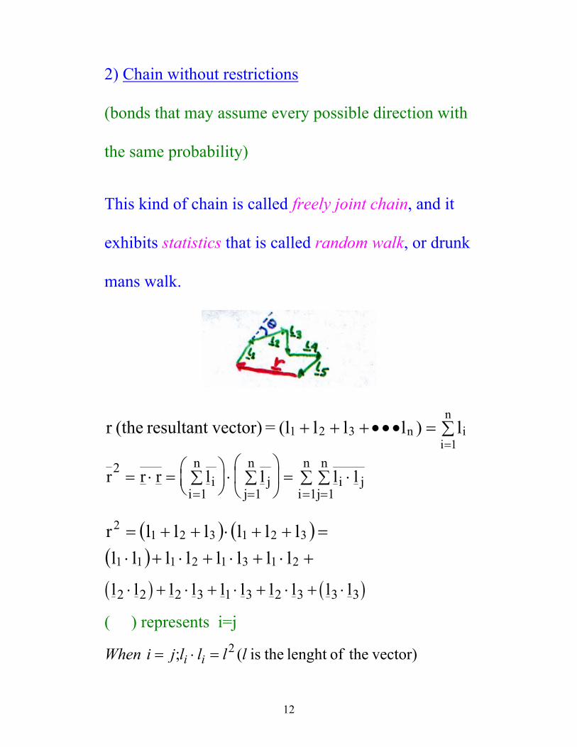
2) Chain without restrictions
(bonds that may assume every possible direction with
the same probability)
This kind of chain is called freely joint chain, and it
exhibits statistics that is called random walk, or drunk
mans walk.
∑=•••+++=
n
1iin321 l)llll( = vector)resultant (the r
r r r l l l lii
nj
j
ni j
j
n
i
n2
1 1 11= ⋅ = ∑
⋅ ∑
= ⋅∑∑
= = ==
( ) ( )( ) +⋅+⋅+⋅+⋅
=++⋅++=
21312111
3213212
llllllllllllllr
( ) ( )l l l l l l l l l l2 2 2 3 1 3 2 3 3 3⋅ + ⋅ + ⋅ + ⋅ + ⋅
( ) represents i=j
vector) theoflenght theis (; 2 lllljiWhen ii =⋅=
13
If we have n monomers in the chain, we have (n-1)≈n
vectors. We assume that all bonds is of the same
length l and multiply out all i=j, we get the square-
average of the end-to-end-distance
⟨ ⟩ = ⋅ + ⟨ ⋅ ⟩ ≠∑∑==
r n l l l i ji jj
n
i
n2 2
11( ) (6)
For li · lj with i ≠ j, we get:
vectors.ebetween th angle theis where;cos2 θθ ⟩⟨⋅=⟩⋅⟨ lll ji
For a random coil all values of θ are equally probable
⟨ ⟩ = ⟨ ⟩ = ⋅cos ;θ 0 2 2r n l
⟨ ⟩ = ⋅r n l1 2/ (7)
14
For a rod like particle the equivalent expression is:
r = n · l (8)
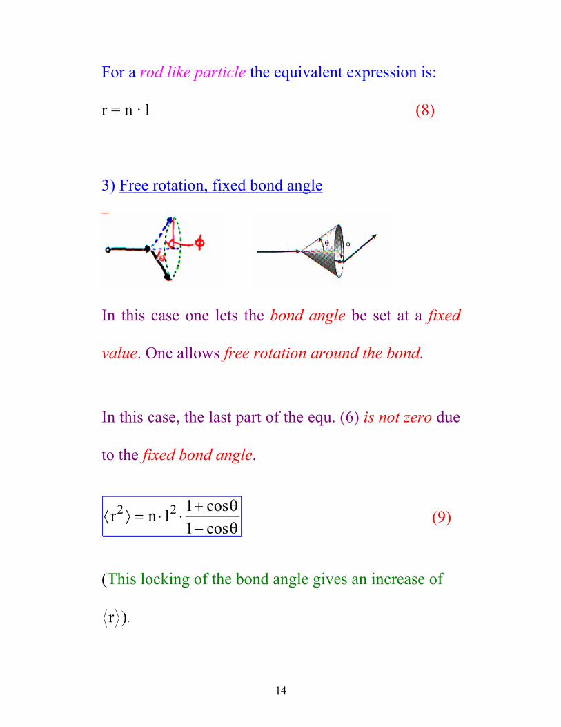
3) Free rotation, fixed bond angle
In this case one lets the bond angle be set at a fixed
value. One allows free rotation around the bond.
In this case, the last part of the equ. (6) is not zero due
to the fixed bond angle.
⟨ ⟩ = ⋅ ⋅+−
r n l2 2 11
coscos
θθ
(9)
(This locking of the bond angle gives an increase of
r ).
15
Equ. (8) and (9) is only valid when the end-to-end
distance exhibits a Gauss distribution.
If we identify this bond angle with the tetraeder-angle
(θ = 109o) we get equ. (9):
22 ln00.2r ⋅⋅=⟩⟨ (10)
If we compare this result with the experimental result
for polyethylene:
22 ln)3.07.6(r ⋅⋅±=⟩⟨
we observe that this model gives too small values.
16
4) Hindered rotation
We will now take into consideration a fact that is
often the case for polymer chains, namely when the
rotation around the single bonds is not free.
For a complete description of the conformation of a
model chain, we have to have information of both the
bond angle (θ) and the rotation angle (φ) (torsion
angle).
⟨ ⟩ = ⋅ ⋅ +−
⋅ + ⟨ ⟩− ⟨ ⟩
r n l2 2 11
11
coscos
coscos
θθ
φφ
(11)
rotation)(hindered0cos;rotation) (free 0cos ≠⟩⟨=⟩⟨ φφ
17
Equ. (11) takes into account trans- and gauche-
conformations. If the gauche- and trans-
conformations have the same energy: cosφ = 0
Real polymer chains (short-range interactions)
The end-to-end distance, r, for a polymer chain with a
fixed bound angle, θ, and the rotation angle, φ, may
be written as:
⟨ ⟩ = ⋅ ⋅+−
⋅+ ⟨ ⟩− ⟨ ⟩
r n l2 2 11
11
coscos
coscos
θθ
φφ
Let us now replace the real bound length l with a
fictive bound length, β, which is called the effective
bound length:
⟨ ⟩ = ⋅r n2 2β
18
The ratio β1
is a measure of the stiffness of the
polymer chain.
Cl
=β2
2 : the characteristic ratio.
Ex.: Polymer C Polyethylene 6.8 Polystyrene 9.9 Polyethylene oxide 4.1 Polybuthadiene 4.8
Definition of the Kuhn length lku
We may generally describe a statistic chain molecule
with the aid of the concept equivalent statistic
segment. In this case we imagine that instead of
contemplating a chain that consists of real segments
with a hindered rotation around the bonds and fixed
bond angles, we make a hypothetical statistic chain
19
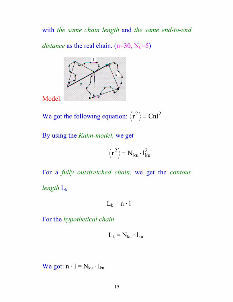
with the same chain length and the same end-to-end
distance as the real chain. (n=30, Nk =5)
Model:
We got the following equation: r Cnl2 2=
By using the Kuhn-model, we get
r N lku ku2 2= ⋅
For a fully outstretched chain, we get the contour
length Lk
Lk = n · l
For the hypothetical chain
Lk = Nku · lku
We got: n · l = Nku · lku
20
l n l N l C n lku ku ku⋅ ⋅ = ⋅ = ⋅ ⋅2 2
l C lku = ⋅
N nCku =
We see from these two equations that the stiffer the
molecule, the longer is the Kuhn-segment, while there
will be a smaller number of Kuhn-segments.
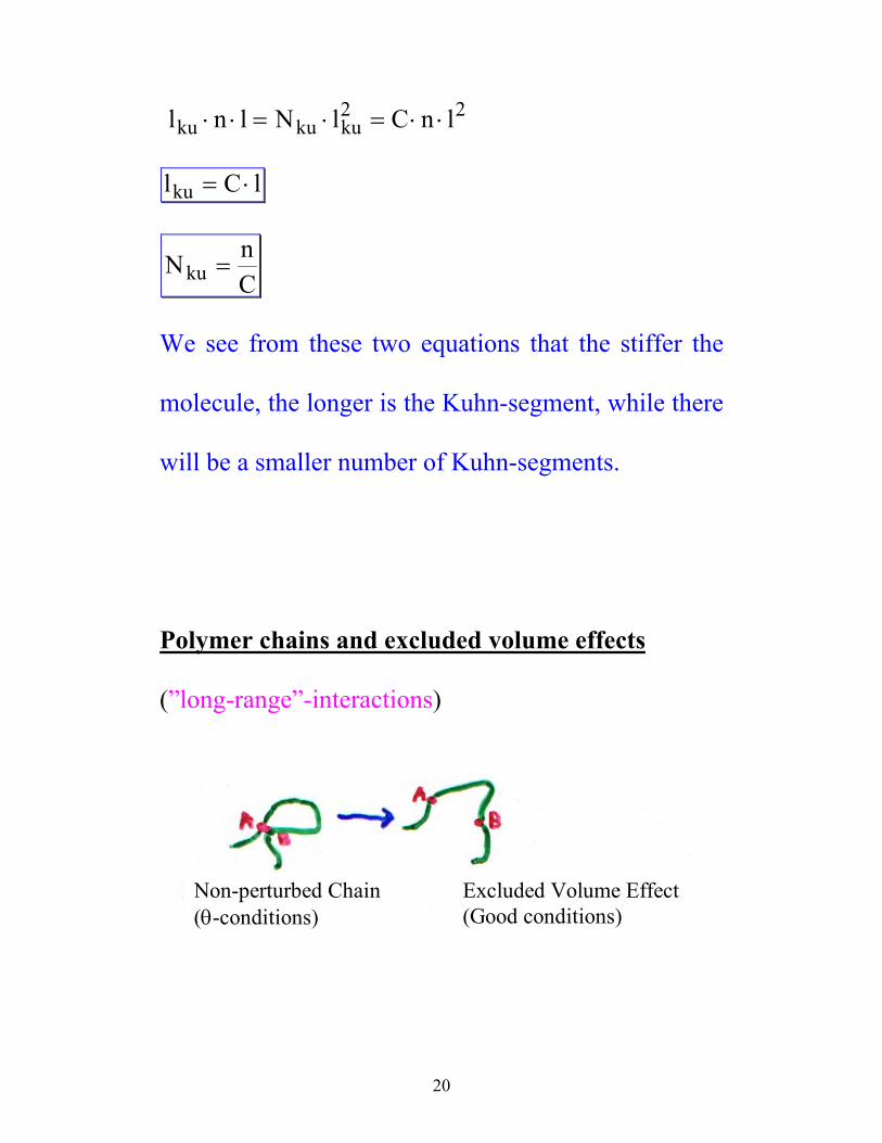
Polymer chains and excluded volume effects (”long-range”-interactions)
Non-perturbed Chain (θ-conditions)
Excluded Volume Effect (Good conditions)
21
r n
r
r
2 2 2
2 1 2
20
1 2
= ⋅ ⋅
=
α β
α
/
/
α = expansion coefficient.
r20
1 2/ = the ideal conformation or the non-perturbed
dimension.
Polymer molecules have the dimension r20
1 2/ in a θ-
solvent (ideal solvent).
Thermodynamic good solvents: α > 1
θ-solvents: α = 1
Thermodynamic poor solvents: α < 1
22
Interactions and size of chain molecules at different
thermodynamic conditions.
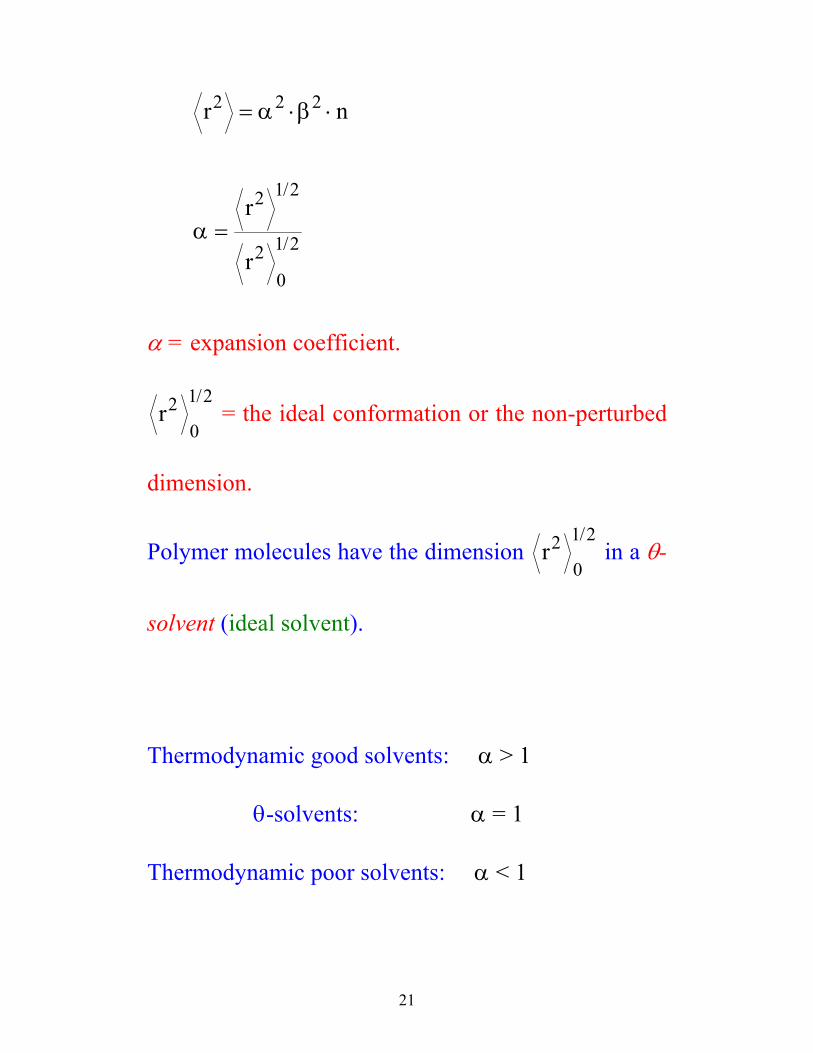
Potential curve
Lennard-Jones
potential:V r V rr
rre( ) =
−
− −
40
12
0
6
1. At short distances repulsion between the
monomers
2. At long distances attractive interactions between
the monomers
23
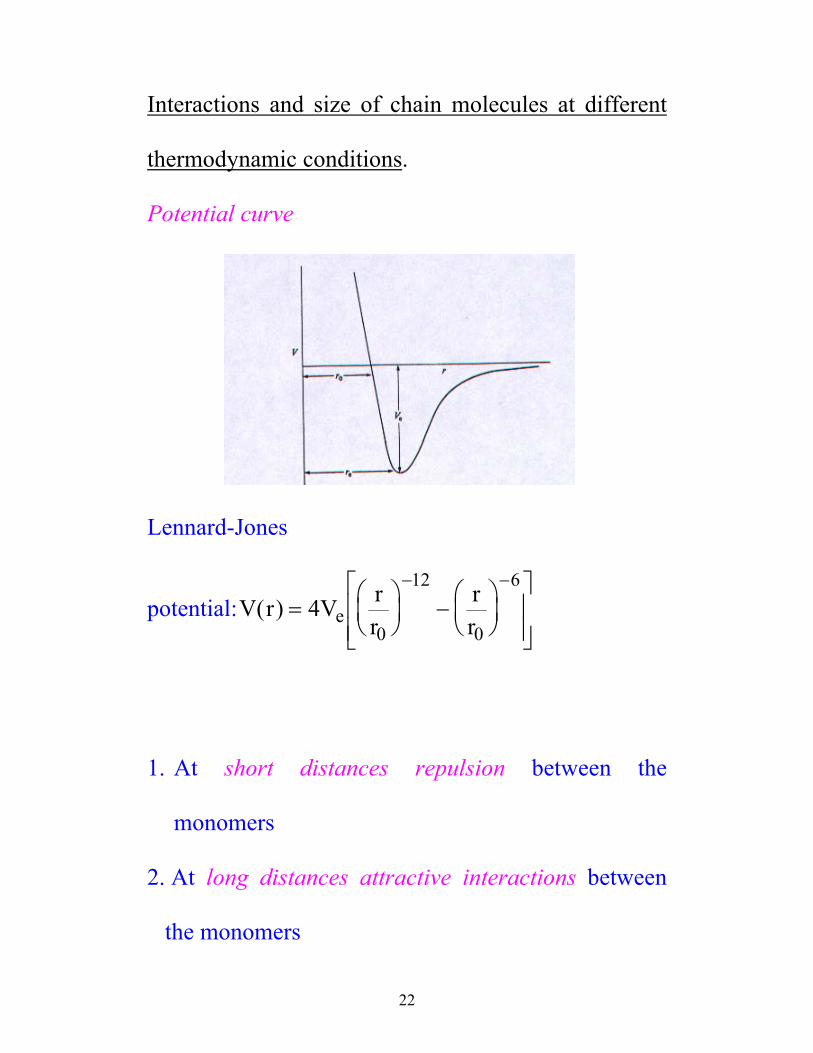
Poor conditions θ-conditions Good conditions
R MG ∝ 1 3/ R MG ∝ 1 2/ 6.0G MR ∝
”Globule” attractive mon.-mon. interactions. α < 1; v < 0 v is the excluded volume parameter
The attractive and repulsive interactions compensate each other. Ideal chain α = 1; v = 0 Gaussian statistics
Repulsive interactions leads to an expansion of the chain. α > 1; v > 0 Excluded volume statistics
24
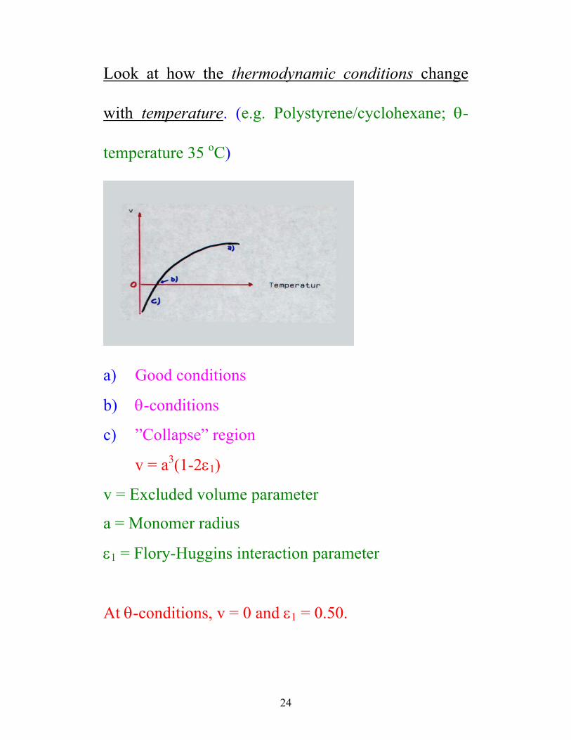
Look at how the thermodynamic conditions change
with temperature. (e.g. Polystyrene/cyclohexane; θ-
temperature 35 oC)
a) Good conditions
b) θ-conditions
c) ”Collapse” region
v = a3(1-2ε1)
v = Excluded volume parameter
a = Monomer radius
ε1 = Flory-Huggins interaction parameter
At θ-conditions, v = 0 and ε1 = 0.50.
25
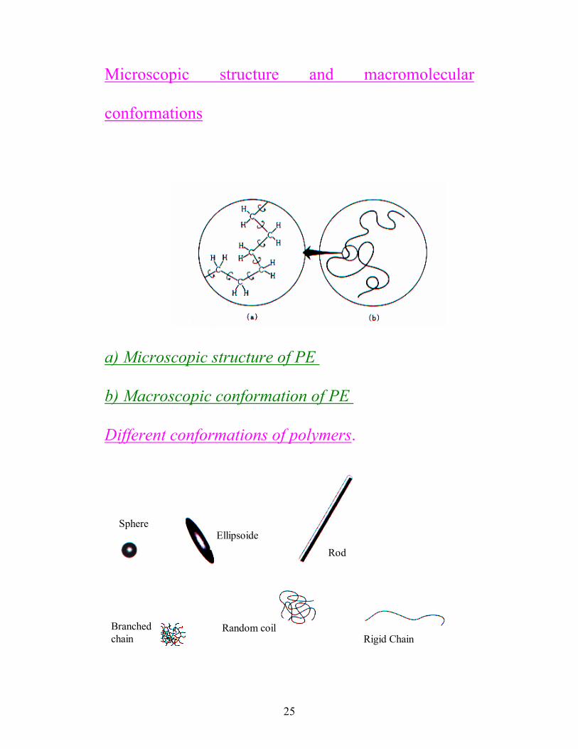
Microscopic structure and macromolecular
conformations
a) Microscopic structure of PE
b) Macroscopic conformation of PE
Different conformations of polymers.
Sphere
Ellipsoide
Rod
Branched chain
Random coil
Rigid Chain
26
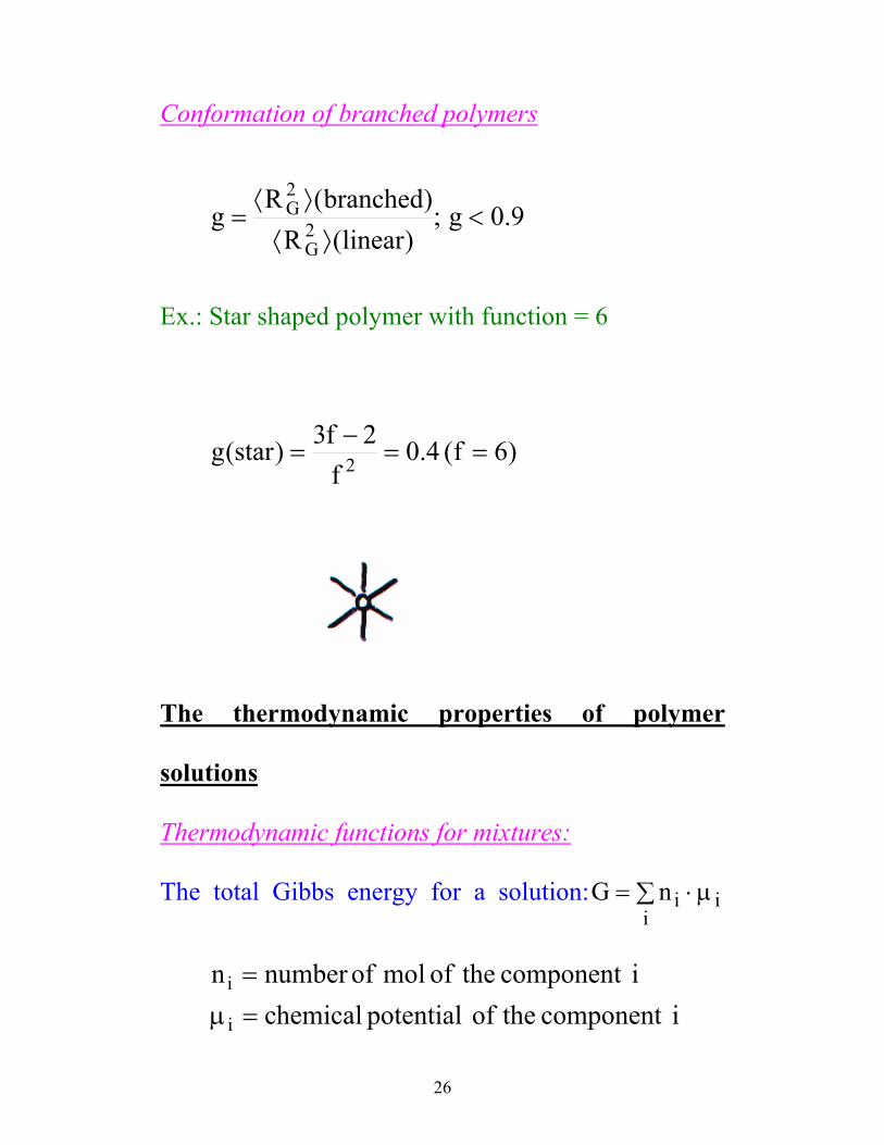
Conformation of branched polymers
9.0g;)linear(R
)branched(Rg 2G
2G <
⟩⟨⟩⟨
=
Ex.: Star shaped polymer with function = 6
)6f(4.0f
2f3)star(g 2 ==−
=
The thermodynamic properties of polymer
solutions
Thermodynamic functions for mixtures:
The total Gibbs energy for a solution:G ni ii
= ⋅∑ µ
icomponent theof potential hemicalc
icomponent theof mol ofumbernn
i
i
=µ=
27
Change in Gibbs molar energy for a mixture:
( )∆G n G nm i i ii
i ii
= −∑ = − ∑µ µ µ0 0
µ i0 = chemical potential in the standard condition
(pure substance).
In the same way the change in mixing enthalpy is
defined:
( )∆H n H H H n Hm i i ii
i i= −∑ = − ∑0 0
and mixing entropy:
( )∆
∆ ∆ ∆
S n S S S n S
G H T S
m i i ii
i ii
m m m
= −∑ = − ∑
= −
0 0
(Gibbs - Helmholz)
28
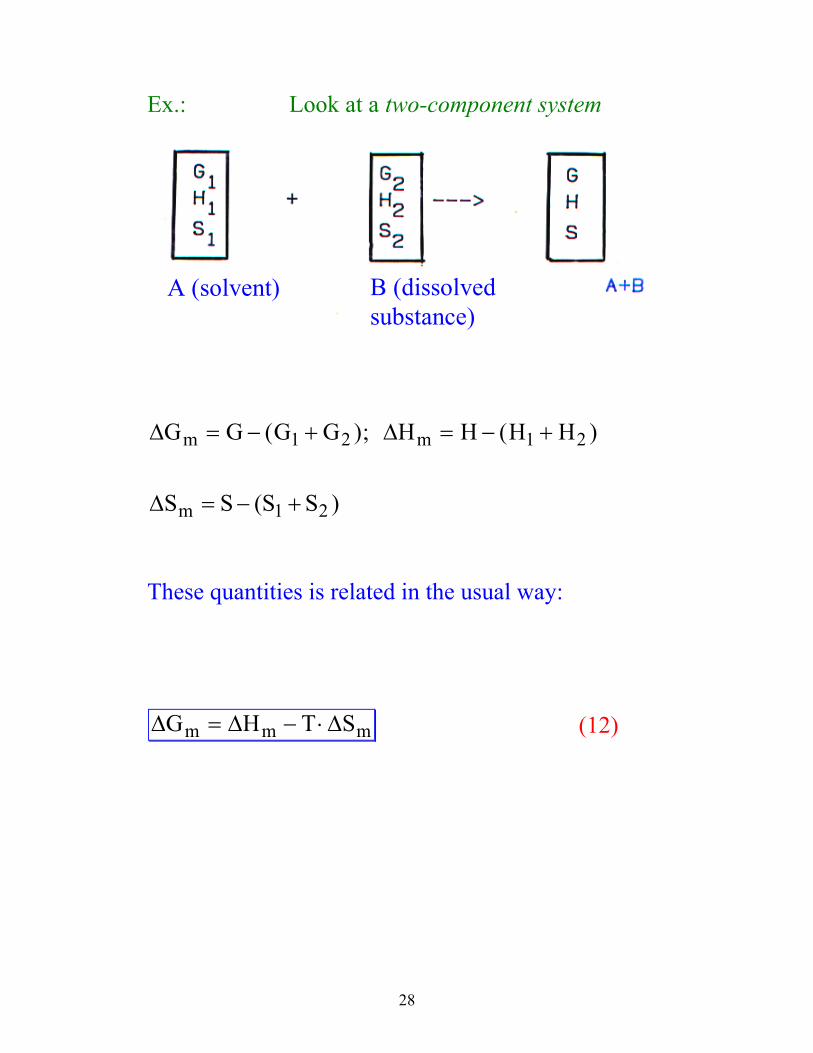
Ex.: Look at a two-component system
A (solvent) B (dissolved substance)
∆ ∆
∆
G G G G H H H H
S S S
m m
m
= − + = − +
= − +
( ); ( )
(S )
1 2 1 2
1 2
These quantities is related in the usual way:
∆ ∆ ∆G H T Sm m m= − ⋅ (12)
29
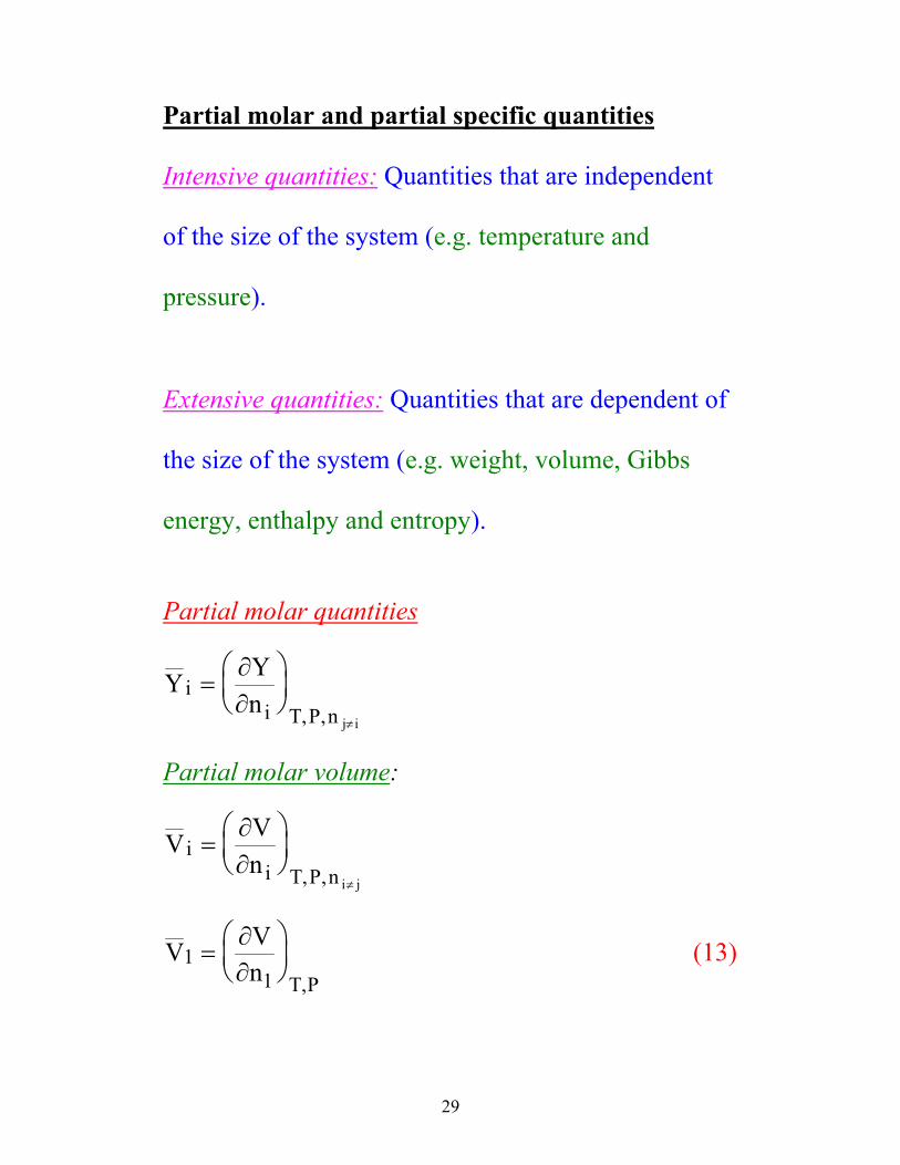
Partial molar and partial specific quantities
Intensive quantities: Quantities that are independent
of the size of the system (e.g. temperature and
pressure).
Extensive quantities: Quantities that are dependent of
the size of the system (e.g. weight, volume, Gibbs
energy, enthalpy and entropy).
Partial molar quantities
Y Yn
ii T P n j i
=
≠
∂∂ , ,
Partial molar volume:
V Vn
ii T P n i j
=
≠
∂∂ , ,
V Vn T P
11
=
∂∂ ,
(13)
30
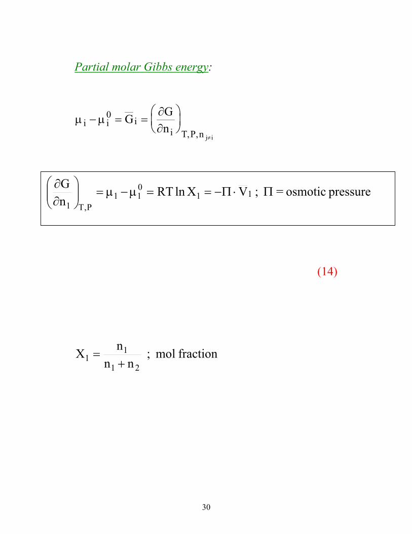
Partial molar Gibbs energy:
µ µ∂∂i i i
i T P nG G
nj i
− = =
≠
0
, ,
(14)
fractionmol ; nn
nX21
11 +=
pressure osmotic = ; VXlnRTnG
11011
P,T1Π⋅Π−==µ−µ=
∂∂
31
Partial specific quantities:
y Ygi
i T P g j i
=
≠
∂∂ , ,
gi is the weight of component i. Partial specific volume:
v Vg
ii T P g j i
=
≠
∂∂ , ,
The relation between partial molar and partial specific
quantities is:
i
ii
MVv = ; where Mi is the molecular weight of
component i
32
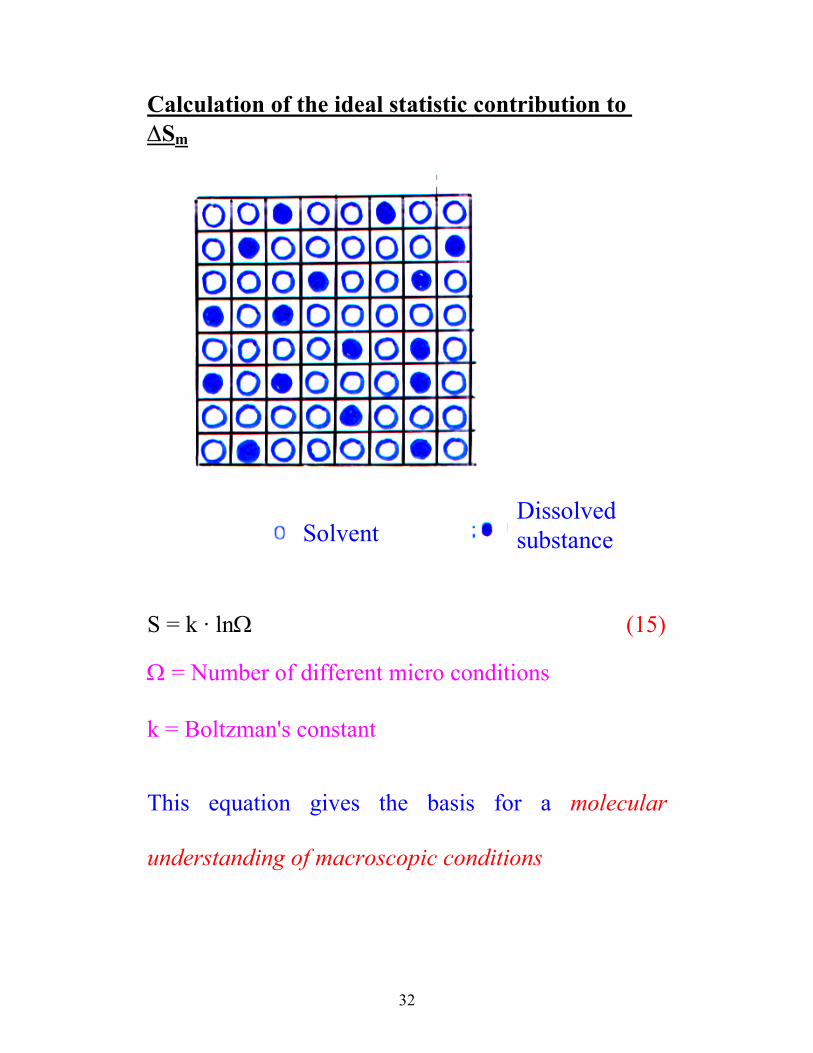
Calculation of the ideal statistic contribution to ∆Sm
SolventDissolved substance
S = k · lnΩ (15)
Ω = Number of different micro conditions
k = Boltzman's constant
This equation gives the basis for a molecular
understanding of macroscopic conditions
33
Statistical considerations of a two/component system
N0 = N1 + N2
N0 = total number of lattice positions N1 = number of solvent molecules N2 = number of molecules of the dissolved substance
There are N0 ways to arrange the first molecule, and
N0-1 ways to arrange the second molecule in the
lattice. There are N0(N0-1) ways to arrange the two
first molecules etc.
Ω' ( ) ( ) ( ) != − ⋅ − ⋅ − ⋅⋅⋅ =N N N N N0 0 0 0 01 2 3
We have to correct Ω’ with the number of ways N1
and N2 molecules may be permutated
34
Ω =⋅
NN N
0
1 2
!! !
(16)
For the pure components:
Ω Ω1 21
1
2
21= = = =
NN
NN
!!
!!
35
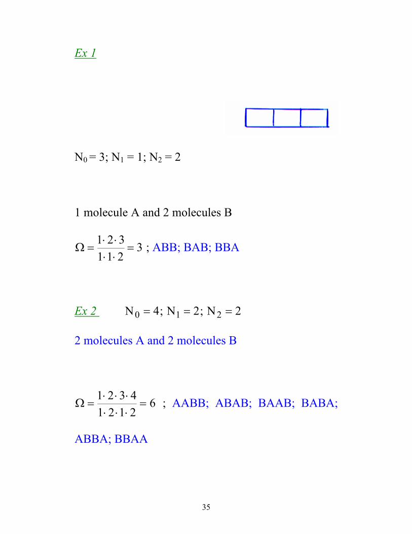
Ex 1
N0 = 3; N1 = 1; N2 = 2
1 molecule A and 2 molecules B
Ω =⋅ ⋅⋅ ⋅
=1 2 31 1 2
3 ; ABB; BAB; BBA
Ex 2 N N N0 1 24 2 2= = =; ;
2 molecules A and 2 molecules B
Ω =⋅ ⋅ ⋅⋅ ⋅ ⋅
=1 2 3 41 2 1 2
6 ; AABB; ABAB; BAAB; BABA;
ABBA; BBAA
36
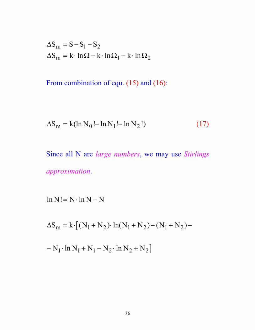
∆∆ Ω Ω Ω
S S S SS k k k
m
m
= − −= ⋅ − ⋅ − ⋅
1 2
1 2ln ln ln
From combination of equ. (15) and (16):
∆S k N N Nm = − −(ln ! ln ! ln !)0 1 2 (17)
Since all N are large numbers, we may use Stirlings
approximation.
ln ! lnN N N N= ⋅ −
[
]
∆S k N N N N N N
N N N N N N
m = ⋅ + ⋅ + − + −
− ⋅ + − ⋅ +
( ) ln( ) ( )
ln ln
1 2 1 2 1 2
1 1 1 2 2 2
37
[
]
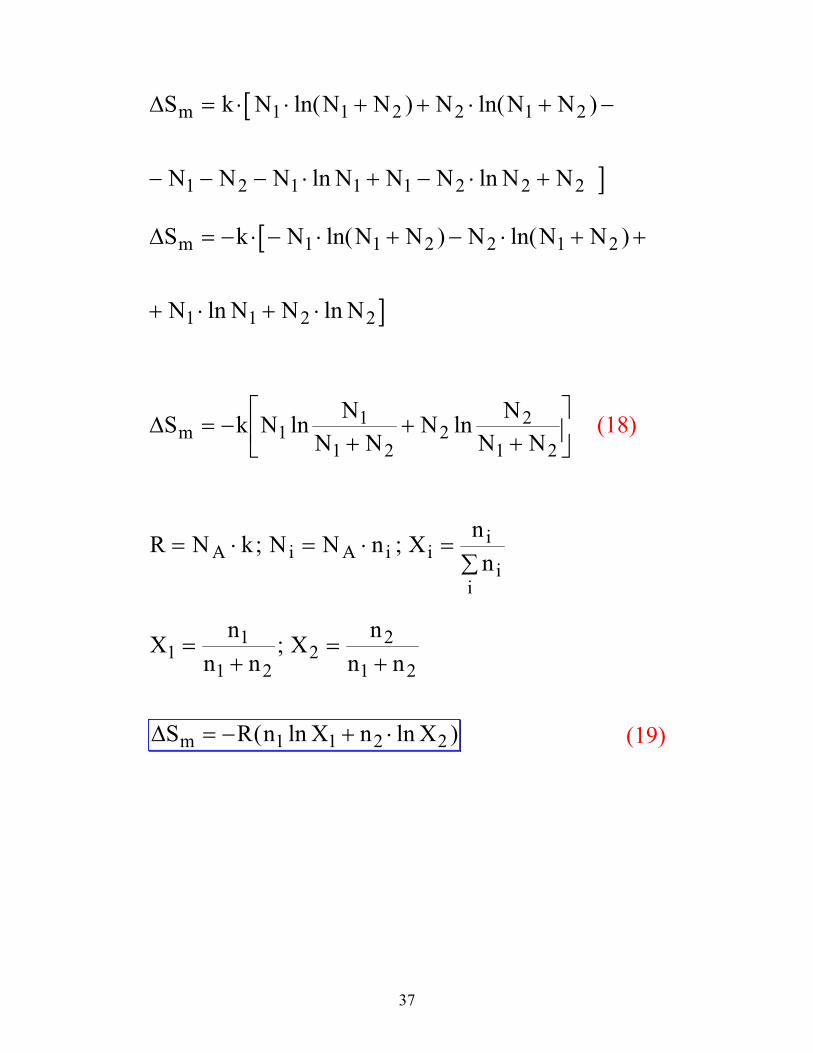
∆S k N N N N N N
N N N N N N N N
m = ⋅ ⋅ + + ⋅ + −
− − − ⋅ + − ⋅ +
1 1 2 2 1 2
1 2 1 1 1 2 2 2
ln( ) ln( )
ln ln
[
]
∆S k N N N N N N
N N N N
m = − ⋅ − ⋅ + − ⋅ + +
+ ⋅ + ⋅
1 1 2 2 1 2
1 1 2 2
ln( ) ln( )
ln ln
∆S k N NN N
N NN Nm = −
++
+
1
1
1 22
2
1 2ln ln (18)
R N k N N n X nnA i A i ii
ii
= ⋅ = ⋅ =∑
; ;
X nn n
X nn n1
1
1 22
2
1 2=
+=
+;
∆S R n X n Xm = − + ⋅( ln ln )1 1 2 2 (19)
38
If we assume that the solution is ideal, then ∆Hm = 0.
From equ. (12):
∆G R T n X n Xm = ⋅ ⋅ ⋅ + ⋅( ln ln )1 1 2 2 (20)
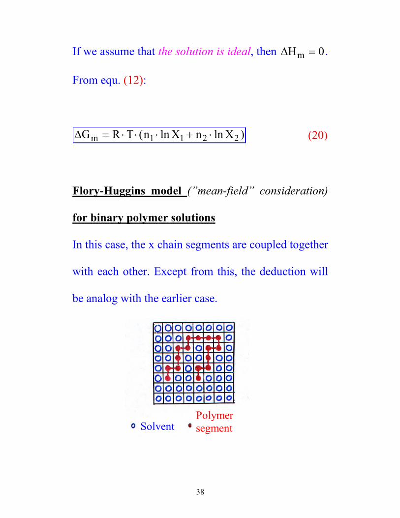
Flory-Huggins model (”mean-field” consideration)
for binary polymer solutions
In this case, the x chain segments are coupled together
with each other. Except from this, the deduction will
be analog with the earlier case.
SolventPolymer segment
39
N N x N0 1 2= + ⋅
∆S k N NN x N
N xNN x Nm = − ⋅
+ ⋅+ ⋅
+ ⋅
1
1
1 22
2
1 2ln ln (21)
Compare with equ. (18).
The volume fraction for the solvent ( )Φ1 and for the
polymer ( ).Φ2
21
22
21
11 NxN
Nx;NxN
N⋅+
⋅=Φ
⋅+=Φ
( )∆ Φ ΦS R n nm = − ⋅ + ⋅1 1 2 2ln ln (22)
It is important to point out equ. (22) only represent the
configuration entropy of the mixture.
40
In addition there may exist an other type of entropy
that is due to specific interactions between polymer-
and solvent molecules.
In Flory-Huggins theory we assume that ∂H ≠ 0
because the polymer-solvent interaction energies are
different from the polymer-polymer and solvent-
solvent interaction energies.
Mixing enthalpy for polymer and solvent Type of contacts Interaction energies
Solvent-solvent (1,1) w11
Polymer-polymer (2,2) w22
Solvent-polymer (1,2) w12
41
The dissolving process may be written as the change
of these contacts:
( , ) / ( , ) / ( , )11 1 2 2 2 1 2 1 2⋅ + ⋅ → The difference in energy, ∆w, is: ∆w w w w= − + ⋅12 11 22 1 2( ) / If the average number of 1,2 contacts in the solution is
P1,2 (over all lattice configurations), the mixing
enthalpy is:
∆ ∆
Φ
∆ Φ ∆
H w PP x N Z
H x N Z w
m
m
= ⋅
= ⋅ ⋅ ⋅
= ⋅ ⋅ ⋅ ⋅
1 2
1 2 2 1
2 1
,
,
Φ1 = the probability of 1,2 contacts
Z = the coordination number for a certain lattice
position
42
From the definition of volume fraction, we get (by
dividing these with each other):
x N N H N Z wm⋅ ⋅ = ⋅ = ⋅ ⋅ ⋅2 1 1 2 1 2Φ Φ ∆ Φ ∆;
Let us now define a new parameter ε1 (Flory-Huggins
parameter) that expresses polymer-solvent
interactions:
Z w k T Z wk T
⋅ = ⋅ ⋅ =⋅⋅
∆∆
ε ε1 1;
∆ Φ ΦH N k T n R Tm = ⋅ ⋅ ⋅ = ⋅ ⋅ ⋅1 2 1 1 2 1ε ε (23)
43
We now got equations for ∆Sm (equ. 22) and ∆Hm:
( )∆ Φ Φ ΦG R T n n nm = ⋅ ⋅ ⋅ + +1 2 1 1 1 2 2ε ln ln (24) This equation transforms into equ. (20) when
x = 1 and ε1 = 0.
The use of Flory-Huggins theory to calculate the
partial molar Gibbs energy
∆∆G G
nm
T P1
1=
∂∂
( )
, ; diff.equ. (24)
∂Φ∂
⋅⋅ε+Φ⋅ε+Φ⋅
∂Φ∂
+Φ+Φ⋅
∂Φ∂
⋅=∆222 n1
21121
2
2
n1
21
1
1
n1
11
nnn
nlnn
nRTG
(25)
44
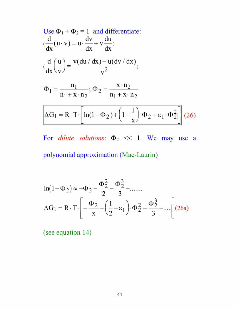
Use Φ1 + Φ2 = 1 and differentiate:
(ddx
u v u dvdx
v dudx
( )⋅ = ⋅ + )
(ddx
uv
v du dx u dv dxv
=
−( / ) ( / )2 )
Φ Φ11
1 22
2
1 2=
+ ⋅=
⋅+ ⋅
nn x n
x nn x n
;
∆ Φ Φ ΦG R Tx
1 2 2 1 221 1 1
= ⋅ ⋅ − + −
⋅ + ⋅
ln( ) ε (26)
For dilute solutions: Φ2 << 1. We may use a
polynomial approximation (Mac-Laurin)
( )ln .......12 32 222
23
− ≈ − − − −Φ ΦΦ Φ
∆Φ
ΦΦG R T
x1 2
1 22 2
312 3
= ⋅ ⋅ − − −
⋅ − −
ε ..... (26a)
(see equation 14)
45
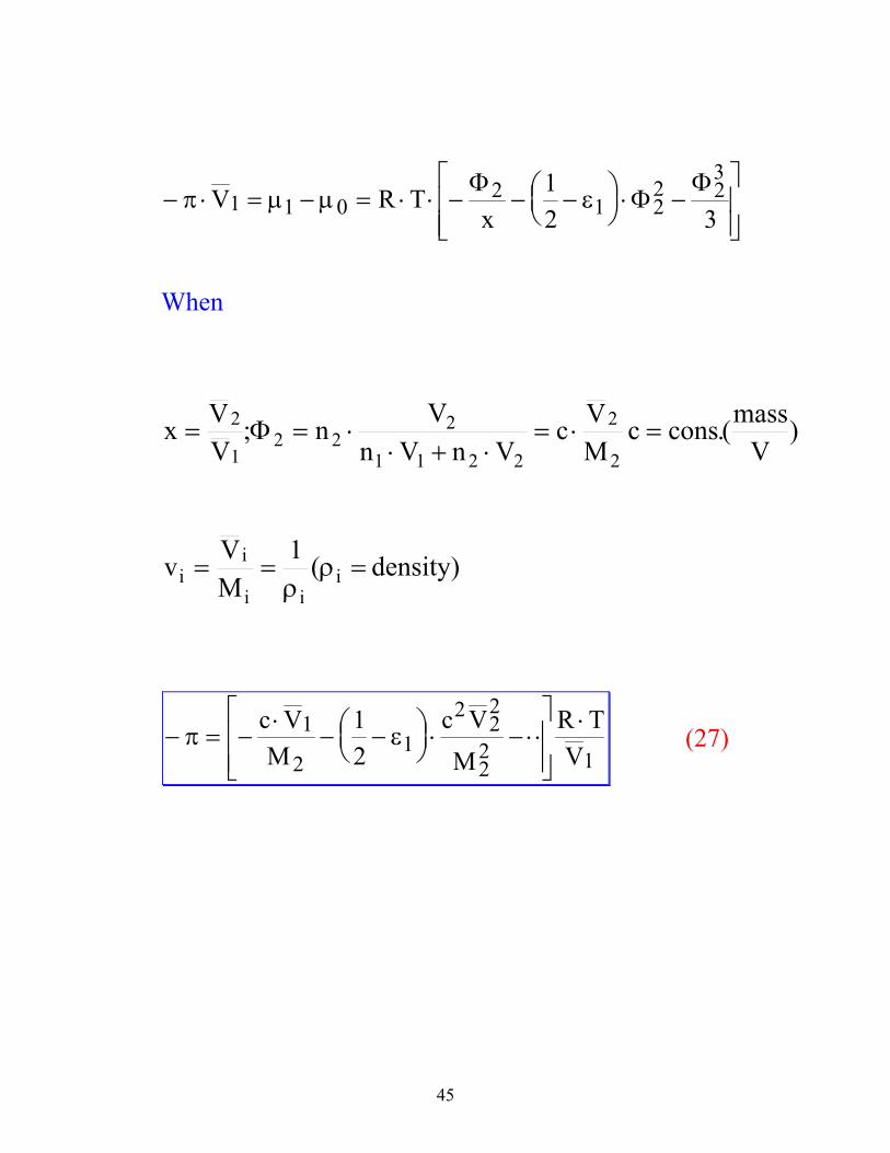
− ⋅ = − = ⋅ ⋅ − − −
⋅ −
π µ µ εV R Tx
1 1 02
1 22 2
312 3
ΦΦ
Φ
When
)V
mass(.conscMVc
VnVnVn;
VVx
2
2
2211
222
1
2 =⋅=⋅+⋅
⋅=Φ=
density) (1MVv i
ii
ii =ρ
ρ==
− = −⋅
− −
⋅ − ⋅⋅
⋅π ε
c VM
c VM
R TV
1
21
222
22 1
12
(27)
46
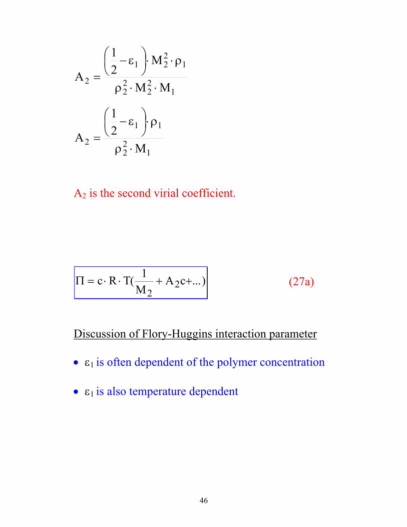
122
22
1221
2 MM
M21
A⋅⋅ρ
ρ⋅⋅
ε−
=
122
11
2 M21
A⋅ρ
ρ⋅
ε−
=
A2 is the second virial coefficient.
Π = ⋅ ⋅ + +c R TM
A c( ...)12
2 (27a)
Discussion of Flory-Huggins interaction parameter
• ε1 is often dependent of the polymer concentration
• ε1 is also temperature dependent
47
• The experimental value of ε1 often diverges from
the theoretical value. This is related to the fact that
the Flory-Huggins parameter, ε1, consists of both
an enthalpy part and an entropy part.
ε = εH + εS; εS is constant
and
ε∂ε∂H TT
= − ⋅ ; the enthalpy is dependent of T
48
Flory-Krigbaum theory of dilute polymer solutions
Dilute Solution
The factor 12 1− ε may be viewed as a measure of the
deviation from the properties of an ideal solution.
This contribution to Gibbs molar energy is called
∆GE1 , and may consist of both enthalpy- and entropy
components:
∆ ΦG R TE1 1 1 2
2= ⋅ ⋅ − ⋅( )ψ τ (28) E = ”excess” τ1 = enthalpy parameter ψ1 = entropy parameter
E1
E1
E1 STHG ∆⋅+∆−=∆− (29)
49
∆ ΦH R TE1 1 2
2= ⋅ ⋅ ⋅τ (30)
∆ ΦS RE1 1 2
2= ⋅ ⋅ψ (31)
( )ψ τ ε1 1 112
− = −
∆ ∆ ∆G S HE E E1 1 10= → ⋅ =θ
θ ψ τ⋅ ⋅ ⋅ = ⋅ ⋅ ⋅R R T1 22
1 22Φ Φ
θτ
ψ=
⋅T 1
1
ψ τ ψθ
ε1 1 1 11 12
− = ⋅ −
= −
T (32)
One may express the expansion factor α in terms of
the Flory-temperature θ
α α ψθ5 3
11 22 1− = ⋅ ⋅ ⋅ −
⋅C
TMm
/ (33)
Cm is a constant.
50
We see that at the θ-temperature (T=θ), α=1. For high
molecular weights, equ 33 gives α5 ∝ M1/2 ⇒
α ∝ M0.1 6.0G5.0
G
,G
G M)good(R;MR
RR
∝∝=αθ
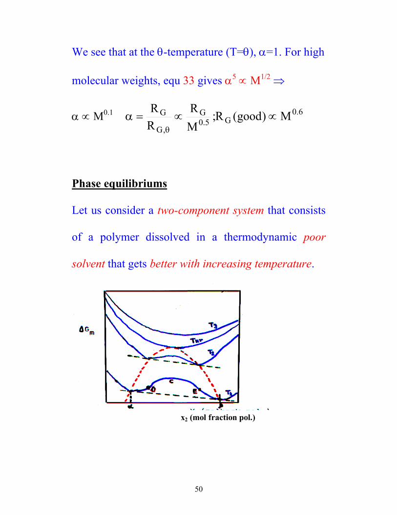
Phase equilibriums
Let us consider a two-component system that consists
of a polymer dissolved in a thermodynamic poor
solvent that gets better with increasing temperature.
x2 (mol fraction pol.)
51
Two phases α and β shares a common tangent. A
homogenous phase is stabile if X2 < α or X2 > β.
Thermodynamically unstable in the area α β≤ ≤X2 .
At T3 one has a system that is completely mixable.
Tkr = critical temperature for solubility.
D and E represents inflection points on the curve.
The striped red curve (the turbidity curve) represents
the heterogeneous two-phase region.
52
For the inflection points D and E the following
mathematical relation is valid:
0)G(and0)G(32
m3
22
m2
=Φ∂∆∂
=Φ∂∆∂
because D and E converge in the critical point. We
have used volume fraction, but the same is valid if
one uses mol fraction X.
0and0;)G(G 22
12
2
1i
i
mi =
Φ∂µ∂
=Φ∂∂µ
µ=Φ∂∆∂
=∆
We got: (see equ. 26)
µ µε1 0
2 2 1 221 1 1−
= − + − ⋅ +RT x
ln( ) ( )Φ Φ Φ
∂µ∂Φ
ε
∂ µ
∂Φε
1
2 21 2
21
22
22 1
11
1 1 2 0
1 11
2 0
= −−
+ − + ⋅ =
=− ⋅ −
−− ⋅ =
ΦΦ
Φ
,, ,
,,
( )
( ) ( )( )
cc c
cc
x
53
We may write the equations above in the following
way:
11
1 1 2 0
11
2 0
21 2
22 1
−− − − ⋅ =
−− ⋅ =
ΦΦ
Φ
,, ,
,,
( ) ( )
( )( )
cc c
cc
xa
b
ε
ε
By combining equation (a) and (b), we can derive the
following relations:
Φ2 1 21
1, /c
x=
+
ε1 1 2
2
1 212
1 1 12
12
1, / /c
x x x= ⋅ +
= + +
When 21and
x1;x c,12/1c,2 =ε=Φ∞→
54
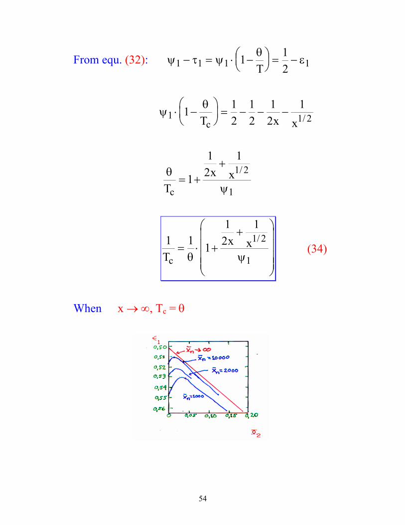
From equ. (32): ψ τ ψθ
ε1 1 1 11 12
− = ⋅ −
= −
T
ψθ
1 1 21 12
12
12
1⋅ −
= − − −
T x xc /
θ
ψTx x
c= +
+1
12
11 2
1
/
1 1 1
12
11 2
1Tx x
c= ⋅ +
+
θ ψ
/ (34)
When x → ∞, Tc = θ
55
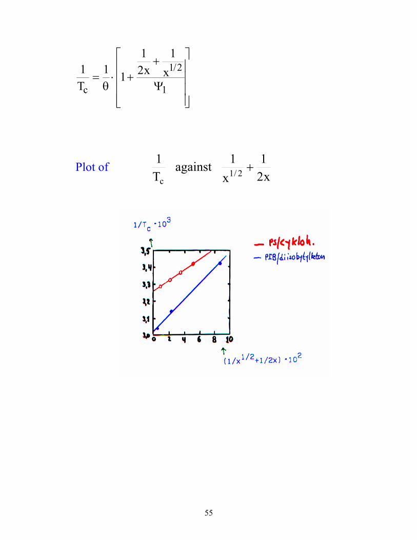
1 1 1
12
11 2
1Tx x
c= ⋅ +
+
θ
/
Ψ
Plot of x2
1x
1 against T1
2/1c
+
56
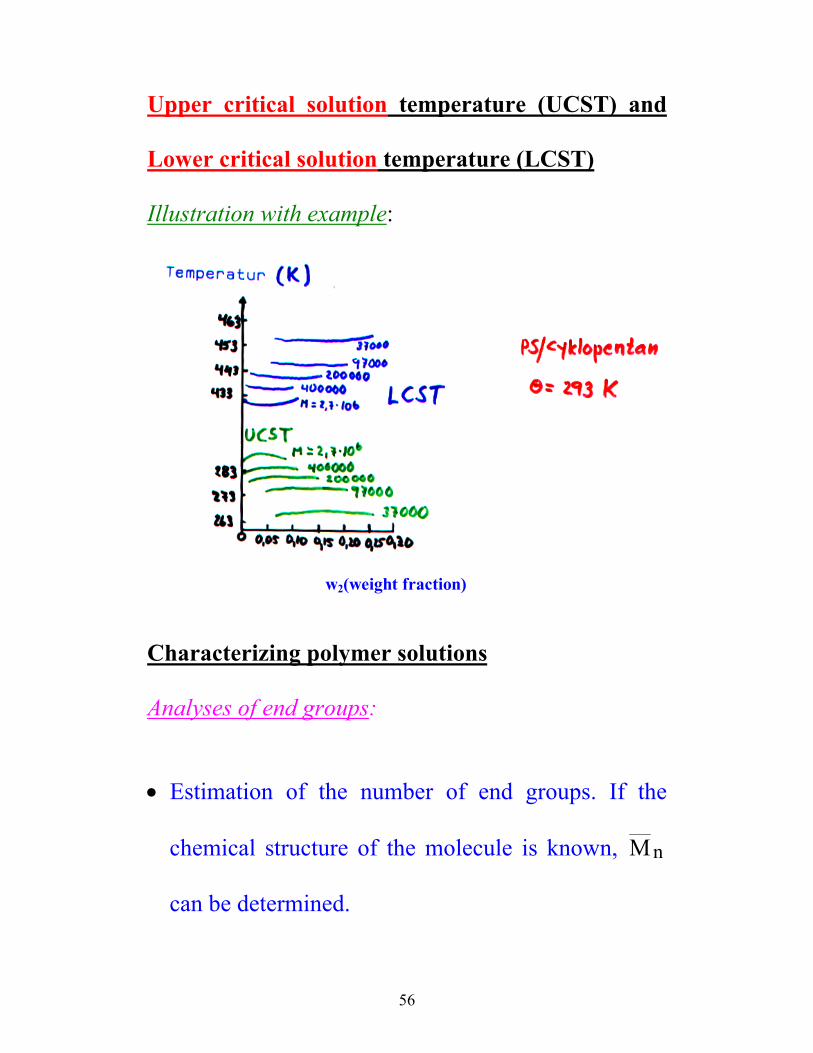
Upper critical solution temperature (UCST) and
Lower critical solution temperature (LCST)
Illustration with example:
w2(weight fraction)
Characterizing polymer solutions
Analyses of end groups:
• Estimation of the number of end groups. If the
chemical structure of the molecule is known, Mn
can be determined.
57
Methods that are used for analyses:
a) Chemical: Titration methods is often used
(carboxyl, hydroxyl, amino groups) (polyester and
polyamides)
b) Radio chemical: Introduction of radioactive
groups under polymerization in order to measure
the radioactivity of the produced polymer
c) Spectroscopic: (IR and UV)
These methods may be used together with e.g.
osmometry in order to gain information of
polymerization mechanisms and branching reactions.
58
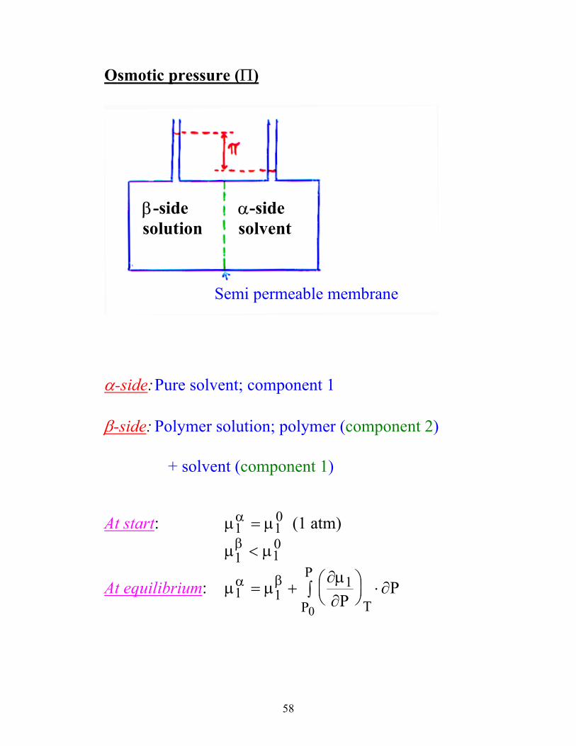
Osmotic pressure (Π)
β-side solution
α-side solvent
Semi permeable membrane
α-side: Pure solvent; component 1
β-side: Polymer solution; polymer (component 2)
+ solvent (component 1)
At start: µ µα1 1
0= (1 atm) µ µβ
1 10<
At equilibrium: µ µ∂µ∂
∂α β1 1
1
0
= +
⋅∫ PP
TP
P
59
From thermodynamics:
solvent) of (mol.vol. VP
1nn,T
1
21
=
∂∂µ
µ µα β
1 1 1 0− = −V P P( ) ∆ ΠG V1 1 1
01= − = − ⋅µ µβ
From equ. (26):
∆ Φ Φ ΦG R Tx
1 2 2 1 221 1 1
= ⋅ ⋅ − + −
⋅ + ⋅
ln( ) ε
Polynomial approximation:
ln( )12 32 222
23
− = − − − −Φ ΦΦ Φ
K
( )Φ2 1<<
Π ΦΦ Φ
ΦΦ
Φ= + + − + − ⋅
⋅
⋅2
22
23
22
1 22
12 3 xR TV
ε
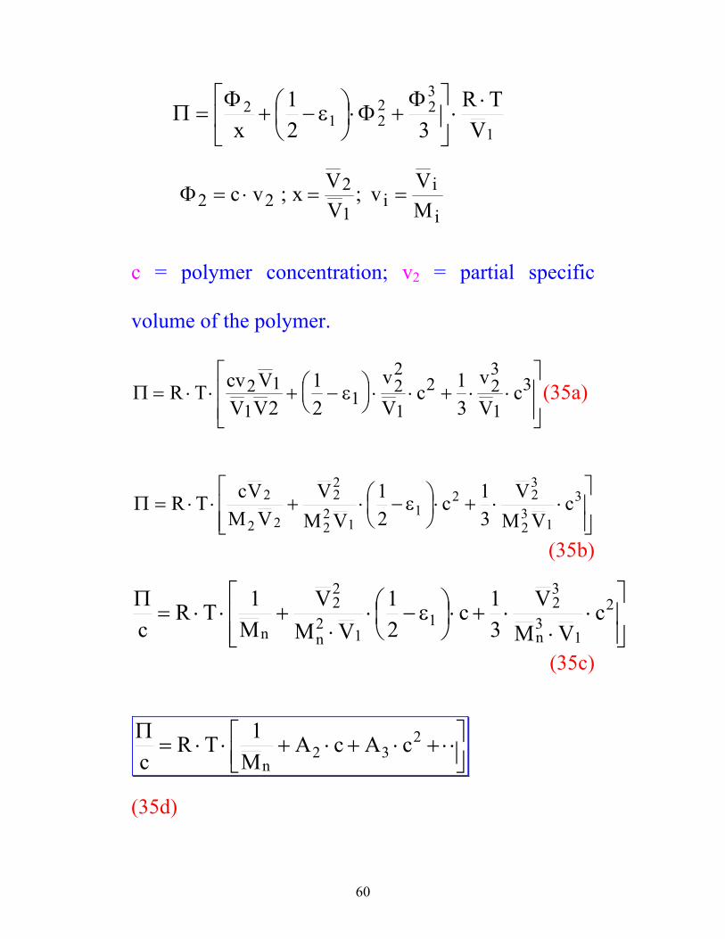
60
1
322
212
VTR
321
x⋅
⋅
Φ+Φ⋅
ε−+
Φ=Π
Φ2 22
1= ⋅ = =c x V
VVMi
i
iv v; ;
c = polymer concentration; v2 = partial specific
volume of the polymer.
Π = ⋅ ⋅ + −
⋅ ⋅ + ⋅ ⋅
R T cv VV V
vV
cvV
c2 11
122
12 2
3
13
212
13
ε (35a)
⋅⋅+⋅
ε−⋅+⋅⋅=Π 3
132
322
11
22
22
22
2 cVM
V31c
21
VMV
VMVcTR
(35b)
⋅
⋅⋅+⋅
ε−⋅
⋅+⋅⋅=
Π 2
13n
32
11
2n
22
nc
VMV
31c
21
VMV
M1TR
c(35c)
⋅⋅+⋅+⋅+⋅⋅=
Π 232
ncAcA
M1TR
c
(35d)
61
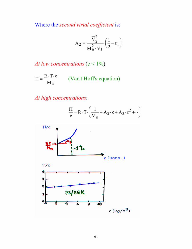
Where the second virial coefficient is:
AV
M Vn2
22
21
112
=⋅
⋅ −
ε
At low concentrations (c < 1%) Π =
⋅ ⋅R T cMn
(Van't Hoff's equation) At high concentrations:
Πc
R TM
A c A cn
= ⋅ ⋅ + ⋅ + ⋅ + ⋅⋅
12 3
2
62
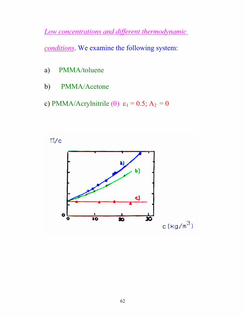
Low concentrations and different thermodynamic
conditions. We examine the following system:
a) PMMA/toluene b) PMMA/Acetone c) PMMA/Acrylnitrile (θ) ε1 = 0.5; A2 = 0
63
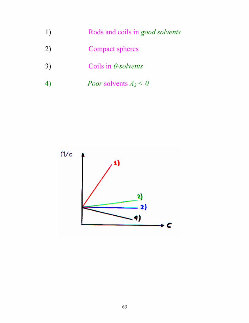
1) Rods and coils in good solvents
2) Compact spheres
3) Coils in θ-solvents
4) Poor solvents A2 < 0
64
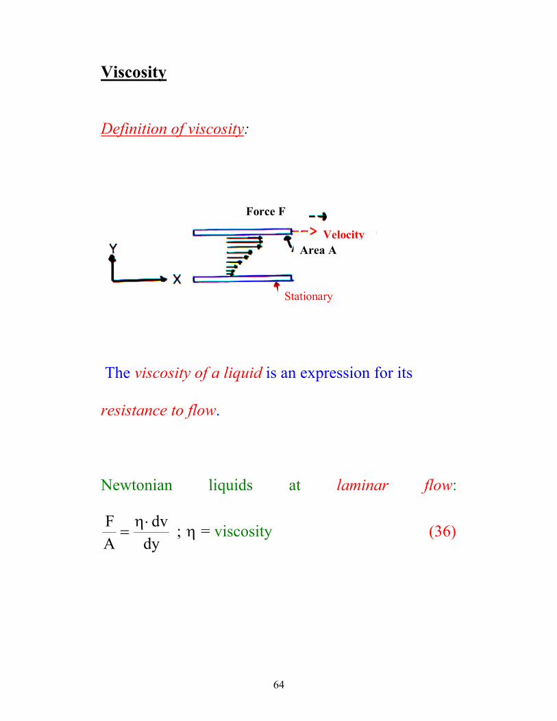
Viscosity
Definition of viscosity:
Force F
Velocity Area A
Stationary
The viscosity of a liquid is an expression for its
resistance to flow.
Newtonian liquids at laminar flow: FA
dvdy
=⋅η
η; = viscosity (36)
65
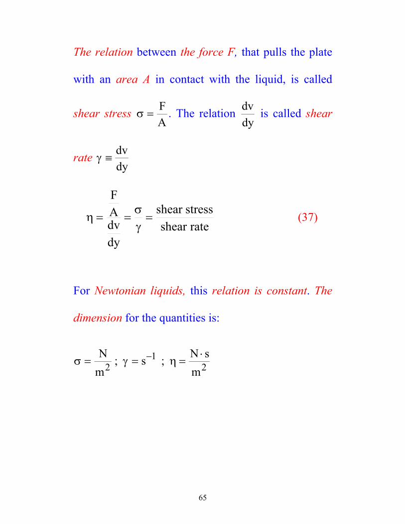
The relation between the force F, that pulls the plate
with an area A in contact with the liquid, is called
shear stress σ =FA
. The relation dvdy
is called shear
rate γ ≡ dvdy
rateshear
stressshear
dydvAF
=γσ
==η (37)
For Newtonian liquids, this relation is constant. The
dimension for the quantities is:
σ γ η= = =⋅−N
ms N s
m21
2; ;
66
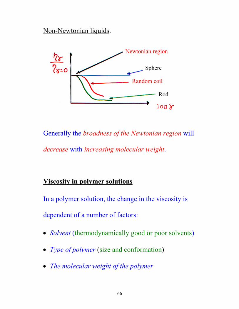
Non-Newtonian liquids. Newtonian region
Sphere
Random coil
Rod
Generally the broadness of the Newtonian region will
decrease with increasing molecular weight.
Viscosity in polymer solutions
In a polymer solution, the change in the viscosity is
dependent of a number of factors:
• Solvent (thermodynamically good or poor solvents)
• Type of polymer (size and conformation)
• The molecular weight of the polymer
67
• The polymer concentration
• Temperature
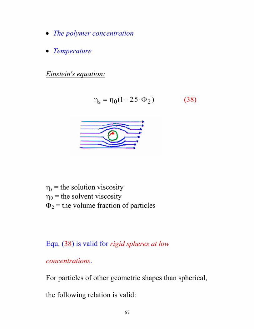
Einstein's equation: η ηs = + ⋅0 21 2 5( . )Φ (38)
ηs = the solution viscosity η0 = the solvent viscosity Φ2 = the volume fraction of particles
Equ. (38) is valid for rigid spheres at low
concentrations.
For particles of other geometric shapes than spherical,
the following relation is valid:
68
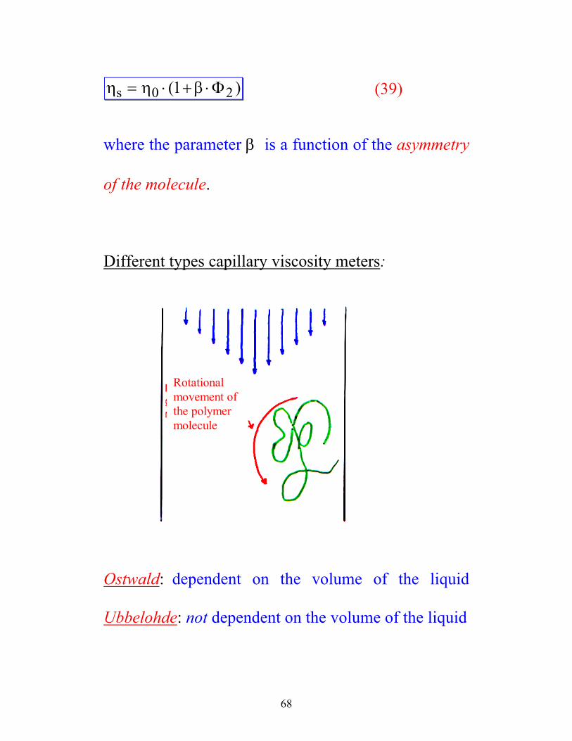
η η βs = ⋅ + ⋅0 21( )Φ (39)
where the parameter β is a function of the asymmetry
of the molecule.
Different types capillary viscosity meters:
Rotational movement of the polymer molecule
Ostwald: dependent on the volume of the liquid
Ubbelohde: not dependent on the volume of the liquid
69
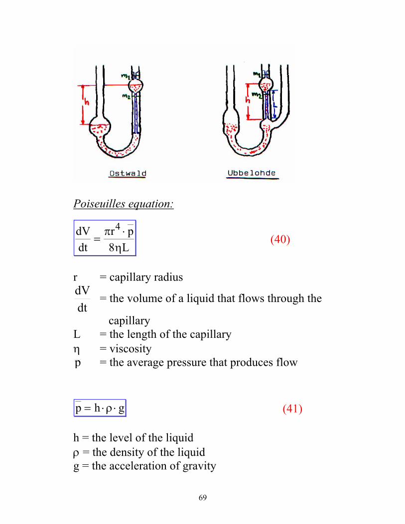
Poiseuilles equation:
dVdt
r pL
=⋅π
η
4
8 (40)
r = capillary radius
dtdV = the volume of a liquid that flows through the
capillary L = the length of the capillary η = viscosity p = the average pressure that produces flow
p h g= ⋅ ⋅ρ (41)
h = the level of the liquid ρ = the density of the liquid g = the acceleration of gravity
70
If we substitute equ. (41) in (40) and assumes
constant flow velocity we get:
ηπ ρ
=⋅ ⋅ ⋅ ⋅ ⋅
⋅ ⋅r h g t
L V
4
8 (42)
Equ. (42) is valid for Newtonian flow.
Reynolds number:R Vr tey =⋅ ⋅⋅ ⋅
<2 1000ρπ η
(Laminar flow)
Ret > 1000 (turbulent flow)
71
Determination of the intrinsic viscosity [η]
Relative viscosity: η ηη
ρρr
tt
= =⋅⋅0 0 0
0 indicates solvent.
In dilute solutions, ρ ≈ ρ0.
Specific viscosity: η ηsp rt t
t= − =
−1 0
0
Reduced viscosity: ηspc
Intrinsic viscosity: [ ]ηη
= ⋅ →lim ;spc
c 0
72
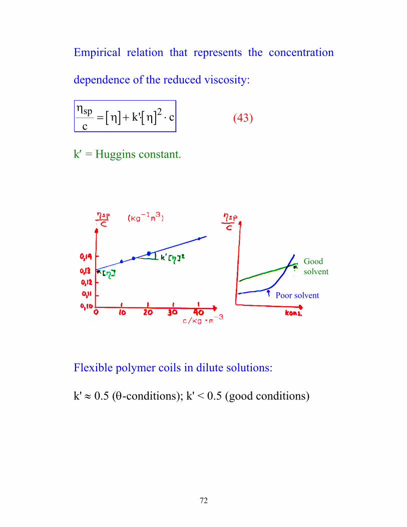
Empirical relation that represents the concentration
dependence of the reduced viscosity:
[ ] [ ]η
η ηspc
k c= + ⋅ ⋅' 2 (43)
k′ = Huggins constant.
Good solvent
Poor solvent
Flexible polymer coils in dilute solutions: k' ≈ 0.5 (θ-conditions); k' < 0.5 (good conditions)
73
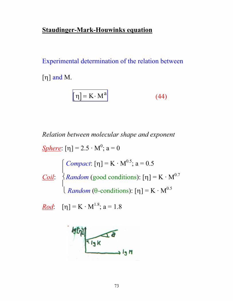
Staudinger-Mark-Houwinks equation
Experimental determination of the relation between
[η] and M.
[ ]η = ⋅K Ma (44)
Relation between molecular shape and exponent
Sphere: [η] = 2.5 · M0; a = 0
Compact: [η] = K · M0.5; a = 0.5 Coil: Random (good conditions): [η] = K · M0.7 Random (θ-conditions): [η] = K · M0.5 Rod: [η] = K · M1.8; a = 1.8
74
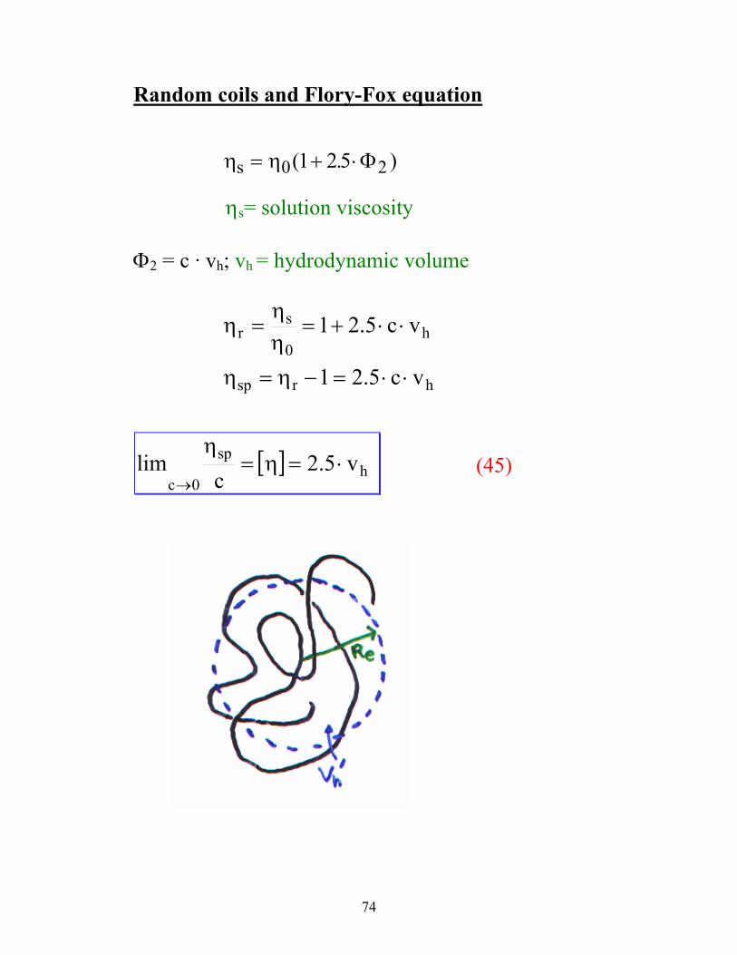
Random coils and Flory-Fox equation η ηs = + ⋅0 21 2 5( . )Φ
ηs= solution viscosity
Φ2 = c · vh; vh = hydrodynamic volume
hrsp
h0
sr
vc5.21
vc5.21
⋅⋅=−η=η
⋅⋅+=ηη
=η
[ ] hsp
0cv5.2
clim ⋅=η=
η
→ (45)
75
Let us assume that a random coil will behave as an
equivalent sphere with a radius Re:
Re = ψ · RG; ψ ≈ 0.8
The hydrodynamic volume for the particle is:
v Rh
G' =⋅ ⋅4
3
3 3π ψ
This is the hydrodynamic volume pr. sphere, but we
are interested in the hydrodynamic volume pr. weight
unit of the macromolecule.
v v NM
v R NM
hh A
hG A
=⋅
=⋅ ⋅ ⋅
⋅
'
43
3 3π ψ
76
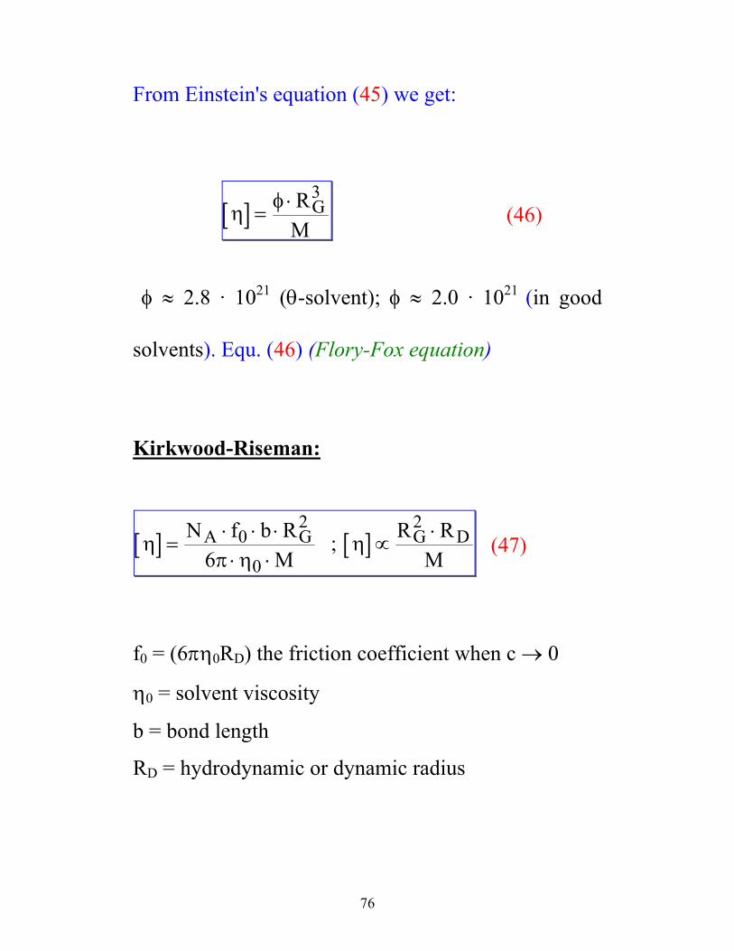
From Einstein's equation (45) we get:
[ ]η φ= ⋅RM
G3
(46)
φ ≈ 2.8 · 1021 (θ-solvent); φ ≈ 2.0 · 1021 (in good
solvents). Equ. (46) (Flory-Fox equation)
Kirkwood-Riseman:
[ ] [ ]ηπ η
η=⋅ ⋅ ⋅⋅ ⋅
∝⋅N f b R
MR R
MA G G D0
2
0
2
6; (47)
f0 = (6πη0RD) the friction coefficient when c → 0
η0 = solvent viscosity
b = bond length
RD = hydrodynamic or dynamic radius
77
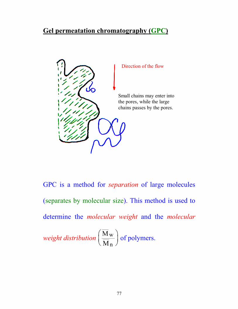
Gel permeatation chromatography (GPC)
Direction of the flow
Small chains may enter into the pores, while the large chains passes by the pores.
GPC is a method for separation of large molecules
(separates by molecular size). This method is used to
determine the molecular weight and the molecular
weight distribution MM
w
n
of polymers.
78
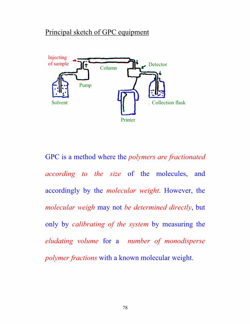
Principal sketch of GPC equipment
Injecting of sample
Solvent
Pump
Column Detector
Printer
Collection flask
GPC is a method where the polymers are fractionated
according to the size of the molecules, and
accordingly by the molecular weight. However, the
molecular weigh may not be determined directly, but
only by calibrating of the system by measuring the
eludating volume for a number of monodisperse
polymer fractions with a known molecular weight.
79
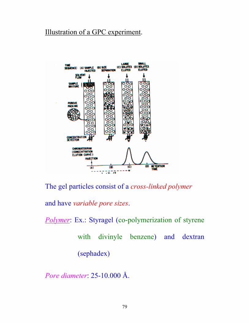
Illustration of a GPC experiment.
The gel particles consist of a cross-linked polymer
and have variable pore sizes.
Polymer: Ex.: Styragel (co-polymerization of styrene
with divinyle benzene) and dextran
(sephadex)
Pore diameter: 25-10.000 Å.
80
The stationary phase of the column: The gel particles
included the liquid that is bond inside the pores.
The mobile phase of the column: The eludating
sample that flows through the column between the gel
particles.
The sample with polymer: A small volume is injected
at the top of the column.
Detector: UV-absorption, refractive index
(differential refractometer).
Retention time: The time that a certain fraction is in
the column.
81
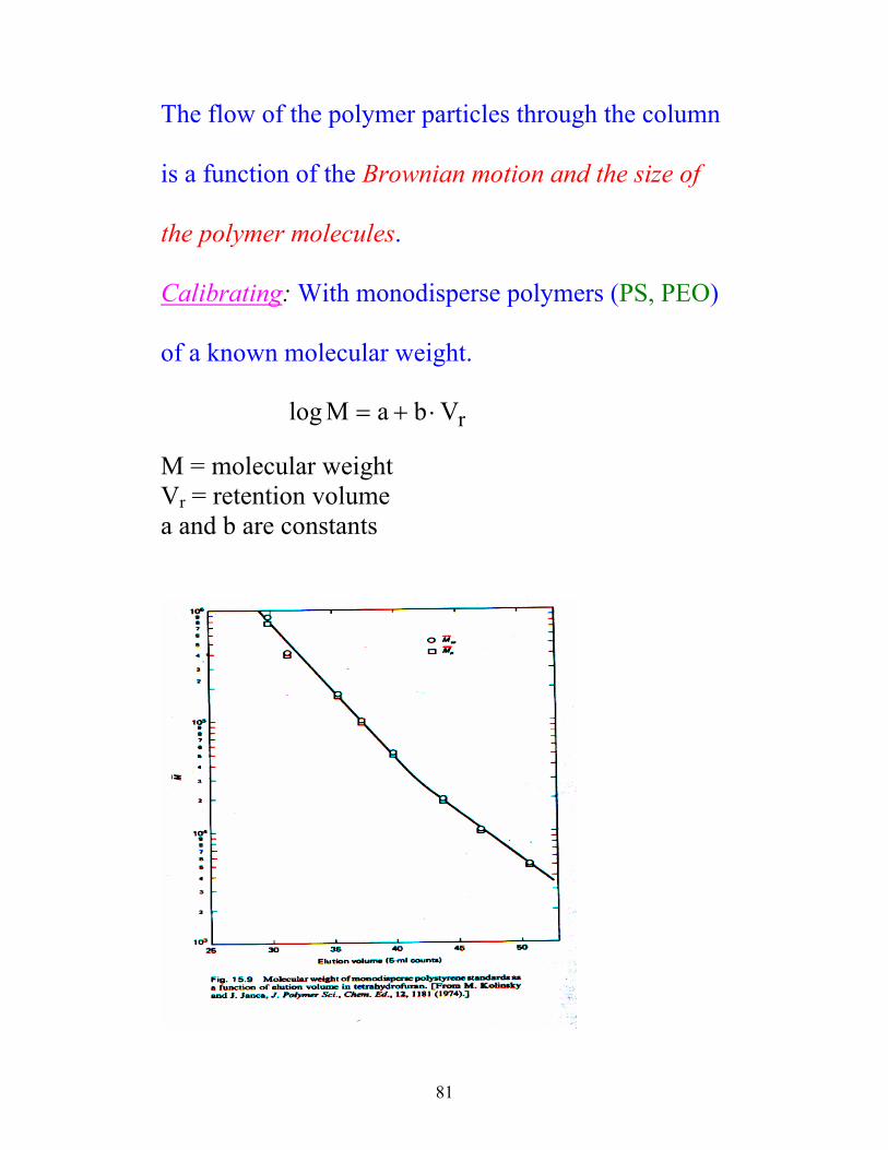
The flow of the polymer particles through the column
is a function of the Brownian motion and the size of
the polymer molecules.
Calibrating: With monodisperse polymers (PS, PEO)
of a known molecular weight.
log M a b Vr= + ⋅ M = molecular weight Vr = retention volume a and b are constants
82
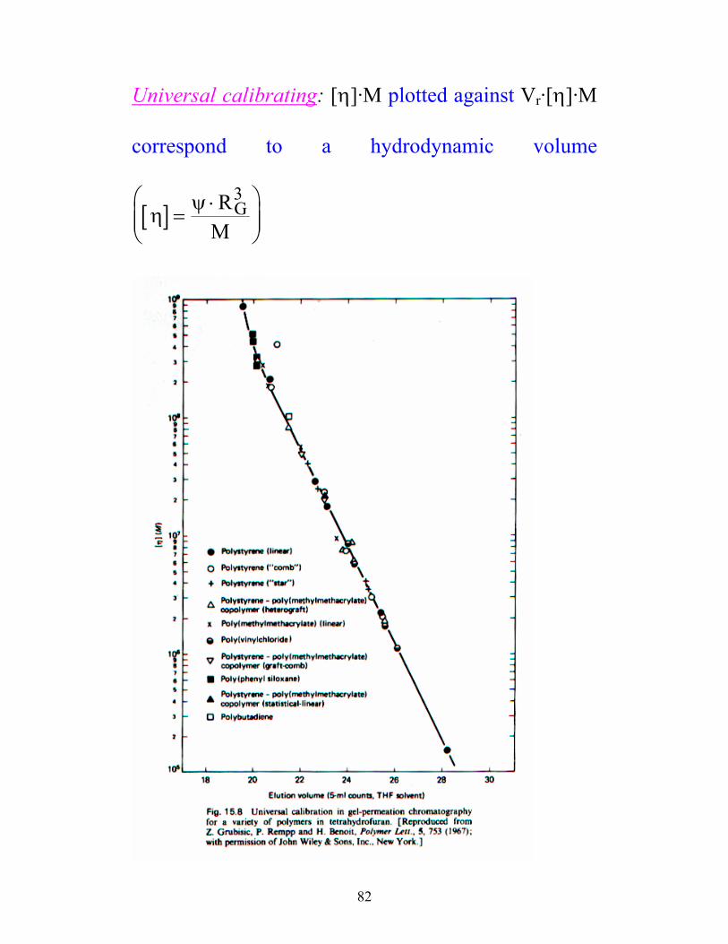
Universal calibrating: [η]·M plotted against Vr·[η]·M
correspond to a hydrodynamic volume
[ ]η ψ=
⋅
RM
G3
83
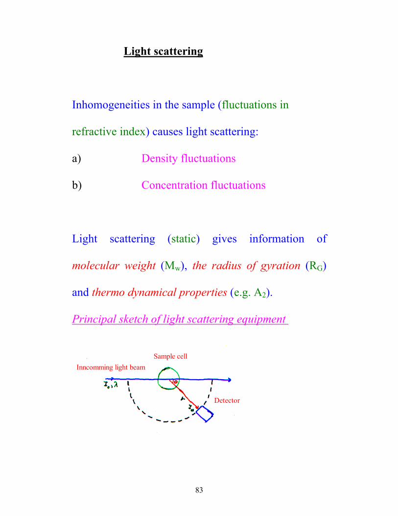
Light scattering
Inhomogeneities in the sample (fluctuations in
refractive index) causes light scattering:
a) Density fluctuations
b) Concentration fluctuations
Light scattering (static) gives information of
molecular weight (Mw), the radius of gyration (RG)
and thermo dynamical properties (e.g. A2).
Principal sketch of light scattering equipment
Inncomming light beam Sample cell
Detector
84
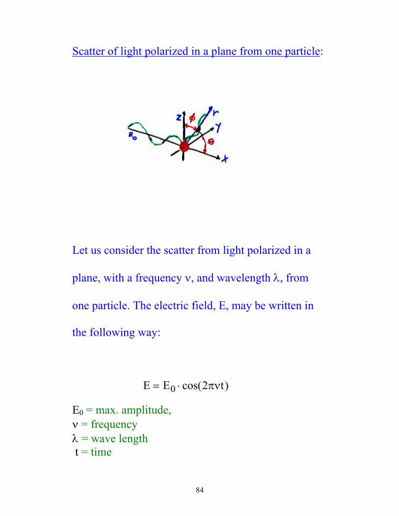
Scatter of light polarized in a plane from one particle:
Let us consider the scatter from light polarized in a
plane, with a frequency ν, and wavelength λ, from
one particle. The electric field, E, may be written in
the following way:
E E t= ⋅0 2cos( )πν
E0 = max. amplitude, ν = frequency λ = wave length t = time
85
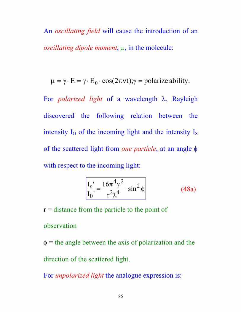
An oscillating field will cause the introduction of an
oscillating dipole moment, µ, in the molecule:
ability. polarize );t2cos(EE 0 =γπν⋅⋅γ=⋅γ=µ
For polarized light of a wavelength λ, Rayleigh
discovered the following relation between the
intensity IO of the incoming light and the intensity IS
of the scattered light from one particle, at an angle φ
with respect to the incoming light:
II rs ''
sin0
4 2
2 4216
= ⋅π γ
λφ (48a)
r = distance from the particle to the point of
observation
φ = the angle between the axis of polarization and the
direction of the scattered light.
For unpolarized light the analogue expression is:
86
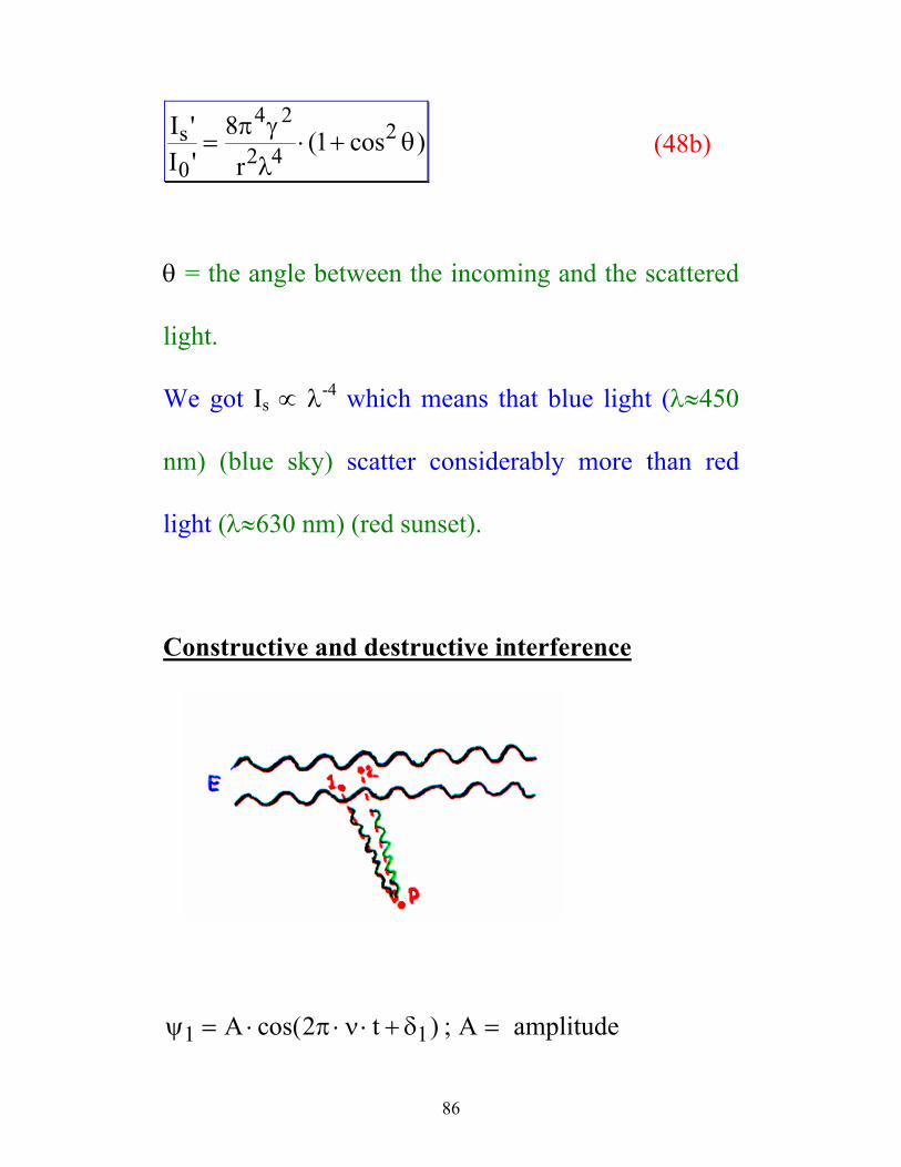
II rs ''
( cos )0
4 2
2 428 1= ⋅ +
π γ
λθ (48b)
θ = the angle between the incoming and the scattered
light.
We got Is ∝ λ-4 which means that blue light (λ≈450
nm) (blue sky) scatter considerably more than red
light (λ≈630 nm) (red sunset).
Constructive and destructive interference
ψ π ν δ1 12= ⋅ ⋅ ⋅ + =A t Acos( ) ; amplitude
87
ψ π ν δ2 22= ⋅ ⋅ ⋅ +A tcos( )
δ1 and δ2 represents the phase shift from particle 1 and
2, respectively. (The particles have unequal distance
from the source of radiation and additionally the
distance between the particles and the detector is
unequal.)
The collected succession of waves at P is:
ψ ψ ψ= +1 2
ψ π ν δ π ν δ= ⋅ ⋅ ⋅ + + ⋅ ⋅ ⋅ +A t A tcos( ) cos( )2 21 2
∆δ = δ2 - δ1 = n1 · 180o; n1 is an odd number multiple
of 180°, the succession of waves cancels each other
out (destructive interference).
∆δ = 0, or a multiple of 360°, the succession of waves
will amplify each other (constructive interference).
88
If the two particles move independent of each other
(ideal gas), all ∆δ will be equal probable → the effect
of the interference will at average equal 0.
At the observation point:
I I Is s s= +, ,1 2
Solutions of macromolecules
Rayleigh scattering:
RG <λ20
We will now regard the excess light scattering that are
due to particles dissolved in the liquid.
Fluctuation theory (Einstein): One imagines that the
liquid is divided into volume elements that are less
than the wavelength of the light.
89
The volume elements have a fluctuating
concentration of macromolecules. These
concentration fluctuations must necessarily be
dependent of the size of the macromolecules
( )M Rw G, and interactions in the system (A2:
thermodynamic properties).
Ideal solution: Classical electro magnetic theory:
n n N202 4− = ⋅ ⋅π γ (49)
nandn;unitvolumeparticlesofnumberN 0= is the
refractive index of solvent and solution, respectively.
90
( ) ( )n n n n N− ⋅ + = ⋅ ⋅0 0 4π γ
γπ
=+
⋅−
⋅n n n n
ccN
0 04
(1) (2) (3)
(1) In a dilute solution: n + n0 ≈ 2n0
(2) dndc
refractive index increment
(3) N c NM
A= ⋅ (50)
γπ
= ⋅ ⋅⋅
n dndc
MN A
0 2 (51)
We put this into Rayleigh's equ. (48b):
II
n dndc
Mr N
n dndc
Mr N
s
A
A
′= ⋅ ⋅ ⋅
+=
= ⋅ ⋅
⋅ ⋅+
0
402 2 2
2
2 4 2 2
202
22
2
4 2 2
8 12
2 1
πθ
λ π
πθ
λ
( ) cos( )
cos
(52)
91
Is’ is the scatter from one particle, but we want to
know the scatter from N particles ( N c NM
A= ⋅ ):
( )II
n dndc
c M
r Ns
A0
202
2 2
4 221
= ⋅ ⋅
⋅+ ⋅ ⋅
⋅ ⋅π
θ
λ
cos (53)
II
r R n dndc N
c Ms
A0
2
22
02
2
412 1⋅
+= = ⋅ ⋅
⋅ ⋅ ⋅cos θ
πλ
θ
Rθ = reduced scattered intensity
solventsolution RRR θθθ −=
K n dndc NA
= ⋅ ⋅
⋅2 1202
2
4πλ
K = constant for a given polymer system
92
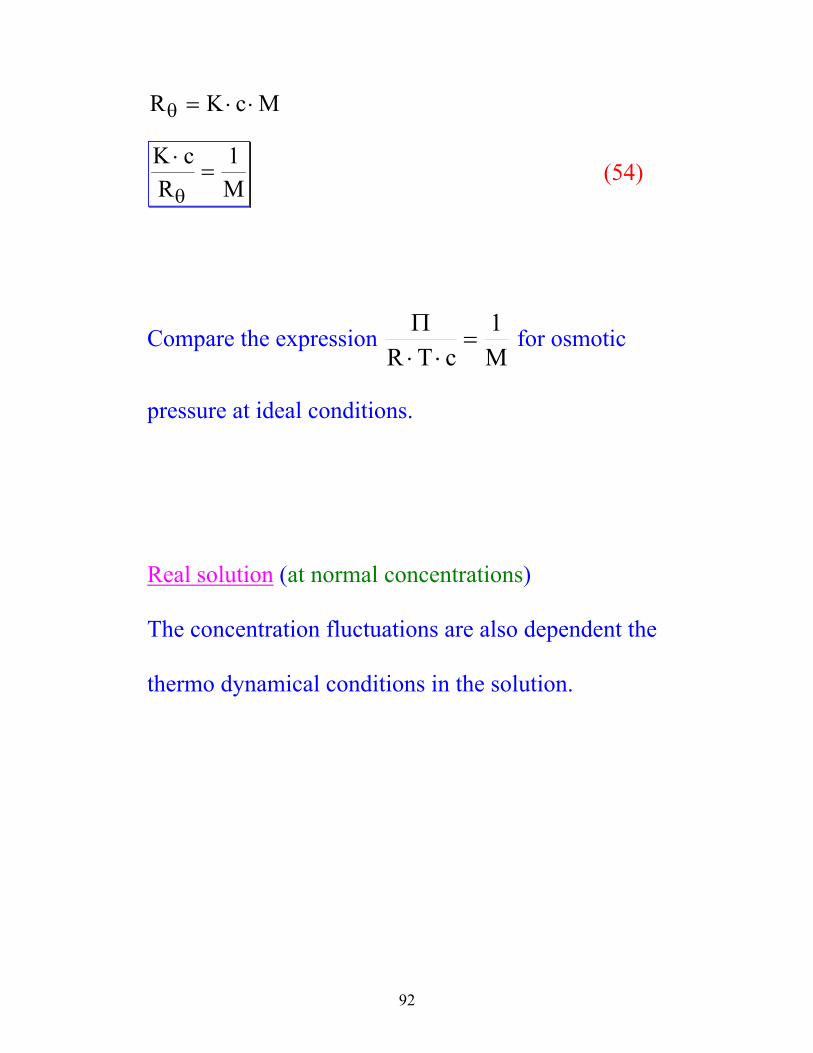
R K c Mθ = ⋅ ⋅
K cR M⋅
=θ
1 (54)
Compare the expression M1
cTR=
⋅⋅Π for osmotic
pressure at ideal conditions.
Real solution (at normal concentrations)
The concentration fluctuations are also dependent the
thermo dynamical conditions in the solution.
93
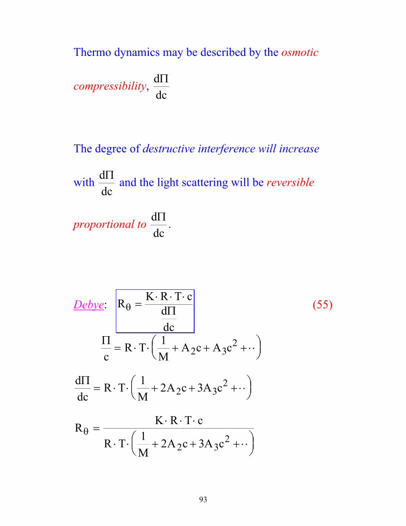
Thermo dynamics may be described by the osmotic
compressibility, ddcΠ
The degree of destructive interference will increase
with ddcΠ and the light scattering will be reversible
proportional to ddcΠ .
Debye: RK R T c
ddc
θ =⋅ ⋅ ⋅Π (55)
Πc
R TM
A c A c= ⋅ ⋅ + + + ⋅⋅
12 3
2
ddc
R TM
A c A cΠ= ⋅ ⋅ + + + ⋅⋅
1 2 32 32
R K R T c
R TM
A c A cθ =
⋅ ⋅ ⋅
⋅ ⋅ + + + ⋅⋅
1 2 32 32
94
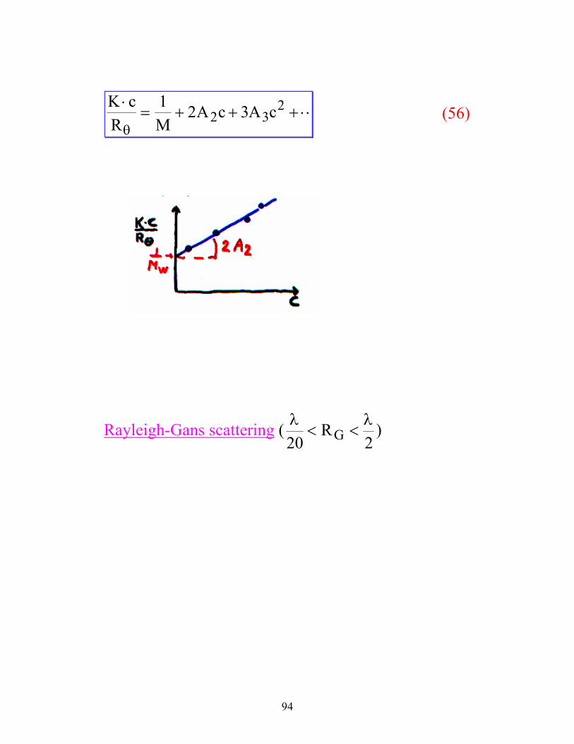
K cR M
A c A c⋅= + + + ⋅⋅
θ
1 2 32 32
(56)
Rayleigh-Gans scattering ( λ λ20 2
< <RG )
95
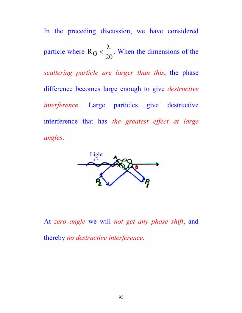
In the preceding discussion, we have considered
particle where RG <λ20
. When the dimensions of the
scattering particle are larger than this, the phase
difference becomes large enough to give destructive
interference. Large particles give destructive
interference that has the greatest effect at large
angles.
Light
At zero angle we will not get any phase shift, and
thereby no destructive interference.
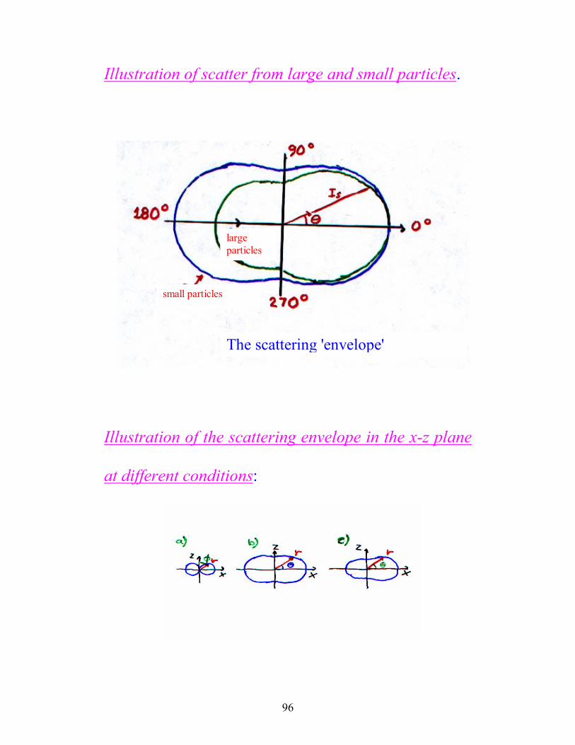
96
Illustration of scatter from large and small particles.
large particles
small particles
The scattering 'envelope'
Illustration of the scattering envelope in the x-z plane
at different conditions:
97
a) Rayleigh-scattering (Rθλ
<20
) of light polarized in
a plane
b) Rayleigh-scattering (Rθλ
<20
) of unpolarized light
c) Rayleigh-Gans-scattering ( λ λθ20 2
< <R ) of
unpolarized light
The distribution of the angle of the scattered light is
dependent of several different factors:
a) the size of the particle
b) the shape of the particle
c) interactions between the particles
d) the size distribution of the particles
98
At low scattering angles, θ, and at low
concentrations, the angular dependency is
independent of the shape of the particle and only
dependent on the average radius of gyration of the
particle.
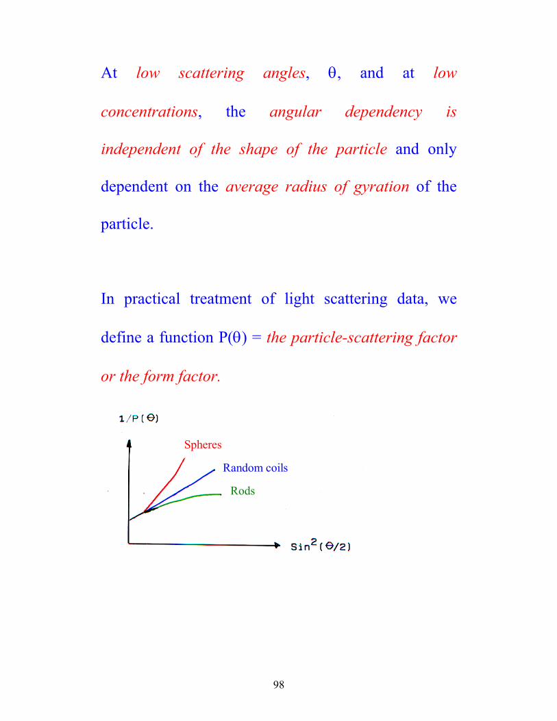
In practical treatment of light scattering data, we
define a function P(θ) = the particle-scattering factor
or the form factor.
Spheres
Random coils
Rods
99
)scattering-Rayleigh produced hadit if particle same (the)(Rparticle)(real)(R)(P
θθ
=θ
Rayleighreal )R()(P)R(
0for 1)(P and 0 when 1)(P
θθ ⋅θ=
>θ<θ→θ→θ
From equ. (56)
K cR P M
A c A c⋅= ⋅ + ⋅ + ⋅ + ⋅⋅
θ θ
1 1 2 32 32 (57)
θ θ
πθ
λ→
= +
⋅ ⋅ ⋅
⋅0
2 2 2
21 1
162
3Lim
P
RG
( )
sin (58)
We may now write the light scattering equation (57)
in this way
K cR
R
MA c
G⋅= +
⋅ ⋅ ⋅
⋅
⋅ + ⋅
θ
πθ
λ1
162
3
1 2
2 2 2
2 2
sin (59)
100
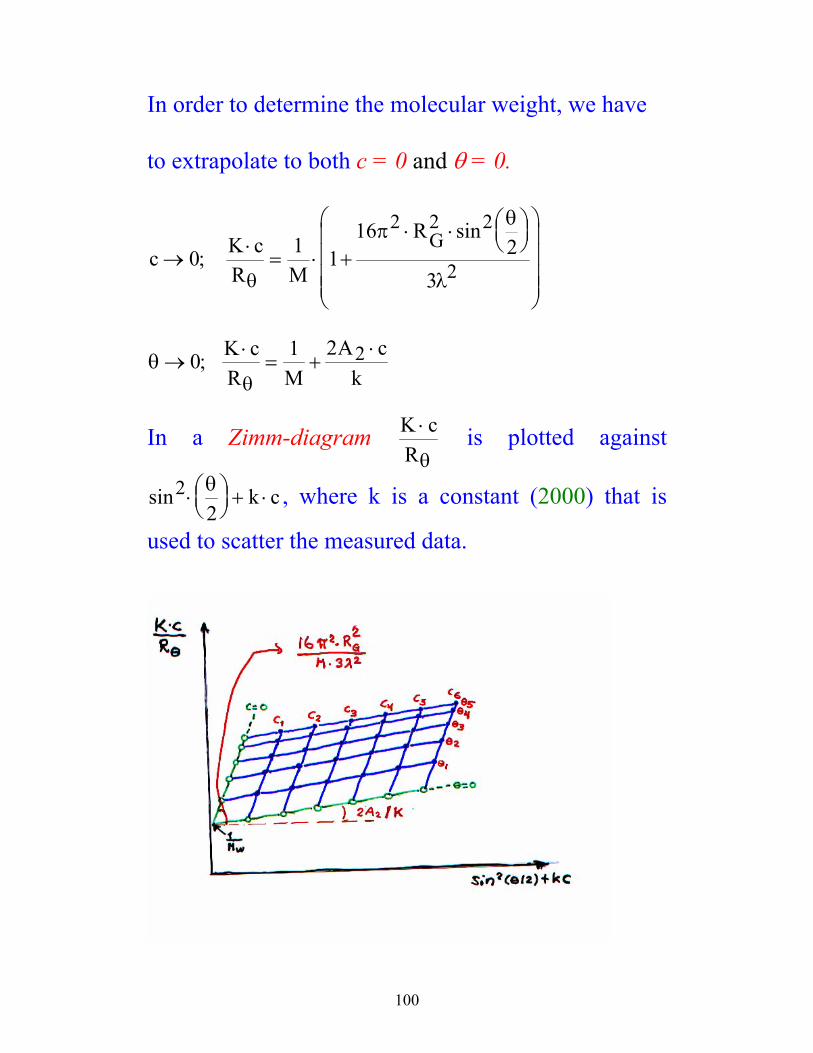
In order to determine the molecular weight, we have
to extrapolate to both c = 0 and θ = 0.
c K cR M
RG→
⋅= ⋅ +
⋅ ⋅
0 1 116
23
2 2 2
2;sin
θ
πθ
λ
θθ
→⋅
= +⋅0 1 2 2; K c
R MA c
k
In a Zimm-diagram K cR⋅
θ is plotted against
sin22
⋅
+ ⋅
θ k c , where k is a constant (2000) that is
used to scatter the measured data.
101
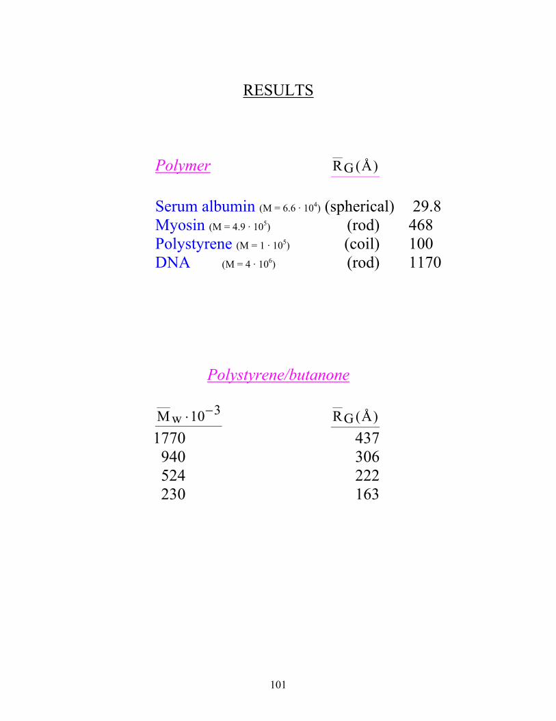
RESULTS
Polymer R ÅG ( ) Serum albumin (M = 6.6 · 104) (spherical) 29.8 Myosin (M = 4.9 · 105) (rod) 468 Polystyrene (M = 1 · 105) (coil) 100 DNA (M = 4 · 106) (rod) 1170
Polystyrene/butanone
M w ⋅ −10 3 R ÅG ( ) 1770 437 940 306 524 222 230 163
102
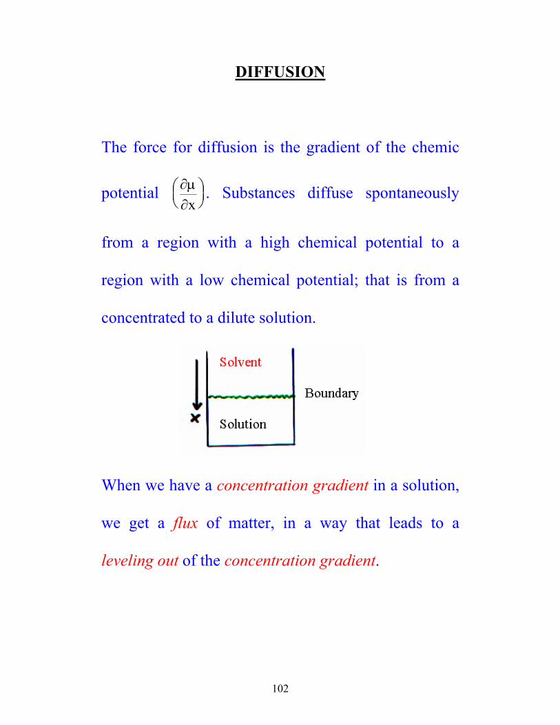
DIFFUSION
The force for diffusion is the gradient of the chemic
potential ∂µ∂x
. Substances diffuse spontaneously
from a region with a high chemical potential to a
region with a low chemical potential; that is from a
concentrated to a dilute solution.
When we have a concentration gradient in a solution,
we get a flux of matter, in a way that leads to a
leveling out of the concentration gradient.
103
J D cx
= − ⋅∂∂
(Fick’s law) (60)
( )12 smkgfluxJ −− ⋅⋅= D = the diffusion coefficient (m2·s-1)
)mkg.(consc 3=
In order to eliminate the flux, we may use the
continuity equation:
∂∂
∂∂
ct
Jx
= − (61)
Combination of (60) and (61) give:
∂∂
∂
∂
ct
D c
x=
2
2 (Fick’s second law) (62)
104
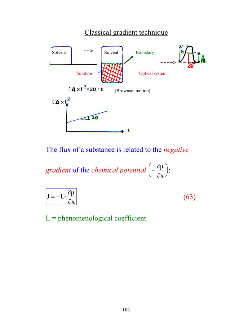
Classical gradient technique equalize
Solvent Solvent
Solution
Boundary
Optical system
(Brownian motion)
The flux of a substance is related to the negative
gradient of the chemical potential −
∂µ∂x
:
J Lx
= − ⋅∂µ∂
(63)
L = phenomenological coefficient
105
Ideal solutions:
µ µ
∂µ∂
∂µ∂
∂∂
∂∂
= + ⋅ ⋅
= ⋅ =⋅
⋅
0 R T c
x ccx
R Tc
cx
ln
Combination with equ. (63) gives:
J L R Tc
cx
= −⋅ ⋅
⋅∂∂
(64)
The flux may also be expressed in another way: J c v L
x= ⋅ = − ⋅
∂µ∂
v = velocity
c = concentration
In diffusion, the force (pr. mol) − ∂µ∂x
is balanced by
the frictional force
A0fr
0fr
Nvfmol) (pr. F
vfmolecule)(pr. F
⋅⋅=
⋅=
106
f0= the frictional coefficient
c v L f v N L cf NA
A⋅ = ⋅ ⋅ ⋅ → =
⋅00
(65)
We may now write equ. (64) in this way:
J c R Tf N c
cx
R Tf N
cxA A
= −⋅ ⋅⋅ ⋅
⋅ = −⋅⋅
⋅0 0
∂∂
∂∂
(66)
Compare equ. (60) with equ. (66):
c D R Tf NA
→ =⋅⋅
0 00
(67)
when c >> 0
( )D M v c cf NA
= ⋅ − ⋅ ⋅⋅
1 2
∂π∂ (68)
( ) ( )D R TN f
v c A M c A M cA
=⋅⋅⋅ − ⋅ ⋅ + ⋅ ⋅ + ⋅ ⋅ + ⋅1 1 2 32 2 3
2 (69)
107
⋅
⋅⋅
=factoricHydrodynamA fN
TRD Q(c)Thermodynamic factor
(69a)
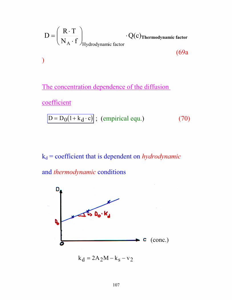
The concentration dependence of the diffusion
coefficient
( )D D k cd= + ⋅0 1 ; (empirical equ.) (70)
kd = coefficient that is dependent on hydrodynamic
and thermodynamic conditions
(conc.)
k A M k vd s= − −2 2 2
108
ULTRA CENTRIFUGATION (Svedberg)
Velocity centrifugation (50.000-60.000 r.p.m.) gives
hydrodynamic information
Equilibrium centrifugation (5.000-6.000 r.p.m.) gives
thermodynamic information
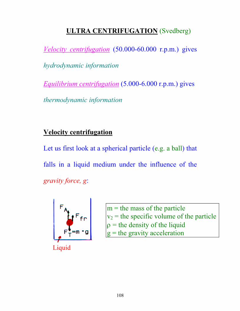
Velocity centrifugation
Let us first look at a spherical particle (e.g. a ball) that
falls in a liquid medium under the influence of the
gravity force, g:
Liquid
m = the mass of the particle v2 = the specific volume of the particle ρ = the density of the liquid g = the gravity acceleration
109
fr2
frAT
frAT
Fgvmgm
FFF
0a ,short timeaafter ;amFFF
+⋅ρ⋅⋅=⋅
+=
≈⋅=−−
m·v2 represents the volume of displaced liquid
Ffr = m·g(1-v2·ρ) represents the upwards pressure
m MN
F f vA
fr= = ⋅;
f = the friction coefficient, that is dependent of the
size and shape of the particles, and the viscosity of the
liquid.
( )f v MN
v gA
⋅ = ⋅ − ⋅1 2ρ (71)
110
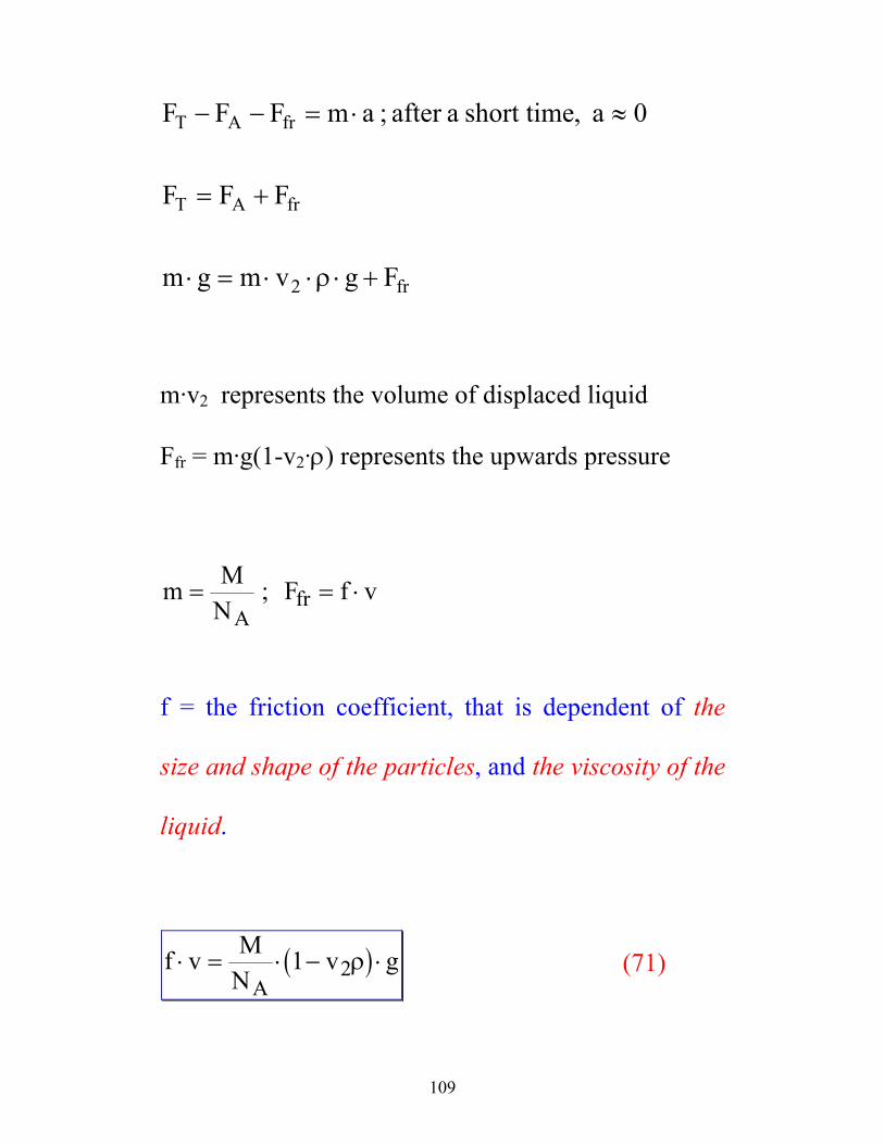
Macromolecules are far too small particles to
sediment in the earth's gravitational field, one
therefore need to apply a centrifugal field (ultra
centrifuge) in order to get the molecules to sediment.
Ω = Angular velocity
Fs = Sentrifug. force Solution
In a centrifugal field, g is replaced by Ω2·r
(200.000.g), where Ω is the angular velocity and r is
the distance from the rotor axis. Equ. (71) may now
be written as:
( )f v MN
v rA
⋅ = ⋅ − ⋅ ⋅ ⋅1 22ρ Ω (72)
Ex.
111
60 000 r.p.m. Ω2·r=(2π·1000)2·(6 cm)=2.38·106 cm·s-2 Svedberg introduced a parameter that is called the
sedimentation coefficient, S:
S vr
v drdt
=⋅
=Ω2 ; ( ) (73)
A combination of equ. (72) and (73), and when we
additionally look at the situation when c → 0:
S M vN fA
02 00
1=
⋅ − ⋅⋅
( )ρ (74)
112
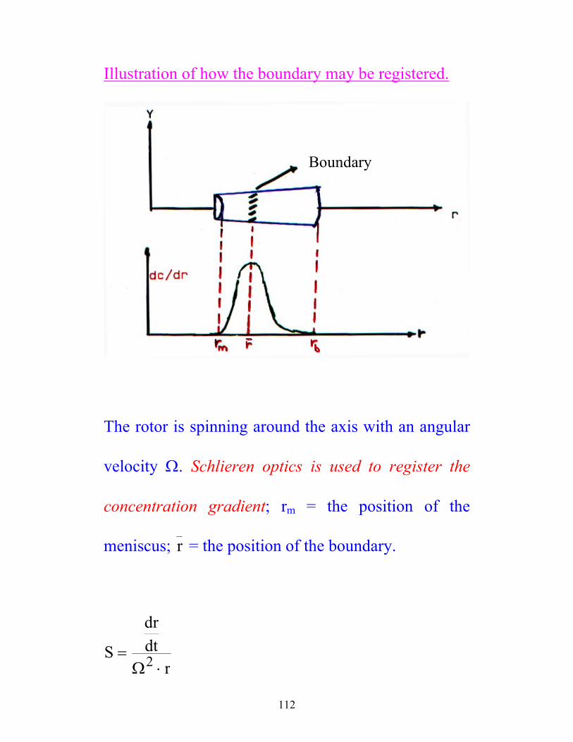
Illustration of how the boundary may be registered.
Boundary
The rotor is spinning around the axis with an angular
velocity Ω. Schlieren optics is used to register the
concentration gradient; rm = the position of the
meniscus; r = the position of the boundary.
S
drdt
r=
⋅Ω2
113
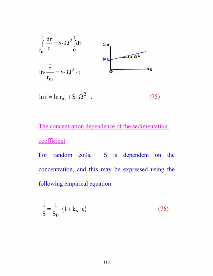
drr
S dtr
r t
m∫ = ⋅ ∫Ω2
0
ln⋅ = ⋅ ⋅r
rS t
mΩ2
ln lnr r S tm= + ⋅ ⋅Ω2 (75)
The concentration dependence of the sedimentation
coefficient
For random coils, S is dependent on the
concentration, and this may be expressed using the
following empirical equation:
( )1 1 10S S
k cs= ⋅ + ⋅ (76)
114
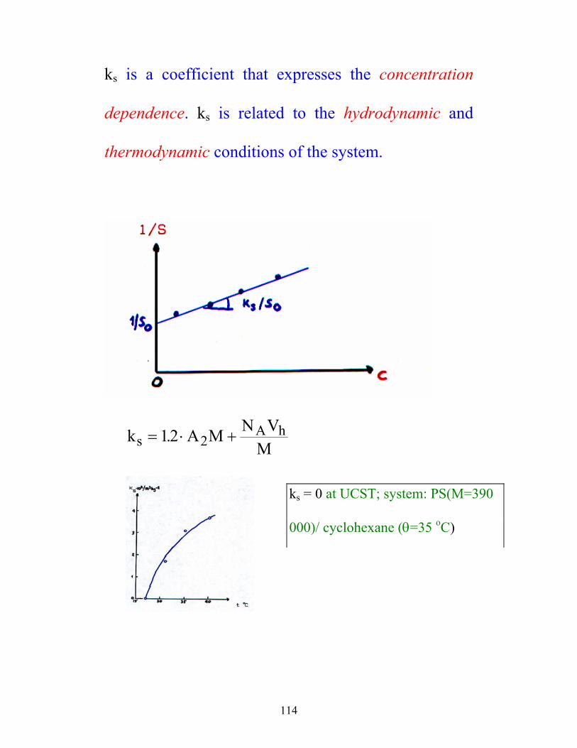
ks is a coefficient that expresses the concentration
dependence. ks is related to the hydrodynamic and
thermodynamic conditions of the system.
k A M N VMsA h= ⋅ +12 2.
ks = 0 at UCST; system: PS(M=390
000)/ cyclohexane (θ=35 oC)
115
In order to determine the molecular weight in equ..
(74), we need to know f0. One may determine f0. from
diffusion measurements (equ. (67)). D R TN fA
00
=⋅⋅
.
By combining equ. (67) and (74), we get the Svedberg
equation:
( )M S R T
D v=
⋅ ⋅− ⋅
00 2 01 ρ
(77)
Equilibrium centrifugation
If we let the rotor rotate at a relatively slow speed
(5.000-6.000 r.p.m.) we may get equilibrium in the
cell, so no net sedimentation is taking place. This
usually takes a long time (several days).
116
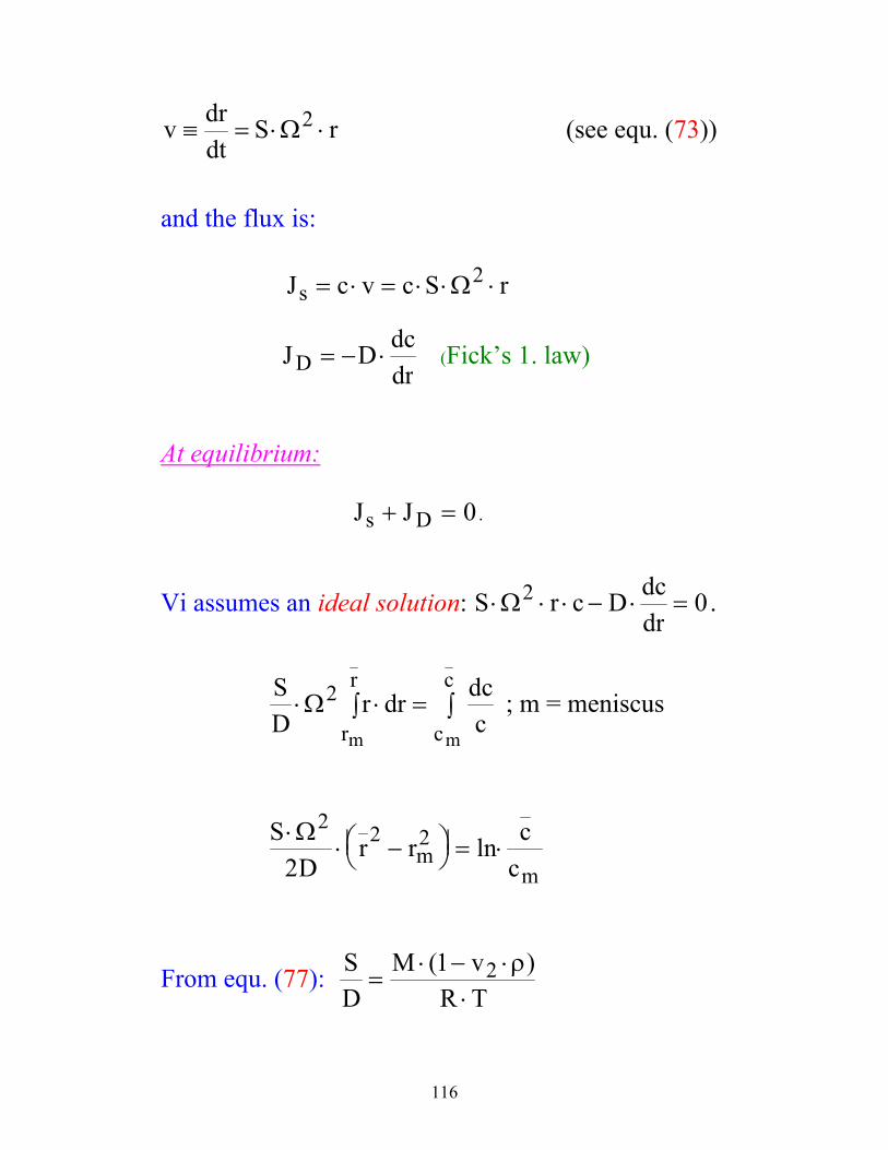
v drdt
S r≡ = ⋅ ⋅Ω2 (see equ. (73))
and the flux is:
J c v c S rs = ⋅ = ⋅ ⋅ ⋅Ω2
J D dcdrD = − ⋅ (Fick’s 1. law)
At equilibrium: J Js D+ = 0.
Vi assumes an ideal solution: S r c D dcdr
⋅ ⋅ ⋅ − ⋅ =Ω2 0.
SD
r dr dccr
r
c
c
m m
⋅ ⋅∫ = ∫Ω2 ; m = meniscus
S
Dr r c
cmm
⋅⋅ −
= ⋅
Ω2 2 22
ln
From equ. (77): SD
M vR T
=⋅ − ⋅
⋅( )1 2 ρ
117
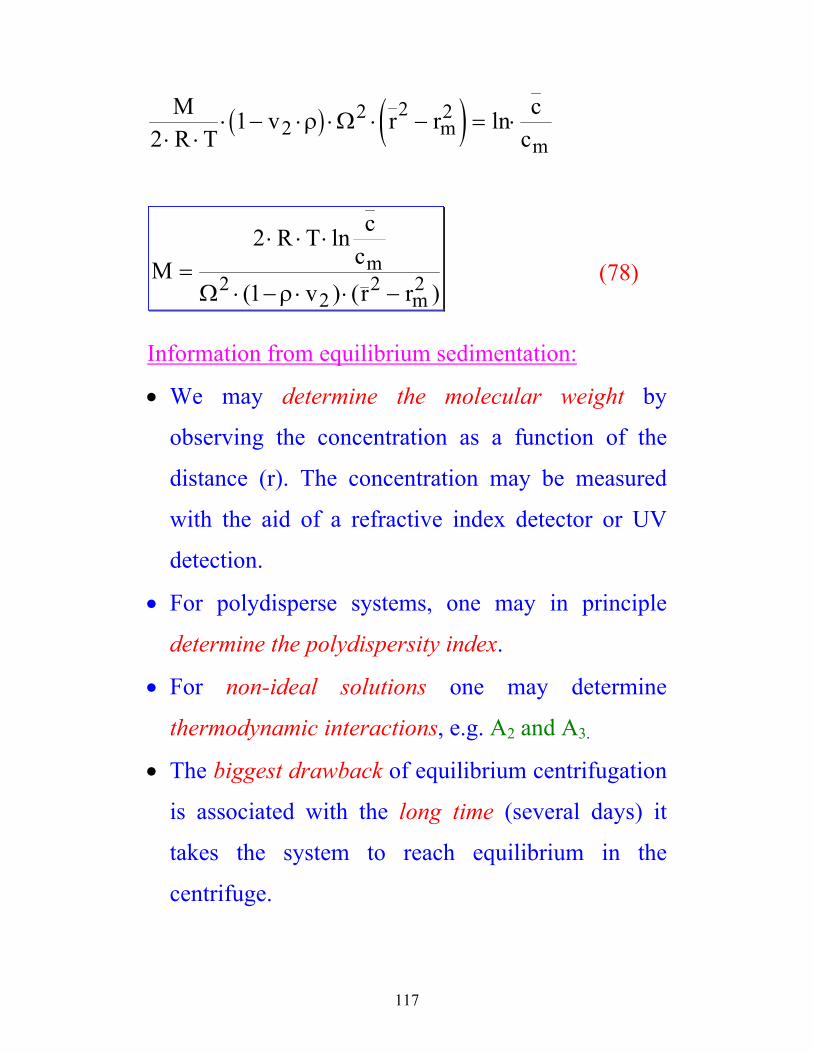
( ) ( )MR T
v r r ccm
m21 2
2 2 2⋅ ⋅
⋅ − ⋅ ⋅ ⋅ − = ⋅ρ Ω ln
MR T c
cv r r
m
m=
⋅ ⋅ ⋅
⋅ − ⋅ ⋅ −
2
122
2 2
ln
( ) ( )Ω ρ (78)
Information from equilibrium sedimentation:
• We may determine the molecular weight by
observing the concentration as a function of the
distance (r). The concentration may be measured
with the aid of a refractive index detector or UV
detection.
• For polydisperse systems, one may in principle
determine the polydispersity index.
• For non-ideal solutions one may determine
thermodynamic interactions, e.g. A2 and A3.
• The biggest drawback of equilibrium centrifugation
is associated with the long time (several days) it
takes the system to reach equilibrium in the
centrifuge.
118
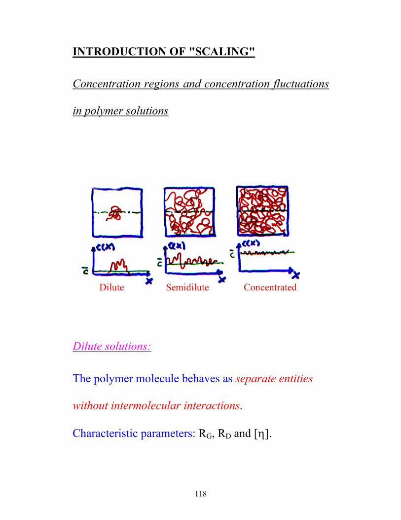
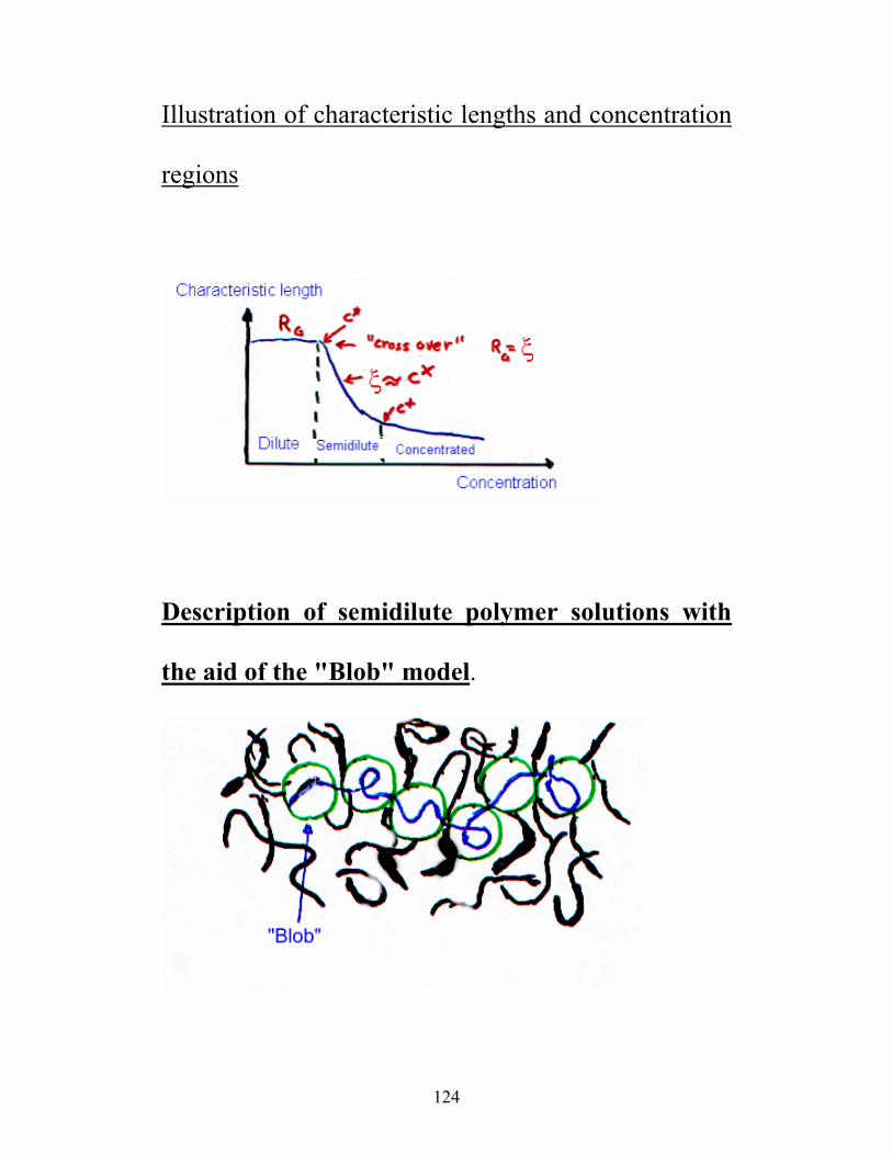
INTRODUCTION OF "SCALING" Concentration regions and concentration fluctuations
in polymer solutions
Dilute Semidilute Concentrated
Dilute solutions: The polymer molecule behaves as separate entities
without intermolecular interactions.
Characteristic parameters: RG, RD and [η].
119
Static parameter:
R K MG G G= ⋅ β
βG = 0.59 (good conditions) βG = 0.50 (θ-conditions) Dynamical parameters:
D R TN fA
00
=⋅⋅
D k Tf
k TRD
00 06
=⋅
=⋅
⋅ ⋅π η
Stoke’s law: f R R K MD D D D0 06= ⋅ ⋅ = ⋅π η β;
At θ-conditions, we always have βG = βD.
At good conditions: βG = βD only when M → ∞,
otherwise: βD < βG and the numerical value of βD is
dependent on the considered molecular weight region.
Intrinsic viscosity:
120
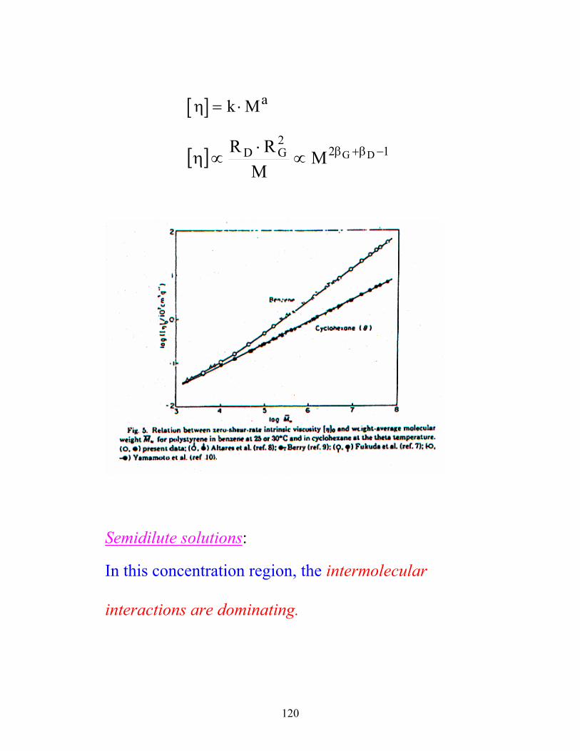
[ ]η = ⋅k Ma
[ ] 122GD DGM
MRR −β+β∝⋅
∝η
Semidilute solutions: In this concentration region, the intermolecular
interactions are dominating.
121
At a certain concentration, c*, (”overlap
concentration”) the polymer molecules starts to
overlap with each other, and a transient network is
formed.
Static experiments:
c MR
MG
G*∝ ∝ −3
1 3β
c* ∝ M-0.76 (good conditions) c* ∝ M-0.50 (θ-conditions) Dynamical experiments:
[ ]c M G D* = ∝ − −1 1 2
ηβ β
122
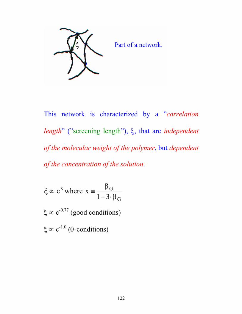
This network is characterized by a ”correlation
length” (”screening length”), ξ, that are independent
of the molecular weight of the polymer, but dependent
of the concentration of the solution.
G
Gx
31xwherec
β⋅−β
≡∝ξ
ξ ∝ c-0.77 (good conditions) ξ ∝ c-1.0 (θ-conditions)
123
Scaling laws in the semidilute region is based on the
existence of an overlap concentration, c*, where the
concentration dependence of a given parameter (Π, S,
D) is changing.
In addition to the existence of a correlation length, ξ,
that are dependent on the polymer concentration, but
independent on the molecular weight of the polymer.
Concentrated solutions
A homogenous distribution of segments in the
solution. At a concentration, c+, the chain dimensions
will be independent of the concentration and assume
their non-perturbed dimensions. (c>15 %); [ ]θ+
η=
6c .
124
Illustration of characteristic lengths and concentration
regions
Description of semidilute polymer solutions with
the aid of the "Blob" model.
125
A semidilute solution may be considered to consist of
a string of ”blobs” of the size ξ. Each ”blob” has the
molecular weight (ξG ∝ cβ/(1-3β))
β⋅−∝ξ⋅∝ξ 31
13G cc)(M
Phenomenological consideration of osmotic pressure,
diffusion and sedimentation with the aid of Scaling-
laws
Osmotic pressure:
( )Π = ⋅ ⋅ + + + ⋅⋅R TM
c A c A c22
33
”Mean field" (Flory): Π ≈ c2 (good conditions) Π ≈ c3 (θ-conditions)
126
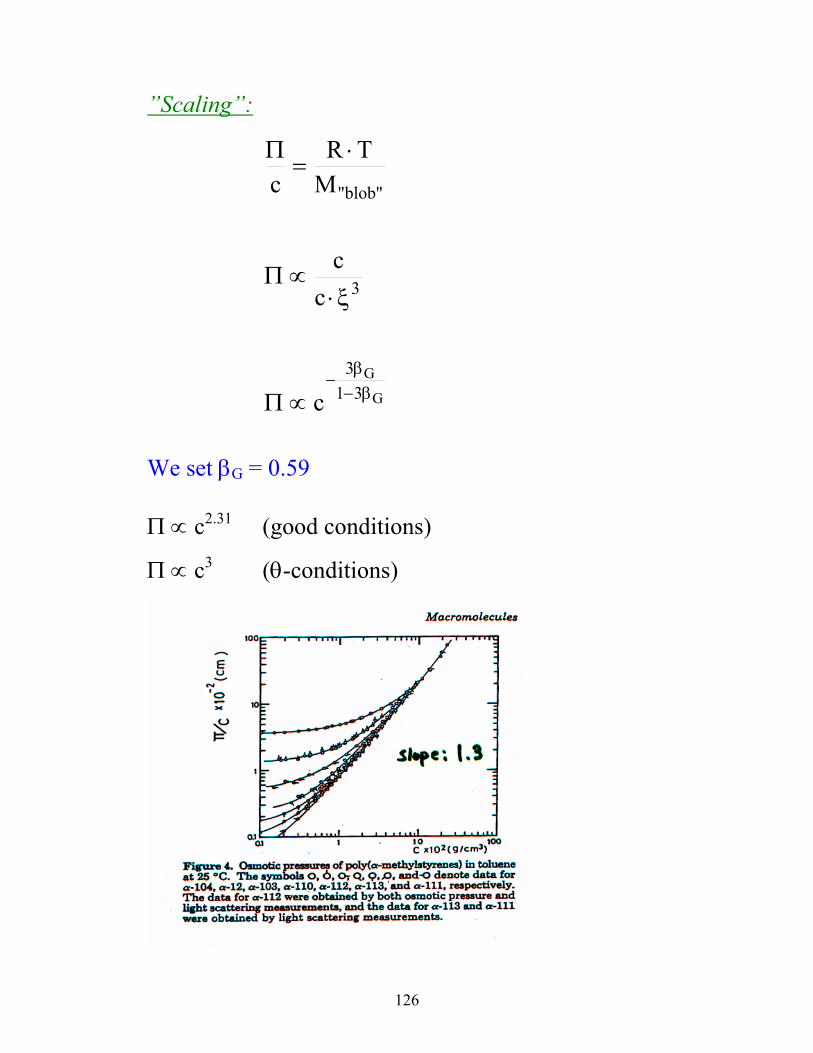
”Scaling”:
G
G31
3
3
"blob"
c
cc
MTR
c
β−β
−∝Π
ξ⋅∝Π
⋅=
Π
We set βG = 0.59
Π ∝ c2.31 (good conditions)
Π ∝ c3 (θ-conditions)
127
In order to simplify the analysis of diffusion- and
sedimentation data, we assume: M → ∞, then
βG = βD = β and ξG = ξD = ξ.
Diffusion (cooperative):
1
06TkD −ξ∝
ξ⋅η⋅π⋅
=
D c∝−− ⋅ββ1 3
D ∝ c0.77 (good conditions) D ∝ c1.0 (θ-conditions) Sedimentation (cooperative):
β−β
+∝ξ⋅∝
ξ⋅η⋅πξ⋅
∝ξ⋅η⋅π
∝⋅ρ⋅−
⋅= 3121
2
0
3
0
"blob"
A
2 cc6
c6M
fNv1MS
S c∝
−−
11 3
ββ
S ∝ c-0.53 (good conditions) S ∝ c-1.0 (θ-conditions)
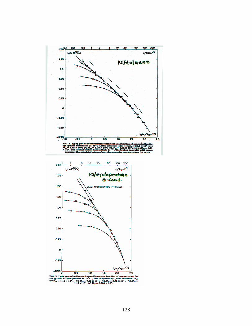
128
129
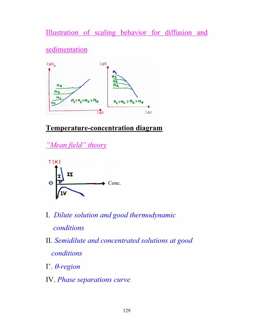
Illustration of scaling behavior for diffusion and
sedimentation
Temperature-concentration diagram
”Mean field” theory
Conc.
I. Dilute solution and good thermodynamic
conditions
II. Semidilute and concentrated solutions at good
conditions
I’. θ-region
IV. Phase separations curve
130
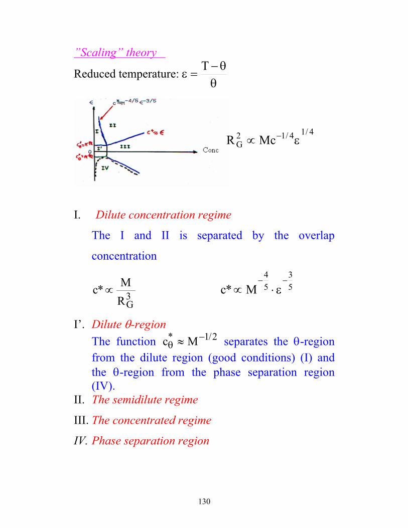
”Scaling” theory
Reduced temperature: θθ−
=εT
I. Dilute concentration regime
The I and II is separated by the overlap
concentration
c MRG
*∝ 3 53
54
M*c−−ε⋅∝
I’. Dilute θ-region The function c Mθ
* /≈ −1 2 separates the θ-region from the dilute region (good conditions) (I) and the θ-region from the phase separation region (IV).
II. The semidilute regime
III. The concentrated regime
IV. Phase separation region
4/14/12G McR ε∝ −
131
RHEOLOGY AND THE MECHANICAL
PROPERTIES OF POLYMERS
Rheology:
i) Viscous flow - irreversible deformation
ii) Rubber elasticity - reversible deformation
iii) Viscoelasticity - the deformation is reversible,
but time dependent
iv) ”Hookean” elasticity - the motion of the chain
segment is very restricted, but involves bound
stretching and bound angle deformation
Crystalline – first order transition (ice-water) Polymers Amorphous – chains that cannot be arranged in an ordered way
132
”Glass”-rubber transitions
Simple mechanical relations:
Young's-modulus:
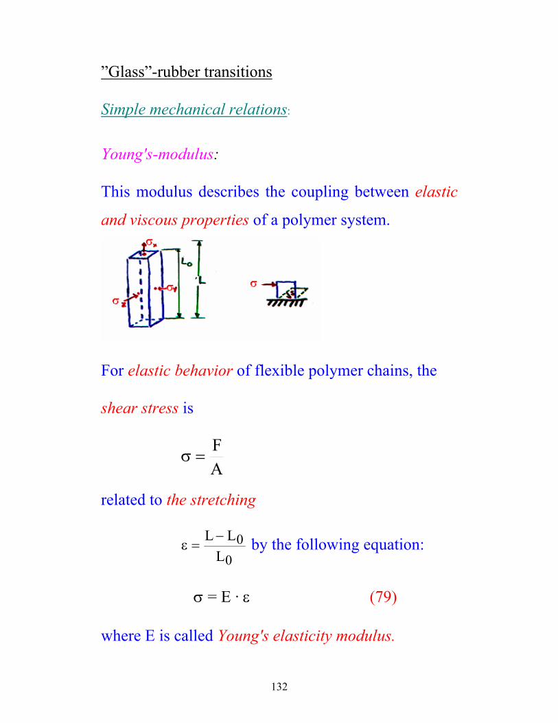
This modulus describes the coupling between elastic
and viscous properties of a polymer system.
For elastic behavior of flexible polymer chains, the
shear stress is
AF
=σ
related to the stretching
ε =−L LL
00
by the following equation:
σ = E · ε (79)
where E is called Young's elasticity modulus.
133
This modulus gives information of the stiffness of the
polymer. The higher E, the greater tendency the
polymer material has to resist stretching.
Ex.
Material E (Pa)
copper 1.2·1011
polystyrene 3·109
soft rubber 2·106 Shear modulus:
sG σ= ; s = shear deformation (shear angle)
Newton's law: The equation for an ideal liquid with viscosity η, may be written as:
dtds⋅η=σ (80)
dtds = shear deformation rate
Equ. (80) describes the viscosity for simple liquids at low flow rates.
134
Compliance and modulus
The modulus measures the stiffness or hardness for an
object, while the compliance, J, measures the
softness. The elastic compliance is defined in the
following way:
JE
=1
(81)
Storage- and loss moduli
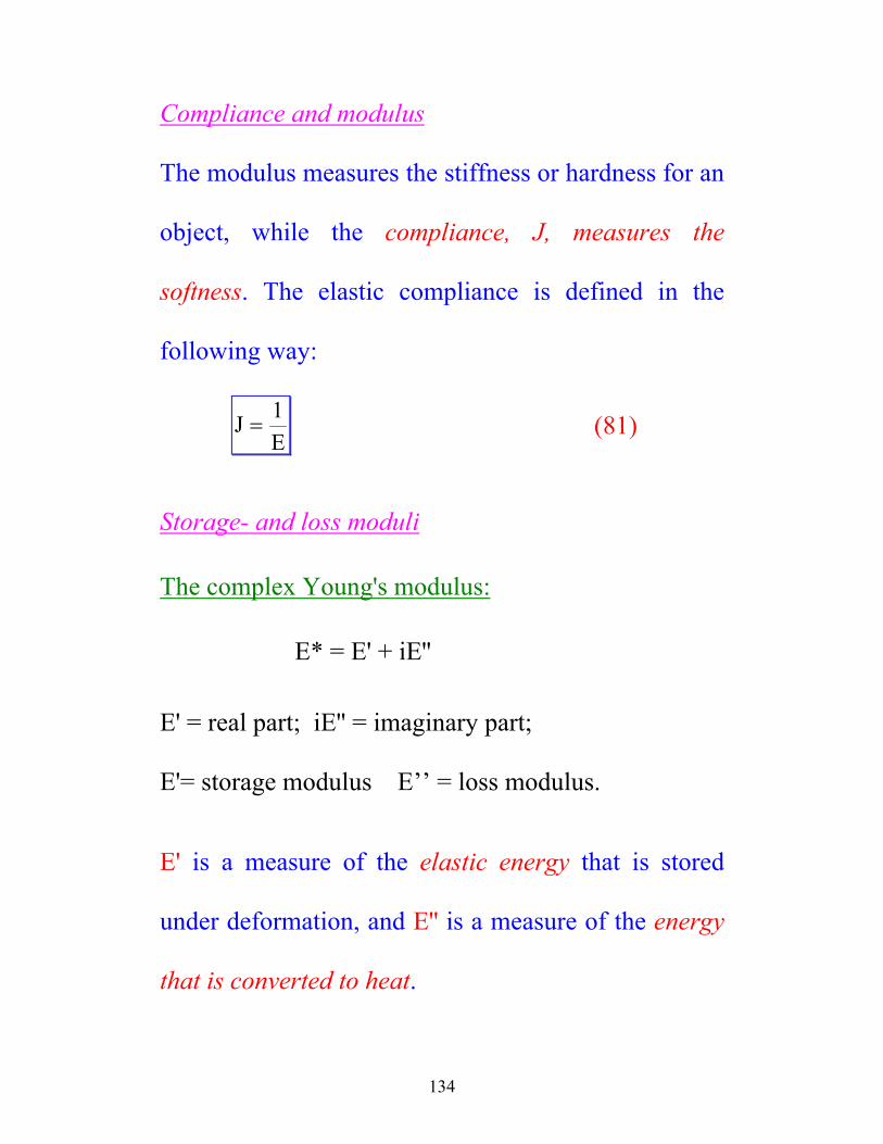
The complex Young's modulus:
E* = E' + iE'' E' = real part; iE'' = imaginary part;
E'= storage modulus E’’ = loss modulus.
E' is a measure of the elastic energy that is stored
under deformation, and E'' is a measure of the energy
that is converted to heat.
135
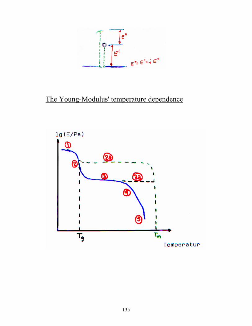
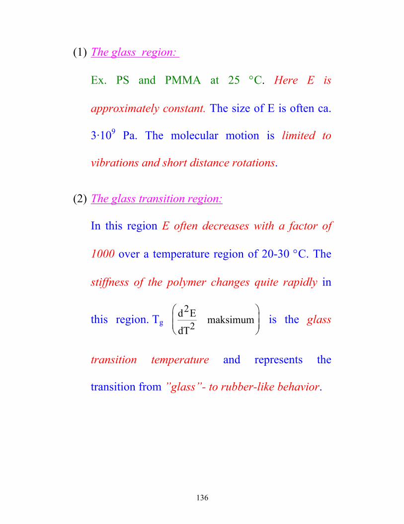
The Young-Modulus' temperature dependence
136
(1) The glass region:
Ex. PS and PMMA at 25 °C. Here E is
approximately constant. The size of E is often ca.
3·109 Pa. The molecular motion is limited to
vibrations and short distance rotations.
(2) The glass transition region:
In this region E often decreases with a factor of
1000 over a temperature region of 20-30 °C. The
stiffness of the polymer changes quite rapidly in
this region. Tg d E
dTmaksimum
2
2
is the glass
transition temperature and represents the
transition from ”glass”- to rubber-like behavior.
137
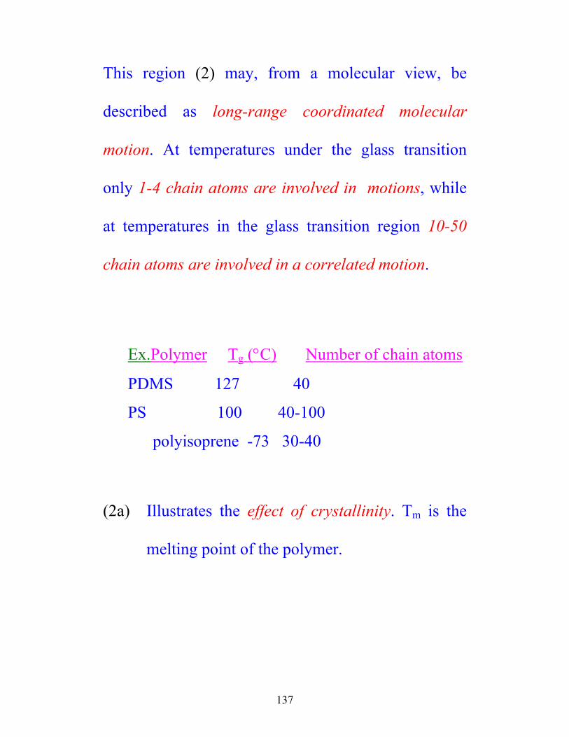
This region (2) may, from a molecular view, be
described as long-range coordinated molecular
motion. At temperatures under the glass transition
only 1-4 chain atoms are involved in motions, while
at temperatures in the glass transition region 10-50
chain atoms are involved in a correlated motion.
Ex.Polymer Tg (°C) Number of chain atoms
PDMS 127 40
PS 100 40-100
polyisoprene -73 30-40
(2a) Illustrates the effect of crystallinity. Tm is the
melting point of the polymer.
138
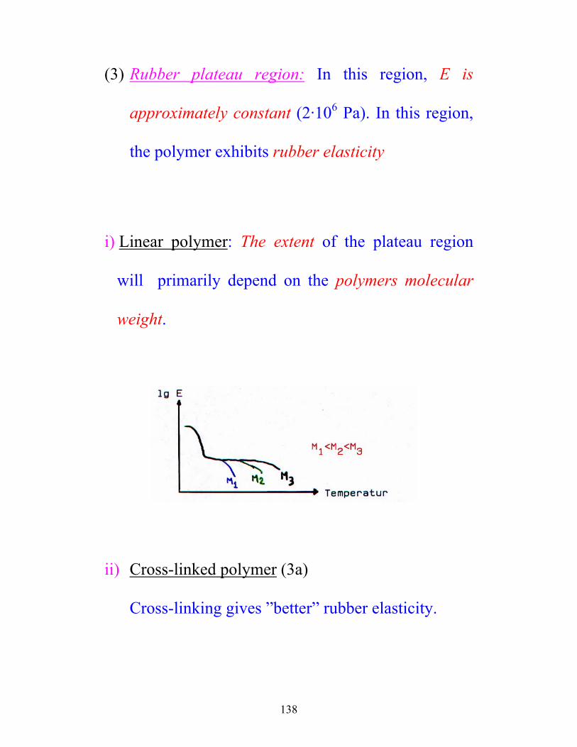
(3) Rubber plateau region: In this region, E is
approximately constant (2·106 Pa). In this region,
the polymer exhibits rubber elasticity
i) Linear polymer: The extent of the plateau region
will primarily depend on the polymers molecular
weight.
ii) Cross-linked polymer (3a)
Cross-linking gives ”better” rubber elasticity.
139
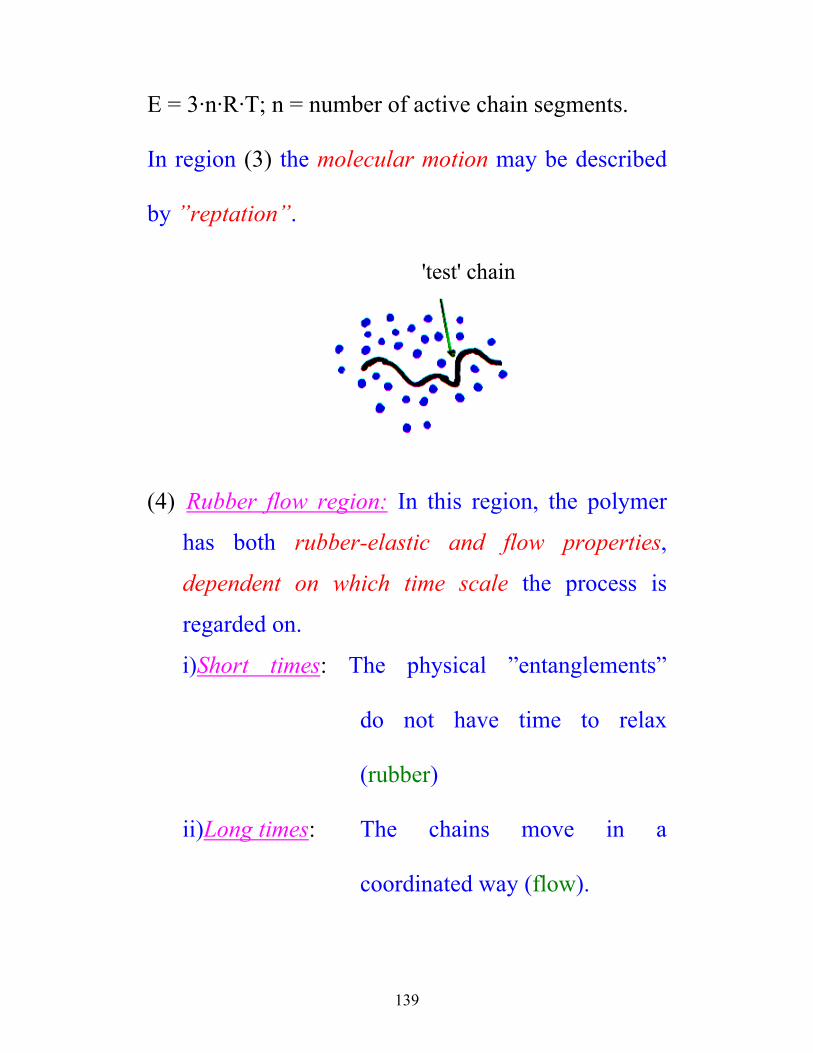
E = 3·n·R·T; n = number of active chain segments.
In region (3) the molecular motion may be described
by ”reptation”.
'test' chain
(4) Rubber flow region: In this region, the polymer
has both rubber-elastic and flow properties,
dependent on which time scale the process is
regarded on.
i)Short times: The physical ”entanglements”
do not have time to relax
(rubber)
ii)Long times: The chains move in a
coordinated way (flow).
140
(5) The liquid flow region: Here the polymer exhibits
flow properties dtds⋅η=σ at ideal conditions. This
region may also be describes by the ”reptation”
model.
Viscous flow: dtds⋅η=σ
σ = shear stress; dtds = the shear deformation rate
THE MOLECULAR WEIGHT DEPENDENCE OF
THE VISCOSITY
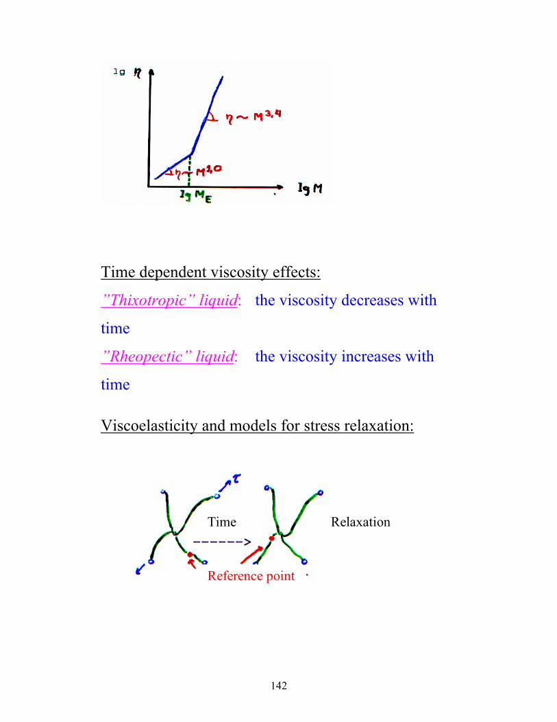
At molecular weights lower than the ”entanglement”
molecular weight (ME): η ∝ M1.0
141
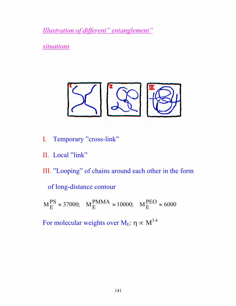
Illustration of different” entanglement”
situations
I. Temporary ”cross-link”
II. Local ”link”
III. ”Looping” of chains around each other in the form
of long-distance contour
M M MEPS
EPMMA
EPEO≈ ≈ ≈37000 10000 6000; ;
For molecular weights over ME: η ∝ M3.4
142
Time dependent viscosity effects:
”Thixotropic” liquid: the viscosity decreases with
time
”Rheopectic” liquid: the viscosity increases with
time Viscoelasticity and models for stress relaxation:
Time
Reference point
Relaxation
143
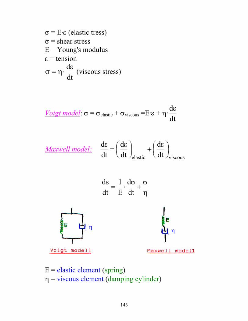
σ = E·ε (elastic tress) σ = shear stress E = Young's modulus ε = tension
dtdε⋅η=σ (viscous stress)
Voigt model: σ = σelastic + σviscous =E·ε + η·dtdε
Maxwell model: viscouselastic dt
ddtd
dtd
ε
+
ε
=ε
ησ
+σ
⋅=ε
dtd
E1
dtd
η η
E = elastic element (spring) η = viscous element (damping cylinder)
144
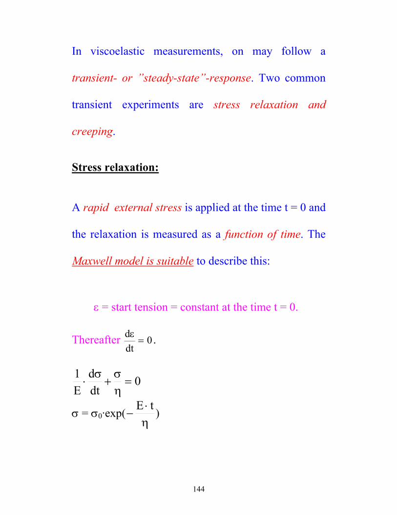
In viscoelastic measurements, on may follow a
transient- or ”steady-state”-response. Two common
transient experiments are stress relaxation and
creeping.
Stress relaxation: A rapid external stress is applied at the time t = 0 and
the relaxation is measured as a function of time. The
Maxwell model is suitable to describe this:
ε = start tension = constant at the time t = 0.
Thereafter ddtε= 0.
0dtd
E1
=ησ
+σ
⋅
σ = σ0·exp(η⋅
−tE )
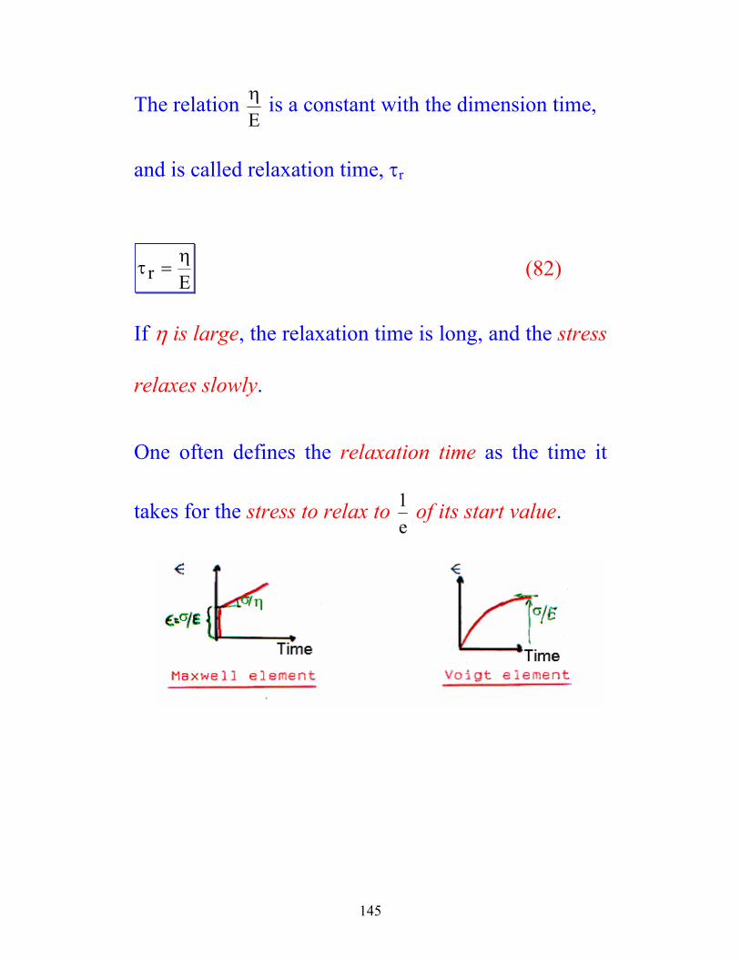
145
The relation ηE
is a constant with the dimension time,
and is called relaxation time, τr
τη
r E= (82)
If η is large, the relaxation time is long, and the stress
relaxes slowly.
One often defines the relaxation time as the time it
takes for the stress to relax to 1e
of its start value.
146
Creep: In this experiment a constant external strain is
applied at the time t = 0. The deformation is
measured as a function of time by keeping the stress
constant. To describe creep, Voigt's model is often
used: The stress is constant σ = σo.
dtdE0ε
⋅η+ε⋅=σ (83)
η⋅
−−=σε
⋅tEexp1E
0 (84)
The ratio ηE
is called the retardation time of a creep
experiment.
147
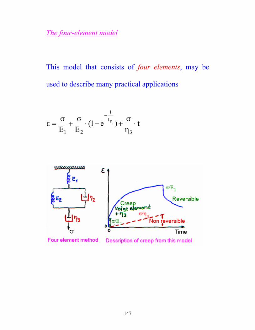
The four-element model
This model that consists of four elements, may be
used to describe many practical applications
t)e1(EE 3
tt
21⋅
ησ
+−⋅σ
+σ
=ε η−
148
RUBBER ELASTICITY The natural material rubber (C5H8)n (isoprene) The following three conditions must be fulfilled for a
material to exhibit rubber properties:
1) It has to consist of long chain molecules with
bounds that permit free rotation
2) The forces between the molecules must be weak as
in a liquid
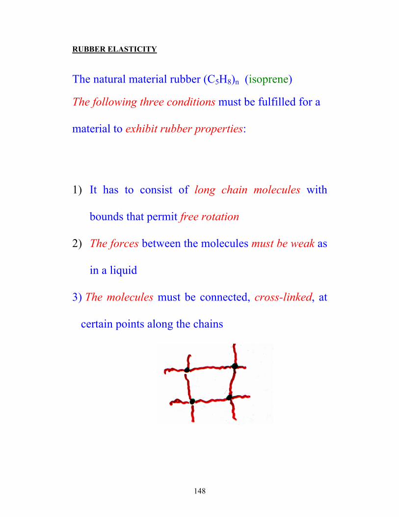
3) The molecules must be connected, cross-linked, at
certain points along the chains
149
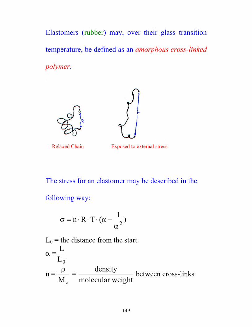
Elastomers (rubber) may, over their glass transition
temperature, be defined as an amorphous cross-linked
polymer.
Relaxed Chain Exposed to external stress
The stress for an elastomer may be described in the
following way:
)1(TRn 2α−α⋅⋅⋅=σ
L0 = the distance from the start
α =0L
L
n = cMρ =
weightmoleculardensity between cross-links
150
n represents the number of ”active” network segments
pr. unity volume.
THERMODYNAMICS FOR RUBBER
ELASTICITY
When one talks about equilibriums in systems that
changes in a reversible way (e.g. elastic deformation),
it is practical to introduce Helmholtz free energy, A,
defined by:
A = U - T·S; U = inner energy (85)
The backward-pulling force, f, which operates on the
elastomer, is dependent on the change in free energy
when the distance is changed:
151
f Al
Ul
T SlT V T V T V
=
=
− ⋅
∂∂
∂∂
∂∂, , ,
(86)
For an ideal elastomer: ∂∂Ul T V
=,
0
for most other materials (e.g. a steel rod):
T Sl T V
⋅
=∂∂ ,
0
One may show that there is a direct correlation
between the entropy and f:
−
=
∂∂
∂∂
Sl
fTT V l V, ,
(87)
152
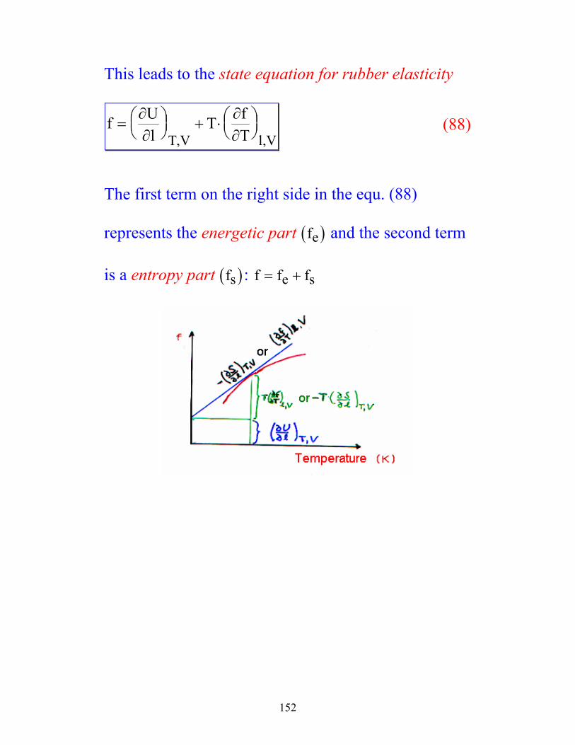
This leads to the state equation for rubber elasticity
f Ul
T fTT V l V
=
+ ⋅
∂∂
∂∂, ,
(88)
The first term on the right side in the equ. (88)
represents the energetic part ( )fe and the second term
is a entropy part ( )fs : f f fe s= +


![Supporting Information - Max Planck Society · For valine three different rotameric states can exist in solution, the trans (t), gauche+ (p), and gauche-(m)[32]. We were interested](https://img.pdfslide.us/doc/110x75/6065cf05895239668077687e/supporting-information-max-planck-society-for-valine-three-different-rotameric.jpg)