Embed Size (px)
Citation preview

Journal of Computational and Applied Mathematics 183 (2005) 29–52
www.elsevier.com/locate/cam
General explicit difference formulas for numerical differentiationJianping Li∗
National Key Laboratory of Numerical Modeling for Atmospheric Science and Geophysical Fluid Dynamics (LASG), Instituteof Atmospheric Physics, Chinese Academy of Sciences, P.O. Box 9804, Beijing 100029, China
Received 6 November 2003; received in revised form 5 December 2004
Abstract
Through introducing the generalized Vandermonde determinant, the linear algebraic system of a kind of Van-dermonde equations is solved analytically by use of the basic properties of this determinant, and then we presentgeneral explicit finite difference formulas with arbitrary order accuracy for approximating first and higher deriva-tives, which are applicable to unequally or equally spaced data. Comparing with other finite difference formulas, thenew explicit difference formulas have some important advantages. Basic computer algorithms for the new formulasare given, and numerical results show that the new explicit difference formulas are quite effective for estimatingfirst and higher derivatives of equally and unequally spaced data.© 2005 Elsevier B.V. All rights reserved.
MSC:65D25; 15A06; 65L12
Keywords:Numerical differentiation; Explicit finite difference formula; Generalized Vandermonde determinant; Taylor series;Higher derivatives
1. Introduction
Numerical differentiation is not only an elementary issue in numerical analysis[2,7,28], but also avery useful tool in applied sciences[3,26]. In practice, numerical approximations to derivatives are usedmainly in two ways. First, we want to compute the derivatives of a function at specified points within itsdomain. The function is given to us either in the form of a discrete set of argument and function values,or in a continuous analytical form. Second, we use the numerical differentiation formulae in deriving
∗ Tel.: +86 10 6203 5479; fax: +86 10 6204 3526.E-mail address:[email protected](J. Li).
0377-0427/$ - see front matter © 2005 Elsevier B.V. All rights reserved.doi:10.1016/j.cam.2004.12.026
30 J. Li / Journal of Computational and Applied Mathematics 183 (2005) 29–52
numerical methods for solving ordinary differential equations (ODEs) and partial differential equations(PDEs).
A number of different techniques have been developed to construct useful difference formulas for nu-merical derivatives. Most approaches of them fall into five categories: finite difference type[2–4,7,17–22,25,26,28], polynomial interpolation type[2,3,7–9,11,27,28], operator type[7,33], lozenge diagrams[10],and undetermined coefficients[10,14]. Other numerical differentiation methods, which do not aim at de-veloping difference formulas of derivatives but evaluating numerical derivatives by use of data or givenanalytical forms of functions, include: Richardson extrapolation[2,3,7,16,25,28], spline numerical dif-ferentiation[36,37], regularization method[1,6,23,35], and automatic differentiation (AD)[5,12,13,30].
The AD is an accurate differentiation technique based on the mechanical application of the chain ruleto obtain the derivatives of a function expressed by a computer program, but it cannot be applied to thecases in which analytical expressions of functions are unknown. However, it is very familiar in practicethat the derivatives of a function whose values are only obtained empirically at a discrete set of pointsneed to be evaluated. The regularization method on numerical differentiation is effective and stable forestimating the first derivative of a function with non-exact data. This kind of method is divided mainlyinto three sorts: parameter regularization[31,32], mollification regularization[15,29,35]and variationalregularization[24,34]. However, some of the regularization methods strongly depend on a regularizationparameter whose optimal value choice is a nontrivial task. Some of the methods are limited to cases inwhich the spectrum of the data shows a clear division between the signal of the correct function and thenoise, and some of them depend on solving a boundary value problem of second order differential equationwhose numerical solutions themselves involve difference methods. It is difficult not only to improve themethods mentioned above so that they are approximations of higher order to derivatives, but also to usethem directly to find higher derivatives. The dependence on evenly data is also another disadvantage. Analternative approach for evaluating derivatives is to use the Richardson extrapolation[2,3,7,16,25,28].The technique, however, is actually equivalent to fitting a higher-order polynomial through the data andthen computing the derivatives by centered differences[3]. Moreover, for the Richardson extrapolation,the data have to be evenly spaced and generated for successively halved intervals. Evidently, it is notapplicable to the case of non-uniform data. A common characteristic of these methods stated above isthat they cannot generally provide explicit difference formulas of derivatives for designing differenceschemes of both ODEs and PDEs.
Numerical differentiation formulas based on interpolating polynomials (e.g., Lagrangian, Newton,Chebyshev, Hermite, Guass, Bessel, Sterling interpolating polynomials, and etc.) may be found in manyliteratures[2,3,7–9,11,27,28]. The advantages of the methods are that they do not require that the databe equispaced, and some specific difference formulas deduced from the methods can be used to estimatethe derivative anywhere within the range prescribed by the known points. Unfortunately, the methods aregenerally implicit. Take Lagrange interpolating polynomial as an example, by using the polynomial maygenerate general derivate approximation formulas as follows:
f (m)(xi)=n∑k=0
L(m)k (xi)f (xk)+ R(xi), i = 0,1, . . . , n, (1.1)
whereLk(x) denotes thekth Lagrange polynomial for the functionf atx0, x1, . . . , xn in some intervalI ,f ∈ Cn+1(I ), andR(x) is the remainder term Eq. (1.1) is called an(n+1)-point formula to approximatef (m)(xi). In general, it cannot be directly used to calculate the derivatives due to its dependence onL
(m)k (x)

J. Li / Journal of Computational and Applied Mathematics 183 (2005) 29–52 31
which is a very complex polynomial and depends on lower derivatives. Besides, it is also complicatedto derive higher-order finite difference formulas by means of the method. By using operators[7,33] andby using lozenge diagrams[10] are other two useful and simple approaches to find numerical differen-tiation formulas. In fact, all the formulas constructed by interpolating polynomials can be generated byapplying operators or lozenge diagrams. However, all of these formulas use difference tables constructedfrom sampling data and recursive procedures by expanding the higher differences step-by-step to lowerdifferences.
Another alternative way for developing difference formulas is the method of undetermined coefficients,which solvesn linear algebraic equations derived from certain polynomial or Taylor expansions, byimposingn necessary conditions on it[10,14]. The calculation complexity of the determination of thecoefficients by solvingn linear equations is drastically increased while the order of the approximationincreases. Moreover, a new system of equations needs to be re-solved to obtain all coefficients if the orderof the approximation is changed. Therefore, the method is limited to lower orders due to its complexityin calculation. However, direct use of the method will become wide if the general algebraic solutions ofthe linear equations on the coefficients can be theoretically found.
Based on Taylor series, recently, Khan et al.[17–21]have presented the explicit forward, backwardand central difference formulas of finite difference approximations with arbitrary orders for first deriva-tive, and the central difference approximations for higher derivates. In essential, it can be found fromthe mathematical proofs of their explicit formulas for the coefficients of finite difference approximationsof first derivatives[22] that the explicit formulas were original from the undetermined coefficients bysolving a special kind of linear equations. Most advantages of the explicit difference formulas are theirconvenience in calculations for numerical approximations of arbitrary order to derivatives and their directuse for solution of ODEs and PDEs. The applicability of these explicit formulas, however, appears tobe limited to case in which the data had to be equispaced. In contrast, data from experiments or fieldsstudies are often collected at unequal intervals, and such information cannot be analyzed with the explicitformulas mentioned above to this point. Thus, explicit techniques to handle nonequispaced data needto be developed. Besides, the coefficients of explicit central difference formulas for higher derivativeswith evenly spaced data were only given in[17,21] based on numerical results, but any mathematicalproof was not shown. Obviously, it is also worth studying for explicit forward and backward differenceformulas for higher derivatives except that the explicit central difference formulas for higher derivativesin [17,21] should be proved. Moreover, the explicit forward, backward and central difference formulasdo not give the whole circumstance. For example, if there are an eight given values of a functionf atpointsx0<x1< · · ·<x7, and one wants an 8-point difference formula to approximate first derivatives off atx1, then the explicit 8-point forward, backward and central difference formulas given in[17–21]arenot available to this question since information aboutf outside the interval is not available. Therefore,the explicit approximation formulas to derivatives near the ends of an interval also need to be developed.In this paper, we study these questions, and present general explicit finite difference formulas for numer-ical differentiation at unequally or equally spaced gird-points that we believe avoids those limitationsmentioned above.
In Section 2, the main explicit difference formulas of arbitrary order for first and higher numericalderivatives are given for unequally or equally spaced data. In Section 3, annth generalized Vandermondedeterminant is introduced, its basic properties are discussed and other some necessary lemmas are given.Moreover, the linear algebraic system of a kind of Vandermonde equations is solved analytically. Basedon the lemmas and Taylor series the proofs of the main results described in Section 2 are then shown
32 J. Li / Journal of Computational and Applied Mathematics 183 (2005) 29–52
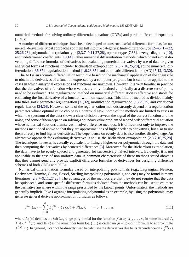
in Section 4. In Section 5, the new explicit formulas are compared with other finite difference formulas.Section 6 shows a discussion of numerical results with details of our implementation, combining withbasic computer algorithms of the new formulas of equally and unequally spaced data for differenceapproximations of any order to first and higher derivatives of a function whose values are known only ata discrete set of points. Section 7 is devoted to a brief conclusion.
2. Main results
Suppose thatx1, x2, . . . , xn aren distinct real numbers, let
a(0)n = a0(x1, x2, . . . , xn)= x1x2 · · · xn,a(1)n = a1(x1, x2, . . . , xn)= x1x2 · · · xn−1 + x1x2 · · · xn−2xn + · · · + x1x3 · · · xn + x2x3 · · · xn,a(2)n = a2(x1, x2, . . . , xn)= x1x2 · · · xn−2 + · · · + x3x4 · · · xn,
· · ·a(n−2)n = an−2(x1, x2, . . . , xn)= x1x2 + x1x3 + · · · + xn−1xn,
a(n−1)n = an−1(x1, x2, . . . , xn)= x1 + x2 + · · · + xn,a(n)n = an(x1, x2, . . . , xn)= 1.
(2.1)
And let�ij = xj − xi , writing the first divided difference of the functionf with respect toxi andxj as
D(xi, xj )= f (xj )− f (xi)xj − xi = f (xj )− f (xi)
�ij, (2.2)
wherei �= j .Theorem 2.1. If x0<x1< · · ·<xn are(n+1) distinct numbers in the interval[a, b] andf is a functionwhose values are given at these numbers andf ∈ Cn+1[a, b], then for any onexi (i = 0,1, . . . , n) onecan use the linear combination ofD(xi, xj ) (j = 0,1, . . . , n andj �= i) to construct an(n + 1)-pointformula to approximatef ′(xi), i.e.
f ′(xi)=n∑
j=0,j �=icn,i,jD(xi, xj )+ Rn(xi), (2.3)
where the coefficients
c1,0,1 = 1 and c1,1,0 = 1, for n= 1, (2.4)
cn,i,j =n∏
k=0,k �=i,k �=j
(xk − xi)(xk − xj ) , j �= i, n>1, and i, j = 0,1, . . . , n, (2.5)

J. Li / Journal of Computational and Applied Mathematics 183 (2005) 29–52 33
and the remainder term
R1(x0)= f′′(�0)
2(x0 − x1) and R1(x1)= f
′′(�1)
2(x1 − x0), for n= 1, (2.6)
Rn(xi)= 1
(n+ 1)!n∏
k=0,k �=i(xi − xk)
n∑j=0,j �=i
f (n+1)(�j )(xi − xj )n−1∏nk=0,k �=i,k �=j (xk − xj ) , for n>1, (2.7)
where�j depends onxj andxi .
Remark 2.1. The sum of the weighing coefficientscn,i,j for any reference pointxi is one, i.e.
n∑j=0,j �=i
cn,i,j = 1, i = 0,1, . . . , n, and n�1. (2.8)
This property of the differentiation approximation (2.3) guarantees that the first derivative of a linearfunction is a constant. In fact, forn>1 and any real numberx one has a more general formula as follows:
n∑j=1
n∏k=1,k �=j
(xk − x)(xk − xj ) = 1. (2.9)
Remark 2.2. For n>1 the coefficients off (n+1)(�j ) (j = 0,1, . . . , n) in (2.7) satisfy the followingrelation:
n∑j=0,j �=i
(xi − xj )n−1∏nk=0,k �=i,k �=j (xk − xj ) = 1, i = 0,1, . . . , n. (2.10)
Forn>1 and any real numberx, in fact, one can write
n∑j=1
n∏k=1,k �=j
(x − xj )(xk − xj ) = 1. (2.11)
Corollary 2.1. If x0, x1, . . . , xn are(n+1) distinct numbers in the interval[a, b], they are equally spacednotes,i.e.,
xi = x0 + ih (i = 0,1, . . . , n) for someh �= 0
and f is a function whose values are given at these notes andf ∈ Cn+1[a, b], then for any onexi (i = 0,1, . . . , n) one can use the linear combination off (xj ) (j = 0,1, . . . , n) to construct an(n+ 1)-point formula to approximatef ′(xi), i.e.
f ′(xi)= 1
h
n∑j=0
dn+1,i,j f (xj )+On,i(hn), (2.12)
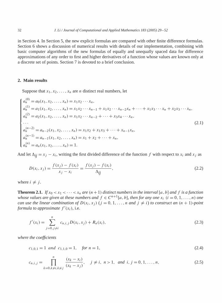
34 J. Li / Journal of Computational and Applied Mathematics 183 (2005) 29–52
where the coefficients
dn+1,i,j = (−1)i−j+1
j − ii!(n− i)!j !(n− j)! , i, j = 0,1, . . . , n and j �= i, (2.13)
dn+1,i,i = −n∑
j=0,j �=idn+1,i,j (2.14)
and the remainder term
On,i(hn)= (−1)n−i i!(n− i)!hn
(n+ 1)!n∑
j=0,j �=i
f (n+1)(�j )(i − j)n(−1)j j !(n− j)! , (2.15)
where�j depends onxj andxi .
Remark 2.3. It can been seen from (2.13) and (2.14) that the sum of the weighing coefficientsdn+1,i,jfor any giveni (i=0,1, . . . , n),
∑nj=0 dn+1,i,j =0, to ensure that the slope of a constant function is zero.
Moreover,∑nj=0(j − i)dn+1,i,j = 1 guarantees that the first derivative of a linear function is a constant.
Remark 2.4. The coefficientsdn+1,i,j are anti-symmetric, i.e.
dn+1,i,j = −dn+1,n−i,n−j , (2.16)
wheren�1, j = 0,1, . . . , n, i = 0,1, . . . , [n/2], here the symbol[x] denotes the greatest integer notgreater thanx. Especially, whenn=2l, wherel is a natural number,d2l+1,l,l=0,d2l+1,l,j =−d2l+1,l,l−j ,j = 0,1, . . . , l − 1. In this case, one can use the function values atn points (n is an even number) toconstruct ann order numerical differentiation of the first derivativef ′(xl) at the middle pointxl . Asknown, at this time the difference approximation is called the central differentiation.
Remark 2.5. In practice, to reduce computational burden, for large numbern, one can use the followingrecursive procedure to calculate the coefficientsdn+1,i,j :
A0 = 0!n!, (2.17)
Ai = Ai−1i
(n− i + 1), i = 1, . . . , n, (2.18)
dn+1,i,j = (−1)i−j+1
j − iAi
Aj, i = 0,1, . . . , [n/2], j = 0,1, . . . , n, and j �= i (2.19)
anddn+1,i,i is calculated by (2.14), and the other coefficientsdn+1,i,j (i=[n/2]+1, . . . , n, j=0,1, . . . , n,j �= i) can be obtained easily by use of the formula (2.16).
Remark 2.6. Forn>1 and any giveni (i=0,1, . . . , n), the coefficients off (n+1)(�j ) (j=0,1, . . . , n)in the remainder term (2.15) satisfy
n∑j=0,j �=i
(i − j)n(−1)j j !(n− j)! = 1. (2.20)

J. Li / Journal of Computational and Applied Mathematics 183 (2005) 29–52 35
Theorem 2.2. If x0, x1, . . . , xn are (n + 1) distinct numbers in the interval[a, b] andf is a functionwhose values are given at these numbers andf ∈ Cn+1[a, b], then for any onexi (i = 0,1, . . . , n) onecan use the linear combination ofD(xi, xj ) (j = 0,1, . . . , n andj �= i) to construct an(n + 1)-pointformula to approximate themth derivativef (m)(xi) wherem�n, i.e.
f (m)(xi)=n∑
j=0,j �=ic(m)n,i,jD(xi, xj )+ R(m)n (xi), (2.21)
where the coefficients
c(1)1,0,1 = 1 and c(1)1,1,0 = 1, for n= 1, (2.22)
c(m)n,i,j = (−1)m−1m!a(m−1)
n−1,i,j∏nk=0,k �=i,k �=j (xk − xj ) , for n>1, j �= i and i, j = 0,1, . . . , n, (2.23)
wherea(m−1)n−1,i,j = am−1(�i0, . . . ,�ik, . . . ,�in) (k = 0,1, . . . , n andk �= i, j ). The remainder term
R(1)1 (x0)= f
′′(�0)
2(x0 − x1) and R
(1)1 (x1)= f
′′(�1)
2(x1 − x0), for n= 1, (2.24)
R(m)n (xi)= (−1)n−mm!(n+ 1)!
n∑j=0,j �=i
f (n+1)(�j )a(m−1)n−1,i,j (xi − xj )n∏n
k=0,k �=i,k �=j (xk − xj ) , for n>1, (2.25)
where�j depends onxj andxi .
Remark 2.7. It may be shown that, withm�2, the sum of the weighing coefficientscn,i,j for anyreference pointxi is zero, i.e.
n∑j=0,j �=i
c(m)n,i,j = 0, 2�m�n, i = 0,1, . . . , n. (2.26)
This basic characteristic of the differentiation formula (2.12) guarantees that for anym>1 themthderivative of a linear function is always zero.
Remark2.8. Generally, the following formula can be given for parts of the coefficients off (n+1)(�j ) (j=0,1, . . . , n) in (2.25)
n∑j=0,j �=i
(xi − xj )Ka(L)n−1,i,j∏nk=0,k �=i,k �=j (xk − xj ) =
{1, for K = L,0, for K �= L, (2.27)
where 0�K�n− 1, 0�L�n− 1, i = 0,1, . . . , n.
Corollary 2.2. If x0, x1, . . . , xn are(n+1) distinct numbers in the interval[a, b], they are equally spacednotes, i.e.,
xi = x0 + ih (i = 0,1, . . . , n) for someh �= 0
36 J. Li / Journal of Computational and Applied Mathematics 183 (2005) 29–52
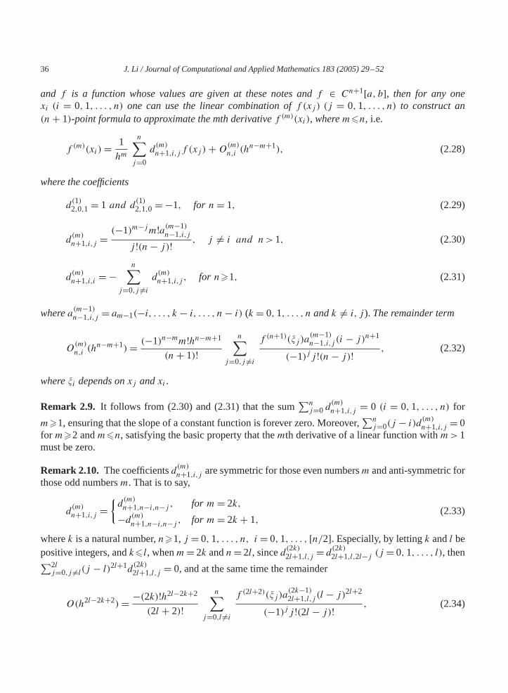
and f is a function whose values are given at these notes andf ∈ Cn+1[a, b], then for any onexi (i = 0,1, . . . , n) one can use the linear combination off (xj ) (j = 0,1, . . . , n) to construct an(n+ 1)-point formula to approximate the mth derivativef (m)(xi), wherem�n, i.e.
f (m)(xi)= 1
hm
n∑j=0
d(m)n+1,i,j f (xj )+O(m)n,i (hn−m+1), (2.28)
where the coefficients
d(1)2,0,1 = 1 and d(1)2,1,0 = −1, for n= 1, (2.29)
d(m)n+1,i,j = (−1)m−jm!a(m−1)
n−1,i,j
j !(n− j)! , j �= i and n>1, (2.30)
d(m)n+1,i,i = −
n∑j=0,j �=i
d(m)n+1,i,j , for n�1, (2.31)
wherea(m−1)n−1,i,j = am−1(−i, . . . , k − i, . . . , n− i) (k = 0,1, . . . , n andk �= i, j ). The remainder term
O(m)n,i (h
n−m+1)= (−1)n−mm!hn−m+1
(n+ 1)!n∑
j=0,j �=i
f (n+1)(�j )a(m−1)n−1,i,j (i − j)n+1
(−1)j j !(n− j)! , (2.32)
where�i depends onxj andxi .
Remark 2.9. It follows from (2.30) and (2.31) that the sum∑nj=0 d
(m)n+1,i,j = 0 (i = 0,1, . . . , n) for
m�1, ensuring that the slope of a constant function is forever zero. Moreover,∑nj=0(j − i)d(m)n+1,i,j = 0
for m�2 andm�n, satisfying the basic property that themth derivative of a linear function withm>1must be zero.
Remark 2.10. The coefficientsd(m)n+1,i,j are symmetric for those even numbersm and anti-symmetric forthose odd numbersm. That is to say,
d(m)n+1,i,j =
{d(m)n+1,n−i,n−j , for m= 2k,
−d(m)n+1,n−i,n−j , for m= 2k + 1,(2.33)
wherek is a natural number,n�1, j = 0,1, . . . , n, i = 0,1, . . . , [n/2]. Especially, by lettingk andl bepositive integers, andk� l, whenm= 2k andn= 2l, sinced(2k)2l+1,l,j = d(2k)2l+1,l,2l−j (j = 0,1, . . . , l), then∑2lj=0,j �=l(j − l)2l+1d
(2k)2l+1,l,j = 0, and at the same time the remainder
O(h2l−2k+2)= −(2k)!h2l−2k+2
(2l + 2)!n∑
j=0,l �=i
f (2l+2)(�j )a(2k−1)2l+1,l,j (l − j)2l+2
(−1)j j !(2l − j)! , (2.34)

J. Li / Journal of Computational and Applied Mathematics 183 (2005) 29–52 37
where�i depends onxj andxi . This suggests that in this case the order of central numerical differentiationof the even order derivativef (m)(x) is one more than that of non-central numerical differentiation. Ifm= 2k andn= 2l + 1, one hasa(2k−1)
2l+1,l,2l+1 = a(2k−1)2l+1,l+1,0 = 0, d(2k)2l+2,l,2l+2 = d(2k)2l+2,l+1,0 = 0. As a result,
d(2k)2l+2,l,j = d(2k)2l+2,l+1,j+1 = d(2k)2l+1,l,j , j = 0,1, . . . ,2l + 1,
d(2k)2l+2,l,j = d(2k)2l+2,l,2l−j , j = 0,1, . . . , l − 1,
d(2k)2l+2,l+1,j = d(2k)2l+2,l+1,2l+2−j , j = 1, . . . , l.
Form= 2k + 1 andn= 2l, it follows from (2.34) that
d(2k+1)2l+1,l,l = 0.
Hence, we may use the function values atn points (n is an even number) to construct a numericaldifferentiation ofn order for the odd order derivativef (m)(x) at the centered pointxl .
3. Some lemmas
As known, annth Vandermonde determinantVn is defined as
Vn = V (x1, x2, . . . , xn)=
∣∣∣∣∣∣∣∣∣
1 1 · · · 1x1 x2 · · · xnx2
1 x22 · · · x2
n· · · · · · · · · · · ·xn−1
1 xn−12 · · · xn−1
n
∣∣∣∣∣∣∣∣∣. (3.1)
Introducing thenth generalized Vandermonde determinantV(i)n as follows, fori = 0,
V (0)n = V (0)(x1, x2, . . . , xn)=
∣∣∣∣∣∣∣∣∣
x1 x2 · · · xnx2
1 x22 · · · x2
n
x31 x3
2 · · · x3n· · · · · · · · · · · ·
xn1 xn2 · · · xnn
∣∣∣∣∣∣∣∣∣, (3.2)
for i = 1, . . . , n− 1,
V (i)n = V (i)(x1, x2, . . . , xn)=
∣∣∣∣∣∣∣∣∣∣∣∣∣
1 1 · · · 1x1 x2 · · · xn· · · · · · · · · · · ·xi−1
1 xi−12 · · · xi−1
n
xi+11 xi+1
2 · · · xi+1n· · · · · · · · · · · ·
xn1 xn2 · · · xnn
∣∣∣∣∣∣∣∣∣∣∣∣∣(3.3)
and fori = n,V (n)n = V (n)(x1, x2, . . . , xn)= V (x1, x2, . . . , xn)= Vn. (3.4)
38 J. Li / Journal of Computational and Applied Mathematics 183 (2005) 29–52
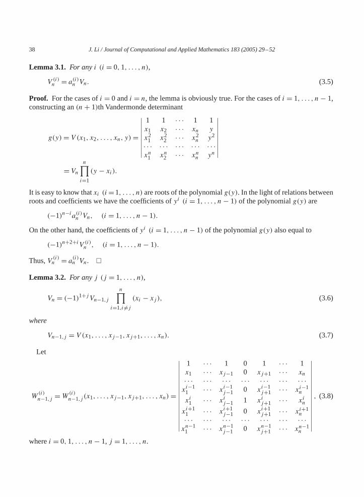
Lemma 3.1. For anyi (i = 0,1, . . . , n),
V (i)n = a(i)n Vn. (3.5)
Proof. For the cases ofi = 0 andi = n, the lemma is obviously true. For the cases ofi = 1, . . . , n− 1,constructing an(n+ 1)th Vandermonde determinant
g(y)= V (x1, x2, . . . , xn, y)=
∣∣∣∣∣∣∣∣∣
1 1 · · · 1 1x1 x2 · · · xn y
x21 x2
2 · · · x2n y2
· · · · · · · · · · · · · · ·xn1 xn2 · · · xnn yn
∣∣∣∣∣∣∣∣∣=Vn
n∏i=1
(y − xi).
It is easy to know thatxi (i=1, . . . , n) are roots of the polynomialg(y). In the light of relations betweenroots and coefficients we have the coefficients ofyi (i = 1, . . . , n− 1) of the polynomialg(y) are
(−1)n−ia(i)n Vn, (i = 1, . . . , n− 1).
On the other hand, the coefficients ofyi (i = 1, . . . , n− 1) of the polynomialg(y) also equal to
(−1)n+2+iV (i)n , (i = 1, . . . , n− 1).
Thus,V (i)n = a(i)n Vn. �
Lemma 3.2. For anyj (j = 1, . . . , n),
Vn = (−1)1+jVn−1,j
n∏i=1,i �=j
(xi − xj ), (3.6)
where
Vn−1,j = V (x1, . . . , xj−1, xj+1, . . . , xn). (3.7)
Let
W(i)n−1,j =W(i)n−1,j (x1, . . . , xj−1, xj+1, . . . , xn)=
∣∣∣∣∣∣∣∣∣∣∣∣∣∣∣∣
1 · · · 1 0 1 · · · 1x1 · · · xj−1 0 xj+1 · · · xn· · · · · · · · · · · · · · · · · · · · ·xi−1
1 · · · xi−1j−1 0 xi−1
j+1 · · · xi−1n
xi1 · · · xij−1 1 xij+1 · · · xin
xi+11 · · · xi+1
j−1 0 xi+1j+1 · · · xi+1
n· · · · · · · · · · · · · · · · · · · · ·xn−1
1 · · · xn−1j−1 0 xn−1
j+1 · · · xn−1n
∣∣∣∣∣∣∣∣∣∣∣∣∣∣∣∣
, (3.8)
wherei = 0,1, . . . , n− 1, j = 1, . . . , n.

J. Li / Journal of Computational and Applied Mathematics 183 (2005) 29–52 39
It follows from Lemma 3.1 that
Lemma 3.3. For anyi = 0,1, . . . , n− 1 andj = 1, . . . , n,
W(i)n−1,j = (−1)i+1+jV (i)n−1,j = (−1)i+1+j a(i)n−1,jVn−1,j , (3.9)
where
V(i)n−1,j = V (i)(x1, . . . , xj−1, xj+1, . . . , xn), (3.10)
a(i)n−1,j = ai(x1, . . . , xj−1, xj+1, . . . , xn) (3.11)
andVn−1,j is given by(3.7).
Lemma 3.4. For anyi (i = 0,1, . . . , n− 1),
n∑j=1
xijW(k)n−1,j =
{Vn, for i = k,0, for i �= k (3.12)
and for anyj (j = 1, . . . , n),
n−1∑i=0
xijW(i)n−1,k =
{Vn, for j = k,0, for j �= k. (3.13)
Remark 3.1. Remarks 2.1, 2.2, 2.7 and 2.8 can be derived from Lemma 3.4.
Theorem 3.1. The linear algebraic system of equations
VC =Gi, (3.14)
where
V =
1 1 · · · 1x1 x2 · · · xnx2
1 x22 · · · x2
n· · · · · · · · · · · ·xn−1
1 xn−12 · · · xn−1
n
, (3.15)
C = (c1, c2, . . . , cn)T, (3.16)
Gi = (0, . . . ,0,︸ ︷︷ ︸i−1
g,0, . . . ,0)T, (3.17)
(i = 1, . . . , n), then the solution of the system is
cj = (−1)i−1ga(i−1)n−1,j∏n
k=1,k �=j (xk − xj ) , for j = 1, . . . , n, (3.18)
wherea(i−1)n−1,j is given by(3.11).
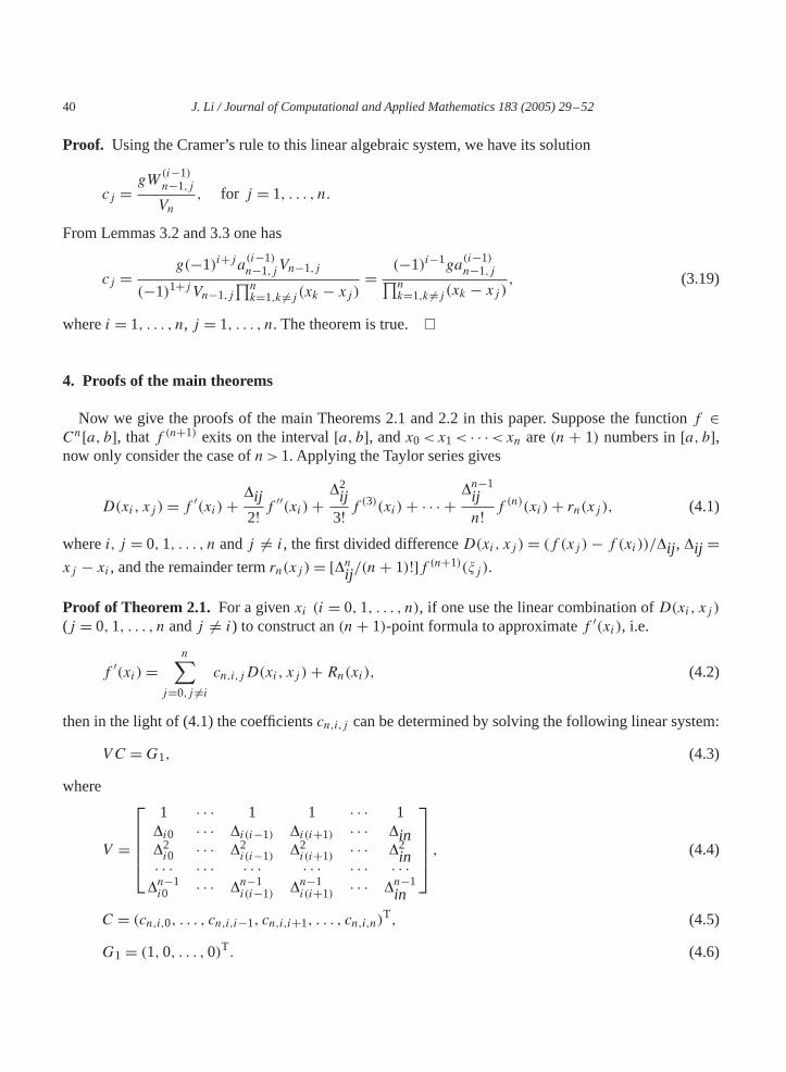
40 J. Li / Journal of Computational and Applied Mathematics 183 (2005) 29–52
Proof. Using the Cramer’s rule to this linear algebraic system, we have its solution
cj = gW(i−1)n−1,j
Vn, for j = 1, . . . , n.
From Lemmas 3.2 and 3.3 one has
cj = g(−1)i+j a(i−1)n−1,jVn−1,j
(−1)1+jVn−1,j∏nk=1,k �=j (xk − xj )
= (−1)i−1ga(i−1)n−1,j∏n
k=1,k �=j (xk − xj ) , (3.19)
wherei = 1, . . . , n, j = 1, . . . , n. The theorem is true. �
4. Proofs of the main theorems
Now we give the proofs of the main Theorems 2.1 and 2.2 in this paper. Suppose the functionf ∈Cn[a, b], thatf (n+1) exits on the interval[a, b], andx0<x1< · · ·<xn are(n + 1) numbers in[a, b],now only consider the case ofn>1. Applying the Taylor series gives
D(xi, xj )= f ′(xi)+�ij2! f
′′(xi)+�2
ij3! f
(3)(xi)+ · · · +�n−1
ijn! f
(n)(xi)+ rn(xj ), (4.1)
wherei, j = 0,1, . . . , n andj �= i, the first divided differenceD(xi, xj )= (f (xj )− f (xi))/�ij , �ij =xj − xi , and the remainder termrn(xj )= [�nij /(n+ 1)!]f (n+1)(�j ).
Proof of Theorem 2.1. For a givenxi (i = 0,1, . . . , n), if one use the linear combination ofD(xi, xj )(j = 0,1, . . . , n andj �= i) to construct an(n+ 1)-point formula to approximatef ′(xi), i.e.
f ′(xi)=n∑
j=0,j �=icn,i,jD(xi, xj )+ Rn(xi), (4.2)
then in the light of (4.1) the coefficientscn,i,j can be determined by solving the following linear system:
VC =G1, (4.3)
where
V =
1 · · · 1 1 · · · 1�i0 · · · �i(i−1) �i(i+1) · · · �in�2i0 · · · �2
i(i−1) �2i(i+1) · · · �2
in· · · · · · · · · · · · · · · · · ·�n−1i0 · · · �n−1
i(i−1) �n−1i(i+1) · · · �n−1
in
, (4.4)
C = (cn,i,0, . . . , cn,i,i−1, cn,i,i+1, . . . , cn,i,n)T, (4.5)
G1 = (1,0, . . . ,0)T. (4.6)

J. Li / Journal of Computational and Applied Mathematics 183 (2005) 29–52 41
Using Theorem 3.1 one has
cn,i,j = W(0)n−1,i,j
Vn,i= a
(0)n−1,i,j∏n
k=0,k �=i,k �=j �ik=
n∏k=0,k �=i,k �=j
(xk − xi)(xk − xj ) , (4.7)
whereVn,i=Vn(�i0,�i1, . . . ,�i(i−1),�i(i+1), . . . ,�in),W(0)n−1,i,j=W(0)n−1,i,j (�i0, . . . ,�ik, . . . ,�in)and
a(0)n−1,i,j = a0(�i0, . . . ,�ik, . . . ,�in) (k = 0,1, . . . , n andk �= i, j ). The remainder term
Rn(xi)= − 1
(n+ 1)!n∑
j=0,j �=if (n+1)(�j )�
n
ij cn,i,j
= − 1
(n+ 1)!n∏
k=0,k �=i(xk − xi)
n∑j=0,j �=i
f (n+1)(�j )�n−1ij∏n
k=0,k �=i,k �=j (xk − xj )
= 1
(n+ 1)!n∏
k=0,k �=i(xi − xk)
n∑j=0,j �=i
f (n+1)(�j )(xi − xj )n−1∏nk=0,k �=i,k �=j (xk − xj ) , (4.8)
for n>1. Therefore, the proof of Theorem 2.1 is complete.�
Proof of Theorem 2.2. If, for any onexi (i = 0,1, . . . , n), we use the linear combination ofD(xi, xj )(j=0,1, . . . , n andj �= i) to construct an(n+1)-point formula to approximatemth derivativef (m)(xi),wherem�n, i.e.
f (m)(xi)=n∑
j=0,j �=ic(m)n,i,jD(xi, xj )+ R(m)n (xi), (4.9)
then it follows from (4.1) that the coefficientsc(m)n,i,j can be determined by solving the following linearsystem:
VC =Gm, (4.10)
V =
1 · · · 1 1 · · · 1�i0 · · · �i(i−1) �i(i+1) · · · �in�2i0 · · · �2
i(i−1) �2i(i+1) · · · �2
in· · · · · · · · · · · · · · · · · ·�n−1i0 · · · �n−1
i(i−1) �n−1i(i+1) · · · �n−1
in
, (4.11)
C = (c(m)n,i,0, . . . , c(m)n,i,i−1, c(m)n,i,i+1, . . . , c
(m)n,i,n)
T, (4.12)
Gm = (0, . . . ,0,︸ ︷︷ ︸m−1
m!,0, . . . ,0)T. (4.13)
From Theorem 3.1 we have
c(m)n,i,j = W
(m−1)n−1,i,j
Vn,i= (−1)m−1m!a(m−1)
n−1,i,j∏nk=0,k �=i,k �=j �ik
= (−1)m−1m!a(m−1)n−1,i,j∏n
k=0,k �=i,k �=j (xk − xi) , (4.14)

42 J. Li / Journal of Computational and Applied Mathematics 183 (2005) 29–52
wherea(m−1)n−1,i,j = am−1(�i0, . . . ,�ik, . . . ,�in) (k = 0,1, . . . , n andk �= i, j ). The remainder term
R(m)n (xi)= − 1
(n+ 1)!n∑
j=0,j �=if (n+1)(�j )�
n
ij c(m)n,i,j
= (−1)mm!(n+ 1)!
n∑j=0,j �=i
f (n+1)(�j )a(m−1)n−1,i,j�
n
ij∏nk=0,k �=i,k �=j (xk − xj )
= (−1)n−mm!(n+ 1)!
n∑j=0,j �=i
f (n+1)(�j )a(m−1)n−1,i,j (xi − xj )n∏n
k=0,k �=i,k �=j (xk − xj ) , (4.15)
where�j depends onxj andxi . The proof of Theorem 2.2 is then complete.�
Besides, Corollaries 2.1 and 2.2 are easily deduced from Theorems 2.1 and 2.2, respectively.
5. Comparison with other finite difference approximations
To compare with other finite difference approximations for numerical derivatives, we first show somespecial numerical differentiation formulas from the new method in this paper.As a matter of convenience,we writefk = f (xk)= f (x0 + kh) for equally spaced notes, whereh is the stepsize or sampling period.From Corollaries 2.1 and 2.2, we have the following 5-point numerical differentiation formulas of equallyspaced notes as examples for the first, second, third and fourth derivatives.
5-points:
f ′(x0)= 1
12h(−25f0 + 48f1 − 36f2 + 16f3 − 3f4)+O(h4),
f ′(x0)= 1
12h(−3f−1 − 10f0 + 18f1 − 6f2 + f3)+O(h4),
f ′(x0)= 1
12h(f−2 − 8f−1 + 8f1 − f2)+O(h4),
f ′(x0)= 1
12h(−f−3 + 6f−2 − 18f−1 + 10f0 + 3f1)+O(h4),
f ′(x0)= 1
12h(3f−4 − 16f−3 + 36f−2 − 48f−1 + 25f0)+O(h4).
(5.1)
f ′′(x0)= 1
12h2 (35f0 − 104f1 + 114f2 − 56f3 + 11f4)+O(h3),
f ′′(x0)= 1
12h2 (11f−1 − 20f0 + 6f1 + 4f2 − f3)+O(h3),
f ′′(x0)= 1
12h2 (−f−2 + 16f−1 − 30f0 + 16f1 − f2)+O(h4),
f ′′(x0)= 1
12h2 (−f−3 + 4f−2 + 6f−1 − 20f0 + 11f1)+O(h3),
f ′′(x0)= 1
12h2 (11f−4 − 56f−3 + 114f−2 − 104f−1 + 35f0)+O(h3).
(5.2)

J. Li / Journal of Computational and Applied Mathematics 183 (2005) 29–52 43
f ′′′(x0)= 1
2h3(−5f0 + 18f1 − 24f2 + 14f3 − 3f4)+O(h2),
f ′′′(x0)= 1
2h3(−3f−1 + 10f0 − 12f1 + 6f2 − f3)+O(h2),
f ′′′(x0)= 1
2h3(−f−2 + 2f−1 − 2f1 + f2)+O(h2),
f ′′′(x0)= 1
2h3(f−3 − 6f−2 + 12f−1 − 10f0 + 3f1)+O(h2),
f ′′′(x0)= 1
2h3(3f−4 − 14f−3 + 24f−2 − 18f−1 + 5f0)+O(h2).
(5.3)
f (4)(x0)= 1
h4 (f0 − 4f1 + 6f2 − 4f3 + f4)+O(h),
f (4)(x0)= 1
h4 (f−1 − 4f0 + 6f1 − 4f2 + f3)+O(h),
f (4)(x0)= 1
h4 (f−2 − 4f−1 + 6f0 − 4f1 + f2)+O(h2),
f (4)(x0)= 1
h4 (f−3 − 4f−2 + 6f−1 − 4f0 + f1)+O(h),
f (4)(x0)= 1
h4 (f−4 − 4f−3 + 6f−2 − 4f−1 + f0)+O(h).
(5.4)
From Corollaries 2.1 and 2.2 one can easily obtain more numerical differentiation formulas with moreaccurate approximation than those mentioned above. However, these example formulas showed here aresimply to compare the new method directly with other finite difference methods of numerical differenti-ation. It can be easily found that these example formulas are the same as to those known correspondingnumerical differentiation formulas based on interpolating polynomials (such as the Lagrange, Newton,Hermite interpolating polynomials, and etc.)[2,3,7–9,11,27,28], operators[7,33] and lozenge diagrams[10]. The new method in this paper is essentially based on the Taylor series expansion. In fact, differentnumerical differentiation formulas from interpolating polynomials, operators and lozenge diagrams areequivalent form of one of the finite difference formulas from Taylor series expansion[17,19]. As men-tioned before, however, the forms based on interpolating polynomials, operators and lozenge diagramsare implicit and complicated, whereas the new method here has some important advantages. First, it givesexplicit formulas that use given function values at sampling notes directly and easily to calculate numer-ical approximations of arbitrary order at any sampling data for the first and higher derivatives. Evidently,the explicit formulas are also handy for estimating the derivate of unequally spaced data. Second, theexplicit difference formulas can be directly used for designing difference schemes of ODEs and PDEsand solving them. Third, the explicit formulas need less calculational burden, computing time and storageto estimate the derivatives than the other methods stated above.
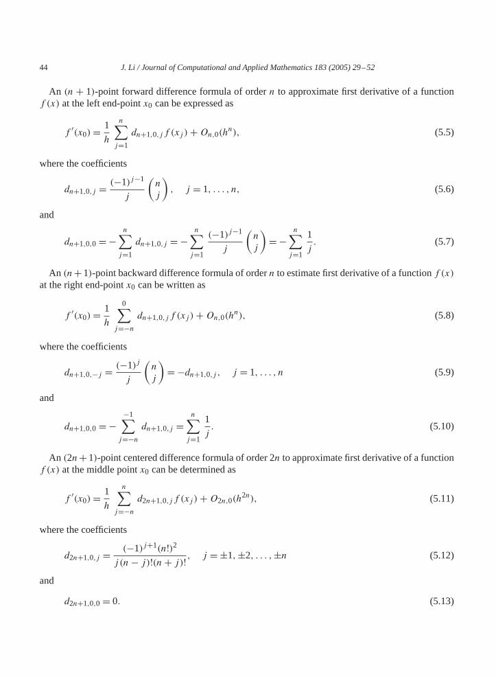
Forward, backward and centered difference formulas are widely used to approximate derivatives inpractice. The forward and backward difference formulas are useful for end-point approximations, partic-ularly with regard to the clamped cubic spline interpolation. For evenly spaced data their general formscan be yielded as follows by use of Corollaries 2.1 and 2.2.
44 J. Li / Journal of Computational and Applied Mathematics 183 (2005) 29–52
An (n + 1)-point forward difference formula of ordern to approximate first derivative of a functionf (x) at the left end-pointx0 can be expressed as
f ′(x0)= 1
h
n∑j=1
dn+1,0,j f (xj )+On,0(hn), (5.5)
where the coefficients
dn+1,0,j = (−1)j−1
j
(n
j
), j = 1, . . . , n, (5.6)
and
dn+1,0,0 = −n∑j=1
dn+1,0,j = −n∑j=1
(−1)j−1
j
(n
j
)= −
n∑j=1
1
j. (5.7)
An (n+ 1)-point backward difference formula of ordern to estimate first derivative of a functionf (x)at the right end-pointx0 can be written as
f ′(x0)= 1
h
0∑j=−n
dn+1,0,j f (xj )+On,0(hn), (5.8)
where the coefficients
dn+1,0,−j = (−1)j
j
(n
j
)= −dn+1,0,j , j = 1, . . . , n (5.9)
and
dn+1,0,0 = −−1∑j=−n
dn+1,0,j =n∑j=1
1
j. (5.10)
An (2n+ 1)-point centered difference formula of order 2n to approximate first derivative of a functionf (x) at the middle pointx0 can be determined as
f ′(x0)= 1
h
n∑j=−n
d2n+1,0,j f (xj )+O2n,0(h2n), (5.11)
where the coefficients
d2n+1,0,j = (−1)j+1(n!)2j (n− j)!(n+ j)! , j = ±1,±2, . . . ,±n (5.12)
and
d2n+1,0,0 = 0. (5.13)
J. Li / Journal of Computational and Applied Mathematics 183 (2005) 29–52 45
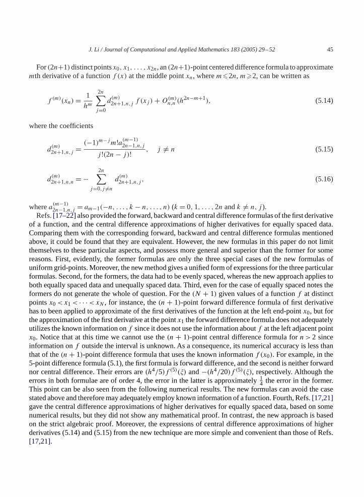
For(2n+1)distinct pointsx0, x1, . . . , x2n, an(2n+1)-point centered difference formula to approximatemth derivative of a functionf (x) at the middle pointxn, wherem�2n,m�2, can be written as
f (m)(xn)= 1
hm
2n∑j=0
d(m)2n+1,n,j f (xj )+O(m)n,n (h2n−m+1), (5.14)
where the coefficients
d(m)2n+1,n,j = (−1)m−jm!a(m−1)
2n−1,n,j
j !(2n− j)! , j �= n (5.15)
d(m)2n+1,n,n = −
2n∑j=0,j �=n
d(m)2n+1,n,j , (5.16)
wherea(m−1)2n−1,n,j = am−1(−n, . . . , k − n, . . . , n) (k = 0,1, . . . ,2n andk �= n, j ).
Refs.[17–22]also provided the forward, backward and central difference formulas of the first derivativeof a function, and the central difference approximations of higher derivatives for equally spaced data.Comparing them with the corresponding forward, backward and central difference formulas mentionedabove, it could be found that they are equivalent. However, the new formulas in this paper do not limitthemselves to these particular aspects, and possess more general and superior than the former for somereasons. First, evidently, the former formulas are only the three special cases of the new formulas ofuniform grid-points. Moreover, the new method gives a unified form of expressions for the three particularformulas. Second, for the formers, the data had to be evenly spaced, whereas the new approach applies toboth equally spaced data and unequally spaced data. Third, even for the case of equally spaced notes theformers do not generate the whole of question. For the(N + 1) given values of a functionf at distinctpointsx0<x1< · · ·<xN , for instance, the(n + 1)-point forward difference formula of first derivativehas to been applied to approximate of the first derivatives of the function at the left end-pointx0, but forthe approximation of the first derivative at the pointx1 the forward difference formula does not adequatelyutilizes the known information onf since it does not use the information aboutf at the left adjacent pointx0. Notice that at this time we cannot use the(n + 1)-point central difference formula forn>2 sinceinformation onf outside the interval is unknown. As a consequence, its numerical accuracy is less thanthat of the(n+ 1)-point difference formula that uses the known informationf (x0). For example, in the5-point difference formula (5.1), the first formula is forward difference, and the second is neither forwardnor central difference. Their errors are(h4/5)f (5)(�) and−(h4/20)f (5)(�), respectively. Although theerrors in both formulae are of order 4, the error in the latter is approximately1
4 the error in the former.This point can be also seen from the following numerical results. The new formulas can avoid the casestated above and therefore may adequately employ known information of a function. Fourth, Refs.[17,21]gave the central difference approximations of higher derivatives for equally spaced data, based on somenumerical results, but they did not show any mathematical proof. In contrast, the new approach is basedon the strict algebraic proof. Moreover, the expressions of central difference approximations of higherderivatives (5.14) and (5.15) from the new technique are more simple and convenient than those of Refs.[17,21].
46 J. Li / Journal of Computational and Applied Mathematics 183 (2005) 29–52
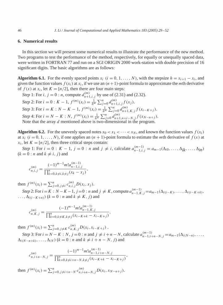
6. Numerical results
In this section we will present some numerical results to illustrate the performance of the new method.Two programs to test the performance of the method, respectively, for equally or unequally spaced data,were written in FORTRAN 77 and run on a SGI ORIGIN 2000 work-station with double precision of 16significant digits. The basic algorithms are as follows:
Algorithm 6.1. For the evenly spaced pointsxi (i = 0,1, . . . , N), with the stepsizeh= xi+1 − xi , andgiven the function valuesf (xi) atxi , if we use an(n+1)-point formula to approximate themth derivativeof f (x) atxi , letK = [n/2], then there are four main steps:
Step1: Fori, j = 0 : n, computed(m)n+1,i,j by use of (2.31) and (2.32).
Step2: Fori = 0 : K − 1, f (m)(xi)= 1hm
∑nj=0 d
(m)n+1,i,j f (xj ).
Step3: Fori =K : N −K − 1, f (m)(xi)= 1hm
∑nj=0 d
(m)n+1,K,jf (xi−K+j ).
Step4: Fori =N −K : N , f (m)(xi)= 1hm
∑nj=0 d
(m)n+1,n+i−N,jf (xN−n+j ).
Note that the arrayd mentioned above is two-dimensional in the program.
Algorithm 6.2. For the unevenly spaced notesx0<x1< · · ·<xN , and known the function valuesf (xi)atxi (i = 0,1, . . . , N), if one applies an(n+ 1)-point formula to estimate themth derivative off (x) atxi , letK = [n/2], then three critical steps contain:
Step1: For i = 0 : K − 1, j = 0 : n andj �= i, calculatea(m−1)n−1,i,j = am−1(�i0, . . . ,�ik, . . . ,�in)
(k = 0 : n andk �= i, j ) and
c(m)n,i,j = (−1)m−1m!a(m−1)
n−1,i,j∏nk=0,k �=i,k �=j (xk − xj ) ,
thenf (m)(xi)= ∑nj=0,j �=i c
(m)n,i,jD(xi, xj ).
Step2: Fori=K : N−K−1,j=0 : n andj �= K, computea(m−1)n−1,K,j=am−1(�i(i−K), . . . ,�i(i−K+k),
. . . ,�i(i−K+n)) (k = 0 : n andk �= K, j ) and
c(m)n,K,j = (−1)m−1m!a(m−1)
n−1,K,j∏nk=0,k �=K,k �=j (xi−K+k − xi−K+j )
,
thenf (m)(xi)= ∑nj=0,j �=K c
(m)n,K,jD(xi, xi−K+j ) .
Step3: Fori=N −K : N , j =0 : n andj �= i+n−N , calculatea(m−1)n−1,i+n−N,j =am−1(�i(N−n), . . . ,
�i(N−n+k), . . . ,�iN ) (k = 0 : n andk �= i + n−N, j ) and
c(m)n,i+n−N,j = (−1)m−1m!a(m−1)
n−1,i+n−N,j∏nk=0,k �=i+n−N,k �=j (xi−K+k − xi−K+j )
,
thenf (m)(xi)= ∑nj=0,j �=i+n−N c
(m)n,i+n−N,jD(xi, xN−n+j ).

J. Li / Journal of Computational and Applied Mathematics 183 (2005) 29–52 47
Table 1Error in difference approximation tof ′(x) for equally spaced data
i x(i) (n+ 1)-point formula
7-points 8-points 9-points 10-points 11-points
0 0.00 1.82E− 07 2.67E− 09 1.49E− 09 4.94E− 11 8.15E− 121 0.03 3.03E− 08 4.09E− 10 1.86E− 10 5.57E− 12 8.21E− 132 0.06 1.21E− 08 1.45E− 10 5.28E− 11 1.41E− 12 1.82E− 133 0.09 9.06E− 09 9.26E− 11 2.63E− 11 6.16E− 13 6.93E− 144 0.12 8.87E− 09 1.40E− 10 2.10E− 11 4.20E− 13 3.64E− 145 0.15 8.58E− 09 1.85E− 10 2.01E− 11 4.88E− 13 2.75E− 146 0.18 8.21E− 09 2.29E− 10 1.92E− 11 4.97E− 13 3.82E− 147 0.21 7.75E− 09 2.33E− 10 2.38E− 11 7.55E− 13 6.62E− 148 0.24 1.02E− 08 3.96E− 10 4.73E− 11 1.78E− 12 1.71E− 139 0.27 2.54E− 08 1.21E− 09 1.65E− 10 7.19E− 12 8.10E− 13
10 0.30 1.51E− 07 8.64E− 09 1.31E− 09 6.57E− 11 7.85E− 12
Notice please that all of the symbolsa, c, andD stated above are only one-dimensional arrays aboutthe indexj in the program.
The example function is
f (x)= xeax + sinbx, (6.1)
wherea=−2 andb=3.Then its first, second, third and fourth derivatives aref ′(x)=(1+a)xeax+b cosbx,f ′′(x)= a(2+ a)xeax − b2 sinbx, f ′′′(x)= a2(3+ a)xeax − b3 cosbx, andf (4)(x)= a3(4+ a)xeax +b4 sinbx, respectively. Based on the algorithms mentioned above, we have carried out the(n+ 1)-pointformulas, wheren is from 1 to 10, to approximate the first, second, third and fourth derivatives off (x)
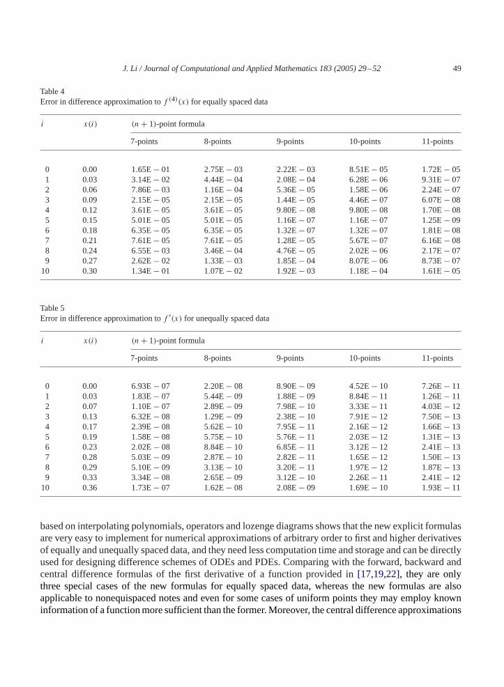
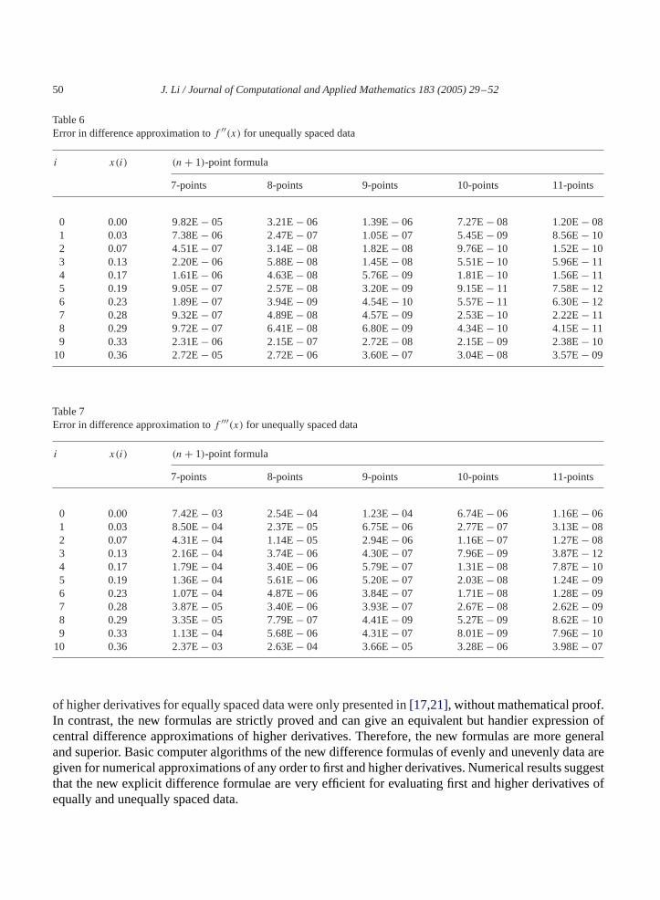
for two cases, the equally and unequally spaced data. To save space, we only show the numerical resultsof the (n + 1)-point formulas, wheren is from 6 to 10.Tables 1–4, respectively, represent errors indifference approximation to the first, second, third and fourth derivatives off (x) for equally spaced datawith the stepsizeh = 0.03.Tables 5–8illustrate, respectively, errors in difference approximation to thefirst, second, third and fourth derivatives off (x) for unequally spaced data. From the tables, evidently,some conclusions can be given as follows:
(1) The new method performs well whether the data are equally spaced or unequally spaced, and whetherthe derivative is first or higher orders.
(2) In general, using more evaluation points produces greater accuracy. That is to say, increasing theorder of numerical differentiation, reduces the error.
(3) Givenn, the accuracies of the(n + 1)-point forward and backward difference approximations areobviously less than those of the other(n + 1)-point formulas. This is because the(n + 1)-pointforward and backward formulas use data on only one side of reference point and the other(n+ 1)-point formulas use data on both sides of reference point.

48 J. Li / Journal of Computational and Applied Mathematics 183 (2005) 29–52
Table 2Error in difference approximation tof ′′(x) for equally spaced data
i x(i) (n+ 1)-point formula
7-points 8-points 9-points 10-points 11-points
0 0.00 2.97E− 05 4.49E− 07 2.70E− 07 9.25E− 09 1.58E− 091 0.03 2.59E− 06 3.77E− 08 1.97E− 08 6.33E− 10 9.96E− 112 0.06 4.72E− 07 6.99E− 09 3.36E− 09 1.02E− 10 1.50E− 113 0.09 1.19E− 09 1.19E− 09 7.96E− 10 2.48E− 11 3.30E− 124 0.12 1.99E− 09 1.99E− 09 5.40E− 12 5.40E− 12 9.15E− 135 0.15 2.76E− 09 2.76E− 09 6.52E− 12 6.52E− 12 3.48E− 136 0.18 3.50E− 09 3.50E− 09 7.39E− 12 7.39E− 12 1.31E− 127 0.21 4.19E− 09 4.19E− 09 7.05E− 10 3.20E− 11 3.53E− 128 0.24 3.92E− 07 2.12E− 08 2.98E− 09 1.31E− 10 1.45E− 119 0.27 2.16E− 06 1.19E− 07 1.74E− 08 8.31E− 10 9.71E− 11
10 0.30 2.46E− 05 1.50E− 06 2.37E− 07 1.24E− 08 1.51E− 09
Table 3Error in difference approximation tof ′′′(x) for equally spaced data
i x(i) (n+ 1)-point formula
7-points 8-points 9-points 10-points 11-points
0 0.00 2.74E− 03 4.31E− 05 2.92E− 05 1.05E− 06 1.95E− 071 0.03 8.21E− 05 7.93E− 07 2.20E− 08 6.83E− 09 2.22E− 092 0.06 9.40E− 05 1.06E− 06 3.23E− 07 7.61E− 09 7.84E− 103 0.09 8.22E− 05 8.49E− 07 2.30E− 07 5.14E− 09 5.47E− 104 0.12 8.05E− 05 1.28E− 06 1.99E− 07 3.99E− 09 3.59E− 105 0.15 7.79E− 05 1.69E− 06 1.91E− 07 4.64E− 09 3.00E− 106 0.18 7.45E− 05 2.08E− 06 1.82E− 07 4.69E− 09 3.35E− 107 0.21 7.03E− 05 2.11E− 06 2.08E− 07 6.21E− 09 5.10E− 108 0.24 8.00E− 05 2.73E− 06 2.92E− 07 9.17E− 09 7.75E− 109 0.27 7.10E− 05 1.35E− 06 3.45E− 09 1.12E− 08 2.10E− 09
10 0.30 2.25E− 03 1.53E− 04 2.54E− 05 1.43E− 06 1.84E− 07
7. Conclusion
General explicit finite difference formulas for numerical derivatives of unequally and equally spaceddata are studied in this paper. Through introducing the generalized Vandermonde determinant, the linearalgebraic system of a kind of Vandermonde equations is solved analytically by use of the basic propertiesof the determinant, and then combining with Taylor series general explicit finite difference formulaswith arbitrary order accuracy for approximating first and higher derivates of a function are presentedfor unequally or equally spaced grid-points. A comparison with other implicit finite difference formulas
J. Li / Journal of Computational and Applied Mathematics 183 (2005) 29–52 49
Table 4Error in difference approximation tof (4)(x) for equally spaced data
i x(i) (n+ 1)-point formula
7-points 8-points 9-points 10-points 11-points
0 0.00 1.65E− 01 2.75E− 03 2.22E− 03 8.51E− 05 1.72E− 051 0.03 3.14E− 02 4.44E− 04 2.08E− 04 6.28E− 06 9.31E− 072 0.06 7.86E− 03 1.16E− 04 5.36E− 05 1.58E− 06 2.24E− 073 0.09 2.15E− 05 2.15E− 05 1.44E− 05 4.46E− 07 6.07E− 084 0.12 3.61E− 05 3.61E− 05 9.80E− 08 9.80E− 08 1.70E− 085 0.15 5.01E− 05 5.01E− 05 1.16E− 07 1.16E− 07 1.25E− 096 0.18 6.35E− 05 6.35E− 05 1.32E− 07 1.32E− 07 1.81E− 087 0.21 7.61E− 05 7.61E− 05 1.28E− 05 5.67E− 07 6.16E− 088 0.24 6.55E− 03 3.46E− 04 4.76E− 05 2.02E− 06 2.17E− 079 0.27 2.62E− 02 1.33E− 03 1.85E− 04 8.07E− 06 8.73E− 07
10 0.30 1.34E− 01 1.07E− 02 1.92E− 03 1.18E− 04 1.61E− 05
Table 5Error in difference approximation tof ′(x) for unequally spaced data
i x(i) (n+ 1)-point formula
7-points 8-points 9-points 10-points 11-points
0 0.00 6.93E− 07 2.20E− 08 8.90E− 09 4.52E− 10 7.26E− 111 0.03 1.83E− 07 5.44E− 09 1.88E− 09 8.84E− 11 1.26E− 112 0.07 1.10E− 07 2.89E− 09 7.98E− 10 3.33E− 11 4.03E− 123 0.13 6.32E− 08 1.29E− 09 2.38E− 10 7.91E− 12 7.50E− 134 0.17 2.39E− 08 5.62E− 10 7.95E− 11 2.16E− 12 1.66E− 135 0.19 1.58E− 08 5.75E− 10 5.76E− 11 2.03E− 12 1.31E− 136 0.23 2.02E− 08 8.84E− 10 6.85E− 11 3.12E− 12 2.41E− 137 0.28 5.03E− 09 2.87E− 10 2.82E− 11 1.65E− 12 1.50E− 138 0.29 5.10E− 09 3.13E− 10 3.20E− 11 1.97E− 12 1.87E− 139 0.33 3.34E− 08 2.65E− 09 3.12E− 10 2.26E− 11 2.41E− 12
10 0.36 1.73E− 07 1.62E− 08 2.08E− 09 1.69E− 10 1.93E− 11
based on interpolating polynomials, operators and lozenge diagrams shows that the new explicit formulasare very easy to implement for numerical approximations of arbitrary order to first and higher derivativesof equally and unequally spaced data, and they need less computation time and storage and can be directlyused for designing difference schemes of ODEs and PDEs. Comparing with the forward, backward andcentral difference formulas of the first derivative of a function provided in[17,19,22], they are onlythree special cases of the new formulas for equally spaced data, whereas the new formulas are alsoapplicable to nonequispaced notes and even for some cases of uniform points they may employ knowninformation of a function more sufficient than the former. Moreover, the central difference approximations
50 J. Li / Journal of Computational and Applied Mathematics 183 (2005) 29–52
Table 6Error in difference approximation tof ′′(x) for unequally spaced data
i x(i) (n+ 1)-point formula
7-points 8-points 9-points 10-points 11-points
0 0.00 9.82E− 05 3.21E− 06 1.39E− 06 7.27E− 08 1.20E− 081 0.03 7.38E− 06 2.47E− 07 1.05E− 07 5.45E− 09 8.56E− 102 0.07 4.51E− 07 3.14E− 08 1.82E− 08 9.76E− 10 1.52E− 103 0.13 2.20E− 06 5.88E− 08 1.45E− 08 5.51E− 10 5.96E− 114 0.17 1.61E− 06 4.63E− 08 5.76E− 09 1.81E− 10 1.56E− 115 0.19 9.05E− 07 2.57E− 08 3.20E− 09 9.15E− 11 7.58E− 126 0.23 1.89E− 07 3.94E− 09 4.54E− 10 5.57E− 11 6.30E− 127 0.28 9.32E− 07 4.89E− 08 4.57E− 09 2.53E− 10 2.22E− 118 0.29 9.72E− 07 6.41E− 08 6.80E− 09 4.34E− 10 4.15E− 119 0.33 2.31E− 06 2.15E− 07 2.72E− 08 2.15E− 09 2.38E− 10
10 0.36 2.72E− 05 2.72E− 06 3.60E− 07 3.04E− 08 3.57E− 09
Table 7Error in difference approximation tof ′′′(x) for unequally spaced data
i x(i) (n+ 1)-point formula
7-points 8-points 9-points 10-points 11-points
0 0.00 7.42E− 03 2.54E− 04 1.23E− 04 6.74E− 06 1.16E− 061 0.03 8.50E− 04 2.37E− 05 6.75E− 06 2.77E− 07 3.13E− 082 0.07 4.31E− 04 1.14E− 05 2.94E− 06 1.16E− 07 1.27E− 083 0.13 2.16E− 04 3.74E− 06 4.30E− 07 7.96E− 09 3.87E− 124 0.17 1.79E− 04 3.40E− 06 5.79E− 07 1.31E− 08 7.87E− 105 0.19 1.36E− 04 5.61E− 06 5.20E− 07 2.03E− 08 1.24E− 096 0.23 1.07E− 04 4.87E− 06 3.84E− 07 1.71E− 08 1.28E− 097 0.28 3.87E− 05 3.40E− 06 3.93E− 07 2.67E− 08 2.62E− 098 0.29 3.35E− 05 7.79E− 07 4.41E− 09 5.27E− 09 8.62E− 109 0.33 1.13E− 04 5.68E− 06 4.31E− 07 8.01E− 09 7.96E− 10
10 0.36 2.37E− 03 2.63E− 04 3.66E− 05 3.28E− 06 3.98E− 07
of higher derivatives for equally spaced data were only presented in[17,21], without mathematical proof.In contrast, the new formulas are strictly proved and can give an equivalent but handier expression ofcentral difference approximations of higher derivatives. Therefore, the new formulas are more generaland superior. Basic computer algorithms of the new difference formulas of evenly and unevenly data aregiven for numerical approximations of any order to first and higher derivatives. Numerical results suggestthat the new explicit difference formulae are very efficient for evaluating first and higher derivatives ofequally and unequally spaced data.

J. Li / Journal of Computational and Applied Mathematics 183 (2005) 29–52 51
Table 8Error in difference approximation tof (4)(x) for unequally spaced data
i x(i) (n+ 1)-point formula
7-points 8-points 9-points 10-points 11-points
0 0.00 3.55E− 01 1.30E− 02 7.45E− 03 4.38E− 04 8.31E− 051 0.03 1.09E− 01 3.51E− 03 1.38E− 03 6.87E− 05 1.05E− 052 0.07 1.42E− 02 5.28E− 04 2.20E− 04 1.08E− 05 1.54E− 063 0.13 1.00E− 02 3.04E− 04 7.57E− 05 2.78E− 06 2.71E− 074 0.17 9.86E− 03 3.60E− 04 4.18E− 05 1.50E− 06 1.37E− 075 0.19 4.41E− 03 3.78E− 05 1.61E− 05 1.80E− 07 3.75E− 086 0.23 7.82E− 04 9.42E− 05 1.05E− 06 4.37E− 07 5.32E− 087 0.28 6.20E− 03 2.83E− 04 2.26E− 05 8.96E− 07 5.26E− 088 0.29 7.81E− 03 5.34E− 04 5.60E− 05 3.43E− 06 3.15E− 079 0.33 2.99E− 02 2.58E− 03 3.12E− 04 2.30E− 05 2.45E− 06
10 0.36 1.34E− 01 1.73E− 02 2.59E− 03 2.53E− 04 3.21E− 05
Acknowledgements
This work was supported jointly by the NSFC projects (Grant Nos. 40325015, 40221503, and 49905007).
References
[1] R.S. Anderssen, P. Bloomfield, Numerical differentiation procedures for non-exact data, Numer. Math. 22 (1973/74)157–182.
[2] R.L. Burden, J.D. Faires, Numerical Analysis, seventh ed., Brooks/Cole, Pacific Grove, CA, 2001.[3] S.C. Chapra, R.P. Canale, Numerical Methods for Engineers, third ed., McGraw-Hill, New York, 1998.[4] L. Collatz, The Numerical Treatment of Differential Equations, third ed., Springer, Berlin, 1966.[5] G. Corliss, C. Faure, A. Griewank, L. Hascoet, U. Naumann, Automatic Differentiation of Algorithms—From Simulation
to Optimization, Springer, Berlin, 2002.[6] J. Cullum, Numerical differentiation and regularization, SIAM J. Numer. Anal. 8 (2) (1971) 254–265.[7] G. Dahlquist, A. Bjorck, Numerical Methods, Prentice-Hall, Inc., Englewood Cliffs, NJ, 1974.[8] T. Dokken, T. Lyche, A divided difference formula for the error in Hermite interpolation, BIT 19 (1979) 539–540.[9] W. Forst, Interpolation und numerische differentiation, J. Approx. Theory 39 (2) (1983) 118–131.
[10] C.F. Gerald, P.O. Wheatley, Applied Numerical Analysis, fourth ed., Addison-Wesley Pub. Co., Reading, MA, 1989.[11] L.P. Grabar, Numerical differentiation by means of Chebyshev polynomials orthonormalized on a system of equidistant
points, Zh. Vychisl, Mat. i Mat. Fiz. 7 (6) (1967) 1375–1379.[12] A. Griewank, Evaluating Derivatives, Principles and Techniques of Algorithmic Differentiation, Number 19 in Frontiers
in Applied Mathematics, SIAM, Philadelphia, 2000.[13] A. Griewank, F. Corliss, Automatic Differentiation of Algorithms—Theory, Implementation and Application, SIAM,
Philadelphia, 1991.[14] R.W. Hamming, Numerical Methods for Scientists and Engineers, McGraw-Hill, New York, 1962.[15] M. Hanke, O. Scherzer, Inverse problems light—numerical differentiation, Amer. Math. Monthly 6 (2001) 512–522.[16] M.T. Heath, Science Computing—An Introductory Survey, second ed., McGraw-Hill, New York, 1997.[17] I.R. Khan, R. Ohba, Closed-form expressions for the finite difference approximations of first and higher derivatives based
on Taylor series, J. Comput. Appl. Math. 107 (1999) 179–193.
52 J. Li / Journal of Computational and Applied Mathematics 183 (2005) 29–52
[18] I.R. Khan, R. Ohba, Digital differentiators based on Taylor series, IEICE Trans. Fund. E82-A (12) (1999) 2822–2824.[19] I.R. Khan, R. Ohba, New finite difference formulas for numerical differentiation, J. Comput. Appl. Math. 126 (2001)
269–276.[20] I.R. Khan, R. Ohba, Mathematical proof of explicit formulas for tap-coefficients of Taylor series based FIR digital
differentiators, IEICE Trans. Fund. E84-A (6) (2001) 1581–1584.[21] I.R. Khan, R. Ohba, Taylor series based finite difference approximations of higher-degree derivatives, J. Comput. Appl.
Math. 154 (2003) 115–124.[22] I.R. Khan, R. Ohba, N. Hozumi, Mathematical proof of closed form expressions for finite difference approximations based
on Taylor series, J. Comput. Appl. Math. 150 (2003) 303–309.[23] T. King, D. Murio, Numerical differentiation by finite dimensional regularization, IMA J. Numer. Anal. 6 (1986) 65–85.[24] I. Knowles, R. Wallace, A variational method for numerical differentiation, Numer. Math. 70 (1995) 91–110.[25] E. Kreyzig, Advanced Engineering Mathematics, seventh ed., Wiley, New York, 1994.[26] T.N. Krishnamurti, L. Bounoua, An Introduction to Numerical Weather Prediction Technique Techniques, CRC Press,
Boca Raton, FL, 1995.[27] B.I. Kvasov, Numerical differentiation and integration on the basis of interpolation parabolic splines, Chisl. Metody Mekh.
Sploshn. Sredy 14 (2) (1983) 68–80.[28] J.H. Mathews, K.D. Fink, Numerical Methods Using MATLAB, third ed., Prentice-Hall, Inc., Englewood Cliffs, NJ, 1999.[29] D.A. Murio, The Mollification Method and the Numerical Solution of Ill-posed Problems, Wiley, New York, 1993.[30] L.B. Rail, Automatic Differentiation—Techniques and Applications, Springer, Berlin, 1981.[31] A.G. Ramm, On numerical differentiation, Mathem. Izvestija vuzov 11 (1968) 131–135.[32] A.G. Ramm, Stable solutions of some ill-posed problems, Math. Meth. Appl. Sci. 3 (1981) 336–363.[33] P. Silvester, Numerical formation of finite-difference operators, IEEE Trans. Microwave Theory Technol. MTT-18 (10)
(1970) 740–743.[34] A.N. Tikhonov, V.Y. Arsenin, Solutions of Ill-posed Problems, Wiley, New York, 1977.[35] V.V. Vasin, Regularization of the problem of numerical differentiation, Matem. zap. Ural’skii univ. 7 (2) (1969) 29–33.[36] V.V. Vershinin, N.N. Pavlov, Approximation of derivatives by smoothing splines, Vychisl. Sistemy 98 (1983) 83–91.[37] G. Wahba, Spline Models for Observational Data, SIAM, Philadelphia, 1990.