106

ANALYSIS OF EXPLICIT FINITE DIFFERENCE METHODS USED IN COMPUTATIONAL FLUID MECHANICS

John Noye

1. INTRODUCTION It is now commonplace to simulate fluid motion by numerically

solving the governing partial differential equations on high speed

digital computers.

Finite difference techniques, because of their relative simplicity

and their long history of successful application, are the most commonly

used. They have, for example, been used in depth-averaged and three­

dimensional time dependent tidal modelling by many oceanographers and

coastal engineers: see, for example, Noye and Tronson (1978), Noye

et. al. (1982) and Noye (1984a).

However, like finite element techniques and boundary integral

methods, finite difference methods of solving the Eulerian equations of

hydrodynamics seldom model the advective terms accurately. Errors in

the phase and amplitude of waves are usual, particularly the former.

The accuracy of various explicit finite difference methods applied

to solving the advection equation, namely

(1.1) ~~ + u~~ = 0, 0 S x S 1, t > 0, u a positive constant,

is investigated in this work. The boundary condition to be used in

practice is that T(O,t) is defined for t > 0, with no values prescribed

at x = 1.

The von Neumann amplication factor is not only used to find the

stability criteria of the methods investigated, but also to determine

the wave deformation properties of the technique. These properties are

then linked to the "modified" equation; that is, the partial differen­

tial equation which is equivalent to the finite difference equation,

after the former has been modified so it contains only the one temporal

derivative, dT/dt, all other derivatives being spatial.

It will be seen that successively more accurate methods can be

developed by systematic elimination of the higher order terms in the

truncation error, which is the difference between the modified equation

and the given equation (1.1).

107

The approach used by Molenkamp (1968) and Crowley (1968) to assess

oche accuracy of the numerical method to ·the advection equation is also

used to illus·trate the conclusions reached from the ma-thematical analy­

sis; that is, the numerical method is applied to a simple problem whose

exact solution is knmvn, and the numerical solu·tion is compared with

the exact solution. The problem chosen is that of an infinite train of

Gaussian pulses, used as ir.i·tial condition to (1.1), for which the exact

solution at time t on the infinite domain --oo < x < co is the same ·train

displaced a dis·tance ut to the right along the x-axis. The corresponding

numerical solu·tion of ochis process is obtained using cyclic boundary

conditions at x = 0 and x = 1.

Higher order teclli,iques, such as the third order upwind biassed

method and Rusanov' s methods, are clearly more accurate than t:he

more widely used methods such as first order upwind and the Lax-Wendroff

methods. The increased accuracy justifies the increased computa·tional

time and complications near the boundary due to extension of the compu­

'cat.ional molecule for cert.ain higher order methods.

2. THE FIRST-ORDER UPWIND METHOD At the gridpoint (j6x,nL'I·t), j

L'lx 1/J, the advection equa·tion

(2.1) ClTin + Clt . J

-,n dT u­Clx .

J

o,

l, 2, . ., J, n

becomes, on using ·the two-point forward time approximation and the two­

point backward space approximation,

Tn.+l n n n - T. T. - T. l

(2,2) 1 J + u{ J J- } = 0. L'lt L'lx

On rearrangement, this gives 'che two point upwind equation, see Godunov (1959),

(2.3) n+l

T. J

n CT. _ +

J-1.

where T~ is an approxima·tion to T (j6x, nL'It) and c J

Courant nuzaber.

uL'It/L'Ix > 0 is the

The amplification factor, G(c,NA), of the von Neumann method of

stability analysis is obtained by substitu·ting Tr: = (G) nexp{i (2"ITj/N))}, J \

i = /-1, into (2.3), where the parameter N;.. is the number of grid-

108

spacings per waveleng·th of a particular Fourie1~ mode contained in ~che

initial conditions. For this me·thod we obtain

(2. 4)

The stabili'cy requirement is tha·t I G I ,; 1 for all

so long as 0 < c ~ l.

}.

2: 2, which. is true

The amplification fac·tor also yields information about 'che differ-

ence be'cween the numerical and exaci: solutions for an initial condition

consisting of an infinite sine wave of >vaveleng··th NA 1'-x. While t:he ad­

vection equation (L 1) propa•:;ra'ces ·this wave at speed u and unchanged

amplitude, a finite difference equation may transmit 'che t•lave at another

speed and a different amplitude. These effects of t.he fini·te differ-

ence method may be described by two parameters, the relat.ive wave speed

and the amplitude attenua,tion which occurs in one wave period. The

relative wave speed is denoted and defined by

(2. 5) ).1 = u /u = -N, Arg{G (c,N,) N A /1.

and the amplit;ude a-ttenua·tion per •v1ave per:Lod is given by

(2. 6) y

(see 1\loye, l984b, p.l93).

The wave deformation parcuneters, ).1 and y, of the first order up-

voind equation (2.3) are graphed against for various c, in Figure lo

!/lave

109

'rhe loss of amplitude of component vlaves is very large; for instance,

with N~- = 40 and c = 0.4, the amplitude af·ter one '"ave period falls to

0, 7 of i·ts original value, so ·that. af-ter: two wave periods the amplitude

is less than half its original value.

The effec·t of this is seen in Figure 2, in which is shown the

numerical solution after 10 periods for the follm,;ring ·test case. The

initial conditions consis·t of an infinite set of Gaussian peaks (see

dashed curve), symmetrical about x = (P + !,;), P = 0,±1,±2, . , . , so it is - -

periodic in space with pe:ciod l; that is, T (x+l,t) = T (x,t). >-Ji·th

6x = 0. 025 and c = 0, 4, the munerical solution is obtained using cyclic

boundary conditions; tha·t is ';lith T; = j+J' j = 0,1, ... ,J--1. The ex­

cessive \!tiave damping is clear" In spi·te of this, ~~firs~c~order upwinding

is t.he industry s·tandard in chemical, civil and mechanical engineering"

(Leonard, 1981). First-order upwinding is the basic differencing scheme

in many books including Gosman et.aL (1969) and Patankar (1980).

2 solved

The consistency analysis of (2. 3) invo.l<~res Taylor series expansions

of eacb t.erm of the finite difference equa·tion about. ·the gridpCJin·t

(j6x, nf'lt). This yields at ·this gridpoin·t tt.e eq;1ivalent par·cial

differen:tial equa·tion

+

from which mo_y be derived ·the 11 m.odif-Led 1 ~ equci.tion

110

on successive subs-titution of (2, 7) in itself to replace ·the t:emporal

deriva-tives on ·the right. side, by spa.tial derivatives (see Warming and

Hyett, 1974). Clearly ·the fini'ce difference equation (2,3) is consis­

tent with the partial differential equations (l.l), because the right

sides of (2.7) and (2.8) tend to zero as the grid-spacings ~t, ~x both

tend to zero.

Equation (2. 8)' which has the general form

(2. 9) <h (h ::l 2 T 3 3T 3 4T 3 5T -+ u-= cz --- + C3 --+ C4 CJx4 + cs (lx5- + Cl·t dX Clx 2 CJx3

is related to the amplitude response per I!'Jave period y by 'che rela·tion

y

and ·to the relative wave speed ll by

(2.11)

(see Noye, l984b, p.242). Clearly, the coefficien·ts of the even deri-

vatives of x, namely c 2 , c,,, c 5 , ••• , cont.ribute ·to the amplitude error,

whereas ·the odd coefficien-ts c 3 , cs, c7, ... , contribute to the wave

speed error. Thus, if c2 is negative, y is larger ·than l, and the am-

pli·tude of any perturbai:ion >1ill grm11 exponentially as becomes very

large. In such a case, the finite difference equa·tion is unstable.

For ·the first order upwind equation (2. 3) the amplitude response

per wave period is

(2.12) y

+ l(-) as ~ 00 for fixed c in 0 < c L

The relative wave speed is

(2.13) 1211) 2 (1-c) (l-2c) [l 2'IT z(l-12c+12c 2 ) ••• J ]l 1 - - (-) ------ +

'NA 6 NA 20

l (-) for fixed c in 0 < c < ., -+ { } as N +

1(+) for fixed in ., < < 1 A c c

These asymptotic properties of y and ]l for large are seen in Figure 1 ..

111

3. TWO OTHER FINITE DIFFERENCE METHODS If the two-point forward time and two-point centred space approxi­

mations are substituted into Equation (2.1), the following centred space

finite difference equation is obtained:

(3 .1) n+l n n n

T. =~cT. l + T.- ~CT. l J J- J J+

The corresponding modified equation is

(3.2)

Equation (3.2) is consistent with (1.1), but the negative coefficient

of d 2T/dx2 indicates that perturbations will magnify exponentially so

the equation is unstable.

If the three-point backward space approximation is used with the

two-point forward time approximation, the following three-point upwind

finite difference equation is obtained:

(3.3) n+l n n n

T. =-~cT. 2 + 2cT. l + ~(2-3c)T .. J J- )- J

The corresponding modified equation is

(3.4)

which indicates that (3.3) is unstable because, like (3.2), the coeffic­

ient of d2 T/dx2 is always negative.

In spite of their instability, it is seen in the next Section that

Equations (3.1) and (3.3) may be used with (2.3) to give more accurate

finite difference methods than (2.3).

4. SOME HIGHER ORDER METHODS If the modified equations (2.8) and (3.2) are multiplied by c and

(1-c) respectively, then added, the term containing d2 T/dx2 in the trun­

cation error of Equation (2.9) is eliminated. Applying the same procedure

to the finite difference equations (2.3) and (3.1) yields the Lax­

Wendroff equation

(4.1) n+l n + (1-c) (l+c)Tn. - n T. = ~c(l+c)T. 1 , ~c(l-c)T. 1 , J J- J )+

with corresponding modified equation

112

(4. 2)

Equation (4.1) is stable for 0 < c ,:; l.

Graphs of ·the wave propaga·tion parameters of (4.1) are shown in

Figure 3. These p:r:operties are discernable in the results of the Gauss

pulse test, Figure 4, which shows ·the main peak in the numerical solu-

= 40) lagging behind the true solution. The small peak which

appears ahead of the true solution "' 14) is ac·tually trailing

behind the peak at x = 1. 5 in the exact solution.

Fig. 3 : Wave parameters for the Lax-Wendroff method.

Alternatively, the coefficient c in the modified equa·tion may be

made zero by adding equa.t:ions (2.8) and (3.4) multiplied by t.he same

weights as before 11 c and (1-c respectively., \fl1hen ·the finite diffe:cence

equations (2 .. 3) and (3.3) are treated similarly, the optimal ·three-

poin·t upwi~J.d equation is obt::ained:

(4. 3) n+l

T, J

+ ~(1-c) (2-c)T~, -1 J

vJhich is stable for () < c ::; 2 ar1d has the correspondin9 rnodi:.Eied

equation

dT ()i: +

The :result:s of applying

(2·-c) + . ""

~ 3) t_o solve.:: ·the Ga.uss pulse p:t·oblem are shown

in F'ig-ure 5" Com,ponen·t 1,-~aves t.::cavel f a.s·t :Li.l. t::he rrumer ic .al ~30llJ.-tion

113

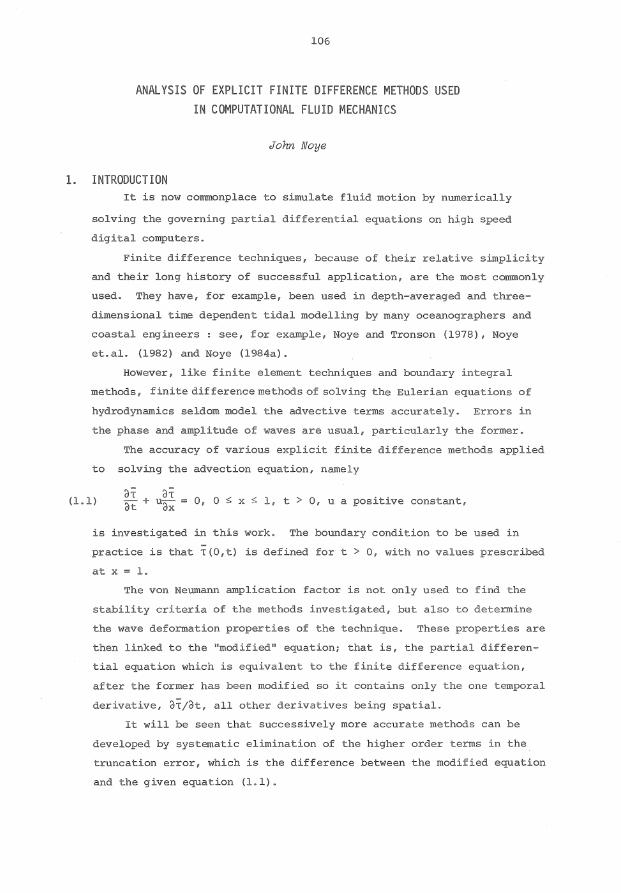
if 0 < c < 1, which is in accord with the fac·t that ·the coefficient of

Cl 3 TjClx 3 (c 3 of Equa·tion (2.9)) is positive.

0 "' N

!:?

4

--EXACT SOLUT!OW - NUfiER I CfiL APPAGJW~AY lOll

test zuith meth.od.

0 "' ol

i :-

~.

method.

I l I \ l l I I

!. 0

o. 5

test uJith

W'e have seen ~chat., for 0 < c < l 11 the finite differ(~:t.~.ce equa·tion

(4 .1) propagates component waves ·too slovlly 1o~hereas (4. 3) propagates

·them too quickly. Taking the ari·thmetic mean of ·these t\'.70 equat.iOI1S

v.Jould gisJe a wave speed v1hich is nearer ~che exac"t value~ rrhi.s yields

Fromm's (1968} !lzero-average 11 phase error 1nethod 1 stable for 0 < c 5 lr

(4. 5) j

in Vlhich t.:he coefficien:'c C3 Of ·the derivat.ive 8- of t.he t.ru.ncation

error in (2.9) is smaller ·than t.hose in (4.2) and (4.4). Ho~cvever, the

coefficient of a 1.n ·tb.e modified equation (2., 9) ccs1 be ma.de zero

by muli:iplying (4" 1) by (2-c) /3 and addh:v:j .3) multiplied by (l+c /3"

Tl1e result:. is =:. third-order u,pv;rind biassed equa.tion, s·tc~ble for 0 < c :::; 1,~

(4 0 6) n+l

T j

:!:--c r l-c '1 ( l+c ) T~ .., -:-6 . ' J-.,. l;;c(2-c) ('-1 )T11

~ -c j -1

with the rnodified equation

(4.7) dT + u-­~}.K

+

Cl 4 T (2-c) (l+c) ()xLi.

()5 (2-c) (l+c) (l-2cl T + . __

114

Use of Fromm's equation (4.5) and the upwind biassed equation (4.6)

to solve the Gauss pulse problem {see Figures 6, 7) indicates the super­

iority of both over the Lax-Wendroff and ~ch.e optimal three-point upwind

equations. The peaks in the numerical solutions are now more nearly

aligned with those of the exact solution, part.icularly for the ·third­

order upwind biassed equation. Leonard (1984) sta·tes tha·t, in his

opinion, "'third-order upc~inding is the rational basis for the develop­

men·t of clean and robus·t algori·thms for compu~ca·tional fluid mechanics".

Hmoever, more accurate higher order methods can be derived from (4. 6),

;:; "' "' 0. 5 ~

Fig.6

- - EXACT SOLUTION -NUMERICAl APFROUHATlON

DISTANCE X

Gauss pulse test with Fromm's method~

0. 5

;;; "' "' i

o. 5

F-ig.? Gauss pulse test 1uith 3rd-order upwind biassed method.

Replacing /J..x by -!'ox in (4. 6) and (4. 7) yields the finite difference

equations

'(4.8) j

!c; (l+c) (2+c) + \ (l+c) (2+c) (1-c)Tn 6 j-1 j

l + -c6 (l+c) (J_-c) , ]+2

lzc(2+c) (1-c)T~ ]+l

wit.h corresponding modified partial differential equation

(4. 9) d~T

) (2+c) (1-c) Clx 4

u(frx)4(1+c) d5T + 60 (2+c) (1-c) (1+2c)(lxS +

Since addi·tion of (4.7) mul~ciplied by (2+c)/4 and (4,9) multiplied by

(2-c)/4 eliminates the coefficient of in the modified equa·tions,

t.hen similar operations applied to the fini~ce difference equations (4. 6)

115

and (4.8) yield the four~ch-order accurate equation, see Rusanov (1970)

and Burstein and Mirin (1970):

(4.10) n+1

T j

~(1-c) (l+c) (2+c)T1'? + ~(2-c) (l+c) (2+c)T~ 24 J-2 6 J-l

+ !,(1-c) (2-c) (l+c) (2+c){'- _!c(l-c) (?-c) (2+c\Tn J 6 - .. j+1

+ ~ (1-c) (l+c) {2+c) T~ .., 24 J+~

This is generally referred to as Rusanov' s "Minimum ampli·tude error"

method and is stable for 0 < c ~ 1.

Rusanov' s "minimum phase error"' me·thod may be obtained in a similar

\vay, by eliminating the coefficients of CJ 5 T/ox 5 from (4.7) and (4.9) by

multiplying by (1+2c) (2+c)/l0c and (l-2c) (2-c)/lOc respectively, and

subtracting. Applying ·this procedure to the finite difference equations

(4.6) and (4.8) yields the equation, stable for 0 < c ~ l:

(4.11) n+l

T j

- ~(l-c) (l+c) (1+2c) (2+c) , + -:;10 (2-c) (l+c) (2+c) (l+4c)<J.1_ 1 60 J-2 ~

+ ~(1-c) (2-c) (l+c) (2+c) T~ + 310 (1-c) (2-c) (2+c) (l-4c) T~+l

- J:_(l-c) (l-2c) (2-c) (l+c)T~ 60 ]+2

Results from the use of (4.10) and (4.11) to solve the Gauss pulse

problem are seen in Figu.res 8 and 9. 'rhe improvemen·t in amplitude res·-

ponse of the "minimum amplitude error" method over the third order up­

winding equation (4. 6) is evident, as is the improvemen·t in "ave speed

of the "minimum phase error" method. Although ·the Rusanov equations

appear to involve an additional spatial gridpoin"c compared to the third­

order upwind-biassed equation, the fact that the veloci•cy u may be

either positive or negative in a realistic situation means that, in

prac"cice, they a.ll require tvm spa·tial gridpoints each side of the cen-

tral gridpoin'c. The problems which ·then remain, are ·that, firstly,

va.lues of the dependent variable T at the gridpoint next to the boundary

x = 0 (i.e. j = 1) must be interpolated >tJi·th an accuracy at least that

of the method being used and, secondly, in order to reach a given grid­

point (jllx, nll•c) in x-t space, the initial set of values may need ·to

extend well beyond values at jllx because of the triangular shape of the

coruputational domain. However, these complications are more than com­

pensated for, by the much greater accuracy of the higher order methods.

;; "' .;

0. 5 ~

8

5. SUMJvlARY

116

- - EXACT SOLIJTI ON - NUHE~ICAL APPRiJXHIAT!ON

DISTANCE

Gauss pulse teBt w{th Rusanov 's min. oJnp l i tude error method. -

;; "' "' G. 5 !:i

9

DISTANCE

Gauss pulse test with Rusanov's min.phase e1~ro:r method.

This art.icle reviews in a. sys·tematic fashion some of ·the explicit.

finite difference me·thods of solving the advection equation. u,c:e of the

modified partial differen"cial equation which is equivalent i:o a fini·te

difference equation used to solve the advection equ.a·tion, con·tains in

the truncat.ion error terms of the form c p

The even

indexed terms coni:ribu·te to ·the error in amplitude response." y ~ and the

odd indexed terms con·tribute to the error in rela·tive vvave speed,, lJ" By

successively eliminating ·these ·t-eJ::-msi' it has been shown ·that methods of

increasing order of accuracy are obtained .. rrhis procedure cc-~.n be con-

tinued, in order ·to produce even more accura.t.e schemes in v1hich )che

spurious oscilla·tions are alinost eliminateCL This is the subject of a

further ar-ticle on this work.

AC KNOvll EDGEMEiHS

The au·thoJ:: thanks Pe·ter St:einle, Ker1 Hay"Tnan a~nd J?ra.nk Nf-~ill for com-

pu:tir1g as,sis·tance and s·timulat.inq cl.iscussion about h.is v,7o·r1~ on fi.ni"te

difference me"chods.

117

REFERENCES Burstein, S.A. and Mirin, A.A. (1970), Third order difference methods for

hyperbolic equations, Journal of Computational Physics, Vol.S, pp.547-571.

Crowley, W.P. (1968), Numerical advection experiments, Monthly Weathe~

Review, Vol.96, pp.l-11.

Fromm, J.E. (1968), A method for reducing dispersion in convective difference

schemes, Journal of Computational Physics, Vol.3, pp.l76-189.

Godunov, S.K. (1959), Finite-difference method for numerical computation of

discontinuous solutions of the equations of fluid dynamics, Matem.Sbornik,

Vol.47, pp.271-306. (In Russian)

Gosman, A.D., Pun, W.M., Runchal, A.K., Spalding, D.B., and Wolfstein, M.

(1969), Heat and Mass T~ansfe~ in Reci~culating Flows, Academic Press.

Lax, R., and Wendroff, B. (1964), Difference schemes for hyperbolic equations

with high order of accuracy, Communications on ~e and Applied Mathematics,

Vol.l7, pp.38l-398.

Leonard, B.P. (1981), A survey of finite differences with upwinding for

numerical modelling of the incompressible convective diffusion equation,

in Recent Advances in Nume~ical Methods in Fluids, Vol.2, ed. c. Taylor,

Pineridge Press.

Leonard, B.P. (1984), Third-order upwinding as a rational basis for comput­

ational fluid dynamics, in Computational Techniques and Applications : CTAC-83,

ed. J. Noye and C. Fletcher, North-Holland Publishing Company, Amsterdam,

pp.l06-120.

Molenkamp, C.R. (1968), Accuracy of finite-difference methods applied to

the advection equation, Journal of Applied Meteo~ology, Vol.7, pp.l60-167.

Noye, B.J. (1984a), Wave propagation characteristics of a numerical model

of tidal motion, in Computational Techniques and Applications : CTAC-83,

ed. J. Noye and C. Fletcher, North-Holland Publishing Company, Amsterdam,

pp. 360-374.

Noye, B.J. (i984b), Finite difference techniques for partial differential

equations, in Computational Techniques fo~ Diffe~ential Equations, ed. J. Noye,

North-Holland Publishing Co., pp.95-354.

Noye, B.J., May, R.L., and Teubner, M.D. (1982), A three-dimensional tidal

model for a shallow gulf, in Nume~ical Solutions of Pa~tial Diffe~ential

Equations, ed. J. Noye, North-Holland Publishing Company, Amsterdam, pp.417-436.

118

Noye, B.J., and Tronson, K.C.S. (1978), Finite difference techniques applied

to the simulation of tides and currents in gulfs, in Numeriaal Solution of

Fluid Motion, ed. J. Noye, North-Holland Publishing Company, Amsterdam,

pp.285-355.

Patankar, s.v. (1980), Numeriaal Heat Transfer and Fluid Flow, Hemisphere

Publishing Corporation, McGraw-Hill.

Rusanov, V.V. (1970), On difference schemes of third order accuracy for non­

linear hyperbolic systems, Journal of Computational Physias, Vol.S, pp.507-516.

Warming, R.F., and Hyett, B.J. (1974), The modified equation approach to the

stability and accuracy analysis of finite-difference methods, Journal of

Computational Physias, Vol.l4, pp.l59-179.

Applied Mathematics Department University of Adelaide ADELAIDE SA 5000