Embed Size (px)
Citation preview
GENERAL DISTRIBUTION
OCDE/GD(95)1
ECONOMICS DEPARTMENTWORKING PAPERS
NO. 152
ESTIMATING POTENTIAL OUTPUT, OUTPUT GAPS ANDSTRUCTURAL BUDGET BALANCES
byClaude Giorno, Pete Richardson, Deborah Roseveare
and Paul van den Noord
ORGANISATION FOR ECONOMIC CO-OPERATION AND DEVELOPMENT
Paris 1995
>
COMPLETE DOCUMENT AVAILABLE ON OLIS IN ITS ORIGINAL FORMAT

ESTIMATING POTENTIAL OUTPUT, OUTPUT GAPS ANDSTRUCTURAL BUDGET BALANCES
This paper reviews the methods used for estimating potential output in OECD countries and theuse of the resulting output gaps for the calculation of structural budget balances. The "split time trend"method for estimating trend output that was previously used for calculating structural budget balances iscompared with two alternative methods, smoothing real GDP using a Hodrick Prescott filter and estimatingpotential output using a production function approach. It is concluded that the production function approachfor estimating potential output provides the best method for estimating output gaps and for calculatingstructural budget balances, with the results obtained by smoothing GDP providing a cross check. New taxand expenditure elasticities, along with the potential output gaps, are used to derive structural budgetbalances.
* * * * *
ESTIMATION DE LA PRODUCTION POTENTIELLE, DES ÉCARTS DU PRODUCTION ETLES SOLDES BUDGÉTAIRES STRUCTURELS
Ce document passe en revue les différentes méthodes utilisées pour estimer la productionpotentielle dans les pays de l’OCDE et l’utilisation des écarts de production qui a dêcoulent pour le calculdes soldes budgétaires structurels. La méthode utilisant la segmentation de la tendance temporelle pourestimer la production potentielle et qui servait précédemment á calculer les soldes budgétaires structurelsest comparée à deux autres méthodes : le lissage du PIB réel à l’aide d’un filtre Hodrick-Prescott etl’estimation de la production potentielle sur la base d’une fonction de production. Il en ressort quel’estimation de la production potentielle par l’approche fonction de production a s’avère être la meilleureméthode pour estimer les écarts de production et pour calculer les soldes budgétaires structurels, les résultatsobtenus par lissage du PIB étant utilisés comme moyens de vérification. Pour estimer les soldes budgétairesstructurels, on utilise de nouvelles élasticités des prelevement et des dépenses et les écarts par rapport a laproduction potentielle.
Copyright OECD, 1995.
Applications for permission to reproduce or translate all, or part of, this material should be madeto : Head of Publications Service, OECD, 2 Rue André Pascal, 75775 Paris Cedex 16, France.
2

Table of Contents
I. Introduction . . . . . . . . . . . . . . . . . . . . . . . . . . . . . . . . . . . . . . . . . . . . . . . . . . . . . . . . . . . 5
II. Estimating Potential Output and Output Gaps. . . . . . . . . . . . . . . . . . . . . . . . . . . . . . . . . . . 7
1. Detrending actual output. . . . . . . . . . . . . . . . . . . . . . . . . . . . . . . . . . . . . . . . . . . 7
Split time-trend method. . . . . . . . . . . . . . . . . . . . . . . . . . . . . . . . . . . . . . . . . . . . 7
Smoothing GDP using a Hodrick-Prescott filter. . . . . . . . . . . . . . . . . . . . . . . . . . . 8
2. Estimating potential output. . . . . . . . . . . . . . . . . . . . . . . . . . . . . . . . . . . . . . . . . . 9
3. Comparison of results. . . . . . . . . . . . . . . . . . . . . . . . . . . . . . . . . . . . . . . . . . . . . 12
III. Estimating Structural Budget Balances. . . . . . . . . . . . . . . . . . . . . . . . . . . . . . . . . . . . . . . . 14
1. Tax elasticities . . . . . . . . . . . . . . . . . . . . . . . . . . . . . . . . . . . . . . . . . . . . . . . . . . 15
2. Expenditure elasticities. . . . . . . . . . . . . . . . . . . . . . . . . . . . . . . . . . . . . . . . . . . . 15
3. Structural budget balances: results. . . . . . . . . . . . . . . . . . . . . . . . . . . . . . . . . . . . 16
IV. Conclusions . . . . . . . . . . . . . . . . . . . . . . . . . . . . . . . . . . . . . . . . . . . . . . . . . . . . . . . . . . 16
Annex 1: Determination of Income-tax and Social Security Contributions Elasticities. . . . . . . . 47
References . . . . . . . . . . . . . . . . . . . . . . . . . . . . . . . . . . . . . . . . . . . . . . . . . . . . . . . . . . . . . . 53
3

Tables
1. Contributions to growth in business sector potential output and NAWRUs
2. Growth rates and output gaps under different methods
3. Regression-based tax elasticities
4. Tax elasticities: previous and new
5. Cyclical effects on government spending
6. Unemployment expenditure and total general government expenditure
7. Comparison of actual and structural budget balances
8. Changes in fiscal balances
9. Cyclical budget balances
Box: Decomposition of growth in potential output
Figures
1. Output growth and output gaps
2. General government structural balances as a percentage of trend GDP
Annex Tables
A1. Gross-earnings elasticities of income tax and social security contributions
A2. Output elasticities of income tax and social security contributions in 1991
A3. Output elasticities of income tax and social contributions
4

ESTIMATING POTENTIAL OUTPUT, OUTPUT GAPS ANDSTRUCTURAL BUDGET BALANCES
Claude Giorno, Pete Richardson, Deborah Roseveare and Paul van den Noord1
I. Introduction
1. Measuring productive potential and the position of output in relation to potential (i.e. the outputgap) are important elements in the OECD Secretariat’s economic assessments and provide a number of keyinsights into macroeconomic performance. For the short-term, measures of the size and persistence ofexisting output gaps provide a useful guide to the balance between supply and demand influences and hencethe assessment of inflation pressures2. For the medium term, measures of productive potential -- thosewhich embody information about trend developments in the stock of capital, the labour force andtechnological change -- provide a useful guide to the aggregate supply capabilities of the economy andhence the assessment of the sustainable non-inflationary growth paths of output and employment.
2. Indicators of the output cycle also provide a means of "looking-through" short-term transitoryinfluences, to identify any build-up in underlying imbalances or structural positions in the macroeconomy.This is particularly important for fiscal analysis, where developments in underlying structural budget deficitscontinue to be a cause for concern in many Member countries and estimates of the output gap can be usedto identify and isolate the impact of cyclical factors of the budget. Thus, short-term improvements inbudget positions due to a pick-up in economic activity may be reversed as activity slows down and shouldtherefore not be seen as an underlying improvement in public finances: if underlying structural deficitsimply increasingly unsustainable public debt positions, this indicates the need for effort and specific policyactions to redress the situation. Changes in the structural deficit may also provide some indication of thedegree of stimulus or restraint that the government wishes to provide to demand (fiscal impulse) over andabove that provided by automatic stabilisers3, or a measure of the degree of fiscal consolidation.
1. The authors would like to acknowledge the useful comments and contributions received frommany members of the Economics Department and in particular, Willi Leibfritz, Mike Feiner,Jorgen Elmeskov and Richard Herd. Debbie Bloch, Marie-Christine Bonnefous, Jackie Gardel,Tara Gleeson, and Anick Lotrous provided invaluable technical assistance.
2. Recent OECD work on the links between demand pressure and price and wage inflation issummarised by Elmeskov (1993), Turneret al. (1993) and Turneret al. (forthcoming).
3. As the change in the structural deficit is only a very rough indicator of discretionary policy, otherindicators have been suggested to measure fiscal stance (see Blanchard, 1990).
5
3. Given the importance attached to measures of potential and cyclical positions, the OECDSecretariat has recently completed a major review of the estimation methods used in its conjuncturalassessments and the construction of its indicators of structural budget balances. In the past, two differentforms of analysis have typically been used.
4. First, in its modelling work and country-specific conjunctural assessments, emphasis has beengiven to measures of potential output which are structural and depend on a production function framework,drawing on information concerning the capital stock, working population, trend participation rates, structuralunemployment and factor productivity developments. Such measures may be qualified, sometimes heavily,by the judgement of country specialists in the OECD Secretariat. Specific weight can also be given to theperceived limits to sustainable non-inflationary growth associated with the labour market, making use ofinformation about both actual rates and underlying natural rates of unemployment (more precisely, the so-called non-accelerating wage rate of unemployment, or NAWRU).
5. Second, the OECD Secretariat’s fiscal indicators have previously been based on measures of trendoutput and cycle derived by the application of time-series methods to actual developments in real GDP4.Though parsimonious in the use of information, the previous method used (known as "split time-trend")was relatively mechanical and therefore had some difficulty in dealing with frequent structural changes andsometimes requiredad hocjudgements about the current cycle to keep results within reasonable bounds.It was of particular concern that the split time-trend method’s weaknesses were most apparent for the periodof most interest to policy-makers -- the present and the near future -- and that it took no account of theconstraints to trend growth due to inflation pressures.
6. For these reasons, and because it would seem preferable to use a single indicator in the assessmentof employment and inflation developments and structural budget balances, the OECD Secretariat hasreviewed and revised its estimation methods to provide a single measure of potential output. Specifically,the chosen measure is one which represents the levels of real GDP, and associated rates of growth, whichare sustainable over the medium term at a stable rate of inflation. Nonetheless, it is clear from this workand the wide range of analytic and survey-based indicators which are available, that significant margins oferror are involved in their estimation and use. Reliance therefore cannot wholly be placed on a singlemeasure of potential or trend output and related indicators must therefore be treated with due caution.5
7. Details of the method the Secretariat has now adopted are set out in the rest of this paper. Threeestimation methods -- two forms of GDP smoothing (including the method previously used by theSecretariat) and the preferred production function-based method -- are reviewed in Part II. This includesan evaluation of the respective strengths and weaknesses and comparative results for three sets of trendoutput and output gap estimates. The calculation of structural budget deficits using the potential outputestimates and revised tax and expenditure elasticity assumptions are presented in Part III, together withcomparative results based on the former method and elasticities and an assessment of the implications forfiscal policy. Summary conclusions are provided in Part IV.
4. A detailed background to previous work on fiscal indicators is given by Price and Muller (1984).See also Chouraquiet al. (1990).
5. For this reason, a complementary time-series based measure of trend GDP is used to cross-checkthe evolution of the potential output estimates.
6

II. Estimating Potential Output and Output Gaps
8. A variety of methods can be used to calculate trend or potential output and a corresponding outputgap, but this paper concentrates on comparisons of the split time-trend method previously used by theSecretariat to calculate structural budget balances and two alternatives6. The first alternative involvessmoothing real GDP using a Hodrick-Prescott (HP) filter. As with the split time-trend method, the HP filteris a statistical technique for determining the trend in real GDP, by calculating a weighted moving averageof GDP over time (and is therefore subject to similar limitations). The second approach is to estimatepotential output, based on a production function relationship and the factor inputs that are available to theeconomy. This requires more data inputs and more assumptions about economic inter-relationships, buton the other hand is less mechanical and more directly relevant to macroeconomic assessment.
1. Detrending actual output
Split time-trend method
9. Previous work by the Secretariat on fiscal indicators has used a split time-trend method tocalculate trend output (average output growth) during each cycle, where the cycle is defined as the periodbetween peaks in economic growth7. The peaks themselves generally occur where the positive output gapis largest, using the following formula:
where:
(1)lnYt αo
n
i 1
αi Ti et
Yt = real GDPαi = trend growth coefficientTi = segment of the broken time trende = error term
This specification allows estimated trend growth to change between cycles, but not within each cycle.While in theory this method is straightforward, in practice determining where the peaks in the cycle occuris more complicated, using the residuals obtained by regressing GDP on a time trend, in an iterativeprocess: hence the trend determines the peaks, but the peaks also determine the trend.
10. The main advantage of this method is that once the peaks have been identified and the cycle thusdefined, output gaps are simple to calculate and are symmetric over each complete cycle. But there are twomajor shortcomings. Firstly, the method imposes a deterministic trend during the course of each cycle andpermits structural breaks to occur only at the peak of the cycle. This is quite inconsistent with a wide rangeof theoretical and empirical analyses that demonstrate that trend output is stochastic rather than deterministic(for example, see Nelson and Plosser (1982)). Furthermore, to the extent that discrete structural breaks
6. A number of other possible approaches are summarised in Canova (1993). See also Nicoletti andReichlin (1993).
7. See, for example, Chouraquiet al. (1990).
7
occur, they represent permanent shocks, and there is no reason to expect them to be correlated with anyparticular point in the cycle.
11. Secondly, for the current cycle, the timing and the size of the next peak is likely to be unknown,so the method outlined above can only be applied by making assumptions about the position and timingof the next peak. In practice, current trend output has to be projected judgementally, taking into accounton anad hocbasis available information about labour force growth, capital formation and productivity.Such a judgmental projection also affects past values of the trend, back to the end of the last completecycle. Thus, for the period of most interest to policy makers -- the present and the near future -- the splittime-trend method relies onad hocjudgements about the evolution of trend output. These may be closerin spirit to a potential output approach, but without the rigour of the more formal procedure describedbelow. In the Secretariat’s judgement, the drawbacks and the lack of transparency of this approachconstitute an argument that it should be replaced.
Smoothing GDP using a Hodrick-Prescott filter
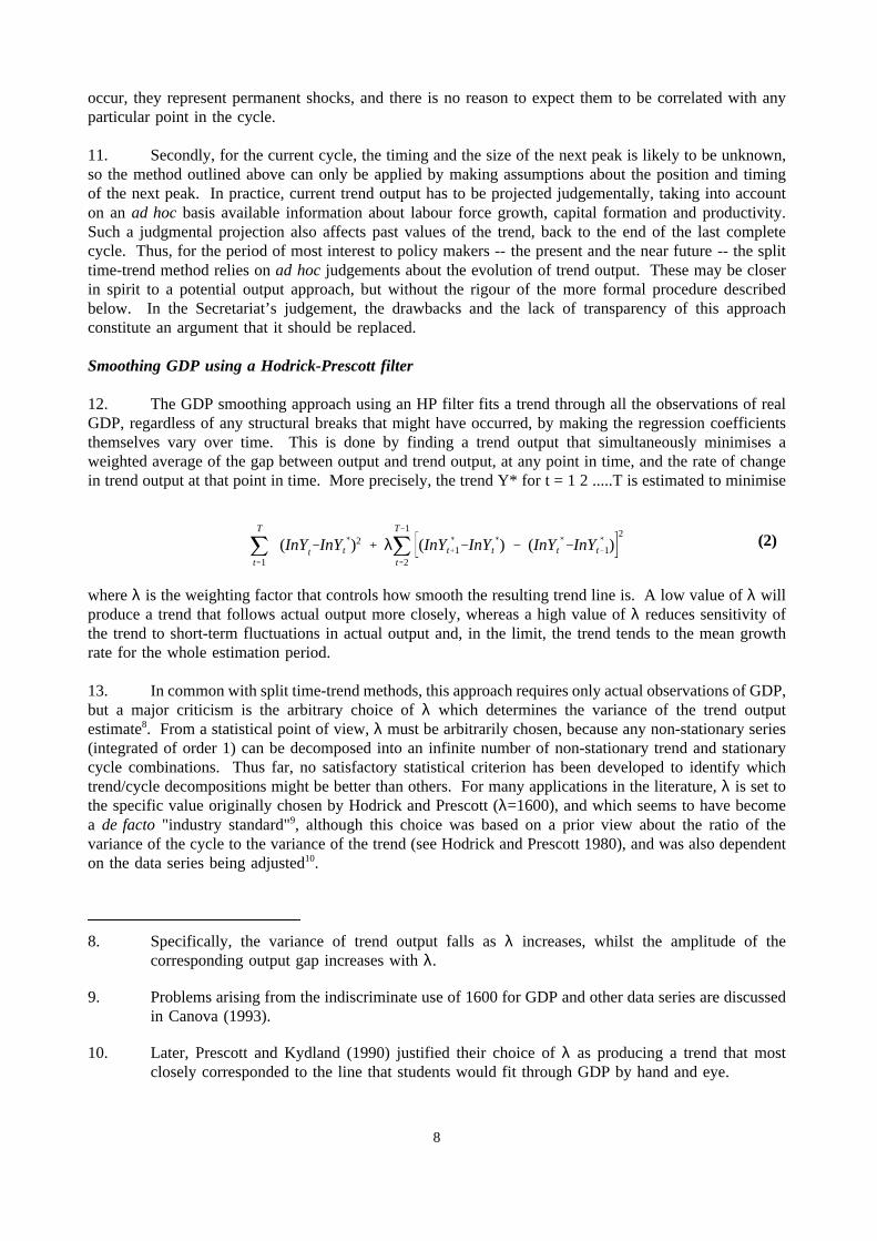
12. The GDP smoothing approach using an HP filter fits a trend through all the observations of realGDP, regardless of any structural breaks that might have occurred, by making the regression coefficientsthemselves vary over time. This is done by finding a trend output that simultaneously minimises aweighted average of the gap between output and trend output, at any point in time, and the rate of changein trend output at that point in time. More precisely, the trend Y* fort = 1 2 .....T is estimated to minimise
whereλ is the weighting factor that controls how smooth the resulting trend line is. A low value ofλ will
(2)T
t 1
(InYt InYt )2 λT 1
t 2
(InYt 1 InYt ) (InYt InYt 1)2
produce a trend that follows actual output more closely, whereas a high value ofλ reduces sensitivity ofthe trend to short-term fluctuations in actual output and, in the limit, the trend tends to the mean growthrate for the whole estimation period.
13. In common with split time-trend methods, this approach requires only actual observations of GDP,but a major criticism is the arbitrary choice ofλ which determines the variance of the trend outputestimate8. From a statistical point of view,λ must be arbitrarily chosen, because any non-stationary series(integrated of order 1) can be decomposed into an infinite number of non-stationary trend and stationarycycle combinations. Thus far, no satisfactory statistical criterion has been developed to identify whichtrend/cycle decompositions might be better than others. For many applications in the literature,λ is set tothe specific value originally chosen by Hodrick and Prescott (λ=1600), and which seems to have becomea de facto"industry standard"9, although this choice was based on a prior view about the ratio of thevariance of the cycle to the variance of the trend (see Hodrick and Prescott 1980), and was also dependenton the data series being adjusted10.
8. Specifically, the variance of trend output falls asλ increases, whilst the amplitude of thecorresponding output gap increases withλ.
9. Problems arising from the indiscriminate use of 1600 for GDP and other data series are discussedin Canova (1993).
10. Later, Prescott and Kydland (1990) justified their choice ofλ as producing a trend that mostclosely corresponded to the line that students would fit through GDP by hand and eye.
8
14. Since the choice ofλ remains a key judgement, there are three possible decision criteria. The firstwould be to follow Hodrick and Prescott’s approach and choose a constant ratio of the variances of trendoutput and actual output. This approach would generate a differentλ value for each country and wouldmean that countries whose actual output fluctuates more would also show greater fluctuation in trend. Asecond approach would be to impose a uniform degree of smoothness and the same variance in trend outputfor each country. However, the difficulty with both these criteria is that they ignore the possibility thatsome countries respond with greater flexibility to economic shocks than others. This would affect howclosely trend output would follow actual output.
15. A third approach is to choose a value ofλ that generates a pattern of cycles which is broadlyconsistent with prior views about past cycles in each country. Such a criteria is judgemental and is ableto incorporate (limited) information about the past, but it is also less transparent than the other criteria.This method generally leads to the choice of values ofλ which are small and relatively uniform acrosscountries11.
16. As with the split time-trend method, the HP filter method also has an end-point problem. In partthis reflects the fitting of a trend line symmetrically through the data: if the beginning and the end of thedata set do not reflect similar points in the cycle, then the trend will be pulled upwards or downwardstowards the path of actual output for the first few and the last few observations. For example, for thosecountries which are slower to emerge from recession, an HP filter will tend to underestimate trend outputgrowth for the current period. This problem can be reduced by using projections which go beyond theshort-term to the end of the current cycle. For example, in the current study, GDP projections from themost recent OECD medium-term reference scenario have been used to extend the period of estimation until2000 to give more stability to estimates for the current and short-term projections period. In effect thisamounts to giving specific weight to judgements about potential and output gaps embodied in thoseprojections, with HP filter estimates tending towards potential, provided the output gap is closed by the endof the extended sample period.
17. A further possible weakness of the method is the treatment of structural breaks, which aretypically smoothed over by the HP filter: moderating the break when it occurs, but spreading its effect outover several years, depending on the value ofλ. This may not be inappropriate if the break occursgradually over time but is problematic in the case of large discrete changes in output levels.
2. Estimating potential output
18. From the point of view of macroeconomic analysis, the most important limitation of both theabove smoothing methods is that they are largely mechanistic and bring to bear no information about thestructural constraints and limitations on production through the availability of factors of production or otherendogenous influences. Thus, trend output growth projected by time-series methods may be inconsistent(too high or too low) with what is known or being assumed about the growth in capital, labour supply orfactor productivity or may be unsustainable because of inflationary pressures. The preferred "potentialoutput" approach attempts to overcome these shortcomings whilst adjusting also for the limiting influenceof demand pressure on employment and inflation. It does so in a structural framework; one in whichconsistent judgement can also be exercised on some of the key elements.
11. In the present study a value ofλ = 25 was used for most OECD Member countries.
9
Decomposition of Growth in PotentialOutput
Growth inpotential output
Growth inbusiness sector
Growth in generalgovernment sector
Growth in potentialemployment
Growth in trend hoursworked
Growth in stock ofcapital
Growth in trend totalfactor productivity
Contribution of trendlabour productivity
Contribution of trendcapital productivity
Growth in working-agepopulation (adjusted for
government employment)
Growth in the trendparticipation rate
Effects of variations inNAWRU
10
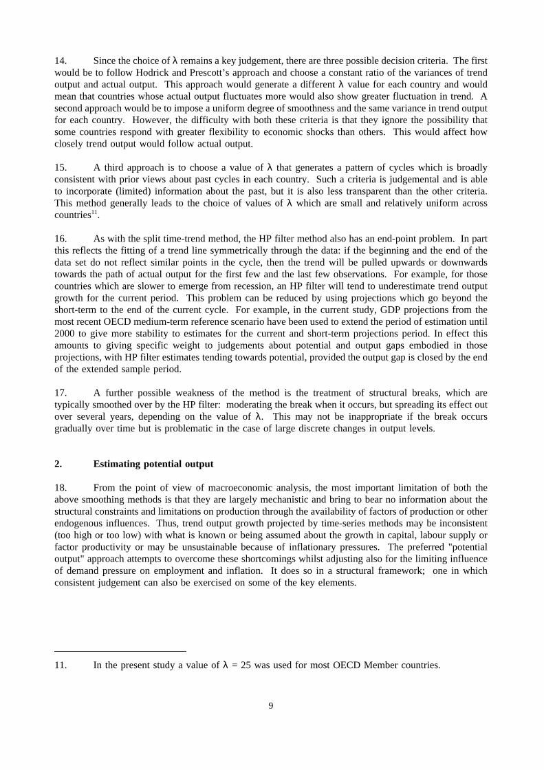
19. The framework of the OECD Secretariat’s analysis of potential output is broadly that adopted inits supply modelling work, as previously described by Torres and Martin (1989) and Torreset al. (1989).In its simplest form, a two-factor Cobb-Douglas production function for the business sector is estimatedfor each country, for given sample average labour shares. The estimated residuals from these equations arethen smoothed to give measures of trend total factor productivity. Potential output for the business sectoris then calculated by combining this measure of trend factor productivity with the actual capital stock andestimates of "potential" employment, using the same estimated production function. The chosen measureof "potential" employment is defined as the level of labour resources that might be employed withoutresulting in additional inflation. In effect, this amounts to adjusting the actual labour input used in theestimated production function for the gap between actual unemployment and the estimated NAWRU level.More specifically, the estimation method follows the following steps:
The estimated business-sector production function is assumed to be of the form:
LnY = LnA + αLnN + (1-α)LnK + LnE
i.e. y = a +αn + (1-α)k + e
where: Y = business-sector value addedN = actual business-sector labour inputK = actual business-sector capital input (excluding housing)E = total factor productivityα = average labour share parameterlower-case letters indicate natural logarithms.
20. For a given value of the labour share,α, the e series is calculated and then smoothed using aHodrick-Prescott filter to provide a measure of trend factor productivity, e*. Next, the trend factorproductivity series, e*, is substituted back into the production function along with actual capital stock, k,and "potential" employment, n*, to provide a measure of the log of business-sector potential, y*, as:
y* = a + αn* + (1-α)k + e*
where the level of potential employment in the business sector, N*, is then calculated as:
N* = LFS (1 - NAWRU) - EG
where: LFS = smoothed labour force (the product of the working age population and thetrend participation rate)
NAWRU = estimated non-accelerating wage rate of unemploymentEG = employment in the government sector.
21. The identification of appropriate measures of the NAWRU draws on a number of different sourcesof information. As the starting point, a set of estimates is derived using the method described by Elmeskov(1993) and Elmeskov and MacFarlan (1993). This method essentially assumes that the change in wageinflation is proportional to the gap between actual unemployment and the NAWRU. Assuming also thatthe NAWRU changes only gradually over time, successive observations on the changes in inflation andactual unemployment rates can then be used to calculate a time series corresponding to the implicit valueof the NAWRU. More specifically, it is assumed that the rate of change of wage inflation is proportionalto the gap between actual unemployment and the NAWRU, thus:
D2logW = -a(U - NAWRU) a>0
11
where D is the first-difference operator and W and U are the levels of wages and unemployment,respectively. Assuming the NAWRU to be constant between any two consecutive time periods, an estimateof a can be calculated as:
a = -D3logW/DU
which, in turn, is used to give the estimated NAWRU as:
NAWRU = U - (DU/D3logW)*D2logW
22. The resulting series are then smoothed to eliminate erratic movements12. As illustrated byElmeskov (op. cit.), such measures of the NAWRU come close to the results of comparable methods whichuse alternative Okun or Beveridge curve relationships as a starting point. For a number of major countries,this information was then supplemented by estimates based on recent wage equation estimates embeddedin the supply blocks of the INTERLINK model (see Turneret al., 1993), along with a range of previousestimates. The broad set of NAWRU estimates were then cross-checked by OECD Secretariat countryexperts and modified where additional country information was available.
23. Potential output for the whole economy is finally obtained by adding actual value added in thegovernment sector to business-sector potential output. Thus, for want of a superior alternative measure,actual value added in the government sector is taken to be equal to potential output in that sector. Thecalculation of potential output growth and the decomposition into its various components is illustratedschematically in the Box, and the decomposition into main components is provided in Table 1.
24. For Japan, a slightly different approach is used from the one outlined above. In particular, themost recent Secretariat estimates of the business sector production function for Japan (see Turneret al.,op. cit.) suggest that the Cobb-Douglas production function is inappropriate and instead a CES productionfunction is used, one with an estimated elasticity of substitution between capital and labour of 0.4. In thiscase, the decomposition of potential output growth into its component parts is more complex than shownabove.
3. Comparison of results
25. A general comparison of growth rates and output gaps for each country of estimated potentialoutput with previous split time-trend estimates and HP trend estimates is provided in Table 2 and Figure 1.There are several general features to note. Firstly, the symmetry properties are different. The calculationof trend output using a split time-trend or HP filter imposes the property that the output gaps are symmetricover the full estimation period (i.e. they sum to zero), even if the economy is not at the same point in thecycle at the beginning and the end of the period13. In contrast, such symmetry is not imposed on themeasures of potential but will depend on the relative positions of actual and NAWRU rates ofunemployment -- in particular the potential measure will only be exactly symmetric if the NAWRU estimateis exactly equal to average unemployment over the cycle.
12. To the extent that wage inflation is affected, not only by the level of unemployment but also itsyear-to-year changes, the derived short-run indicator will tend to move with actual unemploymentand may thus differ from the long-run NAWRU obtained for a constant rate of unemployment.
13. In fact, since the HP filter is applied to lnGDP, the resulting output gaps calculated from GDPand trend GDP are not quite symmetric. The asymmetry grows asλ rises, but for the chosenvalues ofλ presented here, this asymmetry is negligible.
12
26. Another important feature is that potential output growth rates may fluctuate from year to year,more so than trend growth rates derived from output smoothing. Using the decomposition of contributionsto potential growth shown in Table 1, the non-cyclical factors contributing to such variability are seen tovary from country to country. The three most important factors are variations in the NAWRU, the growthof capital stock and working-age population.
27. Since the NAWRU assumptions are necessarily imprecise and subject to a range of measurementproblems it is useful to provide some sensitivity analysis for the resulting estimates of potential output andoutput gaps. In practice, the consequences of choosing a higher or lower NAWRU estimate on theestimated level of potential output are quite straightforward and are inversely related to the "labour share"of business sector output. Thus for the United States, with an average labour share of 68 per cent,assuming a NAWRU estimate which is 1/2 per cent lower would raise the level of business sector potentialoutput by 0.3 to 0.4 per cent, implying a corresponding level shift in the estimate of the gap between actualand potential GDP. Since this entails a shift in the level of potential GDP, the consequences for theaverage growth rate of potential output are negligible or zero. Since the average labour shares of otherOECD countries typically vary between 65 to 75 per cent, their sensitivity to variations in NAWRUestimates are broadly similar to the United States case.
28. Comparing across output gap estimates in Figure 1, the main turning points and broadcharacteristics are seen, with some exceptions, to be broadly consistent for each country, though this is alsoa reflection of the major peaks and troughs in the growth of actual GDP. Over the sample period up tothe start of the recent recession, the broad developments shown for most countries are highly correlatedacross measures, though with varying degrees of differences. In general, the HP filter-based measures tendto suggest cycles of slightly lesser amplitude and hence smaller output gaps than either potential or splittime trend measures, reflecting the specific values of theλ parameter used in the calculation. For mostcountries however, these differences do not seem to be large.
29. There are however a number of exceptions -- most notably for Austria, Finland, Japan, Norwayand Spain -- where one or other measure behaves differently over some part of the sample. For thepotential measure, the factors responsible can be readily identified with specific information andassumptions about non-cyclical or discrete changes in supply factors -- shifts in working hours, capitalstock, participation rates, working population and/or the NAWRU estimates (as reported in Table 1). Forthe time series measures, these factors are not taken into account and the trend estimates simply reflectdevelopments in GDP over time, given the chosen values of the smoothing parameter or the dating of thepeaks, depending on the method used.
30. Over the period of more immediate concern, -- the recent past, the present and the projectionperiod -- there is clearer evidence of systematic differences, reflecting the inherent problems in projectingthe split time trend through to the end of the current cycle. Most noticeably, for Canada, France, Italy andJapan, the split time trend measures give much larger estimates of the output gap than either potential orthe HP filter for the current projection period. Moreover in each of these cases the measures given bypotential and HP methods are much closer over the recent past.
31. These results underscore the need for consistent judgement and hence a framework of assessmentin which the behavioural assumptions underlying the projection can be clearly identified and, as necessary,challenged and adjusted according to new information i.e. a process which goes beyond the mechanicalapplication of time series methods to GDP. The latter are nonetheless useful where significant deviationsof the potential estimates from a suitably calibrated trend may signal the need for a closer examination ofthe underlying macroeconomic and structural assumptions being made -- either about the estimate ofpotential or the medium-term projections. For these reasons, the preferred approach is to use the potential
13
measure, subject to its plausibility being checked against a suitably selected time series estimate oftrend GDP.
III. Estimating Structural Budget Balances
32. The overall purpose of adjusting government balances for changes in economic activity is to geta clearer picture of the underlying fiscal situation and to use this as a guide to fiscal policy analysis. Thestructural budget balance reflects what government revenues and expenditures would be if output was atits potential level and therefore does not reflect cyclical developments in economic activity. In contrast,the actual budget balance does reflect the cyclical component of economic activity and therefore fluctuatesaround the structural budget balance. In practice, the structural budget balance must be estimated by takingactual government revenues and expenditures and breaking them into an estimated cyclical component andan estimated structural component. More precisely, the structural budget balance measures what the balanceof tax revenues less government expenditure would be if actual GDP corresponded to potential GDP. Thus:
B* = ∑Ti* - G* + capital spending
where: B* = structural budget balanceTi* = structural tax revenues for the ith category of taxG* = structural government expenditures (excluding capital spending)
33. In practice, the components of the structural budget balance must be estimated from actual taxrevenues (broken into four categories: corporate tax, income tax, social security contributions, and indirecttaxes) and government expenditures using the property that each component of the budget is adjustedproportionately to the ratio of potential output to actual output, as determined by its elasticity. Thus:
where: Ti = actual tax revenues for the ith category of taxG = actual government expenditures (excluding capital spending)Y = level of actual outputY* = level of potential outputαi = elasticity of ith tax category with respect to outputβ = elasticity of current government expenditures with respect to output
From these relationships, the structural budget balance can be derived as follows:
34. The split between estimated cyclical and structural components is relatively sensitive to theestimated output gaps. Typically, if the estimated output gap were 1 percentage point of GDP smaller, theestimated structural component of the actual budget balance would be larger by around 1/2 percentage point
14

of GDP. Estimates of the impact of economic activity on budget balances also indicate that tax revenueadjustments far outweigh the effect of expenditure adjustments, which make up only about 10 to 20 per centof the adjustment. This is because almost all taxes are affected by economic fluctuation, whereas a muchsmaller proportion of expenditure is devoted to dealing with unemployment and of that, only a portion iscyclical.
1. Tax elasticities
35. The Secretariat method makes adjustments to four separate categories of taxes in calculatingstructural budget balances: corporate taxes, personal income taxes, social security contributions (employersand employees), and indirect taxes. The tax elasticities previously used by the Secretariat have beenderived from various sources and while some have been updated on anad hocbasis over the years, someare now out of date, because of tax reforms that have taken place.
36. One approach would be to calculate elasticities using a simple regression of taxes on output (incurrent prices). The results of this approach, estimated using data from 1960 to 1992 are shown in Table 3.However, these regressions show the average elasticity over the whole period rather than the currentelasticity and embody policy changes in addition to "automatic" effects.
37. For household income tax and social security contributions, new elasticities have been estimated,drawing on data available from various parts of the Secretariat. Average and marginal income tax andsocial security contribution rates applying to each level of income (and different family circumstance) havebeen compiled on a systematic basis by the Fiscal Affairs Division of the OECD Secretariat. Weightedaverages of these average and marginal tax rates have been calculated using weights derived from incomedistributions estimated from data provided in the Employment Outlook. The ratio between marginal taxand average tax provides the elasticity with respect to gross earnings. This elasticity is then converted toa GDP elasticity, allowing for cross-country variation in the responsiveness of employment and wages tofluctuations in real output (see Annex 1 for details). The new personal income tax elasticities show muchgreater variability across countries, while the new social security elasticities are generally higher than theprevious elasticities.
38. For corporate taxes and indirect taxes, it has proved more difficult to find reliable alternativemethods for estimating them. For corporate taxes, it has been decided to maintain the existing elasticitiesin the meantime, even though these elasticities do not incorporate up-to-date information on currentcorporate-tax regimes. For indirect taxes, the previously used elasticities that were used were also quiteout of date and it was considered that an assumption of unit elasticity was more appropriate than continuingto the earlier ones. The set of elasticities previously used and the new set of elasticities are shown inTable 4.
2. Expenditure elasticities
39. Until now, the adjustment of expenditure for the effects of the cycle has used an average elasticityof -0.2 for all countries, estimated using the Okun elasticities method described below, for lack of additionaldata. New expenditure elasticities have been estimated for each country, based on the elasticity of theunemployment rate with respect to output (which is the reciprocal of the Okun coefficient), multiplied bythe elasticity of unemployment benefits with respect to unemployment. This provides an elasticity ofunemployment benefits with respect to output, that can then be applied to all current governmentexpenditure as shown in Table 5. While it would be preferable to adjust unemployment benefit expendituredirectly (and any other cyclical components of government expenditure), up-to-date data on unemployment
15

benefit expenditure are not readily available. In any case, even with significant increases in unemployment,these expenditures remain a small part of total government expenditures, as shown in Table 6.
3. Structural budget balances: results
40. Adjusted budget balances calculated using the previous (split time trend) method, and the new(potential output) method are presented in Table 7 and shown in Figure 2, using the previous and therevised tax and expenditure elasticities. As noted above, it is clear that the revision of elasticities does notplay a major role in explaining the differences in structural budget balances, compared with structuralbalances previously published by the Secretariat. Instead, where there are major differences, these largelymirror the revision in output gaps.
41. Structural deficits for almost all countries except the United States have been revised significantly.Among the seven major countries, Germany and the United Kingdom’s structural deficit positions now lookbetter than previously projected, reflecting larger negative output gaps than under the previous method.For Japan, France, Italy and Canada, structural deficits are significantly larger than previously estimated.For Italy, between 1993 and 1996 the structural deficit, as calculated using the new method, is on average2 percentage points larger than with the previous method. Taking the period from 1993 to 1996, the pathof consolidation also shows some differences for some countries (see Table 8). During that period, Japanis projected to have eased its fiscal stance by more than was estimated using the previous method, and withthe new method, France, Italy and Canada are projected to achieve less consolidation than previouslyestimated.
42. Among the smaller countries, structural deficits for Belgium, Finland, Ireland and the Netherlandsare projected to be significantly smaller than under the previous method. For all these countries, outputgaps are larger than previously estimated. For Finland, the previous method showed a deterioratingstructural deficit position between 1993 and 1996, whereas the new method indicates some consolidation.Spain on the other hand, is now estimated to achieve less consolidation than projected using the previousmethod.
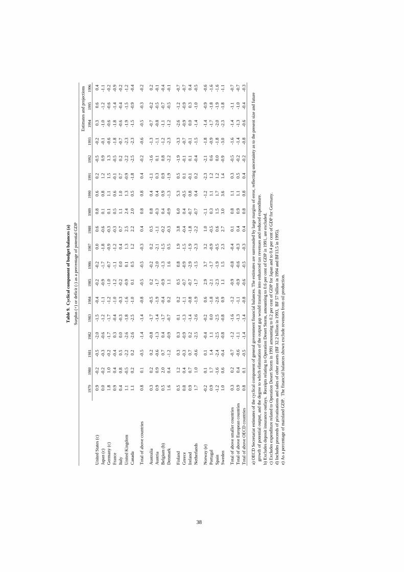
43. In general, the cyclical part of budget balances, calculated with the new (potential output) method,should tend to balance out over time as accumulations of debt due to cyclical deficits should be offset bycyclical surpluses although this will depend on the symmetry properties of the output gap measure, asdiscussed earlier. Therefore, it would also be possible for cyclical deficits or surpluses to persist for quitelong periods of time. The cyclical component of budget balances (as a per cent of potential GDP)calculated with the new method and the new set of elasticities is shown in Table 9.
IV. Conclusions
44. The analysis presented in this paper suggests that the Secretariat’s previous method used formeasuring the output gap by applying split time trend analysis to GDP -- and using it as an input to theconstruction of its structural budget balances -- was subject to a number of serious shortcomings. Inparticular it took little or no account of the actual timing of changes in structural factors that affectproductive potential and was difficult to estimate and project for the current period and the near futurewhich are most relevant for policy making.
16

45. A review of the strengths and weaknesses of alternative methods suggests that a consistentapproach should be used for both conjunctural and fiscal assessments, one which is behavioural andrepresents a potential rate of growth which is sustainable at a stable rate of inflation. The preferred measureis therefore one based on a production function approach and which takes explicit account of structuralinformation, in particular with respect to the NAWRU and the "speed-limits" to growth.
46. Although it is recognised that all output gap measures are subject to considerable uncertainty, akey result arising from the comparisons of the measures considered is that the Secretariat’s previous splittime trend measure has tended to overestimate the output gaps for the present and immediate future forsome countries and underestimate the gaps for others. This has important consequences for the assessmentof fiscal positions. The resulting estimated structural budget balances must, however, be interpreted withgreat caution as they are surrounded by a considerable margin of uncertainty, particularly in economiesundergoing substantial restructuring.
17

Data up to end-1990 are for western Germany only; unless otherwise indicated, they are for thewhole of Germany from 1991 onwards. In tables showing percentage changes from the previousyear, data refer to the whole of Germany from 1992 onwards.
18

Table 1. Contributions to growth in business sector potential output and NAWRUs
Business sectorpotential output
Employmentcontribution
Trend hoursCapital
contributionTrend TFP NAWRU
Actualunemployment
United States1986 2.9 1.4 -0.1 1.0 0.6 6.2 7.01987 2.6 1.2 -0.1 0.9 0.6 5.9 6.21988 2.4 1.0 0.0 0.9 0.6 5.7 5.51989 2.0 0.5 0.0 0.9 0.6 5.8 5.31990 1.9 0.5 0.0 0.8 0.6 5.8 5.51991 2.4 1.0 0.1 0.7 0.6 5.8 6.71992 2.3 0.9 0.1 0.6 0.7 6.0 7.41993 2.4 0.9 0.1 0.7 0.7 6.1 6.81994 2.7 0.9 0.1 0.9 0.7 6.2 6.11995 2.8 0.8 0.1 1.0 0.8 6.2 5.61996 2.7 0.8 0.1 1.1 0.8 6.2 5.6
Germany (Western)1986 1.8 -0.1 -0.5 0.8 1.6 7.3 7.71987 2.1 0.0 -0.5 0.8 1.7 7.3 7.61988 2.6 0.4 -0.5 0.9 1.8 7.2 7.61989 3.1 0.8 -0.5 0.9 1.9 7.0 6.91990 3.9 1.4 -0.5 1.0 1.9 6.9 6.21991 3.5 0.9 -0.5 1.2 1.9 6.8 5.51992 3.4 0.9 -0.5 1.1 1.8 6.9 5.81993 2.7 0.5 -0.4 0.8 1.7 7.0 7.31994 2.5 0.4 -0.4 0.7 1.7 7.1 8.21995 2.4 0.3 -0.4 0.7 1.7 7.2 7.91996 2.4 0.2 -0.4 0.8 1.7 7.3 7.5
France1986 2.3 -0.1 0.0 0.8 1.7 8.9 10.41987 2.7 0.2 0.0 0.8 1.6 9.0 10.51988 2.9 0.3 0.0 0.9 1.6 9.0 10.01989 3.0 0.4 0.0 1.0 1.5 9.0 9.41990 2.7 0.1 0.0 1.1 1.5 9.1 8.91991 2.4 0.0 0.0 1.0 1.4 9.1 9.51992 2.1 -0.2 0.0 0.9 1.4 9.2 10.41993 1.8 -0.3 0.0 0.7 1.4 9.2 11.71994 2.2 0.2 0.0 0.6 1.4 9.2 12.61995 2.3 0.3 0.0 0.6 1.4 9.2 12.31996 2.4 0.3 0.0 0.7 1.4 9.2 11.7
Italy1986 2.0 0.0 .. 0.7 1.3 10.4 11.21987 1.6 -0.5 .. 0.8 1.4 10.7 12.11988 2.7 0.4 .. 0.9 1.4 11.0 12.11989 1.9 -0.5 .. 0.9 1.4 11.0 12.11990 2.7 0.3 .. 1.0 1.4 11.0 11.51991 2.5 0.1 .. 0.9 1.5 11.0 11.01992 2.6 0.3 .. 0.8 1.5 10.8 11.61993 2.4 0.3 .. 0.5 1.6 10.5 10.41994 2.2 0.2 .. 0.4 1.7 10.2 11.31995 2.4 0.2 .. 0.4 1.7 9.8 11.21996 2.5 0.2 .. 0.5 1.8 9.5 11.0
19

Table 1. (Continued)
Business sectorpotential output
Employmentcontribution
Capitalcontribution
Trend TFP NAWRUActual
unemployment
United Kingdom1986 2.7 0.3 0.6 1.9 10.2 11.01987 2.8 0.3 0.6 1.8 9.8 9.81988 3.1 0.6 0.8 1.7 9.3 7.81989 3.5 0.9 0.9 1.6 8.8 6.11990 3.0 0.6 0.7 1.6 8.4 5.91991 3.5 1.4 0.4 1.6 8.2 8.21992 3.1 1.2 0.3 1.7 8.0 9.91993 2.3 0.3 0.2 1.7 7.8 10.21994 2.3 0.3 0.2 1.8 7.7 9.41995 2.5 0.4 0.3 1.8 7.6 8.71996 2.6 0.4 0.4 1.9 7.5 7.9
Canada1986 2.6 0.9 1.3 0.4 9.0 9.51987 2.4 0.8 1.4 0.3 9.0 8.81988 3.1 1.1 1.7 0.3 9.0 7.81989 3.1 1.1 1.8 0.2 9.0 7.51990 3.0 1.2 1.6 0.2 9.0 8.11991 2.6 1.0 1.4 0.2 8.8 10.31992 2.0 0.6 1.1 0.3 8.6 11.31993 1.8 0.5 0.9 0.4 8.5 11.21994 2.7 1.2 1.0 0.5 8.5 10.51995 2.9 1.3 1.1 0.5 8.5 9.71996 3.0 1.3 1.2 0.6 8.5 9.2
Australia1986 3.3 1.2 1.2 0.9 7.9 8.01987 3.5 1.4 1.2 0.9 7.9 8.01988 3.7 1.5 1.3 0.9 8.0 7.11989 4.3 1.9 1.5 0.9 8.1 6.11990 3.2 1.0 1.2 0.9 8.3 7.01991 2.8 1.0 0.8 0.9 8.1 9.51992 3.3 1.6 0.7 0.9 8.0 10.71993 2.9 1.3 0.6 1.0 7.9 10.91994 2.9 1.2 0.7 1.0 7.8 9.71995 3.2 1.3 0.9 1.0 7.7 8.71996 3.4 1.3 1.0 1.0 7.6 7.9
Austria1986 1.1 -0.8 1.1 0.9 3.4 3.11987 1.9 0.0 1.1 0.9 3.5 3.81988 1.9 -0.1 1.2 0.8 3.5 3.61989 2.0 0.0 1.2 0.8 3.5 3.11990 3.6 1.4 1.3 0.8 3.5 3.21991 2.8 0.7 1.3 0.8 3.5 3.51992 2.3 0.3 1.2 0.8 3.5 3.61993 2.3 0.5 1.0 0.8 3.7 4.21994 2.2 0.4 1.1 0.8 3.9 4.41995 2.4 0.5 1.1 0.8 4.0 4.21996 2.6 0.7 1.2 0.8 4.0 4.1
20
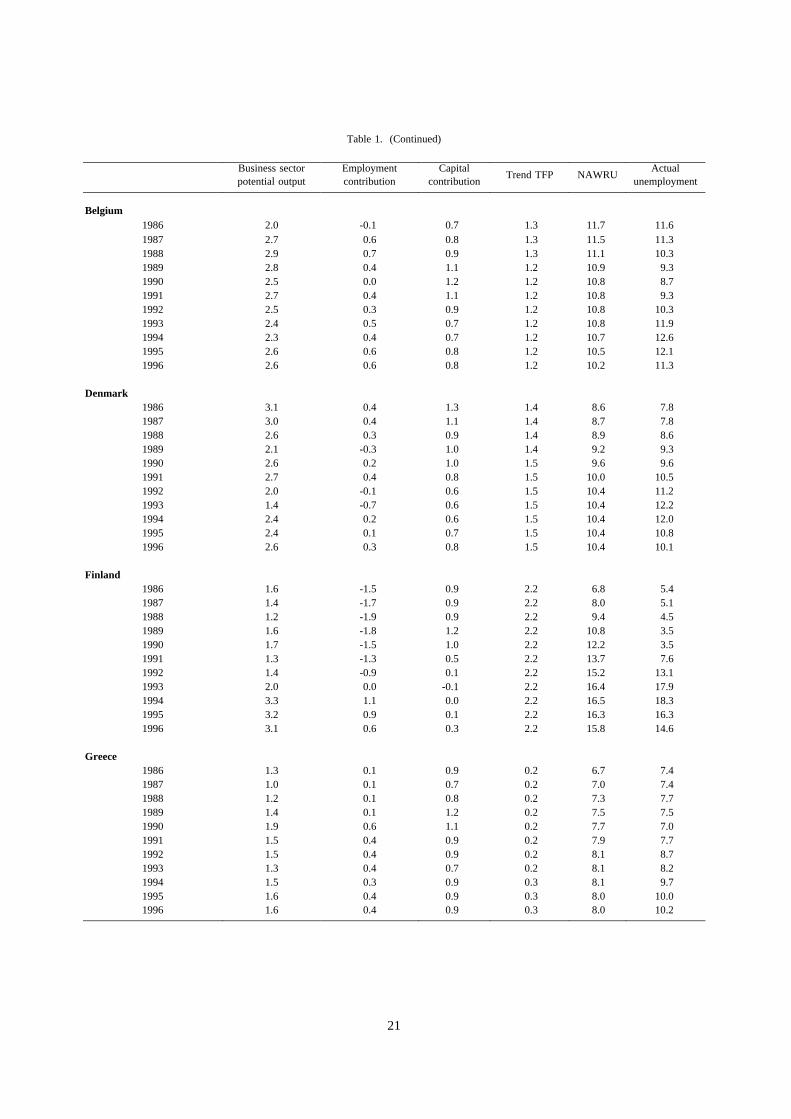
Table 1. (Continued)
Business sectorpotential output
Employmentcontribution
Capitalcontribution
Trend TFP NAWRUActual
unemployment
Belgium1986 2.0 -0.1 0.7 1.3 11.7 11.61987 2.7 0.6 0.8 1.3 11.5 11.31988 2.9 0.7 0.9 1.3 11.1 10.31989 2.8 0.4 1.1 1.2 10.9 9.31990 2.5 0.0 1.2 1.2 10.8 8.71991 2.7 0.4 1.1 1.2 10.8 9.31992 2.5 0.3 0.9 1.2 10.8 10.31993 2.4 0.5 0.7 1.2 10.8 11.91994 2.3 0.4 0.7 1.2 10.7 12.61995 2.6 0.6 0.8 1.2 10.5 12.11996 2.6 0.6 0.8 1.2 10.2 11.3
Denmark1986 3.1 0.4 1.3 1.4 8.6 7.81987 3.0 0.4 1.1 1.4 8.7 7.81988 2.6 0.3 0.9 1.4 8.9 8.61989 2.1 -0.3 1.0 1.4 9.2 9.31990 2.6 0.2 1.0 1.5 9.6 9.61991 2.7 0.4 0.8 1.5 10.0 10.51992 2.0 -0.1 0.6 1.5 10.4 11.21993 1.4 -0.7 0.6 1.5 10.4 12.21994 2.4 0.2 0.6 1.5 10.4 12.01995 2.4 0.1 0.7 1.5 10.4 10.81996 2.6 0.3 0.8 1.5 10.4 10.1
Finland1986 1.6 -1.5 0.9 2.2 6.8 5.41987 1.4 -1.7 0.9 2.2 8.0 5.11988 1.2 -1.9 0.9 2.2 9.4 4.51989 1.6 -1.8 1.2 2.2 10.8 3.51990 1.7 -1.5 1.0 2.2 12.2 3.51991 1.3 -1.3 0.5 2.2 13.7 7.61992 1.4 -0.9 0.1 2.2 15.2 13.11993 2.0 0.0 -0.1 2.2 16.4 17.91994 3.3 1.1 0.0 2.2 16.5 18.31995 3.2 0.9 0.1 2.2 16.3 16.31996 3.1 0.6 0.3 2.2 15.8 14.6
Greece1986 1.3 0.1 0.9 0.2 6.7 7.41987 1.0 0.1 0.7 0.2 7.0 7.41988 1.2 0.1 0.8 0.2 7.3 7.71989 1.4 0.1 1.2 0.2 7.5 7.51990 1.9 0.6 1.1 0.2 7.7 7.01991 1.5 0.4 0.9 0.2 7.9 7.71992 1.5 0.4 0.9 0.2 8.1 8.71993 1.3 0.4 0.7 0.2 8.1 8.21994 1.5 0.3 0.9 0.3 8.1 9.71995 1.6 0.4 0.9 0.3 8.0 10.01996 1.6 0.4 0.9 0.3 8.0 10.2
21

Table 1. (Continued)
Business sectorpotential output
Employmentcontribution
Capitalcontribution
Trend TFP NAWRUActual
unemployment
Ireland1986 3.3 -0.3 0.4 3.2 16.9 17.41987 3.9 0.2 0.5 3.2 17.4 17.51988 4.8 1.0 0.6 3.3 17.7 16.71989 6.1 2.1 0.7 3.3 17.2 15.61990 5.6 1.5 0.8 3.3 16.6 13.71991 5.0 1.1 0.6 3.3 16.1 15.71992 4.9 1.1 0.5 3.3 15.7 16.31993 4.6 0.9 0.4 3.3 15.4 16.71994 4.9 1.1 0.4 3.3 14.8 15.81995 4.4 0.5 0.5 3.3 14.8 15.31996 4.4 0.5 0.5 3.3 14.8 14.7
Netherlands1986 2.7 0.7 0.9 1.1 9.2 9.91987 2.6 0.7 0.8 1.1 9.3 9.61988 2.7 0.8 0.8 1.1 9.3 9.21989 2.6 0.6 0.9 1.1 9.3 8.31990 2.7 0.6 1.0 1.1 9.3 7.51991 2.8 0.7 1.0 1.1 9.3 7.01992 2.7 0.7 0.9 1.0 9.2 6.71993 2.4 0.6 0.8 1.0 9.1 8.31994 2.4 0.6 0.8 1.0 8.9 9.31995 2.5 0.6 0.8 1.0 8.7 8.61996 2.5 0.5 0.9 1.0 8.5 7.9
Norway (Mainland)1986 2.2 0.7 1.0 0.5 3.1 2.01987 1.8 0.4 0.9 0.5 3.3 2.11988 1.6 0.3 0.7 0.6 3.7 3.21989 0.5 -0.6 0.4 0.6 4.1 4.91990 0.2 -0.8 0.4 0.6 4.5 5.21991 0.4 -0.6 0.3 0.7 4.9 5.51992 0.8 -0.3 0.3 0.7 5.2 5.91993 1.2 0.1 0.3 0.8 5.3 6.01994 1.2 0.0 0.4 0.8 5.4 5.51995 2.0 0.7 0.4 0.8 5.3 5.21996 2.2 0.9 0.5 0.8 5.1 4.8
Spain1986 1.4 -0.8 0.7 1.5 19.1 21.01987 2.7 0.1 1.1 1.5 19.4 20.51988 3.1 0.3 1.3 1.5 19.5 19.51989 2.8 -0.3 1.6 1.5 19.6 17.31990 2.9 -0.2 1.6 1.5 19.8 16.31991 2.9 -0.1 1.5 1.5 20.0 16.31992 2.8 0.1 1.3 1.5 20.3 18.41993 2.3 0.0 0.8 1.5 20.7 22.71994 2.1 0.0 0.6 1.5 21.0 24.31995 3.0 0.9 0.7 1.5 20.5 24.01996 3.1 0.9 0.7 1.5 20.0 23.4
22
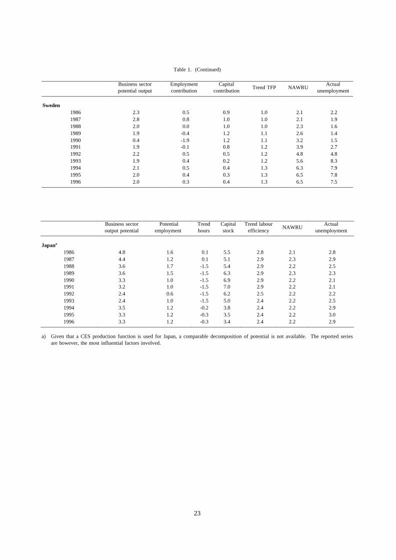
Table 1. (Continued)
Business sectorpotential output
Employmentcontribution
Capitalcontribution
Trend TFP NAWRUActual
unemployment
Sweden1986 2.3 0.5 0.9 1.0 2.1 2.21987 2.8 0.8 1.0 1.0 2.1 1.91988 2.0 0.0 1.0 1.0 2.3 1.61989 1.9 -0.4 1.2 1.1 2.6 1.41990 0.4 -1.9 1.2 1.1 3.2 1.51991 1.9 -0.1 0.8 1.2 3.9 2.71992 2.2 0.5 0.5 1.2 4.8 4.81993 1.9 0.4 0.2 1.2 5.6 8.31994 2.1 0.5 0.4 1.3 6.3 7.91995 2.0 0.4 0.3 1.3 6.5 7.81996 2.0 0.3 0.4 1.3 6.5 7.5
Business sectoroutput potential
Potentialemployment
Trendhours
Capitalstock
Trend labourefficiency
NAWRUActual
unemployment
Japana
1986 4.8 1.6 0.1 5.5 2.8 2.1 2.81987 4.4 1.2 0.1 5.1 2.9 2.3 2.91988 3.6 1.7 -1.5 5.4 2.9 2.2 2.51989 3.6 1.5 -1.5 6.3 2.9 2.3 2.31990 3.3 1.0 -1.5 6.9 2.9 2.2 2.11991 3.2 1.0 -1.5 7.0 2.9 2.2 2.11992 2.4 0.6 -1.5 6.2 2.5 2.2 2.21993 2.4 1.0 -1.5 5.0 2.4 2.2 2.51994 3.5 1.2 -0.2 3.8 2.4 2.2 2.91995 3.3 1.2 -0.3 3.5 2.4 2.2 3.01996 3.3 1.2 -0.3 3.4 2.4 2.2 2.9
a) Given that a CES production function is used for Japan, a comparable decomposition of potential is not available. The reported seriesare however, the most influential factors involved.
23
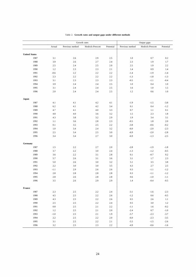
Table 2. Growth rates and output gaps under different methods
Growth rates Output gaps
Actual Previous method Hodrick-Prescott Potential Previous method Hodrick-Prescott Potential
United States
1987 3.1 2.6 2.9 2.5 1.0 0.7 0.2
1988 3.9 2.6 2.7 2.4 2.3 1.9 1.7
1989 2.5 2.4 2.5 2.0 2.5 1.9 2.2
1990 1.2 2.3 2.3 2.1 1.4 0.9 1.4
1991 -0.6 2.2 2.2 2.2 -1.4 -1.9 -1.4
1992 2.3 2.2 2.2 2.2 -1.3 -1.8 -1.3
1993 3.1 2.3 2.3 2.3 -0.5 -1.1 -0.4
1994 3.9 2.4 2.4 2.5 1.0 0.4 1.0
1995 3.1 2.4 2.4 2.5 1.6 1.0 1.5
1996 2.0 2.4 2.4 2.5 1.2 0.6 1.0
Japan
1987 4.1 4.1 4.2 4.1 -1.9 -1.5 -3.8
1988 6.2 4.1 4.2 3.4 0.1 0.4 -1.2
1989 4.7 4.1 4.0 3.3 0.7 1.1 0.1
1990 4.8 4.0 3.6 3.2 1.5 2.3 1.8
1991 4.3 3.8 3.2 2.9 1.9 3.4 3.1
1992 1.1 3.6 2.8 2.3 -0.5 1.8 2.0
1993 0.1 3.5 2.5 2.2 -3.8 -0.6 -0.2
1994 1.0 3.4 2.4 3.2 -6.0 -2.0 -2.3
1995 2.5 3.4 2.5 3.0 -6.9 -2.0 -2.8
1996 3.4 3.4 2.7 3.0 -6.9 -1.3 -2.5
Germany
1987 1.5 2.2 2.7 2.0 -2.8 -1.9 -1.8
1988 3.7 2.2 3.0 2.4 -1.3 -1.2 -0.5
1989 3.6 2.2 3.1 2.8 0.1 -0.7 0.2
1990 5.7 2.6 3.1 3.6 3.1 1.7 2.3
1991 5.0 2.6 3.0 3.2 5.1 3.5 3.8
1992 2.2 3.0 3.0 3.5 4.3 2.7 2.5
1993 -1.1 2.9 2.6 2.6 0.3 -1.1 -1.2
1994 2.8 2.8 2.8 2.8 0.3 -1.1 -1.2
1995 2.8 2.6 2.8 2.8 0.6 -1.0 -1.1
1996 3.5 2.6 2.9 2.9 1.4 -0.4 -0.5
France
1987 2.3 2.5 2.2 2.4 -3.1 -1.6 -2.3
1988 4.5 2.5 2.2 2.6 -1.2 0.6 -0.5
1989 4.3 2.5 2.2 2.6 0.5 2.6 1.1
1990 2.5 2.5 2.2 2.4 0.5 3.0 1.2
1991 0.8 2.5 2.1 2.2 -1.1 1.6 -0.2
1992 1.2 2.5 2.1 2.0 -2.4 0.7 -1.0
1993 -1.0 2.5 2.1 1.9 -5.7 -2.3 -3.7
1994 2.2 2.5 2.2 2.0 -6.0 -2.3 -3.5
1995 3.1 2.5 2.2 2.1 -5.5 -1.5 -2.6
1996 3.2 2.5 2.3 2.2 -4.9 -0.6 -1.6
24

Table 2 (continued)
Growth rates Output gaps
Actual Previous method Hodrick-Prescott Potential Previous method Hodrick-Prescott Potential
Italy
1987 3.1 2.4 2.5 1.7 -1.0 -0.3 1.5
1988 4.1 2.4 2.5 2.6 0.6 1.2 2.9
1989 2.9 2.4 2.3 1.8 1.2 1.8 4.0
1990 2.1 2.4 2.1 2.5 0.9 1.9 3.7
1991 1.2 2.4 1.8 2.3 -0.3 1.3 2.6
1992 0.7 2.4 1.7 2.5 -1.9 0.3 0.8
1993 -0.7 2.4 1.7 2.3 -4.8 -2.0 -2.1
1994 2.2 2.4 1.8 2.1 -5.0 -1.7 -2.0
1995 2.7 2.4 2.0 2.0 -4.8 -1.0 -1.4
1996 2.9 2.4 2.2 2.2 -4.3 -0.4 -0.7
United Kingdom
1987 4.8 2.6 2.5 2.5 3.0 2.6 2.8
1988 5.0 2.6 2.4 2.8 5.5 5.2 5.0
1989 2.2 2.6 2.3 2.7 5.1 5.1 4.6
1990 0.4 2.6 2.1 2.7 2.9 3.3 2.2
1991 -2.0 2.3 2.0 2.8 -1.3 -0.7 -2.5
1992 -0.5 2.3 2.0 2.3 -4.0 -3.2 -5.1
1993 2.0 2.3 2.1 2.1 -4.2 -3.2 -5.2
1994 3.5 2.3 2.2 2.1 -3.0 -2.0 -3.9
1995 3.4 2.3 2.3 2.3 -1.9 -1.0 -2.9
1996 3.0 2.3 2.4 2.4 -1.2 -0.4 -2.3
Canada
1987 4.2 3.0 2.7 2.6 1.3 2.2 2.6
1988 5.0 3.0 2.6 3.0 3.3 4.6 4.6
1989 2.4 3.0 2.5 3.0 2.7 4.6 4.0
1990 -0.2 2.7 2.4 2.9 -0.2 1.9 0.8
1991 -1.8 2.5 2.4 2.6 -4.5 -2.3 -3.5
1992 0.6 2.5 2.4 2.0 -6.2 -4.0 -4.8
1993 2.2 2.5 2.5 1.8 -6.5 -4.3 -4.4
1994 4.1 2.7 2.6 2.5 -5.2 -2.8 -2.9
1995 4.2 3.0 2.7 2.9 -4.2 -1.4 -1.7
1996 3.9 3.0 2.8 3.0 -3.3 -0.3 -0.8
Australia
1987 4.7 4.1 3.4 3.4 0.7 0.9 0.6
1988 4.1 4.1 3.2 3.4 0.7 1.7 1.3
1989 4.5 4.1 3.0 3.6 1.1 3.3 2.2
1990 1.3 2.7 2.7 3.1 -0.3 1.9 0.4
1991 -1.3 2.7 2.6 2.7 -4.2 -2.0 -3.4
1992 2.1 2.7 2.7 2.8 -4.8 -2.6 -4.1
1993 3.8 2.7 2.9 2.5 -3.9 -1.7 -2.9
1994 4.3 2.7 3.1 2.8 -2.4 -0.6 -1.4
1995 4.3 2.7 3.3 3.0 -1.0 0.3 -0.2
1996 4.0 2.7 3.4 3.1 0.2 0.8 0.6
25

Table 2 (continued)
Growth rates Output gaps
Actual Previous method Hodrick-Prescott Potential Previous method Hodrick-Prescott Potential
Austria
1987 1.7 2.2 2.4 1.9 -2.3 -2.0 -4.3
1988 4.1 2.2 2.6 1.9 -0.6 -0.6 -2.3
1989 3.8 3.0 2.7 2.0 0.2 0.5 -0.5
1990 4.2 3.0 2.7 2.9 1.4 2.0 0.8
1991 2.7 3.0 2.6 2.8 1.2 2.1 0.7
1992 1.6 3.0 2.5 2.2 -0.2 1.2 0.1
1993 -0.3 2.2 2.4 2.1 -2.6 -1.4 -2.2
1994 2.6 2.2 2.4 2.1 -2.2 -1.2 -1.7
1995 3.0 2.2 2.5 2.2 -1.5 -0.6 -0.9
1996 3.1 2.2 2.5 2.4 -0.16 -0.1 -0.3
Belgium
1987 2.0 2.0 2.3 2.2 -2.7 -1.9 -2.5
1988 4.9 2.0 2.5 2.6 0.1 0.3 -0.4
1989 3.5 2.0 2.6 2.4 1.6 1.2 0.7
1990 3.2 2.0 2.5 2.3 2.8 2.0 1.6
1991 2.3 2.0 2.3 2.2 3.1 2.0 1.7
1992 1.9 2.0 2.1 2.1 3.0 1.7 1.5
1993 -1.7 2.0 2.0 2.1 -0.7 -1.9 -2.3
1994 2.3 2.0 2.0 2.1 -0.4 -1.7 -2.1
1995 3.0 2.0 2.1 2.3 0.7 -0.8 -1.3
1996 3.1 2.0 2.3 2.4 1.8 0.0 -0.7
Denmark
1987 0.3 2.0 2.0 2.6 0.9 1.4 0.7
1988 1.2 2.0 1.7 2.5 0.0 0.9 -0.6
1989 0.6 2.0 1.6 1.7 -1.4 -0.2 -1.7
1990 1.4 2.0 1.6 2.2 -1.9 -0.3 -2.5
1991 1.0 2.0 1.7 2.2 -2.9 -1.0 -3.6
1992 1.2 2.0 1.9 1.8 -3.6 -1.6 -4.1
1993 1.4 2.0 2.1 1.5 -4.1 -2.3 -4.2
1994 4.7 2.0 2.4 2.3 -1.6 0.0 -1.9
1995 3.3 2.0 2.6 2.1 -0.3 0.6 -0.8
1996 2.9 2.0 2.7 2.2 -0.6 0.8 -0.1
Finland
1987 4.1 2.5 2.6 1.7 3.4 0.2 4.0
1988 4.9 2.3 2.0 1.4 6.0 3.0 7.6
1989 5.7 2.0 1.3 1.6 9.9 7.4 11.9
1990 0.0 0.9 0.5 1.7 8.9 6.9 10.0
1991 -7.1 0.9 0.0 1.3 0.3 -0.6 0.9
1992 -3.6 0.9 -0.1 0.8 -4.2 -4.2 -3.5
1993 -2.0 0.9 0.3 0.9 -7.0 -6.4 -6.3
1994 3.5 0.9 1.1 2.1 -4.5 -4.1 -5.0
1995 4.8 0.9 1.8 2.2 -0.8 -1.3 -2.5
1996 3.9 0.9 2.5 2.6 2.1 0.1 -1.3
26
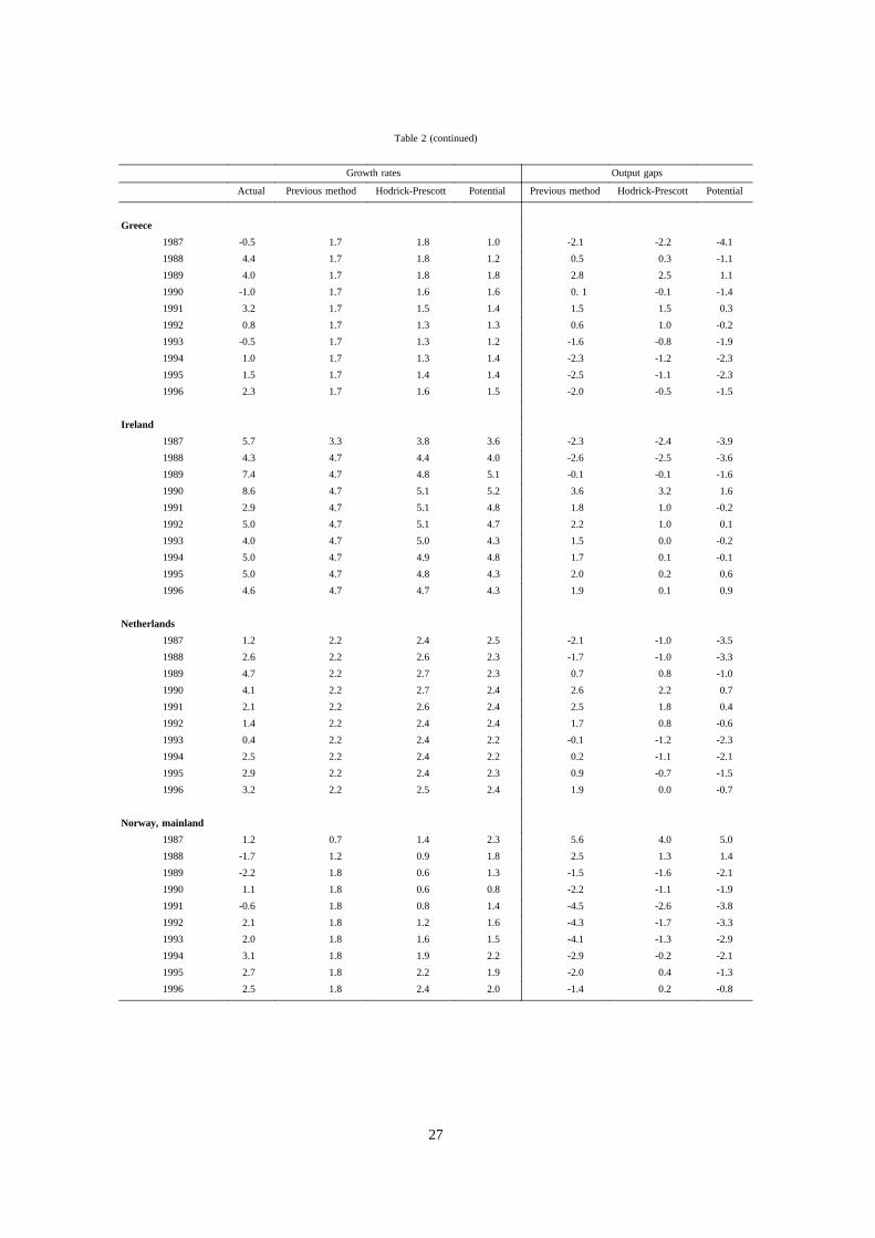
Table 2 (continued)
Growth rates Output gaps
Actual Previous method Hodrick-Prescott Potential Previous method Hodrick-Prescott Potential
Greece
1987 -0.5 1.7 1.8 1.0 -2.1 -2.2 -4.1
1988 4.4 1.7 1.8 1.2 0.5 0.3 -1.1
1989 4.0 1.7 1.8 1.8 2.8 2.5 1.1
1990 -1.0 1.7 1.6 1.6 0. 1 -0.1 -1.4
1991 3.2 1.7 1.5 1.4 1.5 1.5 0.3
1992 0.8 1.7 1.3 1.3 0.6 1.0 -0.2
1993 -0.5 1.7 1.3 1.2 -1.6 -0.8 -1.9
1994 1.0 1.7 1.3 1.4 -2.3 -1.2 -2.3
1995 1.5 1.7 1.4 1.4 -2.5 -1.1 -2.3
1996 2.3 1.7 1.6 1.5 -2.0 -0.5 -1.5
Ireland
1987 5.7 3.3 3.8 3.6 -2.3 -2.4 -3.9
1988 4.3 4.7 4.4 4.0 -2.6 -2.5 -3.6
1989 7.4 4.7 4.8 5.1 -0.1 -0.1 -1.6
1990 8.6 4.7 5.1 5.2 3.6 3.2 1.6
1991 2.9 4.7 5.1 4.8 1.8 1.0 -0.2
1992 5.0 4.7 5.1 4.7 2.2 1.0 0.1
1993 4.0 4.7 5.0 4.3 1.5 0.0 -0.2
1994 5.0 4.7 4.9 4.8 1.7 0.1 -0.1
1995 5.0 4.7 4.8 4.3 2.0 0.2 0.6
1996 4.6 4.7 4.7 4.3 1.9 0.1 0.9
Netherlands
1987 1.2 2.2 2.4 2.5 -2.1 -1.0 -3.5
1988 2.6 2.2 2.6 2.3 -1.7 -1.0 -3.3
1989 4.7 2.2 2.7 2.3 0.7 0.8 -1.0
1990 4.1 2.2 2.7 2.4 2.6 2.2 0.7
1991 2.1 2.2 2.6 2.4 2.5 1.8 0.4
1992 1.4 2.2 2.4 2.4 1.7 0.8 -0.6
1993 0.4 2.2 2.4 2.2 -0.1 -1.2 -2.3
1994 2.5 2.2 2.4 2.2 0.2 -1.1 -2.1
1995 2.9 2.2 2.4 2.3 0.9 -0.7 -1.5
1996 3.2 2.2 2.5 2.4 1.9 0.0 -0.7
Norway, mainland
1987 1.2 0.7 1.4 2.3 5.6 4.0 5.0
1988 -1.7 1.2 0.9 1.8 2.5 1.3 1.4
1989 -2.2 1.8 0.6 1.3 -1.5 -1.6 -2.1
1990 1.1 1.8 0.6 0.8 -2.2 -1.1 -1.9
1991 -0.6 1.8 0.8 1.4 -4.5 -2.6 -3.8
1992 2.1 1.8 1.2 1.6 -4.3 -1.7 -3.3
1993 2.0 1.8 1.6 1.5 -4.1 -1.3 -2.9
1994 3.1 1.8 1.9 2.2 -2.9 -0.2 -2.1
1995 2.7 1.8 2.2 1.9 -2.0 0.4 -1.3
1996 2.5 1.8 2.4 2.0 -1.4 0.2 -0.8
27
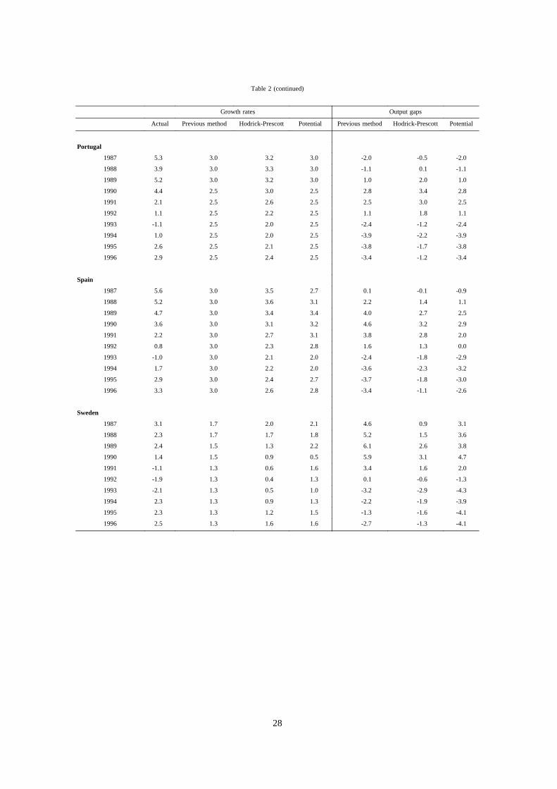
Table 2 (continued)
Growth rates Output gaps
Actual Previous method Hodrick-Prescott Potential Previous method Hodrick-Prescott Potential
Portugal
1987 5.3 3.0 3.2 3.0 -2.0 -0.5 -2.0
1988 3.9 3.0 3.3 3.0 -1.1 0.1 -1.1
1989 5.2 3.0 3.2 3.0 1.0 2.0 1.0
1990 4.4 2.5 3.0 2.5 2.8 3.4 2.8
1991 2.1 2.5 2.6 2.5 2.5 3.0 2.5
1992 1.1 2.5 2.2 2.5 1.1 1.8 1.1
1993 -1.1 2.5 2.0 2.5 -2.4 -1.2 -2.4
1994 1.0 2.5 2.0 2.5 -3.9 -2.2 -3.9
1995 2.6 2.5 2.1 2.5 -3.8 -1.7 -3.8
1996 2.9 2.5 2.4 2.5 -3.4 -1.2 -3.4
Spain
1987 5.6 3.0 3.5 2.7 0.1 -0.1 -0.9
1988 5.2 3.0 3.6 3.1 2.2 1.4 1.1
1989 4.7 3.0 3.4 3.4 4.0 2.7 2.5
1990 3.6 3.0 3.1 3.2 4.6 3.2 2.9
1991 2.2 3.0 2.7 3.1 3.8 2.8 2.0
1992 0.8 3.0 2.3 2.8 1.6 1.3 0.0
1993 -1.0 3.0 2.1 2.0 -2.4 -1.8 -2.9
1994 1.7 3.0 2.2 2.0 -3.6 -2.3 -3.2
1995 2.9 3.0 2.4 2.7 -3.7 -1.8 -3.0
1996 3.3 3.0 2.6 2.8 -3.4 -1.1 -2.6
Sweden
1987 3.1 1.7 2.0 2.1 4.6 0.9 3.1
1988 2.3 1.7 1.7 1.8 5.2 1.5 3.6
1989 2.4 1.5 1.3 2.2 6.1 2.6 3.8
1990 1.4 1.5 0.9 0.5 5.9 3.1 4.7
1991 -1.1 1.3 0.6 1.6 3.4 1.6 2.0
1992 -1.9 1.3 0.4 1.3 0.1 -0.6 -1.3
1993 -2.1 1.3 0.5 1.0 -3.2 -2.9 -4.3
1994 2.3 1.3 0.9 1.3 -2.2 -1.9 -3.9
1995 2.3 1.3 1.2 1.5 -1.3 -1.6 -4.1
1996 2.5 1.3 1.6 1.6 -2.7 -1.3 -4.1
28

Table 3. Regression-based tax elasticitiesa
Corporate tax Household incometax
Social securitycontributions
Indirect taxes
United States 2.3 1.3 1.0 0.4
Japan 1.4 1.1 1.0 0.9
Germany 0.8 1.8 1.2 0.8
France 2.2 1.1 1.3 1.2
Italy 0.7 1.4 0.9 1.1
United Kingdom 0.5 0.9 1.1 1.0
Canada 1.9 0.8 1.2 0.9
Australia -2.3 1.6 n.a. 1.2
Austria 0.4 1.5 1.0 1.2
Belgium 1.9 1.6 1.1 0.7
Denmark 1.9 0.7 0.5 1.0
Finland 1.0 1.1 0.4 0.9
Greece 0.9 1.2 0.8 0.9
Ireland 0.4 1.1 1.3 0.9
Netherlands 0.8 1.3 1.1 0.9
Norwayb 1.2 0.7 1.2 1.1
Portugal 1.5 0.9 0.8 1.0
Spain 0.5 1.8 1.3 0.5
Sweden 0.2 1.2 1.0 1.0
a) Diagnostic statistics available on request. Simple regression of each tax component on output in currentdollars.
b) Mainland GDP.
29
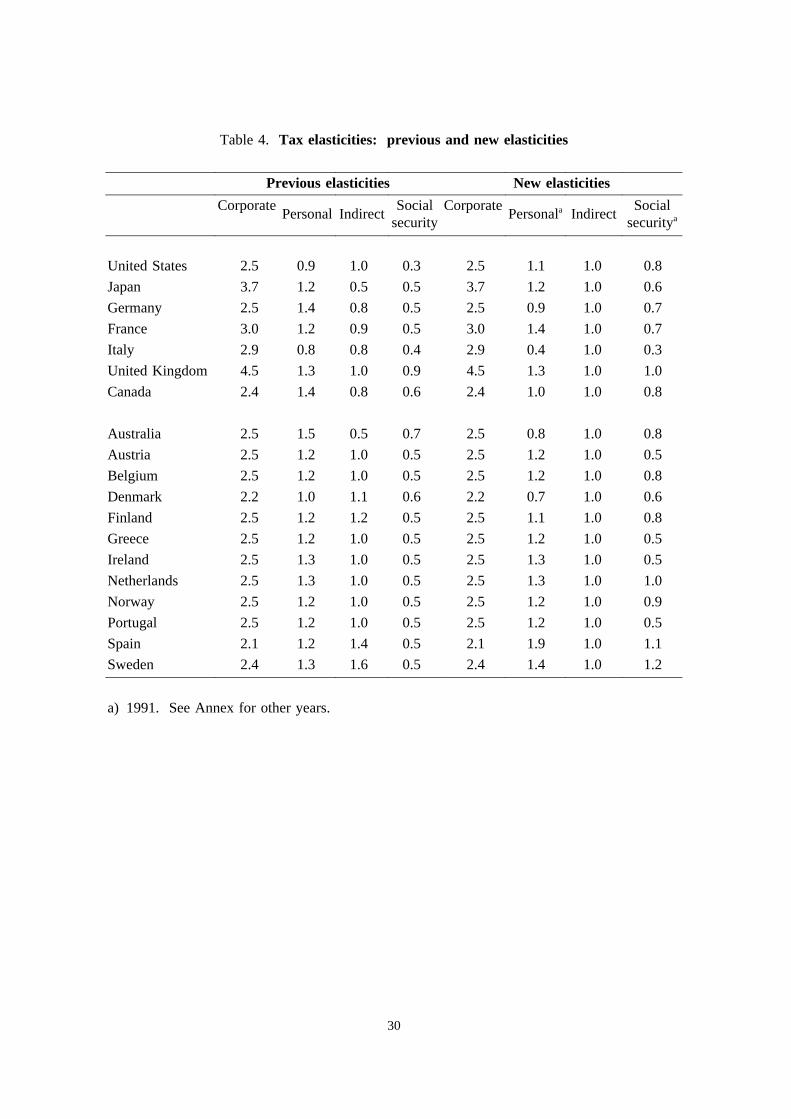
Table 4. Tax elasticities: previous and new elasticities
Previous elasticities New elasticities
CorporatePersonalIndirect
Socialsecurity
CorporatePersonala Indirect
Socialsecuritya
United States 2.5 0.9 1.0 0.3 2.5 1.1 1.0 0.8
Japan 3.7 1.2 0.5 0.5 3.7 1.2 1.0 0.6
Germany 2.5 1.4 0.8 0.5 2.5 0.9 1.0 0.7
France 3.0 1.2 0.9 0.5 3.0 1.4 1.0 0.7
Italy 2.9 0.8 0.8 0.4 2.9 0.4 1.0 0.3
United Kingdom 4.5 1.3 1.0 0.9 4.5 1.3 1.0 1.0
Canada 2.4 1.4 0.8 0.6 2.4 1.0 1.0 0.8
Australia 2.5 1.5 0.5 0.7 2.5 0.8 1.0 0.8
Austria 2.5 1.2 1.0 0.5 2.5 1.2 1.0 0.5
Belgium 2.5 1.2 1.0 0.5 2.5 1.2 1.0 0.8
Denmark 2.2 1.0 1.1 0.6 2.2 0.7 1.0 0.6
Finland 2.5 1.2 1.2 0.5 2.5 1.1 1.0 0.8
Greece 2.5 1.2 1.0 0.5 2.5 1.2 1.0 0.5
Ireland 2.5 1.3 1.0 0.5 2.5 1.3 1.0 0.5
Netherlands 2.5 1.3 1.0 0.5 2.5 1.3 1.0 1.0
Norway 2.5 1.2 1.0 0.5 2.5 1.2 1.0 0.9
Portugal 2.5 1.2 1.0 0.5 2.5 1.2 1.0 0.5
Spain 2.1 1.2 1.4 0.5 2.1 1.9 1.0 1.1
Sweden 2.4 1.3 1.6 0.5 2.4 1.4 1.0 1.2
a) 1991. See Annex for other years.
30
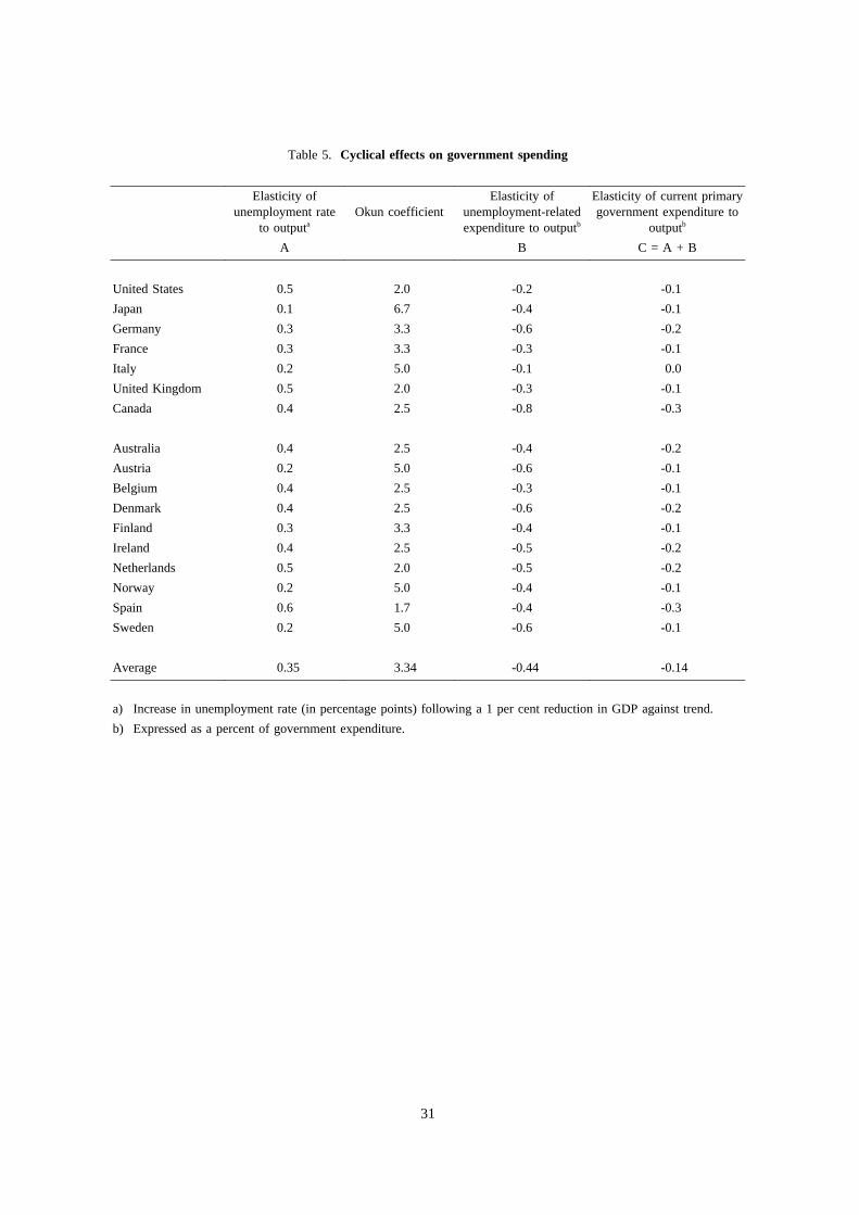
Table 5. Cyclical effects on government spending
Elasticity ofunemployment rate
to outputaOkun coefficient
Elasticity ofunemployment-relatedexpenditure to outputb
Elasticity of current primarygovernment expenditure to
outputb
A B C = A + B
United States 0.5 2.0 -0.2 -0.1
Japan 0.1 6.7 -0.4 -0.1
Germany 0.3 3.3 -0.6 -0.2
France 0.3 3.3 -0.3 -0.1
Italy 0.2 5.0 -0.1 0.0
United Kingdom 0.5 2.0 -0.3 -0.1
Canada 0.4 2.5 -0.8 -0.3
Australia 0.4 2.5 -0.4 -0.2
Austria 0.2 5.0 -0.6 -0.1
Belgium 0.4 2.5 -0.3 -0.1
Denmark 0.4 2.5 -0.6 -0.2
Finland 0.3 3.3 -0.4 -0.1
Ireland 0.4 2.5 -0.5 -0.2
Netherlands 0.5 2.0 -0.5 -0.2
Norway 0.2 5.0 -0.4 -0.1
Spain 0.6 1.7 -0.4 -0.3
Sweden 0.2 5.0 -0.6 -0.1
Average 0.35 3.34 -0.44 -0.14
a) Increase in unemployment rate (in percentage points) following a 1 per cent reduction in GDP against trend.
b) Expressed as a percent of government expenditure.
31
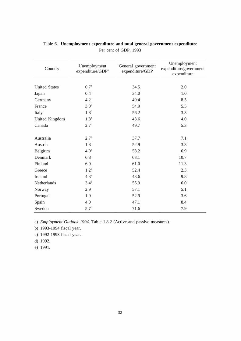
Table 6. Unemployment expenditure and total general government expenditurePer cent of GDP, 1993
CountryUnemployment
expenditure/GDPaGeneral government
expenditure/GDP
Unemploymentexpenditure/government
expenditure
United States 0.7b 34.5 2.0
Japan 0.4c 34.0 1.0
Germany 4.2 49.4 8.5
France 3.0d 54.9 5.5
Italy 1.8d 56.2 3.3
United Kingdom 1.8b 43.6 4.0
Canada 2.7b 49.7 5.3
Australia 2.7c 37.7 7.1
Austria 1.8 52.9 3.3
Belgium 4.0d 58.2 6.9
Denmark 6.8 63.1 10.7
Finland 6.9 61.0 11.3
Greece 1.2d 52.4 2.3
Ireland 4.3e 43.6 9.8
Netherlands 3.4d 55.9 6.0
Norway 2.9 57.1 5.1
Portugal 1.9 52.9 3.6
Spain 4.0 47.1 8.4
Sweden 5.7b 71.6 7.9
a) Employment Outlook 1994. Table 1.8.2 (Active and passive measures).
b) 1993-1994 fiscal year.
c) 1992-1993 fiscal year.
d) 1992.
e) 1991.
32
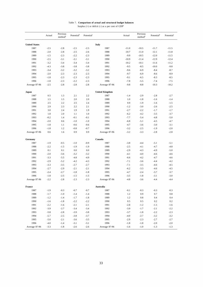
Table 7. Comparison of actual and structural budget balances
Surplus (+) or deficit (-) as a per cent of GDPa
ActualPreviousmethodb
Potentialb Potentialc ActualPreviousmethodb
Potentialb Potentialc
United States Italy
1987 -2.5 -2.8 -2.5 -2.5 1987 -11.0 -10.5 -11.7 -11.5
1988 -2.0 -2.8 -2.5 -2.6 1988 -10.7 -11.0 -12.1 -11.8
1989 -1.5 -2.3 -2.2 -2.3 1989 -9.9 -10.5 -12.0 -11.5
1990 -2.5 -3.1 -3.1 -3.1 1990 -10.9 -11.4 -12.9 -12.4
1991 -3.2 -3.4 -3.4 -3.4 1991 -10.2 -10.1 -11.6 -11.2
1992 -4.3 -3.8 -3.8 -3.8 1992 -9.5 -8.5 -10.0 -9.8
1993 -3.4 -3.2 -3.2 -3.2 1993 -9.6 -6.9 -8.4 -8.7
1994 -2.0 -2.3 -2.3 -2.3 1994 -9.7 -6.9 -8.6 -8.9
1995 -1.8 -2.3 -2.3 -2.3 1995 -9.1 -6.5 -8.3 -8.5
1996 -1.8 -2.3 -2.2 -2.3 1996 -7.8 -5.5 -7.4 -7.5
Average 87-96 -2.5 -2.8 -2.8 -2.8 Average 87-96 -9.8 -8.8 -10.3 -10.2
Japan United Kingdom
1987 0.5 1.3 2.1 2.2 1987 -1.4 -2.9 -2.8 -2.7
1988 1.5 1.5 2.0 2.0 1988 1.0 -1.8 -1.6 -1.4
1989 2.5 2.2 2.5 2.4 1989 0.9 -1.9 -1.6 -1.5
1990 2.9 2.3 2.2 2.1 1990 -1.2 -3.0 -2.6 -2.5
1991 3.0 2.4 1.9 1.9 1991 -2.7 -2.2 -1.7 -1.7
1992 1.8 2.0 1.1 1.0 1992 -6.2 -4.2 -3.5 -3.7
1993 -0.2 1.4 -0.1 -0.1 1993 -7.7 -5.4 -4.8 -5.0
1994 -2.0 0.6 -1.0 -1.0 1994 -6.8 -5.1 -4.5 -4.7
1995 -1.8 1.1 -0.6 -0.6 1995 -4.7 -3.6 -3.0 -3.1
1996 -1.8 1.2 -0.8 -0.7 1996 -3.2 -2.5 -1.9 -2.0
Average 87-96 0.6 1.6 0.9 0.9 Average 87-96 -3.2 -3.3 -2.8 -2.8
Germany Canada
1987 -1.9 -0.5 -1.0 -0.9 1987 -3.8 -4.4 -5.1 -5.1
1988 -2.2 -1.5 -1.9 -1.9 1988 -2.5 -4.1 -4.7 -4.8
1989 0.1 0.1 0.0 0.0 1989 -2.9 -4.3 -4.9 -5.0
1990 -2.0 -3.6 -3.2 -3.2 1990 -4.1 -4.0 -4.6 -4.6
1991 -3.3 -5.5 -4.8 -4.9 1991 -6.6 -4.2 -4.7 -4.6
1992 -2.9 -5.2 -4.2 -4.3 1992 -7.1 -3.6 -4.4 -4.2
1993 -3.3 -3.5 -2.7 -2.7 1993 -7.1 -3.5 -4.6 -4.5
1994 -2.7 -2.9 -2.1 -2.1 1994 -6.2 -3.3 -4.6 -4.5
1995 -2.4 -2.7 -1.8 -1.8 1995 -4.7 -2.4 -3.7 -3.7
1996 -1.8 -2.5 -1.5 -1.5 1996 -3.5 -1.8 -3.1 -3.0
Average 87-96 -2.2 -2.8 -2.3 -2.3 Average 87-96 -4.8 -3.6 -4.4 -4.4
France Australia
1987 -1.9 -0.3 -0.7 -0.7 1987 -0.1 -0.3 -0.3 -0.3
1988 -1.7 -1.0 -1.4 -1.4 1988 1.2 0.9 0.7 0.8
1989 -1.2 -1.4 -1.7 -1.8 1989 1.2 0.8 0.4 0.4
1990 -1.6 -1.8 -2.2 -2.2 1990 0.5 0.5 0.2 0.2
1991 -2.2 -1.6 -2.1 -2.1 1991 -2.8 -1.2 -1.5 -1.6
1992 -3.9 -2.7 -3.4 -3.4 1992 -3.9 -1.7 -2.1 -2.2
1993 -5.8 -2.8 -3.9 -3.8 1993 -3.7 -1.8 -2.2 -2.3
1994 -5.7 -2.5 -3.8 -3.7 1994 -4.0 -2.7 -3.2 -3.2
1995 -5.0 -2.1 -3.6 -3.5 1995 -2.9 -2.3 -2.7 -2.7
1996 -4.0 -1.4 -3.1 -3.1 1996 -1.8 -1.8 -2.0 -2.0
Average 87-96 -3.3 -1.8 -2.6 -2.6 Average 87-96 -1.6 -1.0 -1.3 -1.3
33
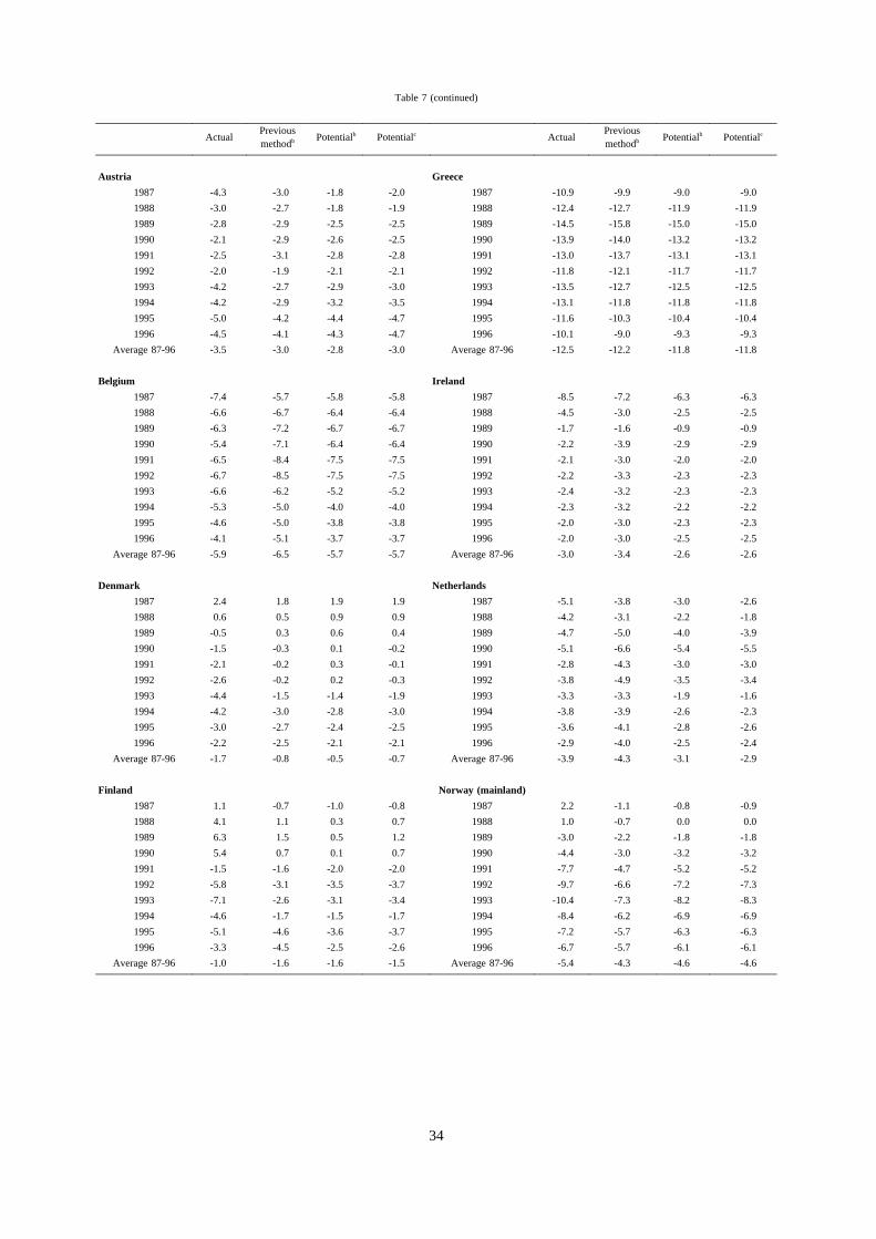
Table 7 (continued)
ActualPreviousmethodb
Potentialb Potentialc ActualPreviousmethodb
Potentialb Potentialc
Austria Greece
1987 -4.3 -3.0 -1.8 -2.0 1987 -10.9 -9.9 -9.0 -9.0
1988 -3.0 -2.7 -1.8 -1.9 1988 -12.4 -12.7 -11.9 -11.9
1989 -2.8 -2.9 -2.5 -2.5 1989 -14.5 -15.8 -15.0 -15.0
1990 -2.1 -2.9 -2.6 -2.5 1990 -13.9 -14.0 -13.2 -13.2
1991 -2.5 -3.1 -2.8 -2.8 1991 -13.0 -13.7 -13.1 -13.1
1992 -2.0 -1.9 -2.1 -2.1 1992 -11.8 -12.1 -11.7 -11.7
1993 -4.2 -2.7 -2.9 -3.0 1993 -13.5 -12.7 -12.5 -12.5
1994 -4.2 -2.9 -3.2 -3.5 1994 -13.1 -11.8 -11.8 -11.8
1995 -5.0 -4.2 -4.4 -4.7 1995 -11.6 -10.3 -10.4 -10.4
1996 -4.5 -4.1 -4.3 -4.7 1996 -10.1 -9.0 -9.3 -9.3
Average 87-96 -3.5 -3.0 -2.8 -3.0 Average 87-96 -12.5 -12.2 -11.8 -11.8
Belgium Ireland
1987 -7.4 -5.7 -5.8 -5.8 1987 -8.5 -7.2 -6.3 -6.3
1988 -6.6 -6.7 -6.4 -6.4 1988 -4.5 -3.0 -2.5 -2.5
1989 -6.3 -7.2 -6.7 -6.7 1989 -1.7 -1.6 -0.9 -0.9
1990 -5.4 -7.1 -6.4 -6.4 1990 -2.2 -3.9 -2.9 -2.9
1991 -6.5 -8.4 -7.5 -7.5 1991 -2.1 -3.0 -2.0 -2.0
1992 -6.7 -8.5 -7.5 -7.5 1992 -2.2 -3.3 -2.3 -2.3
1993 -6.6 -6.2 -5.2 -5.2 1993 -2.4 -3.2 -2.3 -2.3
1994 -5.3 -5.0 -4.0 -4.0 1994 -2.3 -3.2 -2.2 -2.2
1995 -4.6 -5.0 -3.8 -3.8 1995 -2.0 -3.0 -2.3 -2.3
1996 -4.1 -5.1 -3.7 -3.7 1996 -2.0 -3.0 -2.5 -2.5
Average 87-96 -5.9 -6.5 -5.7 -5.7 Average 87-96 -3.0 -3.4 -2.6 -2.6
Denmark Netherlands
1987 2.4 1.8 1.9 1.9 1987 -5.1 -3.8 -3.0 -2.6
1988 0.6 0.5 0.9 0.9 1988 -4.2 -3.1 -2.2 -1.8
1989 -0.5 0.3 0.6 0.4 1989 -4.7 -5.0 -4.0 -3.9
1990 -1.5 -0.3 0.1 -0.2 1990 -5.1 -6.6 -5.4 -5.5
1991 -2.1 -0.2 0.3 -0.1 1991 -2.8 -4.3 -3.0 -3.0
1992 -2.6 -0.2 0.2 -0.3 1992 -3.8 -4.9 -3.5 -3.4
1993 -4.4 -1.5 -1.4 -1.9 1993 -3.3 -3.3 -1.9 -1.6
1994 -4.2 -3.0 -2.8 -3.0 1994 -3.8 -3.9 -2.6 -2.3
1995 -3.0 -2.7 -2.4 -2.5 1995 -3.6 -4.1 -2.8 -2.6
1996 -2.2 -2.5 -2.1 -2.1 1996 -2.9 -4.0 -2.5 -2.4
Average 87-96 -1.7 -0.8 -0.5 -0.7 Average 87-96 -3.9 -4.3 -3.1 -2.9
Finland Norway (mainland)
1987 1.1 -0.7 -1.0 -0.8 1987 2.2 -1.1 -0.8 -0.9
1988 4.1 1.1 0.3 0.7 1988 1.0 -0.7 0.0 0.0
1989 6.3 1.5 0.5 1.2 1989 -3.0 -2.2 -1.8 -1.8
1990 5.4 0.7 0.1 0.7 1990 -4.4 -3.0 -3.2 -3.2
1991 -1.5 -1.6 -2.0 -2.0 1991 -7.7 -4.7 -5.2 -5.2
1992 -5.8 -3.1 -3.5 -3.7 1992 -9.7 -6.6 -7.2 -7.3
1993 -7.1 -2.6 -3.1 -3.4 1993 -10.4 -7.3 -8.2 -8.3
1994 -4.6 -1.7 -1.5 -1.7 1994 -8.4 -6.2 -6.9 -6.9
1995 -5.1 -4.6 -3.6 -3.7 1995 -7.2 -5.7 -6.3 -6.3
1996 -3.3 -4.5 -2.5 -2.6 1996 -6.7 -5.7 -6.1 -6.1
Average 87-96 -1.0 -1.6 -1.6 -1.5 Average 87-96 -5.4 -4.3 -4.6 -4.6
34
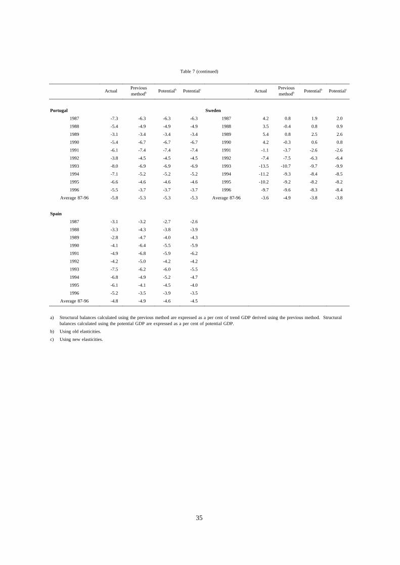
Table 7 (continued)
ActualPreviousmethodb
Potentialb Potentialc ActualPreviousmethodb
Potentialb Potentialc
Portugal Sweden
1987 -7.3 -6.3 -6.3 -6.3 1987 4.2 0.8 1.9 2.0
1988 -5.4 -4.9 -4.9 -4.9 1988 3.5 -0.4 0.8 0.9
1989 -3.1 -3.4 -3.4 -3.4 1989 5.4 0.8 2.5 2.6
1990 -5.4 -6.7 -6.7 -6.7 1990 4.2 -0.3 0.6 0.8
1991 -6.1 -7.4 -7.4 -7.4 1991 -1.1 -3.7 -2.6 -2.6
1992 -3.8 -4.5 -4.5 -4.5 1992 -7.4 -7.5 -6.3 -6.4
1993 -8.0 -6.9 -6.9 -6.9 1993 -13.5 -10.7 -9.7 -9.9
1994 -7.1 -5.2 -5.2 -5.2 1994 -11.2 -9.3 -8.4 -8.5
1995 -6.6 -4.6 -4.6 -4.6 1995 -10.2 -9.2 -8.2 -8.2
1996 -5.5 -3.7 -3.7 -3.7 1996 -9.7 -9.6 -8.3 -8.4
Average 87-96 -5.8 -5.3 -5.3 -5.3 Average 87-96 -3.6 -4.9 -3.8 -3.8
Spain
1987 -3.1 -3.2 -2.7 -2.6
1988 -3.3 -4.3 -3.8 -3.9
1989 -2.8 -4.7 -4.0 -4.3
1990 -4.1 -6.4 -5.5 -5.9
1991 -4.9 -6.8 -5.9 -6.2
1992 -4.2 -5.0 -4.2 -4.2
1993 -7.5 -6.2 -6.0 -5.5
1994 -6.8 -4.9 -5.2 -4.7
1995 -6.1 -4.1 -4.5 -4.0
1996 -5.2 -3.5 -3.9 -3.5
Average 87-96 -4.8 -4.9 -4.6 -4.5
a) Structural balances calculated using the previous method are expressed as a per cent of trend GDP derived using the previous method. Structuralbalances calculated using the potential GDP are expressed as a per cent of potential GDP.
b) Using old elasticities.
c) Using new elasticities.
35
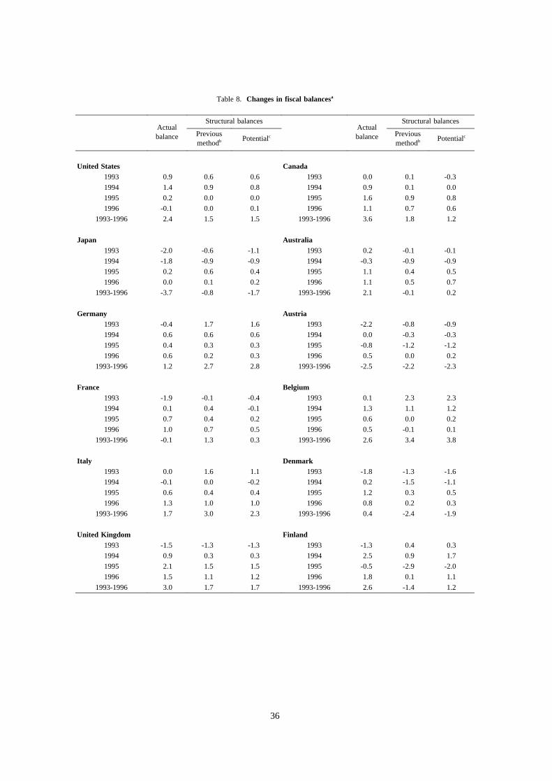
Table 8. Changes in fiscal balancesa
Actualbalance
Structural balancesActualbalance
Structural balances
Previousmethodb
PotentialcPreviousmethodb
Potentialc
United States Canada1993 0.9 0.6 0.6 1993 0.0 0.1 -0.3
1994 1.4 0.9 0.8 1994 0.9 0.1 0.0
1995 0.2 0.0 0.0 1995 1.6 0.9 0.8
1996 -0.1 0.0 0.1 1996 1.1 0.7 0.6
1993-1996 2.4 1.5 1.5 1993-1996 3.6 1.8 1.2
Japan Australia1993 -2.0 -0.6 -1.1 1993 0.2 -0.1 -0.1
1994 -1.8 -0.9 -0.9 1994 -0.3 -0.9 -0.9
1995 0.2 0.6 0.4 1995 1.1 0.4 0.5
1996 0.0 0.1 0.2 1996 1.1 0.5 0.7
1993-1996 -3.7 -0.8 -1.7 1993-1996 2.1 -0.1 0.2
Germany Austria1993 -0.4 1.7 1.6 1993 -2.2 -0.8 -0.9
1994 0.6 0.6 0.6 1994 0.0 -0.3 -0.3
1995 0.4 0.3 0.3 1995 -0.8 -1.2 -1.2
1996 0.6 0.2 0.3 1996 0.5 0.0 0.2
1993-1996 1.2 2.7 2.8 1993-1996 -2.5 -2.2 -2.3
France Belgium1993 -1.9 -0.1 -0.4 1993 0.1 2.3 2.3
1994 0.1 0.4 -0.1 1994 1.3 1.1 1.2
1995 0.7 0.4 0.2 1995 0.6 0.0 0.2
1996 1.0 0.7 0.5 1996 0.5 -0.1 0.1
1993-1996 -0.1 1.3 0.3 1993-1996 2.6 3.4 3.8
Italy Denmark1993 0.0 1.6 1.1 1993 -1.8 -1.3 -1.6
1994 -0.1 0.0 -0.2 1994 0.2 -1.5 -1.1
1995 0.6 0.4 0.4 1995 1.2 0.3 0.5
1996 1.3 1.0 1.0 1996 0.8 0.2 0.3
1993-1996 1.7 3.0 2.3 1993-1996 0.4 -2.4 -1.9
United Kingdom Finland1993 -1.5 -1.3 -1.3 1993 -1.3 0.4 0.3
1994 0.9 0.3 0.3 1994 2.5 0.9 1.7
1995 2.1 1.5 1.5 1995 -0.5 -2.9 -2.0
1996 1.5 1.1 1.2 1996 1.8 0.1 1.1
1993-1996 3.0 1.7 1.7 1993-1996 2.6 -1.4 1.2
36
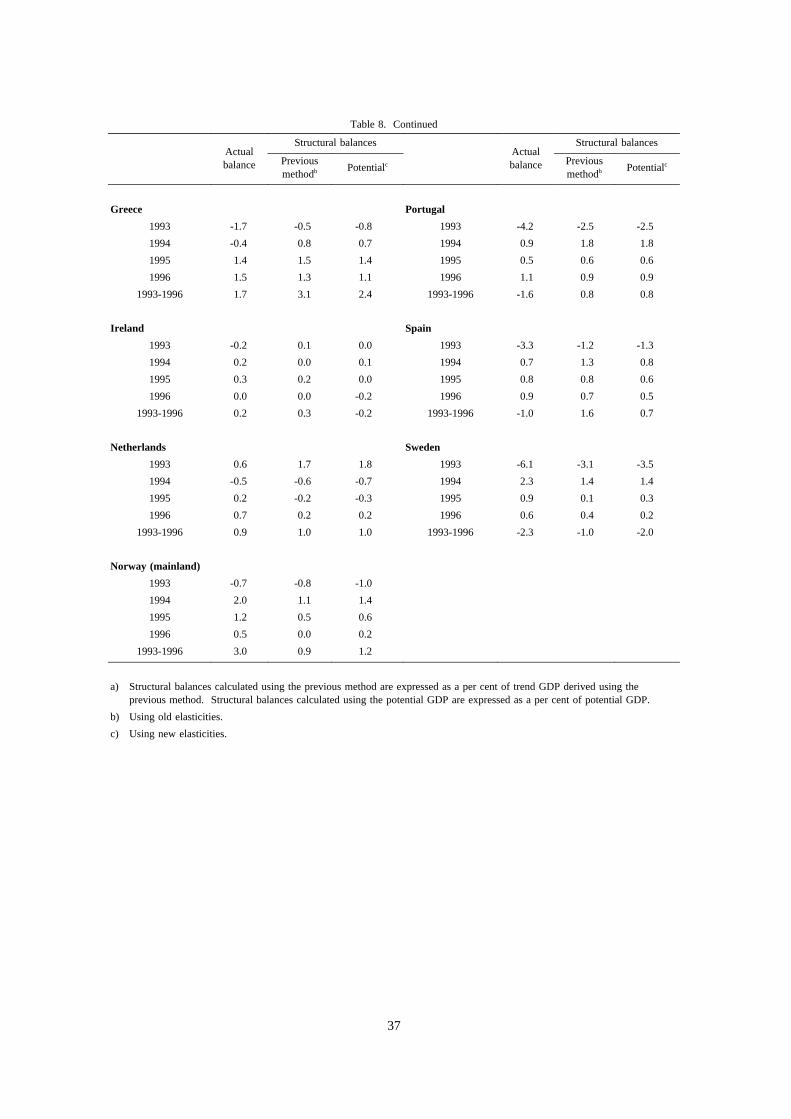
Table 8. Continued
Actualbalance
Structural balancesActualbalance
Structural balances
Previousmethodb
PotentialcPreviousmethodb
Potentialc
Greece Portugal
1993 -1.7 -0.5 -0.8 1993 -4.2 -2.5 -2.5
1994 -0.4 0.8 0.7 1994 0.9 1.8 1.8
1995 1.4 1.5 1.4 1995 0.5 0.6 0.6
1996 1.5 1.3 1.1 1996 1.1 0.9 0.9
1993-1996 1.7 3.1 2.4 1993-1996 -1.6 0.8 0.8
Ireland Spain
1993 -0.2 0.1 0.0 1993 -3.3 -1.2 -1.3
1994 0.2 0.0 0.1 1994 0.7 1.3 0.8
1995 0.3 0.2 0.0 1995 0.8 0.8 0.6
1996 0.0 0.0 -0.2 1996 0.9 0.7 0.5
1993-1996 0.2 0.3 -0.2 1993-1996 -1.0 1.6 0.7
Netherlands Sweden
1993 0.6 1.7 1.8 1993 -6.1 -3.1 -3.5
1994 -0.5 -0.6 -0.7 1994 2.3 1.4 1.4
1995 0.2 -0.2 -0.3 1995 0.9 0.1 0.3
1996 0.7 0.2 0.2 1996 0.6 0.4 0.2
1993-1996 0.9 1.0 1.0 1993-1996 -2.3 -1.0 -2.0
Norway (mainland)
1993 -0.7 -0.8 -1.0
1994 2.0 1.1 1.4
1995 1.2 0.5 0.6
1996 0.5 0.0 0.2
1993-1996 3.0 0.9 1.2
a) Structural balances calculated using the previous method are expressed as a per cent of trend GDP derived using theprevious method. Structural balances calculated using the potential GDP are expressed as a per cent of potential GDP.
b) Using old elasticities.
c) Using new elasticities.
37
38
Tab
le 9
. C
yclic
al c
ompo
nent
of b
udge
t bal
ance
s (a
)
Sur
plus
(+
) or
def
icit
(-)
as a
per
cent
age
of p
oten
tial G
DP
Est
imat
es a
nd p
roje
ctio
ns
1979
1980
1981
1982
1983
1984
1985
1986
1987
1988
1989
1990
1991
1992
1993
1994
1995
1996
Uni
ted
Sta
tes
(c)
0.9
-0.2
-0.5
-2.0
-1.5
-0.4
-0.2
-0.2
0.0
0.6
0.8
0.6
0.2
-0.5
-0.2
0.3
0.6
0.4
Japa
n (c
)0
.0-0
.2-0
.3-0
.6-1
.2-1
.1-0
.9-1
.7-1
.8-0
.60
.10
.81
.20
.9-0
.1-1
.0-1
.2-1
.1G
erm
any
(c)
1.8
1.0
-0.2
-1.7
-1.7
-1.2
-1.0
-0.7
-0.9
-0.3
0.1
1.1
1.5
1.3
-0.6
-0.6
-0.6
-0.2
Fra
nce
0.9
0.4
-0.4
0.3
-0.4
-1.0
-1.2
-1.1
-1.2
-0.3
0.5
0.6
-0.1
-0.5
-1.8
-1.8
-1.4
-0.9
Italy
0.4
0.8
0.5
0.0
-0.3
-0.3
-0.2
0.0
0.4
0.7
1.1
1.0
0.7
0.2
-0.7
-0.6
-0.4
-0.2
Uni
ted
Kin
gdom
1.1
-0.5
-2.2
-2.6
-1.8
-1.6
-0.9
0.1
1.3
2.5
2.4
1.3
-0.9
-2.2
-2.3
-1.9
-1.5
-1.2
Ca
na
da
1.1
0.2
0.2
-2.6
-2.5
-1.0
0.1
0.5
1.2
2.2
2.0
0.5
-1.8
-2.5
-2.3
-1.5
-0.9
-0.4
Tot
al o
f abo
ve c
ount
ries
0.8
0.1
-0.5
-1.4
-1.4
-0.8
-0.5
-0.5
-0.3
0.4
0.8
0.8
0.4
-0.2
-0.6
-0.5
-0.3
-0.2
Aus
tral
ia0
.30
.20
.2-0
.8-1
.7-0
.50
.2-0
.20
.20
.50
.80
.4-1
.1-1
.6-1
.3-0
.7-0
.20
.2A
ustr
ia0
.90
.9-0
.6-1
.3-1
.4-1
.9-1
.7-2
.0-2
.1-1
.1-0
.30
.40
.30
.1-1
.1-0
.8-0
.5-0
.1B
elgi
um (
b)
0.5
2.0
0.7
0.4
-1.7
-0.4
-0.9
-1.3
-1.5
-0.2
0.4
0.9
0.9
0.8
-1.2
-1.1
-0.7
-0.4
De
nm
ark
1
.60
.4-1
.2-0
.9-0
.70
.21
.11
.60
.5-0
.3-0
.9-1
.3-1
.9-2
.2-2
.3-1
.2-0
.5-0
.1
Fin
land
0.5
1.2
0.3
0.3
0.1
0.2
0.5
0.8
1.9
3.8
6.0
5.3
0.5
-1.9
-3.3
-2.6
-1.2
-0.7
Gre
ece
0
.80
.4-0
.3-0
.9-1
.3-1
.1-0
.7-0
.9-1
.5-0
.40
.4-0
.50
.1-0
.1-0
.7-0
.9-0
.9-0
.7Ir
elan
d 0
.90
.70
.70
.2-1
.4-0
.8-0
.7-2
.9-1
.9-1
.8-0
.70
.8-0
.10
.1-0
.10
.00
.30
.4N
ethe
rland
s1
.71
.0-0
.6-2
.5-2
.6-1
.9-1
.7-1
.5-2
.3-2
.2-0
.70
.40
.2-0
.4-1
.5-1
.4-1
.0-0
.5
No
rwa
y (e
)-0
.20
.10
.1-0
.4-0
.20
.62
.93
.73
.21
.0-1
.1-1
.2-2
.3-2
.1-1
.8-1
.4-0
.9-0
.6P
ortu
gal
0.9
1.7
1.4
1.1
0.0
-1.8
-2.1
-1.7
-0.9
-0.5
0.3
1.1
1.2
0.6
-0.9
-1.7
-1.8
-1.6
Sp
ain
-1
.2-1
.6-2
.4-2
.5-2
.5-2
.6-2
.3-1
.9-0
.50
.61
.51
.71
.20
.0-1
.8-2
.0-1
.9-1
.6S
we
de
n1
.00
.6-0
.4-0
.8-0
.80
.91
.11
.52
.32
.73
.03
.61
.4-0
.9-3
.0-2
.3-1
.8-1
.1
Tot
al o
f abo
ve s
mal
ler
coun
trie
s0
.30
.2-0
.7-1
.2-1
.6-1
.2-0
.9-0
.8-0
.40
.10
.81
.10
.3-0
.5-1
.6-1
.4-1
.1-0
.7T
otal
of a
bove
Eur
opea
n co
untr
ies
0.9
0.4
-0.6
-1.1
-1.3
-1.1
-0.9
-0.6
-0.3
0.4
0.9
1.1
0.5
-0.2
-1.4
-1.3
-1.0
-0.7
To
tal o
f a
bo
ve O
EC
D c
ou
ntr
ies
0.8
0.1
-0.5
-1.4
-1.4
-0.8
-0.6
-0.5
-0.3
0.4
0.8
0.8
0.4
-0.2
-0.8
-0.6
-0.4
-0.3
a) O
EC
D S
ecre
taria
t est
imat
es o
f the
cyc
lical
com
pone
nt o
f gen
eral
gov
ernm
ent f
inan
cial
bal
ance
s. T
he e
stim
ates
are
sur
roun
ded
by la
rge
mar
gins
of e
rror
, ref
lect
ing
unce
rtai
nty
as to
the
pres
ent s
ize
and
futu
re
grow
th o
f pot
entia
l out
put,
and
the
degr
ee to
whi
ch e
limin
atio
n of
the
outp
ut g
ap w
ould
tran
slat
e in
to e
nhan
ced
tax
reve
nues
and
red
uced
exp
endi
ture
. b)
Exc
lude
s de
posi
t ins
uran
ce o
utla
ys.
Rec
eipt
s re
latin
g to
Ope
ratio
n D
eser
t Sto
rm, a
mou
ntin
g to
0.6
per
cen
t of G
DP
in 1
991,
are
exc
lude
d.c)
Exc
lude
s ex
pend
iture
rel
ated
to O
pera
tion
Des
ert S
torm
in 1
991
amou
ntin
g to
0.2
per
cen
t of G
DP
for
Japa
n an
d to
0.4
per
cen
t of G
DP
for
Ger
man
y.d)
Incl
udes
pro
ceed
s of
priv
atis
atio
ns a
nd s
ales
of o
ther
ass
ets
(BF
32.
2 bi
llion
in 1
993,
BF
57
billi
on in
199
4 an
d B
F13
.5 in
199
5).
e) A
s a
perc
enta
ge o
f mai
nlan
d G
DP
. T
he fi
nanc
ial b
alan
ces
show
n ex
clud
e re
venu
es fr
om o
il pr
oduc
tion.
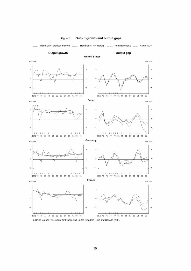
France
a. Using lambda=25, except for France and United Kingdom (100) and Canada (200).
1971 73 75 77 79 81 83 85 87 89 91 93 95
−5
0
5
Per cent
−5
0
5
1971 73 75 77 79 81 83 85 87 89 91 93 95
−5
0
5
−5
0
5
Per cent
Germany
1971 73 75 77 79 81 83 85 87 89 91 93 95
−5
0
5
Per cent
−5
0
5
1971 73 75 77 79 81 83 85 87 89 91 93 95
−5
0
5
−5
0
5
Per cent
Japan
1971 73 75 77 79 81 83 85 87 89 91 93 95
−5
0
5
Per cent
−5
0
5
1971 73 75 77 79 81 83 85 87 89 91 93 95
−5
0
5
−5
0
5
Per cent
Output growth and output gaps
Output growthUnited States
Trend GDP: previous method Trend GDP: HP filter(a) Potential output Actual GDP
1971 73 75 77 79 81 83 85 87 89 91 93 95
−5
0
5
Per cent
−5
0
5
Figure 1.
Output gap
1971 73 75 77 79 81 83 85 87 89 91 93 95
−5
0
5
−5
0
5
Per cent
39
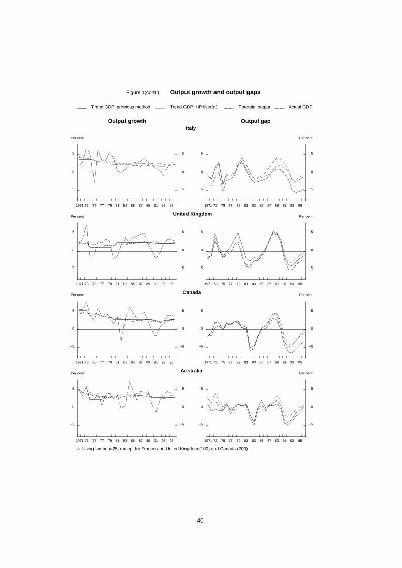
Australia
a. Using lambda=25, except for France and United Kingdom (100) and Canada (200).
1971 73 75 77 79 81 83 85 87 89 91 93 95
−5
0
5
Per cent
−5
0
5
1971 73 75 77 79 81 83 85 87 89 91 93 95
−5
0
5
−5
0
5
Per cent
Canada
1971 73 75 77 79 81 83 85 87 89 91 93 95
−5
0
5
Per cent
−5
0
5
1971 73 75 77 79 81 83 85 87 89 91 93 95
−5
0
5
−5
0
5
Per cent
United Kingdom
1971 73 75 77 79 81 83 85 87 89 91 93 95
−5
0
5
Per cent
−5
0
5
1971 73 75 77 79 81 83 85 87 89 91 93 95
−5
0
5
−5
0
5
Per cent
Output growth and output gaps
Output growthItaly
Trend GDP: previous method Trend GDP: HP filter(a) Potential output Actual GDP
1971 73 75 77 79 81 83 85 87 89 91 93 95
−5
0
5
Per cent
−5
0
5
Figure 1(cont.).
Output gap
1971 73 75 77 79 81 83 85 87 89 91 93 95
−5
0
5
−5
0
5
Per cent
40
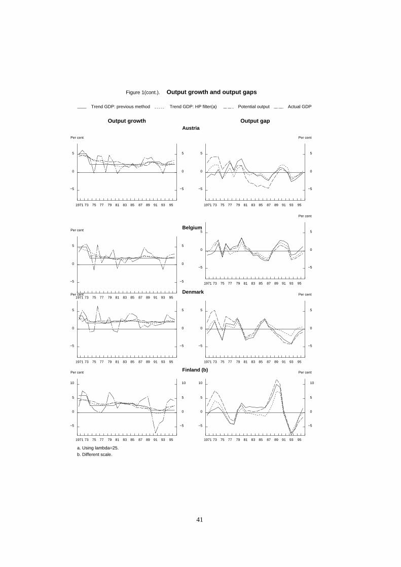
Finland (b)
a. Using lambda=25.b. Different scale.
1971 73 75 77 79 81 83 85 87 89 91 93 95
−5
0
5
10
Per cent
−5
0
5
10
1971 73 75 77 79 81 83 85 87 89 91 93 95
−5
0
5
10
−5
0
5
10
Per cent
Denmark
1971 73 75 77 79 81 83 85 87 89 91 93 95
−5
0
5
Per cent
−5
0
5
1971 73 75 77 79 81 83 85 87 89 91 93 95
−5
0
5
−5
0
5
Per cent
Belgium
1971 73 75 77 79 81 83 85 87 89 91 93 95
−5
0
5
Per cent
−5
0
5
1971 73 75 77 79 81 83 85 87 89 91 93 95
−5
0
5
−5
0
5
Per cent
Output growth and output gaps
Output growthAustria
Trend GDP: previous method Trend GDP: HP filter(a) Potential output Actual GDP
1971 73 75 77 79 81 83 85 87 89 91 93 95
−5
0
5
Per cent
−5
0
5
Figure 1(cont.).
Output gap
1971 73 75 77 79 81 83 85 87 89 91 93 95
−5
0
5
−5
0
5
Per cent
41
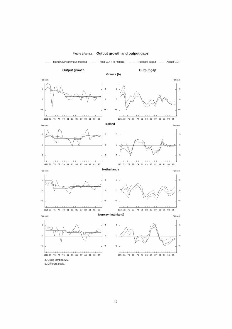
Norway (mainland)
a. Using lambda=25.b. Different scale.
1971 73 75 77 79 81 83 85 87 89 91 93 95
−5
0
5
Per cent
−5
0
5
1971 73 75 77 79 81 83 85 87 89 91 93 95
−5
0
5
−5
0
5
Per cent
Netherlands
1971 73 75 77 79 81 83 85 87 89 91 93 95
−5
0
5
Per cent
−5
0
5
1971 73 75 77 79 81 83 85 87 89 91 93 95
−5
0
5
−5
0
5
Per cent
Ireland
1971 73 75 77 79 81 83 85 87 89 91 93 95
−5
0
5
Per cent
−5
0
5
1971 73 75 77 79 81 83 85 87 89 91 93 95
−5
0
5
−5
0
5
Per cent
Output growth and output gaps
Output growthGreece (b)
Trend GDP: previous method Trend GDP: HP filter(a) Potential output Actual GDP
1971 73 75 77 79 81 83 85 87 89 91 93 95
−5
0
5
Per cent
−5
0
5
Figure 1(cont.).
Output gap
1971 73 75 77 79 81 83 85 87 89 91 93 95
−5
0
5
−5
0
5
Per cent
42

Sweden
a. Using lambda=25.b. Different scale.
1971 73 75 77 79 81 83 85 87 89 91 93 95
−5
0
5
Per cent
−5
0
5
1971 73 75 77 79 81 83 85 87 89 91 93 95
−5
0
5
−5
0
5
Per cent
Spain
Trend GDP: previous method Trend GDP: HP filter(a) Potential output Actual GDP
1971 73 75 77 79 81 83 85 87 89 91 93 95
−5
0
5
Per cent
−5
0
5
1971 73 75 77 79 81 83 85 87 89 91 93 95
−5
0
5
−5
0
5
Per cent
Output growth and output gaps
Output growthPortugal (b)
1971 73 75 77 79 81 83 85 87 89 91 93 95
−5
0
5
10
Per cent
−5
0
5
10
Figure 1(cont.).
Output gap
1971 73 75 77 79 81 83 85 87 89 91 93 95
−5
0
5
10
−5
0
5
10
Per cent
43
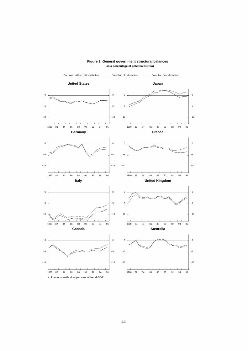
as a percentage of potential GDP(a)
Figure 2. General government structural balances
United States
Previous method, old elasticities Potential, old elasticities. Potential, new elasticities
1980 82 84 86 88 90 92 94 96
−10
−5
0
−10
−5
0
Japan
1980 82 84 86 88 90 92 94 96
−10
−5
0
−10
−5
0
Germany
1980 82 84 86 88 90 92 94 96
−10
−5
0
−10
−5
0
France
1980 82 84 86 88 90 92 94 96
−10
−5
0
−10
−5
0
Italy
1980 82 84 86 88 90 92 94 96
−10
−5
0
−10
−5
0
United Kingdom
1980 82 84 86 88 90 92 94 96
−10
−5
0
−10
−5
0
Canada
a. Previous method as per cent of trend GDP.
1980 82 84 86 88 90 92 94 96
−10
−5
0
−10
−5
0
Australia
1980 82 84 86 88 90 92 94 96
−10
−5
0
−10
−5
0
44
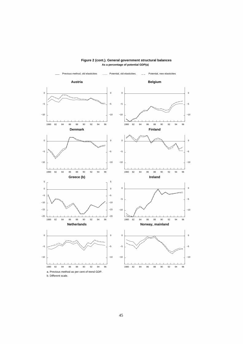
As a percentage of potential GDP(a)
Figure 2 (cont.). General government structural balances
Austria
Previous method, old elasticities Potential, old elasticities. Potential, new elasticities
1980 82 84 86 88 90 92 94 96
−10
−5
0
−10
−5
0
Belgium
1980 82 84 86 88 90 92 94 96
−10
−5
0
−10
−5
0
Denmark
1980 82 84 86 88 90 92 94 96
−10
−5
0
−10
−5
0
Finland
1980 82 84 86 88 90 92 94 96
−10
−5
0
−10
−5
0
Greece (b)
1980 82 84 86 88 90 92 94 96
−20
−15
−10
−5
0
5
−20
−15
−10
−5
0
5
Ireland
1980 82 84 86 88 90 92 94 96
−10
−5
0
−10
−5
0
Netherlands
a. Previous method as per cent of trend GDP.b. Different scale.
1980 82 84 86 88 90 92 94 96
−10
−5
0
−10
−5
0
Norway, mainland
1980 82 84 86 88 90 92 94 96
−10
−5
0
−10
−5
0
45

As a percentage of potential GDP(a)
Figure 2 (cont.). General government structural balances
Portugal (b)
Previous method, old elasticities Potential, old elasticities. Potential, new elasticities
1980 82 84 86 88 90 92 94 96
−20
−15
−10
−5
0
5
−20
−15
−10
−5
0
5
Spain
a. Previous method as per cent of trend GDP.b. Different scale.
1980 82 84 86 88 90 92 94 96
−10
−5
0
−10
−5
0
Sweden
1980 82 84 86 88 90 92 94 96
−10
−5
0
−10
−5
0
46
Annex 1
Determination of Income-tax and Social Security Contributions Elasticities
1. This annex sets out the method that has been used to estimate the output elasticities forhousehold-income tax and social security contributions referred to in Table 5 of the main text. The methodinvolves a number of steps, which will be discussed subsequently below. The first step consists ofcalculating the marginal and average tax rates (contribution rates) of a representative household at variouspoints on the distribution of gross earnings. The second step is to weight these marginal and average taxrates (contribution rates) together with the weights derived from an estimated income-distribution function.The third and final step is to derive the output (GDP) elasticities of income taxes and social securitycontributions, allowing for cross-country variation in the responsiveness of employment and wages tofluctuations in real output.
2. The results are rather crude and to be considered as indicative, as a number of simplifyingassumptions had to be made. First of all, the representative household is taken to be one consisting of afull-time male worker, a working spouse with gross earnings equalling half of those of her husband, andtwo children. Second, the calculations refer to "production workers" only, and hence ignore the taxsituation of, amongst others, the self-employed. Finally, the income-distribution functions are fitted on alimited number of observations (the first, fifth and ninth deciles), and are held constant over time.
The tax situation of individual households
3. The average and marginal tax rates at different levels of gross earnings depend on the specificfeatures of the tax system, including tax credits, rebates, tax progression, tax ceilings and tax allowancesfor a dependent spouse and children, etc. The tax position of individual households on various points ofthe income distribution have been estimated on the basis of data compiled by DAFFE, modelling the taxsystems in 15 individual countries, i.e. the major seven, Australia, Belgium, Denmark, Finland, Netherlands,Norway, Spain and Sweden [see DAFFE/CFA/WP2/WD(93)20]. Simulations have been carried out for16 points on the distribution of gross earnings, with respect to both income tax and social securitycontributions, for the years 1978, 1981, 1985, 1989 and 1991, and where data were available also for 1992.Income tax comprises both local and central government taxes and social security contributions includethose made by both employees and employers.
The "weighted average" tax situation
4. In order to calculate the marginal and average rates for an "average" household, the distributionof gross earnings across households has to be established. This distribution, however, is not known formost countries. For each country a log-normal income distribution function could be fitted, on the basisof the two parameters that were known: the ratio of the income level at the first decile to the medianincome level and the ratio of the ninth decile to the median level (taken from theEmployment OutlookofJuly 1993, Table 5.2).
47

5. The weights required to calculate average and marginal tax rates, however, cannot be deriveddirectly from the log-normal distribution function. What is needed is the frequency distribution of currencyunits earned-- denoted as the "first-moment" distribution. It can be shown that the original distributionand the first-moment distribution have exactly the same standard deviation (σ), while the mean of thefirst-moment distribution exceeds that of the original distribution (u) by the variation coefficient (σ2).
6. The weighted average earnings elasticities, finally, are calculated as follows (Table A1):
in which:ε = the earnings elasticity of income taxes or social security contributions;ϒi = the weight of earnings-level i in total earnings according to the first-moment distribution;ti = income-tax payments (social security contributions) per household at earnings level i;yi = earnings per household at earnings level i;dti/dyi = the marginal tax rate (contribution rate) at point i on the earnings distribution;ti/yi = the average tax rate (contribution rate) at point i on the earnings distribution.
From earnings- to output-elasticities
7. Output growth will only to a limited extent be reflected in enhanced earnings and governmentrevenues, as there are a number of "leakages" to be taken into account. First, output growth typically leadsto a less than proportional increase in employment due to the presence of hoarded labour within firms.Second, a given rate of growth of employment typically produces a less than proportional increase inwages per household in as much as the number of households earning an income from employment alsoincreases. Third, and related to the second point, an increase in the number of wage earners,a priori, leadsto a proportional rather than a progressive increase in payments to the government. If it is assumed thatthe newly employed are subject to the same distribution of earnings as the already employed, theappropriate elasticity of tax and social security contributionsvis-à-vis employment is unity, and thefollowing relationship will hold:
α = EE(EW.ε + 1) = EE.EW.ε + EE
where: α = the output-elasticity of income taxes or social security contributions;ε = the earnings elasticity of income taxes or social security contributions;EE = the output-elasticity of employment;EW = the employment-elasticity of wages.
This formula expresses that the impact of a 1 per cent increase in output on tax proceeds is a compositeof two factors: i) an increase in earnings per worker and the associated progressive increase in governmentproceeds; and ii) an increase in the number of workers in each earnings bracket and the associatedproportional increase in government proceeds.
48
8. The calculations based on this relationship for 1991 are presented in Table A2 and the results forall years in Table A3. The output-elasticities of employment and the employment-elasticities of wages havebeen taken from Elmeskov and Pichelmann (1993), with two exceptions. First, for Japan theemployment-elasticity of wages has been set at 2, on the basis of simulations with the new version of theINTERLINK supply block, which accounts for the high responsiveness of overtime (and hence wages perhousehold) to variations in activity [see Turneret al.(1993) for a description of these simulations]. Second,for Australia the employment elasticity of wages has been put at zero, which is probably more realistic thanthe negative value which is found on the basis of simple regression.
49
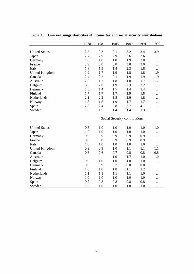
Table A1. Gross-earnings elasticities of income tax and social security contributions
1978 1981 1985 1989 1991 1992
United States 2.5 2.3 2.1 3.2 3.4 3.9Japan 2.7 2.9 2.9 2.6 2.6 ..Germany 1.8 1.8 1.8 1.9 2.0 ..France 2.9 3.0 3.0 3.0 3.0 ..Italy 1.8 1.9 1.4 2.3 1.8 ..United Kingdom 1.9 1.7 1.9 1.8 1.8 1.9Canada 2.4 2.2 2.1 1.9 1.9 1.9Australia 2.0 1.7 1.8 1.8 1.7 1.7Belgium 3.6 2.0 1.9 2.3 2.2 ..Denmark 1.5 1.4 1.5 1.4 1.4 ..Finland 1.7 1.7 1.7 1.9 1.8 ..Netherlands 2.1 2.2 1.8 1.9 1.8 ..Norway 1.8 1.8 1.9 1.7 1.7 ..Spain 2.8 2.4 2.8 3.7 4.1 ..Sweden 1.6 1.5 1.4 1.4 1.3 ..
Social Security contributions
United States 0.8 1.0 1.0 1.0 1.0 1.0Japan 1.0 1.0 1.0 1.0 1.0 ..Germany 0.9 0.9 0.9 0.9 0.9 ..France 0.8 0.8 0.9 0.9 0.9 ..Italy 1.0 1.0 1.0 1.0 1.0 ..United Kingdom 0.9 0.9 1.0 1.1 1.1 1.1Canada 0.6 0.6 0.7 0.8 0.8 0.8Australia .. .. 1.0 1.7 1.0 1.0Belgium 0.9 1.0 1.0 1.0 1.0 ..Denmark 0.9 0.9 0.7 0.0 0.0 ..Finland 1.0 1.0 1.0 1.1 1.2 ..Netherlands 1.1 1.1 1.1 1.1 1.0 ..Norway 1.0 1.0 1.0 1.0 1.0 ..Spain 0.7 0.8 0.8 0.8 0.8 ..Sweden 1.0 1.0 1.0 1.0 1.0 ..
50
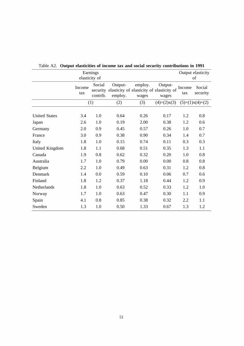
Table A2. Output elasticities of income tax and social security contributions in 1991
Earningselasticity of
Output elasticityof
Incometax
Socialsecuritycontrib.
Output-elasticity of
employ.
employ.elasticity of
wages
Output-elasticity of
wages
Incometax
Socialsecurity
(1) (2) (3) (4)=(2)x(3) (5)=(1)x(4)+(2)
United States 3.4 1.0 0.64 0.26 0.17 1.2 0.8
Japan 2.6 1.0 0.19 2.00 0.38 1.2 0.6
Germany 2.0 0.9 0.45 0.57 0.26 1.0 0.7
France 3.0 0.9 0.38 0.90 0.34 1.4 0.7
Italy 1.8 1.0 0.15 0.74 0.11 0.3 0.3
United Kingdom 1.8 1.1 0.68 0.51 0.35 1.3 1.1
Canada 1.9 0.8 0.62 0.32 0.20 1.0 0.8
Australia 1.7 1.0 0.79 0.00 0.00 0.8 0.8
Belgium 2.2 1.0 0.49 0.63 0.31 1.2 0.8
Denmark 1.4 0.0 0.59 0.10 0.06 0.7 0.6
Finland 1.8 1.2 0.37 1.18 0.44 1.2 0.9
Netherlands 1.8 1.0 0.63 0.52 0.33 1.2 1.0
Norway 1.7 1.0 0.63 0.47 0.30 1.1 0.9
Spain 4.1 0.8 0.85 0.38 0.32 2.2 1.1
Sweden 1.3 1.0 0.50 1.33 0.67 1.3 1.2
51
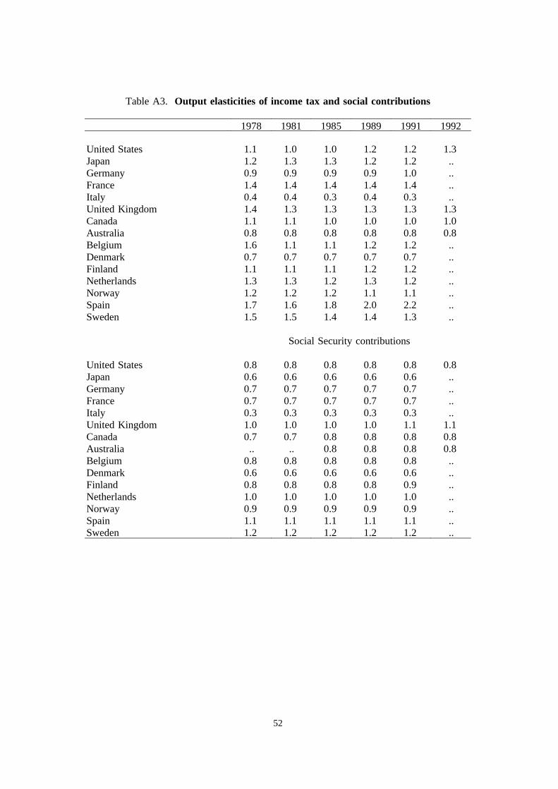
Table A3. Output elasticities of income tax and social contributions
1978 1981 1985 1989 1991 1992
United States 1.1 1.0 1.0 1.2 1.2 1.3Japan 1.2 1.3 1.3 1.2 1.2 ..Germany 0.9 0.9 0.9 0.9 1.0 ..France 1.4 1.4 1.4 1.4 1.4 ..Italy 0.4 0.4 0.3 0.4 0.3 ..United Kingdom 1.4 1.3 1.3 1.3 1.3 1.3Canada 1.1 1.1 1.0 1.0 1.0 1.0Australia 0.8 0.8 0.8 0.8 0.8 0.8Belgium 1.6 1.1 1.1 1.2 1.2 ..Denmark 0.7 0.7 0.7 0.7 0.7 ..Finland 1.1 1.1 1.1 1.2 1.2 ..Netherlands 1.3 1.3 1.2 1.3 1.2 ..Norway 1.2 1.2 1.2 1.1 1.1 ..Spain 1.7 1.6 1.8 2.0 2.2 ..Sweden 1.5 1.5 1.4 1.4 1.3 ..
Social Security contributions
United States 0.8 0.8 0.8 0.8 0.8 0.8Japan 0.6 0.6 0.6 0.6 0.6 ..Germany 0.7 0.7 0.7 0.7 0.7 ..France 0.7 0.7 0.7 0.7 0.7 ..Italy 0.3 0.3 0.3 0.3 0.3 ..United Kingdom 1.0 1.0 1.0 1.0 1.1 1.1Canada 0.7 0.7 0.8 0.8 0.8 0.8Australia .. .. 0.8 0.8 0.8 0.8Belgium 0.8 0.8 0.8 0.8 0.8 ..Denmark 0.6 0.6 0.6 0.6 0.6 ..Finland 0.8 0.8 0.8 0.8 0.9 ..Netherlands 1.0 1.0 1.0 1.0 1.0 ..Norway 0.9 0.9 0.9 0.9 0.9 ..Spain 1.1 1.1 1.1 1.1 1.1 ..Sweden 1.2 1.2 1.2 1.2 1.2 ..
52
References
BLANCHARD, O., "Suggestions for a new set of fiscal indicators",OECD Department of Economics andStatistics Working PaperNo. 79, 1990.
CANOVA, F., "Detrending and business cycle facts",CEPR Discussion PaperNo. 782, 1993.
CHOURAQUI, J.C., R. HAGEMANN and N. SARTOR, "Indicators of fiscal policy: a reexamination",OECD Department of Economics and Statistics Working PaperNo. 78, 1990.
ELMESKOV, J. and M. MACFARLAN, "Unemployment persistence",OECD Economic Studies,No. 21(Winter 1993).
ELMESKOV, J., "High and persistent unemployment: assessment of the problem and its causes",OECDEconomics Department Working PaperNo. 132, 1993.
HODRICK, R. and E. PRESCOTT, "Post-war US business cycles: an empirical investigation", WorkingPaper, Carnegie Mellon University, 1980.
KYDLAND F. and C. PRESCOTT, "Business cycles: real facts and a monetary myth", FederalReserve Bank of Minneapolis,Quarterly Review(Spring), pp 3-18, 1990.
NELSON, C. and C.I. PLOSSER, "Trends and random walks in macroeconomic series",Journal ofMonetary Economics 10, pp 139-162, 1982.
OECD, Working Party No. 2 on Tax Analysis and Tax Statistics of the Committee of Fiscal Affairs, TaxEquation Spreadsheets, Paris, 1993 [DAFFE/CFA/WP2/WD(93)20].
OECD,Employment Outlook,Paris, July 1993.
PRICE, W.R. and P. MULLER, "Structural budget indicators and the interpretation of fiscal policy stancein OECD economies",OECD Economic Studies,No. 3, Autumn 1994.
TORRES, R and J.P. MARTIN, "Potential output in the seven major OECD countries",OECD EconomicStudiesNo. 14, Spring 1990, pp 127-149.
TORRES, R., P. JARRETT and W. SUYKER, "Modelling business sector supply for the smaller OECDcountries",Department of Economics and Statistics Working PaperNo. 71, 1989.
TURNER, D., P. RICHARDSON and S. RAUFFET, "The role of real and nominal rigidities inmacroeconomic adjustment", OECDEconomic Studies,No. 21, Winter 1993.
TURNER, D., P. RICHARDSON and S. RAUFFET, "Modelling the supply side of the seven major OECDeconomies", OECD Economics Department Working Paper (forthcoming).
53